JPL Publication 14-18

Geostationary Coastal and Air Pollution Events (GEO-CAPE) Sensitivity Analysis Experiment

Meemong Lee and Kevin Bowman

National Aeronautics and Space Administration Jet Propulsion Laboratory California Institute of Technology Pasadena, California

October 2014

https://ntrs.nasa.gov/search.jsp?R=20160001773 2018-07-30T12:45:22+00:00Z

ii

The research described in this publication was carried out at the Jet Propulsion Laboratory, California Institute of Technology, under a contract with the National Aeronautics and Space Administration. Reference herein to any specific commercial product, process, or service by trade name, trademark, manufacturer, or otherwise does not constitute or imply its endorsement by the United States Government or the Jet Propulsion Laboratory, California Institute of Technology. © 2014 California Institute of Technology. Government sponsorship acknowledged

iii

Table of Contents

1 Introduction ....................................................................................................................... 1

2 Adjoint Sensitivity Analysis Framework .......................................................................... 2

2.1 Emission Inventory ......................................................................................................................... 2 2.2 Cost Function and Gradient Cost Function .................................................................................... 3 2.3 Software Process ............................................................................................................................ 5 2.4 Adjoint-Sensitivity Configuration ..................................................................................................... 6

3 Model Parameters .............................................................................................................. 8

4 Sensitivity Analysis Experiments ....................................................................................11

4.1 Sensitivity Analysis of Observation Scenarios ............................................................................. 12 4.2 Sensitivity Analysis of Instrument Options ................................................................................... 20

5 Appendices .......................................................................................................................22

Appendix A. Checkpoint files ................................................................................................................... 22 Appendix B. NOx Emission Inventory ..................................................................................................... 23 Appendix C. Tracer name list .................................................................................................................. 24 Appendix D. Acronyms and Abbreviations .............................................................................................. 26

Figures

Figure 1. Adjoint Sensitivity Analysis Framework ......................................................................................... 2 Figure 2. Adjoint Sensitivity Analysis Processes .......................................................................................... 6 Figure 3. External Configuration of the Sensitivity Function ......................................................................... 7 Figure 4. NOX emission sources over N. America in 2006/08 ..................................................................... 9 Figure 5. Total Anthropogenic NOx Emission and Diurnal Scale Factor of Five Fuel Combustion

Sources ................................................................................................................................................ 10 Figure 6. Weekly Mean Ozone Sensitivity to the Global NOx Emissions during One Month

(2006/May) ........................................................................................................................................... 11 Figure 7. CASTNet Sites (red squares) and EPA Region 9 (California, Arizona, & Nevada shown in

pinkish highlight) .................................................................................................................................. 12 Figure 8. Analysis Regions Marked in Dotted Circle on the Global NOx Emission Background ................ 12 Figure 9. Five Regions of the NOx Emission and Daily Contribution Ratios during 2006/05

to USA O3 ............................................................................................................................................. 13 Figure 10. Sensitivity Comparison between Observations at the EPA-9 Region and at

CASTNet Sites ..................................................................................................................................... 14 Figure 11. Column O3 over the EPA-09 Region (Top) and Contributions from NOx Emissions

(Bottom) ............................................................................................................................................... 15 Figure 12. Column O3 over the EPA-09 Region (Top) and Contributions from NOx Emissions

(Bottom) ............................................................................................................................................... 16 Figure 13. The Column O3 change in EPA-09 region due to NOx emissions from EPA09 and

China for 2006/05 (Top) and 2006/05/20 (Bottom) .............................................................................. 17 Figure 14. Sensitivity Comparison between the Surface O3 (Top) and Column O3

Observations (Bottom) ......................................................................................................................... 18 Figure 15. Sensitivity to the State-Wide NOx Emission: Surface O3 (top) and Column O3 (Bottom) ......... 19 Figure 16. Diagonal Vector of the Averaging Kernel of Three Instruments ................................................ 20 Figure 17. Sensitivity Comparison of the Three Instruments Relative to an Ideal Instrument .................... 21

iv

Tables Table 1. Sensitivity Analysis Study Cases .................................................................................................... 1 Table 2. Emission Inventories ....................................................................................................................... 3 Table 3. 57 Emissions Mapped to the Tracers and the Emission Types ...................................................... 8

1

1 Introduction GEO-CAPE is a NASA decadal survey mission to be designed to provide surface reflectance at high spectral, spatial, and temporal resolutions from a geostationary orbit necessary for studying regional-scale air quality issues and their impact on global atmospheric composition processes. GEO-CAPE's Atmospheric Science Questions explore the influence of both gases and particles on air quality, atmospheric composition, and climate [http://geo-cape.larc.nasa.gov/atmosphere].

1. What are the temporal and spatial variations of emissions of gases and aerosols that are important for air quality and climate?

2. How do physical, chemical, and dynamical processes determine tropospheric composition and air quality over scales ranging from urban to continental, diurnally to seasonally?

3. How does air pollution drive climate forcing, and how does climate change affect air quality on a continental scale?

4. How can observations from space improve air quality forecasts and assessments for societal benefit?

5. How does intercontinental transport affect surface air quality?

6. How do episodic events (such as wild fires, dust outbreaks, and volcanic eruptions) affect atmospheric composition and air quality?

The GEO-CAPE Observing System Simulation Experiment (OSSE) team at JPL has developed a comprehensive sensitivity analysis framework to quantitatively evaluate the impact of the GEO-CAPE observations. Employing the sensitivity framework, a wide range of OSSEs have been performed varying the target location, analysis region and duration, and evaluation criteria as illustrated in Table 1 with four study cases. This report describes the mathematical and computational processes of the sensitivity analysis framework and discusses the findings with respect to the OSSE configuration and the sensitivity of the observed ozone to NOx surface emissions.

Table 1. Sensitivity Analysis Study Cases

Case Target location

Analysis region

Analysis duration

Evaluation Resolution

1 N. America N. America 2006/08/01-06 57 Emission types 0.5 ° × 0.667° 2 Washington

D.C. N. America 2006/07/21-26 TIR, UV, VIS 0.5 ° × 0.667°

3 USA Global 2006/05/01-31 GEO-CAPE, CASTNet 2° × 2.5° 4 EPA-09 region Global 2006/05/01-31 Surface O3, Column O3 2° × 2.5°

2

2 Adjoint Sensitivity Analysis Framework The Adjoint Sensitivity Analysis framework was developed based on the GEOS-Chem-Adjoint version 34 system (GCA), which provides the adjoint models for dynamics, emission, and chemistry. Figure 1 describes the relationship between the forecast loop and the adjoint loop during the sensitivity analysis process. The forecast loop simulates the state of the atmospheric composition forward in time and saves the checkpoint files (Appendix A) required for the adjoint loop at each simulation time. The adjoint loop computes a sensitivity function of the target observation (described in an observation scenario) and propagates the sensitivity backward in time employing the adjoint models.

Figure 1. Adjoint Sensitivity Analysis Framework

2.1 Emission Inventory The Emission Inventory is organized for anthropogenic and biogenic groups as summarized in Table 2. The anthropogenic group includes emissions from the human activities on land, air, and ocean. The biogenic group includes emission sources and sinks from plant, soil, lightning, and fire. There are five global inventories and five regional inventories for the anthropogenic emissions. Also additional inventories are available for emissions from aircraft, shipping, and bio-fuel. Each emission is scaled by a set of temporal scale factors (e.g., annual, seasonal, weekday, weekend, and hourly) and/or a set of spatial scale factors (e.g., soil type and leaf area index). The emissions within each model are organized in multiple sectors with sector-specific temporal scale factors and applicability regions (Appendix B).

At each simulation time step, the GCA forecasts the state of 43 tracers (33 chemical components and 10 aerosol compounds as shown in Appendix C) with the dynamics model, emission model, and chemical processing model. The dynamics model performs the advection process and the convection process based on the GEOS-5 meteorology fields generated by the Goddard Earth Observing System (GEOS) version 5.

3

Table 2. Emission Inventories

Type Model Scale Misc. description

Anthro-global

EMEP annual Europe EDGAR v4.2 hourly NEI2005 seasonal USA RETRO IPCC future

Anthro-regional

STREETS monthly SE Asia CAC Canada Bravo Mexico Cooke GC/OC N. America

Aircraft Ship ICOADS Biofuel

Plant MEGAN AEF_ISOP,

AEF_MONOT Leaf_area_index

Biomass burn GFED2 Monthly GFED3 (optional) 3 hourly

Lightning Scale, loc_redist, CTH param

NOx

Soil Olson Fertilizer NOx Acronyms used in this table are explained in Appendix D.

2.2 Cost Function and Gradient Cost Function The mathematical definition of the cost function and gradient cost function within the adjoint sensitivity framework is described below following the work of Henze et al.1

The adjoint model is used to calculate gradients of the error weighted squared difference between model predictions and observations with respect to emissions. An adjoint model is an efficient means of calculating the sensitivities of this type of model response with respect to numerous model parameters simultaneously, affording optimization of parameters on a resolution commensurate with that of the forward model itself. This allows refinement of both the overall magnitude and the spatial distributions of emissions, distinguishing between different emission source sectors, and quantification of the influence of other uncertain model parameters such as initial conditions and heterogeneous uptake coefficients.

A chemical transport model can be viewed as a numerical operator, F, acting on a vector of initial concentrations, c0, and a vector of parameters, p, to yield an estimate of the evolved concentrations at a later time, N,

1 D. K. Henze, J. H. Seinfeld, and D. T. Shindell, “Inverse modeling and mapping US air quality influences of inorganic PM2.5 precursor emissions using the adjoint of GEOS-Chem,” Atmos. Chem. Phys., vol. 9, pp. 5877–5903, 2009.

4

, p) (1) where c is the vector of all K tracer concentrations, c = [c1 , . . ., ck , . . ., cK] and cn is the concentration at time step n. In practice, F comprises many individual operators representing various physical processes. For the moment, let Fn represent a portion of the discrete forward model that advances the concentration vector from time step n to step n + 1.

(2) The adjoint model is used to calculate the sensitivity of a scalar model response function, J, with respect to the model parameters, p. The response function may depend only upon a subset of concentrations, , and may include a term explicitly depending upon the parameters.

(3)

Assuming the parameters are constants, J_p (p) does not have a time step index. In practice the definitions of are very application-specific. For the following derivation it is simply assumed that the response domain includes all species at all times and the parameters are constant, such that

(4)

The purpose of the adjoint model is to calculate the sensitivity of the response with respect to the model parameters. As will become evident, it is first necessary to calculate the sensitivity of the model response with respect to species concentrations at every time step n in the model,

(5)

note:

= 0 when n’ < n

The Jacobian matrix of the model operator around any given time step can be written as and similarly,

/ = )/ (6)

/ = )/ (7)

Using the chain rule, the sum on the right hand side of Eq. (5) is expanded,

(8)

The sensitivity of the response with respect to the model parameters (assumed here not to depend on the time step n) can then be written as

5

(9)

In this context, the adjoint method is essentially just an approach to evaluating Eqs. (8) and (9), that is computationally efficient when dim{c} and dim{p} > dim {J }. The adjoint sensitivity variables are defined as λc

n = ∆cnJ and λp= ∆pJ, where the subscripts c and p indicate sensitivity with respect to c and p, respectively. Initializing

(9)

adjoint sensitivities are found by evaluating the following update formulas iteratively from n = N, . . ., 1

(10)

(11)

The

terms are referred to as the adjoint forcings as their role in the adjoint model is

analogous to that of emissions in the forward model. While calculation of adjoint values using this algorithm is straightforward, there are a few subtleties worth mentioning. First, evaluating sensitivities with respect to model parameters requires having first calculated sensitivities with respect to concentrations. Since evaluation of Eq. (8) is much more computationally expensive than evaluation of Eq. (9), the overall computational cost is largely invariant to the number of parameters considered. Second, while solving Eq. (11) iteratively along with Eq. (10) is not necessary, it is computationally preferable as values of

and need not be stored for more

than a single step.

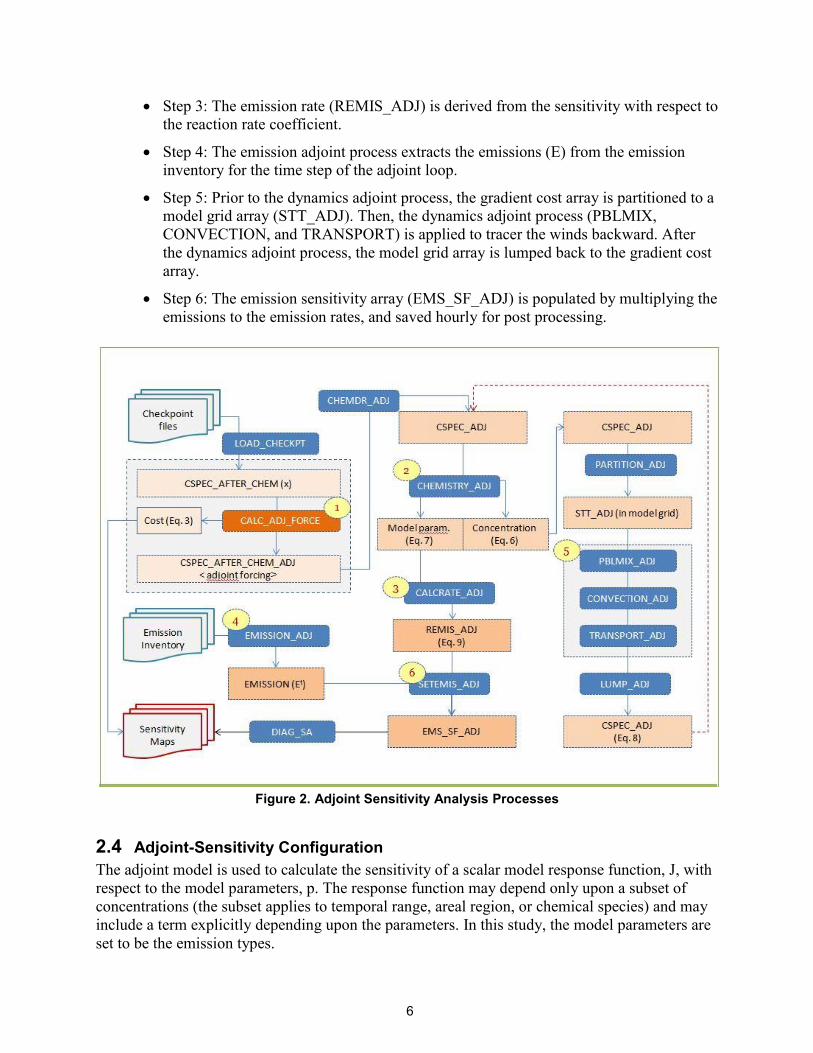
2.3 Software Process The sensitivity analysis framework has extended the GCA software system to support external configuration of the cost function and to track intermediate stage of the gradient cost array and emission status. The extension required a careful mapping between the adjoint sensitivity function described above and the data variables inside of the GCA software implementation. Figure 2 describes the process flow of the adjoint loop within the GCA framework, which includes the six steps described below:

Step 1: The sensitivity function (CALC_ADJ_FORCE) computes the cost and adjoint force, and updates the total cost and the gradient cost array (CSPEC_ADJ).

Step 2: The chemistry adjoint process derives two types of sensitivities from the adjoint force, a sensitivity with respect to concentration and a sensitivity with respect to the reaction rate coefficient.

6

Step 3: The emission rate (REMIS_ADJ) is derived from the sensitivity with respect to the reaction rate coefficient.

Step 4: The emission adjoint process extracts the emissions (E) from the emission inventory for the time step of the adjoint loop.

Step 5: Prior to the dynamics adjoint process, the gradient cost array is partitioned to a model grid array (STT_ADJ). Then, the dynamics adjoint process (PBLMIX, CONVECTION, and TRANSPORT) is applied to tracer the winds backward. After the dynamics adjoint process, the model grid array is lumped back to the gradient cost array.

Step 6: The emission sensitivity array (EMS_SF_ADJ) is populated by multiplying the emissions to the emission rates, and saved hourly for post processing.

Figure 2. Adjoint Sensitivity Analysis Processes

2.4 Adjoint-Sensitivity Configuration The adjoint model is used to calculate the sensitivity of a scalar model response function, J, with respect to the model parameters, p. The response function may depend only upon a subset of concentrations (the subset applies to temporal range, areal region, or chemical species) and may include a term explicitly depending upon the parameters. In this study, the model parameters are set to be the emission types.

7

The sensitivity function has been implemented to accept four types of control parameters, a time range, a sample list, a pressure range, and an averaging kernel to explore the impact of sampling scenarios and instrument options. As shown in Figure3, a target location is represented with a sample list which specifies the sample locations in latitude and longitude and a time range during which the observations should be made. The time range can also be applied during the evaluation of the instrument options.

Cost type 1: The cost of the tracer O3 is defined to be the mean concentration in the unit of parts per billion (ppb) where the O3 concentration is retrieved from the CSPEC array (values are stored in molecules/cm3).

Cost type 2: The cost of the tracer O3 is defined to be the sum of the concentration within the target area in the unit of ppb where the O3 concentration is retrieved from the STT array (values are stored in v/v).

Figure 3. External Configuration of the Sensitivity Function

8

3 Model Parameters In general, the parameters of a chemical transport model include emissions, boundary conditions, initial conditions, and rate parameters for deposition and chemical reactions. For this study, the parameters initially considered are scaling factors for the emissions of SOx, NOx, and NH3 from the source sectors listed in Table 2. The emissions extracted from the emission inventories are internally organized into a two-dimensional emission array (E), the relevant tracers for the first dimension and the emission type for the second dimension.

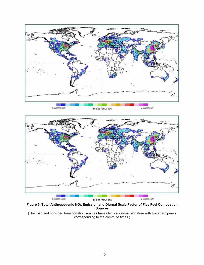
Currently there are 57 emissions and Table 3 shows their mapping to the two dimensional array composed of the tracers and the emission types. Figure 4 shows the spatial distribution and magnitude range (in moles/cm2/s) of the six emission types in North America. Figure 5 shows the spatial distribution of the global anthropogenic NOx and associated diurnal signatures of five major anthropogenic sources, road and non-road transportations, industry, power generation, and residential.

Table 3. 57 Emissions Mapped to the Tracers and the Emission Types

Tracer* anthro biofuel Aircraft/ship Plant Biomass burn

lightning soil

NOx 25 26 24 27 23 22 CO 38 29 30 ALK4 34 35 36 ISOP 31 32 33 ACET 37 38 39 MEK 40 41 42 ALD2 43 44 45 PRPE 46 47 48 C3H8 49 50 51 C2H6 55 56 57 SO2 5,6 7 9 8 NH3 1 4 2 3 BCPI 10 14 18 OCPI 12 16 20 BCPO 11 15 19 OCPO 13 17 21 Note: Appendix C lists the full names of the tracers listed in the first column.

9

Figure 4. NOX emission sources over N. America in 2006/08

(The value range of the color bar is between 0 and the value shown in parenthesis next to each emission type.)

10

Figure 5. Total Anthropogenic NOx Emission and Diurnal Scale Factor of Five Fuel Combustion

Sources

(The road and non-road transportation sources have identical diurnal signature with two sharp peaks corresponding to the commute times.)

11

4 Sensitivity Analysis Experiments The NOx emission sensitivity analysis tracks the adjoint sensitivity stored in the EMS_SF_ADJ variable hourly, integrating the sensitivities for the three types of NOx emission sources, anthropogenic, bio-fuel, and biomass-burn. The NOx emissions from aircraft, lightning, and soil are not included for the analysis. Figure 6 illustrates the weekly mean sensitivities of the continental United States ozone (CONUS--O3) during one month (2006/05) to the global NOx emissions. As the assimilation process progresses backward in time starting on May/31, 2006, the impact of the global NOx emissions starts to appear. The impact of the NOx emissions in China starts in the second week, and it exceeds the impact of the NOx emissions in the EPA-9 region.

Figure 6. Weekly Mean Ozone Sensitivity to the Global NOx Emissions

during One Month (2006/May)

The impact of an observation scenario can be evaluated by performing the above sensitivity analysis and analyzing the temporal and spatial relationships of the resulting sensitivity results. Section 4.1 discusses the OSSEs performed for seven observation scenarios to quantify the impact of their sampling strategies. Section 4.2 discusses the OSSES performed for three instrument systems to quantify the impact of their averaging kernels.

12

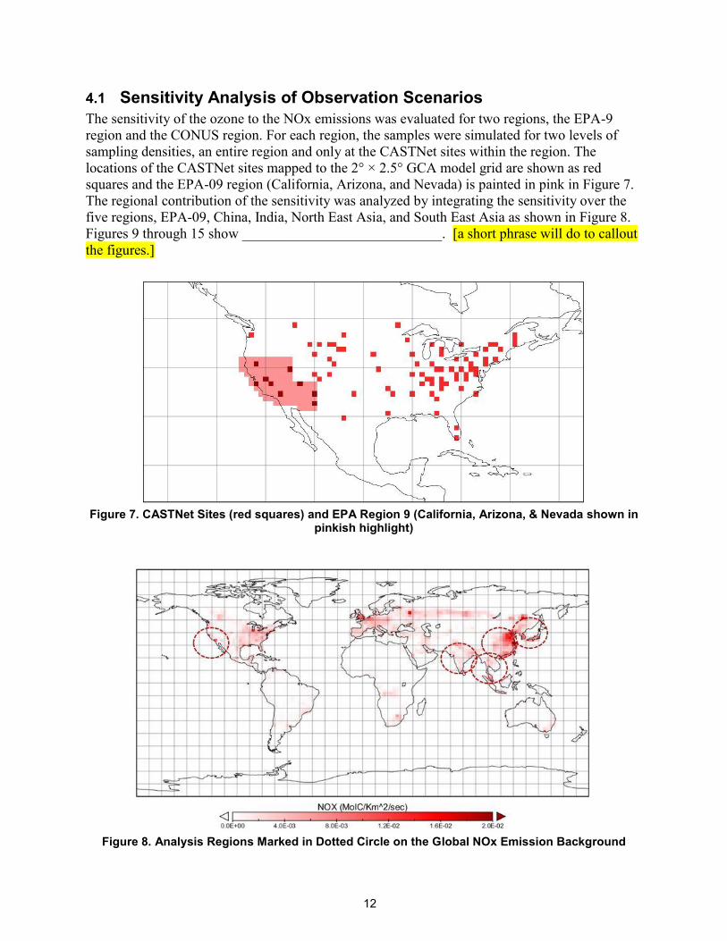
4.1 Sensitivity Analysis of Observation Scenarios The sensitivity of the ozone to the NOx emissions was evaluated for two regions, the EPA-9 region and the CONUS region. For each region, the samples were simulated for two levels of sampling densities, an entire region and only at the CASTNet sites within the region. The locations of the CASTNet sites mapped to the 2° × 2.5° GCA model grid are shown as red squares and the EPA-09 region (California, Arizona, and Nevada) is painted in pink in Figure 7. The regional contribution of the sensitivity was analyzed by integrating the sensitivity over the five regions, EPA-09, China, India, North East Asia, and South East Asia as shown in Figure 8. Figures 9 through 15 show ____________________________. [a short phrase will do to callout the figures.]

Figure 7. CASTNet Sites (red squares) and EPA Region 9 (California, Arizona, & Nevada shown in

pinkish highlight)

Figure 8. Analysis Regions Marked in Dotted Circle on the Global NOx Emission Background

13

Observations Column O3 (hourly during May of 2006) Target area USA (93 CASTNet sites) Analysis duration 2006/05/01-30 Analysis regions EPA-9, China, India, North East Asia, South East Asia Findings:

1. The sensitivity to the EPA-9-NOx stays about constant over the entire month.

2. It takes ~8 days for the Chinese NOx emission starts to impact the USA O3 and it has higher impact than the EPA-9 NOx emission.

3. The sensitivity to the Chinese NOx emission dominates the sensitivities to other regions in Asia.

Figure 9. Five Regions of the NOx Emission and Daily Contribution Ratios

during 2006/05 to USA O3

14

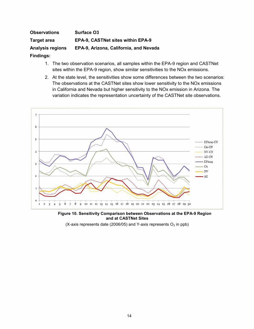
Observations Surface O3 Target area EPA-9, CASTNet sites within EPA-9 Analysis regions EPA-9, Arizona, California, and Nevada Findings:

1. The two observation scenarios, all samples within the EPA-9 region and CASTNet sites within the EPA-9 region, show similar sensitivities to the NOx emissions.

2. At the state level, the sensitivities show some differences between the two scenarios: The observations at the CASTNet sites show lower sensitivity to the NOx emissions in California and Nevada but higher sensitivity to the NOx emission in Arizona. The variation indicates the representation uncertainty of the CASTNet site observations.

Figure 10. Sensitivity Comparison between Observations at the EPA-9 Region

and at CASTNet Sites

(X-axis represents date (2006/05) and Y-axis represents O3 in ppb)

15

Observations Column O3 (hourly, during May 2006) Target area EPA-9 Analysis duration 2006/05/01-30 Analysis regions Globe, China, EPA-9 Findings:

1. The average column ozone over the EPA-9 region is between 45 ppb and 60 ppb.

2. ~5 ppb is sensitive to the global NOx emission.

3. ~1 ppb is sensitive to the EPA-9 NOx emission.

4. ~1 ppb is sensitive to the Chinese NOx emission.

Figure 11. Column O3 over the EPA-09 Region (Top) and Contributions

from NOx Emissions (Bottom)

(The X-axis represents the day of the month (2006/05), and the Y-axis represents the O3 in ppb.)

16

Observations Column O3 (hourly, during May 2006) Target area EPA-9 Analysis duration 2006/05/01-30 Analysis regions China, EPA-09, Arizona, California, Nevada Findings:

1. It takes ~7 days for the Chinese NOx emission to impact the column ozone in the EPA-9 region.

2. After 20 days, the impact of the Chinese NOx emission is higher than that of EPA-9 region.

3. The majority of the EPA-9 NOX emission impact is due to the California NOX emission.

Figure 12. Column O3 over the EPA-09 Region (Top) and Contributions

from NOx Emissions (Bottom)

(The X-axis represents the day of the month (2006/05) and the Y-axis represents the O3 in ppb.)

17

Observations Column O3 (hourly, during May 2006) Target area EPA-9 Analysis duration 2006/05/01-30 Analysis regions China, EPA-09 Findings:

1. There is a strong diurnal signature where the peak influence from the EPA09 NOx occurs at 9AM PST and the peak influence from the Chinese NOx occurs at 10 PM PST.

2. The diurnal signature reflects the diurnal cycle pattern of the NOx emission in Figure 5.

Figure 13. The Column O3 change in EPA-09 region due to NOx emissions from EPA09 and China

for 2006/05 (Top) and 2006/05/20 (Bottom)

18

Observations Surface O3 and Column O3 (hourly, during May 2006) Target area EPA-9 Analysis duration 2006/05/01-30 Analysis regions Global, China, EPA-09 Findings:

1. The impact of global NOx and EPA09 NOx to EPA09 O3 at surface shows ~2 ppb higher than over the column.

2. The impact the Chinese NOx to EPA09 03 at surface is negligible, but it is > 1 ppb over the column and the impact starts to appear about one week after the start of the adjoint loop.

Figure 14. Sensitivity Comparison between the Surface O3 (Top) and

Column O3 Observations (Bottom)

(The dJ represents the daily average O3 change due to the NOx emissions.)

19

Observation Surface O3 and Column O3 (hourly, during May 2006) Target area EPA-9 Analysis duration 2006/05/01-30 Analysis regions Arizona, California, & Nevada Findings:

1. The California NOx emission impacts > 50% of the surface ozone but < 40% of the column ozone.

2. The Arizona NOx emission shows much greater impact to the column ozone between May/14-19.

Figure 15. Sensitivity to the State-Wide NOx Emission: Surface O3 (top) and Column O3 (Bottom)

20

4.2 Sensitivity Analysis of Instrument Options An instrument option is represented with a pressure range and an averaging kernel to formulate an observation operator (H). For example, an instrument whose averaging kernel is a function of the log of the O3 profile in the unit of “v/v”, the observation operator can be simulated by convolving the averaging kernel to the log of the model forecast that has been mapped to the pressure levels of the averaging kernel. The gradient cost is modified by the gradient of the observation operator function that has been mapped back to the model pressure profile.

The sensitivity of the averaging kernel of an observing system was analyzed for three types of instruments, thermal infra-red (TIR), ultra-violet (UV), and visible (VIS) spectrometers. Figure 16 shows the diagonal vector of the averaging kernel of the three instrument types where the X-axis represents 120 pressure-level bins (1000 hPa to 0.0 hPa), and the Y-axis represents the normalized amplitude. Figure 17 compares the sensitivity of the observed ozone from the above three instruments to the ideal instrument where the observed ozone of each instrument is simulated by convolving the ideal observation with the respective averaging kernel.

Figure 16. Diagonal Vector of the Averaging Kernel of Three Instruments

(X-axis represents the pressure levels and the Y-axis represents the amplitude)

21

Observations Column O3 at 3:00 PM on 2007/07/26 Target area Washington D.C. Analysis duration 2007/07/21- 26 Analysis instruments IDEAL, TIR, UV, VIS Findings:

1. The ideal case indicates that the column O3 in Washington, D.C. is affected by the NOx emissions in N. America throughout the 6 day period, and the strongest emission sources were three days away.

2. The TIR is >90% responsive to the distant emission sources and <70% responsive to the near ones.

3. The UV is as responsive as TIR over the near emission sources.

4. The VIS responds poorly to all emission sources.

Figure 17. Sensitivity Comparison of the Three Instruments Relative to an Ideal Instrument

(X-axis represents the day in 2006/07 and Y-axis represents the fractional sensitivity)

22

5 Appendices

Appendix A. Checkpoint files File name input output used by New File

adjoint

bg STT TRACER(IIPAR,JJPAR,LLPAR) subdriver_fwd_4d REAL*8 BPCH2_CHK WRITE_STT_CHKFILE

chem STT TRACER(IIPAR,JJPAR,LLPAR) subdriver_fwd_4d REAL*8 BPCH2_CHK WRITE_STT_CHKFILE

chemp1

chemp2

chemp3

chemp

conv STT TRACER(IIPAR,JJPAR,LLPAR) subdriver_fwd_4d REAL*8 BPCH2_CHK WRITE_STT_CHKFILE

csp1 CSPEC TRACER(ITLOOP,IGAS) gasconc REAL*8 BPCH2_CSP WRITE_CSP_CHKFILE

csp2 CSPEC TRACER(ITLOOP,IGAS) chemdr REAL*8 BPCH2_CSP WRITE_CSP_CHKFILE

curr STT TRACER(IIPAR,JJPAR,LLPAR) subdriver_fwd_4d REAL*8 BPCH2_CHK WRITE_STT_CHKFILE

diffpert

emisdep

emisrate EMIS_RATE TRACER(ITLOOP,IND) chemdr REAL*8 BPCH2_CSP IND = 40 MAKE_EMISRATE_CHKFILE x

f

fpbl FP TRACER(IIPAR,JJPAR) pbl_mix_mod REAL*8 BPCH2_CSP MAKE_FPBL_CHKFILE x

hsave HSAVE_KPP TRACER(IIPAR,JJPAR,LLPAR) chemdr REAL*4 BPCH2 JJLOOP=1,NTT MAKE_HSAVE_CHKFILE x

imix IM TRACER(IIPAR,JJPAR) pbl_mix_mod REAL*8 BPCH2_INT MAKE_IMIX_CHKFILE x

indemis

obs

optz STT*TCVV/AD TRACER(IIPAR,JJPAR,LLPAR) subdriver_fwd_4d REAL*4 BPCH2 MAKE_OPT_CHKFILE

optz2

orig STT*TCVV/AD TRACER(IIPAR,JJPAR,LLPAR) subdriver_fwd_4d REAL*4 BPCH2 MAKE_OPT_CHKFILE

part

pert

pres TMP_PRESS TRACER(IIPAR,JJPAR) transport REAL*4 BPCH_2D MAKE_PRESSURE_CHKFILE x

rrate R_KPP TRACER(NTT,NREACT) chemdr REAL*8 BPCH2_CSP MAKE_RRATE_CHKFILE x

srcemis

totemis

upbdflx STT_TMP TRACER(IIPAR,JJPAR,LLPAR) linoz_mod.f REAL*8 BPCH_CHK N=1,2 MAKE_UPBDFLX_CHKFILE x

23

Appendix B. NOx Emission Inventory The GCA integrates a wide range of emission models selecting specific sectors and applying sector-specific temporal scaling. For example, the GCA integrates twelve sectors of Edgar v4.2 and four sectors of Streets applying sector-specific temporal scaling. The GCA also integrates region-specific emission models. For example, the Streets emission model is used only for the South East Asia region. Edgar v4.2

Type Sector Temporal scaling Misc. description Fuel combustion (9 types) Industry hourly Power generation hourly conversion annual residential hourly road transport hourly non-road transport hourly aircraft Not used shipping Not used Oil production annual Other sources (5 types) Iron and steel production annual Chemical production annual Cement production annual Pulp & paper production annual Waste incineration annul Streets (David Streets)

Type Sector Temporal scaling Misc. description Anthro industry annual + monthly SE Asia power annual + monthly SE Asia residence annual + monthly SE Asia transport annual + monthly SE Asia

24

Appendix C. Tracer name list

Tracer ID Name g/mole Description

1 Nox 46 NO+NO2+NO3+HNO2 2 Ox 48 O3+NO2+2NO3 3 PAN 121 Peroxyacetyl Nitrade (C2H3NO5) 4 CO 28 Carbon Monoxide 5 ALK4 12 Active Receptor-Like Kinase 4 6 ISOP 12 Isoprene (C5H8) 7 HNO3 63 Nitric Acid 8 H2O2 34 Hydrogen Peroxide 9 ACET 12 Acetone (C3H6O) 10 MEK 12 Methyl Ethyl Ketone (C4H8O) 11 ALD2 12 Acetaldehyde (C2H4O) 12 RCHO 58 Lumped Aldehyde 13 MVK 70 Methyl Vinyl Ketone 14 MACR 70 Methacrolein (C4H6O) 15 PMN 147 Peroxy methacryloyl Nitrade 16 PPN 135 Lumped Peroxypropionyl Nitrade 17 R4N2 119 Lumped Alkyl Nitrade 18 PRPE 12 Lumped >=C3 Alkenes 19 C3H8 12 Propane 20 CH2O 30 Formaldehyde 21 C2H6 12 Ehtane 22 N2O5 105 Dinitrogen Pentoxide 23 HNO4 79 Pernitric Acid 24 MP 48 Methyl Hydro Peroxide (CH4O2) 25 DMS 62 HNO3 26 SO2 64 Sulfur Dioxide 27 SO4 96 Sulfate 28 SO4s 96 Sulfate on surface of sea-salt aerosol 29 MSA 96 Methyl Sulfonic Acid 30 NH3 17 Ammonia 31 NH4 18 Ammonium 32 NIT 62 Inorganic Sulfur Nitrates 33 NITs 62 Inorganic Nitrates on surface of sea-salt aerosol 34 BCPI 12 Hydrophilic black carbon aerosol 35 OCPI 12 Hydrophilic organic carbon aerosol 36 BCPO 12 Hydrophobic black carbon aerosol 37 OCPO 12 Hydrophobic organic carbon aerosol 38 DST1 29 Dust aerosol, Reff=0.7 microns

25

Tracer ID Name g/mole Description 39 DST2 29 Dust aerosol, Reff=1.4 microns 40 DST3 29 Dust aerosol, Reff=2.4 microns 41 DST4 29 Dust aerosol, Reff=4.5 microns 42 SALA 36 Accumulation mode sea salt aerosol (Reff=0.1-

2.5 microns) 43 SALC 36 Coarse mode sea salt aerosol (Reff=2.5-4

microns)

26

Appendix D. Acronyms and Abbreviations

AEF Annual Emission Factor CAC Common Air Contaminants CASTNet Clean Air Status and Trends Network CONUS continental United States CTH cloud top height EDGAR Emissions Database for Global Atmospheric Research EMEP European Monitoring and Evaluation Program GCA GEOS-Chem-Adjoint version 34 system GC/OC Gas Chromatography /Organic Carbon GEO-CAPE Geostationary Coastal and Air Pollution Events GEOS-5 Goddard Earth Observing System version 5 GFED Global Fire Emission Database ICOADS International Comprehensive Ocean-Atmosphere Data Set ISOP Isoprene (chemical compound: C5H8) MEGAN Model of Emissions of Gases and Aerosols from Nature MONOT Monoterpene (chemical compound: C10H16) NEI National Emissions Inventory OSSE Observing System Simulation Experiment TIR thermal infrared UV ultraviolet VIS visible V/V volume/volume

REPORT DOCUMENTATION PAGE Form Approved OMB No. 0704-0188

The public reporting burden for this collection of information is estimated to average 1 hour per response, including the time for reviewing instructions, searching existing data sources, gathering and maintaining the data needed, and completing and reviewing the collection of information. Send comments regarding this burden estimate or any other aspect of this collection of information, including suggestions for reducing this burden, to Department of Defense, Washington Headquarters Services, Directorate for Information Operations and Reports (0704-0188), 1215 Jefferson Davis Highway, Suite 1204, Arlington, VA 22202-4302. Respondents should be aware that notwithstanding any other provision of law, no person shall be subject to any penalty for failing to comply with a collection of information if it does not display a currently valid OMB control number. PLEASE DO NOT RETURN YOUR FORM TO THE ABOVE ADDRESS. 1. REPORT DATE (DD-MM-YYYY)

01-10-2014

2. REPORT TYPE

JPL Publication

3. DATES COVERED (From - To)

4. TITLE AND SUBTITLE

Geostationary Coastal and Air Pollution Events (GEO-CAPE) Sensitivity Analysis Experiment

5a. CONTRACT NUMBER

NAS7-03001 5b. GRANT NUMBER

5c. PROGRAM ELEMENT NUMBER

6. AUTHOR(S)

Meemong Lee, Kevin Bowman 5d. PROJECT NUMBER

103929 5e. TASK NUMBER

1.1 5f. WORK UNIT NUMBER

7. PERFORMING ORGANIZATION NAME(S) AND ADDRESS(ES)

Jet Propulsion Laboratory

California Institute of Technology

4800 Oak Grove Drive

Pasadena, CA 91009

8. PERFORMING ORGANIZATION

REPORT NUMBER

Pub 14-18

9. SPONSORING/MONITORING AGENCY NAME(S) AND ADDRESS(ES)

National Aeronautics and Space Administration

Washington, DC 20546-0001

10. SPONSORING/MONITOR'S ACRONYM(S)

11. SPONSORING/MONITORING REPORT NUMBER

12. DISTRIBUTION/AVAILABILITY STATEMENT

Unclassified—Unlimited

Subject Category 42 Geosciences

Availability: NASA CASI (301) 621-0390 Distribution: Nonstandard 13. SUPPLEMENTARY NOTES

14. ABSTRACT

Geostationary Coastal and Air pollution Events (GEO-CAPE) is a NASA decadal survey mission to be designed to provide surface reflectance at high spectral, spatial, and temporal resolutions from a geostationary orbit necessary for studying regional-scale air quality issues and their impact on global atmospheric composition processes. GEO-CAPE's Atmospheric Science Questions explore the influence of both gases and particles on air quality, atmospheric composition, and climate. The objective of the GEO-CAPE Observing System Simulation Experiment (OSSE) is to analyze the sensitivity of ozone to the global and regional NOx emissions and improve the science impact of GEO-CAPE with respect to the global air quality. The GEO-CAPE OSSE team at Jet propulsion Laboratory has developed a comprehensive OSSE framework that can perform adjoint-sensitivity analysis for a wide range of observation scenarios and measurement qualities. This report discusses the OSSE framework and presents the sensitivity analysis results obtained from the GEO-CAPE OSSE framework for seven observation scenarios and three instrument systems. 15. SUBJECT TERMS

adjoint models, OSSE, air quality, remote sensing

16. SECURITY CLASSIFICATION OF: 17. LIMITATION

OF ABSTRACT

UU

18. NUMBER OF

PAGES

30

19a. NAME OF RESPONSIBLE PERSON

STI Help Desk at help@sti.nasa.gov a. REPORT

U

b. ABSTRACT

U

c. THIS PAGE

U 19b. TELEPHONE NUMBER (Include area code)

(301) 621-0390

JPL 2659 R 10 / 03 W Standard Form 298 (Rev. 8-98)

Prescribed by ANSI Std. Z39-18

NASA Supplementary Instructions To Complete SF 298 (Rev. 8-98 version)

NASA uses this inter-governmental form that does not allow customization. Look for special notes

(NOTE) if NASA’s procedures differ slightly from other agencies.

Block 1 NOTE: NASA uses month and year (February 2003) on the covers and title pages

of its documents. However, this OMB form is coded for block 1 to accept data in the following

format: day, month, and year (ex.: day (23), month (02), year (2003) or 23-02-2003, which

means February 23, 2003. For this block, use the actual date of publication (on the cover and

title page) and add 01 for the day. Example is March 2003 on the cover and title page, and 01-

03-03 for block 1.

Block 2: Technical Paper, Technical Memorandum, etc.

Block 3: Optional for NASA

Block 4: Insert title and subtitle (if applicable)

Block 5a: Complete if have the information

b: Complete if have the information

c: Optional for NASA

d: Optional for NASA; if have a cooperative agreement number, insert it here

e: Optional for NASA

f: Required. Use funding number (WU, RTOP, or UPN)

Block 6: Complete (ex.: Smith, John J. and Brown, William R.)

Block 7: NASA Center (ex.: NASA Langley Research Center)

City, State, Zip code (ex.: Hampton, Virginia 23681-2199)

You can also enter contractor’s or grantee’s organization name here, below your NASA

center, if they are the performing organization for your center

Block 8: Center tracking number (ex.: L-17689)

Block 9: National Aeronautics and Space Administration

Washington, DC 20546-0001

Block 10: NASA

Block 11: ex.: NASA/TM-2003-123456

Block 12: ex.:

Unclassified – Unlimited

30 Subject Category http://www.sti.nasa.gov/sscg/subcat.html

Availability: NASA CASI (301) 621-0390

Distribution: (Standard or Nonstandard)

If restricted/limited, also put restriction/limitation on cover and title page

Block 13: (ex.: Smith and Brown, Langley Research Center. An electronic version can

be found at http:// , etc.)

Block 14: Self-explanatory

Block 15: Use terms from the NASA Thesaurus http://www.sti.nasa.gov/thesfrm1.htm,

Subject Division and Categories Fact Sheet http://www.sti.nasa.gov/subjcat.pdf,

or Machine-Aided Indexing tool http://www.sti.nasa.gov/nasaonly/webmai/

Block 16a,b,c: Complete all three

Block 17: UU (unclassified/unlimited) or SAR (same as report)

Block 18: Self-explanatory

Block 19a: STI Help Desk at email: help@sti.nasa.gov

Block 19b: STI Help Desk at: (301) 621-0390

JPL 2659 R 10 / 03 W