geospatial correspondences for multimodal...
TRANSCRIPT
Geospatial Correspondences for Multimodal Registration
Diego Marcos
University of Zurich
Raffay Hamid
DigitalGlobe Inc.
Devis Tuia
University of Zurich
Abstract
The growing availability of very high resolution
(<1 m/pixel) satellite and aerial images has opened up un-
precedented opportunities to monitor and analyze the evo-
lution of land-cover and land-use across the world. To do
so, images of the same geographical areas acquired at dif-
ferent times and, potentially, with different sensors must
be efficiently parsed to update maps and detect land-cover
changes. However, a naıve transfer of ground truth labels
from one location in the source image to the correspond-
ing location in the target image is not generally feasible,
as these images are often only loosely registered (with up
to ± 50m of non-uniform errors). Furthermore, land-cover
changes in an area over time must be taken into account
for an accurate ground truth transfer. To tackle these chal-
lenges, we propose a mid-level sensor-invariant represen-
tation that encodes image regions in terms of the spatial
distribution of their spectral neighbors. We incorporate this
representation in a Markov Random Field to simultaneously
account for nonlinear mis-registrations and enforce local-
ity priors to find matches between multi-sensor images. We
show how our approach can be used to assist in several mul-
timodal land-cover update and change detection problems.
1. Introduction
In recent years, there has been a tremendous increase in
the amount and resolution of commercially available satel-
lite imagery [14]. This growth has opened numerous av-
enues to monitor and analyze the land-cover and land-use
around the world, resulting in many novel applications in-
cluding precision agriculture [45], population density esti-
mation [23], and location based services [32].
A key challenge common to these applications is the ef-
ficient generation of land-cover maps, i.e., segmenting re-
motely sensed images into semantic classes such as forests,
roads, buildings, etc. This problem is exacerbated by the
need to frequently update these maps by accounting for the
constant natural and man-made changes on the Earth’s sur-
face. The growing number of available air and space-borne
sensors, together with their short revisit time makes the au-
0.1 0.0 0.1
0.0 0.1 0.4
0.0 0.2 1.0
0.5 0.1
0.4
0.01.0
0.0
1.0 0.5
0.9
0.1 0.0 0.1
0.0 0.1 0.4
0.0 0.2 1.0
0.5 0.1
0.4
0.01.0
0.0
1.0 0.5
0.9
1.0 0.3 1.0
0.7 0.2
0.1 0.1 0.2
0.1
0.5 0.1
0.4
0.01.0
0.0
1.0 0.5
0.9
(a)
(b)
(c) (d) SDSN Similarity
Su
pe
rpix
els
Su
bsa
mp
lin
g
_
/=
∼
_∼
Su
pe
rpixe
lsS
ub
sam
plin
g
Domain A Domain B
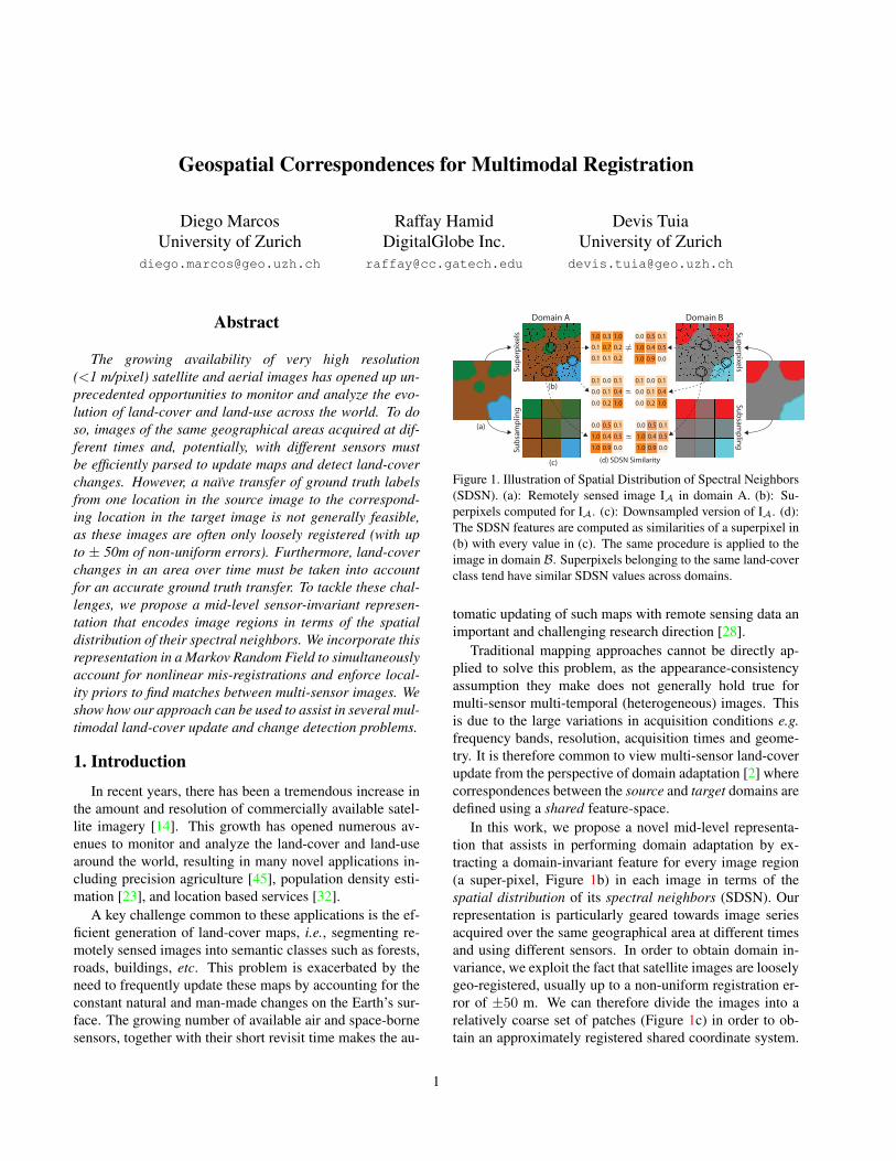
Figure 1. Illustration of Spatial Distribution of Spectral Neighbors
(SDSN). (a): Remotely sensed image IA in domain A. (b): Su-
perpixels computed for IA. (c): Downsampled version of IA. (d):
The SDSN features are computed as similarities of a superpixel in
(b) with every value in (c). The same procedure is applied to the
image in domain B. Superpixels belonging to the same land-cover
class tend have similar SDSN values across domains.
tomatic updating of such maps with remote sensing data an
important and challenging research direction [28].
Traditional mapping approaches cannot be directly ap-
plied to solve this problem, as the appearance-consistency
assumption they make does not generally hold true for
multi-sensor multi-temporal (heterogeneous) images. This
is due to the large variations in acquisition conditions e.g.
frequency bands, resolution, acquisition times and geome-
try. It is therefore common to view multi-sensor land-cover
update from the perspective of domain adaptation [2] where
correspondences between the source and target domains are
defined using a shared feature-space.
In this work, we propose a novel mid-level representa-
tion that assists in performing domain adaptation by ex-
tracting a domain-invariant feature for every image region
(a super-pixel, Figure 1b) in each image in terms of the
spatial distribution of its spectral neighbors (SDSN). Our
representation is particularly geared towards image series
acquired over the same geographical area at different times
and using different sensors. In order to obtain domain in-
variance, we exploit the fact that satellite images are loosely
geo-registered, usually up to a non-uniform registration er-
ror of ±50 m. We can therefore divide the images into a
relatively coarse set of patches (Figure 1c) in order to ob-
tain an approximately registered shared coordinate system.
1

Dom
ain
AD
om
ain
B
a b c d e
HighConfidence
LowConfidence
Figure 2. (a): Remotely sensed images. (b) Superpixel segmenta-
tion of the images. (c): Stack of domain invariant features com-
puted for each superpixel maintaining neighborhood relationships.
(d) Graphical model used to match superpixels from both domains.
(e): Contribution of each match to MRF cost function is used as
confidence map of the matching, enabling the detection of areas
with higher probability of having undergone a land cover change.
By encoding image regions in terms of their spectral dis-
tances from the mean value of each patch in their respec-
tive domains (Figure 1d), SDSN is able to provide a simple
yet effective way to map information across different satel-
lite sensors. This sensor invariance allows to use these fea-
tures for multimodal image registration. We incorporate our
SDSN representation in a Markov Random Field (Figure 2)
where intra-domain edges are used to encourage smooth-
ness and favor matches over short distances, while inter-
domain edges encourage matching superpixels with simi-
lar domain-invariant features (Figure 2d). We show how
this can be used for domain adaptation using two different
strategies: direct transfer of land-cover ground truth (GT)
(§ 4.1) and finding super-pixel pairs for unsupervised mani-
fold alignment (§ 4.2). We also show how this approach can
be used effectively for detecting land-cover changes in an
unsupervised manner (§ 4.3).
2. Related Work
The problem of land-cover segmentation in multi-sensor
and multi-temporal scenarios can be formulated as an in-
stance of the more general problem of domain adaptation,
which addresses the transfer of available domain-specific
knowledge to a different but related domain. Both semi-
supervised [10, 43] and unsupervised [20, 21] approaches
have been proposed to perform domain adaptation.
For semi-supervised approaches, techniques involving
co-training [38], label propagation [44], variants of expec-
tation maximization [9] and SVM [16] have been success-
fully proposed. More recently, approaches involving co-
regularization [26] and data rotation [31] have also been
put forth. These approaches still require few labeled exam-
ples in the target domain, which prevents their application
to problems where such labels are not available.
Unsupervised domain adaptation is generally consid-
ered a harder problem since we do not have any labeled
correspondence between the domains. In this regard, ap-
proaches relying on source-target partial distribution simi-
larity [19], clustering [35, 24, 7], structural correspondence
learning [6], domain divergence minimization [5], manifold
alignment [42] and deep learning [17] have been proposed.
However, these methods require a certain level of corre-
lation between the distributions of both domains. In this
work, we put forth a strategy that is able to deal with dis-
tributions from different domains without requiring them to
be correlated by exploiting the fact that for our setting the
images are loosely spatially geo-registered.
A third approach, not always explicitly referred to as
domain adaptation, consists of using engineered domain-
invariant features. It has been successfully applied in both
remotely sensed [39, 22] and natural images [27]. Some
of these features (e.g. SIFT [27] or shape descriptors [22])
achieve domain-invariance at the cost of discarding relevant
information, e.g. color in R-G-B imagery, while focusing
only on geometrical information. In contrast, we propose
to fully take into account spectral information while also
offering the possibility to include task-specific appearance
descriptors in the process. SDSN is related to the local self-
similarity (LSS) [33] and global self-similarity (GSS) [11]
features. However, unlike these approaches, SDSN uses ap-
proximate geographical correspondences to allow for cross-
domain comparisons, hence offering both the expressive-
ness of GSS and the simplicity of LSS.
In remote sensing, domain adaptation has been tradition-
ally used for land-cover map update tasks [8, 3]. Most of
these pipelines assume a perfect pixel-to-pixel registration
between multi-temporal images, which is a serious limit-
ing factor for high resolution and multi-sensor data. An
object-based variant resides in the semantic tie points strat-
egy proposed in [30] and used in [29] for remote sensing
domain adaptation. An MRF-based approach [27] signif-
icantly relaxing the co-registration constraint is presented
in [39], where registration and change detection are simul-
taneously performed. They use several correlation similar-
ity measures that imply using the same number of spectral
bands in both domains. Our approach extends this work
to the multi-sensor setting where feature spaces are usually
composed by different types and number of spectral chan-
nels, making it more general.
3. Proposed Method
We use super-pixels as our basic computational unit
since they reduce the size of the problem while offering a
meaningful spatial support. In this work we use the SLIC
segmentation method presented in [1]. Given an image IDof size m × n in domain D, and a SLIC segment size pa-
rameter s, we build a super-pixel image HD of size roughly
(m/s× n/s).We formulate our problem as an object matching prob-
lem by using a Markov Random Field (MRF), similar
to [39, 27]. An important feature of this model is that the
contribution to the MRF energy associated to each matched
pair can be used as an estimate of matching confidence. Ev-
ery super-pixel HjB ∈ HB in domain B (target) is matched
to super-pixel HiA ∈ HA in the domain A (source) with a
certain confidence relative to rest of the matches.
3.1. Spatial Distribution of Spectral Neighbors
Our main hypothesis is that objects that are spectrally
similar in one domain tend to be spectrally similar in other
domains, except when they have undergone a land cover
change. For instance, a patch of vegetation in an RGB im-
age is likely to have a similar color to other areas of vegeta-
tion in that image. At the same time, a patch of vegetation in
a near infrared (NIR) image is likely to look very similar to
other vegetated areas in the same NIR image. This within-
image similarity is independent to how similar or dissimilar
a particular patch of vegetation might look across the two
images. We use this observation to encode each super-pixel
HiD in domain D in terms of its similarity to other regions
of the image (see Figure 1).
To do so, we start by computing a down-scaled version
JD of the original image ID as the average spectral signa-
ture of every non-overlaping d× d patch in ID. Here JD is
of size (m/d× n/d) and contains Q = (mn)/d2 elements.
We then compute the SDSN feature f iSDSN for HiD as:
f iSDSN = [f i1SDSN · · · f iq
SDSN · · · f iQSDSN], (1)
where
f iqSDSN = e−σ‖S(Jq
D)−S(Hi
D)‖2
. (2)
Here, S(JqD) and S(Hi
D) are the spectrum (e.g. RGB color)
associated to JqD and the mean spectrum of Hi
D respectively.
Note that f iSDSN has Q dimensions. Each element f iqSDSN of
f iSDSN encodes the similarity of the spectrum of HiD to the
average spectrum of a particular patch of the image, JqD.
The down-scaling allows for robustness against registration
noise between the images in the different domains. For ex-
ample, a 15 pixel shift in the original image becomes a sub-
pixel shift of 0.15 pixels using downscaling factor of 100.
3.2. Matching Formulation
We build on previous matching approaches relying on
MRF such as [34, 27, 15, 39]. We define a graph G = (V, E)where every edge ǫij ∈ E connects two nodes i, j ∈ V with
a weight c(ǫij). Every node i corresponds to a super-pixel
HiB in the target domain. Since we expect the misregis-
tration shifts to be consistent within a region of the image,
possibly with shift larger than the superpixel size, we con-
sider mid-range connections for node i, Ni, beyond first or-
der neighborhoods. In our experiments (Section 4) we use
a 25 × 25 super-pixel neighborhood. We make use of the
SLIC grid initialization to define the neighborhood systems
efficiently. We set weights c(ǫij) inversely proportional to
the geographical distance between node i and its neighbors
and we normalize them such that∑
ǫij∈Nic(ǫij) = 1. Each
node is defined by its geographical coordinates pi = (x, y)and is assigned to a matching vector wi = (u, v) towards
a super-pixel Mi = HkA in the source domain, defined by
its coordinates qk = pi + wi. M is a look-up table stor-
ing the currently selected matches. The matching process is
formulated as an energy minimization over the graph G as:
E(M) =∑
i
Θdata(HiB, H
kA) + λsmall
∑
i
Φsmall(wi)
+ λsmooth
∑
i
Φsmooth(Ni). (3)
The data term Θdata measures the dissimilarity between
HiB and its match Hk
A, defined by:
Θdata =∑
f∈F
αfΘf (4)
where αf is the weight given to each dissimilarity measure
Θf , computed using the feature f , e.g. SDSN, SIFT, color,
etc. Here F defines the set of all features considered.
The dissimilarity between a pair of superpixels HkA and
HjB in feature f ∈ F is computed as:
Θf (HkA, H
iB) = −log
(
f(HkA)
⊤ · f(HiB))
(5)
We normalize each feature to have unit ℓ2-norm. To further
spread the samples over the unit ball, we center every vector
to zero mean. Note that the matrix version of this formula-
tion can use optimized BLAS Level-3 [18] and therefore
can be computed efficiently by optimally using all the re-
sources of modern computing architecture.
In Equation (3), the term Φsmall penalizes big matching
displacements and depends only on the matching vector:
Φsmall(i) = ‖wi‖2 (6)
Similarly, Φsmooth penalizes matching vectors deviating too
much from the average matching vector in a neighborhood:
Φsmooth(Ni) = ‖wi −∑
j∈Ni
c(ǫij)wj‖2 (7)
where all j ∈ Ni are the neighbors of i and each ǫij the
corresponding edge, with c(ǫij) being the edge weight.
The confidence of the match of node i in the target do-
main B is then defined as −E(Mi).
3.3. Optimization
Since satellite images are loosely pre-aligned, the opti-
mal solution does not have large w. Therefore, we limit
the search for a match for i ∈ B to a window of size

w × w around the initial match. In practice, we initial-
ize the system on the geographically nearest super-pixel in
A. Note that we can see the matching problem as a clas-
sification problem with w2 classes, corresponding to every
possible match for each super-pixel in B[15]. To find a set
of matches M that minimize Equation (3), we employ the
Iterated Conditional Modes (ICM) algorithm [4]. Thanks
to the grid structure of the graph we can use Fast Fourier
Transform (FFT) to compute the energy in the form of a
convolution, which significantly improves the efficiency of
the algorithm. The fact that the initialization is never very
far from the solution [37], the use of super-pixels and the
FFT means that, for images pairs used in this work, the pre-
sented method typically converges in less than 10 seconds
using ICM on a standard personal computer.
4. Experiments and Results
We apply our proposed representation to 3 different
problems within the context of multimodal registration. In
all the experiments the SDSN feature is compared to a
multi-scale SIFT feature over the average color channel
with patch sizes of 9, 17 and 33 pixels [40] and a feature
consisting of the common spectral bands, thereafter referred
to as “color”. In all the experiments using a set of 2 features,
the values of αf have been set to 0.5.
4.1. Ground Truth Transfer
We aim to transfer the available ground truth (GT) from
the source image to the target image, while simultaneously
avoiding the regions that have likely undergone some land
cover change. This transferred GT is then used to train a
kNN classifier in the target domain to generate an updated
land cover map. The choice of kNN classifier is due to its
simplicity and distribution independence. We use a hand la-
beled GT of the target domain to validate the map obtained.
4.1.1 Dataset and Setup
The source domain consists of five QuickBird [12] satellite
images of Zurich Switzerland taken in August 2002. They
have four channels: near infrared, red, green and blue (NIR-
R-G-B), and a resolution of about 0.62 cm/pixel. These im-
age are a subset of the Zurich Summer dataset presented
in [41]. The target domain is a corresponding set of five
NIR-R-G aerial images of the same area, with nearly the
same footprint, captured during the campaign of summer
2013 and provided by the Swiss Federal Office of Topogra-
phy [36]. We refer to this dataset as NIR-R-G Orthophoto
data. The resolution of the target images is 25 cm/pixel.
To test our approach in the case where source and target
only share the R and G bands, we discard the NIR band
of the QuickBird images and use exclusively the R-G-B
(a) (b)Figure 3. One of the 5 image pairs from the Zurich dataset. (a)
Quickbird [12] image, the source domain, and the correspond-
ing GT. (b) False color Representation of the 3 band NIR-R-G
Orthophoto data [36] (2013) and its GT: Roads, buildings, trees,
grass, water and bare soil. Best viewed in color.
bands throughout the experiments. Figure 3 shows an ex-
ample image pair and the corresponding GT maps. In this
dataset, the geo-registration error of the image pairs ranges
from 5 m to 15 m. Each image in the source domain has a
quite dense GT land-cover map consisting of between four
and six classes among Roads, Buildings, Trees, Grass, Bare
Soil, Water, Railways and Swimming Pools.
We treat each of the five image pairs as an independent
GT transfer problem. For each image pair, we first re-scale
them to the size of the smaller image in the pair. Note that
this step is not required but it results in obtaining a similar
number of superpixels, which helps getting a good match-
ing. The images are then segmented with SLIC [1], with the
superpixel size of 10 pixels and the regularization parame-
ter values set to 10. The SDSN features are computed using
a downsampling factor d of 20 and a σ of 0.5. For the MRF
matching, we used λsmooth = 0.05 and λsmall = 0.05.
After matching, 90% most confident matches are used
for transferring the GT to the target image. We then used
all the transferred GT to train a pixel-wise kNN classifier
with k = 5. The classified land cover map is compared to
the hand labeled target GT for validation. We report results
from QuickBird [12] to Orthophoto [36] and vice versa.
4.1.2 Results
The classification results are shown in in Table 1. Using
SIFT or color features alone produces results that are signif-
icantly worse than the results obtained using the proposed
SDSN features. Using SDSN in conjunction with SIFT pro-
duces the best results on average. This is because SDSN and
SIFT encode very different properties of the super-pixels,

i.e., the former encodes spectral information in terms of
global interactions across the whole image, while the lat-
ter encodes the local geometry. These two forms of in-
formation complement each other in describing land-cover
changes, resulting in better GT transfer. We also compare
our results with those obtained using a multi-modal mutual
information-based registration method [25] (Table 2).
#Transfer
Dir.Color SIFT
Color
+SIFTSDSN
SDSN
+SIFT
SDSN
+Color
1A → B 0.652 0.551 0.579 0.694 0.716 0.678
B → A 0.281 0.438 0.371 0.548 0.572 0.414
2A → B 0.665 0.629 0.678 0.684 0.690 0.681
B → A 0.396 0.510 0.475 0.536 0.541 0.466
3A → B 0.711 0.714 0.705 0.731 0.749 0.733
B → A 0.538 0.582 0.561 0.561 0.584 0.563
4A → B 0.585 0.644 0.551 0.730 0.694 0.597
B → A 0.453 0.548 0.484 0.498 0.557 0.480
5A → B 0.559 0.766 0.756 0.782 0.790 0.786
B → A 0.599 0.690 0.705 0.723 0.711 0.720
Mean 0.544 0.607 0.586 0.649 0.660 0.612
Table 1. Average classification accuracy for ground truth transfer.
The first column correspond to image pairs. A and B correspond
to QuickBird [12] Orthophoto [36] domains.
Method SDSN+SIFT Affine[25] Non-rigid[25]
AA 66.0% 63.7% 64.0%
Table 2. Numerical comparison with [25], Average Accuracy.
4.1.3 Parameter Sensitivity and Circular Validation
We now focus on the sensitivity of our method to the choice
of parameter values used when transferring the GT from
source to target A → B. In the left column of Figure 4 we
see the result of applying this concept to the values of λsmall
and λsmooth, the SDSN’s σ, and the down-scaling factor d.
It can be observed that that most image-pairs are not very
sensitive to variations in the tested parameters showing the
robustness of our framework to its various parameters.
We also study how a circular validation strategy [7] can
help in estimating a good set of parameters for our frame-
work. In the case of GT transfer, this can be done by trans-
ferring the GT from source to target A → B, and then from
target back to source A → B → A, where it is compared
to the original GT for evaluation. This setting corresponds
to the right column of Figure 4. It can be observed that the
optimal values obtained during validation A → B → A are
similar to the optimal values required for our original prob-
lem A → B. This result shows that we can employ this
circular validation strategy [7] in practice to select the opti-
mal parameter values required by our framework. Note that
λsmall
and λsmooth
10 -2 10 -1 10 0
Ave
rage
Acc
urac
y
0.2
0.4
0.6
0.8
A → B
1
2
3
4
5
λsmall
and λsmooth
10 -2 10 -1 10 0
Ave
rage
Acc
urac
y
0.2
0.4
0.6
0.8
A → B → A
(a)
SDSN σ
0.5 1 1.5
Ave
rage
Acc
urac
y
0.2
0.4
0.6
0.8
A → B
SDSN σ
0.5 1 1.5
Ave
rage
Acc
urac
y
0.2
0.4
0.6
0.8
A → B → A
(b)
Downsampling parameter, d
50 100 150
Ave
rag
e A
ccu
racy
0.2
0.4
0.6
0.8
A → B
Downsampling parameter, d
50 100 150
Ave
rag
e A
ccu
racy
0.2
0.4
0.6
0.8
A → B → A
(c)Figure 4. Classification accuracy in the five Zurich image pairs for
different values of (a): λsmall and λsmooth (both take the same value
in this experiment), (b): σ value for the SDSN feature, (c) the
downscaling parameter d for the SDSN feature. On the left, we
transfer the GT from source to target. On the right is from source
to target and back to source.
the downsampling factor d determines the number of op-
eration required to compute the SDSN feature and effects
the computation time in a quadratic manner (see Table 3).
However, the results in Figure 4 suggest that this time can
be greatly reduced at a small cost in accuracy.
d 2 5 10 20 50 100
time (s) 4.71 0.75 0.255 0.073 0.04 0.04
Table 3. Time (images 700 × 1000 pixels on a single CPU) to
compute SDSN features wrt. downsampling, d.
4.1.4 Sensitivity to Perturbations in the Input
We use the image shown in Figure 3a in order to explore
how sensitive our method is to three types of perturbations:
1) amount of change, 2) displacement and 3) rotation be-
tween the images. To do so, we match the image in Fig-
ure 3a and a perturbed version of itself. The land-cover
changes were added by substituting vegetation superpixels

(a) (b) (c)Figure 5. (a): Layout of the used images in the area of Lausanne, Switzerland. (b): Representation of the 2 images used (left) and the
respective GTs (right). From top to bottom: Prilly 2011 (WorldView 2 [13]) and Renens 2012 (NIR-R-G Orthophoto). Color legend:
buildings, roads, grass, trees and shadows. (c): Hand labeled super-pixel pairs (in yellow). Figure best viewed in color.
with bare soil ones. Performance was measured as the per-
centage of changed superpixels recalled, assuming that the
amount of change had been correctly estimated. When con-
sidering displacement and rotation, the amount of change is
fixed at 20%. Results in Table 4 show high robustness even
for the most extreme amounts of change and displacement,
which are the main sources of perturbation to be expected
in remotely sensed images.
Change amount (%) 6 12 30 42
Recall (%) 96 97 96 84
Displacement (m) 10 20 30 50
Recall (%) 92 86 85 82
Angle (◦) 1 3 6 10
Recall (%) 89 78 62 57
Table 4. Sensitivity to changes, displacements and rotations in the
target (B). Domains A and B consist of the RBG and NIR-R-G
bands of Figure 3a respectively.
4.2. Unsupervised Manifold Alignment
We now explore the problem where the source and target
images have a partial overlap, but there is no GT available
in the overlap area. To perform domain adaptation, we can-
not simply register the labeled super-pixels directly. How-
ever, we can project both domains in a common latent space
where both domains are similarly distributed. We use the
same settings presented in [29], where a hand-labeled set
of super-pixel pairs in the overlapping area are used to per-
form manifold alignment between the two domains. Instead
of manual selection however, we use the proposed method
to automatically find a set of these super-pixel pairs.
We use the manifold alignment algorithm in [43], where
the local geometrical structure of the domain is preserved
while enforcing weak class consistency using the matched
super-pixel pairs. Once the domains are aligned, one can
then directly train and test in the aligned domain.
To find a set of confident super-pixel matches that are
also representative of the different land covers in the im-
age, we partition the super-pixel spectra in the target do-
main using k-means clustering and select the most confident
matches in each cluster.
(a) (b)Figure 6. Automatically generated super-pixel pair map using the
proposed SDSN features. (a) Grayscale version of the World-View
2 [13] image used as source. (b) Grayscale version of the NIR-R-G
Orthophoto [36] image used as target. Matched segment pairs are
within the neighborhood of each other and are marked with same
color in order to imply correspondence. Best viewed in color.
4.2.1 Dataset and Setup
For these experiments, we use the dataset presented in [29].
The images cover an area of Lausanne, Switzerland. The
source domain is a WorldView 2 [13] image, with 8 spec-
tral bands in the visible and infrared region, taken in 2011and the target domain is a 25 cm/pixel resolution NIR-R-G
Orthophoto [36]. Figure 5b shows the areas of interest, with
their corresponding GT, and Figure 5c the area common
to both domains. The land-cover classification includes 5classes, as shown in Figure 5b.
The parameters for SLIC were set to segment size of
20 pixels and regularization parameter of 10. The σ value
for the SDSN was set to 0.5 and the downsampling factor
for the low resolution image was set to 100. For the MRF
matching, we used λsmooth = 10−2 and λsmall = 10−2. We
then partitioned the superpixels in the target domain into 26
clusters and randomly took 10 confident matches from each
of the 20 most populated clusters.
For manifold alignment, we used the same settings as
in [29]. After projecting the data onto the latent feature
space, we tested the performance of the alignment by clas-
sifying in the test image using only the labeled pixels from
the source image. We report results using kNN with k = 5training with 400 labeled pixels per class. We also tried
other classifiers, such as Random Forest and SVM (not
shown in this paper), obtaining comparable trends. For
each type of feature (color, SIFT, SDSN and SDSN+SIFT)
we generated 5 instances of super-pixel pair set. For each
instance, as well as for the hand labeled super-pixel pairs,
we computed 10 realizations of the manifold alignment and
classification training set.
# of dimensions used in the latent space
2 4 6 8 10 12
Ove
rall
accu
racy,
%
40
45
50
55
60
65
70
75
80
85
90
95KNN
SDSN
color
SIFT
SDSN+SIFT
hand labeled
train on source
train on target
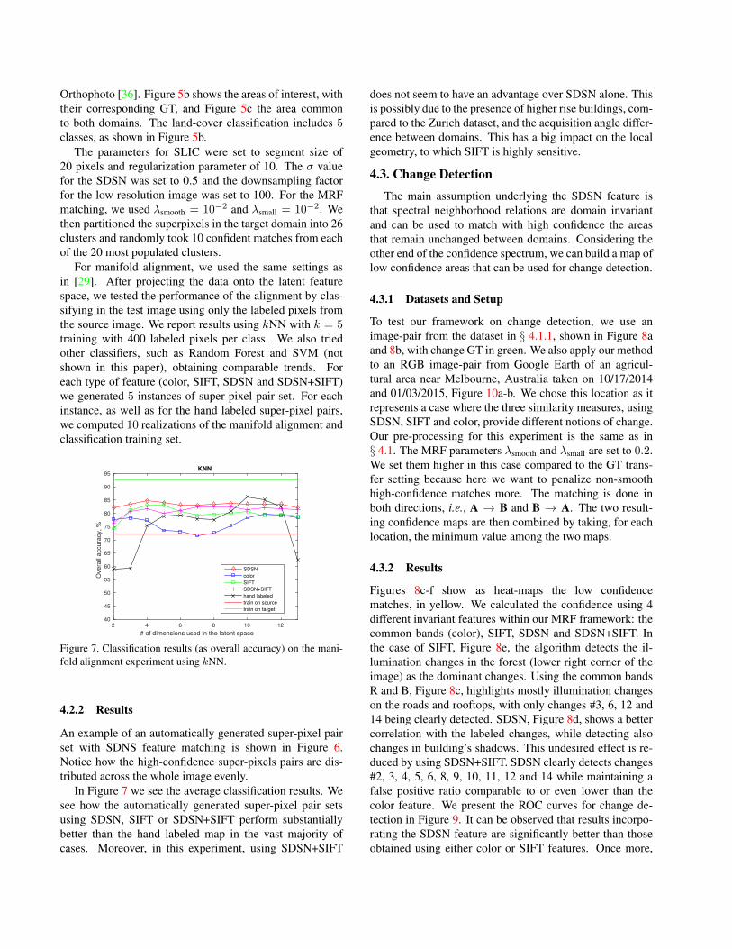
Figure 7. Classification results (as overall accuracy) on the mani-
fold alignment experiment using kNN.
4.2.2 Results
An example of an automatically generated super-pixel pair
set with SDNS feature matching is shown in Figure 6.
Notice how the high-confidence super-pixels pairs are dis-
tributed across the whole image evenly.
In Figure 7 we see the average classification results. We
see how the automatically generated super-pixel pair sets
using SDSN, SIFT or SDSN+SIFT perform substantially
better than the hand labeled map in the vast majority of
cases. Moreover, in this experiment, using SDSN+SIFT
does not seem to have an advantage over SDSN alone. This
is possibly due to the presence of higher rise buildings, com-
pared to the Zurich dataset, and the acquisition angle differ-
ence between domains. This has a big impact on the local
geometry, to which SIFT is highly sensitive.
4.3. Change Detection
The main assumption underlying the SDSN feature is
that spectral neighborhood relations are domain invariant
and can be used to match with high confidence the areas
that remain unchanged between domains. Considering the
other end of the confidence spectrum, we can build a map of
low confidence areas that can be used for change detection.
4.3.1 Datasets and Setup
To test our framework on change detection, we use an
image-pair from the dataset in § 4.1.1, shown in Figure 8a
and 8b, with change GT in green. We also apply our method
to an RGB image-pair from Google Earth of an agricul-
tural area near Melbourne, Australia taken on 10/17/2014
and 01/03/2015, Figure 10a-b. We chose this location as it
represents a case where the three similarity measures, using
SDSN, SIFT and color, provide different notions of change.
Our pre-processing for this experiment is the same as in
§ 4.1. The MRF parameters λsmooth and λsmall are set to 0.2.
We set them higher in this case compared to the GT trans-
fer setting because here we want to penalize non-smooth
high-confidence matches more. The matching is done in
both directions, i.e., A → B and B → A. The two result-
ing confidence maps are then combined by taking, for each
location, the minimum value among the two maps.
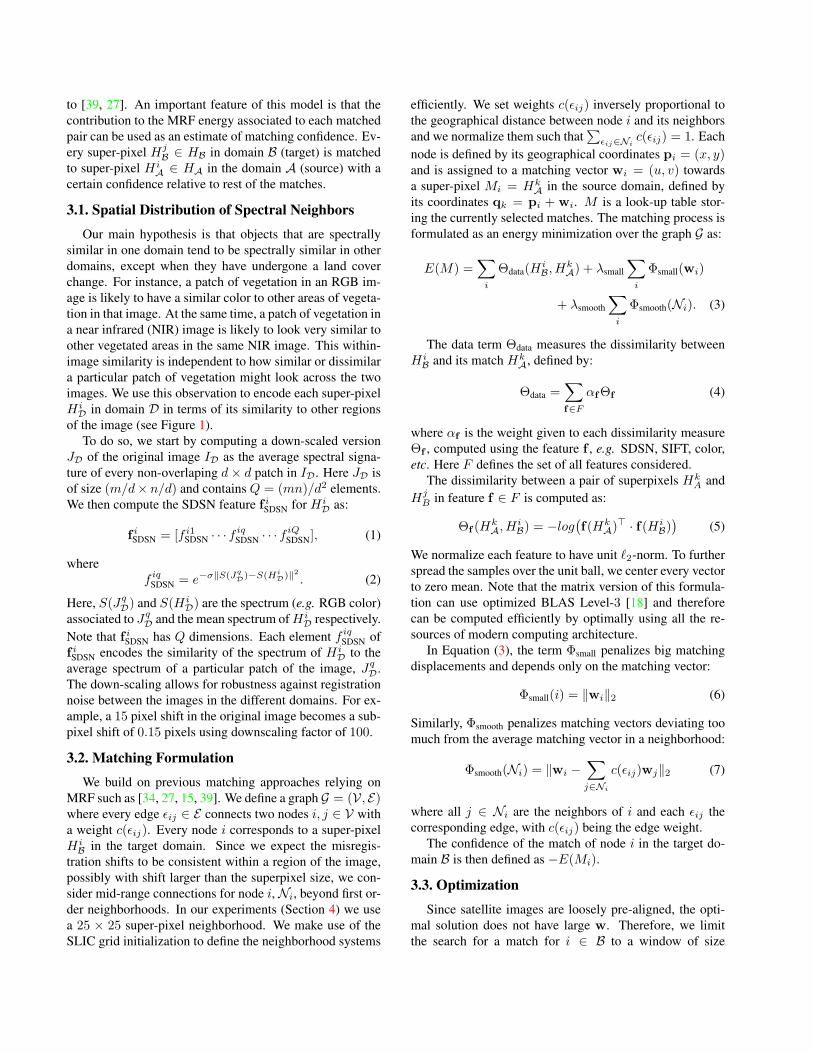
4.3.2 Results
Figures 8c-f show as heat-maps the low confidence
matches, in yellow. We calculated the confidence using 4
different invariant features within our MRF framework: the
common bands (color), SIFT, SDSN and SDSN+SIFT. In
the case of SIFT, Figure 8e, the algorithm detects the il-
lumination changes in the forest (lower right corner of the
image) as the dominant changes. Using the common bands
R and B, Figure 8c, highlights mostly illumination changes
on the roads and rooftops, with only changes #3, 6, 12 and
14 being clearly detected. SDSN, Figure 8d, shows a better
correlation with the labeled changes, while detecting also
changes in building’s shadows. This undesired effect is re-
duced by using SDSN+SIFT. SDSN clearly detects changes
#2, 3, 4, 5, 6, 8, 9, 10, 11, 12 and 14 while maintaining a
false positive ratio comparable to or even lower than the
color feature. We present the ROC curves for change de-
tection in Figure 9. It can be observed that results incorpo-
rating the SDSN feature are significantly better than those
obtained using either color or SIFT features. Once more,
(a) (b)
(c) (d)
(e) (f)Figure 8. (a) Image in domain A and (b) B. Change GT marked
in green. (c-f) The low confidence areas, those contributing the
most to the MRF energy, are shown in yellow. The matching has
been performed with the same parameters using the following fea-
tures: (a) common spectral bands, (b) SIFT , (c) SDSN and (d)
SDSN+SIFT. Best viwed in color.
False positives
0 0.2 0.4 0.6 0.8 1
Tru
e p
ositiv
es
0
0.2
0.4
0.6
0.8
1
Color
SIFT
SDSN
SDSN+SIFT
Figure 9. Correctly detected change pixels versus false positives
for all different values of the detection threshold.
using SDSN+SIFT results in a slightly better performance
than SDSN alone.
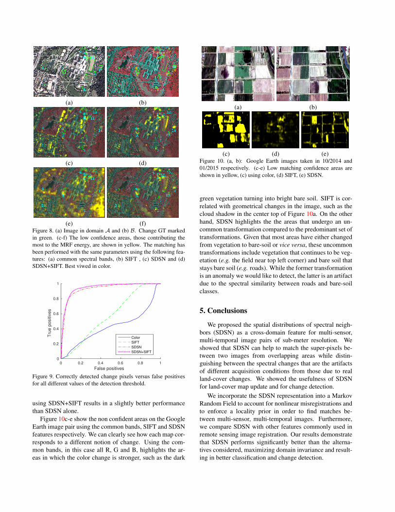
Figure 10c-e show the non confident areas on the Google
Earth image pair using the common bands, SIFT and SDSN
features respectively. We can clearly see how each map cor-
responds to a different notion of change. Using the com-
mon bands, in this case all R, G and B, highlights the ar-
eas in which the color change is stronger, such as the dark
(a) (b)
(c) (d) (e)Figure 10. (a, b): Google Earth images taken in 10/2014 and
01/2015 respectively. (c-e) Low matching confidence areas are
shown in yellow, (c) using color, (d) SIFT, (e) SDSN.
green vegetation turning into bright bare soil. SIFT is cor-
related with geometrical changes in the image, such as the
cloud shadow in the center top of Figure 10a. On the other
hand, SDSN highlights the the areas that undergo an un-
common transformation compared to the predominant set of
transformations. Given that most areas have either changed
from vegetation to bare-soil or vice versa, these uncommon
transformations include vegetation that continues to be veg-
etation (e.g. the field near top left corner) and bare soil that
stays bare soil (e.g. roads). While the former transformation
is an anomaly we would like to detect, the latter is an artifact
due to the spectral similarity between roads and bare-soil
classes.
5. Conclusions
We proposed the spatial distributions of spectral neigh-
bors (SDSN) as a cross-domain feature for multi-sensor,
multi-temporal image pairs of sub-meter resolution. We
showed that SDSN can help to match the super-pixels be-
tween two images from overlapping areas while distin-
guishing between the spectral changes that are the artifacts
of different acquisition conditions from those due to real
land-cover changes. We showed the usefulness of SDSN
for land-cover map update and for change detection.
We incorporate the SDSN representation into a Markov
Random Field to account for nonlinear misregistrations and
to enforce a locality prior in order to find matches be-
tween multi-sensor, multi-temporal images. Furthermore,
we compare SDSN with other features commonly used in
remote sensing image registration. Our results demonstrate
that SDSN performs significantly better than the alterna-
tives considered, maximizing domain invariance and result-
ing in better classification and change detection.
References
[1] R. Achanta, A. Shaji, K. Smith, A. Lucchi, P. Fua, and
S. Susstrunk. Slic superpixels compared to state-of-the-art
superpixel methods. IEEE Transactions on Pattern Analysis
and Machine Intelligence, 34(11):2274–2282, Nov 2012. 2,
4
[2] S. Ben-David, J. Blitzer, K. Crammer, A. Kulesza, F. Pereira,
and J. W. Vaughan. A theory of learning from different do-
mains. Machine learning, 79(1-2):151–175, 2010. 1
[3] C. Benedek and T. Sziranyi. Change detection in opti-
cal aerial images by a multilayer conditional mixed Markov
model. IEEE Transactions on Geoscience and Remote Sens-
ing, 47(10):3416–3430, 2009. 2
[4] J. Besag. On the statistical analysis of dirty pictures. Journal
of the Royal Statistical Society. Series B (Methodological),
pages 259–302, 1986. 4
[5] J. Blitzer, K. Crammer, A. Kulesza, F. Pereira, and J. Wort-
man. Learning bounds for domain adaptation. In Advances
in neural information processing systems, pages 129–136,
2008. 2
[6] J. Blitzer, M. Dredze, F. Pereira, et al. Biographies, bol-
lywood, boom-boxes and blenders: Domain adaptation for
sentiment classification. In ACL, volume 7, pages 440–447,
2007. 2
[7] L. Bruzzone and M. Marconcini. Domain adaptation prob-
lems: A DASVM classification technique and a circular val-
idation strategy. IEEE Transactions on Pattern Analysis and
Machine Intelligence, 32(5):770–787, 2010. 2, 5
[8] L. Bruzzone and S. B. Serpico. An iterative technique for the
detection of land-cover transitions in multitemporal remote-
sensing images. IEEE Transactions on Geoscience and Re-
mote Sensing, 35(4):858–867, 1997. 2
[9] W. Dai, G.-R. Xue, Q. Yang, and Y. Yu. Transferring naive
bayes classifiers for text classification. In Proceedings of the
National Conference on Artificial Intelligence, volume 22,
page 540. Menlo Park, CA; Cambridge, MA; London; AAAI
Press; MIT Press; 1999, 2007. 2
[10] H. Daume III and D. Marcu. Domain adaptation for statis-
tical classifiers. Journal of Artificial Intelligence Research,
pages 101–126, 2006. 2
[11] T. Deselaers and V. Ferrari. Global and efficient self-
similarity for object classification and detection. In Com-
puter Vision and Pattern Recognition (CVPR), 2010 IEEE
Conference on, pages 1633–1640. IEEE, 2010. 2
[12] DigitalGlobe. QuickBird datasheet. http:
//global.digitalglobe.com/sites/default/
files/QuickBird-DS-QB-Prod.pdf/, 2000. 4, 5
[13] DigitalGlobe. WorldView 2 datasheet. http:
//global.digitalglobe.com/sites/default/
files/DG_WorldView2_DS_PROD.pdf/, 2000. 6
[14] J. Doe. Commercial satellite imaging market - global indus-
try analysis, size, share, growth, trends, and forecast, 2013 -
2019. Transparency Market Research, 2014. 1
[15] P. S. Dragomir Anguelov, H.-C. Pang, D. Koller, and J. D.
Sebastian Thrun. The correlated correspondence algorithm
for unsupervised registration of nonrigid surfaces. In Ad-
vances in Neural Information Processing Systems 17: Pro-
ceedings of the 2004 Conference, volume 17, page 33. MIT
Press, 2005. 3, 4
[16] L. Duan, I. W. Tsang, D. Xu, and T.-S. Chua. Domain
adaptation from multiple sources via auxiliary classifiers. In
Proceedings of the 26th Annual International Conference on
Machine Learning, pages 289–296. ACM, 2009. 2
[17] Y. Ganin and V. Lempitsky. Unsupervised domain adaptation
by backpropagation. arXiv preprint arXiv:1409.7495, 2014.
2
[18] G. H. Golub and C. F. Van Loan. Matrix computations, vol-
ume 3. JHU Press, 2012. 3
[19] B. Gong, K. Grauman, and F. Sha. Connecting the dots with
landmarks: Discriminatively learning domain-invariant fea-
tures for unsupervised domain adaptation. In Proceedings
of The 30th International Conference on Machine Learning,
pages 222–230, 2013. 2
[20] B. Gong, Y. Shi, F. Sha, and K. Grauman. Geodesic flow ker-
nel for unsupervised domain adaptation. In Computer Vision
and Pattern Recognition (CVPR), 2012 IEEE Conference on,
pages 2066–2073. IEEE, 2012. 2
[21] R. Gopalan, R. Li, and R. Chellappa. Domain adaptation
for object recognition: An unsupervised approach. In Com-
puter Vision (ICCV), 2011 IEEE International Conference
on, pages 999–1006. IEEE, 2011. 2
[22] L. Gueguen and R. Hamid. Large-scale damage detection
using satellite imagery. In Proceedings of the IEEE Con-
ference on Computer Vision and Pattern Recognition, pages
1321–1328, 2015. 2
[23] J. Harvey. Estimating census district populations from satel-
lite imagery: some approaches and limitations. International
Journal of Remote Sensing, 23(10):2071–2095, 2002. 1
[24] N. Japkowicz and S. Stephen. The class imbalance problem:
A systematic study. Intelligent data analysis, 6(5):429–449,
2002. 2
[25] D.-J. Kroon and C. H. Slump. MRI modality transformation
in demon registration. In Proc. ISBI, pages 963–966, 2009.
5
[26] A. Kumar, A. Saha, and H. Daume. Co-regularization based
semi-supervised domain adaptation. In Advances in neural
information processing systems, pages 478–486, 2010. 2
[27] C. Liu, J. Yuen, and A. Torralba. SIFT flow: Dense
correspondence across scenes and its applications. IEEE
Transactions on Pattern Analysis and Machine Intelligence,
33(5):978–994, 2011. 2, 3
[28] D. Lu, G. Li, and E. Moran. Current situation and needs of
change detection techniques. International Journal of Image
and Data Fusion, 5(1):13–38, 2014. 1
[29] D. Marcos-Gonzalez, G. Camps-Valls, and D. Tuia. Weakly
supervised alignment of multisensor images. In Geoscience
and Remote Sensing Symposium (IGARSS), July 2015. 2, 6,
7
[30] J. Montoya-Zegarra, C. Leistner, K. Schindler, et al. Seman-
tic tie points. In Applications of Computer Vision (WACV),
2013 IEEE Workshop on, pages 377–384. IEEE, 2013. 2
[31] S. J. Pan, I. W. Tsang, J. T. Kwok, and Q. Yang. Domain
adaptation via transfer component analysis. IEEE Transac-
tions on Neural Networks, 22(2):199–210, 2011. 2
[32] J. Schiller and A. Voisard. Location-based services. Elsevier,
2004. 1
[33] E. Shechtman and M. Irani. Matching local self-similarities
across images and videos. In Computer Vision and Pattern
Recognition, 2007. CVPR’07. IEEE Conference on, pages 1–
8. IEEE, 2007. 2
[34] A. Shekhovtsov, I. Kovtun, and V. Hlavac. Efficient mrf de-
formation model for non-rigid image matching. Computer
Vision and Image Understanding, 112(1):91–99, 2008. 3
[35] H. Shimodaira. Improving predictive inference under covari-
ate shift by weighting the log-likelihood function. Journal of
statistical planning and inference, 90(2):227–244, 2000. 2
[36] Swisstopo. Swiss Federal Office of Topography SWIS-
SIMAGE FCIR. http://www.swisstopo.admin.
ch/internet/swisstopo/en/home/products/
images/ortho/swissimage/SWISSIMAGE_FCIR.
html. 4, 5, 6, 7
[37] R. Szeliski, R. Zabih, D. Scharstein, O. Veksler, V. Kol-
mogorov, A. Agarwala, M. Tappen, and C. Rother. A com-
parative study of energy minimization methods for Markov
Random Fields. In Computer Vision–ECCV 2006, pages 16–
29. Springer, 2006. 4
[38] G. Tur. Co-adaptation: Adaptive co-training for semi-
supervised learning. In IEEE International Conference on
Acoustics, Speech and Signal Processing, pages 3721–3724.
IEEE, 2009. 2
[39] M. Vakalopoulou, K. Karantzalos, N. Komodakis, and
N. Paragios. Simultaneous registration and change detection
in multitemporal, very high resolution remote sensing data.
In Proceedings of the IEEE Conference on Computer Vision
and Pattern Recognition Workshops, pages 61–69, 2015. 2,
3
[40] A. Vedaldi and B. Fulkerson. VLFeat: An open and portable
library of computer vision algorithms. http://www.
vlfeat.org/, 2008. 4
[41] M. Volpi and V. Ferrari. Semantic segmentation of urban
scenes by learning local class interactions. In Proceedings
of the IEEE Conference on Computer Vision and Pattern
Recognition Workshops, pages 1–9, 2015. 4
[42] C. Wang and S. Mahadevan. Manifold alignment without
correspondence. In IJCAI, volume 2, page 3, 2009. 2
[43] C. Wang and S. Mahadevan. Heterogeneous domain adap-
tation using manifold alignment. In IJCAI Proceedings-
International Joint Conference on Artificial Intelligence, vol-
ume 22, page 1541, 2011. 2, 6
[44] D. Xing, W. Dai, G.-R. Xue, and Y. Yu. Bridged refinement
for transfer learning. In Knowledge Discovery in Databases:
PKDD 2007, pages 324–335. Springer, 2007. 2
[45] C. Yang, J. H. Everitt, Q. Du, B. Luo, and J. Chanussot. Us-
ing high-resolution airborne and satellite imagery to assess
crop growth and yield variability for precision agriculture.
Proceedings of the IEEE, 101(3):582–592, 2013. 1