georgetown public policy review volume 17 1 graduate thesis edition 2011-2012

GeorGetown public policy review | i

Graduate thesis edition

Editor’s Remarks

Research

Unlocking the American Dream: Exploring Intergenerational Social Mobility and the Persistence of Economic Status in the United StatesDavid P. Cooper ....................................................................................................... 1

Armed Conflict and Early Childhood Outcomes in Ethiopia and PerúKate Anderson Simons ........................................................................................... 43

Politics of Enforcement: How the Department of Justice Enforces the Civil False Claims ActR. Brent Wisner ...................................................................................................... 61

The Academic Achievement of First and Second Generation Immigrants in the United StatesEmilie C. Saleh ....................................................................................................... 71

Malaria Prevention in Liberian Children: Impacts of Bed Net Ownership and Use Yasmein Asi ............................................................................................................ 77

Interview

An Interview with Donald Marron, Director of the Tax Policy CenterKathryn Short ........................................................................................................ 95

GeorGetown public policy review | iii

Editor-in-Chief Amanda Huffman

Executive Managing Editor richard Harris

Executive Print Editor Kathryn bailey

Executive Online Editor luca etter

Executive Interview Editor Kathryn Short

Executive Director, christina Moore Marketing & Outreach

Executive Director, Matthew Doyle Graduate Thesis Edition

Executive Director, Jennie Herriot Hatfield Finance and Operations

Executive Director, Sarah orzell Data and Analytics

Senior Marketing Director, Kaitlin ritchey Events & Fundraising

Senior Marketing Directors, Kim peyser, Jason bowles Policy Forums

Senior Marketing Director, Ashley nichols Alumni Relations

Associate Marketing Director long Hong

Senior Print Editors Allison Johnson, Danielle parnass, Michelle wein

Associate Print Editors betsy Keating, lauren Shaw, thomas Smith, Malek Abu-Jawdeh, chris Adams, noora Al Sindi, Adina Appelbaum, Jason clark, Ana Maria Diaz, Kim Dancy, paul Heberling, robbie Johnson, long Hong

Copy Editors isabel taylor, Maya Khan, Mark Sharoff, Jason Kumar, carl Ginther, robbie Johnson, Malek Abu-Jawdeh

Senior Interview Editors ingrid Stegemoeller, robert wood

Senior Online Editors rose tutera-baldauf, isabel taylor, Amir Fouad, Joe cox, Sarah larson, Kate rosenberg

Associate Online Editors Josh Caplan, Amy Costanzo, David Dickey-Griffith, Aaron Dimmick, Alex engler, chris Hildebrand, Jason Kumar, Henry Schleifer, rob Stone, Mark Sharoff, erin ingraham, Maya Khan,

Associate Online Writers christopher Klein, noora Al Sindi

Faculty Advisor robert bednarzik

Thesis Advisors robert bednarzik, Adam thomas, Andreas Kern, Andrew wise, Gillette Hall

Special Thanks We would like to express our infinite gratitude to Darlene Brown, Felecia langford, e.J. Dionne, paul begala, ward Kay, lynn ross, Mark rom, barbara Schone, ed Montgomery, and the Georgetown public policy institute

Cover Design www.acecreative.biz

Interior Design & Layout Amanda Huffman

Printer print 1 printing & copying

iv | GenerAl inForMAtion

The Georgetown Public Policy Review publishes articles that contribute to the thoughtful discourse of public policy. The Graduate Thesis Edition is reserved for those thesis papers of Georgetown Public Policy Insitute alumni that showcase superior policy analysis and thoughtful writing. To be included in The Review, each author must be nominated by a GPPI professor and take part in a comprehensive review process led by Review staff members. For more information about the Graduate Thesis Edition, visit www.gppreview.com.

INSTRUCTIONS FOR CONTRIBUTORS The Georgetown Public Policy Review receives a large quantity of submissions for every issue, which may alter our schedule by a couple of months. You may email a letter of inquiry about our upcoming theme or look us up online. Articles should be original and must not draw substantially from previously published works by the author. No simultaneous submissions please. Commentaries, opinion articles and essays should be under 3,000 words. Research articles can be between 3,000 and 5,000 words. All articles must utilize the accepted tools of policy analysis. We do consider longer pieces, but include only one such piece in a given issue. Adhere to the format in The Chicago Manual of Style.

Articles can be submitted by email ([email protected]) or posted to our address. Submissions should include one cover document containing contact information (author’s name, address, telephone and email address). Please indicate the primary contact if there are multiple authors. Do not show the author’s name on any page of the article. Also include a one paragraph abstract (approximately 150 words) and a brief biographical statement of each author (up to three lines). Posted copies should include one CD in Microsoft Word format with one printout. The Review Executive Team reserves the right to edit or reject all submissions. It also fully reserves the right to publish all or part of an article from its print edition on its online edition.

Address all correspondence to:

The Georgetown Public Policy Review Georgetown Public Policy Institute 37th and O Streets NW 100 Old North Washington, DC 20057

Email: [email protected] Internet: www.gppreview.com

SUBSCRIPTION INFORMATION One issue of The Review costs $10.00 for an individual and $20.00 for an institution. For individuals and institutions outside the United States, rates are $17.00 and $27.00, respectively. This includes postage and packaging. To order or renew a subscription, please send a check payable to The Georgetown Public Policy Review to our mailing address above. ADVERTISING The Review accepts full and half-page advertisements. Email our Executive Director of Finance and Operations at [email protected] for details.

COPYRIGHT All articles Copyright © 2011 The Georgetown Public Policy Review except when otherwise expressly indicated. For reprinting permission please contact The Georgetown Public Policy Review.

The views expressed in the articles in The Georgetown Public Policy Review do not necessarily represent those of The Georgetown Public Policy Review and Georgetown University. The Georgetown Public Policy Review and Georgetown University bear no responsibility for the views expressed in the following pages.

THE GEORGETOWN PUBLIC POLICY REVIEW (ISN 1083-7523) 2011-12 VOL. 17, NO. 1. COPYRIGHT 2011, SOYP. ALL RIGHTS RESERVED. PRINTED IN THE UNITED STATES.

tHe GeorGetown public policy review | v

editor’s remarks

Amanda Huffman

Editor-in-Chief

vi | eDitor'S reMArKS

GeorGetown public policy review | 1

unlockinG the american dream:

Exploring Intergenerational Social Mobility and the Persistence of Economic Status in the United States

By David P. Cooper

the united States has long been thought of as the “land of opportunity,” where economic success is within reach for anyone who is willing to work hard.

However, recent research into the transmission of economic status across generations has challenged this perception, showing that an individual’s long-run earnings can be explained in large part by the relative socio-economic status of his or her parents. this paper explores this relationship in greater depth, looking at some of the contributing factors to economic mobility and examining whether the relative importance of these factors varies with income. i use forty years of data from the panel Survey of income Dynamics (pSiD) to measure the persistence of economic status across generations and the role that education, race, religious preference, and father’s labor force participation play in affecting the economic mobility of males. in addition to measuring economic mobility at the mean, this paper also uses quantile regression to see how the intergenerational correlation of income and its causes vary across the income distribution. consistent with previous research, I find that the intergenerational earnings correlation is strongest when the son’s income is low and becomes weaker as income increases. However, in contrast to previous research, I find that the effect of education in improving children’s long-run earnings may have become larger for the wealthy than for the poor or middle class. I also identify significant effects for race and religion in the transmission of economic status, as well as a possible negative relationship between fathers’ extended hours at work and their sons’ long-run earnings.

David P. Cooper completed

the Master of Public Policy at the

Georgetown Public Policy Institute

in 2011. This thesis was submitted

in partial fulfillment of the degree

requirement. Andreas Kern, Ph.D.,

served as adviser. David also holds a

B.A. in English and Government from

Georgetown University.

2 | cooper

I. IntroductIon

The United States has long been

thought of as the “land of opportunity,”

where economic success is within

reach for anyone who is willing to

work hard. Yet this perception mainly

comes from anecdotal tales and

aspirational rhetoric, and there has

been fairly limited empirical study

into whether the US actually exhibits

the socioeconomic mobility that these

aphorisms imply. As early conflicting

analyses have slowly been resolved,

the growing consensus is that the US

is not nearly as mobile a society as

was previously thought. Researchers

have found that, on average, roughly

40 percent of an individual’s long-

run earnings can be explained by the

economic position of their parents.

For any society that seeks to provide

true equality of opportunity, this level

of intergenerational correlation in

earnings has potentially worrisome

implications. Individuals have no

choice as to the family into which they

are born, and yet this act of chance may

be one of the primary determinants of

long-run economic success.

If public policy is to be used to alleviate

disparities in economic opportunity,

researchers and policymakers need to

know more about how economic status

is transmitted from one generation

to the next. Direct empirical research

into these questions has been limited.

Only in the last several decades

have researchers begun to test the

different ways parental income or

socioeconomic status influences

child economic outcomes. This

paper continues this research by

investigating how the “transmission

channels” of economic status—the

genetic, cultural, environmental, and

experiential contributors to long-

run socioeconomic status—vary

for individuals of different races,

different religions, and different

levels of income. Using the latest

release of the Panel Study of Income

Dynamics, I use traditional ordinary

least squares (OLS) regression methods

to establish a baseline model of the

parent-child economic relationship.

I then employ quantile regression to

explore how the factors contributing to

intergenerational economic outcomes

vary at different levels of the income

distribution.

II. Background and LIterature revIew

Most research exploring parent-child

economic outcomes is based upon the

classic theoretical framework of human

capital investment put forward most

prominently by Gary Becker (1967).

Becker’s model postulates that parents

make rationally-calculated investments

in the human capital of their

children—in the form of education,

healthcare, nutrition—that eventually

determine the child’s success in the

labor market. Parents with greater

earnings or wealth are able to make

larger such investments than parents

of more limited means, thus making

children born to wealthy parents more

“...the growing consensus is that the US is not nearly as mobile a society as was previously thought.”

tHe GeorGetown public policy review | 3

likely to become wealthy themselves

(Becker 1967; Becker and Tomes 1986).

Yet despite this theoretical foundation,

early researchers found only weak

correlations between parents’ economic

status and the long-run earnings of

their children: most estimates found

a correlation of earnings from fathers

to sons of no more than 0.2, meaning

no more than 20 percent of a son’s

long-run earnings can be explained by

his father’s level of earnings (Behrman

and Taubman 1985; Sewell and Hauser

1975; or Becker and Tomes 1986).

But few of these initial analyses tracked

the long-term economic outcomes of

both individuals and their offspring.

Further, these early studies were later

shown to suffer from measurement

error and under-representative samples

that biased downward the correlation

estimates between parents’ income

and offspring income. These issues led

researchers to conclude that mobility

in the United States was far more

dynamic than it actually was (Solon,

1992). Since then, a number of large,

longitudinal surveys have matured to

a point where offspring of the original

cohort can be treated as unique adult

observations in the dataset, allowing

researchers to directly observe the

economic outcomes of both parents

and children. The most frequently used

of these is the University of Michigan’s

Panel Survey of Income Dynamics

(PSID). This long-running survey has

tracked a cohort of roughly 5,000 U.S.

families since 1968, with annual, and

later biannual, surveys of every family

member. Most estimates generated

from the PSID of the intergenerational

elasticity of income fall in the range

of 0.34 to 0.54, with some of the

more robust model specifications by

Hertz (2002), Grawe (2004), and Lee

and Solon (2009) generating average

elasticities of 0.42, 0.47, and 0.44,

respectively. These results indicate that

for every dollar earned by a father in

the U.S., we expect roughly another 40

cents in earnings for that father’s son.

In order to understand what facilitates

the father-son earnings correlation,

Roemer (2004) provides a theoretical

framework that postulates four

“transmission channels” through

which parents influence children’s

economic outcomes: 1) provision of

social connections; 2) formation of

beliefs and skills in children through

family culture and investment; 3)

genetic transmission of ability;

and 4) formation of preferences

and aspirations in children. Bowles

and Gintis (2002) provide the first

empirical test of this framework,

explaining how the intergenerational

correlation coefficient can be

decomposed into the various

components theorized to contribute to

the persistence of economic status. For

example, they theorize that the effect

of an individual’s “circumstances”—i.e.

the conditions into which he or she

is born—can be classified into three

categories: environmental effects,

genetic effects, and wealth effects. They

estimate that, with an intergenerational

correlation of 0.41, environmental

factors contribute 0.20 of this

correlation, genetic factors contribute

0.09, and the direct effect of wealth is

0.12.

4 | cooper

There is also the possibility that factors

contributing to economic mobility

for some social classes may differ

from those of others. It may be more

valuable to examine intergenerational

correlations—and the mechanisms

behind them—not at the average across

the entire population, but rather at

discrete income levels or for distinct

population subsets. Eide and Showalter

(1999) make the first contribution

in this endeavor, using the quantile

regression techniques described by

Koenker and Bassett (1982) to calculate

the intergenerational elasticity of

income and a measure of the relative

importance of education in the

intergenerational transmission at

different percentiles of the children’s

long-run income distribution.

This paper seeks to expand upon these

previous findings by using the most

recent PSID data to examine how the

transmission of socioeconomic status

in the United States changes at different

points on the economic spectrum.

Specifically, I follow up on the work

of Eide and Showalter (1999), Bowles

and Gintis (2002), and Hertz (2006)

to assess how the intergenerational

elasticity of income and the relative

importance of education in the

transmission of economic status

change across the income distribution.

I also test several other hypothesized

transmission channels of economic

status and assess how their effects

might also change for different income

classes.

III. Methods

The basic model commonly used in

intergenerational studies is of the

following form:

lnYc = α+βlnYp+εi (1)

where Y represents income or earnings,

c denotes the child, and p is the parent.

In this specification, β expresses the

percentage change in the child’s long-

run earnings predicted by a percentage

change in the parent’s long-run

earnings.

My analysis first uses the basic

intergenerational model to measure the

direct effect of parent income on child

income. Income is measured in both

generations using a three-year average

of the respondent’s income from ages

35 to 50. Using a multi-year average

makes the estimate less susceptible

to measurement error or single-year

changes in the business cycle. Similarly,

measuring the respondents’ income

during the “prime earning” years of life

provides a better estimate of “lifetime”

earnings (Lee and Solon 2009).

After establishing a basic model of

intergenerational earnings correlation,

I examine the specific transmission

mechanisms through which economic

status persists across generations. In

“This paper seeks to expand upon these previous findings...to examine how the transmission of socioeconomic status in the United States changes at different points on the economic spectrum. ”


addition to the income measures in my

initial model, subsequent specifications

incorporate controls for race, religion,

the child’s years of education, the

number of children in the parent’s

household, and a quadratic term

measuring the deviation of the father’s

average weekly hours of work from

the mean weekly hours of work. This

final variable is designed to capture

the effect—if any—that a parent’s

additional hours at work may have on

their children’s long-run earnings.

Finally, to better understand how each

factor may have a different effect for

individuals of different socioeconomic

backgrounds, I use quantile regression

to explore how the magnitudes

change at different points on the

income distribution. In the context

of intergenerational mobility, quantile

regression can show how the predicted

income of a child at a particular centile

of the income distribution changes

with a change in the income of that

child’s parents. This relationship can

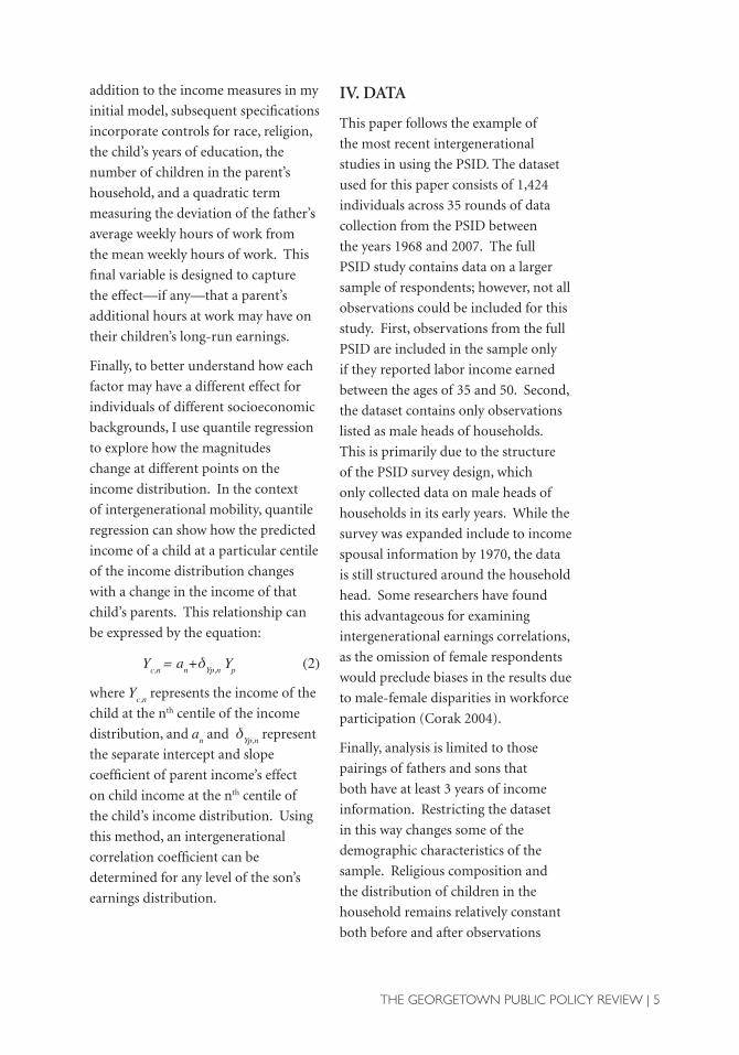
be expressed by the equation:

Yc,n = an+δYp,n Yp (2)

where Yc,n represents the income of the

child at the nth centile of the income

distribution, and an and δδYp,n represent

the separate intercept and slope

coefficient of parent income’s effect

on child income at the nth centile of

the child’s income distribution. Using

this method, an intergenerational

correlation coefficient can be

determined for any level of the son’s

earnings distribution.

Iv. data

This paper follows the example of

the most recent intergenerational

studies in using the PSID. The dataset

used for this paper consists of 1,424

individuals across 35 rounds of data

collection from the PSID between

the years 1968 and 2007. The full

PSID study contains data on a larger

sample of respondents; however, not all

observations could be included for this

study. First, observations from the full

PSID are included in the sample only

if they reported labor income earned

between the ages of 35 and 50. Second,

the dataset contains only observations

listed as male heads of households.

This is primarily due to the structure

of the PSID survey design, which

only collected data on male heads of

households in its early years. While the

survey was expanded include to income

spousal information by 1970, the data

is still structured around the household

head. Some researchers have found

this advantageous for examining

intergenerational earnings correlations,

as the omission of female respondents

would preclude biases in the results due

to male-female disparities in workforce

participation (Corak 2004).

Finally, analysis is limited to those

pairings of fathers and sons that

both have at least 3 years of income

information. Restricting the dataset

in this way changes some of the

demographic characteristics of the

sample. Religious composition and

the distribution of children in the

household remains relatively constant

both before and after observations

6 | cooper

with missing income data are dropped.

Racial/ethnic composition change

more noticeably, with the proportion

of white respondents growing by

roughly seven percentage points, from

58.22 percent of the full sample to

65.10 percent in the paired father-son

data. This corresponds to a slight drop

in the number of black respondents,

from 33.92 percent down to 31.39

percent of the sample, and a more

pronounced decrease in the number of

Hispanic and Asian respondents, from

3.58 percent down to 1.62 percent,

and 0.90 percent to 0.21 percent,

respectively.

This drop in the proportion of

Hispanic and Asian respondents is

an unfortunate consequence of the

unique data requirements of this type

of study. For the purpose of examining

intergenerational changes and

relative magnitudes of socioeconomic

transmission channels, the sample is

still valuable; however, conclusions

about racial and ethnic differences may

warrant further research with a more

diverse sample.

Table 1 lists the descriptive statistics

for observations used in the

intergenerational model. At an

inflation-adjusted value of $53,190.04

for fathers and $53,495.25 for sons,

the paired observations have higher

income levels than the larger U.S.

population; in 2007, mean income

for males in the U.S. was $47,137.

Indeed, the mean income values for

the paired subsample are noticeably

higher than even for the larger PSID

dataset—$40,788.67 for fathers and

$48,000.36 for sons.1 We can speculate

that wealthier families may have

stronger ties to social and professional

networks that facilitate easier tracking

by the survey’s administrators.

Moreover, the data requirements of

multiple years of income data precludes

ex ante those respondents who have

struggled to maintain employment,

whose mean incomes would likely be

considerably lower than the paired

father-son subsample.

While this deviation from the larger

US population again speaks to the

difficulty of maintaining a truly

representative multi-generational

dataset, the more interesting

observation is that the inflation-

adjusted incomes for fathers and

sons are virtually identical. After

adjusting for inflation, not only is

there no change in mean income

between the generations, the median

income appears to have declined: from

$46,091.44 in the fathers’ generation to

$41,760.90 in the sons’.

Table 2 reports the distribution of the

sons’ mean labor income by the race

of the household head for the paired

father-son observations used in the

intergenerational model. To highlight

particular differences with the larger

PSID dataset, the table includes the

distribution of the sons’ mean income

for the larger set of all sons, ages 35 to

50.

Table 3 shows the distribution of sons’

mean income by religious preference

1A comparison of descriptive statistics for both the paired subsample and the larger PSID dataset can be found in the appendix of Cooper’s full thesis on the Georgetown Public Policy Review website, www.gppreview.com.


Note: Labor Income and Work Hours for each observation are recorded for multiple years, 1968-2007, when the respondent was between the ages of 35 and 50. For this reason, descriptive statistics of each individual year are omitted. 1Average number of children calculated during years when head of household is between ages 35 and 50.

Table 1. Descriptive Statistics – Paired Father & Son Observations

Table 2. Distribution of Sons’ Labor Income by Race

Note: Calculations based upon PSID data for years 1967-2007 for male heads of households reporting at least three years of labor income earned between the ages 35 and 50.

for the paired father-son subsample.

While there was again some bias

toward wealthier respondents in

the paired subsample, the overall

distribution of religious preferences

between the full sample and the paired

father-son subsample is considerably

more consistent than the racial

distribution.

Table 4 shows the distribution of the

number of children in each household

during the father’s prime earning years

and the mean labor income for each

family size; the numbers are fairly

consistent across both the full data set

and the paired sub-sample.

8 | cooper

Table 4. Distribution of Sons’ Labor Income by Number of Children in Father’s Family


Table 3. Distribution of Sons’ Labor Income by Religious Affiliation



v. estIMatIon resuLts

A) OLS Estimation

The OLS results for the basic

intergenerational model are presented

in Table 5. Column 1 describes strictly

the effect of the log of the father’s

average labor income on the log of

the son’s average labor income. The

results indicate a highly significant

intergenerational income elasticity

of 0.417. Without controlling for

any other factors, every one percent

increase in the father’s long-run

income leads to a 0.417 percent

increase in the son’s long-run income,

meaning roughly 40 percent of a child’s

long-run income is predicted by the

income of their parents. This result is

consistent with recent research in this

field (Hertz 2002; Grawe 2004; and

Solon 2009).

Column 2 is the model controlling

for the son’s years of education. Once

again, the results are highly significant

and show a noticeable drop in the

independent effect of father’s income

on son’s income, down to 0.27. Eide

and Showalter (1999) observe a similar

decrease in the independent effect of

the father’s income from 0.34 to 0.24

when controlling for the son’s level of

education.

The model in Column 3 adds an

additional control for the number

of children in the father’s household

(each additional sibling to the sons in

the model). This model indicates a

significant, negative effect, predicting

that for each additional child in the

father’s household we expect a decrease

in the son’s long-run earnings of

1.9 percent. According to Becker’s

hypothesis (1983), this effect is

essentially the diluting of the parents’

human capital resources as they are

divided among a greater number of

children.

Hertz (2002) speculates that the

economic mobility of children may

also be influenced by work habits

they observe in their parents—that

children of homes where parents spend

long hours in the labor market might

exhibit a stronger work ethic and

thus greater economic mobility. He

models this possibility using indicator

variables for household heads who

work 2,000 to 3,000 hours annually

and more than 3,000 hours annually,

yet finds no significant effects. The

model in column 4 tests this same

hypothesis, but contains controls for

the deviation of the father’s average

weekly number of work hours from

the mean number of work hours, and

a quadratic term to allow for a change

in the direction of the effect. When

holding the father’s income constant,

we find that additional hours of work

beyond the weekly mean of forty has a

small, decreasing negative effect upon

the son’s long-run income. Although

the coefficient on the linear component

of this variable is not individually

significant, a joint test of the linear

and quadratic variables does indicate a

significant effect

(F(2, 1357)=3.96, p=0.019). The

magnitude of this effect is so small that

that we cannot draw major conclusions

from these findings; however, the

sign of the effect, and its persistence

10 | cooper

It is also interesting to note that

omitting the labor-hours variable in

Models 1, 2, and 3 places a noticeable

downward bias on the father’s income

coefficient. In the model in column

3, the coefficient on the log of the

father’s income predicts that a one

percent increase in the father’s income

will lead to a 0.255 percent increase

in the son’s income. Yet in column

4, after controlling for the father’s

average weekly work hours, a one

percent increase in the father’s income

now predicts a 0.30 percent increase

in the son’s income. This apparent

bias may speak to the same effect of

additional hours spent at work rather

than at home. Children born to fathers

making more money for the same

across further specifications, suggests

a different interpretation from Hertz’s

initial speculation. The additional

hours beyond the mean that parents

spend in the labor market may not

instill a stronger work ethic in their

children, but, instead, may actually

have negative consequences as each

additional hour of work represents one

fewer hour available for the parent to

engage in the child’s development.2

Table 5. OLS Results of the Intergenerational Model with Controls for Son’s Years of Education, Siblings, and Father’s Weekly Work Hours

Note: *** p < 0.01; ** p< 0.05; *p<0.10. Calculations based upon PSID data for years 1967-2007 for male heads of households reporting at least three years of labor income during the years when they were ages 35 to 50. Standard errors in parentheses.

“The additional hours beyond the mean that parents spend in the labor market may not instill a stronger work ethic in their children, but, instead, may actually have negative consequences.”


hours of work will be better off than

those working additional hours to

earn the same income. These findings

are suggestive, but they are far from

conclusive.

Table 6 shows the OLS results for the

intergenerational model with indicator

variables for both race and reported

religion.

The model with controls for race

shows significant negative effects for

the individual coefficients on the black

and Hispanic indicators. Overall, the

full set of race variables are jointly

highly significant (F(6, 1353)=10.03,

p<0.0001). It is interesting to note

how dramatically the independent

effect of the father’s income variable

decreases after controlling for race. At

0.30 in the basic human capital model

shown in Column 1, the coefficient on

father’s income drops to 0.202 in the

model with racial controls. On one

hand, this drop can be viewed as a good

thing, as it indicates that when race

is held constant, there may be greater

economic mobility than the basic

model suggests. Unfortunately, it also

implies that race is clearly an important

mitigating factor in intergenerational

outcomes.

The large, significant, negative

coefficients on the black and Hispanic

variables, contrasted with the large

positive coefficient on the Asian

variable, underscore this fact. With

a value of 0.544 in the racial model,

or 0.644 in the model controlling

for race and religion in Column 4,

the coefficient on the Asian variable

indicates that Asian sons are predicted

to have a mean income that is between

72 percent and 90 percent larger than

the mean income of white sons.3

Although Asian respondents may have

significantly larger mean incomes,

the magnitude of this difference is

skewed by the small number of Asian

respondents in the paired father-son

subsample with an unrepresentative

mean income.

Still, with these subsample

characteristics in mind, it is particularly

noteworthy that the coefficient on the

Hispanic indicator is significant and

shows a large negative effect. Like the

Asian subsample used in the model, the

Hispanic father-son pairs have a much

larger mean income than the full data

set: $63,349.31 in the paired subsample

versus $38,426.38 in the full data set.

Yet, after controlling for education,

work hours, and the number of

children in the father’s household, the

coefficient on the Hispanic variable

indicates that Hispanic sons have

incomes 22 percent lower than white

sons, holding their father’s income

equal. For black respondents, the

effect is even more pronounced: with

a coefficient of -0.344, black sons

typically have incomes 29 percent

lower than white sons with equivalent

2 See Phillips (2002) for a summary of related literature.

“...there may be greater economic mobility than the basic model suggests. Unfortunately...race is clearly an important mitigating factor in intergenerational outcomes.”

12 | cooper

parental incomes. As noted before, the

proportion of minority respondents

in the sample is small—particularly

for Hispanic and Asian respondents—

making it difficult to investigate why

such racial disparities in economic

mobility exist. Nevertheless, these

results reinforce previous findings that

such disparities do exist and are worthy

of further investigation with more

representative data sets.

Theoretically, religion may play a

similar role in the transmission of

economic status. As Bowles and Gintis

(2002) explain, “economic success

is influenced not only by a person’s

traits, but also by characteristics of the

group of individuals with whom the

person typically interacts.” Religious

affiliation can influence economic

mobility through the provision of

social and job networks, but also in

more nuanced ways, such as increasing

conformity to particular social norms

and practices that may or may not

be consistent with greater economic

success (Borjas 1995; Durlauf

2001). After controlling for race, the

coefficients on the Baptist, Protestant,

Catholic, and Jewish indicator variables

all showed a significant, positive effect

upon the log of son’s income. The

largest of these effects is for Jewish

sons, who are predicted to earn 25.7

percent more than atheist or agnostic

sons with fathers of equivalent income.

Similarly, Catholic sons earn 20.6

percent more than atheist or agnostic

sons, while Protestant and Baptist sons

earn 21.5 percent and 9.6 percent more,

respectively.

The fact that these four religious

affiliations have a positive effect could

demonstrate a larger, general positive

effect of religious participation. On

a basic level, religious communities

are incubators of social capital (Smidt

2003). They can provide sources of

additional education for children—

such as Sunday School or Hebrew

classes—and can expand job networks.

Additionally, religious communities

often provide the type of extended

social safety net that can safeguard

members against crises and income

shocks that may endanger children’s

long-run economic potential (Cnaan

1999).

B) Quantile Estimation

Regression techniques that estimate

effects at specific points on the income

distribution can be more useful

in exploring how social mobility

changes at different positions on the

socioeconomic ladder.

Table 7 reports the OLS and quantile

regression estimations of the

intergenerational income elasticity at

3 The percentage differences are calculated for each regression coefficient using the formula. See Wooldridge (2009), p. 233 for further details.

“The fact that these four religious affiliations have a positive effect could demonstrate a larger, general positive effect of religious participation...religious communities are incubators of social capital...they can provide sources of additional education for children.”


Table 6. OLS Results of Intergenerational Model with Controls for Race and Religion

Note: *** p < 0.01; ** p< 0.05; * p<0.10; Race dummy “white” and religion dummy “Other, Atheist, Agnostic, No religion” omitted as reference group. Calculations based upon PSID data for years 1967-2007 for male heads of households reporting at least three years of labor income during the years when they were ages 35 to 50. Standard errors in parentheses. Only significant coefficient results shown; controls for additional race and religion values not displayed.

14 | cooper

Table 8 reports the OLS and quantile

estimation results for four separate

quantile regressions. The first model is

the baseline intergenerational income

elasticity model previously reported.

Model 2 adds a control for the son’s

years of education. Model 3 adds the

number of children in the father’s

household. Model 4 contains the

quadratic term for the deviation of the

father’s weekly work hours from the

mean. The results are reported in this

fashion to allow comparisons between

the strength of the intergenerational

income elasticity in Model 1 and its

effects in subsequent models across

the conditional distribution of the

son’s income. As with the OLS results,

changes in the magnitude of the

coefficient on father’s income, after

controlling for additional factors,

reflect the relative importance of each

of these factors in the transmission of

economic status.

the 5th, 10th, 25th, 50th, 75th, 90th,

and 95th percentiles of the income

distribution in the son’s generation.4

All of the estimates are statistically

different from zero at the 1 percent

level. The results clearly show a

decreasing trend in the effect of the

father’s income as the son’s income

level increases, with a coefficient on the

father’s log income of 0.63 at the 0.05

quantile, declining all the way to 0.25 at

the 0.95 quantile.

These results are consistent with

previous estimations that found a

declining trend in the intergenerational

income elasticity from 0.77 for the

0.05 quantile down to 0.19 at the 0.90

quantile (Eide and Showalter 1999;

Grawe 2004). These findings reinforce

the hypothesis that the persistence

of economic status is stronger for

those at the bottom of the income

distribution than for those at the top.

Put differently, it suggests that each

additional dollar for a poor father has

a stronger positive effect upon the

long-run income of his child than each

additional dollar’s effect on the long-

run income of a rich father’s son.

Table 7. Quantile Regression Results of Baseline Intergenerational Model

Note: *** p < 0.01; ** p< 0.05; * p<0.10; Race dummy “white” and religion dummy “Other, Atheist, Agnostic, No religion” omitted as reference group. Calculations based upon PSID data for years 1967-2007 for male heads of households reporting at least three years of labor income during the years when they were ages 35 to 50. Standard errors in parentheses. Only significant coefficient results shown; controls for additional race and religion values not displayed.

Dependent Variable: Log of Son’s Income

4 Because the quantile regression models used throughout this paper are all estimated on the conditional distribution of son’s income, the terms “percentile” and “quantile” are used interchangeably to refer to the different levels of son’s income.


becomes relatively more valuable at

the tails of the distribution and most

valuable at the top. It is possible that

changes in the income distribution

from the time of their study—their

paper employs PSID data of the father’s

generation in the years 1968-1970 and

the son’s generation in years 1984-

1991—may account for this change.

An increasing concentration of US

wealth in the upper percentiles—

consistent with this paper’s previously

noted increased income inequality —

combined with unequal wage growth

over the last two decades, may be

driving this difference in results.

The basic interpretation that education

has become more valuable at the top

of the income distribution than at the

median is potentially unsettling; such

differences can only serve to further

stratify the distribution of income.

For a useful comparison, similar to

Eide and Showalter’s (1999) paper,

consider the differences in log earnings

for individuals at the 90th and 50th

percentiles of income for those who

have completed college versus those

who have only completed high school.

Looking first at Model 2, we once again

see a highly significant, declining effect

of father’s income as the son’s income

level increases. The magnitude of this

effect after controlling for education,

however, changes dramatically at all

income levels. At the 5th percentile,

the coefficient on the father’s income

drops from 0.633 in Model 1 to 0.363

in Model 2, a nearly 43 percent change.

The drop at the 90th percentile is even

more pronounced, falling from 0.384

in Model 1 to 0.180 in Model 2, a 53

percent change. All other quantile

estimates of the father’s income

coefficient are reduced in Model 2 by

roughly a third. This is consistent with

the reduction that occurs in the OLS

model, a 34.8 percent drop, as well as

with previous research (see Eide and

Showalter 1999).

Interestingly, the magnitude of son’s

level of education appears to have a

somewhat parabolic shape across the

distribution, going from 0.155 and

0.157 respectively at the 5th and 10th

percentiles, down to a low of 0.124 at

the 50th percentile, then back up to

highs of 0.159 and 0.182 at the 90th

and 95th percentiles. This effect is

significantly different from zero at the

1 percent level in all cases.5 This result

is noticeably different from Eide and

Showalter’s (1999) observation that the

son’s years of schooling have the largest

effect at the 10th percentile, and the

smallest at the 75th percentile.

Whereas Eide and Showalter could

interpret their results as evidence

that education is more valuable at the

bottom of the income distribution, the

findings above suggest that education

“...we once again see a highly significant, declining effect of father’s income as the son’s income level increases. The magnitude of this effect after controlling for education, however, changes dramatically at all income levels.”

5 This difference in magnitude was significant between the 90th and the 25th, 50th, and 75th percentiles, as well as between the 95th and the 25th, 50th, and 75th percentiles.

16 | cooper

the financial burden of an additional

child may be negligible. For children

who are born into less affluent families

and who still achieve high levels of

income, the impact of additional

siblings on the amount of resources

available to each child is simply not

a significant factor in their eventual

economic success.

For sons born into poverty who

ultimately remain at the lower levels of

the income distribution, the additional

tax credits and income support

measures that are granted for each

additional child in low-income families

may offset some of the decrease in

resources available to each child.

Another possible explanation is that

sons at the lower levels of the income

distribution may lack suitable access

to higher education, i.e., the cost of

post-secondary education may have

been prohibitive for them from the

start. If this is the case, then the added

challenge to that child’s parents of

meeting those costs when an additional

child is born is never a significant

factor. At the 50th and 75th percentile

of the sons’ income distribution,

however, the cost of each additional

child in the father’s household may

have a more substantive impact.

Particularly in the context of education

costs, the possibility of private

schooling or college for a child may

be significantly diminished with an

increasing number of siblings.

Model 4 includes the linear and

quadratic controls for the deviation of

the father’s weekly work hours from the

mean. The quantile coefficients add

some interesting nuance to the OLS

The 50th percentile of log earnings

for college graduates is 11.17, and for

high school graduates it is 10.46—a

difference of 0.65 points. At the 90th

percentile, the log of earnings for

college graduates is 11.94, while for

high school graduates it is 11.17—a

difference of 0.77 points. This simple

comparison highlights the effect

described in the quantile results: the

four years of college for sons at the top

of the income distribution correlates

with a larger increase in income than it

does for sons at the median income. If

this trend continues, it will only further

expand the already broadening gap in

distribution of income in the US.

Model 3 controls for the number of

children in the father’s household to

capture the effect of each additional

sibling on the observed son’s long-run

earnings. In the quantile estimation,

the coefficient on this variable is

significant only at the 50th and 75th

percentile of sons’ income, although,

at all levels of income, the effect is

negative and of roughly the same

magnitude. The addition of this

variable into the model does reduce

the magnitude of the father’s income

coefficient in all but the 5th percentile,

but only by a small percentage. For

children born into wealthier families,

“The basic interpretation that education has become more valuable at the top of the income distribution than at the median is potentially unsettling; such differences can only serve to further stratify the distribution of income.”

Note: *** p < 0.01; ** p< 0.05; * p < 0.10. Results calculated using quantile estimation based upon PSID data for years 1967-2007 for male heads of households reporting at least three years of labor income during the years when they were ages 35-50. Standard errors generated using bootstrapping with 100 repetitions.

Table 8. Quantile Regression Results of Intergenerational Models with Controls for Son’s Education Level, Number of Children in Father’s Household, and Deviation of Father’s Weekly Work Hours

17

18 | cooper

earns the same level of income for less

work is coming from a more privileged

starting position.

The other important result to note

from Model 4 is the change in strength

of the father’s income coefficient. In

the 50th through 95th quantiles, the

addition of the work hours variable

causes the coefficient on the log of

fathers’ income to rise dramatically,

in some cases more than doubling

in magnitude. For example, the

coefficient on the father’s income

variable in Model 3 at the 90th quantile

is 0.169. After controlling for the

father’s weekly work hours in Model

4, this coefficient rises to 0.344, an

increase of 104 percent. Only at the

5th, 10th and 25th percentiles does

the coefficient on the father’s income

variable decrease with the addition

of the father’s work hours variable.

Given that the other variables in the

model—son’s years of education

and the number of children in the

father’s household—remain relatively

unchanged, this suggests two possible

conclusions: 1) For sons at the bottom

of the income distribution, there

are other omitted factors that are

still more important in explaining

these individuals’ eventual economic

position; and 2) for children at the

top of the income distribution, their

parents’ level of income is a particularly

important factor, especially when

the parents’ hours of work are held

constant.

Finally, Table 9 presents the quantile

estimation results for the regression

predicting son’s log income, with

controls for father’s log income, the

results. Although the linear term in

the OLS regression is not significant at

standard levels, the quantile estimation

reports highly significant effects for

both the linear and quadratic terms at

the 75th and 90th percentiles. Both

terms are jointly significant at the 50th

and 95th percentiles. In these cases,

the results show a small, decreasing

negative effect of roughly -0.01, which

can be interpreted as a reduction of

roughly 1 percent in the son’s income

resulting from each additional hour his

father spends at work each week.

As noted in the OLS results, this

negative coefficient implies that, all else

being equal, sons whose fathers spend

additional hours in the workplace

are predicted to achieve lower long-

term earnings than their peers whose

fathers earned the same income with

fewer hours of work. According to the

quantile estimation, this effect applies

particularly to sons at higher levels of

the income distribution, which may

be more demonstrative of selection

issues than a causal relationship. Sons

who achieve high levels of income, yet

whose fathers worked longer hours

than their peers, may have simply

come from less affluent backgrounds.

In other words, the son whose father

“For children who are born into less affluent families and who still achieve high levels of income, the impact of additional siblings on the amount of resources available to each child is simply not a significant factor in their eventual economic success.”


the theory that religious communities

may provide some level of social

insurance for families at the lower end

of the income distribution that might

otherwise fall into deeper levels of

poverty.

vI. concLusIon

The results presented in this paper

confirm what an increasing number

of researchers have concluded:

socioeconomic mobility in the US is

significantly lower than was previously

thought and individuals’ long-run

economic position remains closely tied

to the economic status into which they

are born. Avoiding the use of a specific

set of calendar years, and comparing

the individual earnings of both fathers

and sons at equivalent points in the

lifecycle, I find an intergenerational

correlation of income consistent with

previous findings that, on average,

roughly 40 percent of a son’s income

can be predicted by the income of his

father. More importantly, I find that

the intergenerational correlation of

earnings is considerably stronger at

lower levels of the income distribution,

just as earlier research has also

concluded. This phenomenon is only

likely to grow stronger as income

inequality in the US continues to

expand.

son’s years of education, the number

of children in the father’s household,

the father’s weekly work hours and

indicator dummies for race and

religious preference. Only variables

with significant results are shown.

After controlling for race and religion,

we again see similar trends in the

magnitude of the father’s income as

observed in Model 4, with a high value

of 0.257 at the 95th percentile and

a low of 0.08 at the 10th percentile,

although this value is not statistically

significant. The effects for son’s years of

education, the number of children in

the father’s household, and the father’s

weekly work hours remain relatively

unchanged.

Of the racial indicators, the coefficient

on the black variable remains negative

and highly significant at all levels of

income, although it does diminish in

strength through the middle of the

distribution when compared to the

tails. The coefficient has its strongest

negative value of -0.4 at the 5th

percentile and its weakest negative

effect of -0.25 at the 50th percentile.

This may reflect a growing black

presence in the American middle class,

although black Americans are clearly

still disadvantaged at the highest and

lowest levels of income. As noted in

the OLS results section, the significant,

large positive effects shown for Asians

are likely driven by a lack of adequate

Asian participants in the sample.

The positive effect of religious

participation observed in the OLS

estimation remains significant only

at the lower end of the son’s income

distribution. This is consistent with

“...socioeconomic mobility in the US is significantly lower than was previously thought and individuals’ long-run economic position remains closely tied to the economic status into which they are born.”

20 | cooper

Table 9. Quantile Estimation of the Log of Son’s Income by Father’s Income, Son’s Education, Number of Siblings, Father’s Weekly Work Hours, Race, and Religion

Note: *** p < 0.01; ** p< 0.05; * p < 0.10. Results calculated using quantile estimation based upon PSID data for years 1967-2007 for male heads of households reporting at least three years of labor income during the years when they were ages 35-50. Standard errors generated using bootstrapping with 100 repetitions.


representative data set, this approach

may not provide major insight into

why race has such a strong effect upon

economic mobility.

Although previous research has

noted religion’s possible role in the

transmission of economic status, the

results presented here add some nuance

to this relationship. In cases where

religious affiliation has a significant

effect upon long-run incomes, this

effect is largely limited to individuals at

lower levels of the income distribution.

This could indicate the role of some

religious communities as providers of

an extended social safety net outside

the traditional family structure. Far

from being conclusive, this finding

could also be an interesting focus for

future research.

Finally, my analysis of how fathers’

average time spent at work might

affect sons’ long-run income shows

a potentially interesting effect. It

is not a shocking idea that fathers

who have to work extra hours to

achieve a comparable level of income

may be losing hours to spend on

their children’s development. Yet,

as many Americans struggle to

identify a suitable balance of time

spent in labor versus leisure, the idea

that additional time spent at work

may have a statistically observable,

detrimental effect upon children’s

long-run outcomes would have

important implications for parents and

policymakers. Still, the effect observed

in this study is too small and not

robust enough across different model

specifications to arrive at any definitive

conclusions.

As one would expect, education

continues to have a strong, positive

effect on children’s long-run economic

prospects. However, in contrast to

previous research, I find that the

effect of education may be shifting

to benefit those at the top of the

income distribution more than

those at the bottom or in the middle

class. Given the aforementioned

trends in income inequality, this

finding has particularly disturbing

implications. If an additional year

of education has a stronger positive

effect for a child at the top of the

income distribution than one at the

median, then this can only further

widen the income gap. Furthermore,

if this result is a consequence of

differences in the quality of education

available to different income classes,

the phenomenon will only reinforce

itself. Without conscious policies to

make high-quality education available

to all income groups, education will

not serve to level the playing field,

but rather will exacerbate existing

differences in economic mobility such

that the rich and the poor will be

“playing” on two completely separate

fields.

Attempts to identify how racial factors

might contribute to economic mobility

are less conclusive, although they show

that black children in America continue

to be at a disadvantage to their white

counterparts, even when their father’s

incomes are equivalent. Similar trends

may exist for Hispanic children as well.

Unfortunately, the models employing

racial indicators are limited by a lack

of suitable data, and even with a more

Ultimately, these findings cannot

serve as a prescription for individual

economic success; perhaps the

American dream cannot be unlocked

so much as it can be promoted. In this

spirit, the findings of this research can

be used to inform policy formation

and prioritization so that it better

promotes equality of economic

opportunity. Policies that strengthen

education for the lower and middle

classes, that seek to reduce racial

disparities, that recognize the role of

religious participation and family size

on economic outcomes, and that are

cognizant of parents’ time spent in the

workplace can all serve to manifest

greater intergenerational mobility.

22 | cooper

“...perhaps the American dream cannot be unlocked so much as it can be promoted...Policies that strengthen education for the lower and middle classes, that seek to reduce racial disparities, that recognize the role of religious participation and family size on economic outcomes, and that are cognizant of parents’ time spent in the workplace can all serve to manifest greater intergenerational mobility.”


Grawe, Nathan D. “Intergenerational mobility for whom?” in Generational income mobility in North America and Europe, edited by Miles Corak (Cambridge: Cambridge University Press), 2004, 58-89.

Hertz, Tom. “Understanding Mobility in America.” Center for American Progress (2006). http://www.americanprogress.org/issues/2006/04/Hertz_MobilityAnalysis.pdf.

Institute for Social Research.“An Overview of the Panel Study of Income Dynamics,” University of Michigan, [Website] http://psidonline.isr.umich.edu/.

Koenker, Roger, and Gilbert Bassett. “Robust Tests for Heteroscedasticity Based on Regression Quantiles.” Econometrica 50, no. 1 (January 1, 1982): 43-61.

Lee, Chul-In, and Gary Solon. “Trends in Intergenerational Income Mobility.” Review of Economics and Statistics 91, no. 4 (November 1, 2009): 766-772.

Phillips, Katherin Ross. “Parent Work and Child Well-Being in Low-Income Families.” Text, June 25, 2002. http://www.urban.org/publications/310509.html.

Roemer, J. E. “Equal opportunity and intergenerational mobility: going beyond intergenerational income transition matrices.” in Generational income mobility in North America and Europe, edited by Miles Corak (Cambridge: Cambridge University Press), 2004: 48–57.

Sewell, William H. and Hauser, Robert M. Education, Occupation, and Earnings: Achievement in the Early Career, New York: Academic Press, 1975.

Smidt, Corwin E. Religion as social capital: producing the common good. Baylor University Press, 2003.

Solon, Gary. “Intergenerational Income Mobility in the United States.” The American Economic Review 82, no. 3 (June 1992): 393-408.

Wooldridge, Jeffrey M. Introductory Econometrics: A Modern Approach, (Mason, OH: South-Western Cengage Learning), 2009.

vII. reFerences

Becker, Gary S. Human Capital and the Personal Distribution of Income: An Analytical Approach. Woytinski Lecture No. 1. Ann Arbor: University of Michigan: Institute of Public Administration, 1967.

Becker, Gary S., and Nigel Tomes. “Human Capital and the Rise and Fall of Families.” Journal of Labor Economics 4, no. 3 (July 1986): S1-S39.

Behrman, Jere, and Paul Taubman. “Intergenerational Earnings Mobility in the United States: Some Estimates and a Test of Becker’s Intergenerational Endowments Model.” The Review of Economics and Statistics 67, no. 1 (February 1985): 144-151.

Borjas, G. J. “Ethnicity, Neighborhoods, and Human-Capital Externalities.” The American Economic Review 85, no. 3 (1995): 365–390.

Bowles, Samuel, and Herbert Gintis. “The Inheritance of Inequality.” Journal of Economic Perspectives 16, no. 3 (9, 2002): 3-30.

Cnaan, R. A, and G. I. Yancey. “Our Hidden Safety Net.” Brookings Review 17, no. 2 (1999): 50–53.

Corak, Miles, ed. “Generational Income Mobility in North America and Europe.” Cambridge, England: Cambridge University Press, 2004.

Durlauf, Steven N. “A Theory of Persistent Income Inequality.” Journal of Economic Growth 1, no. 1 (3, 1996): 75-93.

Eide, Eric R., and Mark H. Showalter. “Factors Affecting the Transmission of Earnings across Generations: A Quantile Regression Approach.” The Journal of Human Resources 34, no. 2 (Spring 1999): 253-267.

Fitzgerald, John, Gottschalk, Peter, and Moffitt, Robert. “A Study of Sample Attrition in the Michigan Panel Study of Income Dynamics,” February 1994; revised, October 1996.

Goldin, Claudia Dale., and Lawrence F. Katz. “Long-Run Changes in the Wage Structure: Narrowing, Widening, Polarizing.” Brookings Papers on Economic Activity 2007, no. 2 (2008): 135-165.

24 | cooper


armed conflict and early childhood outcomes in ethiopia and perú

By Kate Anderson Simons

experts unanimously agree that armed conflict is harmful to children. However, few studies exist that examine the link between armed conflict and language and cognitive

development in the early years. this paper uses the young lives data from perú and ethiopia to analyze the relationship between armed conflict and child outcomes in early language and cognitive development, using two standardized measures, the peabody picture vocabulary test (ppvt) and the cognitive Development Assessment-Quantitative (cDA-Q), both administered at or near age five. The results show that, after holding a variety of child, family, and community factors constant, living in a region of the country that has experienced war more recently is associated with lower receptive language (PPVT) scores in Perú, while intensity of the conflict is associated with lower ppvt scores in ethiopia. preschool attendance and family wealth are strong predictors of higher PPVT scores. These findings suggest that children living in conflict or post-conflict situations are particularly vulnerable to language disadvantages that could impact opportunities throughout life. therefore, early childhood development should be prioritized in conflict-affected areas, with a special emphasis on high-risk populations to ensure that coming generations of rural and poor children are given opportunities to thrive.

Kate Anderson Simons

completed the Master of Public Policy

at the Georgetown Public Policy

Institute in 2011. Adam Thomas, Ph.D.,

served as her thesis adviser. Currently,

Kate is a Monitoring & Evaluation

Consultant at the Brookings Institution,

Center for Universal Education, where

she is working to develop a system

of internationally comparable learning

metrics.

26 | SiMonS

I. IntroductIon

An estimated one billion children

under the age of eighteen live in a

country affected by armed conflict,

and approximately 300 million

children younger than age five live

in conflict-affected areas (UNICEF

2009a). The consequences of armed

conflict are widespread. Children can

experience war firsthand through

witnessing violence, being injured or

killed in combat, or being recruited as

a child soldier. If a child is fortunate

enough to live in an area outside the

immediate vicinity of the conflict, a

family member such as a parent or

older sibling may leave to fight in

the war. This can potentially cause a

decrease in family income, loss of a

family member, or an increase in family

stress. Even if the child’s family remains

intact during the conflict, the state will

likely use all available resources to fight

the war and cut back on education,

social, and health services. These

factors lead to what Marshall & Gurr

(2005) call the “conflict-poverty trap,”

whereby political instability leads to a

breakdown of state-provided services,

which in turn leads to increasing

poverty and further instability.

The United Nations Children’s Fund

(UNICEF) acknowledges, “The

impact of armed conflict on children

remains difficult to fully ascertain. The

information available is patchy, and it

varies in both specificity and accuracy”

(UNICEF 2009a 18). Children are

renowned for being resilient to negative

events early in life, but how far does

this resiliency extend? Using data from

the Young Lives Project, this paper

will address the following question:

Do children living in conflict-affected

areas exhibit lower levels of language

and cognitive development? While

war is undoubtedly damaging to all

children and adolescents, it is possible

that the youngest children experience

the most irreversible consequences

of these atrocities. How are the

youngest children faring in wartime

and in the wake of armed conflict?

This question has important policy

implications for humanitarian relief

and continuity of social protection

during conflict. If these negative early

experiences do indeed impact child

cognitive development, donors and

humanitarian relief programs should

focus on strategies to ameliorate this

damage.

II. conceptuaL ModeL and hypothesIs

Low levels of early language and

cognitive ability can have lifelong

consequences (Currie & Thomas 1999;

Hanushek & Woesmann 2009). Child

development is a complex, dynamic

process determined by a variety of

genetic and environmental factors,

with the first five years of life being

“Do children living in conflict-affected areas exhibit lower levels of language and cognitive development? While war is undoubtedly damaging to all children and adolescents, it is possible that the youngest children experience the most irreversible consequences of these atrocities.”


critical to later development. When a

child lives under conditions of extreme

adversity, the short-term physiological

and psychological adjustments that

allow him or her to survive can cause

a range of health and developmental

problems later on (Thompson 2001).

Armed conflict also brings a host of

negative externalities for the citizens of

a country (UNICEF 2009a; UNESCO

2011). Figure 1 shows the conceptual

relationship between armed conflict

and child cognitive outcomes.

Given this conceptual relationship,

I hypothesize that living in regions

where there has been recent conflict

has a significant negative impact

on child language and cognitive

development. Therefore, I predict that

the more recently an armed conflict

occurred in a region, the lower said

children will perform on language and

cognitive development assessments,

holding child, family, and community

factors constant. I also predict that the

intensity of a conflict is associated with

language and cognitive development,

with children who live in regions with

more intense conflicts scoring lower

on measures of language and cognitive

ability.

III. Background

Large-scale data on language and

cognitive development is limited

in developing countries, especially

countries affected by conflict.

Therefore, to examine the relationship

between conflict and cognitive

development, it was necessary to

find high-quality research studies on

children in countries where conflict

occurred recently. The Young Lives data

set—a longitudinal study of children in

poverty—offers comprehensive child-

and family-level data from Ethiopia,

Figure 1: Conceptual Model

28 | SiMonS

India (Andhra Pradesh), Perú, and

Vietnam. Two of these countries,

Ethiopia and Peru, experienced armed

conflict during the past fifteen years.1

The conflict in these two countries

varied by region, with active conflict

occurring in some regions but not

in others. This allows for analysis

of the relationship between child

development and conflict within each

country. General statistics on Ethiopia

and Perú, including data on recent

conflicts, are described below.

Ethiopia

In Ethiopia, children and families

face multiple challenges in early

childhood and beyond. Children in

Ethiopia consistently score low on a

range of developmental indicators and

child outcomes (World Bank 2010;

UNESCO 2010). In 2005, 78 percent

of Ethiopians lived on less than $2

USD per day and 39 percent lived on

less than the international poverty line

of $1.25 USD per day (World Bank

2010). The under-five mortality rate

is 109 per 1,000 births2 and 20 percent

of Ethiopian infants are born with

low birth weights (UNICEF 2009b).3

Educational attainment in Ethiopia is

among the lowest in the world. Only

36 percent of adults and 50 percent of

youth are literate (UNESCO 2010).4

Two significant armed conflicts

occurred between 1980 and 2007

in the regions where the Ethiopian

study children lived. The largest was a

border dispute between Ethiopia and

neighboring Eritrea (Uppsala Conflict

Data Program 2011; Beenher 2005). In

1998, Eritrean troops entered an area

under Ethiopian control. Because of

deteriorating relations between the two

countries, the event triggered an all

out war that lasted from 1998 to 2000.

A peace accord was signed in 2000;

however, the two countries have failed

to agree on the demarcation of the

border. Between 70,000 and 100,000

lives were lost in this conflict (ICG

2003; Marshall 2010).

Another recent conflict in Ethiopia is

the Oromo independence movement.

Oromia is the largest region in

Ethiopia, and the Oromo ethnic group

makes up around half of the Ethiopian

1 While India has engaged in armed conflict during the past 15 years, notably against Pakistan over the disputed Kashmir region, the Young Lives data focuses on the State of Andhra Pradesh, which has experienced no significant armed conflict since 1947. Source: Uppsala Conflict Database, 2010.

2 By comparison, the under-5 mortality rate is 6 deaths per 1,000 births in industrialized countries and 65 deaths per 1,000 births across all countries.

3 This figure can be compared with the world average of 16 percent.

4 By contrast, the average literacy rates in developing countries are 80 percent (adult) and 87 percent (youth).

“The under-five mortality rate is 109 per 1,000 births and 20 percent of Ethiopian infants are born with low birth weights. Educational attainment in Ethiopia is among the lowest in the world. Only 36 percent of adults and 50 percent of youth are literate.”


population. Led by the Oromo

Liberation Front (OLF), the conflict

has been ongoing since the rebel

group launched an armed struggle for

independence in 1973. An estimated

2,000 lives have been lost in this

conflict (Marshall 2010).

Perú

In Perú, children fare better than

children in Ethiopia. In 2007, 18

percent of citizens lived on less than $2

USD per day and only 8 percent lived

on less than $1.25 USD per day (World

Bank 2010). The under-five mortality

rate in Perú is 24 per 1,000 births

and 8 percent of Peruvian infants are

born with low birth weights (UNICEF

2009b). Perú has very high literacy

rates—90 percent of adults and 97

percent of youth are literate (UNESCO

2010).

In Perú, intrastate conflict has been

ongoing since 1965 (Uppsala Conflict

Data Program 2011). Two Marxist

revolutionary groups, the Sendero

Luminoso (or “Shining Path”) and the

Movimiento Revolucionario Túpac

Amaru (MRTA) emerged in the early

1980s, engaging in a violent insurgency

that was accompanied by human rights

abuses on all sides. From 2000 to 2006

the conflict was dormant, but in 2007

the Sendero Luminoso movement

became active again and the struggle

continues today. A conservative

estimate of lives lost is 30,000, with

many civilian casualties (Marshall

2010).

The other recent conflict affecting

citizens in Perú was the Perú-Ecuador

border dispute of 1995. This dispute

primarily occurred in the Amazonas

region. Approximately 1,000 battle

related deaths occurred during this

conflict (Uppsala Conflict Data

Program 2011; Marshall 2010).

Iv. data and Methods

Data Source

This paper uses child and family-

level data from Young Lives: An

International Study of Child Poverty.

Young Lives is funded by the UK

Department for International

Development (DFID). In this analysis,

I focus on the younger cohort of this

data set. For this cohort, a household

survey was conducted when the

children were approximately one year

old (in 2002) and again when the

children were between four and six

years old (in 2006-7). Attrition was

very low for this cohort: only slightly

more than 4 percent in both Perú and

Ethiopia dropped out of the study

between the two surveys.

The dataset includes standardized

child assessment measures, as well

as demographic, economic, and

community-level data. Households

were selected randomly within each

sentinel site—a village or community

chosen for having high numbers

“The under-five mortality rate in Perú is 24 per 1,000 births and 8 percent of Peruvian infants are born with low birth weights. Perú has very high literacy rates—90 percent of adults and 97 percent of youth are literate.”

30 | SiMonS

of children living in poverty. The

study designers chose sentinel sites

to construct a dataset that reflected

the regional, cultural, and linguistic

makeup of each country.

Measures

Dependent Variable

The dependent variables for this

analysis are child language and

cognitive scores. Child language

was measured by the Peabody

Picture Vocabulary Test (PPVT), a

standardized assessment of receptive

language. The third edition of the

PPVT (PPVT-III) was used in Ethiopia.

The Spanish version of the PPVT-R,

the Test de Vocabulario en Imagenes

Peabody (TVIP), was used in Perú.

The tests were then translated into

each country’s main languages by

the local team and verified by a local

expert before the pilot study conducted

prior to the second round of data

collection (Cueto, Leon, Guerrero, &

Muñoz 2009). Raw scores are used

instead of standardized scores for the

PPVT because the measure was not

normalized in the countries examined

in this study. Cognitive ability was

measured by the quantitative subscale

of the Child Development Assessment

(CDA-Q).

All observations conducted

under inadequate conditions—

assessments with interruptions, lack

of flat workspace, or a distracting

environment—were dropped from the

analysis. A total of 262 observations

were dropped from the Ethiopia dataset

and 146 observations were dropped

from the Perú dataset. In Perú, dropped

observations were evenly distributed

among the fourteen regions in the

study. However, in Ethiopia, assessment

conditions in the Oromia region were

more frequently reported as inadequate

than those from the other regions in

the study. The implications of this are

discussed in the findings section of this

paper.

Independent Variables

Time since conflict: The year of the

last armed conflict in the region

was determined through a search

of multiple conflict databases and

reviewed by several regional conflict

experts for accuracy. The number of

years between the time the Young Lives

survey was administered and the last

armed conflict were calculated for each

child. The variable includes armed

conflicts that took place any time

between 1980 and 2007.

6 The PPVT-III contains 204 possible items and the TVIP contains 125 possible items.

7 Data on the last conflict were collected from the Uppsala conflict database, Center on Sustainable Peace, Global Security, and the Truth and Reconciliation Commission of Perú reports, and validated by experts in the field of global security.

8 Regions with no armed conflict during this period were coded as having a last conflict in 1980. The year 1980 was chosen as a floor for this variable to ensure that the period of analysis at least covers the adult lives of the parents of the study children. In the regions with no conflict since 1980, further research identified that no significant conflicts had occurred since 1947. The year 2007 is the ceiling because it the last year in which data were collected for this cohort.

9 The highest magnitude of conflict recorded on this scale, which includes all conflicts since 1946, is a level 7. The Ethiopian-Eritrean ethnic conflict that occurred from 1974-1991 and concluded with Eritrean independence was rated a level 6.


Figure 2. Regional Map of Ethiopia Depicting Conflict Intensity

Note: For more information on conflict statistics by region see http://www.younglives.org.uk/our-publications/student-papers/no-time-to-thrive. To view this map in color, see Simons’ full thesis at www.gppreview.com.

Recent conflict: Time since conflict is

also measured by a binary variable for

recent conflict, coded as 1 if there was

conflict since 1995 and 0 if there was

no conflict since 1995.

Intensity of last conflict moderate/

high: I also considered the intensity

of the most recent conflict. For this I

consulted Marshall’s “Major Episodes

of Political Violence” —a list that

assigns magnitudes to conflicts on

a 1-10 scale based on the societal

effects of the conflict (2010). Conflicts

associated with the regions in this study

ranged from a level 1 (just over the

threshold of 1,000 battle-related deaths

to qualify for Marshall’s list) to a level 5

(the Ethiopia-Eritrea border dispute in

1998-2000). The magnitude represents

the impact on the country as a whole;

therefore, while each region likely

experienced the conflict differently,

all regions involved in the conflict are

coded at the same level. Among the

regions in my sample, all conflicts were

coded at a level of 1, 3, or 5. A conflict

was considered to be moderate/high if

it was a level 3 or above. Regions with

no conflict were coded as 0.

Battle-related deaths, total in last

conflict (000s): The number of battle-

related deaths is another proxy for

conflict intensity. Data on battle-related

deaths was not accessible by region,

so the number of deaths for the entire

conflict is used. Data collection for

Round 2 was completed in 2007, so I

did not consider conflicts occurring

after that period.

Figures 2 and 3 show the intensity

of conflict across regions in Ethiopia

and Perú for the regions used in this

analysis.

32 | SiMonS

Figure 3. Regional Map of Perú Depicting Conflict Intensity

Note: These figures were collected from reputable databases on global conflict and security. However, there are conflicting reports for regional-level data on years since conflict and battle-related deaths. The binary variables recent conflict and intensity of last conflict moderate/high attempt to capture the conflict variables using more widely accepted assumptions. To view this map in color, see Simons’ full thesis at www.gppreview.com.

last in conflict, and by a binary variable

expressing whether or not there has

been conflict in the region since 1995.

The second independent variable

of interest is the intensity of the last

conflict, measured by number of battle-

related deaths and magnitude rating.

The theoretical model for this analysis

uses OLS regression as follows:

childoutcomes = β0 + β1(lastconflict) + β2(conflictintensity) + β3x3 + β4x4 + β5x5 + ε

where “childoutcomes” is child

cognitive outcomes, “lastconflict” is

a variable measuring the time since

the region was last engaged in armed

conflict, “conflictintensity” is a variable

The model includes control variables

for child age, gender, stunting, weight-

for-age, preschool attendance, first

language, mother’s education, family

wealth, and rural residence.

Methods

To understand the relationship

between armed conflict and child

development, I use an Ordinary Least

Squares (OLS) regression model. The

dependent variable is child cognitive

outcomes, measured by raw scores on

the PPVT and CDA assessments. The

first independent variable of interest is

time since the last conflict—measured

both by the number of years since the

region where each child lived in was


(s.d.=8.53) in Perú. This means that

on average, children in Ethiopia

could correctly identify 22 pictures of

progressively more difficult vocabulary

words and children in Perú could

identify on average 30 pictures. By

comparison, the mean PPVT raw

score for children of similar ages

exiting Head Start (a federally-funded

preschool program for low-income

children in the United States) is

approximately 57 (U.S. Department of

Health and Human Services 1998).10

measuring conflict intensity, x3 is a

vector of child characteristics, x4 is

vector of family characteristics, and x5

represents community characteristics.

v. resuLts

Descriptive Statistics

This section describes the descriptive

statistics for the dependent and

independent variables for Ethiopia

and Perú. Table 1 shows the complete

descriptive statistics for the sample.

Child Outcomes

The mean PPVT raw score was 21.98

(s.d.=12.56) in Ethiopia and 30.07

Table 1: Descriptive Statistics

10 The mean standard score for 5-year-olds exiting Head Start in 1998 was 93. This corresponds to a raw score of approximately 57.

34 | SiMonS

The mean CDA-Q score for all children

was 8.41 (s.d.=2.52) in Ethiopia and

8.83 (s.d=2.03) in Perú out of 15 total

test items. This means that on average,

children correctly answered between 8

and 9 questions about quantity (more/

less, long/short, etc.).

Conflict Indicators

In Ethiopia, the average number of

years since conflict occurred in each

child’s region was 17.6, with 39 percent

of the study children living in a region

where there has been conflict since

1995. In Perú, the average number

of years since conflict was 8.7 and 79

percent of the children lived in a region

experiencing conflict after 1995.

Regression Results

Using Ordinary Least Squares (OLS),

I estimated three regression models

for each country with PPVT scores

as the dependent variable and three

regression models for each country

with CDA-Q scores as the dependent

variable.

PPVT Results for Ethiopia

Table 2 shows the predicted PPVT

raw scores for children in Ethiopia

and Perú. OLS regression results

for Ethiopia show no significant

relationship between PPVT scores and

time since conflict after controlling

for child, family, and community

characteristics. However, the intensity

of the latest conflict is significantly

negatively associated with PPVT scores.

Model 3 shows that children living in

regions that experienced a moderate

to high-level conflict scored 1.2 points

lower than children who lived in

regions with a low-level conflict or no

recent conflict (p=0.09) . Furthermore,

Model 1 shows that each 1,000 combat-

related deaths were associated with a

0.02 point decrease in PPVT scores

(p=0.07), implying that approximately

50,000 combat related deaths were

associated with a one-point decrease in

PPVT scores.

The assessments obtained under

inadequate conditions were not taken

into account. This was the case in

Ethiopia, where 32 percent of the

observations of the Oromia region

were not included in the analysis.

Omission of these observations may

positively bias the coefficient for

recent conflict. Furthermore, Oromia

is the largest region in the country in

terms of population and area. While

the Oromo Liberation Front conflict

occurred in the Southern and Eastern

areas, it is possible that children and

families in the North and West areas

were not directly affected by it.

The children who were enrolled in

preschool at the time or had at least six

months in attendance scored 5.8 points

higher than children who did not

attend preschool. (p<0.01). Children

whose first language is Amharic, the

official language of Ethiopia, scored 2.0

points lower than children whose first

language was not Amharic (p<0.01).

Family wealth was also significantly

associated with PPVT scores, with

children at the top of the scale scoring

13.6 points higher than children at

the bottom of the scale (p<0.01).

Children in the Ethiopian sample who

had mothers with primary education

scored 4.3 points higher on the PPVT


Table 2. Predicted PPVT Raw Scores

Note: t-values in parentheses; †p<0.10, * p<0.05, ** p<0.01, *** p<0.001

36 | SiMonS

(p<0.01). Additionally, children living

in rural areas scored on average 2.6

points lower than children living in

urban areas (p<0.01).

PPVT Results for Perú

In the analysis for Perú, the OLS

multivariate regression results show

a significant positive association

between PPVT scores and time since

conflict. Children living in regions

where there was a conflict since 1995

scored 3 points lower on the PPVT

than children living in regions with

no recent conflict (p=0.03), as shown

in Model 1. Each year since the

child’s district experienced conflict

is associated with a 0.14 increase in

PPVT scores (p=0.07) as shown in

Model 2. For example, a child living in

a district that experienced conflict 15

years ago is predicted to score almost

2 points higher than a child living in a

region that experienced conflict 1 year

ago. Interestingly, conflict intensity is

positively associated with higher PPVT

scores, with children living in an area

with medium- to high-level recent

conflict scoring 6.9 points higher than

children living in a district with low-

level or no conflict (p<0.01) as shown

in Model 3. This finding between more

intense conflict and higher predicted

PPVT scores is further discussed in the

findings section of this paper.

Children who attended preschool at

least six months, or who were enrolled

in preschool at the time, scored 2.9

points higher than children who did

not attend preschool. (p<0.01).

Family wealth was also significantly

associated with PPVT scores, with

children at the top of the scale scoring

23.3 points higher than children at the

bottom of the scale (p<0.01). Children

living in rural areas scored 7.4 points

lower than children living in urban

areas (p<0.01).

CDA-Q Results for Ethiopia

The OLS regression results depicted

in Table 3 show little evidence that

CDA-Q scores are significantly

associated with the amount of time

since a child’s district experienced

conflict. In Ethiopia, the years since

conflict are negatively associated with

CDA-Q scores, with each additional

year since the region was in conflict

corresponding to a 0.02 point decrease

in CDA-Q scores (p<0.01) in Model

2. This is a small, yet statistically

significant result. Children living in a

region where there was conflict since

1995 scored on average 0.5 points

higher on the CDA-Q than children

living in a region where there was no

conflict since 1995 (p=.01) as shown in

Model 1. This result will be discussed

in more detail in the next section.

The intensity of the latest conflict is

negatively associated with CDA-Q

scores. Children who live in regions

with a medium or high-level conflict

scored 0.4 points lower on the CDA-Q

than children living in areas with

low-level conflict or no recent conflict

(p=0.05) as shown in Model 3. Each

1,000 battle-related deaths correspond

to a decrease in CDA-Q scores by 0.005

points (p=0.05) as shown in

Model 1.

Two control variables were associated

with an increase of one point or more


Table 3. Predicted CDA-Q Raw Scores

Note: t-values in parentheses; †p<0.10, * p<0.05, ** p<0.01, *** p<0.001

38 | SiMonS

in CDA-Q scores: preschool attendance

and wealth. Children who attended

preschool for six months or more or

were enrolled in preschool at the time,

scored 1.5 points (p<0.01) higher on

the CDA-Q than children who had

not attended preschool.13 Children at

the top of the wealth index scored 2.5

points (p<0.01) higher than children at

the bottom of the index.

CDA-Q Results for Perú

None of the conflict variables (years,

intensity level, battle-related deaths)

were statistically significantly related to

CDA-Q scores for children in the Perú

sample in any model.

Only one of the control variables,

family wealth, was associated with an

increase in CDA-Q scores of more than

one point. Children at the top of the

wealth index scored 1.7 points (p<0.01)

higher on the CDA-Q than children at

the bottom of the index.

vI. dIscussIon

The OLS regression results show

evidence that PPVT scores are

positively associated with the time

since a child’s district was involved in

armed conflict in Perú after controlling

for the intensity of the conflict, as

well as child, family, and community

characteristics. There is evidence for

Ethiopia that indicates that children

in regions with more intense conflicts

have lower PPVT scores than children

in regions with no conflict or less

intense conflicts. This finding supports

my hypothesis that children living in

regions affected by conflict have lower

levels of language ability as measured

by the PPVT. This could be due to

several factors: environmental stress,

constrained family resources, and

limited state resources.

Another explanation for lower

language scores is that family dynamics

may change during times of hardship.

Early language development happens

primarily in the home. During times

of conflict, parents may simply talk

to children less, having more urgent

matters to discuss that are not

appropriate for children or having

less time to spend engaging with the

youngest children. Another reason

could be that children also acquire

language through experiences in the

community, and these may be limited

when there are external threats like

conflict.

There was no evidence that CDA-Q

scores were positively associated

with the length of time since a child’s

district was involved in conflict. In

fact, there is a small but statistically

significant decrease in CDA-Q scores

in Ethiopia for each year since the last

conflict. Several hypotheses explain

why quantitative understanding can

increase in conflict-affected areas.

Children may be more exposed to

work, either as child laborers or

through accompanying their parents

to work. They may learn quantitative

concepts through these activities,

such as how many baskets of crops

they collect, concepts such as big and

small, colors, and patterns. Similarly,

conversation in the home may be

constrained to resource issues: a parent

is gone for six months, there are only

two chickens left, or there are fewer


men in the village now.14 It is also

possible that the CDA-Q measure itself,

containing 15 questions on quantitative

knowledge, is not a comprehensive

proxy for child cognitive development.

This analysis does not control

for policies or programs in the

communities that may affect the

children’s PPVT and CDA-Q scores.

There are many government and

non-governmental organizations

operating in Perú and Ethiopia that

target marginalized children and

families in emergencies. In 2007, Perú

received US $61 million while Ethiopia

received US $331 million in official

development assistance (ODA) for

education (UNESCO 2011). This might

explain, for example, why the intensity

of conflict is positively associated with

PPVT scores in Perú or why children

in Ethiopia whose first language is

Amharic have lower predicted PPVT

scores.

The control variables with the largest

and most consistently significant

coefficients in the model are preschool

attendance and wealth. Preschool

attendance is positively associated with

children’s PPVT and CDA-Q scores

in both Perú and Ethiopia, with larger

expected gains in Ethiopia than in

Perú. Family wealth is also significantly

positively associated with language

and cognitive scores in both countries,

and is associated with larger gains in

PPVT scores in Perú and larger gains in

CDA-Q scores in Ethiopia.

These results indicate that preschool

attendance and household wealth may

be important factors to consider when

designing ECD programs to mitigate

the effects on language development of

children living in conflict.

Policy implications

Three ECD policy implications emerge

from these findings: preschool is

an important compensating factor

for conflict, family involvement is

necessary to improve outcomes, and

equity is critical.

Preschool is important

In times of conflict or shortly

thereafter, preschool programs should

provide a safe place for parents to

leave their young children while they

work. UNESCO (2011) reports that

while ECD programs prepare children

for school and mitigate the effects of

household deprivation, ECD policies

in many developing countries are

hindered by inadequate funding,

fragmented planning, and inequitable

delivery.

While this analysis does not address

the importance of preschool quality,

it is a dimension of ECD that

“These results indicate that preschool attendance and household wealth may be important factors to consider when designing ECD programs to mitigate the effects on language development of children living in conflict.”

13 Regression results are reported in the following sections using regression Model 1 unless other-wise indicated. The three models yielded similar coefficients for control variables.

40 | SiMonS

must be addressed when designing

interventions. Access to preschool

remains an important issue, especially

in Ethiopia where only 25 percent of

the sample was enrolled in preschool

or had been enrolled at some point for

six months or more. A recent study

using the urban Ethiopian population

of the Young Lives data set also finds a

positive relationship between preschool

attendance and PPVT and CDA-Q

scores (Woldehanna 2011).

Family involvement is necessary

Among the strongest predictors of

a child’s performance on the PPVT

were family indicators such as wealth

and maternal education. Stunting and

weight-for-age are also characteristics

largely determined by health and

nutrition practices in the child´s home.

Given that so many children in the

sample live in rural areas, access to

services remains a challenge. Therefore,

in addition to preschool programs,

ECD interventions must be designed

to take place within the home. Several

promising models exist now. For

example, Janssens and Rosemberg

(forthcoming) found evidence that

a home visiting program in which

visitors involve parents in age-

appropriate stimulating activities may

improve cognitive gains among young

children in the Caribbean.

Equity is critical

Quality preschool and family support

programs can only be successful if they

reach the children who need them

most. This analysis revealed statistically

significant gaps between urban and

rural children, high and low-income

families, and educated vs. non-

educated mothers. These gaps cannot

be closed if programming only reaches

the more urban, wealthy, and educated

citizens. While these citizens may still

be disadvantaged by industrialized

country standards, they do not

represent the populations in greatest

need of these services. In conflicts that

only affect parts of a country, care must

be taken to ensure that early childhood

programs are delivered in areas of

a country that are most affected by

conflict.

vII. concLusIon

The US government spends $485

million annually on education in

conflict-affected fragile states, more

than any other bilateral donor (Save

the Children 2010). The majority of

this assistance is spent in counties that

directly align to US policy objectives

(Winthrop 2010). In 2008, more

than 60 percent of US foreign aid to

education in conflict went to Pakistan

(US $109 million), Egypt (US $106

million) and Iraq (US $88 million)

(Save the Children 2010). In order to

14 These hypotheses are based on the author’s experience working with vulnerable children and families and are not necessarily supported by the literature.

“Preschool is an important compensating factor for conflict, family involvement is necessary to improve outcomes, and equity is critical.”


reach young children who could benefit

the most from these funds, the US will

have to ramp up its aid commitments

to conflict-affected countries regardless

of their alignment to US foreign policy

objectives.

One promising development in US

policy toward education in conflict

occurred earlier this year (February

2011). The US Agency for International

Development (USAID) released its

Education Strategy 2011, which focuses

on three goals for USAID’s work

in developing countries: improved

reading skills, improved capacity in

tertiary education and workforce

development programs, and increased

equitable access to education in

crisis and conflict environments. The

recommendations in this paper directly

address the first and the third goals,

while indirectly addressing the second,

as children’s early development is

connected to later development and

workforce participation (Hanushek &

Woessmann 2007). The USAID strategy

document does not explicitly address

early childhood development, but

includes ECD in the definition of basic

education. Therefore, an emphasis on

the early years could positively impact

all areas of USAID’s education strategy.

The results provide preliminary

evidence that children in conflict-

affected regions experience lower

levels of language development in

early childhood than their peers in the

same country. While further analysis

should be conducted using data from

other conflict-affected countries,

this paper provides a first look at the

added strain of conflict on children

and families in developing countries.

More data on child development in

conflict-affected countries is critical

for further research on this topic. The

Young Lives project provides a rich

data set, but is only conducted in four

developing countries. Data on conflict

at the regional or sub-state level is also

very difficult to find, and no data on

battle-related deaths could be found at

the regional level.

This analysis reiterates the findings

of prior research that conflict is

detrimental to children’s healthy

development. In countries experiencing

conflict or post-conflict reconstruction,

ECD programming is an essential

component of humanitarian and

development assistance.

vIII. reFerences

Beenher, Lionel. 2005. “Violence in the Horn of Africa: Ethiopia vs. Eritrea.” Council on Foreign Relations. http://www.cfr.org/ethiopia/violence-horn-africa-ethiopia-vs-eritrea/p9214

Comisión de la Verdad y Reconciliación de Perú. 2003. “Informe Final.” http://www.cverdad.org.pe/ifinal/index.php.

Cueto, Santiago., Leon, Juan., Guerrero, Gabriela., & Muñoz, Ismael. 2009.“Psychometric characteristics of cognitive development achievement instruments in round 2 of Young Lives.” Young Lives Technical Note

“The results provide preliminary evidence that children in conflict-affected regions experience lower levels of language development in early childhood than their peers in the same country.”

42 | SiMonS

No.15. http://www.younglives.org.uk/files/technical-notes/psychometric-characteristics-of-cognitive-development-and-achievement-instruments-in-round-2-of-young-lives.

Currie, Janet. & Thomas, Duncan. 1999. “Early test scores, socioeconomic status and future outcomes.” NBER Working Paper 6943. Cambridge, MA: National Bureau of Economic Research.

Hanushek, Eric. A. & Woesmann, Ludger. 2009. “Do better schools lead to more growth? Cognitive skills, economic outcomes, and causation.” Cambridge, MA: National Bureau of Economic Research. http://www.nber.org/papers/w14633

International Crisis Group. 2003. “Ethiopia and Eritrea: War or peace?” Africa Report No. 68. http://www.crisisgroup.org/en/regions/africa/horn-of-africa/ethiopia-eritrea/068-ethiopia-and-eritrea-war-or-peace.aspx

Janssens, Wendy, & Rosemberg, Cristina. Forthcoming. “The impact of a home-visiting Early Childhood intervention in the Caribbean on cognitive and socio-emotional child development.” http://www.pegnet.ifw-kiel.de/activities/janssens.pdf

Marshall, Monty G. & Gurr Ted R. 2005. Peace and conflict 2005: A global survey of armed conflicts, self-determination movements, and democracy. Center for International Development & Conflict Management: University of Maryland, College Park. http://www.cidcm.umd.edu/publications/publication.asp?pubType=paper&id=15

Marshall, Monty G. 2010. “Major episodes of political violence 1946-2010.” Center for Systemic Peace. http://www.systemicpeace.org/warlist.htm.

Save the Children. 2010. The future is now: Education for children in countries affected by conflict. London: Save the Children.

Thompson, Kirsten. 2001. “Living in South Africa: The consequences for asylum seeker and refugee children from Africa.” In Smyth M., & Thompson, K. (Eds.) Working with children and young people in violently divided societies: Papers from South Africa and Northern Ireland. Belfast: Community Conflict Impact on Children.

UNESCO. 2011. EFA global monitoring report: The hidden crisis: Armed conflict and education. Paris: UNESCO. http://www.unesco.org/new/en/education/themes/leading-the-international-agenda/efareport/reports/

UNESCO. 2010. EFA global monitoring report: Reaching the marginalized. Paris: UNESCO. http://www.unesco.org/new/en/education/themes/leading-the-international-agenda/efareport/reports/

UNICEF. 2009a. Children and conflict in a changing world: Machel study 10-year strategic review. New York: UNICEF.

UNICEF. 2009b. The state of the world’s children special edition: Celebrating 20 years of the Convention on the Rights of the Child. Paris: UNESCO. http://www.unicef.org/publications/index.html

Uppsala Conflict Data Program. UCDP Database. Sweden: Uppsala University. www.ucdp.uu.se/database.

U.S. Agency for International Development. 2011 February. Education: Opportunity through learning. USAID education strategy February 2011. Washington, DC: USAID.

U.S. Department of Health and Human Services. 1998. ACF OPRE: Head Start Family and Child Experiences (FACES) survey. Washington, DC: U.S. Department of Health and Human Services, Administration on Children and Families, Office of Planning, Research and Evaluation. http://www.acf.hhs.gov/programs/opre/hs/faces/pres_papers/what_children_know/children_know_narr.html.

Winthrop, R. 2010, February. Punching below its weight: The U.S. government approach to education in the developing world. Center for Universal Education Working Paper 1. Washington, DC: Brookings Institution.

Woldehanna, T. 2011, March. “The effects of early childhood education attendance on cognitive development: Evidence from urban Ethiopia.” Paper for the CSAE Conference 2011 on Economic Development in Africa at St Catherine’s College, Oxford.

World Bank. 2010. “Poverty headcount ratio (% of population).” World Bank Data Catalogue. Retrieved October 22, 2010 from data.worldbank.org.


politics of enforcement:

How the Department of Justice Enforces the Civil False Claims Act

By R. Brent Wisner

when politicians speak of combating fraud against the government, they score points. Fraud is, after all, bad. politics should, therefore, play no role

in how rigorously the Department of Justice (DoJ) combats governmental fraud. that is the focus of this study—the politics of enforcement. using multivariate analysis for the years 1987-2008, this study analyzes whether the political party in control of the white House affects the number of claims brought against government defrauders under the Federal civil False claims Act (FcA), the nation’s primary governmental fraud statute. the results indicate that political orientation is strongly correlated with the DoJ’s enforcement of the FcA. controlling for factors such as the health of the economy, inflation, and government spending, Democratic administrations, on average, file 30 percent more FCA cases than republican administrations. Accordingly, this study proposes two amendments to the FcA aimed at reducing the effect politics can play on FcA enforcement.

R. Brent Wisner, Esq.

is the Law Clerk to a United States

District Court Judge and is licensed

to practice law in California. Mr.

Wisner received his Juris Doctor from

Georgetown University Law Center,

and his Master of Public Policy from



in partial fulfillment of the Master

of Public Policy degree requirement.

Andrew Wise, Ph.D., served as adviser.

44 | wiSner

IntroductIon

When politicians speak of combating

fraud against the government, they

score points. Fraud is, after all, bad.

Politics should, therefore, play no role

in how rigorously the Department of

Justice (DOJ) combats governmental

fraud. That is the focus of this study—

the politics of enforcement.

The Civil False Claims Act (FCA)

is the government’s primary tool to

combat fraud against the government.

The DOJ, under the direction of the

U.S. Attorney General and the 93

politically-appointed US Attorneys,

collects billions of dollars under the

FCA every year from government

defrauders. The potential correlation

between the political orientation of

the DOJ and enforcement of the FCA,

however, has never been studied.

Using multivariate analysis and

controlling for other factors, such as

the health of the economy, inflation,

and government spending, this study

uses data collected and released by the

DOJ to determine whether the political

party in control of the DOJ affects the

number of FCA claims brought against

government defrauders.

This study is organized into four parts.

Part One provides an historical and

substantive background on the FCA

and reviews previous literature to

better understand how this study fits

within current scholarship. Part Two

describes and details a statistical model

aimed at isolating the effect political

orientation has on DOJ enforcement

of the FCA. Part Three discusses the

results of the model when applied to

data supplied by the DOJ. Part Four

makes policy recommendations on

how Congress can amend the FCA to

reduce the negative impact politics has

on the enforcement of the FCA.

part one: Background

The Civil False Claims Act

The FCA is the federal government’s

most powerful weapon to redress

fraud against the government. Since

1986, when the FCA was amended to

facilitate FCA prosecution, the DOJ

has recovered approximately $28

billion from government defrauders

using the FCA (Department of Justice

2010). In recent years, the DOJ has

deliberately increased its use of the

FCA in an “aggressive, coordinated and

sustained effort at the federal level to

hold perpetrators of fraud accountable,

be they large companies or individuals”

(West 2010).

Under the FCA, any person who

knowingly submits or causes another

to submit a false claim for payment

of government funds is liable for

triple the government’s loss and a civil

penalty of $5,000 to $11,000 per false

claim (Civil False Claims Act 2009, §

3729). The DOJ oversees enforcement

of the FCA, but the statute also

“Fraud is, after all, bad. Politics should, therefore, play no role in how rigorously the Department of Justice (DOJ) combats governmental fraud. That is the focus of this study—the politics of enforcement.”


provides for a private enforcement

mechanism. Individuals who have

specific knowledge or evidence of an

FCA violation, known as “relators,”

can sue the offender in qui tam (Civil

False Claims Act 2009, § 3730).1 The

qui tam provision gives standing to a

relator to bring FCA suits on behalf

of the government and receive a

portion of any recovery. Unlike the

government, however, there are limits

on who may sue in qui tam. A relator

must have some special non-public

knowledge of the alleged fraud, and

the knowledge must be material to

prosecution of the fraud.

Before a relator can bring suit, there is

a 60-day waiting period in which the

DOJ determines if it will intervene in

the case (Civil False Claims Act 2009,

§ 3731). If the DOJ decides it will

not intervene, the relator is allowed

to litigate the matter in federal court

on behalf of the government. The

relator receives 25 to 30 percent of any

recovery. If, however, the DOJ does

intervene, the DOJ “takes over” the case

and the relator is limited to 15 to 25

percent of the recovery. As FCA cases

typically involve hundreds of millions

of dollars, the qui tam provisions

create a strong incentive for individuals

within an offending organization to

“blow the whistle” on fraud.

The Issue of Enforcement

At the crux of this study is a concern

over whether the Executive branch of

the US government (“the Executive”)

aggressively employs the FCA to

combat fraud. A review of the FCA’s

history reveals a long-standing concern

within Congress about this very issue.

The original FCA was born out of

the political realities of the Civil War,

where fraud against the Union Army

was rampant. Reports of artillery shells

filled with sawdust and soldiers’ boots

made of cardboard permeated floor

debate in the House of Representatives

(US House of Representatives 1863).

Shortly before the FCA’s creation, a US

House of Representatives Committee

on Government Contracts declared

that “[w]orse than traitors in arms are

the men who pretend loyalty to the

flag, feast and fatten on the misfortunes

of their nation, while patriot blood

is crimsoning the plains of the South

and bodies of their countrymen are

moldering in dust” (United States ex

rel. Marcus v. Hess 1942). Under the

leadership of Senator Jacob B. Howard

(R-MI), the original FCA was passed

in 1863, and the law was colloquially

named “Lincoln’s Law” (Act of Mar. 2,

1863 1863).

“In recent years, the DOJ has deliberately increased its use of the FCA in an ‘aggressive, coordinated and sustained effort at the federal level to hold perpetrators of fraud accountable, be they large companies or individuals.’”

1 Qui tam comes from the Latin qui tam pro domino rege quam pro se ipso in hac parte sequi-tur, which is translated as “who as well for the king as for himself sure in this matter” (Black’s Law Dictionary 1368).

46 | wiSner

The original 1863 FCA contained

many of the enforcement mechanisms

still in use today, most notably the qui

tam provisions. Qui tam avoided the

trappings of government corruption

and directly combated government

fraud by putting whistleblowers and

relators in a position to profit through

enforcement. As described by Senator

Howard, “I have based the [qui tam

provision] upon the old-fashioned

idea of holding out a temptation, and

‘setting a rogue to catch a rogue,’ which

is the safest and most expeditious way I

have ever discovered to bringing rogues

to justice” (Howard 1863).

During World War II, the qui tam

provisions of the FCA were nearly

repealed in the aftermath of United

States ex rel. Marcus v. Hess. In Hess,

the defendants pled to a criminal

charge of bid rigging under a federal

competitive bidding statute.. The

plaintiff, who had no direct connection

with the fraud in question, copied

the government’s indictment into an

FCA complaint, sued the defendants

in qui tam, and received a verdict for

$315,000.

Hess created a controversy over

the qui tam provisions in Congress

(Beck 2000). In a letter addressed to

Congress, Attorney General Francis

Biddle declared the qui tam provisions

“mere parasitical actions, occasionally

brought only after law-enforcement

officers investigated and prosecuted

persons guilty of a violation of law and

solely because of the hope of a large

reward” (Biddle 1942). In response,

the Senate voted to repeal the qui tam

provisions without much debate (Beck

2000). The House, however, did not

vote to repeal the qui tam provisions

until the following congressional

session. When the House bill came

before the Senate Judiciary Committee

a second time, it was met with fierce

opposition from Senator William

Langer (R-ND). Senator Langer argued

that the Department of Justice had not

been aggressive enough in prosecuting

FCA claims, and that elimination of

the qui tam provisions would remove

an otherwise independent enforcement

mechanism: “With American troops

in combat around the globe, it was

not politically prudent to appear

solicitous of the interests of defense

contractors.” Senator Langer appealed

to a generalized fear that the DOJ was

reluctant to pursue government fraud,

arguably, the same fear that Senator

Howard first appealed to in pushing for

the passage of the original FCA (Beck

2000). Senator Langer questioned

the DOJ’s willingness to aggressively

pursue FCA claims without greater

expansion: “I ask any Senator to name a

case from 1893 until 1942, in which the

Attorney General of the United States

tried to enforce the statute. From the

day the statute went on the books to

the present, the Attorneys General,

“Senator Langer argued that the Department of Justice had not been aggressive enough in prosecuting FCA claims, and that elimination of the qui tam provisions would remove an otherwise independent enforcement mechanism.”


whether Democrats of Republicans,

fought it” (Beck 2000). Senator

Langer’s plea worked and the FCA’s qui

tam provisions were saved.

The FCA’s qui tam provisions saw

another major change in 1986.

The atmosphere in Congress was

reminiscent of the FCA’s enactment

during the Civil War, but in place of

sensational media stories of sawdust

filled artillery shells and cardboard

boots, there were the $640 toilet seat

cover, the $7,600 coffer maker, and the

$437 measuring tape (Keller 1985).

Reports of excessive government

contractor spending fueled debate in

Congress about the DOJ’s ability and

willingness to combat fraud (Weisskopf

1986). “The American people have

lost confidence in their Government’s

willingness and ability to act effectively

against defense contractors. Day

after day, they read about cases that

are washed under the rug, wiped

out….They believe the Government

is not on their side” (Metzenbaum

1985). Senator Charles E. Grassley,

a Republican from Iowa, publicly

questioned the DOJ’s willingness to

enforce the FCA and, in the tradition of

Senators Howard and Langer, proposed

drastically expanding the FCA’s qui

tam provisions to ramp-up FCA

enforcement (Kurtz 1985). The result

was a modernization of the law, and it

is this version of the FCA that serves as

the baseline statute for the purposes of

this study.2

The history of the FCA reveals a long-

standing tension between Congress

and the Executive over the Executive’s

willingness to rigorously combat

government fraud. The willingness of

DOJ leadership to aggressively combat

fraud is wrought with the potential for

political interference. For example, a

business-friendly DOJ administration

could deliberately, or incidentally,

cause a reduction in FCA enforcement

by shifting resources away from

enforcement or by adopting policies

that limit government intervention

in qui tam cases. This study attempts

to better understand the influence of

politics on FCA enforcement through

the use of econometric analysis to shed

light on the relationship between party

affiliation and the frequency of FCA

enforcement action.

Literature Review

There is a paucity of econometric

research on the FCA. The FCA is

traditionally a subject relegated to the

legal profession and the application of

econometric analysis is nonexistent.

Literature dealing with the FCA

focuses primarily on the substantive

law underpinning the statute, case

law, and the policy of combating

governmental fraud generally. This

study, which directly analyzes the

efficacy and scope of FCA enforcement

using multivariate analysis, is new

territory. There is, however, one area

of scholarly work that may prove

2 In 2009, the FCA saw substantial amendment. Most notably, the FCA was expanded to eliminate any presentment requirement, thereby allowing the government to target defrauders submitting false claims via contractors but not directly to the government. In addition, FCA was amended to allow the Attorney General to delegate authority to issue civil investigative demands (CID’s).

48 | wiSner

beneficial in understanding and

interpreting the scope of this study—

those econometric studies dealing with

the effect of politics on the vigor of

agency enforcement of other statutes or

industries.

There is literature, for example, dealing

with how the DOJ enforces antitrust

law. Gallo and Chosal (2001) evaluated

whether political control of the White

House affected the number of antitrust

cases filed and pursued by the DOJ.

That study used multivariate analysis

and controlled for variables relating

to the economy. It found that there

is no statistical relationship between

party control of the White House and

Congress and antitrust enforcement

by the DOJ. Posner (1970) conducted

a similar econometric analysis, and

found that political control of the

White House does not affect the level

of antitrust enforcement in the DOJ.

Using data from 1890 through 1974,

Lewis-Beck (1979) similarly did not

find any significant evidence that

Republican control of the Presidency,

House, or Senate correlates with the

level of DOJ enforcement of antitrust

law.

With regard to other agencies,

research suggests that political control

of the White House does affect

enforcement in some cases. Nourayi

(1996) found that the president’s

political party impacts the number

of litigation releases, i.e. letters

allowing suit to proceed in securities

cases, offered by the Securities and

Exchange Commission. Hughes

(2006) found that party control of

the White House affects enforcement

by the Environmental Protection

Agency. Amacher et al. (1985) used

Federal Trade Commission data and

concluded that Democratic dominated

commissions pursue consumer

protection more vigorously with regard

to the number of cases filed.

Collectively, previous empirical

research on the effects of party

affiliation on agency enforcement

suggest that robust models

investigating this phenomenon should

include variables on the political

control of the White House, the state

of the economy, and the number of

enforcement cases filed.

part two: data, varIaBLes, theoretIcaL FraMework and ModeL

Theoretical Framework

This study hypothesizes that the

political orientation of the president,

and therefore the political orientation

of the Attorney General, impacts how

rigorously the FCA is enforced by the

DOJ. In terms of an econometric

analysis, the dependent variable

therefore needs to be some measure

of the DOJ’s enforcement of the

FCA, while the primary independent

variable needs to measure the political

orientation of the DOJ. Other factors

that may bear upon both the level

of DOJ enforcement of the FCA

and political orientation need to

be controlled for in order to isolate

the relationship between political

orientation and the DOJ’s enforcement

of the FCA. These considerations yield

the following theoretical model:


Eq. 1: Theoretical Model

∆ DOJ Enforcement Per Time Period = β0 + β1Political Orientation of Time Period + β2Other Influences During Time Period+ μ

The Variables

Data on FCA enforcement during the

years 1987 through 2008 are analyzed

in this study because, during that time

period, the FCA was not amended or

substantially altered. Five variables

are used to conduct this study, with

each representing data measured

on an annual basis. Together, these

five variables control for variation

in FCA enforcement based along the

substantive dimensions of the FCA.

The Dependent Variable: NewMatters

The variable NewMatters reflects the

number of new FCA claims filed in

the years 1987 through 2008, based

on annual FCA statistics released by

the DOJ. NewMatters includes those

cases that originate within the DOJ and

those cases that were filed under qui

tam.

NewMatters is the dependent variable.

It serves as a proxy for how forcefully

the DOJ is enforcing the FCA. It

measures the scope of the DOJ’s

enforcement of the FCA by tracking

the number of FCA matters filed.

A drop off in the number of FCA

claims pursued suggests the DOJ is

less rigorously enforcing the FCA.

Conversely, a noticeable increase

in FCA claims over previous years

suggests more aggressive enforcement.

This study does not use the judgments

recovered from FCA enforcement as a

measure of DOJ enforcement because

judgment amounts do not necessarily

capture the intensity of enforcement.

Some cases may be worth more than

others, but the worth of the case is

typically established by a jury, judge,

or the attorneys in the case, not the

political hierarchy of the DOJ.

Figure 1 suggests there is a strong

correlation between political

administrations and the number

of FCA claims filed. The DOJ was

controlled by Republicans from 1986

until 1992, by the Democrats from

1992 until 2000, and then again by the

Republicans from 2000 until 2008. The

number of NewMatters closely follows

this cycle, dropping below the trend

line for Republicans and rising above it

for the Democrats.3

The Primary Independent Variable:

Party

The primary independent variable

is the political orientation of the

White House. A dummy variable,

Party, is used to represent which party

controlled the White House, and, by

extension the DOJ, for each year of

the study. Party captures the political

orientation of eight separate Attorneys

General between the years 1987 and

2008.

The Control Variables: GovtSpend, GDP,

and CPI

The first control variable is GovtSpend,

which reflects the amount spent by the

Federal Government in outlays between

3 The overall up sloping trend is likely the result of overall increases in Government spending and the general expansion of the DOJ.

50 | wiSner

the years 1987 and 2008 as measured

in 1987 dollars, based on published

reports by the Executive Office of the

President. GovtSpend attempts to

control for any increase in government

fraud attributable to overall increases

in government expenditures. It also

captures any increase in the DOJ’s

budget associated with a general

increase in government spending.

The upward slope of GovtSpend

(see Figure 2) may help account

for the upward sloping trend of the

NewMatters data because GovtSpend

reflects the general expansion of the

DOJ during this time, as well as the

increased opportunity for government

fraud.

Figure 2: GovtSpend Scatterplot (in $ Trillions)

Figure 1: NewMatters Scatterplot


The second control variable is GDP,

which is short for gross domestic

product. Based on data published by

the Bureau of Economic Analysis at

the Department of Commerce, GDP

reflects how much gross domestic

product increased each year between

1987 and 2008. GDP controls for

the potential effect the state of the

economy may have on the amount

of fraud being committed. Arguably,

fraud decreases when the economy

is poor, and increases when the

economy is good because fraud is

an opportunistic crime. When the

economy is poor, people are more

Figure 3: GDP Scatterplot (in percent change)

Figure 4: CPI Scatterplot (in percent change)

52 | wiSner

careful with their money, thereby

decreasing opportunities for fraud.

The third control variable is CPI, which

is short for consumer price index. The

CPI is based on data published by

the Bureau of Labor Statistics at the

Department of Labor, and measures

increases in prices faced by consumers

for each year between 1987 and 2008.

CPI controls for any effect prices

may have on the amount of fraud

being committed or the cost of fraud

enforcement. CPI also helps control

for the potential effect inflation has on

the number of cases filed by the DOJ.

Summary of Data

Table 1 includes a summary of

the variables and their respective

descriptive statistics.

The Model

Combining the variables into an

empirical model yields the following:

Eq. 2: Model

NewMatters = β0 + β1Party + β2GovtSpend + β3GDP + β4CPI + ε

In this model, NewMatters is the

dependent variable and serves as a

proxy for how rigorously the DOJ

enforces the FCA. Party is the primary

independent variable of interest.

If there is a correlation between

NewMatters and Party, the model

will yield a positive and statistically

significant coefficient on Party.

Collectively, GovtSpend, GDP and CPI

control for other factors that might

influence the number of new matters

filed or the general level of fraud

perpetrated against the government in

any given year.

part three: resuLts

Primary Results

The model indicates there is a

statistically significant correlation

between the political party in control

of the DOJ and the magnitude of FCA

enforcement. Holding constant the

state of the economy and government

spending, 115 more FCA claims are

filed each year, on average, when a

Democratic administration controls

Table 1: Descriptive Statistics of Variables

4 In the case of the dummy variable Party, standard deviation is not informative as all observations equal either 1 or 0. The frequency of the variable is as follows: 8 observations = 1 and 14 observations = 0.


the DOJ, over 30 percent more

claims a year than when Republican

administrations are in control. The

coefficient on Party is significant at

the 99 percent level, meaning that

this difference in the number of FCA

filing between political parties is not

just random variation in the data; it

represents a statistically significant

pattern between how rigorously

different political administrations

enforce FCA claims.

The results of the regression are

displayed in Table 2. The model

resulted in the following equation:

Eq. 3: NewMatters Model

NewMatters = 229 + 115.5Party +

.1GovtSpend + 26.6GDP - 23.8CPI

Observations

The primary variable of interest (Party)

is significant at the 99 percent level,

and every other independent variable

is significant at the 90 percent level or

higher. Moreover, the model appears

robust. The equation has an F-value of

13.28, which indicates the dependent

variables are jointly significant at the

99 percent level, while the equation’s

R2 value indicates the independent

variables jointly explain over 75

percent of the variation in NewMatters.

Considering the relatively small sample

size of the dataset, the high R2 value

and strong F-value confirm that this

model is functioning as intended. The

model appears to capture and isolate

the relationship between political

orientation and the number of FCA

claims filed by the DOJ.

As expected, there is a strong

correlation between the amount of

money the government spends and the

number of FCA claims filed. When

there is more money being spent,

there are more opportunities for

fraud and, thus, more opportunities

for enforcement. The coefficient on

GovtSpend indicates that, on average,

for every additional $10 billion the

Table 2: Regression Results

Note: *** p < 0.01; ** p< 0.05; * p < 0.10.

54 | wiSner

government spends, one additional

FCA claim is filed. This is a significant

impact, as for every trillion the

government spends, the DOJ files an

additional 100 FCA claims.

The GDP and CPI variables appear to

work in tandem. GDP and CPI are

designed to isolate the impact of the

general economy on the dependent

variable. GDP reflects the overall

growth rate of the economy, whereas

CPI reflects the ability of individuals

to purchase goods. The results of

these variables are not surprising.4

The coefficient suggests that as the

economy grows, the number of FCA

claims increase and, conversely, when

the economy is poor, people engage

in less fraud or are not as readily

discovered. Fraud is an opportunistic

enterprise, and, when the economy is

good, there are more opportunities to

engage in it. This logic is supported by

the GovtSpend coefficient. Thus, it is

entirely consistent to see an increase of

fraud when the economy is growing.

Considering economic growth in this

context, the coefficient on CPI also

follows. An increasing CPI erodes

the future value of all goods and

investments, including returns from

fraud, so the incentive to commit fraud

decreases.

The primary limitation of this model

is that it lends itself to bias because

of its small sample size. To address

this issue, two additional tests are

conducted. First, a White Test for

heteroskedasticity is conducted. The

White Test yielded a heteroskedastic-

robust result. The test did not yield

a significant result or change to

the model. Second, collinearity is

addressed by testing the variance

inflation of the model. Again, the

testing does not yield any significant

results.

part Four: poLIcy recoMMendatIons

In theory, combating government fraud

is not a political issue. Democrats

and Republicans both dislike fraud

and overtly condemn it. The results

of this study, however, indicate there

is a correlation between the political

orientation of the White House and

the rigor with which the DOJ enforces

the FCA. This correlation is troubling

because political ideology should not,

in theory, play a significant role in how

aggressively the DOJ combats fraud.

Accordingly, the following policy

recommendations are focused on

segregating political appointees from

the enforcement of the FCA.

“The coefficient suggests that as the economy grows, the number of FCA claims increase and, conversely, when the economy is poor, people engage in less fraud or are not as readily discovered.”

4 GDP and CPI are only significant at the 90% level, but excluding these two variables from the equation does not significantly alter the magnitude or significance of the coefficients of Party and GovtSpend. Omitting these variables only impacts the R2 value of the overall model, suggesting that these two variables should be included because they explain variation in NewMatters without reducing the efficiency of the statistical test. .


First Recommendation: Expand

Ability to Issue Civil Investigative

Demands

A valuable tool for investigating

potential defrauders under the FCA is

the Civil Investigative Demand (CID).

The CID provision of the FCA, which

was in effect for the entirety of the

period under investigation as part of

this study, granted express authority

to the US Attorney General to demand

information from a potential defrauder,

including documentary material,

answers to interrogatories, and oral

testimony (Civil False Claims Act 2009,

§ 3733).

The DOJ issues CIDs when there is

“reason to believe that any person may

be in possession, custody, or control

of any documentary material or

information relevant to a false claims

law investigation.” As part of FCA

cases where the DOJ has intervened,

however, a Federal Court will quash

the CID and require the DOJ to seek

information through traditional

discovery if a court proceeding is

already underway. Thus, CIDs are only

permitted when the government has

not yet commenced a civil proceeding

(Civil False Claims Act 2009, § 3733).

CIDs are, therefore, used before a

civil proceeding begins, and before

the courts are involved. Because the

traditional vanguard of a defendant’s

rights, i.e. the court, is not involved,

the FCA originally vested the Attorney

General with the sole authority to

issue CIDs. Pursuant to the Fraud

Enforcement and Recovery Act of

2009, however, Congress amended the

FCA to allow the Attorney General to

delegate the power to issue CIDs.

In the context of a qui tam case,

CIDs are permitted even after a “civil

proceeding” has commenced because

the proceeding is not technically

commenced by the government. The

DOJ is permitted to issue CIDs to

investigate whistleblower cases and use

that information to determine whether

the DOJ will intervene in the case. As

soon as the government intervenes,

however, the DOJ is prohibited from

issuing additional CIDs for that case.

This poses a unique problem for DOJ

attorneys, as the FCA only gives the

government 60 days to determine

whether it will intervene in any case,

and it can be difficult to get a CID

approved and enforced within that

limited window of opportunity.

Nonetheless, CIDs are an integral

part of FCA enforcement. Uniformly,

research suggests government lawyers

believe CIDs to be exceptionally

helpful in pursing investigations

and, ultimately, FCA claims (Barger

et al. 2005). CIDs allow the DOJ

to determine whether a potential

defrauder is worth the time and energy

to pursue long and complex litigation.

They also allow the DOJ to uncover

defrauders that might have otherwise

avoided detection because the

“CIDs are an integral part of FCA enforcement. Uniformly, research suggests government lawyers believe CIDs to be exceptionally helpful in pursing investigations and, ultimately, FCA claims.”

56 | wiSner

department would have not bothered

to go through the long and formal

process of bringing an FCA claim in

court.

Congress already took an important

step in 2009 by amending the FCA to

allow the Attorney General to delegate

the authority to issue CIDs. Because

the Attorney General can delegate CID

issuing authority to another senior

officer, or even multiple officers, it will

facilitate the entire CID process. DOJ

attorneys seeking to obtain a CID no

longer need to get approval from the

very top of the department, but can

instead seek CIDs from their local US

Attorney or from a designated official

in Washington, DC charged specifically

with dealing with CIDs. In principle,

this delegation should also further

insulate the DOJ’s FCA enforcement

from the political pressures of the

Attorney General position. If the

Attorney General does not have

the political will to sign CIDs, then

possibly another senior officer will.

On March 24, 2010, Attorney General

Eric H. Holder exercised the delegation

provisions of the FCA by delegating

the ability to issue CIDs to all 93 US

Attorneys as well as the Assistant

Attorney General for the Civil Division.

This decision decentralized the issuing

authority of CIDs from the Attorney

General to the leadership positions of

the various U.S. attorneys’ offices. The

decision, however, does not resolve

the political problems inherent in

FCA enforcement. First, a future

Attorney General could revoke the

delegation of CID issuing authority.

A shift of political orientation in the

White House could result in shift of

the Attorney General’s delegation

prerogative. A sudden change in the

ability of DOJ attorneys to issue CIDs

may even be more disruptive than

having never had the ability in the first

place. Second, all 93 US attorneys, as

well as the Assistant Attorney General

for the Civil Division, are politically

appointed by the president and,

arguably, espouse the political beliefs

of the White House. Attorney General

Holder’s delegation, therefore, does

not resolve the structural political

enforcement issues.

Congress should amend the FCA

to allow DOJ attorneys to obtain a

CID from the court overseeing an

FCA case. Since there would need

to be an underlying proceeding, this

provision would only apply to qui tam

cases. Since qui tam cases are initially

filed under seal before a court, DOJ

attorneys seeking to investigate the

potential fraud should be able to go to

the court presiding over the case and

request a CID. Instead of having the

Attorney General personally authorize

or delegate the issuance of every CID,

DOJ attorneys should be able to,

independent of the political hierarchy,

show sufficient evidence to a federal

judge that a CID is needed to explore

a potential FCA claim. The DOJ

attorney would be required to show

“If the Attorney General does not have the political will to sign CIDs, then possibly another senior officer will.”


sufficient cause, similar to the criminal

law notion of probable cause, before

the Judge would issue the CID.

This amendment would facilitate

DOJ investigations of fraud. It would

remove the ability of the Attorney

General to impede FCA enforcement

by not issuing CIDs or refusing to

delegate CID issuing authority and

give aggressive government attorneys

the ability to litigate FCA cases as

vigorously as they desire. Moreover,

the rights of the alleged defrauder

would be protected because the CID

would only be issued by a federal judge

overseeing a sealed qui tam case. If

the federal judge believes that the DOJ

attorney is overstepping his or her

grounds in the investigation, it would

be within the court’s discretion to limit

or prohibit the issuance of a CID. This

scheme would increase the ability of

DOJ attorneys to investigate would-be

government defrauders regardless of

the political orientation of the White

House.

Second Recommendation:

Institutionalized Oversight Over

Fraud

The history of the FCA reveals a long-

standing Congressional distrust of the

Executive’s inclination to rigorously

combat fraud perpetrated against the

government, as previously discussed,

and this study confirms the political

dimension of FCA enforcement. If

politics can negatively impact FCA

enforcement, there should also be a

policy that enables politics to positively

impact FCA enforcement. Specifically,

Congress should amend the FCA to

institutionalize a larger congressional

role in the oversight of the DOJ’s FCA

enforcement by creating an annual

reporting requirement.

The reporting requirement would

mandate that the Attorney General

submit an annual report to Congress

detailing the successes and failures

of the FCA for the previous year,

including information on the number

of cases the DOJ intervened or declined

to intervene on as well as other relevant

FCA enforcement statistics. Every year,

a congressional subcommittee would

be able to review the Attorney General’s

report and then have the opportunity

to conduct investigations into DOJ

activity to ensure that the FCA is being

enforced as rigorously as possible.

The reporting requirement would put

pressure on the Attorney General to

enforce the FCA aggressively regardless

of the president’s political agenda.

Drop-offs in FCA enforcement would

be noted, and the Attorney General

would be required to account for it.

This amendment would also enable

consumer groups and researchers to

evaluate how the DOJ enforces the

FCA. Currently, detailed statistics,

such as the number of FCA cases

investigated, the average length of

investigation, the number of potential

relators interviewed, the average

“Congress should amend the FCA to institutionalize a larger congressional role in the oversight of the DOJ’s FCA enforcement by creating an annual reporting requirement.”

58 | wiSner

length of litigation, and the percentage

of cases settled, disaggregated by

industry, are not released to the

public. Independent consumer

groups and researchers have a difficult

time evaluating how effectively the

DOJ enforces the FCA based on the

very general statistics the DOJ does

release. If the DOJ was forced to make

detailed statistics available on a public

website, it would increase the ability

of consumer groups, researchers, and

Congress to conduct oversight.

Conclusion

Government fraud is bad. Everyone

agrees, and there is little political

debate on the matter. This study

demonstrates, however, that there is

a relationship between the political

orientation of the White House and

how rigorously the DOJ combats

government fraud using the FCA.

The Attorney General, a political

appointee, has broad discretion and

ability to impact how rigorously the

DOJ combats fraud. This study reveals

that on average, when a Democrat is

in the White House, DOJ enforcement

of the FCA increases by about 30

percent, holding constant the level of

government spending and the state of

the economy. This result is troubling

because politics should not influence

how well the DOJ combats fraud. This

study proposes two amendments to

the FCA that would broaden the power

of individual, i.e., non-political, DOJ

attorneys to investigate and pursue

FCA claims and increase the prospect

of Congressional oversight.

reFerences

Act of Mar. 2, 1863. 1863. 12 Stat. 696, 696-99.

Amacher, Ryan, Richard Higgins, William Shughart and Robert Tollison. “The behavior of regulatory activity over the business cycle: An empirical test.” Economic Inquiry 23 (1985): 7–19.

Avery, Abigail H. “Weapons of Mass Construction: The Potential Liability of Halliburton Under the False Claims Act and the Implications to Defense Contracting.” Alaska Law Review 57 (2006): 827–851.

Barger, James, Pamela Budy, Melinda Eubanks, and Marc Raspanti. “States, Statutes, and Fraud: An Empirical Study of Emerging State False Claims.” Tulane Law Review 80 (2005): 465 – 488.

Beck, J. Randy. “The False Claims Act and the English Eradication of Qui tam Legislation.” North Carolina University Law Review 78 (2000): 539–562.

Bedell, Berkely. 1986. Remarks Before the United States House of Representatives. 132 Cong. Rec. 22,340.

Biddle, Francis. 1942. Letter Dated Aug. 28, 1942 From Attorney General Francis Biddle. Senate Report NO. 77-1708.

Bucy, Pamela H. “Growing Pains: Using the False Claims Act to Combat Health Care Fraud.” Alabama Law Review 51 (1999): 57–103.

Bucy, Pamela H. “Games and Stories: Game Theory and the Civil False Claims Act.” Florida State University Law Review 31 (2004): 603–706.

Civil False Claims Act, 31 U.S.C. (2009) §§ 3729 – 3733.

Depoorter, Ben and Jef De Mot. “Whistle Blowing: An Economic Analysis of the False Claims Act.” Supreme Court Economic Review 14 (2006): 135–162.

Ernst & Ernst v. Hochfelder, 425 U.S. 185, 193 (1976).

Gallo, Joseph and Vivek Ghosal. “The Cyclical Behavior of the Department of Justice’s Antitrust Enforcement Activity.” International Journal of Industrial Organization 19 (2001): 27–54.


Harney, Kenneth R. “Half a Billion Dollars Says U.S. Is Getting Serious About Busting Fraud.” The Washington Post, May 30, 2009.

Helmer, James B., Jr. “How Great Is Thy Bounty: Relator’s Share Calculations Pursuant to the False Claims Act.” University of Cincinnati Law Review 68 (2000): 737–761.

Howard, Jacob B. Remarks Before the United States Senate. Globe, 37th Cong., 3d Sess. 952. (1862).

Hughes, Paul. “Do EPA Defendants Prefer Republicans? Evidence from the 2000 Election.” Economic Inquiry 44 (2006): 579–585.

Keller, Bill. “Navy Pays $660 Apiece for Two Ashtrays.” New York Times, May 28, 1985.

Kolis, Michael L. “Settling for Less: The Department Of Justice’s Command Performance Under The 1986 False Claims Amendments Act.” The American University Administrative Law Journal 7 (1993): 409 – 461.

Kurtz, Howard. “Messe Unveils Plan to fight Defense Fraud; White-Collar Crime Efforts Defended.” Washington Post, Sept. 17, 1985.

Lansdale, Edward P. “Used as Directed? How Prosecutors Are Expanding the False Claims Act To Police Pharmaceutical Off-Label Marketing.” New England Law Review 41 (2007): 159–198.

Lewis-Beck, Michael. “Maintaining Economic Competition: The Consequences and Causes of Antitrust.” Journal of Politics 41 (1979): 169–191.

Matthew, Dayna Bowen. “An Economic Model to Analyze the Impact of False Claims Act Cases on Access to Healthcare for the Elderly, Disabled, Rural and Inner-City Poor.” American Journal of Law and Medicine 27 (2001): 439–467.

Metzenbaum, Howard. 1985. False Claims Reform Act: Hearings Before the Subcomm. On Administration Practice and Procedure for the Senate Committee On the Judiciary. 99th Cong. 15.

Meyer, Jack A. “Fighting Medicare Fraud: More Bang for the Federal Buck.” Economic and Social Research Institute. 2006.

Morris, Jessica C. “Civil Fraud Liability and Iraq Reconstruction: A Return to the False Claims Act’s War-Profiteering Roots?” Georgia Law Review 41 (2006): 623–670.

Nourayi, Mahmoud M. “The Influence of Political Environment on the Regulatory Enforcement Process: The Case of the Securities and Exchange Commission.” Rivista Internazionale di Scienze Economiche e Commerciali 43 (1996): 31-40.

Posner, Richard. “A Statistical Study of Antitrust Enforcement.” Journal of Law and Economics 13 (1970): 365–419.

Rich, Michael. “Prosecutorial Indiscretion: Encouraging the Department of Justice to Rein in Out-of-Control Qui tam Litigation Under the Civil False Claims Act.” University of Cincinnati Law Review 76 (2008): 1233–1279.

Schneider, Andy. “The Role of the False Claims Act in Combating Medicare & Medicaid Fraud by Drug Manufacturers: An Update.” Medicaid Policy, LLC. 2008.

Shannon, Fred Albert. “Organization and Administration of the Union Army.” The Arthur H. Clark Co. 1929.

Stringer, William L. “An Assessment of Economic Impact.” Taxpayers Against Fraud Education Fund. 1996.

United States ex rel. Marcus v. Hess, 41 F. Supp. 197, 205-210 (D. Pa. 1941), rev’d, 127 F.2d 233, 234 (3d Cir. 1942), rev’d, 317 U.S. 537 (1943).

U.S. Department of Justice. “Fraud Statistics.” U.S. Department of Justice, Civil Division. 2010. Accessed September 20, 2011. http://www.taf.org/FCA-stats-2010.pdf

U.S. House of Representatives, Cong. Globe, 37th Cong., 3d Sess. 955. (1863).

Weisskopf, Michael. “Defense Report’s Tone Divides Panel; Management Study Being Revised to Allay Conservative Objections.” Washington Post, Feb. 19, 1986.

West, Tony. Press Conference Announcing Major Settlements with Pharmaceutical Manufacturers. (Assistant Attorney General, Department of Justice, Dec. 7, 2010).

“Weinberger Demands New Effort to Cut Costs.” New York Times, July, 27 1983.

60 | SiMonS


the academic achievement of first and second Generation immiGrants in the united states

By Emilie C. Saleh

this study examines the academic achievement levels of first and second generation Asian and Hispanic immigrants in the united States. contributing factors

to achievement, such as parental involvement and behavioral characteristics of children, are taken into account in analyzing the effect of being a first or second generation immigrant. in order to conduct this research, i apply a cross-sectional olS regression to the early childhood longitudinal Study, Kindergarten class of 1998-99 (eclS-K), provided by the u.S. Department of education. i use this olS model to analyze both the achievement gaps present in the u.S. among different ethnic minority groups and how those gaps change over time or between generations. the academic outcomes of the immigrant groups are compared with native groups to identify the largest achievement gaps. The magnitude and significance of the results are reported in the usual fashion and implications for policy are provided.

Emilie C. Saleh completed

the Master of Public Policy at the




requirement. Andreas Kern, Ph.D.,

served as adviser..

62 | SAleH

I. IntroductIon

Education and immigration reform

are two heavily debated issues that

remain at the top of the United States’

policy agenda. A key indicator of how

to approach education reform involves

measuring academic achievement levels

of the US student-age population to

determine where education is falling

short of success. With regard to

immigration, capturing the immigrant

experience is an essential element of

addressing the ever-increasing influx

of immigrant populations that enter

the US each year. A large part of the

immigrant experience can be measured

by examining data on the school

experience of immigrant children in

the US. As the face of immigration

and, thus, the student-age population

continue to evolve, addressing issues of

immigration and education together

will continue to offer greater insight

into the direction of policy reform

needed in both areas.

The purpose of this study is to

identify the largest achievement gaps

among immigrant populations and

then examine those gaps according

to generation, with particular

concentration on first and second

generation Asian and Hispanic

immigrant students. For this study,

a first generation immigrant student

is defined as a child who is foreign-

born and whose mother is foreign-

born. A second generation immigrant

student is defined as a child who is

native US-born and whose mother is

foreign-born. This study focuses on

Asian and Hispanic immigrants due

to the predominance of immigration

to the US from these populations’

origin countries. According to 2009

migration statistics, Mexican-born

immigrants account for 29.8 percent

of all foreign-born individuals living

in the US (ACS October 2010).

Altogether, Hispanic and Asian

countries make up more than 50

percent of origin countries of foreign-

born US residents (ACS October 2010).

This trend is in stark contrast to that

of the 1960s, when European countries

accounted for approximately 75 percent

of US immigration (ACS January

2010). In recent decades, the number

of Latino and Asian immigrants into

the US has been steadily growing,

while European immigration is on

the decline, accounting for only 12.7

percent in 2009 (ACS January 2010).

Given the increasing presence of Latino

and Asian immigrants in the US, it

seems appropriate to focus on these

groups when analyzing the academic

achievement of US immigrants.

This study departs from current

literature by accounting for parental

involvement in education, as well

as certain child characteristics and

behaviors, to further explain academic

outcomes. The main objective

“As the face of immigration and, thus, the student-age population continue to evolve, addressing issues of immigration and education together will continue to offer greater insight into the direction of policy reform...”


behind this research is to gain an

in-depth understanding of where the

academic achievement of both first

and second generation immigrant

youths differs and what effect parental

involvement and child characteristics

have in determining outcomes. The

inclusion of parental involvement

and child characteristics has potential

policy implications for educational

reform by offering a new direction for

policy initiatives to mitigate current

achievement gaps. This study goes

beyond merely looking at backgrounds

and household structures to examine

how the behavioral characteristics of

both parents and children may work

to address the severity of achievement

gaps seen today.

II. revIew oF the LIterature

Three main hypotheses dominate

the research regarding immigration

status effects on academic

achievement: straight-line assimilation,

accommodation without assimilation,

and immigrant optimism. The

straight-line assimilation framework

predicts that, over time, racial and

ethnic minorities will become part

of mainstream culture and will blend

into the US population (Park 1914).

In 1914, Robert E. Park described

the immigration experience of

assimilation as being broken down into

various stages: initial contact between

groups, a period of conflict between

groups, accommodations made for

the minority group, and, finally,

assimilation into the mainstream.

A second school of thought holds that

accommodation can be made without

assimilation, and that, as a result,

immigrant youth may have higher

levels of academic achievement than

native students (Gibson 1988). For

example, Margaret Gibson’s research

on Punjabi immigrant families in

Valleyside, California, revealed that

first generation immigrants have

high levels of achievement as a result

of the “accommodation-without-

assimilation” hypothesis. Gibson

(1988) also found that while the

Punjabi students follow American

customs at school, at home, parents

discourage them from doing so, and

from interacting with their native peers

in general.

A third hypothesis is that of

“immigrant optimism” (Kao and

Tienda 1995). In support of this

hypothesis, researchers make the claim

that native-born children with foreign-

born parents (second generation

youth) are likely to academically

outperform their native peers as

a result of their parents’ quest for

upward economic mobility in the US,

while later generations of immigrants

are more likely to be disillusioned

by the prospect of moving up the

socioeconomic ladder (Ogbu 1991).

Additional research has revealed a

“The inclusion of parental involvement and child characteristics has potential policy implications for educational reform by offering a new direction for policy initiatives to mitigate current achievement gaps.”

64 SAleH

prevalence of “immigrant optimism”

through a significant difference in

parental involvement between foreign-

born and native parents, with a heavier

weight placed on allocation of time and

space for homework among foreign-

born parents (Kao and Tienda 1995).

In sum, researchers have spent

considerable time evaluating the

relevance of these hypotheses on

academic achievement, finding little

evidence to support the “straight-line

assimilation” hypothesis, but some

evidence to support “accommodation-

without-assimilation” and “immigrant

optimism” theories. While varying

hypotheses explain the academic

outcomes of different immigrant

populations, the use of a macro-

level approach to assess what drives

student achievement in first, second,

and third generation immigrants is

necessary to further understand the

dynamics of immigrant educational

performance. As diverse immigrant

populations become more prevalent

in the American education system,

it is imperative to apply a deeper

examination to the changes in

academic achievement.

III. ecLs-k dataset MethodoLogy

To conduct this research, I use a

longitudinal study that focuses

on school assessments of students

from kindergarten to eighth grade,

the Early Childhood Longitudinal

Study, Kindergarten Class of 1998-99

(ECLS-K). The participants in the

ECLS-K study are children from public

and private schools that attended both

full-day and part-day kindergarten

programs. The participants of

the ECLS-K study are a nationally

representative sample from diverse

socioeconomic and racial/ethnic

backgrounds. ECLS-K assessments

were made beginning in the fall and

spring of kindergarten (1998-99), the

fall and spring of first grade (1999-

2000), the spring of third grade (2002),

the spring of fifth grade (2004), and the

spring of eighth grade (2007). Apart

from the children, other participants in

the study include the children’s parents,

teachers, and school administrators.

The ECLS-K also provides information

on school characteristics, childhood

school experiences, student behavior

and background, and facilities provided

for students.

Reading and math assessments were

conducted in kindergarten through

eighth grade, and science assessments

in third, fifth, and eighth grades.

Several methods of scoring were

used in order to assess and monitor

cognitive and social development from

kindergarten through eighth grade.

For the purpose of this study, I use

the standardized assessment scores

“As diverse immigrant populations become more prevalent in the American education system, it is imperative to apply a deeper examination to the changes in academic achievement.”


(also known as t-scores) in reading,

math, and science, which provide

norm-referenced measurements of

achievement. A high mean t-score

for a particular subgroup indicates

that the group’s performance is

high in comparison to other groups.

Furthermore, the t-scores provided by

the ECLS-K data act as an indicator as

to whether an individual or a subgroup

ranks higher or lower than the national

average.

Iv. conceptuaL FraMework

In general terms, the framework of this

model follows previous research on

academic achievement of immigrant

youth. The model includes controls

for family background, such as family

structure, as well as total household

income, race/ethnicity, gender of

the child, and parental education

levels. In addition, controls for school

characteristics are also included, such

as type of school (public, private, or

religious), size of school, location, and

available facilities, such as libraries,

media centers, and computer labs. The

framework for this model consists

of a cross-sectional OLS regression

to measure how certain child

characteristics, parental influences,

and family resources contribute to

academic outcomes through the

primary years of education. While

the ECLS-K dataset is a longitudinal

survey, for the purpose of this study

I have chosen to do a cross-section

examination of the eighth grade level,

which was surveyed in the spring of

2007.

Dependent Variables

Three dependent variables are used

for measuring academic outcomes of

eighth graders in the sample: reading,

math, and science assessment t-scores.

The eighth-grade direct cognitive

assessment contains items in reading,

mathematics, and science. The t-score

was chosen as the dependent measure

of academic achievement for this study

for the reasons listed in the previous

section: it provides an estimate of

achievement relative to the national

population and acts as an indicator

as to the extent to which a child or

group may rank in comparison to the

national average.

Main Independent Variables of

Interest

Person dummy variables are included

in the model to distinguish between

native students and first and second

generation immigrants. As defined

earlier, I define a first generation

immigrant as a child who is foreign-

born and whose mother is also

foreign-born and a second generation

immigrant as a child who is native-

born, but whose mother is foreign-

born. Native students are the reference

group and are defined as native-born

students whose mothers are also

native-born. I focus on the birthplace

of the mother rather than of the

father based upon previous research,

which suggests that mothers play a

more crucial role in managing their

children’s educational careers than

fathers (Kao and Tienda, 1995; Baker

and Stevenson, 1986). Additionally,

for this study, race/ethnicity has been

66 | SAleH

divided into five categories: White,

Black, Asian, Hispanic, and other,

(with other including Pacific Islander,

American Indian, Alaskan Native, or

more than one non-Hispanic race).

Child Characteristic Variables

The child characteristic variables used

for this framework include variables

related to school as well as to those

outside of school. The in-school

characteristic variables consist of

whether or not the child enjoys school,

which may be an indicator of how well

the child is assimilating overall into

American school life, and participation

in school activities, such as school clubs

and sports. Other variables of child

characteristics include participation

in outside school activities, such as

theater or drama classes, and feelings of

self-worth, which measure whether or

not the child feels proud. I also include

a variable on whether or not the

child feels alone, which, although not

specified, may include loneliness inside

or outside of school.

Parental Involvement Variables

The variables used to measure parental

involvement include the frequency of

parent teacher meetings within the

school year, whether or not a parent

helps the child with homework,

whether or not the parent has high

academic expectations for their child

(expects child to continue with school

after high school graduation), and

whether or not grades are important

to parents. Another variable used for

parental involvement includes whether

or not a tutor was obtained to help the

child in certain school subjects. This

variable was only available for reading

and math and, thus, is not included in

the estimation for science scores.

Control Variables

A number of control variables that

account for socioeconomic status are

included in the model, such as total

household income and education of

the mother and father’s household

(which ranges from graduating high

school or equivalent to obtaining a

Ph.D.).

Using the ECLS-K longitudinal

survey may bias the estimates on the

coefficients in the model for a few

reasons. First, the ECLS-K survey

oversamples native students. I am able

to account for this problem by using

proper weights and, therefore, present

results using both un-weighted and

weighted samples. Second, some initial

survey respondents decided not to

continue with the survey in subsequent

years, and others were added to the

survey in later years. This problem is

one that cannot be easily remedied and

may in fact bias the estimates in the

model.

v. suMMary statIstIcs

Table 1.1 presents the means and

standard errors for variables of

interest in the weighted sample. The

average reading t-score is 49.61. For

math t-scores, the weighted average

is 50.21 and for science t-scores, the

average is 50.29 for the weighted

scores. With regard to race/ethnicity,

roughly 6 percent of the sample is of

Asian descent and almost 18 percent


Table 1.1: Dependent Variable: Weighted Reading T-Score

Note: *** p < 0.01; ** p< 0.05; * p < 0.10.

68 | SAleH

is Hispanic. Of the 6 percent Asian,

roughly 0.4 percent of the sample is

first generation Asian immigrants with

3 percent of the sample consisting of

second generation Asian immigrants.

For Hispanic immigrants, a little over 1

percent are first generation immigrants

and almost 9 percent are second

generation immigrants. Approximately

15 percent of the sample is black and

just about 5 percent are included in

the race/ethnicity category “other.” In

the weighted sample, almost 3 percent

of the sample is of Asian descent, with

0.15 percent being first generation and

1.8 percent being second generation.

Approximately 18.5 percent of the

weighted sample is of Hispanic

descent, 1.2 percent of which are first

generation and 8.6 percent of which are

second generation. Using the weighted

sample, 17.2 percent is black and 4.3

percent is of the race category “other.”

vI. resuLts

Results for the academic performance

of Asian and Hispanic immigrants

are presented using full sample child

and parent weights, along with cross-

sectional weights exclusively used for

eighth grade students. Each table of

results represents reading t-scores,

math t-scores, or science t-scores.

Linearized standard errors are already

accounted for when using the weighted

sample, and differences in results are

negligible in all but one model, making

heteroskedasticity of minimal concern.

Reading T-Scores

When using the weighted sample of

eighth grade students, shown in Table

1.1, the most notable variation is in the

reading performance of first generation

Asian immigrants. When accounting

for all controls, the estimated reading

score is 3.999 points higher than

that of white natives (with statistical

significance), while second generation

immigrants are only 0.941 points

higher (lacking statistical significance

in this case). The estimated reading

score for second generation Hispanic

immigrants is 2.022 lower than that

of white natives, although only the

second generation Hispanic estimate is

statistically significant.

Math T-Scores

Table 1.2 illustrates the estimated math

score results using the weighted sample.

According to the coefficient estimate,

a first generation Asian immigrant’s

math score is predicted to be 8.399

points higher than that of a white

native, and only 1.583 higher than

among second generation immigrants,

(although the second generation

estimate is not statistically significant).

For Hispanic immigrants, the first

generation coefficient is statistically

significant and the second generation

is highly statistically significant at

-3.493 points and -1.972 points,

respectively. While Hispanic scores

remain below white natives, these

scores reveal an increase of more than

1.5 points between the first and second

generations.

Science T-Scores

According to Table 1.3, both first and

second generation Asian immigrants

appear to be scoring similarly to

white natives in science, with neither


coefficient proving to be statistically

significant. The science scores for

Hispanic immigrants move in a far

different direction than those of Asian

immigrants. For second generation

Hispanics, the point difference is

highly statistically significant with a

3.445-point reduction compared to

white native students. These results

are striking not only because of the

large magnitude of the effect of

being a Hispanic immigrant, but also

because the effect almost doubles

from the first generation to second

generation. Furthermore, this effect

is compounded if the student comes

from a low-income household,

reducing their score by an additional

1.705 points. Finally, if that student is a

second generation Hispanic child and

female, their score is reduced by more

than 7 points.

Control Variables

Following the findings of previous

research, the control variables, such

as household income and parents’

education levels, both proved to be

highly statistically significant in all

cases for math, reading, and science.

Additionally, the magnitude of the

effect of parental education levels is

quite large. A student whose parents

graduated from college or received

an equivalent degree is likely to

have a reading score more than 8

points higher than a student whose

parents did not finish high school,

and about 5 points higher than a

student whose parents only have

high school diplomas. The effect of

being black proved to be both largely

negative and highly significant in

all cases. For un-weighted reading

scores, a black student is estimated to

score 6.079 points lower than a white

native student. For math t-scores,

black students are estimated to score

4.733 points lower using the weighted

sample. Science t-scores appear to have

the largest negative effect for black

students, with an estimated score 7.378

points lower in the weighted sample

than white students. It is evident from

the coefficient estimates stated above

that native black students are scoring

even lower than immigrant Hispanic

students across the board in all three

subjects.

The female variable in the model is

also quite telling with regard to the

academic performance of immigrant

students. The coefficient estimate on

females for reading is 1.101 points

higher than for white males. For math

and science, the coefficient estimates

remain highly statistically significant

and negative, although the magnitude

of the effect is larger in science at

-2.515 points, compared to -1.595

points in math. Therefore, a second

generation female Hispanic student

in science is estimated to score 5.96

points lower than a white native male

in science. Although not as large, the

magnitude of the effect in math is

still rather large for females, at -3.567

points lower than for Hispanic males.

Parental Involvement and Child

Behavior/Feelings Variables

In all cases, a parent having high

expectations for his or her child

can mitigate the negative effects of

being a first or second generation

70 | SAleH

Note: *** p < 0.01; ** p< 0.05; * p < 0.10.

Table 1.2: Dependent Variable: Weighted Math T-Score


Note: *** p < 0.01; ** p< 0.05; * p < 0.10.

Table 1.3: Dependent Variable: Weighted Science T-Score

72 | SAleH

Hispanic immigrant. In addition,

if parents claimed that grades were

very important to them, the scores in

reading and science are significantly

affected by a reduction of between 0.5

and 1 point. While the magnitude of

this effect remains small, the negative

sign in front of the coefficients is worth

noting for the implications that can

be drawn from these results. Parental

help with a child’s homework has a

significant, although somewhat small,

positive effect on a child’s science

score, a 1.030-point increase, as well

as a 1.172 positive point effect on

reading scores. Therefore, eighth grade

students most likely see beneficial

results from parental aid when

completing science-related homework

assignments.

Overall, participating in school

activities, such as drama or school

clubs, appears to have a positive

significant effect on school

performance in all three categories.

However, the magnitude of the

effect ranges from small to medium,

between 0.689 to 1.948 points, with

the strongest effects of school activity

reflected in reading and science scores.

For estimated reading scores, if the

child likes to read, his or her score is

estimated to be 4.383 points higher

in the un-weighted sample and 4.967

points higher in the weighted sample.

Thus, the negative effect of being a

first or second generation Hispanic

immigrant, or from being from a low-

income household, can be reversed if

that student is encouraged to read or

personally likes reading. This negative

effect can be further reversed if that

child also enjoys attending school.

Some of the strongest estimated

effects with the child behavior/feelings

variables are demonstrated if the

child claimed to enjoy school and if

the child did not feel proud or lonely.

If the child claimed to enjoy school,

it leads to a 1.655 point statistically

significant increase in reading scores,

a 2.371 point increase in math scores,

and a 2.835 point increase in science

scores, using the un-weighted sample.

School enjoyment also led to a 2.123

point increase in weighted math scores

and a 2.086 point increase in weighted

science scores, which are all highly

statistically significant.

vII. dIscussIon & concLusIons

With the use of the ECLS-K

longitudinal dataset, this paper has

looked at comparative academic

achievement levels of Asian and

Hispanic first and second generation

immigrant students in the United

States. In addition, this paper has

examined how factors like parental

involvement and child behavioral

characteristics can affect levels of

achievement for both native and

immigrant students. From the results

“In all three measures of achievement, reading, math, and science, Hispanic immigrants in both generations are estimated to perform below white, native students, and Asian immigrants of both generations are estimated to perform higher than native students.”


stated above, it is clear that there

is a significant gap in achievement

levels between Asian and Hispanic

immigrants. In all three measures

of achievement, reading, math, and

science, Hispanic immigrants in both

generations are estimated to perform

below white, native students, and

Asian immigrants of both generations

are estimated to perform higher

than native students. The results of

this study provide a strong case for

determining that Hispanic immigrant

students in the United States are being

left behind academically and that little

to no improvement is seen between

the first and second generations. While

most of the parental involvement

variables appear to have a rather

small impact on academic outcomes,

high academic expectations have the

strongest effect. The indicators for

child characteristics show mixed results

in relation to academic outcomes.

However, involvement in drama or

school clubs appears to have a small

positive impact on achievement

nonetheless. This may serve as some

indication to push immigrant students

toward participation in extracurricular

activities, especially clubs like drama,

which heavily incorporate reading,

memorization, and interaction with

peers.

The science outcomes of Hispanic

immigrants and blacks—as well as

the relatively lower scores of Asian

immigrants—are alarming and reveal

a broader problem in educational

curricula that necessitates a policy

remedy. According to the results of

the 2009 National Assessment of

Educational Progress, known as the

Nation’s Report Card, only 30 percent

of eighth graders performed at or

above a level of proficiency in science.

This score only worsens by the twelfth

grade, when only 21 percent arrive at

a level of proficiency. An alarming

majority—63 percent of the nation’s

eighth graders—performed at or

above a basic level, with only two

percent performing at an advanced

level. The results are even worse

for racial/ethnic minority students,

with 58 percent of Hispanic students

scoring below the basic level of

knowledge and 71 percent of Black

students scoring below. In addition,

eighth grade students who qualified

to receive free school lunches (due to

low incomes) scored, on average, 30

points lower than those who were not

eligible (NAEP 2011). An underlying

issue with such low national scores

in science is that very few students

obtain the advanced skills necessary

for a possible career in science and

technology, and, apart from Asian

students, racial and ethnic minorities

have an even smaller chance of entering

careers in the field of science. The US

Secretary of Education Arne Duncan

has recently expressed his concern that

the current rate of learning in science

is not one that will support the US’s

role as an international leader in the

sciences (Armario 2011). According to

the former Director of the New York

Hall of Science, Alan Friedman: “our

ability to create the next generation of

US leaders in science and technology

is seriously in danger” (Armario

2011). With immigrant populations

74 | SAleH

continuing to account for a large

portion of population growth in the

United States, it is imperative that

US education policy addresses these

science achievement gaps in order to

ensure that the nation remains among

the global leaders in the field of science.

The only area in which Hispanic

immigrants show significant

improvement is in math scores,

reducing the achievement gap by

roughly 50 percent by the second

generation. The indications of the gaps

are profound and offer some insight

with regard to the quality of English as

a Second Language (ESL) programs, or

other variations of bilingual programs

for language-minority students that

operate in many schools across the US.

The purpose of such programs is to

integrate students into the American

school system through mastery of

the English language. As the Ramirez

(1991) study shows, with the large

variety of bilingual programs offered

across schools and the differing

forms of implementation, academic

results for such programs are varied.

Nonetheless, because the increasing

rate of Hispanic immigrants entering

the country, a case can be made for

increasing funding into minority

language programs in the United

States.

The long term consequences of

ignoring the achievement gaps that

exist between white native students

and Hispanic immigrants may have

long-term effects on the integration of

immigrants in US society and overall

US economic growth. Min Zhou has

demonstrated that recent employment

opportunities for immigrants pay

lower wages and allow for less upward

socioeconomic mobility (Zhou 1997).

Therefore, there are fewer employment

opportunities for new immigrants

entering the country, which may, in

turn, impact the opportunities for the

children of immigrants. The effects of

coming from low-income households

on academic outcomes may be quite

large. An immigrant family with

limited access to educational resources

due to economic limitations, such

as lack of access to a computer or

books, coupled with the struggles of

possible intergenerational conflicts,

may have a severe negative impact on

the achievement levels of immigrant

children. This, in turn, may limit

children’s opportunities for upward

socioeconomic mobility, thus creating

a cycle of low wage earnings and

achievement. Some economists, such

as David Autor, Lawrence F. Katz, and

Melissa S. Kearney, have gone as far

as to say that the US labor market has

become polarized into high wage and

low wage jobs with a shrinking middle

wage (Autor et al. 2006). Autor, Katz,

and Kearney also note that increased

“computer capital” has become a

substitute for human labor with regard

“The long term consequences of ignoring the achievement gaps that exist between white native students and Hispanic immigrants may have long-term effects on the integration of immigrants in US society and overall US economic growth.”


to certain cognitive and manual tasks,

thus driving down the cost of routine

tasks performed by both human labor

and computer labor (Autor et al. 2006).

According to Autor, Katz, and Kearney,

because computer capital drives down

the price of performing routine tasks,

wages get driven down as well, causing

a polarization of lower wage jobs

(Autor et al. 2006). Other economists

attribute the shrinking of middle class

wages to outsourcing both blue and

white-collar jobs out of the US. In

the last two decades, the US has seen

a growing share of imports in inputs

used in US manufacturing, especially

in high-tech manufacturing, such as

electronics and computers (Bardhan

and Kroll 2003). If the US labor market

is indeed becoming polarized toward

the upper and lower tails in wages, then

parents of families migrating to the

US are afforded fewer opportunities

to improve their economic situations,

unless they already have the skills

needed for upper-tailed jobs. This

has serious economic implications

for limiting not only the growth of

the middle class but also overall US

economic growth. Improving the

academic performance of immigrant

children in the US through improved

educational policies is therefore

essential for ensuring all immigrants

have the opportunity to pursue their

idea of the American dream.

While this study breaks down

achievement levels of immigrants by

group and generation, future research

should focus on third generation

immigrants as well to see if the trends

in outcomes continue in the same

direction or if changes are seen by the

third generation. Furthermore, more

research is needed on the academic

outcomes of children from low-income

homes, especially those of immigrant

families. More research in this field

is needed to fully understand the

variation in scores between white

natives and immigrant children of

different race/ethnic groups to address

the apparent achievement gaps that

exist.

“Improving the academic performance of immigrant children in the US through improved educational policies is therefore essential for ensuring all immigrants have the opportunity to pursue their idea of the American dream.”

76 | SAleH

vIII. reFerences

American Community Survey Reports. “Place of Birth of Foreign-BornForeign-born Population: 2009.” US Census Bureau, October 2010.

American Community Survey Reports. “Race and Hispanic Origin of the Foreign-BornForeign-born Population in the United States: 2007.” US Census Bureau, January 2010.

Bardhan, Ashok Deo and Cynthia A. Kroll. “The New Wave of Outsourcing.” Research Report. Fisher Center for Real Estate and Urban Economics, University of California, Berkeley, Fall 2003.

Armario, Christine. “US students still struggle mightily with science.” Msnbc, January 25, 2011. http://www.msnbc.msn.com/id/41255069/ns/technology_and_science-science/

Autor, David H., Lawrence F. Katz, and Melissa S. Kearney. “The Polarization of the U.S. Labor Market NBER (National Bureau of Economic Research) Working Paper Series (January 2006), No. 11986.

Baker, David P. and David L. Stevenson. “Mother’s Strategies for Children’s School Achievement: Managing the Transition to High School.” Sociology of Education. Volume 59 (1986), pp.156-66.

Gibson, Margaret A.. Accommodation without Assimilation: Sikh Immigrants in an American High School. New York: Cornell University Press, 1988.

Kao, Grace and Marta Tienda. “Optimism and Achievement: The Educational Performance of Immigrant Youth.” Social Science Quarterly, Volume 76 (March 1995), Number 1.

National Assessment of Educational Progress (NAEP). “The Nation’s Report Card/Science/Summary of Major Findings.” 2009. http://nationsreportcard.gov/science_2009/summary.asp

Ogbu, John U. “Immigrant and Involuntary Minorities in Comparative Perspective.” A Comparative Study of Immigrant and Involuntary Minorities. New York: Garland, 1991.

Park, Robert E. “Racial Assimilation in Secondary Groups with Particular Reference to the Negro.” American Journal of Sociology, Volume 19 (March 1914), Number 5, pp. 606-623.

Ramírez, J., Pasta, D., Yuen, S., Ramey, D. & D. Billings. 1991. Final report: Longitudinal study of structured English immersion strategy, early-exit and late-exit bilingual education programs for language-minority children. (Vol. II) (Prepared for U.S. Department of Education). San Mateo, CA: Aguirre International. No. 300-87-0156.


malaria prevention in liberian children: Impacts of Bed Net Ownership and Use

By Yasmein Asi

Malaria eradication has become a hot topic in economic growth and development policy, especially in highly endemic regions, such as sub-Saharan Africa.

The malaria burden in Liberia is significant and impacts the health and overall productivity of the country. Although similar studies have been conducted in other sub-Saharan African countries, this study utilizes newly available data collected under the national Malaria control program, implemented in 2005, to evaluate the impact of insecticide-treated bed net (itn) disbursements on reducing the prevalence of malaria in Liberian children under the age of five. ITN use is found to have a significant impact on reducing the risk of malaria for Liberian children under the age of five; however, the effect is less robust for itn ownership. implications for policy include bolstering itn disbursement programs in conjunction with nutrition and malaria social marketing initiatives.

Yasmein Asi completed the

Master of Public Policy at the




requirement. Robert Bednarzik, Ph.D.,

served as adviser..

78 | ASi

I. IntroductIon

As one of the Millennium

Development Goals, malaria abatement

has been the target of various poverty-

reducing campaigns throughout

the developing world. Although

the disease is both preventable and

curable, malaria remains a primary

public health concern in developing

countries within tropical zones. A

high malaria infection rate within

a country is a poverty-promoting

condition, as malaria can impair

childhood growth and adversely

affect intellectual development and

education opportunities, all of which

may ultimately diminish worker

productivity (Hotez et al. 2006). The

World Health Organization (WHO)

estimates that malaria can reduce the

gross domestic products (GDP) of

countries with high infection rates

by as much as 1.3 percent, and can

account for up to 40 percent of annual

public health expenditures (WHO

2009). Malaria is also associated with

various co-infections. It can cause

severe anemia, which is associated

with impaired physical and cognitive

development in children, as well as

reduced immunity function and school

performance. The effects of malaria

can also indirectly put children at

a higher risk for HIV infection, as

severe anemia often warrants blood

transfusions in lesser-developed

countries where blood screening is less

common (Snow et al. 1999).

Because of the nature of malaria,

children are the most susceptible

to fatal infections from the disease.

Malarial infections and related diseases

account for 20 percent of all childhood

deaths in Africa. It is estimated that

one African child dies from malaria-

related illnesses every 45 seconds. In

areas of high transmission, children are

most likely to contract serious malaria-

related illnesses because they have not

formed immunity to the disease, which

is developed over an extended period

of exposure (WHO 2009).

Malaria in Liberia

Liberia falls within the endemic region

of malaria, exposing its population

to steady outbreaks of infection

throughout the year and high mortality

rates from the disease (Snow et al.

2003). The malaria burden in Liberia is

heavy, with hospital records indicating

that 42 percent of in-patient deaths

are attributable to the disease. It is

one of the top ten causes of death in

all ages of the Liberian population,

and accounts for nearly 20 percent

of deaths among children under five

(Liberia Mortality 2006). In 2000, the

Liberian government signed the Abuja

Declaration, an agreement made by the

African Summit on WHO’s Roll Back

Malaria initiative. This 2000 summit in

Nigeria brought together 44 of the 50

“A high malaria infection rate within a country is a poverty-promoting condition, as malaria can impair childhood growth and adversely affect intellectual development and education opportunities, all of which may ultimately diminish worker productivity.”


malaria-affected African nations for the

common purpose of halving African

malaria-mortality by 2010. Signatories

pledged to facilitate, implement,

manage, and monitor Roll Back

Malaria projects, to coordinate efforts

with partner states and international

organizations, and to improve access

to both preventative measures and

treatments. Although Liberia signed the

declaration in 2000, the country could

not implement the policies to roll back

malaria until 2005—two years after its

crippling civil war had ended.

In 2005, the Liberian Ministry of

Health and Social Welfare adopted

various policies under the National

Malaria Control Program (NMCP)

in order to combat the spread and

fatality of the disease. The NMCP

and its partners have increased the

implementation of key interventions

in Liberia, such as the distribution

of newer combinations of medicinal

therapies; long-lasting insecticide-

treated mosquito nets; the provision of

intermittent, preventative treatments

for pregnant women; and the

advancement of malaria education

programs. The NMCP’s targets were in

line with those of the Roll Back Malaria

Initiative and of the Millennium

Development Goals, aiming for a 50

percent reduction of malaria infection

by 2010.

While interventions under the NMCP

have continued since 2005, data

collection in Liberia has remained

relatively weak and unreliable.

This study utilizes newly available

information from the extensive Liberia

Malaria Indicator Survey (2009), which

provides information on key indicators

of malaria. This analysis studies the

impact of NMCP reduction strategies

on reducing malaria infections in

children. Such studies have been

conducted throughout Africa, but

comprehensive and reliable data on

Liberia has only very recently been

collected.

II. assessIng the LIterature

Determinants of Malaria in Africa

Numerous studies have examined

the connection of malaria to various

geographic, socioeconomic, and health

indicators. Children under five years of

age are considered a high-risk group

for infection. Young children have not

yet developed a strong immunity to

the disease, as immunity builds with

more frequent exposure (Bejon et al.

2009). Health status in children is also

an important determinant of malaria

morbidity and severity. Caulfield,

Richard and Black (2004) used pooled

global data to find that various nutrient

deficiencies resulted in more deaths

attributable to malaria.

“The NMCP and its partners have increased the implementation of key interventions in Liberia, such as the distribution of newer combinations of medicinal therapies; long-lasting insecticide-treated mosquito nets; the provision of intermittent, preventative treatments for pregnant women; and the advancement of malaria education programs.”

80 | ASi

Research also indicates that health

status is associated with economic

resources and access to health

care facilities, so there is a logical

relationship between malaria and

income indicators. Bernard et al.

(2008) found that the odds of testing

positive on a rapid-diagnostic test

for malaria are reduced by more than

half for the least poor compared to

the poorest households in Tanzania.

Poorer households are also less likely

to be exposed to malaria intervention

strategies, like bed net promotion

or distribution campaigns. Further,

within a country, some geographic

populations are more at risk than

others. For example, Holtz et al. (2002)

found that rural Malawian children

under five years of age without a bed

net in their homes are at a higher

risk of malaria infection than urban

children of the same group without

nets in their homes. Rural residents’

higher risk for malaria may be partly

explained by how their homes are

constructed. Sintasath et al. (2005)

showed that homes with mud walls

places inhabitants at a significantly

higher risk for developing malaria, even

when controlling for economic status,

nutrition levels, and geographic region.

The literature suggests a socioeconomic

connection among common malaria

indicators. Rural populations are

generally poorer, and low economic

status can negatively impact nutrition

and health status. Socioeconomic status

can determine what type of house a

family lives in, and can affect access to

education and malaria intervention

programs. The combination of these

factors places children, an already high-

risk group, in further peril.

ITNs: A common intervention

strategy

Insecticide-treated bed nets (ITNs)

have been widely accepted as an

effective intervention for malaria

prevention. ITNs affect malaria

transmission by killing and/

or diverting infected mosquitoes

away from individual net users and

households with treated nets. WHO’s

Rollback Malaria Partnership and

the Millennium Development Goals

have popularized ITN intervention

programs. Both aim to achieve 80

percent ITN usage among pregnant

women and children less than five years

of age in Africa (Khatib et al. 2008).

There have been a number of

studies evaluating the impact of ITN

interventions. ITNs have been shown

to prevent approximately one in four

infant deaths due to malaria in areas of

intense perennial infection (Phillips-

Howard et al. 2003). Further, clinical

malaria and moderate to severe anemia

are reduced by 60 percent in children

who resided in households that own

an ITN (Ter Kuile et al. 2003). While

ITN programs are often targeted at the

poorest populations, numerous studies

have shown how socioeconomic status

can also be tied to bed net ownership

and usage. Bernard et al. (2009) found

that the poorest households are at

the highest risk of malaria infection,

but the least likely to own ITNs.

Additionally, while households are

the most common unit of analysis

in malaria intervention studies, Gu


and Novak (2009) found a gap in the

number of households owning an

ITN and the percentage of the actual

population covered by ITNs; meaning

that even with a rate of 100 percent

bed net ownership at the household

level, individual bed net usage within

households may remain well below

universal coverage.

III. hypothesIs and descrIptIon oF data

Hypothesis and Rationale

This study tests the hypothesis that the

risk of malaria infection in Liberian

children under the age of five is lower

for a child who lives in a household

that owns a bed net, versus a child

who lives in a household without a

bed net for sleeping. Previous research

has provided the foundation for

this hypothesis. As described above,

various authors have found that bed

net ownership at the household level

is associated with reduced occurrence

of malaria at the community level in

infants and children under the age of

two and in young children under the

age of five (Hawley et al. 2003; Phillips-

Howard et al. 2003; Ter Kuile et al.

2003; Holtz et al. 2005).

Data Description

This study uses data from the Liberia

Malaria Indicator Survey (LMIS),

designed to collect and monitor

information on key indicators

of malaria. With guidance from

Demographic and Health Survey, the

NMCP is responsible for the general

management of the survey.

The LMIS was conducted using a

nationally representative sample of

nearly 4,500 Liberian households

between mid-December 2008 and

Exhibit A

82 | ASi

March 2009. The survey spans the

entire country, covering greater

Monrovia (the capital) and each of the

five major geographic regions, with

each region including fifteen districts

(see exhibit A). Thus, the LMIS sample

is spread equally across each of the

six regions, not spread proportionally

according to regional populations.

Equal probability systematic sampling

was used to randomly select 4,485

households from 15 rural strata and 16

urban strata created for the survey.

LMIS used two questionnaires, the

Household Questionnaire and the

Woman’s Questionnaire, for all women

age 15-49 years within the selected

household. The primary purposes of

the Household Questionnaire were

to identify eligible children aged 6-59

months for anemia and malaria testing,

and to identify women eligible for

the Woman’s Questionnaire. Blood

samples were taken from each child

within the qualifying household. Rapid

diagnostic tests were performed on-site

to identify children with malaria and

anemia. Response rates for both LMIS

questionnaires were relatively high,

at 97 percent for households and 98

percent for women (LMIS 2009).

Because the present study seeks to

understand the association between

malaria in children under five and

household bed net ownership, the

sample of 4,162 households consisting

of 22,777 individuals is condensed to

4,055 children under the age of five

with recorded malaria test results.

There are 551 infants less than six

months old who were not eligible

for malaria or anemia testing, and

two eligible children that did not

have recorded test results. These 553

children are excluded from the sample.

The sample is split almost evenly

between males and females, but is not

evenly distributed between urban and

rural populations, with 38.5 percent of

children residing in urban areas and

61.5 percent residing in rural regions.

Information on the relationship

among bed net ownership and other

indicators is presented in Table 1. As

Table 1 shows, 58.9 percent of urban

households own bed nets for sleeping,

which is just slightly lower than the

60.5 percent ownership rate found in

rural areas. It is interesting to note

that most children (59.8 percent) come

from households that own a bed net.

This is consistent with recent trends

that show growth in Liberian bed net

ownership since 2005 (NMCP 2009).

Further, it appears that households

with young children may be more

likely to own bed nets. This could be

attributed to the nature of malaria

intervention programs, as many

programs, such as the NMCP, target

their campaigns toward vulnerable

groups, such as households with young

children and/or pregnant women.

Nearly two-thirds (63.4 percent) of

the sampled children test positive for

anemia, indicated by a hemoglobin

level of less than 11 grams per deciliter.

A larger share of those testing positive

for malaria (72.1 percent) are also

anemic. This is consistent with existing

literature, which finds that people

with malaria are often anemic. The

percentage of children with anemia

that also have malaria is 35.5 percent.


These data appear to indicate a general

malnutrition level in Liberian children

between 6 months and five years of age,

as anemia rates are more than double

malaria rates.

It is also vital to note that, in this

study, nearly 60 percent of Liberian

households own a bed net, but only 42

percent of households report use of

a net. Thus, many Liberian children

in this study live in households that

own a bed net, but do not use one on

a nightly basis. This study finds that

nearly 20 percent of children in the

study who tested positive for malaria

live in households that own bed nets.

When comparing this figure with the

13 percent of children who tested

positive and live in a household with

reported regular net use, it appears that

net use may offer a more compelling

explanation for malaria outcomes than

simply household ownership.

Iv. MethodoLogy

Model

The primary purpose of this study is to

analyze key indicators that increase the

risk of malaria infection. Consistent

with previous studies in the literature

that have also analyzed the impact of

interventions on malarial infection,

multivariate regression is used to

control for other factors (Snow et

Note: Data adapted from NMCP Liberia (2009)

Table 1: Bed Net Ownership and Key IndicatorsCross-tabulation of child’s household bed net ownership by demographic indicator. Frequency and row percents are reported.

84 | ASi

al. 1999; Holtz et al. 2002; Sintasath

et al. 2005; Bejon et al. 2009). The

dependent variable, malaria, is coded

as a dummy variable equaling one if

the child tested positive for malaria on

a blood smear test, and zero if the test

result was negative. Logistic regression

is used to predict the probability of

malaria infection, given specified

key indicator variables. The primary

independent variable of interest,

household bed net ownership, is also

coded as a dummy variable equaling

one if the child lives in a home that

owns a bed net.

Models 1 through 5 include various

control variables, including household

indicators for bed net ownership,

bed net use, wealth status, place of

residence, interaction of wealth status

and place of residence, wall material,

and roof type. Additionally, measures

specific to each individual child are

included, specifying age in months,

age-squared, gender, hemoglobin

levels, result of anemia test, and

the interaction of hemoglobin level

and use of net. Model 6 includes

all variables included in Models 1

through 5, with the exception of the

interaction between wealth status and

place of residence. Additionally, Model

6 includes dummy variables for each

of Liberia’s five regions, as divided by

DHS, to help understand the variation

in risk for malaria among geographic

regions. Models 1 through 6 are further

outlined in Appendix 11.

Table 2 lists and defines each variable

included in all regression models,

providing a rationale for inclusion and

the predicted sign for each coefficient

based on the literature. Although all

of the variables included in the model

are consistent with previous literature

on bed net use and malaria infection,

some are specified differently than

other studies. The bed net indicator

used in this study is a dummy variable

that specifies whether or not the child’s

household owns at least one bed net.

Understanding that ITN ownership

does not necessarily translate into

net use, a second bed net indicator

is specified. The usage indicator is a

dummy variable set equal to one if some

or all of the children in the household

reportedly slept under an ITN the

night before the household survey was

completed. These measurements are

more simplified than Holtz et al. (2002),

which specifies the number of bed nets

per household, as well as the type of bed

net used.

As discussed previously, various studies

have demonstrated a connection

between malaria and different

geographic, socioeconomic, and health

indicators. Health status and nutrition,

measured by the child’s weight, the

presence of key nutrients, or the child’s

arm circumference, have been shown to

affect the intensity of malaria infection

in children (Caulfield et al. 2004; Ter

Kuile et al. 2003). Data collected in

the NMCP does not include these

indicators. Thus, the models presented

here use hemoglobin levels to indicate

health status. Low hemoglobin density

in the blood is often associated with

anemia as well as vitamin and iron

1 Appendix 1 can be found in Asi’s full thesis at www.gppreview.com.


Table 2: Definition of Specified Variables Includes predicted direction of the relationship between dependent variable and indicators, and rationale for the prediction.

Note: All variables adapted from NMCP Liberia (2009)

86 | ASi

deficiency. Hemoglobin levels are

interacted with bed net use to test

whether or not the impact of bed

net use on malaria is conditioned on

nutrition levels. Although not tested by

previous studies, it is logical to suspect

that households with inferior diets

may understand their increased risk of

contracting malaria, and are thus more

likely to use a net to prevent infection.

v. resuLts

As hypothesized, bed net use is

associated with a significant reduction

in the probability of testing positive

for malaria. The regression results

and their probability equivalents are

reported in Tables 3 and 4, respectively.

Of the 4,055 Liberian children under

the age of five studied here, 1,266 tested

positive for malaria (31.3 percent).

As reported in Table 4, children

who slept under a bed net the night

before their household was sampled

have a significantly lower predicted

probability of testing positive for

malaria (18 percent compared to 36.3

percent) than children who did not

sleep under a bed net on the previous

night.

When bed net ownership is specified

instead of use (Models 1 and 3),

the variable is not found to have

a significant impact on malaria

outcomes. This finding suggests

that ownership does not necessarily

translate into use—bed net ownership

and bed net use on the previous night

have an imperfect correlation (0.69).

These findings are inconsistent with

those of Holtz et al. (2002) and Bejon

et al. (2009), who both found bed

net ownership to have a significant,

negative association with malaria

outcomes. Results from the present

study suggest that bed net use is, in fact,

more important to preventing malaria

than simply ownership.

As hypothesized, nutrition status

is strongly associated with malaria

infection. Children who tested

positive for anemia are predicted to

have a significantly higher risk of

malaria infection (Table 3, Model 4).

Specifically, when holding all other

variables constant, an anemic child has

an 18 percent higher chance of testing

positive for malaria when compared

to a non-anemic child. Models 4

through 6 specify hemoglobin levels

in place of the dichotomous anemia

variable. There is a highly significant

and negative association between

hemoglobin levels in the blood and

malaria. As shown in Table 4, a child

with the minimum hemoglobin level

(4.3g/dL) has a staggering 88.2 percent

risk of testing positive for malaria,

when holding all other variables

constant. Additionally, every one

standard deviation (1.42g/dL) change

in a child’s hemoglobin level from the

mean is associated with a 13.7 percent

increase or decrease in his or her risk

for malaria infection. The relationship

between nutrition (indicated here

by hemoglobin levels) and malaria

prevalence is consistent with Caulfield

et al. (2004), who found that the

intensity of malaria episodes is strongly

and positively associated with nutrient

deficiencies in young children.


Additionally, hemoglobin levels are

interacted with net use in Models 5 and

6 to test whether or not the impact of

the net on malaria is conditioned by

the health of the child. The interaction

is marginally statistically significant

(p=0.20) in Model 5, but more highly

significant in Model 6 (p=0.06)

where a child’s region is specified.

Use of a net on the previous night

by hemoglobin level has a significant

positive association with malaria

outcomes; meaning net use becomes

less effective at preventing malaria as

a child’s nutrition level increases. For

an average child living under baseline

conditions of the study, who slept

under a bed net on the previous night,

and who has the mean hemoglobin

level of 10.4g/dL, the predicted

probability of testing positive for

malaria is 29.4 percent. If this same

child did not sleep under a bed net on

the previous night, his risk of malaria

nearly doubles.

As expected, there is a significant

difference among children living

in poor versus not poor, and rural

versus urban households. In Model

5, a child living in a poor household

has a predicted probability of malaria

infection of 33 percent, while a child

from a wealthier household has a

significantly lower risk of 23 percent.

The location of the child’s residence is

also found to be a significant predictor

of infection. Children living in rural

regions have a higher chance of testing

positive for malaria. The predicted

probability of a child testing positive

for malaria jumps from 19 percent for

an urban resident to 35 percent for a

rural resident.

Wealth and place of residence

indicators are interacted in Models 3, 4

and 5 to test whether or not the effect

of being poor and the likelihood of

contracting malaria are conditioned by

place of residence. For the rural-poor,

the probability of testing positive for

malaria is 39 percent, versus 22 percent

for urban-poor children.

Additionally, significant regional

differences in the risk of malaria are

revealed in Model 6. Residents of the

South Central, Southeast A, Southeast

B and North Central regions are

associated with significantly higher

risks of malaria, when compared to the

baseline group of Monrovia residents.

North Central residents have the

highest probability of testing positive

for the disease, at nearly 48 percent.

Although age is significantly and

positively associated with malarial

infection, the predicted relationship

is not linear. Models 3 through 6

specify an age-squared variable to

help understand the nature of the

relationship between age in months

and malaria. Figure 1 demonstrates the

relationship between age in months

and the probability of testing positive

for malaria in Liberian children less

than five years. The graph shows a

curvilinear, positive relationship. Thus,

the probability of testing positive for

malaria increases with age, but at a

decreasing rate. These findings are

consistent with Bejon et al. (2009), who

found that the risk of malaria infection

in young children increases with age.

88 | ASi

Note: *** p < 0.01; ** p< 0.05; * p < 0.10. § Monrovia, the capitol, is the baseline region of comparison.

Table 3: Predicted odds ratios of malaria for Liberian children in 2009, 6-59 months


Note: # Ages range from 6 months to 59 months; mean=32.5 months ## Hemoglobin levels range from 4.3g/dL to 19.5g/dL; mean=10.4g/dL

Table 4: Predicted risk by indicator that Liberian children, 6-59 months test positive for malaria in 2009 (Model 6)

90 | ASi

Iv. poLIcy IMpLIcatIons

Not only do the findings show that

bed nets are an effective preventer of

malaria in Liberian children under the

age of five, they also demonstrate how

net use and malaria affect children with

varying demographic characteristics.

Net ownership alone is not enough.

Children living in households that

actually used bed nets while sleeping

experience significant reductions in

malaria prevalence, which highlights

the importance of malaria prevention

education programs. Although not

studied here, a mother’s knowledge

about malaria and exposure to

malaria-prevention messages has been

associated with a significant reduction

in a child’s risk of malaria (Koram et

al., 1995).

The dangers of the disease, as well as

the effectiveness of regular bed net

use, should be made clear. Holtz et

al. (2002) recommends combining

social marketing of bed nets with cost

subsidies or distribution programs,

in order to ensure nets will be highly

utilized and, thus, most effective. In

2009, the LMIS found that the most

common prevention message heard

by Liberian respondents is “Malaria

kills.” Although catchy, this message

fails to provide the target audience

with information on the symptoms

of the disease, its specific adverse

health effects, preventative measures

to be taken against it, and possible

treatments in case of infection.

The importance of bed net use and

nutrition, especially for groups who are

most at-risk, must be incorporated into

anti-malaria marketing campaigns.

The risk of malaria in Liberia

also varies heavily by region. The

most commonly cited reason for a

household lacking of a net is low

availability. Thus, it appears that in

Liberian regions with lower risks of

malaria, residents actually had more

opportunities to purchase or receive

Figure 1: Predicted probability that child tests positive for malaria in 2009, by age (6-59 months)


bed nets in 2009, while in more rural

regions, where the predicted risk of

malaria remains high, bed nets were

not readily available. The gap between

malaria risk and net availability

demonstrates a failure of the NMCP to

ensure broad, indiscriminate access to

nets.

Malaria prevention campaigns must

also emphasize that everyone is

susceptible to infection, but that some

groups are at a higher risk. The fact

that age has a positive, but decreasing

impact on malaria prevalence in all

models suggests that parents may tend

to take fewer precautions in preventing

malaria for older children. Findings

from Holtz et al. (2002) support this

hypothesis, as children in neighboring

Malawi, aged five to fourteen, are less

likely to have slept under a bed net

on the previous night than children

aged 59 months and below. While

the severity of malaria symptoms

tends to decrease with increases in

age and exposure, a bout of malaria

is enough to keep a school-aged child

at home. With economic indicators

for Liberia already so low, the country

should do everything in its power to

increase school attendance, as it can

have implications for human capital

accumulation and future growth.

The most compelling finding of the

present study is the variation in the

effect of bed net use by nutrition

levels. Nets are found to be most

effective at reducing the risk of

malaria for children with already lower

hemoglobin levels. So, while bed nets

are highly important to prevention,

nutritional factors (as measured by

hemoglobin levels) can determine

their effectiveness. Hemoglobin levels

are highly statistically significant

in all models, demonstrating how

good nutrition can heavily reduce

susceptibility to malaria infection.

Combined with the fact that more

Liberian children tested positive for

anemia (63 percent) than malaria

(31 percent), these findings highlight

the dangers of general malnutrition

problems in the under-five population.

Thus, a broad-reaching malaria

prevention strategy that not only

educates and informs, but also works

in conjunction with food and hunger

programs, is essential to tackling the

disease.

v. concLusIon

The international community has

dedicated itself to combating and

eradicating the global malaria burden,

especially in the highly endemic

regions of Sub-Saharan Africa. Bed

nets are an essential component

of this policy. This study provides

support for the Liberian government

to boost its NMCP program by

making ITN ownership universal,

enhancing anti-malaria marketing

campaigns that promote bed net-use,

and incorporating nutrition programs

into its overarching malaria prevention

strategy. Coupled with prevention and

treatment education and nutrition

programs, bed net interventions

can promote a national standard of

prevention within a more cognizant,

better informed, and healthier Liberian

population.

92 | ASi

vI. reFerences

Bejon, P., Warimwe, G., Mackintosh, C.L., Mackinnon, M.J., Kinyanjui, S.M., Musyoki, J.N., Bull, P.C., and K. Marsh. 2009. “Analysis of immunity to febrile malaria in children that distinguishes immunity from lack of exposure.” Infection and Immunity, 77:1917-1923. doi: 10.1128/IAI.01358-08

Bernard, J., Mtove, G., Mandike, R., Mtei, F., Maxwell, C., and H. Reyburn. 2009. “Equity and coverage of insecticide-treated bed nets in an area of intense transmission of Plasmodium falciparum in Tanzania.” Malaria Journal, 8(65). doi: 10.1186/1475-2875-8-65

Bretlinger, P.E. 2006. “Health, human rights, and malaria control: Historical background and current challenges.” Health and Human Rights, 9(2):10-38. Accessed 7 July 2010, http://www.jstor.org/stable/4065400

Caulfield, L.E., Richard, S.A., and R.E. Black. 2004. “Undernutrition as an underlying cause of malaria morbidity and mortality in children less than five years old.” American Journal of Tropical Medicine and Hygiene, 71(2):55-63. Accessed 7 July 2010, http://www.ajtmh.org/content/71/2_suppl/55

Central Intelligence Agency. 2009. The World Factbook 2009. Accessed 21 July 2010, https://www.cia.gov/library/publications/the-world-factbook/

Goesh, J.N., Schwartz, N.G., Decker, M.L., Oyakhirome, S., Borchert, L.B., Kombila, U.D., Poetschke, M., Lell, B., Issifou, S., Kremsner, P.G., and M.P. Grobusch. 2008. “Socio-economic status is inversely related to bed net use in Gabon.” Malaria Journal, 7(60). doi: 10.1186/1475-2875-7-60

Gosoniu, L., Vounatsou, P., Tami, A., Nathan, R., Grundmann, H., and Lengeler, C. 2008. “Spatial effects of mosquito bed nets on child mortality.” BMC Public Health, 8 (356). Accessed 7 July 2010, http://www.biomedcentral.com/1471-2458/8/356

Gu, W., and R.J. Novak. 2009. “Predicting the impact of insectidide-treated bed nets on malaria transmission: The devil is in the detail.” Malaria Journal, 8(256). doi: 10.1186/1475-2875-8-256

Hawley, W.A., Ter Kuile, F.O., Steketee, R.S., Nahlen, B.L., Terlouw, D.J., Gimnig, J.E., Shi, Y.P., Vulule, J.M., Alaii, J.A., Hightower, A.W., Kolczak, M.S., Kaiuki, S.K., and P.A. Phillips-Howard. 2003. “Implications of the Western Kenya permethrin- treated bed net study for policy, program implementation and future research.” American Journal of Tropical Medicine and Hygiene, 68(4):168-173. Accessed 16 June 2010, http://www.ajtmh.org/content/68/4_suppl/168.full

Hawley, W.A., Phillips-Howard, P.A., Ter Kuile, F.O., Terlouw, D.J., Vulule, J.M., Ombok, M., Nahlen, B.L., Gimnig, J.E., Kariuki, S.K., Kolczak, M.S., andA.W. Hightower. 2003. “Community-wide effects of permethrin-treated bed nets on child mortality and malaria morbidity in Western Kenya.” American Journal of Tropical Medicine and Hygiene, 68(4):121-127. Accessed 16 June 2010, http://www.ajtmh.org/content/68/4_suppl/121.full.pdf

Holtz, T.H., Marum. L.H., Mkandala, C., Chizani, N., Roberts, J.M., Macheso, A., Parise, M.E., and S.P. Kachur. 2002. “Insecticide-treated bed net use, anemia, and malaria parasitaemia in Blantyre District, Malawi.” Tropical Medicine and International Health, 7(3):220-230. Accessed 16 June 2010, http://onlinelibrary.wiley.com/doi/10.1046/j.1365-3156.2002.00846.x/full

Hotez, P.J., Molyneux, D.H.,Fenwick, A., Ottesen,E., Sachs, S.E., and J.D. Sachs. 2006. “Incorporating a RapidδImpact Package for Neglected Tropical Diseases With Programs for HIV/AIDS, Tuberculosis and Malaria,” PLoS Medicine 3(5). Accessed July 7, 2010, http://www.plosmedicine.org/article/info%3Adoi%2F10.1371%2Fjournal.pmed.0030102.

Khatib, R.A. Killeen, G.F., Abdulla, S.M.K., Kahigwa, E., McElroy, P.D., Gerret, R.P.M., Mshinda, H., Mwita, A., and R.P. Kachur. 2008. “Markets, Voucher Subsidies and Free Nets Combine to Achieve High Bed Net Coverage in Rural Tanzania,” Malaria Journal 7(98). doi: 10.1186/1475-2875-7-98.

Koram, K.A., Bennett, S., Adiamah, J.H. and B.M. Greenwood. 1995. “Socio-Economic Risk Factors for Malaria in a Peri-urban Area of Gambia,” Transactions of the Royal Society of Tropical Medicine and Hygiene 89: 146-150. Accessed July 21, 2010 http://cat.i nist.fr/?aModele=afficheN&cpsidt=3486084.


“Liberia Country Health System Factsheet,” World Health Organization. Accessed June 17, 2010, www.afro.who.int/index.php?option=com_docman&task= doc_download&gid=1288.

National Malaria Control Program (NMCP) [Liberia], Ministry of Health and Social Welfare, Liberia Institute of Statistics and Geo-Information Services (LISGIS), and IFC Macro. 2009. “Liberia: Malaria Indicator Survey.” Accessed June 7, 2010, http://pdf.usaid.gov/pdf_docs/PNADQ924.pdf.

Noor, A.M., Moloney, G., Borle, M., Fegan, G.W., Shewchuk, T. et al. 2008. “The Use of Mosquito Nets and the Prevalence of Plasmodium falciparum Infection in Rural South Central Somalia.” Public Library of Science ONE 3(5): e2081. doi:10.1371/journal.pone.0002081

OECD. 2010. “OECD Factbook 2010: Economic, Environmental and Social Statistics,” OECD Publishing. doi: 10.1787/factbook-2010-en

Phillips-Howard, P.A., Nahlen, B.L., Kolczak, M.S., Hightower, A.W., Ter Kuile, F.O., Alaii, J.A., Gimnig, J.E., Arudo, J., Vulule, J.M., Odhacha, A., Kachur, S.P., Schoute, E., Rosen, D.H., Sexton, J.D., Oloo, A.J., & W.A. Hawley. 2003. “Efficacy of permethrin-treated bed nets in the prevention of mortality in young children in an areas of high perennial malaria transmission in Western Kenya.” American Journal of Tropical Medicine and Hygiene, 68(4), 23-29. Accessed 16 June 2010, http://www.ajtmh.org/content/68/4_suppl/23.full.pdf+html

Roll Back Malaria Project, “Global Malaria Action Plan: Malaria Today,” (2009), Accessed June 21, 2010, http://rbm.who.int/gmap/1-1.html.

Sintasath, D.M., Ghebremeskel, T., Lynch, M., Kleinau, E., Bretas, G., Shililu, J., Brantly, E., Graves, P.M., and J.C. Beier. 2005. “Malaria Prevalence and Associated Risk Factors in Eritrea.” American Journal of Tropical Medicine and Hygiene, 72(6):682-687, accessed July 7, 2010, http://www.ajtmh.org/content/72/6/682

Snow, R.W., Craig, M., and K. Marsh. 1999. “Estimating Mortality, Morbidity and Disability Due to Malaria Among Africa’s Non-pregnant Population.” Bulletin of the World Health Organization, 77(8). Accessed June 10, 2010, http://www.ncbi .nlm.nih.gov/pmc/articles/PMC2557714/pdf/10516785.pdf.

Ter Kuile, F.O., Terlouw, D.J., Kariuki, S.K., Phillips-Howard, P.A., Mirel, L.B., Hawley, W.A., Friedman, J.F., Shi, Y.P., Kolczak, M.S., Lal, A.A., Vulule, J.M., and B.L. Nahlen. 2009. “Impact of Permethrin-Treated Bed Nets on Malaria, Anemia, and Growth in Infants in an Area of Intense Perennial Malaria Transmission in Western Kenya.” American Journal of Tropical Medicine and Hygiene 68(4) (2009):68-77. Accessed June 17, 2010, http://www.ajtmh.org/content/68/ 4_suppl/68.short.

World Health Organization. 2000. “Abuja Declaration and Plan of Action.” Accessed July 20, 2010, http://www.rollbackmalaria.org/docs/abuja_declaration_final.htm.

World Health Organization. 2009. “WHO Malaria Factsheet 2009.” Accessed June 12, 2010, http://www.who.int/mediacentre/factsheets/fs094/en/index.html.

94 | ASi


interview with donald marron:

Challenges for Tax Policy in the Current Economic and Political Environment

By Kathryn Short

in the Fall of 2011, executive interview editor Kathryn Short had the opportunity to sit down with Donald Marron, Director of the tax policy center, a joint venture

between the Urban Institute and Brookings. From his official biography: Marron previously served as a member of the president’s council of economic Advisers, as acting director of the Congressional Budget Office, and as executive director of congress’s Joint economic committee. before his government service, he taught economics and finance at the University of chicago Graduate School of business and served as chief financial officer of a health care software start-up. Marron was also a visiting professor at the Georgetown public policy institute. in this interview, he discusses the role of tax policy in job creation, economic development and long-term growth, as well as the role of politics in arriving at thoughtful solutions.

96 | MArron

Georgetown Public Policy Review:

Let me start with a general question

to frame this conversation, and to

give some background to readers who

may not have tax policy expertise. In

thinking specifically about tax policy,

what are the most powerful levers for

job creation, and what do you think

are the most “over-hyped” ones?

Donald Marron: It’s always important

to distinguish between the short-run

and the long-run. In the short run,

we have a very weak economy, and

what people often characterize as a

“Keynesian” way of thinking, makes

sense. You can do things to provide

some stimulus that will put money in

people’s pockets, they can spend it, and

that will create some jobs temporarily.

So on that front, things like cutting the

payroll tax seem to make good sense.

They do add to the deficit, and so we

have a whole set of problems there,

in the long run. But I think you can

make a good case for pay roll tax cuts,

on either the employee side or the

employer side.

In the long run, tax policy also matters,

but it matters more for the incentives

it creates, both for people to work

and for people to invest in the capital

equipment that businesses use to

employ people. So there’s a lot to be

said for moving toward a tax system

that does not place excess burdens on

folks who are out there trying to create

jobs.

That argument can sometimes get

over-hyped, and there are people who

will tell you that any time you cut tax

rates, the economy will grow so much

that more tax revenue will come in,

and that doesn’t seem to be true. But

conceptually, it’s at least something to

think about.

GPPR: So thinking specifically about

some of the tax plans that have come

out over the last couple of months,

do you think there are any that seem

stronger than others or do some

elements seem stronger than others?

DM: Again, there’s short-run and the

long-run. The president came forward

with a jobs proposal, which is very

much focused on the short-run, the

next year or two. I think the idea we

have of extending the payroll tax cut

is a perfectly logical thing to do, and

perhaps extending it to the employer

side makes good sense.

For the long-run, we have several

presidential candidates out there who

have proposed various tax plans. It

would be fair to say that when you’re

running for president, there’s a high

degree of signaling in the plans you put

forward. I don’t necessarily mean this

to be as bad as it sounds, but the plans

don’t need to be as connected to reality

as the proposals that the President

and Congress, if they’re serious about

legislating, actually have to consider.

“...there are people who will tell you that any time you cut tax rates, the economy will grow so much that more tax revenue will come in, and that doesn’t seem to be true. But conceptually, it’s at least something to think about.”


GPPR: On the anniversary of the 86

Tax reforms, you quoted one of your

colleagues in your blog as saying,

“The Reagan Administration saw that

reform would only work if it began

with a very specific plan that the

White House owned. And President

Reagan eventually became its best

salesman. My Tax Policy Center

colleague Gene Steuerle—who helped

write TRA 86—always says the secret

to success in Washington is writing the

first draft. Put it this way: President

Obama’s health reform strategy, which

left the dirty work to Congress, is not

the way to go.”

What are some bipartisan measures

that you think the white house of 2013

should put into a plan that would

allow them to realistically take a

leadership role?

DM: There’s actually a lot of bipartisan

agreement on the broad brush strokes

of tax reform. On the corporate side,

the vast majority of Republicans, and

many Democrats, believe our tax rate

is too high. Thirty-five percent really

ought to be something that begins

with a 2 – 28 percent or 29 percent

(and some would even go lower). It’s

not entirely clear how you accomplish

that, but there’s a lot of interest in

moving that direction for international

competitiveness reasons. We could

pay for that by reducing some of

the tax preferences that currently

benefit companies. We talk about it as

broadening the base and lowering the

rate.

There are a lot of Republicans and

Democrats who want to broaden

the base and lower the rate on the

corporate side. There are a lot of folks

who want to do that on the individual

side. There’s more consensus that

it would be beneficial to reduce tax

preferences. The president has a

proposal to do it in a way that would

affect high-income folks, and there’s

debate and discussion about the

revenue that would raise, and how

much of it would be used to reduce tax

rates, and how much would be used for

deficit reduction. I think it’s fair to say

the parties are not that close together

on that relative mix.

We saw in 2010, and into 2011, the

Bowles-Simpson commission and the

Domenici-Rivlin commission, come up

with negotiated, bipartisan plans that

both reduce tax preferences and use the

money for a mixture of lowering rates

and deficit reduction. That seems to be

the likely place we’ll end up, though it’s

hard to predict when. Traditionally, tax

reform is much easier to do if, at the

same time, you’re cutting people’s taxes.

Being in a role where you are doing tax

reform and raising people’s taxes is a

heavier lift.

GPPR: President Clinton came to

Georgetown earlier this year to speak

about his experiences with economic

recovery and job creation in the 1990s.

“Traditionally, tax reform is much easier to do if, at the same time, you’re cutting people’s taxes. Being in a role where you are doing tax reform and raising people’s taxes is a heavier lift.”

98 | MArron

A number of people are pointing back

to the ‘90s as a nirvana of economic

prosperity of job creation. Many

people walked away feeling this was

overly rosy. Do you think this is a fair

comparison? And if so, what are some

lessons we should be taking from that

time period in terms of tax policy

or other policy areas that you think

contributed to the economic success

and high employment rate?

DM: The 1990s, particularly the late

‘90s, was a period where there were

some good policies being pursued but

I think, quite frankly, the American

economy got lucky, and therefore,

the people in office at that time got

lucky. We had this exogenous out-of-

the-blue shock of the Internet, which

in retrospect proved to be not as bad

as the housing bubble, but there was

a bubble aspect to it. There was an

unsustainable investment boom that

came to an end as the new century

started. So the bubble was more

good fortune at the time than real

investment.

This is not really a fully resolved issue,

but there was a long-term trend of

more and more people entering the

labor force that was beginning to tail

off, and then began to reverse as we

entered the new century. Again, to a

certain extent in the ‘90s, there was the

luck of still having that as a tailwind.

Whereas now, in the 2000s, we don’t

have the Internet bubble helping us

anymore, obviously the housing bubble

didn’t work out so well, and we have

a lot of significant challenges at the

moment. But then there’s also this

backdrop that some of the long-term

increases in people working, entering

the labor force, just came to an end.

So it would be nice to go back to the

late 1990s but I’m just not sure it’s

possible.

GPPR: A lot of people have attributed

the turn at the beginning of the 2000s

to the Bush Tax Cuts. Is that valid?

DM: Linking those to the economic

performance in the two time periods is

a stretch. If you think about it, both of

our most recent presidents, President

Obama and President Bush, have

been in this situation where they’ve

taken over when things are going bad.

Bush took over, and people hadn’t

completely worked it out yet, but it was

the end of the technology bubble, and

we were going to have a recession—

obviously quite mild by the standards

of the one we’ve had more recently.

It was a similar sort of psychological

phenomenon: in the year 2000, people

were very optimistic about the future.

Surpluses as far as the eye could see,

people were talking about paying off

the entire federal debt, things we now

laugh about in retrospect.

Not to say policy doesn’t matter, or

that policy choices couldn’t be better or

worse, but I do worry that sometimes

politicians in Washington are too

“The 1990s, particularly the late ‘90s, was a period where there were some good policies being pursued but I think, quite frankly, the American economy got lucky, and therefore, the people in office at that time got lucky.”


willing to attribute what happens in the

economy overall to decisions they’ve

made—whereas a lot of it is just the

economy doing its thing, for better or

worse.

GPPR: How would you balance the

need for redistribution through

taxation (especially since the Earned

Income Tax Credit (EITC) has become

the largest cash transfer program in

the country) with the possibility of

efficiency enhancing reforms?

DM: There are a couple pieces to

this. In a perfect world, we would

start over with our tax code, so that

all this debate about expiring tax cuts

would be a non-issue. So what do we

want the tax code to look like? For

me, you would want to get rid of the

various tax incentives and preferences

that distort people’s behavior, like

the mortgage interest deduction. Of

course you don’t want to get rid of it

overnight—that would be difficult and

cruel for the taxpayer. But it’s a dumb

policy that in the long run you don’t

want to have in your tax code. And

there are many of those—we don’t tax

health insurance that you get from your

employer. That’s insane. We ought to

fix that. Again, that doesn’t mean we

shouldn’t have some incentives to get

health coverage, but the design of that

is incredibly inefficient. So there are a

lot of those reforms you would make

to simplify the code, make it look more

like the economist’s ideal.

I support the argument that we ought

to move toward taxing consumption

and away from taxing income

than we traditionally have. If you

look internationally and you look

historically, any nation, as it gets

bigger, tends to rely more on taxing

consumption – that’s why the rest of

the world has value-added taxes. While

we don’t today, we probably will in

the future in one way or another. And

that’s just as a matter of economic

efficiency: if you want to grow the

pie, consumption taxes are less

distortionary than income taxes.

Then there are things like the EITC,

which you can actually make an

efficiency argument for: it’s beneficial

to encourage low-wage workers to

get in the labor force, build up skills,

and then they move up. It does seem

overall to encourage work, and that’s a

benefit. And of course it’s a vital part

of the country’s cash transfer system, so

I don’t see any reason why you couldn’t

keep things like the EITC and Child

Credit. You might redesign them in

various ways, as it turns out the EITC

isn’t that useful for a single man, for

example. Conceptually you could

make changes like that.

GPPR: Matt Yglesias recently

proposed his own radical progressive

approach to tax reform. “If it

were up to me, the major revenue

streams would be a land value tax

(like a property tax, but without

the buildings), a greenhouse gas

tax, an uncapped payroll tax with a

“And that’s just as a matter of economic efficiency: if you want to grow the pie, consumption taxes are less distortionary than income taxes.”

100 | MArron

sharply progressive rate structure,

and a modest tax on non-land wealth

with a generous exemption. As

minor revenue sources, you can add

excise taxes on alcohol, tobacco, and

marijuana plus of course congestion

pricing!” What do you think of this

approach?

DM: I constantly advocate for a higher

gas tax and a higher, or any, carbon tax,

just on the classic Public Finance 101

basis—you have an externality, you tax

it, you get money, there’s no particular

reason you have to earmark it to

infrastructure or environmental clean-

up, it can just be good old-fashioned

revenue to the government.

The land value tax: that’s an issue

that’s been around for 200 years. The

advocates for the land value tax (in

public finance terms, levying a tax on

something for which the elasticity is

close to 0, so it’s basically a pure rent)

say that even though it’s a really big

loss for whoever owns the land the day

you implement the tax, it’s otherwise

a relatively non-distortionary tax. It’s

harsh on whoever that is that owns the

land today—I suppose predominately

people who own in New York and San

Francisco.

GPPR: The theme of one of our

print journals this year includes

an international perspective on

job creation. What lessons do you

think we can learn from Europe and

elsewhere?

DM: Australia illustrates that it’s

really good to be close to a really

rapidly growing, large economy. And

historically that’s true—if something

happens to your economy, it helps if

your partners are strong, because then

you can get out of your hole partly by

exporting. So Australia didn’t really

have a hole, but they’ve grown partly by

exporting. That’s obviously one reason

why we’re all looking to Europe: next

to Canada and Mexico, Europe is our

biggest trading partner and it would be

nice if they didn’t fall off a cliff.

Lessons: Greece is a somewhat special

case. Greece is a story of a) borrowing

too much, and then b) lying about

it for many years such that it was

suddenly revealed to the world that

they had borrowed much more than

they had let on. So they got themselves

into a fundamentally unstable fiscal

situation, so that there’s no way out

except through some sort of default.

The United States is not Greece yet,

and, we all hope, that’s not where

we’re going to be, so we don’t want to

overplay the Greek story. But obviously

it does illustrate that if you get really

out of whack, bad things happen to

you. And it illustrates that some of the

things that governments need to do to

get their budgets under control will be

unpopular. There’s going to be an issue

about how you balance those things –

we’ve seen that in the UK as well.

“Greece is a somewhat special case. Greece is a story of a) borrowing too much, and then b) lying about it for many years such that it was suddenly revealed to the world that they had borrowed much more than they had let on.”


There’s this tension between having

a weak economy and worrying about

your fiscal situation. The weak

economy suggests that you shouldn’t

undertake austerity now, and the

fiscal situation says that you need to

undertake austerity eventually. That

leads to the conventional-wisdom

view that countries need to commit to

getting their financial houses in order

in the future, even as they under take

some stimulus today. The challenge is

that’s kind of the easy thing to say. “I

will start dieting tomorrow, as soon as

I finish eating this quart of ice cream.”

It’s not clear that it’s completely

credible, but in the future, that’s where

we’d like to be.

I always think we in the US should

learn more from the rest of the world,

and we should learn from what our

own states grow through as we watch

Illinois and California and others.

Sweden is an interesting example

historically. They went through a

major financial crisis in the early 1990s,

but they responded to it about as well

as possible. They still had a build-up of

a tremendous amount of federal debt,

so in the aftermath of their financial

crisis they still had this fiscal challenge

to address, and they addressed it

logically and rationally. Everyone

comes to the table, the burden is shared

by everybody. People acknowledged

the country couldn’t afford quite as

generous of entitlement programs as

originally intended, but the solution

also included raising taxes on the rich

and cutting spending on government

workers. None of those things are

pleasant to talk about, but in a world

where you don’t have enough money

to go around because things are much

worse than you originally anticipated,

it was an adult, well-framed way of

addressing their challenges. Of course

Sweden is much smaller, and more

homogenous than the US, but there are

good examples from around the world

of countries that have had debts that

are as high and as fast-growing as we

have that have found ways to address

them forthrightly.

So while it’s interesting to talk about

Greece, we also ought to talk about the

more successful stories.

GPPR: How do you think the

changing global labor market is going

to affect everything from our tax

policy to our employment policy?

DM: That’s a big, big question. The

labor market is one of the factors that I

think is going to push down corporate

tax rates. It seems, independent of the

economics, the perception is widely

shared enough that it really matters—

in order to be competitive, those rates

will have to come down. Regulation

will be affected as well—anything to

keep businesses in the United States.

“The weak economy suggests that you shouldn’t undertake austerity now, and the fiscal situation says that you need to undertake austerity eventu-ally... The challenge is that’s kind of the easy thing to say. “I will start dieting tomorrow, as soon as I finish eating this quart of ice cream.”

102 | MArron

The hard reality is that advances in

information technology make it easier

for workers abroad to compete with

workers in the US. Traditionally people

thought about it as being low-quality

manufacturing, but folks overseas are

moving up the manufacturing curve.

People thought service jobs would stay

here, but there are plenty of services

you can import—people who read

X-rays in India, etc. Now a lot of those

things are actually beneficial for us as

a society—they make things cheaper,

more affordable, etc. But it does create

new competition in labor markets.

To the extent that we can, we’d like to

have a workforce where people can be

flexible. It really is tragic to have folks

that have been in a career path for 25

years and the world changes, and their

skills get devalued, and it’s often very

hard for them to move into something

else. You can do job training on the

back end, you can emphasize general

skills on the front end. But to the

extent you can, you want a world where

people can adjust to the fact that things

are changing. Of course, that’s much

easier said than done.

But the world is going to rapidly

change. The US ought to find a way

to specialize in things it is particularly

well situated to address.

GPPR: Thank you so much, Professor

Marron, for your valuable time and

insight.

“It really is tragic to have folks that have been in a career path for 25 years and the world changes, and their skills get devalued, and it’s often very hard for them to move into something else.”

104 | tHe GeorGetown public policy review

georgetown public policy review volume 17 1 graduate thesis edition 2011-2012

Documents

operations executive

senior marketing directors

jason kumar

robbie johnson

jason clark

mark sharoff

tax policy centerkathryn

maya khan