GEOMICROBIOLOGY AND

GEOCHEMISTRY OF FLUID

FINE TAILINGS IN AN

OIL SANDS END PIT LAKE

A Thesis Submitted to the College of

Graduate and Postdoctoral Studies

In Partial Fulfillment of the Requirements

For the Degree of Master of Science

In the Department of Geological Sciences

University of Saskatchewan

Saskatoon

By

SARAH BRETON RUDDERHAM

© Copyright Sarah Breton Rudderham, January 2019. All rights reserved.

i

PERMISSION TO USE

In presenting this thesis in partial fulfillment of the requirement of a Postgraduate degree from the

University of Saskatchewan, I agree that the Libraries of this University may make it freely

available for inspection. I further agree that permission for copying of this thesis in any manner,

in whole or in part, for scholarly purposes may be granted by the professor or professors who

supervised my thesis work or, in their absence, by the Head of the Department of Geological

Sciences or the Dean of the College of Graduate and Postdoctoral Studies. It is understood that

any copying, publication or use of this thesis or parts thereof for financial gain shall not be allowed

without my written permission. It is also understood that due recognition shall be given to me and

to the University of Saskatchewan in any scholarly use which may be made of any material in my

thesis.

Requests for permission to copy or to make other uses of materials in this thesis in whole or part

should be addressed to:

Head of the Department of Geological Sciences

University of Saskatchewan

114 Science Place

Saskatoon, Saskatchewan S7N 5E2

Canada

Dean

College of Graduate and Postdoctoral Studies

University of Saskatchewan

116 Thorvaldson Building, 110 Science Place

Saskatoon, Saskatchewan S7N 5C9

Canada

ii

ABSTRACT

End pit lakes are a proposed mine closure landscape for fluid fine tailings (FFT) in the

Athabasca oil sands region of northern Alberta, Canada. Oil sands end pit lakes are created when

FFT are transferred into a mined-out pit and capped with water. Base Mine Lake is the first full-

scale demonstration end pit lake and is located at Syncrude Canada Limited’s Mildred Lake mine.

The geochemical development of Base Mine Lake has important implications for the viability of

end pit lakes as a FFT reclamation strategy within the Alberta oil sands. The FFT is a source of

several constituents that may negatively impact surface water quality through advective and

diffusive transport mechanisms. This research examines relationships between microbiology and

pore-water chemistry within FFT to inform predictions of long-term chemical mass loading from

FFT to the water cap. Samples were collected from Base Mine Lake in 2016 and 2017, extending

from 0.5 m above the tailings-water interface to 40 m below the interface. High-throughput

amplicon sequencing of the 16S rRNA gene and a detailed analysis of FFT pore-water chemistry

was conducted to identify the spatial distribution of microbial populations and associated

geochemical gradients. The sequencing results identified microbes associated with various

metabolisms, notably hydrocarbon degradation, sulfate reduction and methanogenesis. The

importance of microbial metabolisms shifted with depth and the greatest potential for

biogeochemical cycling was exhibited near the tailings-water interface. Pore-water pH decreased

sharply below the interface from above 8.1 to below 7.8, and zones of nitrogen cycling, sulfate

reduction and methane oxidation were identified within the upper 2 m of the FFT deposit.

Biologically-driven reactions occurring in this zone can potentially reduce the flux of dissolved

methane, ammonium and hydrogen sulfide across the interface, affecting mass flux calculations

and estimations of long-term mass loading to the water cap. The microbial community in deeper

FFT was dominated by hydrocarbon degraders, syntrophs and methanogens. Pore-water pH

gradually decreased in this area to a minimum of 6.9 and dissolved methane concentrations

remained above 30 mg L-1. Microbial methane production is likely controlled by hydrocarbon

degradation and long-term methanogenic rates and pathways will be largely dependent on the

availability of substrates produced by syntrophic microbes. Findings from this study were also

used to refine a conceptual model to better understand long-term mass loading of dissolved

constituents.

iii

ACKNOWLEDGEMENTS

I would first like to give a heartfelt thank you to my co-supervisors, Dr. Matt Lindsay and Dr.

Joyce McBeth. I am so grateful for all the mentorship, support and encouragement you have given

me over the course of my degree. You both have helped me grow as a writer and a scientist. Matt,

the confidence you have in my abilities has kept me motivated throughout this process. Joyce,

thank you for patiently entertaining all my questions; your kindness has meant so much to me. I

would also like to thank my committee member Dr. Jim Hendry for his helpful comments

throughout the progression of my degree and my external examiner Dr. Janet Hill for her

constructive feedback.

A huge thank you to Noel Galuschik for being the glue that holds the field season together. Your

ability to fit any assortment of objects into any size container will never cease to amaze me. Field

work, lab work, writing, and life in general would be much harder (and not as fun) without you.

Thank you to the Mine Closure Research Team at Syncrude, especially Janna Lutz, Jessica Piercey

and Mohamed Salem, for all your support with field sample collection and lab analysis. Field

sample collection also could not have been completed without the assistance of ConeTec. Thank

you to Dr. Peter Dunfield for your kind offer to help with my DNA sequencing and to Ilona Ruhl

for welcoming me into your lab and taking the time to help me prepare and sequence my samples.

Many thanks to Qingyang Liu for all your work processing the methane samples and to Matt

Lindsay for processing the methane data. Thank you to Dr. Jing Chen and Fina Nelson for

conducting pore-water analyses using the ICP-MS, ICP-OES and IC.

To the BML team - Daniel, Jared and Qingyang - it was comforting knowing there was always

someone willing to chat about tough questions and share papers with. To all the people who made

Saskatoon feel like home - Mattea, Carlo, Lawrence, Noel, Colton, James, Daniel, Scott, Aidan -

I could not have asked for a better group of people to share these last two years with. Mattea, you

were the best office mate – I wouldn’t want to gab or power hour with anyone else.

Mom and Dad, your love and interest in everything I do has always meant so much to me. I

wouldn’t be where I am today without all your support along the way. Spencer, thank you for

always being there for me, especially when I decided to move 3000 km away. Sarah D, you are

the best cheerleader a girl could ask for.

iv

TABLE OF CONTENTS

PERMISSION TO USE ................................................................................................................... i

ABSTRACT .................................................................................................................................... ii

ACKNOWLEDGEMENTS ........................................................................................................... iii

TABLE OF CONTENTS ............................................................................................................... iv

LIST OF TABLES ........................................................................................................................ vii

LIST OF FIGURES ..................................................................................................................... viii

LIST OF ABBREVIATIONS ........................................................................................................ ix

CHAPTER 1: INTRODUCTION ................................................................................................... 1

1.1 Research Objectives ........................................................................................................ 4

CHAPTER 2: LITERATURE REVIEW ........................................................................................ 5

2.1 Tailings Management in the Alberta Oil Sands .............................................................. 5

2.2 Redox Geochemistry and Microbiology ......................................................................... 7

2.3 Nitrogen Cycling ............................................................................................................. 9

2.4 Iron Reduction .............................................................................................................. 11

2.5 Sulfur Cycling ............................................................................................................... 12

2.5.1 Sulfate Reduction .................................................................................................. 12

2.5.2 Sulfur Oxidation Intermediates ............................................................................. 13

2.6 Methanogenesis ............................................................................................................. 14

2.7 Methane Oxidation ........................................................................................................ 16

CHAPTER 3: METHODOLOGY ................................................................................................ 18

3.1 Site Description ............................................................................................................. 18

3.2 Field Sample Collection ................................................................................................ 19

3.2.1 Sampling Equipment ............................................................................................. 20

3.2.2 Sample Collection Depths ..................................................................................... 22

v

3.2.3 Sample Collection for Geochemical and Microbiological Analysis ..................... 22

3.3 Geochemistry Methods ................................................................................................. 24

3.3.1 pH, Eh and Temperature ....................................................................................... 24

3.3.2 Pore-Water Extraction and Analysis ..................................................................... 24

3.4 Microbiology Methods .................................................................................................. 25

3.4.1 DNA Extraction and Quantification ..................................................................... 25

3.4.2 High-Throughput Amplicon Sequencing .............................................................. 26

3.4.3 Bioinformatics Processing .................................................................................... 26

CHAPTER 4: RESULTS .............................................................................................................. 28

4.1 Geochemistry ................................................................................................................ 28

4.1.1 Geochemical Setting ............................................................................................. 28

4.1.2 Nitrogen Species ................................................................................................... 30

4.1.3 Iron and Manganese .............................................................................................. 31

4.1.4 Sulfur Species ....................................................................................................... 33

4.1.5 Methane ................................................................................................................. 35

4.2 Microbiology ................................................................................................................. 36

4.2.1 Alpha and Beta Diversity ...................................................................................... 36

4.2.2 Overall Microbial Community Structure .............................................................. 39

4.2.3 Taxa Associated with Sulfur Cycling ................................................................... 42

4.2.4 Methanogens and Methanotrophs ......................................................................... 44

CHAPTER 5: DISCUSSION ........................................................................................................ 46

5.1 Depth-Dependent Trends in FFT Biogeochemistry ...................................................... 46

5.2 Biogeochemistry Near the Tailings-Water Interface .................................................... 48

5.3 Dominant Biogeochemical Processes in FFT ............................................................... 50

5.3.1 Sulfur Cycling ....................................................................................................... 50

vi

5.3.2 Carbon Cycling ..................................................................................................... 52

5.4 Conceptual Model for FFT Biogeochemistry ............................................................... 54

CHAPTER 6: CONCLUSIONS AND FUTURE RECOMMENDATIONS ............................... 58

6.1 Conclusions ................................................................................................................... 58

6.2 Recommendations for Future Studies ........................................................................... 59

REFERENCES ............................................................................................................................. 61

APPENDIX A: GEOCHEMISTRY ............................................................................................. 71

APPENDIX B: MICROBIOLOGY .............................................................................................. 74

vii

LIST OF TABLES

Table 2-1: Free energy associated with relevant redox reactions in oil sands FFT...........................8

Table 3-1: Minimum and maximum sample collection depths for each sampling campaign.........22

Table 3-2: Number of samples collected for chemical and microbiological analysis.....................23

Table 4-1: Depth of TWI relative to water surface during each sampling campaign......................28

viii

LIST OF FIGURES

Figure 1-1: Current conceptual model for FFT biogeochemistry....................................................3

Figure 3-1: Aerial photo of the Syncrude Mildred Lake mine.......................................................19

Figure 3-2: BML pit bottom elevation and platform locations.......................................................20

Figure 3-3: Fixed interval sampler and fluid sampler....................................................................21

Figure 4-1: pH depth profile extending 40 m and 5 m below the TWI...........................................29

Figure 4-2: Alkalinity, EC and Cl depth profiles...........................................................................30

Figure 4-3: NH3-N depth profile extending 40 m and 5 m below the TWI.....................................31

Figure 4-4: Total dissolved Fe and Mn depth profiles....................................................................32

Figure 4-5: SO4 depth profile extending 40 m and 5 m below the TWI..........................................33

Figure 4-6: ∑H2S depth profile extending 40 m and 5 m below the TWI.......................................34

Figure 4-7: Stacked bar plot representing S species concentrations for July 2017.........................35

Figure 4-8: Dissolved CH4 depth profiles......................................................................................36

Figure 4-9: Inverse Simpson Index values for all samples.............................................................37

Figure 4-10: Number of species observed for all samples..............................................................37

Figure 4-11: Two-dimensional NMDS plot created with theta Yue-Clayton distance matrix.......38

Figure 4-12: Bubble chart representing the 21 most abundant families in July 2017 samples........41

Figure 4-13: Stacked bar plot representing sequencing reads of putative sulfur reducers as a

portion of the total sequencing reads in August 2016 and July 2017...............................................43

Figure 4-14: Stacked bar plot representing archaeal sequencing reads as a portion of the total

sequencing reads for August 2016 and July 2017...........................................................................45

Figure 5-1: General conceptual figure for FFT biogeochemistry..................................................55

ix

LIST OF ABBREVIATIONS

ANME anaerobic methanotrophic archaea

Anammox anaerobic ammonium oxidation

BML Base Mine Lake

BTEX benzene, toluene, ethylbenzene, xylene

COSIA Canada’s Oil Sands Innovation Alliance

DNA deoxyribonucleic acid

EC electrical conductivity

Eh reduction-oxidation potential

EPL end pit lake

FFT fluid fine tailings

HDPE high density polyethylene

NMDS non-metric multidimensional scaling

OTU operational taxonomic unit

PCR polymerase chain reaction

PES polyesthersulfone

rRNA ribosomal ribonucleic acid

SOI sulfur oxidation intermediate

SRB sulfate-reducing bacteria

TWI tailings-water interface

1

CHAPTER 1: INTRODUCTION

The Alberta oil sands host one of the world’s largest recoverable hydrocarbon reserves,

containing an estimated 166 billion barrels of bitumen over three major areas in northern Alberta,

Canada (Alberta Government, 2017). The Athabasca oil sands region is the largest deposit and

contains relatively shallow deposits that can be recovered through surface mining techniques.

Surface mining in this region has disturbed over 950 km2 of land and the subsequent recovery of

bitumen produces three tailings streams consisting of tailings sand, fluid fine tailings (FFT) and

froth treatment tailings (Alberta Environment and Parks, 2017; Kasperski and Mikula, 2011).

These tailings streams are composed of varying proportions of solids, water, residual bitumen and

other organic compounds. The FFT stream is made up of a large proportion of clay- and silt-sized

particles and initially has a low solids content of at least 2% (w/w) (COSIA, 2012). The estimated

total volume of FFT held in the Athabasca oil sands region is nearly 1 billion m3 and almost

20 000 m3 of fine tailings can be generated daily (Alberta Environment and Parks, 2015; Small et

al., 2015). Operators mining in this region are required to progressively reclaim and manage the

volume of all fluid tailings and process water on site, as well as reclaim the land when their mining

operations are over (Alberta Energy Regulator, 2017a).

Aquatic and terrestrial tailings reclamation strategies are actively being researched and can

involve managing FFT through the addition of flocculants and coagulants, large-scale

centrifugation and water capping (COSIA, 2012). Water capped tailings technology involves the

creation of end pit lakes (EPLs), where FFT are transferred into a mined-out pit and capped with

a mixture of fresh and process water. The long-term goal is for EPLs to become self-sustaining

and functional aquatic ecosystems that can ultimately be incorporated into the surrounding

watershed. The viability of EPLs as a successful reclamation strategy is therefore dependent on

adequate surface water quality, which is strongly influenced by chemical mass loading from the

underlying FFT. A main input of chemical constituents to the water cap is from the advective-

dispersive flow of FFT pore water driven by tailings settlement (Dompierre et al., 2017). Over

time, diffusion is also expected to become an important mass transport mechanism (Dompierre

2

and Barbour, 2016). These mass transport processes can potentially increase concentrations of

dissolved constituents including sodium (Na), chloride (Cl), ammonium (NH4+), hydrogen sulfide

(∑H2S) and methane (CH4) in the water cap. Increased concentrations of these constituents will

ultimately impact the development of an oxic water cap with acceptable water quality (Dompierre

et al., 2016; Risacher et al., 2018).

A thorough understanding of the processes affecting FFT pore-water chemistry will aid in

creating models used to predict long-term chemical mass loading and the geochemical

development of EPLs. Base Mine Lake (BML) is the first full-scale demonstration EPL,

established in December 2012 and located at Syncrude Canada’s Mildred Lake mine. Analysis of

FFT biogeochemistry within BML will provide valuable information related to the viability of

EPLs as an aquatic reclamation strategy in the Athabasca oil sands region. A conceptual model for

FFT biogeochemistry in BML was created based on literature published from past field and

laboratory studies (Figure 1-1). This conceptual model can be used to identify biotic and abiotic

processes that influence FFT pore-water chemistry and predict how these processes can impact

long-term mass loading of salts, NH4+, ∑H2S and CH4 to the water cap. The model establishes that

microbially-driven reactions have both direct and indirect influences on FFT pore-water chemistry

and FFT consolidation. Specifically, anaerobic microbial processes can decrease pore-water pH,

which promotes the dissolution of carbonate minerals and results in increased concentrations of

bicarbonate (HCO3-), calcium (Ca2+) and magnesium (Mg2+) in FFT pore water (Figure 1-1).

Exchange of divalent cations for Na+ at the clay mineral surface reduces the thickness of the

electrical double layer, resulting in enhanced FFT consolidation (Dompierre et al., 2016; Siddique

et al., 2014a). Microbially-driven redox reactions also affect the concentrations of dissolved iron

(Fe), sulfur (S) and carbon (C) species, and these geochemical cycles can be coupled to one another

(Figure 1-1). Sulfate reduction occurring in FFT produces ∑H2S and the concentration of this

constituent can be controlled by precipitation of Fe(II)-sulfide phases (Dompierre et al., 2016;

Stasik et al., 2014). Methane production, or methanogenesis, also occurs in FFT from organic C

degradation and gas bubbles form when concentrations reach saturation (Siddique et al., 2007;

Stasik and Wendt-Potthoff, 2016).

Studies related to oil sands tailings ponds have identified the presence of diverse microbial

communities that drive the biogeochemical cycles of nitrogen (N), Fe, S and C within FFT (Foght

3

et al., 2017; Penner and Foght, 2010; Stasik et al., 2014). An examination of microbial community

structure in an EPL setting could verify the assumptions made in the existing conceptual model

that specific microbes are catalyzing the established redox reactions. A microbiological analysis

could also identify microbes capable of catalyzing reactions that were not considered in the initial

model. An examination of N biogeochemistry is also important to consider in the conceptual model

because NH4+ concentrations can be elevated in FFT pore water and mass loading of this

constituent can negatively impact the cap water quality. Finally, an investigation of depth-

dependent changes in FFT biogeochemistry would further refine the conceptual model. Depth-

related information is important for predicting how concentrations of dissolved N, Fe, S and C

species will be altered throughout the FFT deposit. Specifically, this information would allow for

better understanding and predictions of NH4+, ∑H2S and CH4(aq) mass loading to the water cap.

Figure 1-1: Current conceptual model for FFT biogeochemistry. The solid lines represent

processes reported in the literature and the dotted lines represent processes thought to occur based

on current knowledge.

4

1.1 Research Objectives

The overall goal of this research is to develop an understanding of the relationships

between FFT microbiology and pore-water chemistry in BML. Microbes catalyze the redox

reactions occurring in FFT and examination of these relationships can offer unique insight into

biogeochemical processes controlling pore-water chemistry. These findings will support the

development of a conceptual model for FFT biogeochemistry and inform predictions of long-term

chemical mass loading from FFT to the water cap.

The specific objectives of this study are:

i) determine the spatial distribution of microbial populations and associated geochemical

gradients in the BML tailings deposit;

ii) identify how microbial processes can impact water chemistry and mass-transfer

reactions across the tailings-water interface; and

iii) refine the conceptual model for FFT biogeochemistry within BML.

5

CHAPTER 2: LITERATURE REVIEW

2.1 Tailings Management in the Alberta Oil Sands

Oil sands deposits in northern Alberta, Canada contain an estimated 166 billion barrels of

recoverable bitumen reserves split among the Athabasca, Cold Lake and Peace River deposits

(Alberta Government, 2017). These deposits extend over an 142 000 km2 area where surface

mineable bitumen is hosted in sands and sandstones of the Cretaceous McMurray formation

(Chalaturnyk et al., 2002). Bitumen is a heavy and viscous form of crude oil that can be recovered

using in situ or surface mining techniques. In situ techniques are used to recover deposits deeper

underground, typically greater than 200 m below the surface, and can be used to recover

approximately 80% of the oil sand reserves (Government of Alberta, 2009). Surface mining can

recover deposits up to 80 m below surface and can only be used in a 4 800 km2 area within the

Athabasca oil sands region. Bitumen recovery from surface-mined ore is greater than in situ

methods, however it results in the surface disturbance of Alberta’s boreal forest (Government of

Alberta, 2009; Kasperski and Mikula, 2011). Surface mining involves transporting mined oil sand

to a processing facility where hot water and process aids (e.g., sodium hydroxide, sodium citrate,

diluents) are used to separate bitumen from the sand- and clay-sized particles (Small et al., 2015).

A by-product from this extraction process is mixture of solids (particle size generally <44 µm) and

oil sands process-affected water, referred to as FFT. These tailings have low settlement rates and

elevated concentrations of salts, naphthenic acids, unrecovered bitumen and residual diluent

(Allen, 2008; Kasperski and Mikula, 2011). Substantial FFT volumes are produced daily and

currently these tailings are stored on site due to strict regulations for water release to the

environment (Alberta Government, 2015). Typically, FFT are stored in large oil sands tailings

ponds where self-weight consolidation drives the release of pore water over time and the expressed

pore water is recycled back into the bitumen extraction process. The FFT settle to 20% (w/w)

solids within a few weeks, however it can take three to five years to reach 30% (w/w) solids, at

which point they are often referred to as mature fine tailings (Allen, 2008; Kasperski and Mikula,

2011). This slow settlement and dewatering poses as a major challenge for managing the nearly

6

1 billion m3 of FFT stored in tailings ponds covering an 88 km2 region in the Athabasca oil sands

(White and Liber, 2018).

Oil sands operators are required to progressively treat and reclaim tailings during mining

to prevent increases in FFT inventories stored in tailings ponds (Alberta Energy Regulator, 2017a).

The disturbed land must also be reclaimed to equivalent pre-mining land use once mining

operations are over. Process water and FFT therefore need to be integrated back into the landscape

through various aquatic and terrestrial ecosystems. Associated reclamation technologies are in

various stages of development and their long-term viability is being actively researched

(Dompierre et al., 2016; Reid and Warren, 2016). Some terrestrial reclamation technologies

involve creating artificial landscapes using composite tailings and centrifuged fine tailings. These

methods typically require FFT to be amended with a coagulant, such as gypsum, to increase its

bearing capacity and shear strength before a soil cover can be placed over it (Kasperski and Mikula,

2011). Aquatic reclamation includes the creation of EPLs, also referred to as water-capped tailings

technology, where FFT are transferred to a mined-out pit and capped with a combination of fresh

and process water. This method does not require chemical amendment, although some operators

may use flocculants and coagulants to accelerate tailings dewatering (Alberta Energy Regulator,

2017b; COSIA, 2012). The use of readily available fill material also allows for a cost-effective

reclamation strategy and can better accommodate daily FFT production. However, success of

EPLs as a tailings management strategy is dependent on the long-term evolution of cap water

quality (COSIA, 2012). In addition to limited chemical and toxicological risk, the water cap layer

will require sufficient oxygen (O2) concentrations to sustain a biological community (White and

Liber, 2018). Recent research has identified that the main input of chemical constituents to the

water cap during early stage development is from advective-dispersive transport of FFT pore water

driven by tailings settlement (Dompierre et al., 2017). However, few studies have analyzed the

factors that influence FFT pore-water chemistry in an EPL (Dompierre et al., 2016). The potential

for microbes to impact the mass transfer of chemical constituents across the tailings-water interface

(TWI) has not yet been examined.

Microbes influence the oxidation state of redox sensitive elements in a variety of natural

and anthropogenic environments (Bethke et al., 2011). Past studies identified the presence of

diverse microbial communities in FFT and composite tailings deposits that are capable of

7

influencing the biogeochemical cycles of N, Fe, S and C (Foght et al., 2017; Penner and Foght,

2010; Warren et al., 2016). The chemical speciation and abundance of these elements are of interest

in assessing EPL viability because they can impact the geochemical development of the water cap.

For instance, fluxes of dissolved NH4+, ∑H2S and CH4 across the TWI can consume O2 and impede

the development of an oxic water cap (Risacher et al., 2018). Fluxes of dissolved salts, including

sulfate (SO4), and elevated concentrations of NH4+ can also negatively impact water cap quality.

Research into oil sands EPLs has only recently been initiated and the role of microbes in their

biogeochemical development is poorly constrained. Key knowledge gaps include (i) the

relationship between microbial communities and FFT pore-water chemistry and (ii) the impact of

this relationship on the distribution and abundance of dissolved constituents across the TWI. The

redox processes of interest are commonly observed in marine and freshwater sediments, as well as

tailings ponds, where labile organic matter is degraded in the absence of O2. An understanding of

these processes in O2-limited environments is important to interpret how FFT biogeochemistry

will evolve over time and affect the development of a self-sustaining EPL.

2.2 Redox Geochemistry and Microbiology

The biogeochemical cycles of many major elements are driven by microbially-mediated

redox reactions. These reactions require the transfer of electrons from a reduced electron donor

species to an oxidized electron acceptor species (Champ et al., 1979). Common electron donors

for microbial metabolic processes in aqueous environments include low molecular weight carbon

molecules, such as acetate (CH3COO-), CH4, lactate, and some n-alkanes, as well as hydrogen

(H2). Common electron acceptors include O2, nitrate (NO3), Fe(III) and SO4 (Bethke et al., 2011).

Microbes live by harnessing the energy released when they catalyze the transfer of these electrons.

Microbes that can catalyze reactions that yield more energy would therefore have a thermodynamic

advantage and competitively exclude other microbes in the system (Chapelle and Lovley, 1992).

The redox ladder, also known as the thermodynamic ladder, predicts the order that redox reactions

will occur in the environment. It is based on thermodynamic principles and suggests that reactions

yielding the highest free energy, or most negative ΔG value, will occur first and reactions yielding

the lowest free energy will occur last (Bethke et al., 2011). Based on this principle, the order of

major redox processes in the environment would proceed as aerobic respiration first, followed by

8

anaerobic respiration processes, including NO3 reduction, manganese (Mn) reduction, Fe(III)

reduction, SO4 reduction and methanogenesis (Table 2-1).

Table 2-1: Free energy associated with electron-donating and electron-accepting half reactions in

O2-limited environments. The ΔG values were derived using the parameters T=25°C and pH=7

(Bethke et al., 2011).

Electron-Donating Half Reactions ΔG (kJ mol-1)

Acetotrophy

Hydrogentrophy

CH3COO- + 4H2O à 2HCO3- + 9H+ + 8e-

4H2(aq) à 8H+ + 8e-

-216

-185

Electron-Accepting Half Reactions Nitrate reduction

Iron reduction

Sulfate reduction

Methanogenesis

8e- + NO3- + 10H+ à NH4

+ + 3H2O

8e- +8Fe(OH)3 + 24H+ à 8Fe2+ + 24H2O

8e- + SO42- + 9H+ à HS- + 4H2O

8e- + HCO3- + 9H+ à CH4(aq) + 3H2O

-297

-4 to 96

150

184

This sequence of reactions does not always proceed as predicted, and some reactions may

occur simultaneously due to environmental and physiological factors (Bethke et al., 2011). When

a microbe catalyzes a redox reaction, a fraction of the energy released is harnessed to produce

adenosine triphosphate, a molecule used to store energy for cell functions. The remaining usable

energy available in the environment can be used to drive reactions for cell metabolism (Bethke et

al., 2011). Changes in pH can alter the usable energy for redox reactions that produce or consume

protons. This is because a proton motive force is created during the electron transport chain and

changes in pH directly affect the proton gradient and can prevent it from being generated (Jin and

Kirk, 2018). Microbes capable of Fe(III) reduction with goethite have a strong thermodynamic

advantage when pH is below 6.5, whereas there is no usable energy to drive goethite reduction in

alkaline environments (Bethke et al., 2011; Flynn et al., 2014). Additionally, methanogens have a

similar usable energy to Fe(III) reducers and SO4 reducers in near-neutral environments because

they trap less energy per mole of electron donor consumed (Bethke et al., 2011). The dominance

of one metabolism over another can be attributed to their growth rates, where SO4 reducers are

able to reproduce at a faster rate than methanogens (Bethke et al., 2008).

9

Redox dynamics can also be influenced by the concentration and bioavailability of electron

donors, acceptors and reaction products. An abundance of SO4 increases the usable energy for SO4

reducers and can result in their ability to dominate over methanogens when competing for the same

carbon source, such as CH3COO- (Bethke et al., 2011). However, SO4 reducers and methanogens

can also coexist when they consume different electron donors (Mitterer, 2010; Stasik and Wendt-

Potthoff, 2016). Furthermore, Fe(III) reducers and SO4 reducers can engage in a mutualistic

relationship to limit the accumulation of Fe(II) and ∑H2S that would inhibit their growth. In a

bioreactor experiment, the reaction products were produced in approximate 1:1 mole ratios, which

promoted the precipitation of FeS(s) and the subsequent removal of these products from solution

(Bethke et al., 2011).

The progression of redox reactions that will occur in an O2-limited environment can be

attributed to thermodynamics, environmental chemistry and microbial physiology. While the water

cap of EPLs will likely support some reactions with O2 as the electron acceptor (Risacher et al.,

2018), the underlying tailings are likely to be dominated by anaerobic redox reactions (Dompierre

et al., 2016). The potential for N, Fe, S and C cycling in FFT deposits has been established for oil

sands tailings ponds (Foght et al., 2017). A greater understanding of the relationship between

microbial community structure and observed geochemical gradients in EPL settings can provide

insight into the redox dynamics for these reclamation scenarios. These relationships can help to

constrain which redox processes are occurring in the FFT and how they can affect long-term mass

loading of dissolvent chemical constituents across the TWI.

2.3 Nitrogen Cycling

Nitrogen is commonly found in aqueous environments as NO3 and nitrite (NO2) under oxic

conditions, and ammonia (NH3) under anoxic conditions. The NH4+ ion dominates aqueous NH3

speciation at pH below 9.3, which is consistent with circumneutral pH pore waters in FFT deposits

(Dompierre et al., 2016). Concentrations of NO2 and NO3 are generally below detection limits in

FFT pore water, whereas NH4+ concentrations above 10 mg L-1 have been documented (Dompierre

et al., 2016; Stasik et al., 2014). The flux of NH4+ to the water cap is of concern in EPLs because

it can negatively impact water quality and microbial nitrification can consume O2. Production and

consumption reactions involving NH4+ are important to constrain; however, detailed knowledge

of N cycling in oil sands tailings ponds and EPLs is not well defined.

10

Nitrification (Equation 2.1) was recently identified as an active and important process

affecting water cap O2 concentrations within a pilot EPL (Risacher et al., 2018).

!"#$ +2() → !(+, + ")( + 2"$ (2.1)

Nitrification was not previously documented as a major process occurring in oil sands

tailings ponds, potentially due to high concentrations of naphthenic acids inhibiting the activity of

nitrifying microbes (Misiti et al., 2013). The emergence of this active process in EPLs

demonstrates the need for biogeochemical studies in reclamation scenarios, since studies of tailings

pond biogeochemistry are unlikely to be directly applicable to long-term EPL biogeochemistry. A

study examining the initial geochemical characteristics of FFT in a pilot EPL identified that

average NH4+ concentrations were 10 mg L-1 and minimum concentrations occurred at the TWI

(Dompierre et al., 2016). The potential role of anaerobic ammonium oxidation (anammox) on

controlling NH4+ concentrations below the TWI is not known. Anammox is a microbial process

where NH4+ is anaerobically oxidized to nitrogen gas using NO2 as the electron acceptor (Equation

2.2) and it is well documented in marine and freshwater sediments (Devol, 2015; Schubert et al.,

2006). All known anammox bacteria belong to the phylum Planctomycetes and are further

classified into five Candidatus genera: Candidatus Brocadia, Candidatus Kuenenia, Candidatus

Scalindua, Candidatus Anammoxoglobus and Candidatus Jettenia (Wenk et al., 2013). The

occurrence of anammox in EPLs could reduce NH4+ mass loading to the water cap and result in a

loss of total N from the system via nitrogen gas production. Ammonium oxidation via anammox

processes can also occur using electron acceptors coupled with other biogeochemical cycles; for

example, NH4+ oxidation coupled to reduction of Fe(III) (Equation 2.3) (Bao and Li, 2017).

!"#$ +!(), → !) +2")( (2.2)

3./((")+ +5"$ +!"#$ → 3./)$ + 9")( +0.5!) (2.3)

A comprehensive depth profile of N species in EPL tailings deposits is needed to

understand and predict long-term mass fluxes, as well as constrain the N mass balance. An

examination of microbial communities present in FFT can provide further insight into potential

production and consumption reactions relevant to EPL environments. Previous enumeration

studies identified NO3-reducing microbes in process-affected water and FFT and anaerobic

denitrifying bacteria were identified in FFT in various tailings ponds in the Athabasca oil sands

11

region (Fedorak et al., 2002). A study examining 16S ribosomal ribonucleic acid (rRNA) gene

clone libraries in fine tailings further identified the NO3-reducing genus Thaurea (Penner and

Foght, 2010). However, the metabolic roles of these microbes in oil sands tailings ponds and EPLs

are poorly defined.

2.4 Iron Reduction

Dissolved Fe is found in aqueous systems as oxidized ferric iron (Fe(III)) or reduced

ferrous iron (Fe(II)) and its speciation is highly pH-dependent. Total dissolved Fe concentrations

in FFT pore water are likely dominated by Fe(II). This is because Fe(III) (hydr)oxides are rarely

soluble at circumneutral pH values and FFT pore-water pH generally ranges from 7.0 to 8.5 (Foght

et al., 2017; Postma and Jakobsen, 1996). Iron reduction in EPLs is an important process to

consider in terms of water quality because Fe(II) can react with reduced S species, resulting in

FeS(s) mineral precipitation (Equation 2.4). This reaction can control the ∑H2S flux across the TWI

and therefore decrease the concentration of an O2-consuming constituent that can be harmful to

aquatic life in large concentrations. Field and laboratory studies related to FFT pore-water

chemistry in tailings ponds identified the occurrence of FeS(s) mineral precipitation over a narrow

depth range below the TWI (Chen et al., 2013; Siddique et al., 2014b; Stasik et al., 2014).

./)$ +"6, → ./6(7) + "$ (2.4)

Dissolved Fe concentrations measured in an oil sands tailings pond and pilot EPL

containing FFT ranged from less than 0.1 to 0.6 mg L-1 and increased concentrations were observed

within the first 3 m below the TWI (Dompierre et al., 2016; Stasik et al., 2014). The Fe(III)

(hydr)oxides and structural Fe(III) present in clay minerals can potentially be used as electron

acceptors for iron-reducing bacteria (Dong et al., 2003; Penner and Foght, 2010). Enumeration

studies have identified that cell numbers for iron-reducing bacteria in tailings ponds increase below

the TWI (Fedorak et al., 2002; Stasik et al., 2014). Clone libraries constructed from the 16S rRNA

gene also identified the presence of Rhodoferax ferrireducens in fine tailings and this microbe

comprised between 4 and 20% of the libraries (Penner and Foght, 2010). However, few studies

have examined the spatial distribution of iron-reducing bacteria, including Rhodoferax, and

observed geochemical gradients in tailings ponds or EPLs. The spatial distribution and taxonomic

12

diversity of iron-reducing bacteria in these environments needs to be examined because Fe

reduction in EPLs has important implications for long-term water cap quality.

2.5 Sulfur Cycling

2.5.1 Sulfate Reduction

Sulfur exists in the environment in multiple oxidation states and is most common as

oxidized SO4 and reduced ∑H2S. Oil sands process water typically contains elevated SO4

concentrations and values commonly range between 200 and 300 mg L-1 (Allen, 2008). Increased

SO4 concentrations in EPL water caps can impede the development of a self-sustaining biological

community and can hinder the ability to discharge the cap water to the surrounding watershed.

Studies on S cycling in a pilot EPL and tailings pond containing FFT identified that water cap SO4

concentrations decrease sharply below the TWI due to microbial SO4 reduction (Dompierre et al.,

2016; Stasik et al., 2014). This process was also identified in an pond containing tailings routinely

treated with gypsum (CaSO4•H2O) (Ramos-Padrón et al., 2011). Sulfate reduction in tailings

environments is a biologically-driven reaction where SO4 is completely reduced to ∑H2S through

the activity of sulfate-reducing bacteria (SRB). These anaerobic microbes can consume various

labile organic acids or H2 as electron donors and use SO4 as the terminal electron acceptor

(Equation 2.5). Sulfide speciation in FFT pore water is likely dominated by HS- because the pKa1

for H2S is 7.0 and FFT pore-water pH is typically above that value (Foght et al., 2017).

6(#), +4"9((, + "$ →"6, +4"9(+, (2.5)

Microbes capable of reducing SO4 and other S compounds are minor members of the

bacterial water cap community and can comprise a large proportion of the bacterial FFT

community (Penner and Foght, 2010; Ramos-Padrón et al., 2011). These microbes are typically

classified to the class Deltaproteobacteria and include Desulfocapsa, Desulfurivibrio,

Desulfatibacillum and Desulfobulbaceae (Foght et al., 2017). Although it is established that a

distinct zone of SO4 reduction occurs below the TWI, most biogeochemical studies examine this

process using only a few bulk samples. An examination of the relationship between microbial

community structure and pore-water chemistry at a high spatial resolution below the TWI will

offer insight into biogeochemical processes controlling S cycling.

13

A laboratory study recently demonstrated that SO4 reduction can occur throughout the FFT

deposit in tailings ponds, depending on the availability and concentration of electron donors and

acceptors (Stasik and Wendt-Potthoff, 2016). The fate and occurrence of ∑H2S in EPLs is

important to constrain because ∑H2S is an O2-consuming constituent and can be harmful to aquatic

life (Risacher et al., 2018). Secondary sulfide precipitation reactions (Equation 2.4) can occur in

the FFT deposit at depths where dissolved Fe(II) is present and these reactions can decrease ∑H2S

mass loading to the water cap (Foght et al., 2017). Dissolved ∑H2S that is not consumed by FeS(s)

precipitation will likely be oxidized to SO4 in the water cap through chemical or biological

mechanisms. Dissolved ∑H2S also has the potential to remain in the water cap if O2 is not present.

A comprehensive examination of depth-dependent changes in FFT pore-water chemistry and

microbial community structure will provide a greater understanding towards the abundance and

distribution of SO4 and ∑H2S species in EPL settings.

2.5.2 Sulfur Oxidation Intermediates

Sulfur oxidation intermediates (SOIs) are S compounds with intermediate oxidation states

and can be formed through chemical and biological redox processes. The stepwise oxidation of

∑H2S to SO4 can be a source of various SOIs in anoxic sediments (Zopfi et al., 2004). These

species can include sulfite (SO32-), thiosulfate (S2O3

2-), elemental sulfur (S0) and polythionates

(SnO62-). Chemical ∑H2S oxidation can occur in anoxic sediments with Mn(IV) and Fe(III) oxides

as electron acceptors, typically yielding elemental S (Equation 2.6) (Zopfi et al., 2004).

Dissimilatory metal-reducing bacteria can then respire elemental S directly (Flynn et al., 2014).

For example, the elemental S-respiring microbe Desulfuromonas is found in FFT samples (Ramos-

Padrón et al., 2011; Siddique et al., 2011).

2./((" +"6, + 5"$ →2./)$ + 6: + 4")( (2.6)

The SOIs produced in anoxic sediments can eventually be oxidized completely to SO4 or

reduced back to ∑H2S. Disproportionation reactions can also occur, where an SOI is both oxidized

and reduced (Zopfi et al., 2004). For instance, Desulfocapsa can disproportionate elemental S,

producing SO4 and ∑H2S (Equation 2.7). This microbe has been identified in FFT and gypsum-

amended tailings, however its metabolic role in these tailings materials is not well defined (Penner

and Foght, 2010; Ramos-Padrón et al., 2011).

14

46: + 4")( →6(#), + 3"6, + 5"$ (2.7)

Research has demonstrated that the production and consumption of SOIs can drive the S

cycle in anoxic marine and freshwater sediments (Findlay and Kamyshny, 2017; Zopfi et al.,

2004). However, the occurrence and role of SOIs in oil sands tailings environments has yet to be

examined. The importance of SOIs as key intermediates should be studied, considering they can

be used as terminal electron acceptors for microbes found in oil sands tailings deposits.

Understanding the role of SOIs in an EPL environment can help to better constrain the S mass

balance and predict the fate of SO4 and ∑H2S in the system.

2.6 Methanogenesis

Methanogenesis is a microbial process resulting in the production of CH4 and it is an active

process occurring in FFT. Methanogenesis has been linked to increased consolidation rates in FFT,

which is important in context of minimizing the large FFT volumes stored in the Athabasca oil

sands (Siddique et al., 2014a). However, microbially-driven CH(aq) oxidation can deplete O2

concentrations in an EPL water cap (Risacher et al., 2018). Methane ebullition from the underlying

FFT can also increase emissions of a greenhouse gas to the atmosphere (Holowenko et al., 2000).

Methanogens are the microbes responsible for CH4 production and all known methanogens are

strictly anaerobic and belong to the archaeal domain. Methanogens are limited to the utilization of

CH3COO-, carbon dioxide (CO2) and methyl-group containing compounds for their metabolism

(Liu and Whitman, 2008). Their proliferation in tailings environments is therefore largely

dependent on the breakdown of other carbon sources by syntrophic microbes. For example,

syntrophs can ferment fatty acids, aromatics and alcohols to CH3COO-, CO2 and H2. In turn, some

methanogens consume H2, which maintains a low partial pressure and allows the reactions that

syntrophs catalyze to remain thermodynamically favourable (Liu and Whitman, 2008).

Methanogenesis typically occurs through acetoclastic (Equation 2.8) or hydrogenotrophic

(Equation 2.9) pathways in the environment (Bethke et al., 2011).

9"+9((, +")( →9"# + "9(+, (2.8)

9() +4") → 9"# +2")( (2.9)

15

The main substrate that sustains methanogenesis in oil sands tailings ponds is residual

diluent that is pumped into tailings ponds with fresh FFT (Siddique et al., 2007). Naphtha is used

as a diluent during bitumen extraction by some oil sands operators, including Syncrude Canada

Ltd. This diluent is a mixture of low molecular weight hydrocarbons, including n-alkanes and

BTEX (benzene, toluene, ethylbenzene, xylene) compounds. Degradation of these compounds can

be carried out by various microbes that break down the substrates to CH3COO-, H2 and CO2, which

can be consumed by acteoclastic or hydrogenotrophic methanogens (Foght et al., 2017). For

instance, the syntrophic deltaproteobacterial genera Syntrophus and Smithella can anaerobically

degrade alkanes to CH3COO-, which can then be consumed by acetoclastic methanogens belonging

to the order Methanosarcinales (Siddique et al., 2012). It is also proposed that some SRB oxidize

CH3COO- to CO2, which can be subsequently converted to CH4 by hydrogenotrophic methanogens

belonging to the order Methanomicrobiales (Stasik and Wendt-Potthoff, 2016).

Various laboratory studies have established the potential for CH4 production from the

biodegradation of naphtha components (Siddique et al., 2006, 2007, 2011). Microbes indigenous

to fine tailings prefer to metabolize short-chain n-alkanes (C6-C10), toluene, xylenes and long-chain

n-alkanes (C14-C18). The dominant methanogenic pathway occurring in laboratory enrichment

cultures was dependent on the type and abundance of alkanes, BTEX and other naphtha

compounds present (Siddique et al., 2012). Additionally, 16S rRNA gene sequencing studies

identified archaeal sequences in fine tailings samples that classified to both hydrogenotrophic

(Methanoregula and Methanolinea) and acteoclastic (Methanosaeta) methanogens (Foght et al.,

2017; Siddique et al., 2014b). Most oil sands CH4 biogeochemical studies have relied on laboratory

enrichment cultures and bulk samples (Foght et al., 2017). A field examination of depth-dependent

CH4(aq) concentrations, solubility, and archaeal community structure can provide insight into long-

term methanogenic rates and pathways in EPLs containing tailings treated with naphtha.

Finally, a large focus of oil sands research is directed toward the relationship between SO4

reduction and methanogenesis. Results from laboratory experiments have suggested that

methanogenesis in tailings ponds can be inhibited by SO4 reduction due to the low free energy

yield of methanogens compared to SRB (Holowenko et al., 2000; Ramos-Padrón et al., 2011).

However, SO4-reducing and methanogenic activity can be observed concurrently when the

concentration of carbon sources is high or the substrates are used non-competitively (Mitterer,

16

2010; Stasik et al., 2014). Results from microcosm experiments have further demonstrated that

labile carbon substrate addition can cause a significant increase in simultaneous SO4 reduction and

methanogenesis (Stasik and Wendt-Potthoff, 2014, 2016). Available carbon sources vary

depending on the age and depth of tailings in EPLs and tailings ponds. Knowledge of the

environmental parameters required to stimulate methanogenic activity and how various microbial

communities interact with each other is relevant when planning long-term reclamation strategies.

Research further examining the relationship between overall microbial community structure and

associated geochemistry can aid in developing a conceptual model for EPL tailings

biogeochemistry.

2.7 Methane Oxidation

Dissolved CH4 produced in tailings deposits could be oxidized by microbes known as

methanotrophs as it moves from underlying FFT towards the water cap. Microbes capable of

oxidizing CH4(aq) include aerobic methanotrophic bacteria and anaerobic methanotrophic archaea

(ANME) (Foght et al., 2017). Aerobic methanotrophs require O2 (Equation 2.10) and are present

in the water cap of oil sands tailings ponds containing naphtha-treated FFT. The microbes are

typically classified to the class Gammaproteobacteria and can include the genera Methylocaldum

and Methylomonas (Saidi-Mehrabad et al., 2013). A recent geochemical study of a pilot EPL

measured dissolved CH4 concentrations of up to 150 µM at the TWI and near-zero at the surface,

suggesting consumption by methanotrophs (Goad, 2017; Risacher et al., 2018). The study further

indicated that aerobic methanotrophs can outcompete nitrifying microbes, demonstrating that CH4

oxidation in the water cap of EPLs is a dominant O2-consuming process.

9"# + 2() → 9() +2")( (2.10)

Anaerobic CH4 oxidation in tailings ponds and EPLs could greatly decrease dissolved CH4

fluxes across the TWI. This process has not been documented in oil sands environments, but does

occur in freshwater and marine sediments. Known ANME are capable of consuming SO4

(Equation 2.11), Fe(III), Mn(IV), NO2 (Equation 2.12) and NO3 as electron acceptors (Beal et al.,

2009; Luo et al., 2018).

9"# + 6(#), → "9(+, + "6, + ")( (2.11)

17

39"# +8!(), + 8"$ → 39() + 4!) + 10")( (2.12)

Anaerobic CH4 oxidation coupled to SO4 reduction is common in marine sediments by

microbes classified to ANME-1 and ANME-2 groups (Yanagawa et al., 2011). Sub-groups within

ANME are thought to contain microbes capable of utilizing NO3, Fe(III) and Mn(IV) (Beal et al.,

2009). A bacterial organism belonging to the NC10 phylum can also couple CH4 oxidation with

NO3 or NO2 reduction (Ettwig et al., 2010). An analysis of microbial community structure in EPL

tailings could indicate the presence of anaerobic CH4-oxidizing microbes and the potential for this

advantageous reaction to occur.

18

CHAPTER 3: METHODOLOGY

3.1 Site Description

Base Mine Lake is located approximately 40 km north of Fort McMurray, Alberta, Canada

at Syncrude Canada Limited’s Mildred Lake mine (Figure 3-1). The site makes up a portion of the

original mine pit and was an active tailings pond referred to as West-In Pit until the end of 2012.

Deposition of FFT to West-In Pit began in 1994 and was pumped from the Mildred Lake Settling

Basin into the pit. The FFT from the Mildred Lake Settling Basin contains residual naphtha and is

not amended with gypsum. During filling, a water cap ranging in depth between 3 and 5 m was

present because of FFT dewatering. The FFT deposition ceased once the site was commissioned

as an EPL in December 2012 and the name changed to BML. During that time, the maximum FFT

thickness was approximately 45 m and the total volume of FFT was approximately 186 Mm3. Once

commissioned as an EPL, a mixture of fresh and process water was added to the cap to increase

the water surface elevation to approximately 308.5 m above sea level. Three permanent sampling

and measurement platforms were established in 2013 along a southwest to northeast transect of

BML (Figure 3-2). The average water cap depth increased from approximately 8.5 m in 2015 to

approximately 10 m in 2017 due to FFT settlement and dewatering. Currently, cap water is

recycled back into the extraction process and this output is replaced by fresh water from Beaver

Creek Reservoir to maintain the surface elevation at 308.5 m above sea level. Over time, water

from the surrounding mine closure landscape is expected to support the inflow of water to BML

and outflow will be to the Athabasca River. Base Mine Lake contains approximately 32 Mm3 of

oil sands process-affected water and covers an area of approximately 7.7 km2.

19

Figure 3-1: Satellite image of the Syncrude Mildred Lake mine (Image provided by Syncrude and

Hatfield Consultants).

3.2 Field Sample Collection

Samples of FFT were collected from BML in August 2016, March 2017 and July 2017.

During each sampling campaign, FFT was collected from platforms located in the southwest

corner (P3), center (P1) and northeast corner (P2) of BML (Figure 3-2). Since the pit bottom

elevation follows the final mine pit topography, FFT thickness is not uniform and settlement rates

are spatially variable. Self-weight consolidation drives settlement (Dompierre et al., 2017) and

areas with greater FFT thickness typically exhibit greater settlement rates. This process also

controls dewatering and, therefore, pore-water expression to the cap also exhibits spatial

20

variability. Collecting samples at each of the three platforms helped ensure that the FFT settlement

heterogeneity was captured.

Figure 3-2: Base Mine Lake pit bottom elevation and platform locations (Dompierre et al., 2016).

The water surface elevation is maintained at approximately 308.5 m above sea level.

3.2.1 Sampling Equipment

Samples were collected using two custom-built samplers deployed from an overhead winch

system on a work boat with a moon pool in the deck. The fixed interval sampler (Dompierre et al.,

2017) was used to collect samples across the TWI and the fluid sampler (Dompierre et al., 2016,

Supplementary Content) was used to collect deeper samples with a higher solid content. The TWI

depth was estimated in the field by sonar and later confirmed by measuring solid content.

The fixed interval sampler consisted of 20 discrete sampling cylinders positioned 10 cm

apart from each other (Figure 3-3). Each cylinder had a volume of 250 mL and contained an

internal piston that was attached to a compressed gas source. Compressed nitrogen gas (275 kPa)

was used to keep the pistons closed as the sampler was slowly lowered into the lake. The sampler

0 500 1000Scale (m)

BML Bottom Elevation (masl)

P3

P2

P1

300290280270260250

N

21

was positioned with approximately four cylinders above the TWI, one at the interface and fifteen

below the interface. This positioning resulted in 20 samples ranging from approximately 0.4 m

above the TWI to approximately 1.5 m below the interface. After a 10-minute settlement period,

the pistons were slowly retracted. The sampler was returned to the surface after approximately

10 minutes and FFT from each piston was extruded into a 250 mL high density polyethylene

(HDPE) bottle.

The fluid sampler consisted of a single 4 L sampling cylinder with an internal piston and

an upper weight to keep the sampler in an upright position (Figure 3-3). Compressed gas was used

to keep the sampler closed as it was lowered to the desired sample depth. After a 10-minute

settlement period the piston was pulled back to the open position and after approximately 15

minutes the fluid sampler was brought to the surface. The fine tailings were extruded directly from

the fluid sampler into 250 mL HDPE bottles.

Figure 3-3: Fixed interval sampler (left) and fluid sampler (right).

22

3.2.2 Sample Collection Depths

The depths at which samples were collected varied during each sampling campaign (Table

3-1). For all three campaigns, the fixed interval sampler was used to collect samples across the

TWI to ensure sufficient spatial resolution to capture sharp physicochemical gradients. In August

2016, analysis of FFT biogeochemistry within the first 10 m below the TWI was conducted. March

2017 involved a smaller sampling campaign to identify potential seasonal changes in FFT

biogeochemistry within the first 1.5 m below the TWI. In July 2017, a larger sampling campaign

was conducted to retrieve samples throughout the FFT deposit. The fluid sampler was lowered

until it encountered resistance from the higher proportion of coarse sand near the pit bottom.

Table 3-1: Minimum and maximum sampling depths at the three platforms for each sampling

campaign. Depth values are stated as meters below the TWI.

Location Campaign Sampling Depth (m)

Minimum Maximum

Platform 1 August 2016 −0.35 10.55

March 2017 −0.35 1.55 July 2017 −0.40 40.00

Platform 2 August 2016 −0.55 9.85

March 2017 −0.45 1.45 July 2017 −0.75 17.75

Platform 3 August 2016 −0.40 9.70

March 2017 −0.55 1.35

July 2017 −0.45 33.35

3.2.3 Sample Collection for Geochemical and Microbiological Analysis

The bulk 250 mL FFT samples collected directly from the samplers were used for

geochemical analysis. The number of samples collected at each platform varied between each

sampling campaign (Table 3-2). All samples were stored in coolers with ice packs for 2 to 10 hours

until they could be transported to the Reclamation and Closure Research laboratory on the Mildred

Lake site for analysis.

23

Subsamples for microbiological analysis were taken from the bulk 250 mL FFT samples.

In 2016, subsamples were collected at the lab after bulk samples were centrifuged to separate the

pore water and solids. A retractable blade sterilized with 70% (v/v) ethanol was used to cut the

HDPE bottle and a sterile metal scoopula was used to transfer the solids to a sterile 50 mL conical

polypropylene tube. Samples were then immediately stored at -20°C until further analysis. In 2017,

subsamples were collected on the field boat immediately after sample collection. Approximately

40 mL of FFT was poured from the bulk sample into a sterile 50 mL conical polypropylene tube.

Subsamples were stored in a cooler with ice packs for 2 to 10 hours until transportation to the lab

on site. At the lab, the subsamples were centrifuged at 3 300 x g for 40 minutes and the supernatant

was poured off and discarded. The remaining solids were stored at -20°C until further analysis.

The depths at which subsamples were collected for microbiological analysis were determined

based on previous knowledge of FFT geochemistry. Subsamples were taken at depths where past

studies suggested Fe(III) reduction, SO4 reduction and methanogenesis may be occurring (Table

3-2).

Table 3-2: Number of samples collected from each platform for geochemical and microbiological

analysis.

Location Campaign Geochemistry Microbiology

Platform 1 August 2016 45 9

March 2017 20 4

July 2017 40 7 Platform 2 August 2016 45 8

March 2017 20 4

July 2017 36 7

Platform 3 August 2016 45 9 March 2017 20 4

July 2017 39 7

24

3.3 Geochemistry Methods

3.3.1 pH, Eh and Temperature

Temperature and pH were measured on the boat immediately following sample collection

in both summer campaigns. The pH electrode (Thermo Scientific, model 8172BNWP) was

calibrated using a 3-point calibration with NIST-traceable pH 4, 7 and 10 buffer solutions (Thermo

Scientific). Reduction-oxidation potential (Eh) was taken after samples had been transported to the

lab due to time constraints for probe equilibration. The Eh electrode (Thermo Scientific, model

9678BNWP) accuracy was referenced against Light’s (Light, 1972) and Zobell’s (Nordstrom,

1977) standard solutions before measurements. The Eh measurements were taken only on July

2017 samples and a small portion of the August 2016 samples due to measurement drift and poor

equilibration in previous sampling campaigns. Measured Eh values were corrected to the standard

hydrogen electrode.

3.3.2 Pore-Water Extraction and Analysis

After transportation to the lab, samples were refrigerated (i.e., +4°C in the dark) for up to

12 hours before processing. Pore water was extracted from the 250 mL samples by centrifugation

at 8 500 x g for 30 minutes. Approximately 50 to 225 mL of pore water was extracted per 250 mL

HDPE bottle depending on the depth at which the sample was collected. Electrical conductivity

(EC), alkalinity (as CaCO3), sulfide (S2-) and ammonia (NH3-N) were measured immediately after

centrifugation due to the time sensitivity associated with these analyses. Each analysis was

measured on pore water that had been passed through a 0.45 µm polyesthersulfone (PES) syringe

filter using 30 mL syringes (HSW GmbH, Germany). Collectively, these analyses required

approximately 30 mL of water per sample. The conductivity probe (Thermo Scientific, model

013005MD) was calibrated using a 1413 µS/cm NaCl solution (Thermo Scientific) and corrected

for temperature. Alkalinity was measured using a digital titrator to the bromocresol green – methyl

red endpoint using 1.6 N sulfuric acid. Dissolved S2- and NH3-N were measured on a portable

spectrophotometer (HACH Company, model DR2800) using the methylene blue method (HACH

Method 8131) and salicylate method (HACH Method 10205), respectively. The results from the

salicylate method are a sum of both inorganic NH4+ and NH3, however NH4

+ likely dominates the

aqueous speciation at the measured pH values (Dompierre et al., 2016). These parameters were

not measured during the March 2017 sampling campaign.

25

Remaining pore water was filtered and preserved for quantification of major anions, cations

and trace elements. Approximately 15 to 30 mL of water was filtered for each of these analyses

and all samples were refrigerated until analysis. Anions were quantified via ion chromatography

and water filtered for this instrument was passed through a 0.45 µm PES filter and stored in a

30 mL HDPE narrow mouth bottle. The ion chromatography method detection limit was

0.05 mg L-1. Major cations were quantified by inductively coupled plasma optical emission

spectrometry. Water preserved for this instrument was passed through a 0.2 µm PES filter into an

HDPE narrow mouth bottle and acidified to a pH less than 2 using trace metal grade nitric acid

(Omnitrace, EMD Millipore, USA). The method detection limit for S was 0.026 mg L-1. Trace

element concentrations were determined by inductively coupled plasma mass spectrometry. Water

designated for this instrument was preserved using the same method as cations in August 2016 and

March 2017. The method was modified slightly in July 2017 and the water was passed through a

0.1 µm PES filter. The method detection limit for Fe and Mn were 0.62 µg L-1 and 0.056 µg L-1,

respectively.

3.4 Microbiology Methods

3.4.1 DNA Extraction and Quantification

Genomic deoxyribonucleic acid (DNA) was extracted from each sample in triplicate using

the FastDNA SPIN Kit for Soil (MP Biomedicals, CA, USA). The FastPrep 120 instrument

(Thermo Savant) was used to homogenize samples for 40 seconds at a speed setting of 6.0. The

extraction protocol suggested by the manufacturer was modified at three stages to increase the

quality and quantity of DNA yields. First, the cell disruption steps were repeated twice and the

resulting product was pooled before adding the binding matrix solution. The ethanol wash step

was repeated three times to ensure organics had been washed away. Finally, DNA was eluted twice

with deoxyribonuclease-free water to obtain a final volume ranging from 100 to 150 µL.

The extracted DNA was quantified using a Qubit 2.0 Fluorometer (Invitrogen, Life

Technologies, CA, USA) and a Qubit High Sensitivity dsDNA Assay Kit (Life Technologies, CA,

USA). The quality of extracted DNA was measured using an Epoch Microplate Spectrophotometer

with Take3 plate (BioTek, VT, USA). High quality DNA is characterized by an A260/280 value

26

between 1.8 and 2.0 and an A260/230 value greater than 2.0 (Mahmoudi et al., 2011). The extracted

DNA was stored at -20°C until further analysis.

3.4.2 High-Throughput Amplicon Sequencing

High-throughput amplicon sequencing was conducted on aliquots of extracted DNA using

the Illumina MiSeq platform (Illumina, CA, USA). The DNA was amplified and purified in

preparation for sequencing at the University of Calgary using a modified Illumina protocol

(Illumina, 2013). Specifically, the V4 region of the 16S rRNA gene in Bacteria and Archaea was

amplified through polymerase chain reaction (PCR) using the primers 515FB (5’-

GTGYCAGCMGCCGCGGTAA-3’) and 806RB (5’-GGACTACNVGGGTWTCTAAT-3’).

These primers are consistent with primers used for the Earth Microbiome Project (Walters et al.,

2015). The product was run on a 1% agarose gel to ensure amplicon size was correct and no

extraneous bands were present. The product was then purified using magnetic beads (Omega Bio-

Tek, GA, USA). A second PCR reaction was then conducted to attach dual-index barcodes and

adapter sequences to the amplicons. This PCR product was also run on a 1% agarose gel and bead-

purified. A no template control was included in both PCR reactions and it did not amplify. The

final amplicon samples were quantified using a Qubit Fluorometer (Invitrogen, Life Technologies,

CA, USA) and normalized quantities of amplicons were prepared for each sample by diluting to

4 nM DNA. Aliquots of 5 µL from 176 samples were pooled into a single tube and stored at -20°C

until sequencing. Samples were sequenced on a MiSeq machine (Alberta Children’s Hospital,

University of Calgary) in December 2017 using a v3 chemistry (600-cycle) reagent kit (Illumina,

CA, USA).

3.4.3 Bioinformatics Processing

The high-throughput amplicon sequencing data was processed using the mothur

bioinformatics software package and MiSeq standard operating procedure (Kozich et al., 2013;

Schloss et al., 2009). Briefly, contigs were formed from the paired MiSeq sequencing reads and

sequences were removed if they contained any ambiguous base pairs, were shorter than 200 base

pairs or longer than 375 base pairs. Sequences were then aligned against the V4 region of the Silva

16S rRNA gene database and any overhanging sequences were removed. Chimeras were identified

and removed using the VSEARCH algorithm (Rognes et al., 2016). Taxonomy was assigned to

sequences with an 80% confidence sequence classification cutoff against the Silva 132 database.

27

It should be noted that the Silva 132 release rearranged the Proteobacteria phylum and organized

Epsilonproteobacteria as its own phylum and Betaproteobacteria as an order within the

Gammaproteobacteria class (Parks et al., 2018). Finally, sequences belonging to Eukaryota,

chloroplasts, mitochondria and unknown were removed (0.4% of the total sequence reads). These

sequences were removed because the primers chosen were designed to only amplify prokaryotes.

The read numbers for each set of triplicates were then compared at the phylum and genus level to

investigate reproducibility and the numbers among triplicate samples were similar. The triplicates

were then merged to improve data visualization and the sequences were subsampled to the lowest

read number, which was 34 200 reads. Subsampling the total sequences in each sample ensured

the samples were normalized for diversity comparisons.

Sequences were clustered at 97% sequence similarity into operational taxonomic units

(OTUs) and classified using the Silva 132 database. Alpha diversity was examined by calculating

Good’s coverage, Inverse Simpson Index and species observed in each sample. Good’s coverage

estimated what percent of the total species were observed in a sample, the Inverse Simpson Index

measured diversity and the species observed measured richness. Distance matrices were created

using theta Yue-Clayton and Jaccard calculations to examine beta diversity (Yue and Clayton,

2005). Theta Yue-Clayton calculations were used for comparison of microbial community

structure (presence and relative abundance of OTUs). Jaccard calculations were used for

comparison of community membership (presence of OTUs). The theta Yue-Clayton calculations

therefore incorporated the proportion of shared and not shared OTUs, whereas the Jaccard

calculations compared only the shared OTUs between samples. Beta diversity was illustrated

through the creation of dendrograms and non-metric multidimensional scaling (NMDS) plots

based on the Jaccard and theta Yue-Clayton distance matrices. Dendrograms were generated to

examine the similarity of samples to one another. The NMDS ordination plotting provided a

sample community composition comparison and similar samples were plotted closer to one

another than dissimilar samples. The correlation of the relative abundance of each OTU with the

two axes in the NMDS data was calculated with the Spearman correlation method. Select

contributors responsible for shifting the samples along the two axes were plotted over the

respective NMDS plot as a biplot.

28

CHAPTER 4: RESULTS

4.1 Geochemistry

4.1.1 Geochemical Setting

The TWI depth was verified at each location through measurement of the solids weight

percent. Values increased to over 30% (w/w) across the TWI. The solids content gradually

increased with depth and generally reached values over 50% (w/w) near the pit bottom. The TWI

increased in depth relative to the water surface at all platforms during the two-year sampling period

(Table 4-1).

Table 4-1: Depth of the TWI relative to the water cap surface during each sampling campaign.

The water surface elevation was maintained at approximately 308.5 m above sea level.

Location TWI Depth (m)

August 2016 March 2017 July 2017

Platform 1 9.45 9.60 10.00 Platform 2 11.15 9.70 11.65

Platform 3 9.30 8.80 9.55

The median temperature in the water cap samples was 18 °C and values ranged from 16.6

to 21.1 °C. Temperatures decreased below the TWI and the median temperature in the FFT deposit

was 14.5 °C. Temperatures varied with depth in the FFT and maximum temperatures were

observed at depths between 10 and 20 m below the TWI.

The pH values in the water cap ranged from 8.0 to 8.4 and decreased sharply across the

TWI to below 7.8 (Figure 4-1). Overall, pH values gradually decreased with depth in the FFT

deposit. The pH values remained generally consistent over time and depth trends varied slightly

among platforms. In both summer campaigns, a noticeable increase in pH was observed within the

first 2 m below the TWI at Platform 3. This increase also occurred at Platform 1 during the March

29

2017 sampling campaign. The pH peaked at approximately 1.5 m below the interface and values

were generally above 8.0 (Figure 4-1). Below this peak, pH values at Platform 3 subsequently

decreased to approximately 7.1 at 2.5 m below the interface. The pH values were consistent at

depths greater than 15 m below the TWI and generally remained between 6.9 and 7.3.

Figure 4-1: pH depth profile for all samples, extending to 40 m (left) and 5 m (right) below the

TWI.

Alkalinity in the water cap ranged from 570 to 815 mg L-1 and increased to over

1000 mg L-1 below the TWI (Figure 4-2). Slight increases with depth were observed in the FFT

and values over 1350 mg L-1 were observed more than 15 m below the TWI. Alkalinity profiles

were generally consistent among platforms and exhibited limited temporal variability.

Electrical conductivity ranged from 2.60 to 2.96 mS cm-1 in the water cap (Figure 4-2), but

increased sharply across the TWI reaching a maximum value of 5.3 mS cm-1 within the FFT. The

EC trends remained consistent at all locations throughout the first 5 m below the TWI. Platforms

1 and 3 exhibited similar peaks with depth, the EC at Platform 2 remained at approximately

4.20 mS cm-1 with depth. Conductivity values were consistent between sampling campaigns.

The Cl concentrations followed similar trends to EC (Figure 4-2). Dissolved Cl increased

below the TWI and the median concentration in the FFT was 552 mg L-1. Maximum concentrations

were observed at depths between 10 and 20 m below the TWI.

30

Figure 4-2: Alkalinity (left), electrical conductivity (center) and Cl (right) depth profiles for

August 2016 and July 2017.

The Eh values were not representative of the anoxic conditions in the FFT deposit. After

correcting the measured Eh values to the standard hydrogen electrode, redox potentials in the water

cap ranged from +300 to +420 mV. Values decreased in the FFT deposit, however, they remained

mostly positive and did not exhibit any distinct depth-dependent trends. The negative values

ranged from 0 to -63 mV and were mostly isolated to a 1 m zone immediately below the TWI.

Discrepancy between measured and theoretical Eh values can arise due to the absence of

electroactive species (Markelova, 2017). The presence of species produced in strongly reducing

conditions, specifically ∑H2S and CH4, were indicative of anoxic conditions in the FFT deposit.

4.1.2 Nitrogen Species

Pore-water NO3 concentrations were commonly below the detection limit in both the water

cap and FFT pore water. Low concentrations were detected in the water cap of the March 2017

samples with values ranging from 0.44 to 1.01 mg L-1. Dissolved NO3 was also detected at

Platform 1 in July 2017 at scattered depths with concentrations ranging from 0.1 to 0.5 mg L-1.

Additionally, pore-water NO2 concentrations were below the detection limit in all FFT samples.

Dissolved NO2 was detected only in the water cap of the March 2017 samples with concentrations

ranging from 0.23 to 0.28 mg L-1.

31

Total NH3-N concentrations were typically below 1.0 mg L-1 in the water cap and increased

below the TWI at all platforms (Figure 4-3). Pore-water NH3-N concentrations at Platform 1

increased steadily below the interface and exhibited a distinct peak at approximately 4.5 m below

the TWI. Concentrations below this peak were slightly variable between 2016 and 2017. Similarly,

the NH3-N concentrations at Platform 3 increased gradually below the TWI. A peak was exhibited

at 8.0 m below the TWI and concentrations were approximately 22 mg L-1. The concentrations at

Platform 3 were consistent between 2016 and 2017. The concentrations at Platforms 1 and 3

averaged 11 ± 4.3 mg L-1 (n=27) at depths below these peaks in the FFT deposit. The NH3-N

concentrations at Platform 2 also increased below the TWI, however a distinct peak was not

observed. The concentrations increased for approximately 2.5 m below the TWI and then

subsequently remained at an average concentration of 13 ± 5.1 mg L-1 (n=22) throughout the FFT

deposit. The NH3-N concentrations at Platform 2 were also consistent between 2016 and 2017.

Figure 4-3: Depth profile of NH3-N for August 2016 and July 2017 samples extending 40 m (left)

and 5 m (right) below the TWI.

4.1.3 Iron and Manganese

Total dissolved Fe concentrations were low throughout the FFT deposit (Figure 4-4).

Concentrations in the water cap ranged from 0.001 to 0.57 mg L-1 and values did not distinctly

increase or decrease directly below the TWI. Dissolved Fe concentrations remained consistent

32

within the upper 10 m below the TWI and values were higher in the August 2016 samples. Average

dissolved Fe concentrations in the FFT deposit for August 2016 were 0.23 ± 0.07 mg L-1 (n=77).

Average concentrations for the upper 10 m in July 2017 were 0.06 ± 0.06 mg L-1 (n=66). A gradual

increase in dissolved Fe concentrations was observed at all platforms at depths greater than 10 m

below the interface. Concentrations at Platforms 1, 2 and 3 increased to values of 0.50, 0.31 and

0.88 mg L-1, respectively. The reported values represent total dissolved Fe concentrations. It is

likely that the dissolved Fe pool is comprised of Fe(II) because Fe(III) is insoluble at circumneutral

pH values and Fe(II) is soluble under anoxic conditions at the measured pH (Dompierre et al.,

2016).

Total dissolved Mn concentrations were also low throughout the FFT deposit (Figure 4-4).

Dissolved Mn concentrations in the water cap ranged from 0.040 to 0.12 mg L-1 and values did

not distinctly increase or decrease directly below the TWI. Concentrations varied slightly among

locations and concentrations in the FFT deposit ranged from 0.007 to 0.16 mg L-1. Maximum

dissolved Mn concentrations for each platform occurred at different depths in the FFT deposit,

ranging from 9 to 28 m below the TWI.

Figure 4-4: Depth profile of total dissolved Fe (left) and Mn (right) for all sampling points.

33

4.1.4 Sulfur Species

The median SO4 value in the water cap was 177 mg L-1 and concentrations decreased

sharply to less than 50 mg L-1 across the TWI (Figure 4-5). The median SO4 value in the FFT

deposit was 13 mg L-1 and concentrations typically remained low (less than 5 mg L-1) at depths

greater than 5 m below the TWI. The depth trends were consistent between 2016 and 2017, as well

as among the locations.

Figure 4-5: SO4 depth profile for all samples, extending to 40 m (left) and 5 m (right) below the

TWI.

The ∑H2S concentrations in the water cap were consistently below 35 µg L-1 and increased

across the TWI at all platforms (Figure 4-6). A zone of elevated ∑H2S concentrations (up to

700 µg L-1) occurred within the upper 0.5 m of the FFT deposit and maximum values were

observed within the upper 5 m. Considerable ∑H2S concentrations over 1000 µg L-1 were

measured at Platform 3 during both sampling campaigns and at Platform 1 in July 2017. The ∑H2S

concentrations at Platform 2 were relatively low compared to the other platforms and a distinct

peak in concentrations was not observed. Pore-water ∑H2S concentrations were low (less than

100 µg L-1) at all platforms at depths greater than 15 m below the TWI.

34

Figure 4-6: ∑H2S depth profile for August 2016 and July 2017 samples, extending to 40 m (left)

and 5 m (right) below the TWI.

Although measurements for specific SOIs was not conducted, the proportion of SOIs in the

total S pool was calculated by assuming the concentration of total S was equal to the sum of the

concentration of SO4, ∑H2S species and SOI species (Equation 4.1). Total S concentrations were

highest in the water cap, ranging from 1.8 to 2.2 mmol L-1, and SO4 comprised much of the total

S pool (Figure 4-7). Total S concentrations decreased in the FFT deposit to values predominantly

below 0.5 mmol L-1, due to the sharp decrease in SO4 concentrations below the interface. The total

S pool was dominated by SOI species in FFT and this trend was recognized in both the August

2016 and July 2017 samples.

[ST] = [SO42-] + [∑H2S] + [∑SOI] (4.1)

35

Figure 4-7: Stacked bar plot representing the concentrations of S species in the total S pool for

July 2017. All values are in mmol L-1.

4.1.5 Methane

Dissolved CH4 concentrations in the water cap were generally less than 2 mg L-1 at each

platform (Figure 4-8). The CH4(aq) concentrations gradually increased within the first 1.5 m below

the TWI and remained elevated throughout the depth profile. At Platforms 1 and 2, concentrations

increased to approximately 40 mg L-1 by 1 m below the interface and the values were consistent

between 2016 and 2017. Below this initial increase, the average concentration was 47 ± 10 mg L-1

(n=15) at Platform 1 and 59 ± 10 mg L-1 (n=13) at Platform 2. The CH4(aq) concentrations slightly

increased with depth at Platform 3 and similar depth trends were observed between years. The

average concentration in the FFT deposit at Platform 3 was 37 ± 13 mg L-1 (n=37).

36

Figure 4-8: Dissolved CH4 concentrations for Platform 1 (left), Platform 2 (center) and Platform

3 (right) in August 2016 and July 2017.

4.2 Microbiology

4.2.1 Alpha and Beta Diversity

Diversity was highest at the TWI and generally decreased with depth (Figure 4-9). The

depth-dependent diversity trends differed slightly among the three platforms, however the

calculated values were consistent over time. Diversity values calculated using the Shannon Index

(Table B-2) demonstrated similar trends. The number of species observed, or the number of OTUs

observed, also decreased with depth (Figure 4-10). The number of species observed sharply

decreased within the upper 2 m of the FFT deposit at each platform and the values were consistent

over time. Estimates of species richness calculated with the Chao Estimator and Ace Estimator

(Table B-2) further demonstrated that the greatest richness occurred at the TWI. The Good’s

coverage for all samples was above 97% (Table B-2), indicating a high sample coverage for the

sequencing results.

37

Figure 4-9: Inverse Simpson Index values for each sample point. Greater values represent a greater

diversity. The error bars represent the high and low confidence intervals. Some error bars fell

within the range of the symbol and were obscured. Each sample was subsampled to 34 200 reads

for this calculation.

Figure 4-10: Number of species observed in each sample. Each sample was subsampled to 34 200

reads for this analysis.

38

The dendrogram created using theta Yue-Clayton calculations did not show specific

clustering among samples based on location, sampling time or depth (Figure B-1). The

dendrogram created using Jaccard calculations clustered samples that ranged from 0 to 2 m below

the TWI and samples deeper than 2 m below the interface (Figure B-2). The NMDS plot created

using Jaccard calculations had an R2 value of 0.59 and was not further analyzed due to this low

value. The NMDS plot created using theta Yue-Clayton calculations had an R2 value of 0.88.

Spearman’s correlation calculations identified Methanoregula, Methanosaeta, Peptococcaceae

SCADC (short-chain alkane-degrading culture) and unclassified Desulfobacteraceae as select

OTUs responsible for shifting the samples along the two axes of the plot (Figure 4-11). The vector

length of these OTUs were 0.950, 0.954, 0.963 and 0.892, respectively.

Figure 4-11: Two-dimensional NMDS plot created with theta Yue-Clayton distance matrix. The

red dots are representative of samples ranging from 0 to 2 m below the TWI and the blue dots

represent samples deeper than 2 m below the interface. The vectors represent select OTUs that

influence the position of the samples along the two axes.

39

4.2.2 Overall Microbial Community Structure

The FFT microbial community was dominated by Bacteria and the read percentages

classified to this domain were highest at the TWI (up to 99%). Sequencing reads classified to

archaeal taxa were low near the TWI (1 to 2%) and increased with depth (10 to 19%). The most

abundant phyla in the FFT deposit were Proteobacteria, followed by Chloroflexi, Firmicutes,

Actinobacteria, Euryarchaeota, Bacteroidetes and Tenericutes. Unclassified Bacteria were also

present in all FFT samples in low sequence abundance (1 to 5%). Similar trends and number of

sequencing reads were observed among sampling campaigns. The July 2017 data was chosen to

depict these trends (Figure 4-12) because it included samples from the entire depth profile.

The most abundant proteobacterial classes were the Deltaproteobacteria, followed by

Gammaproteobacteria and Alphaproteobacteria. The proportion of deltaproteobacterial

sequences were consistent with depth (Figure 4-12). The average percent abundance was 17 ± 3%

(n=3) at the TWI and 14 ± 2% (n=3) near the pit bottom in July 2017. This class included putative

SRB classified to the Desulfobulbaceae and Desulfobacteraceae families. Microbes classified to

the Syntrophaceae family were also identified (2 to 6% of reads) and included the genera Smithella

and Syntrophus. Sequences classified to taxa associated with Fe reduction were identified in the

Geobacteraceae family. The proportion of these genera, Geobacter and Geothermobacter, did not

exhibit distinct depth trends and each genus comprised up to 3% of the total sequencing reads.

The gammaproteobacterial sequence reads were most abundant at the TWI (Figure 4-12).

The abundant families classified to this class were Methylococcaceae and Methylomonaceae,

which include taxa capable of aerobic methanotrophy. The alphaproteobacterial sequence read

abundance decreased slightly with depth (Figure 4-12) and the genus classified to the

Sphingomonadaceae family with the greatest sequence read abundance was Porphyrobacter.

Sequence abundance corresponding to the Betaproteobacteriales order generally

decreased with depth (Figure 4-12). This order contained microbes related to taxa capable of N

cycling that were detected throughout the FFT deposit in low abundances. Nitrosomonas, an

aerobic nitrifier, was detected at the TWI (up to 1% of reads) and Thauera, an anaerobic denitrifier,

comprised up to 1% of the sequencing reads in the FFT. The most abundant genus classified to the

Burkholderiaceae family was Rhodoferax, which contains iron-reducing bacteria. It comprised 2

to 13% of the sequencing reads at the TWI and was identified in the greatest proportions in the

40

March 2017 samples. Sequences classified to Rhodoferax were present throughout the FFT

deposit, but decreased (to less than 2%) at depths greater than 10 m below the TWI. The genus

Hydrogenophaga was also classified within the Burkholderiaceae family and comprised less than

1% of the sequencing reads throughout the FFT.

The proportion of sequencing reads classified to the Chloroflexi phylum greatly increased

with depth. These reads were mostly classified to the Anaerolineaceae family, which contains taxa

capable of fermentation. In July 2017, the Anaerolineaceae family comprised 7 to 9% of the

sequence reads at the TWI and 21 to 30% of the reads near the pit bottom (Figure 4-12). Similar

trends and proportions were observed in the August 2016 and March 2017 samples. The most

abundant genera in the Anaerolineaceae family was uncultured and it was separated into multiple

abundant OTUs. The proportion of sequencing reads classified to the Firmicutes phylum also

increased with depth. The Peptococcaceae family comprised 1 to 6% of the sequencing reads at

the TWI and 9 to 28% near the pit bottom in July 2017 (Figure 4-12). The greatest proportion of

Peptococcaceae occurred at Platform 2 in both 2016 and 2017. The most abundant OTU in the

Peptococcaceae family was classified as a short-chain alkane degrading culture (Tan et al., 2014).

The sequencing reads classified to the Actinobacteria phylum increased slightly with depth

and contained sequences that classified as the order OPB41 (Figure 4-12). The abundant families

within the Bacteroidetes phylum were Flavobacteriaceae and vadinHA17. The sequence reads

corresponding to these families generally decreased with depth across all platforms (Figure 4-12).

Sequences classified to the Izimaplasmataceae family within the Tenericutes phylum decreased

with depth (Figure 4-12) and the OTUs within this family were all unclassified.

The most abundant families classified to the Euryarchaeota phylum were

Methanoregulaceae and Methanosaetaceae and the proportion of these families increased with

depth (Figure 4-12). The proportion of sequences classified to the Methanoregulaceae family

increased from approximately 1% at the TWI to a maximum of 11% at Platform 1. The abundant

genera classified to this family were Methanoregula and Methanolinea. These genera are

associated with hydrogenotrophic methanogenesis. Sequencing reads classified to the

Methanosaetaceae family comprised less than 1% of the total reads at the TWI and increased to

approximately 6% in deeper FFT samples. The genera classified to the Methanosaetaceae family

mainly consisted of Methanosaeta and this genus is associated with acetoclastic methanogenesis.

Figure 4-12: Bubble chart representing the 21 most abundant families in the July 2017 samples. Each bubble represents the percent of

total sequencing reads for each sample. Each sample was subsampled to 34 200 reads.

41

42

4.2.3 Taxa Associated with Sulfur Cycling

Sequences classified to microbes associated with SO4 reduction and SOI

reduction/disproportionation were identified throughout the FFT deposit and comprised 3 to 29%

of the total sequencing reads. The proportion of these sequences varied with depth and the lowest

proportions were observed at depths greater than 20 m below the TWI (Figure 4-13). The abundant

SRB-associated taxa were generally classified to the deltaproteobacterial families

Desulfobulbaceae and Desulfobacteraceae. Unclassified genera belonging to these families were

identified in all samples and the proportion of these sequences varied throughout the FFT deposit,

ranging from 0 to 10% of the total reads. The putative SO4-reducing genus with the highest number

of sequencing reads was Desulfoprunum (Figure 4-13). It consistently comprised the highest

proportion of sequences classified to SRB-associated taxa at Platform 2. Sequences classified to

this genus did not exhibit a distinct depth-dependent trend at Platforms 1 and 3. Sequences

classified to the putative SO4-reducing genera Desulfatiglans, Desulfatirhabdium and

Desulfatitalea were also identified at all platforms in varying proportions. Sequences classified to

Desulfuromonas, a microbe associated with elemental S reduction, comprised less than 1% of the

reads throughout the FFT. Sequences associated with microbes that grow by S disproportionation

were also identified in FFT and were classified to the genera Desulfurivibrio and Desulfocapsa.

The proportion of Desulfurivibrio remained below 1% of the sequencing reads at Platform 2. The

percentage increased with depth at Platforms 1 and 3, and a maximum percentage of 10% was

observed at Platform 1 in August 2016. The sequencing reads classified to Desulfocapsa generally

comprised less than 1% of the total reads.

Reads classified as microbes associated with ∑H2S and SOI oxidation were also identified

in the FFT samples. These reads were classified to the order Betaproteobacteriales (Sulfuritalea

and Sulfuricella), class Gammaproteobacteria (Thiocapsa) and phylum Epsilonproteobacteria

(Sulfurimonas, Sulfuricurvum and Sulfurovum). The putative sulfur-oxidizing microbes with the

highest number of sequencing reads were Sulfuritalea and Sulfurimonas. The proportion of these

microbes was generally highest at the TWI. Sequences classified to these genera comprised 4 to

6% of reads at the interface in March 2017 and 1 to 4% of the sequencing reads in August 2016

and July 2017.

Figure 4-13: Stacked bar plot representing sequencing reads of potentially relevant sulfur reducers as a portion of the total reads in

August 2016 (A) and July 2017 (B). Each sample was subsampled to 34 200 reads.

A

B

43

44

4.2.4 Methanogens and Methanotrophs

The archaeal sequencing reads mainly classified as taxa that contain methanogens in the

phylum Euryarchaeota. The proportion of these reads generally increased with depth at all

platforms (Figure 4-14) and read numbers were similar between 2016 and 2017. Sequences

classified to genera associated with acetoclastic (Methanosaeta) and hydrogenotrophic

(Methanolinea, Methanoregula) methanogenesis were identified in all FFT samples at similar

proportions. The sequence read percentage for each of these three genera was low at the TWI (less

than 2%) and maximum percentages were observed near the pit bottom (Figure 4-14). The

percentage of sequencing reads classified to Methanosaeta increased to 6%. The read percentage

for sequences classified to Methanoregula and Methanolinea increased to 8% and 4%,

respectively. Finally, sequences classified to the genus Candidatus Methanofastidiosum were

identified in all FFT samples at low percentages (less than 1%).

Reads classified to the class Gammaproteobacteria comprised a considerable proportion

of the sequencing reads near the TWI (Figure 4-12) and included reads classified to several taxa

capable of aerobic methanotrophy. Sequences classified to the genera Methylobacter and

Methyloparacoccus comprised up to 5 and 8% of the total sequencing reads near the TWI,

respectively. The proportion of these reads decreased greatly with depth. Sequences classified to

Methylobacter were low (less than 1%) at depths greater than 1 m below the TWI and sequences

classified to Methyloparacoccus were low (less than 1%) at depths greater than 5 m below the

TWI. Sequences classified to taxa associated with anaerobic methane oxidation were also present

in low proportions in the FFT deposit. Sequences classified to the NC10 phylum comprised up to

0.02% of the sequencing reads at scattered depths throughout the FFT. Microbes in this phylum

are associated with NO2-dependent anaerobic CH4 oxidation (Ettwig et al., 2009). Sequences

classified to the ANME-1 and ANME-2 groups associated with SO4-dependent anaerobic CH4

oxidation were not detected.

Figure 4-14: Stacked bar plot of archaeal reads as a portion of the total sequencing reads for August 2016 (A) and July 2017 (B).

Sequencing reads for all samples have been subsampled to 34 200 reads.

A

B

45

46

CHAPTER 5: DISCUSSION

5.1 Depth-Dependent Trends in FFT Biogeochemistry

Distinct biogeochemical gradients were apparent across the interface between the water

cap and underlying FFT deposit. The TWI depth increased from 2016 to 2017 due to FFT

settlement and dewatering, which corresponds to pore-water expression and mass loading into the

water cap (Dompierre et al., 2017). Dissolved SO4 and pH were higher in the water cap relative to

the FFT, whereas alkalinity, EC, ∑H2S, NH3-N and CH4(aq) exhibited the opposite trend. Microbial

communities included an abundance of taxa commonly found in hydrocarbon-contaminated

environments and the sequencing results suggest that hydrocarbons are a principal influence on

biogeochemical processes. The microbial community exhibited the greatest metabolic diversity

near the TWI and decreased with depth. The strong biogeochemical gradients and diverse

microbial populations near the TWI indicate this zone may have important implications for mass

loading during FFT settlement and dewatering.

The increased EC across the TWI can be correlated to increased Na+, Cl-, and HCO3-

concentrations in the FFT pore water (Dompierre et al., 2016). The sharp pH decrease below the

TWI is indicative of anaerobic microbial metabolisms in the FFT deposit (Siddique et al., 2014a).

Hydrocarbon-degrading and fermenting microbes degrade carbon compounds in FFT and produce

CO2. Dissolved CO2 in FFT pore water generates carbonic acid (H2CO3), a weak acid, which

subsequently dissociates and decreases pH (Siddique et al., 2014a). The high-throughput amplicon

sequencing results identified many microbes in the FFT samples that are likely capable of

hydrocarbon degradation and produce CO2. The Anaerolineaceae and Peptococcaceae families

are associated with methanogenic hydrocarbon degradation (Liang et al., 2015; Tan et al., 2014)

and sequences classified to these families were abundant in the FFT microbial communities (9 to

53% of total reads). Acetoclastic methanogens, SRB and other hydrocarbon degraders (eg.,

Syntrophus and Smithella) can also produce CO2 in FFT deposits (Siddique et al., 2012). The slight

differences in pH trends among platforms is attributed to the occurrence of different reactions that

produce and consume CO2. Additionally, CO2 production and decreased pH is associated with the

47

observed increased alkalinity below the TWI. Dissolved CO2 contributes to increased HCO3- when

pore-water pH is above approximately 6.4 (Siddique et al., 2014a). Lower pH also promotes the

dissolution of the carbonate minerals dolomite and calcite. This dissolution reaction releases

divalent cations and increases HCO3- concentrations in FFT pore water (Dompierre et al., 2016;

Siddique et al., 2014a).

Coupled geochemical and microbiological data further illustrate that a depth-dependent

shift in biogeochemical processes occurs in the FFT deposit. Microbial diversity and species

richness are highest directly below the TWI and the abundant families are associated with a variety

of metabolisms relevant to the FFT pore-water chemistry. The deltaproteobacterial families

Desulfobulbaceae, Desulfobacteraceae and Syntrophaceae are associated with SO4 reduction and

anaerobic hydrocarbon degradation (Foght et al., 2017). The Methylococcaceae family is

associated with CH4(aq) oxidation (Saidi-Mehrabad et al., 2013) and the Burkholderiaceae family

contains a metabolically diverse group of microbes. The upper 1.0 m of FFT below the TWI also

contained the highest DNA concentrations, which is consistent with higher microbial density.

Strong geochemical gradients were also exhibited in this zone and a variety of metabolic processes

could be supported. Decreased pH directly below the TWI suggests CO2 production and potential

hydrocarbon degradation. Decreased SO4 and increased ∑H2S concentrations within the upper

0.5 m of the FFT deposit indicates SO4 reduction. Minimum NH4+ and CH4(aq) concentrations at

the TWI suggests possible biological consumption processes within the upper few meters below

the TWI.

The microbial diversity, species richness and geochemical variability decreases at depths

greater than 5 m below the TWI. Hydrocarbon degradation and methanogenesis are the primary

metabolic processes in the deeper FFT. The microbial community in this zone is dominated by

taxa associated with hydrocarbon degradation, syntrophic metabolism and methanogenesis. The

Anaerolineaceae, Peptococcaceae, Methanoregulaceae, Methanosaetaceae and Syntrophaceae

families comprised 29 to 68% of the microbial community within this zone. The pH gradually

decreased with depth due to CO2 produced from hydrocarbon degradation and dissolved CH4

concentrations were elevated throughout the FFT deposit. Dissolved SO4 and ∑H2S were depleted

at depths greater than 15 m below the TWI and total dissolved Fe concentrations approached the

minimum detection limit by 20 m below the TWI.

48

As the FFT continues to settle and dewater, pore water will be expressed upward to the

water cap and mass loading of dissolved constituents will occur across the TWI. Biogeochemical

processes occurring throughout the FFT will impact the concentration of these dissolved

constituents through production and consumption reactions as the pore water is expressed upwards.

The biogeochemically dynamic zone immediately below the TWI likely has a substantial influence

on pore-water concentrations and therefore strongly affects mass flux calculations and estimations

of long-term mass loading to the water cap.

5.2 Biogeochemistry Near the Tailings-Water Interface

Nitrification, methanotrophy and ∑H2S oxidation were recently identified as O2-

consuming processes in the BML water cap (Risacher et al., 2018). The mass loading of dissolved

NH4+, CH4 and ∑H2S from the underlying FFT will therefore strongly affect oxygenation of the

water cap. These dissolved constituents exhibited distinct depth-dependent trends and reached

maximum values at different depths in the FFT deposit. However, the mass loading of these

constituents will be strongly impacted near the TWI where a potential for biologically-driven

reactions involving N, Fe, S and C species occurs.

Nitrification is an important control on NH4+ concentrations in the BML water cap

(Risacher et al., 2018). This aerobic microbial process couples O2 reduction with NH4+ oxidation

to NO2, which is then oxidized to NO3 (Devol, 2015). Dissolved NH4+ concentrations in the FFT

deposit decreased as pore water was expressed upward to the TWI and may be attributed to

microbial NH4+ consumption. The NH4

+-oxidizing microbe Nitrosomonas can perform the first

step of nitrification and was present at the TWI at low sequence abundance (<1%). Aerobic

nitrification in the FFT deposit is likely limited by O2 availability; however, the species

Nitrosomonas eutropha is capable of anammox (Ding et al., 2013), so it is possible that the

Nitrosomonas in the tailings are performing this function. Although the presence of Nitrosomonas

in the FFT deposit may also be due to preservation from the overlying water cap, there is some

evidence that anammox processes may be occurring near the TWI. Anammox is a microbial

process where NH4+ is anaerobically oxidized to nitrogen gas using NO2 as the electron acceptor

(Devol, 2015). Nitrogen mass loss relative to conservative ions suggests NH4+ concentrations may

be influenced by anammox in the FFT deposit. The extent of N mass loss due to NH4+ ion exchange

at clay mineral surfaces is poorly constrained, but the substantially higher Na+ concentrations in

49

FFT pore water are expected to limit the extent of NH4+ exchange. Traditional anammox processes

in FFT may be limited by the low NO2 concentrations in FFT pore water. Any available NO2 in

the FFT pore water would likely be immediately consumed and therefore would not accumulate.

Although sequences classified to the order Planctomycetales were present at the TWI, the

candidate genera for traditional anammox were absent from the high-throughput amplicon

sequencing data. However, anammox is also linked to the S and Fe biogeochemical cycles in

marine and terrestrial systems (Bao and Li, 2017; Rios-Del Toro et al., 2018). The microbial taxa

specific to these processes are poorly understood, however the presence of SO4 and Fe(III)

hydroxides near the TWI suggest the potential for this process to occur at shallow depths in the

FFT deposit.

Aerobic methane oxidation, or methanotrophy, is a key O2-consuming process in the BML

water cap (Risacher et al., 2018). Aerobic methanotrophs, specifically the gammaproteobacterial

Methyloparacoccus and Methylobacter, comprised a relatively large proportion of the sequencing

reads (4 to 9%) directly below the TWI. Although aerobic methanotrophy is unlikely to be a main

CH4-consuming process in the FFT, aerobic methanotrophs belonging to the class

Gammaproteobacteria were recently found to be active under anoxic conditions in lake systems

(Martinez-Cruz et al., 2017; Oswald et al., 2016). Although the exact mechanisms of this activity

are not well understood, it is proposed that processes occurring in anoxic sediments may provide

trace O2 concentrations that can be consumed by aerobic methanotrophs. Dissolved O2 in the BML

water cap was detected at the TWI in Summer 2016 (Risacher et al., 2018), and low O2

concentrations at the TWI may be rapidly consumed by these microbes. A proportion of the

sequences corresponding to the taxa Methyloparacoccus and Methylobacter may also be due to

cells that had settled in the FFT from the water cap.

Evidence from the geochemical data suggests mass transfer reactions involving CH4(aq)

likely occurred near the TWI. Within the upper 2 m of the FFT deposit, CH4(aq) concentrations

decreased from 40 mg L-1 to approximately zero in the water cap. This decrease may be

attributed to microbially-driven anaerobic methane oxidation. The high-throughput amplicon

sequencing data identified low proportions (<0.02%) of microbes belonging to the NC10 phylum.

Members of this phylum are capable of anaerobic CH4 oxidation coupled to NO3 or NO2 reduction

(Ettwig et al., 2009). The very low proportions of these microbes in the FFT deposit suggest that

50

this process is likely limited by NO3 and NO2 availability in the FFT pore water. Specific

SO4-utilizing ANME taxa were not identified in the sequencing data. However, sequences of SRB

taxa associated with ANME-1 and ANME-2 groups, Desulfosarcina and Desulfococcus, were

detected in low percentages (<0.1%) (Knittel and Boetius, 2009). Sulfate-dependent CH4(aq)

oxidation in the FFT deposit would likely be restricted to a short depth interval near the TWI where

O2 is limited and SO4 is available. Microbial aerobic and anaerobic CH4 oxidation processes in the

FFT deposit have the potential to greatly decrease the CH4(aq) flux across the TWI and should be

considered in long-term CH4 mass flux calculations.

Past studies identified an Fe-reducing zone directly below the TWI, where precipitation of

Fe(II)-sulfide phases is an important control on dissolved Fe and ∑H2S concentrations (Dompierre

et al., 2016; Stasik et al., 2014). This process can greatly decrease ∑H2S mass loading to the water

cap and geochemical modeling supports the interpretation of FeS(s) precipitation under

SO4-reducing conditions (Dompierre et al., 2016). Sequences classified to the Fe-reducing genera

Rhodoferax were detected in high proportions (2 to 13%) at the TWI, which suggests that microbial

Fe reduction may be active in this zone. An increase in pore-water Fe concentrations directly below

the TWI was not observed in 2016 or 2017, but it is likely that any Fe(II) produced near the TWI

was quickly precipitated as Fe(II)-sulfide minerals. The Desulfobulbaceae family is also

associated with the formation of amorphous Fe(II)-sulfide minerals in fine tailings (Siddique et

al., 2014b) and was present in high sequence read percentages throughout the FFT deposit (Figure

4-13). Sequences classified as Rhodoferax were present throughout the FFT deposit and total

dissolved Fe concentrations gradually increased in the FFT below the zone of SO4 reduction. This

increase was likely due to the lack of abiotic sulfide mineral precipitation reactions because of

limited ∑H2S concentrations.

5.3 Dominant Biogeochemical Processes in FFT

5.3.1 Sulfur Cycling

Sulfate reduction was a main electron-accepting process in the FFT deposit, likely

sustained by the elevated SO4 concentrations in the water cap (Dompierre et al., 2016; Risacher et

al., 2018). Sulfate reduction occurs within the upper 0.5 m of FFT, where a sharp decrease in SO4

concentrations and corresponding increase in dissolved ∑H2S occur. This zone is also

51

characterized by the presence of sequencing reads classified as SRB-associated taxa, which

comprised an average of 12 ± 4% (n=24) of the sequencing reads. These sequences primarily

classified as Desulfoprunum and isolates of this genus can couple SO4 reduction with the complete

oxidation of various short-chain fatty acids (Junghare and Schink, 2015). Unclassified genera

belonging to the Desulfobulbaceae and Desulfobacteraceae families were also abundant directly

below the interface (Figure 4-13). These families are capable of coupling SO4 reduction with

hydrocarbon degradation (Foght et al., 2017; Mohamad Shahimin et al., 2016). Many known SRB

contain multiple copies of the 16S rRNA gene. For instance, isolates within the family

Desulfobulbaceae can contain between two and seven 16S rRNA gene copies (Stoddard et al.,

2015). The proportion of SRB identified by sequencing reads in the FFT deposit may therefore be

overestimated. However, correcting for 16S rRNA gene copy numbers was not conducted, as exact

copy numbers were not known for all SRB and inaccurate predictions can further skew proportions

in the community profile (Louca et al., 2018). Sulfate reduction will likely remain an important

process at the TWI while SO4 remains elevated in the overlying water cap. It is important to

monitor SO4 reduction directly below the TWI because the ∑H2S flux to the water cap can impact

O2 concentrations and water quality. The ∑H2S concentrations directly above the TWI were low

(<50 µg L-1) and when O2 persists to the TWI these concentrations are completely oxidized in the

hypolimnion (Risacher et al., 2018). However, dissolved ∑H2S has the potential to remain in the

water cap if O2 ceases to persist to the TWI.

Sulfur reduction also occurred at deeper depths in the FFT deposit, since elevated ∑H2S

concentrations were observed down to 15 m below the TWI. The proportion of sequencing reads

classified as SRB taxa or taxa associated with SOI reduction/disproportionation also remained

generally consistent to this depth (Figure 4-13). The use of SO4 as an electron acceptor likely

decreased with depth, due to its low availability below the interface. However, the proportion of

SOIs in the total S pool greatly increased with depth (Figure 4-7), comprising over 55% of the

pool at depths greater than 5.0 m below the TWI. Although all SRB can utilize SO4 as an electron

acceptor, some microbes detected in the FFT are also capable of SOI reduction or

disproportionation reactions. Desulfatirhabdium and Desulfatitalea use both SO4 and thiosulfate

(S2O3) as electron acceptors and taxa classified as these genera were consistently present

throughout the FFT deposit (Balk et al., 2008; Higashioka et al., 2013). The Desulfobulbaceae

family includes microbes that grow by S disproportionation, plus taxa involved in anaerobic

52

hydrocarbon degradation (Foght et al., 2017; Milucka et al., 2012). The genera Desulfurivibrio

and Desulfocapsa grow by disproportionation of elemental S, resulting in the production of both

SO4 and ∑H2S (Finster et al., 2013; Poser et al., 2013). Although the proportion of Desulfocapsa

remained relatively low (<1.0%) throughout the FFT deposit, Desulfurivibrio was present in high

sequence percentages (1 to 10%) in deeper depths at Platforms 1 and 3. The increased ∑H2S at

depths with low SO4 concentrations indicates that SOIs likely have an important role in S

biogeochemistry within the FFT deposit. This finding has implications for S mass balance

calculations within BML.

Sequences classified as the SOI-oxidizing taxa Sulfuritalea and Sulfurimonas were

identified near the TWI. These microbes are facultative anaerobes that can couple SOI oxidation

with nitrogen reduction. Sulfuritalea can oxidize thiosulfate, elemental S, and H2 using NO3 as an

electron acceptor (Kojima and Fukui, 2011). Sulfurimonas can also couple the oxidation of

elemental S or H2 with denitrification (Sievert et al., 2008). These metabolisms would likely be

limited by NO3 availability in the FFT deposit. Anaerobic SOI oxidation likely plays a small role

in the overall S cycle, however it has the potential to influence the mass transport of S species

across the TWI.

5.3.2 Carbon Cycling

Overall, the sequencing reads were largely comprised of hydrocarbon-degrading and other

fermenting microbes. These microbes were present throughout the FFT deposit and the proportion

of taxa associated with hydrocarbon degradation generally increased with depth (Figure 4-12). The

hydrocarbon degraders identified from the sequencing results are closely related to organisms that

can break down various components found in naphtha, including some n-alkanes and BTEX

compounds. The Anaerolineaceae, Peptococcaceae, Syntrophaceae and Desulfobacteraceae

families can degrade n-alkanes, producing CH3COO- that can then be used by acetoclastic

methanogens (Mohamad Shahimin et al., 2016). Together these families comprised 30 to 59% of

the sequencing reads at depths greater than 1 m below the TWI. The syntrophic microbes

Syntrophus and Smithella, belonging to the Syntrophaceae family, produce CH3COO-, H2 and

CO2, and are commonly reported as crucial participants in methanogenic hydrocarbon degradation

(Foght et al., 2017; Siddique et al., 2012). The large proportion of these families in deeper FFT

samples suggest that hydrocarbon degradation is an important process at depth and plays a central

53

role in providing substrates to support methanogenesis. Hydrocarbon degradation may be the rate-

limiting step for various microbial metabolisms, including methanogenesis. Other microbes

capable of organic carbon degradation were present throughout the FFT and can completely

oxidize organic compounds to CO2, or incompletely oxidize them to form organic acids, such as

formate, pyruvate and CH3COO-. Many SRB can ferment organic acids in the absence of SO4,

producing H2, CO2 and CH3COO- (Plugge et al., 2011). Sequences affiliated with the

H2-consuming microbe Hydrogenophaga were present in low sequence abundance (<1.0%)

throughout the FFT. This genus and other H2-consuming microbes usually grow in a syntrophic

relationship with fermenting microbes (Plugge et al., 2011). The incomplete oxidation of organic

carbon compounds in FFT can provide a wide range of substrates for microbes to consume to drive

their metabolisms.

Methanogenesis was an active and important process in the FFT deposit. The CH4(aq)

concentrations were above 30 mg L-1 at depths as shallow as 1 m below the TWI (Figure 4-8) and

2017 data indicates concentrations were elevated throughout the FFT deposit. The proportion of

Archaea corresponding to methanogenic taxa generally increased with depth, comprising 10 to

19% of the sequencing reads in the deepest FFT samples. Acetoclastic and hydrogenotrophic

methanogens were present throughout the FFT profile in similar proportions (Figure 4-14).

Methane can therefore potentially be produced through CH3COO- fermentation and CO2 reduction

pathways in BML. Laboratory experiments examining methanogenic hydrocarbon degradation in

fine tailings have identified the occurrence of both acetoclastic and hydrogenotrophic

methanogenesis (Siddique et al., 2012; Stasik and Wendt-Potthoff, 2016). Research examining

carbon isotope fractionation suggests that the preferred pathway for CH4 production in BML is

acetoclastic methanogenesis (Goad, 2017). Long-term CH4 production in FFT will be largely

dependent on the available substrates for methanogens. Over time, labile carbon sources will

become depleted and CH3COO- availability will likely be controlled by in situ hydrocarbon

degradation. However, hydrogenotrophic methanogens could still consume H2 and CO2, which are

produced from various fermentative metabolisms. Furthermore, the proportion of sequence reads

classified to methanogenic taxa in BML was 1 to 2 orders of magnitude higher than reads reported

in an oil sands tailings study involving SO4-rich centrifuged fine tailings (Heaton, 2015). The high

proportion of methanogenic taxa in BML is likely due to the greater availability of substrates

produced by anaerobic hydrocarbon-degrading microbes that consume the residual naphtha in FFT

54

(Siddique et al., 2007). Methanogenesis will likely be an important process to monitor in any future

EPLs containing FFT with residual naphtha.

5.4 Conceptual Model for FFT Biogeochemistry

The conceptual model for FFT biogeochemistry can be used as a tool to identify

relationships between the N, Fe, S and C biogeochemical cycles in FFT and predict how

biologically-driven reactions can impact long-term mass loading across the TWI. Collaborative

research examining BML pore-water chemistry, mineralogy, microbiology and reactive transport

modelling is contributing to the ongoing development of the overall conceptual model for FFT

biogeochemistry (Figure 1-1). The basis of the conceptual model is focused on the upward

expression of FFT pore water due to the settlement and dewatering of tailings. The dominant

chemical mass transport process during early stage development of BML is advection-dispersion

driven by tailings settlement (Dompierre et al., 2017). The FFT pore water contains dissolved salts,

NH4+, ∑H2S and CH4, and long-term mass loading of these constituents across the TWI can impact

the development of an oxic water cap with adequate water quality standards. Although the FFT

settlement rate will decrease over time, pore-water expression and diffusion of these chemical

constituents to the water cap will remain an important influence in the long-term development of

a self-sustaining EPL. This thesis contributes to the overall conceptual model by examining the

depth-related influences of biological processes on FFT pore-water chemistry to inform

predictions on long-term chemical mass loading.

The microbes identified in the FFT deposit can drive reactions which alter the

concentrations of dissolved N, Fe, S and C species. The importance of these biogeochemical

processes in terms of chemical mass loading shifts with depth (Figure 5-1). Throughout the FFT

deposit, hydrocarbon degradation and fermentative processes produce substrates that can support

a variety of heterotrophic processes. Dissolved NH4+, ∑H2S and CH4(aq) concentrations can be

elevated at depths greater than 1.5 m below the TWI from biotic and abiotic reactions (Figure 5-1).

As pore water is expressed up towards the water cap, the concentrations of these constituents are

affected through reactions occurring in a biogeochemically-dynamic zone directly below the TWI.

Physical mixing at the TWI by CH4 ebullition or other processes may enhance downward transport

of SO4 and O2 from the water cap into the upper FFT (Figure 5-1). Biologically-driven reactions

55

occurring in this upper FFT zone can potentially decrease the long-term chemical mass loading of

NH4+, ∑H2S and CH4(aq) across the TWI, which has important implications for water cap quality.

Figure 5-1: General conceptual figure demonstrating the overall zonation of biogeochemical

processes in the FFT deposit.

The elevated NH4+ concentrations in deeper FFT could potentially be due to high

concentrations typically present in process-affected waters (Allen, 2008). It may also be due to

NH4+ released from clay mineral surfaces, however NH4

+ ion exchange in FFT is poorly

constrained. This fixed mass source is important to consider for predicting long-term NH4+ mass

loading because it may eventually become depleted over time. Long-term NH4+ mass loading can

also be affected by reactions occurring in the dynamic zone directly below the TWI. As dissolved

NH4+ is expressed upwards it may be oxidized to N2 gas via anammox processes (Figure 5-1).

Dissolved NH4+ that is not oxidized in the FFT will be expressed across the TWI and into the water

cap. In the water cap, it is oxidized to NO3 via nitrification when O2 is available (Risacher et al.,

2018). It is important to note that the oxidation reactions that can occur in the water cap (Figure

5-1) are dependent on O2 and if this constituent is absent from the deep cap waters there is potential

for NH4+, ∑H2S and CH4(aq) concentrations to become elevated in the shallower zones.

Water Cap

FFT

TWI

CH4(aq)

CH4(aq)

Corg

CH3COO-H2, CO2

CH4(aq)

0 to 1.5 m below TWI

1.5 to 15 m below TWI

CO2

CO2

O2(aq)

O2(aq)

H2O

H2O

O2(aq)

Clays, process water

NH4+

NH4+

NO3- O2(aq)

H2O

Fe(III)-bearing clays/oxides

∑H2S + Fe2+ à FeS(s)

SOI,SO4

2-CO2

Corg∑H2S

SO42-

SO42-

∑H2S

CO2

Corg

SO42-

∑H2S O2(aq)

NH4+ + NO2

- à N2 + H2O

>15 m below TWI

Corg

CH3COO-H2, CO2

CH4(aq)

56

Labile organic acids and H2 produced from the degradation of organic C can be consumed

by SRB and SOI-reducing microbes to produce ∑H2S in the upper 15 m of the FFT deposit. The

∑H2S produced in deeper FFT may be attributed to SOI reduction or disproportionation reactions

because there is not a constant SO4 source in this zone. The increased ∑H2S concentrations directly

below the TWI were likely due to microbial SO4 reduction. The source of SO4 is from the process-

affected water in the overlying water cap. Over time, the importance of SO4 reduction at the TWI

may decrease because the cap water will gradually be replaced with fresh water from the Beaver

Creek Reservoir. When ∑H2S is present in the biochemically active zone directly below the TWI

it can potentially combine with Fe2+ to form the Fe(II)-sulfide minerals FeS or FeS2 (Figure 5-1).

This reaction may control long-term ∑H2S mass loading across the TWI. The source of dissolved

Fe2+ to the system is likely Fe(III)-bearing oxides from the water cap or, potentially, structural

Fe(III) in FFT clay minerals. Changes in mass fluxes would be expected if the availability of

dissolved ∑H2S or Fe2+ changes with time. In the absence of Fe2+, ∑H2S may be expressed across

the TWI and into the water cap where oxidation to SO4 would occur in the presence of O2.

Dissolved CH4 is produced throughout the deeper FFT zones and methanogenesis may

occur at depths as shallow as 1.5 m below the TWI. Methanogenesis can occur via two pathways

in the FFT deposit (Figure 5-1) and long-term production will, therefore, be controlled by the

availability of CH3COO-, CO2 and H2 produced by syntrophic microbes. Although rates will likely

vary both spatially and temporally, methanogenesis could potentially continue for a long period of

time. Additionally, dissolved CH4 may be oxidized by aerobic and anaerobic microbial processes

in the shallow FFT zone directly below the TWI (Figure 5-1). Aerobic CH4(aq) oxidation is

dependent on the presence of O2 and this constituent may occasionally be present in low

concentrations directly below the TWI from physical mixing processes. Anaerobic CH4(aq)

oxidation will be limited by the availability of NO3 and NO2 in the FFT pore water. Dissolved

CH4(aq) that is not oxidized in the shallow FFT zone is further expressed upward across the TWI

and can be oxidized to CO2 in the water cap when O2 is present.

These results have helped refine the overall conceptual model (Figure 1-1) through the

addition of depth information, N biogeochemistry and providing taxonomic information of the

microbes present. Analysis of the depth-dependent relationships between FFT microbial

community structure and pore-water chemistry identified major zones where concentrations of

57

dissolved NH4+, ∑H2S and CH4 are affected by microbially-driven processes. This finding has

important implications for predicting long-term mass loading because it provides a greater

understanding of how the concentrations of these constituents can be influenced directly below the

TWI. In addition, the microbes identified in the FFT support the assumptions made in the overall

conceptual model (Figure 1-1) that SRB and methanogens are prominent members of the microbial

community and exert a strong influence on pore-water chemistry. However, the microbiological

analysis also identified microbes that were not initially expected to be present or play a large role

in influencing FFT biogeochemistry. This included microbes associated with SOI

reduction/disproportionation and aerobic/anaerobic CH4 oxidation.

58

CHAPTER 6: CONCLUSIONS AND FUTURE RECOMMENDATIONS

6.1 Conclusions

The overall goal of this research was to develop an understanding of the relationships

between microbiology and pore-water chemistry in the FFT deposit of the first full-scale

demonstration EPL. High-throughput amplicon sequencing was used to identify the spatial

distribution of microbial taxa and a detailed analysis of pore-water chemistry was used to identify

geochemical gradients of dissolved N, Fe, S and C species. The microbiological and geochemical

data was used to identify how microbial processes impact pore-water chemistry and the mass

transfer of dissolved constituents across the TWI. This research identified distinct depth-dependent

trends in pore-water chemistry and microbial community structure in the FFT deposit. It was also

determined that anaerobic microbial processes occurring in the FFT can control pore-water pH, as

well as the abundance and distribution of N, Fe, S and C species within the FFT and across the

TWI. Together, these findings refined the conceptual model to better understand the relationship

between biogeochemical cycles in the FFT deposit and predict long-term mass loading of dissolved

species to the water cap.

Microbial diversity in the FFT deposit was highest directly below the TWI and

biogeochemical processes occurring in this dynamic zone can potentially reduce the long-term flux

of ∑H2S, CH4(aq) and NH4+ across the TWI. Anaerobic hydrocarbon degradation and various other

anaerobic microbial processes occurring below the TWI produced CO2, resulting in decreased

pore-water pH below the TWI. A zone of SO4 reduction occurred directly below the TWI and

∑H2S concentrations increased to values over 1 mg L-1 within the upper 3 m of the FFT deposit.

Sequences classified as SRB-associated taxa were abundant (12 ± 4%) in this zone and were

primarily classified as Desulfoprunum, Desulfobulbaceae and Desulfobacteraceae. Secondary

sulfide mineral precipitation reactions occurring near the TWI likely decreased ∑H2S mass

transport to the water cap. Sequences classified to the aerobic CH4-oxidizing genera

Methyloparacoccus and Methylobacter, as well as the anaerobic CH4-oxidizing phylum NC10,

59

were present at the TWI. Dissolved CH4 concentrations in this zone were low (<10 mg L-1)

compared to deeper FFT samples (>30 mg L-1), suggesting the occurrence of biologically-driven

CH4(aq) oxidation reactions. Finally, biologically-driven NH4+ oxidation reactions potentially

occurred near the TWI, since N mass loss occurred in this zone and minimum values for pore-water

NH4+ concentrations were observed at the TWI.

Hydrocarbon degradation and methanogenesis were the primary metabolic processes in

deeper FFT. The microbial taxa at depths greater than 5 m below the TWI was dominated by the

Anaerolineaceae, Peptococcaceae, Methanoregulaceae, Methanosaetaceae and Syntrophaceae

families. Pore-water pH gradually decreased in this zone and CH4(aq) concentrations remained

above 30 mg L-1. Microbial CH4 production was likely sustained by hydrocarbon degradation from

syntrophic microbes and the primary methanogenic pathway may change over time as labile

carbon sources become depleted and CH3COO- availability is controlled by hydrocarbon

degradation. Reactions involving SOI reduction and disproportionation also likely occurred in

deeper FFT. Species such as elemental S and thiosulfate may have a large role in the S

biogeochemical cycle and are important to consider in long-term S mass balance calculations. The

findings from this thesis can provide insight for future EPL development, however, further

biogeochemical studies should be conducted for EPLs containing different tailings materials. The

findings from this thesis can have relevance to other hydrocarbon-contaminated sites and other

anaerobic systems where there is an intricate relationship between carbon degradation and the

biogeochemical cycles of N, Fe, S and C.

6.2 Recommendations for Future Studies

Findings from this thesis demonstrate that FFT biogeochemistry did not vary substantially

over the two-year study period and may not need to be monitored annually. Monitoring of

pore-water chemistry could be limited to years where chemical data from the water cap suggest

that biogeochemical processes occurring in the FFT deposit may be changing.

Further studies examining FFT microbiology can identify the presence of relevant genes

and the activity of potentially important microbes identified from the high-throughput amplicon

sequencing data. Shotgun metagenomic sequencing could be used to identify the presence of genes

belonging to functionally-relevant microbes. For instance, this technique may identify the presence

60

of genes associated with anammox and anaerobic methane oxidation processes. Quantitative PCR

is used to obtain an estimation of gene copy numbers and could be used to quantitatively examine

how the copy numbers of a specific gene changes with depth in the FFT deposit. This analysis

could be used to quantify the abundance of the dsrA gene associated with dissimilatory SO4

reduction and the mcrA gene associated with methanogenesis. Finally, phospholipid fatty acid

analyses could identify whether the aerobic methanotrophs present near the TWI are utilizing the

carbon in CH4 for assimilatory processes.

Further examination of FFT chemistry can provide a better understanding of relevant

geochemical processes identified in this thesis. Analysis of the distribution and abundance of

individual SOI species in the FFT deposit, specifically elemental S and thiosulfate, would identify

which S species have the greatest influence on the S cycle in the FFT. Isotope tracer experiments

utilizing 15N-labelled NO3, NO2 and NH4+ can also be used to examine the occurrence of anammox

in the FFT deposit. Further research examining solid-phase FFT mineralogy can provide greater

insight into the occurrence of Fe(II)-sulfide mineral precipitation reactions directly below the TWI.

61

REFERENCES

Alberta Energy Regulator (2017a). Directive 085: Fluid tailings management for oil sands mining

projects. Alberta Energy Regulator, Calgary, AB.

Alberta Energy Regulator (2017b). Suncor Energy Inc. Applications for Millennium operational

amendment and Base Plant tailings management plan. Alberta Energy Regulator, Calgary,

AB.

Alberta Environment and Parks (2015). Mineable oil sands fluid tailings volume by facility as of

the end of 2013. Oil Sands Information Portal, Alberta Environment and Parks. Edmonton,

AB. Available at: http://osip.alberta.ca/library/Dataset/Details/540.

Alberta Environment and Parks (2017). Oil sands mines reclamation and disturbance tracking by

company to the end of the reporting year. Oil Sands Information Portal, Alberta Environment

and Parks. Edmonton, AB. Available at: http://osip.alberta.ca/library/Dataset/Details/29.

Alberta Government (2015). Lower Athabasca region tailings management framework for the

mineable Athabasca oil sands. Alberta Government, Edmonton, AB.

Alberta Government (2017). Alberta oil sands industry quarterly update: Winter 2017. Alberta

Government, Edmonton, AB.

Allen, E. W. (2008). Process water treatment in Canada’s oil sands industry: I. Target pollutants

and treatment objectives. Journal of Environmental Engineering and Science 7, 499–524.

doi:10.1139/S08-020.

Balk, M., Altinbaş, M., Rijpstra, W. I. C., Damsté, J. S. S., and Stams, A. J. M. (2008).

Desulfatirhabdium butyrativorans gen. nov., sp. nov., a butyrate-oxidizing, sulfate-reducing

bacterium isolated from an anaerobic bioreactor. International Journal of Systematic and

Evolutionary Microbiology 58, 110–115. doi:10.1099/ijs.0.65396-0.

Bao, P., and Li, G. X. (2017). Sulfur-driven iron reduction coupled to anaerobic ammonium

oxidation. Environmental Science and Technology 51, 6691–6698.

doi:10.1021/acs.est.6b05971.

Beal, E. J., House, C. H., and Orphan, V. J. (2009). Manganese- and iron- dependent marine

62

methane oxidation. Science 325, 184–187. doi:10.1126/science.1169984.

Bethke, C. M., Ding, D., Jin, Q., and Sanford, R. A. (2008). Origin of microbiological zoning in

groundwater flows. Geology 36, 739–742. doi:10.1130/G24859A.1.

Bethke, C. M., Sanford, R. A., Kirk, M. F., Jin, Q., and Flynn, T. M. (2011). The thermodynamic

ladder in geomicrobiology. American Journal of Science 311, 183–210.

doi:10.2475/03.2011.01.

Chalaturnyk, R. J., Scott, J. D., and Özüm, B. (2002). Management of oil sands tailings. Petroleum

Science and Technology 20, 1025–1046. doi:10.1081/LFT-120003695.

Champ, D. R., Gulens, J., and Jackson, R. E. (1979). Oxidation-reduction sequences in

groundwater flow systems. Canadian Journal of Earth Sciences 16, 12–23.

Chapelle, F. H., and Lovley, D. R. (1992). Competitive exclusion of sulfate reduction by Fe(III)-

reducing bacteria: a mechanism for producing discrete zones of high-iron ground water.

Groundwater 30, 29–36.

Chen, M., Walshe, G., Chi Fru, E., Ciborowski, J. J. H., and Weisener, C. G. (2013). Microcosm

assessment of the biogeochemical development of sulfur and oxygen in oil sands fluid fine

tailings. Applied Geochemistry 37, 1–11. doi:10.1016/j.apgeochem.2013.06.007.

COSIA (2012). Technical guide for fluid fine tailings management. Canada's Oil Sands Innovation

Alliance Inc.

Devol, A. H. (2015). Denitrification, anammox, and N2 production in marine sediments. Annual

Review of Marine Science 7, 403–423. doi:10.1146/annurev-marine-010213-135040.

Ding, S., Zheng, P., Lu, H., Chen, J., Mahmood, Q., and Abbas, G. (2013). Ecological

characteristics of anaerobic ammonia oxidizing bacteria. Applied Microbiology and

Biotechnology 97, 1841–1849. doi:10.1007/s00253-013-4697-0.

Dompierre, K. A., and Barbour, S. L. (2016). Characterization of physical mass transport through

oil sands fluid fine tailings in an end pit lake: a multi-tracer study. Journal of Contaminant

Hydrology 189, 12–26. doi:10.1016/j.jconhyd.2016.03.006.

Dompierre, K. A., Barbour, S. L., North, R. L., Carey, S. K., and Lindsay, M. B. J. (2017).

63

Chemical mass transport between fluid fine tailings and the overlying water cover of an oil

sands end pit lake. Water Resources Research 53, 1–16. doi:10.1002/2016WR020112.

Dompierre, K. A., Lindsay, M. B. J., Cruz-Hernández, P., and Halferdahl, G. M. (2016). Initial

geochemical characteristics of fluid fine tailings in an oil sands end pit lake. Science of the

Total Environment 556, 196–206. doi:10.1016/j.scitotenv.2016.03.002.

Dong, H., Kukkadapu, R. K., Fredrickson, J. K., Zachara, J. M., Kennedy, D. W., and

Kostandarithes, H. M. (2003). Microbial reduction of structural Fe(III) in illite and goethite.

Environmental Science and Technology 37, 1268–1276. doi:10.1021/es020919d.

Ettwig, K. F., Butler, M. K., Le Paslier, D., Pelletier, E., Mangenot, S., Kuypers, M. M. M., et al.

(2010). Nitrite-driven anaerobic methane oxidation by oxygenic bacteria. Nature 464, 543–

548. doi:10.1038/nature08883.

Ettwig, K. F., Van Alen, T., Van De Pas-Schoonen, K. T., Jetten, M. S. M., and Strous, M. (2009).

Enrichment and molecular detection of denitrifying methanotrophic bacteria of the NC10

phylum. Applied and Environmental Microbiology 75, 3656–3662.

doi:10.1128/AEM.00067-09.

Fedorak, P. M., Coy, D. L., Salloum, M. J., and Dudas, M. J. (2002). Methanogenic potential of

tailings samples from oil sands extraction plants. Canadian Journal of Microbiology 48, 21–

33.

Findlay, A. J., and Kamyshny, A. (2017). Turnover rates of intermediate sulfur species (Sx2-, S0,

S2O32-, S4O6

2-, SO32-) in anoxic freshwater and sediments. Frontiers in Microbiology 8, 1-15.

doi:10.3389/fmicb.2017.02551.

Finster, K. W., Kjeldsen, K. U., Kube, M., Reinhardt, R., Mussmann, M., Amann, R., et al. (2013).

Complete genome sequence of desulfocapsa sulfexigens, a marine deltaproteobacterium

specialized in disproportionating inorganic sulfur compounds. Standards in Genomic

Sciences 8, 58–68. doi:10.4056/sigs.3777412.

Flynn, T. M., Loughlin, E. J. O., Mishra, B., Dichristina, T. J., and Kemner, K. M. (2014). Sulfur-

mediated electron shuttling during bacterial iron reduction. Science 344, 1039–1042.

doi:10.1126/science.1252066.

64

Foght, J. M., Gieg, L. M., and Siddique, T. (2017). The microbiology of oil sands tailings: past,

present, future. FEMS Microbiology Ecology 93, 1–22. doi:10.1093/femsec/fix03.

Goad, C. (2017). Methane biogeochemical cycling over seasonal and annual scales. M.Sc. Thesis,

McMaster University, Hamilton, Canada, 116 pp.

Government of Alberta (2009). Environmental management of Alberta’s oil sands. Government

of Alberta, Edmonton AB.

HACH Method 10205 (2016). Nitrogen-Ammonium, Salicylate TNTplus Method.

HACH Method 8131 (2015). Sulfide USEPA Methylene Blue Method.

Heaton, K. (2015). Biogeochemical investigation of centrifuged fine tailings deposits at an oil

sands mine in Northern Alberta, Canada. M.Sc. Thesis, University of Saskatchewan,

Saskatoon, Canada, 144 pp.

Higashioka, Y., Kojima, H., Watanabe, M., and Fukui, M. (2013). Desulfatitalea tepidiphila gen.

nov., sp. nov., a sulfate-reducing bacterium isolated from tidal flat sediment. International

Journal of Systematic and Evolutionary Microbiology 63, 761–765.

doi:10.1099/ijs.0.043356-0.

Holowenko, F. M., MacKinnon, M. D., and Fedorak, P. M. (2000). Methanogens and sulfate-

reducing bacteria in oil sands fine tailings waste. Canadian Journal of Microbiology 46, 927–

937.

Illumina (2013). 16S Metagenomic Sequencing Library Preparation.

Jin, Q., and Kirk, M. F. (2018). pH as a primary control in environmental microbiology: 1.

Thermodynamic perspective. Frontiers in Environmental Science 6, 1-15.

doi:10.3389/FENVS.2018.00021.

Junghare, M., and Schink, B. (2015). Desulfoprunum benzoelyticum gen. nov., sp. nov., a gram-

stain-negative, benzoate-degrading, sulfate-reducing bacterium isolated from a wastewater

treatment plant. International Journal of Systematic and Evolutionary Microbiology 65, 77–

84. doi:10.1099/ijs.0.066761-0.

Kasperski, K. L., and Mikula, R. J. (2011). Waste streams of mined oil sands: characteristics and

65

remediation. Elements 7, 387–392. doi:10.2113/gselements.7.6.387.

Knittel, K., and Boetius, A. (2009). Anaerobic oxidation of methane: progress with an unknown

process. Annual Review of Microbiology 63, 311–334.

doi:10.1146/annurev.micro.61.080706.093130.

Kojima, H., and Fukui, M. (2011). Sulfuritalea hydrogenivorans gen. nov., sp. nov., a facultative

autotroph isolated from a freshwater lake. International Journal of Systematic and

Evolutionary Microbiology 61, 1651–1655. doi:10.1099/ijs.0.024968-0.

Kozich, J. J., Westcott, S. L., Baxter, N. T., Highlander, S. K., and Schloss, P. D. (2013).

Development of a dual-index sequencing strategy and curation pipeline for analyzing

amplicon sequence data on the MiSeq Illumina sequencing platform. Applied and

Environmental Microbiology 79, 5112–5120. doi:10.1128/AEM.01043-13.

Liang, B., Wang, L. Y., Mbadinga, S. M., Liu, J. F., Yang, S. Z., Gu, J. D., et al. (2015).

Anaerolineaceae and Methanosaeta turned to be the dominant microorganisms in alkanes-

dependent methanogenic culture after long-term of incubation. AMB Express 5, 1–13.

doi:10.1186/s13568-015-0117-4.

Light, T. S. (1972). Standard solution for redox potential measurements. Analytical Chemistry 44,

1038–1039. doi:10.1021/ac60314a021.

Liu, Y., and Whitman, W. B. (2008). Metabolic, phylogenetic, and ecological diversity of the

methanogenic archaea. Annals of the New York Academy of Sciences 1125, 171–189.

doi:10.1196/annals.1419.019.

Louca, S., Doebeli, M., and Parfrey, L. W. (2018). Correcting for 16S rRNA gene copy numbers

in microbiome surveys remains an unsolved problem. Microbiome 6, 1–12.

doi:10.1186/s40168-018-0420-9.

Luo, J., Chen, H., Hu, S., Cai, C., Yuan, Z., and Guo, J. (2018). Microbial selenate reduction driven

by a denitrifying anaerobic methane oxidation biofilm. Environmental Science & Technology

52, 4006–4012. doi:10.1021/acs.est.7b05046.

Mahmoudi, N., Slater, G. F., and Fulthorpe, R. R. (2011). Comparison of commercial DNA

extraction kits for isolation and purification of bacterial and eukaryotic DNA from PAH-

66

contaminated soils. Canadian Journal of Microbiology 57, 623–628. doi:10.1139/w11-049.

Markelova, E. (2017). Redox potential and mobility of contaminant oxyanions (As, Sb, Cr) in

argillaceous rock subjected to oxic and anoxic cycles. PhD Thesis, University of Waterloo,

Waterloo, Canada, 219 pp.

Martinez-Cruz, K., Leewis, M. C., Herriott, I. C., Sepulveda-Jauregui, A., Anthony, K. W.,

Thalasso, F., et al. (2017). Anaerobic oxidation of methane by aerobic methanotrophs in sub-

Arctic lake sediments. Science of the Total Environment 607–608, 23–31.

doi:10.1016/j.scitotenv.2017.06.187.

Milucka, J., Ferdelman, T. G., Polerecky, L., Franzke, D., Wegener, G., Schmid, M., et al. (2012).

Zero-valent sulphur is a key intermediate in marine methane oxidation. Nature 491, 541–546.

doi:10.1038/nature11656.

Misiti, T., Tandukar, M., Tezel, U., and Pavlostathis, S. G. (2013). Inhibition and

biotransformation potential of naphthenic acids under different electron accepting conditions.

Water Research 47, 406–418. doi:10.1016/j.watres.2012.10.019.

Mitterer, R. M. (2010). Methanogenesis and sulfate reduction in marine sediments: a new model.

Earth and Planetary Science Letters 295, 358–366. doi:10.1016/j.epsl.2010.04.009.

Mohamad Shahimin, M. F., Foght, J. M., and Siddique, T. (2016). Preferential methanogenic

biodegradation of short-chain n-alkanes by microbial communities from two different oil

sands tailings ponds. Science of the Total Environment 553, 250–257.

doi:10.1016/j.scitotenv.2016.02.061.

Nordstrom, D. K. (1977). Thermochemical redox equilibria of ZoBell’s solution. Geochimica et

Cosmochimica Acta 41, 1835–1841. doi:10.1016/0016-7037(77)90215-0.

Oswald, K., Milucka, J., Brand, A., Hach, P., Littmann, S., Wehrli, B., et al. (2016). Aerobic

gammaproteobacterial methanotrophs mitigate methane emissions from oxic and anoxic lake

waters. Limnology and Oceanography 61, S101–S118. doi:10.1002/lno.10312.

Parks, D. H., Chuvochina, M., Waite, D. W., Rinke, C., Skarshewski, A., Chaumeil, P. A., et al.

(2018). A proposal for a standardized bacterial taxonomy based on genome phylogeny.

bioRxiv, 1–35. doi:10.1101/256800.

67

Penner, T. J., and Foght, J. M. (2010). Mature fine tailings from oil sands processing harbour

diverse methanogenic communities. Canadian Journal of Microbiology 56, 459–70.

doi:10.1139/W10-029.

Plugge, C. M., Zhang, W., Scholten, J. C. M., and Stams, A. J. M. (2011). Metabolic flexibility of

sulfate-reducing bacteria. Frontiers in Microbiology 2, 1–8. doi:10.3389/fmicb.2011.00081.

Poser, A., Lohmayer, R., Vogt, C., Knoeller, K., Planer-Friedrich, B., Sorokin, D., et al. (2013).

Disproportionation of elemental sulfur by haloalkaliphilic bacteria from soda lakes.

Extremophiles 17, 1003–1012. doi:10.1007/s00792-013-0582-0.

Postma, D., and Jakobsen, R. (1996). Redox zonation: Equilibrium constraints on the Fe(III)/SO4-

reduction interface. Geochimica et Cosmochimica Acta 60, 3169–3175.

Ramos-Padrón, E., Bordenave, S., Lin, S., Bhaskar, I. M., Dong, X., Sensen, C. W., et al. (2011).

Carbon and sulfur cycling by microbial communities in a gypsum-treated oil sands tailings

pond. Environmental Science and Technology 45, 439–446. doi:10.1021/es1028487.

Reid, M. L., and Warren, L. A. (2016). S reactivity of an oil sands composite tailings deposit

undergoing reclamation wetland construction. Journal of Environmental Management 166,

321–329. doi:10.1016/j.jenvman.2015.10.014.

Rios-Del Toro, E. E., Valenzuela, E. I., López-Lozano, N. E., Córtes-Martínez, M. G., Sánchez-

Rodríguez, M. A., Calvario-Martínez, O., et al. (2018). Anaerobic ammonium oxidation

linked to sulfate and ferric iron reduction fuels nitrogen loss in marine sediments.

Biodegradation, 1-14. doi:10.1007/s10532-018-9839-8.

Risacher, F. F., Morris, P. K., Arriaga, D., Goad, C., Nelson, T. C., Slater, G. F., et al. (2018). The

interplay of methane and ammonia as key oxygen consuming constituents in early stage

development of Base Mine Lake, the first demonstration oil sands pit lake. Applied

Geochemistry 93, 49–59. doi:10.1016/j.apgeochem.2018.03.013.

Rognes, T., Flouri, T., Nichols, B., Quince, C., and Mahé, F. (2016). VSEARCH: a versatile open

source tool for metagenomics. PeerJ 4:e2584. doi:10.7717/peerj.2584.

Saidi-Mehrabad, A., He, Z., Tamas, I., Sharp, C. E., Brady, A. L., Rochman, F. F., et al. (2013).

Methanotrophic bacteria in oil sands tailings ponds of northern Alberta. The ISME Journal 7,

68

908–21. doi:10.1038/ismej.2012.163.

Schloss, P. D., Westcott, S. L., Ryabin, T., Hall, J. R., Hartmann, M., Hollister, E. B., et al. (2009).

Introducing mothur: open-source, platform-independent, community-supported software for

describing and comparing microbial communities. Applied and Environmental Microbiology

75, 7537–7541. doi:10.1128/AEM.01541-09.

Schubert, C. J., Durisch-Kaiser, E., Wehrli, B., Thamdrup, B., Lam, P., and Kuypers, M. M. M.

(2006). Anaerobic ammonium oxidation in a tropical freshwater system (Lake Tanganyika).

Environ Microbiol 8, 1857–1863. doi:10.1111/j.1462-2920.2006.001074.x.

Siddique, T., Fedorak, P. M., and Foght, J. M. (2006). Biodegradation of short-chain n-alkanes in

oil sands tailings under methanogenic conditions. Environmental Science and Technology 40,

5459–5464. doi:10.1021/es060993m.

Siddique, T., Fedorak, P. M., Mackinnon, M. D., and Foght, J. M. (2007). Metabolism of BTEX

and naphtha compounds to methane in oil sands tailings. Environmental Science and

Technology 41, 2350–2356. doi:10.1021/es062852q.

Siddique, T., Kuznetsov, P., Kuznetsova, A., Arkell, N., Young, R., Li, C., et al. (2014a).

Microbially-accelerated consolidation of oil sands tailings. Pathway I: changes in porewater

chemistry. Frontiers in Microbiology 5, 1–11. doi:10.3389/fmicb.2014.00106.

Siddique, T., Kuznetsov, P., Kuznetsova, A., Li, C., Young, R., Arocena, J. M., et al. (2014b).

Microbially-accelerated consolidation of oil sands tailings. Pathway II: solid phase

biogeochemistry. Frontiers in Microbiology 5, 1–15. doi:10.3389/fmicb.2014.00107.

Siddique, T., Penner, T., Klassen, J., Nesbø, C., and Foght, J. M. (2012). Microbial communities

involved in methane production from hydrocarbons in oil sands tailings. Environmental

Science and Technology 46, 9802–9810. doi:10.1021/es302202c.

Siddique, T., Penner, T., Semple, K., and Foght, J. M. (2011). Anaerobic biodegradation of longer-

chain n-alkanes coupled to methane production in oil sands tailings. Environmental Science

and Technology 45, 5892–5899. doi:10.1021/es200649t.

Sievert, S. M., Scott, K. M., Klotz, M. G., Chain, P. S. G., Hauser, L. J., Hemp, J., et al. (2008).

Genome of the epsilonproteobacterial chemolithoautotroph Sulfurimonas denitrificans.

69

Applied and Environmental Microbiology 74, 1145–1156. doi:10.1128/AEM.01844-07.

Small, C. C., Cho, S., Hashisho, Z., and Ulrich, A. C. (2015). Emissions from oil sands tailings

ponds: review of tailings pond parameters and emission estimates. Journal of Petroleum

Science and Engineering 127, 490–501. doi:10.1016/j.petrol.2014.11.020.

Stasik, S., Loick, N., Knöller, K., Weisener, C., and Wendt-Potthoff, K. (2014). Understanding

biogeochemical gradients of sulfur, iron and carbon in an oil sands tailings pond. Chemical

Geology 382, 44–53. doi:10.1016/j.chemgeo.2014.05.026.

Stasik, S., and Wendt-Potthoff, K. (2014). Interaction of microbial sulphate reduction and

methanogenesis in oil sands tailings ponds. Chemosphere 103, 59–66.

doi:10.1016/j.chemosphere.2013.11.025.

Stasik, S., and Wendt-Potthoff, K. (2016). Vertical gradients in carbon flow and methane

production in a sulfate-rich oil sands tailings pond. Water Research 106, 223–231.

doi:10.1016/j.watres.2016.09.053.

Stoddard, S. F., Smith, B. J., Hein, R., Roller, B. R. K., and Schmidt, T. M. (2015). rrnDB:

Improved tools for interpreting rRNA gene abundance in bacteria and archaea and a new

foundation for future development. Nucleic Acids Research 43, D593–D598.

doi:10.1093/nar/gku1201.

Tan, B., Charchuk, R., Li, C., Nesbo, C., Abu Laban, N., and Foght, J. (2014). Draft genome

sequence of uncultivated Firmicutes (Peptococcaceae SCADC) single cells sorted from

methanogenic alkane-degrading cultures. Genome Announcements 2, 1-2.

doi:10.1128/genomeA.00909-14.

Walters, W., Hyde, E. R., Berg-Lyons, D., Ackermann, G., Humphrey, G., Parada, A., et al. (2015).

Improved bacterial 16S rRNA gene (V4 and V4-5) and fungal internal transcribed spacer

marker gene primers for microbial community surveys. mSystems 1, 1–10. doi:10.1128/

mSystems.00009-15.

Warren, L. A., Kendra, K. E., Brady, A. L., and Slater, G. F. (2016). Sulfur biogeochemistry of an

oil sands composite tailings deposit. Frontiers in Microbiology 6, 1-14.

doi:10.3389/fmicb.2015.01533.

70

Wenk, C. B., Blees, J., Zopfi, J., Veronesi, M., Bourbonnais, A., Schubert, C. J., et al. (2013).

Anaerobic ammonium oxidation (anammox) bacteria and sulfide-dependent denitrifiers

coexist in the water column of a meromictic south-alpine lake. Limnology and Oceanography

58, 1–12. doi:10.4319/lo.2013.58.1.0001.

White, K. B., and Liber, K. (2018). Early chemical and toxicological risk characterization of

inorganic constituents in surface water from the Canadian oil sands first large-scale end pit

lake. Chemosphere 211, 745–757. doi:10.1016/j.chemosphere.2018.07.059.

Yanagawa, K., Sunamura, M., Lever, M. A., Morono, Y., Hiruta, A., Ishizaki, O., et al. (2011).

Niche separation of methanotrophic archaea (ANME-1 and -2) in methane-seep sediments of

the Eastern Japan Sea offshore Joetsu. Geomicrobiology Journal 28, 118–129.

doi:10.1080/01490451003709334.

Yue, J. C., and Clayton, M. K. (2005). A similarity measure based on species proportions.

Communications in Statistics - Theory and Methods 34, 2123–2131. doi:10.1080/STA-

200066418.

Zopfi, J., Ferdelman, T. G., and Fossing, H. (2004). Distribution and fate of sulfur intermediates -

sulfite, tetrathionate, thiosulfate, and elemental sulfur - in marine sediments. The Geological

Society of America: Special Paper 379, 97–116.

71

APPENDIX A: GEOCHEMISTRY

Table A-1: Eh values for the July 2017 sampling campaign. All values are in mV and corrected to

the standard hydrogen electrode. All depths are in meters.

Platform Depth Below Surface Depth Below TWI Eh P1_07/17 9.6 -0.4 309 P1_07/17 9.7 -0.3 300 P1_07/17 9.8 -0.2 299 P1_07/17 9.9 -0.1 309 P1_07/17 10 0 299 P1_07/17 10.1 0.1 46 P1_07/17 10.2 0.2 -27 P1_07/17 10.3 0.3 13 P1_07/17 10.4 0.4 107 P1_07/17 10.5 0.5 215 P1_07/17 10.6 0.6 248 P1_07/17 10.7 0.7 239 P1_07/17 10.8 0.8 217 P1_07/17 10.9 0.9 269 P1_07/17 11 1 145 P1_07/17 11.1 1.1 273 P1_07/17 11.2 1.2 291 P1_07/17 11.3 1.3 113 P1_07/17 11.4 1.4 274 P1_07/17 11.5 1.5 232 P1_07/17 12 2 200 P1_07/17 12.5 2.5 108 P1_07/17 13 3 98 P1_07/17 14 4 129 P1_07/17 15 5 100 P1_07/17 16 6 86 P1_07/17 17 7 41 P1_07/17 18 8 134 P1_07/17 19 9 4 P1_07/17 20 10 35 P1_07/17 22 12 66 P1_07/17 24 14 95 P1_07/17 26 16 76 P1_07/17 28 18 77

72

Platform Depth Below Surface Depth Below TWI Eh P1_07/17 30 20 167 P1_07/17 34 24 163 P1_07/17 38 28 149 P1_07/17 42 32 182 P1_07/17 46 36 199 P1_07/17 50 40 301 P2_07/17 10.9 -0.75 348 P2_07/17 11 -0.65 361 P2_07/17 11.1 -0.55 349 P2_07/17 11.2 -0.45 346 P2_07/17 11.3 -0.35 346 P2_07/17 11.4 -0.25 351 P2_07/17 11.5 -0.15 337 P2_07/17 11.6 -0.05 340 P2_07/17 11.7 0.05 180 P2_07/17 11.8 0.15 -9 P2_07/17 11.9 0.25 51 P2_07/17 12 0.35 89 P2_07/17 12.1 0.45 42 P2_07/17 12.2 0.55 89 P2_07/17 12.3 0.65 108 P2_07/17 12.4 0.75 12 P2_07/17 12.5 0.85 126 P2_07/17 12.6 0.95 103 P2_07/17 12.7 1.05 82 P2_07/17 12.8 1.15 2 P2_07/17 12.9 1.25 212 P2_07/17 13.4 1.75 235 P2_07/17 13.9 2.25 182 P2_07/17 14.4 2.75 230 P2_07/17 15.4 3.75 110 P2_07/17 16.4 4.75 133 P2_07/17 17.4 5.75 170 P2_07/17 18.4 6.75 193 P2_07/17 19.4 7.75 203 P2_07/17 20.4 8.75 187 P2_07/17 21.4 9.75 136 P2_07/17 22.4 10.75 173 P2_07/17 23.4 11.75 140

73

Platform Depth Below Surface Depth Below TWI Eh P2_07/17 25.4 13.75 138 P2_07/17 27.4 15.75 90 P2_07/17 29.4 17.75 155 P3_07/17 9.1 -0.45 380 P3_07/17 9.3 -0.25 366 P3_07/17 9.4 -0.15 369 P3_07/17 9.5 -0.05 220 P3_07/17 9.6 0.05 23 P3_07/17 9.7 0.15 32 P3_07/17 9.8 0.25 193 P3_07/17 9.9 0.35 121 P3_07/17 10 0.45 310 P3_07/17 10.1 0.55 221 P3_07/17 10.2 0.65 194 P3_07/17 10.3 0.75 165 P3_07/17 10.4 0.85 165 P3_07/17 10.5 0.95 228 P3_07/17 10.7 1.15 240 P3_07/17 11 1.45 188 P3_07/17 11.5 1.95 245 P3_07/17 12 2.45 178 P3_07/17 12.5 2.95 230 P3_07/17 13.5 3.95 45 P3_07/17 14.5 4.95 140 P3_07/17 15.5 5.95 174 P3_07/17 16.5 6.95 164 P3_07/17 17.5 7.95 111 P3_07/17 18.5 8.95 190 P3_07/17 19.5 9.95 0 P3_07/17 21.5 11.95 40 P3_07/17 23.5 13.95 153 P3_07/17 25.5 15.95 64 P3_07/17 27.5 17.95 186 P3_07/17 29.5 19.95 75 P3_07/17 33.5 23.95 189 P3_07/17 37.5 27.95 102 P3_07/17 41.5 31.95 137 P3_07/17 42.9 33.35 142

74

APPENDIX B: MICROBIOLOGY

Table B-1: Samples collected for microbiological analysis and their corresponding DNA

concentrations. Letters and associated values represent triplicate DNA extractions. All depths are

in meters and DNA concentrations are in ng µL-1.

Sample Location/Time

Depth Below Water Surface Depth Below TWI DNA Concentration

P1_08/16

9.5

0.05

A: 1.57 B: 1.93 C: 1.75

P1_08/16

9.6

0.15

A: 0.097 B: 0.092 C: 0.111

P1_08/16

9.8

0.35

A: 0.192 B: 0.107 C: 0.240

P1_08/16

10.5

1.05

A: 0.256 B: 0.075 C: 0.332

P1_08/16

11.5

2.05

A: 0.156 B: 0.127 C: 0.024

P1_08/16

12.5

3.05

A: 0.037 B: 0.195 C: 0.181

P1_08/16

14.0

4.55

A: 0.012 B: 0.006 C: 0.007

P1_08/16

16.0

6.55

A: 0.107 B: 0.144 C: 0.028

P1_08/16

20.0

10.55

A: 0.023 B: 0.017 C: 0.011

P2_08/16

11.2

0.05

A: 3.50 B: 3.24 C: 3.56

P2_08/16

11.3

0.15

A: 1.63 B: 1.47 C: 1.34

P2_08/16

11.4

0.25

A: 0.452 B: 0.232 C: 0.538

75

Sample Location/Time

Depth Below Water Surface Depth Below TWI DNA Concentration

P2_08/16

11.9

0.75

A: 0.185 B: 0.114 C: 0.242

P2_08/16

12.5

1.35

A: 0.220 B: 0.260 C: 0.382

P2_08/16

14.0

2.85

A: 0.063 B: 0.042 C: 0.034

P2_08/16

17.0

5.85

A: 0.105 B: 0.140 C: 0.110

P2_08/16

21.0

9.85

A: 0.055 B: 0.085 C: 0.059

P3_08/16

9.3

0.00

A: 2.26 B: 2.10 C: 2.36

P3_08/16

9.4

0.10

A: 1.24 B: 1.05 C: 1.24

P3_08/16

9.6

0.30

A: 0.714 B: 0.744 C: 0.722

P3_08/16

9.8

0.50

A: 0.141 B: 0.129 C: 0.111

P3_08/16

10.3

1.0

A: 0.113 B: 0.112 C: 0.101

P3_08/16

11.3

2.0

A: 0.070 B: 0.062 C: 0.100

P3_08/16

14.0

4.7

A: 0.111 B: 0.096 C: 0.140

P3_08/16

17.0

7.7

A: 0.226 B: 0.189 C: 0.173

P3_08/16

20.0

9.7

A: 0.060 B: 0.070 C: 0.100

76

Sample Location/Time

Depth Below Water Surface Depth Below TWI DNA Concentration

P1_03/17

9.65

0.05

A: 9.84 B: 11.2 C: 10.2

P1_03/17

9.85

0.25

A: 6.68 B: 5.50 C: 5.56

P1_03/17

9.95

0.35

A: 2.22 B: 2.20 C: 2.52

P1_03/17

11.05

1.45

A: 0.616 B: 0.580 C: 0.578

P2_03/17

9.75

0.05

A: 21.6 B: 16.2 C: 18.3

P2_03/17

9.85

0.15

A: 4.50 B: 3.68 C: 3.32

P2_03/17

10.05

0.35

A: 0.524 B: 0.412 C: 0.528

P2_03/17

11.15

1.45

A: 0.676 B: 0.680 C: 0.952

P3_03/17

8.85

0.05

A: 1.70 B: 1.88 C: 1.77

P3_03/17

8.95

0.15

A: 0.998 B: 0.694 C: 1.05

P3_03/17

9.15

0.35

A: 0.568 B: 0.634 C: 0.498

P3_03/17

10.15

1.35

A: 0.532 B: 0.676 C: 0.794

P1_07/17

10.1

0.10

A: 7.58 B: 8.72 C: 6.36

P1_07/17

10.2

0.20

A: 4.02 B: 4.24 C: 4.14

77

Sample Location/Time

Depth Below Water Surface Depth Below TWI DNA Concentration

P1_07/17

11.0

1.0

A: 0.976 B: 1.23 C: 1.09

P1_07/17

15.0

5.0

A: 0.206 B: 0.242 C: 0.216

P1_07/17

20.0

10.0

A: 0.184 B: 0.181 C: 0.216

P1_07/17

30.0

20.0

A: 0.206 B: 0.186 C: 0.25

P1_07/17

42.0

32.0

A: 0.119 B: 0.094 C: 0.102

P2_07/17

11.7

0.05

A: 2.88 B: 2.96 C: 2.80

P2_07/17

11.8

0.15

A: 1.13 B: 1.27 C: 1.36

P2_07/17

12.6

0.95

A: 0.658 B: 0.498 C: 0.598

P2_07/17

16.4

4.75

A: 0.380 B: 0.350 C: 0.532

P2_07/17

21.4

9.75

A: 0.228 B: 0.226 C: 0.334

P2_07/17

25.4

13.75

A: 0.268 B: 0.300 C: 0.354

P2_07/17

29.4

17.75

A: 0.230 B: 0.190 C: 0.388

P3_07/17

9.6

0.05

A: 13.7 B: 13.8 C: 8.98

P3_07/17

9.7

0.15

A: 3.46 B: 3.51 C: 2.04

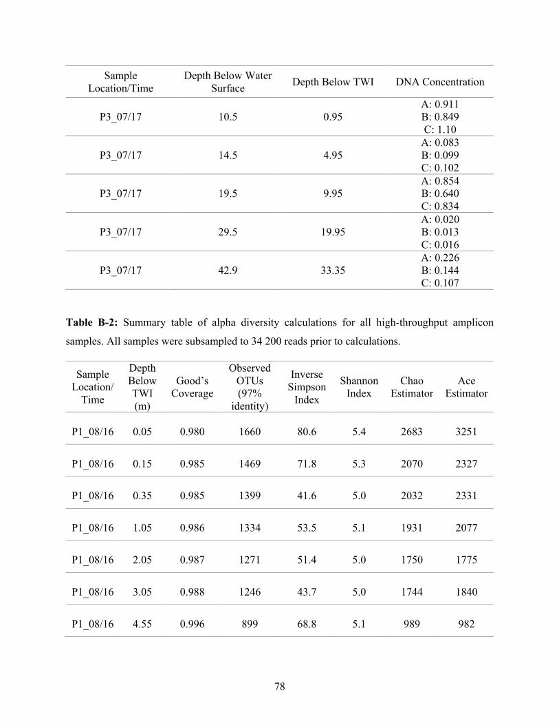
78

Sample Location/Time

Depth Below Water Surface Depth Below TWI DNA Concentration

P3_07/17

10.5

0.95

A: 0.911 B: 0.849 C: 1.10

P3_07/17

14.5

4.95

A: 0.083 B: 0.099 C: 0.102

P3_07/17

19.5

9.95

A: 0.854 B: 0.640 C: 0.834

P3_07/17

29.5

19.95

A: 0.020 B: 0.013 C: 0.016

P3_07/17

42.9

33.35

A: 0.226 B: 0.144 C: 0.107

Table B-2: Summary table of alpha diversity calculations for all high-throughput amplicon

samples. All samples were subsampled to 34 200 reads prior to calculations.

Sample Location/

Time

Depth Below TWI (m)

Good’s Coverage

Observed OTUs (97%

identity)

Inverse Simpson

Index

Shannon Index

Chao Estimator

Ace Estimator

P1_08/16

0.05 0.980 1660 80.6 5.4 2683 3251

P1_08/16

0.15 0.985 1469 71.8 5.3 2070 2327

P1_08/16

0.35 0.985 1399 41.6 5.0 2032 2331

P1_08/16

1.05 0.986 1334 53.5 5.1 1931 2077

P1_08/16

2.05 0.987 1271 51.4 5.0 1750 1775

P1_08/16

3.05 0.988 1246 43.7 5.0 1744 1840

P1_08/16

4.55 0.996 899 68.8 5.1 989 982

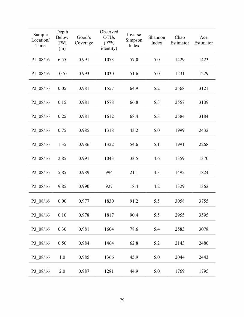
79

Sample Location/

Time

Depth Below TWI (m)

Good’s Coverage

Observed OTUs (97%

identity)

Inverse Simpson

Index

Shannon Index

Chao Estimator

Ace Estimator

P1_08/16

6.55 0.991 1073 57.0 5.0 1429 1423

P1_08/16

10.55 0.993 1030 51.6 5.0 1231 1229

P2_08/16

0.05 0.981 1557 64.9 5.2 2568 3121

P2_08/16

0.15 0.981 1578 66.8 5.3 2557 3109

P2_08/16

0.25 0.981 1612 68.4 5.3 2584 3184

P2_08/16

0.75 0.985 1318 43.2 5.0 1999 2432

P2_08/16

1.35 0.986 1322 54.6 5.1 1991 2268

P2_08/16

2.85 0.991 1043 33.5 4.6 1359 1370

P2_08/16

5.85 0.989 994 21.1 4.3 1492 1824

P2_08/16

9.85 0.990 927 18.4 4.2 1329 1362

P3_08/16

0.00 0.977 1830 91.2 5.5 3058 3755

P3_08/16

0.10 0.978 1817 90.4 5.5 2955 3595

P3_08/16

0.30 0.981 1604 78.6 5.4 2583 3078

P3_08/16

0.50 0.984 1464 62.8 5.2 2143 2480

P3_08/16

1.0 0.985 1366 45.9 5.0 2044 2443

P3_08/16

2.0 0.987 1281 44.9 5.0 1769 1795

80

Sample Location/

Time

Depth Below TWI (m)

Good’s Coverage

Observed OTUs (97%

identity)

Inverse Simpson

Index

Shannon Index

Chao Estimator

Ace Estimator

P3_08/16

4.7 0.988 1142 32.1 4.7 1686 2023

P3_08/16

7.7 0.987 1224 70.4 5.2 1753 2078

P3_08/16

9.7 0.988 1195 58.4 5.0 1657 1781

P1_03/17

0.05 0.979 1705 36.2 5.2 2798 3478

P1_03/17

0.25 0.980 1697 77.0 5.5 2785 3423

P1_03/17

0.35 0.980 1687 92.2 5.6 2750 3346

P1_03/17

1.45 0.984 1424 58.1 5.2 2236 2626

P2_03/17

0.05 0.979 1762 53.5 5.4 2850 3355

P2_03/17

0.15 0.979 1728 99.8 5.6 2814 3476

P2_03/17

0.35 0.983 1470 53.8 5.1 2285 2747

P2_03/17

1.45 0.984 1353 46.7 5.0 2183 2666

P3_03/17

0.05 0.985 1302 35.2 4.8 2100 2564

P3_03/17

0.15 0.985 1243 32.3 4.7 1988 2383

P3_03/17

0.35 0.983 1464 42.5 5.0 2338 2775

P3_03/17

1.35 0.985 1260 33.7 4.8 1986 2486

P1_07/17

0.10 0.977 1891 74.5 5.5 3080 3749

81

Sample Location/

Time

Depth Below TWI (m)

Good’s Coverage

Observed OTUs (97%

identity)

Inverse Simpson

Index

Shannon Index

Chao Estimator

Ace Estimator

P1_07/17

0.20 0.979 1741 90.0 5.6 2909 3659

P1_07/17

1.0 0.984 1395 55.6 5.1 2227 2614

P1_07/17

5.0 0.985 1287 63.1 5.1 2016 2431

P1_07/17

10.0 0.988 1175 45.7 4.9 1611 1650

P1_07/17

20.0 0.986 1123 25.4 4.3 1789 2241

P1_07/17

32.0 0.988 1030 27.4 4.4 1526 1777

P2_07/17

0.05 0.980 1603 55.4 5.2 2658 3265

P2_07/17

0.15 0.983 1383 30.3 4.8 2220 2673

P2_07/17

0.95 0.983 1415 31.7 4.9 2195 2631

P2_07/17

4.75 0.987 1101 16.7 4.4 1692 2064

P2_07/17

9.75 0.986 1180 22.3 4.5 1843 2264

P2_07/17

13.75 0.984 1312 28.7 4.6 2138 2775

P2_07/17

17.75 0.986 1124 14.1 4.1 1872 2355

P3_07/17

0.05 0.976 1912 69.5 5.5 3221 3994

P3_07/17

0.15 0.980 1681 75.4 5.4 2709 3375

P3_07/17

0.95 0.983 1482 57.0 5.1 2387 2876

82

Sample Location/

Time

Depth Below TWI (m)

Good’s Coverage

Observed OTUs (97%

identity)

Inverse Simpson

Index

Shannon Index

Chao Estimator

Ace Estimator

P3_07/17

4.95 0.987 1256 41.8 4.9 1760 1811

P3_07/17

9.95 0.985 1265 48.1 5.0 2049 2500

P3_07/17

19.95 0.993 998 40.2 4.9 1191 1181

P3_07/17

33.35 0.988 1114 39.9 4.7 1638 1999

83

Figure B-1: Dendrogram created using the theta Yue-Clayton index. The labelling is depicted as

the platform location, followed by the date of sample collection and the depth below the TWI in

meters.

P3 07/17 0.15 P1 07/17 0.20 P2 03/17 0.15 P1 03/17 0.25 P1 03/17 0.35 P3 07/17 0.05 P1 07/17 0.10 P3 08/16 0.10 P3 08/16 0.00 P1 08/16 0.05 P2 08/16 0.25 P2 08/16 0.15 P2 08/16 0.05 P2 07/17 0.95 P3 03/17 0.35 P3 03/17 1.35 P3 03/17 0.15 P3 08/16 4.70 P2 08/16 2.85 P1 08/16 0.35 P2 03/17 1.45 P1 08/16 3.05 P1 08/16 2.05 P2 08/16 1.35 P2 07/17 0.15 P3 03/17 0.05 P2 08/16 0.75 P2 07/17 0.05 P2 03/17 0.35 P3 07/17 0.95 P1 03/17 1.45 P1 07/17 1.00 P1 08/16 1.05 P3 08/16 2.00 P3 08/16 1.00 P3 08/16 0.50 P1 08/16 0.15 P3 08/16 9.70 P3 08/16 7.70 P1 08/16 6.55 P3 08/16 0.30 P3 07/17 33.35 P1 07/17 32.0 P1 07/17 20.0 P3 07/17 9.95 P1 07/17 5.00 P1 07/17 10.0 P2 07/17 17.75 P2 07/17 9.75 P2 07/17 4.75 P2 08/16 9.85 P2 08/16 5.85 P2 07/17 13.75 P3 07/17 19.95 P3 07/17 4.95 P1 08/16 10.55 P1 08/16 4.55 P2 03/17 0.05 P1 03/17 0.05

0.1

84

Figure B-2: Dendrogram created using the Jaccard index. The labelling is depicted as the platform

location, followed by the date of sample collection and the depth below the TWI in meters.

P3 07/17 0.15 P1 07/17 0.20 P2 03/17 0.15 P1 03/17 0.25 P1 03/17 0.35 P3 08/16 0.30 P3 07/17 0.95 P1 07/17 1.00 P1 03/17 1.45 P3 08/16 2.00 P1 08/16 1.05 P3 08/16 0.50 P3 08/16 1.00 P1 08/16 0.15 P2 07/17 0.95 P2 03/17 1.45 P2 03/17 0.35 P1 08/16 0.35 P2 08/16 1.35 P2 08/16 0.75 P2 07/17 0.15 P3 03/17 0.35 P3 03/17 1.35 P3 03/17 0.15 P3 03/17 0.05 P2 07/17 0.05 P3 07/17 0.05 P1 07/17 0.10 P3 08/16 0.10 P3 08/16 0.00 P2 08/16 0.25 P2 08/16 0.15 P2 08/16 0.05 P1 08/16 0.05 P2 03/17 0.05 P1 03/17 0.05 P3 07/17 33.35 P1 07/17 32.0 P1 07/17 20.0 P3 07/17 19.95 P1 07/17 10.0 P1 08/16 10.55 P3 07/17 4.95 P3 07/17 9.95 P1 07/17 5.00 P3 08/16 9.70 P3 08/16 7.70 P1 08/16 6.55 P3 08/16 4.70 P2 08/16 2.85 P1 08/16 3.05 P1 08/16 2.05 P2 07/17 17.75 P2 07/17 4.75 P2 08/16 9.85 P2 08/16 5.85 P2 07/17 13.75 P2 07/17 9.75 P1 08/16 4.55

0.050