geometric interpolation by planar parametric polynomial curves
TRANSCRIPT

UNIVERSITY OF LJUBLJANA
FACULTY OF MATHEMATICS AND PHYSICS
DEPARTMENT OF MATHEMATICS
Marjetka Krajnc
GEOMETRIC INTERPOLATION BY PLANAR
PARAMETRIC POLYNOMIAL CURVES
Doctoral thesis
ADVISER: Prof. Dr. Jernej Kozak
Ljubljana, 2008


UNIVERZA V LJUBLJANI
FAKULTETA ZA MATEMATIKO IN FIZIKO
ODDELEK ZA MATEMATIKO
Marjetka Krajnc
GEOMETRIJSKA INTERPOLACIJA
Z RAVNINSKIMI PARAMETRICNIMI
POLINOMSKIMI KRIVULJAMI
Doktorska disertacija
MENTOR: Prof. Dr. Jernej Kozak
Ljubljana, 2008


Zahvala
Zahvaljujem se mojemu mentorju prof. dr. Jerneju Kozaku, ki je ves cas verjel vame,me spodbujal in mi dajal neprecenljive nasvete. Brez njegovih izjemnih idej disertacijagotovo ne bi bila taksna kot je.
Hvala sodelavcem Gasperju, Emilu in Vitu za pozoren pregled mojih clankov in vsekoristne nasvete ter spodbudne besede. Delo z vami je res prijetno.
Zahvaljujem se tudi clanom seminarja za Numericno matematiko, ker so me takolepo sprejeli medse in z zanimanjem poslusali moja predavanja. Hvala prof. dr. PetruSemrlu, ki mi je omogocil mesto mlade raziskovalke na IMFM ter vsem ostalim, ki so nakakrsenkoli nacin pripomogli k tej disertaciji.
Beseda zahvale gre tudi mojim starsem, ki so mi omogocili studij in mi ves cas stali obstrani. Predvsem pa hvala Borisu in sinu Davidu za vso njuno potrpezljivost, ljubezen,smeh in veselje, ki ga vnasata v moje zivljenje.
iii


Abstract
In the thesis the geometric interpolation by planar parametric polynomial curves isconsidered. In the introduction general geometric interpolation schemes, their propertiesand advantages are outlined, and main results about these schemes are presented. TheLagrange problem of interpolating 2n points in the plane by a polynomial curve of degreen is considered in detail. Since the problem is nonlinear, the question of the existenceof the solution is very difficult. In Chapter 2, sufficient geometric conditions that ensurethe existence of the cubic curve that interpolates six points in the plane are given.The conditions turn out to be quite simple and depend only on certain determinantsderived from data points. The results cover convex and nonconvex data. In the nextchapter the geometric interpolation by cubic G1 spline curves is considered. Sufficientgeometric conditions are derived that admit the existence of a G1 spline curve, where oneach polynomial segment four points and two tangent directions are interpolated. Analgorithm that determines the areas for tangent directions, such that the existence ofthe spline is guaranteed, is presented. In Chapter 4 the Hermite geometric interpolationby cubic polynomial curves is studied. Again, sufficient geometric conditions are derivedthat cover most of the cases. From the analysis of geometric interpolation by cubiccurves it is clear that it would be impossible to consider the problem for a general degreewithout some further assumptions. In Chapter 5 the asymptotic approach is applied,which means that the data are sampled from a smooth convex curve f : [0, h] → R2 withh small enough. For a general degree n a special nonlinear system of equations is derivedand it is proven that in the case that it has at least one real solution the approximationorder is optimal, i.e., 2n. The existence of the solution of this system is proven for n ≤ 5for general curves. For a general degree n the existence of the solution is established fora special class of functions, so called circle-like curves. Tools used in the analysis areresultants, Grobner basis and Brouwer’s mapping degree. Their definitions and mainproperties are given in the last chapter.
Key-words: geometric interpolation, polynomial curve, spline curve, geometric conti-nuity, existence of the solution, parametric distance, asymptotic analysis, approximationorder, CAGD.
Math. Subj. Class. (2000): 65D05, 65D07, 65D10, 65D17.
v


Povzetek
V disertaciji je obravnavana geometrijska interpolacija z ravninskimi parametricnimipolinomskimi krivuljami. V uvodu so predstavljene splosne geometrijske interpolacijskesheme, njihove glavne lastnosti in prednosti. Podani so najpomembnejsi rezultati s tegapodrocja. Podrobno je predstavljen Lagrangeev problem interpolacije 2n ravninskih tocks polinomsko krivuljo stopnje n. Ker je problem nelinearen, je vprasanje o obstoju resitveprecej tezko. V drugem poglavju so izpeljani geometrijski pogoji, ki zagotavljajo obstojkubicne interpolacijske krivulje, ki interpolira sest tock v ravnini. Pogoji so preprostopreverljivi in odvisni le od geometrije danih tock. Rezultati pokrijejo tako konveksnekot nekonveksne podatke. V naslednjem poglavju je obravnavan problem geometrijskeinterpolacije s kubicnimi G1 zlepki. Izpeljani so zadostni pogoji za obstoj G1 zlepka, kjerso na vsakem odseku interpolirane stiri tocke in dve smeri tangent. Dodan je algoritem,s katerim dolocimo obmocja za smeri tangent, da je obstoj zlepka zagotovljen. V cetrtempoglavju je obravnavana Hermitova interpolacija s kubicnimi polinomskimi krivuljami inG1 zlepki. Izpeljani so geometrijski pogoji, ki zagotavljajo obstoj interpolanta, ki pokri-jejo vecino primerov. Iz analize problema interpolacije s kubicnimi polinomi se vidi, daje v splosnem problem nemogoce obravnavati brez kaksnih dodatnih predpostavk. Vpetem poglavju je uporabljen asimptoticni pristop, kar pomeni, da so podatki vzeti izgladke konveksne krivulje f : [0, h] → R
2, kjer je h dovolj majhen. Za poljubno stopnjon je izpeljan poseben sistem nelinearnih enacb in dokazano je, da je v primeru, ko imata sistem vsaj eno realno resitev, red aproksimacije optimalen, to je 2n. Obstoj resitvetega sistema je za poljubne krivulje dokazan za stopnje n ≤ 5. Za poljubne stopnje poli-nomov pa je obstoj resitve dokazan za poseben razred krivulj, tako imenovane krivuljeblizu kroznice. V dokazih so uporabljene rezultante, Grobnerjeve baze in Brouwerjevastopnja. Njihove definicije in glavne lastnosti so podane v zadnjem poglavju.
Kljucne besede: geometrijska interpolacija, polinomska krivulja, krivulja zlepkov,geometrijska zveznost, obstoj resitve, parametricna razdalja, asimptoticna analiza, redaproksimacije, CAGD.
Math. Subj. Class. (2000): 65D05, 65D07, 65D10, 65D17.
vii


Contents
1 Introduction 1
2 Geometric interpolation by cubic polynomials 92.1 The main results . . . . . . . . . . . . . . . . . . . . . . . . . . . . . . . 92.2 The equations . . . . . . . . . . . . . . . . . . . . . . . . . . . . . . . . . 132.3 Proof of Theorem 2.4 . . . . . . . . . . . . . . . . . . . . . . . . . . . . . 142.4 A particular case . . . . . . . . . . . . . . . . . . . . . . . . . . . . . . . 182.5 Proofs of main theorems . . . . . . . . . . . . . . . . . . . . . . . . . . . 202.6 Examples . . . . . . . . . . . . . . . . . . . . . . . . . . . . . . . . . . . 21
3 Geometric interpolation by cubic G1 splines 253.1 Interpolation problem . . . . . . . . . . . . . . . . . . . . . . . . . . . . . 253.2 Polynomial case . . . . . . . . . . . . . . . . . . . . . . . . . . . . . . . . 273.3 Proof of Theorem 3.6 and Theorem 3.7 . . . . . . . . . . . . . . . . . . . 323.4 The G1 spline curve . . . . . . . . . . . . . . . . . . . . . . . . . . . . . . 383.5 Examples . . . . . . . . . . . . . . . . . . . . . . . . . . . . . . . . . . . 48
4 Hermite geometric interpolation by cubic G1 splines 554.1 Interpolation problem . . . . . . . . . . . . . . . . . . . . . . . . . . . . . 554.2 Single segment case . . . . . . . . . . . . . . . . . . . . . . . . . . . . . . 584.3 Relations, implying the solution to approach the boundary . . . . . . . . 604.4 Main theorems . . . . . . . . . . . . . . . . . . . . . . . . . . . . . . . . 644.5 Proofs of main theorems . . . . . . . . . . . . . . . . . . . . . . . . . . . 664.6 Approximation order . . . . . . . . . . . . . . . . . . . . . . . . . . . . . 70
5 Asymptotic analysis 755.1 Asymptotic approach . . . . . . . . . . . . . . . . . . . . . . . . . . . . . 755.2 Nonlinear system . . . . . . . . . . . . . . . . . . . . . . . . . . . . . . . 765.3 System of equations in asymptotic form . . . . . . . . . . . . . . . . . . . 775.4 The case n = 4. . . . . . . . . . . . . . . . . . . . . . . . . . . . . . . . . 835.5 The case n = 5. . . . . . . . . . . . . . . . . . . . . . . . . . . . . . . . . 87
6 Circle-like curves 936.1 Circle-like curves . . . . . . . . . . . . . . . . . . . . . . . . . . . . . . . 936.2 Interpolation problem . . . . . . . . . . . . . . . . . . . . . . . . . . . . . 946.3 The main results . . . . . . . . . . . . . . . . . . . . . . . . . . . . . . . 97
ix

6.4 Proofs . . . . . . . . . . . . . . . . . . . . . . . . . . . . . . . . . . . . . 1016.5 Approximation of circular arcs . . . . . . . . . . . . . . . . . . . . . . . . 105
7 Resultants, Grobner basis and Brouwer’s degree 1097.1 Resultants . . . . . . . . . . . . . . . . . . . . . . . . . . . . . . . . . . . 1097.2 Grobner basis . . . . . . . . . . . . . . . . . . . . . . . . . . . . . . . . . 1107.3 Brouwer’s mapping degree . . . . . . . . . . . . . . . . . . . . . . . . . . 111
Bibliography 113
Index 117
Razsirjeni povzetek 119
x

Chapter 1
Introduction
The geometric interpolation by parametric polynomial curves has received considerableattention since it was introduced in [4], where a Hermite cubic interpolation of two points,tangent directions and curvatures is studied. It was shown that under some natural re-strictions a planar convex curve can be approximated up to the sixth order accuracy.High approximation order is one of the reasons for a further work on the subject. Theother is the fact that geometric interpolants in many cases please the human eye morethan their usual standard counterparts. The underlying basic concept of geometric inter-polation is to consider the curve itself independent of its actual parameterization. Theinterpolating curve depends only on geometric quantities such as data points, tangentdirections, curvatures, etc. This makes the geometric interpolant a valuable tool in thecomputer aided geometric design. No additional artificial conditions are imposed on thecurve such as at which parameter values the interpolation conditions should be met.Since no free parameters are used ineffectively, geometric interpolation often results inhigher approximation order than one would expect from the functional case.
But, unfortunately, geometric interpolating schemes involve a nonlinear part. Thisdrawback makes it hard to analyse the existence of the interpolating curve and to estab-lish the approximation order. Numerical computations have to be done with some caretoo, usually by the continuation method ([2]). Thus it is quite clear why the analysisof geometric interpolation schemes is usually based upon the assumption that data aresampled densely enough from a smooth curve, and the asymptotic analysis is applied.
Commonly, a curve is not approximated by a single polynomial or rational curve,but by a geometric spline, i.e., a finite number of consecutive segments, joining at thebreakpoints with an appropriate order of geometric continuity. Two curves join withG0 continuity if they meet at a common join point, with G1 continuity if they share acommon tangent direction at the join point, and with G2 continuity if additionally thesigned curvature at the join point is continuous. In general, geometric continuity can bedefined in the following way.
DEFINITION 1.1. Two parametric curves
fffffffff1 : [t0, t1] → Rd, fffffffff 2 : [s0, s1] → R
d,

2 Introduction
join with a geometric continuity of order k or shortly with Gk-continuity if the end pointof fffffffff 1 coincides with the starting point of fffffffff 2, fffffffff 1(t1) = fffffffff2(s0), and there exists a regularreparameterization φ : [t0, t1] → [s0, s1] such that
djfffffffff 1
dtj(t)
∣∣∣∣t=t1
=dj(fffffffff 2 ◦ φ)
dtj(t)
∣∣∣∣t=t1
, j = 0, 1, . . . , k.
In order to study the approximation order in parametric case we need to know how tomeasure the distance between parametric objects. Since objects are usually consideredas sets of points the well known Hausdorff distance dH is one of the possible metrics. Itis defined in the following way.
DEFINITION 1.2. Let X and Y be two subsets of a metric space M . The Hausdorffdistance dH(X, Y ) is defined by
dH(X, Y ) := max
{
supx∈X
infy∈Y
d(x, y), supy∈Y
infx∈X
d(x, y)
}
,
where d(x, y) is a metric on M .
But unfortunately, it is difficult to compute the Hausdorff distance in practice. Asits upper bound the so called parametric distance dP has been proposed by Lyche andMørken ([34]).
DEFINITION 1.3. Let fffffffff 1 and fffffffff 2 be two parametric curves defined on intervals I1 andI2, respectively. The parametric distance between fffffffff1 and fffffffff 2 is defined by
dist(fffffffff 1, fffffffff 2) := infφ‖fffffffff1 ◦ φ− fffffffff 2‖ = inf
φmaxt∈I2
‖fffffffff 1(φ(t)) − fffffffff 2(t)‖,
where φ : I2 → I1 is a regular reparameterization, i.e., φ′ 6= 0 on I2.
Let us now summarize some of the well known results on geometric interpolation.In [4], C. de Boor, K. Hollig, and M. Sabin introduce the concept of geometric conti-nuity. They study the approximation of a curve fffffffff : R → R2 by planar piecewise cubicpolynomials. Data points, tangent directions and curvatures of fffffffff at given nodes ti areinterpolated. The authors show that for h := supi ‖fffffffff(ti+1) − fffffffff(ti)‖ sufficiently small aninterpolant which approximates fffffffff at the surprisingly high order h6 exists, except whenthe curvature of fffffffff vanishes. Then the approximation order is locally reduced to h4.They also show that the interpolant need not be unique.
In [22], K. Hollig and J. Koch make the following conjecture.
CONJECTURE 1.4. Under appropriate generic assumptions, a polynomial curve ofdegree n can interpolate
m = n+ 1 +
⌊n− 1
d− 1
⌋
points on a smooth curve fffffffff ∈ Rd. This interpolant approximates fffffffff with order m as thedistance of interpolation points tends to zero.
3
They give a proof of this conjecture for planar quadratic polynomial and spline curvesand describe a simple construction of curvature continuous quadratic splines from controlpolygons. In [21], the same two authors consider the approximation of space curves bycubic splines and prove that a smooth space curve can be approximated by a cubicpolynomial with fifth-order accuracy at any point where the curvature and torsion donot vanish. They describe a natural generalization of the standard Hermite interpolationwhich achieves the optimal approximation order 5 for degree 3. In addition to the positionand the tangent direction at the endpoints, a third point within the parameter intervalis interpolated.
In [37], K. Mørken and K. Scherer establish a general framework for geometric in-terpolation methods for parametric curves that includes interpolation methods in alldimensions. Questions of solvability and stability are considered. As a special case ofthe general result, they prove that four points on a planar curve can be interpolatedby a quadratic with fourth-order accuracy, if the points are sufficiently close to a pointwith a nonvanishing curvature. They also prove that six points on a planar curve canbe interpolated by a cubic with sixth-order accuracy, provided the points are sufficientlyclose to a point where the curvature does not have a double zero. In space it turns outthat five points sufficiently close to a point with nonvanishing torsion can be interpolatedby a cubic, with fifth-order accuracy. The case of quartic curves in the plane is studiedby K. Scherer in [45] and [46].
In [34], T. Lyche and K. Mørken define a metric on the set of parametric curves(see Definition 1.3). They give a definition of approximation rate for parametric ap-proximation schemes in terms of this metric, and present a simple family of odd degreeparametric polynomial approximations to circle segments with the approximation ordertwice the degree of the polynomial.
Degen ([7]) extends the work of C. de Boor, K. Hollig, and M. Sabin ([4]). Heshows, by using rational cubics, that it is possible to have third-order contact at theendpoints, which raises the approximation order to eight. Analysing the solvabilityconditions for third-order contact by rational cubics he establishes that purely geometricproperties of the given curve determine whether the desired approximant exists. In[8] Degen introduces the notion of geometric contact elements and designs a unifiedtheory of geometric Hermite interpolation for parametric curves. He predicts the order ofapproximation to be 2n for a polynomial curve and 3n− 1 for a rational curve of degreen. In his recent work [9] Degen presents an excellent overview of the developmentsof geometric Hermite approximation theory for planar curves. A general method tosolve these problems is presented. Geometric interpretations, examples and a detaileddiscussion of the case of degree n = 4 with one contact point is given.
In [38], Rababah describes a Taylor polynomial interpolation for space curves whichyields the order (n+ 1) +
[n+12d−1
]for a curve in Rd, where n is the degree of the approx-
imating polynomial curve. The cubic case is studied with examples. He extends theseresults to the piecewise polynomial curve interpolation in [39].
An important contribution to the subject is given by J. Kozak, Y. Y. Feng andE. Zagar ([16], [15], [14], [26], [27], [28], [47]). In [16] the interpolation by G2 continuousBezier spline curves in Rd is outlined. Each segment of the spline curve interpolatesr interior and two boundary points. A general approach is followed in detail for the
4 Introduction
case d = 3, n = 3, r = 1. For the single component case, the optimal approximationorder is proved, and asymptotic existence established. In [15] the interpolation by G2
continuous planar cubic Bezier spline curves is studied. The interpolation is based onlyon the underlying curve points and the end tangent directions. On each polynomialsegment four points and two tangent directions are interpolated. The authors show theexistence of the interpolant in asymptotic sense and prove that the approximation orderis optimal. In [47], E. Zagar considers an interpolation by G2 spline curves of degree din R
d that interpolate d points on each segment. He shows that if the data points aresampled regularly and are sufficiently dense, then the interpolant exists. The optimalapproximation order d+ 2 is achieved.
Results on rational and polynomial geometric interpolation by R. Schaback can befound in [40], [41], [44], [42], and [43].
Most of the mentioned results are obtained by the asymptotic approach. However,results offered by the asymptotic analysis are not always adequate in practical applica-tions. If one is merely looking for an interpolant of a nice shape, suppositions like ”if datapoints are sampled dense enough” are not very encouraging. Therefore robust algorithmsshould be based upon conditions that ensure the existence in advance if possible at all.But in geometric interpolation, this can be rarely achieved. Beside some special cases,like the interpolation of a circle ([34] [10], [19] [35], [17], [18], [11], [12]), there are onlyfew results concerning geometric conditions for the existence of the interpolant. Theinterpolation by a parametric parabola at four distinct planar points is studied in [33],where the conditions are established through geometric arguments. In [36] the algebraicapproach is applied, and results are extended to all possible cases (Taylor, Hermite, La-grange). The interpolation of an arbitrary number of points in a plane with compositeG2 quadratic curves is studied in [41], [14], [26], where sufficient conditions for solvabil-ity and the uniqueness of the solution are derived. Perhaps the most general resultsare given by J. Kozak and E. Zagar in [27], where necessary and sufficient geometricconditions for the simplest nontrivial geometric interpolation schemes in all dimensions,i.e., the interpolation of d+ 2 distinct points in R
d by a polynomial curve of degree ≤ d,are outlined.
In this thesis the study of geometric interpolation is restricted to the planar cased = 2. Planar schemes are probably the most important in practice, and the gapbetween the parametric and the functional case is the largest. Namely, Conjecture 1.4states that 2n planar points can be interpolated by a polynomial curve of degree n, andthe approximation order 2n can be achieved, while in the functional case a polynomialof degree n can interpolate only n+ 1 points with the approximation order n+ 1.
The Lagrange interpolation problem considered is the following. For 2n given datapoints
TTTTTTTTT 0, TTTTTTTTT 1, . . . , TTTTTTTTT 2n−1 ∈ R2, TTTTTTTTT i 6= TTTTTTTTT i+1, (1.1)
find a parametric polynomial curve
PPPPPPPPP n : [t0, t2n−1] → R2
of degree ≤ n that interpolates these points at some values ti in an increasing order,
t0 < t1 < · · · < t2n−2 < t2n−1. (1.2)

5
Since a linear transformation of the parameter preserves the degree of a parametricpolynomial curve, one can assume t0 := 0 and t2n−1 := 1, but the remaining parameters
ttttttttt := (ti)2n−2i=1
are unknown. The admissible parameters ti can be viewed as components of a point inthe open simplex
Dn :={(ti)
2n−2i=1 ; 0 = t0 < t1 < · · · < t2n−2 < t2n−1 = 1
},
with the boundary ∂Dn where at least two different ti coincide. The system of equations
PPPPPPPPP n(ti) = TTTTTTTTT i, i = 0, 1, . . . , 2n− 1, (1.3)
should determine the unknown PPPPPPPPP n as well as the parameters ttttttttt. Once the parameters aredetermined it is straightforward to obtain the coefficients of the polynomial curve PPPPPPPPP n.One only has to take any n+ 1 distinct interpolating conditions in (1.3), and apply anystandard interpolation scheme like Newton or Lagrange componentwise.
Since the system (1.3) is nonlinear, it is usually difficult to prove the existence of asolution. Also, a solution does not necessary exist. As a simple example take four points(n = 2) with a nonconvex data polygon. Since each component of the interpolating PPPPPPPPP 2
is a parabola and since a parabola cannot have more than two zeros it is clear that theinterpolant can not exist. But for this case very nice necessary and sufficient conditionsfor the existence are given in [27]. Namely, the interpolant PPPPPPPPP 2 exists if and only ifdeterminants
det (∆TTTTTTTTT 0,∆TTTTTTTTT 1), det (∆TTTTTTTTT 0,∆TTTTTTTTT 2), det (∆TTTTTTTTT 1,∆TTTTTTTTT 2),
where ∆TTTTTTTTT i := TTTTTTTTT i+1 − TTTTTTTTT i, are of the same sign.As a motivation to geometric interpolation schemes let us consider some numerical
examples. First, let us compare the cubic geometric scheme with a componentwisequintic interpolation, where a parameterization is chosen in advance as the uniform,
t0 = 0, ti+1 = ti + 1,
and the chord length parameterization,
t0 = 0, ti+1 = ti + ‖TTTTTTTTT i+1 − TTTTTTTTT i‖.
The cubic curve (black) clearly does the job much better than its quintic counterpartsas one can observe in Figure 1.1. The shape of the geometric interpolation curve is asone would require for the given data points, without any visible extraneous inflections.Also, the computational effort to compute these six cubic interpolants turns out to benegligible. The Newton method with equidistant starting values ti = i
5converges within
a machine precision accuracy in eight iterations on average. There is perhaps a simpleexplanation of the fact that the cubic geometric interpolation curves are superior. Anapproximate curvature, with denominator neglected, is a parabola
det(
PPPPPPPPP 3, PPPPPPPPP 3
),

6 Introduction
T0
T1
T2T3
T4
T5 T0
T1
T2 T3
T4
T5T0
T1
T2 T3
T4
T5
T0
T1
T2
T3
T4
T5
T0
T1T2
T3
T4
T5
T0 T1
T2
T3
T4T5
Figure 1.1: A geometric cubic interpolant (black) and quintic polynomial interpolatingcurves with uniform (grey) and chord length parameterization (dashed).
so the rate of change of the curvature is approximately linear what pleases most thehuman eye.
As a next example let us approximate a particular logaritmic spiral
fffffffff(t) = log (t+ π)
(sin tcos t
)
, t ∈[
−π2,π
2
]
, (1.4)
by geometric interpolants of degrees n = 3, 4, 5, 6. The data points are obtained from(1.4) by the equidistant splitting of the parameter domain. Table 1.1 numerically sug-gests that the approximation order is 2n, where the error is measured as the parametricdistance between the curve and its interpolants.
The outline of the thesis is the following. In Chapter 2 the geometric conditionsthat imply the existence of a cubic geometric interpolant that interpolates six points inthe plane are presented. The conditions depend only on certain determinants of datapoints and are very simple to verify. The results cover both the convex and nonconvex

7
Interval Approximation error Decay exponentn = 3 n = 4 n = 3 n = 4
[−π
2, π
2
]2.2662 × 10⁻² 1.6485 × 10⁻³ — —
[−5π
12, 5π
12
]8.0154 × 10⁻³ 3.6922 × 10⁻⁴ 5.70 8.21
[−4π
12, 4π
12
]2.1793 × 10⁻³ 5.8837 × 10⁻⁵ 5.84 8.23
[−3π
12, 3π
12
]3.9573 × 10⁻⁴ 5.5716 × 10⁻⁶ 5.93 8.19
[−2π
12, 2π
12
]3.4941 × 10⁻⁵ 2.0533 × 10⁻⁷ 5.99 8.14
[− π
12, π
12
]5.4085 × 10⁻⁷ 7.5616 × 10⁻¹⁰ 6.01 8.09
n = 5 n = 6 n = 5 n = 6[−π
2, π
2
]5.0251 × 10⁻⁵ 1.7288 × 10⁻⁷ — —
[−5π
12, 5π
12
]7.7733 × 10⁻⁶ 2.3347 × 10⁻⁸ 10.24 10.98
[−4π
12, 4π
12
]7.7842 × 10⁻⁷ 2.1547 × 10⁻⁹ 10.31 10.68
[−3π
12, 3π
12
]4.0522 × 10⁻⁸ 8.1861 × 10⁻¹¹ 10.27 11.37
[−2π
12, 2π
12
]6.4814 × 10⁻¹⁰ 6.6848 × 10⁻¹³ 10.20 11.86
[− π
12, π
12
]5.8338 × 10⁻¹³ 1.6306 × 10⁻¹⁶ 10.12 12.00
Table 1.1: The error and approximation order in interpolation of the logaritmic spiral(1.4) by geometric interpolants.
data. Chapter 3 extends the results to geometric interpolation by cubic G1 splines.Geometric conditions that imply the existence of a spline are derived, where on eachsegment four points and two tangent directions are interpolated. The conditions againdepend only on positions of data. The algorithm that carries out the verification is added.In the next chapter Hermite interpolation of three points and three tangent directions isconsidered. Geometric conditions for the existence of the interpolant are given and theoptimal approximation order is confirmed. In Chapter 5 the asymptotic analysis is donefor all degrees n. This means that the data are sampled from a smooth convex curvef : [0, h] → R2, with h small enough. The Conjecture 1.4 is proven for degree n ≤ 5. Fora general n, a special nonlinear system of equations is derived and it is proven that inthe case when this system has one real solution, the approximation order is optimal, i.e.,2n. The proof of the existence of a real solution is very difficult. In the proof for degreen = 5 the theory of resultants, Grobner basis, varieties and ideals is used. Chapter 6 isa continuation of the previous one, where the conjecture is proven for a special class offunctions, so called circle-like curves, for general degrees of polynomials.
The results of this thesis are published in the following papers: [29], [30], [31], [23],[24], and [25].


Chapter 2
Geometric interpolation by cubicpolynomials
In this chapter the Lagrange interpolation of six points in R2 by a cubic polynomialcurve is studied. Namely, the interpolation problem introduced in the first chapter ishere considered for n = 3 and simple sufficient geometric conditions that ensure theexistence of the interpolant are given. The conditions turn out to be quite simple anddepend only on certain determinants derived from the data points.
2.1. The main results
The conditions that imply the nonlinear system
PPPPPPPPP 3(ti) = TTTTTTTTT i, i = 0, 1, . . . , 5, (2.1)
to have at least one admissible solution, i.e.,
0 =: t0 < t1 < · · · < t5 := 1, (2.2)
will be determined here. The key role is played by the matrix of data differences,
(∆TTTTTTTTT i
)4
i=0∈ R
2×5,
and by the signs and ratios of its minors
Di,j := det (∆TTTTTTTTT i,∆TTTTTTTTT j). (2.3)

10 Geometric interpolation by cubic polynomials
These are the volumes of parallelograms spanned by the vectors ∆TTTTTTTTT i,∆TTTTTTTTT j . Let us define
λ1 :=D0,1
D1,2, λ2 :=
D0,2
D1,2, λ3 :=
D2,4
D2,3, λ4 :=
D3,4
D2,3, δ :=
D1,3
D1,2, µ :=
D2,3
D1,2,
γ1 :=λ2(1 + λ2)
λ1(1 + λ2) +√
λ1(1 + λ2)(λ1 + λ2),
γ2 :=λ3(1 + λ3)
λ4(1 + λ3) +√
λ4(1 + λ3)(λ3 + λ4).
Note that the data points with a convex control polygon, as in the first three figures ofFigure 1.1, have µ > 0 and λi > 0, i = 1, 2, 3, 4. The control polygons of data pointsin the last three figures of Figure 1.1 change from convexity to concavity at ∆TTTTTTTTT 2. Suchdata have λi > 0 and µ < 0. We will restrict our study to these two types of data.Geometric interpretation of λi, δ and µ is shown in Figure 2.1.
DT0
DT1
DT2
DT3
DT4
∆>0∆<0
Λ1>0Λ2>0
Λ3>0Λ4>0
DT0
DT1
DT2
DT3
DT4
∆>0
∆<0
Λ1>0Λ2>0
Convex data Nonconvex data
Figure 2.1: Geometric interpretation of λi, δ and µ for convex and nonconvex data.
Further let us define λλλλλλλλλ := (λi)4i=1, and the functions
ϑ1 (λλλλλλλλλ, µ) :=2µ− γ1 +
√
γ21 + 4µ(1 + γ1)
2γ1,
ϑ2 (λλλλλλλλλ, µ) :=2 − µγ2 +
√
µ2γ22 + 4µ(1 + γ2)
2γ2,
ϑ3 (λλλλλλλλλ, µ) :=λ1µ
λ2+λ4
λ3+µ
λ2
√
λ1(λ1 + λ2)
1 + λ2,
ϑ4 (λλλλλλλλλ, µ) :=λ1µ
λ2+λ4
λ3+
1
λ3
√
λ4(λ3 + λ4)
1 + λ3,
that will be used in boundary relations between the constants, that ensure the existenceof the solution. The main results are the following.

2.1 The main results 11
THEOREM 2.1. Suppose that D1,2D2,3 6= 0 and the data are convex, i.e., µ > 0 andλi > 0, i = 1, 2, 3, 4. If either ϑ1 (λλλλλλλλλ, µ) = ϑ2 (λλλλλλλλλ, µ), or one of the following conditions ismet,
δ < minℓ=1,2
{ϑℓ (λλλλλλλλλ, µ)} or δ > maxℓ=1,2
{ϑℓ (λλλλλλλλλ, µ)} ,
then the cubic interpolating curve PPPPPPPPP 3 that satisfies (2.1) exists.
THEOREM 2.2. Suppose that D1,2D2,3 6= 0, and the data imply an inflection point,i.e., µ < 0 and λi > 0, i = 1, 2, 3, 4. If
δ ∈ (ϑ3(λλλλλλλλλ, µ), ϑ4(λλλλλλλλλ, µ)) ,
then the cubic interpolating curve PPPPPPPPP 3 that satisfies (2.1) exists.
Theorem 2.1 and Theorem 2.2 provide only sufficient conditions for the existence ofa cubic geometric interpolant. But the next conclusion excludes most of the data thatdo not satisfy these two theorems.
THEOREM 2.3. The cases where the solution of the interpolation problem (2.1) doesnot exist are summarized in Table 2.1.
D1,2D2,3 6= 0 D1,2D2,3 = 0µ > 0 µ < 0
λ2 ≤ 0, λ3 ≤ 0 λ2 ≤ 0 D1,2 = 0, D2,3 = 0δ ≤ 0, λ1 ≤ 0 λ3 ≤ 0 D1,2 = 0, λ3 ≤ 0δ ≤ 0, λ4 ≤ 0 λ1 ≤ 0, δ ≤ 0 D2,3 = 0, λ2 ≤ 0
λ1 ≤ 0, λ3 ≤ 0 , λ4 ≥ 0 λ4 ≤ 0, δ ≥ 0 D1,2 = 0, D0,1D2,3 ≥ 0λ2 ≤ 0, λ4 ≤ 0, λ1 ≥ 0 D2,3 = 0, D1,2D3,4 ≥ 0
Table 2.1: The cases where the solution of the interpolation problem (2.1) does not exist.
Some possibilities are not covered by Theorem 2.1, Theorem 2.2 or Theorem 2.3. Asan example, consider the points
TTTTTTTTT 0 =
(−20 − ξ
3
)
, TTTTTTTTT 1 =
(−101
)
, TTTTTTTTT 2 =
(−50
)
, (2.4)
TTTTTTTTT 3 =
(50
)
, TTTTTTTTT 4 =
(101
)
, TTTTTTTTT 5 =
(20 + ξ
3
)
, ξ > 0,
with λ1 = λ4 = − ξ10
, λ2 = λ3 = 2, δ = µ = 1. Note that neither the requirements ofTheorem 2.1, Theorem 2.2 nor of Theorem 2.3 are met. Now, the data (2.4) admit twosolutions for ξ ∈ (0, ξ0], where ξ0 := 2.95373852 (Figure 2.2). For ξ = ξ0 both of thesolutions coincide with a cusp, but for ξ > ξ0 no solution can be found.
The examples in Figure 1.1 all satisfy the conditions of Theorem 2.1 or of Theorem 2.2.Let us look at two of them more precisely. In the first one δ < ϑ1 (λλλλλλλλλ, µ). Figure 2.3(left) shows how the positions of points change as δ approaches ϑ1 (λλλλλλλλλ, µ). For δ ∈

12 Geometric interpolation by cubic polynomials
T0
T1
T2 T3
T4
T5 T0
T1
T2 T3
T4
T5
T0
T1
T2 T3
T4
T5 T0
T1
T2 T3
T4
T5
Figure 2.2: Four cubic geometric interpolants at points (2.4), with ξ = 2, 2.5, 2.8, ξ0.
[ϑ1 (λλλλλλλλλ, µ) , ϑ2 (λλλλλλλλλ, µ)] no proper solution exists. Similarly, Figure 2.3 (right) shows thedisplacement of points as δ changes from ϑ3 (λλλλλλλλλ, µ) to ϑ4 (λλλλλλλλλ, µ) for the last example ofFigure 1.1. For δ < ϑ3 (λλλλλλλλλ, µ) or δ > ϑ4 (λλλλλλλλλ, µ) two solutions ttttttttt ∈ D3 were found and theproblem similar as in the example above has happened.
T0
T1
T2T3
T4
T5
T0 T1
T2
T3
T4T5
Figure 2.3: The change of point positions as δ approaches ϑ1 (λλλλλλλλλ, µ) (left), and as δchanges from ϑ3 (λλλλλλλλλ, µ) to ϑ4 (λλλλλλλλλ, µ) (right).
The requirements of Theorem 2.1 and Theorem 2.2 are quite simple, but the prooftakes several steps. First, the system (2.1) is transformed into a form more suitable forfurther analysis. Then it is proved that any solution of (2.1) satisfying (2.2) cannot havethe parameters ti arbitrary close to the boundary ∂D3. For particular data it is provedthat the nonlinear system has an odd number of solutions and then this fact is extendedto a general case by a convex homotopy and Brouwer’s degree argument.

2.2 The equations 13
2.2. The equations
First let us split (2.1) into the nonlinear system for unknown parameters only. Thedivided difference [tℓ, tℓ+1, . . . , tℓ+4], applied to the system (2.1), maps any PPPPPPPPP 3 to zero.Let
ωi,j(t) := (t− ti)(t− ti+1) · · · (t− tj−1)(t− tj), ωi,j(t) =d
dtωi,j(t), i < j. (2.5)
Since ti are assumed to be distinct, one can express the divided difference in terms ofωℓ,ℓ+4(ti). The nonlinear part of the system (2.1), that should determine the unknownst1, t2, t3, t4 thus becomes
ℓ+4∑
i=ℓ
1
ωℓ,ℓ+4(ti)TTTTTTTTT i = 000000000, ℓ = 0, 1. (2.6)
The equations (2.6) were derived as necessary conditions for the existence of the solutionof the interpolation problem (2.1), but they are sufficient too. A quintic polynomialcurve ppppppppp5 that solves the interpolation problem
ppppppppp5(ti) = TTTTTTTTT i, i = 0, 1, . . . , 5, (2.7)
at distinct ti is determined uniquely. But if ttttttttt ∈ D3 satisfies (2.6), one may apply[tℓ, tℓ+1, . . . , tℓ+4], ℓ = 0, 1, to both sides of (2.7). The right hand side vanishes, so shouldthe left hand one. This reveals that the quintic polynomial curve ppppppppp5 in this case isactually a cubic one, the unique solution of (2.1). But
[tℓ, tℓ+1, . . . , tℓ+4]1 =ℓ+4∑
i=ℓ
1
ωℓ,ℓ+4(ti)= 0, ℓ = 0, 1, (2.8)
and the system (2.6) can be rewritten as
(TTTTTTTTT i − TTTTTTTTT 0
)4
i=1
(1
ω0,4(tj)
)4
j=1
= 000000000,(TTTTTTTTT 5 − TTTTTTTTT 5−i
)4
i=1
(1
ω1,5(t5−j)
)4
j=1
= 000000000,
or, after inserting
1 −1 0 00 1 −1 00 0 1 −10 0 0 1
1 1 1 10 1 1 10 0 1 10 0 0 1
= Id
between the two factors, and using (2.8), as
(∆TTTTTTTTT i
)ℓ+3
i=ℓσσσσσσσσσℓ = 000000000, σσσσσσσσσℓ :=
(ℓ+j∑
i=ℓ
1
ωℓ,ℓ+4(ti)
)3
j=0
, ℓ = 0, 1.

14 Geometric interpolation by cubic polynomials
From now on let us assume that Dℓ+1,ℓ+2 6= 0, ℓ = 0, 1, as required in Theorem 2.1 and
Theorem 2.2. The kernel of the matrix(∆TTTTTTTTT i
)ℓ+3
i=ℓis therefore two-dimensional, spanned
by(
1, − Dℓ,ℓ+2
Dℓ+1,ℓ+2,
Dℓ,ℓ+1
Dℓ+1,ℓ+2, 0
)T
,(
0, −Dℓ+2,ℓ+3
Dℓ+1,ℓ+2,
Dℓ+1,ℓ+3
Dℓ+1,ℓ+2, −1
)T
.
Since σσσσσσσσσℓ must be in the kernel,
σσσσσσσσσℓ = aℓ
1
− Dℓ,ℓ+2
Dℓ+1,ℓ+2
Dℓ,ℓ+1
Dℓ+1,ℓ+2
0
+ bℓ
0
−Dℓ+2,ℓ+3
Dℓ+1,ℓ+2
Dℓ+1,ℓ+3
Dℓ+1,ℓ+2
−1
, ℓ = 0, 1, (2.9)
for some aℓ and bℓ. After the elimination of aℓ and bℓ,
aℓ =1
ωℓ,ℓ+4(tℓ), bℓ =
1
ωℓ,ℓ+4(tℓ+4), ℓ = 0, 1,
and the use of (2.8), the equations (2.9) become
1
ω0,4(t0)(1 + λ2) +
1
ω0,4(t1)+
1
ω0,4(t4)µ = 0, (2.10)
1
ω0,4(t0)λ1 +
1
ω0,4(t3)+
1
ω0,4(t4)(1 + δ) = 0, (2.11)
1
ω1,5(t1)
(
1 +δ
µ
)
+1
ω1,5(t2)+
1
ω1,5(t5)λ4 = 0, (2.12)
1
ω1,5(t1)
1
µ+
1
ω1,5(t4)+
1
ω1,5(t5)(1 + λ3) = 0. (2.13)
The system (2.10)–(2.13) is clearly equivalent to (2.6) since only nonsingular linear trans-formations were applied.
It will now be shown, that under certain restrictions the solutions ttttttttt ∈ D3 must stayaside from the boundary ∂D3. The theorem is stated as follows.
THEOREM 2.4. Suppose that the requirements of Theorem 2.1 or of Theorem 2.2are met. Then the system (2.10) - (2.13) cannot have a solution arbitrary close to theboundary ∂D3.
The proof of Theorem 2.4 is quite technical, and will be given as the next subsection.
2.3. Proof of Theorem 2.4
In order to prove Theorem 2.4 one has to show that
∆ti := ti+1 − ti ≥ const > 0, i = 0, 1, . . . , 4.
Here and throughout the rest of the thesis, the term ’const’ will stand for an arbitrarypositive constant. Suppose that at least two parameters approach, i.e., ∆ti → 0 for somei. It is enough to consider the following four possibilities:

2.3 Proof of Theorem 2.4 15
Case 1: ∆t0 ≥ const > 0, ∆t4 ≥ const > 0,
Case 2: ∆t0 ≥ const > 0, ∆t4 → 0,
Case 3: ∆t0 → 0, ∆t4 ≥ const > 0,
Case 4: ∆t0 → 0, ∆t4 → 0.
In order to proceed, the following lemmas are needed.
LEMMA 2.5. Suppose that ∆ti → 0, i = 0, 3, and ∆t2 ≥ const > 0. Then
ω0,4(t0)
ω0,4(t4)→ −λ1
δ.
Similarly, ∆ti → 0, i = 1, 4, and ∆t2 ≥ const > 0 imply
ω1,5(t5)
ω1,5(t1)→ −µλ4
δ.
Proof. Consider the first assertion. From
1
t3 − ti=
1
t4 − ti
(
1 +∆t3
∆t2 + (t2 − ti)
)
,
one obtains
1
ω0,4(t3)= − 1
ω0,4(t4)
(
1 + ∆t3
2∑
i=0
1
∆t2 + (t2 − ti)+ O
(∆t23)
)
.
Thus the expression
1
ω0,4(t3)+
1
ω0,4(t4)=
2∏
i=0
1
∆t2 + ∆t3 + (t2 − ti)
(
−2∑
i=0
1
∆t2 + (t2 − ti)+ O (∆t3)
)
stays bounded. Since ω0,4(t0) → 0, the equation (2.11) gives
ω0,4(t0)
ω0,4(t4)= −1
δ
(
λ1 + ω0,4(t0)
(1
ω0,4(t3)+
1
ω0,4(t4)
))
→ −λ1
δ.
The second assertion follows similarly.
LEMMA 2.6. Suppose that µ > 0. Then ∆ti → 0, i = 0, 1, 2, 3, implies δ > 0 andδ → ϑ1 (λλλλλλλλλ, µ). Similarly, from ∆ti → 0, i = 1, 2, 3, 4, it follows δ > 0 and δ → ϑ2 (λλλλλλλλλ, µ).
Proof. Let us prove the first assertion only. The proof of the second one is similar.After rewriting the equations (2.10) - (2.13) in a polynomial form, the last two equationssimplify to
δ∆t2 (∆t2 + ∆t3) − µ∆t1 (∆t1 + 2∆t2 + ∆t3) + h. o. t. = 0,
−µ∆t1 (∆t1 + ∆t2) + ∆t3 (∆t2 + ∆t3) + h. o. t. = 0,

16 Geometric interpolation by cubic polynomials
where ’h. o. t.’ stands for higher order terms that are small compared to the terms leftin the expressions. Since ∆ti > 0, it is clear that δ > 0. Moreover, by solving the firstpart of these two equations on ∆t2, ∆t3, the only admissible relation is
∆t2 =µ
δ
(
1 +
√
δ + µ
µ(1 + δ)
)
∆t1 =: c2∆t1, ∆t3 = µ
√
δ + µ
µ(1 + δ)∆t1.
After substituting this into the remaining equations, we obtain
∆t20 + (2 + c2)∆t0∆t1 − λ2(1 + c2)∆t21 + h. o. t. = 0,
−∆t0(∆t0 + ∆t1) + λ1c2(1 + c2)∆t21 + h. o. t. = 0.
Then, by the Grobner basis one obtains an equivalent system
(1 + c2)∆t21
(c22λ1(1 − λ1) + 2c2λ1(1 + λ2) − λ2(1 + λ2)
)+ h. o. t. = 0,
−(1 + c2)∆t1 (∆t0 + (c2λ1 − λ2)∆t1) + h. o. t. = 0,
−∆t0(∆t0 + ∆t1) + c2(1 + c2)λ1∆t21 + h. o. t. = 0.
Only particular constants will admit the solution of this system for small positive ∆ti.Since c2 > 0, a straightforward computation shows that the solution exists only if c2 →γ1. Since λ1, λ2 > 0, it is easy to verify that γ1 > 0. Therefrom by solving c2 = γ1 for δ,one obtains δ → ϑ1 (λλλλλλλλλ, µ), where ϑ1 (λλλλλλλλλ, µ) > 0 as can easily be checked.
REMARK 2.7. Note that if ϑ1 (λλλλλλλλλ, µ) = ϑ2 (λλλλλλλλλ, µ), the parameters ti, i = 1, 2, 3, 4,cannot approach t0 and t5 at the same time.
LEMMA 2.8. Suppose that µ < 0. Then ∆ti → 0, i = 0, 1, 2, 4, implies δ → ϑ3 (λλλλλλλλλ, µ),and similarly, ∆ti → 0, i = 0, 2, 3, 4, implies δ → ϑ4 (λλλλλλλλλ, µ).
Proof. Let us prove the second statement. After rewriting the equations (2.10) - (2.13)in a polynomial form, the last two equations simplify to
λ4∆t2 (∆t2 + ∆t3) − ∆t4 (∆t3 + ∆t4) + h. o. t. = 0,
λ3∆t3 (∆t2 + ∆t3) − ∆t4 (∆t2 + 2∆t3 + ∆t4) + h. o. t. = 0.
By solving the main part of these two equations for ∆t2, ∆t3, the only admissible relationis given as
∆t2 =
√
1 + λ3
λ4(λ3 + λ4)∆t4 =: c2∆t4,
∆t3 =1
λ3
1 +
√
λ4(1 + λ3)
λ3 + λ4
∆t4 =: c3∆t4.
After substituting these expressions into the remaining equations, we obtain
µ∆t0 + c3(c2 + c3)λ2∆t24 + h. o. t. = 0,
(c2δ − c3)∆t0 + c2c3(c2 + c3)λ1∆t24 + h. o. t. = 0.

2.3 Proof of Theorem 2.4 17
Again, with the help of the Grobner basis, the equivalent system reads as
c3(c2 + c3)∆t24 (c2 (λ2δ − λ1µ) − c3λ2) + h. o. t. = 0,
µ∆t0 + c3(c2 + c3)λ2∆t24 + h. o. t. = 0,
(c2δ − c3)∆t0 + c2c3(c2 + c3)λ1∆t24 + h. o. t. = 0.
Since c2 > 0, c3 > 0, it is easy to verify that this system will have a solution for small∆ti only if δ → ϑ4 (λλλλλλλλλ, µ). The first statement is proved in a similar way.
Now to the proof of Theorem 2.4. Note that
sign (ωℓ,ℓ+4(ti)) = (−1)ℓ+i, i = ℓ, ℓ+ 1, . . . , ℓ+ 4.
Also, from the equations (2.10) - (2.13) it is straightforward to derive a useful relation
ω0,4(t2)
ω0,4(t3)
ω1,5(t3)
ω1,5(t2)=
1 + δ + λ1ω0,4(t4)
ω0,4(t0)
δ + µ+ (λ1 + λ2)ω0,4(t4)
ω0,4(t0)
1 + δµ
+ λ4ω1,5(t1)
ω1,5(t5)
1 + δ
µ+ (λ3 + λ4)
ω1,5(t1)
ω1,5(t5)
. (2.14)
Case 1: In this case ω0,4(t0) ≥ const > 0, ω1,5(t5) ≥ const > 0. From the equations(2.10) - (2.13) it is straightforward to see that ∆t1 → 0 or ∆t2 → 0 implies ∆t3 → 0.Consequently
ω0,4(t4)
t4 − t1= (1 − ∆t4) (∆t2 + ∆t3)∆t3 → 0.
From (2.10) and (2.13) it is easy to derive
t4 − t1ω0,4(t4)
=1 + λ2
µ
∆t0∆t4ω0,4(t0)
+ (1 + λ3)(1 − ∆t0)∆t4ω1,5(t5)
.
Since the right hand side is bounded, but the left hand one is not, we have a contradictionthat excludes the case 1.Case 2: In this case ω0,4(t0) ≥ const > 0, and ω1,5(t5) → 0. Suppose first that ∆t2 ≥const > 0. The equation (2.12) then implies ∆t1 → 0. But then, (2.10) implies ∆t3 → 0,and further
ω0,4(t4) = (1 − ∆t4) (∆t1 + ∆t2 + ∆t3) (∆t2 + ∆t3) ∆t3 → 0.
Moreover, the equation (2.11) yields
− δ = 1 + λ1ω0,4(t4)
ω0,4(t0)+ω0,4(t4)
ω0,4(t3)= 1 +
ω0,4(t4)
ω0,4(t0)−
2∏
i=0
(
1 +∆t3
∆t2 + (t2 − ti)
)
→ 0.
Now, by Lemma 2.5 and the use of relation (2.14) one obtains
ω0,4(t4)
ω0,4(t0)→ 0,
ω1,5(t1)
ω1,5(t5)→ 0,
ω0,4(t2)
ω0,4(t3)
ω1,5(t3)
ω1,5(t2)→ 1.

18 Geometric interpolation by cubic polynomials
However, on the other hand,
ω0,4(t2)
ω0,4(t3)
ω1,5(t3)
ω1,5(t2)=
∆t0 + ∆t1∆t0 + ∆t1 + ∆t2
∆t3 + ∆t4∆t2 + ∆t3 + ∆t4
→ 0,
which is a contradiction. Therefore ∆t2 → 0. But then the equations (2.10) and (2.11)imply ∆t1 → 0, ∆t3 → 0, µ > 0, and Lemma 2.6 excludes the second case. The thirdcase is a mirror view of the second one, and needs not to be proved.Case 4: Here ω0,4(t0), ω1,5(t5) → 0. Suppose again for a moment that ∆t2 ≥ const > 0.The equations (2.11) and (2.12) then imply ∆t1 → 0 and ∆t3 → 0. So, by Lemma 2.5,
ω0,4(t0)
ω0,4(t4)→ −λ1
δ,
ω1,5(t5)
ω1,5(t1)→ −µλ4
δ.
Therefrom by using the relation (2.14) we obtain
ω0,4(t2)ω1,5(t3)
ω1,5(t2)ω0,4(t3)→ λ1
λ1µ− λ2δ
λ4µ
λ4 − λ3δ6= 0,
but on the other hand
ω0,4(t2)
ω0,4(t3)
ω1,5(t3)
ω1,5(t2)=
∆t0 + ∆t1∆t0 + ∆t1 + ∆t2
∆t3 + ∆t4∆t2 + ∆t3 + ∆t4
→ 0.
Therefore ∆t2 → 0. Suppose now that ∆t1 ≥ const > 0. The equation (2.10) gives
ω0,4(t4) = − µ ω0,4(t0)
1 + λ2 +ω0,4(t0)
ω0,4(t1)
= − µ ω0,4(t0)
1 + λ2 −4∏
i=2
(
1 +∆t0
ti − t2 + ∆t1
) → 0,
so ∆t3 → 0, and µ < 0. But by Lemma 2.8 this cannot happen. Similarly one can provethat ∆t3 ≥ const > 0 implies ∆t1 → 0, and µ < 0. But, again by Lemma 2.8, thiscannot happen either, which excludes the case 4, and therefore completes the proof ofTheorem 2.4.
2.4. A particular case
Let us now consider the system (2.10) - (2.13) for particular data points
TTTTTTTTT ∗0 =
(1 − 2c
2
)
, TTTTTTTTT ∗1 =
(−1 − c
1
)
, TTTTTTTTT ∗2 =
(−10
)
, (2.15)
TTTTTTTTT ∗3 =
(10
)
, TTTTTTTTT ∗4 =
(1 + c(−1)s
)
, TTTTTTTTT ∗5 =
(−1 + 2c2(−1)s
)
, s = 0, 1,
where s determines whether µ∗ is positive or negative, and c = 0 or c = 6 as will beneeded in the proof of Theorem 2.1 (see Figure 2.4). It is straightforward to compute
λλλλλλλλλ∗ = 111111111, δ∗ =1
2(1 + (−1)s) c, µ∗ = (−1)s.
The number of all admissible solutions, i.e., solutions ttttttttt ∈ D3, is given in the next theorem.

2.4 A particular case 19
T0
T1
T2 T3
T4
T5 T0
T1
T2 T3
T4
T5 T0
T1
T2 T3T4
T5
s = 0, c = 1 s = 0, c = 6 s = 1, c = 1
Figure 2.4: Particular data points (2.15).
THEOREM 2.9. Suppose the data points TTTTTTTTT ℓ are given by (2.15) with c = 0 or c = 6.The number of admissible solutions ttttttttt ∈ D3, counted with multiplicity, is odd. Moreprecisely, the symmetric solution that satisfies ∆t0 = ∆t4 and ∆t1 = ∆t3, is unique.The number of the other solutions is even.
Proof. System (2.10) - (2.13) for data points (2.15) simplifies to
2
ω0,4(t0)+
1
ω0,4(t1)+ (−1)s 1
ω0,4(t4)= 0,
1
ω0,4(t0)+
1
ω0,4(t3)+(
1 +c
2+ (−1)s c
2
) 1
ω0,4(t4)= 0, (2.16)
2
ω1,5(t5)+
1
ω1,5(t4)+ (−1)s 1
ω1,5(t1)= 0,
1
ω1,5(t5)+
1
ω1,5(t2)+(
1 +c
2+ (−1)s c
2
) 1
ω1,5(t1)= 0.
If there exists an admissible nonsymmetric solution (ti)5i=0 , then (1 − t5−i)
5i=0 is also an
admissible solution, since
ω0,4(1 − t5−i) = ω1,5(t5−i), i = 0, 1, . . . , 4, ω1,5(1 − t5−i) = ω0,4(t5−i), i = 1, 2, . . . , 5.
Therefore the number of solutions, that are not symmetric, must be even. Let us examinethe symmetric solutions now. It is easy to see that the first and the last two equationsin (2.16) are then identical, and one is left with two equations
2t3(t3 − 1) (3t4 − 2 + (−1)s(1 − t4)) − 4t4(2t4 − 1)(t4 − 1)
t3t4(t3 − 1)(t4 − 1)(t3 − t4)(t3 + t4 − 1)(2t4 − 1)= 0,
2t4(t3 − t4)(2t3 + 2t4 − 3) − c(t3 − 1)(t4 − 1)(2t3 − 1) (1 + (−1)s)
t4(2t3 − 1)(t3 − 1)(t4 − 1)(2t4 − 1)(t3 − t4)(t3 + t4 − 1)= 0,
for two unknowns ordered as 12< t3 < t4 < 1. This yields a polynomial system that can
be solved analytically. The admissible solution is unique (Table 2.2) and it is shown inFigure 2.5. The proof of Theorem 2.9 is completed.

20 Geometric interpolation by cubic polynomials
s = 0, c = 0 s = 0, c = 6 s = 1, c ∈ R
t312
(3 −
√3)
144
(
21 − 9√
3 +√
300 + 38√
3)
35
t4√
32
144
(
36 + 5√
3 −√
243 − 112√
3)
910
Table 2.2: The admissible symmetric solutions of the system (2.15).
T0
T1
T2 T3
T4
T5 T0
T1
T2 T3
T4
T5 T0
T1
T2 T3T4
T5
s = 0, c = 1 s = 0, c = 6 s = 1, c = 1
Figure 2.5: Interpolating cubic curves for particular data points (2.15).
2.5. Proofs of main theorems
In order to prove Theorem 2.1 and Theorem 2.2 one must show that the nonlinear system(2.10) - (2.13) has at least one solution ttttttttt ∈ D3. The convex homotopy and Brouwer’sdegree argument (see Chapter 7) will help us carry the conclusions from a particular tothe general case.
Let us multiply (2.12) and (2.13) by µ and denote the obtained system (2.10) - (2.13)by FFFFFFFFF (ttttttttt;λλλλλλλλλ, δ, µ) = 000000000. Now, FFFFFFFFF can be split as FFFFFFFFF (.;λλλλλλλλλ, δ, µ) = FFFFFFFFF 1(.;λλλλλλλλλ, µ) + δFFFFFFFFF 2, where
FFFFFFFFF 1(.;λλλλλλλλλ, µ) := FFFFFFFFF (.;λλλλλλλλλ, 0, µ), FFFFFFFFF 2 := FFFFFFFFF (.;λλλλλλλλλ, 1, µ) − FFFFFFFFF 1(.;λλλλλλλλλ, µ).
A general data will be denoted by (λλλλλλλλλ, δ, µ), and the particular data (2.15), where s ischosen so that sign(µ∗) = sign(µ), by (λλλλλλλλλ∗, δ∗, µ∗). The homotopy is now defined as
HHHHHHHHH(ttttttttt; ζ) := (1 − ζ)FFFFFFFFF 1(ttttttttt;λλλλλλλλλ∗, µ∗) + ζFFFFFFFFF 1(ttttttttt;λλλλλλλλλ, µ) + q(ζ, δ∗, δ)FFFFFFFFF 2(ttttttttt),
where q(.; δ∗, δ) : [0, 1] → R, satisfies q(0; δ∗, δ) = δ∗, q(1; δ∗, δ) = δ. Moreover, let
λλλλλλλλλ(ζ) := (1 − ζ)λλλλλλλλλ∗ + ζλλλλλλλλλ, δ(ζ) := q(ζ, δ∗, δ), µ(ζ) := (1 − ζ)µ∗ + ζµ.
Then
λi(ζ) ≥ minζ∈[0,1]
((1 − ζ)λ∗i + ζλi) ≥ min {λ∗i , λi} ≥ const > 0,
|µ(ζ)| ≥ minζ∈[0,1]
|(1 − ζ)µ∗ + ζµ| ≥ min {|µ∗|, |µ|} ≥ const > 0.
Consider the case µ > 0 as in Theorem 2.1 first. Note that ϑ1(λλλλλλλλλ∗, µ∗) = ϑ2(λλλλλλλλλ
∗, µ∗) = 4.If δ < min
ℓ=1,2{ϑℓ (λλλλλλλλλ, µ)} let us choose c = δ∗ = 0. It is then clear, that there exists a
piecewise linear function q(ζ, δ∗, δ), such that
q(ζ, δ∗, δ) < minℓ=1,2
{ϑℓ (λλλλλλλλλ(ζ), µ(ζ))} , ζ ∈ [0, 1].

2.6 Examples 21
Similarly we can do for δ > maxℓ=1,2
{ϑℓ (λλλλλλλλλ, µ)} by choosing c = δ∗ = 6. In the case when
µ < 0, as in Theorem 2.2, we have
ϑ3 (λλλλλλλλλ∗, µ∗) = −1 < δ∗ = 0 < ϑ4 (λλλλλλλλλ∗, µ∗) = 1.
Since µ(ζ) < 0, it is straightforward to see that ϑ3 (λλλλλλλλλ(ζ), µ(ζ)) and ϑ4 (λλλλλλλλλ(ζ), µ(ζ)) can notintersect for ζ ∈ [0, 1]. Thus there obviously exists a piecewise linear function q(ζ, δ∗, δ),such that
ϑ3 (λλλλλλλλλ(ζ), µ(ζ)) < q(ζ, δ∗, δ) < ϑ4 (λλλλλλλλλ(ζ), µ(ζ)), ζ ∈ [0, 1].
Therefore HHHHHHHHH(ttttttttt, ζ) = 000000000 meets the requirements of Theorem 2.4 for any ζ ∈ [0, 1]. Asa consequence, a set of solutions
V := {ttttttttt ∈ D3; HHHHHHHHH(ttttttttt, ζ) = 000000000}lies aside from the boundary ∂D3. More precisely, one can find a compact set K ⊂ D3,such that
V ⊂ K ⊂ D3, V ∩ ∂K = ∅.Thus the map HHHHHHHHH does not vanish at the boundary ∂K, and Brouwer’s degree of HHHHHHHHH onK is invariant for all ζ ∈ [0, 1]. But by Theorem 2.9, it is odd for the particular mapFFFFFFFFF (.;λλλλλλλλλ∗, δ∗, µ∗). Therefore FFFFFFFFF (ttttttttt;λλλλλλλλλ, δ, µ) = 000000000 must have at least one admissible solutionand Theorem 2.1 and Theorem 2.2 are proved.
Let us now prove Theorem 2.3. Since the geometric interpolation is independent ofaffine transformations of data points, one can choose the coordinate system so that oneaxis is in the direction of ∆TTTTTTTTT 1, ∆TTTTTTTTT 2 or ∆TTTTTTTTT 3. It is then straightforward to verify that theconditions of Theorem 2.3 imply that the other component of the interpolating curve asa cubic polynomial should have four zeros, which is a contradiction. The proof for the
x
y
T0
T1
T2 T3
T4
T5
DT2
0 t1 t2 t3 t4 1
Figure 2.6: The data points with µ > 0, λ2 ≤ 0, λ4 ≤ 0 (left), and the y - component ofPPPPPPPPP 3 (right).
case µ > 0, λ2 ≤ 0, and λ4 ≤ 0, is sketched in Figure 2.6. The other cases follow by thesame approach. This completes the proof of Theorem 2.3.
2.6. Examples
Let us conclude this chapter with a few numerical examples. The easiest way to com-pute the solution of the system (2.10)–(2.13) is by using the Newton method. But its

22 Geometric interpolation by cubic polynomials
convergence depends on the chosen starting value. By choosing a different starting valuea different solution may be computed, and some of the solutions may not be obtainedthis way. Even numerically, it is not an easy task to get all the admissible solutions.One way to do it is by computing the Grobner basis. But for our system this was impos-sible to do in a real time even on very efficient computers. All the admissible solutionscan be computed by the continuation method ([2]). Another tool that can be used areresultants (see Chapter 7). Let us describe how one can use them for finding all theadmissible solutions. Denote the equations (2.10)–(2.13) rewritten in a polynomial formby qqqqqqqqq(ttttttttt) = (qi(ttttttttt))
4i=1. The idea is to eliminate the variables one after another until we
are left with only one polynomial equation for one unknown. Namely, to eliminate thevariable t4 compute the resultants
r1(t1, t2, t3) := Res(q1, q2; t4),
r2(t1, t2, t3) := Res(q3, q4; t4),
r3(t1, t2, t3) := Res(q1, q4; t4).
Polynomials r1, r2, r3 may contain extraneous factors like (ti − tj), that do not producethe admissible solution. Exclude these factors and denote the remaining polynomials bys1, s2 and s3. Further, eliminate the variable t3,
r4(t1, t2) := Res(s1, s3; t3),
r5(t1, t2) := Res(s2, s3; t3).
Again exclude the extraneous factors and denote the polynomials by s4 and s5. Finallycompute
r6(t1) := Res(s4, s5; t2)
to eliminate the variable t2. Solve the equation r6(t1) = 0 and select only the solutionsthat satisfy 0 < t1 < 1. Now, insert each of the solution t1 into r4 and r5 and solver4(t1, t2) = 0, r5(t1, t2) = 0 on t2. Again select only those solutions that satisfy 0 < t1 <t2 < 1. Further, insert each pair of the solutions (t1, t2) into ri and solve ri(t1, t2, t3) = 0,i = 1, 2, 3, on t3. Keep only the solutions that satisfy 0 < t1 < t2 < t3 < 1. Finally,insert each such pair (t1, t2, t3) into qi, solve qi(t1, t2, t3, t4) = 0, i = 1, 2, 3, 4, and keepthe admissible solutions. Finally check if the computed (ti)
4i=1 really is the solution of
the system (2.10)–(2.13), since some redundant solutions may be produced.Let us use the described method to compute all the admissible solutions of the next
two interpolation problems. First the data points are given as
TTTTTTTTT 0 =
(−2−3
)
, TTTTTTTTT 1 =
(−60
)
, TTTTTTTTT 2 =
(−43
)
, (2.17)
TTTTTTTTT 3 =
(04
)
, TTTTTTTTT 4 =
(21
)
, TTTTTTTTT 5 =
(10
)
.
It is straightforward to compute
λ1 =9
5, λ2 =
8
5, λ3 =
3
14, λ4 =
5
14, δ =
6
5, µ =
7
5,

2.6 Examples 23
andϑ1 (λλλλλλλλλ, µ) = 5.45835, ϑ2 (λλλλλλλλλ, µ) = 7.72159.
Since δ < ϑ1 and δ < ϑ2, the conditions of Theorem 2.1 are fulfilled. By computingresultants ri, i = 1, 2, . . . , 6, one can see that the final polynomial r6 is of degree 111.Furthermore, there is only one admissible solution
t1 = 0.179372, t2 = 0.418313, t3 = 0.611056, t4 = 0.953539.
As the second example the points are chosen as
TTTTTTTTT 0 =
(−9−8
)
, TTTTTTTTT 1 =
(−7−1
)
, TTTTTTTTT 2 =
(−12
)
, (2.18)
TTTTTTTTT 3 =
(4−1
)
, TTTTTTTTT 4 =
(82
)
, TTTTTTTTT 5 =
(109
)
.
Now,
λ1 =12
11, λ2 =
41
33, λ3 =
41
27, λ4 =
22
27, δ = − 2
11, µ = − 9
11,
andϑ3 (λλλλλλλλλ, µ) = −0.883441, ϑ4 (λλλλλλλλλ, µ) = 0.390352,
so that the conditions of Theorem 2.2 are met. The polynomial r6 is of degree 111 andthe admissible solution is again unique, i.e.,
t1 = 0.113433, t2 = 0.418394, t3 = 0.665168, t4 = 0.878749.
Interpolating curves are shown in Figure 2.7.
Figure 2.7: Geometric interpolants for data (2.17) (left) and (2.18) (right).


Chapter 3
Geometric interpolation by cubic G1
splines
In the previous chapter the Lagrange geometric interpolation of six points by a cubicpolynomial curve is studied. Here the results are extended to an interpolation of fourpoints and two tangent directions. Moreover, the geometric interpolation by a cubic G1
spline is considered. A wide class of sufficient conditions that admit a cubic G1 splineinterpolant is determined. In particular, convex data as well as data with inflectionpoint are included. The existence requirements are based upon geometric properties ofdata entirely, and can easily be verified in advance. An algorithm that carries out theverification is added.
3.1. Interpolation problem
The interpolation problem concerned is the following. Let
TTTTTTTTT i ∈ R2, i = 0, 1, 2, . . . , 3m, TTTTTTTTT i 6= TTTTTTTTT i+1, (3.1)
be a given sequence of data points. Find a cubic G1 spline curve SSSSSSSSS : [a, b] → R2 withbreakpoints
a := u0 < u1 < · · · < um := b
that interpolates the data TTTTTTTTT i in the prescribed order so that SSSSSSSSS(uℓ) = TTTTTTTTT 3ℓ. Let ddddddddd3ℓ,‖ddddddddd3ℓ‖2 = 1, denote the tangent directions of the spline curve SSSSSSSSS at uℓ. A piecewiserepresentation
PPPPPPPPP ℓ(tℓ)
:= SSSSSSSSS(u)
[uℓ−1,uℓ], tℓ :=
u− uℓ−1
∆uℓ−1∈ [0, 1], ℓ = 1, 2, . . . , m,
rewrites the interpolation problem as follows: find cubic polynomials PPPPPPPPP ℓ such that
PPPPPPPPP ℓ(tℓi)
= TTTTTTTTT 3(ℓ−1)+i, i = 0, 1, . . . , 3,
d
dtℓPPPPPPPPP ℓ(0) = αℓ
0ddddddddd3(ℓ−1),d
dtℓPPPPPPPPP ℓ(1) = αℓ
3ddddddddd3ℓ,ℓ = 1, 2, . . . , m, (3.2)

26 Geometric interpolation by cubic G1 splines
where the unknown parameters tℓ1, tℓ2, α
ℓ0, α
ℓ3 must satisfy
0 =: tℓ0 < tℓ1 < tℓ2 < tℓ3 := 1, αℓ0 > 0, αℓ
3 > 0, ℓ = 1, 2, . . . , m. (3.3)
Note that αℓi are chosen as local derivative lengths rather than global in order to simplify
the notation for further discussion.The tangent directions ddddddddd3ℓ, ℓ = 1, 2, . . . , m − 1, have clearly not been prescribed by
the data (3.1) yet. However, they may be known as data or given as an approximation,perhaps as interactive shape parameters, or implicitly prescribed by the requirementthat SSSSSSSSS is G2 too. In the latter case, ddddddddd0 and ddddddddd3m would be known, and the following m−1equations
1(αℓ
3
)2 det(3 (TTTTTTTTT 3ℓ − TTTTTTTTT 3ℓ−3) − αℓ
0ddddddddd3ℓ−3, ddddddddd3ℓ
)=
1(αℓ+1
0
)2 det(ddddddddd3ℓ, 3 (TTTTTTTTT 3ℓ+3 − TTTTTTTTT 3ℓ) − αℓ+1
3 ddddddddd3ℓ+3
),ℓ = 1, 2, . . . , m− 1, (3.4)
added (see [13]). But, in general, the problem (3.2) and (3.3) need not have a solution.So it is quite possible that the curve SSSSSSSSS could not interpolate all the prescribed data. Forthis reason the interpolation problem (3.2) and (3.3) is split into two steps. At the firstand the main step, the region for (dddddddddℓ)
mℓ=1 that admits a solution of (3.2) is determined.
The second step is left to the user, but with clear bounds on ddddddddd3ℓ. Some suggestions onhow to choose the tangent directions are given in Subsection 3.4.
An example of a cubic G1 spline that interpolates the prescribed data points andtangent directions is given in Figure 3.1.
T0 T1
T2
T3
T6
T9
T12
T15
T18
d0
d3
d6
d9
d12
d15
d18
Figure 3.1: Interpolating G1 spline for given data points and given tangent directions.
As expected, it is not possible to break apart sufficient conditions that admit asolution to a local level. However, if the data are convex, we are able to determine theallowed angles for ddddddddd3ℓ by the local data only. To be precise, at a point TTTTTTTTT 3ℓ the anglebetween ∆TTTTTTTTT 3ℓ−1 and ∆TTTTTTTTT 3ℓ gives a range for ddddddddd3ℓ that is further split into at most threesubangles. This partition depends only on data TTTTTTTTT 3ℓ−3, TTTTTTTTT 3ℓ−2, . . . , TTTTTTTTT 3ℓ+3. All that is leftis to connect particular subangles in an allowable global choice by taking into account

3.2 Polynomial case 27
certain simple additional relations between subangles at different breakpoints. This iscarried out by a straightforward backtracking algorithm. Figure 3.2 shows three suchpossible choices (gray). But if the data imply an inflexion point, the answer is not soobvious, and is left to Subsection 3.4, as well as a precise explanation of the convex case.
T0
T3 l-3
T3 l
T3 l+3
T3 m
d0
d3 m
T0
T3 l-3
T3 l
T3 l+3
T3 m
d0
d3 m
T0
T3 l-3
T3 l
T3 l+3
T3 m
d0
d3 m
Figure 3.2: The directions for tangents (gray area) that imply the existence of a G1
spline SSSSSSSSS for convex data.
The outline of this chapter is the following. In Subsection 3.2 a polynomial caseis considered and geometric conditions that imply the existence of the interpolant arederived. Subsection 3.3 is devoted to a proof of two main theorems of Subsection 3.2. InSubsection 3.4 the results are carried over to G1 cubic spline curves, and the conclusionsare presented as an algorithm.
3.2. Polynomial case
The first step to the G1 spline construction is a single polynomial case. So, m = 1 andlet PPPPPPPPP := PPPPPPPPP 1. Further, let us shorten the notation by
ddddddddd0 := ddddddddd10, ddddddddd3 := ddddddddd1
3, t1 := t11, t2 := t12, α0 := α10, α3 := α1
3.
The nonlinear part of the interpolation problem (3.2) is to compute the admissible pa-rameters (t1, t2, α0, α3) ∈ U , where by (3.3)
U := {(t1, t2); 0 =: t0 < t1 < t2 < t3 := 1} × {(α0, α3); α0 > 0, α3 > 0} ,
is an open set with the boundary ∂U , determined by ti = ti+1 for at least one i ∈ {0, 1, 2},α0 = 0 or α3 = 0. Once these parameters are determined, the coefficients of PPPPPPPPP areobtained by using any standard interpolation scheme componentwise.
To reduce the interpolation problem (3.2) to the nonlinear system for unknowns(t1, t2, α0, α3) only, divided differences that map polynomials of degree ≤ 3 to zero are

28 Geometric interpolation by cubic G1 splines
applied to (3.2). Therefore,
[t0, t0, t1, t2, t3]PPPPPPPPP = 000000000 =α0
ω0,3(t0)ddddddddd0 +
3∑
j=1
(3∑
i=j
1
ω0,3(ti)
1
ti − t0
)
∆TTTTTTTTT j−1, (3.5)
[t0, t1, t2, t3, t3]PPPPPPPPP = 000000000 =α3
ω0,3(t3)ddddddddd3 +
2∑
j=0
(j∑
i=0
1
ω0,3(ti)
1
t3 − ti
)
∆TTTTTTTTT j, (3.6)
where ω0,3 is defined by (2.5). Further, with linear functionals det (·,∆TTTTTTTTT 0), det (·,∆TTTTTTTTT 1)applied to (3.5), and det (·,∆TTTTTTTTT 1), det (·,∆TTTTTTTTT 2) applied to (3.6) one obtains
α0
ω0,3(t0)det (ddddddddd0,∆TTTTTTTTT k) +
3∑
j=1
(3∑
i=j
1
ω0,3(ti)
1
ti − t0
)
det (∆TTTTTTTTT j−1,∆TTTTTTTTT k) = 0,
α3
ω0,3(t3)det (ddddddddd3,∆TTTTTTTTT k+1) +
2∑
j=0
(j∑
i=0
1
ω0,3(ti)
1
t3 − ti
)
det (∆TTTTTTTTT j,∆TTTTTTTTT k+1) = 0,
k = 0, 1.
(3.7)
Let us recall that t0 = 0 and t3 = 1. After eliminating α0 from the first and α3 from thelast equation, the system transforms to
1
t21(1 − t1)− 1
t22(1 − t2)(1 + µ1) +
t2 − t1(1 − t1)(1 − t2)
(
1 + µ1(1 + λ1) −λ1
λ2
)
= 0,
1
t2(1 − t2)2− 1
t1(1 − t1)2(1 + µ2) +
t2 − t1t1t2
(
1 + µ2(1 + λ2) −λ2
λ1
)
= 0, (3.8)
and
α0 = δ1t1t2t2 − t1
(1
t22(1 − t2)− t2 − t1
(1 − t1)(1 − t2)(1 + λ1)
)
, (3.9)
α3 = δ2(1 − t1)(1 − t2)
t2 − t1
(1
t1(1 − t1)2− t2 − t1
t1t2(1 + λ2)
)
, (3.10)
where the new constants are defined more generally as
λ2ℓ−1 :=D3ℓ−3,3ℓ−1
D3ℓ−3,3ℓ−2
, λ2ℓ :=D3ℓ−3,3ℓ−1
D3ℓ−2,3ℓ−1
,
µ2ℓ−1 :=det (ddddddddd3ℓ−3,∆TTTTTTTTT 3ℓ−2)
det (ddddddddd3ℓ−3,∆TTTTTTTTT 3ℓ−3), µ2ℓ :=
det (∆TTTTTTTTT 3ℓ−2, ddddddddd3ℓ)
det (∆TTTTTTTTT 3ℓ−1, ddddddddd3ℓ),
δ2ℓ−1 :=D3ℓ−3,3ℓ−2
det (ddddddddd3ℓ−3,∆TTTTTTTTT 3ℓ−3), δ2ℓ :=
D3ℓ−2,3ℓ−1
det (∆TTTTTTTTT 3ℓ−1, ddddddddd3ℓ),
(3.11)
and Di,j is defined by (2.3). Note that the definition of the constants λi, µi, and δi inthis chapter is different from the one in Chapter 2. The constants again have a cleargeometric meaning, for example, Di,j is the volume of a parallelogram spanned by vectors∆TTTTTTTTT i, ∆TTTTTTTTT j and the other constants are the ratios of such volumes. Figure 3.3 illustratesthe sign change in λ1 and λ2 (µ1 and δ1) as TTTTTTTTT 3 (tangent direction ddddddddd0) changes. Note alsothat λ2ℓ−1, λ2ℓ depend on data points TTTTTTTTT i only. Further, for the future use, we add thefollowing observation.

3.2 Polynomial case 29
Λ1>0Λ2>0
Λ1>0Λ2< 0
Λ1< 0Λ2>0
Λ1< 0Λ2< 0
T0
T1 T2
T3
∆1>0Μ1>0
∆1>0Μ1< 0
∆1< 0Μ1< 0
∆1< 0Μ1>0
T0
T1 T2
d0
Figure 3.3: The signs of λ1, λ2 in dependence of the position of TTTTTTTTT 3 (left), and the signsof µ1, δ1 in dependence of the tangent direction ddddddddd0 (right).
REMARK 3.1. The constants µ2ℓ−1, µ2ℓ, and sign δ2ℓ−1, sign δ2ℓ do not depend on thelength of tangents involved.
REMARK 3.2. The system of equations (3.7) could also be derived from Chapter 2(eq. (2.6)) by replacing TTTTTTTTT 1, TTTTTTTTT 4 with TTTTTTTTT 0 + (t1 − t0)α0ddddddddd0, TTTTTTTTT 5 − (t5 − t4)α3ddddddddd3 accordingly,and passing to the limits t1 → t0 and t4 → t5 as well as renumbering the remainingpoints TTTTTTTTT i and parameters ti, i = 0, 2, 3, 5, by 0, 1, 2, 3. Some of the properties of thenonlinear system (3.7) are thus inherited from Chapter 2 (eq. (2.10)– (2.13)), but notall. In particular, the requirement αi > 0 has to be considered thoroughly.
In order to make the analysis bearable some restrictions on the data must be made.Namely, λk > 0, µk > 0 and δk > 0, k = 1, 2, will be assumed for the convex data andλ1 ·λ2 < 0, δk > 0 for the data that imply an inflection point. Since the individual pieceswill be composed in a spline curve, these assumptions are very natural as one can seefrom Figure 3.3.
It is straightforward to compute the solution of the system (3.8) in a closed form byusing Grobner basis or resultants. But not all of the solutions will satisfy 0 < t1 < t2 < 1.Even if this is true, the solution may not produce positive α0 and α3. This means thatwe are dealing with a problem that is only partially algebraic. The following lemmasreveal the possibility that PPPPPPPPP ′ vanishes at t = 0 or t = 1, i.e., α0 = 0 or α3 = 0.
LEMMA 3.3. Suppose that λ1 > 0. There exists a unique solution of the system (3.8)and (3.9) such that 0 < t1 < t2 < 1 and α0 = 0 if and only if λ2 > 0 and µ2 = φ2(λ1, λ2),where
φ2(λ1, λ2) :=
λ21 − t1
t22− λ1
t1
(1 − t2)2
λ21 − t2
t21− λ1
t2
(1 − t1)2
− 1,
and(t1, t2
)is the unique solution of the system
1 − t1t22(t2 − t1)
= 1 + λ1,1 − t2
t21(t2 − t1)=λ1
λ2(1 + λ2) , 0 < t1 < t2 < 1. (3.12)

30 Geometric interpolation by cubic G1 splines
LEMMA 3.4. Suppose that λ1 > 0. There exists a unique solution of the system(3.8) and (3.10) such that 0 < t1 < t2 < 1 and α3 = 0 if and only if λ2 > 0 andµ1 = φ1(λ1, λ2) := φ2(λ2, λ1).
Proof. Let us prove Lemma 3.3. The proof of Lemma 3.4 is similar and will be omitted.When α0 = 0 the equations (3.8) and (3.9) simplify to (3.12) and
µ2 =
λ21 − t1t22
− λ1t1
(1 − t2)2
λ21 − t2t21
− λ1t2
(1 − t1)2
− 1.
From the first equation in (3.12), one obtains
t1(t2) =(1 + λ1)t
32 − 1
(1 + λ1)t22 − 1.
Since λ1 > 0, the function t1(t2) has only one real zero t2 =1
3√
1 + λ1
and one positive
real pole t2 =1√
1 + λ1
, where
0 <1√
1 + λ1
<1
3√
1 + λ1
< 1.
Moreover, t1(0) = t1(1) = 1, t1(t2) = t2 iff t2 = 1, and t1(t2) is monotonically increasing.Namely,
d
dt2t1(t2) =
(1 + λ1)t2(2 − 3t2 + (1 + λ1)t32)
((1 + λ1)t22 − 1)2
> 0, t2 ∈ (0, 1].
The condition 0 < t1(t2) < t2 < 1 is thus fulfilled iff t2 ∈(
13√
1 + λ1
, 1
)
. By substituting
t1(t2) into the second equation in (3.12) it simplifies to
(t2 − 1)g(t2) = 0, g(t2) := λ2 −λ1(1 + λ2)((1 + λ1)t
32 − 1)2
((1 + λ1)t22 − 1)3.
Now,
g
(1
3√
1 + λ1
)
= λ2, g(1) = −1,
and the sign of the derivative
d
dt2g(t2) =
6λ1(1 + λ1)(1 + λ2)t2(t2 − 1)((1 + λ1)t32 − 1)
((1 + λ1)t22 − 1)4
is equal to the sign of 1+λ2 for t2 ∈(
13√
1 + λ1
, 1
)
. Therefore a unique t2 ∈(
13√
1 + λ1
, 1
)
that solves g(t2) = 0 exists iff λ2 > 0. Then(t1, t2
):=(t1(t2), t2
)is the unique solution
of the system (3.12), which concludes the proof.

3.2 Polynomial case 31
Let us now define two additional functions that will play a major role in the formulationof main results, namely
φ3(λ1, λ2, µ1) :=λ2µ1
λ1(λ2µ1 − 1 −√1 + µ1)
,
φ4(λ1, λ2, µ1) :=λ2µ1(λ2µ1(1 + 2λ1) − 2λ1)
λ21(λ2µ1 − 1)2
.
The next lemma collects some of their properties that can easily be verified.
LEMMA 3.5. Suppose that λ1 > 0, λ2 < 0 and µ1 > 0. Then φ3(λ1, λ2, .) andφ4(λ1, λ2, .) are monotonically increasing functions of µ1,
limµ1→∞
φ3(λ1, λ2, µ1) =1
λ1
, limµ1→∞
φ4(λ1, λ2, µ1) =1 + 2λ1
λ21
,
and φ3(λ1, λ2, .) < φ4(λ1, λ2, .). Moreover φ3(λ1, λ2, µ1) = µ2 if and only if φ4(λ2, λ1, µ2) =µ1, and φ4(λ1, λ2, µ1) = µ2 if and only if φ3(λ2, λ1, µ2) = µ1.
The following results now give sufficient conditions on data points and tangent directionsthat imply the existence of the interpolant PPPPPPPPP . The first assertion covers convex data,and the second one covers data with an inflection point.
THEOREM 3.6. Suppose that the data ddddddddd0, TTTTTTTTT 0, TTTTTTTTT 1, TTTTTTTTT 2, TTTTTTTTT 3, ddddddddd3 satisfy
λk > 0, δk > 0, µk > 0, k = 1, 2.
If0 < µ1 < φ1(λ1, λ2) and 0 < µ2 < φ2(λ1, λ2),
orµ1 > φ1(λ1, λ2) and µ2 > φ2(λ1, λ2),
then a cubic interpolating curve PPPPPPPPP that satisfies (3.2) exists.
THEOREM 3.7. Suppose that the data ddddddddd0, TTTTTTTTT 0, TTTTTTTTT 1, TTTTTTTTT 2, TTTTTTTTT 3, ddddddddd3 satisfy
λ1 > 0, λ2 < 0, δ1 > 0 and δ2 > 0.
If µ1 > 0 andφ3(λ1, λ2, µ1) < µ2 < φ4(λ1, λ2, µ1),
then a cubic interpolating curve PPPPPPPPP that satisfies (3.2) exists.
REMARK 3.8. The symmetry of equations (3.8)-(3.10) implies that Theorem 3.7 holdsalso if the role of λ1, λ2, and µ1, µ2 is reversed.
A geometric interpretation of Theorem 3.6 is shown in Figure 3.4. For any chosentangent direction ddddddddd0 in light (dark) gray area and any chosen tangent direction ddddddddd3 in light(dark) gray area the interpolating polynomial curve exists. For geometric interpretationof Theorem 3.7 see Figure 3.5. Choosing the direction ddddddddd0 defines the gray area wherethe direction ddddddddd3 must lie so that the existence of the interpolating polynomial curve isguaranteed by Theorem 3.7.

32 Geometric interpolation by cubic G1 splines
T0
T1
T2
T3
Φ1HΛ1,Λ2L= Μ1
Φ2HΛ1,Λ2L= Μ2
Figure 3.4: Geometric interpretation of Theorem 3.6.
T0
T1 T2T3
d0
Φ3HΛ1,Λ2, Μ1L= Μ2Φ4HΛ1,Λ2, Μ1L= Μ2
Figure 3.5: Geometric interpretation of Theorem 3.7.
3.3. Proof of Theorem 3.6 and Theorem 3.7
The key part of the proof is the following observation.
LEMMA 3.9. Suppose that the assumptions of Theorem 3.6 or Theorem 3.7 are met.Then the system (3.8)–(3.10) cannot have a solution arbitrary close to the boundary ∂U .
Proof. Since by Lemma 3.3 and Lemma 3.4 no solution can have α0 or α3 arbitrary closeto zero, it remains to show that
∆ti := ti+1 − ti ≥ const > 0, i = 0, 1, 2.
Note that ∆ti > 0,∑2
i=0 ∆ti = 1. To show that ∆ti → 0 cannot happen, the followingpossibilities need to be disproved:

3.3 Proof of Theorem 3.6 and Theorem 3.7 33
1. ∆t0,∆t2 ≥ const > 0, and ∆t1 → 0,
2. ∆t0 → 0, ∆t2 → 0,
3. ∆t0 ≥ const > 0, ∆t2 → 0:(a) ∆t1 ≥ const > 0, (b) ∆t1 → 0,
4. ∆t0 → 0, ∆t2 ≥ const > 0:(a) ∆t1 ≥ const > 0, (b) ∆t1 → 0.
Let us examine each possibility more precisely. Further, let us assume that the equations(3.8) are rewritten in a polynomial form in all four cases.
Case 1. The equations (3.8) simplify to
−λ2µ1∆t20∆t2(∆t0 + ∆t2)
2 + O(∆t1) = 0,
λ1µ2∆t0∆t22(∆t0 + ∆t2)
2 + O(∆t1) = 0,
and clearly can not have a solution if ∆t1 → 0.
Case 2. In this case, the equations (3.8) simplify to
λ2∆t2 + λ1∆t20(λ2µ1 − 1) + h.o.t. = 0,
−λ1∆t0 + λ2∆t22(1 − λ1µ2) + h.o.t. = 0,
where ’h.o.t.’ again stands for higher order terms that are small in comparison to theterms left in expressions. If one determines ∆t2 from the first equation, and substitutesit in the second one, the equation reads
−∆t0λ1 + h.o.t. = 0.
This implies λ1 = 0, and this case is not possible either.
Case 3. From the second equation (3.8) it follows immediately that the case (a) cannothappen. Therefore only (b), ∆t1 → 0, ∆t2 → 0, has to be considered. The equations(3.8) in this case simplify to
λ1∆t1(λ2µ1 − 1) − λ2µ1∆t2 + h.o.t. = 0,
−λ1(∆t21 + 2∆t1∆t2 − µ2∆t
22) + h.o.t. = 0.
The solution of the dominant part reads
∆t1 =λ2µ1
λ1(λ2µ1 − 1)∆t2, µ2 = φ4(λ1, λ2, µ1).
But ∆t1 > 0 and ∆t2 > 0, which implies
λ1 > 0, λ2 > 0 =⇒ µ1 < 0 or µ1 >1
λ2,
λ1 > 0, λ2 < 0 =⇒ µ1 > 0 or µ1 <1
λ2.

34 Geometric interpolation by cubic G1 splines
Further, the equations (3.9)–(3.10) reduce to
α0 = −δ1λ2
1(λ2µ1 − 1)
λ2µ1(λ2µ1 + λ1(λ2µ1 − 1))
1
∆t22+ O
(1
∆t2
)
,
α3 = δ2λ2
1(λ2µ1 − 1)2
λ2µ1(λ2µ1 + λ1(λ2µ1 − 1))
1
∆t2+ O (1) .
Therefore the parameters α0 and α3 are strictly positive if
λ2µ1 < 0 or sign(λ2)λ1
λ2 + λ1λ2< sign(λ2)µ1 < sign(λ2)
1
λ2,
and the case ∆t1 → 0, ∆t2 → 0 can happen only if
λ2µ1 < 0 and µ2 = φ4(λ1, λ2, µ1), (3.13)
which disproves case 3. Note that by Lemma 3.5 the condition (3.13) is equivalent to
0 < µ2 <1 + 2λ1
λ21
and µ1 = φ3(λ2, λ1, µ2).
Case 4. From the first equation in (3.8) it is clear that case (a) is not possible. Thereforeonly ∆t0 → 0, ∆t1 → 0 need to be considered, and the equations (3.8) simplify to
λ2(−µ1∆t20 + 2∆t0∆t1 + ∆t21) + h.o.t. = 0,
λ1µ2∆t0 − λ2∆t1(λ1µ2 − 1) + h.o.t. = 0.
The solution of the main part is
∆t1 =λ1µ2
λ2(λ1µ2 − 1)∆t0, µ1 = φ4(λ2, λ1, µ2).
Since ∆t0 > 0 and ∆t1 > 0, one concludes
λ1 > 0, λ2 > 0 =⇒ µ2 < 0 or µ2 >1
λ1,
λ1 > 0, λ2 < 0 =⇒ 0 < µ2 <1
λ1
.
Moreover, the equations (3.9)–(3.10) simplify to
α0 = δ1λ2
2(λ1µ2 − 1)2
λ1µ2(λ1µ2 + λ2(λ1µ2 − 1))
1
∆t0+ O (1) ,
α3 = −δ2λ2
2(λ1µ2 − 1)
λ1µ2(λ1µ2 + λ2(λ1µ2 − 1))
1
∆t20+ O
(1
∆t0
)
.
For λ1 > 0 and λ2 > 0 the parameters α0 and α3 are strictly positive if
µ2 < 0 orλ2
λ1 + λ1λ2< µ2 <
1
λ1.

3.3 Proof of Theorem 3.6 and Theorem 3.7 35
Similarly for λ1 > 0 and λ2 < 0 the parameters α0 and α3 are strictly positive if
0 < µ2 <1
λ1or
(
µ2 <λ2
λ1 + λ1λ2and − 1 < λ2 < 0
)
.
Now by using Lemma 3.5 one concludes that ∆t0 → 0, ∆t1 → 0 can happen for theconvex data if
µ2 < 0 and µ1 = φ4(λ2, λ1, µ2), or equivalently
0 < µ1 <1 + 2λ2
λ22
and µ2 = φ3(λ1, λ2, µ1),
and similarly for λ1 > 0 and λ2 < 0 if
0 < µ2 <1
λ1
and µ1 = φ4(λ2, λ1, µ2), or equivalently
µ1 > 0 and µ2 = φ3(λ1, λ2, µ1).
That excludes the case 4 and therefore concludes the proof of the theorem.
REMARK 3.10. Lemma 3.9 can also be proved by passing to the limit mentionedby Remark 3.2 in the discussion in Chapter 2 (Subsection 2.3). One can check thatonly two possible cases ∆ti → 0 are to be considered. The first one, ∆t0 → 0 and
∆t1 → 0, implies λ1λ2 < 0 and λ1 →1
µ2+λ1(1 +
√1 + µ1)
λ2µ1or equivalently µ2 →
φ3(λ1, λ2, µ1). Similarly, the second one, ∆t1 → 0 and ∆t2 → 0, implies λ1λ2 < 0
too, and λ1 →λ1
λ2µ1+
1 +√
1 + µ2
µ2or equivalently µ2 → φ4(λ1, λ2, µ1). The assertion
follows now from Lemma 3.3 and Lemma 3.4.
A standard degree type argument will now conclude the proofs. Let us first show thatthe number of admissible solutions for the particular data that satisfy the conditions ofthe theorems is odd. The data points are chosen as
TTTTTTTTT 0 =
(−4−4
)
, TTTTTTTTT 1 =
(00
)
, TTTTTTTTT 2 =
(40
)
, TTTTTTTTT 3 =
(9 + (−1)s
(−1)s4
)
, s ∈ {0, 1},
where s = 1 corresponds to the convex case and s = 0 to the other one. Further, thetangent directions are chosen as
data 1: ddddddddd0 = (2, 3)T , ddddddddd3 = (2,−3)T , s = 1,
data 2: ddddddddd0 = (−2, 2)T , ddddddddd3 = (−2,−2)T , s = 1,
data 3: ddddddddd0 = (−2, 2)T , ddddddddd3 = (−1, 2)T , s = 0.

36 Geometric interpolation by cubic G1 splines
λ1 λ2 µ1 µ2 δ1 δ2
data 1 2 2 3 3 4 4
data 2 2 2 12
12
1 1
data 3 12
−12
12
12
1 1
Table 3.1: The constants for the particular data.
t1 t2 α0 α3 multiplicity
data 1 13
23
32
32
3
data 2 13(3 −
√3)
√3
33(1 +
√3) 3(1 +
√3) 1
data 3 0.450047 0.583425 12.1642 12.1828 1
Table 3.2: The admissible solutions for the particular data.
Table 3.1 shows the values of the constants (3.11) and Table 3.2 gives the correspondingadmissible solutions in U . The interpolating polynomial curves are shown in Figure 3.6.
Since φ1(λ1, λ2) = φ2(λ1, λ2) = 2.80828 for data 1 and data 2, and
φ3(λ1, λ2, µ1) = 10 − 4√
6 < µ2 =1
2< φ4(λ1, λ2, µ1) =
24
25
for data 3, the assumptions of theorems are fulfilled.
A homotopy will now help us carry the conclusions from the particular case outlinedin Table 3.1 to a general one. Let us rewrite the system (3.8)–(3.10) as
FFFFFFFFF (ttttttttt, ααααααααα;λλλλλλλλλ, δδδδδδδδδ, µ1, µ2) = 000000000, (3.14)
wherettttttttt = (t1, t2), ααααααααα = (α1, α2), λλλλλλλλλ = (λ1, λ2), δδδδδδδδδ = (δ1, δ2).
Further, let (λλλλλλλλλ, δδδδδδδδδ, µ1, µ2) stand for general data, and (λλλλλλλλλ∗, δδδδδδδδδ∗, µ∗1, µ
∗2) for the particular
case. A homotopy is chosen as
HHHHHHHHH(ttttttttt, ααααααααα; ζ) := FFFFFFFFF (ttttttttt, ααααααααα;λλλλλλλλλ(ζ), δδδδδδδδδ(ζ), q1(ζ ;µ∗1, µ1), q2(ζ ;µ
∗2, µ2)) ,
where
λλλλλλλλλ(ζ) := (1 − ζ)λλλλλλλλλ∗ + ζλλλλλλλλλ, δδδδδδδδδ(ζ) := (1 − ζ)δδδδδδδδδ∗ + ζδδδδδδδδδ, µk(ζ) := qk(ζ ;µ∗k, µk),
and qk(.;µ∗k, µk) : [0, 1] → R is a continuous function that satisfies
qk(0;µ∗k, µk) = µ∗
k, qk(1;µ∗k, µk) = µk, k = 1, 2.

3.3 Proof of Theorem 3.6 and Theorem 3.7 37
T0
T1 T2
T3 T0
T1 T2
T3
T0
T1 T2
T3
data 1 data 2 data 3
Figure 3.6: Interpolating polynomial curves for the particular data.
It is clear that
|λk(ζ)| ≥ minζ∈[0,1]
{|(1 − ζ)λ∗k + ζλk|} ≥ min {|λ∗k|, |λk|} ≥ const > 0,
|δk(ζ)| ≥ minζ∈[0,1]
{|(1 − ζ)δ∗k + ζδk|} ≥ min {|δ∗k|, |δk|} ≥ const > 0.
Consider Theorem 3.6 first. For the first possibility 0 < µk < φk(λ1, λ2), data 2 areappropriate since they satisfy 0 < µ∗
k < φk(λ∗1, λ
∗2) too. It is then clear, that there exists
a continuous piecewise linear function qk(ζ, µ∗k, µk), such that
0 < qk(ζ, µ∗k, µk) < φk(λ1(ζ), λ2(ζ)), ζ ∈ [0, 1], k = 1, 2.
A similar conclusion follows for µk > φk(λ1, λ2), with the use of data 1.In case of Theorem 3.7 where λ1 > 0, λ2 < 0, we choose data 3 that satisfy the
required suppositions. By Lemma 3.5 functions
φ3(λ1(ζ), λ2(ζ), µ1(ζ)) < φ4(λ1(ζ), λ2(ζ), µ1(ζ))
cannot intersect for any ζ ∈ [0, 1]. If one defines
µ1(ζ) = q1(ζ, µ∗1, µ1) = (1 − ζ)µ∗
1 + ζµ1,
then there obviously exists a continuous piecewise linear function q2(ζ, µ∗2, µ2), such that
φ3(λ1(ζ), λ2(ζ), µ1(ζ)) < q2(ζ ;µ∗2, µ2) < φ4(λ1(ζ), λ2(ζ), µ1(ζ)), ζ ∈ [0, 1].
Therefore HHHHHHHHH(ttttttttt, ααααααααα; ζ) = 000000000 meets the requirements of Theorem 2.4 for any ζ ∈ [0, 1]. As aconsequence, a set of solutions
V := {(ttttttttt, ααααααααα) ∈ U ; HHHHHHHHH(ttttttttt, ααααααααα; ζ) = 000000000, ζ ∈ [0, 1]}lies aside from the boundary ∂U . More precisely, one can find a compact set K ⊂ U ,such that
V ⊂ K ⊂ U , V ∩ ∂K = ∅.Therefore the map HHHHHHHHH does not vanish at the boundary ∂K, and Brouwer’s degree ofHHHHHHHHH on K is invariant for all ζ ∈ [0, 1]. But since it is odd for the particular mapFFFFFFFFF (·, ·;λλλλλλλλλ∗, δδδδδδδδδ∗, µ∗
1, µ∗2), equations FFFFFFFFF (ttttttttt, ααααααααα;λλλλλλλλλ, δδδδδδδδδ, µ1, µ2) = 000000000 must have at least one admissible
solution and Theorem 3.6 and Theorem 3.7 are proved.
Theorem 3.6 and Theorem 3.7 give only sufficient conditions that cover most oftenmet practical cases. Additional ones can be found in Table 3.3.

38 Geometric interpolation by cubic G1 splines
δ1 > 0 µ1 ≤ 0 φ4(λ1, λ2, µ1) < µ2 < φ2(λ1, λ2)δ2 > 0 0 < µ1 ≤ 1+2λ2
λ22
φ3(λ1, λ2, µ1) < µ2 ≤ 0
λ1 > 0 δ1 < 0 µ1 >1λ2
φ4(λ1, λ2, µ1) < µ2 < φ2(λ1, λ2)
λ2 > 0 δ2 > 0 µ1 ≤ 1λ2
φ2(λ1, λ2) < µ2
δ1 > 0 µ2 >1λ1
φ4(λ2, λ1, µ2) < µ1 < φ1(λ1, λ2)
δ2 < 0 µ2 ≤ 1λ1
φ1(λ1, λ2) < µ1
λ1 < 0 δ1 > 0 µ1 ≥ 0 φ3(λ1, λ2, µ1) < µ2
λ2 < 0 δ2 > 0 1λ2< µ1 ≤ 0 φ4(λ1, λ2, µ1) < µ2
Table 3.3: Conditions that imply the existence of an interpolating curve PPPPPPPPP too.
3.4. The G1 spline curve
We tackle now the G1 cubic spline interpolation as introduced at the beginning of thischapter, with tangent directions in (3.2) considered to be unknown. Each tangent direc-tion ddddddddd3ℓ depends on one parameter only. If vectors ∆TTTTTTTTT 3ℓ−1 and ∆TTTTTTTTT 3ℓ are not collinear,i.e., D3ℓ−1,3ℓ 6= 0, we may express the tangent directions as
ddddddddd0 := ddddddddd0(ξ0) := (ξ0 − 1)∆TTTTTTTTT 1 + ξ0∆TTTTTTTTT 0,
ddddddddd3ℓ := ddddddddd3ℓ(ξℓ) := σ3ℓ(1 − ξℓ)∆TTTTTTTTT 3ℓ−1 + σ3ℓ−1ξℓ∆TTTTTTTTT 3ℓ,
ddddddddd3m := dddddddddm(ξm) := (1 − ξm)∆TTTTTTTTT 3m−1 − ξm∆TTTTTTTTT 3m−2,
ℓ = 1, . . . , m− 1, (3.15)
with
σk := sign
(Dk−1,k
Dk,k+1
)
.
The tangents introduced in (3.15) are not normalized, but by Remark 3.1 this is notimportant. Further, the definition (3.15) implies that some constants defined in (3.11)become explicit functions of ξℓ. In particular,
δ2ℓ−1 = δ2ℓ−1(ξℓ−1) =1
1 − ξℓ−1
∣∣∣∣
D3ℓ−3,3ℓ−2
D3ℓ−4,3ℓ−3
∣∣∣∣, ℓ = 2, 3, . . . , m,
δ2ℓ = δ2ℓ(ξℓ) =1
ξℓ
∣∣∣∣
D3ℓ−2,3ℓ−1
D3ℓ−1,3ℓ
∣∣∣∣, ℓ = 1, 2, . . . , m− 1, (3.16)
δ1 = δ1(ξ0) =1
1 − ξ0, δ2m = δ2m(ξm) =
1
ξm,
show that requirements δ2ℓ(ξℓ) > 0, δ2ℓ+1(ξℓ) > 0 pins down ξℓ to (0, 1) as can be seen inFigure 3.7. The constants µ2ℓ−1, µ2ℓ turn out as
µ2ℓ−1 = µ2ℓ−1(ξℓ−1) = σ3ℓ−4ξℓ−1δ2ℓ−1(ξℓ−1) +D3ℓ−4,3ℓ−2
D3ℓ−4,3ℓ−3, ℓ = 2, 3, . . . , m,
µ2ℓ = µ2ℓ(ξℓ) = σ3ℓ (1 − ξℓ) δ2ℓ(ξℓ) +D3ℓ−2,3ℓ
D3ℓ−1,3ℓ, ℓ = 1, 2, . . . , m− 1, (3.17)
µ1 = µ1(ξ0) =ξ0
1 − ξ0, µ2m = µ2m(ξm) =
1 − ξmξm
.

3.4 The G1 spline curve 39
T3 k-2
T3 k-1
T3 k
T3 k+1
T3 k+2
d3 kHΞkL
T3 k-2
T3 k-1 T3 k
T3 k+1
T3 k+2
d3 kHΞkL
T3 k-2
T3 k-1 T3 k
T3 k+1
T3 k+2
d3 kHΞkL
T3 k-2
T3 k-1 T3 k
T3 k+1 T3 k+2
d3 kHΞkL
Figure 3.7: The tangent directions ddddddddd3k(ξk) for ξk ∈ (0, 1) (gray area).
In view of Theorem 3.6 or Theorem 3.7 it is necessary to determine for which ξℓ ∈ (0, 1)the functions µ2ℓ and µ2ℓ+1 are both positive. Let us recall the notation
f (I) := {f(x); x ∈ I} , f−1 (I) := {x; f(x) ∈ I} .
Then
I0 := µ−11 ((0,∞)) ∩ (0, 1) = (0, 1),
Iℓ := µ−12ℓ ((0,∞)) ∩ µ−1
2ℓ+1 ((0,∞)) ∩ (0, 1), ℓ = 1, 2, . . . , m− 1,
Im := µ−12m ((0,∞)) ∩ (0, 1) = (0, 1),
are the required subintervals, with Iℓ 6= ∅ still to be assured. Let us restrict the studyto the interval (0, 1) only. It is easy to see that µ2ℓ and µ2ℓ+1 are both monotone asfunctions of ξℓ. Moreover,
limξ↓0
µ2ℓ(ξℓ) = σ3ℓ · ∞, µ2ℓ(1) =D3ℓ−2,3ℓ
D3ℓ−1,3ℓ,
µ2ℓ+1(0) =D3ℓ−1,3ℓ+1
D3ℓ−1,3ℓ, lim
ξ↑1µ2ℓ+1(ξℓ) = σ3ℓ−1 · ∞.
Therefrom it is easy to see that µ−12ℓ ((0,∞)) ∩ (0, 1) = ∅ iff
σ3ℓ = −1, D3ℓ−2,3ℓD3ℓ−1,3ℓ ≤ 0, (3.18)
and µ−12ℓ+1 ((0,∞)) ∩ (0, 1) = ∅ iff
σ3ℓ−1 = −1, D3ℓ−1,3ℓ+1D3ℓ−1,3ℓ ≤ 0. (3.19)

40 Geometric interpolation by cubic G1 splines
Now, if conditions (3.18) and (3.19) are not fulfilled, each of the above intervals isnonempty, but that does not imply that the intersection is nonempty too. In this caseit is easy to check that µ−1
2ℓ ((0,∞)) ∩ µ−12ℓ+1 ((0,∞)) ∩ (0, 1) = ∅ if and only if
D3ℓ−2,3ℓ−1D3ℓ,3ℓ+1 > 0, D3ℓ−2,3ℓD3ℓ−1,3ℓ+1 > 0, (3.20)
D3ℓ−2,3ℓD3ℓ,3ℓ+1 < 0, σ3ℓ µ−12ℓ (0) ≤ σ3ℓ µ
−12ℓ+1(0).
Let us summarize this discussion in the following theorem.
THEOREM 3.11. Suppose that data points (3.1) satisfy
λ2ℓ−1 > 0, λ2ℓ > 0 or λ2ℓ−1λ2ℓ < 0, ℓ = 1, 2, . . . , m,
D3ℓ−1,3ℓ 6= 0, ℓ = 1, 2, . . . , m− 1,
and in addition none of the relations (3.18), (3.19) or (3.20) is fulfilled. Further, letthe tangents be given by (3.15), and the rest of the constants determined by (3.16) and(3.17). Then for every ξℓ ∈ Iℓ, ℓ = 0, 1, . . . , m, the suppositions of either Theorem 3.6or Theorem 3.7 are fulfilled on the ℓ-th segment. Further, the algorithm ForwardSweepdetermines the admissible intervals for parameters ξℓ.
Only the algorithm is left to be constructed. We choose it to be a simple backtrackingprocedure that traverses the data (3.1) in a forward sweep TTTTTTTTT 0 → TTTTTTTTT 3m and determinesan intermediate result
Ξℓ ⊂ Iℓ, ℓ = 0, 1, . . . , m,
in such a way that for any ξℓ ∈ Ξℓ there exists a choice
ξi ∈ Ξi, i = 0, 1, . . . , ℓ− 1,
such that (ξ0, ξ1, . . . , ξℓ) is admissible as far as data TTTTTTTTT i, i = 0, 1, . . . , 3ℓ, are concerned.A backward sweep TTTTTTTTT 3m → TTTTTTTTT 0 shrinks the temporary Ξℓ, ℓ = m− 1, m− 2, . . . , 0, so thatfor any ξℓ ∈ Ξℓ there exists a choice
ξi ∈ Ξi, i = 0, 1, . . . , ℓ− 1, ℓ+ 1, . . . , m,
such that (ξ0, ξ1, . . . , ξm) is admissible for all data. The induction step Ξℓ−1 → Ξℓ
or Ξℓ−1 → Ξℓ has two forms (Figure 3.8), based upon Theorem 3.6 and Theorem 3.7respectively. The case λ2ℓ−1 > 0 and λ2ℓ > 0 is easy to handle since the restrictions ontangent directions depend only on data points, more precisely on
φ1,ℓ−1 := φ1(λ2ℓ−1, λ2ℓ), φ2,ℓ := φ2(λ2ℓ−1, λ2ℓ), ℓ = 1, 2, . . . , m.
The case λ2ℓ−1λ2ℓ < 0 is more complex since the existence conditions connect left andright tangent direction. For this reason, we introduce two additional maps, R1,ℓ (I) andR2,ℓ (I), where I is an open or closed interval with endpoints a and b. For λ2ℓ−1 > 0

3.4 The G1 spline curve 41
T3 l-3
T3 l-2
T3 l-1
T3 l
T3 l-4
T3 l+1
T3 l-3
T3 l-2 T3 l-1T3 l
T3 l-4
T3 l+1
Figure 3.8: Induction step: λ2ℓ−1 > 0, λ2ℓ > 0 (left), and λ2ℓ−1λ2ℓ < 0 (right).
and λ2ℓ < 0 the definition reads
R1,ℓ (I) := R1,ℓ (I;λ2ℓ−1, λ2ℓ)
:=
{
∅; b ≤ 0 ∨ I = ∅,(φ3 (λ2ℓ−1, λ2ℓ, (a)+) , φ4 (λ2ℓ−1, λ2ℓ, b)) ; b > 0,
R2,ℓ (I) := R2,ℓ (I;λ2ℓ−1, λ2ℓ)
:=
∅; b ≤ 0 ∨ a ≥ 1+2λ2ℓ−1
λ22ℓ−1
∨ I = ∅,(φ3 (λ2ℓ, λ2ℓ−1, (a)+) , φ4 (λ2ℓ, λ2ℓ−1, b)) ; b < 1
λ2ℓ−1,
(φ3 (λ2ℓ, λ2ℓ−1, (a)+) ,∞) ; b ≥ 1λ2ℓ−1
,
and for λ2ℓ−1 < 0, λ2ℓ > 0 is given as
R1,ℓ (I) := R2,ℓ (I;λ2ℓ, λ2ℓ−1) ,
R2,ℓ (I) := R1,ℓ (I;λ2ℓ, λ2ℓ−1) .
Recall Theorem 3.7 and Lemma 3.5. The meaning of R1,ℓ and R2,ℓ is the following. Sup-pose that µ2ℓ−1, µ2ℓ are confined to intervals, i.e., µ2ℓ−1 ∈ (a1, b1) and µ2ℓ ∈ (a2, b2). Thenfor every µ2ℓ−1 ∈ (a1, b1)∩R2,ℓ ((a2, b2)) there exists at least one admissible µ2ℓ ∈ (a2, b2).Equivalently, for every µ2ℓ ∈ (a2, b2) ∩ R1,ℓ ((a1, b1)) there is at least one admissibleµ2ℓ−1 ∈ (a1, b1) (Figure 3.9). Now, we can write the algorithm that should be called as
1. solution := ∅;2. Ξ := (I0);3. ForwardSweep(m, Ξ, 1, solution);
procedure ForwardSweep(m, Ξ, ℓ, solution)1. V := ForwardSplit(Ξ, ℓ);

42 Geometric interpolation by cubic G1 splines
a1 b1
Μ1a2
b2
Μ2
Φ3HΛ1,Λ2, Μ1L
Φ4HΛ1,Λ2, Μ1L
1 + 2 Λ1����������������������HΛ1L
2
1��������Λ1
Figure 3.9: Geometric interpretation of R1,ℓ and R2,ℓ for ℓ = 1. Every point (µ1, µ2) inthe gray area is admissible.
2. for i = 1, i ≤ length(V ), i = i+ 13. Ξℓ := Vi;4. if ℓ = m then BackwardSweep(m, Ξ, ℓ, solution);5. else ForwardSweep(m, Ξ, ℓ+ 1, solution);
procedure BackwardSweep(m, Ξ, ℓ, solution)1. Ξℓ−1 := BackwardSplit(Ξ, ℓ);2. if Ξℓ−1 6= ∅3. if ℓ = 1 then solution := solution ∪ {Ξ};4. else BackwardSweep(m, Ξ, ℓ− 1, solution);
procedure ForwardSplit(Ξ, ℓ)1. V := ∅; I := µ2ℓ−1(Ξℓ−1); J := ∅;2. if λ2ℓ−1 > 0 and λ2ℓ > 0 then3. if I ≤ φ1,ℓ−1 then J := {(0, φ2,ℓ)};4. else if I ≥ φ1,ℓ−1 then J := { (φ2,ℓ,∞) };5. else J := { (0, φ2,ℓ), (φ2,ℓ,∞) };6. else if λ2ℓ−1 · λ2ℓ < 0 then7. J := {R1,ℓ (I;λ2ℓ−1, λ2ℓ)};8. for i = 1, i ≤ length(J ), i = i+ 19. if I := µ−1
2ℓ (Ji) ∩ Iℓ 6= ∅ then V = V ∪ {I};10. return V
procedure BackwardSplit(Ξ, ℓ)1. I := µ2ℓ(Ξℓ); J := ∅;2. if λ2ℓ−1 > 0 and λ2ℓ > 0 then3. if I ≤ φ2,ℓ then J := (0, φ1,ℓ−1);4. if I ≥ φ2,ℓ then J := (φ1,ℓ−1,∞);5. else if λ2ℓ−1 · λ2ℓ < 0 then6. J := R2,ℓ (I;λ2ℓ−1, λ2ℓ);7. return µ−1
2ℓ−1(J ) ∩ Ξℓ−1;

3.4 The G1 spline curve 43
The result of the algorithm ForwardSweep is a set called solution. It may be empty,if no admissible directions were found. If not, the elements of solution are vectors Ξ =(Ξℓ)
mℓ=0, where each Ξ gives at least one admissible set of parameters ξℓ ∈ Ξℓ, ℓ =
0, 1, . . . , m. A brief look at Theorem 3.6 reveals that the result in the convex case ismuch stronger.
COROLLARY 3.12. Suppose that the assumptions of Theorem 3.11 hold. Let
λ2ℓ−1 > 0, λ2ℓ > 0, ℓ = 1, 2, . . . , m,
and let Ξ be a vector of intervals returned by ForwardSweep. Any choice of parameters
(ξ0, ξ1, . . . , ξm) , ξℓ ∈ Ξℓ,
is admissible.
Even in the general case, there is a natural way to generate admissible choices, basedupon the following consequence.
COROLLARY 3.13. Suppose that the assumptions of Theorem 3.11 hold. Let Ξ be avector of intervals, returned by ForwardSweep. For any r, 0 ≤ r ≤ m, and any chosenξr ∈ Ξr, one can find at least one admissible selection (ξ0, . . . , ξr−1, ξr, ξr+1, . . . , ξm),ξℓ ∈ Ξℓ.
Let us now look at a graphical interpretation of the algorithm for convex and non-convex data. In Figure 3.10 ForwardSweep for convex data is shown. Gray areasshow tangent directions that correspond to intervals for ξℓ. If the direction such thatφi(λ2ℓ−1, λ2ℓ) = µ2ℓ−2+i is in the interval obtained from the previous step the solutionbranches out into two parts. The part of the solution that is further considered corre-sponds to dark gray areas and the part of the solution that is excluded in BackwardSweepcorresponds to light gray areas. The final result of the algorithm for these data are fivedifferent sets of intervals for ξℓ, shown in Figure 3.11. In Figure 3.12 ForwardSweep andBackwardSweep for nonconvex data are shown. In BackwardSweep gray areas for tangentdirections are reduced to smaller ones in order to satisfy the result of the Corollary 3.13.The final result is shown in Figure 3.13.
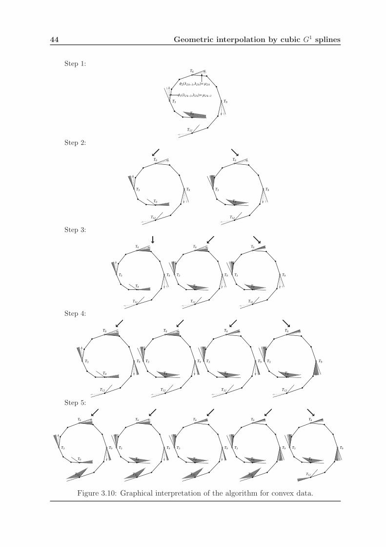
44 Geometric interpolation by cubic G1 splines
Step 1:
T0
T3
T6
T9
T12
Φ1HΛ2 k-1,Λ2 kL= Μ2 k-1
Φ2HΛ2 k-1,Λ2 kL= Μ2 k
Step 2:
ւււււււււ ցցցցցցցցց
T0
T3
T6
T9
T12
T0
T3
T6
T9
T12
Step 3:
↓↓↓↓↓↓↓↓↓ ւււււււււ ցցցցցցցցց
T0
T3
T6
T9
T12
T0
T3
T6
T9
T12
T0
T3
T6
T9
T12
Step 4:
ւււււււււ ւււււււււ ւււււււււ ցցցցցցցցց
T0
T3
T6
T9
T12
T0
T3
T6
T9
T12
T0
T3
T6
T9
T12
T0
T3
T6
T9
T12
Step 5:
ւււււււււ ւււււււււ ւււււււււ ւււււււււ ցցցցցցցցց
T0
T3
T6
T9
T12
T0
T3
T6
T9
T12
T0
T3
T6
T9
T12
T0
T3
T6
T9
T12
T0
T3
T6
T9
T12
Figure 3.10: Graphical interpretation of the algorithm for convex data.

3.4 The G1 spline curve 45
T0
T3
T6
T9
T12
T0
T3
T6
T9
T12
T0
T3
T6
T9
T12
T0
T3
T6
T9
T12
T0
T3
T6
T9
T12
Figure 3.11: All possible sets of intervals for ξℓ obtained by the algorithm.

46 Geometric interpolation by cubic G1 splines
ForwardSweep:
step 1: step 2:
T0 T3
T6
T9
T0 T3
T6
T9
step 3: step 4:
T0 T3
T6
T9
T0 T3
T6
T9
BackwardSweep:
step 5: step 6:
T0 T3
T6
T9
T0 T3
T6
T9
T0 T3
T6
T9
T0 T3
T6
T9
step 7: step 8:
T0 T3
T6
T9
T0 T3
T6
T9
T0 T3
T6
T9
T0 T3
T6
T9
Figure 3.12: Graphical interpretation of the algorithm for nonconvex data.
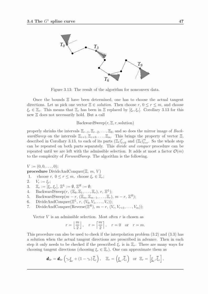
3.4 The G1 spline curve 47
T0 T3
T6
T9
Figure 3.13: The result of the algorithm for nonconvex data.
Once the bounds Ξ have been determined, one has to choose the actual tangentdirections. Let us pick one vector Ξ ∈ solution. Then choose r, 0 ≤ r ≤ m, and chooseξr ∈ Ξr. This means that Ξr has been in Ξ replaced by [ξr, ξr]. Corollary 3.13 for thisnew Ξ does not necessarily hold. But a call
BackwardSweep(r,Ξ, r, solution)
properly shrinks the intervals Ξr−1,Ξr−2, . . . ,Ξ0, and so does the mirror image of Back-wardSweep on the intervals Ξr+1,Ξr+2, . . . ,Ξm. This brings the property of vector Ξ,described in Corollary 3.13, to each of its parts (Ξℓ)
rℓ=0 and (Ξℓ)
mℓ=r. So the whole step
can be repeated on both parts separately. This divide and conquer procedure can berepeated until we are left with the admissible selection. It adds at most a factor O(m)to the complexity of ForwardSweep. The algorithm is the following.
V := (0, 0, . . . , 0);procedure DivideAndConquer(Ξ, m, V )1. choose r, 0 ≤ r ≤ m, choose ξr ∈ Ξr;2. Vr := ξr;3. Ξr := [ξr, ξr], ΞL := ∅, ΞR := ∅;4. BackwardSweep(r, (Ξ0,Ξ1, . . . ,Ξr), r, ΞL);5. BackwardSweep(m − r, (Ξm,Ξm−1, . . . ,Ξr), m− r, ΞR);6. DivideAndConquer(ΞL, r, (V0, V1, . . . , Vr));7. DivideAndConquer(Reverse(ΞR), m− r, (Vr, Vr+1, . . . , Vm));
Vector V is an admissible selection. Most often r is chosen as
r =⌊m
2
⌋
, r =⌈m
2
⌉
, r = 0 or r = m.
This procedure can also be used to check if the interpolation problem (3.2) and (3.3) hasa solution when the actual tangent directions are prescribed in advance. Then in eachstep it only needs to be checked if the prescribed ξr is in Ξr. There are many ways forchoosing tangent directions (choosing ξr ∈ Ξr). One can approximate them as
ddddddddd3r = ddddddddd3r
(
γrξr+ (1 − γr) ξr
)
, Ξr =(
ξr, ξr
)
or Ξr =[
ξr, ξr
]
,

48 Geometric interpolation by cubic G1 splines
where γr can simply be chosen as a constant or determined by some local approximationscheme from the data (3.1). Namely, interpolating polynomials with respect to certainparameterization like chord length or uniform may determine the directions in the fol-lowing way. Let pppppppppr denote the interpolating polynomial through points TTTTTTTTT 3r−j, . . . , TTTTTTTTT 3r−1,TTTTTTTTT 3r, TTTTTTTTT 3r+1, . . . , TTTTTTTTT 3r+j at some chosen parameter values
u3r−j, . . . , u3r−1, u3r, u3r+1, . . . , u3r+j.
Then γr can be determined so that ddddddddd3r is the derivative of pppppppppr at u3r. But it can happenthat γrξr
+ (1 − γr) ξr falls out of the interval Ξr. If that happens γr must be chosenin some other way, and in that case the admissible selection may depend on the r wechoose in the DivideAndConquer procedure.
Also, with the help of Ξ, one may look for a G2 spline curve with ddddddddd3ℓ determinedimplicitly as a solution of the system (3.4).
3.5. Examples
Let us conclude this chapter with some numerical examples. As the first example let thedata points be given as
TTTTTTTTT 0 = (7,−24)T , TTTTTTTTT 1 = (20,−18)T , TTTTTTTTT 2 = (24,−6)T , TTTTTTTTT 3 = (17, 4)T ,
TTTTTTTTT 4 = (4, 9)T , TTTTTTTTT 5 = (−15, 9)T , TTTTTTTTT 6 = (−23, 17)T , TTTTTTTTT 7 = (−24, 29)T ,
TTTTTTTTT 8 = (−13, 40)T , TTTTTTTTT 9 = (8, 43)T , TTTTTTTTT 10 = (24, 37)T , TTTTTTTTT 11 = (28, 28)T ,
TTTTTTTTT 12 = (38, 25)T , TTTTTTTTT 13 = (51, 29)T , TTTTTTTTT 14 = (56, 37)T , TTTTTTTTT 15 = (70, 42)T ,
TTTTTTTTT 16 = (83, 39)T , TTTTTTTTT 17 = (91, 25)T , TTTTTTTTT 18 = (88, 11)T .
Further, let the first and the last tangent direction be prescribed as
ddddddddd0 =1
2√
82(18,−2)T , ddddddddd18 =
1√218
(−13,−7)T .
Algorithm ForwardSweep returns the set solution with two admissible vectors of intervals
solution = {Ξ1,Ξ2},Ξ1 := {[0.625698, 0.625698], (0.295393, 0.893511), (0, 0.634404), (0.355009, 0.987411),
(0, 1), (0.00770851, 0.684009), [0.403509, 0.403509]}Ξ2 := {[0.625698, 0.625698], (0.295393, 0.806989), (0.634404, 1), (0, 0.355009)
(0.0656466, 1), (0.00770851, 0.684009), [0.403509, 0.403509]}.
By the DivideAndConquer procedure where r is chosen as⌊
m2
⌋and ξr as the middle
value of the interval Ξr the admissible selection reads
ξ0 = 0.625698, ξ1 = 0.594452, ξ2 = 0.317202, ξ3 = 0.67121, (3.21)
ξ4 = 0.509024, ξ5 = 0.40432, ξ6 = 0.403509,

3.5 Examples 49
for the vector Ξ1 and
ξ0 = .625698, ξ1 = 0.551191, ξ2 = 0.817202, ξ3 = 0.177505, (3.22)
ξ4 = 0.546479, ξ5 = 0.398809, ξ6 = 0.403509,
for the vector Ξ2. As described in the previous subsection the parameters ξℓ may also bedetermined by some local approximation scheme. Table 3.4 shows selections obtained byusing interpolating polynomials of degrees 2, 4, 6 based upon uniform and chord lengthparameterization. Note that all selections are admissible. The best choice would prob-
uniform parameterization chord length parameterization
degree 2 degree 4 degree 6 degree 2 degree 4 degree 6
ξ0 0.625698 0.625698 0.625698 0.625698 0.625698 0.625698ξ1 0.5 0.50634 0.480129 0.434402 0.483794 0.494794ξ2 0.5 0.527159 0.563559 0.468864 0.466898 0.468311ξ3 0.5 0.525746 0.524849 0.606469 0.531615 0.395345ξ4 0.5 0.515385 0.518351 0.370748 0.398726 0.404478ξ5 0.5 0.432277 0.414843 0.553885 0.55851 0.591284ξ6 0.403509 0.403509 0.403509 0.403509 0.403509 0.403509
Table 3.4: Admissible selections determined by interpolating polynomials based uponuniform and chord length parameterization.
ably be to compute the parameters so that the spline is not only G1 but also G2. Bysolving the system (3.4) one obtains
ξ0 = 0.625698, ξ1 = 0.496926, ξ2 = 0.539584, ξ3 = 0.448597,
ξ4 = 0.38032, ξ5 = 0.646376, ξ6 = 0.403509.
Figure 3.14 shows the comparison between the G2 spline (dashed) and G1 splines withtangent directions given by (3.21) (light gray) and (3.22) (dark gray). One can checkthat the difference between G1 splines obtained by interpolating polynomials of differentdegrees with the same parameterization (uniform or chord length) is almost impercep-tible. A comparison between G2 spline (dashed) and G1 spline with tangent directionsobtained by quadratic interpolating polynomials is shown in Figure 3.15.
For the next example let the data points be given as
TTTTTTTTT 0 = (−45,−14)T , TTTTTTTTT 1 = (−36,−11)T , TTTTTTTTT 2 = (−28,−14)T ,
TTTTTTTTT 3 = (−18,−15)T , TTTTTTTTT 4 = (−9,−11)T , TTTTTTTTT 5 = (−4,−1)T ,
TTTTTTTTT 6 = (9, 3)T , TTTTTTTTT 7 = (21, 0)T , TTTTTTTTT 8 = (27,−8)T , TTTTTTTTT 9 = (37,−15)T ,
TTTTTTTTT 10 = (48,−15)T , TTTTTTTTT 11 = (63,−10)T , TTTTTTTTT 12 = (65,−1)T ,
and the first and the last tangent direction prescribed as
ddddddddd0 =1√61
(6, 5)T , ddddddddd12 =1√89
(−5, 8)T .

50 Geometric interpolation by cubic G1 splines
Figure 3.14: A comparison between G2 (dashed) and G1 spline curves with tangentdirections given by (3.21) (light gray) and (3.22) (dark gray).
Figure 3.15: A comparison between G2 (dashed) and G1 (gray) spline curves with tangentdirections obtained by quadratic interpolating polynomials based upon uniform (left) andchord length (right) parameterization.
Algorithm ForwardSweep now returns the set with one admissible vector of intervals
Ξ := {[0.682353, 0.682353], (0.187934, 0.976309), (0, 1),
(0.11408, 0.908464), [0.296117, 0.296117]}.
By DivideAndConquer procedure with r chosen as⌊
m2
⌋and ξr as the middle value of the
interval Ξr the admissible selection reads
ξ0 = 0.682353, ξ1 = 0.534038, ξ2 = 0.5, ξ3 = 0.541808, ξ4 = 0.296117. (3.23)
Selections obtained by using interpolating polynomials of degrees 2, 4, 6 based upon uni-form and chord length parameterization are shown in Table 3.5. Again all the selectionsare admissible. By choosing
ξ0 = 0.682353, ξ1 = 0.410077, ξ2 = 0.61075, ξ3 = 0.74838, ξ4 = 0.296117,
one obtains a G2 spline. Figure 3.16 shows the comparison between G2 spline (dashed)and G1 spline (gray) with tangent directions given by (3.23). A comparison between G2

3.5 Examples 51
uniform parameterization chord length parameterization
degree 2 degree 4 degree 6 degree 2 degree 4 degree 6ξ0 0.682353 0.682353 0.682353 0.682353 0.682353 0.682353ξ1 0.5 0.423453 0.391853 0.510101 0.463167 0.468158ξ2 0.5 0.51706 0.533981 0.547337 0.544507 0.557311ξ3 0.5 0.454741, 0.451198 0.551852 0.542437 0.57377ξ4 0.296117 0.296117 0.296117 0.296117 0.296117 0.296117
Table 3.5: Admissible selections determined by interpolating polynomials based uponuniform and chord length parameterization.
Figure 3.16: A comparison between G2 (dashed) and G1 (gray) spline curves with tangentdirections given by (3.23).
spline (dashed) andG1 spline with tangent directions obtained by quadratic interpolatingpolynomials is shown in Figure 3.17.
For the last example the data points are chosen as
TTTTTTTTT 0 = (−44,−12)T , TTTTTTTTT 1 = (−42,−4)T , TTTTTTTTT 2 = (−37, 4)T ,
TTTTTTTTT 3 = (−28, 11)T , TTTTTTTTT 4 = (−17, 10)T , TTTTTTTTT 5 = (−11, 2)T ,
TTTTTTTTT 6 = (−2,−4)T , TTTTTTTTT 7 = (7,−1)T , TTTTTTTTT 8 = (11, 7)T , TTTTTTTTT 9 = (19, 12)T ,
TTTTTTTTT 10 = (31, 10)T , TTTTTTTTT 11 = (37, 3)T , TTTTTTTTT 12 = (40,−7)T ,
and the first and the last tangent direction prescribed as
ddddddddd0 = (0, 1)T , ddddddddd12 =1√104
(2,−10)T .

52 Geometric interpolation by cubic G1 splines
Figure 3.17: A comparison between G2 (dashed) and G1 (gray) spline curves with tangentdirections obtained by quadratic interpolating polynomials based upon uniform (left) andchord length parameterization.
Algorithm ForwardSweep again returns the set with one admissible vector of intervals
Ξ := {[0.714286, 0.714286], (0.247924, 1), (0.10384, 0.9800461),
(0.463815, 1), [0.178571, 0.178571]},
and DivideAndConquer procedure gives the admissible selection
ξ0 = 0.714286, ξ1 = 0.623962, ξ2 = 0.541943, ξ3 = 0.731908, ξ4 = 0.178571.(3.24)
Admissible selections obtained by interpolating polynomials of degrees 2, 4, 6 based upon
degree 2 degree 4 degree 6ξ0 0.714286 0.714286 0.714286ξ1 0.5 0.47043 0.456363ξ2 0.5 0.485632 0.489807ξ3 0.5 0.494949 0.509434ξ4 0.178571 0.178571 0.178571
Table 3.6: Admissible selections determined by interpolating polynomials based uponuniform parameterization.
uniform parameterization are given in Table 3.6. But interpolating polynomials based onchord length parameterization do not give admissible tangent directions. Furthermore, aG2 spline curve can not be found. A comparison between theG1 spline curve with tangent

3.5 Examples 53
directions given by (3.24) and the G1 spline curve with tangent directions obtained byquadratic interpolating polynomials based upon uniform parameterization is shown inFigure 3.18.
Figure 3.18: The G1 spline curve with tangent directions given by (3.24) (black) and theG1 spline curve with tangent directions obtained by quadratic interpolating polynomialsbased upon uniform parameterization (gray).


Chapter 4
Hermite geometric interpolation bycubic G1 splines
In this chapter Hermite geometric interpolation by planar cubic G1 splines is studied.Three data points and three tangent directions are interpolated per each polynomialsegment. Sufficient conditions for the existence of such G1 spline are determined thatcover most of the cases encountered in practical applications. The existence requirementsare based only upon geometric properties of data and can easily be verified in advance.The optimal approximation order six is confirmed, too.
4.1. Interpolation problem
The problem considered is the following. Suppose that 2m + 1 points and tangentdirections
TTTTTTTTT i ∈ R2, dddddddddi ∈ R
2, TTTTTTTTT i 6= TTTTTTTTT i+1, ‖dddddddddi‖2 = 1, i = 0, 1, . . . , 2m,
are given. Find a cubic G1 spline curve SSSSSSSSS : [0, 1] → R2 with prescribed breakpoints(t2i)
mi=0,
0 =: t0 < t1 < · · · < t2m−1 < t2m := 1,
that interpolates the data points TTTTTTTTT i and tangent directions dddddddddi at parameters ti,
SSSSSSSSS(ti) = TTTTTTTTT i,1
‖SSSSSSSSS′(ti)‖2SSSSSSSSS ′(ti) = dddddddddi, i = 0, 1, . . . , 2m, (4.1)
where (t2i−1)mi=1 are the unknowns. Note that (4.1) makes sense even if SSSSSSSSS ′ jumps at
the breakpoint t2i since the tangent direction is continuous. This interpolation schemeis quite clearly local. Namely, the change of one point or one tangent direction affectsonly those segments that the point or the direction belongs to. So all the analysis andestimations can be done locally.

56 Hermite geometric interpolation by cubic G1 splines
For a motivation, let us consider some numerical examples. First, suppose that thedata are sampled from an exponential and logarithmic spiral
fffffffff1(t) := exp
(t
4
)(cos tsin t
)
, t ∈ [0, 3π], fffffffff2(t) := log (1 + t)
(cos tsin t
)
, t ∈ [0, 4π],
at equidistantly chosen parameters in the parameter domain. In Figure 4.1 interpolatingG1 spline curves composed of five segments, i.e., m = 5, are shown for each curve fffffffff 1 andfffffffff 2. The parametric error estimates between fffffffff 1, fffffffff2 and their interpolants are
dist (SSSSSSSSS, fffffffff1) = 0.007915, dist (SSSSSSSSS, fffffffff 2) = 0.051094.
Considering a single segment case, Table 4.1 numerically suggests that the approxima-
T0
T1T2
T2 m-2T2 m-1
T2 m
d0
d1d2
d2 m-2d2 m-1
d2 m
T0
T1T2
T2 m-2
T2 m-1
T2 m
d0
d1
d2
d2 m-2
d2 m-1
d2 m
Figure 4.1: The interpolating G1 spline curves SSSSSSSSS for data obtained from curves fffffffff 1 (left)and fffffffff 2 (right).
tion order, measured in the parametric distance, is optimal, i.e., 6. However, the data
T0
T1
T2
T2 m-2
T2 m-1
T2 md0
d1
d2
d2 m-2
d2 m-1
d2 m
T0
T1
T2T2 m-2
T2 m-1
T2 m
d0
d1
d2 d2 m-2
d2 m-1
d2 m
Figure 4.2: Cubic G1 spline curves SSSSSSSSS for given data points and tangent directions.
do not need to be sampled from smooth curves only, they can be provided in some otherway, maybe given by the user for design purposes, obtained from some other application,etc. The data do not need to be convex either. Figure 4.2 shows some more examples

4.1 Interpolation problem 57
Interval Approximation error Decay exponentfffffffff 1 fffffffff 2 fffffffff1 fffffffff 2
[0, π] 3.3754 × 10⁻² 2.2251 × 10⁻¹ / /[0, 9π
10
]1.6644 × 10⁻² 1.0817 × 10⁻¹ 6.71 6.85
[0, 8π
10
]7.6630 × 10⁻³ 5.1067 × 10⁻² 6.59 6.37
[0, 7π
10
]3.2233 × 10⁻³ 2.2485 × 10⁻² 6.49 6.14
[0, 6π
10
]1.2017 × 10⁻³ 8.8151 × 10⁻³ 6.40 6.07
[0, 5π
10
]3.7917 × 10⁻⁴ 2.8939 × 10⁻³ 6.33 6.11
[0, 4π
10
]9.3807 × 10⁻⁵ 7.2252 × 10⁻⁴ 6.26 6.22
[0, 3π
10
]1.5773 × 10⁻⁵ 1.4194 × 10⁻⁴ 6.20 6.39
Table 4.1: The errors between curves fffffffff 1 and fffffffff2 and their polynomial geometric inter-polants.
and, as one can see, the spline follows the shape of the data quite nicely.
The next two theorems give the main results of this chapter.
THEOREM 4.1. Suppose that 2m+ 1 points and tangent directions
TTTTTTTTT i ∈ R2, dddddddddi ∈ R
2, TTTTTTTTT i 6= TTTTTTTTT i+1, ‖dddddddddi‖2 = 1, i = 0, 1, . . . , 2m,
are given. If on each segment [t2ℓ−2, t2ℓ], ℓ = 1, 2, . . . , m, one of the sufficient conditionsprescribed by Theorem 4.10, 4.11, 4.13 or 4.15 is fulfilled, then a cubic G1 spline curveSSSSSSSSS that satisfies (4.1) exists.
THEOREM 4.2. Suppose that the data are sampled from a smooth convex regularparametric curve fffffffff : [a, b] → R2 at parameter values si, a = s0 < s1 < · · · < s2m = b,
TTTTTTTTT i = fffffffff(si), dddddddddi =1
‖fffffffff ′(si)‖2
fffffffff ′(si), i = 0, 1, . . . , 2m,
and let h := max{∆si : i = 1, 2, . . . , 2m− 1}. Then one can find constants h0 > 0 andC > 0 such that for all h, 0 < h ≤ h0, a cubic G1 spline curve SSSSSSSSS that satisfies (4.1) exists,and approximates fffffffff with the optimal approximation order six, i.e., dist(fffffffff, SSSSSSSSS) ≤ C h6.
The outline of this chapter is as follows. In Subsection 4.2 a system of equationsis derived for a single segment case. The next subsection provides the conditions thatimply the solution to attain the values that are not allowed. These results togetherwith the number of solutions for some particular data lead to the existence theoremsof Subsection 4.4. They are proved in Subsection 4.5 by the help of convex homotopyand Brouwer’s degree argument. The last subsection deals with asymptotic analysis andcontains the proof of Theorem 4.2.

58 Hermite geometric interpolation by cubic G1 splines
4.2. Single segment case
Since the G1 interpolation scheme (4.1) is local, all the properties can be determinedfrom the simplest case m = 1. So from now on to the end of this chapter we assumem = 1. For m = 1 let the spline SSSSSSSSS be denoted by PPPPPPPPP . The equations (4.1) simplify to
PPPPPPPPP (ti) = TTTTTTTTT i, PPPPPPPPP ′(ti) = αidddddddddi, αi > 0, i = 0, 1, 2, (4.2)
with 0 := t0 < t1 < t2 := 1. One is thus left with twelve equations for eight unknowncoefficients of PPPPPPPPP , and four unknown parameters t1, α0, α1, and α2.
REMARK 4.3. If the tangent directions are not normalized that does not effect theexistence of the solution of (4.2). Only the magnitudes of αi, i = 0, 1, 2, change.
The first step is to separate the unknown coefficients from the rest of the unknowns.For any t1, α0, α1 and α2 there exists a unique polynomial ppppppppp5 of degree ≤ 5 that solvesthe interpolation problem (4.2). But this ppppppppp5 will be of degree three, i.e., ppppppppp5 = PPPPPPPPP , iff thecoefficients at powers 4 and 5 are zero. This is true iff
[t0, t0, t1, t1, t2]ppppppppp5 = 0, [t0, t1, t1, t2, t2]ppppppppp5 = 0, (4.3)
which gives the system of four equations for four unknowns t1, α0, α1, α2, that must liein an open set
U := {t1; 0 < t1 < 1} × {(α0, α1, α2); αi > 0, i = 0, 1, 2}.
Establishing these parameters is the only nonlinear part of the problem. The coefficientsof PPPPPPPPP are then obtained by using any standard interpolation scheme componentwise.Since t0 = 0 and t2 = 1 the equations (4.3) simplify to
α0
t21ddddddddd0 +
α1
(1 − t1) t21
ddddddddd1 −(2 + t1)
t31∆TTTTTTTTT 0 −
1
(1 − t1)2 ∆TTTTTTTTT 1 = 0, (4.4)
α1
(1 − t1)2 t1
ddddddddd1 +α2
(1 − t1)2ddddddddd2 −
1
t21∆TTTTTTTTT 0 +
(t1 − 3)
(1 − t1)3 ∆TTTTTTTTT 1 = 0.
To simplify the analysis it will be assumed from now on that the points TTTTTTTTT 0, TTTTTTTTT 1 and TTTTTTTTT 2
are not collinear. Using det (·,∆TTTTTTTTT 0) and det (·,∆TTTTTTTTT 1) on (4.4) one obtains
α0
t21det (ddddddddd0,∆TTTTTTTTT 0) −
α1
(1 − t1) t21
det (∆TTTTTTTTT 0, ddddddddd1) +1
(1 − t1)2 det (∆TTTTTTTTT 0,∆TTTTTTTTT 1) = 0,
α0
t21det (ddddddddd0,∆TTTTTTTTT 1) +
α1
(1 − t1) t21det (ddddddddd1,∆TTTTTTTTT 1) −
(2 + t1)
t31det (∆TTTTTTTTT 0,∆TTTTTTTTT 1) = 0,
(4.5)
α1
(1 − t1)2 t1
det (∆TTTTTTTTT 0, ddddddddd1) +α2
(1 − t1)2 det (∆TTTTTTTTT 0, ddddddddd2) +
(t1 − 3)
(1 − t1)3 det (∆TTTTTTTTT 0,∆TTTTTTTTT 1) = 0,
α1
(1 − t1)2 t1
det (ddddddddd1,∆TTTTTTTTT 1) −α2
(1 − t1)2 det (∆TTTTTTTTT 1, ddddddddd2) −
1
t21det (∆TTTTTTTTT 0,∆TTTTTTTTT 1) = 0.

4.2 Single segment case 59
Let us define the constants that are determined by the data as
λ1 :=det (ddddddddd0,∆TTTTTTTTT 0)
det (∆TTTTTTTTT 0,∆TTTTTTTTT 1), λ2 :=
det (∆TTTTTTTTT 0, ddddddddd1)
det (∆TTTTTTTTT 0,∆TTTTTTTTT 1),
λ3 :=det (ddddddddd1,∆TTTTTTTTT 1)
det (∆TTTTTTTTT 0,∆TTTTTTTTT 1), λ4 :=
det (∆TTTTTTTTT 1, ddddddddd2)
det (∆TTTTTTTTT 0,∆TTTTTTTTT 1), (4.6)
µ1 :=det (ddddddddd0,∆TTTTTTTTT 1)
det (∆TTTTTTTTT 0,∆TTTTTTTTT 1), µ2 :=
det (∆TTTTTTTTT 0, ddddddddd2)
det (∆TTTTTTTTT 0,∆TTTTTTTTT 1).
Their signs have a nice geometric interpretation as one can see in Figure 4.3. Noteagain that the definition of the constants λi and µi differs from that in Chapter 2 andChapter 3. With these constants, the equations (4.5) become
Λ1>0Μ1< 0
Λ1>0Μ1< 0
Λ1< 0Μ1>0
Λ1< 0Μ1< 0
Λ2>0Λ3>0
Λ2>0Λ3< 0
Λ2< 0Λ3< 0
Λ2< 0Λ3>0
Λ4< 0Μ2>0
Λ4>0Μ2>0
Λ4>0Μ2< 0
Λ4< 0Μ2< 0
DT0 DT1
Figure 4.3: Geometric interpretation of signs of the constants λi and µi.
FFFFFFFFF (t1, ααααααααα) := FFFFFFFFF (t1, ααααααααα;λλλλλλλλλ, µ1, µ2) := (Fi(t1, ααααααααα))4i=1 = 000000000,
where
F1(t1, ααααααααα) := λ1α0
t21− λ2
α1
t21 (1 − t1)+
1
(1 − t1)2 = 0,
F2(t1, ααααααααα) := µ1α0
t21+ λ3
α1
t21 (1 − t1)− (2 + t1)
t31= 0, (4.7)
F3(t1, ααααααααα) := µ2α2
(1 − t1)2 + λ2
α1
(1 − t1)2 t1
− (3 − t1)
(1 − t1)3 = 0,
F4(t1, ααααααααα) := λ4α2
(1 − t1)2 − λ3
α1
(1 − t1)2 t1
+1
t21= 0.
Here ααααααααα := (αi)2i=0, λλλλλλλλλ := (λi)
4i=1. Moreover, if
λ1λ3 + λ2µ1 6= 0, λ2λ4 + λ3µ2 6= 0, (4.8)

60 Hermite geometric interpolation by cubic G1 splines
equations (4.7) can be rewritten as
α0 =(t31 − 3t1 + 2)λ2 − t31λ3
(t1 − 1)2 t1 (λ1λ3 + λ2µ1),
α1 = − µ1t31 + (t31 − 3t1 + 2)λ1
(t1 − 1) t1 (λ1λ3 + λ2µ1), (4.9)
α2 =(t1 − 3) t21λ3 − (t1 − 1)3 λ2
(t1 − 1) t21 (λ2λ4 + λ3µ2),
andµ1t
31 + (t31 − 3t1 + 2)λ1
λ1λ3 + λ2µ1+µ2 (t1 − 1)3 + (t1 − 3) t21λ4
λ2λ4 + λ3µ2= 0. (4.10)
The only nonlinear part that remains is (4.10) which is a cubic equation for t1 that caneasily be solved numerically. Since the unknowns must lie in U , the next lemma followsdirectly from equations (4.7).
LEMMA 4.4. A cubic polynomial curve PPPPPPPPP that satisfies (4.2) does not exist in any ofthe following cases:
1. λ2 ≤ 0 and λ1 ≥ 0, 2. λ3 ≤ 0 and λ4 ≥ 0,
3. λ3 ≤ 0 and µ1 ≤ 0, 4. λ2 ≤ 0 and µ2 ≤ 0.
As can be seen in Figure 4.3 cases where one of λi is equal to zero are very exceptionaland for the sake of simplicity it will be assumed from now on that λi 6= 0, i = 1, 2, 3, 4.The first step to the existence of PPPPPPPPP is to find the relations between the data that forcethe solution of (4.7) to approach the boundary ∂U . This analysis is given in the nextsubsection.
4.3. Relations, implying the solution to approach
the boundary
If the solution (t1, ααααααααα) touches the boundary ∂U , it attains the values that are not allowed.As it turns out this implies certain relations between data that could be used to avoidthe parameter choices that are not admissible. The next two lemmas reveal the relationsfor t1 → 0, 1.
LEMMA 4.5. Suppose that λi 6= 0, i = 1, 2, 3, 4. Parameter t1 tends to zero if
µ2 → ϕ2(λλλλλλλλλ, µ1) :=2λ1λ2λ4
λ2µ1 − λ1λ3,
and λ1λ2 > 0, and one of the three following conditions hold:
λ3 > 0, λ4 > 0, −λ1λ3
λ2< µ1 <
λ1λ3
λ2, or
λ3 > 0, λ4 < 0,λ1λ3
λ2< µ1, or
λ3 < 0, λ4 < 0, −λ1λ3
λ2< µ1.
4.3 Relations, implying the solution to approach the boundary 61
Under these conditions λ1ϕ2(λλλλλλλλλ, µ1) < 0.
LEMMA 4.6. Suppose that λi 6= 0, i = 1, 2, 3, 4. Parameter t1 tends to one if
µ1 → ϕ1(λλλλλλλλλ, µ2) :=2λ1λ3λ4
λ3µ2 − λ2λ4
,
and λ3λ4 > 0, and one of the three following conditions hold:
λ1 > 0, λ2 > 0, −λ2λ4
λ3< µ2 <
λ2λ4
λ3, or
λ1 < 0, λ2 > 0,λ2λ4
λ3< µ2, or
λ1 < 0, λ2 < 0, −λ2λ4
λ3< µ2.
Under these conditions λ4ϕ1(λλλλλλλλλ, µ2) < 0.
Proof. From the symmetry between λi, λ5−i, i = 1, 2, and µ1, µ2, and the symmetry inequations (4.7) it is enough to prove Lemma 4.5 only. If λ1λ3 + λ2µ1 = 0, the first twoequations in (4.7) become
α0 =−t21 + (1 − t1)α1λ2
(1 − t1)2 λ1
,λ3
(1 − t1)2 λ2
− t1 + 2
t31= 0.
Therefore it is clear that t1 cannot approach zero or one. The same is true whenλ2λ4 + λ3µ2 = 0. Thus let us assume that conditions (4.8) hold. Equation (4.10) can berewritten as
2λ1
λ1λ3 + λ2µ1− µ2
λ2λ4 + λ3µ2+ O(t1) = 0,
and t1 → 0 implies µ2 → ϕ2(λλλλλλλλλ, µ1). Moreover,
limt1→0
(t1α0) =2λ2
λ1λ3 + λ2µ1, lim
t1→0(t1α1) =
2λ1
λ1λ3 + λ2µ1,
limt1→0
(t21α2
)= − λ2
λ2λ4 + λ3µ2
.
It is now easy to check that ααααααααα is positive iff the conditions in the lemma are fulfilled,and further that λ1ϕ2(λλλλλλλλλ, µ1) < 0, which completes the proof.
The relations implied by αi = 0 are given in the next lemma.
LEMMA 4.7. Parameter α0 = 0 if λi > 0 for i = 2, 3, 4, and µ2 = ψ2(λλλλλλλλλ), where
ψ2(λλλλλλλλλ) := λ4τ(λ2, λ3)
2(3 − 2τ(λ2, λ3))
(1 − τ(λ2, λ3))2(1 + 2τ(λ2, λ3))> 0,
and τ(λ2, λ3) is defined as a unique solution t1 of the problem
g(t1;λ2, λ3) :=1
λ2
t211 − t1
− 1
λ3
(1 − t1)(2 + t1)
t1= 0, 0 < t1 < 1. (4.11)

62 Hermite geometric interpolation by cubic G1 splines
Similarly, parameter α2 = 0 if λi > 0 for i = 1, 2, 3, and µ1 = ψ1(λλλλλλλλλ), where
ψ1(λλλλλλλλλ) := λ1τ(λ3, λ2)
2(3 − 2τ(λ3, λ2))
(1 − τ(λ3, λ2))2(1 + 2τ(λ3, λ2))> 0.
Moreover, parameter α1 = 0 if λ1 < 0, λ4 < 0, µ1 > 0 and
µ2 = ψ3(λ1, λ4, µ1) := −λ4(3 − τ(−λ1, µ1)) τ(−λ1, µ1)
2
(1 − τ(−λ1, µ1))3 > 0.
Proof. First let us prove that for λ2 > 0 and λ3 > 0, the equation (4.11) has a uniquesolution. Since
limt1↓0
g(t1;λ2, λ3) = −sign
(1
λ3
)
· ∞ = −∞, limt1↑1
g(t1;λ2, λ3) = sign
(1
λ2
)
· ∞ = ∞,
(4.12)
limt1→−∞
g(t1;λ2, λ3) = sign
(1
λ2− 1
λ3
)
· ∞, limt1→∞
g(t1;λ2, λ3) = −sign
(1
λ2− 1
λ3
)
· ∞,
there exists at least one t1 ∈ (0, 1) that solves (4.11). It is straightforward to computethat when λ2 = λ3 the solution is unique, i.e., τ(λ2, λ3) := 2/3. Now, for λ2 6= λ3 theonly possible solutions are
t1 =λ2(λ3 − λ2) − σ
23
(λ3 − λ2)σ13
, (4.13)
t ±1 =(1 ± i
√3)λ2(λ3 − λ2) + (−1 ± i
√3)σ
23
2(λ2 − λ3)σ13
, (4.14)
whereσ := λ2(λ3 − λ2)
(
λ2 − λ3 +√
λ3(λ3 − λ2))
.
For λ3 > λ2 it is clear that σ is a real number, so solutions (4.14) are complex, thus(4.13) is a unique admissible solution and τ(λ2, λ3) := t1. For λ3 < λ2 the function ghas three real zeros, but it follows from (4.12) that only one of them is in (0, 1), namelyτ(λ2, λ3) := t +
1 .Let us now analyse the case α0 = 0. From the first and the third equation in (4.7)
one obtains
λ2α1 =t21
1 − t1, µ2 =
1
α2
3 − 2t1(1 − t1)
, (4.15)
and from the remaining equations
λ3α1 =(1 − t1)(2 + t1)
t1, λ4α2 =
(1 − t1)(1 + 2t1)
t21. (4.16)
Therefore it follows that the system (4.15)–(4.16) has an admissible solution α1 > 0,α2 > 0 and t1 ∈ (0, 1) iff λ2 > 0, λ3 > 0, λ4 > 0 and µ2 = ψ2(λλλλλλλλλ). The proof for the caseα2 = 0 is symmetric to this one and it will be omitted.

4.3 Relations, implying the solution to approach the boundary 63
Suppose now that α1 = 0. It is clear from (4.7) that neither λ1 nor λ4 can be equalto zero. From the first and the last equation in (4.7) one obtains
α0 = − t21(t1 − 1)2 λ1
, α2 = −(t1 − 1)2
t21λ4.
The remaining two equations then simplify to
−t1 + 2
t31− µ1
(t1 − 1)2 λ1
= 0,3 − t1
(t1 − 1)3− µ2
t21λ4= 0. (4.17)
Since the solution must be in U , it is clear that λ1 < 0, λ4 < 0, µ1 > 0 and µ2 >
0. Multiplying the first equation in (4.17) by1
µ1t21(1 − t1) the equation rewrites to
g(t1;−λ1, µ1) = 0. Since −λ1 > 0 and µ1 > 0 there exists a unique τ(−λ1, µ1) ∈ (0, 1)that solves it. From (4.17) it then follows that
µ1 > 0, µ2 = ψ3(λ1, λ4, µ1), or equivalently µ2 > 0, µ1 = ψ4(λ1, λ4, µ2),
where ψ4(λ1, λ4, µ) := ψ3(λ4, λ1, µ). This completes the proof.
The following properties of functions ϕi and ψi will be needed.
LEMMA 4.8. If λλλλλλλλλ > 0 then
− λ1λ3
λ2
< µ1 <λ1λ3
λ2
=⇒ ϕ2(λλλλλλλλλ, µ1) < −λ2λ4
λ3
, (4.18)
− λ2λ4
λ3
< µ2 <λ2λ4
λ3
=⇒ ϕ1(λλλλλλλλλ, µ2) < −λ1λ3
λ2
. (4.19)
Also, if λλλλλλλλλ < 0, then
µ1 > −λ1λ3
λ2=⇒ ϕ2(λλλλλλλλλ, µ1) < −λ2λ4
λ3, (4.20)
µ2 > −λ2λ4
λ3=⇒ ϕ1(λλλλλλλλλ, µ2) < −λ1λ3
λ2. (4.21)
Furthermore, for λ1 > 0, λ2 > 0, λ3 < 0 and λ4 < 0 the following implication holds:
µ1 > −λ1λ3
λ2
=⇒ −λ2λ4
λ3
< ϕ2(λλλλλλλλλ, µ1) <λ2λ4
λ3
+2λ1λ4
µ1
<λ2λ4
λ3
. (4.22)
LEMMA 4.9. For λλλλλλλλλ > 0 functions ψi are bounded from below as
λ1λ3
λ2< ψ1(λλλλλλλλλ) and
λ2λ4
λ3< ψ2(λλλλλλλλλ). (4.23)
Moreover, for λλλλλλλλλ < 0
ϕ2(λλλλλλλλλ) < ψ3(λ1, λ4, µ1) and ϕ1(λλλλλλλλλ) < ψ4(λ1, λ4, µ2), (4.24)
2λ1λ3λ4 + λ2λ4µ1
λ3µ1< ψ3(λ1, λ4, µ1), (4.25)
and µ1 > 0, µ2 >2λ1λ3λ4 + λ2λ4µ1
λ3µ1=⇒ ϕ1(λλλλλλλλλ) < µ1. (4.26)
The proofs of Lemma 4.8 and Lemma 4.9 are elementary, but very technical. Theycan easily be done by using a Computer Algebra system’s symbolic facilities, thus theywill be omitted.

64 Hermite geometric interpolation by cubic G1 splines
4.4. Main theorems
In this subsection sufficient conditions that imply the existence of a cubic geometricinterpolant PPPPPPPPP that satisfies (4.2) will be given. There are sixteen possibilities for thesigns of λi as shown in Table 4.2. Lemma 4.4 shows that for the last seven optionsa solution of (4.7) does not exist. Other possibilities are considered in the followingtheorems.
sign(λ1) +++++++++ +++++++++ −−−−−−−−− +++++++++ −−−−−−−−− −−−−−−−−− −−−−−−−−− −−−−−−−−− −−−−−−−−− +++++++++ +++++++++ +++++++++ +++++++++ −−−−−−−−− +++++++++ −−−−−−−−−sign(λ2) +++++++++ +++++++++ +++++++++ +++++++++ −−−−−−−−− +++++++++ +++++++++ −−−−−−−−− −−−−−−−−− +++++++++ −−−−−−−−− −−−−−−−−− −−−−−−−−− +++++++++ −−−−−−−−− −−−−−−−−−sign(λ3) +++++++++ +++++++++ +++++++++ −−−−−−−−− +++++++++ +++++++++ −−−−−−−−− +++++++++ −−−−−−−−− −−−−−−−−− +++++++++ −−−−−−−−− +++++++++ −−−−−−−−− −−−−−−−−− −−−−−−−−−sign(λ4) +++++++++ −−−−−−−−− +++++++++ −−−−−−−−− +++++++++ −−−−−−−−− −−−−−−−−− −−−−−−−−− −−−−−−−−− +++++++++ +++++++++ +++++++++ −−−−−−−−− +++++++++ −−−−−−−−− +++++++++
Table 4.2: Sixteen possibilities for the signs of λi.
THEOREM 4.10. Suppose that the data TTTTTTTTT i, dddddddddi, i = 0, 1, 2, satisfy det (∆TTTTTTTTT 0,∆TTTTTTTTT 1) 6= 0and λλλλλλλλλ > 0. If one of the listed cases
1. µ1 > ψ1(λλλλλλλλλ) and µ2 > ψ2(λλλλλλλλλ),
2. λ1λ3
λ2≤ µ1 < ψ1(λλλλλλλλλ) and µ2 < ψ2(λλλλλλλλλ),
3. λ2λ4
λ3≤ µ2 < ψ2(λλλλλλλλλ) and µ1 < ψ1(λλλλλλλλλ),
4. −λ1λ3
λ2< µ1 <
λ1λ3
λ2and ϕ2(λλλλλλλλλ, µ1) < µ2 < ψ2(λλλλλλλλλ),
5. −λ2λ4
λ3< µ2 <
λ2λ4
λ3and ϕ1(λλλλλλλλλ, µ2) < µ1 < ψ1(λλλλλλλλλ),
holds, then the cubic interpolating curve PPPPPPPPP that satisfies (4.2) exists.
THEOREM 4.11. Suppose that the data TTTTTTTTT i, dddddddddi, i = 0, 1, 2, satisfy det (∆TTTTTTTTT 0,∆TTTTTTTTT 1) 6= 0,λi > 0, i = 1, 2, 3, and λ4 < 0. If
µ1 > ψ1(λλλλλλλλλ) and µ2 > ϕ2(λλλλλλλλλ, µ1), or
λ1λ3
λ2< µ1 < ψ1(λλλλλλλλλ) and µ2 < ϕ2(λλλλλλλλλ, µ1),
then the cubic interpolating curve PPPPPPPPP that satisfies (4.2) exists.
REMARK 4.12. The case λ1 < 0 and λi > 0, i = 2, 3, 4, is symmetric to the oneconsidered in Theorem 4.11. The result is the following. If
µ2 > ψ2(λλλλλλλλλ) and µ1 > ϕ1(λλλλλλλλλ, µ2), or
λ2λ4
λ3< µ2 < ψ2(λλλλλλλλλ) and µ1 < ϕ1(λλλλλλλλλ, µ2),
then the cubic interpolating curve PPPPPPPPP that satisfies (4.2) exists.

4.4 Main theorems 65
THEOREM 4.13. Suppose that the data TTTTTTTTT i, dddddddddi, i = 0, 1, 2, satisfy det (∆TTTTTTTTT 0,∆TTTTTTTTT 1) 6= 0and λ1 > 0, λ2 > 0, λ3 < 0, λ4 < 0. If
−λ1λ3
λ2< µ1 and ϕ2(λλλλλλλλλ, µ1) < µ2 <
λ2λ4
λ3+
2λ1λ4
µ1,
then the cubic interpolating curve PPPPPPPPP that satisfies (4.2) exists.
REMARK 4.14. The case where λ1 < 0, λ2 < 0, λ3 > 0, λ4 > 0 is symmetric to theone considered in Theorem 4.13, and the result is the following. If
−λ2λ4
λ3< µ2 and ϕ1(λλλλλλλλλ, µ2) < µ1 <
λ1λ3
λ2+
2λ1λ4
µ2,
then the cubic interpolating curve PPPPPPPPP that satisfies (4.2) exists.
THEOREM 4.15. Suppose that the data TTTTTTTTT i, dddddddddi, i = 0, 1, 2, satisfy det (∆TTTTTTTTT 0,∆TTTTTTTTT 1) 6= 0and λ1 < 0, λ4 < 0, µ1 > 0. If one of the following cases holds,
1. λ2 > 0, λ3 > 0, µ2 > ψ3(λ1, λ4, µ1),
2. λ2 < 0, λ3 > 0, 0 < µ1 ≤ λ1λ3
λ2, µ2 > ψ3(λ1, λ4, µ1),
3. λ2 > 0, λ3 < 0, 0 < µ2 ≤ λ2λ4
λ3, µ1 > ψ4(λ1, λ4, µ2),
4. λ2 < 0, λ3 < 0, µ1 > −λ1λ3
λ2, ϕ2(λλλλλλλλλ, µ1) < µ2 < ψ3(λ1, λ4, µ1),
5. λ2 < 0, λ3 < 0, 0 < µ1 ≤ −λ1λ3
λ2, 2λ1λ3λ4+λ2λ4µ1
λ3µ1< µ2 < ψ3(λ1, λ4, µ1),
then the cubic interpolating curve PPPPPPPPP that satisfies (4.2) exists.
REMARK 4.16. The constants λλλλλλλλλ, µ1 and µ2 change if lengths of dddddddddi change, but allthe relations in Theorems 4.10–4.15 remain the same.
These theorems provide us with sufficient conditions that imply the existence of theinterpolating polynomial. If none of these conditions is fulfilled the number of solutionsis even, in most cases zero. Let us take for example Theorem 4.10 and choose data sothat λi = 1, i = 1, 2, 3, 4, and (µ1, µ2) = (3, 1), (2, 3), (0,±3), (±3, 0), (−3,±3). In allof these examples the data do not satisfy any of the conditions of Theorem 4.10, andsince the solutions can be computed analytically, one can easily check that there is nosolution in U .
Proofs of these theorems will be made in two steps and will be given as the nextsubsection. First the existence of the solution will be proved for the particular data. Inthe second step conclusions will be carried from the particular case to a general one bya homotopy and Brouwer’s degree argument.

66 Hermite geometric interpolation by cubic G1 splines
4.5. Proofs of main theorems
Step 1: Particular cases
Let the points be chosen as
TTTTTTTTT 0 = (−1,−1)T , TTTTTTTTT 1 = (0, 0)T , TTTTTTTTT 2 = (1,−1)T , (4.27)
and the tangent directions given in Table 4.3. Tables 4.4 and 4.5 show the constants forthis data, and Table 4.6 gives the admissible solutions (t1, ααααααααα) ∈ U . Note that there is aunique admissible solution in all the cases (Figure 4.4).
ddddddddd0 ddddddddd1 ddddddddd2
data 1 (3, 5)T (2, 0)T (3,−5)T
data 2 (1, 3)T (2, 0)T (1,−3)T
data 3 (−0.5, 1.5)T (2, 0)T (−0.5,−1.5)T
data 4 (3, 5)T (2, 0)T (5,−3)T
data 5 (1, 3)T (2, 0)T (−7, 9)T
data 6 (2, 4)T (0,−2)T (1, 1)T
data 7 (7, 5)T (2, 0)T (7,−5)T
data 8 (1.8,−0.2)T (0, 2)T (41,−39)T
data 9 (3, 1)T (−2, 0)T (3,−1)T
data 10 (1.5,−0.5)T (−2, 0)T (11,−9)T
Table 4.3: The tangent directions for different choices of data.
data λ1 λ2 λ3 λ4 µ1 µ2
1 1 1 1 1 4 42 1 1 1 1 2 23 1 1 1 1 1
212
4 1 1 1 −1 4 45 1 1 1 −1 2 −86 1 1 −1 −1 3 07 −1 1 1 −1 6 68 −1 −1 1 −1 0.8 409 −1 −1 −1 −1 2 210 −1 −1 −1 −1 0.5 10
Table 4.4: The constants for the particular data.
Step 2: Homotopy
In order to prove Theorems 4.10, 4.11, 4.13 and 4.15 one must show that the system(4.7) has a solution (t1, ααααααααα) ∈ U . The conclusions for the particular data outlined in

4.5 Proofs of main theorems 67
data ψ1(λλλλλλλλλ) ψ2(λλλλλλλλλ) ϕ1(λλλλλλλλλ, µ2) ϕ2(λλλλλλλλλ, µ1) ψ3(λλλλλλλλλ, µ1)1 2.8571 2.8571 / / /2 2.8571 2.8571 / / /3 2.8571 2.8571 −4 −4 /4 2.8571 / / −2
3/
5 2.8571 / / −2 /6 / / 2 −1
2/
7 / / / / 4.17248 / / / / 36.21529 / / 2
323
12.9610 / / 2
11/ 63.1769
Table 4.5: The constants for the particular data.
data t1 α0 α1 α2
1 12
45
910
45
2 12
43
76
43
3 12
83
116
83
4 0.3624 1.2392 0.9961 0.34705 0.1902 3.8203 3.1384 1.62906 0.4462 3.0658 2.0574 6.15217 0.5 0.8 0.1 0.88 0.6860 4.8270 0.0169 0.18499 0.5 4 1.5 410 0.7620 13.2434 0.7134 1.0338
Table 4.6: The admissible solutions for the particular data.
Table 4.5 will be carried to the general case by the use of the homotopy and Brouwer’sdegree argument. Let the general data be denoted by (λλλλλλλλλ, µ1, µ2) and the particular oneby (λλλλλλλλλ∗, µ∗
1, µ∗2). A homotopy is defined as
HHHHHHHHH(t1, ααααααααα; ζ) := FFFFFFFFF (t1, ααααααααα;λλλλλλλλλ(ζ), µ1(ζ), µ2(ζ)) ,
whereλλλλλλλλλ(ζ) := (1 − ζ)λλλλλλλλλ∗ + ζλλλλλλλλλ, µi(ζ) := qi(ζ ;µ
∗i , µi), i = 1, 2,
and qi := qi(.;µ∗i , µi) : [0, 1] → R will be chosen later on as continuous piecewise linear
functions that satisfy qi(0;µ∗i , µi) = µ∗
i , qi(1;µ∗i , µi) = µi. The idea of the proof is to
connect particular and general data so that a set of solutions
V := {(t1(ζ), ααααααααα(ζ)) ∈ U ; HHHHHHHHH(t1(ζ), ααααααααα(ζ); ζ) = 000000000, ζ ∈ [0, 1]}
stays away from the boundary ∂U . If this can be done, one can find a compact setK ⊂ U , such that
V ⊂ K ⊂ U , V ∩ ∂K = ∅. (4.28)

68 Hermite geometric interpolation by cubic G1 splines
Therefore the map HHHHHHHHH does not vanish at the boundary ∂K, and Brouwer’s degree ofHHHHHHHHH onK is invariant for all ζ ∈ [0, 1]. But since it is odd for the particular map FFFFFFFFF (·, ·;λλλλλλλλλ∗, µ∗
1, µ∗2),
equations FFFFFFFFF (t1, ααααααααα;λλλλλλλλλ, µ1, µ2) = 000000000 must have at least one admissible solution.One is now left to show how to choose q1 and q2, and to prove that (4.28) holds.
Namely, it must be shown that solutions of HHHHHHHHH(t1(ζ), ααααααααα(ζ); ζ) = 000000000 satisfy
t1(ζ) ≥ const > 0, 1 − t1(ζ) ≥ const > 0, αi(ζ) ≥ const > 0, i = 0, 1, 2, (4.29)
for all ζ ∈ [0, 1]. The inequality
|λi(ζ)| ≥ minζ∈[0,1]
{|(1 − ζ)λ∗i + ζλi|} ≥ min {|λ∗i |, |λi|} ≥ const > 0
will be fulfilled, and the results of Lemma 4.5, Lemma 4.6 and Lemma 4.7 will be themain tool in the proof of all four theorems. Each of them will be analysed separately.
Theorem 4.10: There are five cases to be considered. Choosing data 1, 2 or 3 asparticular data yields λλλλλλλλλ(ζ) > 0, and thus α1(ζ) cannot approach zero, i.e., α1(ζ) ≥const > 0 for all ζ ∈ [0, 1]. In the first case where µi > ψi(λλλλλλλλλ), i = 1, 2, choose data 1 asthe particular data. Since µ∗
i > ψi(λλλλλλλλλ∗) and ψi does not depend on µi, there obviously
exists qi, such thatµi(ζ) > ψi(λλλλλλλλλ(ζ)), ζ ∈ [0, 1], i = 1, 2.
Therefore α0(ζ) and α2(ζ) cannot approach zero for any ζ ∈ [0, 1], and by (4.23) theparameter t1(ζ) cannot approach zero or one either.
Suppose now thatλ1λ3
λ2
≤ µ1 < ψ1(λλλλλλλλλ) and µ2 < ψ2(λλλλλλλλλ) (case 2) and choose data 2. There
clearly exists q2 that satisfies µ2(ζ) < ψ2(λλλλλλλλλ(ζ)) for every ζ ∈ [0, 1]. Moreover, from (4.23)
it follows thatλ1(ζ)λ3(ζ)
λ2(ζ)< ψ1(λλλλλλλλλ(ζ)), so one can find q1 such that
λ1(ζ)λ3(ζ)
λ2(ζ)< µ1(ζ) < ψ1(λλλλλλλλλ(ζ)), ζ ∈ [0, 1].
Now, it is clear that α0(ζ), α2(ζ), t1(ζ) ≥ const > 0 for all ζ ∈ [0, 1]. Moreover, by (4.19)the parameter t1(ζ) cannot approach 1 either which completes the proof. The case 3 issymmetric to the second one and will be omitted.Consider now the case 4 and choose data 3 that satisfy
−λ∗1λ
∗3
λ∗2< µ∗
1 <λ∗1λ
∗3
λ∗2and ϕ2(λλλλλλλλλ
∗, µ∗1) < µ∗
2 < ψ2(λλλλλλλλλ∗).
There obviously exists q1 such that
−λ1(ζ)λ3(ζ)
λ2(ζ)< µ1(ζ) <
λ1(ζ)λ3(ζ)
λ2(ζ), ζ ∈ [0, 1].
Since by (4.18) and (4.23)
ϕ2(λλλλλλλλλ(ζ), µ1(ζ)) < −λ2(ζ)λ4(ζ)
λ3(ζ)<λ2(ζ)λ4(ζ)
λ3(ζ)< ψ2(λλλλλλλλλ(ζ)), ζ ∈ [0, 1],

4.5 Proofs of main theorems 69
there exists q2 that satisfies ϕ2(λλλλλλλλλ(ζ), µ1(ζ)) < µ2(ζ) < ψ2(λλλλλλλλλ(ζ)). Thus α0(ζ), t1(ζ) ≥const > 0. Further, by (4.19) and (4.23), α2(ζ), 1− t1(ζ) ≥ const > 0, and (4.29) holds.The case 5 is symmetric to the case 4 and will be omitted. This completes the proof ofTheorem 4.10.
Theorem 4.11: Particular data must be chosen so that λi(ζ) > 0, i = 1, 2, 3, andλ4(ζ) < 0. It is then clear that there exists a constant ’const’ such that αi(ζ) ≥ const > 0,i = 0, 1, and 1 − t1(ζ) ≥ const > 0, no matter how we define q1 and q2. By (4.23),λ1(ζ)λ3(ζ)
λ2(ζ)< ψ1(λλλλλλλλλ(ζ)). Now, for the first case choose data 4, define q1 so that µ1(ζ) >
ψ1(λλλλλλλλλ(ζ)), and then choose such q2 that µ2(ζ) > ϕ2(λλλλλλλλλ(ζ), µ1(ζ)), ζ ∈ [0, 1]. In the secondcase choose data 5, define q1 so that
λ1(ζ)λ3(ζ)
λ2(ζ)< µ1(ζ) < ψ1(λλλλλλλλλ(ζ)), ζ ∈ [0, 1],
and choose such q2 that µ2(ζ) < ϕ2(λλλλλλλλλ(ζ), µ1(ζ)). Now, (4.29) obviously holds andTheorem 4.11 is proved.
Theorem 4.13: Let us choose data 6 as the particular data. Since λ1(ζ) > 0, λ2(ζ) > 0,λ3(ζ) < 0 and λ4(ζ) < 0 it is clear from Lemma 4.7 that αi(ζ) ≥ const > 0, i = 0, 1, 2,
for ζ ∈ [0, 1]. Let q1 be chosen in such a way that −λ1(ζ)λ3(ζ)
λ2(ζ)< µ1(ζ) for ζ ∈ [0, 1].
By using (4.22) one can find q2 that satisfies
−λ2(ζ)λ4(ζ)
λ3(ζ)< ϕ2(λλλλλλλλλ(ζ), µ1(ζ)) < µ2(ζ) <
λ2(ζ)λ4(ζ)
λ3(ζ)+
2λ1(ζ)λ4(ζ)
µ1(ζ)<λ2(ζ)λ4(ζ)
λ3(ζ).
Therefore t1(ζ) cannot approach zero for any ζ ∈ [0, 1]. Now, it can easily be provedthat µ1(ζ) > ϕ1(λλλλλλλλλ(ζ), µ1(ζ)), thus the parameter t1(ζ) cannot approach 1 either and theproof is completed.
Theorem 4.15: Particular data must be chosen so that λ1(ζ) < 0 and λ4(ζ) < 0. Thenit is clear that αi(ζ) ≥ const > 0, i = 0, 2, for all ζ ∈ [0, 1]. In the case 1 choosedata 7. It is clear that t1(ζ) cannot approach zero or one. The only problem could be ifα1(ζ) would go to zero. But for q1(ζ ;µ
∗1, µ1) := (1 − ζ)µ∗
1 + ζµ1, and q2 chosen so thatµ2(ζ) > ψ3(λ1(ζ), λ4(ζ), µ1(ζ)), this cannot happen.
In the second case choose data 8 and define q1 so that 0 < µ1(ζ) ≤λ1(ζ)λ3(ζ)
λ2(ζ). Now,
1−t1(ζ), t1(ζ) ≥ const > 0 for all ζ ∈ [0, 1]. Choosing q2 as in the previous case completesthe proof. The next case is symmetric to this one and will be omitted.
In the case 4 choose data 9 and q1 so that µ1(ζ) > −λ1(ζ)λ3(ζ)
λ2(ζ). Now, by (4.20) and
(4.24),
ϕ2(λλλλλλλλλ(ζ), µ1(ζ)) < −λ2(ζ)λ4(ζ)
λ3(ζ)and ϕ2(λλλλλλλλλ(ζ), µ1(ζ)) < ψ3(λ1(ζ)λ4(ζ), µ1(ζ)).
So there exists q2 such that ϕ2(λλλλλλλλλ(ζ), µ1(ζ)) < µ2(ζ) < ψ3(λ1(ζ), λ4(ζ), µ1(ζ)), and thust1(ζ), α1(ζ) ≥ const > 0 for ζ ∈ [0, 1]. The parameter t1(ζ) can approach 1 only for

70 Hermite geometric interpolation by cubic G1 splines
µ2(ζ) > −λ2(ζ)λ4(ζ)
λ3(ζ), but in this case, by (4.21), ϕ1(λλλλλλλλλ(ζ), µ2(ζ)) < −λ1(ζ)λ3(ζ)
λ2(ζ), so
1 − t1(ζ) ≥ const > 0 for ζ ∈ [0, 1].
For the last case choose data 10 and q1 so that 0 < µ1(ζ) ≤ −λ1(ζ)λ3(ζ)
λ2(ζ). Moreover, by
(4.25), q2 can be chosen so that
2λ1(ζ)λ3(ζ)λ4(ζ) + λ2(ζ)λ4(ζ)µ1(ζ)
λ3(ζ)µ1(ζ)< µ2(ζ) < ψ3(λ1(ζ), λ4(ζ), µ1(ζ)).
It is clear that t1(ζ) ≥ const > 0 and α1(ζ) ≥ const > 0 for ζ ∈ [0, 1]. But, by (4.26),µ1(ζ) > ϕ1(λλλλλλλλλ(ζ), µ2(ζ)), so 1 − t1(ζ) ≥ const > 0 too and the proof is completed.
4.6. Approximation order
In this subsection Theorem 4.2 will be proved. Recall the notation declared there. Oneneeds to show that there exists h0 > 0 small enough and a constant C > 0, so that forevery h = max
ℓ∆sℓ, 0 < h ≤ h0, a G1 spline exists as well as
dist(fffffffff, SSSSSSSSS) = dist(fffffffff, SSSSSSSSS)[a,b] = infθ
maxt∈[a,b]
‖fffffffff(t) − SSSSSSSSS(θ(t))‖ ≤ C h6, (4.30)
where θ : [a, b] → [0, 1] is a regular reparameterization. Since
dist(fffffffff, SSSSSSSSS) ≤ max{dist(fffffffff, SSSSSSSSS)[s2ℓ−2,s2ℓ]; ℓ = 1, 2, . . . , m
},
it is enough to analyse the polynomial case m = 1 only. Again, for m = 1 let the splineSSSSSSSSS be denoted by PPPPPPPPP . Without losing generality, one can assume a = 0, fffffffff(0) = (0, 0)T ,fffffffff ′(0) = (1, 0)T . Further, let h be redefined as h := s2 − s0. For h small enough, fffffffff canbe parameterized by the first component,
fffffffff(s) =
(sy(s)
)
, y(s) =1
2y′′(0)s2 +
1
3!y(3)(0)s3 + O
(s4), y′′(0) 6= 0.
Moreover, let ηi := si/h, i = 0, 1, 2. By Remark 4.3 the tangent directions can beredefined as dddddddddi = hfffffffff ′(h ηi), i = 0, 1, 2. Since fffffffff is convex, det (TTTTTTTTT 0, TTTTTTTTT 1) 6= 0 and constants(4.6) are well defined. It is straightforward to compute
λ1 =η1
1 − η1
+ O(h), λ2 =η1
1 − η1
+ O(h), λ3 =1 − η1
η1
+ O(h),
λ4 =1 − η1
η1+ O(h), µ1 = 1 +
1
η1+ O(h), µ2 = 1 +
1
1 − η1+ O(h),
and the nonlinear system (4.7) becomes
FFFFFFFFF
(
t1, ααααααααα; λλλλλλλλλ, 1 +1
η1, 1 +
1
1 − η1
)
+ O(h) = 0, (4.31)

4.6 Approximation order 71
where λλλλλλλλλ :=
(η1
1 − η1,
η1
1 − η1,1 − η1
η1,1 − η1
η1
)
. It is easy to check that the solution at
the limit h = 0 is t1 = η1, αi = 1, i = 0, 1, 2. But unfortunately, the Jacobian at thelimit solution is singular, and one can not make use of the Implicit Function Theorem.To show that the solution exists also for all h small enough Theorem 4.1 will be used.There obviously exists such h0 that λλλλλλλλλ > 0 for all 0 < h ≤ h0. With some elementarymathematics one can prove that the inequalities
1 +1
η1> ψ1(λλλλλλλλλ), 1 +
1
1 − η1> ψ2(λλλλλλλλλ)
hold. Furthermore,ψi(λλλλλλλλλ) = ψi(λλλλλλλλλ) + O(h), i = 1, 2,
thus h0 can be chosen so small that µi > ψi(λλλλλλλλλ), i = 1, 2, for all 0 < h ≤ h0. The existenceof the solution is now guaranteed by Theorem 4.10 (case 1), which also shows that thisis probably the most important existence result. The first part of Theorem 4.2 is thusproved.
From the previous analysis one can conclude only that the solution is of the formt1 = η1 +O(h) and αi = 1+O(h), i = 0, 1, 2. But to prove that the approximation orderis optimal, a more precise expansion is needed. It is enough to study only the unknowndifference t1 − η1 as a function of h. So we may assume from now on that t1 is given andη1 is unknown. Let us introduce new unknowns ξξξξξξξξξ = (ξi)
4i=1 by
µ1 = t1 + h ξ1t1(t1 − 1),
αi = 1 + h ξ1d
dt(t(t− 1))
∣∣∣t=ti
+ h2 ξi+2d
dt(t(t− t1)(t− 1))
∣∣∣t=ti
, i = 0, 1, 2.
Since 0 < t1 < 1, the change of variables (µ1, α0, α1, α2) → ξξξξξξξξξ is one to one. Now, thesystem (4.3) can be rewritten in an equivalent form, with divided differences replacedby their linear combinations, i.e.,
[t0, t0, t1, t1, t2]PPPPPPPPP = 0, [t0, t0, t1, t1, t2, t2]PPPPPPPPP = 0. (4.32)
The first and the third equation read
ξ3 − ξ2t1
h3 = 0,(1 − t1)ξ2 − ξ3 + t1ξ4
t1(1 − t1)h3 = 0,
therefore a solution exists iff ξ2 = ξ3 = ξ4. The remaining two equations then expand as
1
24
(12((ξ21 + 2ξ2
)y′′(0) + ξ1y
(3)(0))
+ y(4)(0))
+ O (h) = 0, (4.33)
1
120
(60y(3)(0)ξ2
1 + 20(6ξ2y
′′(0) + y(4)(0))ξ1 + 60ξ2y
(3)(0) + y(5)(0))
+ O (h) = 0.
Since the first equation in (4.33) is linear in ξ2 and y′′(0) 6= 0, the system can be reducedto a cubic equation
−y′′(0)
2ξ31−
y(3)(0)
4ξ21 +
(y(4)(0)
8− 2y(3)(0)2
8y′′(0)
)
ξ1+
(y(5)(0)
120− y(3)(0)y(4)(0)
48y′′(0)
)
+O(h) = 0,

72 Hermite geometric interpolation by cubic G1 splines
which always has at least one real solution ξ1. Therefore, by a backward substitution,(4.32) has a real solution ξξξξξξξξξ for all h small enough, and the solution satisfies ξ2 = ξ3 = ξ4.So, if we define
µ(t; ξξξξξξξξξ) := t+ h ξ1t(t− 1) + h2 ξ2t(t− t1)(t− 1),
thenµi = µ(ti; ξξξξξξξξξ), αi = µ′(ti; ξξξξξξξξξ), i = 0, 1, 2, µ(0; ξξξξξξξξξ) = 0, µ(1; ξξξξξξξξξ) = 1.
Let us now estimate the error ‖PPPPPPPPP ◦ θ − fffffffff‖ for some regular reparameterization θ thatsatisfies
(PPPPPPPPP ◦ θ) (si) = fffffffff(si), (PPPPPPPPP ◦ θ)′ (si) = fffffffff ′(si), i = 0, 1, 2. (4.34)
Now,‖PPPPPPPPP ◦ θ − fffffffff‖ ≤ ‖PPPPPPPPP ◦ θ − ppppppppp‖ + ‖ppppppppp− fffffffff‖ ,
where ppppppppp denotes a polynomial of degree ≤ 5 that satisfies ppppppppp(si) = fffffffff(si), ppppppppp′(si) = fffffffff ′(si),
i = 0, 1, 2. Since fffffffff is smooth, it follows from Newton’s formula that ‖ppppppppp− fffffffff‖ = O (h6),but ‖PPPPPPPPP ◦ θ − ppppppppp‖ = O (h6) if the derivatives of PPPPPPPPP ◦θ up to order six are bounded as h→ 0.The interpolant PPPPPPPPP = (P1, P2)
T can be given as
PPPPPPPPP (t) =
2∑
i=0
Li,2(t)TTTTTTTTT i + ω0,2(t)
(1∑
i=0
1
˙ω0,2(ti)
TTTTTTTTT 2 − TTTTTTTTT i
t2 − ti+
α2ddddddddd2
˙ω0,2(t2)
)
=: P (t; (t0, TTTTTTTTT 0), (t1, TTTTTTTTT 1), (t2, TTTTTTTTT 2, α2d2d2d2d2d2d2d2d2d2)) ,
where Li,2(t) =2∏
j=0,j 6=i
t− tjti − tj
are the Lagrange basis polynomials, and ω0,2 is defined by
(2.5). More precisely,
P1(t) =P (t; (t0, hµ(t0; ξξξξξξξξξ)), (t1, hµ(t1; ξξξξξξξξξ)), (t2, hµ(t2; ξξξξξξξξξ), hµ′(t2; ξξξξξξξξξ))) = hµ(t; ξξξξξξξξξ),
P2(t) =P (t; (t0, y(hµ(t0; ξξξξξξξξξ))), (t1, y(hµ(t1; ξξξξξξξξξ))), (t2, y(hµ(t2; ξξξξξξξξξ)), hµ′(t2; ξξξξξξξξξ)y
′(hµ(t2; ξξξξξξξξξ)))
=P(
t;
(
t0,1
2y′′(0)h2t20 + O
(h3))
,
(
t1,1
2y′′(0)h2t21 + O
(h3))
, (4.35)
(
t2,1
2y′′(0)h2t22 + O
(h3), y′′(0)h2t2 + O
(h3)))
=1
2y′′(0)h2t2 + h3
3∑
i=0
ci(h)ti,
where ci(h) = O(1). If we define θ := P−11 , then the conditions (4.34) are clearly fulfilled,
and θ is a regular reparameterization since
P1(0) = hµ(0; ξξξξξξξξξ) = 0, P1(1) = hµ(1; ξξξξξξξξξ) = h, P1(t) = ht+ O(h2).
As already observed in [4], to show that the derivatives of P2◦P−11 are bounded as h→ 0
it suffices to see that P ′1(t) = c h+ O (h2), c 6= 0, and
P(k)i (t) = O
(hk), i = 1, 2, k = 2, 3, . . . , 6.
But, this follows directly from (4.35). Therefore the relation (4.30) holds and the proofis completed.

4.6 Approximation order 73
T0
T1
T2
d0
d1
d2
T0
T1
T2
d0
d1
d2
T0
T1
T2
d0
d1
d2
data 1 data 2 data 3
T0
T1
T2
d0
d1
d2
T0
T1
T2
d0
d1
d2
T0
T1
T2
d0
d1
d2
data 4 data 5 data 6
T0
T1
T2d0
d1
d2
T0
T1
T2
d0
d1
d2
T0
T1
T2d0
d1
d2
data 7 data 8 data 9
T0
T1
T2
d0
d1
d2
data 10
Figure 4.4: Cubic Hermite geometric interpolants for particular data points defined by(4.27) and tangent directions given in Table 4.3.


Chapter 5
Asymptotic analysis
From the cubic case considered in Chapter 2 one can conclude that in general the non-linear system of equations (1.3) is impossible to analyse without some additional re-strictions. In this chapter the asymptotic approach is applied which means that thedata points are sampled from a smooth regular convex planar parametric curve. Theconjecture that a parametric polynomial curve of degree ≤ n can interpolate 2n givenpoints in R2 is confirmed for n ≤ 5. This conclusion also implies the optimal asymptoticapproximation order. More generally, the optimal order 2n can be achieved as soon asthe interpolating curve exists.
5.1. Asymptotic approach
Recall the interpolation problem (1.3) introduced in Chapter 1. Let us assume that thepoints TTTTTTTTT ℓ are sampled from a smooth regular convex planar parametric curve
fffffffff : [0, h] → R2.
The length of the parameter interval h is supposed to be small enough so that a localexpansion of fffffffff around 0 can be applied. Since affine transformations of the points TTTTTTTTT ℓ
do not change the solution ttttttttt of (1.3) one can assume fffffffff(0) =
(00
)
and fffffffff ′(0) =
(10
)
, and
parameterize fffffffff by the first component
fffffffff(x) =
(x
y(x)
)
,
where y expands as
y(x) =1
2y′′(0)x2 +
1
3!y(3)(0)x3 + · · · + 1
(2n− 1)!y(2n−1)(0)x2 n−1 + O(x2 n). (5.1)

76 Asymptotic analysis
The curve is assumed to be convex, which implies y′′(0) > 0. The values of fffffffff at smallvalues of h will be considered, therefore the coordinate system needs an appropriatescaling which is done by the matrix
Dh := diag
(1
h,
2
y′′(0)h2
)
.
Now let TTTTTTTTT ℓ be the points on the curve f , taken at different parameter values in [0, h].Then for some ηℓ,
η0 := 0 < η1 < · · · < η2n−2 < η2n−1 := 1, (5.2)
the data points are chosen as TTTTTTTTT ℓ = Dhf (ηℓh). Their expansion in h is
TTTTTTTTT ℓ =
ηℓ∞∑
k=2
ckhk−2ηk
ℓ
, ℓ = 0, 1, . . . , 2n− 1. (5.3)
Here, the constants ck depend on y, but not on ηℓ or h, i.e.,
ck =2
k!
y(k)(0)
y′′(0), k = 2, 3, . . .
5.2. Nonlinear system
The system of equations (1.3) should determine the unknown PPPPPPPPP n as well as the param-eters ttttttttt ∈ Dn. But the two tasks can be separated if one can provide enough linearlyindependent functionals, depending on ttttttttt only, that map PPPPPPPPP n to zero. Divided differences,based upon ≥ n + 2 values, are a natural choice. Let us apply the divided differences
[tj−1, tj, . . . , tn+j], j = 1, 2, . . . , n− 1, (5.4)
to both sides of (1.3). Since deg Pn ≤ n, the left side vanishes, and so should the rightone. But the tℓ are distinct and this condition becomes
n+j∑
ℓ=j−1
TTTTTTTTT ℓ
n+j∏
m=j−1
m6=ℓ
(tℓ − tm)
= 0, j = 1, 2, . . . , n− 1. (5.5)
This nonlinear system depends on the data TTTTTTTTT ℓ and the unknowns ttttttttt only. For each j itprovides two equations based upon the first and the second component of the data. Thesolution of the system (5.5) may or may not exist. The difficult part of the interpolationproblem is to find it. If the unknowns ttttttttt have been already determined it is straightforwardto obtain the polynomial curve PPPPPPPPP n. One only has to take any n+1 distinct interpolatingconditions in (1.3), and apply any standard interpolation scheme like Newton or Lagrangeto PPPPPPPPP n componentwise.

5.3 System of equations in asymptotic form 77
5.3. System of equations in asymptotic form
Let us now analyse the system (5.5) with data points given by (5.3) and h small enough.As far as the existence of the solution is concerned, one has to show that there existsh0 > 0, such that the system (5.5) has a solution ttttttttt for all h, 0 ≤ h ≤ h0. The solutionis easy to guess at the limit value h = 0, i.e.,
ttttttttt = ηηηηηηηηη := (ηℓ)2n−2ℓ=1 , (5.6)
since
limh→0
TTTTTTTTT ℓ =
(ηℓ
η2ℓ
)
and
[ηj−1, ηj, . . . , ηn+j]η
(ηη2
)
=
(00
)
, j = 1, 2, . . . , n− 1.
In view of (5.6) it is important to study the unknown differences
ηℓ − tℓ, ℓ = 1, 2, . . . , 2n− 2, (5.7)
as functions of h. It does not matter if (5.7) is studied with ηℓ given and tℓ unknownor vice versa. From now on it will be simpler to assume that ttttttttt are given parametersand ηηηηηηηηη are the unknowns, as in [37]. Furthermore, the system of equations (5.5) will berewritten in an equivalent form, with divided differences (5.4) replaced by their linearcombinations, i.e.,
[t0, t1, . . . , tn+j], j = 1, 2, . . . , n− 1. (5.8)
With the notation (2.5) the system (5.5) is transformed into
n+j∑
ℓ=0
1
ω0,n+j(tℓ)TTTTTTTTT ℓ = 0, j = 1, 2, . . . , n− 1. (5.9)
Of course, the limit properties of the system are preserved, since the linear transformationfrom (5.4) to (5.8) is invertible.
Unfortunately, the implicit function theorem can not be applied to extend the limitsolution ηηηηηηηηη = ttttttttt continuously to h > 0 for n > 2. This is obvious from the followingtheorem.
THEOREM 5.1. Let J be the Jacobian of the system (5.9) with respect to the unknownsηηηηηηηηη at h = 0. Then
dim ker J = n− 2.
Proof. The Jacobian J is easily computed from(
∂
∂ηmTTTTTTTTT ℓ
)∣∣∣∣η=t,h=0
=
(δℓ,m
2δℓ,m tℓ
)
, ℓ, m = 1, 2, . . . , 2n− 2, (5.10)
and from the system (5.9). Let
xxxxxxxxxTi := (0, . . . , 0
︸ ︷︷ ︸
2i−2
,−2, 0,−2tn+1+i, 1, 0, 0, . . . , 0)T , i = 1, 2, . . . , n− 2.

78 Asymptotic analysis
Observe that
(xxxxxxxxxT
i J)
m=
− 2
ω0,n+i(tm)− 2tn+1+i
ω0,n+i+1(tm)+
2tmω0,n+i+1(tm)
= 0, m = 1, 2, . . . , n+ i,
− 2tn+1+i
ω0,n+i+1(tm)+
2tn+1+i
ω0,n+i+1(tm)= 0, m = n+ 1 + i,
0, otherwise.
But the xxxxxxxxxTi are linearly independent, hence dim ker J ≥ n− 2. Let
M := J
(2 1 3 5 · · · 2n− 31 2 3 4 · · · n
)
· diag(ω0,2n−1(t1), ω0,2n−1(t2), . . . , ω0,2n−1(tn)).
It is easy to see that M = (qj(tm))n,nj=1,m=1, where the polynomials qj are given as
q1(t) := 2t2n−1∏
ℓ=n+2
(t− tℓ), qj(t) =2n−1∏
ℓ=n+j
(t− tℓ), j = 2, 3, . . . , n.
This implies that M must be nonsingular. If not, its rows would be linearly dependentand there would exist a polynomial
∑nj=1 γjqj of degree ≤ n − 1 with n roots tm, m =
1, 2, . . . , n, an obvious contradiction. So rankJ ≥ n and the result of the lemma follows.
Thus a more refined existence analysis has to be applied. The system of equations(5.9) will now be split in two parts, the equations determined by the first componentsof the points TTTTTTTTT ℓ, and the equations provided by the second ones. A proper reparameter-ization of the curve fffffffff , the idea heavily leaned upon in [37], will yield a simple solutionof the first part. Let us introduce new unknowns ξξξξξξξξξ := (ξℓ)
2n−2ℓ=1 by a reparameterization
η of the curve fffffffff ,η → η(t) := η(t; ξξξξξξξξξ), (5.11)
given at tℓ as
ηℓ = η(tℓ; ξξξξξξξξξ) = tℓ + u(tℓ; ξξξξξξξξξ) + ξn−2+ℓhn−1p(tℓ), ℓ = 1, 2, . . . , 2n− 2, (5.12)
where ξℓ := 0, ℓ > 2n− 2. Furthermore, let
p(t) := (t− t0)
2n−1∏
ℓ=n+1
(t− tℓ), u(t; ξξξξξξξξξ) := (t− t0)(t− t2n−1)
n−2∑
j=1
ξjhjtj−1. (5.13)
The reparameterization (5.11) is quite clearly regular for ξξξξξξξξξ bounded independently of hand h small enough, since
η(t0; ξξξξξξξξξ) = t0 = 0 = η0, η(t2n−1; ξξξξξξξξξ) = t2n−1 = 1 = η2n−1, η′(t; ξξξξξξξξξ) = 1 + O(h).
The limit conditions ηℓ = tℓ at h = 0 are fulfilled too.
LEMMA 5.2. The change of variables ηηηηηηηηη → ξξξξξξξξξ introduced in (5.12) is one-to-one.

5.3 System of equations in asymptotic form 79
Proof. Note that p(tℓ) = 0, ℓ = n+1, n+2, . . . , 2n−2. So (5.12) provides the conditionsηℓ = tℓ + u(tℓ; ξξξξξξξξξ), ℓ = n + 1, n+ 2, . . . , 2n− 2, that uniquely determine the polynomial
n−2∑
j=1
ξjhjtj−1
of degree < n− 2 since tℓ are distinct. But then the rest of the new unknowns (ξℓ)2n−2ℓ=n−1
are obtained from (5.12) by choosing ℓ = 1, 2, . . . , n.
Let TTTTTTTTT ℓ be given by (5.3), with the reparameterization (5.12) applied. The system(5.9) can now be written as
FFFFFFFFF (ξξξξξξξξξ; h) := (Fj(ξξξξξξξξξ; h))n−1j=1 = 000000000,
GGGGGGGGG(ξξξξξξξξξ; h) := (Gj(ξξξξξξξξξ; h))n−1j=1 = 000000000,
(5.14)
where
Fj(ξξξξξξξξξ; h) :=
n+j∑
ℓ=0
1
ω0,n+j(tℓ)
(tℓ + u(tℓ; ξξξξξξξξξ) + ξn−2+ℓh
n−1p(tℓ)), (5.15)
and
Gj(ξξξξξξξξξ; h) :=
n+j∑
ℓ=0
1
ω0,n+j(tℓ)
( ∞∑
k=2
ckhk−2(tℓ + u(tℓ; ξξξξξξξξξ) + ξn−2+ℓh
n−1p(tℓ))k
)
.
The following result has been conjectured from some numerical experiments.
THEOREM 5.3. The unknowns ξξξξξξξξξ can solve (5.14) if and only if
ξn−1 = ξn = ξn+1 = · · · = ξ2n−2. (5.16)
Proof. A divided difference is a linear functional, so the functions Fj, defined in (5.15),can be simplified to
Fj(ξξξξξξξξξ; h) = [t0, t1, . . . , tn+j]t (t+ u(t; ξξξξξξξξξ)) + hn−1
n+j∑
ℓ=0
1
ω0,n+j(tℓ)ξn−2+ℓ p(tℓ)
= hn−1
n+j∑
ℓ=0
1
ω0,n+j(tℓ)ξn−2+ℓ p(tℓ), (5.17)
since the polynomial t+ u(t; ξξξξξξξξξ) is of degree ≤ n− 1 in t. Further, the polynomial p is ofthe particular form (5.13) and deg p = n, so it follows that (5.15) reads
0 =
n+j∑
ℓ=0
1
ω0,n+j(tℓ)ξn−2+ℓ p(tℓ) =
n+j∑
ℓ=0
1
ω0,n+j(tℓ)ξn−2+ℓ p(tℓ) − ξn−1
n+j∑
ℓ=0
1
ω0,n+j(tℓ)p(tℓ)
=
n+j∑
ℓ=0
1
ω0,n+j(tℓ)(ξn−2+ℓ − ξn−1) p(tℓ)
=
n∑
ℓ=2
1
ω0,n+j(tℓ)(ξn−2+ℓ − ξn−1) p(tℓ).
80 Asymptotic analysis
It is easy to verify that the square matrix
A :=
(1
ω0,n+j(tℓ)
)n−1;n
j=1;ℓ=2
is nonsingular by finding a closed form of detA (see [32], e.g.). So it can map only thetrivial vector to 000000000. Since p(tℓ) 6= 0, ℓ = 2, 3, . . . , n, the term ξn−2+ℓ − ξn−1 should vanishfor all ℓ concerned, and the claim (5.16) follows.
Theorem 5.3 pins down the choice ξj = ξn−1, j = n, n + 1, . . . , 2n − 2, that will beassumed from now on. The rest of the unknowns (ξℓ)
n−1ℓ=1 should be determined by the
second part of equations (5.14). But (5.16) simplifies the reparameterization (5.11) to apolynomial
η(t; ξξξξξξξξξ) = t+ u(t; ξξξξξξξξξ) + ξn−1hn−1p(t), (5.18)
and further Gj(ξξξξξξξξξ; h) to
Gj(ξξξξξξξξξ; h) = [t0, t1, . . . , tn+j]
∞∑
k=2
ckhk−2η(. ; ξξξξξξξξξ)k. (5.19)
In order to study (5.19) further the following lemma is needed.
LEMMA 5.4. Let
q(t; ξξξξξξξξξ) := t+
n−1∑
ℓ=1
ξℓhℓtℓ+1.
Then[t0, t1, . . . , tn+j]η(. ; ξξξξξξξξξ)
k = [t0, t1, . . . , tn+j]q(. ; ξξξξξξξξξ)k + O(hn+j+1−k),
and[t0, t1, . . . , tn+j]q(. ; ξξξξξξξξξ)
k = O(hn+j−k).
Proof. Let us introduce some new notation. If r is a polynomial in variables t and h,then let
termdegt(r) ≤ termdegh(r) (5.20)
denote that for every term tαi hβi of r, the exponents αi and βi satisfy the relationαi ≤ βi.From (5.13) it is straightforward to verify that
termdegt(η) ≤ termdegh(η) + 1,
where η is given by (5.18). Furthermore, the difference η − q turns out as
η(t; ξξξξξξξξξ) − q(t; ξξξξξξξξξ) = (−(t0 + t2n−1)t+ t0t2n−1)
n−2∑
j=1
ξjhjtj−1
+ξn−1hn−1
(
(t− t0)
2n−1∏
ℓ=n+1
(t− tℓ) − tn
)
,

5.3 System of equations in asymptotic form 81
and clearly termdegt(η − q) ≤ termdegh(η − q). But
η(t; ξξξξξξξξξ)k = q(t; ξξξξξξξξξ)k +
k∑
j=1
(k
j
)
(η(t; ξξξξξξξξξ) − q(t; ξξξξξξξξξ))j q(t; ξξξξξξξξξ)k−j,
and q(t; ξξξξξξξξξ)k satisfiestermdegt(q
k) = termdegh(qk) + k. (5.21)
On the other hand, a brief look at the remaining sum yields
termdegt(ηk − qk) ≤ termdegh(η
k − qk) + k − 1. (5.22)
The divided difference [t0, t1, . . . , tn+j]t maps polynomials in t of degree < n+ j to zero.So the monomials with degree = n + j will provide the leading term of the error. Butthen (5.21) and (5.22) confirm the lemma.
Lemma 5.4 simplifies the functions (5.19) to
Gj(ξξξξξξξξξ; h) = [t0, t1, . . . , tn+j]
∞∑
k=2
ckhk−2q(. ; ξξξξξξξξξ)k + O(hn+j−1), (5.23)
and the following conclusion provides the final form of the system (5.14).
THEOREM 5.5. The expansion referenced in (5.23) could be rewritten as
∞∑
k=2
ckhk−2q(t; ξξξξξξξξξ)k =
∞∑
k=2
Ck(ξξξξξξξξξ)hk−2tk, (5.24)
where
Ck(ξξξξξξξξξ) :=2
k! hky′′(0)
(dk
dxky (h q(x; ξξξξξξξξξ))
)∣∣∣∣x=0
.
The polynomials Ck(ξξξξξξξξξ) depend on ξξξξξξξξξ only, but not on h nor the parameters ttttttttt. So the finalform of the system (5.14), for h small enough, is given as
Cn+j(ξξξξξξξξξ) + O(h) = 0, j = 1, 2, . . . , n− 1. (5.25)
Proof. Let us recall the proof of Lemma 5.4 and the notation (5.20). A close look revealsthat
termdegt(hk−2qk) = termdegh(h
k−2qk) + 2,
hence (5.24) follows. But then
1
hn+j−2Gj(ξξξξξξξξξ; h) = Cn+j(ξξξξξξξξξ) + O(h) = 0, j = 1, 2, . . . , n− 1.
Let us sum up all the asymptotic conclusions.

82 Asymptotic analysis
THEOREM 5.6. If there exists h0 > 0, such that the system of nonlinear equations(5.25) has a real solution for all h, 0 ≤ h ≤ h0, then the interpolating polynomial para-metric curve PPPPPPPPP n exists and approximates fffffffff with the optimal approximation order, i.e.,2n.
Proof. The proof will follow the path already applied in [4]. If the interpolating curvePPPPPPPPP n is reparameterized by a regular reparameterization θ : [0, h] → [0, 1] in such a waythat
(PPPPPPPPP n ◦ θ) (hηℓ) = fffffffff(hηℓ), ℓ = 0, 1, . . . , 2n− 1, (5.26)
the error analysis can be applied to each component separately, using the standardapproach for the function case. But this implies that the optimal approximation order2n is achieved, provided that ‖ (PPPPPPPPP n ◦ θ)(2n) ‖ remains bounded for all h small enough.
By assumption the system (5.25) has a real solution and the unknown parameters tttttttttexist. Thus one can represent the curve PPPPPPPPP n in the Lagrange form,
PPPPPPPPP n =
(P1
P2
)
=n∑
ℓ=0
fffffffff(hηℓ)Lℓ,n, Lℓ,n(t) :=n∏
j=0j 6=ℓ
t− tjtℓ − tj
. (5.27)
For the particular coordinate system, chosen in subsection 5.1, a reparameterizationθ := P−1
1 is a proper choice. Indeed, from (5.27) and (5.12) it follows
P1(t) =
n∑
ℓ=0
(hηℓ) Lℓ,n(t) = h
n∑
ℓ=0
η(tℓ; ξξξξξξξξξ)Lℓ,n(t) = hη(t; ξξξξξξξξξ), (5.28)
since the polynomial η(. ; ξξξξξξξξξ), defined in (5.18), is of degree ≤ n. Note that
P1(0) = hη(0; ξξξξξξξξξ) = 0, P1(1) = hη(1; ξξξξξξξξξ) = h, P1(t) = ht+ O(h2).
So P1 is a diffeomorphism [0, 1] → [0, h] for h small enough. The interpolation conditions(5.26) are satisfied, since
(PPPPPPPPP n ◦ P−1
1
)(hηℓ) = PPPPPPPPP n(tℓ) = fffffffff(hηℓ), ℓ = 0, 1, . . . , 2n− 1,
and θ = P−11 is the required reparameterization. In order to prove the boundedness of
(PPPPPPPPP n ◦ θ)(2n) we apply the chain rule derivation to PPPPPPPPP n ◦ P−11 . As already observed in [4]
for the cubic case, and in [16] for a general n, it suffices to see that P ′1(t) = ch+ O(h2),
c 6= 0, and
P(k)i (t) = O(hk), i = 1, 2, k = 2, 3, . . . , 2n.
Obviously P ′1(t) = h+O(h2). Since degPi ≤ n, it is enough to consider 2 ≤ k ≤ n only.
The case i = 1 follows immediately from (5.18) and (5.28). As to the other,
P2(t) =
n∑
ℓ=0
y(hηℓ)Lℓ,n(t) =
n∑
ℓ=0
y(hη(tℓ; ξξξξξξξξξ))Lℓ,n(t).

5.4 The case n = 4. 83
Let us recall the expansion (5.1) from which we observe that the sums involved are
n∑
ℓ=0
(hη(tℓ; ξξξξξξξξξ))m Lℓ,n(t) =
n∑
ℓ=0
hmtmℓ Lℓ,n(t) + O(hm+1), m ≥ 2.
Since the interpolation is a projection on the space of polynomials of degree ≤ n, theproof is complete.
THEOREM 5.7. The system of nonlinear equations (5.25) has a real solution forn ≤ 5, and h small enough.
Proof. If n = 2, the system (5.25) simplifies to one linear equation for ξ1,
2 ξ1 + c3 + O(h) = 0,
which obviously has a real solution. The case n = 3 is easy to analyse too, since thenonlinear system in this case is
ξ21 + 3 c3 ξ1 + 2 ξ2 + c4 + O(h) = 0, (5.29)
3 c3 ξ21 + 2 ξ1 (ξ2 + 2 c4) + 3 c3 ξ2 + c5 + O(h) = 0.
The first equation is always linear in ξn−1 = ξ2. So (5.29) can be reduced to a cubicequation for ξ1,
ξ31 +
3
2c3 ξ
21 +
(9
2c23 − 3 c4
)
ξ1 +3
2c3 c4 − c5 + O(h) = 0,
and the conclusion follows. The proof for the case n = 4 and n = 5 will require quite alot of technical details, and will be given in the next two subsections.
5.4. The case n = 4.
The idea of the proof will be borrowed from [46], but it will require some additionalsteps. For n = 4 the system (5.25) is given as
3 c3 ξ21 + ξ1 (2 ξ2 + 4 c4) + 3 c3 ξ2 + 2 ξ3 + c5 + O(h) = 0,
c3 ξ31 + 6 c4 ξ
21 + ξ1 (6 c3 ξ2 + 2 ξ3 + 5 c5) + ξ2
2 + 4 c4 ξ2 + 3 c3 ξ3 + c6 + O(h) = 0,
4 c4 ξ31 + ξ2
1 (3 c3 ξ2 + 10 c5) + ξ1 (12 c4 ξ2 + 6 c3 ξ3 + 6 c6) + 3 c3 ξ22
+ ξ2 (2 ξ3 + 5 c5) + 4 c4 ξ3 + c7 + O(h) = 0.
The unknown ξ3 appears linearly again, and this system reduces to
ξ22 + ξ2
(
−2 ξ21 −
9
2c23 + 4 c4
)
− 2 c3 ξ31 + ξ2
1
(
−9
2c23 + 2 c4
)
(5.30)
+ξ1 (−6 c3 c4 + 4 c5) −3
2c3 c5 + c6 + O(h) = 0,
(−9 c23 + 4 c4) ξ31 + ξ2
1 (−6 c3 ξ2 − 18 c3 c4 + 10 c5) (5.31)
+ξ1(−2 ξ2
2 + (−9 c23 + 4 c4) ξ2 − 3 c3 c5 − 8 c24 + 6 c6)
+(−6 c3 c4 + 4 c5) ξ2 − 2 c4 c5 + c7 + O(h) = 0.

84 Asymptotic analysis
The equation (5.30) is quadratic in ξ2, and its solution gives ξ2 as a function of ξ1,
ξ2 = ξ21 +
9
4c23 − 2 c4 ± 1
4
√
R(ξ1) + O(h), (5.32)
where
R(ξ1) := 16 ξ41 + 32 c3 ξ
31 + (144 c23 − 96 c4) ξ
21 + (96 c3 c4 − 64 c5) ξ1
+ 81 c43 − 144 c23 c4 + 24 c3 c5 + 64 c24 − 16 c6.
Inserting (5.32) into the equation (5.31) yields
H±(ξ1) := p5(ξ1) ∓1
64R′(ξ1)
√
R(ξ1) + O(h) = 0, (5.33)
where
p5(ξ1) = − 4 ξ51 − 10 c3 ξ
41 + (−45 c23 + 28 c4) ξ
31 +
(
−27
2c33 − 24 c3 c4 + 22 c5
)
ξ21
+
(
−81
2c43 + 63 c23 c4 − 6 c3 c5 − 32 c24 + 8 c6
)
ξ1 −27
2c33 c4 + 9 c23 c5
+ 12 c3 c24 − 10 c4 c5 + c7.
Let D := (−∞,∞) if the polynomial R has only complex zeros. Otherwise, let zm
and zM denote its smallest and largest real zero respectively, and choose D := (−∞, zm]∪[zM ,∞). Since R is obviously nonnegative on D, the functions H± are well defined andcontinuous on D. If we prove that the ranges H±(D) of H± satisfy
H−(D) ∪H+(D) = R, (5.34)
then the equation (5.33) has a real solution for any right hand side, with a proper choiceof ±. Note that
H−(ξ1) ≈ (−5 c23 + 4 c4) ξ31, and H+(ξ1) ≈ −8 ξ5
1 , |ξ1| → ∞.
When R has no real zeros, the relation (5.34) is confirmed since D = R and
limξ1→−∞
H+(ξ1) = ∞, limξ1→∞
H+(ξ1) = −∞.
Suppose now that the polynomial R has real zeros. Quite clearly
H−(zm) = H+(zm), H−(zM) = H+(zM ).
If c4 >54c23 the condition (5.34) is fulfilled too since
limξ1→∞
H+(ξ1) = −∞, limξ1→∞
H−(ξ1) = ∞,
(see Figure 5.1, left). In the case c4 <54c23 a more refined analysis is needed since
limξ1→−∞
H±(ξ1) = ∞, limξ1→∞
H±(ξ1) = −∞.

5.4 The case n = 4. 85
But if one can find values ξL ≤ zm and zM ≤ ξR such that H−(ξL) ≤ H−(ξR), thenthe equation (5.34) is verified again since then H−(D) = R. The proof of this fact willbe given as Lemma 5.8. We are then left with some particular cases. First, the choicec4 = 5
4c23 implies that
H−(ξ1) ≈ −5
2(7 c33 − 4 c5) ξ
21 , |ξ1| → ∞,
and (5.34) follows if c5 6= 74c33. Furthermore, c4 = 5
4c23, c5 = 7
4c33 leads to
H−(ξ1) ≈ −3
4(21 c43 − 8 c6) ξ1, |ξ1| → ∞.
It is straightforward to verify that c6 <218c43 implies only complex zeros of R, and (5.34)
holds also for these particular constants. The possibility c4 = 54c23, c5 = 7
4c33, c6 = 21
8c43
is covered too since
H−(ξ1) ≈ −33
8c53 − c7, |ξ1| → ∞,
and R(ξ1) = (2 ξ1 + c3)4. An additional choice c7 = 33
8c53 gives an infinite number of
solutions of the system without terms O(h). The following lemma will conclude theproof for the case n = 4.
x
y
zm zM
H+ H-
R
x
y
H-
p3
p2R
H-
zm zM
Figure 5.1: Functions H± and R (left), polynomials p2 and p3 together with H− and R(right).
LEMMA 5.8. Suppose that c4 <54c23 and polynomial R has real roots. Then there exist
points ξL and ξR such that H−(ξL) ≤ H−(ξR).
Proof. Let us introduce the constants
d1 := −1
2c3,
d2 := 24(5 c3
2 − 4 c4),
d3 := −64(2 c3
3 − 3 c3 c4 + c5),
d4 := 2(57 c3
4 − 108 c32 c4 + 28 c3 c5 + 32 c4
2 − 8 c6),

86 Asymptotic analysis
and let us shift the origin ξ1 → ξ1 + d1. The polynomial R is simplified to
R(ξ1) = 16 ξ41 + d2 ξ
21 + d3 ξ1 + d4,
where d2 > 0 by the assumption. So R′′(ξ1) = 192 ξ21 + 2 d2 > 0, and R is strictly convex
with exactly two real roots zm and zM . Let ξ∗ denote the abscissa of the minimum of R.By the assumption R(ξ∗) ≤ 0. It is straightforward to verify
R(ξ1) =1
4ξ1R
′(ξ1) + p2(ξ1),
p5(ξ1) = −1
4ξ1R(ξ1) + p3(ξ1),
where p2(ξ1) = 12d2 ξ
21 + 3
4d3 ξ1+d4 and p3 is a cubic polynomial that satisfies p′3 = −1
4p2.
The polynomial p2 agrees with R precisely at points ξ1 = 0, ξ1 = ξ∗ and p2 > Ronly on the interval (min(0, ξ∗),max(0, ξ∗)). Suppose zm ≤ 0 ≤ zM . Then p2(zm) ≤ 0,p2(zM) ≤ 0, and since the parabola p2 has a positive leading coefficient, p2 ≤ 0 on[zm, zM ]. But then
H−(zM) −H−(zm) = p3(zM ) − p3(zm) = −1
4
∫ zM
zm
p2(ξ) dξ ≥ 0,
and the choice ξL := zm, ξR := zM will satisfy the claim of the lemma (see Figure 5.1,right).
Suppose now that zM < 0. The constants involved are now all positive since R(0) =d4 > 0 and R′(0) = d3 > 0. The only part in R that can be negative is d3 ξ1. Thereforethe condition R(ξ∗) ≤ 0 gives a lower bound on the size of d3. The polynomial R has adouble zero in ξ∗ if and only if the resultant of R and R′ is zero, namely
1024(−108 d4
3 + d23
(576 d2 d4 − d3
2
)+ 4 d4
2 d4 − 512 d22 d
24 + 16384 d3
4
)= 0.
This is a quadratic equation in d23 with one positive solution which implies
d23 ≥
1
216
(
−d32 + 576 d2 d4 +
(d2
2 + 192 d4
) 32
)
(5.35)
and a rough estimation yields
d23 ≥
8
3d2 d4. (5.36)
Let us show that the choice
ξL := −5
2
d3
d2
, ξR := 0
is appropriate here. Since H−(0) = 164d3
√d4 ≥ 0, it is sufficient to show H−(ξL) ≤ 0.
Now
H− (ξL) = − d3
384 d52
((12 d3
2 + 3000 d23
)√
15 d32 d
23 + 4 d4
2 d4 + 2500 d43
−(480 d4
2 d4 + 925 d32 d
23 + 150000 d4
3
))

5.5 The case n = 5. 87
is negative if
(12 d3
2 + 3000 d23
)2 (15 d3
2 d23 + 4 d4
2 d4 + 2500 d43
)
−(480 d4
2 d4 + 925 d32 d
23 + 150000 d4
3
)2
is positive or equivalently
1500000 d32 d
43
(25 d2
3 − 72 d2 d4
)+ 25 d6
2
(125 d2
3
(187 d2
3 − 192 d2 d4
)− 9216 d2
2 d24
)
+ 576 d102 d4 + 2160 d9
2 d23 ≥ 0.
The term 25 d23 − 72 d2 d4 is estimated from below using (5.35). The square root free
form of the estimate is
1
2162
(
625(d2
2 + 192 d4
)3 −(25 d3
2 + 1152 d2 d4
)2)
=
1
27d4
(175 d4
2 + 39232 d22 d4 + 2560000 d2
4
)≥ 0.
Furthermore, the second term gives
25 d62
(125 d2
3
(187 d2
3 − 192 d2 d4
)− 9216 d2
2 d24
)≥
25 d72 d4
(115000
3d2
3 − 9216 d2 d4
)
≥20926400
9d8
2 d24 ≥ 0,
where (5.36) was used twice. Since the rest of the terms are nonnegative the resultfollows. The case 0 < zm is symmetric, and the proof is completed.
5.5. The case n = 5.
Let us now consider the case n = 5. After the elimination of the variable ξ4 = ξn−1 thesystem (5.25) becomes
Bi(ξ1, ξ2, ξ3) + O(h) = 0, i = 1, 2, 3, (5.37)

88 Asymptotic analysis
with
B1(ξ1, ξ2, ξ3) :=
−c3 ξ41 −
(32c23 + 2 c4
)ξ31 − (9 c3 c4 − 5 c5) ξ
21 −
(152c3 c5 − 5 c6
)ξ1
+(
32c3 − ξ1
)ξ22 + (6 c3 c4 − 5 c5 + (9 c23 − 8 c4) ξ1 − 3 c3 ξ
21) ξ2
−(
92c23 − 4 c4 + 2 ξ2
1 − 2 ξ2)ξ3 − 3
2c3 c6 + c7,
B2(ξ1, ξ2, ξ3) :=
− (3 c23 − c4) ξ41 − (20 c3 c4 − 10 c5) ξ
31 − (12 c24 + 15 c3 c5 − 15 c6) ξ
21
− (10 c4 c5 + 3 c3 c6 − 7 c7) ξ1 − 2 c4 c6 + c8 − ξ32 − 6 c3 ξ1 ξ
22
− (8 c24 − 5 c6 + (24 c3 c4 − 15 c5) ξ1 + (18 c23 − 6 c4) ξ21 − c3 ξ
31) ξ2
+ξ23 − (6 c3 c4 − 5 c5 + (9 c23 − 8 c4) ξ1 + 3 c3 ξ
21 − (3 c3 − 2 ξ1) ξ2) ξ3,
B3(ξ1, ξ2, ξ3) :=
−32c23 ξ
51 − (15 c3 c4 − 5 c5) ξ
41 − (36 c24 + 10 c3 c5 − 20 c6) ξ
31
−(45 c4 c5 + 3
2c3 c6 − 21 c7
)ξ21 −
(252c25 + 6 c4 c6 − 8 c8
)ξ1 − 5
2c5 c6 + c9
−2 c3 ξ32 −
(12 c3 c4 − 15
2c5 + (18 c23 − 6 c4) ξ1 + 3
2c3 ξ
21
)ξ22
− (10 c4 c5 + 3 c3 c6 − 7 c7 + (24 c24 + 30 c3 c5 − 30 c6) ξ1
− (60 c3 c4 − 30 c5) ξ21 + (12 c23 − 4 c4) ξ
31) ξ2
−2 ξ1 ξ23 −
(152c3 c5 − 5 c6 + (18 c3 c4 − 10 c5) ξ1 +
(92c23 + 6 c4
)ξ21
−4 c3 ξ31 − (9 c23 − 8 c4 + 6 c3 ξ1) ξ2 − ξ2
2) ξ3.
The terms O(h) in (5.37) will be neglected for the moment. Let R[ξ1, ξ2, . . . , ξi] denotethe ring of polynomials in variables ξ1, ξ2, . . . , ξi over R. A straightforward approach tothe system (5.37) is right at hand: compute the Grobner basis of the ideal
I := 〈B1, B2, B3〉 ⊂ R[ξ1, ξ2, ξ3], (5.38)
and study the properties of the zeros of this basis, i.e., the variety V(I), the set ofcommon zeros of Bi, i = 1, 2, 3. But this approach is computationally too complex, andsome ad hoc simplification is needed. The key conclusion is summarized in the followinglemma.
LEMMA 5.9. Let I be the ideal given in (5.38) and let I2 := I∩R[ξ1] denote the secondelimination ideal, obtained from I after elimination of ξ3 and ξ2. Then V(I2) = V(Q)where Q is a polynomial of degree ≤ 25 in ξ1, given as
Q(ξ1) =14641
65536
(5 c23 − 4 c4
)5ξ251
− 3025
131072
(5 c23 − 4 c4
)4 (1043 c33 − 1988 c3 c4 + 824 c5
)ξ241 + . . .
Proof. Consider the system (5.37). The first equation is linear in ξ3, and can be writtenas
B1(ξ1, ξ2, ξ3) = ψ1(ξ1, ξ2) + ψ2(ξ1, ξ2) ξ3 = 0, ψ1, ψ2 ∈ R[ξ1, ξ2]. (5.39)

5.5 The case n = 5. 89
Similarly, the modified third equation
B3(ξ1, ξ2, ξ3) + 2 ξ1B2(ξ1, ξ2, ξ3) = χ1(ξ1, ξ2) + χ2(ξ1, ξ2) ξ3 = 0, (5.40)
with χ1, χ2 ∈ R[ξ1, ξ2], turns out to be linear in ξ3 too. One can now use the equation(5.39) to eliminate ξ3, and the system (5.37) becomes
B12(ξ1, ξ2) := ψ2(ξ1, ξ2)2 B2
(
ξ1, ξ2,−ψ1(ξ1, ξ2)
ψ2(ξ1, ξ2)
)
= 0, (5.41)
B13(ξ1, ξ2) := χ1(ξ1, ξ2) ψ2(ξ1, ξ2) − χ2(ξ1, ξ2) ψ1(ξ1, ξ2) = 0.
Finally, the resultant of B12 and B13 with respect to ξ2 is a single equation
R1(ξ1) := Res (B12(ξ1, ξ2), B13(ξ1, ξ2); ξ2) = 0.
The variety V(R1) ⊇ V(I2) may include some extraneous zeros introduced by the factorψ1(ξ1, ξ2)
2 in (5.41) or by the resultant Res. Also, the variety V does not precisely keeptrack of the multiple zeros, and the number of zeros of R1 counting multiplicities could begreater than the number of elements in V(R1), i.e., #V(R1). The elimination proceduredescribed provides also the extension path: if ξ1 ∈ V(I2), the equations (5.41) determineξ2, and (5.39) finally ξ3, except when ψ2(ξ1, ξ2) = 0, since then (5.39) leaves ξ3 undefined.But then, at the first elimination step, one may choose the equation (5.40) rather than(5.39) to eliminate ξ3. The equation (5.41) would be replaced by
B32(ξ1, ξ2) := χ2(ξ1, ξ2)2 B2
(
ξ1, ξ2,−χ1(ξ1, ξ2)
χ2(ξ1, ξ2)
)
= 0,
and one would finally be left with
R2(ξ1) := Res (B32(ξ1, ξ2), B13(ξ1, ξ2); ξ2) = 0.
Thus any ξ1 ∈ V (R1) ∩ V (R2) that is not extraneous can be extended to the completesolution of the system (5.37) provided ψ2(ξ1, ξ2) 6= 0 or χ2(ξ1, ξ2) 6= 0. Using a computeralgebra system (Mathematica, Maple, ...), the polynomials R1 and R2 can be factorizedas
R1(ξ1) = ν1(ξ1)2 Q(ξ1), R2(ξ1) = −ν2(ξ1)
2 Q(ξ1), (5.42)
where νi form a basis of the elimination ideals
〈ν1〉 = 〈ψ1, ψ2〉 ∩ R[ξ1], ν1(ξ1) = 4 ξ51 + 10 c3 ξ
41 +
(60 c23 − 40 c4
)ξ31 + . . . ,
and〈ν2〉 = 〈χ1, χ2〉 ∩ R[ξ1], ν2(ξ1) =
(5 c23 − 4 c4
)ξ121 + . . . ,
and Q has the form as written in Lemma 5.9. If ν1 and ν2 have no common divisors,they are obviously extraneous factors in the equation (5.42), and
V(I2) ⊆ V(Q). (5.43)

90 Asymptotic analysis
If ν1(ξ1) = 0, ν2(ξ1) = 0 for some ξ1 ∈ C then Res (ν1(ξ1), ν2(ξ1); ξ1) = 0 gives atremendous, but polynomial relation between the constants ci that has to be satisfied.So the measure of the set of constants
{(c3, c4, . . . , c9) ∈ R7; ν1(ξ1) = 0, ν2(ξ1) = 0}
is zero, and one may extend (5.43) to all possible constants by the continuity. Note thatthe inclusion (5.43) also shows that if ξ1 = ξ1(c3, c4, . . . , c9) ∈ V(I2) grows unboundedlyor decreases from infinity as a function of the constants ci so must the correspondingξ1 ∈ V(Q). Thus the difference of the number of solutions
#V(Q) − #V(I2) ≥ 0
is independent of the constants ci. But for a particular choice of the constants
c3 = 1, c4 =1
2, c5 = −1, c6 = 1, c7 = 0, c8 = −1
2, c9 = 1
it is straightforward to verify that V(I2) is equal to V(Q) since #V(I2) = #V(Q) =25.
Thus only the roots of Q have to be considered. If the degree of Q is odd, then Qhas at least one real root ξ1 of odd multiplicity, which can be extended to a real elementof V(I). Since ξ1 ∈ R is of odd multiplicity, a perturbation O(h) preserves the existenceof a real solution, and the system (5.37) has at least one real solution for all h smallenough.
There remains to verify that Q 6≡ 0 is of odd degree. The first step is obvious fromLemma 5.9 since Q is of degree 25 unless the leading term vanishes. In this case,
c4 =5
4c23, Q(ξ1) = −1953125
1048576
(7 c33 − 4 c5
)4ξ231 + . . .
and further,
c4 =5
4c23, c5 =
7
4c33, Q(ξ1) = −1953125
65536
(21 c43 − 8 c6
)4ξ191 + . . .
The additional assumptions
c6 =21
8c43, c7 =
33
8c53, c8 =
429
64c63
reduce the degree ofQ to 15, 11 and 7, respectively. Note that regardless of the particular
constants ci the polynomial Q remains to be odd. Finally, the choice c9 =715
64c73 gives
Q ≡ 0, and any ξ1 ∈ R is suitable. It is not difficult to guess where this particular datacurve comes from. One can easily verify that in this case
9∑
k=2
ckhk−2xk

5.5 The case n = 5. 91
is the Taylor polynomial of the function
y(x) =1
2c2− x
c−
√1 − 4cx
2c2, c :=
h
2c3.
A straightforward computation leads to one of the possible reparameterizations of fffffffff
fffffffff(z) =
(cz − c3z2
c2z2
)
, z := z(c) :=1 −
√1 − 4 c x
2c2.
Thus fffffffff is a quadratic parametric polynomial. This remains true also as c3 → 0, sincey(x) → x2 in this case. Of course, the quintic geometric interpolation reproduces thequadratic parametric polynomial. The proof is concluded.


Chapter 6
Circle-like curves
In the previous chapter the conjecture that a parametric polynomial curve of degree ≤ ncan interpolate 2n given points in R2 has been confirmed for n ≤ 5 under certain naturalrestrictions. Furthermore, the optimal asymptotic approximation order 2n has beenconfirmed provided that an interpolating polynomial curve exists. But its existence fora general n has been an open challenge for quite a while. In this chapter the existence ofan interpolating curve for a general n is established, provided the data are sampled froma smooth curve sufficiently close to a circular arc a so called circle-like curve. Numericalexamples confirm the results of the main theorem and suggest that when the whole circleis approximated the error decreases exponentially with growing n.
6.1. Circle-like curves
The approximation of circular arcs is an important task in Computer Aided GeometricDesign (CAGD), Computer Aided Design (CAD) and Computer Aided Manufacturing(CAM). Though a circle arc can be exactly represented by a rational quadratic Beziercurve (or, generally, by a rational parametric curve of a low degree, see [13], e.g.), someCAD/CAM systems require a polynomial representation of circular segments. Also,some important algorithms, such as lofting and blending can not be directly applied torational curves. On the other hand, circular arcs can not be represented by polynomialsexactly, thus interpolation or approximation has to be used to represent them accurately.
There are several papers dealing with good approximation of circular segments withradial error as the parametric distance. In [10] the authors study the existence of a cubicBezier Hermite type interpolant which is sixth-order accurate, and in [19] a similar prob-lem with various boundary conditions is presented. In [35] the problem of approximationof circle segments by quadratic Bezier curves is considered. Lyche and Mørken (see [34])give an excellent explicit approximation of circular segments by odd degree parametricpolynomial curves, and they conjecture that the same problem with even degree couldbe a tough task. Their method is based on Taylor-type approximation and explicitlyprovides parametric polynomials of odd degree n with high asymptotic approximation

94 Circle-like curves
order, i.e., 2n. Probably the most general results on Hermite type polynomial approxi-mation of conic sections by parametric polynomial curves of odd degree are given in [17]and [18]. Several new special types of Hermite interpolation schemes are also given in[11] and [12]. All these results include odd degree interpolating curves as a rule and donot extend to Lagrange type of interpolation directly.
In this chapter geometric interpolation of circular segments and, more generally, socalled circle-like curves by parametric polynomial curves is studied. Circle-like curvesare defined in the following way. Let AAAAAAAAA be a circular arc of an arclength h > 0. Since theterm circle-like necessarily involves a comparison of two curves, the arclength parametricrepresentation AAAAAAAAA : [0, h] 7→ R2 is perhaps the most convenient tool. Suppose that aconvex curve fffffffff ≈ AAAAAAAAA is parameterized by the same parameter as AAAAAAAAA. The curve fffffffff will becalled circle-like, if it agrees twice with AAAAAAAAA at 0, has the curvature of the same sign at 0as well, i.e.,
fffffffff(0) = AAAAAAAAA(0), fffffffff ′(0) = AAAAAAAAA′(0), det(fffffffff ′(0), fffffffff ′′(0)
)det(AAAAAAAAA′(0),AAAAAAAAA′′(0)
)> 0, (6.1)
and its smooth correction ggggggggg := fffffffff −AAAAAAAAA expands as
ggggggggg(s) =1
2!ggggggggg′′ (0) s2 +
1
3!ggggggggg(3) (0) s3 + . . . (6.2)
In order to make a distinction among the circle-like curves, we introduce a constant M ,
max2 ≤ r ≤ 2n−1
∥∥ggggggggg(r)(0)
∥∥∞ ≤M, (6.3)
that bounds the magnitudes of derivatives at 0. For any particular M , the correspondingset of circle-like curves will be denoted by FM .
As a motivation, let us consider the following numerical example. Let
fffffffff(t) = exp(t/4)
(sin t
1 − cos t
)
, t ∈[
0,π
2
]
, (6.4)
be a particular exponential spiral, geometrically interpolated by a polynomial parametriccurve of degree n = 6 and n = 7, respectively, at 2n points obtained by the equidistantsplitting of the parameter interval. The curve (6.4) is clearly a circle-like one. Figure 6.1(left) shows the curve (6.4) and the circular arc, and Table 6.1 gives numerical evidenceof the approximation error measured as a parametric distance between the curve (6.4)and its geometric interpolant. A simple error analysis indicates that the asymptoticapproximation order is O(h2n), at least for n = 6, 7.
6.2. Interpolation problem
The interpolation problem considered is the problem (1.3) introduced in Chapter 1 andfurther considered in Chapter 5. But here the data points TTTTTTTTT j are sampled from a smoothcircle-like curve
fffffffff = AAAAAAAAA + ggggggggg : [0, h] → R2.

6.2 Interpolation problem 95
1����2
1 3����2
1����2
1
3����2
1����2
1 3����2
1����2
1
3����2
Figure 6.1: The exponential spiral (6.4) and the circular arc (left) and their curvatures(right).
Interval Approximation error Decay exponentn = 6 n = 7 n = 6 n = 7
[0, π
2
]1.7783 × 10⁻¹¹ 2.4704 × 10⁻¹³ — —
[0, 7π
16
]2.9789 × 10⁻¹¹ 3.6024 × 10⁻¹⁴ 3.86 - 14.42
[0, 6π
16
]4.3754 × 10⁻¹² 3.9342 × 10⁻¹⁵ - 12.44 - 14.37
[0, 5π
16
]4.5808 × 10⁻¹³ 2.8953 × 10⁻¹⁶ - 12.38 - 14.31
[0, 4π
16
]2.9377 × 10⁻¹⁴ 2.4957 × 10⁻¹⁸ - 12.31 - 21.30
[0, 3π
16
]8.6811 × 10⁻¹⁶ 4.4201 × 10⁻²⁰ - 12.24 - 14.02
[0, 2π
16
]6.2403 × 10⁻¹⁸ 6.5502 × 10⁻²² - 12.17 - 10.39
[0, π
16
]1.4208 × 10⁻²¹ 3.7763 × 10⁻²⁶ - 12.10 - 14.08
Table 6.1: The error of geometric interpolation of the exponential spiral (6.4).
Since affine transformations of data points do not change the solution of equations (5.5),one can place the origin of a coordinate system at fffffffff (0) = AAAAAAAAA (0), and choose AAAAAAAAA to be theunit circle, centered at (0, 1)T . Thus
AAAAAAAAA(t) := (sin t, 1 − cos t)T .
But then the expansion (6.2) implies fffffffff ′ (0) = AAAAAAAAA′ (0) = (1, 0)T . Therefore, for h smallenough, fffffffff = (fi)
2i=1 can be reparameterized as
fffffffff(s) :=
(s
u(s)
)
:=
(s
α(s) + γ(s)
)
, (6.5)
whereα(s) := 1 −
√1 − s2
is a circular arc, parameterized by the first component, and
γ(s) = f2
(f−1
1 (s))− α(s) =
γ′′ (0)
2!s2 +
γ(3) (0)
3!s3 + . . . . (6.6)

96 Circle-like curves
The coefficients γ(i) (0) in (6.6) are polynomials in the components of ggggggggg(r) (0), but withthe constant term equal to 0. Indeed, with ν(s) := f−1
1 (s) − arcsin s, and an obviousconclusion ν(0) = 0 as well as ν ′(0) = 0 since
f−11 (0) = 0,
d
dsf−1
1 (s)∣∣∣s=0
=1
f ′1(0)
= 1,
we obtain
γ(s) = 1 − cos(f−11 (s)) + g2(f
−11 (s)) − α(s)
=√
1 − s2 (1 − cos (ν(s))) + s sin (ν(s)) + g2(f−11 (s))
=1
2!g′′2(0)s2 +
(1
2!(1 + g′′2(0)) ν ′′(0) +
1
3!g
(3)2 (0)
)
s3 + . . . ,
and the claim will be confirmed if ν(i)(0) are polynomials in g(r)1 (0) without the constant
term. This fact could be formally verified by an application of Faa di Bruno’s formulato the implicit definition of ν, i.e., f1 (ν(s) + arcsin s)− s = 0 and the induction, but thefollowing expansion is even more convincing,
0 = f1 (ν(s) + arcsin s) − s =1
2!(g′′1(0) + ν ′′(0)) s2
+1
3!
(
g(3)1 (0) + 3g′′1(0)ν ′′(0) + ν(3)(0)
)
s3
+1
4!
(
g(4)1 (0) + 6 g
(3)1 (0)ν ′′(0)
+ g′′1(0)(4 + 3 (ν ′′(0))2 + 4 ν(3)(0)
)
− 6 ν ′′(0) + ν(4)(0))s4 + . . . .
So one can find a bound c(M),
|γ(i) (0) | ≤ c(M), i = 2, 3, . . . , 2n− 1,
depending only on M that was introduced in (6.3). This bound can be chosen as anondecreasing continuous function of M , starting with c(0) = 0, since ggggggggg ≡ 000000000 impliesγ = 0. This proves the following lemma.
LEMMA 6.1. With a proper choice of M , a circle-like curve fffffffff ∈ FM has the correctionγ and its derivatives arbitrary small.
Now, since fffffffff is of the form (6.5), the expansion (6.6) and assumptions (6.1) imply
u(0) = u′(0) = 0, u′′(0) > 0.
With this assumption the analysis carried out in Chapter 5 shows that the asymptoticexistence of the solution of the interpolation problem (1.3) is in general equivalent to afact that a system of nonlinear equations
Cn+j(aaaaaaaaa) + O(h) = 0, j = 1, 2, . . . , n− 1, (6.7)

6.3 The main results 97
has a real solution aaaaaaaaa := (aℓ)n−1ℓ=1 for all h small enough.
For circle-like curves (6.5), the functions Cn+j simplify to
Cn+j(aaaaaaaaa) :=1
(n+ j)!
dn+j
dtn+j
(
α
(
t+n−1∑
ℓ=1
aℓ tℓ+1
)
+ γ
(
t+n−1∑
ℓ=1
aℓ tℓ+1
))∣∣∣∣t=0
.
Further discussion will prove that the system
1
(n + j)!
dn+j
dtn+j
(
α
(
t+
n−1∑
ℓ=1
aℓ tℓ+1
))∣∣∣∣t=0
= 0, j = 1, 2, . . . , n− 1, (6.8)
has a real solution and that the Jacobian at that solution is nonsingular. So the ImplicitFunction Theorem implies the existence of constant c(M) for M small enough such thatthe equations
Cn+j(aaaaaaaaa) = 0, j = 1, 2, . . . , n− 1,
for circle-like curves that satisfy (6.3) for this particular M also have a real solutionwith a nonsingular Jacobian, by Lemma 6.1. But then, again by the Implicit FunctionTheorem, the system (6.7) has a real solution for h small enough too, which proves thenext theorem.
6.3. The main results
THEOREM 6.2. Let AAAAAAAAA : [0, h] 7→ R2 be a circular arc, parameterized by the arclength.There exist positive constants M and h0 with h0 ≤ h, such that for any h1 ≤ h0, anycircle-like curve fffffffff = AAAAAAAAA + ggggggggg ∈ FM can be geometrically interpolated by a polynomialparametric curve of degree ≤ n at 2n distinct points fffffffff (si) , si ∈ [0, h1]. The asymptoticapproximation order is optimal, i.e., equal to 2n.
Now one is left to show the existence of the solution of (6.8) and to prove the non-singularity of the Jacobian. The expansion
1 − α
(
t+
n−1∑
ℓ=1
aℓ tℓ+1
)
=
√√√√1 −
(
t+
n−1∑
ℓ=1
aℓ tℓ+1
)2
=: 1 +
∞∑
ℓ=1
bℓ tℓ (6.9)
yields(
t+
n−1∑
ℓ=1
aℓ tℓ+1
)2
+
(
1 +
∞∑
ℓ=1
bℓ tℓ
)2
= 1. (6.10)
Since the equations (6.8) for h → 0 are equivalent to the fact that the expansion (6.9)does not contain the powers n+ 1, n+ 2, . . . , 2n− 1, the relation (6.10) implies
(
t+
n−1∑
ℓ=1
aℓ tℓ+1
)2
+
(
1 +
n∑
ℓ=1
bℓ tℓ
)2
= 1 + (a2n−1 + b2n) t2n. (6.11)

98 Circle-like curves
One is now left with 2n− 1 equations for 2n− 1 unknowns aaaaaaaaa and bbbbbbbbb := (bℓ)nℓ=1. Once aaaaaaaaa
is obtained, linear relations determine bbbbbbbbb and vice-versa.Let
α1 :=1
2n√a2
n−1 + b2n.
A regular reparameterization t→ α1 · t, and new variables
αj := (α1)j aj−1, j = 2, 3, . . . , n,
β0 := 1, βj := (α1)j bj , j = 1, 2, . . . , n,
simplify (6.11) to the problem of finding two nonconstant polynomials xn, yn ∈ R[t] ofdegree ≤ n such that
x2n(t) + y2
n(t) = 1 + t2n, xn(0) = 0. (6.12)
Now, let
zn(t) := x2n(t) + y2
n(t) −(1 + t2n
). (6.13)
The relation (6.12) can also be considered as a system of nonlinear equations for thecoefficients of the polynomials
xn(t) =n∑
j=1
αj tj , yn(t) =
n∑
j=0
βj tj, (6.14)
i.e.,dj
dtjzn(t)
∣∣t=0
= 0, j = 0, 1, . . . , 2n. (6.15)
Although the solutions of the system of nonlinear equations given by (6.12) can beobtained numerically for particular values of n, finding a closed form solution is a muchmore complicated problem. The importance of equation (6.12) has already been notedin [34] considering a slightly different approximation problem that will be describedin Subsection 6.5, and the existence of a solution has been established for odd n. Theauthors proposed a very nice approach to solve this problem. They have used a particularrational parameterization of the unit circle to obtain the coefficients of the polynomialsxn and yn. Indeed, if
x0(t) :=2 t
1 + t2, y0(t) :=
1 − t2
1 + t2, t ∈ (−∞,∞), (6.16)
is a parameterization of a unit circle, then the functions
xn(t) := x0(t) − (−1)(n−1)/2 tn y0(t),
yn(t) := y0(t) + (−1)(n−1)/2 tn x0(t),
are actually polynomials of degree ≤ n for which (6.12) holds. It is also easy to findtheir explicit form, but unfortunately if n is even, their coefficients are no more realnumbers. However, this idea can be applied for even n too, but a slightly different

6.3 The main results 99
rational parameterization of the unit circle has to be considered. Namely, let x0, y0 beredefined as
x0(t) :=2√
1 − c2 t (1 − c t)
1 − 2 c t+ t2, y0(t) :=
1 − 2 c t+ (2 c2 − 1) t2
1 − 2 c t+ t2, (6.17)
where c ∈ [0, 1). It is straightforward to see that x20(t) + y2
0(t) = 1. The polynomials(6.14) depend heavily on the degree n of the interpolating curve, and throughout thischapter it will be assumed that the integers n, k, and r are related as
n = 2k (2 r − 1), k ≥ 0, r ≥ 1. (6.18)
Each k determines a family of polynomials that satisfy (6.12). In addition, the coefficientsof the polynomials xn and yn can be given in a closed form with the help of Chebyshevpolynomials of the first and the second kind, Tn and Un.
THEOREM 6.3. Suppose that n, k, and r satisfy (6.18), and let the constants ck, sk
be given as
ck := cos( π
2k+1
)
, sk := sin( π
2k+1
)
. (6.19)
Further, suppose that qi are polynomials of degree ≤ 2, defined as
q0(t) := q0(t; k) := 1 − 2 ck t+ t2,
q1(t) := q1(t; k) := 2 sk t (1 − ck t) , (6.20)
q2(t) := q2(t; k) := 1 − 2 ck t+ (2 c2k − 1) t2.
Then, the functions xn and yn, defined by(xn(t)yn(t)
)
:=1
q0(t)
(1 (−1)r tn
−(−1)r tn 1
)(q1(t)q2(t)
)
, (6.21)
are polynomials of degree ≤ n that satisfy (6.12). Furthermore, their coefficients aregiven as
αj =2 sk cos(
(j − 1)π
2k+1
)
= 2 sk Tj−1(ck), j = 1, 2, . . . , n− 1, (6.22)
αn =2 sk cos(
(n− 1)π
2k+1
)
+ (−1)r = 2 sk Tn−1(ck) + (−1)r, (6.23)
and
β0 = 1, β1 = 0, (6.24)
βj = −2 sk sin(
(j − 1)π
2k+1
)
= −2 s2k Uj−2(ck), j = 2, 3, . . . , n. (6.25)
Theorem 6.3 actually proves the optimal approximation order for the circular arcsas studied in [34]. But Theorem 6.2 extends the conclusion to Lagrange interpolationof circular arcs and of the circle-like curves of degree n. All that is left to prove is thatthe Jacobian of the system of equations (6.15) with respect to the variables αj , βj atvalues provided by Theorem 6.3 is nonsingular. A surprisingly simple closed form of thedeterminant of the Jacobian that confirms this fact is given in the next theorem.

100 Circle-like curves
THEOREM 6.4. With n, k, and r as in (6.18), and αj , βj given by Theorem 6.3, thedeterminant of the Jacobian of the system (6.15) is
det J = (−1)nr+1 22n+1 n2 s2k.
The asymptotic conclusion of Theorem 6.2 seems to be rather pessimistic since theparameter interval is supposed to be small. As an impetus, consider the approximationof a complete circle. A quick numerical test in Table 6.2 shows that the circle
(sin scos s
)
, s ∈ [−π, π], (6.26)
can be geometrically interpolated at points corresponding to the parameter values
−π +2π
2n− 1ℓ, ℓ = 0, 1, . . . , 2n− 1,
by a polynomial curve of small degree n quite accurately. The error seems to decrease
n Approximation error τ n Approximation error τ3 2.85951 × 10⁻¹ — 10 7.28389 × 10⁻¹¹ -1.214 2.32476 × 10⁻² -1.11 11 1.14441 × 10⁻¹² -1.245 2.08441 × 10⁻³ -0.96 12 1.49890 × 10⁻¹⁴ -1.266 1.22589 × 10⁻⁴ -1.05 13 1.66223 × 10⁻¹⁶ -1.287 5.09328 × 10⁻⁶ -1.11 14 1.58128 × 10⁻¹⁸ -1.298 1.57805 × 10⁻⁷ -1.15 15 1.30483 × 10⁻²⁰ -1.309 3.79252 × 10⁻⁹ -1.19 16 9.42975 × 10⁻²³ -1.31
Table 6.2: The error of geometric interpolation of the circle measured as radial distance.
exponentially with n, like O(nτn), τ ≈ −1.30. Figure 6.2 shows that the curvatures ofgeometric interpolants are close to 1 (the curvature of the circle). As can be seen fromTable 6.3, they approach 1 with growing n.
1����4
1����2
3����4
1
0.9
0.95
1����4
1����2
3����4
1
0.985
0.99
0.995
Figure 6.2: The curvatures of geometric interpolants of the complete circle for n = 5, 6.
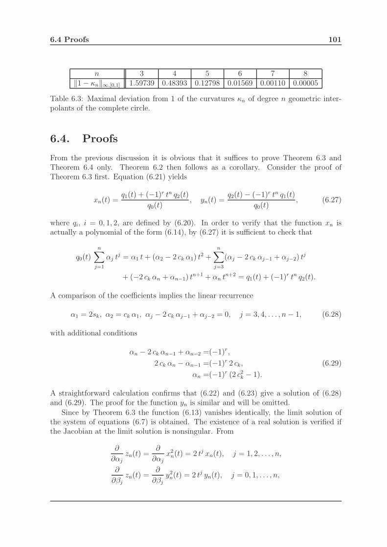
6.4 Proofs 101
n 3 4 5 6 7 8‖1 − κn‖∞,[0,1] 1.59739 0.48393 0.12798 0.01569 0.00110 0.00005
Table 6.3: Maximal deviation from 1 of the curvatures κn of degree n geometric inter-polants of the complete circle.
6.4. Proofs
From the previous discussion it is obvious that it suffices to prove Theorem 6.3 andTheorem 6.4 only. Theorem 6.2 then follows as a corollary. Consider the proof ofTheorem 6.3 first. Equation (6.21) yields
xn(t) =q1(t) + (−1)r tn q2(t)
q0(t), yn(t) =
q2(t) − (−1)r tn q1(t)
q0(t), (6.27)
where qi, i = 0, 1, 2, are defined by (6.20). In order to verify that the function xn isactually a polynomial of the form (6.14), by (6.27) it is sufficient to check that
q0(t)n∑
j=1
αj tj = α1 t+ (α2 − 2 ck α1) t
2 +n∑
j=3
(αj − 2 ck αj−1 + αj−2) tj
+ (−2 ck αn + αn−1) tn+1 + αn t
n+2 = q1(t) + (−1)r tn q2(t).
A comparison of the coefficients implies the linear recurrence
α1 = 2sk, α2 = ck α1, αj − 2 ck αj−1 + αj−2 = 0, j = 3, 4, . . . , n− 1, (6.28)
with additional conditions
αn − 2 ck αn−1 + αn−2 =(−1)r,
2 ck αn − αn−1 =(−1)r 2 ck, (6.29)
αn =(−1)r (2 c2k − 1).
A straightforward calculation confirms that (6.22) and (6.23) give a solution of (6.28)and (6.29). The proof for the function yn is similar and will be omitted.
Since by Theorem 6.3 the function (6.13) vanishes identically, the limit solution ofthe system of equations (6.7) is obtained. The existence of a real solution is verified ifthe Jacobian at the limit solution is nonsingular. From
∂
∂αjzn(t) =
∂
∂αjx2
n(t) = 2 tj xn(t), j = 1, 2, . . . , n,
∂
∂βjzn(t) =
∂
∂βjy2
n(t) = 2 tj yn(t), j = 0, 1, . . . , n,

102 Circle-like curves
it is straightforward to compute the Jacobian J := 2D, where
D :=
0 · · · · · · · · · 0 β0 0 · · · · · · 0 0
0 0 · · · · · · 0 β1 β0 0... 0
α1 0. . .
...... β1 β0
. . ....
...
α2 α1. . .
. . ....
...... β1
. . . 0...
... α2. . . 0 0
......
.... . . β0 0
......
. . . α1 0 βn...
.... . . β1 β0
αn... α2 α1 0 βn
...... β1
0 αn... α2
... 0 βn...
...... 0
. . ....
......
... 0. . .
......
......
. . . αn...
......
.... . . βn
...0 0 · · · 0 αn 0 0 0 · · · 0 βn
.
Unfortunately, obtaining the explicit formula for detD is not an easy task, since itsentries are given by (6.22)–(6.25). But the columns of D are simply the shifts of thecoefficients of xn and yn, which leads to the following observation. If
u0 := 0, u1, u2, . . . , u2n ∈ C
are 2n+ 1 pairwise distinct values, and
V (u0, u1, . . . , u2n) :=(uℓ−1
j−1
)2n+1
j,ℓ=1
is the corresponding Vandermonde matrix, then the rows of the product V D are givenby
uj xn(uj), u2j xn(uj), . . . , u
nj xn(uj), yn(uj), uj yn(uj), . . . , u
nj yn(uj), (6.30)
where j = 0, 1, . . . , 2n. Now (6.12) suggests how to choose uj, i.e., to define uj as 2ndifferent solutions of the equation
t2 n + 1 = 0. (6.31)
Then (6.12) implies xn(uj) = ±i yn(uj). Here i will denote the imaginary unit, i.e.,i2 = −1. If
uj := exp
(
(−1)r i π
2n(4 j − 3)
)
, j = 1, 2 . . . , n, j 6= j0,
uj0 := exp
(i π
2n(2 r − 1)
)
,
un+j := u−1j , j = 1, 2, . . . , n,
where
j0 =
{2n−r+2
2, r even,
r+12, r odd,

6.4 Proofs 103
then
yn(uj) = −i xn(uj), j = 1, 2, . . . , n,
yn(uj) = i xn(uj), j = n + 1, n+ 2, . . . , 2n, (6.32)
as can easily be verified. Recall that u0 = 0, yn(0) = 1, and use (6.30) and (6.32) to seethat
det(V D) = in2 n∏
j=1
xn(uj) detC,
where
C :=
0 0 · · · 0 1 0 · · · 0u1 u2
1 · · · un1 −1 −u1 · · · −un
1...
... · · · ......
... · · · ...un u2
n · · · unn −1 −un · · · −un
n
un+1 u2n+1 · · · un
n+1 1 un+1 · · · unn+1
un+2 u2n+2 · · · un
n+2 1 un+2 · · · unn+2
...... · · · ...
...... · · · ...
u2n u22 n · · · un
2 n 1 u2 n · · · un2n
.
Since J = 2D,
det J = 22 n+1 in2 n∏
j=1
xn(uj)detC
detV. (6.33)
LEMMA 6.5. If sk is given by (6.19), then
2 n∏
j=1
xn(uj) = n4 s4k.
Proof. Some straightforward computation and (6.27) yield
xn(uj)xn(un+j) =sin2
(π
4 n((−1)r(4 j − 3) + 2 r − 1)
)
sin2(
π4 n
((−1)r(4 j − 3) − 2 r + 1)) , j = 1, 2, . . . , n, j 6= j0,
and, by the L’Hospital rule,
xn(uj0) xn(un+j0) = n2 s2k. (6.34)
The formulae (see [20], e.g.)
n∏
j=1
sin( π
2n(2j − 2m− 1)
)
=(−1)m
2n−1, m ∈ Z,
n∏
j=1
j 6=m
sin( π
2n(2j − 2m)
)
=(−1)m+1n
2n−1, 1 ≤ m ≤ n,

104 Circle-like curves
imply2n∏
j=1j 6=j0, n+j0
xn(uj) = n2 s2k,
which, together with (6.34), completes the proof of the lemma.
LEMMA 6.6. The quotient of determinants in (6.33) is
detC
detV=
(−1)n r+1
in n2 s2k
.
Proof. The determinant of C can be reduced to
detC = (−1)n
2 n∏
j=1
uj det
(V1 −V1
V2 V2
)
,
where V1 := V (u1, u2, . . . , un) and V2 := V (un+1, un+2, . . . , u2n) are the correspondingVandermonde matrices. Since uj are the roots of (6.31),
∏2 nj=1 uj = 1. Further, a simple
columnwise reduction implies that
detC = (−1)n 2n detV1 detV2,
which finally givesdetC
detV= (−1)n 2n 1
∏nℓ=1
∏nj=1(un+ℓ − uj)
.
If
p1 :=n∏
ℓ=1ℓ 6=j0
n∏
j=1
j 6=j0
(un+ℓ − uj),
p2 := (un+j0 − uj0)n∏
j=1
j 6=j0
(un+j0 − uj)n∏
ℓ=1ℓ 6=j0
(un+ℓ − uj0),
then obviouslyn∏
ℓ=1
n∏
j=1
(un+ℓ − uj) = p1 p2.
A straightforward computation yields
p1 = (−1)n r in+1 2n−1 sk,
p2 = (−1)n n2 2 i sk,
thusdetC
detV=
(−1)n r+1
in n2 s2k
.
Lemma 6.6 and (6.33) confirm the result of Theorem 6.4 which concludes this sub-section.

6.5 Approximation of circular arcs 105
6.5. Approximation of circular arcs
In this subsection a generalization of the results obtained by Lyche and Mørken in [34]on the approximation of circular arcs by parametric polynomial curves of odd degrees isgiven. The results of the previous discussion are used to show that for the circular arcof the angular length h, a parametric polynomial curve of arbitrary degree n ∈ N, whichinterpolates a given arc at a particular point, can be constructed with a radial distancebounded by h2 n.
The approximation problem considered is the following. Let
AAAAAAAAA(ϕ) :=
(sinϕcosϕ
)
, 0 ≤ ϕ < L ≤ 2 π, (6.35)
be a particular parameterization of a circular arc of an angular length L. Find a para-metric polynomial curve
qqqqqqqqqn :=
(xn
yn
)
(6.36)
of degree ≤ n with nonconstant scalar polynomials xn, yn ∈ R[t] defined in (6.14), whichprovides “the best approximation” of (6.35). The only prescribed interpolation point isAAAAAAAAA(0) := (xn(0), yn(0))T := (0, 1)T . Note that it is enough to consider arcs of the unitcircle only, since any other arc of the same angular length can be obtained by affinetransformations.
The approximation error between a circular arc and a parametric polynomial curveis measured as a “radial distance” (see Figure 6.3), i.e.,
dr(AAAAAAAAA, qqqqqqqqqn) := maxt∈I
{∣∣∣
√
x2n(t) + y2
n(t) − 1∣∣∣
}
, (6.37)
where I is some interval of observation. If qqqqqqqqqn is a good approximation of AAAAAAAAA on I then(6.37) is small and
√
x2n(t) + y2
n(t) ≈ 1, thus
∣∣∣
√
x2n(t) + y2
n(t) − 1∣∣∣ =
|x2n(t) + y2
n(t) − 1|√
x2n(t) + y2
n(t) + 1≈ 1
2
∣∣x2
n(t) + y2n(t) − 1
∣∣ ,
and, for computational purposes, it is enough to consider only the “error”
e(t) :=∣∣x2
n(t) + y2n(t) − 1
∣∣ . (6.38)
Ideally, e would be zero if a polynomial parameterization of a circular arc would exist.But if at least one of xn or yn is of degree n, then
x2n(t) + y2
n(t) = (α2n + β2
n) t2 n + · · · 6= 1. (6.39)
Now it follows from (6.38) that e will be small (at least for small t), if coefficients at thelower degree terms in (6.39) will vanish. This implies that e will be as small as possibleif
x2n(t) + y2
n(t) = 1 + const · t2 n. (6.40)

106 Circle-like curves
-1 -0.5 0.5 1
-1
-0.5
0.5
1
Figure 6.3: Radial distance between a circular arc (solid) and a parametric curve ap-proximation (dashed).
Now, a proper reparameterization
t→ t2 n√
α2n + β2
n
transforms (6.40) to relation (6.12), and Theorem 6.3 (eq. (6.22)–(6.25)) gives the closed-form solution for the coefficients of polynomials xn and yn.
The approximation order is stated in the following lemma.
LEMMA 6.7. Let the circular arc AAAAAAAAA be defined by (6.35) and its parametric approx-imation qqqqqqqqqn by (6.36). Let the coefficients of xn and yn be given by (6.22)–(6.25). Ifqqqqqqqqqn : [0, h] → R2, where h is sufficiently small, then
dH(AAAAAAAAA, qqqqqqqqqn) ≤ dP (AAAAAAAAA, qqqqqqqqqn) ≤ dr(AAAAAAAAA, qqqqqqqqqn) ≤ h2 n,
where dr is defined by (6.37).
Proof. It is clear that for a particular θ, which is a regular reparameterization of AAAAAAAAA on[0, h],
dP (AAAAAAAAA, qqqqqqqqqn) ≤ maxt∈[0,h]
||AAAAAAAAA(θ(t)) − qqqqqqqqqn(t)||2.
Thus, it is enough to find a regular reparameterization θ of AAAAAAAAA for which
maxt∈[0,h]
||AAAAAAAAA(θ(t)) − qqqqqqqqqn(t)||2 ≤ h2 n.
Let θ : [0, h] → I be defined as
θ(t) := arctan
(xn(t)
yn(t)
)
. (6.41)

6.5 Approximation of circular arcs 107
Since xn(0) = 0, yn(0) = 1 and by (6.22) x′n(0) = 2 sk,
θ′(0) =x′n(0) yn(0) − xn(0) y′n(0)
x2n(0) + y2
n(0)= 2 sk > 0,
and there exists h0 > 0, such that θ is a regular reparameterization on [0, h] for 0 < h <h0. But a point (AAAAAAAAA ◦ θ)(t) lies on the circular arc defined by AAAAAAAAA and on the ray from theorigin to qqqqqqqqqn(t). This implies
||(AAAAAAAAA ◦ θ)(t) − qqqqqqqqqn(t)||2 = |√
x2n(t) + y2
n(t) − 1| ≤ |x2n(t) + y2
n(t) − 1| = t2 n,
where the last equality follows from (6.12). Finally,
maxt∈[0,h]
||(AAAAAAAAA ◦ θ)(t) − qqqqqqqqqn(t)||2 ≤ h2 n
and the proof of the lemma is complete.
An interesting question is, how large can be the angular length of the circular arc,which can be approximated by the previous method. First of all, the regularity of θhas to be assured, i.e., h has to be small enough. Then the angular length of thereparameterized circular arc AAAAAAAAA ◦ θ can be derived at least asymptotically.
LEMMA 6.8. If θ is a regular reparameterization on [0, h] defined by (6.41), then thelength of the circular arc AAAAAAAAA ◦ θ : [0, h] → R2 is 2 sk h+ O(h2).
Proof. The proof is straightforward. The regularity of θ, (6.12), (6.22)–(6.25) and thefact that (1 + t2 n)−1 = 1 + O(t2 n), simplify the arc-length to
s =
∫ h
0
‖(AAAAAAAAA ◦ θ)′(t)‖2 dt =
∫ h
0
|x′n(t) yn(t) − xn(t) y′n(t)|x2
n(t) + y2n(t)
dt
=
∫ h
0
x′n(t) yn(t) − xn(t) y′n(t)
1 + t2 ndt
=
∫ h
0
(x′n(t) yn(t) − xn(t) y′n(t))(1 + O(t2 n)) dt = 2 sk h+ O(h2).
Since we know that the best local approximation at a particular point in the functionalcase is the Taylor expansion, the natural question arises how good the approximationcan be, if xn and yn are taken as Taylor polynomials for sine and cosine at t = 0. Theresult is summarized in the following lemma.
LEMMA 6.9. Let xn and yn be the degree n Taylor polynomials of sine and cosine,respectively. Then
x2n(t) + y2
n(t) = 1 +1
wntm + O(tm+1),
where
m :=
{n+ 1, n is odd,n+ 2, n is even,

108 Circle-like curves
and
wn =
{m2n!, if nmod4 = 1, 2,
−m2n!, otherwise.
Proof. Let
Rs(t) = sin t− xn(t),
Rc(t) = cos t− yn(t),
be Lagrange remainders in Taylor expansions. Since
x2n(t) + y2
n(t) = 1 − 2(Rs(t) sin t+Rc(t) cos t) +R2s(t) +R2
c(t) (6.42)
and Rs, Rc are of order O(tn+1), it is enough to consider S(t) := −2(Rs(t) sin t +Rc(t) cos t) only.First, suppose that n is odd, i.e., n = 2 ℓ− 1. In this case the expansions of Rs and Rc
are
Rs(t) =(−1)ℓ
(n+ 2)!tn+2 + O(tn+4), Rc(t) =
(−1)ℓ
(n+ 1)!tn+1 + O(tn+3),
therefore
S(t) = −2(−1)ℓ
(n+ 1)!tn+1 + O(tn+3).
By (6.42), m = n + 1 and
wn =(−1)ℓ+1 (n+ 1)!
2.
If n is even, n = 2 ℓ,
Rs(t) =(−1)ℓ
(n+ 1)!tn+1 + O(tn+3), Rc(t) =
(−1)ℓ+1
(n+ 2)!tn+2 + O(tn+4),
thus
S(t) = −2
((−1)ℓ
(n+ 1)!tn+2 +
(−1)ℓ+1
(n + 2)!tn+2
)
+ O(tn+4).
Again by (6.42), m = n + 2 and
wn =(−1)ℓ+1 (n+ 2)n!
2.
The last lemma confirms that the Taylor polynomials are not an optimal choice ifthe radial distance is used as a measure of the approximation order.
Chapter 7
Resultants, Grobner basis andBrouwer’s degree
In this chapter the definition and some of the main properties of resultants, Grobnerbasis and Brouwer’s mapping degree are given. Further results can be found in [6], [1],[3], [5].
7.1. Resultants
A resultant is defined in the following way.
DEFINITION 7.1. Given a polynomial
p(x) = anxn + an−1x
n−1 + · · ·+ a1x+ a0
of degree n with zeros αi, i = 1, . . . , n, and a polynomial
q(x) = bmxm + bm−1x
m−1 + · · ·+ b1x+ b0
of degree m with zeros βj, j = 1, . . . , m, the resultant is defined by
Res(p, q; x) := amn b
nm
n∏
i=1
m∏
j=1
(αi − βj).
The resultant is also given by the determinant of the corresponding (n+m)×(n+m)

110 Resultants, Grobner basis and Brouwer’s degree
Sylvester matrix. Namely,
Res(p, q; x) = det
a0 b0a1 a0 b1 b0
a1. . . b1
. . ....
. . . a0...
. . . b0... a1
.... . . b1
an bm
an... bm
.... . .
. . .
an bm
.
It is clear that Res(p, q; x) = 0 if and only if p(x) and q(x) have a common factor in R[x].If p and q are polynomials of the same degree n = m, then there is another way to
compute their resultant. From the following polynomial in two variables
B(x, y) =p(x)q(y) − p(y)q(x)
x− y=
n−1∑
i,j=0
ci,jxiyj,
form a symmetric n × n matrix C := (ci,j)n−1i,j=0 (Bezout matrix). The determinant of
C (Bezout resultant) equals ±Res(p, q; x). Practical experience shows that the Bezoutmatrix is superior to the Sylvester matrix with regard to the numerical stability. So, ifone has two polynomials of the same large degree with numerical coefficients, then it isbetter to use the Bezout matrix.
Computing the resultant of two polynomials with respect to a specific variable is astandard feature in many computer algebra systems. These implementations make useof either the Sylvester matrix or the Bezout matrix, and they work quite fast.
There are many applications of the resultants. Resultants can be used to eliminatethe variables from the system of polynomial equations. Furthermore, one can use them tofind intersections of two algebraic curves in the real plane, for implicitization of rationalcurves in the plane, etc.
7.2. Grobner basis
Let K := k[x1, x2, . . . , xn] denote a ring of multivariate polynomials over k in variablesx1, x2, . . . , xn. Further, let
xxxxxxxxx = (x1, x2, . . . , xn), β = (β1, β2, . . . , βn), xxxxxxxxxβ = xβ1
1 xβ2
2 . . . xβn
n .
Every f ∈ K can be written as
f = a1xxxxxxxxxα1 + a2xxxxxxxxx
α2 + · · ·+ arxxxxxxxxxαr ,
where 0 6= ai ∈ k, and xxxxxxxxxα1 > xxxxxxxxxα2 > · · · > xxxxxxxxxαr with respect to some chosen monomialorder. Further let us denote the leading power product by lp(f) := xxxxxxxxxα1 . A Grobnerbasis is defined in the following way.

7.3 Brouwer’s mapping degree 111
DEFINITION 7.2. A set of nonzero polynomials G = {g1, g2, . . . , gℓ} contained insome ideal I ⊆ K is a Grobner basis for I if for every nonzero f ∈ I there existsi ∈ {1, 2, . . . , ℓ} such that the lp(gi) divides lp(f).
A Grobner basis G can also be characterized by one of the properties given in thenext theorem.
THEOREM 7.3. Let I ⊆ K be a nonzero ideal. The following statements are equivalentfor a set of nonzero polynomials G = {g1, g2, . . . , gℓ} ⊆ I.
(i) G is a Grobner basis for I.
(ii) Multivariate division (see [1]) of any polynomial in the ideal I by G gives 0.
(iii) f ∈ I if and only if f =∑ℓ
i=1 higi, where
lp(f) = max1≤i≤ℓ
{lp(hi) lp(gi)}.
(iv) The ideal given by the leading terms of polynomials in the ideal I is itself generatedby the leading terms of the basis G.
If G = {g1, g2, . . . , gℓ} is a Grobner basis of the ideal I, then I is generated by itselements, i.e., I = 〈g1, g2, . . . , gℓ〉. Furthermore, for every nonzero ideal I ⊆ K, generatedby a finite set of polynomials, a Grobner basis exists. One method for computing it isknown as Buchberger’s algorithm.
Since multivariate division requires a monomial ordering, the basis depends on thechosen monomial ordering, and different orderings can give rise to radically differentGrobner bases. Two of the most commonly used orderings are a lexicographic order,and a degree reverse lexicographic order. A lexicographic order eliminates variables, butresulting Grobner bases are often very large and expensive to compute. Degree reverselexicographic order typically provides the fastest Grobner basis computations.
A Grobner basis is called reduced if the leading coefficient of each element of the basisis 1 and no monomial in any element of the basis is in the ideal generated by the leadingterms of the other elements of the basis. The reduced Grobner basis is unique.
In the worst case, computation of the Grobner basis may require time that is expo-nential or even doubly-exponential in the number of solutions of the polynomial system.Most computer algebra systems contain routines to compute the Grobner basis.
Grobner bases with respect to the lexicographic order are very useful for solving poly-nomial equations and for elimination of variables. The set of polynomials in the Grobnerbasis have the same collection of roots as the original polynomials.
7.3. Brouwer’s mapping degree
Let U denote a bounded open subset of Rn. For a C1 mapping f : U → Rn, f =(f1, f2, . . . , fn), the Jacobian matrix at xxxxxxxxx ∈ U is
f ′(xxxxxxxxx) =
(∂fi
∂xj(xxxxxxxxx)
)n
i,j=1
,

112 Resultants, Grobner basis and Brouwer’s degree
and the Jacobian determinant is
Jf(xxxxxxxxx) = det f ′(xxxxxxxxx).
Further,RV(f ) =
{yyyyyyyyy ∈ R
n∣∣ ∀xxxxxxxxx ∈ f−1(yyyyyyyyy) : Jf(xxxxxxxxx) 6= 0
}
is the set of regular values. Its complement CV(f ) = Rn \ RV(f) is called the set ofcritical values.
Brouwer’s degree or simply a degree of a continuous mapping f on U is an integer,that gives some evidence on the number of zeros of f in U provided that f (xxxxxxxxx) 6= 0 on∂U . The precise definition is given in three parts.
(i) Suppose that f : U → Rn is a C1 mapping and yyyyyyyyy is a regular value. Then the degreeof f at yyyyyyyyy relative to U is
deg(f , U, yyyyyyyyy) =∑
x∈f−1(y)
sign Jf(xxxxxxxxx),
where the sum is finite and∑
x∈∅ = 0.
(ii) Suppose that f : U → Rn is a C1 mapping. Then one can find a sequence of regularpoints (yyyyyyyyyi)i that converge to yyyyyyyyy. The degree of f at yyyyyyyyy is then defined as
deg(f , U, yyyyyyyyy) = limi→∞
deg(f , U, yyyyyyyyyi).
(iii) If f is continuous in U , then there exists a sequence of C1 mappings (f i)i thatconverge to f uniformly on U , and
deg(f , U, yyyyyyyyy) = limi→∞
deg(f i, U, yyyyyyyyy).
It can be shown that the function deg(f , U, yyyyyyyyy) is well defined in (ii) and (iii), i.e., thelimits exist and are independent of the approximating sequences.
The basic properties of the degree function are the following:
1. deg(f , U, yyyyyyyyy) = deg(f − yyyyyyyyy, U, 0) (translation invariance).
2. Let H(xxxxxxxxx, t) be a continuous function of xxxxxxxxx ∈ U and t ∈ [0, 1], and suppose thatH(xxxxxxxxx, t) = yyyyyyyyy has no solution xxxxxxxxx ∈ ∂U for any t ∈ [0, 1]. Then deg(H(·, t), U, yyyyyyyyy) isconstant, independent of t ∈ [0, 1] (homotopy invariance).
3. deg(f , U, yyyyyyyyy) = deg(f , U, yyyyyyyyy′) for yyyyyyyyy and yyyyyyyyy′ in the same component of Rn \ f (∂U).
4. If U1 and U2 are open, disjoint subsets of U such that yyyyyyyyy 6∈ f (U \ (U1 ∪ U2)), thendeg(f , U, yyyyyyyyy) = deg(f , U1, yyyyyyyyy) + deg(f , U2, yyyyyyyyy) (additivity).
5. If U is a symmetric domain about the origin, f (−xxxxxxxxx) = −f (xxxxxxxxx) on ∂U , and f(xxxxxxxxx) 6= 0on ∂U . Then deg(f , U, 0) is an odd integer.
6. If deg(f , U, yyyyyyyyy) 6= 0, then the equation f(xxxxxxxxx) = yyyyyyyyy has solutions in U .

Bibliography
[1] W. W. Adams. P. Loustaunau: An introduction to Grobner bases. Graduate Studiesin Mathematics, 3. American Mathematical Society, Providence, RI, 1994.
[2] E. L. Allgower, K. Georg: Numerical continuation methods: an introduction.Springer Series in Computational Mathematics, 13. Springer-Verlag, Berlin, 1990.
[3] M. S. Berger: Nonlinearity and functional analysis. Lectures on nonlinear problemsin mathematical analysis. Pure and Applied Mathematics. Academic Press, NewYork-London, 1977.
[4] C. de Boor, K. Hollig, M. Sabin: High accuracy geometric Hermite interpolation.Comput. Aided Geom. Design 4, no. 4 (1987), 269–278.
[5] R. F. Brown: A topological introduction to nonlinear analysis. Birkhauser Boston,Inc., Boston, MA, 1993.
[6] D. Cox, J. Little, D. O’Shea: Using algebraic geometry. Graduate Texts in Mathe-matics, 185. Springer-Verlag, New York, 1998.
[7] W. L. F. Degen: High accurate rational approximation of parametric curves. Free-form curves and free-form surfaces (Oberwolfach, 1992). Comput. Aided Geom.Design 10, no. 3-4 (1993), 293–313.
[8] W. L. F. Degen: High accuracy approximation of parametric curves. Mathematicalmethods for curves and surfaces (Ulvik, 1994). Vanderbilt Univ. Press, Nashville,TN, (1995), 83–98.
[9] W. L. F. Degen: Geometric Hermite interpolation—in memoriam Josef Hoschek.Comput. Aided Geom. Design 22, no. 7 (2005), 573–592.
[10] T. Dokken, M. Dæhlen, T. Lyche, K. Mørken: Good approximation of circles bycurvature-continuous Bezier curves. Curves and surfaces in CAGD ’89 (Oberwolfach,1989). Comput. Aided Geom. Design 7, no. 1-4 (1990), 33–41.
[11] L. Fang: Circular arc approximation by quintic polynomial curves. Comput. AidedGeom. Design 15, no. 8 (1998), 843–861.
[12] L. Fang: G3 approximation of conic sections by quintic polynomial curves. Comput.Aided Geom. Design 16, no. 8 (1999), 755–766.
113

114 BIBLIOGRAPHY
[13] G. Farin: Curves and surfaces for computer-aided geometric design. A practicalguide. Academic Press, Inc., San Diego, CA, 1997.
[14] Y. Y. Feng and J. Kozak: On G2 continuous interpolatory composite quadraticBzier curves. J. Comput. Appl. Math. 72, no. 1 (1996), 141–159.
[15] Y. Y. Feng and J. Kozak: On G2 continuous cubic spline interpolation. BIT Nu-merical Mathematics 37, no. 2 (1997), 312–332.
[16] Y. Y. Feng and J. Kozak: On spline interpolation of space data. Mathematical meth-ods for curves and surfaces, II (Lillehammer, 1997). Innov. Appl. Math., VanderbiltUniv. Press, Nashville, TN, (1998), 167–174.
[17] M. Floater: High-order approximation of conic sections by quadratic splines. Com-put. Aided Geom. Design 12, no. 6 (1995), 617–637.
[18] M. S. Floater: An O(h2n) Hermite approximation for conic sections. Comput. AidedGeom. Design 14, no. 2 (1997), 135–151.
[19] M. Goldapp: Approximation of circular arcs by cubic polynomials. Comput. AidedGeom. Design 8, no. 3 (1991), 227–238.
[20] I. S. Gradsteın, I. M. Ryzik: Tablicy integralov, summ, ryadov i proizvedeniı (Rus-sian) (Tables of integrals, sums, series and products). Gosudarstv. Izdat. Tehn.-Teor.Lit., Moscow-Leningrad, 1951.
[21] K. Hollig, J. Koch: Geometric Hermite interpolation. Comput. Aided Geom. Design12, no. 6 (1995), 567–580.
[22] K. Hollig, J. Koch: Geometric Hermite interpolation with maximal order andsmoothness. Comput. Aided Geom. Design 13, no. 8 (1996), 681–695.
[23] G. Jaklic, J. Kozak, M. Krajnc, E. Zagar: On geometric interpolation by planarparametric polynomial curves. Math. Comput., 76, no. 260 (2007), 1981–1993.
[24] G. Jaklic, J. Kozak, M. Krajnc, E. Zagar: On geometric interpolation of circle-likecurves. Comput. Aided Geom. Design 24, no. 5 (2007), 241–251.
[25] G. Jaklic, J. Kozak, M. Krajnc, E. Zagar: Approximation of circular arcs by para-metric polynomial curves. Ann. Univ. Ferrara Sez. VII Sci. Mat. 53, no. 2 (2007),271–279.
[26] J. Kozak, M. Lokar: On piecewise quadratic G2 approximation and interpolation.Mathematical methods in computer aided geometric design, II (Biri, 1991). Aca-demic Press, Boston, MA, (1992), 359–366.
[27] J. Kozak, E. Zagar: On geometric interpolation by polynomial curves. SIAM J.Numer. Anal. 42, no. 3 (2004), 953–967.

BIBLIOGRAPHY 115
[28] J. Kozak, E. Zagar: Geometric interpolation of data in R3. Proceedings of theConference on Applied Mathematics and Scientific Computing. Springer, Dordrecht,(2005), 245–252.
[29] J. Kozak, M. Krajnc: Geometric interpolation by planar cubic polynomial curves.Comput. Aided Geom. Design 24, no. 2 (2007), 67–78.
[30] J. Kozak, M. Krajnc: Geometric interpolation by planar cubic G1 splines. BITNumerical Mathematics 47, no. 3 (2007), 547–563.
[31] M. Krajnc: Geometric Hermite interpolation by cubic G1 splines. Accepted in Non-linear Analysis: theory, methods and applications.
[32] C. Krattenthaler: Advanced determinant calculus. The Andrews Festschrift(Maratea, 1998). Sem. Lothar. Combin. 42 (1999).
[33] M. A. Lachance, A. J. Schwartz: Four-point parabolic interpolation. Comput. AidedGeom. Design 8, no. 2 (1991), 143–149.
[34] T. Lyche, K. Mørken: A metric for parametric approximation. Curves and surfacesin geometric design (Chamonix-Mont-Blanc, 1993). A K Peters, Wellesley, MA,(1994), 311–318.
[35] K. Mørken: Best approximation of circle segments by quadratic Bezier curves.Curves and surfaces (Chamonix-Mont-Blanc, 1990). Academic Press, Boston, MA,(1991), 331–336.
[36] K. Mørken: Parametric interpolation by quadratic polynomials in the plane. Math-ematical methods for curves and surfaces (Ulvik, 1994). Vanderbilt Univ. Press,Nashville, TN, (1995), 385–402.
[37] K. Mørken, K. Scherer: A general framework for high-accuracy parametric interpo-lation. Math. Comp. 66, no. 217 (1997), 237–260.
[38] A. Rababah: High order approximation method for curves. Comput. Aided Geom.Design 12, no. 1 (1995), 89–102.
[39] A. Rababah: High accuracy Hermite approximation for space curves in Rd. J. Math.Anal. Appl. 325, no. 2 (2007), 920–931.
[40] R. Schaback: On global GC2 convexity preserving interpolation of planar curves bypiecewise Bzier polynomials. Mathematical methods in computer aided geometricdesign (Oslo, 1988). Academic Press, Boston, MA, (1989), 539–547.
[41] R. Schaback: Interpolation with piecewise quadratic visually C2 Bzier polynomials.Comput. Aided Geom. Design 6, no. 3 (1989), 219–233.
[42] R. Schaback: Rational geometric curve interpolation. Mathematical methods incomputer aided geometric design, II (Biri, 1991). Academic Press, Boston, MA,(1992), 517–535.

116 BIBLIOGRAPHY
[43] R. Schaback: Planar curve interpolation by piecewise conics of arbitrary type. Con-str. Approx. 9, no. 4 (1993), 373–389.
[44] R. Schaback: Optimal geometric Hermite interpolation of curves. Mathematicalmethods for curves and surfaces, II (Lillehammer, 1997). Innov. Appl. Math., Van-derbilt Univ. Press, Nashville, TN, (1998), 417–428.
[45] K. Scherer: On local parametric approximation by polynomial curves. Approxima-tion theory (Witten, 1995), 86 (1995), 285–292.
[46] K. Scherer: Parametric polynomial curves of local approximation order 8. Curve andSurface Fitting (Saint Malo, 1999). Vanderbilt Univ. Press, Nashville, TN, (2000),375–384.
[47] E. Zagar: On G2 continuous spline interpolation of curves in Rd. BIT NumericalMathematics 42, no. 3 (2002), 670–688.

Index
admissible parameters, 5algorithm, 40
BackwardSplit, 42BackwardSweep, 42DivideAndConquer, 47ForwardSplit, 42ForwardSweep, 41
approximation order, 2, 70, 75arclength, 94asymptotic analysis, 75
Bezout resultant, 110boundary, 5breakpoint, 25, 55Brouwer’s degree, 12, 37, 67, 109Buchberger’s algorithm, 111
Chebyshev polynomial, 99circle-like curve, 93circular arc, 93Computer Aided Geometric Design, 93Computer Aided Manufacturing, 93Conjecture Hollig-Koch, 2continuation method, 1control polygon, 10convex data, 10curvature, 1cusp, 11
data constants, 10, 28, 59divided difference, 13
exponential spiral, 94
geometric continuity, 1geometric interpolation, 1Grobner basis, 7, 109
reduced, 111
Hausdorff distance, 2
higher order terms, 16homotopy, 20, 36, 67
ideal, 88elimination, 88
Implicit Function Theorem, 77, 97inflection point, 11interpolation problem
Hermite, 25, 55Lagrange, 4
Jacobian, 77, 97
L’Hospital rule, 103Lagrange scheme, 5logaritmic spiral, 6
monomial order, 110degree reverse lexicographic, 111lexicographic, 111
Newton method, 21Newton scheme, 5nonconvex data, 10
parameterizationchord length, 5rational, 98uniform, 5
parametric curvecubic polynomial, 9polynomial, 1rational, 93
parametric distance, 2planar scheme, 4
radial error, 93resultants, 22, 109
spline curve, 25
117

118 INDEX
G1, 25G2, 26
tangent direction, 1, 25, 55Taylor polynomial, 107
Vandermonde matrix, 104variety, 88

Razsirjeni povzetek
Geometrijska interpolacija s parametricnimi polinomskimi krivuljami in zlepki je bilaprvic predstavljena v [4], kjer je obravnavana Hermitova kubicna interpolacija dvehtock, smeri tangent in ukrivljenosti. Dokazano je, da je red pri aproksimaciji ravninskekonveksne krivulje sest, za razliko od funkcijskega primera, kjer je red le stiri. Visokred aproksimacije je le eden od razlogov, ki je k studiju geometrijskih aproksimacijskihshem privabil mnogo avtorjev. Drug pomemben razlog je ta, da je oblika geometri-jskih interpolantov v vecini primerov boljsa od oblike obicajnih funkcijskih interpolan-tov. Osnovni princip geometrijske interpolacije je, da krivulja ni odvisna od dejanskeparametrizacije, ampak le od geometrijskih kolicin, kot so tocke, smeri tangent, ukriv-ljenosti itd. Ker ne predpisemo nobenih dodatnih pogojev, kot so na primer parametri,pri katerih tocke interpoliramo, velikosti tangent ali ukrivljenosti, je red aproksimacijevisji kot pri obicajni funkcijski interpolaciji. Geometrijske sheme so zato pomembnoorodje v racunalnisko podprtem geometrijskem oblikovanju (CAGD). Glavni problemteh shem pa je, da vkljucujejo nelinearne enacbe, zato so vprasanja o obstoju resitve,redu aproksimacije in ucinkoviti implementaciji zelo tezka.
Obicajno krivulj ne aproksimiramo z eno samo polinomsko krivuljo, ampak s koncnimstevilom krivulj, ki se v sticnih tockah ujemajo z dolocenim redom geometrijske zveznosti.Pravimo, da sta dve krivulji G0 zvezni, ce se ujemata v skupni tocki, G1 zvezni, ce imatav skupni tocki isto smer tangente, G2 zvezni, ce imata v skupni tocki isto smer tangentein isto ukrivljenost, itd. V splosnem geometrijsko zveznost definiramo takole.
DEFINICIJA 1. Dve parametricni krivulji
fffffffff1 : [t0, t1] → Rd, fffffffff 2 : [s0, s1] → R
d,
se ujemata z geometrijsko zveznostjo reda k oziroma sta Gk-zvezni, ce se koncna tockafffffffff1 ujema z zacetno tocko fffffffff 2, fffffffff 1(t1) = fffffffff2(s0), in ce obstaja regularna reparametrizacijaφ : [t0, t1] → [s0, s1], da velja
djfffffffff 1
dtj(t)
∣∣∣∣t=t1
=dj(fffffffff 2 ◦ φ)
dtj(t)
∣∣∣∣t=t1
, j = 0, 1, . . . , k.
Za dolocanje reda aproksimacije moramo znati meriti razdalje med parametricnimiobjekti. Ker so ti najveckrat predstavljeni kot mnozice tock, je ena od moznih metrikzelo znana Hausdorfova razdalja.

120 Razsirjeni povzetek
DEFINICIJA 2. Naj bosta X in Y podmnozici metricnega prostora M . Hausdorfovarazdalja dH(X, Y ) je definirana kot
dH(X, Y ) := max
{
supx∈X
infy∈Y
d(x, y), supy∈Y
infx∈X
d(x, y)
}
,
kjer je d(x, y) razdalja v metricnem prostoru M .
Na zalost pa je Hausdorfovo razdaljo v praksi zelo tezko racunati. Za njeno zgornjomejo sta T. Lyche and K. Mørken ([34]) predlagala tako imenovano parametricno raz-daljo.
DEFINICIJA 3. Naj bosta fffffffff 1 in fffffffff2 dve parametricni krivulji, definirani na intervalihI1 in I2. Parametricna razdalja med fffffffff1 in fffffffff 2 je definirana kot
dist(fffffffff 1, fffffffff 2) := infφ‖fffffffff1 ◦ φ− fffffffff 2‖ = inf
φmaxt∈I2
‖fffffffff 1(φ(t)) − fffffffff 2(t)‖,
kjer je φ : I2 → I1 regularna reparametrizacija.
V [22] sta K. Hollig in J. Koch postavila naslednjo domnevo, ki v splosnem se nidokazana.
DOMNEVA 4. Pod ustreznimi genericnimi predpostavkami lahko polinomska krivuljastopnje n interpolira
m = n+ 1 +
⌊n− 1
d− 1
⌋
tock na gladki krivulji fffffffff ∈ Rd. Ta interpolacijska krivulja aproksimira fffffffff z redom aproksi-macije m, ko gredo razlike med interpoliranimi tockami proti nic.
Vecina objavljenih rezultatov o geometrijski interpolaciji je dobljenih s pomocjoasimptoticne analize. Glavni avtorji in njihova dela so C. de Boor, K. Hollig, M. Sabin,J. Koch ([4], [22], [21]), T. Lyche, K. Mørken, K. Scherer ([37], [45], [46], [34]), W. L. F. De-gen ([7], [8], [9]), A. Rababah ([38], [39]), Y. Y. Feng, J. Kozak, E. Zagar ([16], [15], [14],[26], [27], [28], [47]) in R. Schaback ([40], [41], [44], [42], [43]). V prakticnih primerih parezultati z asimptoticno analizo niso zadostni, saj morajo robustni algoritmi temeljiti napogojih, ki vnaprej zagotavljajo obstoj interpolantov. Takih rezultatov pa je zaenkratzelo malo. Razen posebnih primerov, kot so interpolacija kroznih lokov ([34] [10], [19][35], [17], [18], [11], [12]), je le nekaj rezultatov o geometrijskih pogojih, ki zagotavljajoobstoj resitve. Pogoji za obstoj parametricne parabole, ki interpolira stiri tocke, so po-dani v [33]. V [36] so ti pogoji razsirjeni na vse mozne primere (Taylorjev, Hermitov,Lagrangeev). Interpolacija poljubnega stevila tock v ravnini s parabolicnimi G2 zlepkije obravnavana v [41], [14], [26], kjer so izpeljani zadostni pogoji za obstoj in enolicnostresitve. Najbolj splosen rezultat sta dokazala J. Kozak in E. Zagar v [27], kjer sta izpel-jala potrebne in zadostne pogoje za obstoj interpolantov pri interpolaciji d+ 2 razlicnihtock v Rd s polinomsko krivuljo stopnje ≤ d.
V disertaciji obravnavam ravninske geometrijske sheme. Te so v praksi najboljuporabne, poleg tega pa je v ravnini razmik med parametricnim in funkcijskim primerom

Razsirjeni povzetek 121
najvecji. Domneva 4 namrec pravi, da lahko 2n ravninskih tock interpoliramo s polinom-sko krivuljo stopnje n in dosezemo red aproksimacije 2n, medtem ko lahko v funkcijskemprimeru polinomska krivulja stopnje n interpolira najvec n+1 tock z redom aproksimacijen+ 1.
Lagrangeev interpolacijski problem, na katerega se osredotocim, je naslednji: za danih2n ravninskih tock
TTTTTTTTT 0, TTTTTTTTT 1, . . . , TTTTTTTTT 2n−1 ∈ R2, TTTTTTTTT i 6= TTTTTTTTT i+1, (1)
poisci parametricno polinomsko krivuljo PPPPPPPPP n : [t0, t2n−1] → R2 stopnje ≤ n, ki interpoliradane tocke pri narascajocih vrednostih parametrov ti,
t0 < t1 < · · · < t2n−2 < t2n−1. (2)
Ker linearna transformacija domene parametrov ohranja stopnjo polinomske krivulje,lahko predpostavimo, da je t0 := 0 in t2n−1 := 1. Ostali parametri ttttttttt := (ti)
2n−2i=1 pa so
se neznani. Parametrom, ki zadoscajo (2), pravimo dopustni parametri. Nanje lahkogledamo kot na komponente tocke v odprtem simpleksu
Dn :={(ti)
2n−2i=1 ; 0 = t0 < t1 < · · · < t2n−2 < t2n−1 = 1
},
z robom ∂Dn, kjer vsaj dva razlicna ti sovpadata. Sistem enacb
PPPPPPPPP n(ti) = TTTTTTTTT i, i = 0, 1, . . . , 2n− 1, (3)
doloca tako krivuljo PPPPPPPPP n kot tudi neznane parametre ttttttttt. Nelinearni del je dolociti parame-tre. Ko jih izracunamo, dobimo koeficiente polinomske krivulje PPPPPPPPP n enostavno tako,da vzamemo katerihkoli n + 1 razlicnih interpolacijskih pogojev v (3) in na kompo-nentah PPPPPPPPP n uporabimo eno izmed standardnih interpolacijskih shem (Newtonova shema,Lagrangeeva shema).
Ker je sistem enacb (3) nelinearen, je dokaz eksistence dopustne resitve zelo tezekproblem. Resitev tudi ne obstaja nujno. Kot preprost primer vzemimo stiri tocke (n = 2)z nekonveksnim kontrolnim poligonom. Ker je vsaka komponenta interpolacijske krivuljePPPPPPPPP 2 parabola, ki ne more imeti vec kot dve nicli, je jasno, da interpolant ne more obstajati.Zelo lepi, potrebni in zadostni pogoji za obstoj resitve za n = 2 so dani v [27]. InterpolantPPPPPPPPP 2 obstaja natanko takrat, ko imajo determinante
det (∆TTTTTTTTT 0,∆TTTTTTTTT 1), det (∆TTTTTTTTT 0,∆TTTTTTTTT 2), det (∆TTTTTTTTT 1,∆TTTTTTTTT 2)
enak predznak. Tu je ∆TTTTTTTTT i := TTTTTTTTT i+1 − TTTTTTTTT i standardna oznaka za premo diferenco.Za motivacijo si oglejmo dva numericna primera. Najprej primerjajmo kubicno ge-
ometrijsko shemo s standardno interpolacijo s polinomi stopnje pet, kjer si za parametri-zacijo izberemo enakomerno ali tetivno parametrizacijo. Na slikah 1.1 se lepo vidi, da sekubicna krivulja (crna krivulja) dosti lepse prilega podatkom kot ostali dve. Racunskazahtevnost za izracun teh kubicnih interpolantov je zelo majhna. Newtonova metodaz ekvidistantnimi zacetnimi priblizki ti = i
5konvergira v povprecju v osmih iteracijah.
Kot naslednji primer aproksimirajmo logaritmicno spiralo
fffffffff(t) = log (t+ π)
(sin tcos t
)
, t ∈[
−π2,π
2
]
, (4)

122 Razsirjeni povzetek
z geometrijskimi interpolanti stopenj n = 3, 4, 5, 6. Podatke dobimo iz (4) z enakomernodelitvijo domene parametrov. Tabela 1.1 numericno potrjuje, da je red aproksimacije2n. Napako merimo kot parametricno razdaljo med krivuljo in njenim interpolantom.
Geometrijska interpolacija s kubicnimi polinomskimi krivuljami
V tem poglavju obravnavam Lagrangeevo interpolacijo sestih ravninskih tock s kubi-cno polinomsko krivuljo. Podani so zadostni geometrijski pogoji, ki zagotavljajo obstojinterpolanta PPPPPPPPP 3. Pogoji so precej preprosti in odvisni le od dolocenih determinant,izpeljanih iz danih tock.
Problem je naslednji: poiskati moramo pogoje, ki zagotavljajo obstoj vsaj ene do-pustne resitve nelinearnega sistema
PPPPPPPPP 3(ti) = TTTTTTTTT i, i = 0, 1, . . . , 5. (5)
Resitev je dopustna, ce parametri zadoscajo
0 =: t0 < t1 < · · · < t5 := 1. (6)
Pomembno vlogo igra matrika diferenc tock(∆TTTTTTTTT i
)4
i=0∈ R
2×5 in predznaki ter razmerjamed njenimi minorjiDi,j := det (∆TTTTTTTTT i,∆TTTTTTTTT j). To so predznacene ploscine paralelogramov,napetih na vektorje ∆TTTTTTTTT i,∆TTTTTTTTT j. Definirajmo se
λ1 :=D0,1
D1,2, λ2 :=
D0,2
D1,2, λ3 :=
D2,4
D2,3, λ4 :=
D3,4
D2,3, δ :=
D1,3
D1,2, µ :=
D2,3
D1,2,
γ1 :=λ2(1 + λ2)
λ1(1 + λ2) +√
λ1(1 + λ2)(λ1 + λ2),
γ2 :=λ3(1 + λ3)
λ4(1 + λ3) +√
λ4(1 + λ3)(λ3 + λ4).
Pri podatkih s konveksnim kontrolnim poligonom, kot na prvih treh slikah 1.1, je µ > 0in λi > 0, i = 1, 2, 3, 4. Kontrolni poligoni tock na zadnjih treh slikah 1.1 imajo prevojnotocko in zanje je µ < 0 in λi > 0, i = 1, 2, 3, 4. Omejimo se na studij takih podatkov.Geometrijska interpretacija λi, δ in µ je prikazana na sliki 2.1. Definirajmo se λλλλλλλλλ := (λi)
4i=1
in funkcije
ϑ1 (λλλλλλλλλ, µ) :=2µ− γ1 +
√
γ21 + 4µ(1 + γ1)
2γ1
,
ϑ2 (λλλλλλλλλ, µ) :=2 − µγ2 +
√
µ2γ22 + 4µ(1 + γ2)
2γ2,
ϑ3 (λλλλλλλλλ, µ) :=λ1µ
λ2+λ4
λ3+µ
λ2
√
λ1(λ1 + λ2)
1 + λ2,
ϑ4 (λλλλλλλλλ, µ) :=λ1µ
λ2+λ4
λ3+
1
λ3
√
λ4(λ3 + λ4)
1 + λ3,
ki bodo uporabljene v relacijah, ki zagotavljajo obstoj resitve. Glavna izreka sta nasled-nja:

Razsirjeni povzetek 123
IZREK 5. Naj bo D1,2D2,3 6= 0 in naj bodo podatki konveksni, to je µ > 0 in λi > 0,i = 1, 2, 3, 4. Ce sta bodisi ϑℓ enaka, ϑ1 (λλλλλλλλλ, µ) = ϑ2 (λλλλλλλλλ, µ), bodisi nista enaka in veljaeden od pogojev
δ < minℓ=1,2
{ϑℓ (λλλλλλλλλ, µ)} ali δ > maxℓ=1,2
{ϑℓ (λλλλλλλλλ, µ)} ,
potem kubicna interpolacijska krivulja PPPPPPPPP 3, ki zadosca (5), obstaja.
IZREK 6. Naj bo D1,2D2,3 6= 0 in naj ima kontrolni poligon tock prevoj, to je µ < 0 inλi > 0, i = 1, 2, 3, 4. Ce je
δ ∈ (ϑ3(λλλλλλλλλ, µ), ϑ4(λλλλλλλλλ, µ)) ,
potem kubicna interpolacijska krivulja PPPPPPPPP 3, ki zadosca (5), obstaja.
Izrek 5 in izrek 6 podata zadostne pogoje za obstoj kubicnega geometrijskega inter-polanta. Naslednji izrek pa izkljuci vecino podatkov, ki jih ta dva izreka ne pokrijeta.
IZREK 7. Pogoji na tocke, pri katerih resitev interpolacijskega problema (5) ne obstaja,so podani v tabeli 1.
D1,2D2,3 6= 0 D1,2D2,3 = 0µ > 0 µ < 0
λ2 ≤ 0, λ3 ≤ 0 λ2 ≤ 0 D1,2 = 0, D2,3 = 0δ ≤ 0, λ1 ≤ 0 λ3 ≤ 0 D1,2 = 0, λ3 ≤ 0δ ≤ 0, λ4 ≤ 0 λ1 ≤ 0, δ ≤ 0 D2,3 = 0, λ2 ≤ 0
λ1 ≤ 0, λ3 ≤ 0 , λ4 ≥ 0 λ4 ≤ 0, δ ≥ 0 D1,2 = 0, D0,1D2,3 ≥ 0λ2 ≤ 0, λ4 ≤ 0, λ1 ≥ 0 D2,3 = 0, D1,2D3,4 ≥ 0
Table 1: Pogoji na tocke, pri katerih resitev interpolacijskega problema (5) ne obstaja.
Se vedno pa ostane nekaj primerov, ki z izreki 5, 6 in 7 niso pokriti. Kot primervzemimo tocke
TTTTTTTTT 0 =
(−20 − ζ
3
)
, TTTTTTTTT 1 =
(−101
)
, TTTTTTTTT 2 =
(−50
)
, (7)
TTTTTTTTT 3 =
(50
)
, TTTTTTTTT 4 =
(101
)
, TTTTTTTTT 5 =
(20 + ζ
3
)
, ζ > 0,
za katere je λ1 = λ4 = − ζ10
, λ2 = λ3 = 2, δ = µ = 1. Ocitno niso izpolnjeni pogojinobenega od zgornjih izrekov. Ti podatki imajo za ζ ∈ (0, ζ0], kjer je ζ0 := 2.95373852,dve dopustni resitvi (slika 2.2). Pri ζ = ζ0 ti dve resitvi sovpadeta in krivulja ima spico,za ζ > ζ0 pa dopustna resitev ne obstaja vec.
Primeri na slikah 1.1 vsi zadoscajo pogojem izreka 5 ali izreka 6. Poglejmo si dvaizmed njih bolj natancno. Pri prvem primeru je δ < ϑ1 (λλλλλλλλλ, µ) < ϑ2 (λλλλλλλλλ, µ). Slika 2.3(levo) prikazuje, kako se spreminja polozaj tock, ko se δ priblizuje ϑ1 (λλλλλλλλλ, µ). Za δ ∈[ϑ1 (λλλλλλλλλ, µ) , ϑ2 (λλλλλλλλλ, µ)] dopustna resitev ne obstaja. Podobno nam slika 2.3 (desno) prikazujespreminjanje polozajev tock, ko gre δ od ϑ3 (λλλλλλλλλ, µ) do ϑ4 (λλλλλλλλλ, µ) za zadnji primer s slike 1.1.

124 Razsirjeni povzetek
Za δ < ϑ3 (λλλλλλλλλ, µ) ali δ > ϑ4 (λλλλλλλλλ, µ) lahko obstajata dve dopustni resitvi, zgodi pa sepodoben problem kot pri zgornjem primeru.
Pogoji izrekov 5 in 6 so zelo preprosti, v dokazu pa je potrebnih kar nekaj korakov.Poglejmo si idejo in skico dokaza. Sistem (5) najprej pretvorimo v obliko, ki je boljprimerna za nadaljno analizo. Locimo enacbe za neznane koeficiente od enacb za nez-nane parametre. To naredimo tako, da na sistemu (5) uporabimo deljene diference[tℓ, tℓ+1, . . . , tℓ+4], ki vsak kubicni polinom PPPPPPPPP 3 preslikajo v nic. Dobimo enacbe
ℓ+4∑
i=ℓ
1
ωℓ,ℓ+4(ti)TTTTTTTTT i = 000000000, ℓ = 0, 1, (8)
kjer je
ωi,j(t) := (t− ti)(t− ti+1) · · · (t− tj−1)(t− tj), ωi,j(t) =d
dtωi,j(t), i < j.
Nekaj enostavnih transformacij sistema (8) nam da koncni sistem enacb za neznaneparametre, ki se glasi
1
ω0,4(t0)(1 + λ2) +
1
ω0,4(t1)+
1
ω0,4(t4)µ = 0, (9)
1
ω0,4(t0)λ1 +
1
ω0,4(t3)+
1
ω0,4(t4)(1 + δ) = 0, (10)
1
ω1,5(t1)
(
1 +δ
µ
)
+1
ω1,5(t2)+
1
ω1,5(t5)λ4 = 0, (11)
1
ω1,5(t1)
1
µ+
1
ω1,5(t4)+
1
ω1,5(t5)(1 + λ3) = 0. (12)
V naslednjem koraku dokazemo, da parametri ti ne morejo biti pri nobeni resitvi, kizadosca (6), poljubno blizu roba ∂D3. To pove naslednji izrek, katerega dokaz je tehnicnoprecej zapleten, je pa to najpomembnejsi del v dokazu glavnih izrekov.
IZREK 8. Naj bodo izpolnjeni pogoji izreka 5 ali izreka 6. Potem sistem (9) - (12) nemore imeti nobene resitve poljubno blizu roba obmocja ∂D3.
Sledi dokaz, da ima nelinearni sistem za posebne podatke liho stevilo dopustnihresitev. To dejstvo nato razsirimo na splosni sistem s pomocjo homotopije in Brouwer-jevega izreka. In sicer definiramo homotopijo HHHHHHHHH(ttttttttt; ζ), ki nam da pri ζ = 0 sistem zaposebne, pri ζ = 1 pa sistem za splosne podatke. Dokazemo, da HHHHHHHHH(ttttttttt; ζ) = 000000000 zadoscapogojem izreka 8 za vsak ζ ∈ [0, 1]. Zato obstaja kompaktna mnozica K ⊂ D3, da velja
V := {ttttttttt ∈ D3; HHHHHHHHH(ttttttttt, ζ) = 000000000} ⊂ K ⊂ D3, V ∩ ∂K = ∅.
Ker torej HHHHHHHHH ni nic na robu K za noben ζ ∈ [0, 1], je Brouwerjeva stopnja invariantnaza ζ ∈ [0, 1]. Ker pa je liha za posebne podatke, mora imeti sistem vsaj eno dopustnoresitev.

Razsirjeni povzetek 125
Geometrijska interpolacija s kubicnimi G1 zlepki
V tem poglavju je obravnavana geometrijska interpolacija stirih tock in dveh smeritangent ter interpolacija s kubicnimi G1 zlepki. Dolocen je sirok razred zadostnih pogo-jev, ki zagotavljajo obstoj interpolantov in pokrijejo tako konveksne kot nekonveksnepodatke. Eksistencni pogoji so odvisni le od geometrije podatkov in so enostavno pre-verljivi. Dodan je tudi algoritem, s katerim dolocimo obmocja za smeri tangent, ce le teniso vnaprej predpisane.
Interpolacijski problem je sledec. Za dano zaporedje tock
TTTTTTTTT i ∈ R2, i = 0, 1, 2, . . . , 3m, TTTTTTTTT i 6= TTTTTTTTT i+1,
poisci kubicno G1 krivuljo zlepkov SSSSSSSSS : [a, b] → R2 s sticnimi tockami
a := u0 < u1 < · · · < um := b,
ki interpolira dane tocke TTTTTTTTT i, tako da
SSSSSSSSS(uℓ) = TTTTTTTTT 3ℓ, ℓ = 0, 1, . . . , m.
Z ddddddddd3ℓ, ‖ddddddddd3ℓ‖2 = 1, oznacimo smeri tangent krivulje SSSSSSSSS v uℓ. Z odsekoma polinomskopredstavitvijo
PPPPPPPPP ℓ(tℓ)
:= SSSSSSSSS(u)
[uℓ−1,uℓ], tℓ :=
u− uℓ−1
∆uℓ−1∈ [0, 1], ℓ = 1, 2, . . . , m,
se interpolacijski problem glasi takole: poisci kubicne polinomske krivulje PPPPPPPPP ℓ, za katerevelja
PPPPPPPPP ℓ(tℓi)
= TTTTTTTTT 3(ℓ−1)+i, i = 0, 1, . . . , 3,
d
dtℓPPPPPPPPP ℓ(0) = αℓ
0ddddddddd3(ℓ−1),d
dtℓPPPPPPPPP ℓ(1) = αℓ
3ddddddddd3ℓ,ℓ = 1, 2, . . . , m, (13)
kjer parametri tℓ1, tℓ2, α
ℓ0, α
ℓ3 zadoscajo
0 =: tℓ0 < tℓ1 < tℓ2 < tℓ3 := 1, αℓ0 > 0, αℓ
3 > 0, ℓ = 1, 2, . . . , m.
Smeri tangent ddddddddd3ℓ, ℓ = 1, 2, . . . , m−1, zaenkrat se niso predpisane, zato nas zanima tudi,kako dolociti obmocja za (dddddddddℓ)
mℓ=1, ki zagotavljajo obstoj resitve sistema enacb (13).
Poglejmo si najprej analizo enega odseka, torej m = 1 in PPPPPPPPP 1 =: PPPPPPPPP . Naj velja
ddddddddd0 := ddddddddd10, ddddddddd3 := ddddddddd1
3, t1 := t11, t2 := t12, α0 := α10, α3 := α1
3.
Nelinearen del interpolacijskega problema (13) je izracunati dopustne parametre(t1, t2, α0, α3) ∈ U , kjer je
U := {(t1, t2); 0 =: t0 < t1 < t2 < t3 := 1} × {(α0, α3); α0 > 0, α3 > 0} .

126 Razsirjeni povzetek
Ce na enacbah (13) uporabimo deljene diference, ki preslikajo kubicne polinome v nic,dobimo naslednji nelinearen sistem za (t1, t2, α0, α3):
[t0, t0, t1, t2, t3]PPPPPPPPP = 000000000 =α0
ω0,3(t0)ddddddddd0 +
3∑
j=1
(3∑
i=j
1
ω0,3(ti)
1
ti − t0
)
∆TTTTTTTTT j−1,
[t0, t1, t2, t3, t3]PPPPPPPPP = 000000000 =α3
ω0,3(t3)ddddddddd3 +
2∑
j=0
(j∑
i=0
1
ω0,3(ti)
1
t3 − ti
)
∆TTTTTTTTT j .
Z nekaj preprostimi transformacijami se ga da prepisati v
1
t21(1 − t1)− 1
t22(1 − t2)(1 + µ1) +
t2 − t1(1 − t1)(1 − t2)
(
1 + µ1(1 + λ1) −λ1
λ2
)
= 0,
1
t2(1 − t2)2− 1
t1(1 − t1)2(1 + µ2) +
t2 − t1t1t2
(
1 + µ2(1 + λ2) −λ2
λ1
)
= 0, (14)
in
α0 = δ1t1t2t2 − t1
(1
t22(1 − t2)− t2 − t1
(1 − t1)(1 − t2)(1 + λ1)
)
, (15)
α3 = δ2(1 − t1)(1 − t2)
t2 − t1
(1
t1(1 − t1)2− t2 − t1
t1t2(1 + λ2)
)
, (16)
kjer so nove konstante definirane z
λ2ℓ−1 :=D3ℓ−3,3ℓ−1
D3ℓ−3,3ℓ−2
, λ2ℓ :=D3ℓ−3,3ℓ−1
D3ℓ−2,3ℓ−1
,
µ2ℓ−1 :=det (ddddddddd3ℓ−3,∆TTTTTTTTT 3ℓ−2)
det (ddddddddd3ℓ−3,∆TTTTTTTTT 3ℓ−3), µ2ℓ :=
det (∆TTTTTTTTT 3ℓ−2, ddddddddd3ℓ)
det (∆TTTTTTTTT 3ℓ−1, ddddddddd3ℓ),
δ2ℓ−1 :=D3ℓ−3,3ℓ−2
det (ddddddddd3ℓ−3,∆TTTTTTTTT 3ℓ−3), δ2ℓ :=
D3ℓ−2,3ℓ−1
det (∆TTTTTTTTT 3ℓ−1, ddddddddd3ℓ).
Da poenostavimo analizo, predpostavimo λk > 0, µk > 0 in δk > 0, k = 1, 2, za konveksnepodatke in λ1 · λ2 < 0, δk > 0 za nekonveksne, to je podatke s prevojno tocko. Naslednjidve lemi povesta, kdaj je odvod PPPPPPPPP ′ v krajiscih intervala enak nic.
LEMA 9. Naj bo λ1 > 0. Tedaj obstaja enolicna resitev sistema (14) in (15), ki zadosca0 < t1 < t2 < 1 in pri kateri je α0 = 0, natanko tedaj, ko je λ2 > 0 in µ2 = φ2(λ1, λ2),kjer je
φ2(λ1, λ2) :=
λ21 − t1
t22− λ1
t1
(1 − t2)2
λ21 − t2
t21− λ1
t2
(1 − t1)2
− 1,
in je(t1, t2
)enolicna resitev sistema
1 − t1t22(t2 − t1)
= 1 + λ1,1 − t2
t21(t2 − t1)=λ1
λ2(1 + λ2) , 0 < t1 < t2 < 1.

Razsirjeni povzetek 127
LEMA 10. Naj bo λ1 > 0. Tedaj obstaja enolicna resitev sistema (14) in (16), kizadosca 0 < t1 < t2 < 1 in pri kateri je α3 = 0, natanko tedaj, ko je λ2 > 0 inµ1 = φ1(λ1, λ2) := φ2(λ2, λ1).
Definirajmo se funkciji
φ3(λ1, λ2, µ1) :=λ2µ1
λ1(λ2µ1 − 1 −√1 + µ1)
,
φ4(λ1, λ2, µ1) :=λ2µ1(λ2µ1(1 + 2λ1) − 2λ1)
λ21(λ2µ1 − 1)2
.
Naslednja dva izreka podata zadostne pogoje na podatke, ki implicirajo obstoj inter-polanta PPPPPPPPP . Prvi pokrije konveksne, drugi pa nekonveksne podatke.
IZREK 11. Naj podatki ddddddddd0, TTTTTTTTT 0, TTTTTTTTT 1, TTTTTTTTT 2, TTTTTTTTT 3, ddddddddd3 zadoscajo
λk > 0, δk > 0, µk > 0, k = 1, 2.
Ce je0 < µ1 < φ1(λ1, λ2) in 0 < µ2 < φ2(λ1, λ2),
aliµ1 > φ1(λ1, λ2) in µ2 > φ2(λ1, λ2),
potem kubicna interpolacijska krivulja PPPPPPPPP , ki zadosca (13), obstaja.
IZREK 12. Naj podatki ddddddddd0, TTTTTTTTT 0, TTTTTTTTT 1, TTTTTTTTT 2, TTTTTTTTT 3, ddddddddd3 zadoscajo
λ1 > 0, λ2 < 0, δ1 > 0 in δ2 > 0.
Ce je µ1 > 0 inφ3(λ1, λ2, µ1) < µ2 < φ4(λ1, λ2, µ1),
potem kubicna interpolacijska krivulja PPPPPPPPP , ki zadosca (13), obstaja.
OPOMBA 13. Iz simetrije v enacbah (14)-(16) sledi, da izrek 12 velja tudi, ce zamen-jamo vlogi λ1 in λ2 ter vlogi µ1 in µ2.
Geometrijska interpretacija izrekov 11 in 12 je prikazana na slikah 3.4 in 3.5. Idejadokaza je podobna kot v prejsnjem poglavju. Najprej dokazemo, da pod pogoji izrekovsistem (14)–(16) ne more imeti nobene resitve poljubno blizu roba ∂U . V naslednjemkoraku pokazemo, da imajo posebni podatki, ki zadoscajo pogojem izrekov, liho steviloresitev. Nato to dejstvo prenesemo na splosne podatke s pomocjo homotopije in Brouw-erjeve stopnje.
Poglejmo si sedaj interpolacijo z G1 kubicnimi zlepki ob predpostavki, da so smeritangent ddddddddd3ℓ neznane. Vsaka smer tangente je odvisna le od enega parametra. Ce stavektorja ∆TTTTTTTTT 3ℓ−1 in ∆TTTTTTTTT 3ℓ nekolinearna, smeri tangent izrazimo kot
ddddddddd0 := ddddddddd0(ξ0) := (ξ0 − 1)∆TTTTTTTTT 1 + ξ0∆TTTTTTTTT 0,
ddddddddd3ℓ := ddddddddd3ℓ(ξℓ) := σ3ℓ(1 − ξℓ)∆TTTTTTTTT 3ℓ−1 + σ3ℓ−1ξℓ∆TTTTTTTTT 3ℓ,
ddddddddd3m := dddddddddm(ξm) := (1 − ξm)∆TTTTTTTTT 3m−1 − ξm∆TTTTTTTTT 3m−2,
ℓ = 1, . . . , m− 1,

128 Razsirjeni povzetek
kjer je σk := sign
(Dk−1,k
Dk,k+1
)
. Ceprav tako predstavljene tangente niso normalizirane,
to ne spremeni eksistencnih pogojev. Po predpostavkah v eksistencnih izrekih morajobiti konstante δ2ℓ(ξℓ) > 0 in δ2ℓ+1(ξℓ) > 0 pozitivne. To je res, ce ξℓ lezi na intervalu(0, 1). Preprosto se da dolociti tudi podinterval v (0, 1), kjer sta pozitivna tudi µ2ℓ−1(ξ)in µ2ℓ(ξ). Rekli bomo, da je neka izbira parametrov (ξℓ)
mℓ=0 dopustna, ce so na vsakem
polinomskem odseku izpolnjeni pogoji izreka 11 ali izreka 12. Algoritem ForwardSweep,ki je predstavljen v disertaciji, vrne mnozico vektorjev intervalov ΞΞΞΞΞΞΞΞΞ = {Ξ0,Ξ1, . . . ,Ξm},za katere velja naslednje: za vsak r, 0 ≤ r ≤ m, in poljubno izbran ξr ∈ Ξr obstaja vsajena dopustna izbira
(ξ0, . . . , ξr−1, ξr, ξr+1, . . . , ξm) , ξℓ ∈ Ξℓ.
Kadar so podatki na vsakem odseku konveksni, to je
λ2ℓ−1 > 0, λ2ℓ > 0, ℓ = 1, 2, . . . , m,
pa velja mnogo mocnejsi rezultat. Ce je ΞΞΞΞΞΞΞΞΞ vektor intervalov, ki ga vrne algoritem, potemje poljubna izbira parametrov
(ξ0, ξ1, . . . , ξm) , ξℓ ∈ Ξℓ,
dopustna. Algoritem je preprost algoritem sestopanja, ki pregleda podatke najprej v enosmer TTTTTTTTT 0 → TTTTTTTTT 3m in doloci vmesni rezultat Ξℓ, ℓ = 0, 1, . . . , m, ki je tak, da za poljubenξℓ ∈ Ξℓ obstaja izbira ξi ∈ Ξi, i = 0, 1, . . . , ℓ − 1, da je (ξ0, ξ1, . . . , ξℓ) dopustna izbiraza tocke TTTTTTTTT i, i = 0, 1, . . . , 3ℓ. Korak v nasprotno smer TTTTTTTTT 3m → TTTTTTTTT 0 skrci trenutne Ξℓ,ℓ = m− 1, m− 2, . . . , 0, tako da za vsak ξℓ ∈ Ξℓ obstaja izbira
ξi ∈ Ξi, i = 0, 1, . . . , ℓ− 1, ℓ+ 1, . . . , m,
da je (ξ0, ξ1, . . . , ξm) dopustna za vse podatke. Ko enkrat imamo dolocene meje ΞΞΞΞΞΞΞΞΞ,moramo izbrati dejanske smeri tangent, to je izbrati ξℓ ∈ Ξℓ. Predstavljen je preprostalgoritem deli in vladaj, s katerim iz neprazne ΞΞΞΞΞΞΞΞΞ vedno dobimo dopustno izbiro. S temalgoritmom pa lahko tudi preverimo ali ima interpolacijski problem (13) resitev, kadarso smeri tangent predpisane vnaprej.
Hermitova geometrijska interpolacija s kubicnimi G1 zlepki
V tem poglavju obravnavam Hermitovo geometrijsko interpolacijo z ravninskimi ku-bicnimi G1 zlepki. Na vsakem polinomskem odseku interpoliram tri tocke in tri smeritangent. Podani so zadostni geometrijski pogoji za obstoj resitve, ki pokrijejo vecinoprimerov.
Problem je sledec. Za danih 2m+ 1 tock in smeri tangent
TTTTTTTTT i ∈ R2, dddddddddi ∈ R
2, TTTTTTTTT i 6= TTTTTTTTT i+1, ‖dddddddddi‖2 = 1, i = 0, 1, . . . , 2m,

Razsirjeni povzetek 129
poisci kubicno G1 krivuljo zlepkov SSSSSSSSS : [0, 1] → R2 s predpisanimi sticnimi tockami(t2i)
mi=0,
0 =: t0 < t1 < · · · < t2m−1 < t2m := 1,
ki interpolira tocke TTTTTTTTT i in smeri tangent dddddddddi pri parametrih ti,
SSSSSSSSS(ti) = TTTTTTTTT i,1
‖SSSSSSSSS′(ti)‖2SSSSSSSSS ′(ti) = dddddddddi, i = 0, 1, . . . , 2m, (17)
kjer so (t2i−1)mi=1 neznanke. Interpolacijska shema je ocitno lokalna, saj sprememba ene
tocke ali smeri tangente vpliva le na odsek, ki podatek vsebuje. Analizo in vse izracunelahko zato naredimo lokalno. Za m = 1 je zlepek SSSSSSSSS kar polinom, ki ga oznacimo s PPPPPPPPP .Enacbe za polinomski problem se dajo prepisati v
PPPPPPPPP (ti) = TTTTTTTTT i, PPPPPPPPP ′(ti) = αidddddddddi, αi > 0, i = 0, 1, 2, (18)
kjer mora veljati 0 := t0 < t1 < t2 := 1. Preostane nam torej dvanajst enacb za osemneznanih koeficientov krivulje PPPPPPPPP in stiri neznane parametre t1, α0, α1 in α2. Da lahkopodamo glavne eksistencne izreke, potrebujemo se nekaj oznak. Definirajmo konstante
λ1 :=det (ddddddddd0,∆TTTTTTTTT 0)
det (∆TTTTTTTTT 0,∆TTTTTTTTT 1), λ2 :=
det (∆TTTTTTTTT 0, ddddddddd1)
det (∆TTTTTTTTT 0,∆TTTTTTTTT 1),
λ3 :=det (ddddddddd1,∆TTTTTTTTT 1)
det (∆TTTTTTTTT 0,∆TTTTTTTTT 1), λ4 :=
det (∆TTTTTTTTT 1, ddddddddd2)
det (∆TTTTTTTTT 0,∆TTTTTTTTT 1),
µ1 :=det (ddddddddd0,∆TTTTTTTTT 1)
det (∆TTTTTTTTT 0,∆TTTTTTTTT 1), µ2 :=
det (∆TTTTTTTTT 0, ddddddddd2)
det (∆TTTTTTTTT 0,∆TTTTTTTTT 1)
in funkcije
ϕ1(λλλλλλλλλ, µ2) :=2λ1λ3λ4
λ3µ2 − λ2λ4, ϕ2(λλλλλλλλλ, µ1) :=
2λ1λ2λ4
λ2µ1 − λ1λ3
ψ1(λλλλλλλλλ) := λ1τ(λ3, λ2)
2(3 − 2τ(λ3, λ2))
(1 − τ(λ3, λ2))2(1 + 2τ(λ3, λ2)),
ψ2(λλλλλλλλλ) := λ4τ(λ2, λ3)
2(3 − 2τ(λ2, λ3))
(1 − τ(λ2, λ3))2(1 + 2τ(λ2, λ3)),
ψ3(λ1, λ4, µ1) := −λ4(3 − τ(−λ1, µ1)) τ(−λ1, µ1)
2
(1 − τ(−λ1, µ1))3 ,
ψ4(λ1, λ4, µ) := ψ3(λ4, λ1, µ),
kjer je τ(λ2, λ3) definiran kot enolicna resitev problema
g(t1;λ2, λ3) :=1
λ2
t211 − t1
− 1
λ3
(1 − t1)(2 + t1)
t1= 0, 0 < t1 < 1.
Zadostni pogoji za obstoj interpolacijske polinomske krivulje so naslednji:
IZREK 14. Naj podatki TTTTTTTTT i, dddddddddi, i = 0, 1, 2, zadoscajo det (∆TTTTTTTTT 0,∆TTTTTTTTT 1) 6= 0 in λλλλλλλλλ > 0. Cevelja katerakoli od naslednjih moznosti
130 Razsirjeni povzetek
1. µ1 > ψ1(λλλλλλλλλ) in µ2 > ψ2(λλλλλλλλλ),
2. λ1λ3
λ2≤ µ1 < ψ1(λλλλλλλλλ) in µ2 < ψ2(λλλλλλλλλ),
3. λ2λ4
λ3≤ µ2 < ψ2(λλλλλλλλλ) in µ1 < ψ1(λλλλλλλλλ),
4. −λ1λ3
λ2< µ1 <
λ1λ3
λ2in ϕ2(λλλλλλλλλ, µ1) < µ2 < ψ2(λλλλλλλλλ),
5. −λ2λ4
λ3< µ2 <
λ2λ4
λ3in ϕ1(λλλλλλλλλ, µ2) < µ1 < ψ1(λλλλλλλλλ),
potem kubicna interpolacijska krivulja PPPPPPPPP , ki zadosca (18), obstaja.
IZREK 15. Naj podatki TTTTTTTTT i, dddddddddi, i = 0, 1, 2, zadoscajo det (∆TTTTTTTTT 0,∆TTTTTTTTT 1) 6= 0, λi > 0,i = 1, 2, 3, in λ4 < 0. Ce velja
µ1 > ψ1(λλλλλλλλλ) in µ2 > ϕ2(λλλλλλλλλ, µ1) ali
λ1λ3
λ2< µ1 < ψ1(λλλλλλλλλ) in µ2 < ϕ2(λλλλλλλλλ, µ1),
potem kubicna interpolacijska krivulja PPPPPPPPP , ki zadosca (18), obstaja.
OPOMBA 16. Primer, ko je λ1 < 0 in λi > 0, i = 2, 3, 4, je simetricen primeru izizreka 15. Velja naslednje: ce je
µ2 > ψ2(λλλλλλλλλ) in µ1 > ϕ1(λλλλλλλλλ, µ2) ali
λ2λ4
λ3
< µ2 < ψ2(λλλλλλλλλ) in µ1 < ϕ1(λλλλλλλλλ, µ2),
potem kubicna interpolacijska krivulja PPPPPPPPP , ki zadosca (18), obstaja.
IZREK 17. Naj podatki TTTTTTTTT i, dddddddddi, i = 0, 1, 2, zadoscajo det (∆TTTTTTTTT 0,∆TTTTTTTTT 1) 6= 0 in λ1 > 0,λ2 > 0, λ3 < 0, λ4 < 0. Ce je
−λ1λ3
λ2< µ1 in ϕ2(λλλλλλλλλ, µ1) < µ2 <
λ2λ4
λ3+
2λ1λ4
µ1,
potem kubicna interpolacijska krivulja PPPPPPPPP , ki zadosca (18), obstaja.
OPOMBA 18. Primer, ko je λ1 < 0, λ2 < 0, λ3 > 0, λ4 > 0, je simetricen primeru izizreka 17. Rezultat je sledec. Ce je
−λ2λ4
λ3< µ2 in ϕ1(λλλλλλλλλ, µ2) < µ1 <
λ1λ3
λ2+
2λ1λ4
µ2,
potem kubicna interpolacijska krivulja PPPPPPPPP , ki zadosca (18), obstaja.
IZREK 19. Naj podatki TTTTTTTTT i, dddddddddi, i = 0, 1, 2, zadoscajo det (∆TTTTTTTTT 0,∆TTTTTTTTT 1) 6= 0 in λ1 < 0,λ4 < 0, µ1 > 0. Ce velja katerakoli od naslednjih moznosti
1. λ2 > 0, λ3 > 0, µ2 > ψ3(λ1, λ4, µ1),

Razsirjeni povzetek 131
2. λ2 < 0, λ3 > 0, 0 < µ1 ≤ λ1λ3
λ2, µ2 > ψ3(λ1, λ4, µ1),
3. λ2 > 0, λ3 < 0, 0 < µ2 ≤ λ2λ4
λ3, µ1 > ψ4(λ1, λ4, µ2),
4. λ2 < 0, λ3 < 0, µ1 > −λ1λ3
λ2, ϕ2(λλλλλλλλλ, µ1) < µ2 < ψ3(λ1, λ4, µ1),
5. λ2 < 0, λ3 < 0, 0 < µ1 ≤ −λ1λ3
λ2, 2λ1λ3λ4+λ2λ4µ1
λ3µ1< µ2 < ψ3(λ1, λ4, µ1),
potem kubicna interpolacijska krivulja PPPPPPPPP , ki zadosca (18), obstaja.
Dokazi teh izrekov so tehnicno precej zapleteni, potekajo pa podobno kot v prejsnjihpoglavjih z uporabo homotopije in Brouwerjeve stopnje. Enostavno pa se da poiskatipogoje, ko resitev ne obstaja.
LEMA 20. Kubicna interpolacijska krivulja PPPPPPPPP , ki zadosca (18), ne obstaja v nobenemod naslednjih primerov:
1. λ2 ≤ 0 in λ1 ≥ 0, 2. λ3 ≤ 0 in λ4 ≥ 0,
3. λ3 ≤ 0 in µ1 ≤ 0, 4. λ2 ≤ 0 in µ2 ≤ 0.
V primeru zlepkov velja naslednji rezultat.
IZREK 21. Ce na vsakem odseku [t2ℓ−2, t2ℓ], ℓ = 1, 2, . . . , m, velja eden od pogojev izizrekov 14–19, potem kubicna G1 krivulja zlepkov SSSSSSSSS, ki zadosca (17), obstaja.
Red aproksimacije je optimalen, kar pove naslednji izrek.
IZREK 22. Naj bodo podatki vzeti iz gladke konveksne ravninske parametricne krivuljefffffffff : [a, b] → R2 pri parametrih si, a = s0 < s1 < · · · < s2m = b, i = 0, 1, . . . , 2m,
TTTTTTTTT i = fffffffff(si), dddddddddi =1
‖fffffffff ′(si)‖2
fffffffff ′(si),
in naj bo h := max{∆si : i = 1, 2, . . . , 2m− 1}. Potem obstaja taka konstanta h0 > 0,da za vse h, 0 < h ≤ h0, kubicna G1 krivulja zlepkov SSSSSSSSS, ki zadosca (17), obstaja inaproksimira fffffffff z optimalnim redom aproksimacije sest.
Asimptoticna analiza
Iz analize kubicnega primera se vidi, da je nelinearni sistem (3) za poljubno stop-njo n nemogoce obravnavati brez kaksnih dodatnih predpostavk. V tem poglavju jeuporabljen asimptoticni pristop, kar pomeni, da vzamemo tocke TTTTTTTTT ℓ iz gladke regularnekonveksne ravninske parametricne krivulje fffffffff : [0, h] → R2, kjer je h majhen. Ker afinetransformacije na tockah TTTTTTTTT ℓ ne spremenijo resitve ttttttttt sistema (3), lahko predpostavimo,
da je fffffffff(0) =
(00
)
in fffffffff ′(0) =
(10
)
, in reparametriziramo fffffffff po prvi komponenti
fffffffff(x) =
(x
y(x)
)
,

132 Razsirjeni povzetek
kjer je razvoj y enak
y(x) =1
2y′′(0)x2 +
1
3!y(3)(0)x3 + · · ·+ 1
(2n− 1)!y(2 n−1)(0)x2 n−1 + O(x2 n), y′′(0) > 0.
Ker nas zanimajo vrednosti fffffffff za majhne h, koordinatni sistem skaliramo z matriko
Dh := diag
(1
h,
2
y′′(0)h2
)
.
Za poljubno izbrane ηℓ,
η0 := 0 < η1 < · · · < η2n−2 < η2n−1 := 1,
so tocke dane s TTTTTTTTT ℓ = Dhf(ηℓh), njihov razvoj pa je enak
TTTTTTTTT ℓ =
ηℓ∞∑
k=2
ckhk−2ηk
ℓ
, ℓ = 0, 1, . . . , 2n− 1,
kjer so konstante
ck =2
k!
y(k)(0)
y′′(0), k = 2, 3, . . .
odvisne le od krivulje, ne pa od h ali ηℓ. Z uporabo deljenih diferenc [t0, t1, . . . , tn+j ],j = 1, 2, . . . , n− 1, dobimo iz sistema (3) nelinearen sistem
n+j∑
ℓ=0
1
ω0,n+j(tℓ)TTTTTTTTT ℓ = 0, j = 1, 2, . . . , n− 1, (19)
za neznane parametre ttttttttt, kar je tudi edini nelinearni del celotnega problema. Resitev vlimiti, ko je h = 0, je enaka ttttttttt = ηηηηηηηηη. Na zalost pa je Jakobijan v resitvi izrojen, zato zizrekom o implicitnih funkcijah ne moremo sklepati na obstoj resitve v okolici h = 0.Lahko pa zamenjamo vlogo neznank tℓ in parametrov ηℓ. Uvedemo se nove neznankeξξξξξξξξξ := (ξℓ)
2n−2ℓ=1 z reparametrizacijo η krivulje fffffffff ,
η → η(t) := η(t; ξξξξξξξξξ), (20)
ki je dolocena pri tℓ z enacbami
ηℓ = η(tℓ; ξξξξξξξξξ) = tℓ + u(tℓ; ξξξξξξξξξ) + ξn−2+ℓhn−1p(tℓ), ℓ = 1, 2, . . . , 2n− 2,
kjer definiramo ξℓ := 0, ℓ > 2n− 2, in
p(t) := (t− t0)
2n−1∏
ℓ=n+1
(t− tℓ), u(t; ξξξξξξξξξ) := (t− t0)(t− t2n−1)
n−2∑
j=1
ξjhjtj−1.

Razsirjeni povzetek 133
Zamenjava spremenljivk ηηηηηηηηη → ξξξξξξξξξ je bijektivna. Sistem enacb (19) za neznane ξξξξξξξξξ pa se zdajglasi
FFFFFFFFF (ξξξξξξξξξ; h) := (Fj(ξξξξξξξξξ; h))n−1j=1 = 000000000,
GGGGGGGGG(ξξξξξξξξξ; h) := (Gj(ξξξξξξξξξ; h))n−1j=1 = 000000000,
(21)
kjer je
Fj(ξξξξξξξξξ; h) :=
n+j∑
ℓ=0
1
ω0,n+j(tℓ)
(tℓ + u(tℓ; ξξξξξξξξξ) + ξn−2+ℓh
n−1p(tℓ))
in
Gj(ξξξξξξξξξ; h) :=
n+j∑
ℓ=0
1
ω0,n+j(tℓ)
( ∞∑
k=2
ckhk−2(tℓ + u(tℓ; ξξξξξξξξξ) + ξn−2+ℓh
n−1p(tℓ))k
)
.
Velja naslednji izrek.
IZREK 23. Neznanke ξξξξξξξξξ so resitev sistema (21) natanko takrat, ko velja
ξn−1 = ξn = ξn+1 = · · · = ξ2n−2. (22)
Iz izreka 23 sledi, da mora veljati ξj = ξn−1, j = n, n + 1, . . . , 2n − 2. Preostaleneznanke (ξℓ)
n−1ℓ=1 pa moramo dolociti iz drugega dela enacb (21). Toda (22) poenostavi
reparametrizacijo (20) v polinom
η(t; ξξξξξξξξξ) = t+ u(t; ξξξξξξξξξ) + ξn−1hn−1p(t)
in dalje funkcije Gj(ξξξξξξξξξ; h) v
Gj(ξξξξξξξξξ; h) = [t0, t1, . . . , tn+j]
∞∑
k=2
ckhk−2η(. ; ξξξξξξξξξ)k. (23)
Ce definiramo q(t; ξξξξξξξξξ) := t+∑n−1
ℓ=1 ξℓhℓtℓ+1, potem je
[t0, t1, . . . , tn+j]η(. ; ξξξξξξξξξ)k = [t0, t1, . . . , tn+j]q(. ; ξξξξξξξξξ)
k + O(hn+j+1−k)
in [t0, t1, . . . , tn+j]q(. ; ξξξξξξξξξ)k = O(hn+j−k). Funkcije (23) postanejo
Gj(ξξξξξξξξξ; h) = [t0, t1, . . . , tn+j]
∞∑
k=2
ckhk−2q(. ; ξξξξξξξξξ)k + O(hn+j−1), (24)
naslednji izrek pa poda koncno obliko nelinearnega sistema (21).
IZREK 24. Razvoj (24) je enak
∞∑
k=2
ckhk−2q(t; ξξξξξξξξξ)k =
∞∑
k=2
Ck(ξξξξξξξξξ)hk−2tk,

134 Razsirjeni povzetek
kjer so
Ck(ξξξξξξξξξ) :=2
k! hky′′(0)
(dk
dxky (h q(x; ξξξξξξξξξ))
)∣∣∣∣x=0
.
Polinomi Ck(ξξξξξξξξξ) so odvisni le od neznank ξξξξξξξξξ, ne pa tudi od h ali od parametrov ttttttttt. Koncninelinearni sistem (21) za majhne h je enak
Cn+j(ξξξξξξξξξ) + O(h) = 0, j = 1, 2, . . . , n− 1. (25)
Glavna rezultata sta podana v naslednjih dveh izrekih.
IZREK 25. Ce obstaja tak h0 > 0, da ima nelinearen sistem (25) vsaj eno realno resitevza vse h, 0 ≤ h ≤ h0, potem interpolacijska polinomska parametricna krivulja PPPPPPPPP n obstajain aproksimira fffffffff z optimalnim redom aproksimacije 2n.
IZREK 26. Nelinearen sistem enacb (25) ima realno resitev za n ≤ 5 in dovolj majhenh.
Dokaz zadnjega izreka je preprost za n = 3, za n = 4 in n = 5 pa je dokaz obstojaresitve precej tehnicno zapleten.
Krivulje blizu kroznice
Domnevo, da lahko parametricna polinomska krivulja stopnje n interpolira 2n tock vR2 v asimptoticnem smislu, smo v prejsnjem poglavju dokazali za stopnje n ≤ 5. Todaobstoj za splosen n je odprt problem ze kar precej casa. V tem poglavju je dokazanobstoj interpolacijske krivulje za splosen n pod pogojem, da so tocke vzete iz posebnihkrivulj, tako imenovanih krivulj blizu kroznice.
Naj bo AAAAAAAAA : [0, h] 7→ R2 krozni lok, parametriziran po naravnem parametru. Krivuljafffffffff ≈ AAAAAAAAA je krivulja blizu kroznice, ce se ujema z AAAAAAAAA v tocki 0 dvakratno, ima v 0 enakopredznaceno ukrivljenost,
fffffffff(0) = AAAAAAAAA(0), fffffffff ′(0) = AAAAAAAAA′(0), det(fffffffff ′(0), fffffffff ′′(0)
)det(AAAAAAAAA′(0),AAAAAAAAA′′(0)
)> 0,
in je razvoj gladkega popravka ggggggggg := fffffffff −AAAAAAAAA enak
ggggggggg(s) =1
2!ggggggggg′′ (0) s2 +
1
3!ggggggggg(3) (0) s3 + . . .
Da bi razlikovali med krivuljami blizu kroznice, uvedemo konstanto M ,
max2 ≤ r ≤ 2n−1
∥∥ggggggggg(r)(0)
∥∥∞ ≤M, (26)
ki meri velikosti odvodov v tocki 0. Mnozico krivulj blizu kroznice, ki ustreza konstantiM , oznacimo s FM .

Razsirjeni povzetek 135
Interpolacijski problem je problem (3), pri cemer vzamemo tocke TTTTTTTTT j iz gladke krivuljeblizu kroznice fffffffff = AAAAAAAAA+ggggggggg : [0, h] → R2, kjer je AAAAAAAAA(t) := (sin t, 1−cos t)T . Za dovolj majhenh lahko fffffffff reparametriziramo po prvi komponenti
fffffffff(s) :=
(s
u(s)
)
:=
(s
α(s) + γ(s)
)
,
kjer je α(s) := 1 −√
1 − s2 krozni lok, parametriziran po prvi komponenti, in
γ(s) = f2
(f−1
1 (s))− α(s) =
γ′′ (0)
2!s2 +
γ(3) (0)
3!s3 + . . . .
Da se pokazati, da obstaja konstanta c(M), odvisna le od M , da velja
|γ(i) (0) | ≤ c(M), i = 2, 3, . . . , 2n− 1.
Z ustrezno izbiro konstante M ima torej krivulja blizu kroznice fffffffff ∈ FM poljubno majhenpopravek γ, prav tako pa so poljubno majhni njegovi odvodi.
Iz prejsnega poglavja sledi, da je asimptoticen obstoj resitve interpolacijskega prob-lema (3) ekvivalenten dejstvu, da ima nelinearni sistem
Cn+j(aaaaaaaaa) + O(h) = 0, j = 1, 2, . . . , n− 1, (27)
realno resitev aaaaaaaaa := (aℓ)n−1ℓ=1 za vse dovolj majhne h. Za krivulje blizu kroznice se da
funkcije Cn+j prepisati v
Cn+j(aaaaaaaaa) :=1
(n+ j)!
dn+j
dtn+j
(
α
(
t+
n−1∑
ℓ=1
aℓ tℓ+1
)
+ γ
(
t+
n−1∑
ℓ=1
aℓ tℓ+1
))∣∣∣∣t=0
.
Dokaze se, da ima sistem
1
(n + j)!
dn+j
dtn+j
(
α
(
t+
n−1∑
ℓ=1
aℓ tℓ+1
))∣∣∣∣t=0
= 0, j = 1, 2, . . . , n− 1, (28)
realno resitev in da je Jakobijan v resitvi nesingularen. Zato po izreku o implicitnifunkciji obstaja taka konstanta c(M) za dovolj majhen M , da imajo enacbe
Cn+j(aaaaaaaaa) = 0, j = 1, 2, . . . , n− 1,
za krivulje blizu kroznice, ki zadoscajo (26) za ta poseben M , tudi realno resitev znesingularnim Jakobijanom. Zato pa ima, se enkrat po izreku o implicitni funkciji, tudisistem (27) realno resitev za dovolj majhne h. Rezultat je povzet v naslednjem izreku.
IZREK 27. Naj bo AAAAAAAAA : [0, h] 7→ R2 krozni lok, parametriziran z naravnim parametrom.Tedaj obstaja pozitivna konstanta M in tak h0, h0 ≤ h, da lahko za vsak h1 ≤ h0
vsako krivuljo blizu kroznice fffffffff = AAAAAAAAA + ggggggggg ∈ FM geometrijsko interpoliramo s polinom-sko parametricno krivuljo stopnje ≤ n v 2n razlicnih tockah fffffffff (si) , si ∈ [0, h1]. Redaproksimacije je optimalen, to je 2n.

136 Razsirjeni povzetek
Glavni del v dokazu je pokazati, da ima sistem (28) realno resitev z nesingularnimJakobijanom. Da se videti, da je vprasanje obstoja resitve ekvivalentno vprasanju, aliobstajata dva nekonstantna polinoma xn, yn ∈ R[t] stopnje ≤ n, ki zadoscata relaciji
x2n(t) + y2
n(t) = 1 + t2n, xn(0) = 0. (29)
Ce definiramo
zn(t) := x2n(t) + y2
n(t) −(1 + t2n
),
potem lahko gledamo na relacijo (29) kot na nelinearen sistem enacb
dj
dtjzn(t)
∣∣t=0
= 0, j = 0, 1, . . . , 2n, (30)
za neznane koeficiente polinomov
xn(t) =n∑
j=1
αj tj , yn(t) =
n∑
j=0
βj tj.
Resitve sistema (30) se da numericno izracunati za nizke stopnje n, poiskati resitev vzakljuceni obliki pa je precej kompliciran problem. V pomoc nam je posebna racionalnaparametrizacija enotske kroznice, in sicer
x0(t) :=2√
1 − c2 t (1 − c t)
1 − 2 c t+ t2, y0(t) :=
1 − 2 c t+ (2 c2 − 1) t2
1 − 2 c t+ t2,
kjer je c ∈ [0, 1). Velja x20(t)+ y2
0(t) = 1. Koeficienti polinomov xn in yn so v naslednjemizreku podani v zakljuceni obliki s pomocjo Cebisevih polinomov prve in druge vrste.
IZREK 28. Naj bodo stevila n, k in r povezana z enacbo
n = 2k (2 r − 1), k ≥ 0, r ≥ 1, (31)
in naj bosta konstanti ck, sk definirani kot
ck := cos( π
2k+1
)
, sk := sin( π
2k+1
)
.
Dalje, naj bodo qi polinomi stopnje ≤ 2 definirani kot
q0(t) := q0(t; k) := 1 − 2 ck t+ t2,
q1(t) := q1(t; k) := 2 sk t (1 − ck t) ,
q2(t) := q2(t; k) := 1 − 2 ck t+ (2 c2k − 1) t2.
Tedaj sta funkciji xn in yn
(xn(t)yn(t)
)
:=1
q0(t)
(1 (−1)r tn
−(−1)r tn 1
)(q1(t)q2(t)
)
,

Razsirjeni povzetek 137
polinoma stopnje ≤ n, ki zadoscata (29). Njuni koeficienti so enaki
αj =2 sk cos(
(j − 1)π
2k+1
)
= 2 sk Tj−1(ck), j = 1, 2, . . . , n− 1,
αn =2 sk cos(
(n− 1)π
2k+1
)
+ (−1)r = 2 sk Tn−1(ck) + (−1)r,
in
β0 = 1, β1 = 0,
βj = −2 sk sin(
(j − 1)π
2k+1
)
= −2 s2k Uj−2(ck), j = 2, 3, . . . , n.
Iz izreka 28 sledi tudi, da je red pri aproksimaciji kroznih lokov, kot je obravnavanav [34], optimalen. Toda izrek 27 razsiri rezultat na Lagrangeevo interpolacijo kroznihlokov in krivulj blizu kroznice. Videti moramo le se, da je Jakobijan sistema enacb (30)glede na neznanke αj in βj pri vrednostih iz izreka 28 nesingularen. Zelo lepa formulaza determinanto Jakobijana, ki to potrjuje, je podana v naslednjem izreku.
IZREK 29. Naj bodo stevila n, k in r povezana z enacbo (31) in naj bodo koeficienti αj,βj podani z izrekom 28. Tedaj je determinanta Jakobijana sistema (30) v resitvi enaka
det J = (−1)nr+1 22n+1 n2 s2k.


Izjava
Podpisana Marjetka Krajnc izjavljam, da je disertacija z naslovom Geometrijska inter-polacija z ravninskimi parametricnimi polinomskimi krivuljami oziroma Geometric in-terpolation by planar parametric polynomial curves plod lastnega raziskovalnega dela.
Ljubljana, april 2008 Marjetka Krajnc