geography and realty prices: evidence from …we thank bob white, jim sempere, yiqin wang, doug...

DPRIETI Discussion Paper Series 19-E-011

Geography and Realty Prices:Evidence from International Transaction-Level Data

MIYAKAWA, DaisukeHitotsubashi University

SHIMIZU, ChihiroNihon University

UESUGI, IichiroRIETI

The Research Institute of Economy, Trade and Industryhttps://www.rieti.go.jp/en/

https://www.rieti.go.jp/en/index.html

1

RIETI Discussion Paper Series 19-E-011

February 2019

Geography and Realty Prices: Evidence from International Transaction-Level Data1

Daisuke MIYAKAWA

Hitotsubashi University

Chihiro SHIMIZU

Nihon University

Iichiro UESUGI

Hitotsubashi University and RIETI

Abstract

In this paper, we examine the role of international capital flows in real estate prices by quantifying the relationship

between conditions in the location of residence or registration of investors or investment firms and the prices they

pay for their realty investments as well as the spillover effect of such capital flows on property prices in the host

countries of their investments. Using a unique dataset accounting for about 30,000 realty investment transactions

in Australia, Canada, France, Hong Kong, Japan, the Netherlands, the United Kingdom, and the United States,

we find the following. First, foreign investors pay significantly higher prices than domestic investors, even after

taking a wide variety of controls into account. Second, the larger the buyers’ experience with realty investments

in the host countries, the smaller the over-payment tendency. These results indicate that foreign investors are

overcharged when they are less informed about the property market and that the extent to which they are

overcharged decreases with the more investment experience they have. Third, we did not find any significant

spillover effects from overpaying by foreign investors to real estate prices in host countries. This finding is

consistent with a group of extant studies employing aggregate-level data to examine the link between international

capital flows and real estate prices.

Keywords: Realty prices; Transaction data; Geographic location; Spillover effects

JEL classification: D83, F21, G12, R30

RIETI Discussion Papers Series aims at widely disseminating research results in the form of professional

papers, thereby stimulating lively discussion. The views expressed in the papers are solely those of the

author(s), and neither represent those of the organization to which the author(s) belong(s) nor the Research

Institute of Economy, Trade and Industry.

1This research was conducted as a part of the Project “Study Group on Corporate Finance and Firm Dynamics” undertaken at

Research Institute of Economy, Trade and Industry (RIETI). It is also part of the work supported by JSPS KAKEN Grant (S)

25220502. We thank Bob White, Jim Sempere, Yiqin Wang, Doug Murphy, Willem Vlaming, and Yogeeta Chatoredussy of the

RCA for kindly providing the data on international real estate transactions and for their valuable comments. We would also like to

thank Makoto Yano, Hiroshi Ohashi, Masayuki Morikawa, Takatoshi Ito, Andrew Rose, Li Jing, Masaki Mori, Yasuhiro Nakagami,

Mathias Hoffman, Wataru Ohta, Jiro Yoshida, Michio Suzuki, Naoki Wakamori, Daniel Janusz Marszalec, Seung-Gyu Sim, Tetsuji

Okazaki, Kentaro Nakajima, Naohito Abe, Kiyohiko Nishimura, Paul Schreyer, Dan McMillen, Seow Eng Ong, and Christian

Hilber as well as participants of the NBER-EASE, RIETI-Hitotsubashi conferences, the JEA annual meeting, and seminars at Osaka

University and the University of Tokyo, for their valuable comments.

2

1. Introduction

Given that real estate is one of the major investment objects in international financial market,

a large body of literature has attempted to examine the impact of international capital flows on realty

prices. The interaction between international capital flows and real estate markets has become even

more relevant in the age of a “global saving glut,” in which a large influx of capital from emerging

economies has lowered long-term interest rates and contributed to a run-up in asset prices (Bernanke

2005). In recent years, many pieces of anecdotal evidence suggest that foreign investors are the central

cause of local property booms.1 Also, a considerable number of studies have examined the argument

that global imbalances in financial flows have resulted in massive fluctuations in asset prices, above

all in real estate prices. On the one hand, Jordà et al. (2014) argue that a change in monetary policy in

one country can potentially generate large fluctuations in realty prices in other countries through

changes in international capital flows. On the other hand, Favilukis et al. (2013) have expressed doubt

that changes in international capital flows lead to large fluctuations in realty prices.

All of these pieces of evidence point to the importance of geography when we examine the

real estate market. As demonstrated by Coval and Moskowitz (2001), who focus on the distance

between fund managers and portfolio companies in the stock market, geography matters in the asset

market in general since the physical distance between investors and assets is one of the major

determinants of asset returns. It matters even more when investors and assets are geographically

separated by national borders.

However, there has been a paucity of studies that employ disaggregated data and examine

the role of geographical distances between investors and real estate properties, especially when they

are separated by national borders.2 This is presumably due to a lack of international transaction-level

data on realty investment, which are needed for a precise analysis of international financial flows and

their impact on property prices. As a result, it is not sufficiently clear whether the pattern of prices

paid by foreign and domestic real estate investors differs and how any potential differences in pricing

patterns affect real estate markets.

Against this background, the present study employs a unique transaction-level dataset on

real estate properties and seeks to investigate how geography plays a role in the real estate market. It

does so by focusing on the case when investors and properties are separated by national borders.

1 See, for example, articles such as “Hot in the City,” The Economist, April 2, 2016. 2 A notable exception is the study by Badarinza and Ramadorai (2016).

3

Specifically, in this study, we conduct the following three analyses. First, we identify the country

where each of the investors in the market is located and examine how realty prices paid for by foreign

investors differ from those paid by domestic investors. The estimations control for a comprehensive

list of property characteristics (such as location, type, size, and age) and transaction characteristics

(such as the geographical location of the buyer and the seller, and the type of buyer and seller), so that

we can exclude potential confounding factors affecting the price paid by investors.

Second, we consider the possibility that the informational disadvantage associated with

investing over a longer distance and across borders diminishes as international investors learn about

local real estate markets through so-called “learning by investing” (see, e.g., Sorensen 2008, Gompers

et al. 2008). Such learning by investing may be particularly important in the case of real estate

investment, since the extent of information asymmetry between buyers and sellers is substantial.

Third, after examining whether foreign investors indeed pay over the odds and, finding that

this is the case, we investigate whether this has any effect on property prices in the neighborhood. For

the analysis, we employ information on the timing and geographical location of each property sale to

test if the prices paid by domestic investors for properties in the vicinity of a property purchased by a

foreign investor are significantly higher after the purchase by the foreign investor. Regarding prices

paid by local investors before the purchase by the foreign investor as control observations and prices

paid by local investors after the purchase by the foreign investor as treatment observations, we

compare the two sets of prices to explicitly test whether any causal impact from foreign property

purchases on local real estate market can be observed.

The novelty of this study is at least threefold. First, this study is the first to explicitly examine

differences in the behavior of foreign and domestic investors in the realty market. Second, this study

is also the first to focus on international investors’ real estate experience and examine how this

experience alleviates the information asymmetry over time. Third, this study is the first to explicitly

study the causal effect of foreign real estate investment on local markets. Our dataset providing

information on both the precise geographical location and timing of each transaction allows us to

address this identification challenge.

The main findings of our analysis can be summarized as follows. First, we find that foreign

investors pay substantially higher prices than domestic investors, even after taking a wide variety of

controls into account. Second, this price difference becomes smaller the greater buyers’ investment

4

exposure in a host country. These results are fairly robust even when we limit the sample to repeated

sales observations allowing us to control for unobserved property characteristics such as quality. Taken

together, these results indicate that foreign investors tend to pay inflated prices when they are less

informed about the local realty market. Third, however, we did not find any significant spillover effects

from foreign investors paying over the odds on local real estate prices. This finding is consistent with

a group of extant studies employing aggregate data suggesting that the impact of international capital

flows on real estate markets is limited (e.g., Favilukis et al. 2013).

The remainder of this study is organized as follows. In Section 2, we briefly survey the

related literature that provides the theoretical underpinnings of our empirical analysis. Next, in Section

3, we explain the data and our empirical framework. In Section 4, we then present and discuss the

empirical results on realty prices paid by foreign and domestic investors and on spillover effects.

Section 5 concludes and considers questions for future research.

2. Related Literature and Theoretical Underpinnings

In this section, we first provide a brief survey of studies on the impact of international capital

flows on local realty prices. We then survey the literature examining how the information asymmetry

resulting from the geographical distribution of investors affects realty prices of various types. Finally,

we present the related literature on price spillovers in the real estate market.

A considerable number of studies quantitatively examine the determinants of real estate

prices, including the role of international capital flows. For instance, using aggregate-level data on 43

countries from 1978 to 2008, Aizenman and Jinjarak (2009) show that there is a positive association

between countries’ current account deficits, which reflect capital inflows, and increases in real estate

prices. Similarly, Justiniano et al. (2014), using a quantitative equilibrium model, suggest that

international capital flows accounted for a sizable portion of the increase in U.S. house prices before

the 2008 financial crisis. On the other hand, Favilukis et al. (2013), also focusing on U.S. house prices,

argue that international capital flows at most played a minor role. Ferrero (2015) argues that domestic

factors such as lower collateral requirements rather than foreign factors including current account

deficits facilitate access to external funds and drive up housing prices.

These studies have yet to reach a decisive conclusion regarding the extent of the impact of

a country’s current account deficit and resulting capital inflows on the local realty market. Also, a

5

country’s current account deficit means that capital can flow into the country in a variety of forms,

such as the purchase of riskless sovereign bonds, securities issued by private companies, and real estate

properties. Therefore, simply establishing causality between capital inflows and realty prices does not

necessarily indicate that foreign buyers purchase a substantial amount of local real estate properties in

the market. This issue needs to be addressed using more disaggregated data.

As for studies examining the impact of information asymmetry caused by the geographical

distribution of buyers and properties in the realty market, these mostly focus on buyer-property

distances within a country.3 Based on the theoretical discussion in Kurlat (2016), Kurlat and Stroebel

(2015), for example, use data on realty transactions for Los Angeles County in the United States and

analyze the determinants of changes in realty prices. They find that the physical characteristics of both

the property itself and nearby properties as well as information asymmetry about these characteristics

between insiders (i.e., residents in the area) and outsiders determine realty prices. Specifically, they

find that price increases are smaller the larger the share of informed sellers and the less informed

buyers are. Based on this finding, they conclude that information asymmetry is an important

determinant of realty prices. In a similar vein, using realty transaction data for the United States,

Garmaise and Moskowitz (2004) find that the geographical distances between buyers and properties

are shorter the greater the information asymmetry faced by buyers. They further find that the median

distance between buyers and properties is short (i.e., 47 km) and the distance between buyers and

properties is shorter the greater the dispersion of realty prices, although the latter finding is less

pronounced the older properties are. In sum, they show that information asymmetry associated with

the geographical distance between buyers and properties is an important determinant of changes in

property prices. However, one important shortcoming of the abovementioned studies is that they

examine the impact of distance-induced information asymmetry when buyers and properties are

located in different countries.

Note that there exist several types of mechanisms which reduce the extent of information

asymmetry in the market. One of them emphasizes the role of experience. Gompers et al. (2008) focus

on the behavior of venture capital investors and find that it is experienced rather than inexperienced

investors that respond quickly to positive information in the market. Similarly, Sorensen (2008), also

3 There are studies that examine the effect of distance-induced information asymmetry on asset markets other than real

estate. Coval and Moskowitz (2001), for instance, focus on the stock market and show that the geographical distance

between the fund manager and companies in their portfolios matters for performance.

6

focusing on venture capitalists, posits a dynamic model of “learning by investing” and arrives at

empirical findings consistent with his theory.

One of the few studies examining the role of distance when buyers and properties are

separated by borders is that by Badarinza and Ramadorai (2015), who focus on the specific

circumstances when shocks in foreign countries are transmitted to the local realty market. Employing

realty transaction information for London, they show that an exogenous shock in a home country (i.e.,

outside of UK) affects the realty prices in spatially limited areas in London where many people born

in the home country reside. This result, which they label the “safe haven effect,” indicates that certain

types of shocks in foreign countries can be transmitted to the local realty market. Based on this study,

we directly identify transactions made by foreign investors and contrast them with transactions by

domestic investors using data on multiple host countries rather than one.

However, none of the above studies employing transaction level data and examining the

impact of distance-induced information asymmetry on realty prices analyze the spillovers of price

shocks on other properties or the comovement of prices across real estate properties. An examination

of such spillovers or the comovement of prices is important for evaluating the aggregate impact of

investments by outside buyers, especially those from foreign countries. While there are no such study

that directly address this issue (to the best knowledge of the authors), Autor et al. (2014) focus on the

abolishment of rent control in Cambridge, Boston, and examine spillovers of realty prices from

previously-rent controlled properties on properties that were not subject to rent controls.

Given the abovementioned studies, we will focus on the behavior of realty investors that are

located in foreign countries in order to disentangle the mechanism of an influx of foreign capital

affecting domestic real estate market. These foreign buyers are faced with information asymmetry

caused by geographical distance from local real estate properties, but their investment experience in

the local market may substantially reduce such asymmetry. Further, we will examine the existence of

spillover effects of such foreign realty investment on the prices paid in other realty transactions in the

neighborhood. Combining the results of these analyses, we are able to evaluate the role of foreign

investors in the realty market during the period that includes the years of a “global saving glut.”

3. Data and Empirical Approach

3.1. Data overview

7

The data used for this study are transaction-level data for the period from 2005 to 2015. We

obtain the data from Real Capital Analytics Inc. (RCA), one of the largest data vendors specializing

in real estate investments. The data provided by RCA reflect institutional investment activities and

cover relatively large investment transactions, involving real estate properties worth in excess of about

US$ 1 million. The original data cover 71,000 realty transactions in Australia, Canada, France, Hong

Kong, Japan, the Netherlands, the United Kingdom, and the United States. Although the data cover

properties in a large number of cities (namely, 1,223 cities), a large part of the observations are

concentrated in the major cities of eight economies, namely, Amsterdam (Netherlands); Chicago, Los

Angeles, New York, and San Francisco (United States); Tokyo and Osaka (Japan); Paris (France);

London (United Kingdom); Sydney (Australia); Toronto and Vancouver (Canada); and Hong Kong

(Hong Kong). This means that the data we use are mainly for large investments in major cities.

The data contain various types of information regarding the investment transactions.

Information included concerns the property involved in the transaction, namely, the price in US$, the

floor area of the building in square feet, and the land area in acres. For the analysis, we use the natural

logarithm of these variables (LN_PriceUSD, LN_Floor, and LN_Land). The data also contain the age

of each structure (Age) as well as its type. Properties are classified into the following types: apartment,

development site, hotel, industrial, office, other, retail, and seniors housing and care facility. Given

this classification, we use eight dummy variables (Property type) to represent the property type, with

seniors housing and care facilities serving as the reference group.

In addition, the dataset contains a wide range of transaction-related information. This

includes the country in which the property is located (Property country), the country in which the

buyer is located (Buyer country), and the country in which the seller is located (Seller country). In our

empirical analysis, we control for these characteristics by including eight dummy variables for

Property country and up to 102 dummy variables for Buyer country and Seller country.4

The data further contain information on the type of buyer investors and the type of seller

investors of a property. Buyer and seller investors are classified into various categories (see Tables

1(d) and (e)) and we construct dummy variables to represent them. The Buyer/Seller investor type

variables capture the detailed characteristics of investment funds (e.g., corporate,

4 In the original dataset, we have information on up to three buyers and sellers for each transaction. We use the

information on buyers and sellers listed at the top if there are multiple buyers or sellers. Note, however, that in most of

the transactions in the dataset there are only one buyer and one seller.

8

developer/owner/operator, investment manager, or REIT). We construct dummy variables for these

investor types in order to represent differences in the funding environment they face.

Table 1 provides an overview of our data, which consists of observations for 28,893

transactions. Note that the number of observations reduces from the original 71,000 to fewer than

30,000 due to the lack of information on some variables. Panel (a) shows the distribution of properties

by type. As can be seen, apartments make up the largest share of properties in the database, followed

by offices, industrial sites, and retail properties. Panel (b) shows the distribution by year of transaction.

The figures indicate that there was a substantial reduction around 2008 and 2009 due to the global

financial crisis. Panel (c) shows the distribution by country where properties are located. The United

States makes up the largest shares, followed by Japan and Australia. The numbers for several countries

– such as France and the UK – are much smaller than one would expect given the size of their

economies. This is presumably due to missing information for several variables used in the analysis.

Panels (d) and (e) show the distributions by buyer and seller investor type. In both panels, REITs make

up the largest share, followed by equity funds, corporates, and investment managers.

We use Property country and Buyer country to construct a dummy variable, ForeignBuyer,

that equals one if the two countries differ and zero otherwise. We hypothesize that information

asymmetry is likely to be greater in the case of ForeignBuyer=1, which, in turn, is likely to lead to

higher transaction prices (or possibly lower returns) than in the case of ForeignBuyer=0 (i.e., domestic

buyer). Further, in order to take buyers’ investment experience in a particular country into account, we

calculate the cumulative amount of investment of all buyers located in country A in real estate in

country B. This pairwise variable is measured for the period up to month t-1. Although we could

compute this variable for each buyer, we choose to construct the variable at the country level. This

choice reflects our assumption based on Badarinza and Ramadorai’s (2015) finding that there is

information sharing among buyers in one country. Since this variable monotonically increases over

the observation period, following Gompers et al. (2008), we standardize it to construct a variable,

CUMINV, by dividing it by the cumulative total sum of investment of all buyers in country A in all

host countries measured up to month t-1. Table 2 provides summary statistics for our variables.

3.2. Empirical framework

Using our transaction-level data, we examine how buyers’ characteristics (in particular

9

ForeignBuyer, CUMINV, and the interaction term of these two variables) as well as other transaction-

specific factors affect the transaction price employing the following linear regression model:

𝐿𝑁_𝑃𝑟𝑖𝑐𝑒𝑈𝑆𝐷𝑖,𝑝,𝑏,𝑠,𝑡 = 𝛼 + 𝛽1𝐹𝑜𝑟𝑒𝑖𝑔𝑛𝐵𝑢𝑦𝑒𝑟𝑖,𝑝,𝑏 + 𝛽2𝐶𝑈𝑀𝐼𝑁𝑉𝑝,𝑏,𝑡

+𝛽3𝐹𝑜𝑟𝑒𝑖𝑔𝑛𝐵𝑢𝑦𝑒𝑟𝑖,𝑝,𝑏 × 𝐶𝑈𝑀𝐼𝑁𝑉𝑝,𝑏,𝑡 + 𝑿𝑖𝑡𝜸

+ 𝜂𝑝1 + 𝜂𝑏

2 + 𝜂𝑠3 + 𝜂𝑡

4 + 휀𝑖,𝑡 (1)

The variable on the left-hand side of the equation is the natural logarithm of the transaction price of

property i in country p sold by a seller in country s to a buyer in country b at time t (measured monthly).

On the right-hand side of the equation, 𝑿𝑖𝑡 represents property characteristics such as the size, age

(time-variant) and type of the property, which are important determinants of the price of a property.

𝐹𝑜𝑟𝑒𝑖𝑔𝑛𝐵𝑢𝑦𝑒𝑟𝑖,𝑝,𝑏 is a dummy variable that equals one if country p and country b are different.

𝐶𝑈𝑀𝐼𝑁𝑉𝑝,𝑏,𝑡 is the standardized cumulative investment amount from country b in country p for the

period up to the month preceding t. We include the interaction term 𝐹𝑜𝑟𝑒𝑖𝑔𝑛𝐵𝑢𝑦𝑒𝑟𝑖,𝑝,𝑏 ×

𝐶𝑈𝑀𝐼𝑁𝑉𝑝,𝑏,𝑡 to test for the possibility that the impact associated with 𝐹𝑜𝑟𝑒𝑖𝑔𝑛𝐵𝑢𝑦𝑒𝑟𝑖,𝑝,𝑏 varies

with 𝐶𝑈𝑀𝐼𝑁𝑉𝑝,𝑏,𝑡 . The four variables {𝜂𝑝1 , 𝜂𝑏

2, 𝜂𝑠3, 𝜂𝑡

4} respectively represent country fixed-effects

for the country in which the property is located, country fixed-effects for the country in which the

buyer is located, country fixed-effects for the country in which the seller located, and time fixed effects.

As another main specification, we also estimate the following equation:

𝐿𝑁_𝑃𝑟𝑖𝑐𝑒𝑈𝑆𝐷𝑖,𝑝,𝑏,𝑠,𝑡 = 𝛼 + 𝛽1𝐹𝑜𝑟𝑒𝑖𝑔𝑛𝐵𝑢𝑦𝑒𝑟𝑖,𝑝,𝑏

+𝛽3𝐹𝑜𝑟𝑒𝑖𝑔𝑛𝐵𝑢𝑦𝑒𝑟𝑖,𝑝,𝑏 × 𝐶𝑈𝑀𝐼𝑁𝑉𝑝,𝑏,𝑡 + 𝑿𝑖𝑡𝜸 + 𝜂𝑡,𝑝1 + 𝜂𝑡,𝑏

2

+ 𝜂𝑡,𝑠3 + 휀𝑖,𝑡 (2)

In this specification, the time-invariant country effects are replaced with time-variant

country effects, i.e., we replace {𝜂𝑝1 , 𝜂𝑏

2, 𝜂𝑠3} with {𝜂𝑡,𝑝

1 , 𝜂𝑡,𝑏2 , 𝜂𝑡,𝑠

3 . In this model, some variables

reflect changes in macroeconomic conditions in host/buyer/seller countries including their output,

employment, and exchange rates, while other variables such as buyer/seller investor types show how

different types of investors react to macroeconomic shocks during the observation period. Note that

we exclude the variable 𝐶𝑈𝑀𝐼𝑁𝑉𝑝,𝑏,𝑡, which is also time-variant, from the equation in order to avoid

10

possible collinearity with other variables.

While we include a fair number of property characteristics that likely affect transaction

prices, it is still possible that there may be omitted variables. If, for example, we have failed to include

an important property characteristic that affects 𝐿𝑁_𝑃𝑟𝑖𝑐𝑒𝑈𝑆𝐷𝑖,𝑝,𝑏,𝑠,𝑡 and is correlated with

𝐹𝑜𝑟𝑒𝑖𝑔𝑛𝐵𝑢𝑦𝑒𝑟𝑖,𝑝,𝑏 , the coefficient 𝛽1 will suffer from endogeneity bias. One characteristic that

might affect property prices and that we have not controlled for is detailed information on the location

of a property (such as the street). To examine this possibility, the six panels in Figure 1 depict the

location of properties bought by foreign investors (marked by a star) and domestic investors (marked

by a dot) in Los Angeles, Paris, Toronto, London, Tokyo, and Sydney as illustrative examples. As can

be seen, there does not appear to be a substantial systemic difference in terms of the areas where

foreign and domestic investors bought properties. We therefore do not include further location-related

variables in the baseline estimations. However, we will implement several additional analyses that

control for the potential heterogeneity of property locations in a more appropriate manner than in the

baseline. We employ information on the latitude and longitude of each transacted property in order to

calculate the geographical distances between properties purchased by domestic buyers and those

purchased by foreign buyers. The first way in which we try to control for the potential heterogeneity

of property locations is to match each property purchased by domestic buyers with a property

purchased by foreign buyers and located closest to the property purchased by domestic buyers. We

limit the sample to properties purchased by domestic buyers whose matched properties are located

within a radius of certain distances. The second way in which we try to control for the potential

heterogeneity of property locations is to employ the repeat-sales approach. We focus on properties that

have been purchased by both domestic and foreign buyers at different times and compare the difference

in transacted prices.5

4. Empirical Analysis

4.1. Baseline estimation

In this section, we present the results of the estimation of Equations (1) and (2). The results

are displayed in Table 3, where columns (1) and (2) show the coefficient estimates for Equation (1)

and columns (3) and (4) show the coefficient estimates for Equation (2). In each estimation, the most

5 Note, however, that we are not able to capture changes in real estate values caused by depreciation and renovation

using the repeat sales approach.

11

important coefficients are those on the foreign investor variable (𝐹𝑜𝑟𝑒𝑖𝑔𝑛𝐵𝑢𝑦𝑒𝑟𝑖,𝑝,𝑏), the cumulative

investment amount of the buyer’s country (𝐶𝑈𝑀𝐼𝑁𝑉𝑝,𝑏,𝑡) , and the interaction term of these two

variables (𝐹𝑜𝑟𝑒𝑖𝑔𝑛𝐵𝑢𝑦𝑒𝑟𝑖,𝑝,𝑏 × 𝐶𝑈𝑀𝐼𝑁𝑉𝑝,𝑏,𝑡).

We start by considering the results in columns (1) and (2). In column (1), the coefficient on

𝐹𝑜𝑟𝑒𝑖𝑔𝑛𝐵𝑢𝑦𝑒𝑟𝑖,𝑝,𝑏 is positive and significant, indicating that purchase prices are higher when the

buyer is foreign (i.e., 𝛽1 > 0). In Column (2), when we add 𝐶𝑈𝑀𝐼𝑁𝑉𝑝,𝑏,𝑡 and 𝐹𝑜𝑟𝑒𝑖𝑔𝑛𝐵𝑢𝑦𝑒𝑟𝑖,𝑝,𝑏 ×

𝐶𝑈𝑀𝐼𝑁𝑉𝑝,𝑏,𝑡 to the estimation, the coefficients on 𝐹𝑜𝑟𝑒𝑖𝑔𝑛𝐵𝑢𝑦𝑒𝑟𝑖,𝑝,𝑏 and 𝐶𝑈𝑀𝐼𝑁𝑉𝑝,𝑏,𝑡 are both

positive and significant, while the coefficient on 𝐹𝑜𝑟𝑒𝑖𝑔𝑛𝐵𝑢𝑦𝑒𝑟𝑖,𝑝,𝑏 × 𝐶𝑈𝑀𝐼𝑁𝑉𝑝,𝑏,𝑡 is negative and

significant. These coefficient estimates indicate that foreign investors pay higher prices (i.e., 𝛽1 > 0),

but that the extent to which foreign investors pay higher prices diminishes the larger the cumulative

investment from country b in country p (i.e., 𝛽3 < 0).

The estimation results further imply that a country’s cumulative investment has a positive

impact on purchase prices when the investment is domestic (i.e., 𝛽2 > 0) but the opposite impact

when the investment is in another country (i.e., 𝛽3 < 0 and |𝛽3| > |𝛽2|). This differential impact of

𝐼𝑁𝑉𝐴𝐶𝐶𝑝,𝑏,𝑡 depending on whether the investment is at home or abroad suggests that the variable

may be capturing different things in the case of domestic and foreign investment. While in our analysis

we assume that the variable represents foreign buyers’ investment experience in a country, in the case

of domestic investment it might be a proxy for strong demand for property. That is, domestic buyers

are already well informed about the domestic property market, so that the variable does not capture

investment knowledge and experience; instead, the link between greater cumulative investment and

property prices means that the property market is heating up.

The coefficients for the remaining variables employed in the estimations in columns (1) and

(2) are generally as expected. Purchase prices are higher the larger the floor area of the property

structure (LN_Floor), the younger the structure (Age), and the larger investment from countries other

than the country of the buyer is (INV_OTHER). Note, however, that the size of the land of the property

(LN_Land) has a negative impact on price once the size of the floor area is controlled for.

Next, let us turn to the estimation results based on Equation (2), which are shown in columns

(3) and (4). In column (3), the coefficient on 𝐹𝑜𝑟𝑒𝑖𝑔𝑛𝐵𝑢𝑦𝑒𝑟𝑖,𝑝,𝑏 is positive but insignificant.

Meanwhile, in column (4), where we add the 𝐹𝑜𝑟𝑒𝑖𝑔𝑛𝐵𝑢𝑦𝑒𝑟𝑖,𝑝,𝑏 × 𝐶𝑈𝑀𝐼𝑁𝑉𝑝,𝑏,𝑡 variable, we find

that the coefficient on 𝐹𝑜𝑟𝑒𝑖𝑔𝑛𝐵𝑢𝑦𝑒𝑟𝑖,𝑝,𝑏 remains positive and significant, while the coefficient on

12

𝐹𝑜𝑟𝑒𝑖𝑔𝑛𝐵𝑢𝑦𝑒𝑟𝑖,𝑝,𝑏 × 𝐶𝑈𝑀𝐼𝑁𝑉𝑝,𝑏,𝑡 is negative and significant. These coefficients indicate that

foreign investors pay higher purchase prices (i.e., 𝛽1 > 0 ) and that the extent to which foreign

investors pay higher prices diminishes the larger the cumulative investment from country b in country

p (i.e., 𝛽3 < 0 ). The coefficients of the remaining variables are qualitatively similar to those in

columns (1) and (2).

We evaluate the varying impact of buyers’ being from foreign countries on transaction prices

according to the different values of 𝐶𝑈𝑀𝐼𝑁𝑉𝑝,𝑏,𝑡 and show the results in Figure 2. The figure shows

the level of 𝐶𝑈𝑀𝐼𝑁𝑉𝑝,𝑏,𝑡 along the horizontal axis, the marginal impact of 𝐹𝑜𝑟𝑒𝑖𝑔𝑛𝐵𝑢𝑦𝑒𝑟𝑖,𝑝,𝑏

conditional on the level of 𝐶𝑈𝑀𝐼𝑁𝑉𝑝,𝑏,𝑡 on the purchase price along the vertical axis, and the 95%

confidence interval (dashed lines). The estimated coefficients for 𝐹𝑜𝑟𝑒𝑖𝑔𝑛𝐵𝑢𝑦𝑒𝑟𝑖,𝑝,𝑏 (0.409) and

𝐹𝑜𝑟𝑒𝑖𝑔𝑛𝐵𝑢𝑦𝑒𝑟𝑖,𝑝,𝑏 × 𝐶𝑈𝑀𝐼𝑁𝑉𝑝,𝑏,𝑡 (-0.798) indicate that the conditional marginal impact of

𝐹𝑜𝑟𝑒𝑖𝑔𝑛𝐵𝑢𝑦𝑒𝑟𝑖,𝑝,𝑏 slopes downward as 𝐶𝑈𝑀𝐼𝑁𝑉𝑝,𝑏,𝑡 increases. The figure shows that the point

estimate of the conditional marginal impact of 𝐹𝑜𝑟𝑒𝑖𝑔𝑛𝐵𝑢𝑦𝑒𝑟𝑖,𝑝,𝑏 is positive for 𝐶𝑈𝑀𝐼𝑁𝑉𝑝,𝑏,𝑡 of

0.51 or less. Given that, as shown in the summary statistics in Table 2, the mean and standard deviation

of 𝐶𝑈𝑀𝐼𝑁𝑉𝑝,𝑏,𝑡 are 0.78 and 0.18, respectively, this means that only in a relatively minor share of

purchases by foreign investors do they pay a higher price than domestic investors would. This implies

that paying over the odds by foreign buyers is limited to a small proportion of foreign buyers from

countries with little exposure to the host country.

In addition to the link between 𝐹𝑜𝑟𝑒𝑖𝑔𝑛𝐵𝑢𝑦𝑒𝑟𝑖,𝑝,𝑏 and property prices, the results in

columns (3) and (4) allow us to examine the time-varying investment performance of each investor

category. We focus on the results in column (4), since they are quite similar to those in column (3). We

use the coefficients on Buyer investor type*Year and Seller investor type*Year dummies in the column

in order to construct Figures 3 and 4. First, Figure 3 shows the difference between (i) coefficients on

time-variant seller investor type dummies and (ii) coefficients on time-variant buyer investor type

dummies. Specifically, the figure shows the differences for equity funds and pension funds. The

estimated coefficients are taken from Table 3, column (4). We interpret these differences as the profit

margin for each type of investor for each year. The figure shows a sharp decline in these margins right

after the financial crisis. Interestingly, the extent of the drop is larger for equity funds than for pension

funds, possibly reflecting the fact that debt turnover is more frequent among equity funds than pension

funds and that they are more likely to fire-sell assets in their portfolio. Second, Figure 4 plots the

13

means and standard deviations of these margins for all types of investors. We see that investors such

as equity funds and “finance” exhibit higher risk and return profiles, while pension funds show lower

risk and return profiles.

4.2. Estimations controlling for geographical proximity and property fixed effects

In the baseline estimation in the previous subsection, we assumed that the heterogeneity in

property prices across observations is explained by a number of factors, including the host, buyer, and

seller countries, property characteristics, and the buyer type. However, it is still possible that our

estimation did not adequately take geographical proximity between real estate properties into account,

since the baseline estimation includes only country dummies for geographical information on real

estate properties. In order to deal with this issue, we implement two additional estimations in this

subsection: (1) We employ information on geographical proximity between properties and pair

properties purchased by foreign and domestic investors. And (2), we focus on properties that were sold

multiple times and apply the repeat-sales methodology.

We begin by controlling for geographical proximity by collecting information on real estate

properties that are located close to each other. We take the following steps in order to pair properties

purchased by domestic investors with properties in close proximity purchased by foreign investors.

We start by measuring the geographical distances between all pairs of real estate properties using the

latitude and longitude information on each real estate property. Then, for each property purchased by

domestic investors, we match the properties that are purchased by foreign investors and located closest

to the property purchased by domestic investors. In the process of this matching, we set a threshold

for the maximum radius within which the matching is done. We employ a radius of 100m and of 500m.

Finally, using these matched observations, we regress realty price on the set of explanatory variables

employed in the baseline estimation.

As a result of this procedure, we drop from our observations a certain number of properties

that were purchased by foreign (domestic) investors but located far from any of the properties

purchased by domestic (foreign) investors. When we construct the dataset by limiting the sample to

observation that satisfy the constraint of a 500m radius, the sample size drops to slightly above 20,000

observations. On the other hand, when we limit the sample using the constraint of a 100m radius, the

sample size falls to about 5,400 observations.

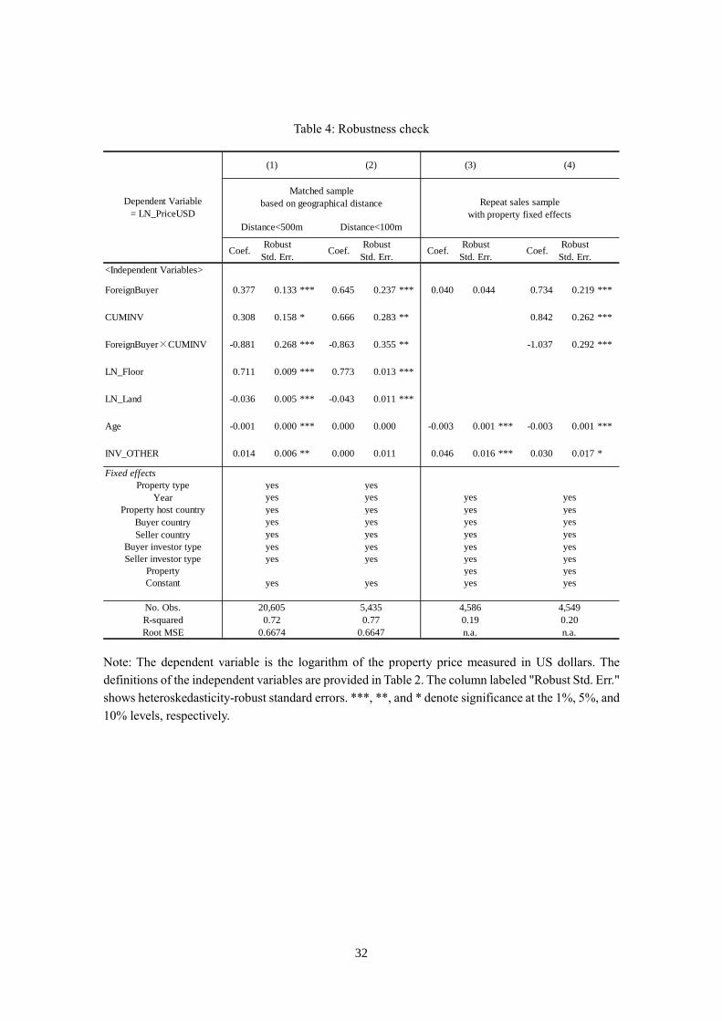
14

The results of the matched sample estimation are presented in columns (1) and (2) of Table

4. The most important coefficients are again those on 𝐹𝑜𝑟𝑒𝑖𝑔𝑛𝐵𝑢𝑦𝑒𝑟𝑖,𝑝,𝑏 , 𝐶𝑈𝑀𝐼𝑁𝑉𝑝,𝑏,𝑡 , and

𝐹𝑜𝑟𝑒𝑖𝑔𝑛𝐵𝑢𝑦𝑒𝑟𝑖,𝑝,𝑏 × 𝐶𝑈𝑀𝐼𝑁𝑉𝑝,𝑏,𝑡. The coefficients on these variables are qualitatively the same as

in the baseline estimation; that is, they are positive and significant for 𝐹𝑜𝑟𝑒𝑖𝑔𝑛𝐵𝑢𝑦𝑒𝑟𝑖,𝑝,𝑏 and

𝐶𝑈𝑀𝐼𝑁𝑉𝑝,𝑏,𝑡 and negative and significant for the interaction term of the two. Somewhat surprisingly,

the coefficient on 𝐹𝑜𝑟𝑒𝑖𝑔𝑛𝐵𝑢𝑦𝑒𝑟𝑖,𝑝,𝑏 is substantially larger in column (2) than in column (1) even

though the matched samples of properties purchased by domestic and foreign buyers are located close

to each other.

Next, taking one step further, we employ the repeat-sales approach in order to more

rigorously control for property fixed effects. Specifically, we identify real estate properties that are

sold multiple times using the latitude and longitude information of each property. We further limit the

sample of such repeat-sales properties to those that were purchased both by a domestic and a foreign

investor at least once during the observation period. We end up with a sample of more than 4,500

properties, which we use for the estimation controlling for property fixed effects. Note that some of

the property characteristics variables, such as LN_Floor and LN_Land, were dropped, since these

variables are time-invariant within the repeat-sales sample.

The results are shown in columns (3) and (4) of Table 4. The coefficients in these estimations

on 𝐹𝑜𝑟𝑒𝑖𝑔𝑛𝐵𝑢𝑦𝑒𝑟𝑖,𝑝,𝑏, 𝐶𝑈𝑀𝐼𝑁𝑉𝑝,𝑏,𝑡, and 𝐹𝑜𝑟𝑒𝑖𝑔𝑛𝐵𝑢𝑦𝑒𝑟𝑖,𝑝,𝑏 × 𝐶𝑈𝑀𝐼𝑁𝑉𝑝,𝑏,𝑡 are qualitatively the

same as those in the baseline estimation. They are positive and significant for 𝐹𝑜𝑟𝑒𝑖𝑔𝑛𝐵𝑢𝑦𝑒𝑟𝑖,𝑝,𝑏

and 𝐶𝑈𝑀𝐼𝑁𝑉𝑝,𝑏,𝑡 and negative and significant for the interaction terms. The only exception is the

coefficient on 𝐹𝑜𝑟𝑒𝑖𝑔𝑛𝐵𝑢𝑦𝑒𝑟𝑖,𝑝,𝑏 in column (3), which is positive but statistically insignificant. This

result implies that, at least in this sample, the unconditional marginal impact associated with

𝐹𝑜𝑟𝑒𝑖𝑔𝑛𝐵𝑢𝑦𝑒𝑟𝑖,𝑝,𝑏 is not statistically different from zero.

To summarize, we control for locational proximity and property-level fixed-effects in a more

rigorous manner than in the baseline so as to correctly identify the impact of purchases by foreign

investors. In both approaches, i.e., when limiting the sample to matched properties in close proximity

and when employing the repeat-sales sample, we find that foreign investors pay significantly higher

prices than domestic investors and that the extent to which foreign investors overpay is smaller the

larger is the cumulative investment from the country of foreign buyers in the host country.6

6 Given that the variable CUMINV might take a value close to one if investors headquartered in country A invest in

country B for the first time, we carry out two robustness checks. The first is to exclude cases in which a country has

15

4.3. Subsample estimations

In this subsection, we examine how the estimation results in Table 3 are affected when we

use different subsamples. First, we split the observation period into two subperiods. The results are

presented in Table 5. The first two columns show the results when we split the period into the period

through 2010 (column (1)) and after 2010 (column (2)), while the next two columns show the results

for the subperiod through 2008 (column (3)) and after 2008 (column (4)). Overall, the coefficients are

qualitatively the same as those in Table 3 with the exception of those in column (3), where all the

coefficients on 𝐹𝑜𝑟𝑒𝑖𝑔𝑛𝐵𝑢𝑦𝑒𝑟𝑖,𝑝,𝑏 , 𝐶𝑈𝑀𝐼𝑁𝑉𝑝,𝑏,𝑡 , and 𝐹𝑜𝑟𝑒𝑖𝑔𝑛𝑏𝑢𝑦𝑒𝑟𝑖,𝑝,𝑏 × 𝐶𝑈𝑀𝐼𝑁𝑉𝑝,𝑏,𝑡 are

statistically insignificant. 7 A notable feature in the results is that the impact associated with

𝐹𝑜𝑟𝑒𝑖𝑔𝑛𝐵𝑢𝑦𝑒𝑟𝑖,𝑝,𝑏 is substantially larger in columns (2) and (4) than in columns (1) and (3). Given

that the later periods were periods when real estate markets were recovering from the global financial

crisis, this result shows that the importance of information asymmetry increased after the financial

crisis. This result somewhat contradicts the widely held view that prices are more likely to be above

fundamentals during boom periods.

Second, we split the sample based on the type of property purchased and present the results

in Table 6. Specifically, we focus on the following five categories: apartments (column (1)), hotels

(column (2)), industrial (column (3)), offices (column (4)), and retail (column (5)). Looking at the

coefficients on 𝐹𝑜𝑟𝑒𝑖𝑔𝑛𝐵𝑢𝑦𝑒𝑟𝑖,𝑝,𝑏, 𝐶𝑈𝑀𝐼𝑁𝑉𝑝,𝑏,𝑡, and 𝐹𝑜𝑟𝑒𝑖𝑔𝑛𝐵𝑢𝑦𝑒𝑟𝑖,𝑝,𝑏 × 𝐶𝑈𝑀𝐼𝑁𝑉𝑝,𝑏,𝑡, we find

that only for industrial and office properties do we obtain qualitatively similar results as in the baseline.

In contrast, for the other types of properties including apartments, the signs on the coefficients of

interest are consistent with our baseline results, but the coefficients are insignificant. The above results

suggest that information asymmetry is more likely to be present in the case of types of property whose

value is more difficult to measure (e.g., properties for business use) than in the case types of properties

whose structures are standardized and whose values are relatively easy to measure (e.g., residential

properties).

exposure to properties in only one country. In the second robustness check, instead of CUMINV, we use the log of the

numerator of CUMINV, that is the cumulative investment from country A in country B (without normalizing by the total

investment from country A). Both estimations provide results consistent with the baseline results. 7 Note that these statistically insignificant coefficients for the period before 2008 may be due to the way CUMINV is

constructed. In order to accurately measure a country’s investment experience, which CUMINV seeks to gauge,

information for a longer period than the subperiod through 2008 may be necessary.

16

4.4. Estimations with additional explanatory variables

In this subsection, we examine how the baseline results in Table 3 change when we introduce

additional variables. In the baseline analysis, we employed dummies for the type of investor

purchasing a property as well as buyer country-year dummies and property host country-year dummies

without specifying the mechanisms how these dummies affect real estate prices. To be more specific

about the mechanisms, we add two sets of variables in Equation (1). The first set concerns the buyer’s

views and objectives regarding the investment: whether the buyer regards the investment as low-risk

and low-return (Core=1) or otherwise (Core=0), the buyer intends to increase the value of the property

and regards the investment as medium-to-high risk and medium-to-high return (ValueAdded=1) or

otherwise (ValueAdded=0), or the buyer intends to occupy the property him/herself (Occ=1) or

otherwise (Occ=0). In our estimation, we drop Occ from the independent variables and include only

Core and ValueAdded to measure the impact associated with Core and ValueAdded, using Occ as the

baseline case.8 The second set of variables measures the buyer’s investment opportunities both in

his/her home country (Buyer_YoY_Return) and in the host country (Host_YoY_Return). Note that the

sample size decreases substantially, since these additional explanatory variables are available only for

a limited number of observations. For example, we employ Buyer_YoY_Return constructed from the

housing price index for a limited number of countries by the Federal Reserve Bank of Dallas.

Table 7 shows the results, which reveal a number of notable findings. First, the signs of the

coefficients on 𝐹𝑜𝑟𝑒𝑖𝑔𝑛𝐵𝑢𝑦𝑒𝑟𝑖,𝑝,𝑏, 𝐶𝑈𝑀𝐼𝑁𝑉𝑝,𝑏,𝑡, and 𝐹𝑜𝑟𝑒𝑖𝑔𝑛𝐵𝑢𝑦𝑒𝑟𝑖,𝑝,𝑏 × 𝐶𝑈𝑀𝐼𝑁𝑉𝑝,𝑏,𝑡 are the

same as those in the baseline results, although the coefficient on 𝐶𝑈𝑀𝐼𝑁𝑉𝑝,𝑏,𝑡 is statistically

insignificant. Second, buyers’ investment objective has a significant impact on the price they pay. It

turns out that buyers that regard their investment as medium-to-high risk and expect medium-to-high

returns end up paying the highest prices. Third, investment opportunities in buyers’ home country, but

not those in the host country, have a significant positive impact on the purchase prices. Buyers whose

home country real estate market is booming may be less likely to be financially constrained and end

up in paying over the odds for real estate overseas.

4.5. Testing for spillover effects

The results presented in Tables 3 to 7 have shown that foreign real estate buyers tend to pay

8 The data contain “Other” as another category regarding buyers’ purchase motive. Since we do not have more precise

information on this category, we drop the observations for which “Other = 1.”

17

higher prices than domestic buyers. Given that this result is obtained controlling for a wide range of

property and investor characteristics, it seems possible that property purchases by foreign investors

might lead to demand pressure in host country real estate markets. However, whether property

purchases by foreign investors at inflated prices create sufficient pressure to have a wider impact on

the local real estate market is an empirical matter. Specifically, it will depend on the number of

investable properties in the local market and hence the elasticity of supply. In addition, if the markets

in which foreign and domestic buyers invest are segmented, the higher prices paid by foreign buyers

will not necessarily generate spillover effects on the wider property market.

Based on these considerations, we focus only on properties bought by domestic investors

and how the prices paid by them are related to the prices of properties nearby purchased by foreign

investors. Properties nearby are those within a 100m radius. In order to identify the causal impact of

property purchases by foreign buyers, we distinguish properties bought by domestic investors into

those bought before and after property purchases by foreign investors nearby. The former properties

are then used as the control group, while the latter are the treatment group. If there are any causal

spillover effects from the higher prices paid by foreign buyers on the prices paid by domestic buyers,

we should see a statistically significant difference in the prices paid by the two different groups of

domestic buyers.

Table 8 outlines the sample we use for this spillover test. Specifically, the table shows that

among the 27,505 properties bought by domestic buyers, 23,406 do not have any properties bought by

foreign investors nearby (i.e., within a radius of 100m).9 The number of properties bought by domestic

investors that do have a property or properties bought by foreign investors nearby is a total of 4,099.

In 1,504 of these case, the domestic investor bought the property before the foreign investor(s), while

in 2,101 cases, the domestic investor bought the property after the foreign investor(s). Meanwhile, in

494 cases, foreign buyers bought properties nearby both before and after the domestic buyer.

Using these 27,505 observations, we run the following estimation, which, in addition to

various control variables, includes the following two dummy variables: 𝑃𝑙𝑎𝑐𝑒𝑏𝑜𝑖,𝑝,𝑏, which takes a

value of one if property i has a property nearby purchased by a foreign buyer after the property was

9 To construct the table and the 1_spillover and 1_placebo variables, we do not set specific upper limits on the length

of time between a purchase by a domestic buyer and a purchase by a foreign buyer. As a robustness check, we implement

an alternative estimation in which the variables are constructed in a more restrictive manner, that is, the variables take

a value of one only in the case there is less than a year between the purchases by domestic and foreign buyers. The

results (not reported) are not substantially different from those in Table 9.

18

bought, and 𝑆𝑝𝑖𝑙𝑙𝑜𝑣𝑒𝑟𝑖,𝑝,𝑏, which takes a value of one if property i has a property nearby purchased

by a foreign buyer before the property was bought. Note that as we focus only on properties bought

by domestic investors, we cannot include 𝐹𝑜𝑟𝑒𝑖𝑔𝑛𝐵𝑢𝑦𝑒𝑟𝑖,𝑝,𝑏 and 𝐶𝑈𝑀𝐼𝑁𝑉𝑝,𝑏,𝑡 in the equation. If

there are any spillover effects as a result of purchases by foreign buyers, we expect 𝛿1 > 0 but 𝛿2=0,

since purchases by foreign buyers after purchases by domestic buyers should not affect the price paid

by domestic buyers. Thus, we estimate the following equation:

𝐿𝑁_𝑃𝑟𝑖𝑐𝑒𝑈𝑆𝐷𝑖,𝑝,𝑏,𝑠,𝑡 = 𝛼 + 𝛿1𝟏_𝑠𝑝𝑖𝑙𝑙𝑜𝑣𝑒𝑟𝑖,𝑝,𝑏 + 𝛿2𝟏_𝑝𝑙𝑎𝑐𝑒𝑏𝑜𝑖,𝑝,𝑏

+𝛿3𝟏_𝑠𝑝𝑖𝑙𝑙𝑜𝑣𝑒𝑟𝑖,𝑝,𝑏 × 1_𝑝𝑙𝑎𝑐𝑒𝑏𝑜𝑖,𝑝,𝑏 + 𝑿𝑖𝑡𝜸

+ 𝜂𝑝1 + 𝜂𝑏

2 + 𝜂𝑠3 + 𝜂𝑡

4 + 휀𝑖,𝑡 (3)

Table 9 presents the estimation results. We find that both 𝛿1 and 𝛿2 are greater than zero,

indicating that domestic buyers tend to pay more for properties that are located close to properties

purchased by foreign buyers than for properties that are not close properties purchased by foreign

buyers. We also find that these coefficients are almost identical. This indicates that there exists no

substantial difference in the premium paid by domestic buyers regardless of whether they purchased

their property before or after the foreign buyer(s) purchased theirs. In sum, these results provide

evidence for a selection effect in that prices are higher for properties purchased by foreign buyers,

while we find no evidence for spillover effects.

5. Conclusion

In this study, we examined whether foreign real estate buyers pay higher prices than their

domestic counterparts and, finding that this is the case, investigate whether this has any spillover

effects in terms of driving up property prices. Using about 30,000 observations covering realty

investment transactions in eight countries and controlling for a comprehensive list of property and

transaction characteristics, we find the following. First, foreign investors pay substantially higher

prices than domestic investors even after taking various controls into account. Second, this price

difference is smaller the larger the cumulative aggregate real estate investment from the buyers’

country in the host country. These results suggest that foreign investors tend to pay over the odds when

they are less informed about local property markets and that the extent to which they overpay decreases

19

with buyers’ investment experience, which, we assume, is represented by the cumulative investment.

Third, despite the finding that foreign investors tend to pay over the odds, we did not find any evidence

of significant spillover effects of foreign real estate investment on local real estate markets. The last

result suggests that the supply of properties in host countries is fairly elastic and/or there is a certain

degree of market segmentation between foreign and domestic property buyers.

Finally, we highlight potential avenues for future research. First, an important extension of

this study is to examine if really no spillover effects can be observed under all circumstances and, if

this is the case, to consider why. Second, another important research direction would be to examine

investors’ choice among multiple investment locations. We believe these potential extensions could

provide further insights for a better understanding of the price implications of international real estate

transactions.

20

References

Aizenman, J., and Y. Jinjarak (2009) “Current Account Patterns and National Real Estate Markets,”

Journal of Urban Economics 66(2): 75-89.

Autor, D., H. Palmer, J. Christopher, and P. A. Pathak (2014) “Housing Market Spillovers: Evidence

from the End of Rent Control in Cambridge, Massachusetts,” Journal of Political Economy

122(3): 661-717.

Badarinza, C., and T. Ramadorai (2015) “Home Away From Home? Foreign Demand and London

House Prices,” mimeo. Available online at:

http://www.bde.es/f/webbde/INF/MenuHorizontal/SobreElBanco/Conferencias/2015/Archivos/

27_1140B_BADARINZA_PAPER.pdf

Bernanke, B. (2005) “The Global Saving Glut and the U.S. Current Account Deficit,” Remarks at the

Homer Jones Lecture, St. Louis, MO.

Coval, J. D., and T. J. Moskowitz (2001) “The Geography of Investment: Informed Trading and Asset

Prices,” Journal of Political Economy 109(4): 811-841.

Favilukis J., D. Kohn, S. Ludvigson, and S. Van Nieuwerburgh (2013) “International Capital Flows

and House Prices: Theory and Evidence,” in E. L. Glaeser and T. Sinai (eds.), Housing and the

Financial Crisis, NBER, Cambridge, MA, Chapter 6.

Ferrero A. (2014) “House Price Booms, Current Account Deficits, and Low Interest Rates,” Journal

of Money, Credit, and Banking 47(S1): 261-293.

Garmaise, M. J., and T. J. Moskowitz (2004) “Confronting Information Asymmetries: Evidence from

Real Estate Markets,” Review of Financial Studies 17(2): 405-437.

Gompers P., A. Kovner, J. Lerner, and D. Scharfstein (2008) “Venture Capital Investment Cycles: The

Impact of Public Markets,” Journal of Financial Economics 87(1): 1-23.

Hochberg, Y., A. Ljungqvist, and Y. Lu (2007) “Whom You Know Matters: Venture Capital Networks

and Investment Performance,” Journal of Finance 62(1): 251-301.

Jordà, Ò., M. Schularick, and A. M. Taylor (2014) “Betting the House,” NBER Working Paper No.

20771.

Justiniano, A., G. Primiceri, and A. Tambalotti (2014) “The Effects of the Saving and Banking Glut

on the U.S. Economy,” Journal of International Economics 92(S1): S52-S67.

Kurlat, P. (2016) “Asset Markets with Heterogeneous Information,” Econometrics 84(1): 33-85.

Kurlat, P., and J. Stroebel (2015) “Testing for Information Asymmetries in Real Estate Markets,”

Review of Financial Studies 28(8): 2429-2461.

Leary, M. T., and M. R. Roberts (2014) “Do Peer Firms Affect Corporate Financial Policy?” Journal

of Finance 69(1): 139-178.

Sorensen M. (2008) “Learning by Investing: Evidence from Venture Capital,” AFA 2008 New Orleans

Meetings Paper.

21

Figures and Tables

Figure 1: Location of properties (purchased by foreign and domestic investors)

(a) Los Angeles and Paris

Note: The figure shows the locations of properties bought by foreign investors (stars) and domestic

investors (dots) in Los Angeles (upper panel) and Paris (lower panel).

22

(b) Toronto and London


investors (dots) in Toronto (upper panel) and London (lower panel).

23

(c) Tokyo and Sydney


investors (dots) in Tokyo (upper panel) and Sydney (lower panel).

24

Figure 2: Marginal effect of ForeignBuyer (baseline)

Note: The figure shows the marginal effect of ForeignBuyer conditional on the level of CUMINV. The

estimated coefficients are taken from Table 3, column (2).

25

Figure 3: Difference between time-variant seller effects and buyer effects:

The cases of equity funds and pension funds

Note: The figure shows the difference between (i) coefficients on time-variant seller investor type

dummies and (ii) coefficients on time-variant buyer investor type dummies. Specifically, the figure

shows the differences for equity funds and pension funds. The estimated coefficients are taken from

Table 3, column (4).

-4.7

-3.7

-2.7

-1.7

-0.7

0.3

1.3

2.3

2005 2006 2007 2008 2009 2010 2011 2012 2013 2014 2015

Seller effects - Buyer effects:

Equity funds vs. Pension funds

Equity Funds Pension Funds

26

Figure 4: Average and standard deviation of

the difference between time-variant seller effects and buyer effects

Note: The figure shows the averages and standard deviations of the differences between (i) coefficients

on time-variant seller investor type dummies and (ii) coefficients on time-variant buyer investor type

dummies. We calculate the differences for all the types of investors. The estimated coefficients are

taken from Table 3, column (4).

27

Table 1: Tabulation of transaction-level data

Panel (a): Property type

Category Freq. Percent Cum.

Apartment 10,352 35.83 35.83

Development Site 50 0.17 36

Hotel 655 2.27 38.27

Industrial 5,537 19.16 57.43

Office 7,021 24.3 81.73

Other 120 0.42 82.15

Retail 4,966 17.19 99.34

Seniors Housing & Care 192 0.66 100

Total 28,893 100

Panel (b): Year

Year Freq. Percent Cum.

2005 1,719 5.95 5.95

2006 2,308 7.99 13.94

2007 2,817 9.75 23.69

2008 1,867 6.46 30.15

2009 1,164 4.03 34.18

2010 1,832 6.34 40.52

2011 2,282 7.9 48.42

2012 3,283 11.36 59.78

2013 3,771 13.05 72.83

2014 4,409 15.26 88.09

2015 3,441 11.91 100

Total 28,893 100

Panel (c): Country of property location

Country Freq. Percent Cum.

Australia 568 1.97 1.97

Canada 393 1.36 3.33

France 180 0.62 3.95

Hong Kong 62 0.21 4.16

Japan 6,162 21.33 25.49

Netherlands 26 0.09 25.58

United Kingdom 274 0.95 26.53

United States 21,228 73.47 100

Total 28,893 100

28

Table 1: Tabulation of transaction-level data (continued from the previous page)

Panel (d): Buyer investor type


Unknown 533 1.84 1.84

Bank 191 0.66 2.51

Cooperative 1 0 2.51

Corporate 1,563 5.41 7.92

Developer/Owner/Operator 16,819 58.21 66.13

Educational 112 0.39 66.52

Equity Funds 1,611 5.58 72.09

Finance 281 0.97 73.07

Government 151 0.52 73.59

High Net Worth 548 1.9 75.49

Insurance 192 0.66 76.15

Investment Manager 1,322 4.58 80.73

Listed Funds 35 0.12 80.85

Non-Traded REIT 389 1.35 82.19

Non-Profit 131 0.45 82.65

Open-Ended Funds 103 0.36 83

Other 23 0.08 83.08

Other/Unknown 2 0.01 83.09

Pension Funds 106 0.37 83.46

REIT 3,613 12.5 95.96

Religious 34 0.12 96.08

REOC 1,066 3.69 99.77

Sovereign Wealth Funds 67 0.23 100

Total 28,893 100

29

Table 1: Tabulation of transaction-level data (continued from the previous page)

Note: The panels show the distribution of property transactions by property type, transaction year,

country of property location, type of buyer and type of seller, all of which we control for in the

empirical analysis using dummy variables. In the empirical analysis, we also include dummies for

the buyer country and seller country as control variables.

Panel (e): Seller investor type


Unknown 710 2.46 2.46

Bank 726 2.51 4.97

CMBS 1 0 4.97

Cooperative 2 0.01 4.98

Corporate 2,040 7.06 12.04

Developer/Owner/Operator 16,813 58.19 70.23

Educational 40 0.14 70.37

Endowment 3 0.01 70.38

Equity Funds 1,395 4.83 75.21

Finance 602 2.08 77.29

Government 157 0.54 77.84

High Net Worth 669 2.32 80.15

Insurance 245 0.85 81

Investment Manager 1,766 6.11 87.11

Listed Funds 36 0.12 87.24

Non Traded REIT 120 0.42 87.65

Non-Profit 113 0.39 88.04

Open-Ended Funds 116 0.4 88.44

Other 13 0.04 88.49

Pension Funds 120 0.42 88.9

REIT 1,723 5.96 94.87

Religious 61 0.21 95.08

REOC 1,400 4.85 99.92

Sovereign Wealth Funds 22 0.08 100

Total 28,893 100

30

Table 2: Summary statistics

Note: The table shows the summary statistics of the variables used in our empirical analysis.

Variable Definition Obs. Mean Std. Dev. Min. Max.

LN_PriceUSDLog of transaction price measured in

USD28893 16.03 1.21 0.00 21.41

CUMINV

Ratio of (i) cumulative investment

amount from buyer country in property

location country until the preceding

month to (ii) the total cumulative

investment of buyer country until the

preceding month

28893 0.78 0.18 0.00 1.00

ForeignBuyer

Dummy variable taking a value of 1 if

buyer country is different from property

location country

28893 0.05 0.21 0 1

LN_Floor Log of floor area measured in square feet 28893 10.54 1.20 -0.87 19.02

LN_Land Log of land size measured in acres 28893 -0.45 1.83 -13.09 13.76

Age

Property age measured as the difference

between the observation year and the

year in which the property was

developed

28893 42.78 31.83 -5 360

Occ


the purpose of the investment is recorded

as "Occupy" (i.e., own use)

28892 0.05 0.22 0 1

ValueAdded



as "Value-Added Investment"

28892 0.19 0.39 0 1

Core



as "Core Investment"

28892 0.45 0.50 0 1

Buyer_YoY_Return

Return measured as the growth rate of the

housing price index in the buyer's country

from 5 quarters prior to the current

period to the quarter preceding the

current period (i.e., 4 quarters = one

year)

28011 0.02 0.05 -0.12 0.19

Host_YoY_Return

Return measured as the growth rate of the

housing price index in the host country

from 5 quarters prior to the current

period to the quarter preceding the

current period (i.e., 4 quarters = one

year), divided by the average of these

returns for all countries

28633 18.59 279.83 -6021 1981

INV_OTHER

Log of investment flows from all

countries other than the buyer country to

property location country during the

current month measured in USD

28893 19.82 0.97 13 23

31

Table 3: Baseline estimation

Note: The dependent variable is the logarithm of the property price measured in US dollars. The

definitions of the independent variables are provided in Table 2. The column labeled "Robust Std. Err."

shows heteroskedasticity-robust standard errors. ***, **, and * denote significance at the 1%, 5%, and

10% levels, respectively.

Coef.Robust

Std. Err.Coef.

Robust

Std. Err.Coef.

Robust

Std. Err.Coef.

Robust

Std. Err.

<Independent Variables>

ForeignBuyer 0.122 0.038 *** 0.409 0.122 *** 0.110 0.038 *** 0.163 0.042 ***

CUMINV 0.325 0.145 **

ForeignBuyer×CUMINV -0.798 0.260 *** -0.835 0.246 ***

LN_Floor 0.701 0.007 *** 0.701 0.007 *** 0.697 0.007 *** 0.696 0.008 ***

LN_Land -0.040 0.004 *** -0.040 0.004 *** -0.036 0.004 *** -0.037 0.004 ***

Age -0.001 0.000 *** -0.001 0.000 *** -0.001 0.000 *** -0.001 0.000 ***

INV_OTHER 0.016 0.005 *** 0.014 0.005 ***

Fixed effects

Property type

Year

Property host country

Buyer country

Seller country

Buyer investor type

Seller investor type

Property type×Year

Property host country×Year

Buyer country×Year

Seller country×Year

Buyer investor type×Year

Seller investor type×Year

Constant

No. Obs.

R-squared

Root MSE

yes yes

yes yes

yes yes

yes yes

yes yes

yes yes

yes yes

yes yes

28,934 28,893 29,397 29,090

yes yes

0.6623 0.6621 0.6389 0.6393

0.70 0.70 0.73 0.73

yes yes yes yes

yes yes

yes yes

yes yes

yes yes

Dependent Variable

= LN_PriceUSD

(1) (2) (3) (4)

32

Table 4: Robustness check





Coef.Robust

Std. Err.Coef.

Robust

Std. Err.Coef.

Robust

Std. Err.Coef.

Robust

Std. Err.


ForeignBuyer 0.377 0.133 *** 0.645 0.237 *** 0.040 0.044 0.734 0.219 ***

CUMINV 0.308 0.158 * 0.666 0.283 ** 0.842 0.262 ***

ForeignBuyer×CUMINV -0.881 0.268 *** -0.863 0.355 ** -1.037 0.292 ***

LN_Floor 0.711 0.009 *** 0.773 0.013 ***

LN_Land -0.036 0.005 *** -0.043 0.011 ***

Age -0.001 0.000 *** 0.000 0.000 -0.003 0.001 *** -0.003 0.001 ***

INV_OTHER 0.014 0.006 ** 0.000 0.011 0.046 0.016 *** 0.030 0.017 *

Fixed effects

Property type

Year


Buyer country

Seller country

Buyer investor type


Property

Constant

No. Obs.

R-squared

Root MSE

yes yes yes yes

yes yes

yes yes yes yes

yes yes yes yes

yes yes yes yes

yes yes

yes yes yes yes

yes yes

0.6674 0.6647 n.a. n.a.

0.72 0.77 0.19 0.20

yes yes

20,605 5,435 4,586 4,549

yes yes yes yes

Dependent Variable

= LN_PriceUSD

(4)(1) (2) (3)

Matched sample

based on geographical distance Repeat sales sample

with property fixed effects

Distance<500m Distance<100m

33

Table 5: Estimation for different observation periods





Coef.Robust

Std. Err.Coef.

Robust

Std. Err.Coef.

Robust

Std. Err.Coef.

Robust

Std. Err.


ForeignBuyer 0.449 0.161 *** 1.478 0.353 *** 0.026 0.176 1.418 0.290 ***

CUMINV 0.346 0.187 * 1.750 0.434 *** -0.126 0.207 1.525 0.353 ***

ForeignBuyer×CUMINV -1.190 0.370 *** -1.163 0.489 ** -0.442 0.348 -2.201 0.477 ***

LN_Floor 0.720 0.010 *** 0.694 0.010 *** 0.745 0.011 *** 0.688 0.009 ***

LN_Land -0.039 0.007 *** -0.040 0.005 *** -0.049 0.009 *** -0.039 0.005 ***

Age -0.003 0.000 *** 0.000 0.000 -0.003 0.000 *** 0.000 0.000

INV_OTHERS 0.017 0.009 * 0.005 0.007 0.022 0.011 ** 0.007 0.006

<Fixed-effect>

Property type

Year


Buyer country

Seller country

Buyer investor type


Constant

No. Obs.

R-squared

Root MSE

Dependent var

= LN_PriceUSDYear<=2010 Year>=2011 Year<=2008 Year>=2009

(1) (2) (3) (4)

yes yes yes yes

yes yes yes yes

yes yes yes yes

yes yes yes yes

yes yes yes yes

yes yes yes yes

yes yes yes yes

yes yes yes yes

11,707 17,186 8,711 20,182

0.73 0.70 0.75 0.69

0.6259 0.6715 0.5940 0.6799

34

Table 6: Estimation for different property types





Coef.Robust

Std. Err.Coef.

Robust

Std. Err.Coef.

Robust

Std. Err.Coef.

Robust

Std. Err.Coef.

Robust

Std. Err.


ForeignBuyer 0.274 0.283 2.867 1.539 * 0.506 0.180 *** 0.849 0.219 *** 0.465 0.497

CUMINV 0.114 0.322 2.835 1.912 0.490 0.221 ** 1.023 0.256 *** 0.231 0.628

ForeignBuyer×CUMINV -1.191 1.147 -2.961 2.312 -4.071 0.737 *** -0.865 0.322 *** -0.107 0.982

LN_Floor 0.690 0.019 *** 0.771 0.039 *** 0.562 0.013 *** 0.853 0.011 *** 0.584 0.015 ***

LN_Land 0.018 0.008 ** -0.047 0.029 -0.016 0.007 ** -0.065 0.008 *** -0.033 0.009 ***

Age -0.005 0.000 *** 0.001 0.001 0.003 0.000 *** 0.000 0.000 0.000 0.000

INV_OTHERS 0.007 0.008 0.041 0.046 0.010 0.012 0.018 0.010 * 0.003 0.015

<Fixed-effect>

Year


Buyer country

Seller country

Buyer investor type


Constant

No. Obs.

R-squared

Root MSE

0.77

0.6554

yes

yes

7,021

yes

0.6044

0.76

0.6618

Office

yes

yes

yes

yes

yes

yes

yesyes

655

0.60

5,537

Hotel

yes

yes

yes

Industrial

yes

yes

yes

yes yes

0.65

0.5652

10,352

yes

yes

yes

yes

yes

yes

yes

Apartment

yes

Dependent var

= LN_PriceUSDRetail

yes

yes

yesyes

(1) (2) (3) (4) (5)

yes

0.66

0.6977

yes

yes

1,966

yes

35

Table 7: Additional independent variables





Dependent var

= LN_PriceUSDCoef.

Robust

Std. Err.


ForeignBuyer 0.291 0.142 **

CUMINV 0.168 0.154

ForeignBuyer×CUMINV -1.786 0.590 ***

LN_Floor 0.715 0.010 ***

LN_Land -0.051 0.005 ***

Age -0.001 0.000 ***

INV_OTHERS -0.003 0.007

ValueAdded 0.116 0.037 ***

Core 0.055 0.034

Buyer_YoY_Return 1.836 0.218 ***

Host_YoY_Return 0.000 0.000

<Fixed-effect>

Property type yes

Year yes

Property host country yes

Seller country yes

Buyer investor type yes

Seller investor type yes

Constant yes

No. Obs. 19,276

R-squared 0.70

Root MSE 0.6771

36

Table 8: Sample for spillover test

Note: The table lists the number of transacted properties by domestic buyers. Among the 27,505

properties bought by domestic buyers, 23,406 do not have any properties bought by foreign investors

nearby (i.e., within a radius of 100m). The number of properties bought by domestic investors that do

have a property or properties bought by foreign investors nearby is a total of 4,099. In 1,504 of these

case, the domestic investor bought the property before the foreign investor(s), while in 2,101 cases,

the domestic investor bought the property after the foreign investor(s). Meanwhile, in 494 cases,

foreign buyers bought properties nearby both before and after the domestic buyer.

0 1 Total

0 23,406 1,504 24,910

1 2,101 494 2,595

Total 25,507 1,998 27,505

(b)

1(if distance<100m)_placebo

(a)

1(if distance<100m)_spillover

37

Table 9: Spillover test


definitions of the independent variables are provided in main text. The column labeled "Robust Std.

Err." shows heteroskedasticity-robust standard errors. ***, **, and * denote significance at the 1%,

5%, and 10% levels, respectively.

Dependent var

= LN_PriceUSDCoef.

Robust

Std. Err.


1_spillover 0.189 0.016 ***

1_placebo 0.186 0.018 ***

1_spillover×1_placebo 0.038 0.038

LN_Floor 0.693 0.008 ***

LN_Land -0.046 0.004 ***

Age -0.002 0.000 ***

INV_OTHERS 0.018 0.006 ***

<Fixed-effect>

Property type

Year


Seller country

Buyer investor type


Constant

No. Obs.

R-squared

Root MSE

27,505

0.68

0.6637

yes

yes

yes

yes

yes

yes

yes

geography and realty prices: evidence from …we thank bob white, jim sempere, yiqin wang, doug...

Documents