geog 141 migration(feb07) - university of california, …carr/geog141/geog 141_migrati… · ·...
TRANSCRIPT

Today’s Objectives
• Migration–Definitions–Models–Demographics–Summaries–Case Studies
Population Geography Class 3.1
Human Migration
Population Change = Fertility + Mortality + Migration
MIGRATION
• More complex than birth and death
• No limits (unlike fertility and mortality)
• Migration has two regions (origin & destination)

What is migration?

What is migration?
• Move across town?• Students move to university each year?
• Key variables – Space, distance, time, frequency

Migration Defined

Migration Defined
• Permanent change in residence • Migrants cross some political boundary
– duration of stay usually > 1 year– total displacement of community affiliation
• jobs, church, school…
• “mover” defined as in moving within a city– no crossing of political boundaries & only partial
displacement of community affiliation

Examples
• Urban commuter: local, recurrent, no change in residence (may cross political boundaries – SB –Goleta)
• Student or “migrant” far worker: not local, recurrent no complete change of community affiliation
• “Circulation”: recurrent movement – Examples: SB-Goleta = migration
• move across town ≠ migration

Basic concepts/measures
• Gross migration– [(people in + people out)/mid year population)]*1000
• Net migration: – [(#incoming - # outgoing)/mid year population)]*1000
• In-migration:– called “in-migration” within a country; “immigration” for those
entering a country– (# immigrants/ mid year population of destination)*1000
• Out-migration: “emigration” for those leaving a country; “out migration” within country – # emigrants/mid-year population of origin

Estimation Techniques
• For unavailable data
• Residuals Method: estimates “crude” net rate– net migrationt=1-2 = (Pt=2-Pt=1) – (Bt=1-2 -Dt=1-2)– Population change in interval, minus natural increase
• Surviving cohort method:– using life tables; age-specific survival rates can be
obtained for the age class in question

Migration Theories
• Ravenstein• Lee (Push-Pull)• Gravity Model• Intervening Opportunity Model• Chain Migration

Ravenstein
1st “Laws of Migration” 1870s-80s• Distance: most short (local rural to urban) longer
distances to larger cities• Gender: females mostly short migration
(marriage/mills) males more common longer• Technology: as transport improves leads to
greater volume of migration• Motive: economic motives main justification• Residence: rural residents more likely to be
migrants

Patterns of migrants noted by Ravenstein
• Stream: migrants from a given rural area often make up a stream from some origin to same destination– also a counter-stream of returnees
• Steps: migrants more rural therefore local/small town then small town to major town (not directly rural to big city)
Lee’s Push-Pull Model(1940s)
An attempt to explain the patterns of migration
• Migration was a decision (individual or family) therefore depends on:– characteristics of the origins– characteristics of the destination– nature of intervening obstacles (e.g. cost,
borders, …)– nature of the people

Lee’s Push-Pull Model
Lee’s Push-Pull Model• Push/pulls can vary widely – economic is probably most
important– But also climate; quality of school, nearness to family,
etc.
• A potential migrant takes into consideration a balance of the +’s and –‘s of origin + destination along with difficulty of intervening obstacles in deciding whether or not to migrate

Constraints: Lee’s Behavioral Model
• Lee’s Push-Pull Model does not account for the fact that some people have less ability to act on migration decisions
• Lee only looks at people’s desire to act according to their assessment or desirability
• People differ in their ability to act/migrate (no matter how desirable migration may seem)– e.g. poor people may not be able to migrate

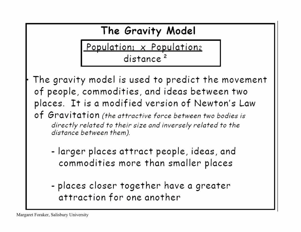
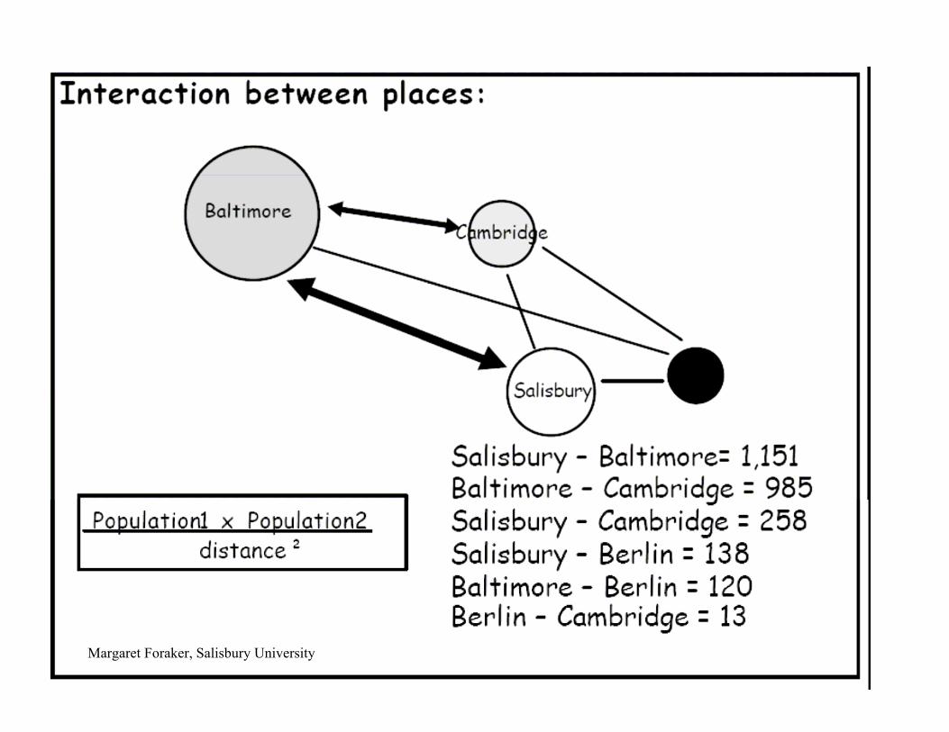
Gravity Model• Uses population of origin and destination as
measures of diversity• Distance a major obstacle• Model empirically adjusted to account for special
circumstances• Very simplistic model:
– does not account for other factors re: the O + D– assumes distance = obstacle i.e. cost
• Attraction may be economic; obstacle may not be distance (e.g. borders)
Margaret Foraker, Salisbury University
Margaret Foraker, Salisbury University

Intervening Opportunity Model
• Migrants are open to possible opportunities that may lie between origin and destination
• Example of “step” migration rural → urban (goal is job/city life)– migrant might stop in local town instead of going all
the way to major city if he/she gets a job…– later, that resident might move to large city in search of
opportunities– therefore a typical process is rural to small city to major
city (except if major city dominates a country)

CHAIN MIGRATION
• Opportunities localized within cities• Migrants use established transport routes or
streams– flow of information about a destination back to origins
• Follows migrants path therefore → ↑ knowledge of destination (↓ obstacle ↑ attractiveness)
• Previous migrant helps later people follow this stream flow (e.g. international migration to the U.S. – (Mexico/Santa Barbara; Quebec/Lewiston, ME)

Counter Stream Migration
• When migrant finds destination not as attractive as imagined
• Usually smaller – except if origin and destination are similar

Summary• Ravenstein’s observations about migration +
migrants– distance; gender; technology; motive; residence– stream; steps
• Lee’s Push-Pull Model: decision-making– characteristics of origin, destination, obstacles,
migrants – role of diversity and perception– problem of constraints
• Gravity Model → goal to predict volume• Intervening Obstacle Model (better describe
patterns)• Chain Migration

Demographic CharacteristicsWho Migrates?

Demographic CharacteristicsAge
• Young adults: 2/3 of people in 20s in last 5 years! – 1/3 move to another county; 1/6 to another state– leave parental home for job, marriage– have few major ties to origin– little attachment to preexisting job– in good health– little major accumulation of stuff– females slightly younger than males
• Relatively little movement of retirement aged individuals

Demographic CharacteristicsGender
• High rural-urban migration in developing world now
• High migration to USA, Europe, rich Middle Eastern nations
• Majority of international migration is male– longer distances especially

Demographic CharacteristicsMarital Status
• Divorced move most in USA – desire for “new” start -- fewer ties?
• Many migrants are young families and this may be especially true for long-distance international migration

Demographic CharacteristicsSocioeconomic Characteristics
• Education: those with more formal education more likely to migrate– US college grads 2x more likely than HS drop
out– Developing world rural → urban migration:
those that migrate have more formal education– Increased education →↑ knowledge of
possibilities at a distance

Demographic CharacteristicsMigrant Occupations
• Unskilled have usually widely available local jobs so move is less necessary or shorter-- less change
• Unskilled probably have less $ therefore obstacles are larger
• Professionals such as MDs, dentists, vets, lawyers in private practices are less mobile since its hard to set up a new practice
• In US, most migrants move for a new job

Demographic CharacteristicsMigrant Ethnicities
• African-Americans in USA 1940-1970– 4.3 million African-Americans left “the South”
• Mostly rural to urban migration • Well developed streams and chain
migration – voluntary “Pull” but also “Push” as
mechanization increases after Depression

Demographic CharacteristicsPlace Characteristics
• environmental attractions • economic attractiveness • social issues attraction
– schools, crime, pollution, crowding, cost of living

Place Characteristics (cont.)Place vs. Migrant Values
• Lifestyle preference for less crowding; more “nature”– metro areas have serious negatives (pushes)– ↑crime; pollution; crowding/traffic; high costs; ↓
schools– Rural-semi suburban has +/- opposite “Pulls”– Firms move out of city also for similar reason

Political-Economy
• Argues that the behavioral approach of Lee (et. al) only deals with part of the issue
• Migration is a human response that occurs when different modes of production/economy interact– especially wage labor/capitalist

Political-Economy (cont.)
• Familial mode vs. wage labor mode to explore how it affected fertility
• Theory holds that when capitalist modes or production appear; it dislocates traditional familial modes and migration is a consequence
• Capitalist factory will be located in place of most profit
• Labor has historically been seen as the movable factor of production

•This argument can help explain how “late capitalism’s” restructuring affects migration
•Some restructuring → movement of factories etc. to low wage areas outside a country
•Marxist: core-periphery
Political-Economy (cont.)

Zelinsky’s Migration Transition
• Four States of Transition

Zelinsky’s Migration Transition
• Pre-Modern– small in volume but lots of circulation type movements– Rural to rural migration dominates
• Transitional (LDCs now in varying stages)– Rural to Urban migration dominates: Urban Pull (jobs) &
Rural Push– ↑ transportation tech. ↓ cost of long distance movement

Zelinsky’s Migration Transition• Post-Transitional: “advanced societies”
– ↑ circulation for leisure (summer homes etc.)– Rural → urban transition finished – International Labor Migration from LDCs to
MDCs – High rate of International urban → urban (job
relocation)
• Future “post industrial” (Is the Future here?)– communications technology may reduce need to
migrate – “Rebound” of Urban → Rural migration
USA Immigration History• Four Major Waves

Source: Immigration and Naturalization Service, 1998 Statistical Yearbook
Regional Origins of Immigrants to the United States, Selected Years
Source: Immigration and Naturalization Service, 1998 Statistical Yearbook

USA Immigration History 1st Wave: Pre-Revolution to 1820
• High cost to migration ~ 6 month wages for passage. ~1/3 came as indentured servants/artisans (5+ years to work off)
• Law + Policy (type of barrier)– +/- laissez-faire– Naturalization Act of 1790
• 1808 Congress bans importation of slaves

USA Immigration History 1st Wave: Pre-Revolution to 1820
• Overall migration: ~ 10,000/year in 18th century or fewer
• > 100,000 German Protestants and 250,00 Scotch-Irish Protestants from N. Ireland
• English pulled by promise of better land: 60% of population 1790
• > 600,000 Africans before 1808 (mostly Caribbean)

USA Immigration History 2nd Wave: 1820-1870
• ↑ population in W Europe as Dem.Trans. begins• Population characteristics
– 1820-1860 ~ >5 million; 40% Irish; 1/3 German Catholic; rest British
– Irish Potato Famine + 1848 German Revolution• large % Catholic (by 1860, USA 10% Catholic)• large % end up in cities
• Law + Policy: strong anti-immigrant reactions 1840s-50s but no explicit laws against migration

USA Immigration History 3rd Wave: 1870-1940
• 1850-80s European political turmoil = push– population increase due to DT continues
• Huge increase in volume– 1880 = ~ 800,000/year– 1910 > 1,000,000/year

USA Immigration History 3rd Wave: 1870-1940 (cont.)
• Origins Change– 1860-1900 NW Europe ~ 70% (German, Irish, UK, Scandinavia)
& SE Europe ~ 20% (Italy, Spain, Slavs, Jews)– 1900-1920 N+W Europe ~40%, S+E Europe ~40%
• S+E Europeans = Italians, Slavs, Jews– S. Italy ~3.8m 1899-1924– E.Europe (Poles, Russians, Czechs, Ukrainians…)– E. European Jews ~ 1.8m
• Impact– by 1900 most to industrial cities; NE– By 1920s immigrants ~ 15% of US population and
~25% of work force in industrial cities

USA Immigration History 3rd Wave: 1870-1940 (cont.)
• Laws/policies: Qualitative– Immigration Act of 1882: barred “undesirables”and immigration from China (1907 Japan)– 1897-1917 → immigrant test for reading– total migrant limit of 358,000 (1921)
USA Immigration History 3rd Wave: 1870-1940 (cont.)
• Laws/policies: Qualitative– Immigration Act of 1882: barred “undesirables”and immigration from China (1907 Japan)– 1897-1917 → immigrant test for reading– total migrant limit of 358,000 (1921)
• Laws/policies: Quantitative– 1921 National Origins “Quota” Act– 250,000 Jews fled Hitler; most barred because of E.
European origin

USA Immigration History 4th Wave 1940 - Present
• Numeric patterns of legal immigrants 1940s →– very small number in 1930s → 1952– steady increase 1953 → current levels ~ 800,000/year– 2000 census → foreign born 31m → 10% of total
population– net migration ~ 1/3rd of annual population growth in US– Increase in foreign born during 1990s

USA Immigration History 4th Wave 1940 - Present
• Origins– 1900-1920 Europeans ~85%– after 1920s proportions changed (NW Europe
~ 40%, Europe ~ 20%, Latin America ~ 20%, Canada ~ 20%)
– 1960s increase in Latin American fraction (~ 40%)• NW +SE Europe ~ 35%, Asian ~ 13%,
Canada ~12%

USA Immigration History 4th Wave 1940 - Present
• Origins
– 1970s, 1980s• Europe steadily decreasing to ~ 10%• Asian origin increasing to ~50%• Latin America ~ 40% legal – post Vietnam
– 1990s• Latin American migration dominates:
nearly 50% of total (legal)
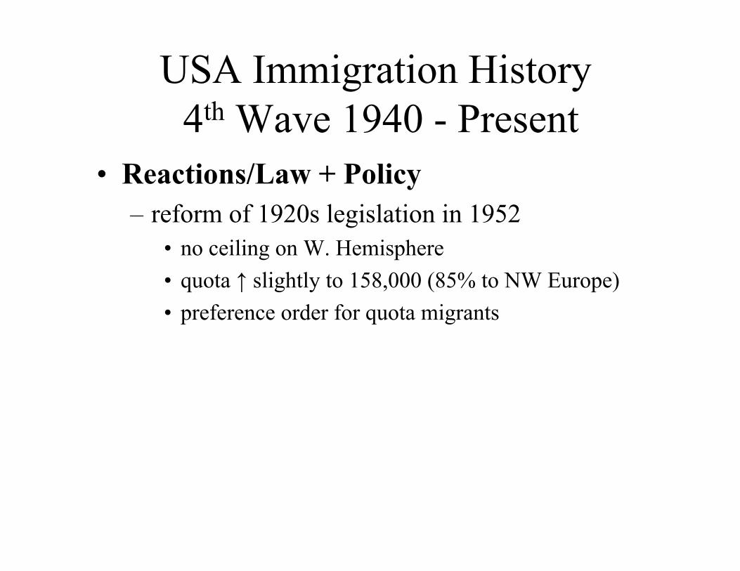
USA Immigration History 4th Wave 1940 - Present
• Reactions/Law + Policy– reform of 1920s legislation in 1952
• no ceiling on W. Hemisphere• quota ↑ slightly to 158,000 (85% to NW Europe)• preference order for quota migrants

USA Immigration History 4th Wave 1940 - Present
• Immigration Act of 1965– eliminated country of origin qualification –– preference for families (1st) and skills (2nd)
• numerical ceiling ~ 170,000 (actual # larger due to families) for E. Hemisphere & 120,000 W. Hemisphere Immigration Reform & Control Act of 1986
• employer sanctions for knowingly hiring illegals• illegally entered before 1982 + resident could get amnesty +
permanent resident status• Ag. Workers can get resident status
• Current political positions

Contemporary International Migration
*%$%#$!!!

Developing World MigrationCauses
• Uneven development-economic, health, education, etc.
• Loosening of traditional social constraints • Rapid population growth • Political and economic marginalization• Environmental Degradation• Strife/war/persecution

Developing World MigrationThree flows: Individual determinants• Rural (virtually all: Rural-rural)
– Increasingly smaller % of migrants– Tend to be most destitute and marginalized
• Urban (both rural-urban and urban-urban)– High % of all migrants– Leaving farm work for urban industrial & service jobs– Tend to be better educated, wealthier than avg. in origin
• International– High % of all migrants– Leave low wages for high wages– Higher educated than avg. in origin area– Males dominate

Developing World Migration
• Rural-Rural Impacts (Guatemala emphasis)– Declining % but great ecological impact– Cause of perhaps most of all global deforestation– Perhaps improves food security and– Relieves population pressures (temporarily) but…– Continues marginalization of poor rural
populations

Developing World Migration
Rural-Urban Impacts– accounts for 1/3 – ½ of growth in cities in
third world • overstretched city services • poor housing; water; sanitary; education;
transportation…– Receive
• “Brain Drain” arrivals • Abundant labor for industry

International Migration Impacts(Case of Mexico coming up later)
• Origin area– Demographic/Economic: Labor
(shortages, loss of labor at key times)–Socio-economic: (“Brain Drain” of
best and brightest)–Environmental: consumption
patterns & land use change

International Migration ImpactsOrigin Area
Remittances - $ sent back to origin by migrants

International Migration Impacts on Destination Area
Social Impacts• Socio-cultural integration: low education
levels; language – little need to use English in S. Texas or S.
California• Increase diversity of local culture

International Migration Impacts on Destination AreaEconomic Impacts
• Labor Market – highly debated and equivocal– Most impacted are those in low-skill jobs– Yet little evidence that on average, immigrants
depress average wages significantly• “Brain Drain”

International Migration Impacts on Destination Area
Public Services (US example)• Schools, health, and other public services, but…• Immigrants pay more taxes than cost in public
services – However, bulk of taxes are paid to Federal
Government while most of public services are mostly state or local government expenditures

International Migration Impacts on Destination Area
Public Services (US example)• Welfare – mostly not eligible for 5 years• Schools
– TFR difference– language difference
International Migration Impacts on Destination Area
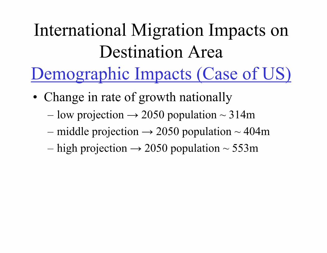
Demographic Impacts (Case of US)• Change in rate of growth nationally
– low projection → 2050 population ~ 314m– middle projection → 2050 population ~ 404m– high projection → 2050 population ~ 553m

International Migration Impacts on Destination Area
Demographic Impacts (Case of US)
• Change in ethnic composition of population– 2000 census → foreign born 31m → 11% of total
population– Increase in foreign born during 1990s

Demographic Impacts (Cont.)
• Current US population includes (2004)– 66% white/non-Hispanic– 4% Asian – 14.1% Hispanic– 13% Afro-American

Demographic Impacts (Cont.)
• Population projections for 2050– 53% white (non-Hispanic)– 14% Afro-American– 24% Hispanic– 8% Asian
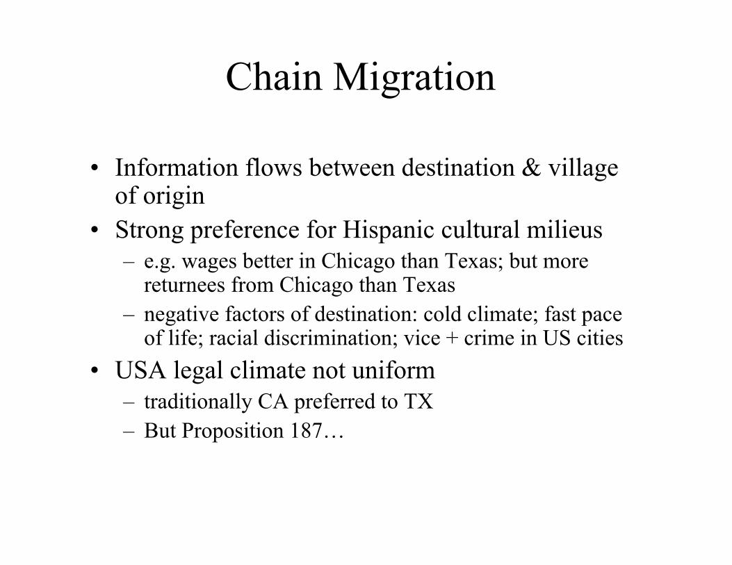
Chain Migration
• Information flows between destination & village of origin
• Strong preference for Hispanic cultural milieus– e.g. wages better in Chicago than Texas; but more
returnees from Chicago than Texas– negative factors of destination: cold climate; fast pace
of life; racial discrimination; vice + crime in US cities• USA legal climate not uniform
– traditionally CA preferred to TX – But Proposition 187…

Migrant’s Characteristics
• Most not permanent: majority return ~1 year• Predominately motivated by Push factors • Predominately economic motives: few jobs in Mexico; • Individual migrant
– younger than USA (17-24 years old)– more male (but increasing % female)– less well educated– more likely to be married (ages 25-64) ~75%– earn less

•Special Case: Refugees
http://mondediplo.com/maps/forcedtoemigrate
2001

Figure 3: Annual net international migration totals and migration rates in the world's major areas, 1990-1995
•Voluntary: International labor migration (legal and illegal)

http://www.iom.int/DOCUMENTS/OFFICIALTXT/EN/UNPD_Presentation.pd

http://www.iom.int/DOCUMENTS/OFFICIALTXT/EN/UNPD_Presentation.pdf 2000
Area
Percent of total
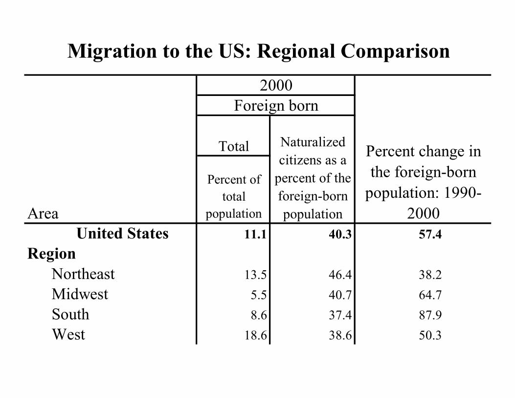
populationUnited States 11.1 40.3 57.4
RegionNortheast 13.5 46.4 38.2Midwest 5.5 40.7 64.7South 8.6 37.4 87.9West 18.6 38.6 50.3
Percent change in the foreign-born
population: 1990-2000
Total
2000Foreign born
Naturalized citizens as a
percent of the foreign-born population
Migration to the US: Regional Comparison

Area
Percent of total
populationState
California 26.2 39.2 37.2New York 20.4 46.1 35.6New Jersey 17.5 46.2 52.7Hawaii 17.5 60.1 30.4Florida 16.7 45.2 60.6Nevada 15.8 36.9 202.0Texas 13.9 31.5 90.2Dist. of Columbia 12.9 30.0 24.9Arizona 12.8 29.6 135.9Illinois 12.3 39.5 60.6Massachusetts 12.2 43.7 34.7Rhode Island 11.4 47.1 25.4Connecticut 10.9 48.7 32.4Washington 10.4 41.9 90.7
Percent change in the foreign-born
population: 1990-2000
Total
2000Foreign born
Naturalized citizens as a
percent of the foreign-born population
Migration to the US: State Comparison

Area
Percent of total
populationState
North Carolina 5.3 26.2 273.7Georgia 7.1 29.3 233.4Nevada 15.8 36.9 202.0Arkansas 2.8 29.9 196.3Utah 7.1 30.4 170.8Tennessee 2.8 33.4 169.0Nebraska 4.4 32.0 164.7Colorado 8.6 31.6 159.7Arizona 12.8 29.6 135.9Kentucky 2.0 34.3 135.3South Carolina 2.9 37.1 132.1Minnesota 5.3 37.4 130.4Idaho 5.0 33.1 121.7Kansas 5.0 33.2 114.4Iowa 3.1 32.9 110.3Oregon 8.5 33.6 108.0Alabama 2.0 36.7 101.6Delaware 5.7 42.4 101.6Oklahoma 3.8 34.7 101.2
Percent change in the foreign-born
population: 1990-2000
Total
2000Foreign born
Naturalized citizens as a
percent of the foreign-born population
Migration to the US: State Comparison

Table 1.Ten Places of 100,000 or More Population With the Highest Percentage Foreign-Born: 2000 1
Place and state Total population NumberPercent of total
population
90 percent confidence interval
on percentageUnited States 281,421,906 31,107,889 11.1 11.09 - 11.11
Hialeah, Florida 226,419 163,256 72.1 71.5 - 72.7Miami, Florida 362,470 215,739 59.5 59.0 - 60.0Glendale, California 194,973 106,119 54.4 53.7 - 55.1Santa Ana, California 337,977 179,933 53.2 52.8 - 53.8Daly City, California 103,621 54,213 52.3 51.4 - 53.2El Monte, California 115,965 59,589 51.4 50.5 - 52.3East Los Angeles, California 2 124,283 60,605 48.8 48.0 - 49.6Elizabeth, New Jersey 120,568 52,975 43.9 43.0 - 44.8Garden Grove, California 165,196 71,351 43.2 42.5 - 43.9Los Angeles, California 3,694,820 1,512,720 40.9 40.7 - 41.1
(Data based on sample. For information on confidentiality protection, nonsampling error, sampling error, and definitions, see www.census.gov/prod/cen2000/doc/sf3.pdf)
Foreign born
Migration to the US: County Comparison

Mexican Migration

http://www.ancestry.com/search/rectype/reference/maps/freeimages.asp?ImageID=369
Mexico 1821-1857
Mexico has lost ~ ½ its national territory to the USA since 1824

•Large-scale movement of Mexicans to US starting in 1880s
•Large increase of migration: 1910-1920
Mexico Migration History
• WWI → northward migration to USA• 1920s a period of anti-immigration and violence in
USA• Depression years in USA → return stream• WWII → labor need at even wider scale than WWI• Bracero Program 1942• End of Bracero Program in 1964

•Currently >103 million people
•Urban population ~ 74%
•Urban growth ~ 3%/year
•Major problem with under-employment
•Much migration in Mexico → USA has been circulatory (temporary migration)
•Also permanent migration and daily job commuting in border cities
Mexico

Mexico Migration Spatial Patterns
• Origins in Mexico:– Jalisco, Michoacan, Zacatecas, Guanajuato, & Chihuahua
+ Coahuila (each > 5%)
• Destination in USA:– Texas, California, Illinois, (each > 5%), also New York,
New Jersey, New Mexico, Arizona, Colorado, Oregon, Washington, Florida

Mexico Migration Spatial Patterns
• Patterns of flow “channelization” 2 big flows– Eastern from Coahuila, Nuevo Leon, Tamaulipis, S.L.
Potosi → Texas – Western from Sinaloa, Jalisco, Nayarit, Colima →
California (AZ)• Factors influencing this pattern
– Transportation links with Mexico – Labor contracting patterns: initially RR labor and Ag– Networks of “Coyotes” concentrated in Texas and
California

Bracero Program
• Purpose - to provide legal agricultural labor to Mexicans– Ended in 1964– Not intended as legal migration
• most came, worked, and returned
– 400,000/year in Bracero Program versus 60-70,000 Mexican migrants

End of Bracero Program
• Hundreds of thousands with experience of labor in USA
• Good contacts for jobs etc.• Hundreds of thousands of Mexican families
suddenly deprived of major income source

Border Industrialization Program
Purpose - To increase jobs lost from BraceroProgram
• Maquiladoras: USA, Japanese, Korean industrial firms with plants
• 1990s - 1,000s of plants employing 100,000’s• Border Towns increase growth > 6%/year• Change w/ NAFTA