genetic programming - ucl · 7. genetic programming 187 of gp in section 6. this is followed by a...
TRANSCRIPT
7. Genetic Programming
Genetic Programming
William B. Langdon, Robert I. McKay and Lee Spector
Abstract Welcome to genetic programming, where the forces of nature are used toautomatically evolve computer programs. We give a flavour of where GP has beensuccessfully applied (it is far too wide an area to cover everything) and interestingcurrent and future research but start with a tutorial of how to get started and finishwith common pitfalls to avoid.
1 Introduction
Getting computers to automatically solve problems is central to artificial intelli-gence, machine learning and the broad area covered by what Turing called “machineintelligence” [113]. As we shall show, this is what genetic programming is actuallydoing. Today.
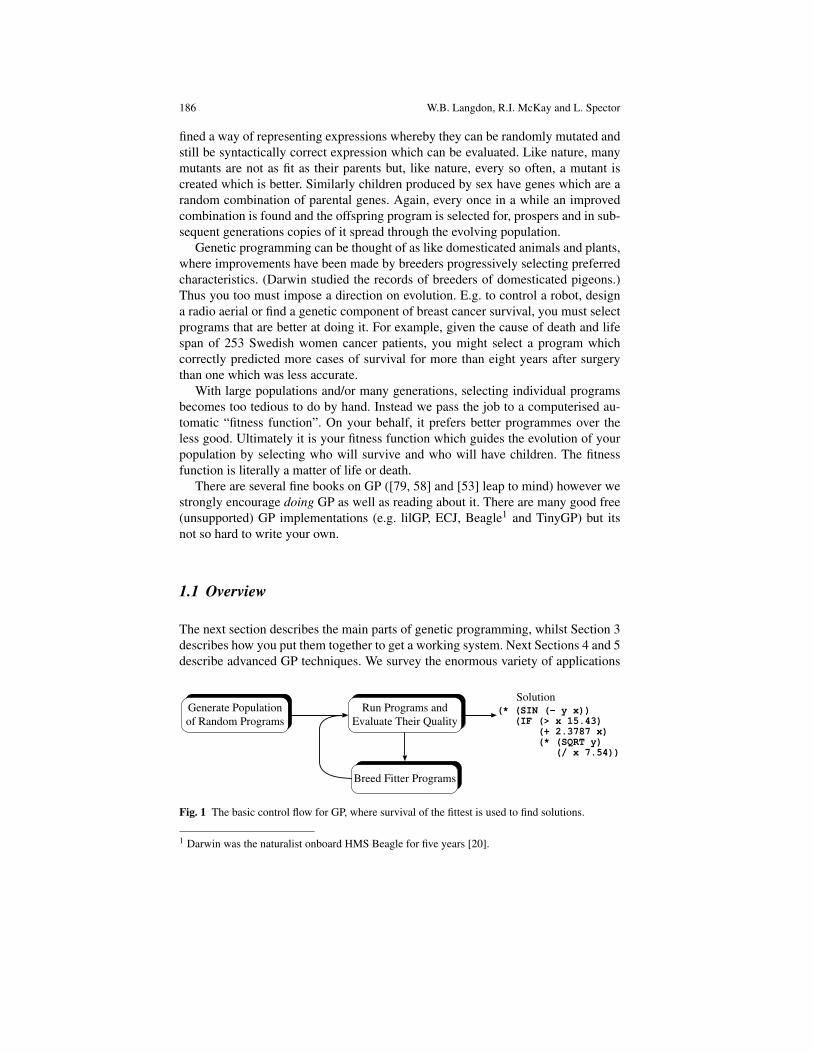
Genetic programming [79] works by applying the power of evolution by naturalselection [21] to artificial populations inside your computer, cf. Figure 1. Unlikein nature, you decide who is fit, who survives and who has children. Like nature,children are not identical to their parents but suffer random mutations and can becreated by fusing together the genetic characteristics of their parents. Unlike otherapproaches to evolving expressions, genetic programming works because it has de-
William B. LangdonComputer Science, Department of Computer Science, University College London, Gower Street,London WC1E 6BT, UKe-mail: [email protected]
Robert I. McKaySchool of Computer Science and Engineering, Seoul National University, Seoul, Koreae-mail: [email protected]
Lee SpectorSchool of Cognitive Science, Hampshire College, Amherst, MA, USAe-mail: [email protected]
Preprint. M. Gendreau, J.-Y. Potvin (eds.), Handbook of Metaheuristics,International Series in Operations Research & Management Science 146, pp 185-225.DOI 10.1007/978-1-4419-1665-5 7 Springer Science+Business Media, LLC 2010
185
186 W.B. Langdon, R.I. McKay and L. Spector
fined a way of representing expressions whereby they can be randomly mutated andstill be syntactically correct expression which can be evaluated. Like nature, manymutants are not as fit as their parents but, like nature, every so often, a mutant iscreated which is better. Similarly children produced by sex have genes which are arandom combination of parental genes. Again, every once in a while an improvedcombination is found and the offspring program is selected for, prospers and in sub-sequent generations copies of it spread through the evolving population.
Genetic programming can be thought of as like domesticated animals and plants,where improvements have been made by breeders progressively selecting preferredcharacteristics. (Darwin studied the records of breeders of domesticated pigeons.)Thus you too must impose a direction on evolution. E.g. to control a robot, designa radio aerial or find a genetic component of breast cancer survival, you must selectprograms that are better at doing it. For example, given the cause of death and lifespan of 253 Swedish women cancer patients, you might select a program whichcorrectly predicted more cases of survival for more than eight years after surgerythan one which was less accurate.
With large populations and/or many generations, selecting individual programsbecomes too tedious to do by hand. Instead we pass the job to a computerised au-tomatic “fitness function”. On your behalf, it prefers better programmes over theless good. Ultimately it is your fitness function which guides the evolution of yourpopulation by selecting who will survive and who will have children. The fitnessfunction is literally a matter of life or death.
There are several fine books on GP ([79, 58] and [53] leap to mind) however westrongly encourage doing GP as well as reading about it. There are many good free(unsupported) GP implementations (e.g. lilGP, ECJ, Beagle1 and TinyGP) but itsnot so hard to write your own.
1.1 Overview
The next section describes the main parts of genetic programming, whilst Section 3describes how you put them together to get a working system. Next Sections 4 and 5describe advanced GP techniques. We survey the enormous variety of applications
Generate Populationof Random Programs
Run Programs andEvaluate Their Quality
Breed Fitter Programs
Solution(* (SIN (- y x)) (IF (> x 15.43) (+ 2.3787 x) (* (SQRT y) (/ x 7.54))))
Fig. 1 The basic control flow for GP, where survival of the fittest is used to find solutions.
1 Darwin was the naturalist onboard HMS Beagle for five years [20].
7. Genetic Programming 187
of GP in Section 6. This is followed by a collection of trouble-shooting suggestions(Section 7) and by our conclusions (Section 8).
2 Representation, Initialisation and Operators in Tree-based GP
2.1 Representation
In artificial intelligence it has become accepted wisdom that how information aboutthe application and its solution is stored (i.e. represented internally within the com-puting system) and manipulated by it, is crucial to succesfull implementation. Hugeeffort is spent by very clever people on designing the correct representation.
Genetic programming has ignored this. In GP, the evolved program contains thesolution and “representation” refers to the language evolution uses to write the pro-gram. The same representation might be used in a program evolved to predict breastcancer survival as one evolved to find insider trading in a stock market.
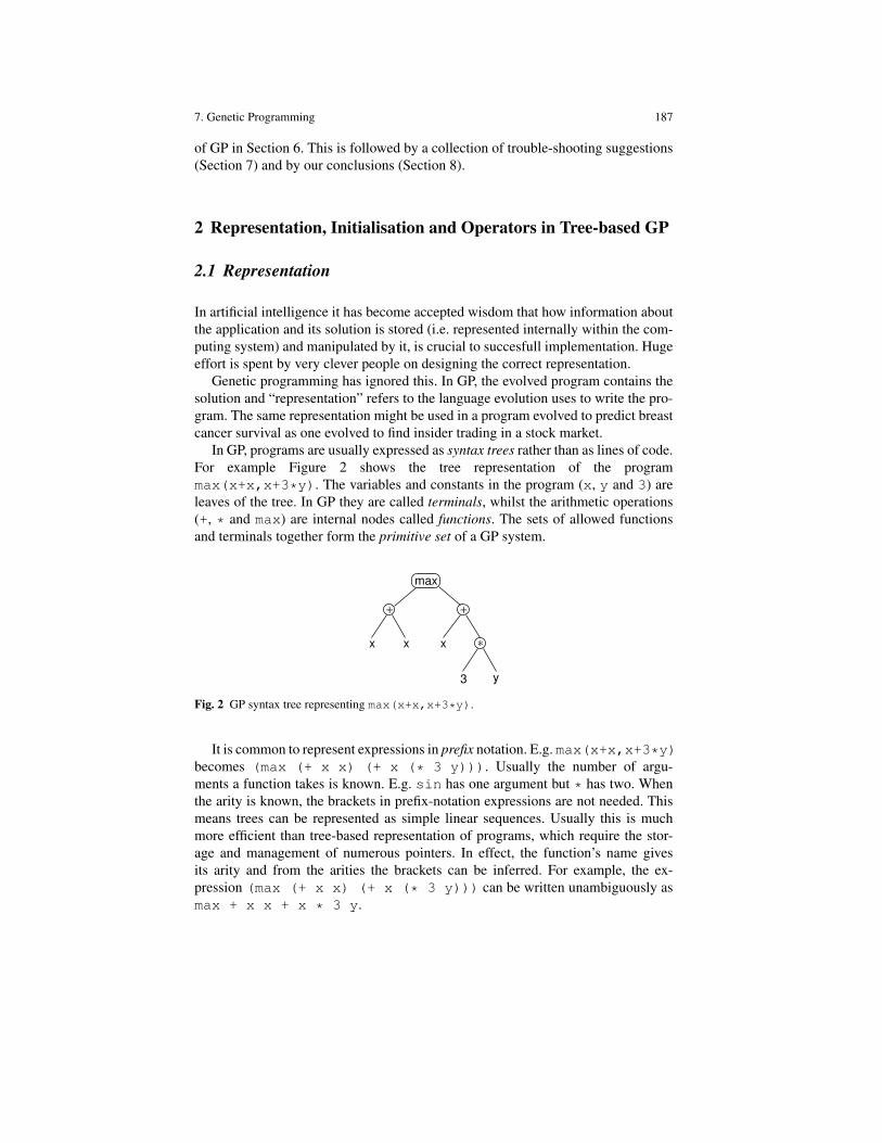
In GP, programs are usually expressed as syntax trees rather than as lines of code.For example Figure 2 shows the tree representation of the programmax(x+x,x+3*y). The variables and constants in the program (x, y and 3) areleaves of the tree. In GP they are called terminals, whilst the arithmetic operations(+, * and max) are internal nodes called functions. The sets of allowed functionsand terminals together form the primitive set of a GP system.
x x
+ +
max
x
y3
∗
Fig. 2 GP syntax tree representing max(x+x,x+3*y).
It is common to represent expressions in prefix notation. E.g. max(x+x,x+3*y)becomes (max (+ x x) (+ x (* 3 y))). Usually the number of argu-ments a function takes is known. E.g. sin has one argument but * has two. Whenthe arity is known, the brackets in prefix-notation expressions are not needed. Thismeans trees can be represented as simple linear sequences. Usually this is muchmore efficient than tree-based representation of programs, which require the stor-age and management of numerous pointers. In effect, the function’s name givesits arity and from the arities the brackets can be inferred. For example, the ex-pression (max (+ x x) (+ x (* 3 y))) can be written unambiguously asmax + x x + x * 3 y.

188 W.B. Langdon, R.I. McKay and L. Spector
The choice of whether to use such a linear representation or an explicit tree repre-sentation is typically guided by convenience, efficiency, the genetic operations beingused (some may be more easily or more efficiently implemented in one represen-tation), and other data one may wish to collect during runs. (It is sometimes usefulto attach additional information to nodes, which may be easier to implement if theyare explicitly represented).
Tree representations are the most common in GP. However, there are other im-portant representations including linear [58, 51, 60, 11] and graph [97, 111, 92]based programs.
2.2 Initialising the Population
As with other evolutionary algorithms, in GP the individuals in the initial populationare typically randomly generated. There are a number of different approaches togenerating this random initial population, e.g. [85]. However we will describe twoof the simplest methods (the full and grow methods), and the most widely usedcombination of the two known as Ramped half-and-half [79].
In both the full and grow methods, the initial individuals are generated so thatthey do not exceed a maximum depth you decide. The depth of a node is the numberof edges that need to be traversed to reach the node starting from the tree’s rootnode (depth 0). The depth of a tree is the depth of its deepest leaf (e.g., the tree inFigure 2 has a depth of 3). The full method generates full trees (i.e. all leaves areat the same depth). It does this by choosing at random from the available functions(known as the function set) until the maximum tree depth is reached. Then the treeis finished by adding randomly chosen leafs from the available terminals (known asthe terminal set). Figure 3 shows a series of snapshots of the construction of a fulltree of depth 2. The children of the * and / nodes must be leaves or otherwise thetree would be too deep. Thus, at steps t = 3, t = 4, t = 6 and t = 7 a terminal mustbe chosen. (In this example leafs x, y, 1 and 0, were randomly chosen).
Although, the full method generates trees where all the leaves are at the samedepth, this does not necessarily mean that all initial trees will have an identicalnumber of nodes (often referred to as the size of a tree) or the same shape. Thishappens only if all the functions have the same arity. (I.e. have the same numberof inputs.) Nonetheless, even when mixed-arity primitive sets are used, the range ofprogram sizes and shapes produced by the full method may be limited. The growmethod creates trees of more varied sizes and shapes. Nodes are selected from thewhole primitive set (i.e., functions and terminals) until the depth limit is reached.Once the depth limit is reached only terminals may be chosen (just as in the fullmethod). Figure 4 illustrates growing a tree with depth limit of 2. In Figure 4 (t=2)the first argument of the + root node happens to be a terminal. This prevents thatbranch from growing any more. The other argument is a function (-). It can growone level before its arguments are forced to be terminals to ensure that the resulting

7. Genetic Programming 189
+t=1
+
∗
t=2 t=3
x
+
∗
+t=4
x
∗
y
+t=6
x
∗
y
/
+t=7
x
∗
y 01
/
+t=5
x
∗
y
/
1
Fig. 3 Creation of a full tree having maximum depth 2 using full initialisation (t = time). [53]
tree does not exceed the depth limit. C++ code for a recursive implementation ofboth the full and grow methods is given in Figure 2.2.
+t=1
+t=2
x
t=3+
−x
t=4+
−x
2
t=5+
−x
2 y
Fig. 4 Creation of a five node tree using the grow initialisation method with a maximum depth of2 (t = time). A terminal is chosen at t = 2, causing the left branch of the root to be closed at thatpoint even though the maximum depth had not been reached [53].
Because neither the grow or full method provide a very wide array of sizesor shapes on their own, Koza proposed a combination called ramped half-and-half[79]. Half the initial population is constructed using full and half is constructedusing grow. This is done using a range of depth limits (hence the term “ramped”)to help ensure that we generate trees having a variety of sizes and shapes.
While these methods are easy to implement and use, the sizes and shapes of thetrees generated are highly sensitive to the number of functions, the number of inputsthey have and the number of terminals. This makes it difficult to control the sizes andshapes of the trees. For example if there are many more terminals than functions, the
190 W.B. Langdon, R.I. McKay and L. Spector
//Choose desired depth uniformly at random between min and max depth.//Choose either full or grow.SubInit(rnd(max_depth-min_depth)+min_depth, rnd(2), min_depth);
void Individual::SubInit(int depth, BOOL isfull, int min_depth) {if (depth <= 0)i=rand_terminal(); // terminal required
else if (isfull || min_depth>0)i=rand_function(); // function required
else {//grow: terminal allowed 50% of the timeif (rnd(2)) // terminal requiredi=rand_terminal();
else // node requiredi=rand_function();
}SETNODE(code[ip],i); //store opcode in Individualip++;
for(int a=0;a<argnum(i);a++) {SubInit(depth-1,isfull, min_depth-1, tree);
}}
C++ code fragment to create a random tree. For efficiency the tree is flattened and stored in arraycode (access is via macro SETNODE). SubInit recursively calls itself until it reaches a leaf ofthe tree. (Based upon Andy Singleton’s GPquick.)
grow method will almost always generate very short trees regardless of the depthlimit. Similarly, if the number of functions is considerably greater than the numberof terminals, then the grow method will be like the full method.
The initial population need not be entirely random. If something is known aboutlikely properties of the desired solution, trees having these properties can be used toseed the initial population.
2.3 Selection
As with other evolutionary algorithms, in GP better individuals are more likely tohave more child programs than inferior individuals. Tournament selection is mostoften used, followed by fitness-proportionate selection [63], but any standard evolu-tionary algorithm selection mechanism (e.g. stochastic universal sampling) can beused.
In tournament selection a number of individuals are chosen at random from thepopulation. These are compared with each other and the best of them is chosen tobe the parent. When doing crossover, two parents are needed and, so, two selectiontournaments are made. Note that tournament selection only looks at which programis better than another. It does not need to know how much better. This effectivelyautomatically rescales fitness, so that the selection pressure is constant. Thus, a sin-

7. Genetic Programming 191
3
1y
∗
+
yx
+
+
2x
/
CrossoverPoint
CrossoverPoint
3
+
2x
/
(x+y)+3
(y+1) (x/2)*
(x/2)+3
Parents Offspring
GARBAGE
Fig. 5 Example of subtree crossover. Note that the trees on the left are actually copies of theparents. So, their genetic material can freely be used without altering the original individuals [53].
gle extraordinarily good program cannot immediately swamp the next generationwith its children. If it did, this would lead to a rapid loss of diversity with poten-tially disastrous consequences for a run. Conversely, tournament selection amplifiessmall differences in fitness to prefer the better program even if it is only marginallysuperior to the other individuals in a tournament.
Tournament selection, due to the random selection of programs to be includedin the tournament, is inherently noisy. So, while preferring the best, tournamentselection does ensure that even below average programs have some chance of havingchildren. Since tournament selection is easy to implement and provides automaticfitness rescaling, it is commonly used in GP.
2.4 Recombination and Mutation
Crossover (recombination) and mutation in GP are very different from crossoverand mutation in other evolutionary algorithms. The most commonly used form ofcrossover is subtree crossover. Given two parents, subtree crossover randomly (andindependently) selects a crossover point (a node) in each parent tree. Then, it createsthe offspring by replacing the subtree rooted at the crossover point in a copy of thefirst parent with a copy of the subtree rooted at the crossover point in the secondparent [79], as illustrated in Figure 5.

192 W.B. Langdon, R.I. McKay and L. Spector
3
yx
+
+
MutationPoint
Randomly GeneratedSub-tree
y
∗
2x
/
yx
+
+
MutationPoint
y
∗
2x
/
Parents Offspring
Fig. 6 Example of subtree mutation [53].
Typical GP primitive sets lead to trees with an average arity of at least two.This means most of the program will be leaves. So if crossover points were chosenuniformly, crossovers would frequently swap very small subtrees (even just leafs).I.e. exchange only very small amounts of genetic material. Whereas in nature (andmany GAs) often both parents contribute more-or-less equally to their offspring’sgenetic code. To counter this, Koza suggested the widely used approach of choos-ing functions 90% of the time and leaves 10% of the time [79]. Many other types ofcrossover and mutation of GP trees are possible (see [53, pp 42–44]).
The most commonly used form of mutation in GP is subtree mutation. It ran-domly selects a mutation point in a tree and substitutes the subtree rooted there witha randomly generated subtree (cf. Figure 6 and [3]).
Another common form of mutation is point mutation, which is GP’s rough equiv-alent of the bit-flip mutation used in genetic algorithms [63]. In point mutation, arandom node is selected and the primitive stored there is replaced with a differentrandom primitive of the same arity taken from the primitive set. If no other primi-tives with that arity exist, nothing happens to that node (but other nodes may still bemutated). When subtree mutation is applied, it changes exactly one subtree. On theother hand, every node in the tree has a small probability of being mutated by pointmutation. This means point mutation independently changes a random number ofnodes.
In GP normally only one genetic operator is used to create each child. Whichone is used is chosen at random. Typically, crossover is applied with the highestprobability, the crossover rate often being 90% or higher. On the contrary, the mu-tation rate is much smaller, typically being in the region of 1%. If the sum of allthe probabilities comes to less than 100% the remaining offspring are created sim-

7. Genetic Programming 193
ply by copying better individuals from the current population. (This is known asreproduction.)
3 Getting Ready to Run Genetic Programming
3.1 Step 1: Terminal Set
GP is not typically used to evolve programs in the familiar languages people nor-mally write programs in. Instead simpler programming languages are used. IndeedGP can usually be thought of as evolving executable expressions rather than fullyfledged programs. The first two preparatory steps, the definition of the terminal andfunction sets, specify the language. Together they define the ingredients that areavailable to GP to create computer programs.
Typically the terminal set contains the program’s inputs. (e.g., x, y, cf. Table 1).It may also contain functions with no arguments. They might be needed becausethey return different values each time they are used, such as a function which returnsrandom numbers, or returns the distance from a robot to an obstacle or because thefunction produces side effects. Functions with side effects may: change some globaldata structures, draw on the screen, print to a file, control the motors of a robot, etc.
Often an evolved program will need access to constants. We dont know in ad-vance what their values will be, so GP choses some randomly. In some implemen-tations the number of constants is limited and it may be that new ones cannot becreated during the GP run. Instead their values must be chosen as the population isinitialised. Typically this done by a special terminal that represents an ephemeralrandom constant. Every time it is chosen (either at the start or when a new subtreeis created by mutation), a different random value is generated. This is used for thatparticular terminal, and remain fixed for the rest of the run.
3.2 Step 2: Function Set
The function set typically contains only the arithmetic functions (+, -, *, /).However, all sorts of other functions and constructs typically encountered in com-puter programs can be used, see Table 1. Sometimes specialised functions or ter-minals, which are designed to solve particular problems are used. For example,if the goal is to evolve art, then the function set might include such actions asselect from pallet and paint.
For GP to work effectively, most function sets are required to have an importantproperty known as closure [79]. Closure can be broken down into type consistencyand evaluation safety. Finally the primitive set must be able to (i.e. must be sufficientto) express solutions to the problem.
194 W.B. Langdon, R.I. McKay and L. Spector
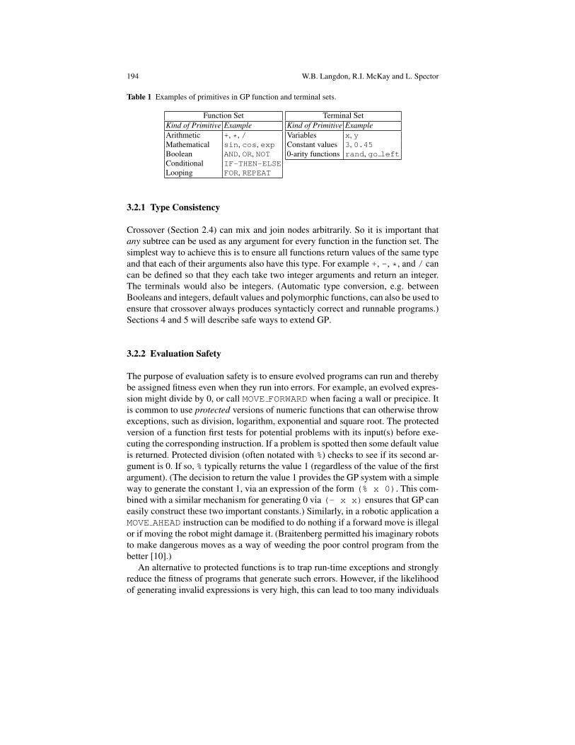
Table 1 Examples of primitives in GP function and terminal sets.
Function SetKind of Primitive ExampleArithmetic +, *, /Mathematical sin, cos, expBoolean AND, OR, NOTConditional IF-THEN-ELSELooping FOR, REPEAT
Terminal SetKind of Primitive ExampleVariables x, yConstant values 3, 0.450-arity functions rand, go left
3.2.1 Type Consistency
Crossover (Section 2.4) can mix and join nodes arbitrarily. So it is important thatany subtree can be used as any argument for every function in the function set. Thesimplest way to achieve this is to ensure all functions return values of the same typeand that each of their arguments also have this type. For example +, -, *, and / cancan be defined so that they each take two integer arguments and return an integer.The terminals would also be integers. (Automatic type conversion, e.g. betweenBooleans and integers, default values and polymorphic functions, can also be used toensure that crossover always produces syntacticly correct and runnable programs.)Sections 4 and 5 will describe safe ways to extend GP.
3.2.2 Evaluation Safety
The purpose of evaluation safety is to ensure evolved programs can run and therebybe assigned fitness even when they run into errors. For example, an evolved expres-sion might divide by 0, or call MOVE FORWARD when facing a wall or precipice. Itis common to use protected versions of numeric functions that can otherwise throwexceptions, such as division, logarithm, exponential and square root. The protectedversion of a function first tests for potential problems with its input(s) before exe-cuting the corresponding instruction. If a problem is spotted then some default valueis returned. Protected division (often notated with %) checks to see if its second ar-gument is 0. If so, % typically returns the value 1 (regardless of the value of the firstargument). (The decision to return the value 1 provides the GP system with a simpleway to generate the constant 1, via an expression of the form (% x 0). This com-bined with a similar mechanism for generating 0 via (- x x) ensures that GP caneasily construct these two important constants.) Similarly, in a robotic application aMOVE AHEAD instruction can be modified to do nothing if a forward move is illegalor if moving the robot might damage it. (Braitenberg permitted his imaginary robotsto make dangerous moves as a way of weeding the poor control program from thebetter [10].)
An alternative to protected functions is to trap run-time exceptions and stronglyreduce the fitness of programs that generate such errors. However, if the likelihoodof generating invalid expressions is very high, this can lead to too many individuals

7. Genetic Programming 195
in the population having nearly the same (very poor) fitness. This makes it hard forselection to choose which individuals might make good parents.
3.2.3 Sufficiency
By sufficiency we mean it is possible to express a solution to the problem using theelements of the primitive set. For example {AND, OR, NOT, x1, x2, ..., xN}. is a suf-ficient primitive set for logic problems, since it can produce all Boolean functionsof the variables x1, x2, ..., xN. The primitive set {+, -, *, /, x, 0, 1, 2}, is unableto represent transcendental functions, such as sin(x). When a primitive set is insuffi-cient, GP can often develop programs that approximate the desired solution. Whichmay be good enough for the user’s purpose. Adding a few unnecessary primitives inan attempt to ensure sufficiency tends not to slow down GP overmuch.
3.3 Step 3: Fitness Function
The task of the fitness measure, is to choose which parents are to have offspring.That is, which parts of the search space we have just sampled, (which is what thecurrent population has done for us) are worth exploring further. The fitness func-tion is our primary (and often sole) mechanism for giving a high-level statement ofrequirements to GP.
Fitness can be measured in many ways. For example, in terms of: the amount oferror between its output and the desired output; the amount of time (fuel, money,etc.) required; the accuracy of the program in recognising patterns or classifyingobjects; the payoff a game-playing program produces.
Fitness evaluation normally requires executing all the programs in the population,typically multiple times. While one can compile the GP programs that make up thepopulation, the overhead of building a compiler is usually substantial, so it is muchmore common to use an interpreter to evaluate the evolved programs. Interpreting aprogram tree means executing the nodes in the tree in an order that guarantees thatnodes are not executed before the value of their arguments (if any) is known. Thisis usually done by traversing the tree recursively starting from the root node, andpostponing the evaluation of each node until the values of its children (arguments)are known. Other orders, such as going from the leaves to the root, are possible.If none of the primitives have side effects, the two orders are equivalent. Figure 7contains C++ code fragments which implements top down recursive tree evaluationusing a linear data structure for speed.
In some problems we are interested in the output produced by a program. In otherproblems we are interested in the actions performed by a program composed offunctions with side effects. In either case the fitness of a program typically dependson the results produced by its execution on many different inputs or under a varietyof different conditions. For example the program might be tested on all possible

196 W.B. Langdon, R.I. McKay and L. Spector
//Flatted tree is stored in array of nodes.//evalnode has three components. It trades space for speed.//node (not shown) stores the same information in one byte. It//is used to store the population. node is expanded to evalnode//before fitness testing.//typedef allows code to be compiled for several applications.
typedef float retval;typedef retval (*EVALFUNC)(); // evaluation code with global pointertypedef struct evalnode {EVALFUNC ef;evalnode* jump;retval value;
} evalnode; // node type
evalnode* IP; //global pointerevalnode* ExprGlobal; //Array holding flatten tree//some old Sun compilers incorrectly optimise EVAL (workaround via FTP)#define EVAL ((++IP)->ef)()#define GETVAL IP->value#define TRAVERSE() IP=(++IP)->jump
retval D0Eval() { return data[0]; } //data holds inputs D0-D9. Typically itretval D9Eval() { return data[9]; } //is different for each training caseretval ConstEval() {return GETVAL;}retval AddEval() {return EVAL + EVAL;}retval SubEval() {return EVAL - EVAL;}retval MulEval() {return EVAL * EVAL;}retval DivEval() {// "Protected" divisionconst retval numerator = EVAL;const retval denominator = EVAL;if (denominator !=0) return numerator/denominator;else return 1;
}retval IflteEval() {//IfLTE(condition1islessthan,condition2,dothis,dothat)retval rval=EVAL;if (rval<=EVAL) {rval=EVAL;TRAVERSE(); // Jump the third expression
} else {TRAVERSE(); // Jump the second expressionrval=EVAL;
}return rval;
}
retval Individual::evalAll() {// eval the whole expression anewIP=ExprGlobal-1; // start at begining of flatten treereturn EVAL;
}
Fig. 7 Example fast interpreter (based on Andy Singleton’s GPquick). The tree is linearised andfunctions and terminals within it are replaced by pointers to C++ functions which implementsthem. On a typical modern computer the GP individual and the interpreter are held in fast cache.Since the tree is flatten into the traditional depth first order, the interpreter runs from top of thetree to the rightmost terminal in one forward pass. This avoids backtracking. Continuous forwardmotion suits typical cache architectures.
7. Genetic Programming 197
combinations of inputs x1, x2, ..., xN. Alternatively, a robot control program mightbe tested with the robot in a number of starting locations. These different test casestypically contribute to the fitness value of a program incrementally, and for thisreason are called fitness cases.
Despite all this sophistication and the computational work it does, the fitnessfunction ultimately boils down to just one bit of information: does this mutatedprogram beget another child? We don’t know the correct answer to this question.So we add noise (e.g. via tournament selection). Fortunately it is not necessary toget the answer right all the time, or even most of the time, just as long as we areright occasionally. We sometimes lose sight of this hard truth. Sometimes it maybe better to accept a less accurate calculation of fitness. If by doing so we reducethe time taken to calculate a fitness value. Thus allowing us to take the life or deathdecision more times.
3.4 Step 4: GP Parameters
The most important control parameter is the population size. It is impossible tomake general recommendations for setting optimal parameter values, as these de-pend too much on the details of the application. However, genetic programming isin practice robust, and it is likely that many different parameter values will work.As a consequence, one need not typically spend a long time tuning GP for it to workadequately. Some possible parameter settings are given in the tableau in Table 2.
3.5 Step 5: When to Stop and How to Decide Who is the Solution
The last step, is choosing when to stop the GP and how to decide which of thethousands of programs that it has evolved to use. Typically we stop either when anacceptable solution has been found or a maximum number of generations has beenreached. Typically, the single best-so-far individual is used. Although one mightwish to study additional individuals. E.g. to look for particularly short or elegantsolutions.
4 Guiding GP with a priori Knowledge
As described so far, GP is essentially knowledge-free: a powerful search mechanism(evolution) is set free to search the space of all expressions which can be formedfrom the function and terminal set. Contrast this with traditional methods, such aslinear regression, in which a very basic search mechanism is used to search a veryrestricted set of expressions. Linear regression is often extended to more complex

198 W.B. Langdon, R.I. McKay and L. Spector
Table 2 Typical parameters for example genetic programming run
Objective: Record your problem hereFunction set: For example: +, −, % (protected division), and ×; all operating on floatsTerminal set: For example: x, and constants chosen randomly between −5 and +5Fitness: E.g. sum of absolute errors for a number of fitness cases.
The number of fitness cases may be limited by the amount of training data availableto evaluate the fitness of the evolved individuals. In other cases, e.g. 22-bit evenparity [52], there can be too much training data. Then the fitness function may use afraction of the training data. This does not necessarily have to be done manually asthere are a number of algorithms that dynamically change the test set as the GP runs(see [53, Sect. 10.1]).
Selection: Tournament size 7Initial pop: Ramped half-and-half (Section 2.2) depth range of 2–6Parameters: As a rule one prefers to have the largest population size that your system can handle
gracefully. Normally the population size should be at least 500, and people often usemuch larger populations. (However some prefer much smaller populations. Typicallythese rely on mutation rather than crossover. and run many more generations.)Traditionally, 90% of children are created by subtree crossover. However, the use ofa 50-50 mixture of crossover and a variety of mutations also appears to work well[53, Chapter 5].Some implementations do not require arbitrary limits of tree size. Even so, becauseof bloat (the uncontrolled growth of program sizes during GP runs [53, Sect. 11.3]),it is common to impose either a size or a depth limit or both (see Section 7.6).
Termination: 10–50 (The most productive search is usually performed in those early generations.)
forms (polynomial regression, log regression etc.), but this still leaves a vast gapbetween the complete search of GP, and the very restricted parameter search ofclassical regression.
In many applications, the user will know a great deal about the form of acceptablesolutions. It can be highly desirable to incorporate this knowledge into the search,since it can save the user time, e.g. by enabling the user to exclude solutions whichwill not be useful for some reason, or to impose a preference ordering on solutions.Including the user’s background knowlege can also increase data efficiency, and soallow more complex models to be learnt than could possibly be justified solely bythe available data. In some cases, such restriction may be essential, because it maynot be possible to provide meaningful fitness values for all the solutions a GP systemcould evolve. Finally, GP search may be more efficient if the user’s knowledge canbe used to increase the concentration of solutions in the search space. This increasemay be non-trivial (in Example 3 below it is many orders of magnitude) but it isnevertheless the least important reason.
In principle, a wide range of mechanisms could be used to restrict the searchspace; in practice, most available systems use some form of grammar, generally anextension of Context Free Grammars (CFG [16]). The constraints may range over awide range of complexity, for example:
1. Strongly-typed systems (Section 3.2.1, [93]), in which only type-consistent ex-pressions can be evolved.
7. Genetic Programming 199
2. Extended process models: in many domains, such as ecological modelling [32],there is a known sub-model of processes which are certainly occurring (zoo-plankton are eating phytoplankton, for example), but there may also be otherunknown processes occurring which require adaptation of this process model tofit the data.
3. Dimensional consistency [98]. For example, in physics, equations must be con-sistent in time (t), length (l) and mass (m) dimensions. For example integratingNewton’s second equation of motion gives s = ut + 1
2 at2. s has dimensions oflength. u is a velocity and hence has dimension l/t. 1
2 is a pure number and sohas no dimensions. a is an acceleration and hence has dimension l/t2. Puttingthese together, the right hand side gives l/t × t + lt−2 × t2 = l. Which is indeedthe same as the dimensions of the left hand side (l). Dimensionally inconsistentformulae may fit the data well but they are nevertheless unacceptable.
4.1 Context Free Grammars in GP
CFG-based GP systems are the most widely used, and the simplest to explain, sowe take them as our base case. From the user’s perspective, a CFG-GP system isvery similar to a standard GP system. However instead of just providing a list offunction and terminal symbols2, the user must provide a grammar specifying theways in which they may be used. That is the only change really required; the userdoes not have to do anything special with respect to the GP operators (selection,crossover, mutation); the system takes care of those. For some systems, there maybe one further difference. In a grammar-based system, the fitness function can bedefined in the same way as for standard GP. However the grammar defines how tobuild up more complex expressions from simpler ones. In many cases, it is easier todefine how to build up the meanings of the expressions (i.e. how to evaluate them) atthe same time – we call this ’providing a semantics for the grammar’. If this is done,the fitness function definition may reduce to just a few lines of code, defining howthese values contribute to the fitness. We give a brief example in sub-section 4.1.1below.
The grammar provides an additional way for the user to interact with the evolvingpopulation. When the CFG-GP system is first run, it may not produce the resultsthe user desires. E.g. the evolved solution may not fit the data sufficiently well. Orit may not be acceptable to the user for some other reason. However, the CFG-GPruns may help the user see how the problem may be solved. Frequently, it is possibleto incorporate this insight into the grammar so as to achieve more useful results in
2 A word of caution: GP and grammar terminology were both developed before grammar-basedGP systems and use some of the same words. Unfortunately, when they came together in grammar-based GP, some inconsistencies arose. Thus, in a CFG-GP system, a (GP) function symbol is aterminal (in grammar terms), though it is not a member of the GP terminal set. Unfortunately theredoes not seem to be any reasonable way to resolve this inconsistency.

200 W.B. Langdon, R.I. McKay and L. Spector
subsequent runs. This ability to interact with the solution space, through grammardefinitions, is one of the primary practical benefits of grammar-based GP systems.
Of course, the implementation of CFG-GP is a little more complex than sim-ple tree GP, though this is generally not visible to the user. In GP, the individualsof the evolutionary population are expression trees; in CFG-GP, the individuals areparse trees from the grammar. I.e. CFG-GP individuals are paths through the user-supplied grammar, starting from the grammar’s start symbol (the root of the parsetree). Eventually the path will reach terminals of the grammar (i.e. symbols whichcannot be expanded further). The list of terminals (in the order they were encoun-tered) is the output of the grammar. Typically, this list is an executable program(written in the language specified by the user’s grammar). It is then run in order tofind the fitness of the CFG-GP individual.
Initialization, which requires ensuring grammar consistency while guaranteeingto stay within the depth bound, is also a little complex; most systems use a variant ofthe grow-tree algorithm described in Section 2.2. This is combined with a countingmechanism, to ensure that it is always possible to complete a parse tree within theremaining depth. Crossover and mutation are defined in ways that preserve grammarconsistency. Mutation replaces a subtree from the grammar with a random subtree.It creates the random subtree in the same way as the initial population is created, ex-cept that it starts from the location in the grammar occupied by the subtree it has justremoved, rather than at the root. Crossover is essentially like normal GP crossover,except that crossover is only allowed between nodes with the same grammar non-terminal. This ensures, as with mutation, that the offspring is consistent with thegrammar.
4.1.1 Example of CFG-GP: Strong Typing in GP
We use Strongly Typed GP [93] as a simple example of grammar use. A GP prob-lem requiring two types, arithmetic and Boolean, might use a grammar such as inTable 3. Thus the first “arithmetic” rule says that an arithmetic expression may con-sist of the sum of two arithmetic expressions, or (| means or) the difference of twoarithmetic expressions, and so on. The second “interaction” rule says that a Booleanexpression may be formed by comparing two arithmetic expressions, with any of thecomparison operators <, = or >. Thus the grammar permits arbitrarily complex nest-ing of arithmetic and Boolean expressions, but guarantees that they are combined inmeaningful ways.
In systems which also support semantic specification within the rules, a rule suchas A → A∗A would be expanded to include variables. These variables represent thevalues generated by the rule (such as A(A0) → A(A1) ∗ A(A2)). Extra (semantic)rules then give the values of those variables (such as val(A0) = val(A1) * val(A2)).Of course, in simple cases like this, where the meaning of ’*’ is already built intothe language in which the GP system is written, the advantage is limited. In morecomplex domains, or problems where other properties of the expression in addition

7. Genetic Programming 201
Table 3 An example grammar for Boolean and arithmetic types. The following six rules definehow non-terminal symbols A (the start symbol, representing arithmetic expressions) and B (repre-senting Boolean expressions) can be expanded into 15 (grammar) terminals +−∗/ x 0 if(, , ) < => & ∨ ¬ true false.
Arithmetic RulesA → A+A|A−A|A∗A|A/AA → x | 0
Interaction RulesA → if(B, A, A )B → A < A|A = A|A > A
Boolean RulesB → B&B|B∨B ¬BB → true | false
to its value may be needed, semantic specification can greatly simplify coding theproblem.
4.2 Variants of Grammar-Based GP
4.2.1 More Powerful Grammars
Perhaps the most important issue is that the user’s knowledge may not be express-ible in context-free form. This has led to a wide range of extended-grammar sys-tems. They fall into two main classes: Context Sensitive Grammars (CSG) [116]and attribute and other semantic grammars [68].
CSG permit more precise syntactic restrictions on the search space; for someproblem domains, this greater expressiveness is important for encoding the problem.
Attribute grammars extend the semantic specification we described in Sec-tion 4.1.1. In some problems, the semantics may allow us to decide early in theevaluation process, that the individual will have low fitness. For example, in a con-straint problem, we may know that if a constraint is breached early in evaluating anindividual, the violation is only going to get worse as we continue with its evalua-tion. Thus semantic constraints may be used to short-circuit fitness evaluation. Buteven more intriguingly, they may be used to avoid creating poor individuals at all.For example, when we come to cross over individuals, the semantic values attachedto the nodes in an individual might indicate that a crossover at a particular pointwould automatically breach a constraint. A system based on semantic grammarscan then simply abort the crossover, never creating the potentially poor individual.In general, if it is difficult to express the user’s knowledge about the search space ina CFG, consider using either a CSG or a semantic grammar.
4.2.2 More Flexible Representations: GE and Tree Adjunct Grammars
The reduction in search space size provided by a CFG representation can be ben-eficial for search; but it comes at a cost. The CFG reduces not only the numberof formulae that can be represented in the search space, but also the links betweenthem. Paradoxically, in some cases this sparser search space might be more difficult

202 W.B. Langdon, R.I. McKay and L. Spector
for evolution to search than the original search space. Two approaches have beenintroduced to avoid this problem. In the first [95, 28], the CFG representation islinearized: instead of representing the individuals directly as grammar parse trees,a coding scheme represents them as linear strings. This approach has led to one ofthe most widely used GP systems, known as Grammatical Evolution (GE) [28]. Theother [48] uses an alternative representation from natural language study, Tree Ad-junct Grammars (TAGs [70]); unlike CFG trees, any rooted subtree of a TAG tree issyntactically and semantically meaningful, so that there is much more flexibility intransforming one TAG tree to another.
In both cases, the syntactic flexibility provides an additional benefit: it is rel-atively easy to implement new operators (often analogous to biological processesthat occur in DNA evolution) which may simplify search in particular domains.Practically, this means that where search with standard-GP and CFG-GP systemshas stagnated, it may be worth investigating GE or TAGs. They may be able to solveproblems which are beyond the reach of more classical GP systems.
4.2.3 Grammar Learning
A number of more experimental grammar-based systems [99, 59, 9] refine the gram-mar describing the search space as search proceeds. (These systems are usuallybased on probabilistic grammars: each grammar rule option has a probability at-tached to it, indicating the probability that it will be used in generating an individ-ual.) This has two consequences. It can make for faster search. But more impor-tantly, it means that the grammar at the end of the search space may give an explicitrepresentation of the space of solutions (rather than the implicit representation givenby the best individuals in a final GP population).
This explicit representation may be of value in its own right, especially in appli-cations such as scientific research, where the desired outcome is better understand-ing of the processes in the domain, rather than simply predictive models. The use ofprobabilistic grammars means that the understanding may be quite sensitive, goingbeyond just the content of the grammar rules. In some parts of the grammar, theprobabilities may converge close to either 1.0 or 0.0, indicating that that aspect ofthe grammar is important in defining a solution to the problem; in others, the prob-abilities may be more widely spread, indicating that that aspect of the grammar isnot particularly important to the problem solution.
5 Expanding the Search Space in Genetic Programming
In Section 4 we described some of the ways in which you can give the evolutionaryprocess a helping hand. For example, by providing domain-specific data types or byconstraining programs to conform to an appropriate grammar. But, in the context ofa particular problem or a particular set of program representations, we don’t nec-

7. Genetic Programming 203
essarily know how to give evolution a helping hand. In which case it can be usefulto expose more, rather than less, of the system’s decisions about data and controlarchitecture to evolution. Doing so will often incur new costs, some from the addedcomplexity of the system and some from the expansion of the space of programswhich GP is searching [86]. However in many cases these costs can be justified byimprovements to problem solving power or scalability.
We will discuss some of the ways in which researchers have expanded thepurview of the evolutionary process in GP. In Section 5.1, we first examine theevolution of data structures and the ways in which they can be accessed and ma-nipulated by evolving programs. We then turn to program and control structure.Section 5.2 describes how GP can be used to evolve programs that use subroutines,macros, and more exotic techniques for controlling the flow of execution. The con-cept of “development” (here development means the evolved programs build otherstructures which then produce the desired behaviors) provides for even more evolu-tionary flexibility (Section 5.3). The last part of this section (5.4) describes mecha-nisms by means of which the evolutionary processes themselves can be allowed toevolve.
5.1 Evolving Data Structures and their Use
The earliest and simplest GP applications evolved programs that used single, simpledata types. The use of multiple—but still simple—data types has been helped in avariety of ways, for example by the use of strong typing (see Section 4 and [93]).An important technique for evolving programs that use more complex data types isindexed memory, which was first presented by Teller [110]. An indexed memory issimply an array of variables of some simple type, accessed using integer indices.Teller showed that by including indexed memory read and write functions inthe GP function one can evolve programs that use memory in relatively complexand useful ways. He also showed that the inclusion of indexed memory was usefulin expanding the space of programs over which GP can search. E.g. it can be shownto include programs for all Turing computable functions.
Indexed memory can be used by evolving programs to implement a wide varietyof more complex data structures, but modern software engineering practice suggeststhat it is even more useful for human programmers—and hence possibly also forGP—to have access to higher-level data structures. Langdon has investigated theextent to which GP can evolve, and subsequently use, more abstract data structuresincluding stacks, queues and lists [84]. He showed that GP can indeed evolve andsubsequently solve problems using such data structures, and that GP with abstractdata types can outperform GP with indexed memory on several problems, includinga context free language recognition problem and the problem of implementing asimple four function calculator.
Alternative program representations provide additional opportunities for the evo-lution and use of data structures. For example, approaches based on polymorphic

204 W.B. Langdon, R.I. McKay and L. Spector
functional representations, initially developed by Yu using Haskell [121], have re-cently been extended by Binard and Felty, using a version of the λ -calculus to whichthey have added an operation of abstraction on types [8]. They showed how their sys-tem could evolve and use abstractions for Boolean and list data types which werenot explicitly present in their initial environments.
To some extent, the ways in which data types and program syntax are interre-lated determine the ways in which GP can discover and use complex data struc-tures. Strongly typed GP and polymorphic GP provide two approaches but they donot exhaust the possibilities. For example, in the Push programming language allcommunication between instructions is accomplished via typed global data stacks.It is not specified by placing the instructions next to each other, as in most pro-gramming languages. This decouples an evolving program’s type structures fromits control structures and thereby permits greater flexibility (for good or ill) in theexpression of programs that manipulate multiple data types [107, 45].
5.2 Evolving Program and Control Structure
Most interesting programs that are written by humans involve the use of controlstructures not available in the simplest GP systems. These include mechanisms thatsupport iteration, recursion, and the definition and use of reusable code modules.As with data structures, GP researchers have developed a range of techniques forevolving programs that evolve and use these powerful control abstractions.
Limited forms of iteration are relatively easy to handle through the use of primi-tive functions that simply repeat the execution of a subexpression some specifiednumber of times. This was demonstrated in Koza’s first book using do untilstructures [79]. A variety of more sophisticated techniques, such as the “restrictediteration creation” operations of Koza and Andre [81], have been developed to helpGP systems incorporate iteration into evolving programs. Both iteration and recur-sion present challenges with respect to nontermination; this is generally handledeither by imposing execution limits or by using primitives that are naturally self-limiting, such as the foldr function in Haskell [118]. While the search space ofrecursive programs appears to be rugged, and several early attempts to evolve recur-sive programs produced negative results (e.g. [115]), more recent research has beenincreasingly successful (e.g. [12, 118, 117, 119, 45, 1]).
Modular structures can also be incorporated into evolving programs in severalways. A common approach, pioneered by Koza [80], is to simultaneously evolve a“main program” (sometimes called a “result producing branch”) and one or more“automatically defined function” (ADF) branches that can be called by the mainprogram and possibly by each other (usually with restrictions to prevent nontermi-nating recursion). This approach has been shown to provide dramatic advantages incertain problem areas with exploitable regularities. In the original ADF frameworkthe number of ADFs and the numbers of arguments that they take are specified man-

7. Genetic Programming 205
ually, but the subsequent development of “architecture altering operations” broughtthese decisions, as well, under evolutionary control [38].
A variety of other approaches to the evolution and use of modules have also beendeveloped. For example, in “evolutionary module acquisition” the code for modulesis not evolved in separate branches but rather is extracted from the main programsof relatively successful individuals in the population [4, 74, 114]. “Automaticallydefined macros” allow GP to evolve not only function modules but also controlstructure modules that execute code conditionally or repeatedly [102]. And severalresearchers have shown how GP can be used to evolve object-oriented programs inwhich functionality is modularized through the use of classes and objects [14, 87].
More radical forms of control structure evolution have also been explored. Forexample, the inclusion of combinators (higher-order functions studied in the theoryof functional programming languages) in the function set can allow GP to explorea large space of control architectures while imposing minimal constraints on pro-gram syntax [45, 13]. Perhaps the greatest flexibility—and therefore potentially themost intractable search space— is provided by the Push programming language, inwhich programs can contain arbitrary code-manipulation instructions and therebytransform their own code in arbitrary ways during execution [107, 45]. All of theseinnovations have been demonstrated to be useful in certain circumstances, but fur-ther study is required to determine exactly when.
5.3 Evolving Development
In nature an organism’s genes do not interact directly with its environment; rather,they direct the construction of proteins which form the organism’s body. It is thatbody—the phenotype—that interacts with the organism’s environment.
Several GP techniques have been inspired by the biological distinction betweengenotype and phenotype, and by the process, called ontogeny, by which the geno-type leads to the phenotype (e.g. [6, 69, 108, 54]). In the most common approach,developmental GP, the programs produced by GP are structure-building programs,and it is the structures that are built by these programs, rather than the programsthemselves, that are tested for fitness in the problem environment.
Typically one begins the developmental process with an “embryo” that consistsof a minimal structure of the appropriate kind. The functions in the GP function setthen, when executed, augment this embryo. For example, if the desired structure isa neural network then the embryo might consist of a single input node connected toa single output node and the functions in the GP function set might add additionalnodes and connections [65]. Or if the desired structure is an electrical circuit thenthe embryo might consist of a voltage source connected to a load resistance and thefunctions in the GP function set might add components and wires [38].
The developmental approach has been successful in a wide range of applica-tion areas, ranging from the evolution of control systems [40] to the evolution ofquantum circuits [103]. Part of its appeal comes from the way that it facilitates the

206 W.B. Langdon, R.I. McKay and L. Spector
application of GP to the evolution of structures that are not themselves best viewedas computer programs; developmental GP still evolves computer programs, but theprograms build (develop) structures that might be quite different in nature fromcomputer programs. Other attractions of developmental GP may derive from waysin which it affects the GP search process. For example, one might expect mutationto have a different range of effects when applied early in a developmental processthan when applied to the fully developed phenotype (as is done in standard GP).Whether this will be the case, and whether a developmental approach will thereforehelp or hinder, will depend on the specific problem and program representations.In biology, however, evolution often proceeds through adjustments to developmen-tal programs and timing [64], and there is recent evidence that it can also lead todesirable properties such as robustness and self-repair in GP [91].
When the phenotype is not a computer program, developmental GP makes iteasier to apply GP by making it easier to choose the function set. Because of thefreedom that one has in designing a structure-building function set, developmentalGP also allows you to experiment with different genotype-to-phenotype mappings,some of which may be more successful than others.
5.4 Evolving Evolutionary Mechanisms
The most radical expansions of the GP search space involve evolutionary control ofthe evolutionary process itself. There is a long history of research on self-adaptivemechanisms in evolutionary computation (e.g. see [2, 90]). In most areas outsideof GP this means that numerical parameters of the evolutionary algorithm—for ex-ample mutation rates—are themselves encoded in the evolving genomes and arethereby subject to variation and selection. Similar strategies can also be applied toGP, but because GP involves the evolution of programs it is natural to ask whether aGP process can also usefully evolve its own utility programs—for example its utilityprogram for performing mutation—and other aspects of the overall evolutionary al-gorithm along with the main problem-solving programs that are its primary targets.
Several approaches to self-adaptation in GP have been explored. These includeseveral “meta-GP” approaches, in which programs implementing genetic operators(like mutation and crossover) co-evolve with problem-solving programs in separatepopulations [101, 111, 23]. In “autoconstructive evolution” these evolving auxil-iary functions are encoded in the problem-solving programs themselves; much asin biology. Code for reproduction (mate selection, mutation, recombination, etc.)can be intermingled with, and can interact with, code for survival (problem-solvingperformance) in an individual’s genome [107].
The attractions of these techniques, which allow a GP system to evolve itself asit runs, stem from the possibility that the resulting systems will be adapted to theirproblem environments and therefore more effective than hand-designed systems. Aswith the other expansions to the GP search space discussed above, however, there
7. Genetic Programming 207
are significant associated costs and many open research questions about how andwhen these costs can be overcome or justified.
6 Applications
There are more than 5000 recorded uses of GP. These include an enormous numberof applications. It is impossible to list them all. However we shall start with a discus-sion of the general kinds of problems where GP has proved successful (Section 6.1)and the important area of symbolic regression (Section 6.2). Next come sectionswhich review the main application areas of GP: Image and Signal processing (6.3)Finance (6.4) Industrial Process Control (6.5) Medicine and Bioinformatics (6.6)Hyper-heuristics (6.7) Entertainment and Computer Games (6.8) and Art (6.9). Weconclude with a description of some of the human-competitive results automaticallygenerated by GP (Section 6.10).
6.1 Where GP has Done Well
If one or more of the following apply, GP may be suitable.
• The interrelationships among the relevant variables are unknown or poorly un-derstood. GP can help discover which variables and operations are important;provide novel solutions to individual problems; unveil unexpected relationshipsamong variables; and, sometimes GP can discover new concepts. These mightthen be taken and applied as in a conventional way.
• Finding the size and shape of the ultimate solution is a major part of the problem.• Many training data are available in computer-readable form.• There are good simulators to test the performance of tentative solutions to a prob-
lem, but poor methods to directly obtain good solutions.In many areas there are tools to evaluate a completed design. (E.g. how far willthis bridge bend under the forecast load.) Such tools solve the direct problem ofworking out the behaviour of a solution. However, the knowledge held withinthem cannot be easily used to solve the inverse problem of designing an artifactfrom its requirements. GP can exploit simulators and analysis tools and “data-mine” them to solve the inverse problem automatically.
• Conventional mathematical analysis cannot give analytic solutions.• An approximate solution is acceptable.• Small improvements are highly prized. Even in mature applications GP can
sometimes discover small delta improvements, which may be very valuable.
Two examples are NASA’s work on satellite radio aerial design [35] and Spec-tor’s evolution of new quantum computing algorithms that out-performed all pre-vious approaches [43, 44]. Both of these domains are complex, do not have ana-
208 W.B. Langdon, R.I. McKay and L. Spector
lytic solutions, but good simulators existed which were used to define the fitness ofevolved solutions. In other words, people didn’t know how to solve the problemsbut they could (automatically) recognise a good solution when they saw one. Inboth cases GP discovered highly successful and unexpected designs. Also the keycomponent of the evolved quantum algorithm was extracted and applied elsewhere[105].
6.2 Curve Fitting, Data Modelling and Symbolic Regression
There are many very good tools which will fit curves to data, however typicallythey require you to specify the type of curve you want fitted. E.g. a straight line, anexponential, a Gaussian distribution. Where GP can help is where the form of thecurve or underlying model is unknown. In fact the main problem can be discoveringthe form of the solution or which data to use. This is generally known as symbolicregression.
By regression we mean finding the coefficients (e.g. slope and y-intercept) ofa predefined function such that the function best fits some data. However until agood fit is found the experimenter has to keep trying different functions by handuntil a good model for the data is found. Sometimes, even expert users have strongbiases when choosing functions to fit. For example, in many applications there is atradition of using linear models, even when the data might be better fit by a morecomplex model. Since GP does not make this assumption, it is well suited to thissort of discovery task.
For instance, GP can evolve soft sensors [30]. The idea is to evolve a functionwhich estimates what a real sensor would measure, based on data from other actualsensors in the system. (E.g. where placing an actual sensor would be expensive.)Experimental data (e.g. from industrial plant) typically come in large tables wherenumerous quantities are reported. Usually we know which variable we want to pre-dict (e.g., the soft sensor value), and which other quantities we can use to makethe prediction (e.g., the real sensor values). If this is not known, then experimentersmust decide which are going to be their dependent variables before applying GP.Sometimes there are hundreds or even thousands of variables. (In Bioinformatics thenumber of variables may approach a million.) It is well known that in these cases theefficiency and effectiveness of any machine learning or program induction method,including GP, can dramatically drop as most of the variables are typically redundantor irrelevant. This forces the system to waste considerable energy on isolating thekey features. To avoid this, it is necessary to perform some form of feature selection,i.e., we need to decide which independent variables to keep and which to leave out.There are many techniques to do this, its even possible that GP itself can be used todo feature selection [83].
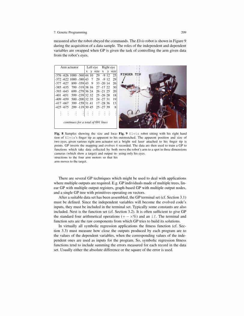
There are problems where more than one output (prediction) is required. Forexample, Table 8 contains data collected from a robot. The left hand side givesfour control variables, whilst the right hand side contains six dependent variables
7. Genetic Programming 209
measured after the robot obeyed the commands. The Elvis robot is shown in Figure 9during the acquisition of a data sample. The roles of the independent and dependentvariables are swapped when GP is given the task of controlling the arm given datafrom the robot’s eyes.
Arm actuator Left eye Right eyex y size x y size
-376 -626 1000 -360 44 10 29 -9 12 25-372 -622 1000 -380 43 7 29 -9 12 29-377 -627 899 -359 43 9 33 -20 14 26-385 -635 799 -319 38 16 27 -17 22 30-393 -643 699 -279 36 24 26 -21 25 20-401 -651 599 -239 32 32 25 -26 28 18-409 -659 500 -200 32 35 24 -27 31 19-417 -667 399 -159 31 41 17 -28 36 13-425 -675 299 -119 30 45 25 -27 39 8
......
......
......
......
......
continues for a total of 691 lines
Fig. 8 Samples showing the size and loca-tion of Elvis’s finger tip as apparent to histwo eyes, given various right arm actuator setpoints. GP inverts the mapping and evolves 4functions which take data collected by bothcameras (which show a target) and output in-structions to the four arm motors so that hisarm moves to the target.
Fig. 9 Elvis robot sitting with his right handoutstretched. The apparent position and size ofa bright red laser attached to his finger tip isrecorded. The data are then used to train a GP tomove the robot’s arm to a spot in three dimensionsusing only his eyes.
There are several GP techniques which might be used to deal with applicationswhere multiple outputs are required. E.g. GP individuals made of multiple trees, lin-ear GP with multiple output registers, graph-based GP with multiple output nodes,and a single GP tree with primitives operating on vectors.
After a suitable data set has been assembled, the GP terminal set (cf. Section 3.1)must be defined. Since the independent variables will become the evolved code’sinputs, they must be included in the terminal set. Typically some constants are alsoincluded. Next is the function set (cf. Section 3.2). It is often sufficient to give GPthe standard four arithmetical operations (+−×%) and an if. The terminal andfunction sets are the raw components from which GP tries to build its solutions.
In virtually all symbolic regression applications the fitness function (cf. Sec-tion 3.3) must measure how close the outputs produced by each program are tothe values of the dependent variables, when the corresponding values of the inde-pendent ones are used as inputs for the program. So, symbolic regression fitnessfunctions tend to include summing the errors measured for each record in the dataset. Usually either the absolute difference or the square of the error is used.

210 W.B. Langdon, R.I. McKay and L. Spector
6.3 Image and Signal Processing
Ford were among the first to consider using GP for industrial signal processing[66]. They evolved algorithms for pre-processing electronic motor vehicle signalsfor possible use in engine monitoring and control.
Several applications of GP for image processing have been for military uses. Forexample, QinetiQ evolved programs to pick out ships using SAR radar from spacesatellites and to locate ground vehicles from airborne photo reconnaissance. Theyalso used GP to process surveillance data for civilian purposes, such as predictingmotorway traffic jams from subsurface traffic speed measurements [67]. Satelliteimages can also be used for environmental studies and for prospecting for valuableminerals [24].
Zhang has been particularly active at evolving programs with GP to visuallyclassify objects (such as human faces) [122].
To some extent, extracting text from images (OCR) can be done fairly reliably,and the accuracy rate on well formed letters and digits is close to 100%. How-ever, many interesting cases remain [17] such as Arabic [76] and oriental languages,handwriting [25, 112, 94] (such as the MNIST examples of handwritten digits fromIRS tax returns) and musical scores [46].
The scope for applications of GP to image and signal processing is almost un-bounded. A promising area is medical imaging. GP image techniques can also beused with sonar signals [89]. Off-line work on images includes security and veri-fication. For example, [33] have used GP to detect image watermarks which havebeen tampered with.
6.4 Financial Trading, Time Series Prediction andEconomic Modelling
GP is very widely used in these areas. It is impossible to describe all its applicationsinstead we will just hint at a few. Chen has written more than 60 papers on usingGP in finance and economics. He has investigated modelling of agents in stock mar-kets [15], game theory, evolving trading rules for the S&P 500 [120] and forecastingthe Hong Kong Hang-Seng index.
The efficient markets hypothesis is a tenet of economics. It is founded on theidea that everyone in a market has “perfect information” and acts “rationally”. Ifthe efficient markets hypothesis held, then everyone would see the same value foritems in the market and so agree the same price. Without price differentials, therewould be no money to be made from the market itself. Whether it is trading potatoesin northern France or dollars for yen, it is clear that traders are not all equal andconsiderable doubt has been cast on the efficient markets hypothesis. So, peoplecontinue to play the stock market. Game theory has been a standard tool used byeconomists to try to understand markets but is often supplemented by simulations
7. Genetic Programming 211
with both human and computerised agents. GP is increasingly being used as part ofthese simulations of social systems.
The US Federal Reserve Bank used GP to study intra-day technical trading on theforeign exchange markets to suggest the market is “efficient” and found no evidenceof excess returns [26]. This negative result was criticised in [37]. Later work byNeely et at. suggested that data after 1995 are consistent with Lo’s adaptive marketshypothesis rather than the efficient markets hypothesis [27]. GP and computer toolsare being used in a novel data-driven approach to try and resolve issues which werepreviously a matter of dogma.
From a more pragmatic viewpoint, Kaboudan shows GP can forecast interna-tional currency exchange rates [71], stocks and stock returns, house prices and con-sumption of natural gas. Tsang and his co-workers continue to apply GP to a varietyof financial arenas, including: betting [29], forecasting stock prices, studying mar-kets, approximating Nash equilibrium in game theory and arbitrage. Dempster andHSBC also use GP in foreign exchange trading [47]. Pillay has used GP in socialstudies and teaching aids in education, e.g. [96].
6.5 Industrial Process Control
Kordon and his coworkers in Dow Chemical have been very active in applying GPto industrial process control. In [77] Kordon describes where industrial GP standsnow and how it will progress. Another active collaboration is that of Kovacic andBalic, who used GP in the computer numerical control of industrial milling andcutting machinery [78]. The partnership of Deschaine and Francone is most famousfor their use of Discipulus for detecting bomb fragments and unexploded ordinance[22]. Genetic programming has also been used in the food processing industry. Forexample Barriere et al. modelled the ripening of camembert [50].
Lewin, Dassau and Grosman applied GP to the control of an integrated circuitfabrication plant [31]. GP has also been used to identify the state of a plant to becontrolled (in order to decide which of various alternative control laws to apply).For example, Fleming’s group in Sheffield used multi-objective GP [42] to reducethe cost of running aircraft jet engines.
6.6 Medicine, Biology and Bioinformatics
Kell and his colleagues in Aberystwyth have had great success in applying GPwidely in bioinformatics [72]. Another very active medical research group is thatof Moore and his colleagues at Vanderbilt [34]. Many medical datasets are verywide. Some have many thousands of inputs, but relatively few cases. (For exam-ple, a typical GeneChip dataset will have tens of thousands of measurements perpatient but may cover less than a hundred people [83]). Such wide datasets tend to
212 W.B. Langdon, R.I. McKay and L. Spector
be avoided by traditional statistical techniques, where often the first reaction is totry and remove as many attributes as possible. Discarding whole columns of train-ing data is often called “feature selection”. However, as has been repeatedly shown,e.g. by the Aberystwyth and Vanderbilt groups, GP can sometimes be successfullyapplied directly to very wide datasets.
Computational chemistry is widely used in the drug industry. Some properties ofsimple molecules can be calculated. However, the interactions between chemicalswhich might be used as drugs and medicinal targets within the body are beyondexact calculation. Therefore, there is great interest in the pharmaceutical industryin approximate in silico models which attempt to predict either favourable or ad-verse interactions between proto-drugs and biochemical molecules. Since these arecomputational models, they can be applied very cheaply in advance of the manu-facturing of chemicals, to decide which of the myriad of chemicals might be worthfurther study. Potentially, such models can make a huge impact both in terms ofmoney and time without being anywhere near 100% correct. Machine learning andGP have both been tried. GP approaches include [7, 57].
6.7 GP to Create Searchers and Solvers – Hyper-heuristics
A heuristic can be considered to be a rule-of-thumb or “educated guess” that re-duces the search required to find a solution. A meta-heuristic (such as a geneticalgorithm) is a non-problem specific heuristic. I.e. a rule-of-thumb which can betried on a range of problems. A hyper-heuristic is a heuristic to choose other heuris-tics. The difference between meta-heuristics and hyper-heuristics is that the meta-heuristic operates directly on the problem search space with the goal of findingoptimal or near-optimal solutions. Hyper-heuristic operate on the heuristics searchspace (which consists of the heuristics used to solve the target problem). Their aimis to find good heuristics for a problem, for a certain class of instances of a problemor even for a particular instance of the problem.
GP has been very successfully used as a hyperheuristic. For example, GP hasevolved competitive SAT solvers [61], state-of-the-art bin packing algorithms, par-ticle swarm optimisers, evolutionary algorithms and travelling salesman problemsolvers [73].
6.8 Entertainment and Computer Games
Today, a major usage of computers is interactive games. There has been some workon incorporating artificial intelligence into mainstream commercial games. Natu-rally the software owners are not keen on explaining exactly how much AI the gamescontain or giving away sensitive information on how they use AI. However pub-lished work on GP and games includes: Othello, Poker, Backgammon [5], robotics,

7. Genetic Programming 213
including robotic football, Corewares, Ms Pac-Man, radio controlled model car rac-ing, Draughts, and Chess. Funes [62] reports experiments which attracted thousandsof people via the Internet who were entertained by evolved Tron players.
6.9 The Arts
Computers have long been used to create purely aesthetic artifacts. Much of today’scomputer art tends to ape traditional drawing and painting, producing static pictureson a computer monitor. However, the immediate advantage of the computer screen— movement — can also be exploited. In both cases evolutionary computation can,and has been, exploited. Indeed, with evolution’s capacity for unlimited variation,evolutionary computation offers the artist the scope to produce ever changing works.The use of GP in computer art can be traced back at least to the work of Karl Simsand William Latham. Christian Jacob’s work provides many examples. Many recenttechniques are described in [88].
Evolutionary music has been dominated by Jazz [104]. which is not to everyone’staste. Most approaches to evolving music have made at least some use of interactiveevolution [109] in which the fitness of programs is provided by users, often via theInternet. The limitation is almost always finding enough people willing to partici-pate [82]. It is surprising given their monetary value that so far little use has beenmade of GP to generate novel cell phone ring tones.
One of the sorrows of AI is that as soon as it works it stops being AI and becomescomputer engineering. For example, the use of computer generated images has re-cently become cost effective and is widely used in Hollywood. One of the standardstate-of-the-art techniques is the use of Reynold’s swarming “boids” [100] to cre-ate animations of large numbers of rapidly moving animals. This was first used inCliffhanger (1993) to animate a cloud of bats. Its use is now commonplace (herdsof wildebeest, schooling fish, and even large crowds of people). In 1997 Craig wasawarded an Oscar.
6.10 Human Competitive Results: The Humies
A particularly informative measure of the power of a problem-solving technology isits track record in solving problems that could only be solved previously by meansof human intelligence and ingenuity. In order to highlight such achievements by ge-netic and evolutionary computation an annual competition has been held since 2004at the Genetic and Evolutionary Computation Conference (GECCO), organized bythe Association for Computing Machinery’s Special Interest Group on Genetic andEvolutionary Computation (ACM SIGEVO). This competition, known as the “Hu-mies,” awards substantial cash prizes to results deemed “human competitive” asassessed by objective criteria such as patents and publications [39].
214 W.B. Langdon, R.I. McKay and L. Spector
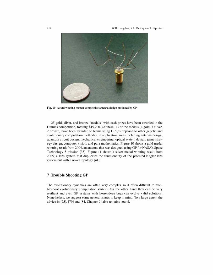
Fig. 10 Award winning human-competitive antenna design produced by GP.
25 gold, silver, and bronze “medals” with cash prizes have been awarded in theHumies competition, totaling $45,700. Of these, 13 of the medals (4 gold, 7 silver,2 bronze) have been awarded to teams using GP (as opposed to other genetic andevolutionary computation methods), in application areas including antenna design,quantum circuit design, mechanical engineering, optical system design, game strat-egy design, computer vision, and pure mathematics. Figure 10 shows a gold medalwinning result from 2004, an antenna that was designed using GP for NASA’s SpaceTechnology 5 mission [35]. Figure 11 shows a silver medal winning result from2005, a lens system that duplicates the functionality of the patented Nagler lenssystem but with a novel topology [41].
7 Trouble Shooting GP
The evolutionary dynamics are often very complex so it often difficult to trou-bleshoot evolutionary computation system. On the other hand they can be veryresilient and even GP systems with horrendous bugs can evolve valid solutions.Nonetheless, we suggest some general issues to keep in mind. To a large extent theadvice in [75], [79] and [84, Chapter 9] also remains sound.
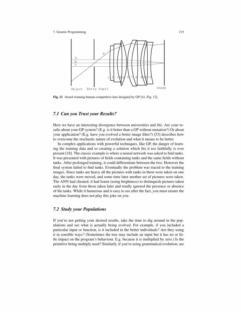
7. Genetic Programming 215
Object Entry Pupil Image
abc
d
1 2 3 4 5 6 7 8 91011 12
Fig. 11 Award winning human-competitive lens designed by GP [41, Fig. 12].
7.1 Can you Trust your Results?
Here we have an interesting divergence between universities and life. Are your re-sults about your GP system? (E.g. is it better than a GP without mutation?) Or aboutyour application? (E.g. have you evolved a better image filter?) [53] describes howto overcome the stochastic nature of evolution and what it means to be better.
In complex applications with powerful techniques, like GP, the danger of learn-ing the training data and so creating a solution which fits it too faithfully is everpresent [18]. The classic example is where a neural network was asked to find tanks.It was presented with pictures of fields containing tanks and the same fields withouttanks. After prolonged training, it could differentiate between the two. However thefinal system failed to find tanks. Eventually the problem was traced to the trainingimages. Since tanks are heavy all the pictures with tanks in them were taken on oneday, the tanks were moved, and some time later another set of pictures were taken.The ANN had cheated, it had learnt (using brightness) to distinquish pictures takenearly in the day from those taken later and totally ignored the presence or absenceof the tanks. While it humerous and is easy to see after the fact, you must ensure themachine learning does not play this joke on you.
7.2 Study your Populations
If you’re not getting your desired results, take the time to dig around in the pop-ulations and see what is actually being evolved. For example, if you included aparticular input or function, is it included in the better individuals? Are they usingit in sensible ways? (Sometimes the tree may include an input but it has no or lit-tle impact on the program’s behaviour. E.g. because it is multiplied by zero.) Is theprimitive being multiply used? Similarly, if you’re using grammatical evolution; are

216 W.B. Langdon, R.I. McKay and L. Spector
your evolved individuals using your grammar as you expected? Or is the grammarbiasing the system in an undesirable or an unexpected way?
Remember GP is doing genetic search. GP increases the numbers of genes (i.e.terminals and functions) which appear in above average fitness individuals. Youmight keep a count of the number of times important primitives occur in the popu-lation. Mostly gene numbers vary randomly according to how lucky they are. How-ever look out for primitives that become extinct or (if using mutation) reduce to lowbackground levels. If this happens, it suggests that the fitness function is driving thecurrent GP population in an unintended direction.
Is the distribution of fitness values of members of the population (particularly thatof the better programs) dominated by a few values with large gaps between them?This suggests jumping these gaps may be hard. It also suggests that the next im-provement may also be separated from the current best. So finding the next improvedsolution will require jumping a large gap and so be difficult. Perhaps changing yourfitness function to be more continuous will improve performance considerably.
7.3 Studying your Programs
A major advantage of GP is you create visible programs. You can see how they work.You can explain how they work to your customers. When presenting GP results, in-clude a slide of the evolved program. The dot package (http://www.graphviz.org/)is good a starting point for nicely presented graphs. GP trees can be automaticallyconverted to dot (http://www.cs.ucl.ac.uk/staff/W.Langdon/lisp2dot.html).
There are methods to automatically simplify expressions (e.g., in Mathematicaand Emacs). However, simply things like removing excess significant digits andcombining constant terms can make your solution more intelligible. After cleaningup the answer, make sure it still works.
In some cases the details of the trees (e.g., the particular nodes) are less importantthan the general size and shape. In [36], Daida describes a way to visualise thesize and shape of either individual trees or an entire population, cf. Figure 12. (AMathematica implementation is available via http://library.wolfram.com/infocenter/MathSource/5163/.)
7.4 Encourage Diversity
If GP is to benefit from using a population: the population must be diverse. (Oth-erwise it might be much more efficient to use a hill climbing or other single pointsearch like simulated annealing.) Sections 7.2 and 7.3 have described measuringits diversity in terms of its genes (i.e. functions and terminals) and the size andshape of the programs. You can also consider the variation in the programs’ be-haviour (c.f., for Boolean problems, [49]). Studying behaviour, as opposed to ge-netic makeup, avoids the problem that GP populations often bloat [53, Sect. 11.3]. In

7. Genetic Programming 217
Fig. 12 The size and shape of 1,000 individuals in the final generation of runs using a depth limitof 50 (on the left) and a size limit of 600 (on the right). The inner circle is at depth 50, and theouter circle is at depth 100. These plots are from [19].
bloated populations syntactically (i.e. genetically) evolved programs appear differ-ent but the difference is in unused code. However studying the programs’ behaviourswill show if the population’s phenotypes have converged excessively.
Since mutation and crossover often produce diverse but low fitness individualsyou could restrict studies of population diversity to just the subset of the populationwhich is selected to have children.
If you suspect the population has converged excessively you could:
• Not use the reproduction operator.• Add one or more mutation operators.• Use a weaker selection mechanism. E.g. reduce the tournament size.• If you are using the “steady state” approach. I.e. you add new programs to the
population immediately, rather than waiting until a whole new population hasbeen created. You could choose who to overwrite at random. (Often people killthe worse member of the population and replace him with the new child. This isfine but tends to increase the convergence of the population.) You might want toprotect the best member of the population to ensure he is not deleted.
• Use a generational population model instead of a steady-state model.• The standard population is panmictic. This means there are no restrictions on
which individual mates with and favourable genetic innovations rapidly spreadthrough and may take over the whole population. In contrast a large populationmay be split into semi-isolated demes [53, Sect. 10.5] which keeps diversity highby slowing the spread of improvements [106, 84].Demes are often used in conjunction with parallel hardware. The speed at whichinnovations spread is controlled both by the number of emigrants and how thedemes are interconnected. Both all-to-all and toroidal topologies are common.They have very short paths between demes. Arranging demes in a ring gives

218 W.B. Langdon, R.I. McKay and L. Spector
a longer convergence time. Typically many individuals (say 2%) are transferedbetween demes each generation. Over Biological timescales, such a high immi-gration rate is sufficient to prevent a converged population diverging into separatespecies. However GP is typically not run for so many generations and, from anengineering standpoint, one has to trade off rapid take up of good solutions versussearching different locations.
• Use fitness sharing or even multi-objective approaches to encourage the forma-tion of many fitness niches.
7.5 Approximate Solutions are Better than No Solution
When GP starts, typically, it starts from nowhere, i.e. well behind the state of the art.For the initial population to evolve, it must contain some programs with an “edge”.With some advantage, even if slight, over the rest of the population. You must de-sign your selection and fitness function to amplify this. A typical fitness functiongives a continuous measure of how far a program is from your requirements. Thefinal program will be a descendent of those you select at the beginning so the fitnessfunction must not only prefer better than random but also reward approximate solu-tion to the whole problem which may be refined into a complete solution. Or rather,an approximate solution to the whole problem.
This is true throughout the run. At every generation the fitness function must seekout approximate solutions from which better ones can be evolved. Even standing stillmay not be enough. Nature tends to the easy thing. In GP this often corresponds tofinding new programs which have the same fitness as their parents. Unfortunatelywithin a few generations, they can evolve to become very resistant to change andfurther progress to your goal (as opposed to theirs) becomes very hard.
Consider (just for illustrative purposes) a problem with just five test cases, fourof which are fairly easy and consequently less important, with the fifth being crucialand quite difficult. So the population may contain individuals that can do the foureasier tasks, but are unable to make the jump to the fifth. There are several things youcould try: 1) weight the hard task more heavily or 2) use a multi-objective approach.However a more fundamental and probably more successful approach is to redesignhow you sort the programs. E.g.: 3) divide the task up in some way into sub-tasks,4) provide more tasks, or 5) change it from being a binary condition (meaning thatan individual does or does not succeed on the fifth task) to a continuous condition,so that an individual GP program can partially succeeds on the fifth task to a greateror less extent. The idea is to create a smoother gradient for the evolutionary processto follow.

7. Genetic Programming 219
7.6 Control Bloat
If you are running out of memory or your execution times seem inordinately long,look the size of your evolved expressions. Often they will be growing over time.It is usually neccessary to provide some form of bloat control, cf. [53, Sect. 11.3].Controlling bloat is also important if one’s goal is to find a comprehensible model,since in practice these must be small. A large model will not only be difficult tounderstand but also may over-fit the training data [55].
7.7 Convince your Customers
For your work to make an impact it must be presented in a form that can convinceothers of the validity of its results and conclusions. This might include: a pitchwithin a corporation seeking continued financial support for a project, the submis-sion of a research paper to a journal or the presentation of a GP-based product topotential customers. [53] contains suggestions on improving written and verbal pre-sentation of artificial evolution experiments. Whilst [56, e.g. Chapter 14] has manysuggestions about getting your work accepted (and paid for) by your customers.
The burden of proof is on the users of GP. It is important to use the customer’slanguage. If the fact that GP discovered a particular chemical is important in a re-action or drug design, you should make this stand out during the presentation. Agreat advantage of GP over many AI techniques in that its results are often sim-ple equations. Ensure these are intelligible to your customer, e.g., by simplification.Also make an effort to present your results using your customer’s terminology. YourGP system may produce answers as trees, but if the customers use spreadsheets,consider translating the tree into a spreadsheet formula.
Also, one should try to discover how the customers intend to validate GP’s an-swer. Do not let them invent some totally new data which has nothing to do with thedata they supplied for training (“just to see how well it does...”). Avoid customerswith contrived data. GP is not omnipotent, it knows nothing about things it has notseen. At the same time you should be scrupulous about your own use of holdoutdata. GP is a very powerful machine learning technique. With this comes the everpresent danger of over-fitting. One should never allow performance on data reservedfor validation to be used to choose which answer to present to the customer.
8 Conclusions
We have seen how genetic programming works and how to use it. We have hintedat just two of the many exciting research areas. The first widens the application ofGP by using formal grammars to capture user knowledge and so guide GP. Thesecond (so far) complementary approach extends GP by doing the opposite! That

220 W.B. Langdon, R.I. McKay and L. Spector
is, sometimes GP can benefit from having additional freedom, including the free-dom to evolve parts of itself. We have skimmed through a few of GP’s many manyapplications, including cases where GP has evolved Human competitive solutions.Finally we have tried to distill some practical “how to” knowledge into a few pages.
To conclude perhaps the best introduction to genetic programming is to createyour own (or borrow someone else’s) and evolve things.
References
1. Alexandros Agapitos and Simon M. Lucas. Learning recursive functions with object orientedgenetic programming. In Pierre Collet et al., eds., EuroGP, LNCS 3905, pp 166–177.
2. Peter J. Angeline. Adaptive and self-adaptive evolutionary computations. In M. Palaniswamiand Y. Attikiouzel, eds., Computational Intelligence: A Dynamic Systems Perspective,pp 152–163. IEEE Press, 1995.
3. Peter J. Angeline. Subtree crossover: Building block engine or macromutation? In J.R. Kozaet al., eds., GP 1997, pp 9–17, Stanford, 13-16 Jul. Morgan Kaufmann.
4. Peter J. Angeline and Jordan Pollack. Evolutionary module acquisition. In D. Fogel andW. Atmar, eds., EP-93, pp 154–163, La Jolla, CA, USA, 25-26 Feb 1993.
5. Yaniv Azaria and Moshe Sipper. GP-gammon: Genetically programming backgammon play-ers. Genetic Programming and Evolvable Machines, 6(3):283–300, 2005.
6. W. Banzhaf. Genotype-phenotype-mapping and neutral variation – A case study in geneticprogramming. In Yuval Davidor et al., eds., PPSN III, LNCS 866, pp 322–332.
7. S. J. Barrett and W. B. Langdon. Advances in the application of machine learning techniquesin drug discovery, design and development. In Ashutosh Tiwari et al., eds., Applications ofSoft Computing: Recent Trends, pp 99–110, 2006 Springer.
8. Franck Binard and Amy Felty. Genetic programming with polymorphic types and higher-order functions. In Maarten Keijzer et al., eds., GECCO ’08:, pp 1187–1194, Atlanta, ACM.
9. Peter A. N. Bosman and Edwin D. de Jong. Grammar transformations in an EDA for geneticprogramming. In R. Poli et al., eds., GECCO 2004 Workshop Proceedings.
10. Valentino Braitenberg. Vehicles. MIT Press, 1984.11. Markus Brameier and Wolfgang Banzhaf. A comparison of linear genetic programming and
neural networks in medical data mining. IEEE Trans. EC, 5(1):17–26, 2001.12. Scott Brave. Evolving recursive programs for tree search. In P.J. Angeline and K. E. Kinnear,
Jr., eds., Advances in Genetic Programming 2, ch 10, pp 203–220. MIT Press, 1996.13. Forrest Briggs and Melissa O’Neill. Functional genetic programming with combinators. In
The Long Pham et al., eds., Proceedings of the Third Asian-Pacific workshop on GeneticProgramming, ASPGP, pp 110–127, Military Technical Academy, Hanoi, VietNam, 2006.
14. W S Bruce. Automatic generation of object-oriented programs using genetic programming.In J.R. Koza et al., eds., GP 1996, pp 267–272, Stanford, 28–31 Jul 1996. MIT Press.
15. Shu-Heng Chen and Chung-Chih Liao. Agent-based computational modeling of the stockprice-volume relation. Information Sciences, 170(1):75–100, 2005.
16. N. Chomsky. Three models for the description of language. IEEE Trans. Information Theory,2(3):113–124, 1956.
17. Rudi Cilibrasi and Paul M. B. Vitanyi. Clustering by compression. IEEE Trans. InformationTheory, 51(4):1523–1545, 2005.
18. David Peter Alfred Corney. Intelligent Analysis of Small Data Sets for Food Design. PhDthesis, University College, London, 2002.
19. Ellery Fussell Crane and N.F. McPhee. The effects of size and depth limits on tree basedgenetic programming. In Tina Yu et al., eds., Genetic Programming Theory and Practice III,ch 15, pp 223–240. Springer, Ann Arbor, 12-14 May 2005.

7. Genetic Programming 221
20. Charles Darwin. Voyage of the Beagle. 1839.21. Charles Darwin. The Origin of Species. John Murray, penguin classics, 1985 edition, 1859.22. Larry Deschaine. Using information fusion, machine learning, and global optimisation to
increase the accuracy of finding and understanding items interest in the subsurface. Geo-Drilling International, 122:30–32, May 2006.
23. Bruce Edmonds. Meta-genetic programming: Co-evolving the operators of variation. CPMReport 98-32, Centre for Policy Modelling, Manchester Metropolitan University, 1998.
24. Brian J. Ross et al. Hyperspectral image analysis using genetic programming. Applied SoftComputing, 5(2):147–156, 2005.
25. C. De Stefano et al. Character preclassification based on genetic programming. PatternRecognition Letters, 23(12):1439–1448, 2002.
26. Christopher J. Neely et al. Is technical analysis in the foreign exchange market profitable? AGP approach. The Journal of Financial and Quantitative Analysis, 32(4):405–426, 1997.
27. Christopher J. Neely et al. The adaptive markets hypothesis: evidence from the foreignexchange market. Working Paper 2006-046B, Federal Reserve Bank of St. Louis, Rev 2007.
28. Conor Ryan et al. Grammatical evolution: Evolving programs for an arbitrary language. InW. Banzhaf et al., eds., EuroGP, LNCS 1391, pp 83–95, Paris, 14-15 Apr 1998.
29. Edward P. K. Tsang et al. EDDIE beats the bookies. Software: Practice and Experience,28(10):1033–1043, 1998.
30. Elsa Jordaan et al. Robust inferential sensors based on ensemble of predictors generated bygenetic programming. In Xin Yao et al., eds., PPSN VIII, LNCS 3242, pp 522–531.
31. Eyal Dassau et al. Modeling and temperature control of rapid thermal processing. Computersand Chemical Engineering, 30(4):686–697, 2006.
32. Friedrich Recknagel et al. Comparative application of artificial neural networks and geneticalgorithms for multivariate time series modelling of algal blooms in freshwater lakes. Hy-droInformatic, 4(2):125–134, 2002.
33. Imran Usman et al. Image authenticity and perceptual optimization via genetic algorithmand a dependence neighborhood. IJAMCS, 4(1):615–620, 2007.
34. Jason H. Moore et al. Symbolic discriminant analysis of microarray data in automimmunedisease. Genetic Epidemiology, 23:57–69, 2002.
35. Jason Lohn et al. Evolutionary antenna design for a NASA spacecraft. In Una-May O’Reillyet al., eds., GPTP II, ch 18, pp 301–315. Springer, Ann Arbor, 13-15 May 2004.
36. J.M. Daida et al. Visualizing tree structures in genetic programming. GP&EM, 6(1):79–110.37. John Paul Marney et al. Risk adjusted returns to technical trading rules: a genetic program-
ming approach. In CEF, Yale, 28-29 Jun 2001.38. J.R. Koza et al. Genetic Programming 3: Darwinian Invention and Problem Solving. Morgan
Kaufman, 1999.39. J.R. Koza et al. Automatic creation of human-competitive programs and controllers by means
of genetic programming. GP&EM, 1(1/2):121–164, 2000.40. J.R. Koza et al. Genetic Programming IV: Routine Human-Competitive Machine Intelli-
gence. Kluwer, 2003.41. J.R. Koza et al. Automated re-invention of six patented optical lens systems using genetic
programming. In Hans-Georg Beyer et al., eds., GECCO 2005, pp 1953–1960.42. Katya Rodriguez-Vazquez et al. Identifying the structure of nonlinear dynamic systems using
multiobjective genetic programming. IEEE Trans. Systems, Man and Cybernetics, Part A,34(4):531–545, 2004.
43. Lee Spector et al. Genetic programming for quantum computers. In J.R. Koza et al., eds.,GP-98, pp 365–373, Madison, Wisconsin, USA, 22-25 Jul 1998. Morgan Kaufmann.
44. Lee Spector et al. Finding a better-than-classical quantum AND/OR algorithm using geneticprogramming. In P.J. Angeline et al., eds., CEC, pp 2239–2246, IEEE Press.
45. Lee Spector et al. The push3 execution stack and the evolution of control. In Hans-Georg Beyer et al., eds., GECCO 2005, pp 1689–1696. ACM Press.
46. Marcos I. Quintana et al. Morphological algorithm design for binary images using geneticprogramming. GP&EM, 7(1):81–102, 2006.

222 W.B. Langdon, R.I. McKay and L. Spector
47. Mark P. Austin et al. Adaptive systems for foreign exchange trading. Quantitative Finance,4(4):37–45, 2004.
48. Nguyen Xuan Hoai et al. Representation and structural difficulty in genetic programming.IEEE Trans. EC, 10(2):157–166, 2006.
49. N.F. McPhee et al. Semantic building blocks in genetic programming. In Michael O’Neill etal., eds., EuroGP 2008, LNCS 4971, pp 134–145, Naples, 26-28 Mar 2008. Springer.
50. Olivier Barriere et al. Modeling human expertise on a cheese ripening industrial processusing GP. In G. Rudolph, editor, PPSN X, LNCS 5199, Dortmund, 13-17 Sep 2008. Springer.
51. Peter Nordin et al. Efficient evolution of machine code for CISC architectures using instruc-tion blocks and homologous crossover. In Lee Spector et al., eds., Advances in GP 3, ch 12,pp 275–299. MIT Press, 1999.
52. Riccardo Poli et al. Smooth uniform crossover, sub-machine code GP and demes: A recipefor solving high-order boolean parity problems. In W. Banzhaf et al., eds., GECCO-99.
53. R. Poli, W.B. Langdon, and N.F. McPhee. A field guide to genetic programming.Published via http://lulu.com and freely available at http://www.gp-field-guide.org.uk, 2008. (With contributions by J. R. Koza).
54. Simon L. Harding et al. Self-modifying cartesian genetic programming. In Dirk Thierens etal., eds., GECCO ’07, pp 1021–1028, London, 7-11 Jul 2007. ACM Press.
55. Sylvain Gelly et al. Universal consistency and bloat in GP. Revue d’Intelligence Artificielle,20(6):805–827, 2006. Issue on New Methods in Machine Learning. Theory and Applications.
56. Tina Yu et al., eds. Evolutionary Computation in Practice. Springer, 2008.57. William Bains et al. Evolutionary computational methods to predict oral bioavailability
QSPRs. Current Opinion in Drug Discovery and Development, 5(1):44–51, 2002.58. Wolfgang Banzhaf et al. Genetic Programming – An Introduction. Morgan Kaufmann, 1998.59. Yin Shan et al. Grammar model-based program evolution. In CEC 2004, pp 478–485.60. James A. Foster. Review: Discipulus: A commercial genetic programming system. GP&EM,
2(2):201–203, 2001.61. Alex Fukunaga. Automated discovery of composite SAT variable selection heuristics. In
AAAI, pp 641–648, 2002.62. Pablo Funes, Elizabeth Sklar, Hugues Juille, and Jordan Pollack. Animal-animat coevolution:
Using the animal population as fitness function. In Rolf Pfeifer et al., eds., SAB, pp 525–533,Zurich, Aug 17-21 1998. MIT Press.
63. D.E. Goldberg. Genetic Algorithms in Search Optimization and Machine Learning. 1989.64. Gilbert Gottlieb. Individual development and evolution: The genesis of novel behavior. Ox-
ford University Press, New York, 1992.65. Frederic Gruau. Genetic micro programming of neural networks. In Kenneth E. Kinnear, Jr.,
editor, Advances in GP, ch 24, pp 495–518. MIT Press, 1994.66. R. J. Hampo and K. A. Marko. Application of genetic programming to control of vehicle
systems. In Proceedings of the Intelligent Vehicles ’92 Symposium, pp 191–195, IEEE.67. Daniel Howard and Simon C. Roberts. Incident detection on highways. In Una-May O’Reilly
et al., eds., GPTP II, ch 16, pp 263–282. Springer, Ann Arbor, 13-15 May 2004.68. Talib S. Hussain and Roger A. Browse. Attribute grammars for genetic representations of
neural networks and syntactic constraints of genetic programming. In Workshop on Evolu-tionary Computation. Held at Canadian Conference on Artificial Intelligence, 1998.
69. Christian Jacob. Genetic L-system programming. In Yuval Davidor et al., eds., PPSN III,LNCS 866, pp 334–343, Jerusalem, 9-14 Oct 1994. Springer.
70. A.K. Joshi, L.S. Levy, and M. Takahashi. Tree adjunct grammars. J. Comput. Syst. Sci.,10:136–163, 1975.
71. Mak Kaboudan. Extended daily exchange rates forecasts using wavelet temporal resolutions.New Mathematics and Natural Computing, 1:79–107, 2005.
72. Douglas Kell. Defence against the flood. Bioinformatics World, pp 16–18, 2002.73. Robert E. Keller and Riccardo Poli. Cost-benefit investigation of a genetic-programming
hyperheuristic. In EA, LNCS 4926, Tours, France, 29-31 Oct 2007. Springer.74. Kenneth E. Kinnear, Jr. Alternatives in automatic function definition: A comparison of per-
formance. In K.E. Kinnear, Jr., editor, Advances in GP, ch 6, pp 119–141. MIT Press, 1994.

7. Genetic Programming 223
75. Kenneth E. Kinnear, Jr. A perspective on the work in this book. In Kenneth E. Kinnear, Jr.,editor, Advances in GP, ch 1, pp 3–19. MIT Press, 1994.
76. Tim J. Klassen and Malcolm I. Heywood. Towards the on-line recognition of arabic charac-ters. In IJCNN’02, pp 1900–1905, 12-17 May 2002. IEEE Press.
77. Arthur Kordon. Evolutionary computation in the chemical industry. In Tina Yu et al., eds.,Evolutionary Computation in Practice, ch 11, pp 245–262. Springer, 2008.
78. Miha Kovacic and Joze Balic. Evolutionary programming of a CNC cutting machine. Inter-national journal for advanced manufacturing technology, 22(1-2):118–124, 2003.
79. John R. Koza. Genetic Programming: On the Programming of Computers by Means ofNatural Selection. MIT Press, 1992.
80. John R. Koza. Genetic Programming II: Automatic Discovery of Reusable Programs. 1994.81. John R. Koza and David Andre. Evolution of iteration in genetic programming. In Lawrence
J. Fogel et al., eds., EP-96, San Diego, Feb 29-Mar 3 1996. MIT Press.82. W. B. Langdon. Global distributed evolution of L-systems fractals. In Maarten Keijzer et al.,
eds., EuroGP’2004, LNCS 3003, pp 349–358, Coimbra, Portugal, 5-7 Apr 2004. Springer.83. W. B. Langdon and B. F. Buxton. Genetic programming for mining DNA chip data from
cancer patients. GP&EM, 5(3):251–257, 2004.84. William B. Langdon. Genetic Programming and Data Structures. Kluwer, 1998.85. William B. Langdon. Size fair and homologous tree genetic programming crossovers.
GP&EM, 1(1/2):95–119, 2000.86. William B. Langdon and Riccardo Poli. Mapping non-conventional extensions of genetic
programming. Natural Computing, 7:21–43, 2008.87. Simon Lucas. Exploiting reflection in object oriented genetic programming. In Maarten Kei-
jzer et al., eds., EuroGP, LNCS 3003, pp 369–378, 5-7 Apr 2004. Springer.88. Penousal Machado and Juan Romero, eds. The Art of Artificial Evolution. Springer, 2008.89. Martin C. Martin. Evolving visual sonar: Depth from monocular images. Pattern Recognition
Letters, 27(11):1174–1180, 2006. Evolutionary Computer Vision and Image Understanding.90. Silja Meyer-nieberg and Hans georg Beyer. Self-adaptation in evolutionary algorithms. In
Parameter Setting in Evolutionary Algorithm. Springer, 2006.91. Julian F. Miller. Evolving developmental programs for adaptation, morphogenesis, and self-
repair. In W. Banzhaf et al., eds., ECAI, LNAI 2801, pp 256–265, 14-17 Sep 2003. Springer.92. Julian F. Miller and Stephen L. Smith. Redundancy and computational efficiency in cartesian
genetic programming. IEEE Trans. EC, 10(2):167–174, 2006.93. David J. Montana. Strongly typed genetic programming. Evolutionary Computation,
3(2):199–230, 1995.94. A. D. Parkins and A. K. Nandi. Genetic programming techniques for hand written digit
recognition. Signal Processing, 84(12):2345–2365, Dec 2004.95. Norman R. Paterson and Mike Livesey. Distinguishing genotype and phenotype in genetic
programming. In John R. Koza, editor, Late Breaking Papers at GP-96, pp 141–150.96. Nelishia Pillay. Evolving solutions to ASCII graphics programming problems in intelligent
programming tutors. In R. Akerkar, ed., International Conference on Applied Artificial Intel-ligence (ICAAI’2003), pp 236–243, Fort Panhala, Kolhapur, India, 15-16 Dec 2003. TMRF.
97. Riccardo Poli. Parallel distributed genetic programming. In David Corne et al., ed., NewIdeas in Optimization, Advanced Topics in Computer Science, chapter 27, pp 403–431.McGraw-Hill, 1999.
98. Alain Ratle and Michele Sebag. Genetic programming and domain knowledge: Beyond thelimitations of grammar-guided machine discovery. In PPSN VI, LNCS 1917, pp 211–220.
99. Alain Ratle and Michele Sebag. Avoiding the bloat with probabilistic grammar-guided ge-netic programming. In P. Collet et al., eds., EA 2001, LNCS 2310, pp 255–266.
100. Craig W. Reynolds. Flocks, herds, and schools: A distributed behavioral model. SIGGRAPHComputer Graphics, 21(4):25–34, 1987.
101. Jurgen Schmidhuber. Evolutionary principles in self-referential learning. on learning nowto learn: The meta-meta-meta...-hook. Diploma thesis, Technische Universitat Munchen,Germany, 14 May 1987.

224 W.B. Langdon, R.I. McKay and L. Spector
102. Lee Spector. Simultaneous evolution of programs and their control structures. In P.J. Ange-line and K. E. Kinnear, Jr., eds., Advances in GP 2, ch 7, pp 137–154. MIT Press, 1996.
103. Lee Spector. Automatic Quantum Computer Programming: A Genetic Programming Ap-proach. Kluwer, 2004.
104. Lee Spector and Adam Alpern. Criticism, culture, and the automatic generation of artworks.In AAAI-94, pp 3–8, Seattle, Washington, USA, 1994. AAAI Press/MIT Press.
105. Lee Spector and H. J. Bernstein. Communication capacities of some quantum gates, discov-ered in part through genetic programming. In Jeffrey H. Shapiro and Osamu Hirota, eds.,QCMC-2003, pp 500–503. Rinton Press, 2003.
106. Lee Spector and Jon Klein. Trivial geography in genetic programming. In Tina Yu et al.,eds., GPTP III, ch 8, pp 109–123. Springer, Ann Arbor, 12-14 May 2005.
107. Lee Spector and Alan Robinson. Genetic programming and autoconstructive evolution withthe push programming language. GP&EM, 3(1):7–40, 2002.
108. Lee Spector and Kilian Stoffel. Ontogenetic programming. In J.R. Koza et al., eds., GP-96,pp 394–399, Stanford, 28–31 Jul 1996. MIT Press.
109. Hideyuki Takagi. Interactive evolutionary computation: Fusion of the capabilities of ECoptimization and human evaluation. Proceedings of the IEEE, 89(9):1275–1296, 2001.
110. Astro Teller. The evolution of mental models. In Kenneth E. Kinnear, Jr., editor, Advancesin GP, ch 9, pp 199–219. MIT Press, 1994.
111. Astro Teller. Evolving programmers: The co-evolution of intelligent recombination opera-tors. In P.J. Angeline and K. E. Kinnear, Jr., eds., Advances in GP 2, pp 45–68. 1996.
112. Ankur Teredesai and Venu Govindaraju. GP-based secondary classifiers. Pattern Recogni-tion, 38(4):505–512, 2005.
113. A. M. Turing. Intelligent machinery. Report for National Physical Laboratory. Reprinted inD.C. Ince, ed. 1992. Mechanical Intelligence: Collected Works of A. M. Turing. 1948.
114. James Alfred Walker and Julian Francis Miller. The automatic acquisition, evolution andreuse of modules in cartesian genetic programming. IEEE Trans. EC 12(4):397–417, 2008.
115. P. A. Whigham and R. I. McKay. Genetic approaches to learning recursive relations. In XinYao, editor, Progress in Evolutionary Computation, LNAI 956, pp 17–27. Springer, 1995.
116. Man Leung Wong and Kwong Sak Leung. Inductive logic programming using genetic algo-rithms. In J. W. Brahan and G. E. Lasker, eds., Advances in Artificial Intelligence - Theoryand Application II, pp 119–124. I.I.A.S., Ontario, Canada, 1994.
117. Man Leung Wong and Kwong Sak Leung. Evolving recursive functions for the even-parityproblem using genetic programming. In P.J. Angeline and K. E. Kinnear, Jr., eds., Advancesin GP 2, ch 11, pp 221–240. MIT Press, 1996.
118. Tina Yu. Hierachical processing for evolving recursive and modular programs using higherorder functions and lambda abstractions. GP&EM, 2(4):345–380, 2001.
119. Tina Yu. A higher-order function approach to evolve recursive programs. In Tina Yu et al.,eds., GPTP III, ch 7, pp 93–108. Springer, Ann Arbor, 12-14 May 2005.
120. Tina Yu and Shu-Heng Chen. Using genetic programming with lambda abstraction to findtechnical trading rules. In Computing in Economics and Finance, 8-10 Jul 2004.
121. Tina Yu and Chris Clack. PolyGP: A polymorphic genetic programming system in haskell.In J.R. Koza et al., eds., GP-98, pp 416–421, 22-25 Jul 1998. Morgan Kaufmann.
122. Mengjie Zhang and Will Smart. Using gaussian distribution to construct fitness functions inGP for multiclass object classification. Pattern Recognition Letters, 27(11):1266–1274.