enzyme genetic programming - heriotml355/common/thesis/michael_lones_thesis.pdf · enzyme genetic...
TRANSCRIPT
Enzyme Genetic ProgrammingModelling Biological Evolvability in Genetic Programming
Michael Adam LonesDepartment of ElectronicsUniversity of York, Heslington, York YO10 5DD
Submitted for the degree of Doctor of Philosophy, September 2003
Thesis committee:
Andy Tyrrell, University of York
Steve Smith, University of York
Keith Downing, Norwegian University of Science and Technology

This thesis is dedicated to all my family and friends.
(So you’d better read it! — I’ll be asking questions!)
2
Abstract
This thesis introduces a new approach to program representation in genetic program-
ming in which interactions between program components are expressed in terms of a
component’s behaviour rather through its relative position within a representation or
through other non-behavioural systems of reference. This approach has the advantage
that a component’s behaviour is expressed in a way that is independent of any par-
ticular program it finds itself within; and thereby overcomes the problem when using
conventional program representations whereby program components lose their be-
havioural context following recombination. More generally, this implicit context rep-
resentation leads to a process of meaningful variation filtering; whereby inappropriate
change induced by variation operators can be wholly or partially ignored. This occurs
as a consequence of program behaviours emerging from the self-organisation of pro-
gram components, ignoring those components which do not fit the contexts declared
by the other components within the program. This process results in gradual change
within the behaviour of a program during evolution. This thesis also presents results
which show that implicit context representation leads to better size evolution charac-
teristics than conventional genetic programming; and that functional redundancy and
Lamarckian reinforcement learning both improve evolutionary search, agreeing with
previous research by other authors.
3

Contents
Acknowledgements 11
Declaration 12
Hypothesis 13
1 Introduction 14
1.1 Genetic Programming . . . . . . . . . . . . . . . . . . . . . . . . . . . . 14
1.2 Biological Modelling . . . . . . . . . . . . . . . . . . . . . . . . . . . . . 15
1.3 Evolvability . . . . . . . . . . . . . . . . . . . . . . . . . . . . . . . . . . 16
1.4 Enzyme Genetic Programming . . . . . . . . . . . . . . . . . . . . . . . 17
1.5 Contributions . . . . . . . . . . . . . . . . . . . . . . . . . . . . . . . . . 17
1.6 Thesis Organisation . . . . . . . . . . . . . . . . . . . . . . . . . . . . . 18
2 Evolution 19
2.1 Evolution of Individuals . . . . . . . . . . . . . . . . . . . . . . . . . . . . 20
2.1.1 Evolvability . . . . . . . . . . . . . . . . . . . . . . . . . . . . . . 21
2.1.2 Evolutionary Spaces and Landscapes . . . . . . . . . . . . . . . 22
2.1.3 Neutral Evolution . . . . . . . . . . . . . . . . . . . . . . . . . . . 23
2.2 Evolution of Groups . . . . . . . . . . . . . . . . . . . . . . . . . . . . . 24
2.2.1 Co-operative Evolution . . . . . . . . . . . . . . . . . . . . . . . . 25
2.2.2 Competitive Evolution . . . . . . . . . . . . . . . . . . . . . . . . 26
2.3 Summary . . . . . . . . . . . . . . . . . . . . . . . . . . . . . . . . . . . 27
2.4 Perspectives . . . . . . . . . . . . . . . . . . . . . . . . . . . . . . . . . 27
4
CONTENTS 5
3 Biological Representation 29
3.1 Biological Components . . . . . . . . . . . . . . . . . . . . . . . . . . . 29
3.1.1 Proteins and Enzymes . . . . . . . . . . . . . . . . . . . . . . . . 29
3.1.2 Nucleic Acids . . . . . . . . . . . . . . . . . . . . . . . . . . . . . 33
3.1.3 Genes . . . . . . . . . . . . . . . . . . . . . . . . . . . . . . . . . 35
3.1.4 Chromosomes . . . . . . . . . . . . . . . . . . . . . . . . . . . . 39
3.1.5 Cells . . . . . . . . . . . . . . . . . . . . . . . . . . . . . . . . . . 41
3.2 Biological Processes . . . . . . . . . . . . . . . . . . . . . . . . . . . . . 42
3.2.1 DNA Replication . . . . . . . . . . . . . . . . . . . . . . . . . . . 42
3.2.2 Transcription . . . . . . . . . . . . . . . . . . . . . . . . . . . . . 45
3.2.3 Cell Division . . . . . . . . . . . . . . . . . . . . . . . . . . . . . 49
4 Biochemical Pathways 54
4.1 Metabolic Networks . . . . . . . . . . . . . . . . . . . . . . . . . . . . . 54
4.2 Signalling Networks . . . . . . . . . . . . . . . . . . . . . . . . . . . . . 57
4.3 Gene Expression . . . . . . . . . . . . . . . . . . . . . . . . . . . . . . . 60
5 Biological Evolvability 63
5.1 Compartmentalisation . . . . . . . . . . . . . . . . . . . . . . . . . . . . 64
5.2 Redundancy . . . . . . . . . . . . . . . . . . . . . . . . . . . . . . . . . 66
5.2.1 Functional redundancy . . . . . . . . . . . . . . . . . . . . . . . 66
5.2.2 Structural redundancy . . . . . . . . . . . . . . . . . . . . . . . . 67
5.2.3 Weak Linkage . . . . . . . . . . . . . . . . . . . . . . . . . . . . 67
5.3 Evolution through Redundancy . . . . . . . . . . . . . . . . . . . . . . . 68
5.4 Neutral Evolution . . . . . . . . . . . . . . . . . . . . . . . . . . . . . . . 69
5.5 Other Sources of Evolvability . . . . . . . . . . . . . . . . . . . . . . . . 72
5.6 Evolution of Evolvability . . . . . . . . . . . . . . . . . . . . . . . . . . . 73
5.7 Summary . . . . . . . . . . . . . . . . . . . . . . . . . . . . . . . . . . . 74
6 Genetic Programming 75
6.1 Evolutionary Computation . . . . . . . . . . . . . . . . . . . . . . . . . . 75
6.1.1 Genetic Algorithms . . . . . . . . . . . . . . . . . . . . . . . . . . 77
6.2 Conventional Genetic Programming . . . . . . . . . . . . . . . . . . . . 78
6.3 Problems with Recombination . . . . . . . . . . . . . . . . . . . . . . . . 80
CONTENTS 6
6.4 Solution Size Evolution and Bloat . . . . . . . . . . . . . . . . . . . . . . 82
6.5 Expressiveness . . . . . . . . . . . . . . . . . . . . . . . . . . . . . . . . 84
6.5.1 Linguistic Approaches . . . . . . . . . . . . . . . . . . . . . . . . 85
6.5.2 Representational Approaches . . . . . . . . . . . . . . . . . . . . 90
6.6 Summary . . . . . . . . . . . . . . . . . . . . . . . . . . . . . . . . . . . 94
7 Evolvability in Evolutionary Computation 95
7.1 Variation versus Representation . . . . . . . . . . . . . . . . . . . . . . 95
7.2 Adapting Variation . . . . . . . . . . . . . . . . . . . . . . . . . . . . . . 96
7.3 Introducing Pleiotropy . . . . . . . . . . . . . . . . . . . . . . . . . . . . 97
7.3.1 Modularity . . . . . . . . . . . . . . . . . . . . . . . . . . . . . . . 98
7.3.2 Implicit Reuse . . . . . . . . . . . . . . . . . . . . . . . . . . . . 101
7.4 Evolvability through Redundancy . . . . . . . . . . . . . . . . . . . . . . 102
7.4.1 Structural Redundancy . . . . . . . . . . . . . . . . . . . . . . . 102
7.4.2 Coding Redundancy and Neutrality . . . . . . . . . . . . . . . . . 106
7.4.3 Functional Redundancy . . . . . . . . . . . . . . . . . . . . . . . 109
7.5 Positional Independence . . . . . . . . . . . . . . . . . . . . . . . . . . . 114
7.5.1 Linkage Learning . . . . . . . . . . . . . . . . . . . . . . . . . . . 114
7.5.2 Floating Representations . . . . . . . . . . . . . . . . . . . . . . 115
7.5.3 Gene Expression . . . . . . . . . . . . . . . . . . . . . . . . . . . 117
7.6 Summary . . . . . . . . . . . . . . . . . . . . . . . . . . . . . . . . . . . 118
7.7 Perspectives . . . . . . . . . . . . . . . . . . . . . . . . . . . . . . . . . 119
8 Enzyme Genetic Programming 121
8.1 Introduction . . . . . . . . . . . . . . . . . . . . . . . . . . . . . . . . . . 121
8.2 Representing Programs in Genetic Programming . . . . . . . . . . . . . 122
8.2.1 Explicit context . . . . . . . . . . . . . . . . . . . . . . . . . . . . 123
8.2.2 Indirect context . . . . . . . . . . . . . . . . . . . . . . . . . . . . 124
8.3 Implicit Context Representation . . . . . . . . . . . . . . . . . . . . . . . 125
8.3.1 An Illustrative Example . . . . . . . . . . . . . . . . . . . . . . . 126
8.3.2 Representing Programs with Implicit Context . . . . . . . . . . . 128
8.4 Implicit Context in Enzyme Genetic Programming . . . . . . . . . . . . . 129
8.4.1 Functionality . . . . . . . . . . . . . . . . . . . . . . . . . . . . . 130
8.5 Program Development . . . . . . . . . . . . . . . . . . . . . . . . . . . . 133
CONTENTS 7
8.6 Evolution of Program Representations . . . . . . . . . . . . . . . . . . . 136
8.6.1 Initialisation and Variation . . . . . . . . . . . . . . . . . . . . . . 137
8.7 Summary . . . . . . . . . . . . . . . . . . . . . . . . . . . . . . . . . . . 140
9 Experimental Results and Analysis 141
9.1 Experimental Method . . . . . . . . . . . . . . . . . . . . . . . . . . . . 141
9.1.1 Symbolic Regression . . . . . . . . . . . . . . . . . . . . . . . . 142
9.2 Comparative Performance . . . . . . . . . . . . . . . . . . . . . . . . . . 144
9.3 Functionality . . . . . . . . . . . . . . . . . . . . . . . . . . . . . . . . . 146
9.4 Recombinative Behaviour . . . . . . . . . . . . . . . . . . . . . . . . . . 147
9.4.1 Effect of crossover type . . . . . . . . . . . . . . . . . . . . . . . 147
9.4.2 Crossover versus Mutation . . . . . . . . . . . . . . . . . . . . . 149
9.4.3 Microscopic Behaviours . . . . . . . . . . . . . . . . . . . . . . . 150
9.5 Size Evolution . . . . . . . . . . . . . . . . . . . . . . . . . . . . . . . . . 153
9.6 Redundancy . . . . . . . . . . . . . . . . . . . . . . . . . . . . . . . . . 156
9.7 Phenotypic Linkage . . . . . . . . . . . . . . . . . . . . . . . . . . . . . 158
9.7.1 Phenotypic Linkage Learning . . . . . . . . . . . . . . . . . . . . 160
9.7.2 Stability and Replication Fidelity . . . . . . . . . . . . . . . . . . 161
9.8 Genetic Linkage . . . . . . . . . . . . . . . . . . . . . . . . . . . . . . . 163
9.9 Component Reuse . . . . . . . . . . . . . . . . . . . . . . . . . . . . . . 164
9.10 Development . . . . . . . . . . . . . . . . . . . . . . . . . . . . . . . . . 166
9.11 Discussion . . . . . . . . . . . . . . . . . . . . . . . . . . . . . . . . . . 167
10 Summary and Conclusions 174
10.1 Rationale and Work Done . . . . . . . . . . . . . . . . . . . . . . . . . . 174
10.2 Conclusions . . . . . . . . . . . . . . . . . . . . . . . . . . . . . . . . . . 178
10.3 Limitations of This Study . . . . . . . . . . . . . . . . . . . . . . . . . . . 181
10.4 Further Work . . . . . . . . . . . . . . . . . . . . . . . . . . . . . . . . . 182
A The Activity Model 187
List of Tables
7.1 An example redundant code . . . . . . . . . . . . . . . . . . . . . . . . . . . . . . 108
9.1 Metrics used to measure performance and behaviour of program evolution. . . . 142
9.2 Behavioural parameters and their default settings. . . . . . . . . . . . . . . . . . 143
9.3 Boolean regression test problems. . . . . . . . . . . . . . . . . . . . . . . . . . . 144
9.4 Performance of enzyme GP with different operators . . . . . . . . . . . . . . . . 144
A.1 Performance of activity model upon two-bit multiplier problem. . . . . . . . . . . . 187
8

List of Figures
2.1 An evolutionary system . . . . . . . . . . . . . . . . . . . . . . . . . . . . . . . . 20
2.2 Evolution of a group of entities . . . . . . . . . . . . . . . . . . . . . . . . . . . . 24
2.3 Co-operative interactions during evolution . . . . . . . . . . . . . . . . . . . . . . 26
3.1 Hierarchical levels of protein structure . . . . . . . . . . . . . . . . . . . . . . . . 30
3.2 Enzyme activity . . . . . . . . . . . . . . . . . . . . . . . . . . . . . . . . . . . . . 32
3.3 Nucleotides of DNA . . . . . . . . . . . . . . . . . . . . . . . . . . . . . . . . . . 34
3.4 DNA Replication . . . . . . . . . . . . . . . . . . . . . . . . . . . . . . . . . . . . 43
3.5 Protein synthesis through transcription and translation . . . . . . . . . . . . . . . 45
3.6 Mitotic cell division . . . . . . . . . . . . . . . . . . . . . . . . . . . . . . . . . . . 50
3.7 Meiosis . . . . . . . . . . . . . . . . . . . . . . . . . . . . . . . . . . . . . . . . . 51
4.1 Biochemical Pathways . . . . . . . . . . . . . . . . . . . . . . . . . . . . . . . . . 55
4.2 The citrate cycle . . . . . . . . . . . . . . . . . . . . . . . . . . . . . . . . . . . . 56
4.3 Initiation of a Signalling Pathway . . . . . . . . . . . . . . . . . . . . . . . . . . . 59
6.1 One generation of an evolutionary algorithm . . . . . . . . . . . . . . . . . . . . . 76
6.2 Sub-tree crossover . . . . . . . . . . . . . . . . . . . . . . . . . . . . . . . . . . . 79
6.3 Loss of context following sub-tree crossover . . . . . . . . . . . . . . . . . . . . . 81
6.4 Grammatical evolution . . . . . . . . . . . . . . . . . . . . . . . . . . . . . . . . . 89
7.1 Koza’s branch creation operator . . . . . . . . . . . . . . . . . . . . . . . . . . . . 99
7.2 A GP expression tree containing introns . . . . . . . . . . . . . . . . . . . . . . . 105
7.3 Cartesian GP circuit with functional redundancy . . . . . . . . . . . . . . . . . . . 112
7.4 Recombination in Harik’s Linkage Learning GA . . . . . . . . . . . . . . . . . . . 116
8.1 Mapping from program representation to program . . . . . . . . . . . . . . . . . . 122
8.2 Loss of context during cartesian GP recombination . . . . . . . . . . . . . . . . . 124
8.3 Evolution of an abstract implicit context system . . . . . . . . . . . . . . . . . . . 127
9
LIST OF FIGURES 10
8.4 Enzyme model . . . . . . . . . . . . . . . . . . . . . . . . . . . . . . . . . . . . . 130
8.5 Example functionality space . . . . . . . . . . . . . . . . . . . . . . . . . . . . . . 131
8.6 Derivation of functionality . . . . . . . . . . . . . . . . . . . . . . . . . . . . . . . 133
8.7 Format of a program representation . . . . . . . . . . . . . . . . . . . . . . . . . 134
8.8 Top-down development of a simple Boolean expression . . . . . . . . . . . . . . 135
8.9 An example of strongest-first development . . . . . . . . . . . . . . . . . . . . . . 136
8.10 Structure of the network genetic algorithm . . . . . . . . . . . . . . . . . . . . . . 137
8.11 A conceptual view of enzyme GP uniform crossover . . . . . . . . . . . . . . . . 139
8.12 Recombination using transfer and remove . . . . . . . . . . . . . . . . . . . . . . 139
9.1 The two-bit multiplier problem . . . . . . . . . . . . . . . . . . . . . . . . . . . . . 143
9.2 Comparing functionality shapes and random shapes . . . . . . . . . . . . . . . . 145
9.3 Effect of shape calculation upon performance . . . . . . . . . . . . . . . . . . . . 146
9.4 Comparing uniform and TR recombination . . . . . . . . . . . . . . . . . . . . . . 147
9.5 Headless chicken recombination . . . . . . . . . . . . . . . . . . . . . . . . . . . 148
9.6 Comparing relative abilities of recombination and mutation operators . . . . . . . 150
9.7 A simple example of subsumption . . . . . . . . . . . . . . . . . . . . . . . . . . 151
9.8 Behaviours resulting from transfer and remove operations. . . . . . . . . . . . . . 152
9.9 Two-bit multiplier size evolution . . . . . . . . . . . . . . . . . . . . . . . . . . . . 154
9.10 Effect of transfer limit upon size evolution . . . . . . . . . . . . . . . . . . . . . . 155
9.11 Evolution of program size . . . . . . . . . . . . . . . . . . . . . . . . . . . . . . . 156
9.12 Comparing program size growth against forced representation growth . . . . . . 157
9.13 Effect of removing non-coding components . . . . . . . . . . . . . . . . . . . . . 158
9.14 Effect of number of binding sites upon performance . . . . . . . . . . . . . . . . . 158
9.15 Evolution of phenotypic linkage . . . . . . . . . . . . . . . . . . . . . . . . . . . . 159
9.16 Relationship between phenotypic linkage and representation length . . . . . . . 160
9.17 Performance of phenotypic linkage learning . . . . . . . . . . . . . . . . . . . . . 161
9.18 Effects of phenotypic linkage learning . . . . . . . . . . . . . . . . . . . . . . . . 162
9.19 Effect of size of function and input terminal sets . . . . . . . . . . . . . . . . . . . 163
9.20 Evolution of genetic linkage and relationship with representation length . . . . . 164
9.21 Functional component reuse . . . . . . . . . . . . . . . . . . . . . . . . . . . . . 165
9.22 Behaviour of development strategies . . . . . . . . . . . . . . . . . . . . . . . . . 166
9.23 Scalability of development strategies . . . . . . . . . . . . . . . . . . . . . . . . . 167
10.1 Variation filtering preserves output behaviour . . . . . . . . . . . . . . . . . . . . 180
10.2 Implicit structural context . . . . . . . . . . . . . . . . . . . . . . . . . . . . . . . . 183
A.1 Visualising the activity model . . . . . . . . . . . . . . . . . . . . . . . . . . . . . 188
A.2 Evolution of a full adder with the activity model . . . . . . . . . . . . . . . . . . . 189

Acknowledgements
I would particularly like to thank my parents for all their love and support; Andy
Tyrrell, for all the advice, pastoral care and beer he has provided my with during the
long years of my doctorate; Paul, for all the support, for being a great friend, and for
being my drinking partner; Austin, for keeping me down to earth, keeping me laugh-
ing, and plying me with beer; Alex, for his comradeship, encyclopædic brain, and
strong coffee; Andy Greenboy, fellow research gimp, provider of tea, and mainstay of
the Buzzard massive; Becky and Rosie, for sleeping on me, for letting me stroke them,
and for all the dead shrews they faithfully bring to me; and last, but never least, Elise;
for her friendship, for keeping me entertained, and for teaching me to find solace in
my work.
I would also like to offer special thanks to all my colleagues at York, past and present,
for their help and friendship; to Steve Smith and Keith Downing, my examiners, for
their constructive advice; and to Spike the goose and his feathered friends, for being
there when I needed someone to talk to.
11

Declaration
Some of the research presented in this thesis has previously been published by the au-
thor [Lones and Tyrrell, 2001c,b,a, 2002b,a, 2003b,a]. All work presented in this thesis
as original is so to the best knowledge of the author. References and acknowledge-
ments to other researchers have been given as appropriate.
12
Hypothesis
This research follows from the notion that models of biological representations can
be used within genetic programming to represent executable structures; motivated by
the expectation that these models will capture useful biological properties that will
improve the evolution of executable structures. More specifically, it is asserted that:
• Representations from engineering domains are not designed to respond to ran-
dom change in a meaningful way. In genetic programming, this is demonstrated
by the poor response of conventional representations towards recombination op-
erators.
• Biological representations are a product of evolution and are therefore well adap-
ted for representing evolving artefacts. In particular, they are believed to confer
evolvability — the capacity to exhibit change in an appropriate direction — to
the artefacts that they represent.
• Many biological structures are known to carry out activities of a computational
nature. This includes metabolic, signalling, gene expression and neural path-
ways. It has also been shown that models of these structures can be used to
represent non-biological computational artefacts.
Following from these assertions, it is hypothesised that models of biological repre-
sentations can be used to represent computer programs and other artificial executable
structures within genetic programming, thereby improving the evolvability of these
structures.
13
1 Introduction
1.1 Genetic Programming
Genetic programming (GP) is an evolutionary computation approach to automatic
programming; designing programs to solve a particular task through the use of an
algorithm modelled upon processes and mechanisms of biological evolution. Ge-
netic programming has several apparent advantages over better known automatic
programming techniques. Unlike formal methods, GP requires no knowledge about
the problem that it is attempting to solve other than a measure of how good a solu-
tion is, and once a GP run has been initiated it requires no human interaction. Unlike
inductive logic programming, GP does not attempt to carry out an exhaustive search
of the problem’s solution space; but rather exploits its search history to identify those
areas which are more likely to contain global optima.
However, GP is far from perfect. For much of its execution, it fails to effectively ex-
ploit its search history: since its model of biological recombination does not, on the
whole, produce better programs from existing programs. GP has a bloat problem: the
programs that it generates tend to become larger and larger at a rate which rises in line
with a quadratic function; filling up the available space and making it near-impossible
to find small, efficient solutions. Like other evolutionary computation approaches, GP
has a scalability problem: increasing problem size leads to an unmanageably high
increase in space and time resource requirements.
Nevertheless, the GP approach is not futile. It is still a young field of research, it is
attracting a growing research community, and there are many avenues of research yet
to be explored. Moreover, it already shows a lot of promise. GP has been used to
14
1 Introduction 15
solve a huge variety of problems: from designing robot controllers to discovering new
quantum algorithms to understanding the role of genetic motifs and protein structures
in biology. One of its particular strengths is its ability to find solutions to problems
which a human would probably never consider: making it possible to solve problems
in fields which humans do not thoroughly understand (like biology); or find hard to
understand (like quantum computing); and to discover new, more efficient solutions
to problems which humans have already solved (such as computer algorithms); not to
mention its ability to inform humans through reverse-engineering of these solutions.
1.2 Biological Modelling
Modelling biology on computers has been a prevailing theme for much of the history
of computation. It is the ambition of many computer scientists to create computers
which are as powerful and flexible as animal brains. Accordingly, it is logical to draw
information from systems which have already achieved this feat: biological systems.
Nevertheless, the interests of computer scientists in biology are not limited to neural
processes. Biological systems have many properties which are the envy of computer
science; for example: growth, learning, reconfigurability, self-repair, fault tolerance,
and reproduction — though of course there are many biological processes, mecha-
nisms and artefacts which at the moment would have no conceivable benefit within
the silicon environment of a computer.
Biological modelling gave birth to evolutionary computation, yet there are mixed
views within the EC community regarding biological modelling within evolutionary
computation. A number of researchers cite the ‘No Free Lunch’ theory [Wolpert and
Macready, 1995] whilst warning against the futility of introducing greater complex-
ity to evolutionary algorithms: yet this same theory also predicts that evolutionary
computation can be no better than random search across the whole spectrum of prob-
lem domains. Clearly, EC is considerably better than random search upon the kinds
of problems that computer scientists actually want to solve. Other researchers have
championed the value of biological modelling within EC; testifying to the obvious
superiority of biological evolution over simulated evolution.
1 Introduction 16
1.3 Evolvability
Evolvability is the relative capacity for something to exhibit appropriate change. For a
biological organism, evolvability is the relative likelihood that random genetic change
could lead to an improvement in the organism’s fitness. For computer software, evolv-
ability is the ease with which new functionality can be introduced by a human pro-
grammer. For a human language, evolvability is a measure of its ability to express
new concepts and accept new constructs and methods of communication as required.
These examples illustrate that evolvability is meaningful within many domains. In
fact, the concept of evolvability can be thought of as a pattern which can be applied to
any domain where an entity or group of entities is subject to a process of change; and
particularly where a domain has some notion of a particular direction of change being
more valuable than another.
What is perhaps less appreciated is that concepts of how to achieve evolvability can
also be applied across domains. For example, in software systems modularity is seen
as a source of evolvability since it limits the effect of change to a local region of the
program. This limits the global impact of change within the program, making it easier
to apply change, and making it less likely that any errors will propagate to other parts
of the program. Likewise, biological organisms develop in a compartmental fashion,
allowing individual compartments to be evolved separately and making it less likely
that genetic errors will propagate within the whole organism [Conrad, 1990].
The work reported in this thesis is motivated to a large degree by the premise that
principles of biological evolvability can be applied within non-biological artefacts in
order to improve the way in which they evolve. This premise is motivated by a num-
ber of observations: (i) the way in which biological organisms are represented is be-
lieved to be a product of evolution and therefore presumably superior to many other
potential representations; (ii) these representations are evidently capable of describing
and supporting the evolution of highly complex systems i.e. biological organisms; (iii)
these representations are capable of describing systems of computation; and (iv) many
principles of evolvability are known to be applicable across domains. That biological
representations can describe computation is perhaps not obvious but is supported by
the developing community of computer scientists who use models of biological pro-
cesses to carry out information processing and other overtly computational tasks.
1 Introduction 17
1.4 Enzyme Genetic Programming
The product of this work is a GP system called enzyme genetic programming. En-
zyme genetic programming has many similarities with conventional GP systems: in
that it uses a population based evolutionary algorithm; it applies recombination and
mutation operators to create new programs; it specifies a problem using a fitness func-
tion, a function set and a terminal set; and it generates programs represented by parse
trees. However, it does not use parse trees to represent programs during evolution but
rather uses a new program representation modelled upon the way in which enzyme
systems are represented in biology. The consequences of this new representation for
evolution are examined at length in the pages to come.
1.5 Contributions
This work makes the following principle contributions to knowledge:
• The development and understanding of a new implicit context form of program
representation in which program components interact through behavioural de-
scriptions rather than through relative positions or arbitrary references.
• The implementation of a genetic programming system based upon an implicit
context representation, showing how this new form of representation may be
used in practice.
• The development of the concept of meaningful variation filtering, whereby a
representation can filter out the effects of inappropriate variation events whilst
promoting meaningful change.
• The demonstration that implicit context representation leads to meaningful pro-
gram recombination as a result of meaningful variation filtering.
• The realisation that functional redundancy within an implicit context representa-
tion is structured as a subsumption hierarchy and supports meaningful variation
filtering through the action of variation operators upon this structure.
1 Introduction 18
1.6 Thesis Organisation
This thesis is organised into three main segments. Chapters 1 to 5 introduce the con-
cepts of biological representation, evolution, and evolvability. Chapters 6 and 7 review
related work in genetic programming and evolutionary computation. Chapters 8 to
10 describe the novel contributions of this research. Specifically:
Chapter 1 is this introduction.
Chapter 2 introduces evolution; describing how evolution can be understood as a
general process which exhibits common behaviours across domains.
Chapter 3 reviews the fundamental components of biological representation.
Chapter 4 discusses how these components are organised into higher-level structures.
Chapter 5 introduces the concept of evolvability and discusses the sources of evolv-
ability within biological systems.
Chapter 6 reviews fundamental topics in genetic programming: focussing on its lim-
itations and derivative approaches.
Chapter 7 reviews approaches to improving the evolvability of evolutionary compu-
tation, placing particular emphasis upon genetic programming and the role of
biological modelling.
Chapter 8 introduces enzyme genetic programming; discussing the motivation be-
hind the approach and its implementation.
Chapter 9 presents experimental analysis of enzyme genetic programming, discusses
the experimental results, and identifies key evolutionary behaviours.
Chapter 10 summarises, draws conclusions, and offers some speculative suggestions
for future research.
Appendix A describes the activity model, an approach which predates the current
version of enzyme genetic programming.
2 Evolution
Evolution is a process that leads to change. In particular domains, the term evolution
is used to refer to specific processes of change. In the study of social development, for
instance, evolution is used to describe the development of societies. In mathematics,
evolution is an iterative process which finds the root of a number. Stellar evolution, in
astronomy, is the process of star formation. Software evolution, in software engineer-
ing, is the change in functionality over the lifetime of a software system. Biological
evolution is the change in genetic constitution of a population of organisms over time.
Even in Darwin’s era, there was nothing new about the idea of evolution. Evolution
has been acting, and could easily be seen to be acting, in myriad systems since the
dawn of history. The thing that shocked Victorian people was the idea that biologi-
cal populations, too, were subject to evolution and therefore not entirely shaped by
the will of God — or, to take the ‘theory of evolution’ [Darwin, 1859] to its ultimate
conclusion, formed entirely by a process of selection acting upon essentially random
variation.
This chapter has several objectives. First, to introduce the properties of a range of
example evolutionary systems. Second, to present commonalities that exist between
the properties of these systems and establish a general view of evolutionary systems.
Third, to develop a standard taxonomy and terminology of evolutionary systems.
Above all, the aim of this chapter is to demonstrate that it is possible to introduce the
key concepts of evolution without having to talk about biological evolution: and, in
this way, show that ideas concerning evolution have relevance to a broader range of
domains than biology alone.
19
2 Evolution 20
Representation
Entity
Representation’
Entity’
Variation
Evolution
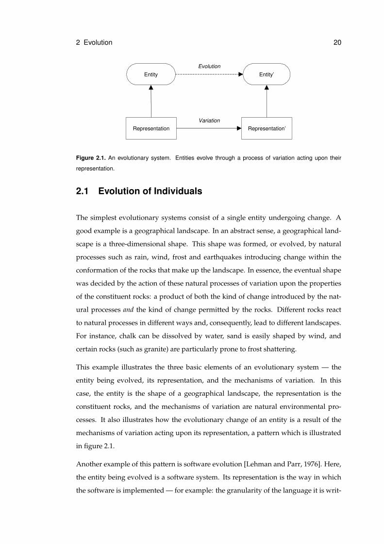
Figure 2.1. An evolutionary system. Entities evolve through a process of variation acting upon their
representation.
2.1 Evolution of Individuals
The simplest evolutionary systems consist of a single entity undergoing change. A
good example is a geographical landscape. In an abstract sense, a geographical land-
scape is a three-dimensional shape. This shape was formed, or evolved, by natural
processes such as rain, wind, frost and earthquakes introducing change within the
conformation of the rocks that make up the landscape. In essence, the eventual shape
was decided by the action of these natural processes of variation upon the properties
of the constituent rocks: a product of both the kind of change introduced by the nat-
ural processes and the kind of change permitted by the rocks. Different rocks react
to natural processes in different ways and, consequently, lead to different landscapes.
For instance, chalk can be dissolved by water, sand is easily shaped by wind, and
certain rocks (such as granite) are particularly prone to frost shattering.
This example illustrates the three basic elements of an evolutionary system — the
entity being evolved, its representation, and the mechanisms of variation. In this
case, the entity is the shape of a geographical landscape, the representation is the
constituent rocks, and the mechanisms of variation are natural environmental pro-
cesses. It also illustrates how the evolutionary change of an entity is a result of the
mechanisms of variation acting upon its representation, a pattern which is illustrated
in figure 2.1.
Another example of this pattern is software evolution [Lehman and Parr, 1976]. Here,
the entity being evolved is a software system. Its representation is the way in which
the software is implemented — for example: the granularity of the language it is writ-
2 Evolution 21
ten in, its internal structure of decomposition, its choice of data structures and algo-
rithms. The mechanism of variation is the programmer or programmers responsible
for maintaining and updating the code. Again, it is the action of the mechanism of
variation (the programmers) upon the representation (the implementation) that de-
cides how the software system evolves.
However, this example has a significant difference to the previous example: evolution
is directed. In geographical landscapes, evolution is the consequence of rocks anneal-
ing to environmental processes. There is no external pressure for the system to evolve
in any particular direction. In software systems, on the other hand, evolution in the di-
rection of increased functionality is the objective of the programmers who modify the
implementation. Consequently, programmers introduce variation that they believe
will increase the functionality of the software system. This directed variation leads to
directed evolution.
2.1.1 Evolvability
Evolvability [Conrad, 1990, Kirschner and Gerhart, 1998, Nehaniv, 2003] is a measure
of an evolutionary system’s ability to evolve in an appropriate direction. To re-iterate
a point made earlier, the evolution of an entity is a consequence of the mechanisms
of variation inducing change within the entity’s representation: a result of both the
mechanisms of variation’s ability to express change and the representation’s ability to
accept change. Accordingly, the evolvability of an evolutionary system is a function
of both the evolvability accorded by the entity’s representation and the evolvability
accorded by the mechanisms of variation.
In the context of the software evolution example, this entails that the degree to which
the evolution of a software system can be directed is a function of not only the pro-
grammers’ ability to conduct appropriate change but also the implementation’s ca-
pacity to accept appropriate change. This is not to say that any programmer could
not make an appropriate change to the functionality of any existing software system
given enough time and energy, but rather that certain approaches to implementation
(those which accord greater evolvability) accept these changes more easily than others
and that certain forms of code maintenance (those which accord greater evolvability)
generate these changes more easily than others.
2 Evolution 22
In this example, the evolvability accorded by an implementation could be measured
by the number of lines of code which have to be added or changed in order to produce
the desired functionality. An implementation accords evolvability if it is designed in
such a way that a minor change in functionality can be achieved with a minor change
in its code. An implementation does not accord evolvability if a minor change in
functionality can only be achieved through a major re-write of its code. This prin-
ciple is widely recognised within software engineering where programmers are en-
couraged to write code in such a way that functionality can be adapted with minimal
code change. Mechanisms to achieve this include abstraction, which achieves robust-
ness through functional redundancy; modularisation, which limits the propagation of
code changes; and re-use, which removes the need to duplicate changes.
An interesting property of software systems (which is also true of biological systems)
is that these architectural mechanisms are recorded within the code of the implementa-
tion alongside the code which implements the software’s functionality. Consequently,
when programmers modify code they are targeting both functional and architectural
components of the representation. Therefore, for programmers who maintain soft-
ware to do so in a way that accords evolvability, they must make appropriate changes
to both functional and architectural components of the representation. Again (al-
though to a lesser degree) this principle is recognised within software engineering and
programmers are encouraged to modify code in a way that both implements the re-
quired changes in functionality and preserves, or improves, the evolvability accorded
by the implementation. Mechanisms such as code re-factoring exist to help program-
mers achieve this.
2.1.2 Evolutionary Spaces and Landscapes
When talking about evolution, it is often useful to visualise the evolutionary process
as movement within an abstract space of all possible conformations of the evolving
entity or its representation. It is also conventional, though not always appropriate,
to organise these spaces so that neighbouring points represent entities that differ by
an amount equivalent to the change introduced by a single variation event; although
since there are often multiple sources of variation, this is usually only meaningful if a
separate space is envisaged for each source of variation. Nevertheless, such spaces are
2 Evolution 23
useful for measuring the evolvability of an evolutionary system since, by measuring
the distance between the locations of different entities, it can be seen how much effort
will be required to evolve one entity into another.
Within some evolutionary systems it is convenient to assign values of worth to each
possible conformation of an evolving entity. For example, within a software system
undergoing evolution, each possible version of the software can be given a value that
reflects how likely it is to sell within the software marketplace. For such evolutionary
systems it is useful to extend the notion of evolutionary space by giving each point a
value which reflects its worth: in effect, adding another dimension. Since points close
together within the evolutionary space refer to similar entities with typically similar
values of worth, this augmented space tends to have what looks like a continuous
hyper-surface in the value dimension with peaks in regions of high value entities and
valleys in regions of low value entities. In analogy to this appearance, these spaces are
often referred to as landscapes [Conrad, 1979, Jones, 1995].
Evolution is often described as a search process. Nevertheless, for most evolutionary
systems evolution does not lead to behaviours which would be normally be thought
of as search (although you could describe evolution as searching for the natural bi-
ases caused by an entity’s representation and mechanisms of variation). However,
certain evolutionary systems do carry out search behaviours and often this search can
be described as directed movement within an evolutionary landscape: moving from a
location corresponding to a low valued solution to a location corresponding to a high
valued solution.
2.1.3 Neutral Evolution
Sometimes when the representation of an entity experiences variation, the entity itself
does not change. This is called neutral evolution [Kimura, 1983]. It occurs when there is
a one-to-many mapping between entity and representation: such that a single entity
can be described by many representations. Neutral evolution is the result of variation
switching between members of this set of equivalent representations.
Returning to the real-world example of a software system, a typical neutral evolution
event would involve turning a piece of code into a function and replacing its original
2 Evolution 24
Entities
Group
Entities’
Group’
Variation
Evolution
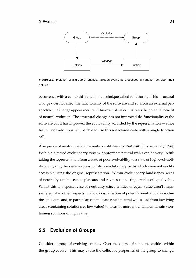
Figure 2.2. Evolution of a group of entities. Groups evolve as processes of variation act upon their
entities.
occurrence with a call to this function, a technique called re-factoring. This structural
change does not affect the functionality of the software and so, from an external per-
spective, the change appears neutral. This example also illustrates the potential benefit
of neutral evolution. The structural change has not improved the functionality of the
software but it has improved the evolvability accorded by the representation — since
future code additions will be able to use this re-factored code with a single function
call.
A sequence of neutral variation events constitutes a neutral walk [Huynen et al., 1996].
Within a directed evolutionary system, appropriate neutral walks can be very useful:
taking the representation from a state of poor evolvability to a state of high evolvabil-
ity, and giving the system access to future evolutionary paths which were not readily
accessible using the original representation. Within evolutionary landscapes, areas
of neutrality can be seen as plateaus and ravines connecting entities of equal value.
Whilst this is a special case of neutrality (since entities of equal value aren’t neces-
sarily equal in other respects) it allows visualisation of potential neutral walks within
the landscape and, in particular, can indicate which neutral walks lead from low-lying
areas (containing solutions of low value) to areas of more mountainous terrain (con-
taining solutions of high value).
2.2 Evolution of Groups
Consider a group of evolving entities. Over the course of time, the entities within
the group evolve. This may cause the collective properties of the group to change:
2 Evolution 25
causing, in effect, an evolutionary process at the group level. This process of group
evolution, shown in figure 2.2, obeys the same pattern as the evolution of individual
entities (shown in figure 2.1) whereby evolution occurs as a consequence of mecha-
nisms of variation acting upon a representation — but in this case, the representation
is the entities that comprise the group.
As an example, consider a group of software systems, each of which has limited func-
tionality. Over time, the developers of the software systems will modify their imple-
mentations in order to improve their functionality. Consequently, the level of function-
ality of the group will appear to evolve in a positive direction. If there is a tendency
for developers to develop certain kinds of functionality, perhaps in response to mar-
ket demands, then the type of functionality of the group will appear to evolve in a
particular direction. If developers choose their objectives non-deterministically, then
the functionality of the group will tend to become increasingly diverse. The evolution
of these collective properties is a result of variation acting upon the entities within the
group.
2.2.1 Co-operative Evolution
Exchange of information — or more generally, interaction — between members of
a group can alter the dynamics of the group-level evolutionary process. This is of
particular interest within groups undergoing directed evolution, where the direction
(and speed) of evolution is highly dependent upon the nature of interaction between
members of the group.
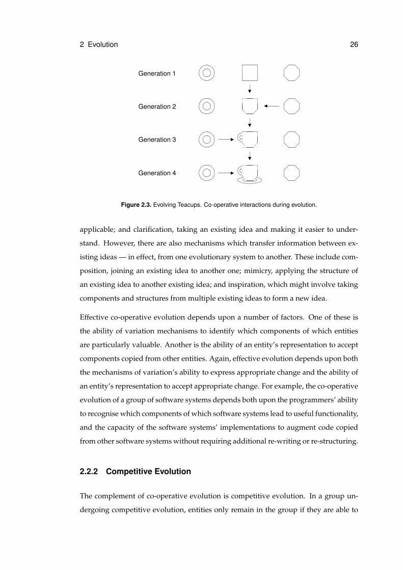
Co-operative evolution occurs when entities within a group share information about
how to increase their value. Co-operation works via mechanisms of variation which
attempt to identify valuable components of entities and copy these components into
other entities. The effect of co-operative evolution is to improve the collective search
capacity of the group above that of a group of non-interacting evolving entities. Figure
2.3 shows a simple example of co-operative evolution.
A good example of co-operative evolution is the evolution of ideas [Dawkins, 1976].
Ideas evolve via variation produced by the mechanisms of human thought. These
mechanisms include generalisation, taking an existing idea and making it more widely
2 Evolution 26
Generation 1
Generation 2
Generation 3
Generation 4
Figure 2.3. Evolving Teacups. Co-operative interactions during evolution.
applicable; and clarification, taking an existing idea and making it easier to under-
stand. However, there are also mechanisms which transfer information between ex-
isting ideas — in effect, from one evolutionary system to another. These include com-
position, joining an existing idea to another one; mimicry, applying the structure of
an existing idea to another existing idea; and inspiration, which might involve taking
components and structures from multiple existing ideas to form a new idea.
Effective co-operative evolution depends upon a number of factors. One of these is
the ability of variation mechanisms to identify which components of which entities
are particularly valuable. Another is the ability of an entity’s representation to accept
components copied from other entities. Again, effective evolution depends upon both
the mechanisms of variation’s ability to express appropriate change and the ability of
an entity’s representation to accept appropriate change. For example, the co-operative
evolution of a group of software systems depends both upon the programmers’ ability
to recognise which components of which software systems lead to useful functionality,
and the capacity of the software systems’ implementations to augment code copied
from other software systems without requiring additional re-writing or re-structuring.
2.2.2 Competitive Evolution
The complement of co-operative evolution is competitive evolution. In a group un-
dergoing competitive evolution, entities only remain in the group if they are able to
2 Evolution 27
compete effectively against the other entities in the group. As a consequence, the aver-
age ability of entities to compete will tend to increase over time as those entities which
compete poorly are removed. Competition may occur either as a result of competitive
interactions within the group or as a result of some external selective mechanism. In
a software marketplace, for example, competition between software systems is deter-
mined by customer preferences. Those which are preferred by customers will survive
and continue to be evolved; those which are not preferred by customers may be dis-
continued and removed from the marketplace. Accordingly, the average quality of
software systems will tend to increase over time.
2.3 Summary
Evolution is a process which leads to change within an entity or group of entities over
a period of time. Evolution results from some process or processes of variation acting
upon the representation of an entity or group of entities. Importantly, an entity can
undergo a certain evolutionary change if and only if this change is possible as a re-
sult of processes of change acting upon the entity’s representation. Evolvability is the
capacity for an evolutionary system to evolve in a particular direction; and is deter-
mined by the nature of the entity, by the flexibility of the entity’s representation, and
by the ability of the variation operators to induce appropriate change. Directed evolu-
tion, which can lead to evolution carrying out a process of search, can be encouraged
within groups of entities through both co-operative and competitive mechanisms.
2.4 Perspectives
The interest of the scientific and engineering communities in developing a unified
view of evolution is a recent phenomenon [Nehaniv, 2003]. Nevertheless, there is con-
siderable commonality between the evolutionary processes which occur in different
kinds of system: and a growing view that lessons learnt from one evolutionary do-
main can be applied within other evolutionary domains. The issue of evolvability
is particularly relevant; since an understanding of evolvability is essential in under-
standing how best to design and represent artefacts — such as software systems and
2 Evolution 28
engineered products — which are subject to a process of change over time. Evolv-
ability is also of paramount importance within evolutionary computation systems. In
the past, the choices of representation within evolutionary computation have been
somewhat arbitrary from an evolvability perspective. Typically an evolutionary com-
putation practitioner will use the form of representation which is most natural or most
common for a given entity; without thinking about whether or not it is evolvable. In
part this is due to a lack of understanding regarding what is and what is not evolv-
able. This thesis presents a biologically motivated approach to the development of an
evolvable representation for evolutionary computation: an approach motivated by the
relatively large amount of information concerning evolvability which may be mined
from biological systems. However, this is not the only approach, and it is conceivable
that other, perhaps equally fruitful approaches, could be developed by looking at how
evolution occurs in a much broader range of both natural and artificial systems.
3 Biological Representation
The functioning of biological systems can be described at many levels from the in-
teractions between individual biochemicals up through interactions at increasingly
higher levels of organisation: biochemical pathways, organelles, cells, tissues, organs,
organisms, populations, species, communities and ecosystems; and interactions with
the abiotic environment including, for some species, cultural artefacts.
This chapter aims to show how functionality is represented at a low level within bi-
ological systems. It is divided into two sections. The first section describes the low-
level components from which biological systems are constructed. The second section
describes the processes by which these components are constructed and replicated.
Unless otherwise indicated, this material can be found in biological textbooks such as
Lodish et al. [2003], Brown and Brown [2002], and Lewin [2000].
3.1 Biological Components
3.1.1 Proteins and Enzymes
Proteins are the main functional element of the body and play a role within almost ev-
ery biological process. Specified by a sequence of amino acids, each species of protein
has a unique three dimensional structure. It is this structure which determines the
protein’s effect upon other biological elements and, accordingly, its function within
the biological system.
Amino acids are a group of molecules unified by a common structure. Of the many
possible amino acids, only twenty varieties are normally found in biological systems.
29
3 Biological Representation 30
H C COOH
NH 2
R
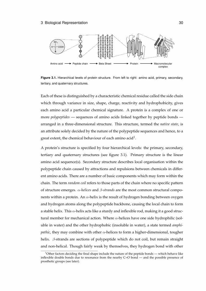
Amino acid Peptide chain Beta Sheet Protein Macromolecular complex
Figure 3.1. Hierarchical levels of protein structure. From left to right: amino acid, primary, secondary,
tertiary, and quaternary structures.
Each of these is distinguished by a characteristic chemical residue called the side chain
which through variance in size, shape, charge, reactivity and hydrophobicity, gives
each amino acid a particular chemical signature. A protein is a complex of one or
more polypeptides — sequences of amino acids linked together by peptide bonds —
arranged in a three-dimensional structure. This structure, termed the native state, is
an attribute solely decided by the nature of the polypeptide sequences and hence, to a
great extent, the chemical behaviour of each amino acid1.
A protein’s structure is specified by four hierarchical levels: the primary, secondary,
tertiary and quaternary structures (see figure 3.1). Primary structure is the linear
amino acid sequence(s). Secondary structure describes local organisation within the
polypeptide chain caused by attractions and repulsions between chemicals in differ-
ent amino acids. There are a number of basic components which may form within the
chain. The term random coil refers to those parts of the chain where no specific pattern
of structure emerges. α-helices and β-strands are the most common structural compo-
nents within a protein. An α-helix is the result of hydrogen bonding between oxygen
and hydrogen atoms along the polypeptide backbone, causing the local chain to form
a stable helix. This α-helix acts like a sturdy and inflexible rod, making it a good struc-
tural member for mechanical action. Where α-helices have one side hydrophilic (sol-
uble in water) and the other hydrophobic (insoluble in water), a state termed amphi-
pathic, they may combine with other α-helices to form a higher-dimensional, tougher
helix. β-strands are sections of polypeptide which do not coil, but remain straight
and non-helical. Though fairly weak by themselves, they hydrogen bond with other
1Other factors deciding the final shape include the nature of the peptide bonds — which behave likeinflexible double bonds due to resonance from the nearby C=O bond — and the possible presence ofprosthetic groups (see later).
3 Biological Representation 31
β-strands (running parallel or anti-parallel) to form β-sheets. The presence of amino
acid residues on both sides of the sheet can allow for interesting behaviours to emerge
— for instance if those on one side are hydrophilic and the other side hydrophobic.
Tougher structures result when sheets form stacks.
Turns, composed of three or four amino acids, are sharp bends in the chain resulting
from hydrogen bonding between the residues at either end of the sequence. Motifs
are distinctive combinations of secondary structures, with characteristic function and
primary structure. An example is the zinc finger, a motif consisting of one α-helix
and two β-strands. These form a cage around a single zinc atom; the assembled motif
resembling, and offering similar function to, a finger. The zinc atom involved in this
motif is an example of a prosthetic group — a tightly bound non-peptide molecule or
metal which provides structural support, a binding site, or some other function to the
protein.
Tertiary structure defines the folded form of the protein when introduced to an aque-
ous environment — where hydrophobic interactions pull the secondary structure into
a more compact form. Typically, the protein will configure itself into a number of
distinct regions, called structural domains, which encompass a section of the polypep-
tide chain containing numerous secondary structures. A cluster of structural domains
which together provide a localised function within the protein are deemed a func-
tional domain. Functional domains which recur in many proteins (and therefore exist
as building blocks) are known as tertiary domains.
Where a protein consists of more than one polypeptide, a final layer of structure —
quaternary structure — describes the positioning of polypeptide subunits. In certain
circumstances, multiple proteins may form an aggregate structure. These are called
macromolecular assemblies.
Enzymes
Enzymes are proteins which act to catalyse other chemical reactions. For a chemical
reaction to take place, an activation energy must be met. Usually, this is provided
by the kinetic energy of the reactants. However, for many reactions, the kinetic en-
ergy required is substantial and is only available at hot temperatures. In biological
3 Biological Representation 32
������� ������ �� ����������� ��� �� � ������������� � ����������������� �������
substratesproducttransition-state�
intermediateallosteric�inhibition
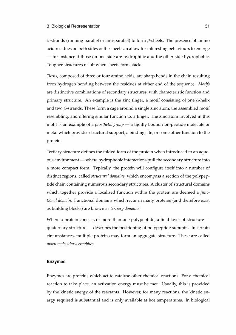
Figure 3.2. Enzyme activity
systems, ambient temperature is relatively low, making most reactions energetically
unfavourable. To make these reactions possible, either the activation energy must be
met — not usually possible — or it must be lowered. This is the function of enzymes
(see figure 3.2). Enzymes possess specificity, an ability to recognise2 only certain chem-
icals and bind exclusively to these. The chemicals recognised, the substrates, are the
reactants needed for the reaction. By bringing these together, the kinetic energy re-
quired for the reaction to occur is reduced, and hence the activation energy of the
reaction is lowered.
Most important reactions do not take place immediately. Rather, the reaction pro-
gresses through a number of transition states. During this process, the substrates are
converted through a series of transition-state intermediates until, after the final tran-
sition stage, they become the reaction’s final products. For an enzyme to effectively
catalyse a reaction, it must not only bind to substrates, but also to transition-state in-
termediates.
Binding of substrates occurs at active sites on the enzyme. Active sites are produced
by a precise arrangement of amino acid residues which, when in contact, bond non-
covalently with complementary sites on the substrate’s surface. This is called the lock-
and-key mechanism. Recognition of a substrate may also cause structural change in
the enzyme, induced fit, which brings the substrate into closer contact with the active
site. Non-covalent bonding holds the substrate in place. However, the enzyme may
also form covalent bonds with a substrate. It is these bonds which change the nature
2Recognition here, and elsewhere in molecular systems, refers to a stable non-covalent bonding be-tween large macromolecules — a result of diffusion rather than active convergence.
3 Biological Representation 33
of the substrate, converting it into a transition-state intermediate. Subsequent changes
in the substrate occur either by contact with other reactants, or by further enzymatic
action (making and breaking of covalent bonds). In order for the correct bonds to be
made, amino acid residues alone may be insufficient. In these circumstances, pros-
thetic groups may be used. Prosthetic groups used in this way are called co-enzymes.
Since chemical reactions require energy and resources, for purposes of efficiency it
is desirable that reactions only take place as and when they are required. Conse-
quently, the function of enzymes are regulated so that reactions are only catalysed
when the current chemical conditions make them useful. This is achieved through
effector-binding sites which, when bound, either inhibit or activate the enzyme. The
molecules which bind to these sites are called effectors. In the case where the (inhibit-
ing) effector is the product of the reaction which the enzyme catalyses, this is called
feedback inhibition. Moreover, in real biological systems, products of reactions often
become reactants of other reactions. In these cases, the product of the final reaction
may be the effector of the enzyme involved in the first reaction. Hence, this enzyme
will only become functional when the end product is in short supply and, in effect,
the entire pipeline will be disabled at other times (since the first reaction produces
the reactants for the second, and so on). Inhibition and activation occur through con-
formational change induced by bonding at the effector site. This change of shape for
purposes of regulation is called allostery.
3.1.2 Nucleic Acids
While proteins provide the functional elements of a biological system, it is nucleic
acids which specify and aid construction of these units. These roles are provided, re-
spectively, by deoxyribonucleic acid (DNA) and ribonucleic acid (RNA), both of which are
polyesters composed of nucleotides. Nucleotides, like amino acids, are small molecules
with common structure, differentiated between by side groups. These side groups are
called bases, and are of two types — purines and pyramidines. Purines are substantially
larger than pyramidines. The purines found in biological systems are Adenine and
Guanine, each identified by their initial letters, A and G. The pyramidines are Cyto-
sine (C), Thymine (T) and Uracil (U). Nucleotides with Thymine bases are only found
in DNA and those with Uracil are found only in RNA. Nucleotides are formed when
3 Biological Representation 34
C
C
C
N
C
N
N
N
HC
H
H
N
H
H
O
N
C
C
C
C
N
H
H
H
O
NH2
N
C
C
C
C
N
H3C
H
H
O
O
H
C
C
C
N
C
N
N
N
CH
H
H
NH2
� �"!$#&% #(' )+*(,.-"/�% #('
021 '$#&% #(' 354�*�67% #('
A T
G C
C G
A T
C G
A
C A
TA
CG
AT
GC
A
GC
AT
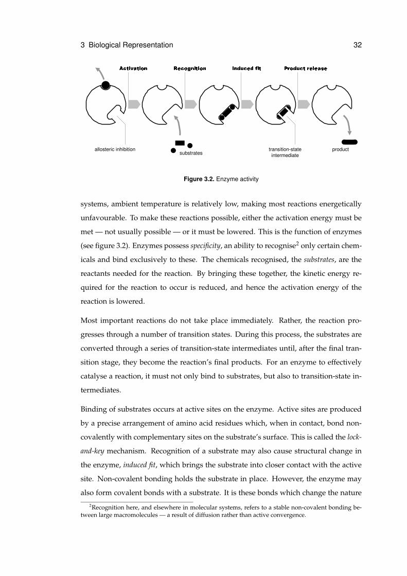
Figure 3.3. Nucleotides of DNA
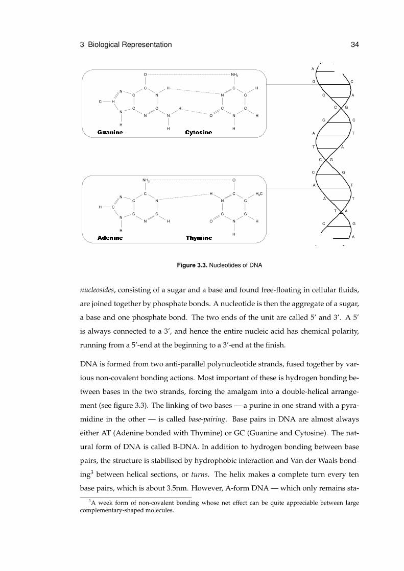
nucleosides, consisting of a sugar and a base and found free-floating in cellular fluids,
are joined together by phosphate bonds. A nucleotide is then the aggregate of a sugar,
a base and one phosphate bond. The two ends of the unit are called 5’ and 3’. A 5’
is always connected to a 3’, and hence the entire nucleic acid has chemical polarity,
running from a 5’-end at the beginning to a 3’-end at the finish.
DNA is formed from two anti-parallel polynucleotide strands, fused together by var-
ious non-covalent bonding actions. Most important of these is hydrogen bonding be-
tween bases in the two strands, forcing the amalgam into a double-helical arrange-
ment (see figure 3.3). The linking of two bases — a purine in one strand with a pyra-
midine in the other — is called base-pairing. Base pairs in DNA are almost always
either AT (Adenine bonded with Thymine) or GC (Guanine and Cytosine). The nat-
ural form of DNA is called B-DNA. In addition to hydrogen bonding between base
pairs, the structure is stabilised by hydrophobic interaction and Van der Waals bond-
ing3 between helical sections, or turns. The helix makes a complete turn every ten
base pairs, which is about 3.5nm. However, A-form DNA — which only remains sta-
3A week form of non-covalent bonding whose net effect can be quite appreciable between largecomplementary-shaped molecules.
3 Biological Representation 35
ble in non-aqueous environments — turns every eleven base pairs. This is a more
compact form of DNA, with a turn of about 2.3nm, but only occurs when DNA is re-
moved from solution. Both A- and B-DNA are right-handed varieties. A further form,
Z-DNA, is left-handed, but has never been observed in natural biological systems.
DNA in eukaryotes, such as animals and plants, is found in linear form. However,
in prokaryotes and viruses DNA is circular, with the 5’-end attached to the 3’-end.
Sometimes sections of circular DNA may become underwound. This state is energeti-
cally unfavourable, and so the entire strand is pulled towards a more favourable state
— either by reducing the overall twist or by forming supercoils (where the degree of
supercoiling is measured as writhe).
DNA is an information store, a purpose to which it is well-suited due to its relative
long-life and stability. RNA sacrifices long-life for lability; a fact reflected in its mul-
titude of uses within biological systems. It can occur in single-stranded and double-
stranded varieties, linear or circular, can hybridise with DNA, and can combine with
proteins to form ribonucleoprotein complexes. Like proteins, RNA can form three-
dimensional structures: allowing expression of catalytic and auto-catalytic behaviours
(for instance, breaking and splicing other RNA molecules). These structures are de-
scribed by three levels of organisation. Primary structure describes the base sequence,
secondary specifies two-dimensional structure such as loops and hairpins, and ter-
tiary describes interacting two-dimensional features which form three-dimensional
structures such as pseudoknots.
The purpose of DNA in biological systems is to store a description of the organism
in which the DNA is found. This information, called the genome, is expressed by a
language written in the genetic code — the alphabet of bases found in DNA — namely,
A, C, G and T. However, this information is not a blueprint, but rather a highly decen-
tralised developmental plan which describes, by specifying systems of proteins, how
the organism will function at a local level. The overall nature of the organism is then
emergent from the sum of these local functions.
3.1.3 Genes
According to Mendel [1965], the founder of genetic science, a gene is a unit of inher-
itance, a ‘particulate factor that passes unchanged from parent to progeny’. From a
3 Biological Representation 36
functional viewpoint, a gene is a stretch of polypeptide chain encoding one protein,
or more exactly, a fragment of DNA which can be transcribed by messenger RNA.
Although the language and chemical structure of prokaryotic and eukaryotic DNAs
are virtually the same, there are two major differences in genetic structure. The first
of these concerns the unit of transcription. In prokaryotes, it is normal for several
genes to be encompassed by the same transcription unit. This means that a single
mRNA can encode several different proteins, each of which can be synthesised inde-
pendently by a ribosome. In eukaryotes, by contrast, ribosomes may only begin syn-
thesis at the beginning of an mRNA strand, entailing that eukaryotic mRNA may only
transcribe from a single gene. This is called monocistronic RNA. Prokaryotic mRNA is
polycistronic. The cluster of genes from which this is transcribed is an operon — with
transcription starting from a short stretch of DNA called a promoter. If this promoter
is mutated, then all the genes in the operon may become non-functional, a fact which
makes prokaryotic DNA less fault-tolerant than its eukaryotic cousin. However, this
approach is slightly more efficient than having many separate transcription and syn-
thesis events — and efficiency is very important to a prokaryote, where evolutionary
pressure selects against any waste of energy. Moreover, low-level efficiency is rel-
atively unimportant to a eukaryotic organism, for which behavioural effectiveness is
the dominant evolutionary selector. This, too, explains the second major difference be-
tween prokaryotic and eukaryotic DNA. Prokaryotic DNA is tightly packed, with al-
most all the polypeptide used to encode functional genes. By comparison, eukaryotic
DNA consists mostly of non-coding DNA, the relative quantity of which varies widely
between species and does not correlate with the size or complexity of the organism.
Eukaryotic genes consist of exons, coding segments, and introns, non-coding segments.
During transcription, both coding and non-coding parts are copied to mRNA. Before
protein synthesis, mRNA excises its non-coding introns to form a continuous stretch
of coding RNA.
Solitary genes are genes which occur only once in the genome, accounting for between
twenty-five and fifty percent of all genes. A gene family is a set of nearby4 genes which
encode similar, but not identical, amino acid sequences (a protein family). Polypep-
tide sequences which are similar to genes but are non-functional are called pseudo-
4This proximity suggests that similar genes may be a result of unequal crossover — crossover betweenchromosomes which are not properly aligned.

3 Biological Representation 37
genes. Quite often, sequences of bases occur over and over again in a repeated array.
Depending on whether the sequence is a gene or is non-coding, these are called either
tandemly repeated genes or repetitious DNA fragments. Tandemly repeated genes encode
proteins for which demand is greater than that which can possibly be transcribed from
a single gene in a given time period. To meet demand, transcription of many identical
genes occurs in parallel.
More generally, there are three classes of eukaryotic DNA. These are identified, and
named, according to how fast they re-associate after their strands have been sepa-
rated. Where there are tandem arrays of short sequences (5–10 base pairs), sections
of one strand can bond to many sections on the other, pulling the strands together
very quickly. Such DNA is called rapid reassociation rate, or simple sequence, DNA. Due
to the way it forms bands around other DNA when centrifuged, it is also known as
satellite DNA. Regions of fewer repeats are minisatellites, with small differences in the
length of minisatellites between members of the same species providing the basis for
genetic fingerprinting. A single variety of simple sequence DNA can occupy up to one
percent of the genome in total, and is often found in specific areas of the chromosome.
Intermediate reassociation rate, or intermediate repeat, DNA represents many occurrences
of larger base sequences. Compared to simple sequence DNA, there are relatively few
varieties of these, although each variety occurs in large numbers. Repeating sequences
of between 150 and 300 base pairs are classed as short interspersed elements, SINES,
whereas those of 5000 to 7000 base pairs are LINES, long interspersed elements. In-
termediate repeat DNA is either found in large tandem arrays (e.g. functional gene
tandem arrays) or scattered randomly around the genome. This latter class includes
mobile DNA elements — DNA sequences that are able to move or copy themselves
to other regions of DNA. These sequences, which have no real purpose other than
self-replication5, occupy about thirty percent of the human genome. Slow reassocia-
tion rate DNA, or single copy DNA, occupies between fifty and sixty percent of the
genome. Of this, only five percent encodes genes — the rest being spacer DNA with
mostly no known function.
Although seen as a molecular parasite, using the organism’s transcription facility
without giving anything in return, mobile DNA is thought to have evolutionary sig-5Which gives mobile DNA the alternative name of selfish DNA. This should not be confused with
Dawkins’ [1976] idea of the selfish gene, which is unrelated.
3 Biological Representation 38
nificance. On the whole, transposition of mobile DNA is balanced by mutation, which
destroys existing copies with no disadvantage to the organism. However, it does lead
to variance in the lengths of chromosomes — meaning that it is possible that two chro-
mosomes of unequal length will be crossed over. The result of this is unequal crossover,
which can lead to duplication and mutation of existing genes. Mobile DNA can also
carry with it parts of genes it has overwritten. If these parts are then copied into other
genes when the mobile DNA moves, exon shuffling takes place — the creation of novel
genes from combinations of pre-existing exons [Gilbert, 1978].
There are two broad classes of mobile DNA, categorised by their transposition mech-
anism. Transposons remain as DNA throughout the move. They are either excised or
copied from their original location and then inserted at their new location. Retrotrans-
posons transpose via an RNA intermediate, and hence are always copied rather than
moved. RNA polymerase encodes the retrotransposon as RNA. An enzyme called
reverse transcripterase then copies this to a new segment of DNA which is then in-
serted into the chromosome. Retrotransposons are either viral or non-viral, with viral
retrotransposons encoding a viral shell which, when synthesised, allows the retro-
transposon to leave the cell and infect other cells and organisms. Non-viral retro-
transposons are either LINES or SINES. LINES encode reverse transcripterase. SINES,
however, use the reverse transcripterase synthesised by LINES, meaning they can be
much shorter (in effect, they are hyperparasites).
Prokaryotes also contain selfish DNA. In bacteria, insertion sequences (IS elements)
are 1.5kb segments of single-strand DNA which invade normal double stranded DNA
(homoduplex), forming a heteroduplex with one strand containing the extra IS element.
Insertion sequences include instructions for synthesising transposase, which allows
the IS element to move within the bacterial DNA. However, since bacterial DNA is
tightly packed, these moves are likely to generate fatal mutations. For this reason,
surviving IS elements transpose very rarely.
The introduction of new, useful, genes as well as occasional beneficial effects of mu-
tation and exon shuffling are rare chance events. The role of mobile DNA is, on the
whole, non-functional. By contrast, local cellular processes sometimes carry out rear-
rangements of DNA with a specific functional intent. These include inversion of DNA
sequences, gene conversion, amplification and segment deletion. The role of inversion
3 Biological Representation 39
is varied, and depends upon the organism. For instance, in the bacterium salmonella,
it is used to alter the expression of certain surface proteins. Once the host organism has
produced antibodies for the primary infection, bacteria which experience this inver-
sion will not be recognised, producing a secondary infection for the body to combat.
Gene conversion results in a component of an active gene being updated with an inac-
tive part from elsewhere in the chromosome, changing the protein produced by the
gene. The uses of this mechanism, again, are varied. Gene amplification, also called
polytenation, causes parts of chromosomes to be replicated. The replicants are either
than released, or remain connected. This is the mechanism used to produce lots of
copies of the rRNA gene. It is a dynamic alternative to tandem arrays. Finally, segment
deletion is involved in the separation and rearrangment of segments of DNA, allowing
many forms to be generated from a set of DNA segments (e.g. antibodies).
3.1.4 Chromosomes
In many organisms, genomic DNA is arranged into chromosomes. Dividing the ge-
nome into storage units in this manner makes the large amount of data easier to store
and handle. However, the genome is very large. In its natural form, even split into
sub-units, the DNA is far too voluminous to fit into a single cell, let alone a nucleus. In
prokaryotes, which have relatively small genomes, the natural random coil formed by
the single circular chromosome would be one thousand times larger than a bacterial
cell. Much of this expanse is due to electric charge repulsion between the negatively
charged phosphate groups in the DNA backbone. The prokaryotic solution to this
problem is to introduce positively charged polyamine groups, which associate with
the phosphate groups to shield the charges. Additionally, numerous small proteins
bind to the DNA, folding it into a more compact structure, and finally, special enzymes
induce supercoiling.
The eukaryotic solution to the compaction problem is called chromatin, a complex of
DNA and structural proteins. These proteins, H1, H2A, H2B, H3 and H4 are all mem-
bers of the histone family and retain a high degree of similarity between species. Two
each of H2A, H2B, H3 and H4 form a histone octomer, a roughly cylindrical shaped
object that acts like a reel around which DNA can be wound. A nucleosome is a histone
octomer with slighty less than two windings of DNA (146 bases). This is the primary
3 Biological Representation 40
structural unit of chromatin. Further organisation produces a solenoid form, euchro-
matin, with six nucleosomes per turn. This structure is stabilised by an association of
histone H1 with each nucleosome — forming chromatosomes. During interphase (the
period between cell divisions), euchromatin is the normal level of chromosome struc-
ture, the non-condensed form of chromatin. During metaphase (cell division), when
chromosomes become visible to the light microscope, the chromosome experiences
several degrees of supercoiling, forming a compact structure called heterochromatin,
the condensed form. This is supported by an internal scaffold6 of non-histone pro-
teins. The number, size and shape of heterochromatin complexes during metaphase is
an organism’s karyotype. During interphase, some sections of the chromosome remain
as heterochromatin, occuring in regions where no transcription takes place. When in-
terphase chromosomes are stained by certain dyes, these regions of heterochromatin
form dark bands. Staining of metaphase chromosomes also produces characteristic
bands. However, the cause of this banding is unknown, yet provides a useful roadmap
within the organism’s karyotype.
Most sequences of bases in DNA are either protein encoding genes or non-coding
redundant regions. However, other sequences are designed with a functional role.
These have arrangements of bases which are recognised by various types of binding
proteins, such as transcription sites. Three such regions are of particular importance
for chromosome duplication and segregation — autonomously replicating sequences
(ARSs), the centromere and the telomeres. ARSs are origins of replication. These
are bound to by special proteins which start the replication process. Centromeres
have binding sequences for proteins which hold and follow the microtubule spindle.
Telomeres7 protect the ends of chromosomes, and are placed after replication. They
also provide a binding point outside of the main chromosome where replication of the
chromosome ends can occur from. Otherwise, it would not be possible to replicate the
last few bases of a linear chromosome, creating shorter chromosomes each generation.
6During interphase, chromosomes remain associated with this scaffold. Binding sites between thechromosome and scaffold are called scaffold-associated regions (SAR’s), occuring between transcriptionregions. During transcription, the solenoid in the transcription region unwinds to allow access by tran-scription proteins.
7Telomeres consist entirely of guanine bases, forming a loop at the end of the chromosome. The sidesof the loop are bound together by non Watson-Crick G-G bonds.
3 Biological Representation 41
3.1.5 Cells
Cells are the fundamental unit of most biological systems (or the unit, in the case of
some). It is local processing done by cells which, when combined with communica-
tion between cells, lead to the emergent behaviour of a single organism. This local
processing, called the metabolism, is in turn the sum of all chemical processes which
occur within the cell.
Within the biological community, the prevailing view is of a single heritage to all cells.
However, from the current standpoint in evolution, cells can be seen as falling into two
broad categories — prokaryotic and eukaryotic. Organisms which consist of these types
of cell are called, respectively, prokaryotes and eukaryotes. Prokaryotes encompass
the most primitive organisms on Earth, the bacteria. This cell lineage can be further
divided into eubacteria and archaebacteria, the latter of which is considered by some
as a separate lineage to the prokaryotes. Eubacteria are common, and consequently
well studied. Archaebacteria live in unusual environments such as swamps and sul-
phur springs, and at the cellular level have many features in common with eukaryotes.
Eukaryotes include animals, plants and fungi.
Both prokaryotic and euakaryotic cells are contained within a plasma membrane. The
plasma membrane is a semi-permeable layer which maintains the integrity of its con-
tents by controlling inward and outward movement of chemicals. Prokaryotic cells are
fairly unstructured. Eukaryotic cells, however, contain extensive internal membranes
which organise the cell into compartments of local metabolic processing, organelles.
The largest of these, and the structure which gives the eukaryotic cell its name, is the
nucleus, the location of the cell’s DNA. However, exactly which organelles are found in
a cell depends upon the cell’s type — which is likely to be decided by the surrounding
tissue. In fact, not all eukaryotic cells have a nucleus. The red blood cell, for example,
has, and needs, very little by way of internal structure since it does not divide and
does not communicate with other cells. Most animal cells, however, contain at least a
nucleus; mitochondria, to provide energy; centrioles, which are used in cell division;
and lysosomes, which handle recycling. Plant cells have similar components, but use
chloroplasts rather than mitochondria to provide energy, and often contain vacuoles
for storage of nutrients and fluids. The region of the cell outside the organelles is
termed the cytosol, where much of the cellular metabolism takes place. Until fairly
3 Biological Representation 42
recently, this space was assumed to be fairly unstructured. However, higher resolu-
tion microscopes have shown the cytosol to contain a filamentous cytoskeleton which
defines a grid-like structure within the cell and holds the organelles in place. It is
theorised that the proteins and enzymes within the cytosol are also well organised
spatially, possibly by binding to particular fibres in the cytoskeleton.
Most important cellular functions are anabolic, requiring complex molecules to be as-
sembled from simpler ones — and since these reactions are energetically unfavourable,
energy must be provided for them to occur. For most reactions, this is provided by a
chemical called adenosine 5’-triphosphate (ATP) which, when catabolised, releases en-
ergy which may then be used in a nearby anabolic reaction. Cells do not have direct
access to ATP from their environment, but must rely on some other form of energy as a
source. For example, animals obtain energy from food in the form of sugars which are
eventually converted to glucose and distributed to all cells of the body via the blood
stream. Plants, on the other hand, rely upon light energy. The conversion of these
energy sources into ATP is handled by organelles within the cell. In animal cells, this
function is provided by mitochondria, large organelles covering up to a third of the cel-
lular space in total. Mitochondria have their own DNA8, used to synthesise proteins
(ATP synthase) which convert large glucose molecules into many small, easy to use,
ATP molecules. This occurs on the surface of a large folded inner membrane. Plants
have similar organelles called chloroplasts. These contain DNA used to synthesise pig-
ment (chlorophyl) and enzymes which, together, convert light into ATP.
3.2 Biological Processes
3.2.1 DNA Replication
The process of DNA replication is said to be semiconservative. From two existing com-
plementary strands, two new strands are synthesised (see figure 3.4). This produces
two daughter molecules, each consisting of one old strand and one new. Synthesis of
a new strand starts at a replication origin, of which there may be many, somewhere
8This DNA is passed, through mitochondria in the female egg cell, from a mother to her offspring.It is unrelated to nuclear DNA and, since since sperm do not contain mitochondria, does not recombinewith male mitochondrial DNA. Mitochondria are thought to be prokaryotes that formed a symbioticrelationship with the eukaryotic cell. (This also applies to chloroplasts).
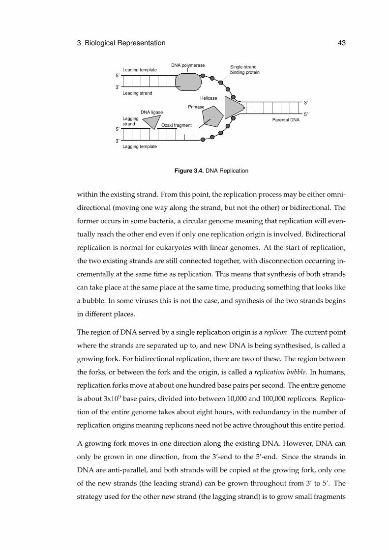
3 Biological Representation 43
3’
5’
3’
5’
5’
3’
Leading template
Leading strand
Lagging strand
Lagging template
Single-strand binding protein
Parental DNA
Helicase
PrimaseDNA ligase
DNA polymerase
Ozaki fragment
Figure 3.4. DNA Replication
within the existing strand. From this point, the replication process may be either omni-
directional (moving one way along the strand, but not the other) or bidirectional. The
former occurs in some bacteria, a circular genome meaning that replication will even-
tually reach the other end even if only one replication origin is involved. Bidirectional
replication is normal for eukaryotes with linear genomes. At the start of replication,
the two existing strands are still connected together, with disconnection occurring in-
crementally at the same time as replication. This means that synthesis of both strands
can take place at the same place at the same time, producing something that looks like
a bubble. In some viruses this is not the case, and synthesis of the two strands begins
in different places.
The region of DNA served by a single replication origin is a replicon. The current point
where the strands are separated up to, and new DNA is being synthesised, is called a
growing fork. For bidirectional replication, there are two of these. The region between
the forks, or between the fork and the origin, is called a replication bubble. In humans,
replication forks move at about one hundred base pairs per second. The entire genome
is about 3x10⁹ base pairs, divided into between 10,000 and 100,000 replicons. Replica-
tion of the entire genome takes about eight hours, with redundancy in the number of
replication origins meaning replicons need not be active throughout this entire period.
A growing fork moves in one direction along the existing DNA. However, DNA can
only be grown in one direction, from the 3’-end to the 5’-end. Since the strands in
DNA are anti-parallel, and both strands will be copied at the growing fork, only one
of the new strands (the leading strand) can be grown throughout from 3’ to 5’. The
strategy used for the other new strand (the lagging strand) is to grow small fragments
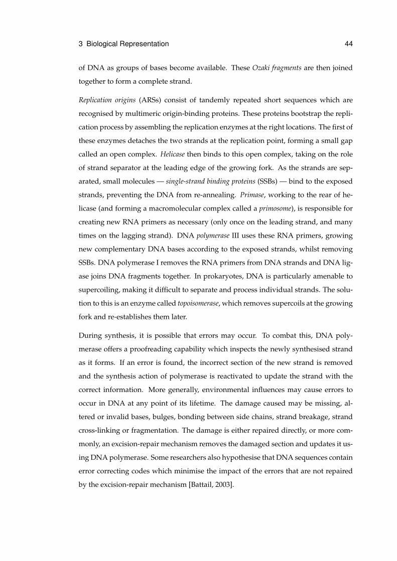
3 Biological Representation 44
of DNA as groups of bases become available. These Ozaki fragments are then joined
together to form a complete strand.
Replication origins (ARSs) consist of tandemly repeated short sequences which are
recognised by multimeric origin-binding proteins. These proteins bootstrap the repli-
cation process by assembling the replication enzymes at the right locations. The first of
these enzymes detaches the two strands at the replication point, forming a small gap
called an open complex. Helicase then binds to this open complex, taking on the role
of strand separator at the leading edge of the growing fork. As the strands are sep-
arated, small molecules — single-strand binding proteins (SSBs) — bind to the exposed
strands, preventing the DNA from re-annealing. Primase, working to the rear of he-
licase (and forming a macromolecular complex called a primosome), is responsible for
creating new RNA primers as necessary (only once on the leading strand, and many
times on the lagging strand). DNA polymerase III uses these RNA primers, growing
new complementary DNA bases according to the exposed strands, whilst removing
SSBs. DNA polymerase I removes the RNA primers from DNA strands and DNA lig-
ase joins DNA fragments together. In prokaryotes, DNA is particularly amenable to
supercoiling, making it difficult to separate and process individual strands. The solu-
tion to this is an enzyme called topoisomerase, which removes supercoils at the growing
fork and re-establishes them later.
During synthesis, it is possible that errors may occur. To combat this, DNA poly-
merase offers a proofreading capability which inspects the newly synthesised strand
as it forms. If an error is found, the incorrect section of the new strand is removed
and the synthesis action of polymerase is reactivated to update the strand with the
correct information. More generally, environmental influences may cause errors to
occur in DNA at any point of its lifetime. The damage caused may be missing, al-
tered or invalid bases, bulges, bonding between side chains, strand breakage, strand
cross-linking or fragmentation. The damage is either repaired directly, or more com-
monly, an excision-repair mechanism removes the damaged section and updates it us-
ing DNA polymerase. Some researchers also hypothesise that DNA sequences contain
error correcting codes which minimise the impact of the errors that are not repaired
by the excision-repair mechanism [Battail, 2003].
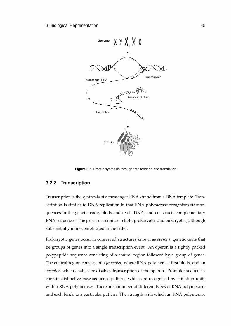
3 Biological Representation 45
Genome
Transcription
Translation
Amino acid chain
Messenger RNA
Protein
Figure 3.5. Protein synthesis through transcription and translation
3.2.2 Transcription
Transcription is the synthesis of a messenger RNA strand from a DNA template. Tran-
scription is similar to DNA replication in that RNA polymerase recognises start se-
quences in the genetic code, binds and reads DNA, and constructs complementary
RNA sequences. The process is similar in both prokaryotes and eukaryotes, although
substantially more complicated in the latter.
Prokaryotic genes occur in conserved structures known as operons, genetic units that
tie groups of genes into a single transcription event. An operon is a tightly packed
polypeptide sequence consisting of a control region followed by a group of genes.
The control region consists of a promoter, where RNA polymerase first binds, and an
operator, which enables or disables transcription of the operon. Promoter sequences
contain distinctive base-sequence patterns which are recognised by initiation units
within RNA polymerases. There are a number of different types of RNA polymerase,
and each binds to a particular pattern. The strength with which an RNA polymerase
3 Biological Representation 46
binds, and therefore the frequency at which an operon is transcribed, depends upon
how accurately a promoter implements this pattern. Hence, genes which should be
transcribed often have very accurate, or strong, promoters whereas those which are
seldom transcribed have only a passing resemblance to the ideal pattern. For most
operons, the important promoter sequences lie around ten and thirty-five bases down-
stream of the genes. The parts of the RNA polymerase that bind to these regions are
collectively called the initiation factor, or σ. The complex of subunits that continue
transcription after binding form the core polymerase. Together, the intitiation factor and
the core polymerase form a holoenzyme, a complete and functional molecule.
Operon expression is controlled by molecules (usually enzymes) called regulators
that, through binding to control locations, turn transcription on or off. Positive reg-
ulators are called activators. By binding to both promoter sequences and RNA poly-
merase, these strengthen the hold between the two, making transcription more likely.
Hence, activators make a promoter stronger. Repressors, negative regulators, do not
effect the promoter but rather bind to the operator region, blocking RNA polymerase
and preventing transcription. Operators typically consist of an inverted repeat se-
quence (a sequence followed by its repeat in reverse), each repeat forming a half-site.
Repressors are dimeric, consisting of two units, each unit binding non-covalently to
a different half-site — the bond made stable by α-helices which the repressor inserts
into major grooves of the DNA helix. A set of operons controlled by the same reg-
ulator is called a regulon. Each member of the regulon may have a different affinity
for the regulator, in the same way that different promoters have differing affinities for
a certain RNA polymerase. Certain molecules, by binding to recognition sites on the
repressor, may cause the positions of its binding α-helices to change, deactivating the
repressor. This allows repression to be enabled or disabled according to the chemical
environment. Hence, gene expression is dynamic, changing according to the products
of other genes and the current needs of the molecular system.
Not all prokaryotic genes follow the schemes outlined above. In particular, some
genes are transcribed by non-standard RNA polymerases with altered σ-factors. These
bind at many different sites, some within the normal promoter region and others in
more distant places. Also, some RNA polymerases cannot use ATP directly, requir-
ing the help of protein intermediaries. These intermediaries also bind to the DNA,
3 Biological Representation 47
often quite a distance from the operon being transcribed. Although the exception for
prokaryotes, where much gene regulation is simply metabolic response to the pres-
ence of nutrients, these more complicated systems are the norm for eukaryotes. Here,
complexity reflects the fact that genes, cells, tissues and organs all have highly-linked
actions and responses, meaning that the influences on gene expression may be far
from simple.
In eukaryotes, genes are transcribed on an individual basis rather than arranged into
operons. RNA polymerase II is responsible for the transcription of protein-encoding
genes, whereas polymerases I and III operate solely upon RNA-template genes. Eu-
rakyotic RNA polymerases do not contain an initiation factor or carry out ATP-hyd-
rolysis, relying upon DNA-binding proteins to provide these facilities. This results
in a very flexible process, with some initiation complexes consisting of many large
protein complexes. These factors bind to DNA promoters at various locations, and
through sequential interactions, guide the activity of the RNA polymerase. Eukary-
otic promoters are of several types. The strongest are TATA-boxes and initiators, similar
in structure to prokaryotic promoters. An interesting exception is the CpG (where ‘p’
denotes the phosphate bond) island, a CG repeating sequence which occurs just up-
stream of the first exon. The sequence CG is statistically under-represented in the eu-
karyotic genome, and hence stretches are easily recognised as promoters and unlikely
to be confused with other genetic information9.
Promoter sites are found anywhere between tens and tens of thousands of base pairs
away from exon sites. Promoter sites at a distance of less than two hundred base
pairs are called promoter-proximal elements, and those at a greater distance, enhancers.
Enhancers can occur upstream of exons, within introns, or even downstream of the
entire gene. Typically, multiple activator proteins will bind to a single enhancer site,
sometimes forming heterodimer complexes with members of the same class. Activa-
tors are often modular, with distinctive (even separable) DNA-binding and activation
domains. Repressors are less-well understood than activators, yet appear to have a
similar structure and capability to regulate from distant binding sites10.
9The CG dinucleotide is highly susceptible to mutation, whereby methylation causes C to mutate intoT. This explains its under-representation. A special DNA repair system protects those stretches of CpGused as promoters.
10These regulation proteins are able to bend DNA. During transcription activation, this allows distantproteins to move close together, causing large loops of DNA to appear.
3 Biological Representation 48
The purpose of transcription regulation in eukaryotes is different to prokaryotes. Pro-
karyotes are single-celled and chiefly concerned with metabolising a variety of nutri-
ents. Eukaryotes, on the other hand, are multi-cellular. Transcription regulation is the
mechanism used to make cells specialised, with the pattern of gene expression in a cell
reflecting its lineage and hence its type with respect to the surrounding tissues. Regu-
lators are inherited from the cytosol of its parent cell, and these, through transcription
regulation, decide the format of the cell’s metabolitic activity. Other regulators are
universal, passing configuration signals throughout the organism. These either act
directly, by binding to promoter regions, or indirectly, through signal transduction
pathways. For example, lipid-soluble hormones pass through cell walls and excite re-
ceptors which then release inhibitors which block the action of transcription factors.
Furthermore, lipid-insoluble hormones excite receptors on cell surfaces, which then
transmit signals through the plasma membrane to excite receptors within the cell etc
etc. In practice, far more complicated pathways exist (see section 4.2 for a full discus-
sion of signalling pathways).
Transcription in eukaryotes is made more complex by the structural organisation of
chromatin. Areas of heterochromatin, which are very compact, are inaccessible to
transcription factors. This entails that transcription cannot take place during cell-
division. Furthermore, certain sections of chromatin remain condensed during inter-
phase. These areas are not transcribed — even though theoretically-active genes exist
within them. Some of these areas have become unused over evolutionary time, mak-
ing it more efficient for them to remain compressed. Other areas are only found com-
pressed in certain cells. This form of regulation is equivalent to regulator molecules in
the cytosol, making the cell specialised. Human females inherit two X-chromosomes
from their parents. Early on in development, one of these chromosomes becomes,
and remains, condensed. Hence, only one of the human X-chromosomes, decided
randomly, is transcribed in a given human.
Finally, mitochondria and chloroplasts have gene transcription systems similar to pro-
karyotes. Both these organelles have small genomes encoding a small number of pro-
teins. Mitochondria, in particular, have very simple transcription systems — with mi-
tochondrial RNA polymerase being the simplest protein that can carry out all stages
of transcription.
3 Biological Representation 49
3.2.3 Cell Division
For prokaryotes, cell-division and reproduction11 are typically the same thing. The
circular DNA within the cell becomes attached to the cell membrane. The DNA repli-
cates, separates, and the new strand becomes attached to the plasma membrane at a
different, but nearby, point. The membrane between the two attachment points and
the membrane on the opposite side of the cell then move together. When they join, the
cell separates into two daughter cells — each with its own DNA and a fifty percent
share of the original cytosol.
The cell cycle for eukaryotes is somewhat more complicated and can be expressed by
two different processes, mitosis and meiosis. Mitosis is normal cell division, account-
ing for regeneration and growth and producing daughter cells that are genetically
identical. Meiosis is the production of germ cells (eggs and sperm) to meet reproduc-
tive needs, generating daughter cells that are genetically different.
Mitosis
The mitotic cell cycle consists of four phases, illustrated in figure 3.6. At the beginning
is a gap of inactivity, during which the cell goes about its normal metabolic functions.
At some point in time, depending upon the type of cell and how frequently it should
divide, the cell enters the synthesis phase — during which nuclear DNA is replicated
to produce two identical sets. Following from this is another, shorter, gap of inactivity,
concluded by the mitotic phase. The mitotic phase, in turn, is carried out in four stages.
In eukaryotes, it is normal for nuclear DNA to be split into a number of units, each con-
tained within its own macromolecular complex. This complex is called a chromosome
and consists of a single molecule of DNA bonded to various proteins and structural
members. In sexual species, there are two sets of chromosomes — the maternal and
the paternal — inherited, respectively, from the organism’s mother and father. After
the synthesis stage of mitosis — where chromosomes are duplicated — each chromo-
some remains attached to its duplicate, forming a structure called a sister chromatid.
Since this is the only time when chromosomes become easily visible in a microscope,
11Sexually reproducing bacteria do so by horizontal gene transfer, whereby a section of DNA from onebacteria invades the DNA of another. This can occur whenever the bacteria are in proximity.
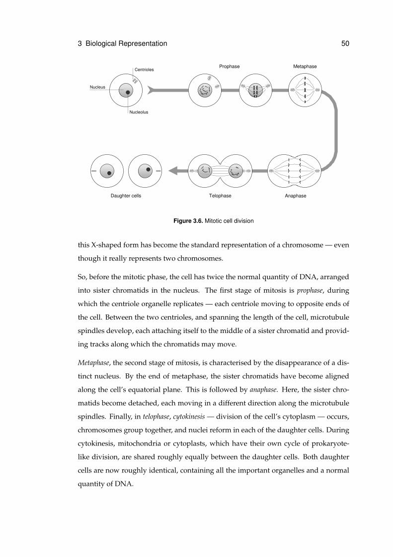
3 Biological Representation 50
Prophase Metaphase
AnaphaseTelophase
Nucleolus
Centrioles
Nucleus
Daughter�cells
Figure 3.6. Mitotic cell division
this X-shaped form has become the standard representation of a chromosome — even
though it really represents two chromosomes.
So, before the mitotic phase, the cell has twice the normal quantity of DNA, arranged
into sister chromatids in the nucleus. The first stage of mitosis is prophase, during
which the centriole organelle replicates — each centriole moving to opposite ends of
the cell. Between the two centrioles, and spanning the length of the cell, microtubule
spindles develop, each attaching itself to the middle of a sister chromatid and provid-
ing tracks along which the chromatids may move.
Metaphase, the second stage of mitosis, is characterised by the disappearance of a dis-
tinct nucleus. By the end of metaphase, the sister chromatids have become aligned
along the cell’s equatorial plane. This is followed by anaphase. Here, the sister chro-
matids become detached, each moving in a different direction along the microtubule
spindles. Finally, in telophase, cytokinesis — division of the cell’s cytoplasm — occurs,
chromosomes group together, and nuclei reform in each of the daughter cells. During
cytokinesis, mitochondria or cytoplasts, which have their own cycle of prokaryote-
like division, are shared roughly equally between the daughter cells. Both daughter
cells are now roughly identical, containing all the important organelles and a normal
quantity of DNA.
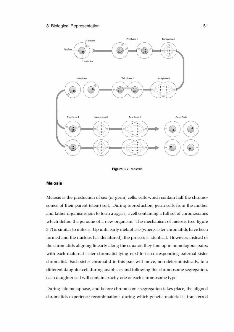
3 Biological Representation 51
Prophase�I Metaphase�I
Anaphase�ITelophase�I
Nucleolus
Centrioles
Nucleus
Interphase
Prophase�II Metaphase�II Anaphase�II Germ�Cells
Figure 3.7. Meiosis
Meiosis
Meiosis is the production of sex (or germ) cells; cells which contain half the chromo-
somes of their parent (stem) cell. During reproduction, germ cells from the mother
and father organisms join to form a zygote, a cell containing a full set of chromosomes
which define the genome of a new organism. The mechanism of meiosis (see figure
3.7) is similar to mitosis. Up until early metaphase (where sister chromatids have been
formed and the nucleus has denatured), the process is identical. However, instead of
the chromatids aligning linearly along the equator, they line up in homologous pairs;
with each maternal sister chromatid lying next to its corresponding paternal sister
chromatid. Each sister chromatid in this pair will move, non-deterministically, to a
different daughter cell during anaphase; and following this chromosome segregation,
each daughter cell will contain exactly one of each chromosome type.
During late metaphase, and before chromosome segregation takes place, the aligned
chromatids experience recombination: during which genetic material is transferred
3 Biological Representation 52
between the chromatids. Recombination involves a process called crossover: the ex-
changing of sections of DNA between the chromosomes; and although not explicitly
transferring genes, this is the most likely outcome. The mechanism of crossover is
explained in the following section. Following recombination, within anaphase and
telophase, each homologue of a sister chromatid pair moves towards a different end
of the cell and cytokinesis occurs. Unlike in mitosis, the sister chromatids do not split
into separate chromosomes. The result is two daughter cells, each containing the nor-
mal amount of DNA, arranged into sister chromatids. Since the aim is to have half the
normal amount of DNA, a second phase of cell division occurs with the chromatids
detaching and segregating as in mitosis: finally resulting in four germ cells being pro-
duced from a single stem cell, each of which is genetically different to all the others.
Recombination
Recombination occurs at the end of metaphase when pairs of homologous sister chro-
matids have become aligned at the cellular equator. This alignment is called synapsis.
Crossover is the swapping of genetic material between chromatids bought into close
contact by synapsis. A number of points are randomly selected along the length of the
two chromatids and sections of the DNA occurring between every other pair of points
are swapped. Compared to the length of the chromatids, these crossover points are in-
numerous and are most likely to occur within regions of non-coding DNA. Therefore,
the effect is that genes, or groups of genes, move between pairs of chromosomes. Most
of the time, the integrity of genes are unaffected. Sometimes a crossover point will oc-
cur within a gene and, most likely, this will result in a novel gene formed from parts
of the paternal and maternal versions. However, since chromosomes do not always
align perfectly, there is some chance of this new gene not working correctly.
The Holliday model was the first to offer a satisfactory explanation of the mechanism
behind crossover. At synapsis, both chromosomal duplexes align. Under the control
of enzymes, a nick is made in a single DNA strand in one of the chromosomes. At this
point, a small section of the nicked strand becomes detached from its complementary
strand and invades the other chromosome, which is nicked at the same point, ligat-
ing to the corresponding strand. The same effect happens with the displaced strand
from the other chromosome, forming a crossed-strand Holliday structure. This crossed
3 Biological Representation 53
section linking the chromosomes is mobile, able to move in either direction along the
DNA complex. Under enzymatic influence, the crossed section moves a random dis-
tance — a process called branch migration — further detaching sections of single-strand
DNA and carrying them over to the other chromosome. Rotation around the crossed
section, the crossover point, results in an isomeric Holliday structure, a cross-shaped
formation characteristic of recombination. Further nicks and resealings, driven by en-
zymatic action, produce one of two different end structures — recombinative or non-
recombinative. Both of these contain heteroduplexes, sections of non-complementary
duplex DNA. These will either be repaired by the DNA excision-repair mechanism, or
remain heteroduplex until the next cell division. At this point, each daughter chromo-
some will gain a different section of DNA corresponding to the two halves of the het-
eroduplex. In recombinant DNA, sections of duplex DNA have transferred between
chromosomes. Heteroduplexes occur around the joining point. In non-recombinative
DNA, only small sections of single-strand DNA have been transferred between chro-
mosomes. The excision-repair mechanism can update from either the existing strand,
replacing the transferred single-strand, or from the invading strand. If crossover oc-
curs within a gene, this latter action will cause gene conversion, the updating of an
exon with new code.
4 Biochemical Pathways
Having introduced the key components of biological systems — cells, genes and pro-
teins — these elements can now be bought together to describe higher-level struc-
tures which form the basis of control and function within biological organisms. These
structures, called biochemical pathways, form networks of computation and commu-
nication which permeate organisms, bringing about order through the control and
co-ordination of the activity of local systems.
There are three categories of biochemical pathway (see figure 4.1). Metabolic net-
works exist within cells, emerging from interactions between locally-transcribed pro-
teins. Signalling networks comprise cellular responses to inter-cellular signals. Gene ex-
pression networks describe regulatory interactions between genes and gene-products.
Marijuan [1995] describes these activities, respectively, as self-organisation, self-reshaping
and self-modification. Self-organisation reflects how a distributed system of indepen-
dent components can carry out a unified process. Self-reshaping is the ability of
an existing system to carry out multiple processes to satisfy varying needs. Self-
modification is the ability of a system to change its constitution in order to solve un-
foreseen problems. Interactions between the three classes of pathway unifies these
processes and bring out the emergent behaviour of the whole organism.
4.1 Metabolic Networks
The previous chapter introduced the structure and function of individual proteins and
enzymes, their capacity to interact — through sharing of products and substrates —
and their mechanisms of regulation: activation, inhibition and allosterism. This sec-
54
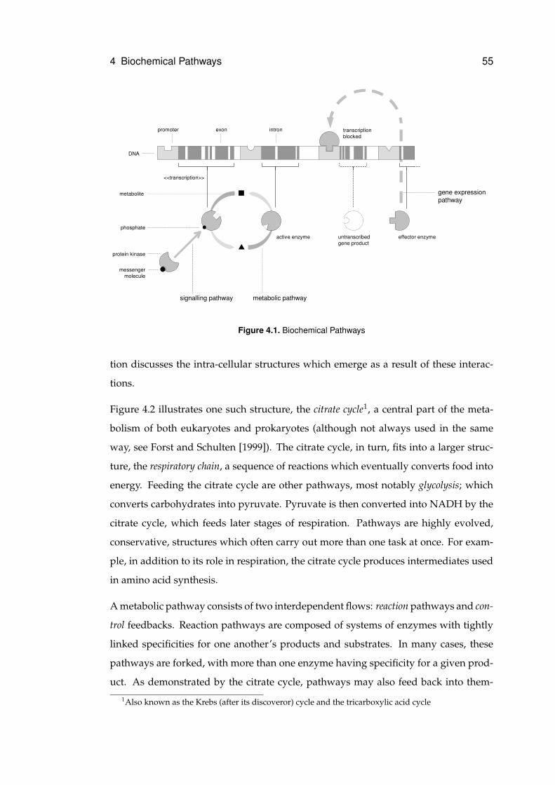
4 Biochemical Pathways 55
gene�expression�pathway
metabolic�pathwaysignalling�pathway
effector�enzymeuntranscribed�gene�product
phosphate
metabolite
active�enzyme
promoter exon intron
DNA
protein�kinase
messenger�molecule
transcription�blocked
<<transcription>>
Figure 4.1. Biochemical Pathways
tion discusses the intra-cellular structures which emerge as a result of these interac-
tions.
Figure 4.2 illustrates one such structure, the citrate cycle1, a central part of the meta-
bolism of both eukaryotes and prokaryotes (although not always used in the same
way, see Forst and Schulten [1999]). The citrate cycle, in turn, fits into a larger struc-
ture, the respiratory chain, a sequence of reactions which eventually converts food into
energy. Feeding the citrate cycle are other pathways, most notably glycolysis; which
converts carbohydrates into pyruvate. Pyruvate is then converted into NADH by the
citrate cycle, which feeds later stages of respiration. Pathways are highly evolved,
conservative, structures which often carry out more than one task at once. For exam-
ple, in addition to its role in respiration, the citrate cycle produces intermediates used
in amino acid synthesis.
A metabolic pathway consists of two interdependent flows: reaction pathways and con-
trol feedbacks. Reaction pathways are composed of systems of enzymes with tightly
linked specificities for one another’s products and substrates. In many cases, these
pathways are forked, with more than one enzyme having specificity for a given prod-
uct. As demonstrated by the citrate cycle, pathways may also feed back into them-
1Also known as the Krebs (after its discoveror) cycle and the tricarboxylic acid cycle
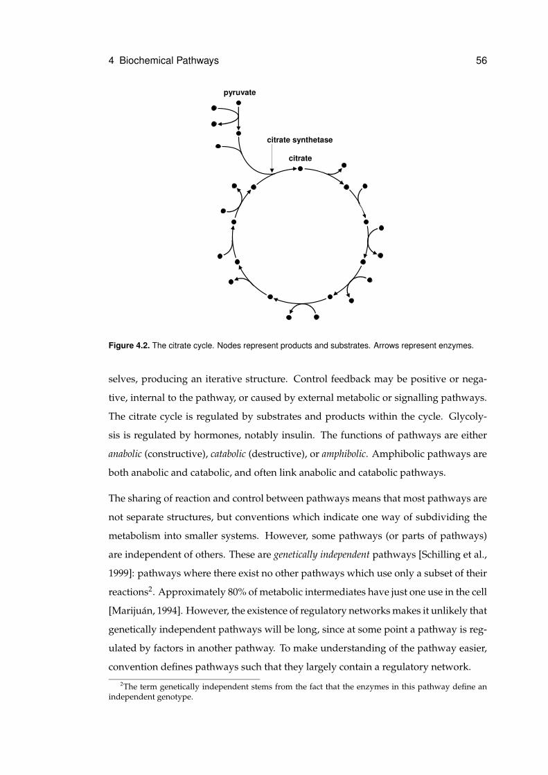
4 Biochemical Pathways 56
citrate
pyruvate
citrate synthetase
Figure 4.2. The citrate cycle. Nodes represent products and substrates. Arrows represent enzymes.
selves, producing an iterative structure. Control feedback may be positive or nega-
tive, internal to the pathway, or caused by external metabolic or signalling pathways.
The citrate cycle is regulated by substrates and products within the cycle. Glycoly-
sis is regulated by hormones, notably insulin. The functions of pathways are either
anabolic (constructive), catabolic (destructive), or amphibolic. Amphibolic pathways are
both anabolic and catabolic, and often link anabolic and catabolic pathways.
The sharing of reaction and control between pathways means that most pathways are
not separate structures, but conventions which indicate one way of subdividing the
metabolism into smaller systems. However, some pathways (or parts of pathways)
are independent of others. These are genetically independent pathways [Schilling et al.,
1999]: pathways where there exist no other pathways which use only a subset of their
reactions2. Approximately 80% of metabolic intermediates have just one use in the cell
[Marijuan, 1994]. However, the existence of regulatory networks makes it unlikely that
genetically independent pathways will be long, since at some point a pathway is reg-
ulated by factors in another pathway. To make understanding of the pathway easier,
convention defines pathways such that they largely contain a regulatory network.
2The term genetically independent stems from the fact that the enzymes in this pathway define anindependent genotype.
4 Biochemical Pathways 57
Even though many key reaction pathways have been identified and charted, the meta-
bolism is still not completely understood. As a result, known pathways tend to reflect
incomplete knowledge, describing a subset of the operation of actual metabolisms.
Factors such as re-use of reactions, multiple equivalent paths through the network,
and variety between cell types and between individuals (since our genomes are not
identical) add to the difficulty of understanding. Fortunately, with the genomes of a
number of organisms now completely sequenced, the data required to fuel this under-
standing is becoming available. The difficult task now is in interpreting this data, a
task undertaken by traditional mathematical techniques [Heinrich and Schuster, 1998],
modelling [Reddy et al., 1993, 1996], and bioinformatics [Schilling et al., 1999]. A bet-
ter understanding of the metabolism would have many uses, including those in bio-
process engineering (creation of novel metabolic pathways for use in chemical plants)
and health-related (finding alternative paths through defective networks, design of
drugs which intervene in the metabolism) areas [Karp and Mavrovouniotis, 1994].
Current understanding is expressed through charts and diagrams [Michal, 1999] (for
which representation is a key concern [Michal, 1998, Karp and Paley, 1994]) and public
databases [Karp, 1999, European Bioinformatics Institute, 2000].
Finally, understanding of the metabolism can be aided by an understanding of how it
evolved. This topic has been approached from a number of areas, including biochem-
istry [Lyubarev and Kurganov, 1997, Wachtershauser, 1990], biophysics [Igamberdiev,
1999] and molecular evolution [Page and Holmes, 1998, Forst and Schulten, 1999]. The
molecular evolution approach uses the current form of genomes to infer properties of
earlier forms. For example, in many cases enzymes proximal in a pathway are also
proximal in the genome, since they must have had a high degree of genetic linkage in
order to have survived recombination events during evolution.
4.2 Signalling Networks
Signalling between cells in an organism is a fairly well understood process. Cells pro-
duce signal proteins which, after being released through the cell’s plasma membrane,
spread throughout the organism via bodily fluids. Receptors on the surface of other
cells then detect this signal and relay it to the appropriate components within the cell.
4 Biochemical Pathways 58
How this intra-cellular communication happens, by comparison, is only now begin-
ning to be understood by molecular biologists.
In fact, research shows this process to be surprisingly complex — not simply a case
of a receptor generating the right signal and transmitting this into the cytoplasm —
but rather an extended series of events involving many different agents. Key amongst
these agents are protein kinases and phosphotases, enzymes which modify the activity of
other enzymes. Other players include secondary messenger molecules, protein adapters
— which connect other proteins together — and scaffold proteins — which co-ordinate
the activities of other molecules.
Under the classic model [Sutherland, 1972, Fisher et al., 1999], occupation of a recep-
tor by an external signal molecule causes the activation of an internally-bound effector
enzyme. This effector then generates secondary messenger molecules which spread
the signal throughout the cell and activate target proteins. These signal sensitive pro-
tein kinases or phosphotases then, either directly or indirectly via the (in)activation of
other protein kinases or phosphotases, modify proteins within the metabolic or gene
expression networks of the cell. This brings about a change in cellular activity. Of par-
ticular note is the degree of amplification involved in the system: one primary signal
molecule causes many secondary signal molecules which then activate a hierarchy of
modifier proteins.
More recent research (summarised in [Scott and Pawson, 2000]) refines this under-
standing. Many receptors are in the family receptor tyrosine kinase. These enzymatic
proteins work in pairs. When a pair of receptors bind signal hormones, their cytoplas-
mic tails (which protrude below the plasma membrane) bind phosphate molecules to
one another’s tyrosine amino acids. These altered residues then become bound, either
directly, or indirectly through adapters, to signalling enzymes — activating the sig-
nalling enzymes, causing them to generate secondary messenger molecules (see figure
4.3). The key differences in this new interpretation are that: (i) signalling proteins typ-
ically consist of multiple domains; and (ii) these proteins are spatially co-ordinated.
In more complicated signalling systems, scaffold proteins, which consist of multiple
linker domains, provide this co-ordination. Indeed, they are particularly prevalent in
hierarchical protein kinase/phosphotase systems. This is necessary because these en-
zymes often have broad specificity, meaning that if not co-ordinated, they can modify
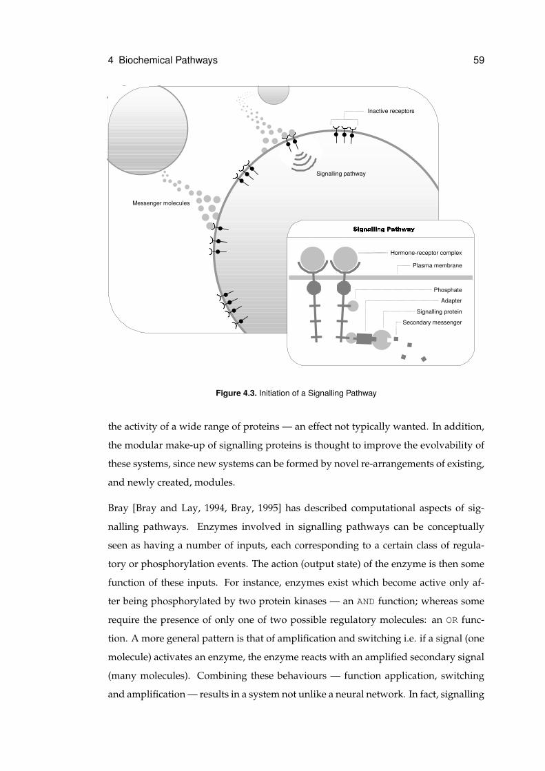
4 Biochemical Pathways 59
Inactive�receptors
Messenger�molecules
Signalling�pathway
8�9 :�;=<?> > 9 ;=:A@B<BCEDGF+<IH
Hormone-receptor�complex
Plasma�membrane
Phosphate
Adapter
Signalling�protein
Secondary�messenger
Figure 4.3. Initiation of a Signalling Pathway
the activity of a wide range of proteins — an effect not typically wanted. In addition,
the modular make-up of signalling proteins is thought to improve the evolvability of
these systems, since new systems can be formed by novel re-arrangements of existing,
and newly created, modules.
Bray [Bray and Lay, 1994, Bray, 1995] has described computational aspects of sig-
nalling pathways. Enzymes involved in signalling pathways can be conceptually
seen as having a number of inputs, each corresponding to a certain class of regula-
tory or phosphorylation events. The action (output state) of the enzyme is then some
function of these inputs. For instance, enzymes exist which become active only af-
ter being phosphorylated by two protein kinases — an AND function; whereas some
require the presence of only one of two possible regulatory molecules: an OR func-
tion. A more general pattern is that of amplification and switching i.e. if a signal (one
molecule) activates an enzyme, the enzyme reacts with an amplified secondary signal
(many molecules). Combining these behaviours — function application, switching
and amplification — results in a system not unlike a neural network. In fact, signalling
4 Biochemical Pathways 60
enzymes are more like McCulloch-Pitts neurons (perceptrons) than are real neurons.
Taking this idea further, Bray has experimented with abstract models of these ‘protein
circuits’, using simulated evolution (optimising reaction rates and binding constants)
as a training system.
The switching behaviour of an enzyme depends upon a number of kinetic properties:
properties which affect the speed and crispness of responses. However, the quantum
mechanical behaviour of enzymatic reactions means that they do not always behave
as ideal Boolean switches, but display varying degrees of fuzzy response. Bray sug-
gests that this behaviour is caused by asymmetries and synergisms between inputs;
and results in enzymes behaving like fuzzy logic elements, which may be more com-
putationally powerful than Boolean logic units. Fisher et al. [1999], too, discuss the
fuzzy properties of signalling enzymes, particularly protein kinases, comparing their
behaviour to fuzzy classifier systems. Moreover, they describes the ‘signalling ecol-
ogy’ as a “vast parallel distributed processing network of adaptable agents”, confer-
ring such cognitive properties as pattern recognition, handling fuzzy data, memory
capacity and context-sensitivity to these agents.
4.3 Gene Expression
A cell’s type is defined by the subset of genes which are typically expressed (tran-
scribed) within the cell. Recall from section 3.2.2 that transcription of a particular
gene depends upon the correct formation and activity of a transcription complex, a
process which can be blocked by the binding of certain inhibitors to regulation sites
associated with the gene. Inhibitors are proteins and therefore must be encoded by
other genes. Each of these regulating genes, in turn, may be regulated by inhibitors
encoded by other genes. Typically, a single regulating gene may regulate a small num-
ber of other genes, each of which may then, in turn, regulate a small number of other
genes. By transitivity, a single gene may indirectly affect the regulation of a large
number of other genes. A gene may also, either directly or indirectly, regulate its own
transcription. This complex system of regulatory interactions is known variously as a
gene expression network, a genomic regulatory network, or more concisely, a genetic
network.
4 Biochemical Pathways 61
Genetic networks are not easy to understand and, like all discrete dynamical net-
works, are difficult to analyse using partial differential equations and other techniques
from continuous mathematics. Hence, they are typically modelled with automata and
analysed by simulation, a trend captured by Stuart Kauffman in the form of random
boolean networks (RBN’s) [Kauffman, 1969, Somogyi and Sniegoski, 1996]. These de-
scribe regulatory networks as a mapping from state t to state t + 1, employing di-
rectional links, binary on/off states, parallel updates and combinatorial logic on in-
puts. Whilst an idealised representation, these abstract networks still demonstrate
behaviour similar to real networks. Interestingly, when simulated, the networks in-
dicate the existence of attractors, which pull the network towards a small set of final
states starting from a large number of initial states. In [Somogyi and Sniegoski, 1996,
Wuensche, 1998], this behaviour is compared to specialisation in cells with an attrac-
tor comparable to a single cell type and paths between attractors equivalent to path-
ways of differentiation. Following from this, a cell type can be expressed as a set of
closely related gene expression patterns, centered around a basin of attraction. It is
also conjectured that the strength of this attractor must represent a balance between
a cell’s adaptiveness and a need not to cross to neighbouring states (which could, for
instance, correspond to cancer cells).
As well as being dynamic and self-adaptive in their own right, networks of genetic
expression are also directly subject to evolution. In [Shimeld, 1999], this evolution is
discussed in terms of gene duplication events. In [Bornholdt and Sneppen, 1998, Born-
holdt and Rohlf, 2000] artificial evolution is used to evolve connectivity in Boolean
(and other dynamical) networks. In [Bignone et al., 1997], evolution of genetic net-
works is considered from a mathematical perspective.
Chiva and Tarroux [1995], too, have applied simulated evolution in order to gain
a greater understanding of how biochemical networks develop. Their system in-
cludes both transcriptional (gene regulation) and post-translational (protein interac-
tions) components, reflecting the coupling between genes and gene-products — and
the influence of both in the gene regulation process. These ‘protein regulation net-
works’ are deterministic, recurrent and synchronous. The activation state (concentra-
tion) of a unit (protein) is a weighted sum of activations of other units. The weights
are defined in a genome, where a gene represents each protein. Gene expression is
4 Biochemical Pathways 62
defined by two sets: the set of states where this protein may be regulated by others,
and the set of states where this protein may regulate others. The intent is that the
model should mimic protein folding. The algorithm used is a genetic algorithm with
uniform crossover, a degree of steady-state and a set (no duplicates) as the population
structure. The last point is meant to reduce genetic drift. Gene duplication and new
gene events take place population-wide at fixed intervals (keeping all solutions the
same length). The system is intended to emulate differentiation, triggered by external
stimuli. Hence, the fitness function rewards solutions which change state when given
pertinent stimuli and punishes those which differentiate with false or vacant signals.
Communication signals are implemented with ‘clamped’ units, whose concentration
(activation) is externally dictated.
A key observation is that a gradual increase in solution size from N0 to N1 produced
markedly superior results than fixing solution size at either N0 or N1. This suggests
that gene networks evolve best by building upon existing, smaller, networks — an
observation that explains why yeast and humans share similar pathways; the human
pathways including the yeast pathways as subsets of their possible reactions. The
explanation behind this phenomenon is that evolution in smaller networks is much
more likely to find the local optimum, whereas evolution in a larger network is harder.
For a larger network to evolve, it must go via stable intermediate states — which are
provided explicitly by smaller networks.
Another observation is the development of ‘command units’, those for which fan-out
is of much higher intensity than fan-in — amplification — and for whom input signals
are heterogenous, whereas output signals are homogenous. This causes the formation
of hierarchies, similar to those found in biological signalling pathways. Finally, the
genome encoding used implicitly made the network fully-connected (although some
of these connections may be ignored by a given unit). The authors speculate that
sparsely-connected networks, corresponding to biological systems, might provide a
better opportunity to develop clusters of specialised function within the network.
5 Biological Evolvability
Many definitions exist for the term ‘evolvability’. The most general of these is ”the
capacity to evolve” [e.g. Smith et al., 2003] i.e. the capacity for some entity or group
of entities to undergo change, or as Suzuki [2003] puts it, ”the possibility (potential
ability) of evolving a variety of genotypes or phenotypes”. Most, however, agree on a
more limited definition of evolvability: summarised by Nehaniv [2003] as ”the ability
to reach ‘good’ solutions via evolution”, and implicitly appealing to a requirement for
direction within evolution. Likewise, Altenberg [1994] offers ”the ability of a popu-
lation to produce variants fitter than any yet existing”; Wagner and Altenberg [1996]:
”the genome’s ability to produce adaptive variants when acted on by the genetic sys-
tem”; and Kirschner and Gerhart [1998]: ”the capacity to generate heritable selectable
phenotypic variation”. A key issue addressed by these definitions is access to adapta-
tion: the degree to which the evolving system is able to gain adaptive traits (termed
‘accessibility’ in Volkert [2003]) and the amount of evolution required to transform the
existing system into a system which possesses these traits. Also important for evolv-
ability, though implied rather than stated explicitly in these definitions, is the mainte-
nance of existing traits: without which the gaining of new traits is largely academic.
To use Kirschner and Gerhart’s own words, evolvability (in a biological context) re-
quires a capacity ”(i) to reduce the potential lethality of mutations and (ii) to reduce
the number of mutations needed to produce phenotypically novel traits” [Kirschner
and Gerhart, 1998].
In part due to its unfortunate association with ideas of group selection, the study of
evolvability is still in its relative infancy. Nevertheless, as understanding of biology,
complex systems and, more recently, evolutionary computation has increased; it has
become apparent that considerable insight can be made into evolvability phenom-
63
5 Biological Evolvability 64
ena. Research into evolvability follows three broad themes: (i) the characteristics of
evolvable systems and the requirements for a system to exhibit evolvability; (ii) ac-
tual sources of evolvability within biological and non-biological systems; and (iii) the
evolution of evolvability.
Some of the most significant insights into evolvability have been made by Michael
Conrad [1979, 1985, 1990]. In particular, he speculates that evolvable systems are
a very unique kind of system that reflects a balance between the need for pheno-
typic stability on the one hand and the pressure towards genetic exploration on the
other. Following from studies of complex systems, it is known that the functioning
of randomly-connected systems becomes more unstable as complexity increases yet
more sensitive to (e.g. genetic) change as complexity decreases. According to Conrad
[1990], these competing pressures can only be satisfied in systems that display com-
partmentalisation, component redundancy, and multiple weak interactions.
5.1 Compartmentalisation
Of these requirements, compartmentalisation is perhaps easiest to understand. A
compartment is a group of components whose interactions are mostly internal to the
group. Consequently, a change (e.g. due to genetic variation) within one of the group’s
components is most likely to have its effect limited to other members of the group
rather than percolating to the entire system. Likewise, multiple changes to the system
are likely to affect separate sub-systems rather than have a compound (and probably
lethal) effect upon a single sub-system. In Kirschner and Gerhart [1998], the authors
describe compartmentalisation as a significant source of de-constraint within biolog-
ical organisation. Constraints upon evolutionary change occur where one part of a
system in unable to change because of the un-welcome effects a change would have
upon other parts of the system to which it has strong linkage. An example of con-
straint is where a gene codes for an enzyme which carries out different roles within
more than one different pathway or the same pathway carrying out a different role
within a different type of cell; and where a change to the gene would improve its
function within one context but lead to a lethal change within the other. If, however,
the enzymes within both contexts were coded by separate genes, then both enzymes
5 Biological Evolvability 65
could vary — and be selected for — independently. Following this logic, it would
make evolutionary sense to have genetic independence between both pathways.
However, in Hansen [2003b] the author argues that modularisation is not always the
best solution for evolvability. In actual biological systems, there exists a substantial
level of pleiotropy between characters: with one gene having an influence (via use of
the same protein) upon the function of more than one tissue, organ or trait. Hansen
suggests that this is due to increased variational potential out-weighing the interfer-
ence caused by pleiotropy. In particular, it would seem that pleiotropy should be en-
couraged in the early stages of adaptation, with an evolving sub-system making use
of functional building blocks used elsewhere within the organism. Depending upon
the selective pressure placed upon the two sub-systems, their sensitivity to change,
and the role of the shared function, it might then make continued sense for the shared
function to co-adapt within both systems via this pleiotropic link. Indeed, Hansen
suggests that in some cases the evolution of modularity may not be a necessary con-
dition for the evolution of evolvability.
One process in which compartmentalisation appears to play a crucial role is during the
embryonic development of multi-cellular organisms [Kirschner and Gerhart, 1998].
Development is characterised by the differentiation of the organism into increasingly
more specialised compartments. The initial segmentation of the embryo is dependent
upon concentration biases in the fertilised egg. However, as development proceeds,
separate compartments rapidly become independent of the activities — and therefore
of the errors — occurring in other compartments. Hence, a failure caused by genetic
change (or otherwise) in one compartment will not impede upon the development
of the entire system. Likewise, evolution can carry out morphological exploration
within one compartment without affecting other compartments: another example of
de-constraint.
Compartmentalisation also appears within the spatial arrangement of genes within a
genome. This phenomenon, called epistatic clustering, occurs in both prokaryotes and
eukaryotes. In prokaryotes, it is particularly apparent in the form of operons: where a
group of genes with tightly-linked products are located proximal in the genome and
are transcribed within a single transcription event. Functionally, this is advantageous
for prokaryotes because they save time and energy when expressing new pathways
5 Biological Evolvability 66
in response to changes in the environment. However, it also aids evolvability by im-
proving the efficacy of horizontal gene transfer since, due to their proximal locations
in the genome, it is likely that the genes in an operon would be transferred to other
prokaryotes as a single unit. The other prokaryote would in effect receive an entire
metabolic pathway, which is far more likely to improve its fitness than a group of un-
related genes [Poole et al., 2003]. Eukaryotes, by comparison, transfer genes during
sexual recombination. After crossover, a pathway is more likely to be preserved if the
genes which code for it are located close together within a chromosome. Evolvability
might therefore be improved in a genome which expresses modularity in the form of
epistatic clustering [Pepper, 2003].
5.2 Redundancy
Redundancy appears in many forms in biological systems. This section introduces
functional redundancy, structural redundancy, and weak linkage.
5.2.1 Functional redundancy
Examples of functional redundancy in biology include: at the genomic level, gene
families, pseudo-genes and polyploidy; and at the phenotypic level, allozymes (func-
tionally equivalent enzymes) and homogenous tissues. In a sense, functional redun-
dancy is another form of compartmentalisation where functionally similar, or equiva-
lent, components conceptually form groups that limit the affect of perturbations from
other kinds of component [Conrad, 1990]. This buffering occurs in response to both
genetic change: where redundant copies help maintain the previous role of the com-
ponent that has been changed; and phenotypic perturbation: by allowing multiple
steady states in the space of phenotypic behaviour. Consequently, functional redun-
dancy provides a means of overcoming the opposing requirements for phenotypic
stability and the increased complexity (more components) needed to support genetic
change.
Functional redundancy underlies Ohno’s theory of ‘evolution by gene duplication’
[Ohno, 1970]. This theory proposes that the majority of molecular evolution has oc-
5 Biological Evolvability 67
curred through a process of gene duplication and divergence: whereby genes recur-
sively duplicate (possibly through misaligned crossover) and evolve separately into
genes that encode proteins with increasingly more specialised functions. (This pro-
cess may also be involved in the evolution of modularity — see Wagner and Altenberg
[1996].)
5.2.2 Structural redundancy
Structural redundancy occurs where biological components such as proteins, chromo-
somes, and pathways have higher complexity than is required to fulfill their pheno-
typic task. Structural redundancy improves evolvability by acting as a genetic buffer-
ing mechanism which limits or gradualises the effect of genetic change. An example
is non-coding DNA, which effectively segregates genes, making it more likely that
crossover junctions will form between, rather than within, genes: and therefore lim-
iting the disruptiveness of recombination. Another example (see section 5.3) is the
mutation buffering provided by redundant amino acids during the evolution of pro-
tein structures. Structural redundancy can also enable the formation of new evolu-
tionary mechanisms. A good example is transposons, which make use of structural
redundancy within the genome and may play a role in producing mutational hot-spots
(where genetic change occurs faster than in other regions of the genome) in addition
to their roles (described earlier) in gene duplication and gene formation.
5.2.3 Weak Linkage
Weak interactions are another form of redundancy, but one that occurs at the inter-
connection level. A weak interaction has a small informational effect: such as the
bond made by an individual amino acid at an enzyme’s binding site; whereas a strong
interaction has a large informational effect: such as the binding of a substrate at a
binding site. In the case of weak interactions, the net effect is one of integration — the
summing of the effect of multiple weak interactions from many different sources. Re-
moving or adding a single interaction will have little effect upon this sum, and hence
the effect it produces. For strong interactions, by comparison, each interaction is capa-
ble of having a decisive effect: for example, the inputs to a logical AND function are
5 Biological Evolvability 68
strong signals since each can individually determine the output of the function. Ac-
cording to Conrad [1990], redundancy through multiple weak interactions is the best
way of compromising genetic instability and phenotypic stability within a system,
since it allows a system to have many components and interactions (and therefore a
high degree of genetic control) whilst limiting the impact of any particular component
or interaction (and therefore the effect of a phenotypic change).
A small genetic change to a weak interaction will typically lead to a small phenotypic
change. This means that a system with weak interactions is highly controllable at
the genetic level, and suggests why weak interactions are a key component of many
evolvable structures seen in biology. The benefit of weak interactions can also be seen
in results by Volkert and Conrad [1998] and Volkert [2003] in the context of enhanc-
ing evolvability in a non-biological system. In this work, the authors studied the be-
haviour of random and evolved dynamic network models (non-uniform cellular au-
tomata) with and without weak interactions; and found that weak interactions could
improve the exploratory scope (access to behaviours), the performance of evolved net-
works, and the stability of evolved networks when exposed to random genetic muta-
tion.
Weak interactions occur extensively in regulatory pathways. Regulatory pathways, in
turn, are thought to have been of considerable importance to the evolution of complex
multi-cellular organisms [Kirschner and Gerhart, 1998]. Examples of multiple weak
interactions are the calcium ions whose concentration controls the secretion of neu-
rotransmitters in the brain; and the interactions between the binding site, enzymes,
enhancers, and control signals that lead to the formation of a transcription complex
in eukaryotes. In each of these cases it is the net effect of all of the interactions that
controls the activation level. Because of this, the strength of activation can be varied
gradually through the addition and removal of components and interactions, and can
respond flexibly to new sources of regulation.
5.3 Evolution through Redundancy
The effect of redundancy is to increase the tunability of evolution such that most mu-
tations lead to small or neutral changes to an organism’s fitness. Proteins, for exam-
5 Biological Evolvability 69
ple, exhibit all three forms of redundancy discussed above. Functional redundancy
results from the presence of gene families and polyploidy and reduces the impact of
deleterious variants by offering functional alternatives. Structural redundancy results
from the presence of extra amino acids and allows a protein’s shape (and therefore
its activity) to be varied more gradually than a protein with no structural redundancy.
Weak linkage occurs during protein folding where weak interactions such as hydrogen
bonding, hydrophilic interaction and Van der Walls interactions produce the protein’s
functional shape: and allows small changes in the protein’s shape and chemistry by
adding and removing bonds. The shape of the protein, in effect, can evolve along
either of these redundancy axes through a process of gradual change which Conrad
[1985] calls mutation buffering to reflect the fact that a protein, or other structure, can
experience a number of mutations with little or no change to its functionality. Evolu-
tion through redundancy, in this respect, is a clear example of how neutral evolution
can lead to adaptation.
Conrad [1979, 1990] has attempted to explain the role of redundancy in evolution
by appealing to the notion of an organism’s adaptive landscape: a solution space
which associates every possible phenotypic conformation of the organism with a fit-
ness value and arranges phenotypes such that those which are proximal are separated
by a single mutation. Adaptation, generally speaking, is only possible along upward
running paths within this landscape i.e. those where a series of neutral or positive mu-
tations link a lower-fitness phenotype with a higher-fitness phenotype. Adaptation is
highly unlikely if more than one mutation is required in parallel or if the organism
must move to a lower fitness level before a positive mutation is possible. Roughly
speaking, the effect of redundancy is to introduce new dimensions to the adaptive
landscape, presenting adaptive paths which were not present prior to the introduc-
tion of redundancy. Conrad [1990] calls this phenomenon extra-dimensional bypass.
5.4 Neutral Evolution
Neutrality is a form of redundancy which has attracted substantial interest in recent
years. The theory of neutral evolution was originally postulated by Kimura [1983] in
order to explain the high levels of polymorphism (multiple alleles for a gene) found
5 Biological Evolvability 70
within natural populations. According to the selectionist theory of evolution preva-
lent at the time, evolution occurs through gene substitution: where the selective ad-
vantage gained by infrequent positive mutations causes them to replace less-fit alleles
within the population. From this, it follows that mutant alleles will either be removed
immediately (due to a negative impact) or move quickly to fixation (due to a positive
impact). Consequently polymorphism would only be expected to occur where there is
balancing selection brought on by a heterozygotic advantage1. However, experimen-
tal measurement of genetic diversity has shown that polymorphism readily occurs
when there is no heterozygotic advantage. Kimura’s neutral theory of evolution, in
response to this, proposed that the majority of evolutionary change occurs through
the random fixation (through genetic drift) of neutral mutations: mutations which oc-
cur often and have no affect upon fitness. The implication of this is that, most of the
time, evolution proceeds through a random walk of the fitness-equivalent solutions
within genetic space; and only infrequently does a positive mutation lead this walk
into higher fitness regions of the genetic space. The potential routes that such a ran-
dom walk can follow form what is known as a neutral network: a graph of solutions,
each of which has the same fitness, and each of which can be reached by a series of
neutral mutations (a neutral walk) from any other member of the neutral network.
There are good reasons, and an increasing amount of evidence, to believe that neu-
tral evolution benefits evolvability. Some of this evidence emanates from research into
evolutionary computation and is discussed in section 7.4.2. However, the benefits of
neutrality can also be seen directly within the evolution of RNA structures [Huynen
et al., 1996, Huynen, 1996, Schuster, 2000]. The mapping between RNA sequence and
RNA secondary structure has a number of interesting features. First, sequence space
is very rugged. Mutating a small number of bases can result in a very different struc-
ture which, ordinarily, would suggest a fitness landscape that is difficult to traverse.
However, there are a small number of possible RNA structures and these are repre-
sented by a relatively large number of RNA sequences: suggesting a high degree of
neutrality. Test-tube experiments have shown that the neutral networks which cor-
respond to different structures are well-connected: meaning a neutral walk within a1Heterozygotic advantage, or overdominance, occurs when a heterozygote (an organism which has
a different allele at a particular gene locus within its maternal and paternal chromosomes) has higherfitness than either of the homozygotes (two copies of the same allele). This leads to balancing (or stabilis-ing) selection, resulting in a balanced polymorphism (more than one allele supported by the population)between the two alleles.
5 Biological Evolvability 71
particular neutral network can eventually lead to other neutral networks that corre-
spond to a considerable number of alternative RNA structures. This, in turn, supports
a mode of evolution where a population diffuses within a particular neutral network
until a chance mutation leads one member of the population to a higher-fitness neu-
tral network; at which point selection pulls the rest of the population towards the fitter
neutral network and the process begins again [Huynen, 1996]. In essence, neutrality
overcomes the ruggedness of the RNA sequence landscape which, in the absence of
neutrality, would make evolution very difficult. Huynen [1996] calls this phenomenon
‘smoothness within ruggedness’.
Neutrality is enabled by redundancy in the form of both structural redundancy and
multiple weak interactions. However, Toussaint and Igel [2002] offer a view that
whilst sources of neutrality are redundant in a static sense, i.e. their current state does
not contribute to an organism’s current fitness; they are not redundant from an evo-
lutionary perspective. Genotypes corresponding to different locations in a neutral
network, in their own words: ”can encode different exploration strategies and thus
different information; a genotype encodes not only the information on the phenotype
but also information on further explorations.” According to this view, genetic infor-
mation that is redundant within a generation serves to encode ‘strategy parameters’
that affect self-adaptation of the genotype between generations. An example of this
occurs within HIV sequences, which appear to make use of the neutral properties of
the genetic code in order to encourage or discourage mutation at particular gene loci.
Each amino acid can be coded by more than one nucleic acid codon. Accordingly,
the codons for a particular amino acid form a neutral network. Within this network,
there are access points (via point mutations) to other neutral networks corresponding
to other amino acids. However, some codons have more access points than others and
are therefore more likely to undergo non-synonymous mutation. In HIV, codons with
relatively many neutral neighbours are more likely to occur in functionally important
areas of the genome whereas codons with relatively many non-neutral neighbours are
more likely to occur in areas that tend to be recognised by a host’s immune system
[Stephens and Waelbroeck, 1999].
In a sense [Lones and Tyrrell, 2001b], the redundant components of the genome form
an evolutionary scratch-pad that serves both to record previous avenues of search
5 Biological Evolvability 72
and to suggest future avenues of search, augmenting the static role played by non-
redundant genetic components.
5.5 Other Sources of Evolvability
Whilst simple concepts like compartmentalisation and redundancy explain the under-
lying evolvability of biological systems, there are numerous other complex and adap-
tive mechanisms which also contribute to evolvability. Transfer of DNA, for example,
allows genes to move from one environment to another. In eukaryotes, this occurs dur-
ing recombination and leads to offspring with novel combinations of parental alleles:
in effect, increasing the explorative power of evolution in its search for adaptation. In
prokaryotes, ‘horizontal’ DNA transfer can occur between members of both the same
and different species, and is an important factor behind the ability of bacteria to adapt
rapidly to changing environmental conditions [Poole et al., 2003].
In Kirschner and Gerhart [1998], the authors discuss the flexible roles of ‘exploratory
mechanisms’ such as epigenetic and developmental processes in supporting evolv-
ability. These mechanisms make use of compartmentalisation and redundancy to de-
constrain their roles within organism construction and maintenance from mutational
change in the components and structures that they construct and maintain. The im-
mune system, for instance, makes no prior assumptions about what constitutes ‘self’
and, therefore, evolution is free to change the constitution of ‘self’. Likewise, during
the development of the limb structures of complex multi-cellular organisms, growth
of the nervous and vascular systems occurs relative to the growth of cartilage. Conse-
quently, changes in limb size and shape can be achieved through mutation of the car-
tilage growth process without requiring (highly unlikely) corresponding mutations in
the growth processes of the nervous and vascular systems. (Further insight into the
implications of phenotypic plasticity upon evolvability can be found in Poole et al.
[2003] and Dawkins [1989].)
In addition to the genetic and phenotypic levels, evolvability is also affected by pro-
cesses which occur at epigenetic and ecological levels. Cytosine methylation is an
example of a fairly low-level epigenetic mechanism where information is passed from
parent to offspring via DNA patterning. Cytosine is a DNA base which when methy-
5 Biological Evolvability 73
lated becomes unstable and easily converted into thymine: producing mutational hot-
spots within the genome. Mutational biases, in theory, can lead to differential rates
of evolution across the genome, which may be of benefit to evolvability (for more in-
formation see, for example, Bedau and Packard [2003]). DNA patterning may also
affect evolvability through evolution of the ‘epigenotype’ [Poole et al., 2003]. Higher
level forms of epigenetic inheritance such as transmission of learned information from
parent to offspring and cultural interaction have an effect upon evolutionary direction
through their affect upon mate choice and lifestyle. Therefore it seems likely that,
by pushing populations in the direction of increased adaptation, these mechanisms
might also have a significant bearing upon evolvability. Finally, differences between
the adaptations required for species to occupy particular niches and pressure from
competing species also tends to push the evolution of populations in certain direc-
tions and, again, these factors can form important sources of evolvability [Poole et al.,
2003].
5.6 Evolution of Evolvability
The previous sections all give credence to the notion that biological representations
possess evolvability. However, assuming that evolution is individually responsible
for generating these biological representations, an outstanding question is: How did
evolvability evolve? There is no universally accepted answer to this question. Nev-
ertheless, there are two common answers: that (i) evolvability has hitch-hiked along
with the selection of other traits; and that (ii) evolvability is actively selected for.
The first of these reflects the view that most mechanisms which improve evolvabil-
ity originally evolved for some other purpose and that, therefore, it is not necessary
to introduce any new evolutionary mechanisms to explain the evolution of evolvabil-
ity. Poole et al. [2003] argue that hypermutation, horizontal transfer, sex and recom-
bination, cell-cell interactions and cell adaptations all evolved as stress adaptations.
Horizontal transfer, for example, occurs at an accelerated rate when prokaryotes ex-
perience stress as a result of low nutrient levels in their environment: their aim being
to build new metabolic pathways that will allow them to process alternative nutrients.
The role of horizontal transfer (and eventually recombination) in conferring evolvabil-
5 Biological Evolvability 74
ity may have hitch-hiked along with selection for this stress response. Furthermore, in
Dawkins [1989], the author argues that sources of evolvability such as segmentation
may even have inhibited the fitness of the organisms they originated in, but eventu-
ally proliferated due to their ability to support increased morphological exploration
and lead their descendants to colonise new niches.
The alternative view is that, in most cases, evolvability has been implicitly selected
for its role in improving the adaptability of entire lineages. This can be argued by
asserting that any mutation which improves an organism’s evolvability will improve
the chance of its descendants undergoing adaptation, being selected for, having more
offspring: and in the process, passing on their evolvability-enhancing mutation to a
greater percentage of the population. In Dawkins’ [1989] words: ”Evolution has no
foresight. But with hindsight, those evolutionary changes in embryology that look as
though they were planned with foresight are the ones that dominate successful forms
of life.”
Nevertheless, it remains difficult to explain how the use of very basic mechanisms of
evolvability, such as redundancy, might have evolved. This difficulty has prompted
a third, partial, explanation for the evolution of evolvability: that evolvability is a
‘frozen accident’; an innate property of the planet’s biochemistry which might not
have evolved within other possible systems of representation. According to this view,
biological representations are evolvable because they always have been evolvable.
5.7 Summary
Evolvability is the relative capacity for organismal lineages to become better adapted
to their environment as a consequence of natural selection acting upon essentially ran-
dom genetic variation. Biological systems are believed to be organised in a way that
promotes evolvability. Important sources of evolvability include redundancy, com-
partmentalisation, exploratory mechanisms, and epigenetic and ecological processes.
Redundancy in particular is though to support neutral evolution: a conceptually pow-
erful mode of evolutionary exploration. Whilst it is not known how these sources of
evolvability evolved, it has been speculated that this is due both to re-use of mecha-
nisms evolved for other purposes and to lineage selection.
6 Genetic Programming
Genetic programming is a computer algorithm which designs and optimises programs
using a process modelled upon biological evolution. This chapter introduces the fam-
ily of algorithms to which genetic programming belongs, introduces genetic program-
ming, discusses its behaviour and limitations, and reviews derivative approaches.
6.1 Evolutionary Computation
Evolutionary computation (EC) is an approach to search, optimisation and design
which uses a family of approaches called evolutionary algorithms (EAs) that use evo-
lutionary processes to evolve any kind of entity which may be represented on a com-
puter. Most evolutionary algorithms model the biological process of evolution. Us-
ing terms from Chapter 1, this kind of process is group-based and involves both
competitive and co-operative mechanisms during the evolution of the group: and in
this respect is related to other group-based search algorithms such as particle swarm,
memetic, tabu, and ant algorithms.
Central to an evolutionary algorithm is the data structure which holds evolving enti-
ties: the population. At the start of an evolutionary run, this structure is initialised to
contain a group of candidate solutions to some problem. Typically these solutions are
randomly generated. Consequently most will be far from optimal, but nevertheless
all are evaluated using some fitness function which determines their relative ability to
solve the problem and assigns each candidate solution a respective fitness value. Fol-
lowing evaluation, the evolutionary algorithm applies a selection mechanism which
removes the least fit candidate solutions from the population. After this, a breeding
75
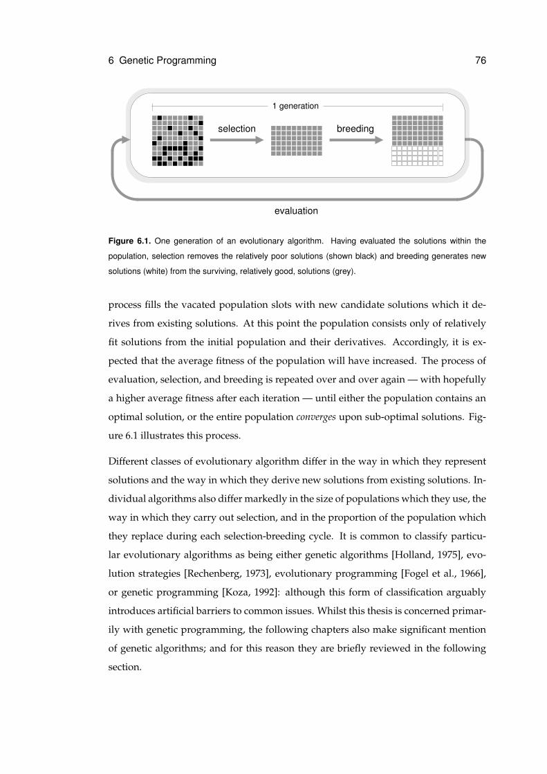
6 Genetic Programming 76
selection breeding
evaluation
1 generation
Figure 6.1. One generation of an evolutionary algorithm. Having evaluated the solutions within the
population, selection removes the relatively poor solutions (shown black) and breeding generates new
solutions (white) from the surviving, relatively good, solutions (grey).
process fills the vacated population slots with new candidate solutions which it de-
rives from existing solutions. At this point the population consists only of relatively
fit solutions from the initial population and their derivatives. Accordingly, it is ex-
pected that the average fitness of the population will have increased. The process of
evaluation, selection, and breeding is repeated over and over again — with hopefully
a higher average fitness after each iteration — until either the population contains an
optimal solution, or the entire population converges upon sub-optimal solutions. Fig-
ure 6.1 illustrates this process.
Different classes of evolutionary algorithm differ in the way in which they represent
solutions and the way in which they derive new solutions from existing solutions. In-
dividual algorithms also differ markedly in the size of populations which they use, the
way in which they carry out selection, and in the proportion of the population which
they replace during each selection-breeding cycle. It is common to classify particu-
lar evolutionary algorithms as being either genetic algorithms [Holland, 1975], evo-
lution strategies [Rechenberg, 1973], evolutionary programming [Fogel et al., 1966],
or genetic programming [Koza, 1992]: although this form of classification arguably
introduces artificial barriers to common issues. Whilst this thesis is concerned primar-
ily with genetic programming, the following chapters also make significant mention
of genetic algorithms; and for this reason they are briefly reviewed in the following
section.
6 Genetic Programming 77
6.1.1 Genetic Algorithms
The genetic algorithm (GA) is an evolutionary algorithm which mimics both the repre-
sentation and variation mechanisms of biological evolution. A GA candidate solution
is represented using a linear string in analogy to a biological chromosome. Accord-
ingly, GA practitioners use biological terms to describe the components of candidate
solutions: whereby each position within a GA chromosome is known as a gene locus
(or just a gene) and its value is an allele. Historically, GA chromosomes are fixed
length binary strings (although some GAs use variable length strings and higher-
cardinality alphabets — including real numbers). New solutions are constructed from
existing solutions using operators whose effects resemble the action of mutation and
recombination upon biological chromosomes. Mutation operators randomly change
the allele of a particular gene locus whereas crossover recombines groups of contigu-
ous genes from two or more existing chromosomes. The mechanics of individual GAs
vary considerably. However, most GAs are generational: meaning that the entire pop-
ulation is replaced during each iteration; and most have a selection mechanism that
allocates each solution’s contribution to the next generation roughly in proportion to
its relative fitness in the current generation. Consequently, the best solutions have
their genes well represented in the next generation whilst the worst solutions tend to
give no contribution to the next generation.
Crossover is traditionally considered the dominant search operator in GAs, and mu-
tation is considered a background operator which replenishes genetic diversity lost
during selection. Crossover proceeds as follows: two chromosomes are aligned, a
number of crossover points are selected randomly along the chromosome lengths, and
groups of genes between every other pair of crossover points are swapped between
the two chromosomes. Genetic linkage is said to occur between alleles at different
gene loci that remain together following recombination. Given the way that crossover
works, genetic linkage is most likely to occur between alleles at gene loci which have
proximal positions within the chromosome. This means that GAs must function as
a result of propagating small groups of alleles found close together within chromo-
somes: groups that are known as building blocks within the GA literature [Goldberg,
1989]. However, this is only useful if chromosomal building blocks correspond to
building blocks found within the problem domain. If this is not the case, or partic-
6 Genetic Programming 78
ularly if the problem’s building blocks are represented by groups of highly spaced
alleles, performance is likely to be impaired. Such problems can sometimes be solved
by re-arranging gene loci within the chromosome. GAs which do this automatically
are known as linkage learning GAs and are discussed in section 7.5.
6.2 Conventional Genetic Programming
Genetic programming (GP) is a generic term used to mean an evolutionary computa-
tion system which is used to evolve programs. Early forms of GP can be traced back
to Friedberg [1958] and Cramer [1985]. The first GP system to bear the name ‘Ge-
netic Programming’ was devised by Koza1 [Koza, 1992]; and this, by virtue of being
the first successfully applied and widely recognised form of GP, forms the basis of
conventional GP systems.
Koza’s genetic programming represents programs by their parse trees. A parse tree is
a tree-structure which captures the executional ordering of the functional components
within a program: such that a program output appears at the root node; functions are
internal tree nodes; a function’s arguments are given by its child nodes; and termi-
nal arguments are found at leaf nodes. A parse tree is a particularly natural structure
for representing programs in LISP; the language Koza first used for genetic program-
ming. This is one reason why the parse tree was chosen as a representation for genetic
programming. A problem, in GP, is specified by a fitness function, a function set, and
a terminal set. The function and terminal sets determine from which components a
program may be constructed; and the fitness function measures how close a particu-
lar program’s outputs are to the problem’s required outputs. The initial population
is filled with programs constructed randomly from components in the function and
terminal sets2.
Conventional GP derives new programs from existing programs using three differ-
ent methods. Point mutation randomly changes the functions or terminals found at
a proportion of the nodes within a parse tree. The number of nodes to be mutated
1Hence the term genetic programming is also sometimes used to refer to versions of Koza’s GP used toevolve entities other than programs: for example, engineering structures; some of which can be describedwith the same representation that Koza’s GP uses to represent programs.
2Although in most implementations, the programs in the initial population are biased towards certainshapes and sizes in order to maximise search space coverage.
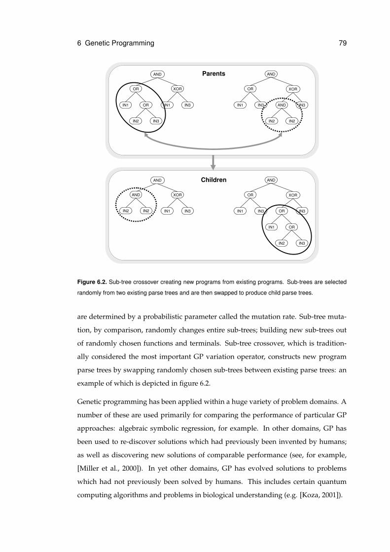
6 Genetic Programming 79
ORIN1
IN3IN2
AND
IN2IN2
ORIN1
IN3IN2
XOR
IN3IN1
AND
OR
IN1 IN3AND
IN2IN2
IN3
AND
OR
IN1 IN3IN3
XOR
IN3IN1
Parents
Children
AND
XOR
XOR
AND
OR
OR
Figure 6.2. Sub-tree crossover creating new programs from existing programs. Sub-trees are selected
randomly from two existing parse trees and are then swapped to produce child parse trees.
are determined by a probabilistic parameter called the mutation rate. Sub-tree muta-
tion, by comparison, randomly changes entire sub-trees; building new sub-trees out
of randomly chosen functions and terminals. Sub-tree crossover, which is tradition-
ally considered the most important GP variation operator, constructs new program
parse trees by swapping randomly chosen sub-trees between existing parse trees: an
example of which is depicted in figure 6.2.
Genetic programming has been applied within a huge variety of problem domains. A
number of these are used primarily for comparing the performance of particular GP
approaches: algebraic symbolic regression, for example. In other domains, GP has
been used to re-discover solutions which had previously been invented by humans;
as well as discovering new solutions of comparable performance (see, for example,
[Miller et al., 2000]). In yet other domains, GP has evolved solutions to problems
which had not previously been solved by humans. This includes certain quantum
computing algorithms and problems in biological understanding (e.g. [Koza, 2001]).
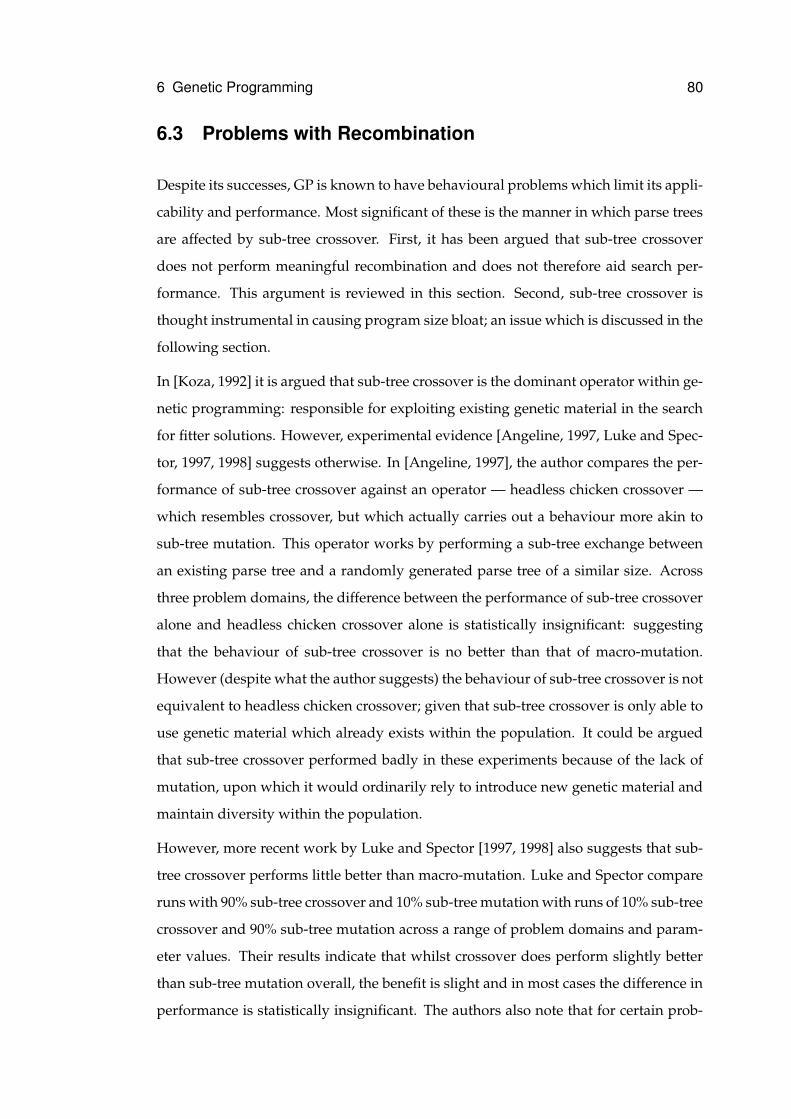
6 Genetic Programming 80
6.3 Problems with Recombination
Despite its successes, GP is known to have behavioural problems which limit its appli-
cability and performance. Most significant of these is the manner in which parse trees
are affected by sub-tree crossover. First, it has been argued that sub-tree crossover
does not perform meaningful recombination and does not therefore aid search per-
formance. This argument is reviewed in this section. Second, sub-tree crossover is
thought instrumental in causing program size bloat; an issue which is discussed in the
following section.
In [Koza, 1992] it is argued that sub-tree crossover is the dominant operator within ge-
netic programming: responsible for exploiting existing genetic material in the search
for fitter solutions. However, experimental evidence [Angeline, 1997, Luke and Spec-
tor, 1997, 1998] suggests otherwise. In [Angeline, 1997], the author compares the per-
formance of sub-tree crossover against an operator — headless chicken crossover —
which resembles crossover, but which actually carries out a behaviour more akin to
sub-tree mutation. This operator works by performing a sub-tree exchange between
an existing parse tree and a randomly generated parse tree of a similar size. Across
three problem domains, the difference between the performance of sub-tree crossover
alone and headless chicken crossover alone is statistically insignificant: suggesting
that the behaviour of sub-tree crossover is no better than that of macro-mutation.
However (despite what the author suggests) the behaviour of sub-tree crossover is not
equivalent to headless chicken crossover; given that sub-tree crossover is only able to
use genetic material which already exists within the population. It could be argued
that sub-tree crossover performed badly in these experiments because of the lack of
mutation, upon which it would ordinarily rely to introduce new genetic material and
maintain diversity within the population.
However, more recent work by Luke and Spector [1997, 1998] also suggests that sub-
tree crossover performs little better than macro-mutation. Luke and Spector compare
runs with 90% sub-tree crossover and 10% sub-tree mutation with runs of 10% sub-tree
crossover and 90% sub-tree mutation across a range of problem domains and param-
eter values. Their results indicate that whilst crossover does perform slightly better
than sub-tree mutation overall, the benefit is slight and in most cases the difference in
performance is statistically insignificant. The authors also note that for certain prob-
6 Genetic Programming 81
ORIN1
IN3IN2
XOR
IN3IN1
AND
OR
AND
IN2IN2
XOR
IN3IN1
AND
AND
AND
AND
OR
IN1 IN3AND
IN2IN2
IN3
XOR
Figure 6.3. Loss of context following sub-tree crossover.
lems (including symbolic regression), crossover performs better for large populations
and few generations whilst sub-tree mutation performs better for small populations
and large numbers of generations. However, this does not hold for all problems.
This poor performance has perhaps less to do with crossover than it has to do with
the parse tree representation. For GAs, it is fairly well accepted that crossover im-
proves performance for problem domains with reasonably low levels of epistasis and
with a reasonable arrangement of genes within a chromosome i.e. in situations where
building blocks can be readily processed by crossover. After all, recombination is log-
ically a useful operation — it enables co-operative evolution by allowing information
exchange within a population. Furthermore, it appears to play a primary role within
eukaryotic evolution.
Sub-tree crossover is a natural recombination operator for parse trees. However, by
exchanging randomly chosen sub-trees between programs, it does not carry out a log-
ically meaningful operation. This is illustrated in figure 6.3. In this example, a ran-
dom sub-tree is selected in an existing parse tree and is replaced by a sub-tree which
is randomly selected from another parse tree. These parent parse trees have signif-
icant shared behaviours: both apply an AND function to the outputs of OR and XOR
functions, and both have a left-hand branch which calculates the OR of a number of
6 Genetic Programming 82
input terminals; so in principal it would seem that they have compatible informa-
tion to share. However, because the exchanged sub-trees are selected from different
positions and have different size, shape and functionality, the behaviour of the result-
ing child solution bears little resemblance to either parent. The behaviour of each of
these programs is determined by the output of the AND function at the top of the pro-
gram. The output of a function depends upon both the function it applies and upon
its input context: the inputs to which it applies the function. Consequently, if its input
context changes considerably, then so does its output. Given that most possible pro-
grams will generate very poor solutions to a problem, and that the parent programs
are presumably relatively good at solving the problem, a considerable change in out-
put behaviour is likely to result in a program with low fitness. In the example, one of
the AND function’s inputs changes from being the OR of three inputs to the AND of a
single input with itself: leading to a significant change in output behaviour.
Since it is unlikely that sub-tree crossover will exchange sub-trees with similar posi-
tion, size, shape, or behaviour, most GP sub-tree crossovers will lead to child programs
which are considerably less fit than their parents. In essence, this happens because a
component’s context is recorded in terms of its position within a parse tree; and be-
cause sub-tree crossover does not preserve the positions of components. Later in this
thesis it will be argued that this failing is as much the fault of the program’s represen-
tation as it is the fault of the sub-tree crossover operator.
6.4 Solution Size Evolution and Bloat
Parse trees are variable length structures and, in the absence of any mechanisms of
constraint, may change size freely during the course of evolution. Unfortunately, in
GP there is a tendency for parse trees to grow, rather than shrink, over time. This
leads to a phenomenon called bloat whereby programs become larger and larger with-
out significant improvement in function. In standard GP, program bloat has nearly
quadratic complexity [Langdon, 2000a]. This causes a number of problems. First, it
places a strain on both storage and executional resources. Second, it leads to programs
which are large, complex, inefficient and hard to interpret. Third, bloat usually takes
the form of an increase in non-functional code; and given that this code comprises
6 Genetic Programming 83
most of the program, it becomes the target of most crossover and mutation events:
protecting the functional code from change and ultimately reducing the effectiveness
of evolution. The role of non-functional code in GP is discussed in more detail in sec-
tion 7.4.1. Although the exact cause of bloat is not known, a number of mechanisms
have been identified which appear to contribute to the effect. These are replication
accuracy, removal bias, search space bias, and operator bias; and are discussed below.
The replication accuracy theory of bloat [Blickle and Thiele, 1994, McPhee and Miller,
1995, Nordin and Banzhaf, 1995] follows from the protective role of non-functional
code outlined above. Large programs containing a lot of non-functional code are more
likely to survive crossover or mutation with no change to their function than smaller
programs or programs with less non-functional code. Therefore, these programs have
a higher replication accuracy. Given that their behaviour is less likely to change as a
result of crossover; and given that behavioural changes resulting from crossover tend
to be negative; these programs are more likely to be the parents of viable children; and
hence will become better represented in the next generation than smaller programs
and programs with less non-functional code. Consequently, there is selective pressure
for programs to become larger. Furthermore, child programs derived from programs
with high replication accuracy are themselves likely to be good replicators (they have
high effective fitness, to use Banzhaf et al.’s [1998] terminology) and will pass this trait
on to their descendants.
The removal bias theory of bloat [Soule et al., 1996] also appeals to the disruptive effect
of sub-tree crossover. Following crossover, the behaviour of a child program is more
likely to be like its parent (and therefore more likely to be viable) if the sub-tree being
replaced occurs near the bottom of the parent parse tree. This is because: (a) compo-
nents lower in a parse tree have less influence upon the program’s outputs; and (b)
non-functional code tends to occur at the bottom of parse trees. Consequently, the
sub-tree which is replaced is likely to have below average size. However, there are no
similar constraints upon the size of the sub-tree with which it is replaced; meaning that
the existing sub-tree is more likely to be replaced with a larger sub-tree. Accordingly,
viable child programs are more likely to be larger than their parents.
The search space bias theory of bloat [Langdon and Poli, 1997] does not appeal to the be-
haviour of variation operators. To use Langdon and Poli’s [2002] own words: ”above
6 Genetic Programming 84
a certain size threshold there are exponentially more longer programs of the same
fitness as the current program than there are of the same length (or shorter).” Accord-
ingly, it is more likely that evolutionary search will explore those programs which
are longer than those which are of the same length or shorter. A similar argument is
made by Miller [2001], who believes that bloat is caused by evolution exploring a pro-
gram’s neutral variants: most of which will be larger than the existing program. The
operator bias theory of bloat suggests that certain variation operators aggravate this ef-
fect through innate imbalances which cause them to sample larger programs (see, for
example, [McPhee and Poli, 2001]).
6.5 Expressiveness
Expressiveness is the capacity for a representation to express appropriate programs.
Evolvability is the capacity for a representation to evolve appropriate programs. For
GP, these two issues are related: it is not possible to evolve a program which can not be
expressed and it is not possible to express a program if it can not be evolved by the GP
system. Clearly, both of these issues are important. For GP to be successful, it must be
able to both search the appropriate region of the search space, i.e. express programs in
that region; and be able to get to the appropriate region of the search space from those
areas covered by an arbitrary starting population, i.e. evolve programs in that region.
Furthermore (and certainly in the software engineering community), expressiveness is
seen as a property which encourages evolvability; since if a program can be expressed,
it can also be evolved by making a certain number of changes to an existing program.
Nevertheless, expressiveness in itself is not sufficient to produce evolvability; since
although it may make it possible to evolve a certain program, it does not necessarily
make it easy to evolve the program.
Despite these relations, in GP research expressiveness and evolvability are often treated
as different, sometimes conflicting, design goals. Improving expressiveness can in-
crease the scope of GP by making it possible to evolve a greater range of programs or
particular types of programs. However, in doing so it changes the search space of GP;
and this can make it harder to evolve a program to solve a particular problem. Indeed,
for a particular kind of problem, there is probably a trade-off between the expressive-
6 Genetic Programming 85
ness of the representation and its evolvability — even though in practice a knowledge
of the problem domain would be required to make this trade-off.
Nonetheless, expressiveness is an important topic in GP and it does share a number
of issues in common with the study of evolvability in GP. In recognition of these facts,
this section provides a flavour of some of the approaches which have been taken to
improve the expressiveness of GP. However, it does not attempt to be an exhaustive
reference and, although the issue of evolvability is discussed at length in the next chap-
ter, it does not attempt to artificially separate the concerns of expressive and evolvable
representations.
So far the term representation has been used somewhat generically to refer to the way
in which a program is presented to the evolutionary mechanism of the GP system.
For the remainder of this chapter, the term is used in a more restricted sense to mean
the format or structure of the program rather than the language it is written in. The
term representational language (taken from Altenberg [1994]) is used to refer to the lan-
guage within which a program is expressed. This section is organised into two parts;
separating those approaches which are primarily motivated by a desire to change the
representational language from those which are primarily motivated by a desire to
change the representation of GP.
6.5.1 Linguistic Approaches
This section introduces a selection of GP approaches which use languages or linguistic
elements not normally found in GP. The section is split into three parts. The first
part introduces techniques which introduce a notion of type to GP. The second part
discusses the relative merits of using memory and state within GP. The third part
presents GP systems which use particular kinds of programming language.
Type Systems
The use of type systems to limit evolutionary and genetic behaviours was first ex-
plored by Koza [1992] in the form of constrained syntax structures. Most GP systems
are based around the idea of closure: that all data within a program can be inter-
changed freely between nodes; constraining the data to be of one type. Introducing
6 Genetic Programming 86
typed data involves re-writing tree generation and genetic operator routines such that
generated and modified programs always obey the rules of the type system. Koza’s
ideas were extended in [Montana, 1994, 1995] by Strongly-Typed GP (STGP), a sys-
tem allowing variables, constants, function argument and return values to be of any
type, so long as the exact types are defined in advance. Generic functions were intro-
duced as a means of avoiding re-writing functions for each data type. When used in a
program, these are instantiated (and remain instantiated) with typed arguments and
return values.
By introducing type constraints and limiting evolution to generating legal trees, STGP
significantly reduces the search space. In Montana’s experiments, STGP was shown to
produce superior results to standard GP across a range of moderately hard problems.
This form was reproduced in [Haynes et al., 1996], where STGP was applied to a diffi-
cult agent-cooperation problem. The programs evolved were significantly better than
those produced by GP. In addition to being more effective, the STGP programs also
demonstrated greater generality and readability. The reduced search space meant that
they evolved significantly faster than standard GP programs. However, this reduced
search space also suggests potential problems in domains where the optimal solution
is outside of the constraints imposed by the type system. Here, STGP will not find the
optimum, and it will not be obvious in advance whether the optimum can be found
by STGP.
Another approach to introducing types to GP can be found in Spector’s [Spector, 2001,
Spector and Robinson, 2002] PushGP; a form of GP based upon Spector’s custom-
designed Push language3. Push is a stack-based language which maintains separate
stacks for data of different types. Functions, whilst generic, operate upon arguments
at the top of whichever stack is currently identified by the system’s TYPE stack; a
special stack which contains type references. Programs comprise a linear sequence of
arguments and functions. Because the stack system de-couples arguments from the
functions which use them, it is no longer possible to apply incorrectly-typed argu-
ments to a function; and therefore there is no need to use special syntax-preserving
recombination operators. PushGP performs better than GP upon even-n-parity prob-
3The Push language is actually designed to support auto-constructive evolution systems, such asPushpop, in which programs describe and evolve their own reproduction operators. However, this workis outside the scope of this thesis.
6 Genetic Programming 87
lems where n > 5; and, more importantly, scales considerably better for increasing n
that either standard GP or GP with ADFs (Automatically Defined Functions; which
are introduced in section 7.3.1).
Memory and State
Conventional GP has no explicit notion of state. The problems it handles are func-
tional or reactive, based upon simple mappings from input to output. Adding state
allows GP to solve harder knowledge-based problems. The earliest attempt at state
was Koza’s progn statement, implicitly handling state via side-effecting terminals.
State can be represented explicitly within programs using either abstract variables or
indexed memory. Indexed memory, in particular, introduces Turing completeness:
and is the motivation behind an approach described by Teller [1994, 1996].
Teller defines memory as an array of integer-holding locations, M -locations wide and
holding numbers between 0 and M . The use of M for both limits prevents evolving
programs from using out-of-range values, since a stored number might be used as an
index elsewhere in the program (and vice versa). This is simpler, and more natural,
than normalising out-of-range numbers. To handle memory-access, two extra non-
terminals are placed into the function set. READ(Y) returns the value at address Y in
the memory. WRITE(X,Y) places X at address Y, returning the previous value of Y.
The low-level approach taken by this strategy means that no constraints are placed
on how memory should be used, and in theory allows the emergence of more ad-
vanced memory models such as indirection. Teller found a 600% improvement in
performance over conventional GP when he applied this system to a problem requir-
ing state information. However, optimal performance is only achieved if the memory
is the right size for the problem. If M is too small, then either there is too little state
space or the state variables become too close together in memory4. If M is too large,
then information is easily lost because there is little chance of a read and a write using
the same memory location.
In [Langdon, 1995], Teller’s scheme is used to evolve data structures. More recently,
4This is called the ‘tight representation problem’, usually found in codes when adjacent states havevery different representations. For instance, in binary 7 (0111) is very different to 8 (1000). A similarproblem occurs here when state components are forced too close together. Introducing redundancy, inboth indexed memory and in codes, alleviates this problem.
6 Genetic Programming 88
Spector and Luke [1996] have taken Teller’s indexed memory and used it to confer
a notion of culture within an evolving GP system. Culture is the non-genetic trans-
fer of information between individuals. In natural systems, this provides a means of
communication, both within and across generations, which is faster and more open
than normal genetic evolution. In this approach, culture is expressed as a common
indexed memory which any member of any generation can access using Teller’s stan-
dard functions. Spector found the use of culture to improve performance upon a range
of reactive problems. In theory, culture should allow various co-operative or compet-
itive strategies to evolve. Furthermore, it allows an individual to communicate with
itself across generations and even across fitness cases. Spector also noted that, for all
the reactive problems he tried, Teller’s GP performed worse than standard GP with-
out memory; suggesting that memory should only be used for problems which cannot
be solved without it. Presumably this is due to the increased size of the search space
caused by the presence of the extra READ and WRITE functions.
Language
A number of GP systems attempt to evolve programs in specific languages, or spe-
cific types of language. Yu [Yu and Clack, 1998, Yu, 1999], for instance, describes a
GP system based upon a functional programming approach. The motivation behind
this approach was to make use of the implicit structural abstraction available within
functional languages. Structure abstraction is based upon the use of higher-order func-
tions; a motif common in functional programming where a function is passed as an
argument to another function. The function passed is defined as a λ-abstraction: an
anonymous reusable module. By introducing a minimal type system, crossover is
forced to preserve the bi-layer λ-abstraction/higher-order function motif. Structure
abstraction occurs because genetic manipulation still allows the content of both layers
to change. During evolution, λ-abstractions are generated dynamically. Higher-order
functions typically apply a λ-abstraction recursively over a data structure; an effect
called implicit recursion. This high-level behaviour, linked to controlled use of recur-
sion, allows the complexity of some hierarchical problems to be reduced to a simple
linear problem; though the success of this approach depends upon user-definition of
appropriate higher-order functions.
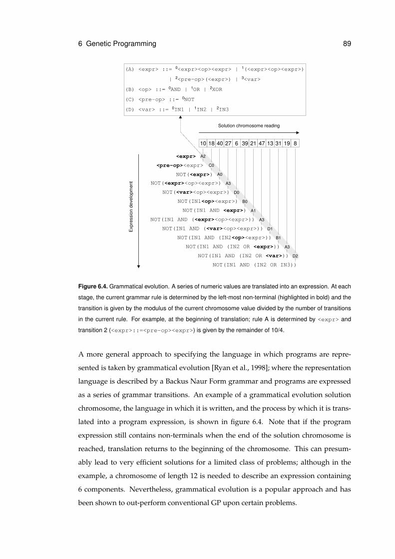
6 Genetic Programming 89
(A) <expr> ::= 0<expr><op><expr> | 1(<expr><op><expr>)
| 2<pre-op>(<expr>) | 3<var>
(B) <op> ::= 0AND | 1OR | 2XOR
(C) <pre-op> ::= 0NOT
(D) <var> ::= 0IN1 | 1IN2 | 2IN3
<pre-op><expr>
NOT(<expr>)
A2
C0
NOT(<expr><op><expr>)
A0
NOT(<var><op><expr>)
A3
NOT(IN1<op><expr>)
D0
NOT(IN1 AND <expr>)
B0
NOT(IN1 AND (<expr><op><expr>))
A1
NOT(IN1 AND (<var><op><expr>))
A3
NOT(IN1 AND (IN2<op><expr>))
D1
NOT(IN1 AND (IN2 OR <expr>))
B1
NOT(IN1 AND (IN2 OR <var>))
A3
NOT(IN1 AND (IN2 OR IN3))
D2
10 18 40 27 6 39 21 47 13 31 19 8
<expr>
Solution chromosome readingE
xpre
ssio
n de
velo
pmen
t
Figure 6.4. Grammatical evolution. A series of numeric values are translated into an expression. At each
stage, the current grammar rule is determined by the left-most non-terminal (highlighted in bold) and the
transition is given by the modulus of the current chromosome value divided by the number of transitions
in the current rule. For example, at the beginning of translation; rule A is determined by <expr> and
transition 2 (<expr>::=<pre-op><expr>) is given by the remainder of 10/4.
A more general approach to specifying the language in which programs are repre-
sented is taken by grammatical evolution [Ryan et al., 1998]; where the representation
language is described by a Backus Naur Form grammar and programs are expressed
as a series of grammar transitions. An example of a grammatical evolution solution
chromosome, the language in which it is written, and the process by which it is trans-
lated into a program expression, is shown in figure 6.4. Note that if the program
expression still contains non-terminals when the end of the solution chromosome is
reached, translation returns to the beginning of the chromosome. This can presum-
ably lead to very efficient solutions for a limited class of problems; although in the
example, a chromosome of length 12 is needed to describe an expression containing
6 components. Nevertheless, grammatical evolution is a popular approach and has
been shown to out-perform conventional GP upon certain problems.
6 Genetic Programming 90
6.5.2 Representational Approaches
This section describes three different, yet related, approaches to adapting the repre-
sentation of evolving programs in GP. The first approach involves changing the archi-
tecture of the program. The second targets the executional structure of programs. The
third uses developmental representations.
Program Architecture
Perhaps the simplest adaptation of the standard GP representation is to use a graph
rather than a tree to express the connectivity of a program. PDGP (Parallel Distributed
Genetic Programming) [Poli, 1997] and cartesian GP [Miller and Thomson, 2000] both
take this approach: representing a program as a directed graph in which each node
is either a function or a terminal. Both systems have significant commonality: both
have mechanisms to prevent cycles (when appropriate) and both allow nodes to exist
in the representation but not have any connections to other nodes (the significance of
which is discussed in section 7.4.3). However, the motivation behind these systems is
different. PDGP aimed to use a program model which reflects the kind of distributed
processing that occurs in neural networks. Cartesian GP was originally designed to
evolve both the functionality and routing of circuits on FPGAs: requiring a represen-
tation in which components were laid out on a grid — and which incidentally could
be interpreted as a graph structure. Both methods show performance improvement
within certain problem domains; and both tend to evolve smaller, more efficient, pro-
grams (a behaviour which is discussed in more detail in section 7.3.2).
A number of GP systems [Angeline, 1998a, Silva et al., 1999, Ferreira, 2001] take a two-
layer approach to representation in which one layer describes a collection of parse
trees and a higher layer describes how these parse trees interact to perform some uni-
fied processing. The earliest of these is Angeline’s MIPs (Multiple Interacting Pro-
grams) [Angeline, 1998a] representation. A MIPs net (named to reflect its structural
similarity to a neural network) can be interpreted as a graph in which each node cor-
responds to a parse tree. A number of nodes are designated output nodes; and the
outputs of their corresponding parse trees determine the output behaviour of the pro-
gram. Connections between nodes are realised by references to the outputs of other

6 Genetic Programming 91
nodes appearing internal to parse trees. In theory, these connections may be feed-
forward or recurrent and have synchronous or asynchronous updates; although Ange-
line limited his experiments to synchronous recurrent MIPs nets. Applied to a number
of problems, his approach demonstrated better performance and better solution gen-
erality. Applied to a problem whose solution required memory, the system evolved
a particularly efficient solution which made use of the representation’s implicit abil-
ity to store state. Similar observations have been made by Silva et al. [1999] in the
context of their Genetically Programmed Network approach; which uses a represen-
tation broadly similar to Angeline’s MIPs representation. Ferreira’s GEP (Gene Ex-
pression Programming) [Ferreira, 2001] also makes use of multiple parse trees; though
the meaning and connectivity of these parse trees is determined by the fitness func-
tion and is not evolved by the system. Perhaps what is most interesting about GEP is
the way in which parse trees are encoded: a pre-fix variant which the author believes
to be particularly supportive of variation operators. GEP also shows significant per-
formance gains over standard GP (although the author’s ‘marketing’ style of writing
makes it hard to work out exactly why this is the case): and is the only one of these ap-
proaches to have had a notable impact on the GP community; even though the other
two approaches are perhaps more behaviourally interesting.
Executional Structure
Many of the GP systems introduced in section 6.5.2 use representations which implic-
itly change the manner in which a program’s executional structure is represented. In
conventional GP, the effect of a component upon execution is determined by its loca-
tion within a parse tree. By comparison, in PushGP there is considerable decoupling
between the location of an instruction or argument in the representation and its tem-
poral role within the program’s execution. This occurs because arguments and results
can be stored within stacks and used later; or even not be used at all. A similar argu-
ment applies to other forms of GP which use linear representations; such as AIMGP5
(Automatic Induction of Machine Code with Genetic Programming) [Nordin, 1994]
which represents programs as a sequence of machine code instructions, each of which
5AIMGP and its predecessors were originally developed to make the evaluation phase of GP faster.Nevertheless, such approaches also have benefits for evolvability. These are discussed in proceedingchapters.
6 Genetic Programming 92
is able to save and load values from register locations. In this case the registers provide
the means for decoupling instruction location from instruction behaviour. In fact, any
form of memory or state within any kind of representation can have some effect upon
the executional structure of a program: although in representations such as parse trees
this effect is relatively small.
Whilst for most representations executional ordering emerges implicitly from the con-
nectivity and behaviour of components, some GP systems use representations which
express execution ordering explicitly. PADO (Parallel Algorithm Discovery and Or-
chestration) [Teller and Veloso, 1996] is a complex learning system based upon the
principles of genetic programming. PADO uses a graph-based representation in which
each node describes some processing behaviour and, depending on the result, carries
out some judgement behaviour which decides which outgoing path execution will
continue along. Unlike normal GP, which typically describes fixed expressions, PADO
describes structures which are much more akin to computer programs: containing
complex flows of execution which depend upon the results of internal calculations.
PADO has been used for object recognition tasks, giving an impressive level of perfor-
mance. GNP (Genetic Network Programming) [Katagiri et al., 2000, Hirasawa et al.,
2001] is a GP approach with a similar representation to PADO; but which also ex-
presses delays within and between program nodes. GNP is used to model complex
dynamical systems; out-performing conventional GP on a complex ant-foraging prob-
lem [Hirasawa et al., 2001].
Developmental Representations
For most of the approaches described above, a program’s representation directly de-
scribes a program. A developmental representation, by comparison, describes how
a program or other artifact is constructed. It only indirectly describes what is con-
structed. In the long term, it would seem that development is key to overcoming the
problems currently associated with scalability in evolutionary computation. For di-
rect (non-developmental) GP encodings, representation length is proportional to pro-
gram length. Typically this means that representation length grows in proportion to
problem difficulty, and typically this means an above-linear rise in the time and space
required for evolutionary search — not to mention the fact that the time required to
6 Genetic Programming 93
evaluate solutions also often grows at an above-linear rate. With developmental en-
codings, however, representation length normally grows at a below-linear rate rela-
tive to program length: and consequently could lead to better scalability and better
evolutionary performance. However, developmental representations for evolution-
ary computation are still in their relative infancy and are yet to show a demonstrable
performance advantage. Nevertheless, research in this area has led to a number of
interesting ideas and some promising insights.
Developmental representations are based around the idea of re-writing systems: start-
ing from some initial configuration, a series of re-writing rules transforms this con-
figuration through a number of steps which eventually lead to the developed arti-
fact. Grammatical evolution is a simple example of this approach. However, many
approaches are modelled upon biological growth processes [Boers and Kuiper, 1992,
Gruau, 1994, Koza et al., 1999, Haddow et al., 2001, Downing, 2003, Miller and Thom-
son, 2003]. A number of these have been applied to genetic programming (especially
circuit evolution) [Haddow et al., 2001, Downing, 2003, Koza et al., 1999, Miller and
Thomson, 2003]. Miller and Thomson [2003] use a developmental model in which a
single starting ‘cell’ is iteratively replicated to generate a pattern of interacting cells in
which both the pattern of interaction and the behaviour of each cell is decided by a sin-
gle evolved cartesian GP program. Following development, the cellular pattern is in-
terpreted as a digital circuit where interactions represent wires and cellular behaviours
represent gates. Whilst distinctly unsuccessful from a performance perspective, this
system is apparently capable of evolving partially generalised solutions to the even-
n-parity problem; where n is determined by the number of iterations allowed during
circuit development.
Downing [2003] describes a developmental program representation based upon Spec-
tor’s Push language (described in section 6.5.1). In Downing’s approach, which is
based upon a cellular colony metaphor, both development and execution are deter-
mined by a single Push program. Each cell has its own code and data stacks. The
generation of new cells and interaction between cells is achieved through special lan-
guage primitives. Inter-cell communication is achieved through primitives that re-
direct function outputs to stacks in other cells. Downing gives examples of how par-
ticular Push programs lead to emergent processing behaviours within the resulting
6 Genetic Programming 94
cellular ecologies. Whilst intended to be used within an EC framework, results re-
garding evolutionary behaviour and performance have yet to be published.
6.6 Summary
Genetic programming (GP) is an evolutionary computation approach to automatic
programming: using a computational model of evolution to design and optimise com-
puter programs and other executable structures. GP is mechanistically similar to the
genetic algorithm and other population based search algorithms. Whilst GP has been
successfully applied within a wide range of problem domains, the method has certain
behavioural problems which limit its performance and scalability. Perhaps the most
significant of these is the failure of its recombination operator, sub-tree crossover, to
carry out meaningful recombination; limiting the capacity for co-operative interac-
tions between members of the population. Sub-tree crossover is also thought to play
a substantial role in the un-controlled program size growth phenomenon known as
bloat.
In addition to reviewing conventional GP, this chapter has introduced a selection of
derivative GP approaches which attempt to improve the behaviour or scope of pro-
gram evolution by increasing the expressiveness of the representation used to rep-
resent programs. The next chapter continues this look at derivative GP approaches
by presenting a range of techniques which aim to improve the evolvability of the GP
program representation.
7 Evolvability in EvolutionaryComputation
This chapter is a review of research aimed at improving the evolvability of the artefacts
which are evolved by evolutionary computation techniques. In particular, it attempts
to address those issues which are of special relevance to genetic programming. Where
appropriate, this includes research done in other fields of evolutionary computation.
7.1 Variation versus Representation
In Chapter 1, evolutionary change was described as the result of sources of variation
acting upon the representation of an entity. From this it follows that the nature of evo-
lutionary change might be improved by either (i) improving the ability of variation to
enact appropriate change; or (ii) improving the ability of the representation to accept
appropriate change. Both of these are valid. Nevertheless, in this thesis, emphasis is
clearly placed upon the second of these approaches. This is for two reasons.
First, whilst variation mechanisms are an important part of biological evolution, their
behaviours appear relatively simple when compared to the rich organisation, devel-
opmental mechanisms, and behavioural scope of biological representations. Even
recombination, which is under evolutionary control, carries out a non-deterministic
behaviour whose evolutionary effect is determined primarily by the response of the
representation. In looking for biological guidance concerning evolvability it would
seem, therefore, that more information could be gleaned by looking at biological rep-
resentations rather than the sources of variation within biological evolution.
95
7 Evolvability in Evolutionary Computation 96
Secondly, it is common knowledge in computer science that if the same effect can
be achieved by improving the way information is represented or by improving the
way information is operated upon, better generality can be achieved by adapting the
representation. For instance, if the information in a database is structured in a way
that makes certain information difficult to manipulate, it would be considered better
in the long run to improve the way the database is structured rather than improve
the complexity of queries used to manipulate the information. Likewise, in the first
instance it would seem better in the long run to change the way an evolving entity
is represented rather than the way in which it is manipulated if both are capable of
improving the way that it evolves.
Nevertheless, some interesting work has been done in adapting variation operators.
This is briefly reviewed in the next section. The remaining sections of this chapter
are concerned with existing approaches to improving the evolvability of representa-
tions. These are organised according to the manner in which they attempt to introduce
evolvability: through pleiotropy, redundancy or removal of positional bias. In part
this requires some familiarity with information from the previous chapter and from
Chapter 5.
7.2 Adapting Variation
In the last chapter, the relative failure of sub-tree crossover in genetic programming
was attributed to the unlikelihood of it carrying out meaningful recombinative be-
haviours. A number of researchers [Poli and Langdon, 1997, Langdon, 1999, 2000b,
Francone et al., 1999, Hansen, 2003a] have looked at the possibility of constraining
the behaviour of GP crossover in order to prevent inappropriate behaviours. This
has led to a range of homologous crossover operators which attempt to limit genetic
exchange to regions of genetic homology. One-point crossover [Poli and Langdon,
1997, 1998], which resembles GA one-point crossover, does this by identifying and
using a crossover point which occurs in the same position within both parent parse
trees. Uniform crossover [Poli and Langdon, 1998] models GA uniform crossover by
identifying regions of common position and shape within both parents and uniformly
recombining the nodes within these regions. However, neither of these operators lead
7 Evolvability in Evolutionary Computation 97
to a significant increase in performance and both introduce a considerable processing
overhead in identifying homologous regions. Size-fair crossover [Langdon, 1999] uses
a different approach and only constrains sub-tree crossover to sub-trees of equal size,
though again produces little increase in performance. More recently, Langdon [2000b]
has extended this approach by using a formal definition of genetic distance based
upon location and size to determine where crossover events may occur. This has pro-
duced more encouraging results, although requiring more computational overhead
during crossover.
The only homologous recombination operator to produce a sizeable improvement in
performance is Francone et al’s [1999] sticky crossover which works on linear GP
programs. Sticky crossover is a relatively simple homologous operator which limits
recombination to groups of instructions with common offsets and common lengths.
Francone et al. believe that sticky crossover leads to programs with better general-
ity and higher robustness than standard linear GP programs. Hansen [2003a] shows
that sticky crossover offers superior performance across a wide range of regression
problems and that the resulting programs contain lower incidences of intronic code
(see section 7.4.1 for a definition of intronic code). The relative failure and complexity
of tree GP homologous crossover operators when compared to sticky crossover tends
to suggest that the linear GP program representation is innately more amenable to
meaningful recombination than the parse tree structure of standard GP.
7.3 Introducing Pleiotropy
Recall from section 5.1 that compartmentalisation is the limitation of interactions be-
tween different sub-systems. In the context of biological systems, it was suggested
that compartmentalisation introduces de-constraint: allowing sub-systems to evolve
independently. Nevertheless, it is also believed that pleiotropy — the sharing of genes
between sub-systems; conceptually the opposite of compartmentalisation — plays an
important role by way of reducing the need to re-evolve the same functionality in
different sub-systems. Tree-structured GP representations, by default, confer com-
plete compartmentalisation to the programs they represent: since every function and
terminal instance is involved in exactly one sub-expression. However, given limited
7 Evolvability in Evolutionary Computation 98
availability of time and space, many researchers believe there is virtue in introducing
pleiotropy to GP systems: reducing the time requirement by preventing the need to
re-discover functionality; and reducing the space requirement by preventing the need
to store the same sub-expression at multiple locations in the same program. This sec-
tion introduces two general approaches to introducing pleiotropy to GP: modularity
and implicit reuse.
7.3.1 Modularity
Much of the work on modularity in GP has been carried out by Koza [1992, 1994, 1995].
His earliest work took the form of a ‘define building block’ operator which named sub-
trees and allowed them to be referenced elsewhere in the program as zero-argument
functions [Koza, 1992]. Later, this idea was extended to the notion of automatically-
defined functions (ADFs): argument-taking functions stored in trees which co-evolve
with the main routine [Koza, 1994]. The architecture of the program — the number,
argument-signatures, and hierarchical limits of these modules — has to be chosen
before evolution begins, either by prospective analysis, which requires knowledge of
problem-decomposition; over-specification, sufficient modules for any possible needs;
affordable capacity, since more modules entail more processing; retrospective analy-
sis, from feedback of previous runs; or by evolutionary selection, which uses an initial
population seeded with many different architectures. Results reported in [Koza, 1992]
and [Koza, 1994] suggest that use of ADFs can lead to a considerable decrease in the
time required to solve certain problems. This is especially true for problems, like par-
ity checkers, whose solutions require a high level of functional duplication. ADFs
have also been shown to decrease the size of evolved solutions.
Nevertheless, from an evolutionary perspective, ADFs have distinct limitations. First,
it is not possible for a program’s architecture to evolve. This places a limit upon modu-
larity and, if the initial architecture is not appropriate, may hinder evolution. Second,
there is no obvious mechanism for introducing de-constraint. Change to an ADF will
affect the behaviour of the program at each calling instance. Whilst this may some-
times be appropriate, sometimes it will not. For example, suppose an ADF is called
from two different sub-trees in a program and, so far, the functionality of the ADF
has been beneficial to the behaviour of both sub-trees. Now suppose that in order
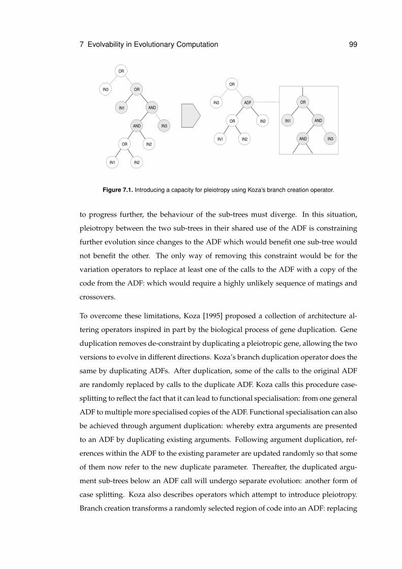
7 Evolvability in Evolutionary Computation 99
IN2IN1
IN2IN1
IN3
AND
IN2OR
AND
IN3
OR
IN1
OR
IN3
IN2
ADF
OR
OR
AND
AND
IN3
OR
IN1
Figure 7.1. Introducing a capacity for pleiotropy using Koza’s branch creation operator.
to progress further, the behaviour of the sub-trees must diverge. In this situation,
pleiotropy between the two sub-trees in their shared use of the ADF is constraining
further evolution since changes to the ADF which would benefit one sub-tree would
not benefit the other. The only way of removing this constraint would be for the
variation operators to replace at least one of the calls to the ADF with a copy of the
code from the ADF: which would require a highly unlikely sequence of matings and
crossovers.
To overcome these limitations, Koza [1995] proposed a collection of architecture al-
tering operators inspired in part by the biological process of gene duplication. Gene
duplication removes de-constraint by duplicating a pleiotropic gene, allowing the two
versions to evolve in different directions. Koza’s branch duplication operator does the
same by duplicating ADFs. After duplication, some of the calls to the original ADF
are randomly replaced by calls to the duplicate ADF. Koza calls this procedure case-
splitting to reflect the fact that it can lead to functional specialisation: from one general
ADF to multiple more specialised copies of the ADF. Functional specialisation can also
be achieved through argument duplication: whereby extra arguments are presented
to an ADF by duplicating existing arguments. Following argument duplication, ref-
erences within the ADF to the existing parameter are updated randomly so that some
of them now refer to the new duplicate parameter. Thereafter, the duplicated argu-
ment sub-trees below an ADF call will undergo separate evolution: another form of
case splitting. Koza also describes operators which attempt to introduce pleiotropy.
Branch creation transforms a randomly selected region of code into an ADF: replacing
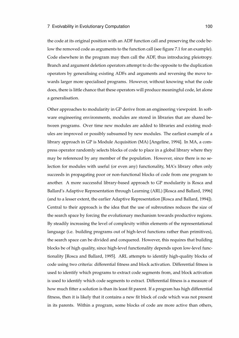
7 Evolvability in Evolutionary Computation 100
the code at its original position with an ADF function call and preserving the code be-
low the removed code as arguments to the function call (see figure 7.1 for an example).
Code elsewhere in the program may then call the ADF, thus introducing pleiotropy.
Branch and argument deletion operators attempt to do the opposite to the duplication
operators by generalising existing ADFs and arguments and reversing the move to-
wards larger more specialised programs. However, without knowing what the code
does, there is little chance that these operators will produce meaningful code, let alone
a generalisation.
Other approaches to modularity in GP derive from an engineering viewpoint. In soft-
ware engineering environments, modules are stored in libraries that are shared be-
tween programs. Over time new modules are added to libraries and existing mod-
ules are improved or possibly subsumed by new modules. The earliest example of a
library approach in GP is Module Acquisition (MA) [Angeline, 1994]. In MA, a com-
press operator randomly selects blocks of code to place in a global library where they
may be referenced by any member of the population. However, since there is no se-
lection for modules with useful (or even any) functionality, MA’s library often only
succeeds in propagating poor or non-functional blocks of code from one program to
another. A more successful library-based approach to GP modularity is Rosca and
Ballard’s Adaptive Representation through Learning (ARL) [Rosca and Ballard, 1996]
(and to a lesser extent, the earlier Adaptive Representation [Rosca and Ballard, 1994]).
Central to their approach is the idea that the use of subroutines reduces the size of
the search space by forcing the evolutionary mechanism towards productive regions.
By steadily increasing the level of complexity within elements of the representational
language (i.e. building programs out of high-level functions rather than primitives),
the search space can be divided and conquered. However, this requires that building
blocks be of high quality, since high-level functionality depends upon low-level func-
tionality [Rosca and Ballard, 1995]. ARL attempts to identify high-quality blocks of
code using two criteria: differential fitness and block activation. Differential fitness is
used to identify which programs to extract code segments from, and block activation
is used to identify which code segments to extract. Differential fitness is a measure of
how much fitter a solution is than its least fit parent. If a program has high differential
fitness, then it is likely that it contains a new fit block of code which was not present
in its parents. Within a program, some blocks of code are more active than others,

7 Evolvability in Evolutionary Computation 101
and presumably more useful. The most active blocks from the most differentially-fit
parents are called salient blocks, and these are the targets for re-use. Once programs
with the highest differential fitnesses have been identified, salient blocks are detected
by logging the frequency of activation of the root nodes of blocks. Before these are
stored separately as modules, they are generalised by replacing random subsets of
their terminals with variables, which are provided by arguments in function invoca-
tions. Once they are stored, they enter competition with other subroutines. Subrou-
tines have utility value, the average fitness of all programs which have invoked the
subroutine over a number of generations. Invocation is either direct, by programs, or
indirect, by other subroutines. In the latter case, the lower-level subroutines receive
a reward each time the higher-level subroutine is called, meaning that essential low-
level routines have a good chance of survival. Subroutines with low utility value are
periodically removed from storage, textually replacing each of their function invoca-
tions in calling programs.
7.3.2 Implicit Reuse
Implicit reuse it an example of how a degree of reuse may be achieved purely through
a change in representation. Unlike modularity, implicit reuse is not an intentional
approach to reuse; but rather a natural by-product of representations which allow
multiple references to a single sub-structure. The best examples of these are graphical
representations where nodes can have more than one output connection. Obviously
this is not possible with a tree representation, since by definition each node in a tree
has exactly one parent node. Both Poli [1997], in the context of PDGP, and Miller
and Thomson [2000], in the context of cartesian GP, describe a tendency for the evo-
lutionary process to take advantage of implicit reuse. Given the absence of any vari-
ational pressure in this direction, this suggests that a certain degree of pleiotropy is
beneficial to evolution: since those programs that exhibit pleiotropy have evidently
out-competed programs with no pleiotropy.
7 Evolvability in Evolutionary Computation 102
7.4 Evolvability through Redundancy
There is considerable interest in the research community in the role that redundancy
plays within the representations of evolutionary algorithms. This interest can be clas-
sified according to three themes: structural redundancy, coding redundancy (partic-
ularly the role of neutrality), and functional redundancy. The organisation of this
section reflects these three themes.
7.4.1 Structural Redundancy
In section 5.2.2 structural redundancy was defined as the occurrence of complex-
ity higher than that required to fulfill a phenotypic task. Within biological systems,
structural redundancy has been theorised as playing an important role in increasing
the evolvability of biological components and structures: either by enabling gradual
change or by shielding existing components from disruption by sources of variation.
In evolutionary computation, most of the interest in structural redundancy has con-
centrated on the second of these roles: in particular, the role of non-coding compo-
nents in providing protection against crossover.
Non-coding inter-genic regions within biological chromosomes are thought responsi-
ble for segregating genes and thereby making it more likely that crossover junctions
will form between, rather than within, genes. Likewise, according to the exon shuf-
fling hypothesis of gene evolution [Gilbert, 1978], inter-genic non-coding regions (in-
trons) segregate the coding parts of genes, making them more likely to be re-arranged
to form new genes rather than be disrupted by crossover events. Within the EC litera-
ture, non-coding components of evolving solutions are generally termed introns; even
though in most cases EA introns correspond more closely to intra-genic non-coding
regions than inter-genic regions.
Introns in Genetic Algorithms.
Some of the earliest interest in introns in evolutionary algorithms came with the intro-
duction of explicit introns into the candidate solution strings of genetic algorithms.
Ordinarily, introns do not occur within the candidate solutions of canonical GAs;
7 Evolvability in Evolutionary Computation 103
prompting a number of researchers [Levenick, 1991, Forrest and Mitchell, 1993, Wu
and Lindsay, 1995, 1996a,b] to suggest that introns within GAs could play similar ben-
eficial roles to those which they are hypothesised to play within biological systems.
Indeed, results by Levenick [1991] upon a simple model of a biological adaption prob-
lem showed that performance improved by a factor of ten when introns were intro-
duced between pairs of genes. However, later results by Forrest and Mitchell [1993]
on a problem with explicit hierarchically-defined building blocks showed a slight de-
crease in performance when introns were introduced.
A more thorough investigation of the benefits of introducing introns to GAs has been
carried out by Wu and Lindsay [1995, 1996a]. In [Wu and Lindsay, 1995], the au-
thors confirm the findings of both Levenick [1991] and Forrest and Mitchell [1993]:
demonstrating that the benefits of using introns does depend upon the fitness land-
scape of the problem being solved. Notably, the authors found that introns tended
to increase the stability of existing building blocks within solutions whilst reducing
the rate of discovery of new building blocks. This suggests that introns improve ex-
ploitation during evolutionary search but at the expense of exploration: behaviour
which proved more effective upon versions of Forrest and Mitchell’s functions with
more levels (i.e. harder versions) and with larger fitness gaps between levels. In [Wu
and Lindsay, 1996a], the authors extend their investigation to a fixed-length GA rep-
resentation with ‘floating’ building blocks, observing that performance improves —
and soon surpasses the non-floating representation — as the proportion of introns in-
creases. The authors suggest that this improvement is due to the role of introns in
segregating building blocks and supporting linkage learning: a view which is also ex-
pressed by Harik [1997] and Lobo et al. [1997] in the context of linkage learning GAs
(see section 7.5.1 for more information about these algorithms).
Introns in Genetic Programming.
In genetic programming, almost all representations and representation languages have
the potential to express code segments which have no (or very little) influence upon a
program’s outputs. These ‘introns’ can be divided into two general classes1: syntac-
tic and semantic. Syntactic introns are non-behavioural due to their context within a
1Note that this terminology is not standard and conflicts with taxonomies offered by other authors.
7 Evolvability in Evolutionary Computation 104
program, typically occurring below what Luke [2000] calls an ‘invalidator’: structures
such as OR(TRUE,X) and MULTIPLY(0,X) where the value of one argument has no
influence upon the output of the function due to the value of another argument. Se-
mantic introns, by comparison, are non-behavioural due to their content. Examples
of semantic introns are NOT(NOT(...)) and ADD(SUBTRACT(...,1),1). Introns
are sometimes also classified by whether or not they are executed [Angeline, 1998b].
For example, the syntactic intron X would be executed in the expression MULT(0,X)
but would not be executed in the expression IF(FALSE,X). Semantic introns are al-
ways executed. Finally, it is possible for programs to contain effective introns: code
segments which have very little effect upon a program. For example, in DIVIDE(X,
RAISE(10,100)), most reasonable values of the effective intron X have a negligible
effect upon the output.
In [Nordin and Banzhaf, 1995], the authors describe two roles of introns in GP: struc-
tural protection and global protection. Structural protection occurs when introns de-
velop around a code segment, segregating it from other blocks of code and offering
protection from crossover in much the same way as explicit introns in GAs. Global
protection results from introns that offer neutral crossover sites and thereby discour-
age change to the program at a global level. Structural protection can only be offered
by introns that exist at the interior of programs, since they must be placed around
other code segments. This is only possible with semantic introns. Neutral crossover
sites, however, can only occur below the program’s functional code. Syntactic introns,
which (in tree GP) are non-functional sub-trees, are therefore the principal source of
global protection.
Nordin et al. [Nordin and Banzhaf, 1995, Nordin et al., 1996, Banzhaf et al., 1998] have
investigated the benefits of introns in linear GP (see section 6.5.2 for an overview of
linear GP). Both semantic and syntactic introns occur readily in linear GP. However,
Nordin at al. wished to test whether the behaviour of the system could be improved
through the use of explicit introns — which are easily introduced and varied by the
system’s genetic operators — and found that these, in concert with naturally occur-
ring (implicit) introns, improved both the performance and generalisation abilities of
the system. In tree-based GP, by comparison, it is widely believed [McPhee and Miller,
1995, Andre and Teller, 1996, Smith and Harries, 1998, Iba and Terao, 2000] that perfor-
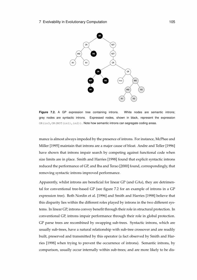
7 Evolvability in Evolutionary Computation 105
NOT
AND
IN2IN1
AND
IN3
OR
TRUE
OR
NOT
IN2
OR
NOT
IN1
IN1
AND
IN1
OR
IN3
OR
Figure 7.2. A GP expression tree containing introns. White nodes are semantic introns;
grey nodes are syntactic introns. Expressed nodes, shown in black, represent the expression
OR(in3,OR(NOT(in1),in2)). Note how semantic introns can segregate coding areas.
mance is almost always impeded by the presence of introns. For instance, McPhee and
Miller [1995] maintain that introns are a major cause of bloat. Andre and Teller [1996]
have shown that introns impair search by competing against functional code when
size limits are in place. Smith and Harries [1998] found that explicit syntactic introns
reduced the performance of GP, and Iba and Terao [2000] found, correspondingly, that
removing syntactic introns improved performance.
Apparently, whilst introns are beneficial for linear GP (and GAs), they are detrimen-
tal for conventional tree-based GP (see figure 7.2 for an example of introns in a GP
expression tree). Both Nordin et al. [1996] and Smith and Harries [1998] believe that
this disparity lies within the different roles played by introns in the two different sys-
tems. In linear GP, introns convey benefit through their role in structural protection. In
conventional GP, introns impair performance through their role in global protection.
GP parse trees are recombined by swapping sub-trees. Syntactic introns, which are
usually sub-trees, have a natural relationship with sub-tree crossover and are readily
built, preserved and transmitted by this operator (a fact observed by Smith and Har-
ries [1998] when trying to prevent the occurrence of introns). Semantic introns, by
comparison, usually occur internally within sub-trees; and are more likely to be dis-
7 Evolvability in Evolutionary Computation 106
rupted rather than constructed by sub-tree crossover. This means that within conven-
tional GP there is a substantial bias towards construction and propagation of syntactic
introns over semantic introns: and therefore a substantial bias towards global pro-
tection over structural protection. In effect, conventional GP suffers from too much
global protection from crossover without gaining any benefits from structural protec-
tion. However, global protection can be reduced by limiting the growth of syntactic
introns. Successful approaches include the removal of introns (the identification of
which can be computationally expensive [Iba and Terao, 2000]) and limiting the be-
haviour of the crossover operator [e.g. Blickle and Thiele, 1994].
7.4.2 Coding Redundancy and Neutrality
A redundant code is one for which there are more possible representations than there
are entities to represent. Accordingly, some entities have more than one representa-
tion. Recently, a number of studies have investigated whether or not redundant codes
can confer an evolutionary advantage over non-redundant codes in the context of ge-
netic algorithms [Shipman, 1999, Shipman et al., 2000, Shackleton et al., 2000, Ebner
et al., 2001, Knowles and Watson, 2002, Rothlauf and Goldberg, 2002, Barreau, 2002].
Work by Shipman et al. [Shipman, 1999, Shipman et al., 2000, Shackleton et al., 2000,
Ebner et al., 2001], in particular, has looked at the role of neutrality during the evolu-
tion of entities represented by redundant codes. This work has made use of a variety of
representations with differing levels of redundancy. These include a direct mapping,
where each solution is represented by exactly one binary string; random mappings,
where each solution is represented by many un-related binary strings; voting map-
pings, where binary solution traits are encoded by more than one bit in the binary
string and where the trait is determined by voting between these bits; and more com-
plex mappings where binary strings describe state machines whose operation deter-
mines the configuration of the solution. Apart from the direct mapping, all of these ex-
hibit a high level of redundancy. However, analysis of the connectivity of their search
spaces (where connections are determined by single point mutations) shows that these
mappings differ considerably in their patterns of neutrality [Shackleton et al., 2000,
Ebner et al., 2001]. Random mappings show very little neutrality, which is to be ex-
pected since there is no logical relationship between different encodings of the same
7 Evolvability in Evolutionary Computation 107
solution. Where there is no epistasis (sharing of bits between building blocks), vot-
ing mappings exhibit no neutrality. Where there is epistasis, voting mappings exhibit
large neutral networks with considerable connectivity between networks. However,
some of the neutral networks are relatively isolated. Of the complex mappings, the
random Boolean network (RBN) mapping (based upon Kauffman’s [1969] model of
gene expression) demonstrates the highest level of neutrality: exhibiting large neutral
networks with very high connectivity between networks. In one configuration, 58%
of mutations are neutral and each encoding has on average 21 non-neutral neighbours
accessible through single point mutations.
In [Ebner et al., 2001], these mappings are applied to a number of optimisation prob-
lems: a random landscape search, a function with many local optima, and a dynamic
fitness function. For all of these problems, performance on mutation-only search cor-
relates with the connectivity of the mappings’ neutral networks. The direct mapping
is unable to solve the first two problems; in part due to insufficient maintenance of
diversity. The non-epistatic voting representation exhibits behaviour which is almost
identical to the direct mapping (an observation which is also made in [Rothlauf and
Goldberg, 2002]). For the redundant mappings, diversity increases over time. These
results have lead the authors to conclude that redundancy can be used to increase the
performance of genetic algorithms: so long as the redundancy is organised in such a
way that leads to neutral networks that percolate the search space.
However, Knowles and Watson [2002] were unable to reproduce these findings when
they compared the performance of direct and RBN mappings upon a variety of more
familiar EC problems. Indeed, aggregated across all the problems they tried, RBN
mappings lead to worse solution times than direct mappings. Nevertheless, they did
find that mappings with high neutrality showed far less sensitivity to mutation rate
than non-redundant mappings. The authors speculate that the slower performance of
RBN mappings may be due to the time overhead involved in random walks across
neutral networks. Whilst these results do not support the conclusions of Ebner et al.,
they do not preclude the possibility that other redundant mappings might be more
effective than the RBN mapping or that neutral networks might be important in solv-
ing larger or more rugged problems than GAs with non-redundant encodings are able
to solve. Further criticism of the redundant mappings used by Shipman et al. can
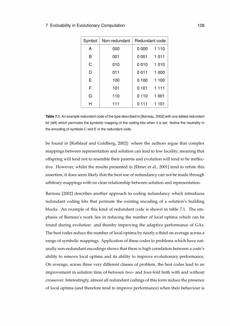
7 Evolvability in Evolutionary Computation 108
Symbol Non-redundant Redundant code
A 000 0 000 1 110
B 001 0 001 1 011
C 010 0 010 1 010
D 011 0 011 1 000
E 100 0 100 1 100
F 101 0 101 1 111
G 110 0 110 1 001
H 111 0 111 1 101
Table 7.1. An example redundant code of the type described in [Barreau, 2002] with one added redundant
bit (left) which permutes the symbolic mapping of the coding bits when it is set. Notice the neutrality in
the encoding of symbols C and E in the redundant code.
be found in [Rothlauf and Goldberg, 2002]: where the authors argue that complex
mappings between representation and solution can lead to low locality; meaning that
offspring will tend not to resemble their parents and evolution will tend to be ineffec-
tive. However, whilst the results presented in [Ebner et al., 2001] tend to refute this
assertion, it does seem likely that the best use of redundancy can not be made through
arbitrary mappings with no clear relationship between solution and representation.
Barreau [2002] describes another approach to coding redundancy which introduces
redundant coding bits that permute the existing encoding of a solution’s building
blocks. An example of this kind of redundant code is shown in table 7.1. The em-
phasis of Barreau’s work lies in reducing the number of local optima which can be
found during evolution: and thereby improving the adaptive performance of GAs.
The best codes reduce the number of local optima by nearly a third on average across a
range of symbolic mappings. Application of these codes to problems which have nat-
urally non-redundant encodings shows that there is high correlation between a code’s
ability to remove local optima and its ability to improve evolutionary performance.
On average, across three very different classes of problem, the best codes lead to an
improvement in solution time of between two- and four-fold both with and without
crossover. Interestingly, almost all redundant codings of this form reduce the presence
of local optima (and therefore tend to improve performance) when their behaviour is
7 Evolvability in Evolutionary Computation 109
averaged across a large number of problem instances. One group of codes in particular
(whose mappings are based around rotation and symmetry) are guaranteed never to
increase the number of local optima on any problem yet exhibit a marginal reduction
in the number of local optima across all problems.
Barreau has also investigated the relationship between the neutrality found within
his class of redundancy codes and their ability to reduce the number of local optima.
However, the relationship is not linear; but rather there is a positive correlation up to a
certain level (about 50% of maximum) after which increased neutrality tends to be as-
sociated with decreased reduction of local optima. The highest levels of neutrality are
found in those codes which offer no or marginal reduction of local optima. Given the
correlation between reduction of local optima and improvement in performance, these
results would tend to support Knowles and Watson’s view that too much redundancy
can lead to reduced performance.
According to the terminology defined in [Rothlauf and Goldberg, 2002], the codes dis-
cussed above all exhibit more or less uniform redundancy: whereby every solution
has roughly the same number of representations. However, it is also possible to de-
fine redundant codes in which certain solutions are over- or under-represented. This,
according to Rothlauf and Goldberg [2002], leads to search biases which then reduce
or increase performance depending upon whether optimal building blocks are over-
or under-represented: and should therefore be taken into account when designing
redundant codes or introducing redundancy to existing codes.
7.4.3 Functional Redundancy
Functional redundancy occurs when a representation contains more functional infor-
mation than is necessary to construct the entity that it represents. However, this extra
functional information may still have significant evolutionary roles: for instance; (i)
it may have been expressed in previous solutions and therefore represents a poten-
tial source of backtracking; (ii) it may be passed on to future solutions where it may
become expressed; (iii) it is still subject to variation and may therefore evolve into
new functionality; and more generally, (iv) it allows a population to maintain genetic
diversity even when solutions have converged; and (v) it enables neutral evolution.
7 Evolvability in Evolutionary Computation 110
In many representations, sources of structural redundancy are also sources of func-
tional redundancy. GP syntactic introns, for instance, consist of code. Whilst this
code’s meaning is currently irrelevant from a behavioural perspective, it still has a
functional meaning and could be involved in any of the evolutionary roles outlined in
the previous paragraph. Haynes [1996] has investigated the evolutionary advantage
of functional redundancy in GP by constructing a problem in which each sub-tree’s
role is independent of its position within a parse tree. Sub-trees are not expressed
in cases where they describe incomplete, invalid, duplicate or subsumed structures.
Haynes found that removing these redundant sub-trees during evolution led to a re-
duction in performance (the opposite effect to that found by Iba and Terao [2000]): and
attributed this to both loss of diversity and loss of protection from crossover. Haynes,
however, was particularly interested in the impact of the loss of ‘protective backup’
caused by the removal of duplicates of expressed structures; and therefore measured
the change in performance caused by duplicating a solution’s expressed sub-trees after
all non-expressed sub-trees had been removed. Haynes found that more duplication
of a solution’s expressed sub-trees (duplicated up to seven times) led to faster solu-
tion times: suggesting that this kind of functional redundancy, at least, is beneficial to
evolution. He also speculated that syntactic introns could be replaced by duplicated
coding regions in non-positionally independent problem domains to achieve the same
effect.
Angeline [1994] suggests that intronic structures like IF FALSE THEN X ELSE Y
represent a form of emergent diploidy and dominance in GP: where sub-tree X corre-
sponds to a recessive trait and sub-tree Y corresponds to a dominant trait. Changing
the condition from FALSE to TRUE would then amount to a dominance shift. The
concepts of diploidy and dominance have gained a lot of interest in the GA commu-
nity [e.g. Goldberg, 1989, Smith and Goldberg, 1992, Dasgupta and McGregor, 1993,
Collingwood et al., 1996, Levenick, 1999, Weicker and Weicker, 2001] as a way of han-
dling non-stationary problems: problems where the search space changes over the
course of time. Goldberg et al. [Goldberg, 1989, Smith and Goldberg, 1992] have de-
veloped a number of diploid representations for GAs. These use two chromosomes
to encode each solution so that for each gene locus one chromosome contains a dom-
inant allele and the other chromosome contains a recessive allele. Only the dominant
allele is expressed in the solution. The most interesting of these is the triallelic scheme:
7 Evolvability in Evolutionary Computation 111
where each allele has a value of either 1, 0, or 10; where 1 is dominant over 0 and 0
is dominant over 10. Mutation effectively has two roles under this scheme: it can
change the value of an allele by changing a 1 into a 0 or vice versa, but it can also
change the dominance of an allele by changing 1 into 10 or vice versa. In [Smith and
Goldberg, 1992], the authors present results that show this diploid representation to
be more effective than a haploid (single chromosome) representation upon a cyclic
non-stationary problem: finding past optima both faster and with higher fidelity. In
their own words: “diploidy embodies a form of temporal memory that is distributed
across the population...this added diversity is more effective than that induced by mu-
tation, because of its sensitivity to function history”. Collingwood et al. [1996] have
investigated the utility of higher levels of polyploidy in GAs for solving a range of
test problems; finding that solutions with up to nine chromosomes can out-perform
haploid representations.
Dasgupta’s structured GA [Dasgupta and McGregor, 1992a,b, 1993] uses a more com-
plex dominance mechanism which uses analogues of regulatory genes to control the
expression of other genes. The structured GA has a tree-like structure where genes
at a higher level control groups of genes at lower levels. Genes at the lowest level,
which may or may not be expressed depending upon the state of higher level genes,
encode components of the solution. Dominance is enforced by limiting the number of
regulatory genes which may be turned on at a given level. Dasgupta believes that the
structured GA is more suitable for non-stationary functions than diploid GAs since
whole blocks of genes may be turned on and off through a single regulatory gene
mutation; and in [Dasgupta and McGregor, 1992b] presents results which show the
structured GA achieving higher performance on the problem described in [Smith and
Goldberg, 1992]. The structured GA also performs well on stationary problems. Re-
sults presented in [Dasgupta and McGregor, 1992a] show that the structured GA per-
forms better than a conventional GA on a difficult engineering optimisation problem.
Dasgupta believes that this is due to the structured GA’s ability to retain greater ge-
netic diversity.
In conventional GP, the level of functional redundancy is determined in part by the
problem domain: since functional redundancy can only occur if the function and ter-
minal sets can be used to construct introns. In cartesian GP, by comparison, functional
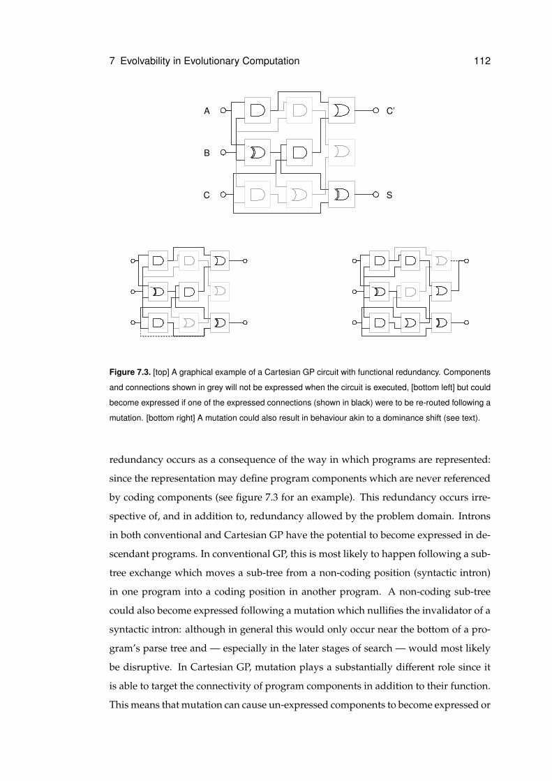
7 Evolvability in Evolutionary Computation 112
A
B
C
C’
S
Figure 7.3. [top] A graphical example of a Cartesian GP circuit with functional redundancy. Components
and connections shown in grey will not be expressed when the circuit is executed, [bottom left] but could
become expressed if one of the expressed connections (shown in black) were to be re-routed following a
mutation. [bottom right] A mutation could also result in behaviour akin to a dominance shift (see text).
redundancy occurs as a consequence of the way in which programs are represented:
since the representation may define program components which are never referenced
by coding components (see figure 7.3 for an example). This redundancy occurs irre-
spective of, and in addition to, redundancy allowed by the problem domain. Introns
in both conventional and Cartesian GP have the potential to become expressed in de-
scendant programs. In conventional GP, this is most likely to happen following a sub-
tree exchange which moves a sub-tree from a non-coding position (syntactic intron)
in one program into a coding position in another program. A non-coding sub-tree
could also become expressed following a mutation which nullifies the invalidator of a
syntactic intron: although in general this would only occur near the bottom of a pro-
gram’s parse tree and — especially in the later stages of search — would most likely
be disruptive. In Cartesian GP, mutation plays a substantially different role since it
is able to target the connectivity of program components in addition to their function.
This means that mutation can cause un-expressed components to become expressed or
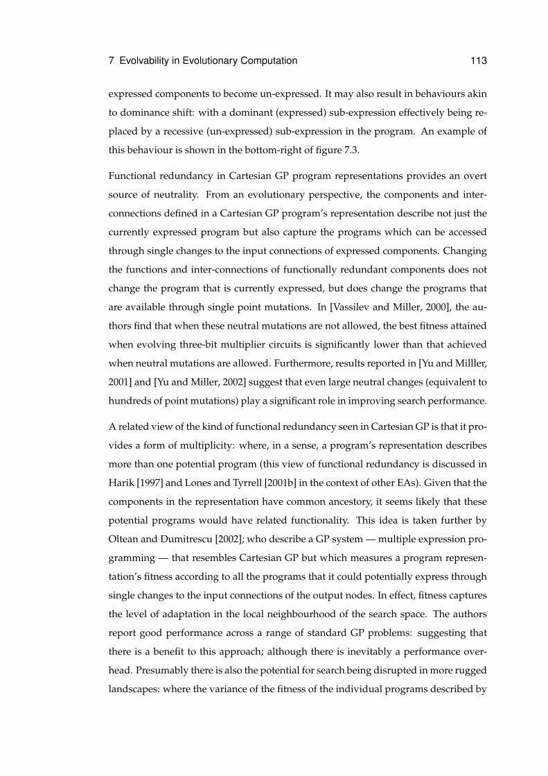
7 Evolvability in Evolutionary Computation 113
expressed components to become un-expressed. It may also result in behaviours akin
to dominance shift: with a dominant (expressed) sub-expression effectively being re-
placed by a recessive (un-expressed) sub-expression in the program. An example of
this behaviour is shown in the bottom-right of figure 7.3.
Functional redundancy in Cartesian GP program representations provides an overt
source of neutrality. From an evolutionary perspective, the components and inter-
connections defined in a Cartesian GP program’s representation describe not just the
currently expressed program but also capture the programs which can be accessed
through single changes to the input connections of expressed components. Changing
the functions and inter-connections of functionally redundant components does not
change the program that is currently expressed, but does change the programs that
are available through single point mutations. In [Vassilev and Miller, 2000], the au-
thors find that when these neutral mutations are not allowed, the best fitness attained
when evolving three-bit multiplier circuits is significantly lower than that achieved
when neutral mutations are allowed. Furthermore, results reported in [Yu and Milller,
2001] and [Yu and Miller, 2002] suggest that even large neutral changes (equivalent to
hundreds of point mutations) play a significant role in improving search performance.
A related view of the kind of functional redundancy seen in Cartesian GP is that it pro-
vides a form of multiplicity: where, in a sense, a program’s representation describes
more than one potential program (this view of functional redundancy is discussed in
Harik [1997] and Lones and Tyrrell [2001b] in the context of other EAs). Given that the
components in the representation have common ancestory, it seems likely that these
potential programs would have related functionality. This idea is taken further by
Oltean and Dumitrescu [2002]; who describe a GP system — multiple expression pro-
gramming — that resembles Cartesian GP but which measures a program represen-
tation’s fitness according to all the programs that it could potentially express through
single changes to the input connections of the output nodes. In effect, fitness captures
the level of adaptation in the local neighbourhood of the search space. The authors
report good performance across a range of standard GP problems: suggesting that
there is a benefit to this approach; although there is inevitably a performance over-
head. Presumably there is also the potential for search being disrupted in more rugged
landscapes: where the variance of the fitness of the individual programs described by
7 Evolvability in Evolutionary Computation 114
a program representation may be high. A recent paper by Hornby [2003] introduces
another approach to encoding multiple solutions within a single representation, using
it to evolve parameterised design families.
7.5 Positional Independence
It is perhaps taken for granted by biologists; but from the perspective of evolution-
ary computation, independence between the behaviour of a gene product and the
position of its gene locus is a significant source of de-constraint within biological rep-
resentations. Within most EC representations the meaning of a genetic component
is determined by its absolute or relative position. This inevitably leads to problems
during recombination. In GAs it may not be possible to find an optimal solution if
components of optimal building blocks are assigned positions that are too far apart in
the solution chromosome. In most forms of GP a component’s context is determined
by its position within the program representation. Given that crossover does not typ-
ically preserve a component’s position, it is quite likely that its context, and therefore
its function, will be lost following recombination. This section discusses existing ap-
proaches to removing positional dependence from EAs.
7.5.1 Linkage Learning
Linkage learning is the GA analogue of epistatic clustering. Linkage learning is mo-
tivated by the desire that all the genetic members of a building block should be in-
herited together during recombination in order to prevent their destruction. Accord-
ing to Smith [2002]: “for a problem composed of a number of separable components,
the genes in the building blocks coding for the component solutions will ideally ex-
hibit high intra-block linkage but low inter-block linkage [to encourage exploration]”.
The simplest approach to linkage learning involves limiting crossover so that it is less
likely or unable to fall between genes whose alleles are considered to belong to the
same building block. This is typically achieved by using crossover templates (success-
ful approaches include those by Rosenberg [1967] and Schaffer and Morishima [1987]),
though it may also be encouraged with explicit introns (see section 7.4.1). However,
these approaches do not target the underlying cause of the linkage problem: positional
7 Evolvability in Evolutionary Computation 115
dependence. Rather, they cause a kind of implicit epistatic clustering which is unlikely
to benefit linked genes located far apart in the solution chromosome. Such a situation
can only be remedied by moving the genes closer together within the chromosome.
However, for most problems the optimal ordering of genes is not known in advance.
Furthermore, it is generally not desirable for a genetic algorithm to rely upon domain
knowledge.
7.5.2 Floating Representations
An obvious solution to this problem is to allow the ordering of genes within a chro-
mosome to evolve. This requires that a gene can occupy any position within the chro-
mosome without losing its original context. Typically this is achieved by associating
each gene allele with some kind of identifier which — in the absence of positional
information — shows the gene locus that it corresponds to. A prominent early exam-
ple of this approach is Bagley’s [1967] inversion operator. However early approaches
such as Bagley’s had little success, primarily due to competition between selection for
fit solutions and selection for fit orderings; not to mention the problem of designing
crossover operators which can appropriately recombine solution chromosomes with
different orderings and the associated problems of under- and over- specification of
gene alleles. Nevertheless, these so-called ‘floating representation’ approaches have
proven successful in domains where under- and over- specification is not an issue
[Raich and Ghaboussi, 1997, Wu and Lindsay, 1996a].
The messy GA [Goldberg et al., 1993] was the first broadly successful approach to
use a floating representation to achieve linkage learning. The messy GA is an iter-
ative algorithm where each iteration consists of a primordial phase: where building
block identification takes place; and a juxtapositional phase: where building blocks
are assembled into complete solutions. During each iteration, the algorithm attempts
to identify and assemble higher level building blocks. Candidate solutions are rep-
resented by variable length chromosomes consisting of < locus, allele > pairs. Each
gene locus may be associated with any number of alleles. Where a locus is associated
with more than one allele, the one which is defined nearest the left of the chromosome
will be used during the solution’s evaluation. If a solution has no alleles defined for
some of its gene loci, values are taken from a template chromosome. The best solution
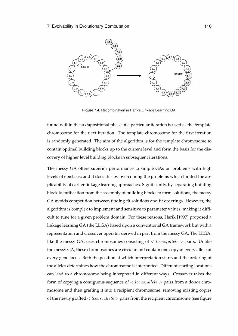
7 Evolvability in Evolutionary Computation 116
5,1
8,0
4,1
2,0
6,0
4,0
2,1
1,1
8,1
3,0
7,0
7,1
5,0
1,0
6,1
3,1
2,1
3,0
7,0
5,1
5,0START
4,1
7,1
8,0
2,0
6,0
4,0
5,1
1,1
8,1
3,1
1,0
6,1
7,0
5,0
2,1
3,0
START
Figure 7.4. Recombination in Harik’s Linkage Learning GA.
found within the juxtapositional phase of a particular iteration is used as the template
chromosome for the next iteration. The template chromosome for the first iteration
is randomly generated. The aim of the algorithm is for the template chromosome to
contain optimal building blocks up to the current level and form the basis for the dis-
covery of higher level building blocks in subsequent iterations.
The messy GA offers superior performance to simple GAs on problems with high
levels of epistasis; and it does this by overcoming the problems which limited the ap-
plicability of earlier linkage learning approaches. Significantly, by separating building
block identification from the assembly of building blocks to form solutions, the messy
GA avoids competition between finding fit solutions and fit orderings. However, the
algorithm is complex to implement and sensitive to parameter values, making it diffi-
cult to tune for a given problem domain. For these reasons, Harik [1997] proposed a
linkage learning GA (the LLGA) based upon a conventional GA framework but with a
representation and crossover operator derived in part from the messy GA. The LLGA,
like the messy GA, uses chromosomes consisting of < locus, allele > pairs. Unlike
the messy GA, these chromosomes are circular and contain one copy of every allele of
every gene locus. Both the position at which interpretation starts and the ordering of
the alleles determines how the chromosome is interpreted. Different starting locations
can lead to a chromosome being interpreted in different ways. Crossover takes the
form of copying a contiguous sequence of < locus, allele > pairs from a donor chro-
mosome and then grafting it into a recipient chromosome, removing existing copies
of the newly grafted < locus, allele > pairs from the recipient chromosome (see figure
7 Evolvability in Evolutionary Computation 117
7.4 for an example). The effect of crossover is to re-arrange the ordering of both alleles
and gene loci within a chromosome: changing both its interpretation and the linkage
between its gene loci. Whilst unlike the messy GA the LLGA does not separate build-
ing block identification from building block assembly, it does avoid the problems with
crossover and under- and over-specification found with earlier approaches and does
avoid the complexities of the messy GA.
Floating representation has also been used within GP; though with limited success. In
a biologically-inspired system described by Luke et al. [1999], a finite state automata
is represented by a sequence of ‘genes’; each of which is identified by a pattern, de-
scribes a state, and declares its connections in terms of the identity patterns of other
genes. During a development process, each state attempts to connect to states whose
patterns most closely match its input patterns. Whilst able to solve a range of string
classification problems, this method shows little improvement over conventional GP.
7.5.3 Gene Expression
An altogether different approach to positional independence can be seen in Wu and
Garibay’s [2002] proportional GA and Ryan et al’s [2002] Chorus GP system; where
both sets of authors have taken inspiration from the role of protein concentration
within gene expression. The proportional GA uses variable-length chromosomes com-
prised of symbols taken from a parameter alphabet; where each symbol corresponds
to a particular parameter. The value of a parameter is determined by the proportion of
its corresponding symbol within a chromosome — in much the same way that certain
phenotypic traits are determined by the concentration, rather than just the presence,
of a particular gene product. The precision with which each parameter is described
depends upon the length of the chromosome: a factor which, the authors believe,
leads to competition between solution length and precision. Across a range of prob-
lems, the proportional GA offers at least as good performance as the simple GA; with
significantly better performance upon certain problems. The authors attribute this im-
provement to the proportional GA’s ability to reduce the size of the search space by
sacrificing unnecessary precision.
Ryan et al’s [2002] Chorus system is based upon grammatical evolution. In GE, the
meaning of a gene is calculated respective to the current grammar transition. In Cho-
7 Evolvability in Evolutionary Computation 118
rus, by comparison, each gene refers to a specific rule within the grammar. As for GE,
a Chorus program is interpreted from left to right. However, a gene only causes a
grammar rule to be fired if it refers to a transition which is currently applicable: and
only if there are no other relevant rules waiting to be expressed. If a gene refers to a
rule which cannot currently be applied, the rule’s entry in a ‘concentration table’ is in-
cremented; showing that it is waiting to be expressed. Accordingly, a particular gene
might have either an immediate or a delayed effect; meaning that its position within
the program is not necessarily indicative of when it will be executed. However, pos-
sibly due to the greater fragility of its representation towards the effects of mutation,
Chorus programs appear not to evolve as well as GE programs [Azad and Ryan, 2003].
7.6 Summary
This chapter has introduced four different approaches to improving the evolvability of
the artefacts which are evolved by evolutionary computation techniques: homologous
recombination, pleiotropy, redundancy, and positional independence. Whilst this re-
view is biased towards techniques which adapt representation rather than those which
adapt variation, it is interesting to note that homologous crossover can lead to an
improvement in evolutionary performance. However, this performance gain is only
significant for linear GP: which has a representation which easily supports homolo-
gous recombination. For conventional tree-based GP, the difficulty of implementing
homologous recombination is reflected by a high computational overhead and little
improvement in performance. By comparison, the introduction of pleiotropy (genetic
re-use) into tree-based genetic programming has proved a very successful approach.
This tends to reflect the biological viewpoint that a degree of pleiotropy helps evolu-
tion by preventing the need to re-evolve identical sub-structures more than once. The
tendency for evolving programs to make use of implicit re-use within graph-based
representations also supports this point of view.
Redundancy plays a range of interesting roles in evolutionary computation. Its capac-
ity to provide structural protection from change has been the subject of a number of
investigations. There appears to be some benefit to introducing structural redundancy
into GA representations, particularly floating representations. Tree-based GP exhibits
7 Evolvability in Evolutionary Computation 119
a high level of natural structural redundancy. However, this redundancy is generated
by syntactic introns which accumulate at the bottom of programs; providing global
protection to change which degrades performance and causes bloat. Nevertheless, re-
sults from linear GP suggest that appropriate forms of non-coding components can
lead to better performance and better solution generality: though unfortunately this
kind of redundancy is inherently unstable within tree-based GP.
Research into coding redundancy in GAs also suggests that performance gains should
only be expected when redundancy is suitably organised. For example, codes which
use redundancy to remove local optima generate a proportional increase in perfor-
mance. However, there is some debate over the utility of neutrality within codes;
though it appears that a degree of neutrality can benefit search by maintaining higher
diversity within a population; although too much neutrality appears to reduce perfor-
mance, possibly by reducing solution locality and introducing extra search overheads.
The functional role of redundancy is particularly interesting, though perhaps least
understood. Functional redundancy plays a particularly important role when solving
non-stationary problems, where it helps to buffer previous solutions. However, it is
also known to improve performance upon stationary problems in both GA and GP:
though again the organisation of redundancy appears to be an important determining
factor. The value of functional redundancy is perhaps best seen within approaches like
multiple expression programming which make explicit use of non-coding components
in evaluating a solution.
From the perspective of evolutionary computation, positional independence in biol-
ogy seems like an important source of evolvability. Linkage learning GAs show how
positional independence can be successfully introduced into EC representations. Po-
sitional independence can also be introduced to GP, but so far only within non-tree
based systems and without any significant increase in performance.
7.7 Perspectives
On the whole, the research reviewed in this chapter supports the notion that biological
concepts can be used within evolutionary computation in order to improve evolvabil-
ity. What is perhaps less clear is that this research also impacts upon our understand-
7 Evolvability in Evolutionary Computation 120
ing of biology, where current understanding of evolvability is mostly at a theoretical
rather than experimental level. For instance, pleiotropy is evidently a powerful source
of evolvability within EC: and this supports the idea that pleiotropy is also important
within biological evolution — and future EC research could give more insight into
what is an appropriate balance between pleiotropy and compartmentalisation. EC re-
search also supports biological theories of the role of non-coding DNA in affirming
structural protection. However, in other regards biological theories of redundancy are
more advanced than EC practice. The role of redundancy structures in supporting
gradual molecular evolution, for instance, could be an interesting inspiration for fu-
ture EC research. Furthermore, future research directions could be measured more by
the topics which are not covered in this chapter rather than those that are. For exam-
ple: multiple weak interactions, exploratory mechanisms, epigenetic inheritance, and
ecological interactions are all thought important in the evolution of biological systems.
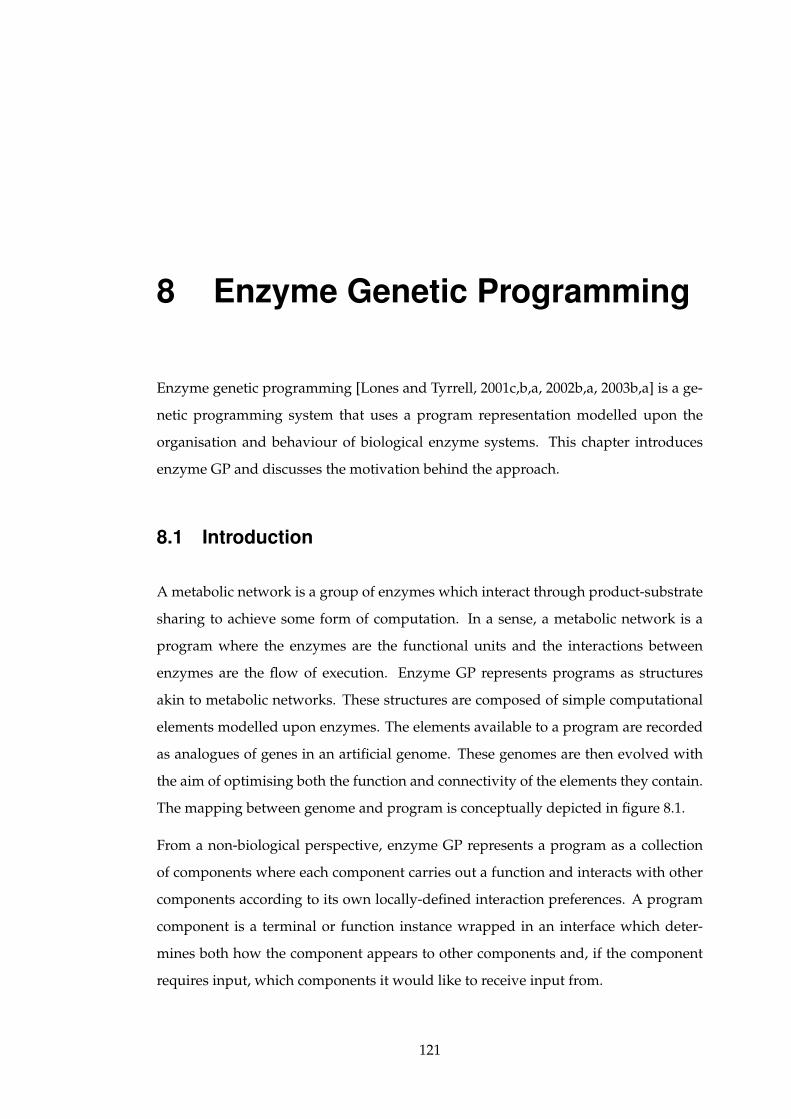
8 Enzyme Genetic Programming
Enzyme genetic programming [Lones and Tyrrell, 2001c,b,a, 2002b,a, 2003b,a] is a ge-
netic programming system that uses a program representation modelled upon the
organisation and behaviour of biological enzyme systems. This chapter introduces
enzyme GP and discusses the motivation behind the approach.
8.1 Introduction
A metabolic network is a group of enzymes which interact through product-substrate
sharing to achieve some form of computation. In a sense, a metabolic network is a
program where the enzymes are the functional units and the interactions between
enzymes are the flow of execution. Enzyme GP represents programs as structures
akin to metabolic networks. These structures are composed of simple computational
elements modelled upon enzymes. The elements available to a program are recorded
as analogues of genes in an artificial genome. These genomes are then evolved with
the aim of optimising both the function and connectivity of the elements they contain.
The mapping between genome and program is conceptually depicted in figure 8.1.
From a non-biological perspective, enzyme GP represents a program as a collection
of components where each component carries out a function and interacts with other
components according to its own locally-defined interaction preferences. A program
component is a terminal or function instance wrapped in an interface which deter-
mines both how the component appears to other components and, if the component
requires input, which components it would like to receive input from.
121
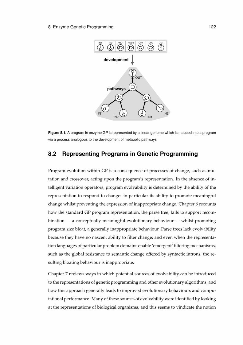
8 Enzyme Genetic Programming 122
IN2IN1 AND1 AND2 OR1 OR2 OUT
IN2 IN1
OUT
IN1 IN2
pathways
development
Figure 8.1. A program in enzyme GP is represented by a linear genome which is mapped into a program
via a process analogous to the development of metabolic pathways.
8.2 Representing Programs in Genetic Programming
Program evolution within GP is a consequence of processes of change, such as mu-
tation and crossover, acting upon the program’s representation. In the absence of in-
telligent variation operators, program evolvability is determined by the ability of the
representation to respond to change: in particular its ability to promote meaningful
change whilst preventing the expression of inappropriate change. Chapter 6 recounts
how the standard GP program representation, the parse tree, fails to support recom-
bination — a conceptually meaningful evolutionary behaviour — whilst promoting
program size bloat, a generally inappropriate behaviour. Parse trees lack evolvability
because they have no nascent ability to filter change; and even when the representa-
tion languages of particular problem domains enable ‘emergent’ filtering mechanisms,
such as the global resistance to semantic change offered by syntactic introns, the re-
sulting bloating behaviour is inappropriate.
Chapter 7 reviews ways in which potential sources of evolvability can be introduced
to the representations of genetic programming and other evolutionary algorithms, and
how this approach generally leads to improved evolutionary behaviours and compu-
tational performance. Many of these sources of evolvability were identified by looking
at the representations of biological organisms, and this seems to vindicate the notion
8 Enzyme Genetic Programming 123
that biological modelling can be used to improve the behaviour and performance of
evolutionary computation — and forms part of the motivation for the development
of enzyme genetic programming. The program representation used by enzyme GP is
modelled both upon the way in which the function of biochemical pathways emerges
from the sum of the behaviours of individual proteins and enzymes, and upon the way
in which these systems respond to genetic change. Enzyme GP possesses many of the
characteristics identified within the previous chapter as being sources of evolvability:
including positional independence, functional and structural redundancy, neutrality,
and implicit reuse.
The role of context within program representation is perhaps central to an understand-
ing of enzyme GP and how it differs from other genetic programming approaches.
According to the definition given in Section 6.3, a program component’s context is de-
termined by where it receives its inputs from: since this determines the arguments to
which its function will be applied and therefore its outputs and hence its role within
the program.
8.2.1 Explicit context
Within a parse tree, the context of a program component is determined by its posi-
tion within the structure. For the remainder of this manuscript, this form of context is
called explicit context, reflecting the fact that a component’s context is recorded explic-
itly by its position within the representation relative to other components. Other GP
approaches which use explicit context representations include linear GP [e.g. Nordin,
1994] and grammatical evolution [e.g. Ryan et al., 1998]. Explicit context represen-
tations have two properties which limit their ability to be evolved. The first, that a
component’s context is determined by position, that crossover operators do not pre-
serve this position, and that therefore contextual information is easily lost, has already
been discussed at length. Second, explicit context usually enforces a one-to-one map-
ping between representation and program, such that changes to the representation
lead directly to changes within the program. The variation operators therefore act di-
rectly upon the program, implying that evolution is determined solely by processes
of variation and selection. The representation, by comparison, has no dynamic role to
play within the evolutionary process.
8 Enzyme Genetic Programming 124
A
B
C
C’
S
A
B
C
C’
S
A
B
C
C’
S
Figure 8.2. Recombination can cause loss of context when indirect context is used. A cartesian GP
circuit is recombined with a flipped version of itself, but due to the same components occupying different
locations in the two circuits, context (and consequently behaviour) is not preserved in the recombined
circuit. Recombined parts are shaded grey.
8.2.2 Indirect context
In some other GP representations [e.g. Poli, 1997, Miller and Thomson, 2000], con-
nections between components are specified using indirection. Typically each compo-
nent is assigned a reference (which may be a location, a number or an arbitrary code)
and other components specify their input connections using these references. A good
example of this is Cartesian GP [Miller and Thomson, 2000], where components are
assigned to locations in a cartesian co-ordinate system and input connections are ex-
pressed in terms of the co-ordinates of components they wish to receive inputs from.
Context within these representations is specified indirectly, hence this form of context
is termed indirect context.
Indirect context representations support a number of interesting evolutionary behav-
iours. Perhaps most significantly, a component only becomes active in a program
if another component expresses a connection to it. Otherwise it is recessive. This
has some important implications. If a new component is added to the representation
8 Enzyme Genetic Programming 125
during recombination, it will only become active in the program if its reference is
addressed by an existing component or it is an output node. This effect is termed
variation filtering, since the representation only expresses certain variation events in
the program whilst filtering out others.
Indirect context representations usually assign references arbitrarily: such that there
is no correlation between component reference and component behaviour. Indirect
context, therefore, does not declare any behavioural information. Consequently, it
expresses no real meaning other than the connectivity of the current program. This
leads to similar problems to those seen with explicit context representations. Most
significantly, indirect context has no meaning between different programs since com-
ponents with different behaviours can have the same reference and components with
the same behaviour can have different references in different programs. This implies
that recombination is unlikely to preserve context (see figure 8.2). Furthermore, if a
component’s input connection is mutated, there will be no correlation between the de-
gree of mutation and the degree of change to the component’s input context: meaning
that the component’s context cannot be varied gradually, unless by accident.
However, it is conceivable that the population might be able to evolve a correlation
between component reference and component behaviour over the course of time, es-
pecially as the population becomes more homogenous. In this sense, the meaning of
indirect context is evolvable. Furthermore, indirect context representations support
both structural and functional modes of redundancy in addition to a capacity for im-
plicit reuse.
8.3 Implicit Context Representation
By comparison to the explicit and indirect contexts used by GP, biology expresses com-
ponent interactions with what could be called implicit context. With implicit context,
a component’s context is declared implicitly within the component’s definition rather
than being imposed by external factors such as its relative position within a represen-
tation. For example, the behaviour of a bio-chemical is dependent upon its physical
shape and chemical properties. Enzymes, which conceptually receive their input in
the form of bio-chemicals, express their preference for these inputs by the shape and
8 Enzyme Genetic Programming 126
chemical properties of their binding sites. Since the bio-chemicals that they bind have
physical shape and chemical properties complementary to the binding sites, these
binding sites are implicitly describing the enzyme’s context in terms of the behaviour
of the substrates they expect to bind.
8.3.1 An Illustrative Example
Figure 8.3 illustrates an example of an abstract system whose behaviour and evolution
is determined by implicit context. The system is represented by three components:
each of which has a shape, which identifies it to other components; and an implicit
context, which declares the shape of the component it would prefer to interact with.
If the system is allowed to develop, interactions occur according to the implicit con-
texts declared by each component; whereby each component attempts to interact with
a component whose shape most closely matches its own implicit context. In essence,
the system self-organises according to the properties of the components from which
it is comprised. Because of this property of self-organisation, there is no external re-
quirement for a component to be expressed in the developed system. In the example,
a component is added to the representation which does not match any of the implicit
contexts defined by the existing components and is consequently not ‘expressed’ in
the developed structure of the system. Conversely, if a component is added to the
representation which has a better match with one of the existing implicit contexts of
the system, then it does become expressed in the system.
This is another example of a variation filtering process of the kind seen where an
indirect context representation is used. In an indirect context representation, the lack
of correlation between indirect context and behaviour causes variation filtering to be
an arbitrary process. In an implicit context representation, by comparison, variation
filtering is a process which filters out change which does not fit into the current system
context whilst promoting change which improves the internal cohesion of the system.
From an evolutionary perspective, this would seem like a useful function since it tends
to preserve the existing evolved behaviour of the system by lessening the impact of
change and without actually preventing change to the representation.
The bottom two panes in figure 8.3 show the benefits of recessive components within
an implicit context representation. In the first of these, a component which was added
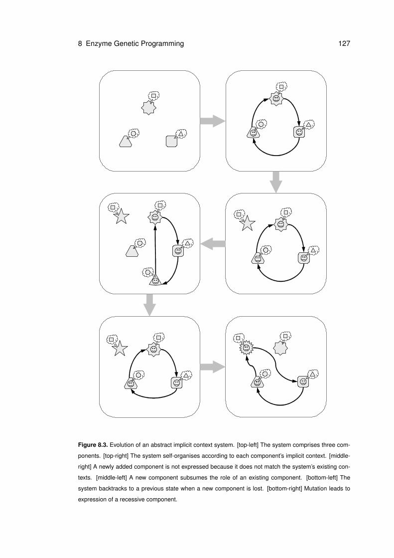
8 Enzyme Genetic Programming 127
Figure 8.3. Evolution of an abstract implicit context system. [top-left] The system comprises three com-
ponents. [top-right] The system self-organises according to each component’s implicit context. [middle-
right] A newly added component is not expressed because it does not match the system’s existing con-
texts. [middle-left] A new component subsumes the role of an existing component. [bottom-left] The
system backtracks to a previous state when a new component is lost. [bottom-right] Mutation leads to
expression of a recessive component.
8 Enzyme Genetic Programming 128
to the system has now been lost; but because the added component had only sub-
sumed the role of an earlier component, rather than replacing it, the earlier compo-
nent is able to resume its role. This demonstrates a capacity for backtracking, showing
how functional redundancy can reduce the impact of the loss of a component upon
the behaviour of the system. In fact, this is another example of variation filtering, but
filtering the effect of removing a component rather than the effect of adding a com-
ponent. The final pane of figure 8.3 shows that recessive components are also able to
undergo evolution. In this case, the mutation of a recessive component allows it to fit
into the context of the system and become expressed.
8.3.2 Representing Programs with Implicit Context
Implicit context does not seem like an obvious approach to representing programs, yet
its pervasiveness in biology and the behaviours described above suggest that it is a
good way of representing an evolving system. Indeed, implicit context representation
seems to fulfill at least the first of Kirschner and Gerhart’s principles of evolvability:
the capacity to reduce the potential lethality of mutations — which it achieves through
the variation filtering process described above, making it less likely that change to a
representation will result in substantial change to the entity that it represents. This in
turn makes it more likely that Kirschner and Gerhart’s second principle will be met: a
capacity to reduce the number of mutations needed to produce phenotypically novel
traits; since there is more chance of the entity surviving a series of changes. Moreover,
the presence of functional redundancy brings with it the potential modes of evolution
described in sections 5.2.1 and 7.4.3; each of which tend to increase the explorative
potential of evolution and hence the likelihood of a series of changes leading to an
improved entity.
It is hoped that implicit context can be used to introduce variation filtering to pro-
gram representations, leading to an improvement in the behaviour and success rate
of conventional GP variation operators, and in particular enabling meaningful recom-
bination. However, there are certain pre-conditions for implicit context to be able to
enable useful variation filtering. These were originally identified in Lones and Tyrrell
[2002a] and concern the relationship between implied context (the context declared in
the representation) and actual context (the context which occurs in the program). Pre-
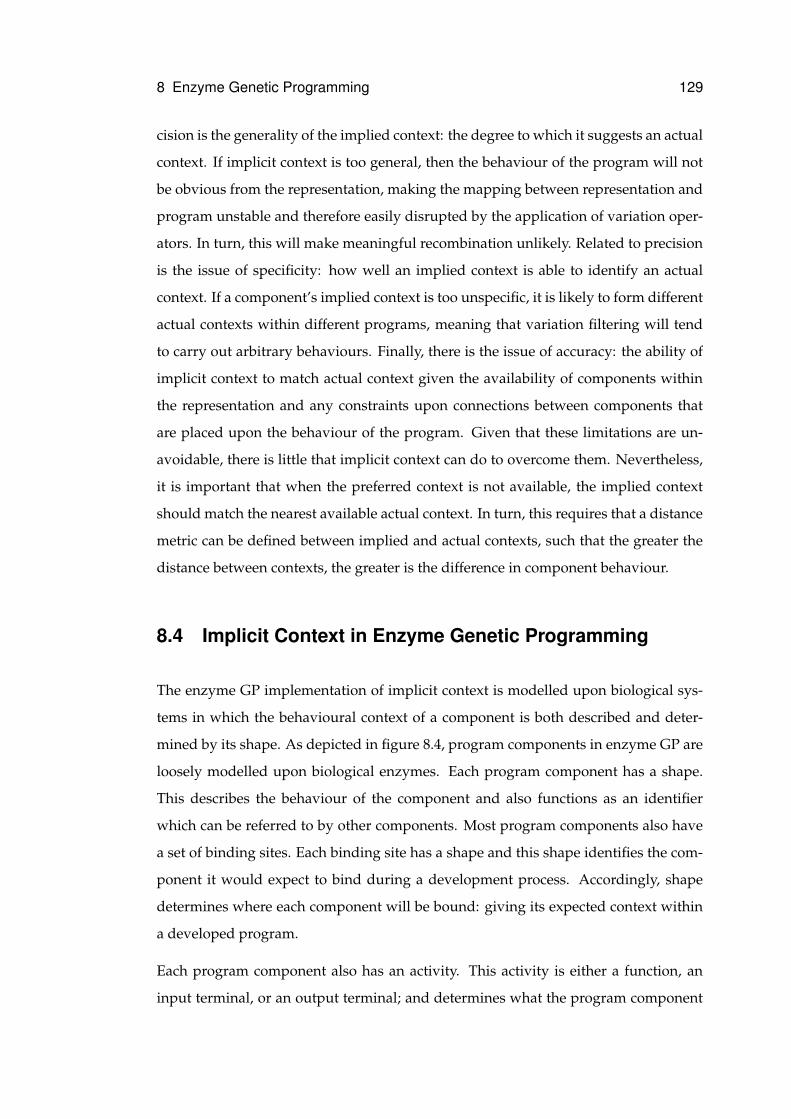
8 Enzyme Genetic Programming 129
cision is the generality of the implied context: the degree to which it suggests an actual
context. If implicit context is too general, then the behaviour of the program will not
be obvious from the representation, making the mapping between representation and
program unstable and therefore easily disrupted by the application of variation oper-
ators. In turn, this will make meaningful recombination unlikely. Related to precision
is the issue of specificity: how well an implied context is able to identify an actual
context. If a component’s implied context is too unspecific, it is likely to form different
actual contexts within different programs, meaning that variation filtering will tend
to carry out arbitrary behaviours. Finally, there is the issue of accuracy: the ability of
implicit context to match actual context given the availability of components within
the representation and any constraints upon connections between components that
are placed upon the behaviour of the program. Given that these limitations are un-
avoidable, there is little that implicit context can do to overcome them. Nevertheless,
it is important that when the preferred context is not available, the implied context
should match the nearest available actual context. In turn, this requires that a distance
metric can be defined between implied and actual contexts, such that the greater the
distance between contexts, the greater is the difference in component behaviour.
8.4 Implicit Context in Enzyme Genetic Programming
The enzyme GP implementation of implicit context is modelled upon biological sys-
tems in which the behavioural context of a component is both described and deter-
mined by its shape. As depicted in figure 8.4, program components in enzyme GP are
loosely modelled upon biological enzymes. Each program component has a shape.
This describes the behaviour of the component and also functions as an identifier
which can be referred to by other components. Most program components also have
a set of binding sites. Each binding site has a shape and this shape identifies the com-
ponent it would expect to bind during a development process. Accordingly, shape
determines where each component will be bound: giving its expected context within
a developed program.
Each program component also has an activity. This activity is either a function, an
input terminal, or an output terminal; and determines what the program component

8 Enzyme Genetic Programming 130
IN2IN1 AND1 AND2 OR1 OR2 OUT
binding sites
activity
shape
ideal substrates
Figure 8.4. Enzyme model. A program component consists of a shape, an activity and a set of binding
sites. Shape describes how the enzyme is seen by other program components. The shape of a binding
site determines which component (or ‘substrate’) will be bound at a particular input.
will do within a developed program. Only components with functional and output
terminal activities have binding sites. Following development, the function or out-
put terminal’s input(s) will be provided by the output of the components which are
bound to the binding sites. Input terminal components provide program inputs at
their outputs.
8.4.1 Functionality
A shape is not just an identifier. Shape also describes the behaviour of a program com-
ponent. It would be insufficient for shape to merely express the activity of a program
component since there will in general be many instances of only a few different func-
tions and terminals within each program. Nevertheless, each of these instances will
be carrying out a different role within each program. The aim of shape within enzyme
GP is to capture this role.
The role of a program component depends not only upon itself and the activity it
carries out but also upon the components it interacts with and the activities they carry
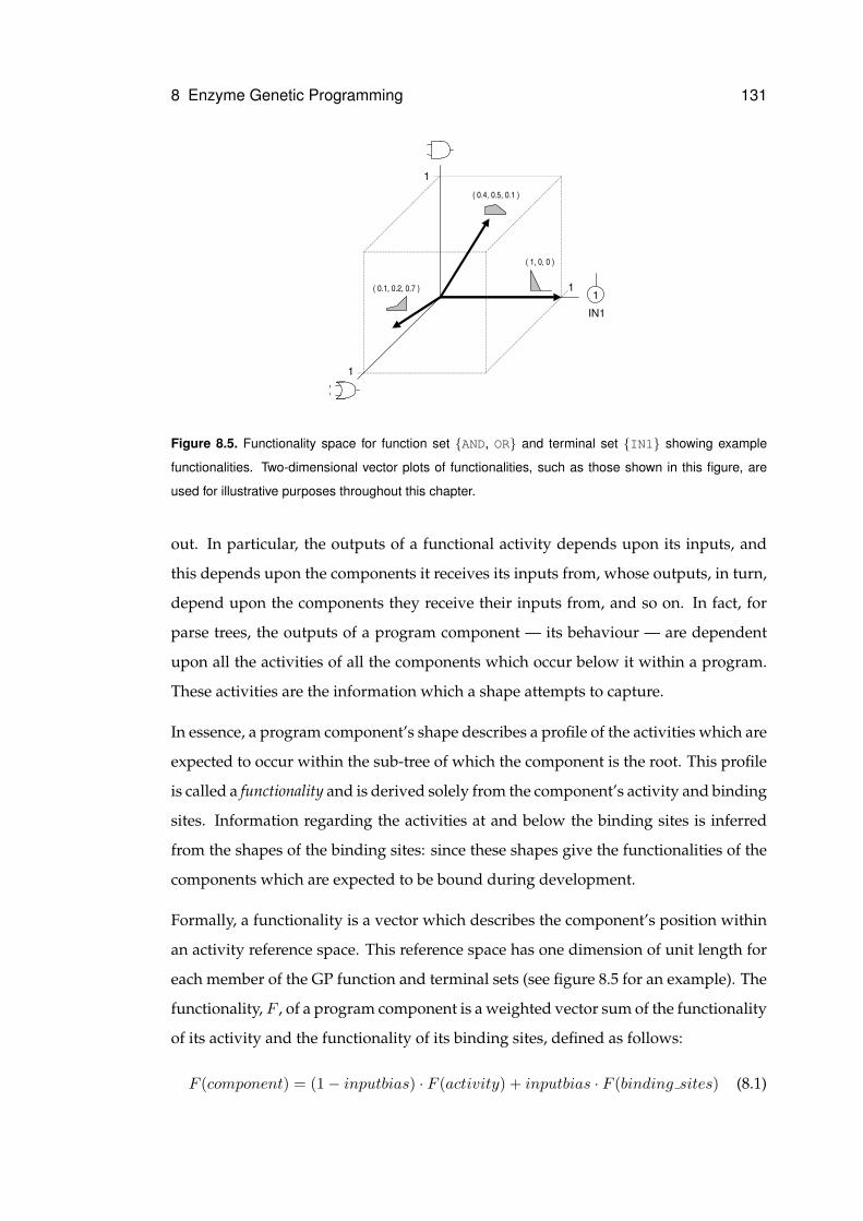
8 Enzyme Genetic Programming 131
IN1
(�0.1,�0.2,�0.7�)
(�0.4,�0.5,�0.1�)
(�1,�0,�0�)
1
1
1
1
Figure 8.5. Functionality space for function set {AND, OR} and terminal set {IN1} showing example
functionalities. Two-dimensional vector plots of functionalities, such as those shown in this figure, are
used for illustrative purposes throughout this chapter.
out. In particular, the outputs of a functional activity depends upon its inputs, and
this depends upon the components it receives its inputs from, whose outputs, in turn,
depend upon the components they receive their inputs from, and so on. In fact, for
parse trees, the outputs of a program component — its behaviour — are dependent
upon all the activities of all the components which occur below it within a program.
These activities are the information which a shape attempts to capture.
In essence, a program component’s shape describes a profile of the activities which are
expected to occur within the sub-tree of which the component is the root. This profile
is called a functionality and is derived solely from the component’s activity and binding
sites. Information regarding the activities at and below the binding sites is inferred
from the shapes of the binding sites: since these shapes give the functionalities of the
components which are expected to be bound during development.
Formally, a functionality is a vector which describes the component’s position within
an activity reference space. This reference space has one dimension of unit length for
each member of the GP function and terminal sets (see figure 8.5 for an example). The
functionality, F , of a program component is a weighted vector sum of the functionality
of its activity and the functionality of its binding sites, defined as follows:
F (component) = (1 − inputbias) · F (activity) + inputbias · F (binding sites) (8.1)
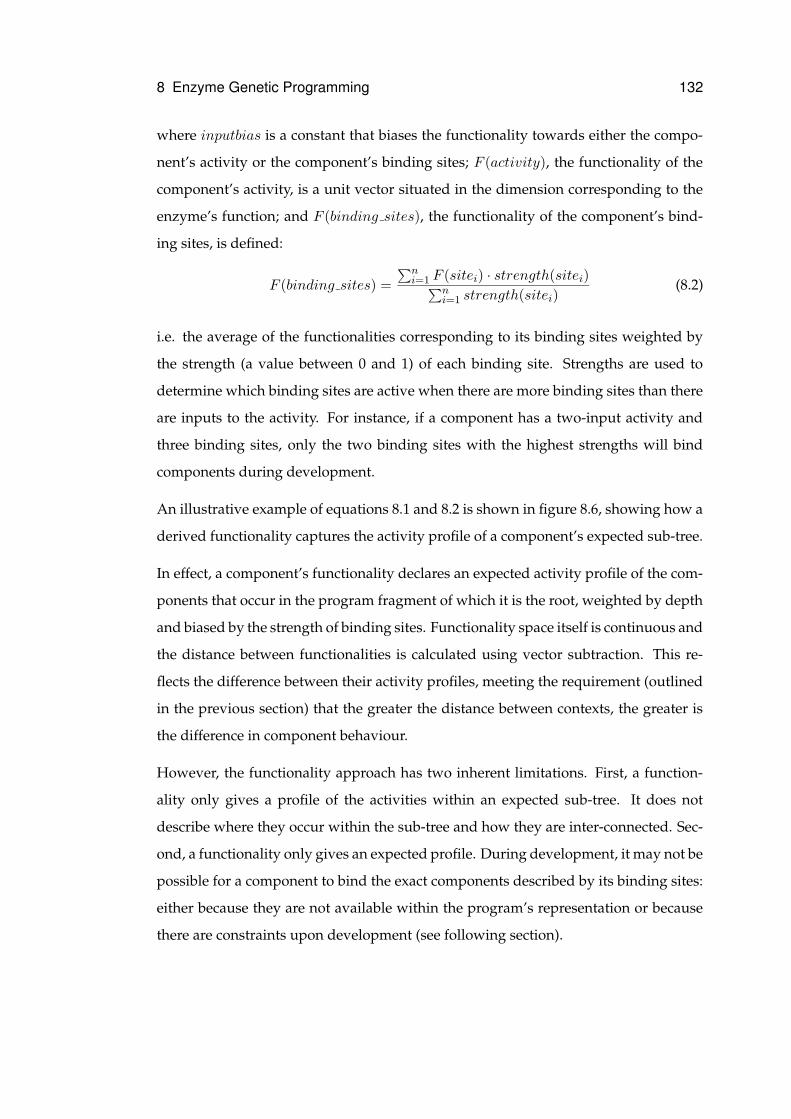
8 Enzyme Genetic Programming 132
where inputbias is a constant that biases the functionality towards either the compo-
nent’s activity or the component’s binding sites; F (activity), the functionality of the
component’s activity, is a unit vector situated in the dimension corresponding to the
enzyme’s function; and F (binding sites), the functionality of the component’s bind-
ing sites, is defined:
F (binding sites) =
∑n
i=1F (sitei) · strength(sitei)
∑n
i=1strength(sitei)
(8.2)
i.e. the average of the functionalities corresponding to its binding sites weighted by
the strength (a value between 0 and 1) of each binding site. Strengths are used to
determine which binding sites are active when there are more binding sites than there
are inputs to the activity. For instance, if a component has a two-input activity and
three binding sites, only the two binding sites with the highest strengths will bind
components during development.
An illustrative example of equations 8.1 and 8.2 is shown in figure 8.6, showing how a
derived functionality captures the activity profile of a component’s expected sub-tree.
In effect, a component’s functionality declares an expected activity profile of the com-
ponents that occur in the program fragment of which it is the root, weighted by depth
and biased by the strength of binding sites. Functionality space itself is continuous and
the distance between functionalities is calculated using vector subtraction. This re-
flects the difference between their activity profiles, meeting the requirement (outlined
in the previous section) that the greater the distance between contexts, the greater is
the difference in component behaviour.
However, the functionality approach has two inherent limitations. First, a function-
ality only gives a profile of the activities within an expected sub-tree. It does not
describe where they occur within the sub-tree and how they are inter-connected. Sec-
ond, a functionality only gives an expected profile. During development, it may not be
possible for a component to bind the exact components described by its binding sites:
either because they are not available within the program’s representation or because
there are constraints upon development (see following section).
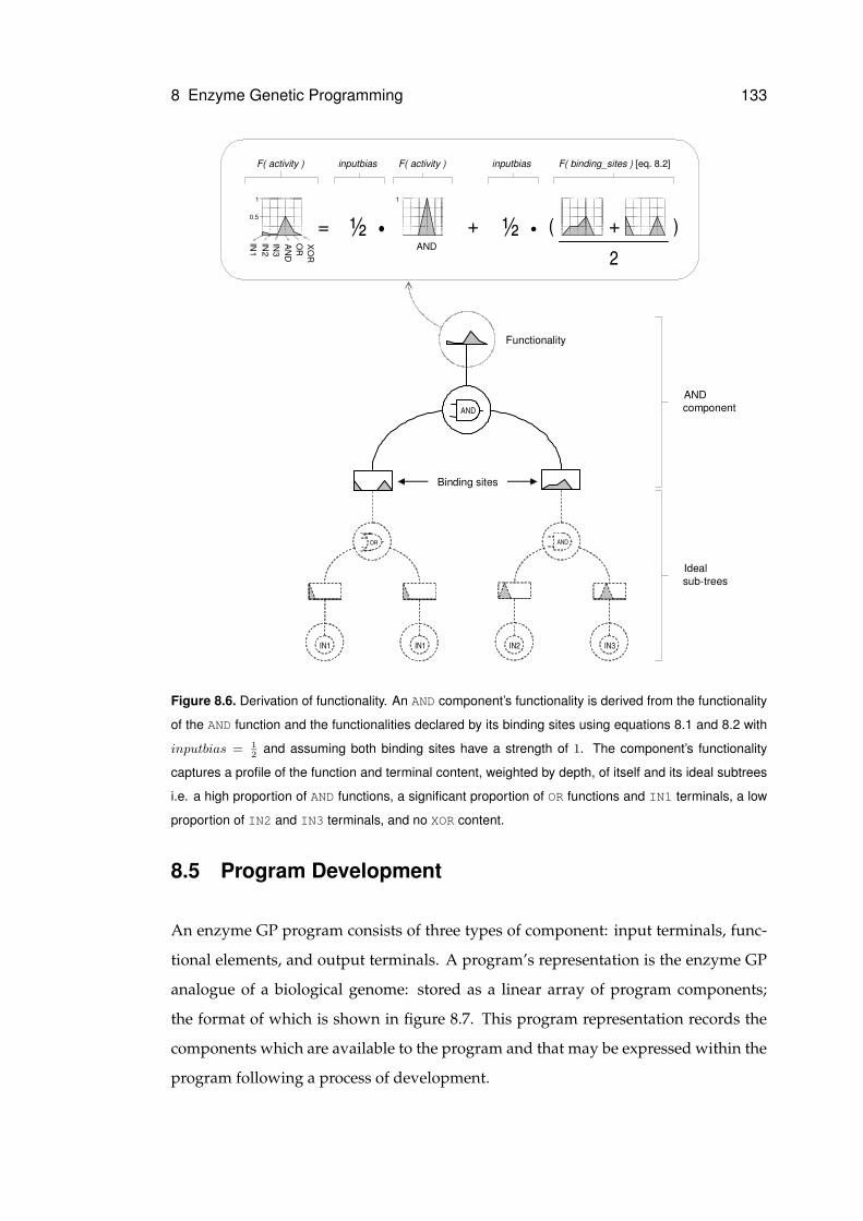
8 Enzyme Genetic Programming 133
IN1
IN1
IN2
AN
DO
RX
OR
IN3
½ •= + ( + )½ •0.5
1
2AND
1
F( activity ) F( binding_sites ) [eq. 8.2]inputbias inputbiasF( activity )
AND
OR AND
IN1 IN2 IN3
Idealsub-trees
Binding sites
Functionality
ANDcomponent
Figure 8.6. Derivation of functionality. An AND component’s functionality is derived from the functionality
of the AND function and the functionalities declared by its binding sites using equations 8.1 and 8.2 with
inputbias = 1
2and assuming both binding sites have a strength of 1. The component’s functionality
captures a profile of the function and terminal content, weighted by depth, of itself and its ideal subtrees
i.e. a high proportion of AND functions, a significant proportion of OR functions and IN1 terminals, a low
proportion of IN2 and IN3 terminals, and no XOR content.
8.5 Program Development
An enzyme GP program consists of three types of component: input terminals, func-
tional elements, and output terminals. A program’s representation is the enzyme GP
analogue of a biological genome: stored as a linear array of program components;
the format of which is shown in figure 8.7. This program representation records the
components which are available to the program and that may be expressed within the
program following a process of development.
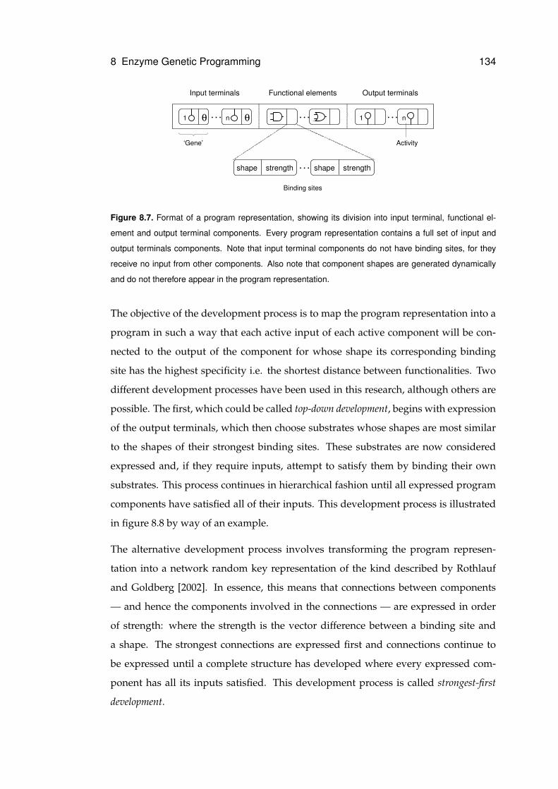
8 Enzyme Genetic Programming 134
… …1 n …1 n
shape strength … shape strength
θ θ
Input terminals Functional elements Output terminals
‘Gene’ Activity
Binding sites
Figure 8.7. Format of a program representation, showing its division into input terminal, functional el-
ement and output terminal components. Every program representation contains a full set of input and
output terminals components. Note that input terminal components do not have binding sites, for they
receive no input from other components. Also note that component shapes are generated dynamically
and do not therefore appear in the program representation.
The objective of the development process is to map the program representation into a
program in such a way that each active input of each active component will be con-
nected to the output of the component for whose shape its corresponding binding
site has the highest specificity i.e. the shortest distance between functionalities. Two
different development processes have been used in this research, although others are
possible. The first, which could be called top-down development, begins with expression
of the output terminals, which then choose substrates whose shapes are most similar
to the shapes of their strongest binding sites. These substrates are now considered
expressed and, if they require inputs, attempt to satisfy them by binding their own
substrates. This process continues in hierarchical fashion until all expressed program
components have satisfied all of their inputs. This development process is illustrated
in figure 8.8 by way of an example.
The alternative development process involves transforming the program represen-
tation into a network random key representation of the kind described by Rothlauf
and Goldberg [2002]. In essence, this means that connections between components
— and hence the components involved in the connections — are expressed in order
of strength: where the strength is the vector difference between a binding site and
a shape. The strongest connections are expressed first and connections continue to
be expressed until a complete structure has developed where every expressed com-
ponent has all its inputs satisfied. This development process is called strongest-first
development.
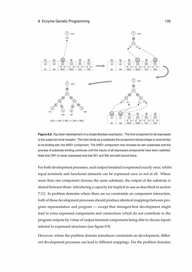
8 Enzyme Genetic Programming 135
OUT
IN2IN1 AND1 AND2 OR1 OR2
OUT
IN2IN1 AND1 AND2 OR1 OR2
OUTOUT
IN2IN1 AND1 AND2 OR1 OR2
IN1 IN2
IN2 IN1
OUT�=�(�IN1�∨ IN2�)�∧ (�IN1�∧ IN2�)�
Figure 8.8. Top-down development of a simple Boolean expression. The first component to be expressed
is the output terminal receptor. This then binds as a substrate the component whose shape is most similar
to its binding site; the AND1 component. The AND1 component now chooses its own substrates and the
process of substrate binding continues until the inputs of all expressed components have been satisfied.
Note that OR1 is never expressed and that IN1 and IN2 are both bound twice.
For both development processes, each output terminal is expressed exactly once, whilst
input terminals and functional elements can be expressed once or not at all. Where
more than one component chooses the same substrate, the output of the substrate is
shared between them: introducing a capacity for implicit re-use as described in section
7.3.2. In problem domains where there are no constraints on component interaction,
both of these development processes should produce identical mappings between pro-
gram representation and program — except that strongest-first development might
lead to extra expressed components and connections which do not contribute to the
program outputs by virtue of output terminal components being able to choose inputs
internal to expressed structures (see figure 8.9).
However, where the problem domain introduces constraints on development, differ-
ent development processes can lead to different mappings. For the problem domains
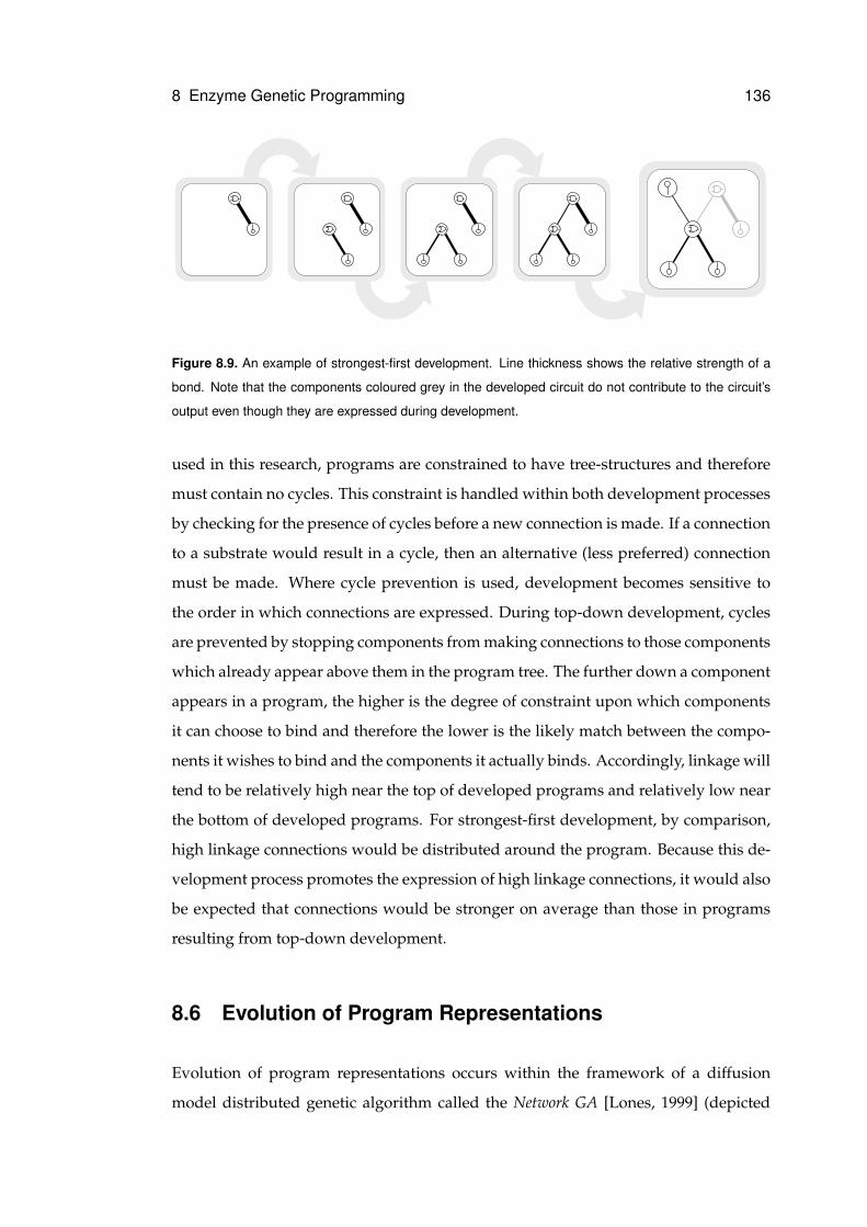
8 Enzyme Genetic Programming 136
Figure 8.9. An example of strongest-first development. Line thickness shows the relative strength of a
bond. Note that the components coloured grey in the developed circuit do not contribute to the circuit’s
output even though they are expressed during development.
used in this research, programs are constrained to have tree-structures and therefore
must contain no cycles. This constraint is handled within both development processes
by checking for the presence of cycles before a new connection is made. If a connection
to a substrate would result in a cycle, then an alternative (less preferred) connection
must be made. Where cycle prevention is used, development becomes sensitive to
the order in which connections are expressed. During top-down development, cycles
are prevented by stopping components from making connections to those components
which already appear above them in the program tree. The further down a component
appears in a program, the higher is the degree of constraint upon which components
it can choose to bind and therefore the lower is the likely match between the compo-
nents it wishes to bind and the components it actually binds. Accordingly, linkage will
tend to be relatively high near the top of developed programs and relatively low near
the bottom of developed programs. For strongest-first development, by comparison,
high linkage connections would be distributed around the program. Because this de-
velopment process promotes the expression of high linkage connections, it would also
be expected that connections would be stronger on average than those in programs
resulting from top-down development.
8.6 Evolution of Program Representations
Evolution of program representations occurs within the framework of a diffusion
model distributed genetic algorithm called the Network GA [Lones, 1999] (depicted
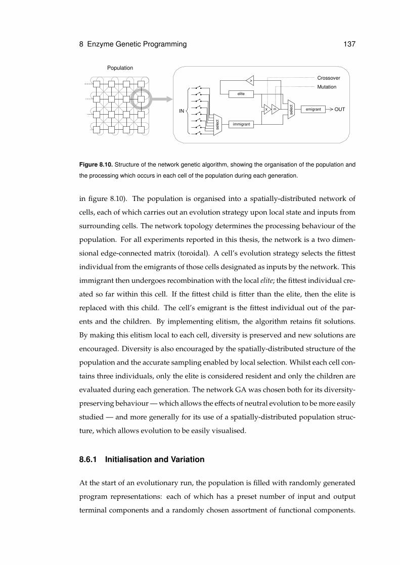
8 Enzyme Genetic Programming 137
Population
elite
sele
ct
immigrant
X m
sele
ct
>
IN emigrant OUT
Crossover
Mutation
Figure 8.10. Structure of the network genetic algorithm, showing the organisation of the population and
the processing which occurs in each cell of the population during each generation.
in figure 8.10). The population is organised into a spatially-distributed network of
cells, each of which carries out an evolution strategy upon local state and inputs from
surrounding cells. The network topology determines the processing behaviour of the
population. For all experiments reported in this thesis, the network is a two dimen-
sional edge-connected matrix (toroidal). A cell’s evolution strategy selects the fittest
individual from the emigrants of those cells designated as inputs by the network. This
immigrant then undergoes recombination with the local elite; the fittest individual cre-
ated so far within this cell. If the fittest child is fitter than the elite, then the elite is
replaced with this child. The cell’s emigrant is the fittest individual out of the par-
ents and the children. By implementing elitism, the algorithm retains fit solutions.
By making this elitism local to each cell, diversity is preserved and new solutions are
encouraged. Diversity is also encouraged by the spatially-distributed structure of the
population and the accurate sampling enabled by local selection. Whilst each cell con-
tains three individuals, only the elite is considered resident and only the children are
evaluated during each generation. The network GA was chosen both for its diversity-
preserving behaviour — which allows the effects of neutral evolution to be more easily
studied — and more generally for its use of a spatially-distributed population struc-
ture, which allows evolution to be easily visualised.
8.6.1 Initialisation and Variation
At the start of an evolutionary run, the population is filled with randomly generated
program representations: each of which has a preset number of input and output
terminal components and a randomly chosen assortment of functional components.
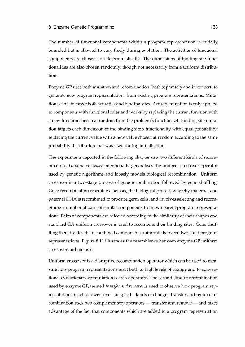
8 Enzyme Genetic Programming 138
The number of functional components within a program representation is initially
bounded but is allowed to vary freely during evolution. The activities of functional
components are chosen non-deterministically. The dimensions of binding site func-
tionalities are also chosen randomly, though not necessarily from a uniform distribu-
tion.
Enzyme GP uses both mutation and recombination (both separately and in concert) to
generate new program representations from existing program representations. Muta-
tion is able to target both activities and binding sites. Activity mutation is only applied
to components with functional roles and works by replacing the current function with
a new function chosen at random from the problem’s function set. Binding site muta-
tion targets each dimension of the binding site’s functionality with equal probability;
replacing the current value with a new value chosen at random according to the same
probability distribution that was used during initialisation.
The experiments reported in the following chapter use two different kinds of recom-
bination. Uniform crossover intentionally generalises the uniform crossover operator
used by genetic algorithms and loosely models biological recombination. Uniform
crossover is a two-stage process of gene recombination followed by gene shuffling.
Gene recombination resembles meiosis, the biological process whereby maternal and
paternal DNA is recombined to produce germ cells, and involves selecting and recom-
bining a number of pairs of similar components from two parent program representa-
tions. Pairs of components are selected according to the similarity of their shapes and
standard GA uniform crossover is used to recombine their binding sites. Gene shuf-
fling then divides the recombined components uniformly between two child program
representations. Figure 8.11 illustrates the resemblance between enzyme GP uniform
crossover and meiosis.
Uniform crossover is a disruptive recombination operator which can be used to mea-
sure how program representations react both to high levels of change and to conven-
tional evolutionary computation search operators. The second kind of recombination
used by enzyme GP, termed transfer and remove, is used to observe how program rep-
resentations react to lower levels of specific kinds of change. Transfer and remove re-
combination uses two complementary operators — transfer and remove — and takes
advantage of the fact that components which are added to a program representation
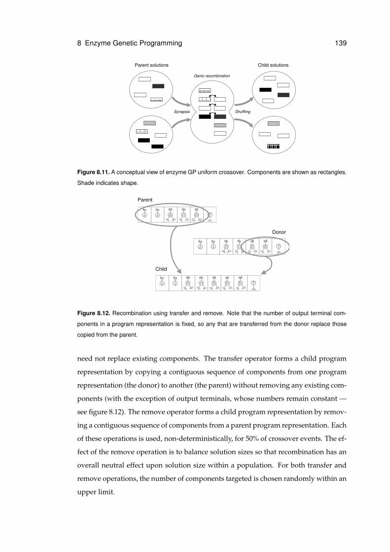
8 Enzyme Genetic Programming 139
Synapsis
Parent�solutions Child�solutions
Shuffling
Genic�recombination
Figure 8.11. A conceptual view of enzyme GP uniform crossover. Components are shown as rectangles.
Shade indicates shape.
Parent
Donor
Child
Figure 8.12. Recombination using transfer and remove. Note that the number of output terminal com-
ponents in a program representation is fixed, so any that are transferred from the donor replace those
copied from the parent.
need not replace existing components. The transfer operator forms a child program
representation by copying a contiguous sequence of components from one program
representation (the donor) to another (the parent) without removing any existing com-
ponents (with the exception of output terminals, whose numbers remain constant —
see figure 8.12). The remove operator forms a child program representation by remov-
ing a contiguous sequence of components from a parent program representation. Each
of these operations is used, non-deterministically, for 50% of crossover events. The ef-
fect of the remove operation is to balance solution sizes so that recombination has an
overall neutral effect upon solution size within a population. For both transfer and
remove operations, the number of components targeted is chosen randomly within an
upper limit.
8 Enzyme Genetic Programming 140
8.7 Summary
This chapter has introduced a form of genetic programming based upon an implicit
context program representation in which interactions between program components
are specified via behavioural descriptions rather than by position or other arbitrary
references. Implicit context representation is expected to lead to a process of meaning-
ful variation filtering whereby inappropriate change induced by variation operators
can be wholly or partially ignored as a consequence of program behaviours emerg-
ing from the self-organisation of program components — ignoring those components
which do not fit the contexts declared by the other components within the program.
9 Experimental Resultsand Analysis
This chapter presents the results of a series of experiments designed to give insight
into the performance, behaviour, and scope of enzyme genetic programming. In par-
ticular, this chapter aims to document:
• The efficacy of functionality as an implementation of implicit context.
• The performance and behaviour of recombination.
• The evolution of program size and structure.
• The role and evolution of redundancy.
• The evolution of compartmentalisation.
• The complexity and consequences of development.
• Comparative performance against other GP approaches.
9.1 Experimental Method
The implementation of enzyme GP used for this study uses a number of metrics to
measure performance and behaviour. Table 9.1 lists those which are referred to in this
chapter. Table 9.2 lists the parameters of the system, along with their default values.
Where no parameter value is given for a particular experiment, the default value is
assumed. Fitness values and run lengths are typically not normally distributed and
141
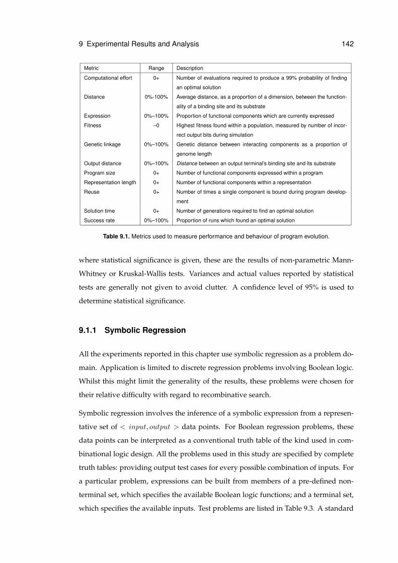
9 Experimental Results and Analysis 142
Metric Range Description
Computational effort 0+ Number of evaluations required to produce a 99% probability of finding
an optimal solution
Distance 0%-100% Average distance, as a proportion of a dimension, between the function-
ality of a binding site and its substrate
Expression 0%–100% Proportion of functional components which are currently expressed
Fitness –0 Highest fitness found within a population, measured by number of incor-
rect output bits during simulation
Genetic linkage 0%–100% Genetic distance between interacting components as a proportion of
genome length
Output distance 0%–100% Distance between an output terminal’s binding site and its substrate
Program size 0+ Number of functional components expressed within a program
Representation length 0+ Number of functional components within a representation
Reuse 0+ Number of times a single component is bound during program develop-
ment
Solution time 0+ Number of generations required to find an optimal solution
Success rate 0%–100% Proportion of runs which found an optimal solution
Table 9.1. Metrics used to measure performance and behaviour of program evolution.
where statistical significance is given, these are the results of non-parametric Mann-
Whitney or Kruskal-Wallis tests. Variances and actual values reported by statistical
tests are generally not given to avoid clutter. A confidence level of 95% is used to
determine statistical significance.
9.1.1 Symbolic Regression
All the experiments reported in this chapter use symbolic regression as a problem do-
main. Application is limited to discrete regression problems involving Boolean logic.
Whilst this might limit the generality of the results, these problems were chosen for
their relative difficulty with regard to recombinative search.
Symbolic regression involves the inference of a symbolic expression from a represen-
tative set of < input, output > data points. For Boolean regression problems, these
data points can be interpreted as a conventional truth table of the kind used in com-
binational logic design. All the problems used in this study are specified by complete
truth tables: providing output test cases for every possible combination of inputs. For
a particular problem, expressions can be built from members of a pre-defined non-
terminal set, which specifies the available Boolean logic functions; and a terminal set,
which specifies the available inputs. Test problems are listed in Table 9.3. A standard
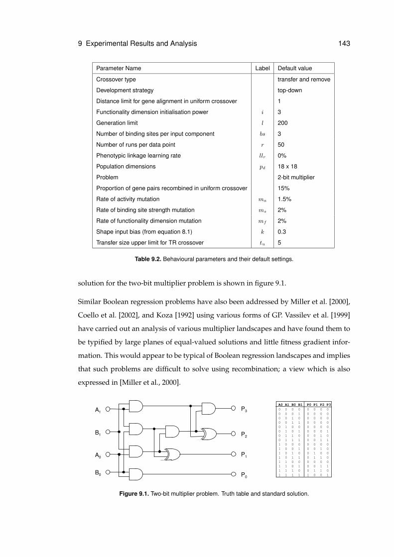
9 Experimental Results and Analysis 143
Parameter Name Label Default value
Crossover type transfer and remove
Development strategy top-down
Distance limit for gene alignment in uniform crossover 1
Functionality dimension initialisation power i 3
Generation limit l 200
Number of binding sites per input component bs 3
Number of runs per data point r 50
Phenotypic linkage learning rate llr 0%
Population dimensions pd 18 x 18
Problem 2-bit multiplier
Proportion of gene pairs recombined in uniform crossover 15%
Rate of activity mutation ma 1.5%
Rate of binding site strength mutation ms 2%
Rate of functionality dimension mutation mf 2%
Shape input bias (from equation 8.1) k 0.3
Transfer size upper limit for TR crossover tu 5
Table 9.2. Behavioural parameters and their default settings.
solution for the two-bit multiplier problem is shown in figure 9.1.
Similar Boolean regression problems have also been addressed by Miller et al. [2000],
Coello et al. [2002], and Koza [1992] using various forms of GP. Vassilev et al. [1999]
have carried out an analysis of various multiplier landscapes and have found them to
be typified by large planes of equal-valued solutions and little fitness gradient infor-
mation. This would appear to be typical of Boolean regression landscapes and implies
that such problems are difficult to solve using recombination; a view which is also
expressed in [Miller et al., 2000].
A0 A1 B0 B1 P0 P1 P2 P30 0 0 0 0 0 0 00 0 0 1 0 0 0 00 0 1 0 0 0 0 00 0 1 1 0 0 0 00 1 0 0 0 0 0 00 1 0 1 0 0 0 10 1 1 0 0 0 1 00 1 1 1 0 0 1 11 0 0 0 0 0 0 01 0 0 1 0 0 1 01 0 1 0 0 1 0 01 0 1 1 0 1 1 01 1 0 0 0 0 0 01 1 0 1 0 0 1 11 1 1 0 0 1 1 01 1 1 1 1 0 0 1
A1
B1
A0
B0
P3
P2
P1
P0
Figure 9.1. Two-bit multiplier problem. Truth table and standard solution.
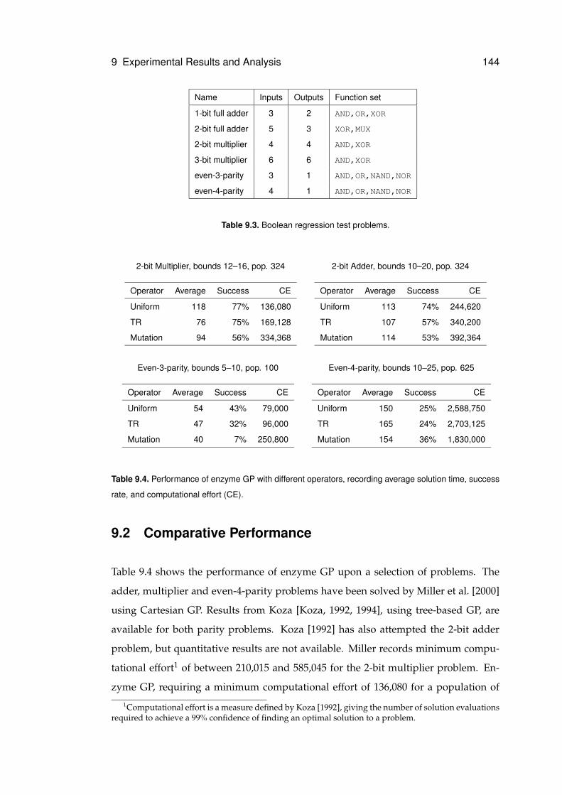
9 Experimental Results and Analysis 144
Name Inputs Outputs Function set
1-bit full adder 3 2 AND,OR,XOR
2-bit full adder 5 3 XOR,MUX
2-bit multiplier 4 4 AND,XOR
3-bit multiplier 6 6 AND,XOR
even-3-parity 3 1 AND,OR,NAND,NOR
even-4-parity 4 1 AND,OR,NAND,NOR
Table 9.3. Boolean regression test problems.
2-bit Multiplier, bounds 12–16, pop. 324
Operator Average Success CE
Uniform 118 77% 136,080
TR 76 75% 169,128
Mutation 94 56% 334,368
2-bit Adder, bounds 10–20, pop. 324
Operator Average Success CE
Uniform 113 74% 244,620
TR 107 57% 340,200
Mutation 114 53% 392,364
Even-3-parity, bounds 5–10, pop. 100
Operator Average Success CE
Uniform 54 43% 79,000
TR 47 32% 96,000
Mutation 40 7% 250,800
Even-4-parity, bounds 10–25, pop. 625
Operator Average Success CE
Uniform 150 25% 2,588,750
TR 165 24% 2,703,125
Mutation 154 36% 1,830,000
Table 9.4. Performance of enzyme GP with different operators, recording average solution time, success
rate, and computational effort (CE).
9.2 Comparative Performance
Table 9.4 shows the performance of enzyme GP upon a selection of problems. The
adder, multiplier and even-4-parity problems have been solved by Miller et al. [2000]
using Cartesian GP. Results from Koza [Koza, 1992, 1994], using tree-based GP, are
available for both parity problems. Koza [1992] has also attempted the 2-bit adder
problem, but quantitative results are not available. Miller records minimum compu-
tational effort1 of between 210,015 and 585,045 for the 2-bit multiplier problem. En-
zyme GP, requiring a minimum computational effort of 136,080 for a population of
1Computational effort is a measure defined by Koza [1992], giving the number of solution evaluationsrequired to achieve a 99% confidence of finding an optimal solution to a problem.
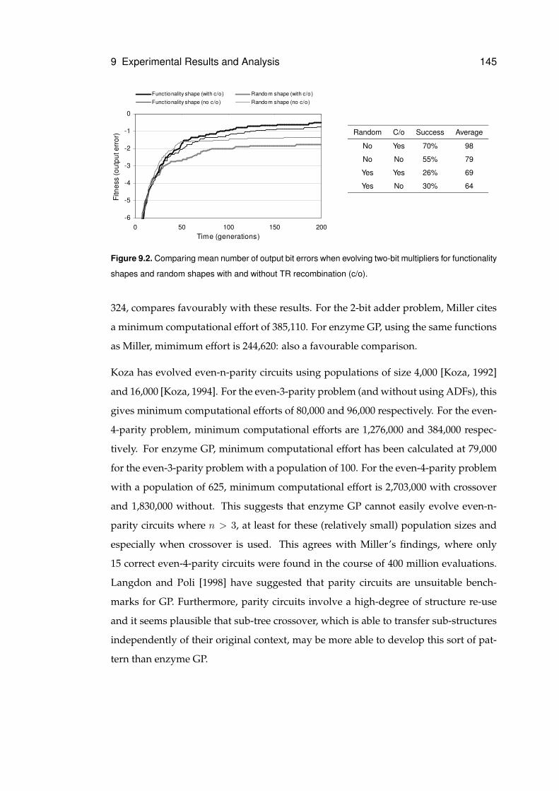
9 Experimental Results and Analysis 145
-6
-5
-4
-3
-2
-1
0
0 50 100 150 200Time (generations)
Fitn
ess
(out
put e
rror
)
Functionality shape (with c/o) Random shape (with c/o )
Functionality shape (no c/o ) Random shape (no c/o)
Random C/o Success Average
No Yes 70% 98
No No 55% 79
Yes Yes 26% 69
Yes No 30% 64
Figure 9.2. Comparing mean number of output bit errors when evolving two-bit multipliers for functionality
shapes and random shapes with and without TR recombination (c/o).
324, compares favourably with these results. For the 2-bit adder problem, Miller cites
a minimum computational effort of 385,110. For enzyme GP, using the same functions
as Miller, mimimum effort is 244,620: also a favourable comparison.
Koza has evolved even-n-parity circuits using populations of size 4,000 [Koza, 1992]
and 16,000 [Koza, 1994]. For the even-3-parity problem (and without using ADFs), this
gives minimum computational efforts of 80,000 and 96,000 respectively. For the even-
4-parity problem, minimum computational efforts are 1,276,000 and 384,000 respec-
tively. For enzyme GP, minimum computational effort has been calculated at 79,000
for the even-3-parity problem with a population of 100. For the even-4-parity problem
with a population of 625, minimum computational effort is 2,703,000 with crossover
and 1,830,000 without. This suggests that enzyme GP cannot easily evolve even-n-
parity circuits where n > 3, at least for these (relatively small) population sizes and
especially when crossover is used. This agrees with Miller’s findings, where only
15 correct even-4-parity circuits were found in the course of 400 million evaluations.
Langdon and Poli [1998] have suggested that parity circuits are unsuitable bench-
marks for GP. Furthermore, parity circuits involve a high-degree of structure re-use
and it seems plausible that sub-tree crossover, which is able to transfer sub-structures
independently of their original context, may be more able to develop this sort of pat-
tern than enzyme GP.
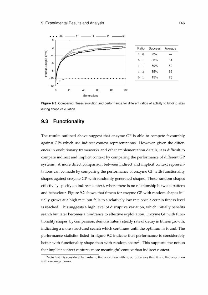
9 Experimental Results and Analysis 146
-12
-10
-8
-6
-4
-2
0
0 20 40 60 80 100
Generations
Fitn
ess
(out
put e
rror
)
1:0 3:1 1:1 1:3 0:1
Ratio Success Average
1 : 0 0% —
3 : 1 33% 51
1 : 1 50% 50
1 : 3 35% 69
0 : 1 15% 76
Figure 9.3. Comparing fitness evolution and performance for different ratios of activity to binding sites
during shape calculation.
9.3 Functionality
The results outlined above suggest that enzyme GP is able to compete favourably
against GPs which use indirect context representations. However, given the differ-
ences in evolutionary frameworks and other implementation details, it is difficult to
compare indirect and implicit context by comparing the performance of different GP
systems. A more direct comparison between indirect and implicit context represen-
tations can be made by comparing the performance of enzyme GP with functionality
shapes against enzyme GP with randomly generated shapes. These random shapes
effectively specify an indirect context, where there is no relationship between pattern
and behaviour. Figure 9.2 shows that fitness for enzyme GP with random shapes ini-
tially grows at a high rate, but falls to a relatively low rate once a certain fitness level
is reached. This suggests a high level of disruptive variation, which initially benefits
search but later becomes a hindrance to effective exploitation. Enzyme GP with func-
tionality shapes, by comparison, demonstrates a steady rate of decay in fitness growth,
indicating a more structured search which continues until the optimum is found. The
performance statistics listed in figure 9.2 indicate that performance is considerably
better with functionality shape than with random shape2. This supports the notion
that implicit context captures more meaningful context than indirect context.
2Note that it is considerably harder to find a solution with no output errors than it is to find a solutionwith one output error.
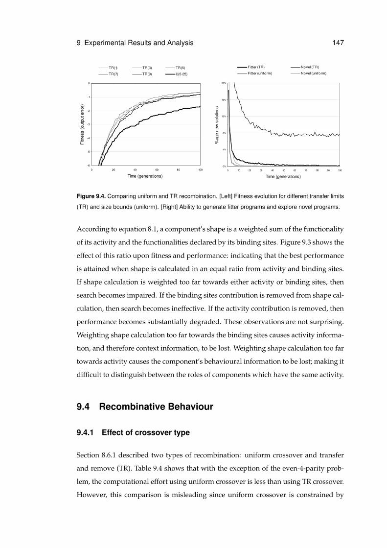
9 Experimental Results and Analysis 147
-6
-5
-4
-3
-2
-1
0
0 20 40 60 80 100
Time (generations)
Fitn
ess
(out
put e
rror
)
TR(1) TR(3) TR(5)
TR(7) TR(9) U(5-25)
0%
4%
8%
12%
16%
20%
0 10 20 30 40 50 60 70 80 90 100
Time (generations)
%ag
e ne
w s
olut
ions
Fitter (TR) Novel (TR)
Fitter (unifo rm) Novel (unifo rm)
Figure 9.4. Comparing uniform and TR recombination. [Left] Fitness evolution for different transfer limits
(TR) and size bounds (uniform). [Right] Ability to generate fitter programs and explore novel programs.
According to equation 8.1, a component’s shape is a weighted sum of the functionality
of its activity and the functionalities declared by its binding sites. Figure 9.3 shows the
effect of this ratio upon fitness and performance: indicating that the best performance
is attained when shape is calculated in an equal ratio from activity and binding sites.
If shape calculation is weighted too far towards either activity or binding sites, then
search becomes impaired. If the binding sites contribution is removed from shape cal-
culation, then search becomes ineffective. If the activity contribution is removed, then
performance becomes substantially degraded. These observations are not surprising.
Weighting shape calculation too far towards the binding sites causes activity informa-
tion, and therefore context information, to be lost. Weighting shape calculation too far
towards activity causes the component’s behavioural information to be lost; making it
difficult to distinguish between the roles of components which have the same activity.
9.4 Recombinative Behaviour
9.4.1 Effect of crossover type
Section 8.6.1 described two types of recombination: uniform crossover and transfer
and remove (TR). Table 9.4 shows that with the exception of the even-4-parity prob-
lem, the computational effort using uniform crossover is less than using TR crossover.
However, this comparison is misleading since uniform crossover is constrained by
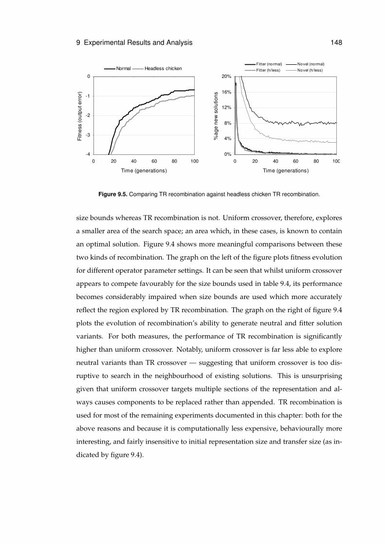
9 Experimental Results and Analysis 148
-4
-3
-2
-1
0
0 20 40 60 80 100
Time (generations)
Fitn
ess
(out
put e
rror
)
Normal Headless chicken
0%
4%
8%
12%
16%
20%
0 20 40 60 80 100
Time (generations)
%ag
e ne
w s
olut
ions
Fitter (normal) Novel (normal)
Fitter (h/less) Novel (h/less)
Figure 9.5. Comparing TR recombination against headless chicken TR recombination.
size bounds whereas TR recombination is not. Uniform crossover, therefore, explores
a smaller area of the search space; an area which, in these cases, is known to contain
an optimal solution. Figure 9.4 shows more meaningful comparisons between these
two kinds of recombination. The graph on the left of the figure plots fitness evolution
for different operator parameter settings. It can be seen that whilst uniform crossover
appears to compete favourably for the size bounds used in table 9.4, its performance
becomes considerably impaired when size bounds are used which more accurately
reflect the region explored by TR recombination. The graph on the right of figure 9.4
plots the evolution of recombination’s ability to generate neutral and fitter solution
variants. For both measures, the performance of TR recombination is significantly
higher than uniform crossover. Notably, uniform crossover is far less able to explore
neutral variants than TR crossover — suggesting that uniform crossover is too dis-
ruptive to search in the neighbourhood of existing solutions. This is unsurprising
given that uniform crossover targets multiple sections of the representation and al-
ways causes components to be replaced rather than appended. TR recombination is
used for most of the remaining experiments documented in this chapter: both for the
above reasons and because it is computationally less expensive, behaviourally more
interesting, and fairly insensitive to initial representation size and transfer size (as in-
dicated by figure 9.4).
9 Experimental Results and Analysis 149
9.4.2 Crossover versus Mutation
According to the arguments described in [Vassilev et al., 1999], recombination would
be expected to offer relatively poor performance upon Boolean symbolic regression
problems. For this reason, recombination was not used in Miller’s experiments on
digital circuit evolution [Miller et al., 2000]. However, results from experiments using
enzyme GP indicate that recombination can play an important role in digital circuit
evolution and, significantly, offers better search performance than mutation opera-
tors. Table 9.4 shows that, in all but the even-4-parity problem, enzyme GP with re-
combination performs considerably better than enzyme GP with mutation alone. In
previous GP studies, headless chicken crossover operators, which recombine existing
solutions with randomly generated solutions, have been used to show that crossover
performs no better than macro-mutation. Results depicted in figure 9.5 show that for
enzyme GP, TR recombination offers better performance than a headless chicken op-
erator based upon TR recombination. This suggests that recombination is transferring
useful information between programs. However, even the headless variant offers rea-
sonable performance.
A more direct comparison between the search performance of recombination and mu-
tation has been carried out by configuring enzyme GP’s evolutionary framework to
generate one child via recombination and another via mutation for every reproduction
event and by measuring the relative fitness of the children produced by each opera-
tor. This was done for both functionality and random shapes. Figure 9.6 shows that
when functionality shapes are used, recombination is responsible for generating the
fittest child during a substantially greater proportion of reproduction events than mu-
tation. This suggests that recombination has considerably more influence upon search
than mutation. However, when random shapes are used, recombination is no longer
the dominant operator with (especially for the multiplier problem) mutation gener-
ating the greater proportion of fitter children during reproduction events. This lends
weight to the argument that implicit context improves the behaviour of recombination
with respect to indirect context. Figure 9.6 also shows that transfer operations have a
slightly higher success rate than remove operations during TR recombination. This re-
flects the fact that solutions are more likely to be disrupted by removing components
than they are by gaining components.
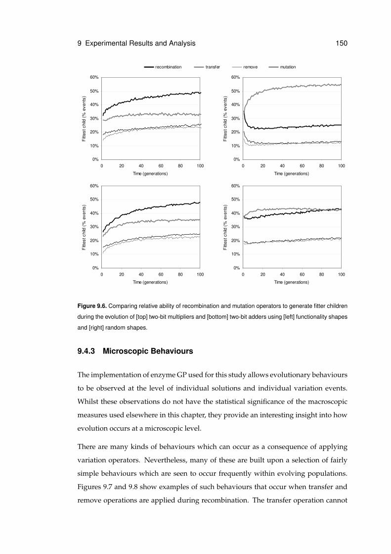
9 Experimental Results and Analysis 150
0%
10%
20%
30%
40%
50%
60%
0 20 40 60 80 100
Time (generations)
Fitt
est c
hild
(%
eve
nts)
0%
10%
20%
30%
40%
50%
60%
0 20 40 60 80 100
Time (generations)
Fitt
est c
hild
(%
eve
nts)
0%
10%
20%
30%
40%
50%
60%
0 20 40 60 80 100
Time (generations)
Fitt
est c
hild
(%
eve
nts)
0%
10%
20%
30%
40%
50%
60%
0 20 40 60 80 100
Time (generations)
Fitt
est c
hild
(%
eve
nts)
recombination transfer remove mutation
Figure 9.6. Comparing relative ability of recombination and mutation operators to generate fitter children
during the evolution of [top] two-bit multipliers and [bottom] two-bit adders using [left] functionality shapes
and [right] random shapes.
9.4.3 Microscopic Behaviours
The implementation of enzyme GP used for this study allows evolutionary behaviours
to be observed at the level of individual solutions and individual variation events.
Whilst these observations do not have the statistical significance of the macroscopic
measures used elsewhere in this chapter, they provide an interesting insight into how
evolution occurs at a microscopic level.
There are many kinds of behaviours which can occur as a consequence of applying
variation operators. Nevertheless, many of these are built upon a selection of fairly
simple behaviours which are seen to occur frequently within evolving populations.
Figures 9.7 and 9.8 show examples of such behaviours that occur when transfer and
remove operations are applied during recombination. The transfer operation cannot
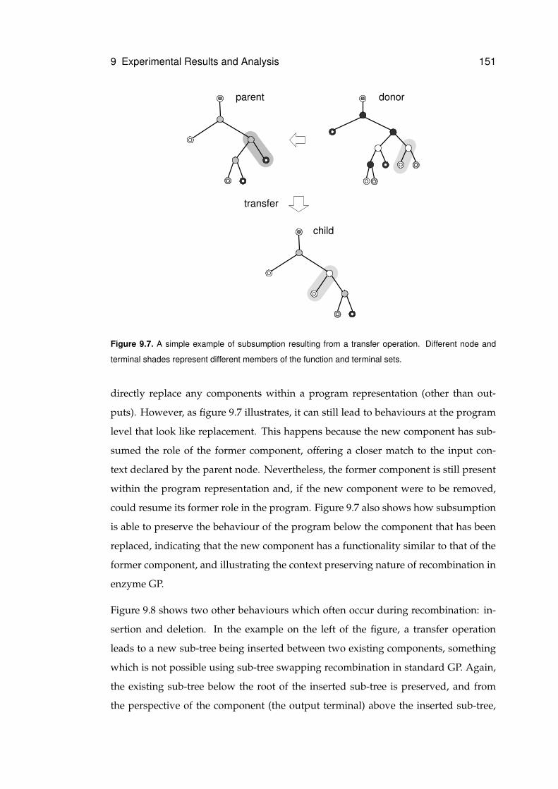
9 Experimental Results and Analysis 151
parent
transfer
child
donor
Figure 9.7. A simple example of subsumption resulting from a transfer operation. Different node and
terminal shades represent different members of the function and terminal sets.
directly replace any components within a program representation (other than out-
puts). However, as figure 9.7 illustrates, it can still lead to behaviours at the program
level that look like replacement. This happens because the new component has sub-
sumed the role of the former component, offering a closer match to the input con-
text declared by the parent node. Nevertheless, the former component is still present
within the program representation and, if the new component were to be removed,
could resume its former role in the program. Figure 9.7 also shows how subsumption
is able to preserve the behaviour of the program below the component that has been
replaced, indicating that the new component has a functionality similar to that of the
former component, and illustrating the context preserving nature of recombination in
enzyme GP.
Figure 9.8 shows two other behaviours which often occur during recombination: in-
sertion and deletion. In the example on the left of the figure, a transfer operation
leads to a new sub-tree being inserted between two existing components, something
which is not possible using sub-tree swapping recombination in standard GP. Again,
the existing sub-tree below the root of the inserted sub-tree is preserved, and from
the perspective of the component (the output terminal) above the inserted sub-tree,
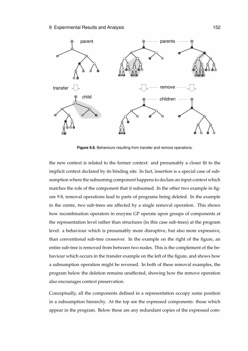
9 Experimental Results and Analysis 152
parent
transfer
child
parents
children
remove
Figure 9.8. Behaviours resulting from transfer and remove operations.
the new context is related to the former context: and presumably a closer fit to the
implicit context declared by its binding site. In fact, insertion is a special case of sub-
sumption where the subsuming component happens to declare an input context which
matches the role of the component that it subsumed. In the other two example in fig-
ure 9.8, removal operations lead to parts of programs being deleted. In the example
in the centre, two sub-trees are affected by a single removal operation. This shows
how recombination operators in enzyme GP operate upon groups of components at
the representation level rather than structures (in this case sub-trees) at the program
level: a behaviour which is presumably more disruptive, but also more expressive,
than conventional sub-tree crossover. In the example on the right of the figure, an
entire sub-tree is removed from between two nodes. This is the complement of the be-
haviour which occurs in the transfer example on the left of the figure, and shows how
a subsumption operation might be reversed. In both of these removal examples, the
program below the deletion remains unaffected, showing how the remove operation
also encourages context preservation.
Conceptually, all the components defined in a representation occupy some position
in a subsumption hierarchy. At the top are the expressed components: those which
appear in the program. Below these are any redundant copies of the expressed com-
9 Experimental Results and Analysis 153
ponents. Below these are components that have been subsumed by the expressed
components; and further down, components that were subsumed by components fur-
ther up the hierarchy which have since themselves also been subsumed. At the bot-
tom are components which have never been expressed but which could in principle
be expressed if all the components above them in the subsumption hierarchy were
removed. All the behaviours that occur in enzyme GP are a result of variation op-
erators modifying this subsumption hierarchy: either by adding new entries, by re-
moving entries or by re-ordering existing entries (which is what mutation operators
are essentially doing). Nevertheless, the operators are not aware of this subsumption
hierarchy. They blindly add, remove and re-order entries — only causing change in
the program when they happen to add, remove or re-order entries at the top of the
hierarchy. All other changes are absorbed into the lower echelons of the hierarchy.
Subsumption supports the idea that the program representation used by enzyme GP
promotes meaningful variation filtering: since it is clearly the way in which the repre-
sentation describes the program, rather than the action of the variation operators, that
allows subsumptive behaviours to occur.
9.5 Size Evolution
In general, enzyme GP produces little or no bloat in both representation and program
size. Figure 9.9 shows the size evolution of two-bit multipliers for both recombina-
tion operators and for different initial representation sizes. Size evolution under TR
recombination is of particular interest, since in principal there is no upper bound to
solution length. Nevertheless, there appears to be little pressure for the recombination
operators to explore representation lengths much larger than the initial representation
length. What little amount of growth there is for an initial representation length of 15
components can readily be accounted for either by the differential performance of the
transfer and remove operators3, by an initial representation length insufficient to eas-
ily express optimal solutions, or by there being many more solution representations
of greater length than the initial representation length (or shorter). However, for an
initial representation length of 30 components, even these factors appear to have no
effect upon representation length.3This is akin to the removal bias cause of bloat seen in tree-based GP.
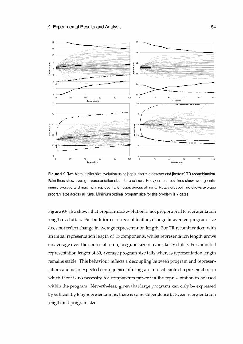
9 Experimental Results and Analysis 154
4
5
6
7
8
9
10
11
12
0 20 40 60 80 100
Generations
Sol
utio
n�si
ze
10
14
18
22
26
30
0 20 40 60 80 100
Generations
Sol
utio
n�si
ze
0
10
20
30
40
50
0 20 40 60 80 100
Generations
Sol
utio
n�si
ze
0
10
20
30
40
50
0 20 40 60 80 100
Generations
So
luti
on
�Siz
e
Figure 9.9. Two-bit multiplier size evolution using [top] uniform crossover and [bottom] TR recombination.
Faint lines show average representation sizes for each run. Heavy un-crossed lines show average min-
imum, average and maximum representation sizes across all runs. Heavy crossed line shows average
program size across all runs. Minimum optimal program size for this problem is 7 gates.
Figure 9.9 also shows that program size evolution is not proportional to representation
length evolution. For both forms of recombination, change in average program size
does not reflect change in average representation length. For TR recombination: with
an initial representation length of 15 components, whilst representation length grows
on average over the course of a run, program size remains fairly stable. For an initial
representation length of 30, average program size falls whereas representation length
remains stable. This behaviour reflects a decoupling between program and represen-
tation; and is an expected consequence of using an implicit context representation in
which there is no necessity for components present in the representation to be used
within the program. Nevertheless, given that large programs can only be expressed
by sufficiently long representations, there is some dependence between representation
length and program size.
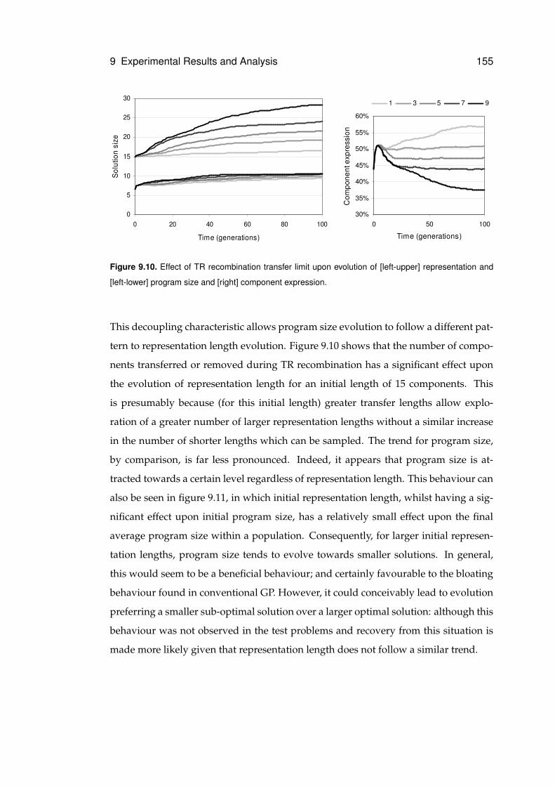
9 Experimental Results and Analysis 155
0
5
10
15
20
25
30
0 20 40 60 80 100
Time (generations)
Sol
utio
n si
ze
30%
35%
40%
45%
50%
55%
60%
0 50 100
Time (generations)
Com
pone
nt e
xpre
ssio
n
1 3 5 7 9
Figure 9.10. Effect of TR recombination transfer limit upon evolution of [left-upper] representation and
[left-lower] program size and [right] component expression.
This decoupling characteristic allows program size evolution to follow a different pat-
tern to representation length evolution. Figure 9.10 shows that the number of compo-
nents transferred or removed during TR recombination has a significant effect upon
the evolution of representation length for an initial length of 15 components. This
is presumably because (for this initial length) greater transfer lengths allow explo-
ration of a greater number of larger representation lengths without a similar increase
in the number of shorter lengths which can be sampled. The trend for program size,
by comparison, is far less pronounced. Indeed, it appears that program size is at-
tracted towards a certain level regardless of representation length. This behaviour can
also be seen in figure 9.11, in which initial representation length, whilst having a sig-
nificant effect upon initial program size, has a relatively small effect upon the final
average program size within a population. Consequently, for larger initial represen-
tation lengths, program size tends to evolve towards smaller solutions. In general,
this would seem to be a beneficial behaviour; and certainly favourable to the bloating
behaviour found in conventional GP. However, it could conceivably lead to evolution
preferring a smaller sub-optimal solution over a larger optimal solution: although this
behaviour was not observed in the test problems and recovery from this situation is
made more likely given that representation length does not follow a similar trend.
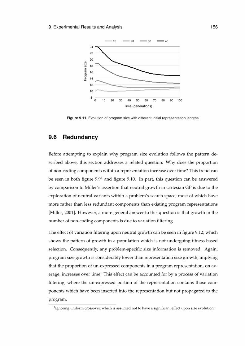
9 Experimental Results and Analysis 156
8
10
12
14
16
18
20
22
24
0 10 20 30 40 50 60 70 80 90 100
Time (generations)
Pro
gram
siz
e
15 20 30 40
Figure 9.11. Evolution of program size with different initial representation lengths.
9.6 Redundancy
Before attempting to explain why program size evolution follows the pattern de-
scribed above, this section addresses a related question: Why does the proportion
of non-coding components within a representation increase over time? This trend can
be seen in both figure 9.94 and figure 9.10. In part, this question can be answered
by comparison to Miller’s assertion that neutral growth in cartesian GP is due to the
exploration of neutral variants within a problem’s search space; most of which have
more rather than less redundant components than existing program representations
[Miller, 2001]. However, a more general answer to this question is that growth in the
number of non-coding components is due to variation filtering.
The effect of variation filtering upon neutral growth can be seen in figure 9.12; which
shows the pattern of growth in a population which is not undergoing fitness-based
selection. Consequently, any problem-specific size information is removed. Again,
program size growth is considerably lower than representation size growth, implying
that the proportion of un-expressed components in a program representation, on av-
erage, increases over time. This effect can be accounted for by a process of variation
filtering, where the un-expressed portion of the representation contains those com-
ponents which have been inserted into the representation but not propagated to the
program.
4Ignoring uniform crossover, which is assumed not to have a significant effect upon size evolution.
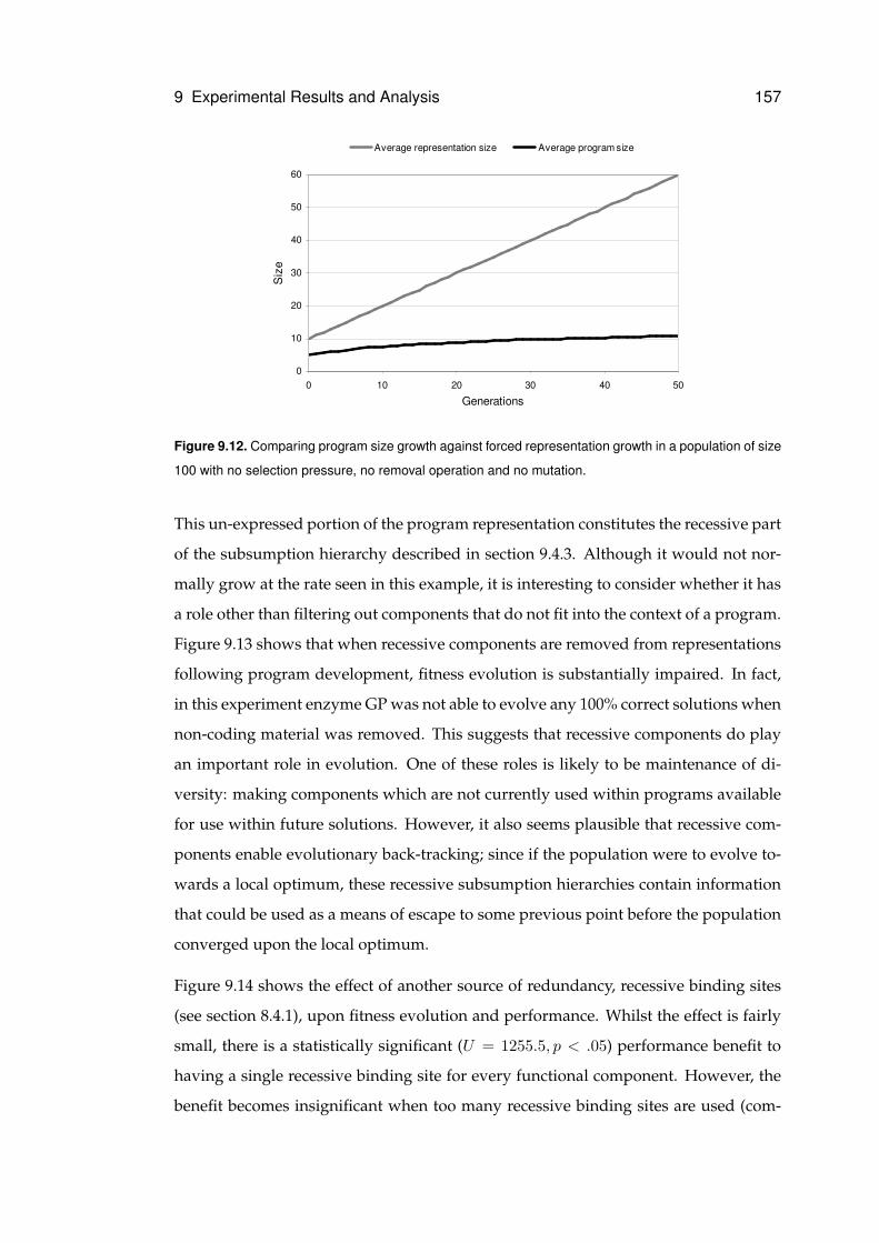
9 Experimental Results and Analysis 157
0
10
20
30
40
50
60
0 10 20 30 40 50
Generations
Siz
e
Average representation size Average program size
Figure 9.12. Comparing program size growth against forced representation growth in a population of size
100 with no selection pressure, no removal operation and no mutation.
This un-expressed portion of the program representation constitutes the recessive part
of the subsumption hierarchy described in section 9.4.3. Although it would not nor-
mally grow at the rate seen in this example, it is interesting to consider whether it has
a role other than filtering out components that do not fit into the context of a program.
Figure 9.13 shows that when recessive components are removed from representations
following program development, fitness evolution is substantially impaired. In fact,
in this experiment enzyme GP was not able to evolve any 100% correct solutions when
non-coding material was removed. This suggests that recessive components do play
an important role in evolution. One of these roles is likely to be maintenance of di-
versity: making components which are not currently used within programs available
for use within future solutions. However, it also seems plausible that recessive com-
ponents enable evolutionary back-tracking; since if the population were to evolve to-
wards a local optimum, these recessive subsumption hierarchies contain information
that could be used as a means of escape to some previous point before the population
converged upon the local optimum.
Figure 9.14 shows the effect of another source of redundancy, recessive binding sites
(see section 8.4.1), upon fitness evolution and performance. Whilst the effect is fairly
small, there is a statistically significant (U = 1255.5, p < .05) performance benefit to
having a single recessive binding site for every functional component. However, the
benefit becomes insignificant when too many recessive binding sites are used (com-
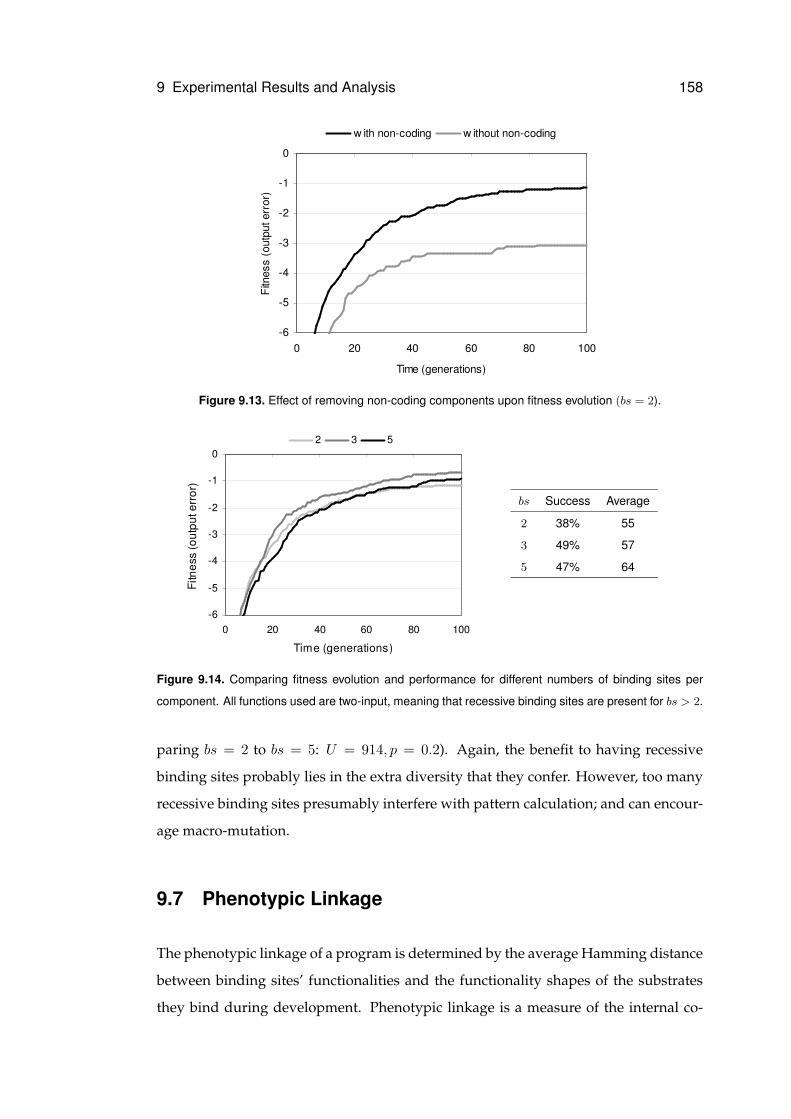
9 Experimental Results and Analysis 158
-6
-5
-4
-3
-2
-1
0
0 20 40 60 80 100
Time (generations)
Fitn
ess
(out
put e
rror
)
w ith non-coding w ithout non-coding
Figure 9.13. Effect of removing non-coding components upon fitness evolution (bs = 2).
-6
-5
-4
-3
-2
-1
0
0 20 40 60 80 100
Time (generations)
Fitn
ess
(out
put e
rror
)
2 3 5
bs Success Average
2 38% 55
3 49% 57
5 47% 64
Figure 9.14. Comparing fitness evolution and performance for different numbers of binding sites per
component. All functions used are two-input, meaning that recessive binding sites are present for bs > 2.
paring bs = 2 to bs = 5: U = 914, p = 0.2). Again, the benefit to having recessive
binding sites probably lies in the extra diversity that they confer. However, too many
recessive binding sites presumably interfere with pattern calculation; and can encour-
age macro-mutation.
9.7 Phenotypic Linkage
The phenotypic linkage of a program is determined by the average Hamming distance
between binding sites’ functionalities and the functionality shapes of the substrates
they bind during development. Phenotypic linkage is a measure of the internal co-
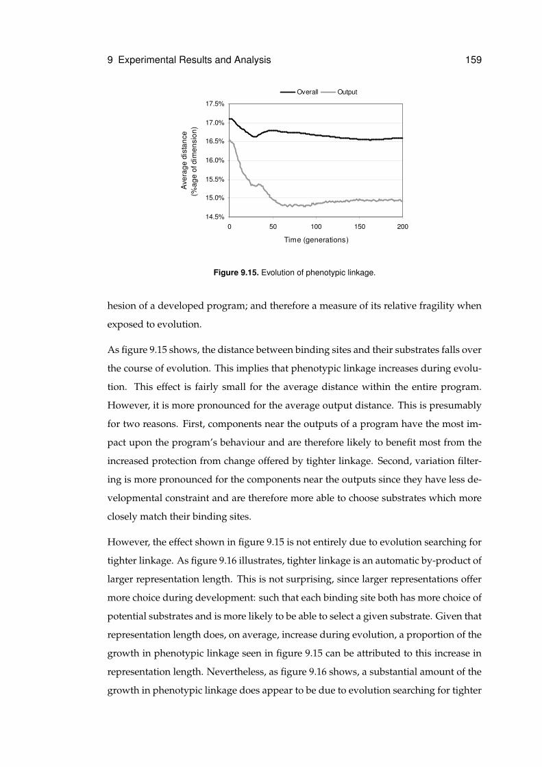
9 Experimental Results and Analysis 159
14.5%
15.0%
15.5%
16.0%
16.5%
17.0%
17.5%
0 50 100 150 200
Time (generations)
Ave
rage
dis
tanc
e(%
age
of d
imen
sion
)
Overall Output
Figure 9.15. Evolution of phenotypic linkage.
hesion of a developed program; and therefore a measure of its relative fragility when
exposed to evolution.
As figure 9.15 shows, the distance between binding sites and their substrates falls over
the course of evolution. This implies that phenotypic linkage increases during evolu-
tion. This effect is fairly small for the average distance within the entire program.
However, it is more pronounced for the average output distance. This is presumably
for two reasons. First, components near the outputs of a program have the most im-
pact upon the program’s behaviour and are therefore likely to benefit most from the
increased protection from change offered by tighter linkage. Second, variation filter-
ing is more pronounced for the components near the outputs since they have less de-
velopmental constraint and are therefore more able to choose substrates which more
closely match their binding sites.
However, the effect shown in figure 9.15 is not entirely due to evolution searching for
tighter linkage. As figure 9.16 illustrates, tighter linkage is an automatic by-product of
larger representation length. This is not surprising, since larger representations offer
more choice during development: such that each binding site both has more choice of
potential substrates and is more likely to be able to select a given substrate. Given that
representation length does, on average, increase during evolution, a proportion of the
growth in phenotypic linkage seen in figure 9.15 can be attributed to this increase in
representation length. Nevertheless, as figure 9.16 shows, a substantial amount of the
growth in phenotypic linkage does appear to be due to evolution searching for tighter
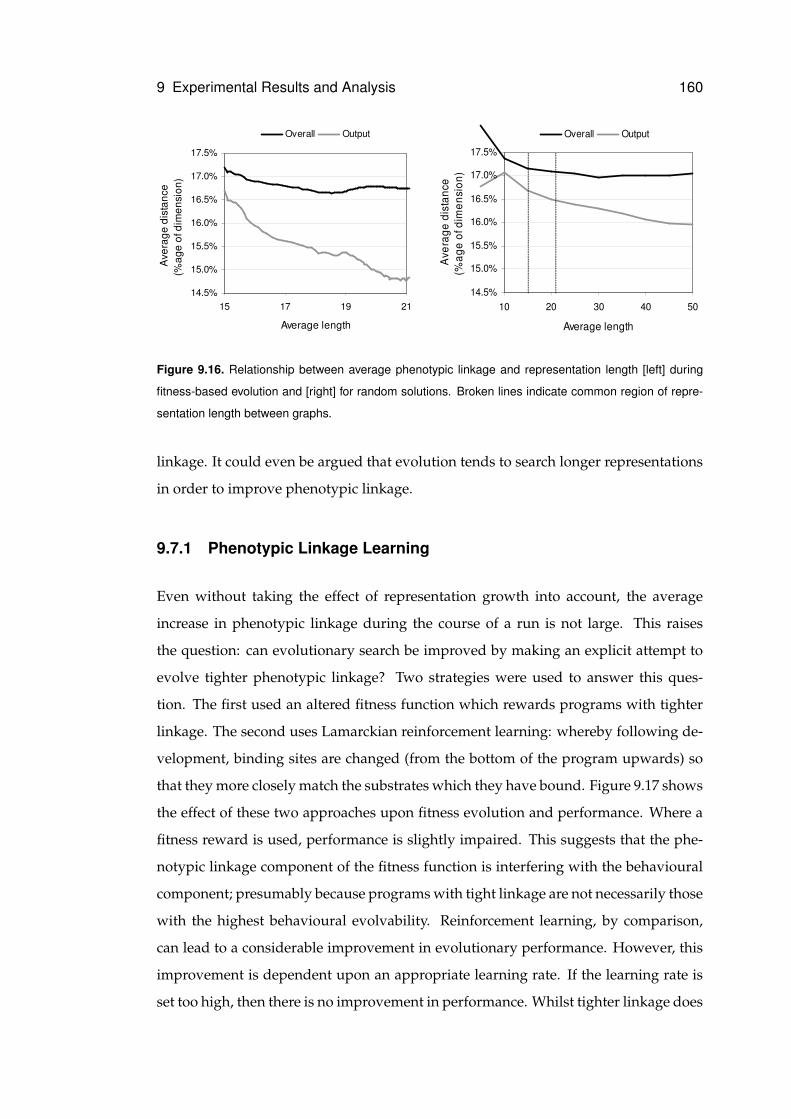
9 Experimental Results and Analysis 160
14.5%
15.0%
15.5%
16.0%
16.5%
17.0%
17.5%
15 17 19 21
Average length
Ave
rage
dis
tanc
e(%
age
of d
imen
sion
)
Overall Output
14.5%
15.0%
15.5%
16.0%
16.5%
17.0%
17.5%
10 20 30 40 50
Average length
Ave
rage
dis
tanc
e(%
age
of d
imen
sion
)
Overall Output
Figure 9.16. Relationship between average phenotypic linkage and representation length [left] during
fitness-based evolution and [right] for random solutions. Broken lines indicate common region of repre-
sentation length between graphs.
linkage. It could even be argued that evolution tends to search longer representations
in order to improve phenotypic linkage.
9.7.1 Phenotypic Linkage Learning
Even without taking the effect of representation growth into account, the average
increase in phenotypic linkage during the course of a run is not large. This raises
the question: can evolutionary search be improved by making an explicit attempt to
evolve tighter phenotypic linkage? Two strategies were used to answer this ques-
tion. The first used an altered fitness function which rewards programs with tighter
linkage. The second uses Lamarckian reinforcement learning: whereby following de-
velopment, binding sites are changed (from the bottom of the program upwards) so
that they more closely match the substrates which they have bound. Figure 9.17 shows
the effect of these two approaches upon fitness evolution and performance. Where a
fitness reward is used, performance is slightly impaired. This suggests that the phe-
notypic linkage component of the fitness function is interfering with the behavioural
component; presumably because programs with tight linkage are not necessarily those
with the highest behavioural evolvability. Reinforcement learning, by comparison,
can lead to a considerable improvement in evolutionary performance. However, this
improvement is dependent upon an appropriate learning rate. If the learning rate is
set too high, then there is no improvement in performance. Whilst tighter linkage does
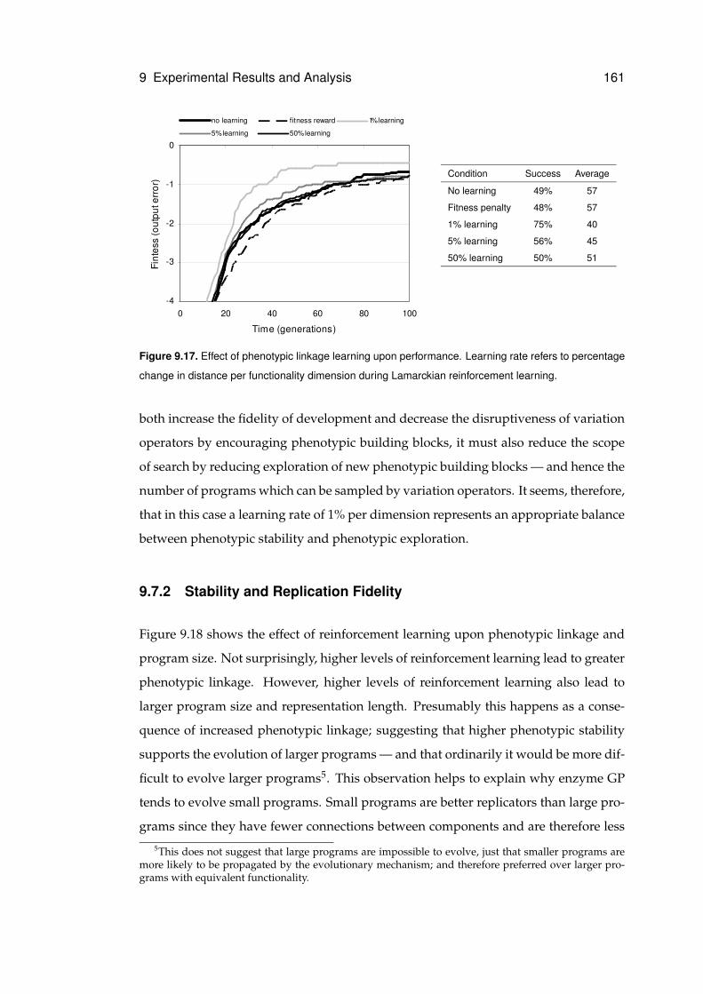
9 Experimental Results and Analysis 161
-4
-3
-2
-1
0
0 20 40 60 80 100
Time (generations)
Fint
ess
(out
put e
rror
)
no learning fitness reward 1% learning
5% learning 50% learning
Condition Success Average
No learning 49% 57
Fitness penalty 48% 57
1% learning 75% 40
5% learning 56% 45
50% learning 50% 51
Figure 9.17. Effect of phenotypic linkage learning upon performance. Learning rate refers to percentage
change in distance per functionality dimension during Lamarckian reinforcement learning.
both increase the fidelity of development and decrease the disruptiveness of variation
operators by encouraging phenotypic building blocks, it must also reduce the scope
of search by reducing exploration of new phenotypic building blocks — and hence the
number of programs which can be sampled by variation operators. It seems, therefore,
that in this case a learning rate of 1% per dimension represents an appropriate balance
between phenotypic stability and phenotypic exploration.
9.7.2 Stability and Replication Fidelity
Figure 9.18 shows the effect of reinforcement learning upon phenotypic linkage and
program size. Not surprisingly, higher levels of reinforcement learning lead to greater
phenotypic linkage. However, higher levels of reinforcement learning also lead to
larger program size and representation length. Presumably this happens as a conse-
quence of increased phenotypic linkage; suggesting that higher phenotypic stability
supports the evolution of larger programs — and that ordinarily it would be more dif-
ficult to evolve larger programs5. This observation helps to explain why enzyme GP
tends to evolve small programs. Small programs are better replicators than large pro-
grams since they have fewer connections between components and are therefore less
5This does not suggest that large programs are impossible to evolve, just that smaller programs aremore likely to be propagated by the evolutionary mechanism; and therefore preferred over larger pro-grams with equivalent functionality.
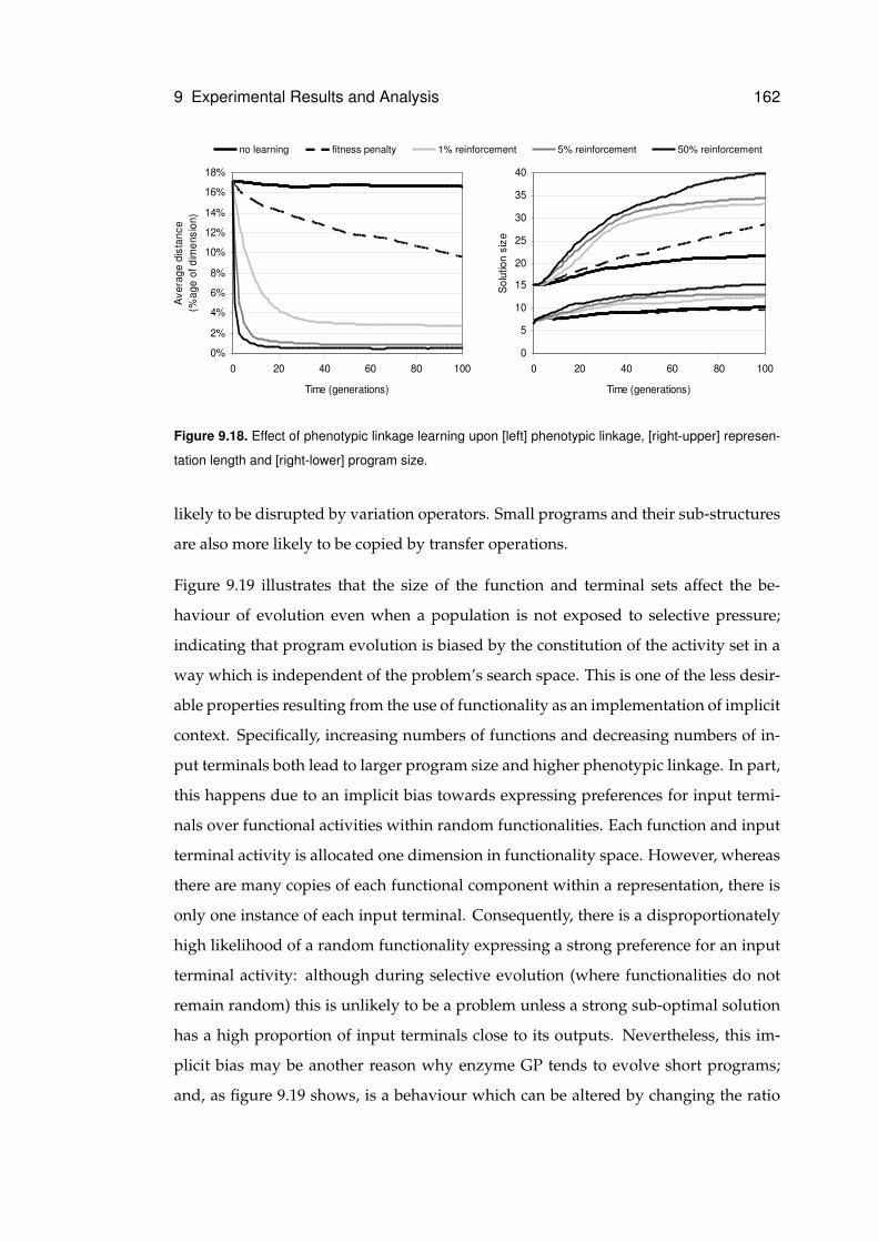
9 Experimental Results and Analysis 162
0
5
10
15
20
25
30
35
40
0 20 40 60 80 100
Time (generations)
Sol
utio
n si
ze
0%
2%
4%
6%
8%
10%
12%
14%
16%
18%
0 20 40 60 80 100
Time (generations)
Ave
rage
dis
tanc
e(%
age
of d
imen
sion
)
no learning fitness penalty 1% reinforcement 5% reinforcement 50% reinforcement
Figure 9.18. Effect of phenotypic linkage learning upon [left] phenotypic linkage, [right-upper] represen-
tation length and [right-lower] program size.
likely to be disrupted by variation operators. Small programs and their sub-structures
are also more likely to be copied by transfer operations.
Figure 9.19 illustrates that the size of the function and terminal sets affect the be-
haviour of evolution even when a population is not exposed to selective pressure;
indicating that program evolution is biased by the constitution of the activity set in a
way which is independent of the problem’s search space. This is one of the less desir-
able properties resulting from the use of functionality as an implementation of implicit
context. Specifically, increasing numbers of functions and decreasing numbers of in-
put terminals both lead to larger program size and higher phenotypic linkage. In part,
this happens due to an implicit bias towards expressing preferences for input termi-
nals over functional activities within random functionalities. Each function and input
terminal activity is allocated one dimension in functionality space. However, whereas
there are many copies of each functional component within a representation, there is
only one instance of each input terminal. Consequently, there is a disproportionately
high likelihood of a random functionality expressing a strong preference for an input
terminal activity: although during selective evolution (where functionalities do not
remain random) this is unlikely to be a problem unless a strong sub-optimal solution
has a high proportion of input terminals close to its outputs. Nevertheless, this im-
plicit bias may be another reason why enzyme GP tends to evolve short programs;
and, as figure 9.19 shows, is a behaviour which can be altered by changing the ratio
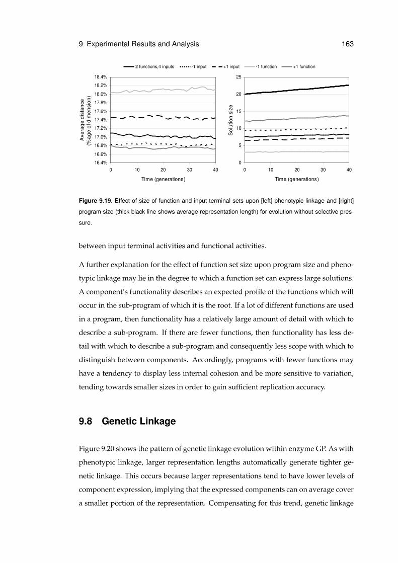
9 Experimental Results and Analysis 163
0
5
10
15
20
25
0 10 20 30 40
Time (generations)
Sol
utio
n si
ze
16.4%
16.6%
16.8%
17.0%
17.2%
17.4%
17.6%
17.8%
18.0%
18.2%
18.4%
0 10 20 30 40
Time (generations)
Ave
rage
dis
tanc
e(%
age
of d
imen
sion
)
2 functions,4 inputs -1 input +1 input -1 function +1 function
Figure 9.19. Effect of size of function and input terminal sets upon [left] phenotypic linkage and [right]
program size (thick black line shows average representation length) for evolution without selective pres-
sure.
between input terminal activities and functional activities.
A further explanation for the effect of function set size upon program size and pheno-
typic linkage may lie in the degree to which a function set can express large solutions.
A component’s functionality describes an expected profile of the functions which will
occur in the sub-program of which it is the root. If a lot of different functions are used
in a program, then functionality has a relatively large amount of detail with which to
describe a sub-program. If there are fewer functions, then functionality has less de-
tail with which to describe a sub-program and consequently less scope with which to
distinguish between components. Accordingly, programs with fewer functions may
have a tendency to display less internal cohesion and be more sensitive to variation,
tending towards smaller sizes in order to gain sufficient replication accuracy.
9.8 Genetic Linkage
Figure 9.20 shows the pattern of genetic linkage evolution within enzyme GP. As with
phenotypic linkage, larger representation lengths automatically generate tighter ge-
netic linkage. This occurs because larger representations tend to have lower levels of
component expression, implying that the expressed components can on average cover
a smaller portion of the representation. Compensating for this trend, genetic linkage
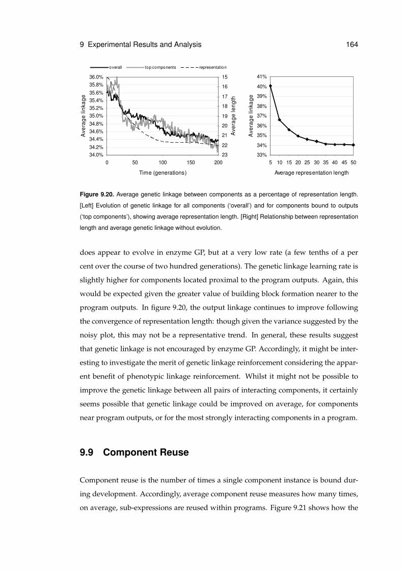
9 Experimental Results and Analysis 164
34.0%34.2%34.4%34.6%34.8%35.0%35.2%35.4%35.6%35.8%36.0%
0 50 100 150 200
Time (generations)
Ave
rage
link
age
15
16
17
18
19
20
21
22
23
Ave
rage
leng
th
overall top components representation
j
33%
34%
35%
36%
37%
38%
39%
40%
41%
5 10 15 20 25 30 35 40 45 50
Average representation length
Ave
rage
link
age
Figure 9.20. Average genetic linkage between components as a percentage of representation length.
[Left] Evolution of genetic linkage for all components (‘overall’) and for components bound to outputs
(‘top components’), showing average representation length. [Right] Relationship between representation
length and average genetic linkage without evolution.
does appear to evolve in enzyme GP, but at a very low rate (a few tenths of a per
cent over the course of two hundred generations). The genetic linkage learning rate is
slightly higher for components located proximal to the program outputs. Again, this
would be expected given the greater value of building block formation nearer to the
program outputs. In figure 9.20, the output linkage continues to improve following
the convergence of representation length: though given the variance suggested by the
noisy plot, this may not be a representative trend. In general, these results suggest
that genetic linkage is not encouraged by enzyme GP. Accordingly, it might be inter-
esting to investigate the merit of genetic linkage reinforcement considering the appar-
ent benefit of phenotypic linkage reinforcement. Whilst it might not be possible to
improve the genetic linkage between all pairs of interacting components, it certainly
seems possible that genetic linkage could be improved on average, for components
near program outputs, or for the most strongly interacting components in a program.
9.9 Component Reuse
Component reuse is the number of times a single component instance is bound dur-
ing development. Accordingly, average component reuse measures how many times,
on average, sub-expressions are reused within programs. Figure 9.21 shows how the
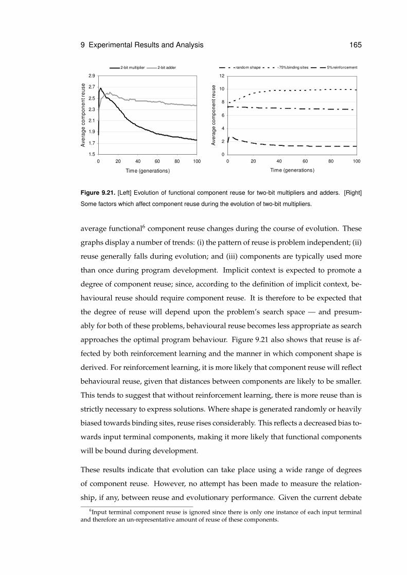
9 Experimental Results and Analysis 165
1.5
1.7
1.9
2.1
2.3
2.5
2.7
2.9
0 20 40 60 80 100
Time (generations)
Ave
rage
com
pone
nt re
use
2-bit multiplier 2-bit adder
0
2
4
6
8
10
12
0 20 40 60 80 100
Time (generations)
Ave
rage
com
pone
nt re
use
random shape 75% binding sites 5% reinforcement
Figure 9.21. [Left] Evolution of functional component reuse for two-bit multipliers and adders. [Right]
Some factors which affect component reuse during the evolution of two-bit multipliers.
average functional6 component reuse changes during the course of evolution. These
graphs display a number of trends: (i) the pattern of reuse is problem independent; (ii)
reuse generally falls during evolution; and (iii) components are typically used more
than once during program development. Implicit context is expected to promote a
degree of component reuse; since, according to the definition of implicit context, be-
havioural reuse should require component reuse. It is therefore to be expected that
the degree of reuse will depend upon the problem’s search space — and presum-
ably for both of these problems, behavioural reuse becomes less appropriate as search
approaches the optimal program behaviour. Figure 9.21 also shows that reuse is af-
fected by both reinforcement learning and the manner in which component shape is
derived. For reinforcement learning, it is more likely that component reuse will reflect
behavioural reuse, given that distances between components are likely to be smaller.
This tends to suggest that without reinforcement learning, there is more reuse than is
strictly necessary to express solutions. Where shape is generated randomly or heavily
biased towards binding sites, reuse rises considerably. This reflects a decreased bias to-
wards input terminal components, making it more likely that functional components
will be bound during development.
These results indicate that evolution can take place using a wide range of degrees
of component reuse. However, no attempt has been made to measure the relation-
ship, if any, between reuse and evolutionary performance. Given the current debate
6Input terminal component reuse is ignored since there is only one instance of each input terminaland therefore an un-representative amount of reuse of these components.
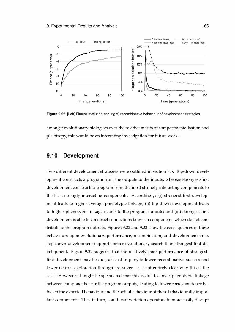
9 Experimental Results and Analysis 166
-12
-10
-8
-6
-4
-2
0
0 20 40 60 80 100
Time (generations)
Fitn
ess
(out
put e
rror
)
top-down strongest-first
0%
4%
8%
12%
16%
20%
0 20 40 60 80 100
Time (generations)
%ag
e ne
w s
olut
ions
from
c/o
Fitter (top-down) Novel (top-down)
Fitter (strongest-f irst ) Novel (strongest-f irst )
Figure 9.22. [Left] Fitness evolution and [right] recombinative behaviour of development strategies.
amongst evolutionary biologists over the relative merits of compartmentalisation and
pleiotropy, this would be an interesting investigation for future work.
9.10 Development
Two different development strategies were outlined in section 8.5. Top-down devel-
opment constructs a program from the outputs to the inputs, whereas strongest-first
development constructs a program from the most strongly interacting components to
the least strongly interacting components. Accordingly: (i) strongest-first develop-
ment leads to higher average phenotypic linkage; (ii) top-down development leads
to higher phenotypic linkage nearer to the program outputs; and (iii) strongest-first
development is able to construct connections between components which do not con-
tribute to the program outputs. Figures 9.22 and 9.23 show the consequences of these
behaviours upon evolutionary performance, recombination, and development time.
Top-down development supports better evolutionary search than strongest-first de-
velopment. Figure 9.22 suggests that the relatively poor performance of strongest-
first development may be due, at least in part, to lower recombinative success and
lower neutral exploration through crossover. It is not entirely clear why this is the
case. However, it might be speculated that this is due to lower phenotypic linkage
between components near the program outputs; leading to lower correspondence be-
tween the expected behaviour and the actual behaviour of these behaviourally impor-
tant components. This, in turn, could lead variation operators to more easily disrupt
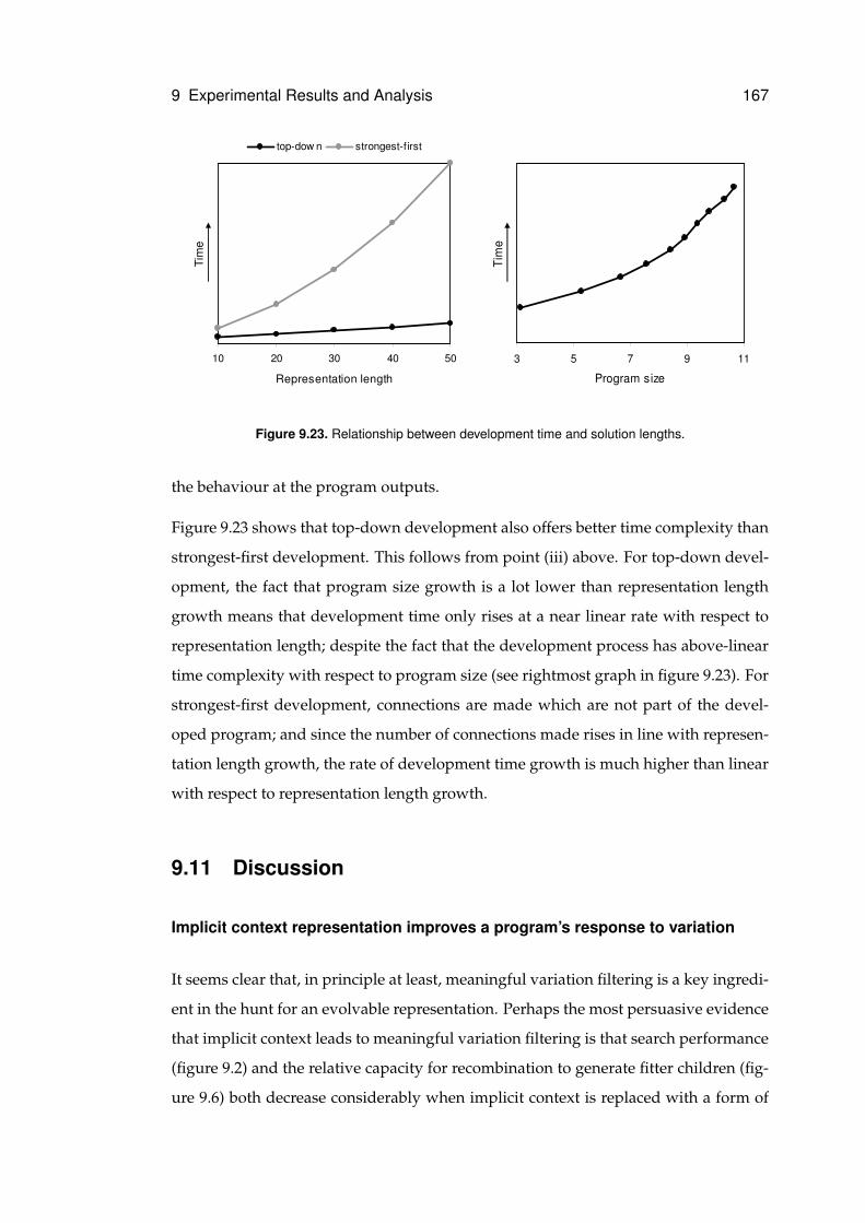
9 Experimental Results and Analysis 167
10 20 30 40 50
Representation length
Tim
e
top-dow n strongest-f irst
3 5 7 9 11
Program size
Tim
e
Figure 9.23. Relationship between development time and solution lengths.
the behaviour at the program outputs.
Figure 9.23 shows that top-down development also offers better time complexity than
strongest-first development. This follows from point (iii) above. For top-down devel-
opment, the fact that program size growth is a lot lower than representation length
growth means that development time only rises at a near linear rate with respect to
representation length; despite the fact that the development process has above-linear
time complexity with respect to program size (see rightmost graph in figure 9.23). For
strongest-first development, connections are made which are not part of the devel-
oped program; and since the number of connections made rises in line with represen-
tation length growth, the rate of development time growth is much higher than linear
with respect to representation length growth.
9.11 Discussion
Implicit context representation improves a program’s response to variation
It seems clear that, in principle at least, meaningful variation filtering is a key ingredi-
ent in the hunt for an evolvable representation. Perhaps the most persuasive evidence
that implicit context leads to meaningful variation filtering is that search performance
(figure 9.2) and the relative capacity for recombination to generate fitter children (fig-
ure 9.6) both decrease considerably when implicit context is replaced with a form of
9 Experimental Results and Analysis 168
indirect context. Hence, it follows that these beneficial behaviours are a consequence
of program components choosing their interactions according to behavioural descrip-
tions of other components rather than arbitrary patterns. To a lesser extent, this argu-
ment is also supported by performance comparison between enzyme GP and carte-
sian GP (section 9.2); although this comparison is made unreliable by the many other
differences between the two methods.
The argument that implicit context representations react in a meaningful way to change
is also supported by the recombinative behaviours outlined in section 9.4.3 which
occur as a result of the addition and removal of components. For each of these be-
haviours — subsumption, insertion, and removal — the child program ‘attempts’ to
preserve the behaviours of the parent despite changes to the program’s representation:
yet still allows change to occur. Nevertheless, there has been no quantitative study of
how often, and how effectively, these behaviours occur during program evolution;
and whilst they are seen to occur frequently, they are rarely as pure as in these exam-
ples. Furthermore, many of the behaviours which are seen during evolution do not
have such evidently beneficial characteristics. Therefore, whilst implicit context does
lead to improved variation filtering behaviours when compared to indirect context, it
seems fair to contend that this does not happen for all variation events. However, this
is generally the nature of evolutionary search.
Implicit context preserves the meaning of recombined program fragments
This is an extension to the previous point. As well as improving the capacity for a
representation to receive new components, implicit context also improves the likeli-
hood of components maintaining their meaning when transferred between programs;
and hence the capacity for a population to carry out co-operative evolution. This fol-
lows from the observation that recombination between pairs of existing representa-
tions leads to better evolutionary performance than headless chicken recombination
between existing representations and randomly constructed representations (figure
9.5). Presumably this performance advantage is due to relatively fit program frag-
ments being transferred between existing representations. Nevertheless, whilst there
is a significant difference between the performance of recombination and headless
chicken recombination, the performance of headless chicken recombination is still rel-
9 Experimental Results and Analysis 169
atively high. That a macro-mutation operator can apparently carry out useful search
supports the notion that implicit context representation improves response to varia-
tion. However, it also gives some concern that response to variation is dominant over
transfer of information in generating recombinative performance. Consequently, in
future work it might be interesting to take a closer look at how well information is
transferred between programs and whether there are mechanisms which might im-
prove the fidelity of information transfer. Genetic linkage reinforcement may be one
such mechanism; since interacting groups of components are more likely to be trans-
ferred as a unit if they are located proximal in the representation. Without genetic
linkage between components, there is some danger that transfer operations are more
likely to transfer a group of small, non-interacting, program fragments which may
either lose their behaviours or disrupt multiple sub-structures within the recipient
program. Whilst some authors [e.g. Keijzer et al., 2001] believe that it is beneficial
to change a program at multiple locations during recombination owing to increased
search potential, it also seems that this sort of operation is more likely to disrupt the
evolved behaviour of the program and lead to inviable offspring.
Functionality is a meaningful implementation of implicit context
This follows from the previous two points which show that functionality leads to
the kinds of behaviours that would be expected from a meaningful implementation
of implicit context. However, it appears that functionality is only meaningful when
its derivation reflects an appropriate balance between a component’s activity and its
binding sites (figure 9.3). Otherwise, functionality fails to capture a sufficient descrip-
tion of a component’s behaviour: either by not sufficiently describing how a compo-
nent interacts with other components, or by not sufficiently describing the compo-
nents it interacts with.
Despite its ability to describe implicit context, and the ease with which it can be calcu-
lated, functionality is not an ideal implementation of implicit context. Functionality is
limited to describing contexts in terms of a functional profile. It can not describe the
ordering or interactions between the functions in this profile. Whilst this is evidently
sufficient to describe solutions to the problems used in this chapter, it apparently
struggles to describe the kind of structural reuse seen in solutions to parity problems
9 Experimental Results and Analysis 170
(section 9.2), and it is conceivable that it is not sufficient to describe all types of struc-
ture. Consequently, an important future avenue of research would be to investigate
the applicability of functionality and, if necessary, consider other implementations of
implicit context.
Enzyme GP does not suffer from bloat
Whilst, in some circumstances, enzyme GP structures experience a degree of growth;
enzyme GP does not experience conventional GP bloating behaviour (figure 9.9). Re-
call from section 6.4 that there are a number of hypothesised causes of bloat within
tree-based GP: replication accuracy, removal bias, search space bias, and operator bias.
The replication accuracy theory contends that bloat is needed to protect programs
from the disruptive effects of recombination. It seems that whilst the recombination
operators of enzyme GP do not always carry out meaningful behaviour, TR recombi-
nation in enzyme GP is less disruptive than sub-tree crossover in tree-based GP. Partly
this is a result of variation filtering at the representation level. However, disruption
is also reduced by the decoupling between transfer and remove operations. Whereas
in conventional GP, one group of components always replace another; in enzyme GP
transfer does not physically replace components, and remove operations operate in-
dependently to transfer operations. Furthermore, as with linear GP (see section 7.4.1),
non-coding components within enzyme GP representations are able to provide a struc-
tural protection role which can, in principle, increase reproductive fidelity without the
need for the kind of global protection behaviour provided by bloating in tree-based
GP.
Removal bias can still be caused by the disparity between the success rate of transfer
and remove operators; but does not have the potential to drive bloat at anything like
the levels seen in tree-based GP. Search space bias is a property of the problem domain
rather than the search process, so presumably is still a factor in enzyme GP. There is no
operator imbalance in enzyme GP, since recombination — at least mechanistically —
has a size neutral effect. In summary, it seems that the lack of bloat in enzyme GP can
in part be explained by a lessening of the behaviours hypothesised to cause bloat in
conventional GP. However, it seems that the remaining behaviours, particularly search
space bias, should have the capacity to drive a certain amount of size growth: yet this
9 Experimental Results and Analysis 171
growth is not seen in practice.
Program size is decoupled from representation length
This occurs because components present in the representation need not be expressed
in the program. However, the representation length does place an upper limit upon
the program size, even after component reuse has been taken into account. The ad-
vantage of this decoupling is that program size evolution is not directly linked to the
action of the recombination operators and is therefore free to vary within the upper
bound set by the representation length. In practice it appears that evolution is biased
towards searching smaller program sizes: which, from a practical viewpoint, is ad-
vantageous since it leads to small, efficient solutions. It also helps to explain why rep-
resentation length does not bloat, since there is little search pressure towards higher
upper limits on program size.
There appear to be two reasons for this behaviour (section 9.7.2). First, functionalities
with a disproportionately high degree of input terminal activities are over-represented
in functionality space; giving functionality space an implicit bias towards short solu-
tions. This bias is particularly apparent when the activity set contains many input
activities and few functional activities (figure 9.19). Nevertheless, the bias only ap-
plies to random functionalities; and consequently dissipates as functionalities become
non-random during the course of evolution. Second, small programs presumably
have higher replication fidelity since they have less internal connections to be dis-
rupted when exposed to variation operators and, having shorter defining component
sequences, are more likely to be propagated during transfer operations.
In part, the trend towards smaller program size compensates for the higher time com-
plexity resulting from the development process (figure 9.23). It also leads to lower
space complexity. However, there is some danger that enzyme GP will find it harder
to solve problems with large solutions; particularly if sub-optimal solutions are short.
Some useful directions for further research will be to look at ways of removing func-
tionality bias, possibly by selecting more representative initial generation functionali-
ties, and ways of reducing the complexity of development. Perhaps the most obvious
way of reducing complexity would be to allow recurrent solutions; since most of the
development time is involved with preventing recurrency.
9 Experimental Results and Analysis 172
Redundancy improves the performance of evolutionary search
This follows from the observation that when redundant components are removed
from program representations following development, evolutionary search is substan-
tially impaired (figure 9.13). The beneficial effect of non-coding components could
either be due to a structural or functional role. Although a structural role can not
be discounted, it seems relatively difficult for non-coding components to carry out
a structural protection role in enzyme GP given that (i) there is little genetic linkage
between interacting components, and therefore little scope for the construction of lin-
ear sequences of non-coding components between coding sequences; (ii) non-coding
components do not necessarily remain non-coding following transfer, and therefore
do not substantially decrease recombinative disruption; and (iii) there is relatively lit-
tle scope for the construction of syntactic introns. However, there are good reasons
to believe that redundancy provides a beneficial effect through its functional role.
Considering that program size tends towards small solutions, it would be easy for
a population to lose functional diversity if it were not for the substantial proportion of
non-coding components found within representations. Furthermore, it seems that this
redundancy must be organised in the form of a subsumption hierarchy (section 9.4.3);
where the components at the top of the hierarchy may play a key role in enabling
back-tracking behaviours in response to disruptive variation events. This apparently
beneficial functional role of redundancy also agrees with the findings of much of the
research reviewed in section 7.4.3.
Lamarckian reinforcement learning can significantly improve performance
A reinforcement learning rate of 1% of the difference between a binding site and the
shape of its bound component leads to a 50% improvement in success rate and a signif-
icant reduction in the average number of generations required to evolve a two-bit mul-
tiplier (figure 9.17). Presumably this is due to the stabilising effect that reinforcement
learning has upon the building blocks of evolving programs. Given that interactions
are reinforced following each variation event, reinforcement learning will give most
stability to those building blocks which have remained in the same program through-
out a number of variation events or have passed through a number of programs via
transfer operations. Therefore, reinforcement learning implicitly strengthens those
9 Experimental Results and Analysis 173
building blocks which have a high effective fitness; and in effect increases their effec-
tive fitness over time by making them easier to propagate between programs. The
benefits of Lamarckian reinforcement learning within enzyme GP mirrors its benefits
within other GP systems [Teller, 1999, Downing, 2001]. The trade-off between explo-
ration and exploitation in choosing an appropriate learning rate in enzyme GP also
mirrors the balance between insufficient learning and over-learning when choosing a
learning rate for the neural network back-propagation algorithm.
10 Summary and Conclusions
This chapter summarises the work reported in this thesis and the rationale behind it;
presents conclusions; discusses limitations of the experimental method; and specu-
lates about further work.
10.1 Rationale and Work Done
This thesis began with the goal of mining biological knowledge to improve the be-
haviour and performance of genetic programming. Biology has served as an inspi-
ration to computer science throughout its history. Many fields of modern computer
science, such as machine vision, robotics, and neural networks, place an implicit em-
phasis upon the mimicry of biological systems in both their goals and their methods.
Indeed, biology possesses many of the attributes which many people would one day
like to see in computer systems, including: fault tolerance, self repair, autonomous be-
haviour, self-replication, intelligence, learning, reconfigurability and environmental
interaction. Yet, according to Charles Darwin’s theory of evolution, all these attributes
came about through an iterative process of selection acting upon random change to
some initially very simple organism — and herein lies the motivation behind evolu-
tionary computation.
Nevertheless, both our understanding of biology and our understanding of change
within non-biological systems points to the realisation that a complex artifact can only
be evolved if the artifact is internally organised in a suitable way. For example, it is
very difficult to derive a complex software system from a basic software system if the
basic software system does not have a meaningful architecture or is not written in leg-
174
10 Summary and Conclusions 175
ible code — and this is true even if the changes are being made by an experienced and
intelligent programmer. Within biological systems, genetic change is essentially ran-
dom: yet biological systems are still considered to be highly evolvable. This is because
biological systems are internally organised in a way that, to an extent, prevents inap-
propriate change and promotes meaningful change. The sources of evolvability within
biological systems exist at many levels and include: redundancy, compartmentali-
sation, exploratory mechanisms, and epigenetic and ecological processes. However,
perhaps one of the most important sources of evolvability in biology is that behaviour
emerges bottom-up from interactions between biological components which implicitly
know what they want to do and what they want to do it to. This characteristic has
been termed ‘implicit context’ within this thesis.
By comparison, most genetic programming systems use what could be termed ‘ex-
plicit context’ representations: where the interactions between components are deter-
mined explicitly by their position within the representation. However, such position-
ally dependent representations have important limitations: (i) a component loses its
context, and hence changes its behaviour, if its relative position is changed; and (ii)
particular positions can have different meanings within different programs. This im-
plies that recombination operators, which move components between programs and
typically change their position, rarely preserve the behaviour of the components they
recombine; with the consequence that co-operative evolution — a conceptually power-
ful form of evolution — can not easily occur within genetic programming populations.
A number of non-standard GP systems [Poli, 1997, Luke et al., 1999, Miller and Thom-
son, 2000, Oltean and Dumitrescu, 2002] use an alternative form of representation
which, in this thesis, is termed ‘indirect context’. In an indirect context representation,
each component is assigned a reference and each component specifies its interactions
with other components according to these references. Explicit context can be seen as a
special case of indirect context in which a component’s reference is its position within
a program representation and in which components can only occupy positions which
are referred to by other components. In an indirect context representation, by compar-
ison, components may be assigned references that are not referred to by other compo-
nents within the representation. Consequently, these components are not used within
the program described by the representation but can be used to support modes of
10 Summary and Conclusions 176
evolution believed to be significant sources of evolvability in biological systems: such
as neutral evolution and analogues of evolution be gene duplication. It is also possi-
ble for a component to be referred to by more than one other component, a condition
comparable to pleiotropy in biological systems. Importantly, a component’s reference
need not be related to its position within the representation, and hence components
can be moved within a representation without changing their behaviour. However,
particular references can still have different meanings within different programs: and
consequently indirect context does not prevent the loss of a component’s meaning
following recombination.
The work reported in this thesis concerns the development of an implicit context rep-
resentation for genetic programming. The potential benefits of implicit context for
evolutionary computation are very significant. Within biological systems, the be-
haviour of a biological component — both what it does and what it interacts with — is
determined solely by its chemical constitution and physical shape: both of which are
a consequence of its genetic definition. Loosely speaking, if during recombination a
biological component’s genetic definition is moved from the genome of one organism
to the genome of another and the component becomes expressed, it will implicitly at-
tempt to carry out the same behaviour in this new organism that it did in the previous
organism i.e. its meaning will be preserved following recombination. This happens
because biological components interact with other biological components according to
recognition of one another’s shape, which describes their behaviour, rather than one
another’s genomic position or other arbitrary reference. For example, the shape of an
enzyme’s binding site is complementary to that of its substrate; so the enzyme is ef-
fectively describing (in part) the behaviour of the component it would like to interact
with.
The notion of an implicit context representation for genetic programming is based
upon this biological concept of implicit context. Rather than program components
specifying their context via explicit position or indirect reference, in an implicit con-
text representation components specify their interactions in terms of the behaviour
of the components they would like to interact with. However, in order for this to be
possible, components must be able to interrogate other components to determine their
behaviour. Assume for the moment that there is a perfect mechanism whereby compo-
10 Summary and Conclusions 177
nents can determine the behaviour of others. Following recombination, a component
would be able to inspect other components and determine whether or not there are
any components it should interact with in order to achieve its pre-defined behaviour.
Note that there is no requirement for a component to become involved in a program
if there are no suitable interactions. In this situation the component would become re-
cessive. However, any behaviour which a component does carry out will be consistent
across programs.
Variation operators can alter a program representation in four different ways. They
can add components, remove components, re-order components, or change (mutate)
the behaviour of components: either by changing how they should interact with other
components (their function) or by changing which components they should interact
with. The use of implicit context leads to a phenomenon which is termed ‘variation
filtering’ within this thesis; whereby particular variation events can be wholly or par-
tially ignored. For example, if a component is added to a program representation,
then it will only affect the program’s outputs if it interacts with existing components
that are expressed in the program i.e. only if it fits into the existing contexts declared
by the program. If an expressed program component is removed from a program
representation, then it might be possible for the other expressed components to com-
pensate for its absence by interacting with a previously recessive component with a
similar behaviour. This could also happen if an expressed component lost its previous
behaviour as a result of a mutation event; or conversely a mutation event might cause
a previously recessive component to offer a better match to an existing component’s
interaction preference than a currently expressed component. In effect, there is a ten-
dency for variation events to be ignored or partially compensated for if they cause
change which does not fit the contexts currently declared by the program. This, in
turn, promotes gradual change in program behaviour: something which is conceptu-
ally desirable from the perspective of evolvability.
Enzyme genetic programming is a form of genetic programming based upon an imple-
mentation of implicit context representation. In enzyme GP, a program is a collection
of inter-connected functions, program inputs, and program outputs. A program is
represented by a linear array of program components, each of which has: an activity;
a behavioural description; and — if it processes input — a set of input preferences,
10 Summary and Conclusions 178
which describe the behaviour of the components whose outputs it would most like to
receive inputs from. A program representation is mapped into a program via a de-
velopment process which attempts to connect the inputs of every component to the
outputs of those components which most closely match their input preferences.
Unlike in biology, it would be insufficiently precise to describe a program component
by its activity alone, since both within a single program and within a population of
programs there will be many program components with the same activity but with
different roles. To overcome this problem, a program component, in enzyme GP, is
described by both its own activity and the activities of the components which develop
below its inputs. However, the exact components which develop below a component’s
inputs can not be known until after the development process is complete. Conse-
quently, enzyme GP must describe a component’s behaviour in terms of its expected
inputs; those components which would be connected to its inputs if its behavioural
preferences were matched precisely during development. This description is called a
functionality and, in effect, declares a component’s behaviour as an expected activity
profile, weighted by depth, of the components that occur in the program fragment of
which it is the root.
10.2 Conclusions
Enzyme genetic programming has been applied to a range of discrete symbolic re-
gression problems. Analysis of the performance and behaviour of the evolutionary
process has led to a number of conclusions.
Implicit context leads to meaningful variation filtering
Meaningful variation filtering is defined as the capacity for an evolutionary system to
filter out inappropriate change caused by the action of variation operators. Theoreti-
cally (see above), the use of implicit context representation should allow an evolution-
ary system to carry out meaningful variation filtering. This is supported by a signif-
icant amount of experimental evidence indicating that enzyme genetic programming
does carry out meaningful variation filtering.
10 Summary and Conclusions 179
Meaningful variation filtering promotes meaningful recombination
The main experimental evidence that enzyme GP carries out meaningful variation fil-
tering lies in the ability of enzyme GP to carry out meaningful recombination. When
compared to indirect context, enzyme GP’s implicit context representation leads to
a substantial improvement in recombinative performance: both in the capacity for a
program representation to receive components transferred from another program rep-
resentation, and in its capacity to preserve the meaning of the transferred components.
These quantitative results are supported by the identification of context-preserving
behaviours during qualitative analysis of the effect of recombination upon individual
programs.
Meaningful variation filtering is supported by redundancy
It has been hypothesised that the redundant portions of implicit context program rep-
resentations are organised into a subsumption hierarchy; and that this subsumption
hierarchy supports meaningful variation filtering by absorbing inappropriate change
and saving subsumed program components in case they are needed for back-tracking.
The utility of this structure can be seen in the observation that the non-coding por-
tion of representations grows in response to the addition of components; filtering out
components which do not fit into the contexts defined by programs. Evolutionary
performance is substantially degraded when redundancy is stripped from program
representations following program development. This supports the views of other
researchers that functional redundancy is an important source of evolvability within
evolutionary representations [e.g. Smith and Goldberg, 1992, Dasgupta and McGre-
gor, 1993, Haynes, 1996, Levenick, 1999, Yu and Miller, 2002].
Meaningful variation filtering gradualises change
Output terminal components have an important role in program development for they
uniquely determine the program’s output context and therefore which components
will contribute to the program behaviour following development. Furthermore, by
attempting to make the same input connections, they attempt to implement the same
output behaviour irrespective of which components are actually present within the
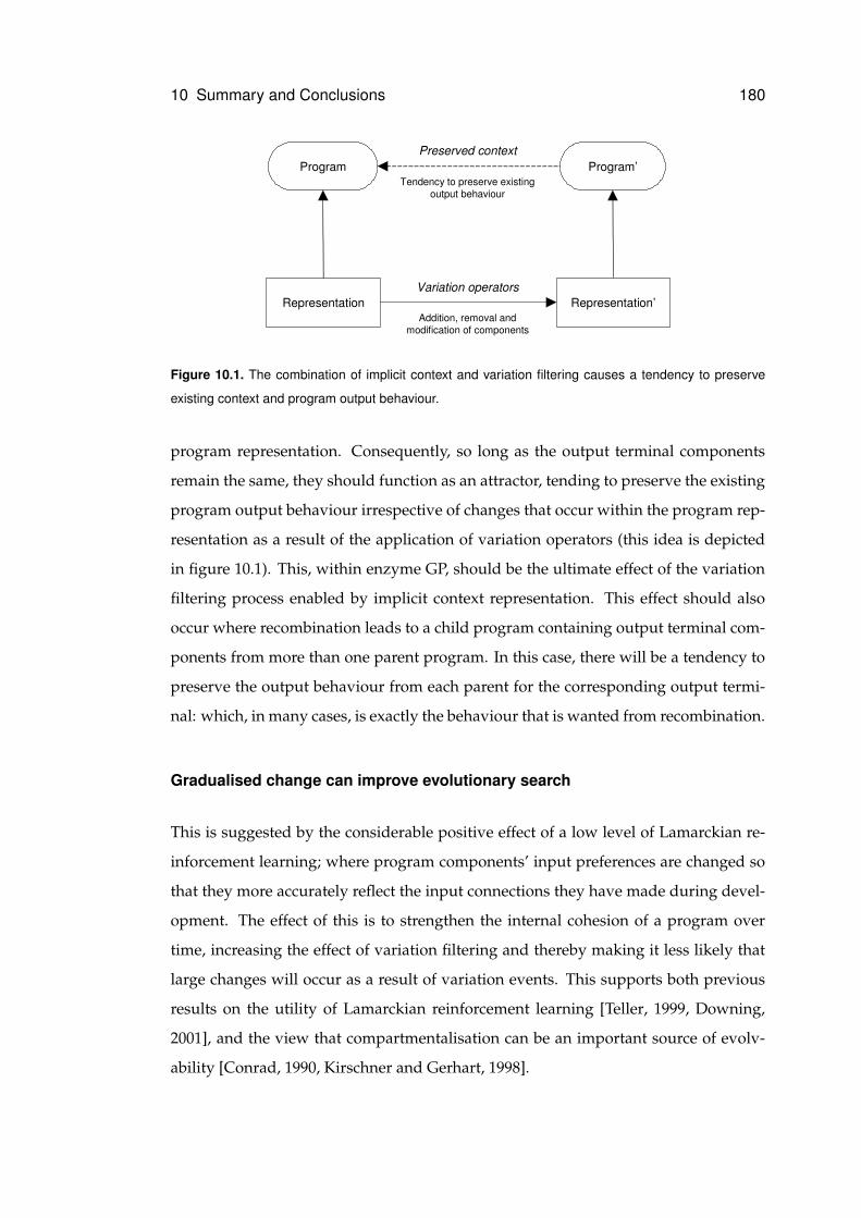
10 Summary and Conclusions 180
Representation
Program
Representation’
Program’
Variation operators
Preserved context
Addition, removal and modification of components
Tendency to preserve existing output behaviour
Figure 10.1. The combination of implicit context and variation filtering causes a tendency to preserve
existing context and program output behaviour.
program representation. Consequently, so long as the output terminal components
remain the same, they should function as an attractor, tending to preserve the existing
program output behaviour irrespective of changes that occur within the program rep-
resentation as a result of the application of variation operators (this idea is depicted
in figure 10.1). This, within enzyme GP, should be the ultimate effect of the variation
filtering process enabled by implicit context representation. This effect should also
occur where recombination leads to a child program containing output terminal com-
ponents from more than one parent program. In this case, there will be a tendency to
preserve the output behaviour from each parent for the corresponding output termi-
nal: which, in many cases, is exactly the behaviour that is wanted from recombination.
Gradualised change can improve evolutionary search
This is suggested by the considerable positive effect of a low level of Lamarckian re-
inforcement learning; where program components’ input preferences are changed so
that they more accurately reflect the input connections they have made during devel-
opment. The effect of this is to strengthen the internal cohesion of a program over
time, increasing the effect of variation filtering and thereby making it less likely that
large changes will occur as a result of variation events. This supports both previous
results on the utility of Lamarckian reinforcement learning [Teller, 1999, Downing,
2001], and the view that compartmentalisation can be an important source of evolv-
ability [Conrad, 1990, Kirschner and Gerhart, 1998].
10 Summary and Conclusions 181
Implicit context leads to improved size evolution characteristics
It is difficult to make general conclusions regarding the effect of implicit context rep-
resentation upon the evolution of program size, since program size within enzyme
GP appears to be significantly affected by inherent biases within the functionality im-
plementation of implicit context. However, it can be speculatively suggested that GP
with implicit context representation should suffer significantly less from bloat than GP
with explicit context representation, given that: (i) recombination is less disruptive; (ii)
the recombination mechanism does not promote the development of protective syn-
tactic introns; (iii) the effect of removal bias is far smaller; and (iv) program size is
decoupled from representation length. This argument is somewhat supported by the
observation that there is little or no bloat in enzyme GP. It has also been hypothesised
that small programs are better replicators than large programs, since they have less
internal connections and are therefore less likely to be disrupted by variation events.
This is also supported by the tendency towards the evolution of small programs in en-
zyme GP. However, there is some concern that this might make it harder to solve prob-
lems which have large optimal solutions and relatively short sub-optimal solutions —
although this concern is somewhat allayed by the diversity preservation mechanism
that is inherent in implicit context representations.
These conclusions support the hypothesis that models of biological representations
can be used to represent computer programs and other artificial executable structures
within genetic programming, thereby improving the evolvability of these structures.
10.3 Limitations of This Study
Whilst considerable effort has been made to verify these conclusions through both
experimental investigation and theoretical understanding, there are limitations of the
experimental method which might reduce their generality. The most significant limita-
tion is that the performance of enzyme genetic programming has not been vigorously
analysed upon a wider class of problems; and whilst discrete symbolic regression was
chosen for its relative difficulty with regard to recombination, it can not be representa-
tive of all other problem domains. Partly this limitation reflects a need to generalise the
10 Summary and Conclusions 182
functionality implementation of implicit context to handle so-called ephemeral ran-
dom constants and structural behaviours in addition to functional behaviours. Sug-
gestions as to how this might be done are given in the further work section. Fur-
thermore, there has been little direct comparison between the performance of enzyme
genetic programming and conventional genetic programming. This is due both to
the lack of existing results applying conventional GP to Boolean regression problems,
and to the difficulty of direct performance comparison caused by the use of a non-
standard evolutionary framework within enzyme GP. However, it is assumed that
explicit context representations have worse performance than indirect context repre-
sentations upon recombinative search (for reasons given elsewhere in this thesis); and
that therefore the performance of explicit and implicit context are being compared by
transitivity. Nevertheless, it is hoped that these limitations will be addressed in future
research.
10.4 Further Work
Section 9.7.2 discussed how biases within functionality space may lead to size and
structural biases during search. An important avenue for future work will be to look
into ways of removing this bias. Bias can be reduced by warping functionality space
so that changes within over-represented regions have less influence upon the evolu-
tionary process. However, early work concerned with variable dimension lengths had
led to little success. Perhaps a more effective approach, in the short term, will be to
look at ways of biasing the initialisation and mutation mechanisms in order to coun-
teract the biases in fuctionality space; although a more long term strategy should be to
look at alternative reference spaces which do not have the same kinds of biases which
are seen in functionality space.
Perhaps a more important short term goal should be to reduce the time complexity
of development. The most obvious way of doing this would be to remove the non-
recurrency constraint during development. Without this constraint, development will
simply be a process of comparing the input preferences and behavioural descriptions
of each pair of components; a process which will have far less complexity than main-
taining and interrogating connection information at each node in order to determine
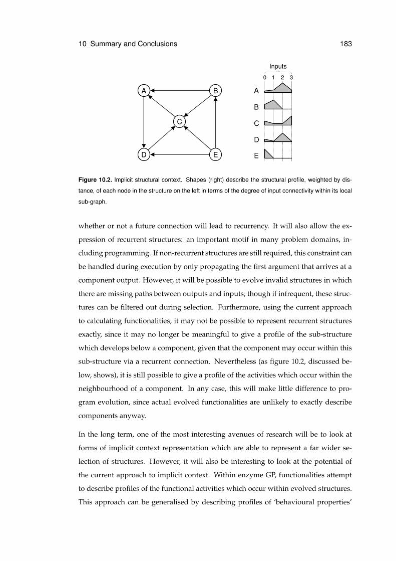
10 Summary and Conclusions 183
A B
D E
C
A
B
C
D
E
0 1 2 3
Inputs
Figure 10.2. Implicit structural context. Shapes (right) describe the structural profile, weighted by dis-
tance, of each node in the structure on the left in terms of the degree of input connectivity within its local
sub-graph.
whether or not a future connection will lead to recurrency. It will also allow the ex-
pression of recurrent structures: an important motif in many problem domains, in-
cluding programming. If non-recurrent structures are still required, this constraint can
be handled during execution by only propagating the first argument that arrives at a
component output. However, it will be possible to evolve invalid structures in which
there are missing paths between outputs and inputs; though if infrequent, these struc-
tures can be filtered out during selection. Furthermore, using the current approach
to calculating functionalities, it may not be possible to represent recurrent structures
exactly, since it may no longer be meaningful to give a profile of the sub-structure
which develops below a component, given that the component may occur within this
sub-structure via a recurrent connection. Nevertheless (as figure 10.2, discussed be-
low, shows), it is still possible to give a profile of the activities which occur within the
neighbourhood of a component. In any case, this will make little difference to pro-
gram evolution, since actual evolved functionalities are unlikely to exactly describe
components anyway.
In the long term, one of the most interesting avenues of research will be to look at
forms of implicit context representation which are able to represent a far wider se-
lection of structures. However, it will also be interesting to look at the potential of
the current approach to implicit context. Within enzyme GP, functionalities attempt
to describe profiles of the functional activities which occur within evolved structures.
This approach can be generalised by describing profiles of ‘behavioural properties’
10 Summary and Conclusions 184
within structures, which could include both functional and non-functional properties
of their components. Figure 10.2, for example, shows how descriptive shapes can
be used to represent an arbitrary digraph. Rather than describing the functions of
the nodes within the structure, these shapes describe nodes by the number of incom-
ing connections they have from other nodes. In theory, this approach could be used
for any kind of structure; although in practice it would require that structures have
sufficient heterogeneity in the connectivity of their nodes and the distribution of con-
nectivity within the structure. However, as problems such as the two-bit multiplier
show, the behavioural properties (e.g. activity types) within a structure do not have to
be very diverse in order for it to be expressed and evolved by this method. Further-
more, there is no reason why a descriptive shape could not describe both functional
and non-functional properties together. For example, the behaviours of components
within digital circuits could be described by profiles of both the functional and struc-
tural properties of their expected sub-trees. There is also scope for describing con-
tinuous parameters. For example, ephemeral random constants have two functional
properties: they are a constant input source and they provide a particular value. One
functionality dimension could be used to describe the relative occurrence of constants
within a program fragment and one could could be used to describe the relative value
of the constants.
Recently, there has been some interest in using implicit context1 within manual pro-
gramming environments. In an approach described by Walker and Murphy [2000],
components analyse their call history in order to learn more about the behaviour they
are expected to provide to other components. Because of this, components are able
to request behaviour from one another via fewer function calls and fewer parame-
ters; simplifying component interaction and leading to communication along narrow,
well-defined paths. Due to cleaner interfaces and less complex connectivity, this form
of implicit context, in principle, makes it easier for components to be re-used within
other programs. Whilst only partially related to the idea of implicit context introduced
in this thesis, this idea of a component learning its own context could be used within
an EC implicit context representation. Lamarckian reinforcement learning is an exist-
ing mechanism whereby context learning can take place in the functionality model of
implicit context. However, this form of learning is currently carried out at a program
1This use of the term implicit context, whilst related, was coined independently.
10 Summary and Conclusions 185
level and can only learn simple information about those activities which have dimen-
sions within functionality space. A more complex form of learnt implicit context can
be imagined in which a program consists of software agents which can flexibly learn
about their environment and preserve this information when transferred between pro-
grams; gradually building up knowledge about the space of possible component in-
teractions and their expected behaviour within this space. At the start of evolution,
these agents would only have a general idea of the role they should fulfill — mak-
ing behavioural exploration easy — but, during the course of evolution, they would
become more specialised — improving behavioural exploitation.
Such behaviourally complex forms of implicit context representation could also be
used within software engineering environments. Rather than programmers scripting
the interactions between program components; implicit context would allow them
to focus on writing components. When these components are placed in a program
together, the program behaviour would emerge from implicit interactions between
components. This would amount to applying biological principles of organisation to
the realm of human design. However, this vision is currently rather far-fetched (and
perhaps even impractical!). Perhaps a more productive goal in the meantime would be
to apply more of the principles of biological organisation to the development of evolu-
tionary computation representations. Thus far, in this thesis, this approach has led to
the development of a representation modelled upon the interactions within metabolic
pathways. It seems conceivable that this model could be extended to include the in-
teractions between metabolic pathways and signalling and gene expression pathways.
Gene expression pathways, in biology, are evidently the source of many of the more
complex behaviours seen within biological systems. Signalling pathways are the pre-
dominant source of distributed processing within biological systems; and distributed
processing appears to be an important factor both behaviourally and as a source of
evolvability within biological representations. Certainly it is conceivable that the en-
zyme GP model could be extended to allow regulation of component expression by
currently expressed components (a behaviour which could be particularly useful for
solving dynamic problems) and to allow communication between ‘cellular’ groups of
components (which might themselves result from differential component expression).
However, whilst making the system far more expressive, this will also make it harder
to interpret by a human.
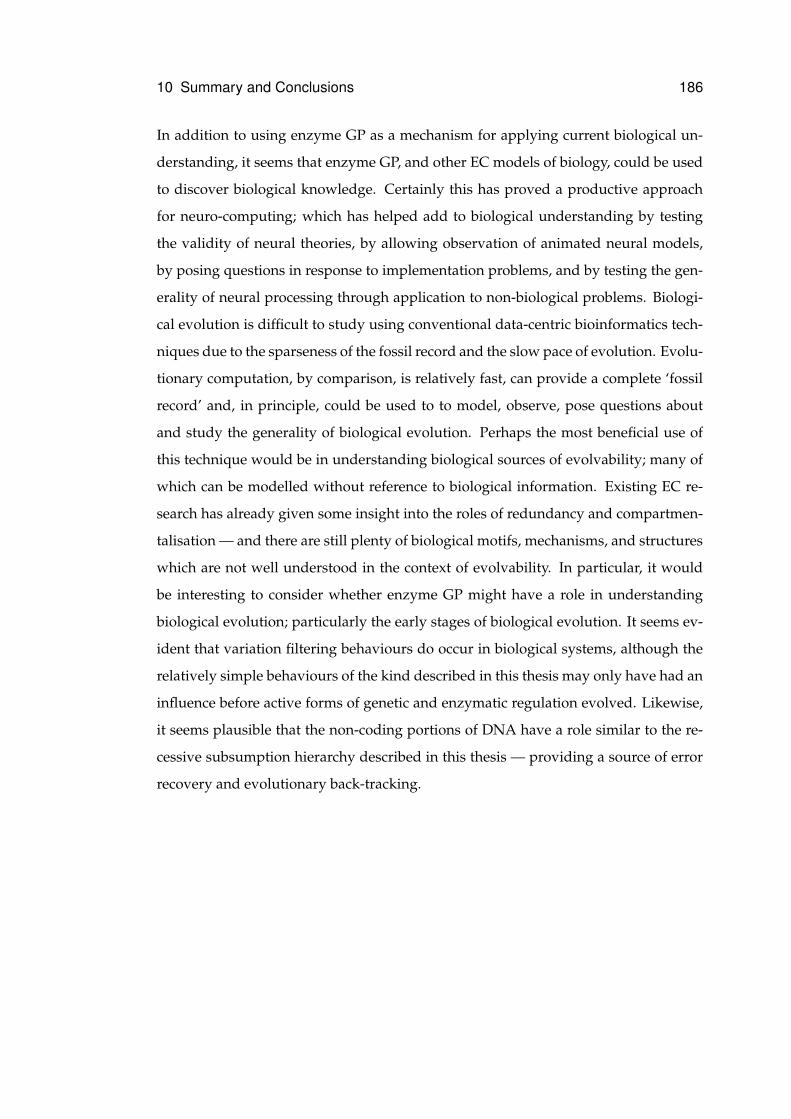
10 Summary and Conclusions 186
In addition to using enzyme GP as a mechanism for applying current biological un-
derstanding, it seems that enzyme GP, and other EC models of biology, could be used
to discover biological knowledge. Certainly this has proved a productive approach
for neuro-computing; which has helped add to biological understanding by testing
the validity of neural theories, by allowing observation of animated neural models,
by posing questions in response to implementation problems, and by testing the gen-
erality of neural processing through application to non-biological problems. Biologi-
cal evolution is difficult to study using conventional data-centric bioinformatics tech-
niques due to the sparseness of the fossil record and the slow pace of evolution. Evolu-
tionary computation, by comparison, is relatively fast, can provide a complete ‘fossil
record’ and, in principle, could be used to to model, observe, pose questions about
and study the generality of biological evolution. Perhaps the most beneficial use of
this technique would be in understanding biological sources of evolvability; many of
which can be modelled without reference to biological information. Existing EC re-
search has already given some insight into the roles of redundancy and compartmen-
talisation — and there are still plenty of biological motifs, mechanisms, and structures
which are not well understood in the context of evolvability. In particular, it would
be interesting to consider whether enzyme GP might have a role in understanding
biological evolution; particularly the early stages of biological evolution. It seems ev-
ident that variation filtering behaviours do occur in biological systems, although the
relatively simple behaviours of the kind described in this thesis may only have had an
influence before active forms of genetic and enzymatic regulation evolved. Likewise,
it seems plausible that the non-coding portions of DNA have a role similar to the re-
cessive subsumption hierarchy described in this thesis — providing a source of error
recovery and evolutionary back-tracking.
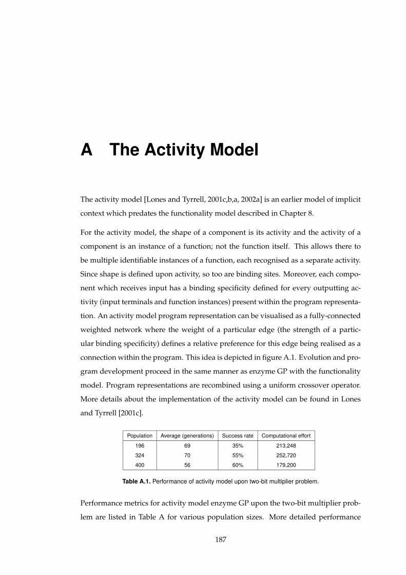
A The Activity Model
The activity model [Lones and Tyrrell, 2001c,b,a, 2002a] is an earlier model of implicit
context which predates the functionality model described in Chapter 8.
For the activity model, the shape of a component is its activity and the activity of a
component is an instance of a function; not the function itself. This allows there to
be multiple identifiable instances of a function, each recognised as a separate activity.
Since shape is defined upon activity, so too are binding sites. Moreover, each compo-
nent which receives input has a binding specificity defined for every outputting ac-
tivity (input terminals and function instances) present within the program representa-
tion. An activity model program representation can be visualised as a fully-connected
weighted network where the weight of a particular edge (the strength of a partic-
ular binding specificity) defines a relative preference for this edge being realised as a
connection within the program. This idea is depicted in figure A.1. Evolution and pro-
gram development proceed in the same manner as enzyme GP with the functionality
model. Program representations are recombined using a uniform crossover operator.
More details about the implementation of the activity model can be found in Lones
and Tyrrell [2001c].
Population Average (generations) Success rate Computational effort
196 69 35% 213,248
324 70 55% 252,720
400 56 60% 179,200
Table A.1. Performance of activity model upon two-bit multiplier problem.
Performance metrics for activity model enzyme GP upon the two-bit multiplier prob-
lem are listed in Table A for various population sizes. More detailed performance
187
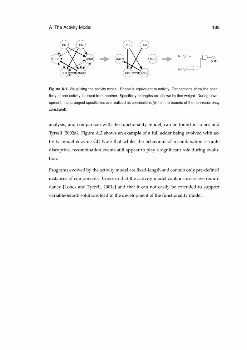
A The Activity Model 188
IN1 IN2
OR1 AND2
OUT1 AND1IN1
IN2
OUT1
IN1 IN2
OR1 AND2
OUT1 AND1
Figure A.1. Visualising the activity model. Shape is equivalent to activity. Connections show the speci-
ficity of one activity for input from another. Specificity strengths are shown by line weight. During devel-
opment, the strongest specificities are realised as connections (within the bounds of the non-recurrency
constraint).
analysis, and comparison with the functionality model, can be found in Lones and
Tyrrell [2002a]. Figure A.2 shows an example of a full adder being evolved with ac-
tivity model enzyme GP. Note that whilst the behaviour of recombination is quite
disruptive, recombination events still appear to play a significant role during evolu-
tion.
Programs evolved by the activity model are fixed-length and contain only pre-defined
instances of components. Concern that the activity model contains excessive redun-
dancy [Lones and Tyrrell, 2001c] and that it can not easily be extended to support
variable-length solutions lead to the development of the functionality model.
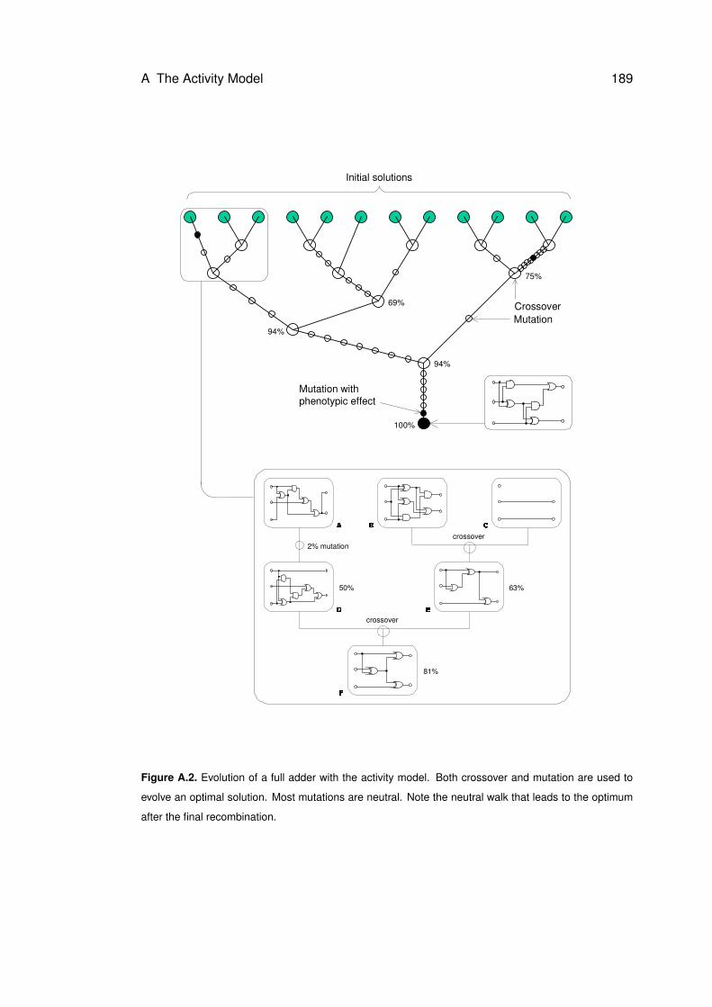
A The Activity Model 189
94%
94%
69%
75%
100%
CrossoverMutation
Mutation�with�phenotypic�effect
Initial�solutions
J K
L
M
N
O
2%�mutationcrossover
crossover
50% 63%
81%
Figure A.2. Evolution of a full adder with the activity model. Both crossover and mutation are used to
evolve an optimal solution. Most mutations are neutral. Note the neutral walk that leads to the optimum
after the final recombination.
Bibliography
L. Altenberg. The evolution of evolvability in genetic programming. In K. Kinnear, Jr, editor, Advances inGenetic Programming. MIT Press, 1994.
D. Andre and A. Teller. A study in program response and the negative effects of introns in geneticprogramming. In J. R. Koza, D. E. Goldberg, D. B. Fogel, and R. L. Riolo, editors, Proceedings of GeneticProgramming 1996: Proceedings of the First Annual Conference, pages 12–20, Stanford, USA, 1996.
P. Angeline. Genetic programming and emergent intelligence. In K. Kinnear, Jr, editor, Advances in GeneticProgramming. MIT Press, 1994.
P. Angeline. Subtree crossover: Building block engine or macromutation? In John R Koza, KalyanmoyDeb, Marco Dorigo, David B Fogel, Max Garzon, Hitoshi Iba, and Rick L Riolo, editors, Genetic Pro-gramming 1997: Proceedings of the Second Annual Conference, GP97, pages 240–248. Morgan Kaufmann,1997.
P. Angeline. Multiple interacting programs: A representation for evolving complex behaviors. Cyberneticsand Systems, 29(8):779–806, 1998a.
P. Angeline. Subtree crossover causes bloat. In Proceedings of the 1998 Conference on Genetic Programming(GP98), 1998b.
R. Muhammad Atif Azad and C. Ryan. Structural emergence with order independent representations.In E. Cantu-Paz et al., editor, Proceedings of the 2003 Genetic and Evolutionary Computation Conference,GECCO 2003, volume 2724 of Lecture Notes in Computer Science, pages 1626–1638. Springer-Verlag,2003.
J. Bagley. The Behaviour of Adaptive Systems Which Employ Genetic and Correlation Algorithms. PhD thesis,University of Michigan, 1967.
W. Banzhaf, P. Nordin, R. E. Keller, and F. D. Francone. Genetic programming: An introduction. MorganKaufmann, San Francisco, 1998.
G. Barreau. The evolutionary consequences of redundancy in natural and artificial genetic codes. PhD thesis,University of Sussex, Brighton, UK, May 2002.
G. Battail. An engineer’s view on genetic information and biological evolution. In Proceedings of theFifth International Workshop on Information Processing in Cells and Tissues, (also to appear in BioSystems),September 2003.
M. A. Bedau and N. H. Packard. Evolution of evolvability via adaptation of mutation rates. BioSystems,69:143–162, 2003.
190
BIBLIOGRAPHY 191
F. A. Bignone, R. Livi, and M. Propato. Complex evolution in genetic networks. Europhysics Letters, 40(5):497–502, December 1997.
T. Blickle and L. Thiele. Genetic programming and redundancy. In J. Hopf, editor, Genetic Algorithmswithin the Framework of Evolutionary Computation (Workshop at KI-94, Saarbrucken), pages 33–38. Max-Planck-Institut fur Informatik, 1994.
E. Boers and H. Kuiper. Biological metaphors and the design of modular neural networks. Master’sthesis, Leiden University, Department of Computer Science and Department of Experimental andTheoretical Psychology, 1992.
S. Bornholdt and T. Rohlf. Topological evolution of dynamical networks: Global criticality from localdynamics. Physical Review Letters, 84(26):6114–6117, June 2000.
S. Bornholdt and K. Sneppen. Neutral mutations and punctuated equilibrium in evolving genetic net-works. Physical Review Letters, 81(1):236–239, July 1998.
D. Bray and S. Lay. Computer simulated evolution of a network of cell-signalling molecules. BiophysicalJournal, 66:972–977, 1994.
D. Bray. Protein molecules as computational elements in living cells. Nature, 376:307–312, 1995.
T. A. Brown and A. Brown. Genomes. John Wiley and Sons, 2nd edition, 2002.
E. Chiva and P. Tarroux. Evolution of biological regulation networks under complex environmentalconstraints. Biological Cybernetics, 73:323–333, 1995.
C. Coello, A. Christiansen, and A. Hernandez-Aguirre. Use of evolutionary techniques to automate thedesign of combinational circuits. International Journal of Smart Engineering System Design, 2(4):299–314,June 2002.
E. Collingwood, D. Corne, and P. Ross. Useful diversity via multiploidy. In Proceedings of the IEEEInternational Conference on Evolutionary Computing, pages 810–813, 1996.
M. Conrad. Bootstrapping on the adaptive landscape. BioSystems, 11:167–182, 1979.
M. Conrad. The mutation-buffering concept of biomolecular structure. Journal of Bioscience, 8:669–679,1985.
M. Conrad. The geometry of evolution. BioSystems, 24:61–81, 1990.
N. Cramer. A representation for the adaptive generation of simple sequential programs. In J. Grefenstette,editor, Proceedings of the International Conference on Genetic Algorithms and their Applications, pages 183–187, 1985.
C. Darwin. On the Origin of Species by Means of Natural Selection, or the Preservation of Favoured Races in theStruggle for Life. John Murray, London, 1859.
D. Dasgupta and D. McGregor. Engineering optimizations using the structured genetic algorithm. InProceedings of the 1992 European Conference on Artificial Intelligence, ECAI-92, pages 608–609, 1992a.
D. Dasgupta and D. McGregor. Non-stationary function optimization using the structured genetic algo-rithm. In Proceedings of Parallel Problem Solving from Nature II, PPSN-2, pages 145–154, 1992b.
D. Dasgupta and D. McGregor. sga: A structured genetic algorithm. Technical Report IKBS-11-93.ps.Z,Department of Computer Science, University of Strathclyde, April 1993.
BIBLIOGRAPHY 192
R. Dawkins. The Selfish Gene. Oxford University Press, 1976.
R. Dawkins. The evolution of evolvability. In C. Langton, editor, Artificial Life: The proceedings of an in-terdisciplinary workshop on the synthesis and simulation of living systems, pages 201–220. Addison-Wesley,1989.
K. L. Downing. Reinforced genetic programming. Genetic Programming and Evolvable Machines, 2(3):259–288, 2001.
K. L. Downing. Developmental models for emergent computation. In A. Tyrrell, P. Haddow, and J. Tor-resen, editors, Proceedings of the Fifth International Conference on Evolvable Systems, ICES2003, volume2606 of Lecture Notes in Computer Science, pages 105–116. Springer-Verlag, 2003.
M. Ebner, M. Shackleton, and R. Shipman. How neutral networks influence evolvability. Complexity, 7(2):19–33, 2001.
European Bioinformatics Institute. Database of functional networks in living organisms.http://www.ebi.ac.uk/research/pfmp/, 2000.
C. Ferreira. Gene expression programming: A new adaptive algorithm for solving problems. ComplexSystems, 13(2):87–129, 2001.
M. J. Fisher, R. C. Paton, and K. Matsuno. Intracellular signalling proteins as ‘smart’ agents in paralleldistributed processes. BioSystems, 50:159–171, 1999.
L. Fogel, A. Owens, and M Walsh. Artificial intelligence through simulated evolution. Wiley, 1966.
S. Forrest and M. Mitchell. Relative building-block fitness and the building-block hypothesis. In D. Whit-ley, editor, Foundations of Genetic Programming 2. Morgan Kaufmann, 1993.
C. Forst and K. Schulten. Evolution of metabolisms: A new method for the comparison of metabolicpathways using genomics information. In Proceedings of the third annual international conference onComputational molecular biology, pages 174–181. ACM, April 1999.
F. Francone, M. Conrads, W. Banzhaf, and P. Nordin. Homologous crossover in genetic programming.In W. Banzhaf, J. Daida, A. Eiben, M. Garzon, V. Honavar, M. Jakiela, and R. Smith, editors, Proceed-ings of the 1999 Genetic and Evolutionary Computation Conference, GECCO‘99, pages 1021–1026. MorganKaufmann, 1999.
R. Friedberg. A learning machine, part I. IBM Journal of Research and Development, 2:2–13, 1958.
W. Gilbert. Why genes in pieces? Nature, 271:501, 1978.
D. E. Goldberg, K. Deb, H. Kargupta, and H. George. Rapid accurate optimization of difficult problemsusing fast messy genetic algorithms. In S. Forrest, editor, Proceedings of The Fifth International ConferenceOn Genetic Algorithms. Morgan Kaufmann, 1993.
D. E. Goldberg. Genetic Algorithms in Search, Optimisation and Machine Learning. Addison-Wesley, 1989.
F. Gruau. Neural Network Synthesis using Cellular Encoding and the Genetic Algorithm. PhD thesis, EcoleNormale Superieure de Lyon, 1994.
P. Haddow, G. Tufte, and P. van Remortel. Shrinking the genotype: L-systems for evolvable hardware. InProceedings of the Fourth International Conference on Evolvable Systems, ICES2001, volume 2210 of LectureNotes in Computer Science, pages 128–139. Springer-Verlag, 2001.
BIBLIOGRAPHY 193
J. V. Hansen. Genetic programming experiments with standard and homologous crossover methods.Genetic Programming and Evolvable Machines, 4:53–66, 1 2003a.
T. F. Hansen. Is modularity necessary for evolvability? Remarks on the relationship between pleiotropyand evolvability. BioSystems, 69:83–94, 2003b.
G. R. Harik. Learning gene linkage to efficiently solve problems of bounded difficulty using genetic algorithms.PhD thesis, University of Michigan, 1997.
T. Haynes, D. Schoenefeld, and R. Wainwright. Type inheritance in strongly typed genetic programming.In P. Angeline and K. Kinnear, Jr, editors, Advances in Genetic Programming 2. MIT Press, 1996.
T. Haynes. Duplication of coding segments in genetic programming. Technical Report UTULSA-MCS-96-03, The University of Tulsa, 1996.
R. Heinrich and S. Schuster. The modelling of metabolic systems. Structure, control and optimality.BioSystems, 47:61–77, 1998.
K. Hirasawa, M. Okubu, J. Hu, and J. Murata. Comparison between genetic network programming(GNP) and genetic programming (GP). In J.-H. Kim, B.-T. Zhang, G. Fogel, and I. Kuscu, editors,Proceedings of the 2001 IEEE Congress on Evolutionary Computation, pages 1276–1282. IEEE Press, May2001.
J. H. Holland. Adaptation in Natural and Artificial Systems. MIT Press, 1975.
G. Hornby. Generative representations for evolving families of designs. In E. Cantu-Paz, editor, Proceed-ings of the 2003 Genetic and Evolutionary Computation Conference, GECCO 2003, volume 2724 of LectureNotes in Computer Science, pages 1678–1689. Springer-Verlag, 2003.
M. Huynen, P. Stadler, and W. Fontana. Smoothness within ruggedness: The role of neutrality in adap-tation. Proceedings of the National Academy of Science (USA), 93:397–401, 1996.
M. Huynen. Exploring phenotype space through neutral evolution. Journal of Molecular Evolution, 43:165–169, 1996.
H. Iba and M. Terao. Controlling effective introns for multi-agent learning by genetic programming. InD. Whitley, D. Goldberg, E. Cantu-Paz, L. Spector, I. Parmee, and H-G Beyer, editors, Proceedings of the2000 Genetic and Evolutionary Computation Conference, GECCO 2000, pages 419–426. Morgan Kaufmann,2000.
A. Igamberdiev. Foundations of metabolic organization: coherence as a basis for computational proper-ties in metabolic networks. BioSystems, 50:1–16, 1999.
T. Jones. Evolutionary Algorithms, Fitness Landscapes and Search. PhD thesis, The University of New Mexico,1995.
P. D. Karp and M. L. Mavrovouniotis. Representing, analyzing and synthesizing biochemical pathways.IEEE Expert, 9(2):11–21, 1994.
P. D. Karp and S. M. Paley. Representations of metabolic knowledge: Pathways. In R. Altman, D. Brutlag,P. Karp, R. Lathrop, and D. Searls, editors, Proceedings of the Second International Conference on IntelligentSystems for Molecular Biology, Menlo Park, CA, 1994. AAAI Press.
P. D. Karp. Ecocyc: The resource and the lessons learned. In S. Letovsky, editor, Bioinformatics Databasesand Systems, pages 47–62. Kluwer Academic Publishers, 1999.
BIBLIOGRAPHY 194
H. Katagiri, K. Hirasawa, and J. Hu. Genetic network programming — application to intelligent agents.In Proceedings of the IEEE International Conference on Systems, Man and Cybernetics, pages 3829–3834.IEEE Press, 2000.
S. A. Kauffman. Metabolic stability and epigenesis in randomly constructed genetic nets. Journal ofTheoretical Biology, 22:437–467, 1969.
M. Keijzer, C. Ryan, M. O’Neill, M. Cattolico, and V. Babovic. Ripple crossover in genetic programming.In J. Miller, M. Tomassini, P. Lanzi, C. Ryan, A. Tettamanzi, and W. Langdon, editors, Proceedings of the2001 European Genetic Programming Conferences, EuroGP 2001, volume 2038 of Lecture Notes in ComputerScience, pages 74–86. Springer-Verlag, 2001.
M. Kimura. The Neutral Theory of Molecular Evolution. Cambridge University Press, 1983.
M. Kirschner and J. Gerhart. Evolvability. Proceedings of the National Academy of Science (USA), 95:8420–8427, July 1998.
J. D. Knowles and R. A. Watson. On the utility of redundant encodings in mutation-based evolution-ary search. In J. J. Merelo, P. Adamidis, H.-G. Beyer, J.-L. Fernandez-Villacanas, and H.-P. Schwefel,editors, Proceedings of Parallel Problem Solving from Nature (PPSN) VII, pages 88–98. Springer-Verlag,2002.
John Koza. Genetic programming: on the programming of computers by means of natural selection. MIT Press,1992.
J. Koza, F. Bennett, III, D. Andre, and M. Keane. Genetic programming: Biologically inspired computa-tion that creatively solves non-trivial problems. In L. Landweber, E. Winfree, R. Lipton, and S. Free-land, editors, Proceedings of DIMACS Workshop on Evolution as Computation. Princeton University, 1999.
J. Koza. Genetic programming II: automatic discovery of reusable programs. MIT Press, 1994.
J. Koza. Evolving the architecture of a multi-part program in genetic programming using architecture-altering operations. In A. Sebald and L. Fogel, editors, Proceedings of the Fourth Annual Conference onEvolutionary Programming. MIT Press, 1995.
J. Koza. Reverse engineering of metabolic pathways from observed data using genetic programming. InProceedings of the Sixth Pacific Symposium on Biocomputing. World Scientific press, 2001.
W. Langdon and R. Poli. Fitness causes bloat. In P. K. Chawdhry, R. Roy, and R. K. Pant, editors, SoftComputing in Engineering Design and Manufacturing, pages 13–22. Springer, 1997.
W. Langdon and R. Poli. Why “building blocks” don’t work on parity problems. Technical Report CSRP-98-17, School of Computer Science, University of Birmingham, July 1998.
W. Langdon and R. Poli. Foundations of Genetic Programming. Springer, 2002.
W. Langdon. Evolving data structures using genetic programming. In L. Eshelman, editor, Genetic Algo-rithms: Proceedings of the Sixth International Conference. Morgan Kaufman, 1995.
W. Langdon. Size fair tree crossovers. In Netherlands/Belgium Conference on Artificial Intelligence, BNAIC1999, 1999.
W. Langdon. Quadratic bloat in genetic programming. In D. Whitley, D. Goldberg, and E. Cantu-Paz,editors, Proceedings of the 2000 Genetic and Evolutionary Computation Conference, pages 451–458. MorganKaufmann, 2000a.
BIBLIOGRAPHY 195
W. Langdon. Size fair and homologous tree genetic programming crossovers. Genetic Programming andEvolvable Machines, 1(1/2):95–119, 2000b.
M. Lehman and F. Parr. Program evolution and its impact on software engineering. In Proceedings of the1976 International Conference on Software Engineering, ICSE 1976, pages 350–357, 1976.
J. R. Levenick. Inserting introns improves genetic algorithm success rate: Taking a cue from biology. InR. Belew and L. Booker, editors, Proceedings of the Fourth International Conference on Genetic Algorithms,pages 123–127. Morgan Kaufmann, 1991.
J. Levenick. Swappers: Introns promote flexibility, diversity and invention. In Proceedings of the 1999Genetic and Evolutionary Computation Conference, GECCO‘99, volume 1, pages 361–368, 1999.
B. Lewin. Genes VII. Oxford University Press, 2000.
F. G. Lobo, K. Deb, D. E. Goldberg, G. R. Harik, and L. Wang. Compressed introns in a linkage learninggenetic algorithm. IlliGAL report no. 97010, University of Illinois, December 1997.
H. Lodish, A. Berk, S. Zipursky, P. Matsudaira, D. Baltimore, J. Darnell, and L. Zipursky. Molecular CellBiology. W. H. Freeman and Co., 5th edition, 2003.
M. A. Lones and Andy M. Tyrrell. Pathways into genetic programming. In C. Ryan, editor, Proceedings ofthe 2001 Genetic and Evolutionary Computation Conference, Graduate Workshop, 2001a.
M. A. Lones and Andy M. Tyrrell. Modelling biological evolvability: Implicit context and variation filter-ing in enzyme genetic programming. BioSystems, 2003a. To Appear, special issue on the proceedingsof the 2003 information processing in cells and tissues workshop.
M. A. Lones and A. M. Tyrrell. Biomimetic representation in genetic programming. In H. Kargupta,editor, Proceedings of the 2001 Genetic and Evolutionary Computation Conference, Computation in GeneExpression Workshop, pages 199–204, July 2001b.
M. A. Lones and A. M. Tyrrell. Enzyme genetic programming. In J.-H. Kim, B.-T. Zhang, G. Fogel,and I. Kuscu, editors, Proceedings of the 2001 Congress on Evolutionary Computation, volume 2, pages1183–1190. IEEE Press, May 2001c.
M. A. Lones and A. M. Tyrrell. Biomimetic representation in genetic programming enzyme. GeneticProgramming and Evolvable Machines, 3(2):193–217, June 2002a.
M. A. Lones and A. M. Tyrrell. Crossover and bloat in the functionality model of enzyme genetic pro-gramming. In Proceedings of the 2002 World Congress on Computational Intelligence. IEEE Press, 2002b.
M. A. Lones and A. M. Tyrrell. Enzyme genetic programming. In M. Amos, editor, Cellular Computing,Genomics and Bioinformatics Series. Oxford University Press, 2003b. (To appear).
M. A. Lones. Evolving line labellings. MEng project report, University of York, Department of ComputerScience, 1999.
S. Luke, S. Hamahashi, and H. Kitano. “Genetic” Programming. In Wolfgang Banzhaf, Jason Daida,Agoston E. Eiben, Max H. Garzon, Vasant Honavar, Mark Jakiela, and Robert E. Smith, editors, Pro-ceedings of the Genetic and Evolutionary Computation Conference (GECCO’99). Morgan Kaufmann, 1999.
S. Luke and L. Spector. A comparison of crossover and mutation in genetic programming. In J. Koza,K. Deb, M. Dorigo, D. Fogel, M. Garzon, H. Iba, and Riolo R., editors, Genetic Programming 1997:Proceedings of the Second Annual Conference (GP97), pages 240–248. Morgan Kaufmann, 1997.
BIBLIOGRAPHY 196
S. Luke and L. Spector. A revised comparison of crossover and mutation in genetic programming. InJ. Koza, W. Banzhaf, K. Chellapilla, K. Deb, M. Dorigo, D. Fogel, M. Garzon, D. Goldberg, H. Iba,and R. Riolo, editors, Genetic Programming 1998: Proceedings of the Third Annual Conference. MorganKaufmann, 1998.
S. Luke. Code growth is not caused by introns. In Proceedings of the 2000 Genetic and Evolutionary Compu-tation Conference, Las Vegas, 2000.
A. E. Lyubarev and B. I. Kurganov. Origin of biochemical organization. BioSystems, 42:103–110, 1997.
P. C. Marijuan. Enzymes, automata and artificial cells. In Ray C. Paton, editor, Computing with BiologicalMetaphors, chapter 5, pages 50–68. Chapman and Hall, 1994.
P. C. Marijuan. Enzymes, artificial cells and the nature of biological information. BioSystems, 35:167–170,1995.
N. F. McPhee and J. D. Miller. Accurate replication in genetic programming. In L. Eshelman, editor, Pro-ceedings of the Sixth International Conference on Genetic Algorithms, pages 303–309. Morgan Kaufmann,1995.
N. F. McPhee and R. Poli. A schema theory analysis of the evolution of size in genetic programming withlinear representations. In J. Miller, M. Tomassini, P. Lanzi, C. Ryan, A. Tettamanzi, and W. Langdon,editors, Proceedings of EuroGP 2001, pages 108–125. Springer-Verlag, 2001.
G. Mendel. Experiments in Plant Hybridisation. Oliver and Boyd, London, 1965.
G. Michal. On representation of metabolic pathways. BioSystems, 47:1–7, 1998.
G. Michal. Biochemical pathways. John Wiley and Sons, Inc., 1999.
J. Miller, D. Job, and V. Vassilev. Principles in the evolutionary design of digital circuits — part I. GeneticProgramming and Evolvable Machines, 1:7–36, April 2000.
J. Miller and P. Thomson. Cartesian genetic programming. In Riccardo Poli, Wolfgang Banzhaf,William B. Langdon, Julian F. Miller, Peter Nordin, and Terence C. Fogarty, editors, Third EuropeanConference on Genetic Programming, volume 1802 of Lecture Notes in Computer Science. Springer, 2000.
J. Miller and P. Thomson. A developmental method for growing graphs and circuits. In A. Tyrrell,P. Haddow, and J. Torresen, editors, Proceedings of the Fifth International Conference on Evolvable Systems,ICES2003, volume 2606 of Lecture Notes in Computer Science, pages 93–104. Springer-Verlag, 2003.
J. Miller. What bloat? Cartesian genetic programming on boolean problems. In Proceedings of the 2001Genetic and Evolutionary Computation Conference, Late Breaking Papers, pages 295–302, July 2001.
D. Montana. Strongly typed genetic programming. BBN technical report, Bolt Beranek and Newman,Inc., 10 Moulton Street, Cambridge, MA 02138, USA, 1994.
D. Montana. Strongly typed genetic programming. Evolutionary Computation, 3(2), 1995.
C. L. Nehaniv. Editorial for special issue on evolvability. BioSystems, 69:77–81, 2003.
P. Nordin and W. Banzhaf. Complexity compression and evolution. In L. Eshelman, editor, GeneticAlgorithms: Proceedings of the sixth international conference (ICGA95), pages 310–317. Morgan Kaufmann,San Francisco, 1995.
P. Nordin, F. Francone, and W. Banzhaf. Explicitly defined introns and destructive crossover in geneticprogramming. In P. Angeline and Jr. K. Kinnear, editors, Advances in Genetic Programming 2, chapter 6,pages 111–134. MIT Press, Cambridge, 1996.
BIBLIOGRAPHY 197
P. Nordin. A compiling genetic programming system that directly manipulates the machine code. InKenneth E. Kinnear, Jr., editor, Advances in Genetic Programming, chapter 14, pages 311–331. MIT Press,1994.
S. Ohno. Evolution by gene duplication. Springer-Verlag, 1970.
M. Oltean and D. Dumitrescu. Multi expression programming. Unpublished. Manuscript available fromhttp://www.mep.cs.ubbcluj.ro/papers.htm, 2002.
R. D. M. Page and E. C. Holmes. Molecular Evolution: A phylogenetic approach. Blackwell Science, 1998.
J. W. Pepper. The evolution of evolvability in genetic linkage patterns. BioSystems, 69:115–126, 2003.
R. Poli and W. Langdon. Genetic programming with one-point crossover. In P. Chawdhry, R. Roy, andR. Pant, editors, Soft Computing in Engineering Design and Manufacturing (Conference proceedings), pages180–189. Springer-Verlag, 1997.
R. Poli and W. Langdon. On the ability to search the space of programs of standard, one-point anduniform crossover in genetic programming. Technical Report CSRP-98-7, School of Computer Science,The University of Birmingham, 1998.
R. Poli. Evolution of graph-like programs with parallel distributed genetic programming. In T. Back, ed-itor, Proceedings of Seventh International Conference on Genetic Algorithms, pages 346–353. Morgan Kauf-mann, July 1997.
A. M. Poole, M. J. Philips, and D. Penny. Prokaryote and eukaryote evolvability. BioSystems, 69:163–186,2003.
A. Raich and J. Ghaboussi. Implicit redundant representation in genetic algorithms. Evolutionary Com-putation, 5(3):277–302, 1997.
I. Rechenberg. Evolutionstrategie: optimierung technisher systeme nach prinzipien der biologischen evolution.Frommann-Hoolzboog Verlag, 1973.
V. Reddy, M. Liebman, and M. Mavrovouniotis. Qualitative analysis of biochemical reaction systems.Computers in biology and medicine, 26(1):9–24, 1996.
V. Reddy, M. Mavrovouniotis, and M. Liebman. Petri net representations in metabolic pathways. InL. Hunter, editor, Proceedings of the first international conference on intelligent systems for molecular biology.MIT Press, 1993.
J. Rosca and D. Ballard. Hierarchical self-organisation in genetic programming. In Proceedings of theeleventh international conference on machine learning. Morgan Kauffman, 1994.
J. Rosca and D. Ballard. Causality in genetic programming. In L. Eshelman, editor, Genetic algorithms:proceedings of the sixth international conference. Morgan Kauffman, 1995.
J. Rosca and D. Ballard. Discovery of subroutines in genetic programming. In P. Angeline and K. Kinnear,editors, Advances in genetic programming: volume 2. MIT Press, 1996.
R. Rosenberg. Simulation of Genetic Populations with Biochemical Properties. PhD thesis, 1967.
F. Rothlauf and D. E. Goldberg. Redundant representations in evolutionary computation. IlliGAL reportno. 2002025, University of Illinois, December 2002.
C. Ryan, A. Azad, A. Sheahan, and M. O’Neill. No coersion and no prohibition, a position independentencoding scheme for evolutionary algorithms — the Chorus system. In Proceedings of the 2002 EuropeanConference on Genetic Programming (EuroGP 2002), pages 131–141. Springer, 2002.
BIBLIOGRAPHY 198
C. Ryan, J. J. Collins, and M. O’Neill. Grammatical evolution: Evolving programs for an arbitrary lan-guage. In W. Banzhaf, editor, First European Workshop on Genetic Programming, volume 1391 of LectureNotes in Computer Science. Springer, April 1998.
J. Schaffer and A. Morishima. An adaptive crossover distribution mechanism for genetic algorithms. InProceedings of the Second International Conference on Genetic Algorithms and Their Applications, 1987.
C. Schilling, S. Schuster, B. Palsson, and R. Heinrich. Metabolic pathway analysis: Basic concepts andscientific applications in the post-genomic era. Biotechnology Progress, 15:296–303, 1999.
P. Schuster. Molecular insights into evolution of phenotypes. In J. Crutchfield and P. Schuster, editors,Evolutionary dynamics — Exploring the interplay of accident, selection, neutrality and function. Oxford Uni-versity Press, 2000.
John D. Scott and Tony Pawson. Cell communication: The inside story. Scientific American, 282(6):54–61,June 2000.
M. Shackleton, R. Shipman, and M. Ebner. An investigation of redundant genotype-phenotype mappingsand their role in evolutionary search. In Proceedings of the 2000 Congress on Evolutionary Computation,volume 1, pages 493–500. IEEE Press, 2000.
S. M. Shimeld. Gene function, gene networks and the fate of duplicated genes. Seminars in Cell andDevelopmental Biology, 10:549–553, 1999.
R. Shipman, M. Shackleton, and I. Harvey. The use of neutral genotype-phenotype mappings for im-proved evolutionary search. BT Technology Journal, 18(4):103–111, October 2000.
R. Shipman. Genetic redundancy: Desirable or problematic for evolutionary adaptation? In A. Dobnikar,N. C. Steele, D. W. Pearson, and R. F. Albrecht, editors, Proceedings of the Fourth International Conferenceon Artificial Neural Networks and Genetic Algorithms (ICANNGA ‘99), pages 337–344. Springer-Verlag,April 1999.
A. Silva, Ana N., and E. Costa. Evolving genetic controllers for autonomous agents using geneticallyprogrammed networks. In Riccardo Poli, Peter Nordin, William B. Langdon, and Terence C. Fogarty,editors, Proceedings of the second European workshop on genetic programming, EuroGP’99, volume 1598 ofLecture Notes in Computer Science, pages 255–269. Springer-Verlag, May 1999.
J. Smith. On appropriate adaptation levels for the learning of gene linkage. Genetic Programming andEvolvable Machines, 3(2):129–155, June 2002.
P.W.H. Smith and K. Harries. Code growth, explicitly defined introns and alternative selection schemes.Evolutionary Computation, 6(4):339–360, 1998.
R. Smith and D. Goldberg. Diploidy and dominance in artificial genetic search. Complex Systems, 6(3):251–286, 1992.
T. Smith, P. Husbands, and M. O’Shea. Local evolvability of statistically neutral GasNet robot controllers.BioSystems, 69:223–244, 2003.
R. Somogyi and C. Sniegoski. Modeling the complexity of genetic networks: Understanding multigeneticand pleiotropic regulation. Complexity, 1(6):45–63, 1996.
T. Soule, J. A. Foster, and J. Dickinson. Code growth in genetic programming. In John R. Koza, David E.Goldberg, David B. Fogel, and Rick L. Riolo, editors, Genetic Programming 1996: Proceedings of the FirstAnnual Conference, pages 215–213. MIT Press, July 1996.
BIBLIOGRAPHY 199
L. Spector and L. Luke. Cultural transmission of information in genetic programming. In J. Koza,D. Goldberg, D. Fogel, and R. Riolo, editors, Genetic Programming 1996: Proceedings of the First An-nual Conference. MIT Press, 1996.
L. Spector and A. Robinson. Genetic programming and autoconstructive evolution with the push pro-gramming language. Genetic Programming and Evolvable Machines, 3:7–40, 2002.
L. Spector. Autoconstructive evolution: Push, PushGP, and Pushpop. In L. Spector, E. Goodman, A. Wu,W. Langdon, H.-M. Voigt, M. Gen, S. Sen, M. Dorigo, S. Pezeshk, M. Garzon, and E. Burke, editors,Proceedings of the 2001 Genetic and Evolutionary Computation Conference. Morgan Kaufmann, 2001.
C. R. Stephens and H. Waelbroeck. Codon bias and mutability in HIV sequences. Journal of MolecularEvolution, 48:390–397, 1999.
E. W. Sutherland. Studies on the mechanism of hormone action. Science, 177:401–408, 1972.
H. Suzuki. An example of design optimization for high evolvability: string rewriting grammar. BioSys-tems, 69:211–222, 2003.
A. Teller and M. Veloso. PADO: A new learning architecture for object recognition. In K. Ikeuchi andM. Veloso, editors, Symbolic Visual Learning, pages 81–116. Oxford University Press, 1996.
A. Teller. The evolution of mental models. In K. Kinnear, Jr, editor, Advances in Genetic Programming. MITPress, 1994.
A. Teller. Evolving programmers: The co-evolution of intelligent recombination operators. In P. Angelineand K. Kinnear, Jr, editors, Advances in Genetic Programming 2. MIT Press, 1996.
A. Teller. The internal reinforcement of evolving algorithms. In L. Spector, W. Langdon, U.-M. O’Reilly,and P. Angeline, editors, Advances in Genetic Programming 3, pages 325–354. MIT Press, 1999.
M. Toussaint and C. Igel. Neutrality: A necessity for self-adaptation. In Proceedings of the 2002 WorldCongress on Computational Intelligence, pages 1354–1359. IEEE Press, 2002.
V. Vassilev, J. Miller, and T. Fogarty. On the nature of two-bit multiplier landscapes. In A. Stoica,D. Keymeulen, and J. Lohn, editors, The First NASA/DoD Workshop on Evolvable Hardware, pages 36–45.IEEE Computer Society, July 1999.
V. Vassilev and J. Miller. The advantages of landscape neutrality in digital circuit evolution. In J.Miller,editor, Evolvable Systems: From Biology to Hardware (ICES2000), volume 1801 of Lecture Notes in Com-puter Science, pages 252–263. Springer, April 2000.
L. G. Volkert and M. Conrad. The role of weak interactions in biological systems: the dual dynamicsmodel. Journal of Theoretical Biology, 193:287–306, 1998.
L. G. Volkert. Enhancing evolvability with mutation buffering mediated through multiple weak interac-tions. BioSystems, 69:127–142, 2003.
G. Wachtershauser. Evolution of the first metabolic cycles. Evolution, 87:200–204, January 1990.
G. P. Wagner and L. Altenberg. Complex adaptations and the evolution of evolvability. Evolution, 50(3):967–976, 1996.
R. Walker and G. Murphy. Implicit context: Easing software evolution and reuse. In Foundations ofSoftware Engineering, pages 69–78. 2000.
BIBLIOGRAPHY 200
K. Weicker and N. Weicker. Burden and benefits of redundancy. In W. Martin and W. Spears, editors,Foundations of Genetic Algorithms 6, pages 313–333. Morgan Kaufmann, 2001.
D. Wolpert and W. Macready. No free lunch theorems for search. Working paper sfi-tr-95-02-010, SantaFe Institute, 1995.
A. Wuensche. Genomic regulation modeled as a network with basins of attraction. In Proceedings of the1998 Pacific Symposium on Biocomputing. World Scientific, 1998.
A. S. Wu and I. Garibay. The proportional genetic algorithm: Gene expression in a genetic algorithm.Genetic Programming and Evolvable Machines, 3(2):157–192, June 2002.
A. S. Wu and R. K. Lindsay. Empirical studies of the genetic algorithm with non-coding segments.Evolutionary Computation, 3:121–148, 1995.
A. S. Wu and R. K. Lindsay. A comparison of the fixed and floating building block representation in thegenetic algorithm. Evolutionary Computation, 4(2):169–193, 1996a.
A. S. Wu and R. K. Lindsay. A survey of intron research in genetics. In Proceedings of the Fourth Interna-tional Conference on Parallel Problem Solving from Nature, September 1996b.
T. Yu and C. Clack. Recursion, lambda abstractions and genetic programming. In Genetic Programming1998: Proceedings of the Third Annual Conference, 1998.
T. Yu and J. Miller. Finding needles in haystacks is not hard with neutrality. In Proceedings of the 2002European Conference on Genetic Programming, EuroGP 2002, pages 13–25, 2002.
T. Yu and J. Milller. Neutrality and the evolvability of Boolean function landscape. In Proceedings of the2001 European Genetic Programming Conference, EuroGP 2001, pages 204–217, 2001.
T. Yu. Structure abstraction and genetic programming. In Proceedings of the 1999 Congress on EvolutionaryComputation, 1999.