genetic algorithms (ga) n a class of probabilistic search algorithms. n inspired by natural genetics...
Post on 21-Dec-2015
221 views
TRANSCRIPT
Genetic Algorithms (GA)
A class of probabilistic search algorithms. Inspired by natural genetics and biological
evolution. Uses concept of “survival of fittest”. GA originally developed by John Holland
(1975)
GA –general concepts Iterative procedure(iterative
improvement) Produces a series of “generations
of populations” one per iteration Each member of a population
represents a feasible solution,called a chromosome.

bagchromosomes
Combine and die(mating)
p11
2
3
K
m
evolution
Chromosome-a feasible solution
Selection crossover mutation
Pk
P3

The population during iteration of GA is denoted by the “bag”
Pi={X1i,X2i,……..,Xni}.
Xmi denotes the m th member of the population in i th iteration and n is the size of the population.
Pi;is a bag ,not a set,hence can contain repeated solutions, i.e. all entries need not be unique.
Initial population P1,may be created randomly or by a deterministic (constructive) heuristic.
Cost(x) is the cost of solution x.This function is user supplied.
Assume cost(x)>=0 V X. Let fitness of (x) =1/1+cost(x), thus V x,
0<=fitness(x)<=1. Average-fitness(Pi)=Σ fitness(xj
i)
Best-fitness(Pi) =max{fitness(xji)}
Going from P1 to P2 to P3…..
is called “evolution”. Goal:ensure that it is highly likely that
average-fitness(Pi)>average-fitness(Pj) for i>j. We go from Pi to Pi+1 via an evolution function that
usually consists of three components called operators.
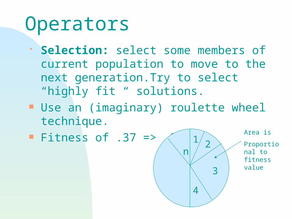
Operators Selection: select some members of current
population to move to the next generation.Try to select “highly fit “ solutions.
Use an (imaginary) roulette wheel technique. Fitness of .37 => 37%
21n
3
4
Area is
Proportional to fitness value
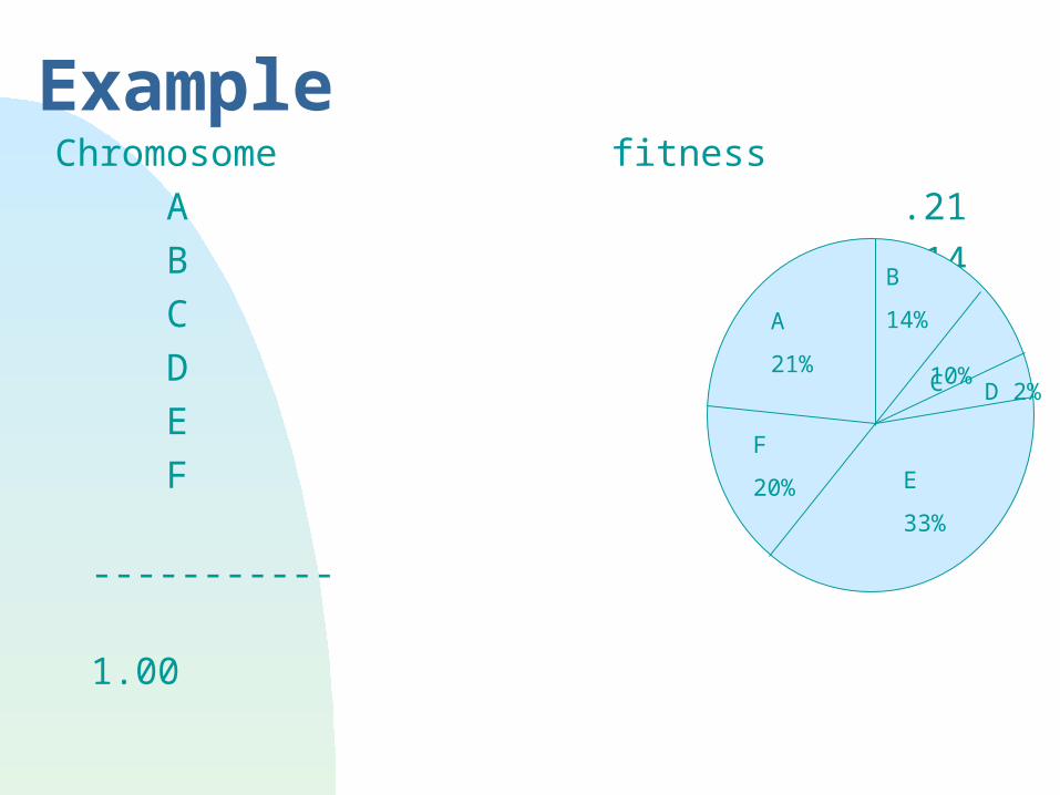
ExampleChromosome fitness
A .21
B .14
C .10
D .02
E .33
F .20
-----------
1.00
A
21% D 2%
10%
F
20% E
33%
B
14%
C
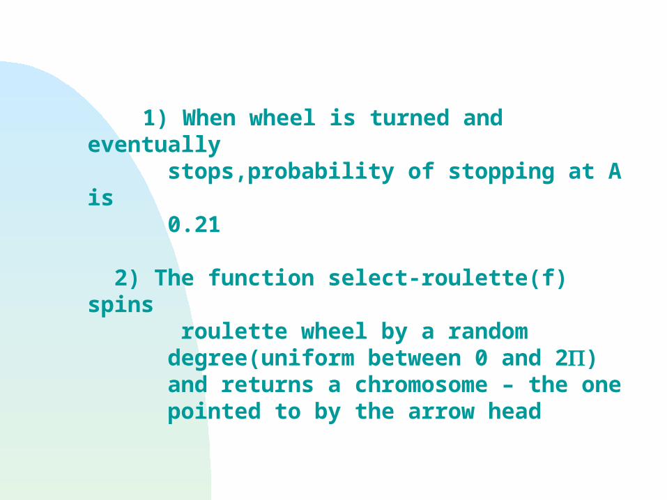
1) When wheel is turned and eventually stops,probability of stopping at A is 0.21
2) The function select-roulette(f) spins roulette wheel by a random degree(uniform between 0 and 2) and returns a chromosome – the one pointed to by the arrow head
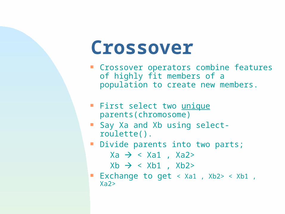
Crossover Crossover operators combine features of
highly fit members of a population to create new members.
First select two unique parents(chromosome)
Say Xa and Xb using select-roulette(). Divide parents into two parts; Xa < Xa1 , Xa2> Xb < Xb1 , Xb2> Exchange to get < Xa1 , Xb2> < Xb1 , Xa2>

This is a mating process of highly fit members.
Example: Often bit strings are used to
represent a chromosome.
Xa;100011;1110 ya;100011;1010
Xb;101010;1010 yb;101010;1110

Mutation Mutation operators randomly alters
structure of chromosome. Pm - user supplied
probability .Select a chromosome with probability,Pm usually;.05<Pm<0.2.
Mutation used to introduce new features into a population.
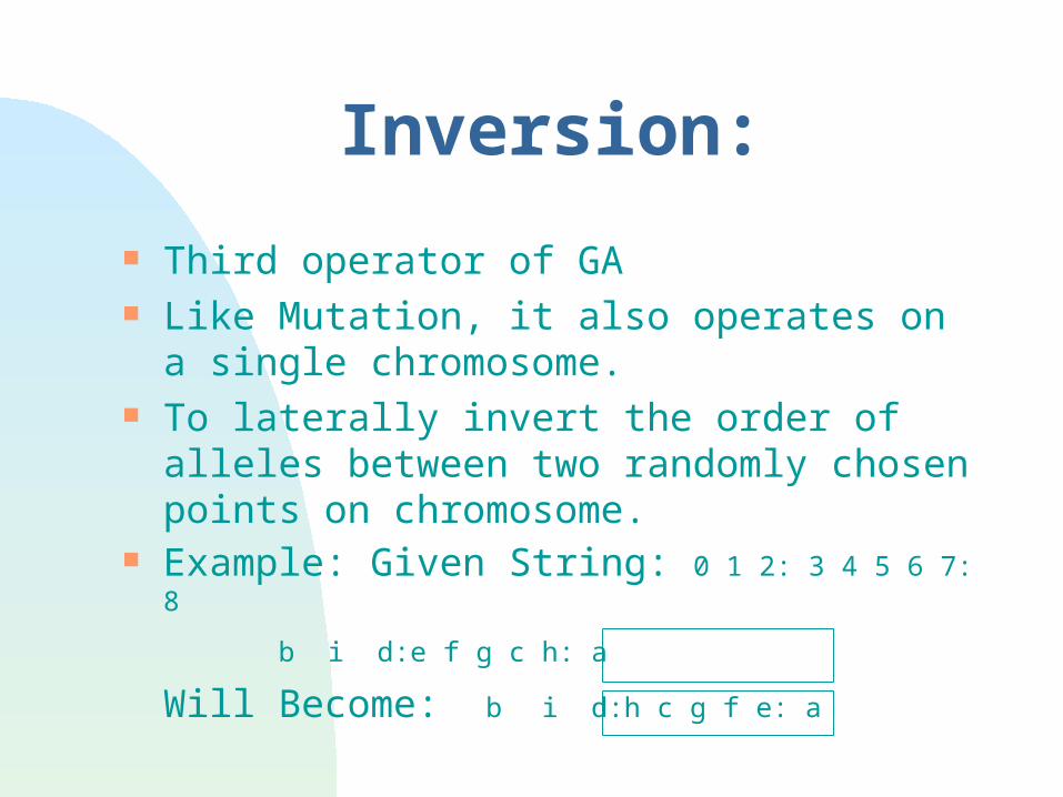
Inversion:
Third operator of GA Like Mutation, it also operates on a single
chromosome. To laterally invert the order of alleles
between two randomly chosen points on chromosome.
Example: Given String: 0 1 2: 3 4 5 6 7: 8
b i d:e f g c h: a
Will Become: b i d:h c g f e: a

Representation
Often a chromosome is encoded as a bit stream. The actual representation might be a structure,such as a floorplan, placement or route(wire).
By operating on bitstream one can generate a bit stream that doesn’t correspond to a legal structure.
Thus non bit string representations are often used including graphs and lists.
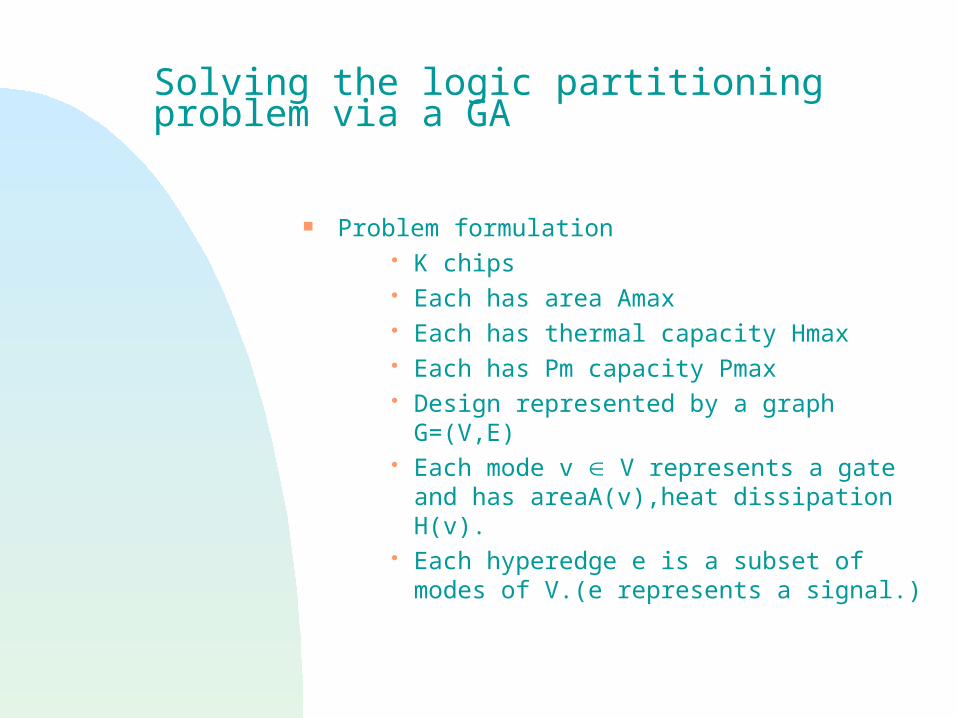
Solving the logic partitioning problem via a GA
Problem formulation K chips Each has area Amax Each has thermal capacity Hmax Each has Pm capacity Pmax Design represented by a graph G=(V,E) Each mode v V represents a gate and
has areaA(v),heat dissipation H(v). Each hyperedge e is a subset of modes of
V.(e represents a signal.)
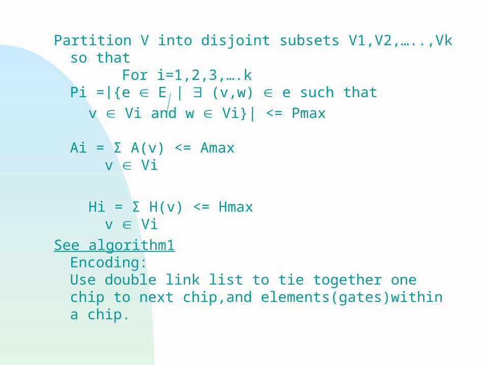
Partition V into disjoint subsets V1,V2,…..,Vk so that
For i=1,2,3,….kPi ={e E | (v,w) e such that
v Vi and w Vi}| <= Pmax Ai = Σ A(v) <= Amax v Vi
Hi = Σ H(v) <= Hmax v Vi
See algorithm1Encoding:Use double link list to tie together one chip to next chip,and elements(gates)within a chip.
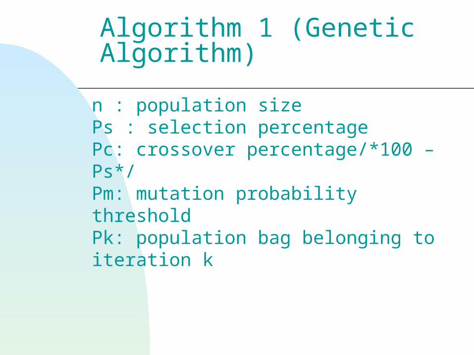
Algorithm 1 (Genetic Algorithm)
n : population sizePs : selection percentagePc: crossover percentage/*100 – Ps*/Pm: mutation probability thresholdPk: population bag belonging to iteration k
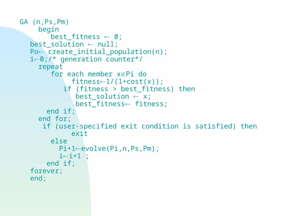
GA (n,Ps,Pm)
begin best_fitness 0;best_solution null;Po create_initial_population(n);i0;/* generation counter*/ repeat for each member xPi do fitness1/(1+cost(x)); if (fitness > best_fitness) then best_solution x; best_fitness fitness; end if; end for; if (user-specified exit condition is satisfied) then exit else Pi+1evolve(Pi,n,Ps,Pm); ii+1 ; end if;forever;end;
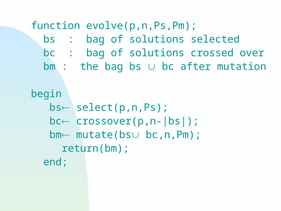
function evolve(p,n,Ps,Pm); bs : bag of solutions selected bc : bag of solutions crossed over bm : the bag bs bc after mutation begin bs select(p,n,Ps); bc crossover(p,n-|bs|); bm mutate(bs bc,n,Pm); return(bm); end;

function select(p,n,Ps) begin bs {}; i 0; while(i<Ps *n) do x select_roulette(p); bs bs {x}; ii+1; end while;return(bs) end;
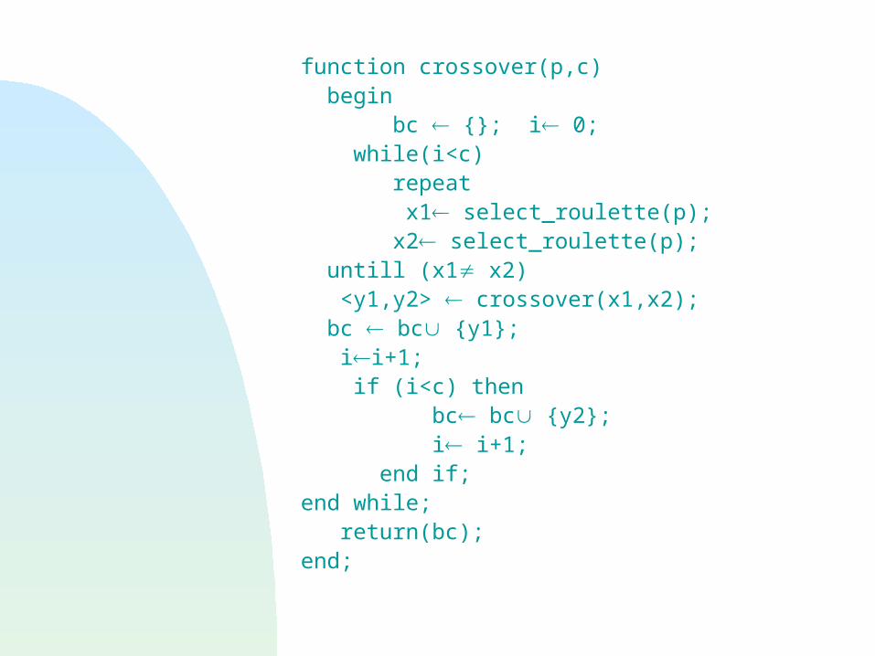
function crossover(p,c) begin bc {}; i 0; while(i<c) repeat x1 select_roulette(p); x2 select_roulette(p); untill (x1 x2) <y1,y2> crossover(x1,x2); bc bc {y1}; ii+1; if (i<c) then bc bc {y2}; i i+1; end if;end while; return(bc);end;
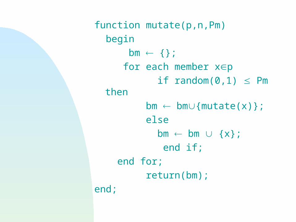
function mutate(p,n,Pm)
begin
bm {};
for each member xp
if random(0,1) Pm then
bm bm{mutate(x)};
else
bm bm {x};
end if;
end for;
return(bm);
end;

Figure 1: Representation scheme for a structure
Chip0
R15R14R6R5R1
R11R0
R12R7R2
R4R3
R10R8
chip1
R13R9chip4
chip3
chip2
Ri:components of a design(gates)
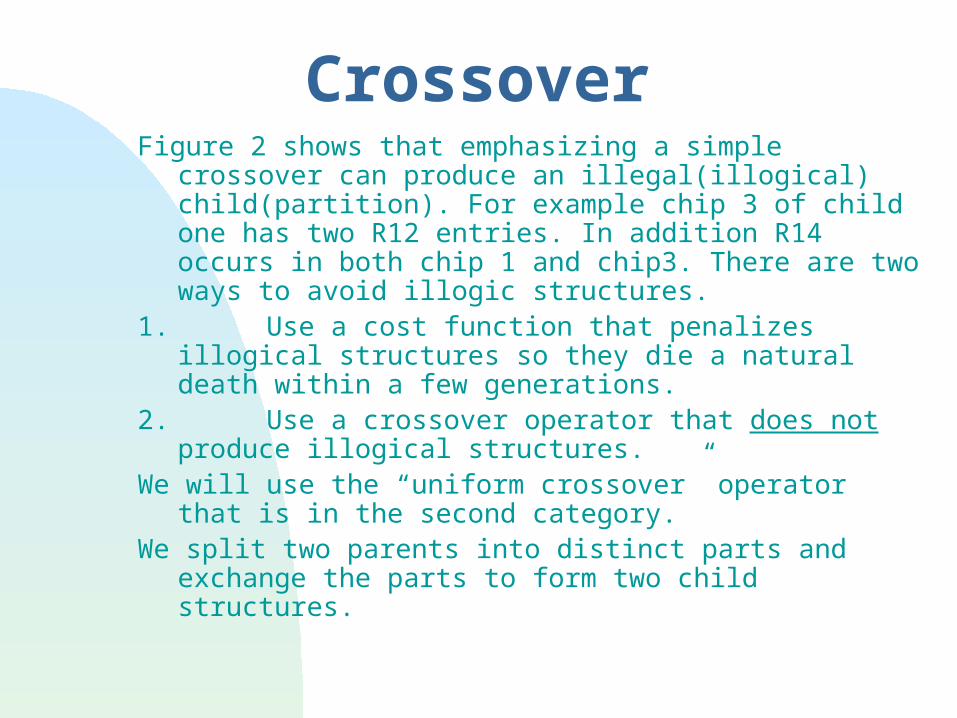
CrossoverFigure 2 shows that emphasizing a simple crossover
can produce an illegal(illogical) child(partition). For example chip 3 of child one has two R12 entries. In addition R14 occurs in both chip 1 and chip3. There are two ways to avoid illogic structures.
1. Use a cost function that penalizes illogical structures so they die a natural death within a few generations.
2. Use a crossover operator that does not produce illogical structures.
We will use the “uniform crossover” operator that is in the second category.
We split two parents into distinct parts and exchange the parts to form two child structures.
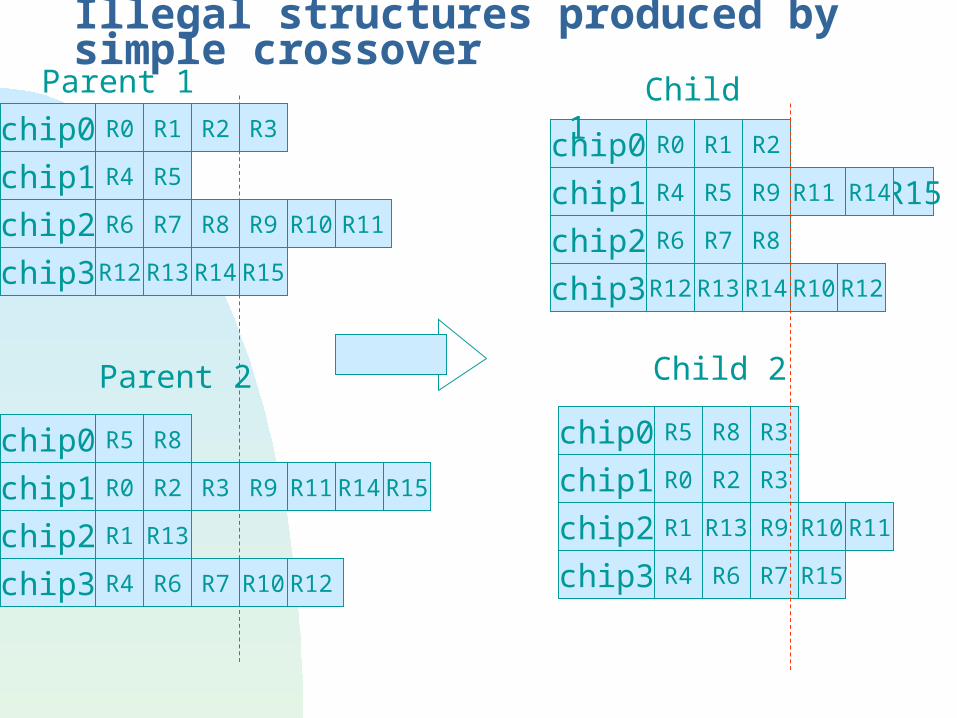
Illegal structures produced by simple crossover
chip0
chip1
chip3
chip2
chip1
chip0
chip2
chip1
chip0
chip3
chip2
chip0
chip3
chip3
chip2
chip1
R4R15
R6R4
R13R1
R15R14R11R9R3R2R0
R8R5
R11
R1
R3R2R0
R3R8R5
R12R10R7
R9R5R4
R2R1R0
R15R7R6R4
R11R10R9R13
R10R9R8R7R6
R15R14R13R12R12R10R14R13R12
R8R7R6
R14
R3
R5
R2R1
R11
R0
Parent 1 Child 1
Parent 2 Child 2
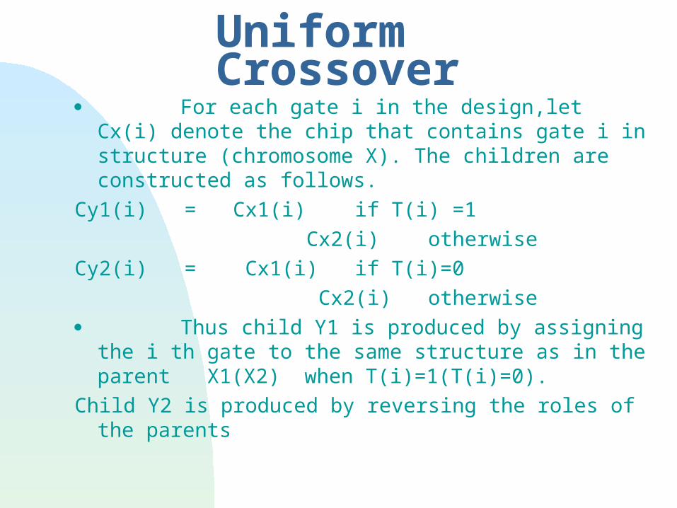
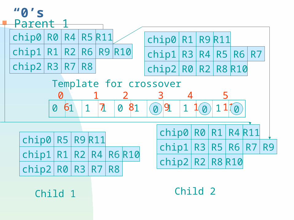
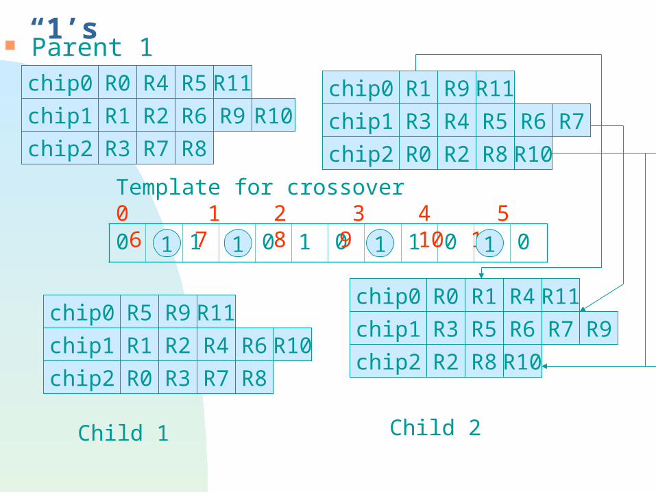
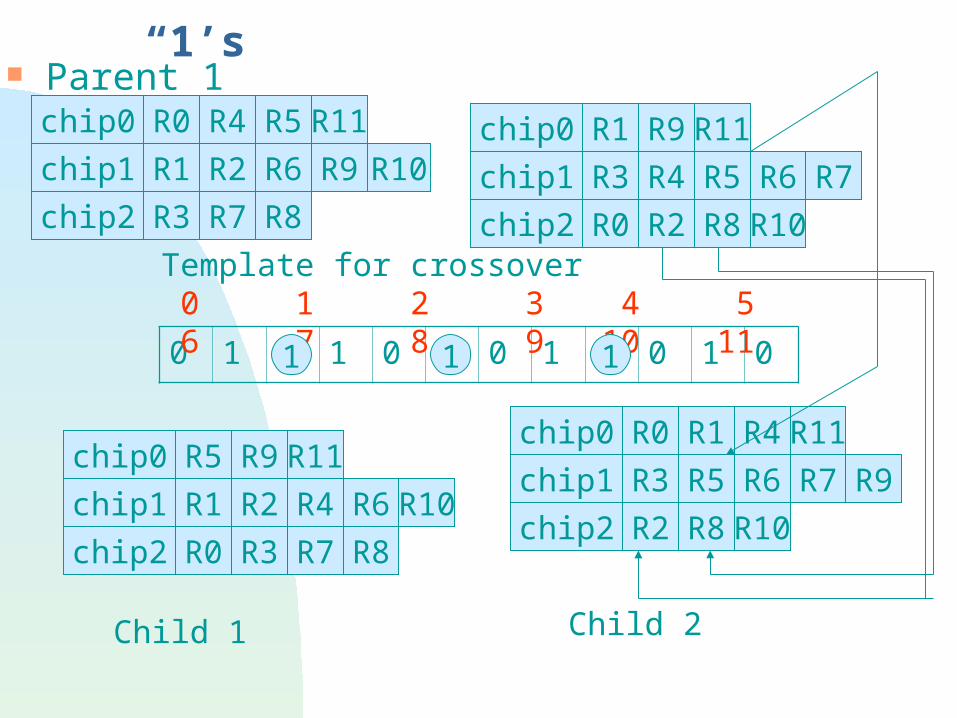
Uniform Crossover For each gate i in the design,let Cx(i) denote the
chip that contains gate i in structure (chromosome X). The children are constructed as follows.
Cy1(i) = Cx1(i) if T(i) =1
Cx2(i) otherwise
Cy2(i) = Cx1(i) if T(i)=0
Cx2(i) otherwise
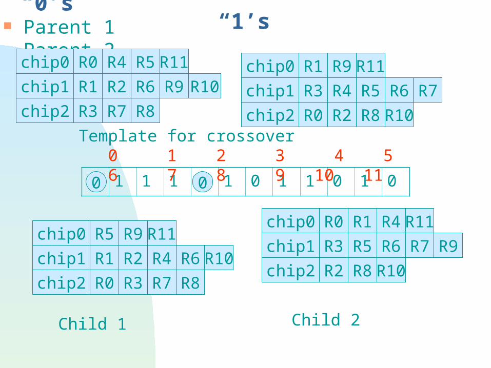
Thus child Y1 is produced by assigning the i th gate to the same structure as in the parent X1(X2) when T(i)=1(T(i)=0).
Child Y2 is produced by reversing the roles of the parents
Parent 1 Parent 2
chip0 R0 R4
R9
R11R5
R6
R10R8R2R0
R7R6R5R4R3
R11R9R1
R7R3R0
R10R6R4R2R1
R11R9R5R9R7R6R5R3
R11R4R1R0
R8
R2
R8R7R3
R1
R10R8R2
chip1
chip0
chip2
chip1
chip0
chip2
chip1
chip0
chip2
chip2
chip1
R10
Child 1 Child 2
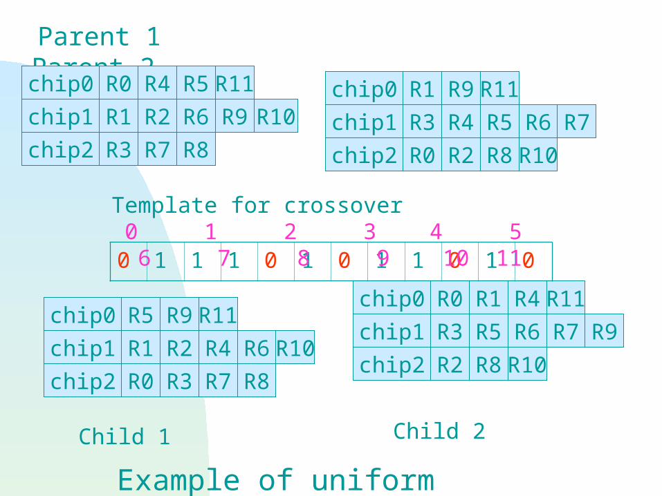
0 1 1 1 0 1 0 1 1 0 1 0
Template for crossover 0 1 2 3 4 5 6 7 8 9 10 11
Example of uniform crossover
“0’s” “1’s” Parent 1 Parent 2
chip0 R0 R4
R9
R11R5
R6
R10R8R2R0
R7R6R5R4R3
R11R9R1
R7R3R0
R10R6R4R2R1
R11R9R5R9R7R6R5R3
R11R4R1R0
R8
R2
R8R7R3
R1
R10R8R2
chip1
chip0
chip2
chip1
chip0
chip2
chip1
chip0
chip2
chip2
chip1
R10
Child 1 Child 2
0 1 1 1 0 1 0 1 1 0 1 0
Template for crossover 0 1 2 3 4 5 6 7 8 9 10 11
0 0
“0’s” Parent 1 parent 2
chip0 R0 R4
R9
R11R5
R6
R10R8R2R0
R7R6R5R4R3
R11R9R1
R7R3R0
R10R6R4R2R1
R11R9R5R9R7R6R5R3
R11R4R1R0
R8
R2
R8R7R3
R1
R10R8R2
chip1
chip0
chip2
chip1
chip0
chip2
chip1
chip0
chip2
chip2
chip1
R10
Child 1 Child 2
0 1 1 1 0 1 0 1 1 0 1 0
Template for crossover 0 1 2 3 4 5 6 7 8 9 10 11
00 0
“1’s” Parent 1 parent 2
chip0 R0 R4
R9
R11R5
R6
R10R8R2R0
R7R6R5R4R3
R11R9R1
R7R3R0
R10R6R4R2R1
R11R9R5R9R7R6R5R3
R11R4R1R0
R8
R2
R8R7R3
R1
R10R8R2
chip1
chip0
chip2
chip1
chip0
chip2
chip1
chip0
chip2
chip2
chip1
R10
Child 1 Child 2
0 1 1 1 0 1 0 1 1 0 1 0
Template for crossover0 1 2 3 4 5 6 7 8 9 10 11
1 111
“1’s” Parent 1 parent 2
chip0 R0 R4
R9
R11R5
R6
R10R8R2R0
R7R6R5R4R3
R11R9R1
R7R3R0
R10R6R4R2R1
R11R9R5R9R7R6R5R3
R11R4R1R0
R8
R2
R8R7R3
R1
R10R8R2
chip1
chip0
chip2
chip1
chip0
chip2
chip1
chip0
chip2
chip2
chip1
R10
Child 1 Child 2
0 1 1 1 0 1 0 1 1 0 1 0
Template for crossover 0 1 2 3 4 5 6 7 8 9 10 11
111
T-a binary string whose length is the number of elements to be partitioned.T is also called a template.
Randomly set the bits in T to 0 and 1.
Select two parent structures X1 and X2 for mating.
Let Y1 and Y2 children resulting from crossover.
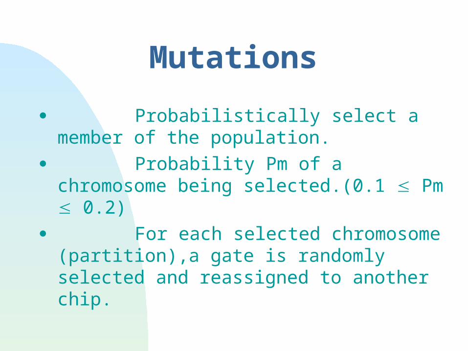
Mutations
Probabilistically select a member of the population.
Probability Pm of a chromosome being selected.(0.1 Pm 0.2)
For each selected chromosome (partition),a gate is randomly selected and reassigned to another chip.
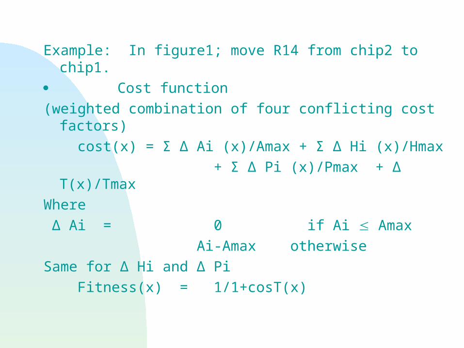
Example: In figure1; move R14 from chip2 to chip1.
Cost function
(weighted combination of four conflicting cost factors)
cost(x) = Σ Δ Ai (x)/Amax + Σ Δ Hi (x)/Hmax
+ Σ Δ Pi (x)/Pmax + Δ T(x)/Tmax
Where
Δ Ai = 0 if Ai Amax
Ai-Amax otherwise
Same for Δ Hi and Δ Pi
Fitness(x) = 1/1+cosT(x)
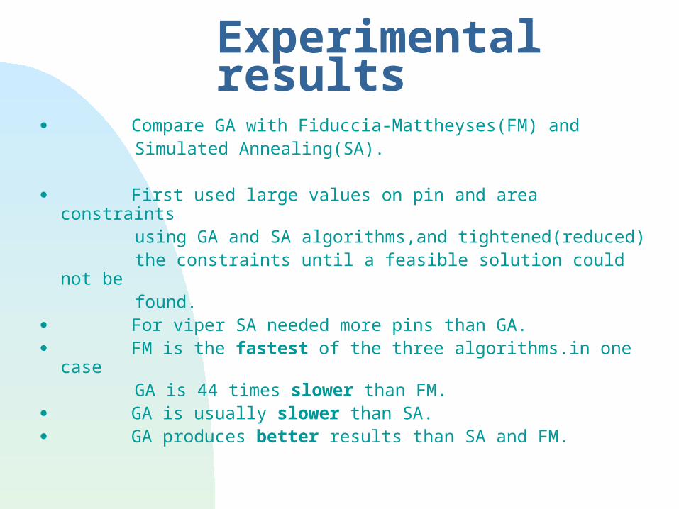
Experimental results
Compare GA with Fiduccia-Mattheyses(FM) and Simulated Annealing(SA). First used large values on pin and area constraints using GA and SA algorithms,and tightened(reduced) the constraints until a feasible solution could not be found. For viper SA needed more pins than GA. FM is the fastest of the three algorithms.in one case GA is 44 times slower than FM. GA is usually slower than SA. GA produces better results than SA and FM.
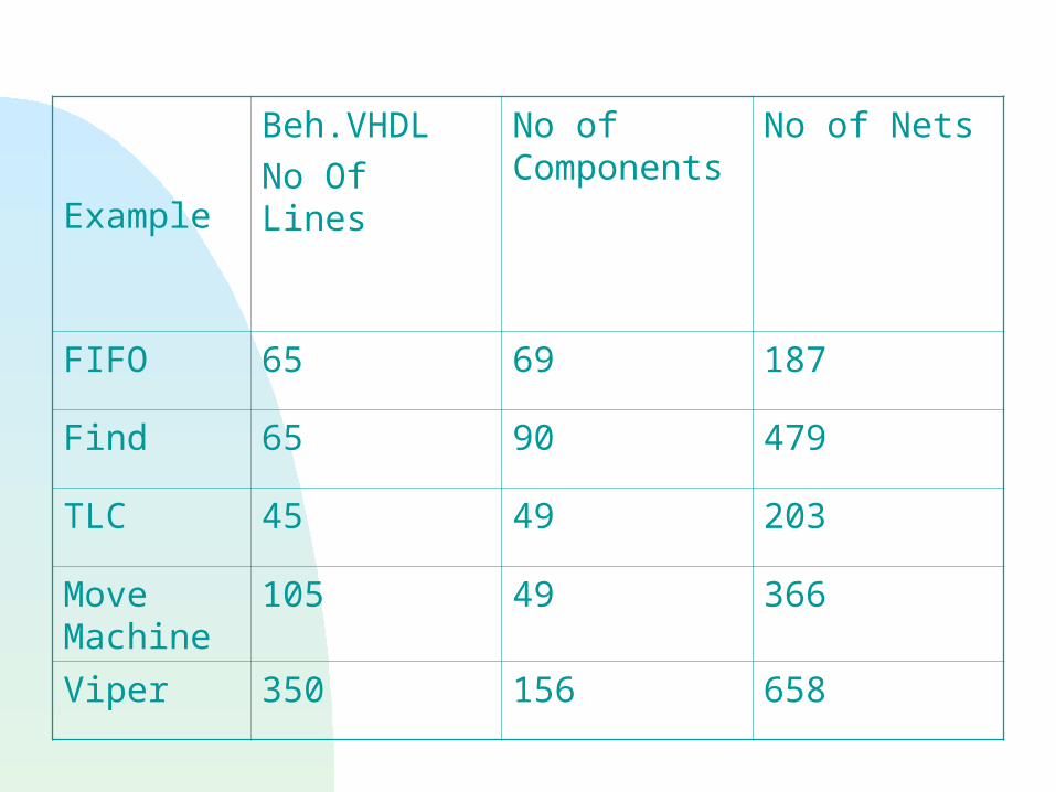
Example
Beh.VHDL
No Of Lines
No of Components
No of Nets
FIFO 65 69 187
Find 65 90 479
TLC 45 49 203
Move Machine
105 49 366
Viper 350 156 658
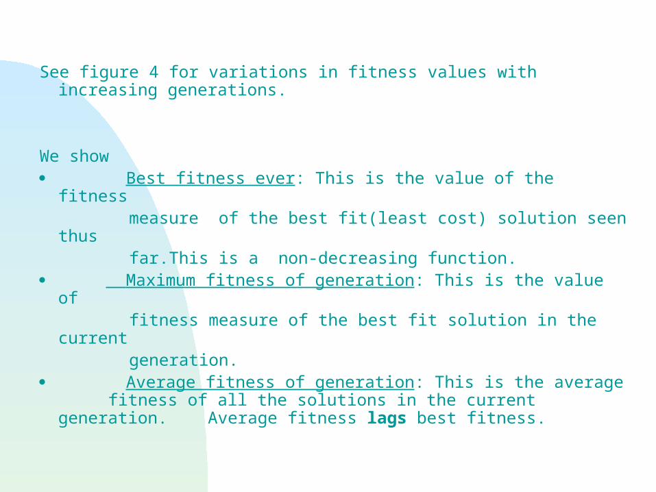
See figure 4 for variations in fitness values with increasing generations.
We show Best fitness ever: This is the value of the fitness measure of the best fit(least cost) solution seen thus far.This is a non-decreasing function. Maximum fitness of generation: This is the value of fitness measure of the best fit solution in the current generation. Average fitness of generation: This is the average
fitness of all the solutions in the current generation. Average fitness lags best fitness.
Placement via GA G=(V,E) – hypergraph. V- gates E- nets Assume a Gate Array layout structure. Assign(place) each gate to a unique slot(position). S= {S1,S2,….Src} set of slots. Slots are arranged into rows and columns;r-rows,c- columns. r.c > p - where |v| = p is number of gates. For a given placement,its associated length L is given by L = Σ L(e) where L(e) is an estimate of the length of eεE interconnect (wire) needed to route net e. Find an assignment so that L is minimal.
Genetic Encoding and operators
Encoding
Assume placement consists
of a rectangular grid of slots
as shown in the figure on the
next slide.
Encoding Dummy Gates
Row 4
Row 3
Row 2
Row 1
Row 0
C4 C3
C9
D6
C5C12D5
D7C10
C14C13C7C1D3
C8 C18 C2 D4 C6
C11
C15D2C17D1C16
Col 0 Col 1 Col 2 Col 3 Col 4
Chip
Empty Slot Occupied Slot
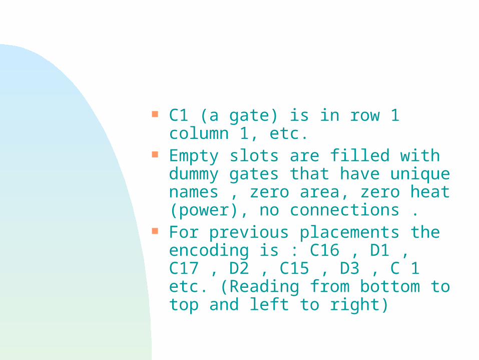
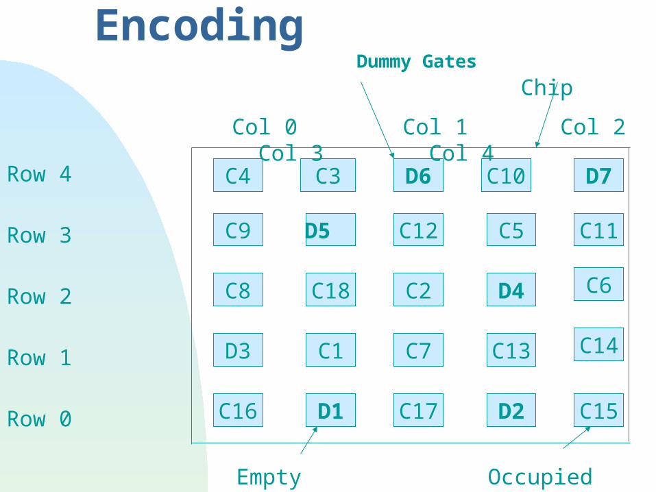
C1 (a gate) is in row 1 column 1, etc.
Empty slots are filled with dummy gates that have unique names , zero area, zero heat (power), no connections .
For previous placements the encoding is : C16 , D1 , C17 , D2 , C15 , D3 , C 1 etc. (Reading from bottom to top and left to right)

G
CBA
FED
IH End
Start
A B C D E F G H I
Encoding Using for Placement
Cross Over
A B E A BA B C D E
D C E A B D C C D E
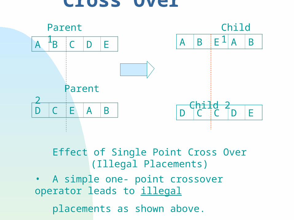
Effect of Single Point Cross Over (Illegal Placements)
• A simple one- point crossover operator leads to illegal
placements as shown above.
Parent 1 Child 1
Parent 2 Child 2

Child 1 has 2 A’s and 2 B’s , no C or D .
Child 2 has 2 D’s and 2 C’s no A or B
To resolve this, we employ a cycle crossover operator .
Cycle Crossover
Let P1 and P2 denote the 2 parents & C1 and C2 denote the 2 children .
Let P1 , P2 , C1 , C2 arrays be of size r.c

Child C1 is formed by first copying a number of genes (gate positions ) in P1 into C1 , and then filling the rest of the genes in C1 from P2 .
First , C1[0] P1[0] Let location i in P1contain the gate that
occupies position 0 in P2 Then C1[i]P1[i]. Continue this process . That if we just filled position i in C1 by copying position i in P1 , then we identify the gate in position i in P2 and determine the location j of that gate in P1 and copy that gate to position j in C1 .

This process halts when we get to a gate that has already been copied into C1. This completes a cycle .
Subsequently , we fill each unfilled position X in C1 by copying from P2 the gate assignments at X , i.e
C1[X]P2[X].
To form C2 carry out the same process while interchanging the role of P1 and P2

Example
P1 = I H B A G D E C F
P2 = A B C D E F G H I
I = 0 1 2 3 4 5 6 7 8
C1 = B C E G H
C2 = H B G E C A
D F
IFD
I A
Cycle Crossover
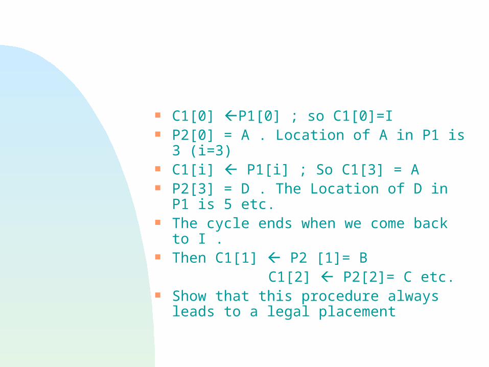
C1[0] P1[0] ; so C1[0]=I P2[0] = A . Location of A in P1 is 3 (i=3) C1[i] P1[i] ; So C1[3] = A P2[3] = D . The Location of D in P1 is 5
etc. The cycle ends when we come back to
I . Then C1[1] P2 [1]= B C1[2] P2[2]= C etc. Show that this procedure always leads to
a legal placement

GA in placement (Module Assignment):
b 4 c 7 e g
1 1 3 6 7
a d i f h
3 2 4 8
(a) Design given in a form of a graph
7 8 9 d e f
4 5 6 c b i
1 2 3 a g h (b) Partition Definition (c) One possible assignment

GA In-placement cont. Thus the string (below) represents the solution in
(c) 1 2 3 4 5 6 7 8 9 a g h c b i d e f with the fitness value of
1/85. Consider 2-modules g and f with the Manhattan
distance of 3 (2 vertically and 1 horizontally)The connection between g and f has a weight of 7,
thus for gf we have 7x3=21, doing as above for all assignments (in C) we get 85.
Other possible solutions: b d e f i g c h a with fitness 1/110 i h a g b f c e d with fitness 1/95
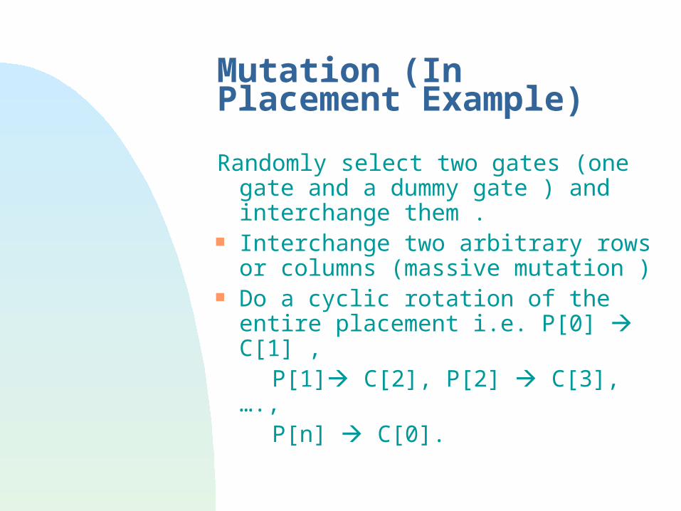
Mutation (In Placement Example)
Randomly select two gates (one gate and a dummy gate ) and interchange them .
Interchange two arbitrary rows or columns (massive mutation )
Do a cyclic rotation of the entire placement i.e. P[0] C[1] ,
P[1] C[2], P[2] C[3], …., P[n] C[0].
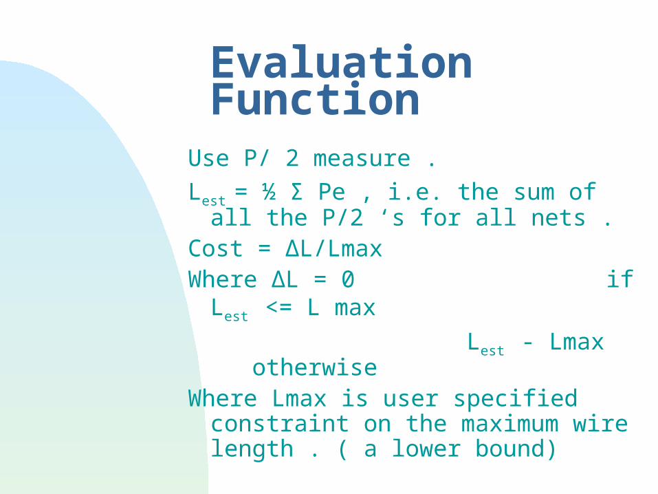
Evaluation Function
Use P/ 2 measure .
Lest = ½ Σ Pe , i.e. the sum of all the P/2 ‘s for all nets .
Cost = ΔL/Lmax
Where ΔL = 0 if Lest <= L max
Lest - Lmax otherwiseWhere Lmax is user specified
constraint on the maximum wire length . ( a lower bound)
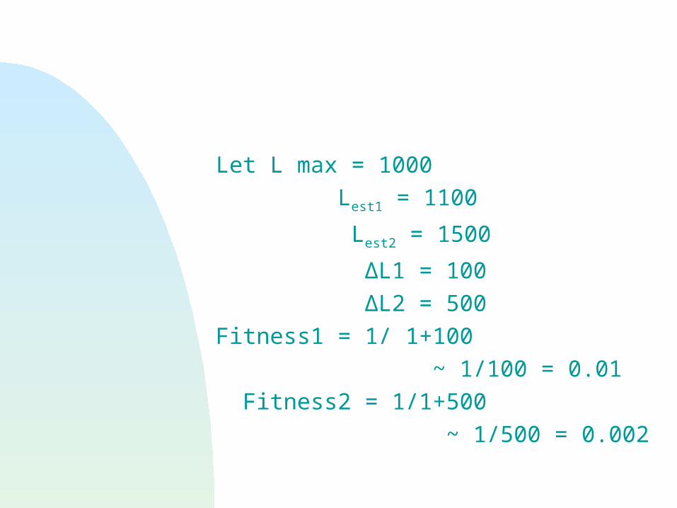
Let L max = 1000
Lest1 = 1100
Lest2 = 1500
ΔL1 = 100
ΔL2 = 500
Fitness1 = 1/ 1+100
~ 1/100 = 0.01
Fitness2 = 1/1+500
~ 1/500 = 0.002
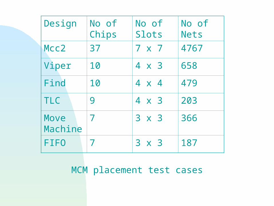
Design No of
Chips No of Slots
No of Nets
Mcc2 37 7 x 7 4767
Viper 10 4 x 3 658
Find 10 4 x 4 479
TLC 9 4 x 3 203
Move Machine
7 3 x 3 366
FIFO 7 3 x 3 187
MCM placement test cases
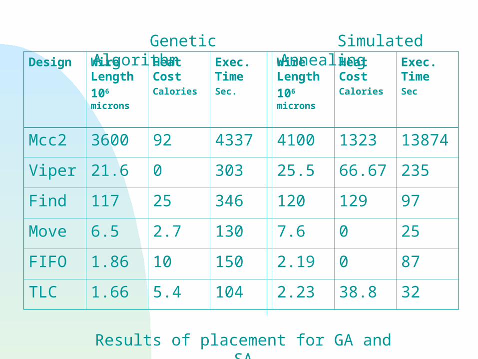
Design Wire
Length106 microns
Heat Cost Calories
Exec. Time Sec.
Wire Length106 microns
Heat Cost Calories
Exec. Time Sec
Mcc2 3600 92 4337 4100 1323 13874
Viper 21.6 0 303 25.5 66.67 235
Find 117 25 346 120 129 97
Move 6.5 2.7 130 7.6 0 25
FIFO 1.86 10 150 2.19 0 87
TLC 1.66 5.4 104 2.23 38.8 32
Genetic Algorithm Simulated Annealing
Results of placement for GA and SA
Results
GA produced better results than SA .
For one large problem it was even faster than SA
For large problems where convergence is slow GA is better because one can make use of the multiple solutions (chromosomes).

Review of partitioning
Why – what are the constraints and objectives? What entities get partitioned?
PCB,MCM,chips,etc.
Is partitioning done on functional or structural
information? Techniques: Initial construction serial or parallel.
Conjunctions and disjunctions Kernighan and Lin (K-L) Fiduccia-Mattheyses (F-M) Min-Cut (M-C) Simulated Annealing(SA) Genetic Algorithm(GA) Randomness in an effective technique Same constraints are non-monotonic Cut nets not edges See recent directions in netlist partitioning: A survey by”c.albert and B.kahng”,VLSI integration, pp.1- 81,1995
Categories of techniques
1. Move-based approaches2. Geometric representations3. Combinational formulations4. Clustering approaches
Techniques not discussed 1 Hall’s quadratic placement
2 Vector partitioning3 Dynamic programming4 Min delay5 Max-flow min-cut6 Bipartite flow7 Mathematical programming
Functional partitioning