randomized algorithms and probabilistic analysis of · pdf filerandomized algorithms and...

Lecture: Randomized AlgorithmsTU/e 5MD20

↩

5MD20—Design AutomationRandomized Algorithms and Probabilistic Analysis of Algorithms

1

Phillip Stanley-Marbell

keynote:/Users/pip/MY-TALKS/HiPEAC07/hipeac07.key?id=BGSlide-93



↩

Lecture Outline

• Motivation

• Probability Theory Refresher

• Example Randomized Algorithm and Analysis

• Tail Distribution Bounds

• Example Application of Tail Bounds

• Chernoff Bounds

• The Probabilistic Method

• Hashing

• Summary of Key Ideas

2




↩

What are Randomized Algorithms and Analyses?

• Randomized algorithms– Algorithms that make random decisions during their execution

– Example: Quicksort with a random pivot

• Probabilistic analysis of algorithms– Using probability theory to analyze the behavior of (randomized or deterministic) algorithms

– Example: determining the probability of a collision of a hash function

3

Probability and Computation

Randomized Algorithms Probabilistic Analysis of algorithms

Monte Carlo algorithms

Las Vegas algorithms

May fail or return an incorrect answer

Always return right answer




↩

Why Randomized Algorithms and Analyses?

• Why randomized algorithms?– Many NP-hard problems may be easy to solve for “typical” inputs

– One approach is to use heuristics to deal with pathological inputs

– Another approach is to use randomization (of inputs, or of algorithm) to reduce the chance of worst-case behavior

4








↩

Why Randomized Algorithms and Analyses?

• Why probabilistic analysis of algorithms?– Naturally, if algorithm makes random decisions, performance is not deterministic

– Also, deterministic algorithm behavior may vary with inputs

– Probabilistic analysis also lets us estimate bounds on behavior; we’ll talk about such bounds today

5








↩

Theoretical Foundations

• Probability theory (things you covered in 2S610, 2nd year)– Probability spaces

– Events

– Random variables

– Characteristics of random variables

• Combinatorics & number theory (some things you might have seen in 2DE*)– Many relations come in handy in simplifying analysis

• Algorithm analysis

• We will review relevant material in the next half hour

6




↩

Lecture Outline

• Motivation





• Chernoff Bounds


• Hashing


7




↩

Probability Theory Refresher

• Probability space, (Ω, ℱ,℘), defines– The possible occurrences (simple events), sets of occurrences (subsets of Ω), and “likelihood” of occurrences

• Sample space, Ω– Composed of all the basic events we are concerned with

– Example: for a coin toss, Ω = {H, T}

• Sigma algebra, ℱ– Possible occurrences we can build out of Ω– Example: for coin toss, ℱ = {∅, Ω, H, T}

– Events are members of ℱ

• Probability measure, ℘– A mapping from ℱ to [0, 1]

– Assigns probability (a real number p ∈ [0, 1]) to events

– One example of a probability measure is a probability mass function

8




↩

Notation

• Event sets– Will start today by representing events with sets, using letters early in the alphabet e.g., A, B, ...

– Events may be unitary elements or subsets of Ω

• Probability– Probability of event A will be written as Pr{A}

9

e1

e2

e3

e4

e5

e6

e7

e8

Ω




↩

Independence, Disjoint Events, and Unions

• Two events, A and B are said to be independent, iff – Occurrence of A does not influence outcome of B

– Pr{A∩B} = Pr{A}·Pr{B}

• Note that this is different form events being mutually exclusive– If two events A and B are mutually exclusive, then Pr{A∩B} = ∅

• For any two events E1 and E2

– Pr{E1∪E2} = Pr{E1} + Pr{E2} − Pr{E1 ∩ E2}

• Union bound (often comes in handy in probabilistic analysis)

10

Pr !i ! 1"Ei "

i ! 1Pr"#Ei$≤




↩

Conditional Probability

• Probability of event B occurring, given A has occurred, Pr{B | A}– Pr{B | A} = Pr{B ∩ A}

– Pr{A}

• If events A and B are independent:– Pr{B ∩ A} = Pr{B}·Pr{A}

– Pr{B | A} = Pr{B ∩ A}

– Pr{A}

– Pr{B | A} = Pr{B}·Pr{A} = Pr{B}

– Pr{A}

11




↩

Events and Random Variables

• So far, we have talked about probability and independence of events– Rather than work with sets, we can map events to real values

• Random Variables– A random variable is a function on the elements of the sample space, Ω, used to identify elements of ℱ.

– Definition: A random variable, X on a sample space Ω is a real-valued function on Ω; i.e., X : Ω→ℝ.– We will only deal with discrete random variables, which take on a finite or countably infinite number of values

• Random variables define events– The occurrence of a random variable taking on a specific value defines an event

– Example: Coin toss. Let X be a random variable defining the number of heads resulting from a coin toss– Sample space, Ω = {H, T}, sigma algebra of subsets of Ω, ℱ = {∅, Ω, {H}, {T}}

– X: {∅, Ω, {H}, {T}} → {0, 1}

– Events: {X = 0}, {X = 1}

– In general, an event defined on a random variable X is of the form {s ∈ Ω | X(s) = x }

12




↩

Notation

• Will represent random variables with uppercase letters, late in alphabet– Example: X, Y, Z

– Will use the abbreviation rvar for “random variable”

• Events– Events correspond to a random variable, say, X, (uppercase) taking on a specific value, say, x (lowercase)

– Probability of rvar X taking on the specific value x is written as Pr{X = x} or fX (x)

– Example: Coin toss — Let X be an rvar representing number of heads; Pr{X = 0} = fX(0) = ½ (for a fair coin)

–

13




↩

Random Variables — Intuition

• So far, we’ve presented a lot of notation; can we gain more intuition ?

• Imagine a phenomenon, that can be represented w/ real values– Example: the result of rolling a die

– Let X and Y be functions mapping the result of rolling die to a number

– e.g., X = die result, : Ω→{1, 2, 3, 4, 5, 6} or Y = 2·(die result)+1 : Ω→{3, 5, 7, 9, 11, 13}

– X and Y are two different functions (random variables) defined on the same set of events

• Each time X takes on a specific value is an event– For the above die rolling example, with rvars X and Y:

– Pr{X = 1} = Pr{Y = 3}, Pr{X = 4} = Pr{Y = 9}, and so on

14




↩

Characteristics of Random Variables

• Random variables and events1. We first talked about random phenomenon events in terms of sets

2. We then introduced rvars, to let us represent events with real numbers

3. When representing events with rvars, we can then look at some measures or characteristics of event phenomena

• Link to randomized algorithms and analyses; will reason about:– Randomized algorithms in terms of rvars characterizing actions of the algorithm

– Probabilistic analysis of algorithms in terms of rvars characterizing properties of the alg. behavior given inputs

15








↩

Characteristics of Random Variables

• Expectation or Expected Value, E[X], of an rvar X

• Properties of E[X]– Linearity

– Constant multiplier

• Question– What is E[X·E[X ]] ?

16

E!X " !#x

x"fx"$x% E!X " !#i

i Pr"$X ! i%or

E!"i!1

n

"Xi# = "i!1

n

"E$Xi%E!c X " = cE!X "




↩

Common Discrete Distributions

• Uniform discrete– All values in range equally likely

– Ω = {a, ..., b}, ℱ = 2Ω, ℘: Pr{X=x} = 1/|Ω|

• Bernoulli or indicator random variable– Success or failure in a single trial

– Ω = {0, 1}, ℱ = 2{0, 1} = {∅, {0}, {1}, Ω}, ℘: Pr{X=0} = p, Pr{X=1} = 1-p– E[X] = p, Var[X] = p(1-p)

• Binomial– Number of successes in n trials

– Ω = ℤn+1 = {0, 1, 2, ..., n}, ℱ = 2Ω, ℘: fX(k) = pk(1-p)n-k – E[X] = np, Var[X] = np(1-p)

• Geometric– Number of trials before first failure

– Ω = ℕ ℱ = 2ℕ, ℘: fX (k) = p(1-p)k-1 – E[X] = 1/p, Var[X] = (1-p)/p2

17

( )nk




↩

Useful Mathematical Results

• Some useful results from number theory and combinatorics we’ll use later

18

!i!0

"

ri = 11#r!i!1

"

ri = r1#r!i!0

m

ri = 1"rm#1

1"r

1 - kn≈ e

- kn , when k is small compared to n

For any y, 1+y ≤ ey

!i!1

n1i = ln(n) + O(1)




↩

Lecture Outline

• Motivation





• Chernoff Bounds


• Hashing


19




↩

Quicksort

Input: A list S = {x1, ..., xn} of n distinct elements over a totally ordered universeOutput: The elements of S in sorted order

1. If S has one or zero elements, return S. Otherwise continue.2. Choose an element of S as a pivot; call it x3. Compare every other element of S to x in order to divide the other elements into two sublists

a. S1 has all the elements of S that are less than x;b. S2 has all those that are greater than x.

4. Apply Quicksort to S1 and S2

5. Return the list S1, x, S2

Probabilistic Analysis of Quicksort

• Worst case performance is Ω(n2)– E.g., if input list in decreasing order and pivot choice rule is ‘pick first element’

– On the other hand, if pivot always splits S into lists of approximately equal size, performance is O(n log n)

• Question:– Assuming we use the ‘pick first element’ pivot choice, and input elements are chosen from a uniform discrete

distribution on a range of values, what is the expected number of comparisons?

– i.e., let X be an rvar denoting number of comparisons; what is E[X] ?

20




↩


21

Theorem.

If the first list element is always chosen as pivot, and input is chosen uniformly at random from all possible permutations of values in input support set, then the expected number of comparisons made by Quicksort is 2n ln n + O(n)

Proof.

Given an input set x1, x2, ..., xn chosen uniformly at random from possible permutations, let y1, y2, ..., yn be the same values sorted in increasing order

Let Xij be an indicator rvar that takes on value 1 if yi and yj are compared at any point in the algorithm, 0 otherwise, for some i < j. The total number of comparisons, is the total number of times Xij = 1

Let X be an rvar denoting the total number of comparisons of Quicksort. Then,

X = !i!1n"1!j!i#1

n Xij and

where we’ve used the linearity property introduced on slide 16

E[X] = E!"i!1

n"1#"j!i$1

n Xij# = "i!1

n"1"j!i$1n E$Xij%




↩


22

Theorem.


Proof. (contd)

Since Xij is an indicator rvar, E[Xij] is the probability that Xij = 1 (from slide 17). But recall that Xij is the event that two elements yi and yj are compared.

Two elements yi and yj are compared iff either of them is first pivot selected by Quicksort from the set Yij = {yi, yi+1, ..., yj}. This is because if any other item in Yij were chosen as a pivot, since that item would lie between yi and yj, it would place yi and yj on different sublists (and they would never be compared to each other).

Now, the order in the sublists is the same as in original list (we are in process of sorting). From theorem, we always choose first element as pivot; since input is chosen uniformly at random from all possible permutations, any element of the ordering Yij is equally likely to be first in the (random ordered) input sublist.

Thus probability that yi or yj is selected as pivot, which is the probability that yi and yj are compared, which is the probability that Xij = 1, which is E[Xij], is (from definition of discrete uniform distribution on slide 17), 2/(j-i+1).




↩


23

Theorem.


Proof. (contd)

Substituting E[Xij] = 2/(j-i+1) into the expression for E[X] form slide 21:

E[X] = !i!1n"1!j!i#1

n 2j"i#1

= !i!1n"1!k!2

n"i#1 2k

= !k!2n !i!1

n"1"k 2k

= !k!2n "n" 1# k#$ 2

k

= $"n" 1#$!k!2n 2

k% # 2$"n# 1#

= "2$n" 2#$!k!1n 1

k# 4$n

= 2$n ln n " O"n# from slide 18




↩

Randomized Quicksort

• What if inputs are not the uniformly random selections of permutations?

• How to avoid pathological inputs? pick a random pivot!

• Analysis of number of comparisons is similar to foregoing analysis

24

Theorem.

Suppose that, whenever a pivot is chosen for Randomized Quicksort, it is chosen independently and uniformly distributed over all possibly choices. Then, for any input, the expected number of comparisons made by Randomized Quicksort is 2n ln n + O(n).

Proof.

Almost identical to proof of expected number of comparisons for deterministic Quicksort with randomized inputs.

Try doing this proof yourself as an exercise.




↩

Lecture Outline

• Motivation





• Chernoff Bounds


• Hashing


25




↩

Tail Distribution Bounds

• We’ve seen one example of measures for characterizing a distribution– Expectation, E[X] gives us an idea of the average value taken on by an rvar

• Another important characteristic is the tail distribution– Tail distribution is the probability that an rvar takes on values far from its expectation

– Useful in estimating the probability of failure of randomized algorithms

– Intuitively, one may think of it as Pr{|X-k| ≥ a}

• We will now look at a few different bounds on tail distribution– “Loose” bounds don’t tell us much; they are often however easier to calculate

– “Tight(er)” bounds give us a narrower range on values, but often require more information

26

Pr{

X =

x}

x

Pr{X ≥ a}

a




↩

Markov’s Inequality

• A loose bound that is easy to calculate is Markov’s inequality– We can easily calculate Pr{X ≥ a} knowing only the expectation of X

– This however often doesn’t tell us much!

• We will use a similar argument in the Probabilistic Method later today

27

Theorem [Markov’s Inequality].

Let X be a random variable that assumes only nonnegative values. Then, for all a > 0, Pr{X ≥ a} ≤ (E[X] /a)

Proof.

For a > 0, let I be a Bernoulli/indicator random variable, with I = 1 if X ≥ a, 0 otherwise. Since X is nonnegative, I ≤ X/a. From slide 17, E[I] = Pr{I = 1} = Pr{X ≥ a}, thusPr{X ≥ a} ≤ E[X/a] = E[X]/a (from slide 16).




↩

• To derive at tighter bounds, we will need the idea of moments of an rvar

• Definition: kth moment– The kth moment of an rvar X is E[Xk] ,

– k = 0 is termed the “first moment”, and so on

• Definition: variance– The variance of an rvar X is defined as Var[X] = E[(X− E[X])2]

– Exercise: Show that Var[X] = E[X2] - (E[X])2

• Definition: standard deviation– The standard deviation of an rvar X, is σ[X] = √Var[X ]

Moments

28




↩

Chebyshev’s Inequality

• Now that we know about Var[X], we can introduce a tighter bound on tail

29

Theorem [Chebyshev’s Inequality].

For any a > 0, Pr{|X − E[X ]| ≥ a} ≤ (Var[X ] /a2)

Proof.

Pr{|X − E[X ]| ≥ a} = Pr{(X − E[X ])2 ≥ a2}. Since (X − E[X ])2 is a nonnegative rvar, we can apply Markov’s inequality to yield:

Pr{(X − E[X ])2 ≥ a2} ≤ E[(X − E[X ])2]/a2 = (Var[X ] /a2).




↩

Lecture Outline

• Motivation





• Chernoff Bounds


• Hashing


30




↩

Randomized Algorithm for Median, RM

• Idea– Find two nearby elements d and u, spanning a small set C, by sampling S

– Since |C| is o(n/log n), can sorted it in o(n) time using alg. that is O(k log k) for k elements

– The check in step 7 is to validate that the set C is indeed small so that above assumption holds

31

Randomized Median Algorithm

Input: A set S of n elements over a totally ordered universeOutput: The median element of S, denoted m.

1. Pick a (multi-)set R of ⎡n3/4⎤elements in S, chosen independently and uniformly at random, with replacement.

2. Sort the set R.3. Let d be the (½n3/4 -√n)th smallest element in the sorted set R.4. Let u be the (½n3/4 +√n)th smallest element in the sorted set R.5. By comparing every element in S to d and u, compute the set C = {x ∈ S : d ≤ x ≤ u}

and the numbers ld = |{x ∈ S : x < d}| and lu = |{x ∈ S : x > u}| 6. If ld > n/2 or lu > n/2 then FAIL7. If |C | ≤ 4n3/4 then sort the set C, otherwise FAIL8. Output the (n/2- ld + 1)th element in the sorted order of C




↩

What is the probability that RM Fails?

• What can go wrong?– Sample might not be representative in terms of median:

– e1: Y1 = |{r ∈ R | r ≤ m}| < ½n3/4 − √n — too few elements in sample smaller than m,

– e1: Y1 = |{r ∈ R | r ≥ m}| < ½n3/4 − √n — too few elements in sample larger than m

– e3: |C | > 4n3/4 — sample picked from S has d and u too far apart

– Pr{RM fails} = Pr{e1 ∪ e2 ∪ e3} = Pr{e1} + Pr{e2} + Pr{e3}, since the events e are disjoint

• Let’s look at determining probability of event e1

32




↩

Reminder — Bernoulli/Indicator and Binomial

• Bernoulli or indicator rvar– Success or failure in a single trial

– Example: Coin toss, with rvar X = 1 when heads, X = 0 when tails

– Ω = {0, 1}

– Pr{X=0} = p, Pr{X=1} = 1-p

– E[X] = p

– Var[X] = p(1-p)

• Binomial rvar– Number of successes in n Bernoulli trials of parameter p

– Sum of n Bernoulli(p) rvars is a Binomial(n, p) rvar

– Ω = ℤn+1 = {0, 1, 2, ..., n},

– fX(k) = pk(1-p)n-k

– E[X] = np

– Var[X] = np(1-p)

33

( )nk




↩

Determining Pr{e1}

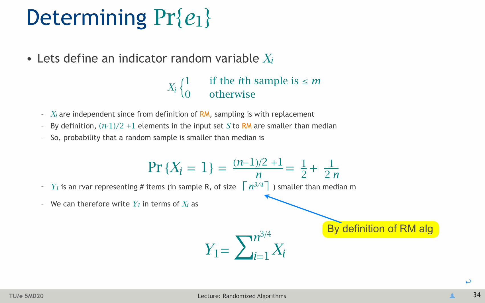
• Lets define an indicator random variable Xi

– Xi are independent since from definition of RM, sampling is with replacement

– By definition, (n-1)/2 +1 elements in the input set S to RM are smaller than median

– So, probability that a random sample is smaller than median is

– Y1 is an rvar representing # items (in sample R, of size ⎡n3/4⎤) smaller than median m

– We can therefore write Y1 in terms of Xi as

34

Xi !1 if the ith sample is ! m0 otherwise

Pr!!Xi " 1" " #n#1$%2 $1n

" 12$ 1

2!n

Y1!!i!1

n3"4Xi

By definition of RM alg




↩

Determining distribution of Y1

• Recall (slide 33) that sum of n Bernoulli(p) rvars is Binomial(n, p), so

• and

35

Y1!!i!1

n3"4Xi

fY1!y" ! n3#4

y"$ 1

2# 1

2"n %y "$ 12$ 12"n %n3#4$y

Var!Y1" ! n3#4$ 12" 1

2#n %#$ 12$ 12#n % E!Y1" ! n3#4$ 1

2" 1

2#n %




↩

Determining Pr{e1}

• Back to determining Pr{e1} (recall: it’s one of events in which RM fails)...– Pr{e1} = Pr{Y1 < ½n3/4 −√n}

– Even though we can determine distribution of rvar Y1, determining Pr{Y1 < y} is not easy

– (If we instead wanted Pr{Y1 ≤ y} that is just the cumulative distribution function of Y1)

– We could determine the appropriate limit of the above sum to give us Pr{Y1 < y}...

• We can however easily get a bound on Pr{e1}– We can apply Chebyshev’s inequality to get a bound on Pr{e1}:

36

Pr!!e1" " Pr!#Y1 # 12!n

34$ n $

% Pr!#%Y1 $ E&Y1'% & n $% Var&Y1'

n

" n$1

4 ( 12' 1

2!n )!( 12$ 12!n )




↩

Lecture Outline

• Motivation





• Chernoff Bounds


• Hashing


37




↩

• Bounds are useful!– We saw in previous example how knowing about the Chebyshev inequality helped us to quickly

answer questions about probability of failure of a randomized algorithm

• But, how tight are the bounds?– Not all bounds tell us something useful– Example: Pr{X = x} ≤ 1 is always true for any rvar X and value x, but it tells you nothing new

• Chernoff bounds give us tighter bounds on Pr{|X-E[X]| > a}

Chernoff Bounds

38

Pr{

X =

x}

xa

Loose bound

1.0

Tighter bound

Pr{X = a} (if X is a discrete rvar)




↩

Chernoff Bounds

• Unlike Markov and Chebyshev inequalities, these are a class of bounds– There are Chernoff bounds for different specific distributions

– Chernoff bounds are however all formulated in terms of moment generating functions

• Moment generating function for an rvar X, MX (t ) = E[etX]– MX (t ) uniquely characterizes distribution

– We will be most interested in the property that E[Xn] = MX (n)(0)

– i.e. nth derivative of MX (t ) at t = 0 yields E[Xn]

– Example: Moment generating function for Bernoulli rvar

– (Recall: coin toss, “heads” or “1” with probability p, “tails” or “0” (1-p)):

39

MX !t" ! E#etX $! pet 1"%1#p&$'et 0(! pet"%1#p&




↩

Pr!!X " a" # Pr!#etX" eta$$

E%etX &eta

$ mint%0!E%etX &

eta

Chernoff Bounds

• Chernoff bounds generally make use of the ff. (from Markov’s ineq., slide 7)

• For a sequence of independent (but not necessarily i.i.d.) indicator rvars– The following Chernoff bounds (which can be derived from the above) exist:

– For 0 < δ ≤ 1,

– For 0 < δ < 1,

40

for t>0

Pr!!X " a" # Pr!#etX$ eta$"

E%etX &eta

" mint%0!E%etX &

eta

for t<0

Pr!!X " "1#$#% $ & e'%$2

3

where u = E[X ]

Pr!!X " "1#$#% $ " e#%$2

2




↩

Chernoff Bounds — Estimating a Parameter

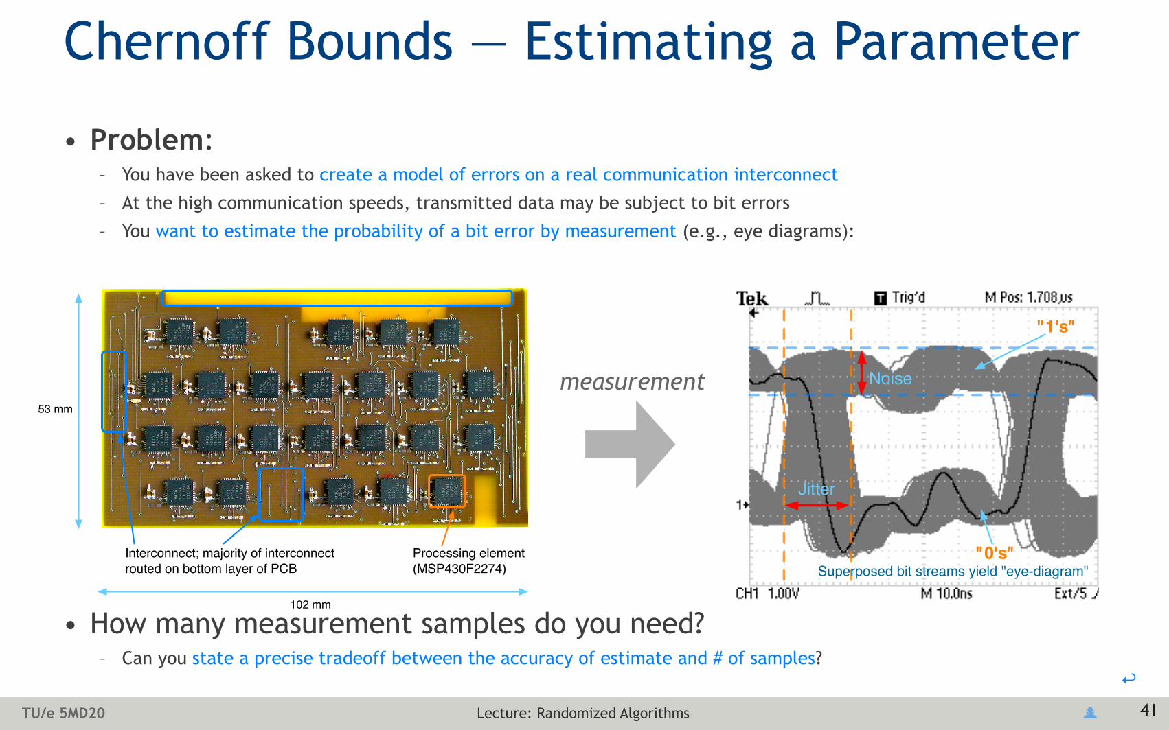
• Problem:– You have been asked to create a model of errors on a real communication interconnect

– At the high communication speeds, transmitted data may be subject to bit errors

– You want to estimate the probability of a bit error by measurement (e.g., eye diagrams):

• How many measurement samples do you need?– Can you state a precise tradeoff between the accuracy of estimate and # of samples?

41

Jitter

Noise

Superposed bit streams yield "eye-diagram"

"1's"

"0's"Processing element(MSP430F2274)

Ground and power-plane keep-out areas to reduce RF signal loss in test sensor node attached to module

Interconnect; majority of interconnect routed on bottom layer of PCB

53 mm

102 mm

measurement




↩


• Estimating probability of bit error from n measurements– Let p be the probability we are trying to estimate, taking n measurements– Let X = pn be the number of measurements in which we observe bit errors– If n is sufficiently large, we expect p to be close to p

• Confidence interval– A 1 - γ confidence interval for a parameter p is an interval [p-δ, p+δ] such that

– Pr{p ∈ [p-δ, p+δ]} ≥ 1 - γ i.e., Pr{np ∈ [n(p-δ), n(p+δ)]} ≥ 1 - γ

• If actual p does not lie in interval, i.e., p ∉ [p - δ, p+δ]– If p < p − δ, then X > n(p + δ) (since X = np)

– If p > p + δ, then X < n(p − δ)

• We can apply the Chernoff bounds for Binomial we showed earlier

• X = np is the number of observed errors in n measurements is Binomial(n, p) distrib.!

42

~

~

~ ~

~ ~ ~ ~

~

~

~

~




↩

Pr!!p " "p# $ %, p#&%# ' Pr!!X ( np$1$ %p%& & Pr!!X ) np$1& %

p%&

( en%22!p&e

n%23!p

( en%22 &e

n%23


• Applying Chernoff bounds

– So, probability that the real p is less than δ away from estimated p,

– can be set by performing an appropriate minimum # of measurements, n

• Example: γ = 0.95, δ = 0.01 ⇒ n ≈ 95,430 measurements

43

(since p ≤ 1 by definition of probabilities)

(applying the Binomial Chernoff bounds)

! " en#22 $e

n#23




↩

Other Applications of Parameter Estimation

• Derive Chernoff bounds for distribution at hand– You can’t always assume underlying distribution is Gaussion/normal

• Semiconductor process / device models– An important part of the modern IC design flow– Diminishing device feature sizes (~100’s atoms per transistor at 45nm); statistical models needed– Semiconductor fabrication companies (“fab houses”) use test chips to characterize process– How many test structures does one need to get a certain confidence in parameter estimates?

• More applications– Characterizing probability of device failures: how many measurements do you need?

44




↩

Characterizing Probability of Device Failures

45

Radioactive Decay of 238U and 232Th from device packaging mold resin,

210Po from PbSn solder (and Al wire)

12C

!-particles!- raysLithium

Cosmic rays Thermal neutrons

High energy neutron (can penetrate up to

5 ft of concrete)

Neutron capture within Si and B in integrated circuits

Unstable isotope

Magnesium

or

Possible interaction paths

Circuit state disturbance inducement

Microprocessor

electrical noise

Secondary ions and energetic particles may generate electron-hole pairs in silicon; these may migrate through device and aggregate, creating current

pulses that lead to changes of logic state.

–+

–+

temperature uctuations

}LD @(

R4), R2

Program:!x.+2x ?




↩

More Applications of Randomized Algs.

• Hashing: can use the basic tools introduced in the last two lectures to– Determine the expected number of items in a bin

– Bound on the maximum number of items in a bin

– Probability of false positives when using hash functions with fingerprints

– Applicable to many areas of design automation (you will see example later in this course)

• Approximate set membership: Bloom filters– Use probabilistic analysis to determine tradeoff b/n space and false positive probability

• Hamiltonian cycles– Monte Carlo algorithms (will return a Hamiltonian cycle or failure)

46




↩

Lecture Outline

• Motivation





• Chernoff Bounds


• Hashing


47




↩

The Probabilistic Method

• A method for proving the existence of objects

• Why is it relevant ?– The proofs are of a form that enables them to guide the creation of a randomized algorithm for finding the desired

object

• Basic idea:– Construct a sample space such that the probability of selecting the desired object is > 0.– (if the probability of picking the desired element is > 0, then the element must exist.)

– Alternatively: an rvar X must take on at least one value ≥ E[X], and at least one value ≤ E[X ]

• Other approaches: second moment method, Lovasz local lemma

48




↩

The Probabilistic Method: Example

• A multiprocessor module (left) and its logical topology (right)– We want a grouping of the hardware into two sets, with a maximum number of connecting links

49

cpu6

0210

cpu2

0120

cpu3

0121

cpu1

11021

cpu1

21201

cpu0

0101

cpu8

1010

cpu9

1012

cpu1

41210

cpu1

51212

cpu1

0102

cpu1

62010

cpu2

32121

cpu2

02101

cpu1

72012

cpu7

0212

cpu2

22120

cpu2

12102

cpu4

0201

cpu5

0202

cpu1

01020

cpu1

31202

cpu1

82020

cpu1

92021

Har

dwar

e SP

I por

t, m

aste

r

Har

dwar

e SP

I por

t, sl

ave

Har

dwar

e-dr

iven

SPI

com

mun

icat

ion

link

Softw

are-

driv

en S

PI c

omm

unic

atio

n lin

k

Processing element(MSP430F2274)

Ground and power-plane keep-out areas to reduce RF signal loss in test sensor node attached to module

Interconnect; majority of interconnect routed on bottom layer of PCB

53 mm

102 mm




↩

• There may also be restrictions on valid topologies due to layout constraints

• We can reformulate this as finding the Maxcut of the topology graph– Maxcut: a cut of graph of maximum weight; an NP-hard problem– We’ll use the probabilistic method to prove that a cut with certain properties exists– We’ll then turn proof into a randomized algorithm for finding the desired topology


50

Partition A

Partition B

This partitioning does not yield the largest number of

links for a cut of the topology




↩


• How we will approach this problem:1. Problem: topology partitioning for fault-tolerance

2. Restate as a Maxcut problem

3. Existence proof for a maxcut of value at least m/2

4. Conversion of proof into a simple randomized algorithm

51




↩

Probabilistic Method: Problem→ Proof

52

Theorem [Maxcut].

Given any undirected graph G = (V, E ), with n vertices and m edges, there is a partition of V into two disjoint sets A and B, such that at least m/2 edges connect a vertex in A to a vertex in B, i.e., there is a cut with value at least m/2.

Proof.Construct sets A and B by randomly and independently assigning each vertex to one of the two sets. Let e1, ..., em be an arbitrary enumeration of the edges in G. For i = 1, ..., m, define Xi such that

Pr{edge ei connects a vertex in A to a vertex in B} = 1/2 (since we split the vertices into two sets, randomly). Xi is therefore an Bernoulli/indicator rvar with p = 1/2 and E[Xi] = p = 1/2.Let C(A, B) be an rvar denoting the value of the cut between A and B. Then,

Since E[C(A, B)] = m/2, there must be at least one value of C(A, B) ≥ m/2.

Xi !1 if edge i connects A to B0 otherwise

E!C"A, B#$ ! E%&i!1

m

"Xi' = &i!1

m

"E!Xi$ ! m2




↩

Probabilistic Method: Proof → Algorithm

• Basic procedure → Monte Carlo or Las Vegas algorithm– Repeat basic procedure a fixed number of times; return best m/2 cut or FAIL (MC)

– Or, repeat procedure until we find an m/2 cut (LV)

• What is the expected number of tries before we find a cut with value m/2 ?– We can use this as guide for number of times to repeat basic steps until we find a Maxcut

– or FAIL (i.e., to direct a Monte Carlo algorithm)

53

Randomized Maxcut

Input: A graph G with n vertices and m edgesOutput: A partition of G, into two sets A sets B such that at least m/2 edges connect A and B.

1. Randomly choose a partition. This can be done in linear time by scanning through vertices and flipping a fair coin to pick destination set as A or B.

2. Check whether the selected cut is at least m/2, by counting edges crossing the cut (polynomial time).




↩

Probabilistic Method: Algorithm Performance

54

• Expected number of tries before we find a cut with value m/2 – Let p = Pr{C(A, B) ≥ m/2}

– The value of a cut cannot be more than the number of edges, i.e., C(A, B) ≤ m

– Previous proof showed that E[C(A, B)] = m/2, so,

• Recall, geometric probability distribution– # trials before first failure, or, # trials before first success– Ω = ℕ , fX (k) = p(1-p)k-1, E[X] = 1/p

• Expected number of tries before we find a cut is 1/p, i.e., at least m/2+1

m2! E!C"A, B#$ ! %&i "m2 #1'$iPr$(C"A, B#!i) %%&i &m2 '$iPr$(C"A, B#!i)

" "1#p#$*m2#1+ %p m

' p & 1m2 %1




↩

The Probabilistic Method Example Recap

• A method for proving the existence of objects

• Why is it relevant– The proofs can be used to guide construction of a randomized algorithm

– There are also techniques to turn proofs into a deterministic algorithms—derandomization

• What we just saw1. A problem: topology partitioning for fault-tolerance

2. Restated as a Maxcut problem

3. Existence proof for a Maxcut of value at least m/2

4. Constructed a simple randomized algorithm based on proof

5. Analysis of the expected running time of the randomized algorithm

• Question: was the algorithm Monte Carlo or Las Vegas

55




↩

Lecture Outline

• Motivation





• Chernoff Bounds


• Hashing


56




↩

Hashing

• Hash tables– Data structure that enables, on average, O(1) insertion and lookups

– Useful when one would like to maintain a set of items, with fast lookup

• Notation– Top-level table/array, T[]

– Element for insertion in hash table, x, from a set U of possible elements

– Key, k, is an identifier for x; assume we can easily map elements to integer keys

– Hash function h(key[x]) specifies index in T[] where element x should be stored

• Assumptions– Simple uniform hashing — any element equally likely to hash to any slot

– That is, h(key[x]) distributes the x elements uniformly at random over slots in T[]

57




↩

Populating the Hash Table

• Simplest approach: direct addressing– One element in T[] for each hash key — when we can afford the space cost

– May make sense when number of keys to be stored is approx. number of possible keys, |U |

• Collisions– Want T[] to have about as many elements as we’ll insert, n (not as many as exist, |U |)

– Want h() to map larger set with |U | elements, to m slots

– Since m < |U |, it is possible to have multiple elements hash to same slot

– Can resolve collisions with two different approaches: chain hashing or open addressing

• Chain Hashing– Keep items that hash to the same slot in a linked list or “chain”

– Will now need to search through chain for insert/delete/lookup

– The ratio α = n/m is called the load

58

0 1 2 3 5 9x1, x2, ..., x6 = {2, 0, 3, 1, 9, 5} →0 1 2 3 4 5 6 7 8 9

① ②

“bin” or “slot”

chain

x ∈ U = {0, ... 9}




↩

Expected Search Time in Chain Hashing

• Expected # of comparisons (assume new elements added to head of chain, simple uniform hashing)– If element is not already in hash table (compare to all elements in bin h(key(x))): Θ(1+α)

– If element is in hash table (stop when we find element in bin h(key(x))): Θ(1+α):

59

ProofAssume element we seek is equally likely to be any of the n elements in table. Number of elements examined in lookup for element x is Lx = 1 + number of elements in bin h(key(x)) before x — all elements seen in chain before x are were added after x was.

Now, we can find avg. Lx by calculating expected value over the n possible elements in table...

Let xi denote i th element inserted into table, i = 1, ..., n, and ki = key(xi). Define an indicator rvar Xij:

, and E[Xij] = 1/m. Thus Xij1 h!ki" ! h#kj$, with probability 1

m

0 otherwise

E! 1n!"i"1

n

!Lx# " E! 1n!"i"1

n

! 1# " Xijj"i#1

n # " 1n!"i"1

n

! 1#" E$Xij%j"i#1

n

" 1# 1nm!&"n

i"1

n

$ "ii"1

n '" 1# 1

nm!(n2$ n)n#1*

2+ " 1# n$1

2!m "1#%2$ %

2!n

Not a constant




↩

Hash functions and Universal Hashing

• Universal hashing– At runtime, pick the hash function that will be used at random...

– ... from a family of universal hash functions

• Universal hashing gives good average case behavior– If key k is in table, expected length of chain containing k is at most 1 + α

60

Definition [Universal Hash Function].

A finite collection, ℋ, of hash functions that map a given universe U of keys into the range {0, 1, ..., m-1} is said to be universal, if for each pair of distinct keys k, l, ∈ U, the number of hash functions h ∈ ℋ for which h(k) = h(l) is at most |ℋ|/m




↩

Other Forms: Perfect Hashing, Bloom Filters

• Perfect hashing– Uses two levels of hashing w/ universal hash functions: second level hashing upon collision

– Can guarantee no collisions at second level

– Unlike other forms of hashing, worst-case performance is O(1)

• Bloom filters– Tradeoff between space and false positive probability

61

...

For each element xi, to be inserted, calculate k hashes:T[h1(x0)] → 1

T[hk(x0)] → 1

Calculate k hashes of element y:T[h1(x)] = 1?, and ...

and T[hk(x)] = 1? then y is in table

Insertion: Checking:

T[h1(xi)] → 1

T[hk(xi)] → 1

, 0 1 1 0 1 0 0 1T:...

After k hashes, probability of a given element of T[] being zero is

If we assume some elements still zero, probability of a false positive is then

!1 ! 1n"km!1!!1 ! 1

n"km"k




↩

Other Forms: Open Addressing

• All elements stored in the top-level table T[] itself– No chaining

– α ≤ 1 since hash table can get “full” once its m slots are taken by elements

– Upon a collision, hash function defines next slot to probe until an empty slot is found

• Advantages– No need for pointers used in chaining: may have more slots for same memory usage

• Disadvantages– Entry deletion is complicated: can’t simply remove entry as it will affect probe sequence

• Probe sequence strategies– Linear probing, quadratic probing, double hashing

62




↩

Lecture Outline

• Motivation





• Chernoff Bounds


• Hashing


63




↩

Summary• Why randomized algorithms and analyses ?

– Analysis of algorithms that make use of randomness

– Analysis of algorithms in the presence of random input

– Designing algorithms that avoid pathological behavior using random decisions

• Probability review– Probability space, events, random variables

– Characteristics of random variables: expectation, moments

• Randomized algorithms and Probabilistic analysis

• Tail distribution bounds– Markov inequality, Chebyshev inequality, Chernoff bounds

• The Probabilistic Method– Proofs → algorithms

• Hashing example and analysis

64




↩

Probing Further...

• Books– Kleinberg & Tardos chapter 13

– Randomized Algorithms (Motwani and Raghavan)

– Probability and Computing (Mitzenmacher and Upfal)

65



randomized algorithms and probabilistic analysis of · pdf filerandomized algorithms and...

Documents