Generation of 100-yeargeomagnetically induced current

scenarios

Pulkkinen, A.∗, E. Bernabeu†and J. Eichner‡

- manuscript v.20110730 -

Abstract

100-year extreme geoelectric field and geomagnetically induced current (GIC)scenarios are explored by taking into account the key geophysical factors as-sociated with the geomagnetic induction process. More specifically, we deriveexplicit geoelectric field temporal profiles as a function of ground conductivitystructures and geomagnetic latitudes. We also demonstrate how the extremegeoelectric field scenarios can be mapped into GIC.

Generated statistics indicate 20 V/km and 5 V/km 100-year maximum10-s geoelectric field amplitudes at high-latitude locations having poorly con-ducting and well-conducting ground structures, respectively. We show thatgeoelectric field magnitudes experience dramatic drop across boundary atabout 40-60 degrees of geomagnetic latitude. We identify this as a thresholdat about 50 degrees of geomagnetic latitude. The sub-threshold geoelec-tric field magnitudes are about an order of magnitude smaller than those atsuper-threshold geomagnetic latitudes.

The computed extreme GIC scenarios can be used in further engineeringanalyses that are needed to quantify the geomagnetic storm impact on the

∗The Catholic University of America, Washington, DC, USA and NASA Goddard SpaceFlight Center, Greenbelt, MD, USA.†Dominion Virginia Power, VA, USA.‡Munich Re, Munich, Germany.

1

conductor systems such as high-voltage power transmission systems of inter-est. To facilitate further work on the topic, the digital data for generatedgeoelectric field scenarios are made publicly available.

1 Introduction

The potential for severe societal consequences has been driving recent in-creasing interest in extreme geomagnetic storm impact particularly on high-voltage power transmissions systems (e.g., National Research Council, 2008;North American Electric Reliability Corporation and the US Department ofEnergy, 2010). Although also GPS-based timing of the transmission sys-tem operations can be impacted by space weather storms, it is generallyunderstood that geomagnetically induced currents (GIC) causing half-cyclesaturation of high-voltage power transformer are the leading mode for themost severe problems such as electric blackouts and equipment damage (e.g.,Kappenman, 1996; Molinski, 2002). Consequently, characterization of ex-treme GIC events is central for quantifying the technological impacts andsocietal consequences of extreme space weather events.

In this paper we investigate general characteristics of extreme geoelectricfield and GIC events. Geoelectric field induced on the ground by spatiotem-porally varying magnetospheric and ionospheric electric current systems isthe primary physical quantity driving GIC and often a simple linear relation-ship is sufficient for mapping geoelectric field into GIC (e.g., Viljanen et al.,2006a; Pulkkinen et al., 2006; Ngwira et al., 2008; Pulkkinen et al., 2010).Consequently, the key challenge is to characterize extreme geoelectric fieldevents, which is the primary goal of the paper.

Complete analysis of the risk from extreme space weather impacts on, forexample, high-voltage power transmissions systems requires also engineer-ing analyses specifying how given extreme GIC impacts the performance ofthe transformers and the system as a whole. Such a holistic definition ofrisk goes beyond the pure probability of occurrence of strong GIC events ofcertain magnitudes. It also comprises aspects of the vulnerability, i.e. howsusceptible or robust today’s power transmission systems behave toward thephysical hazard of GIC. In addition, depending on parameters such as thegeographical location or the time of day or the season, the impact of the samephysically extreme (and hence rare) event might draw a very different pic-ture. Such improved concepts are widely used in the natural catastrophe risk

2

modeling community (Grossi, 2005), e.g. in the insurance sector. However,today’s natural catastrophe risk models have their main focus on more preva-lent hazards, such as meteorological and hydrological events (Muir-Wood andGrossi, 2008) and geophysical events (e.g. earthquakes). Although more de-tailed engineering analyses are out of scope of the work at hand, our purposeis to facilitate further engineering and hazard analyses quantifying the riskextreme geomagnetic storms pose on high-voltage power transmission.

The geomagnetic induction process generating the ground geoelectric fieldis dependent both on the characteristics of geospace electric currents andon the local geological conditions dictating the electromagnetic response ofthe medium to geospace driving (for classic treatments see e.g., Wait, 1970;Berdichevsky and Zhdanov, 1984; Weaver, 1994). Consequently, the geoelec-tric field is a complex function of a number of geophysical factors that allneed to be accounted for in the extreme event analysis. The key factors toconsider are:

• The effect of the ground conductivity structure on the extreme geoelec-tric field amplitudes.

• The effect of the geomagnetic latitude on the extreme geoelectric fieldamplitudes.

• Temporal scales of the extreme events.

• Spatial scales of the extreme events.

Due to the lack of observational information about extreme events and due tothe great variety of, for example, local geological conditions, accounting forall four factors above is a substantial challenge. Clearly, approximations andextrapolations are required in the analysis and the question thus becomes“what is the most feasible practical approach that also provides informationdirectly usable in further engineering analyses?” These considerations leadus to use extreme event scenario approach. In this approach our goal is togenerate several scenarios that represent the variability of the extreme eventsas a function of the four factors above. Further, the scenario approach willprovide representative GIC time series that can be used directly in furtherengineering analyses.

Another question that needs to be addressed prior to our analyses is“what exactly is meant by an extreme event?” Extreme event can be defined

3

in a number of different ways and there has been discussion in the GICcommunity that one should look, for example, at “10 times March 13, 1989event.” March 13, 1989 in this case refers to the space weather event thatled to the collapse of the Hydro Quebec high-voltage power transmissionssystem in Canada (e.g., Bolduc, 2002). However, “10 times the March 13,1989 event” is not a rigorous definition for an extreme event. First, one needsto define what physical parameters are used to amplify the March 13, 1989event 10-fold. If one of the parameters is, for example, the Dst index whichis the classic parameter used in measuring the geomagnetic storm strength,one is immediately faced with another problem. Namely, the minimum Dstindex of the March 13, 1989 was -589 nT while the minimum Dst of theCarrington storm event of September 1-2, 1859 has been estimated to beapproximately -850 nT (Siscoe et al., 2006). The Carrington geomagneticstorm event is the strongest in the recorded history and the minimum Dstof the event is only about 45 percent larger in absolute magnitude than Dstof the March 13, 1989 event. Consequently, amplifying the March 13, 1989event 10-fold in terms of Dst index strength would quickly lead to unrealisticextreme storm scenarios. We note that similar argumentation applies also forthe time derivative of the magnetic field often used as an indicator for GICactivity (e.g., Viljanen et al., 2001). First, there is no rigorous justificationfor arbitrarily amplifying the largest magnetic field fluctuations of the March1989 event 10-fold. Second, despite the often good statistical association,the time derivative of the magnetic field is not the primary physical quantitydriving GIC and consequently there is no direct one-to-one relation betweenthe two parameters.

We will instead use a rigorous statistical definition for an extreme eventand select physical parameter that is directly related to GIC. More specifi-cally, we define an extreme event as maximum the 100-year amplitude of the10 second resolution horizontal geoelectric field. The details of the definitionwill be discussed more in detail below but the basic philosophy for selecting a100-year event is quite simple: we are looking for extreme events that occursignificantly less frequently than once per solar cycle (i.e. 11 years) while atthe same time being careful not to extrapolate the available observationalinformation and statistics too far. As will be shown below, extrapolating thestatistics to 100-year event is still reasonable while extracting informationabout significantly rarer events may not be feasible.

Section 2 of the paper describes the process used for generating the 100-year geoelectric field scenarios. We will first discuss the general philosophy

4

of the extreme scenario approach more in detail and then describe in Section2.1 the generation of the baseline statistics. Subsequent sections describethe analyses associated with the four different factors: 2.2) the effect of theground conductivity structure on the extreme amplitudes, 2.3) the effect ofthe geomagnetic latitude on the extreme amplitudes, 2.4) temporal scales ofthe extreme events and 2.5) spatial scales of the extreme events. Section 3summarizes the generated extreme geoelectric field scenarios. In Section 4 wewill describe how the geoelectric field scenarios can be mapped into GIC andSection 5 provides further discussion and outlines some of the work requiredfor refining and improving the scenarios generated in this paper.

2 Generation of extreme geoelectric scenar-

ios

As was explained above, we selected the extreme event scenario approachto account for the variability of geospace and geological conditions associ-ated with extreme GIC events. More specifically, scenarios will be derivedas a function of different representative ground conductivity structures andgeomagnetic latitudes. Typical temporal scales of storm events will be cap-tured by using temporal profiles from a representative storm event. 100-yearscenarios are then achieved by scaling the representative storm event by themaximum amplitudes obtained via extrapolation of the geoelectric field am-plitude statistics. In other words, we generate an artificial storm event thatwill produce the 100-year peak amplitudes in the statistics.

We chose to scale actual observed storm instead of using synthetic tempo-ral profiles because of two major reasons. First, as will be discussed more indetail below, there are many types of dynamical processes in the solar wind-magnetosphere-ionosphere system that are capable of generating large GIC.All of these processes have their distinct spectral characteristics and conse-quently no single simple synthetic temporal profile is capable of capturingthe full variability observed during extreme storms. The selected representa-tive storm profiles instead include actual spectral signatures of many relevantgeospace drivers of large GIC. Using actual observed storm events also cap-tures the length of the extreme storm events, which may be important fromthe engineering analysis viewpoint.

It is important to note that linear scaling of representative storm event

5

carried out in this work is supported by the statistical results by Weigeland Baker (2003) and Pulkkinen et al. (2008). Weigel and Baker (2003)found that the shape of the probability distribution of high-latitude groundmagnetic field fluctuations is nearly independent of solar wind driving con-ditions. Because the average solar wind state primarily enters through thestandard deviation of the distributions derived by Weigel and Baker (2003),the solar wind input can be viewed as a linear amplifier of the high-latitudeground magnetic field fluctuations. In another words, one can select an arbi-trary geomagnetic storm event and scale it to represent different solar winddriving conditions. The plane wave-based mapping, which has been shownto produce accurate modeled GIC, of the horizontal ground magnetic fieldcomponents into the geoelectric field is a linear operation (see AppendixA). It follows that the results by Weigel and Baker (2003) hold also for the(modeled) geoelectric field.

Pulkkinen et al. (2008) on the other hand studied the statistics of modeledgeoelectric field amplitudes at high-latitude locations. They found that theprobability distribution of the geoelectric field amplitudes is approximatelylognormal and that the shape of the distribution is nearly independent ofboth solar wind convective electric field amplitude and magnetospheric statemeasured in terms of the Dst index. Further, the mean of the distributionincreased monotonically as the solar wind or magnetospheric conditions be-came more severe. This feature can be understood by considering lognormalprobability distribution of variable x

p ∼ e−(lnx−µ)2

2σ2 (1)

where µ is the mean and σ2 the variance of the variable x’s natural loga-rithm, respectively. Linear amplification of the variable x by α modifies thedistribution as

p ∼ e−(lnx−µ+lnα)2

2σ2 (2)

In another words, the mean of the lognormal distribution is shifted. It followsthat in terms of the shift in the mean of the lognormal distribution, the solarwind convective electric field and the Dst index can be viewed as a linearamplifier of the modeled high-latitude geoelectric field magnitudes. Thisfinding is in a good agreement with the results by Weigel and Baker (2003)discussed above. Consequently, there is a good statistical justification for

6

linear scaling of the geoelectric field to represent the most extreme solarwind conditions responsible for the most extreme GIC.

2.1 Generation of the statistics

The basis of the statistical analysis is identical to that in Pulkkinen et al.(2008). We note that also, for example, Campbell (1980); Langlois et al.(1996); Boteler (2001) have studied the statistical aspects of extreme GICevents but these studies used much more limited datasets or relied on empiri-cal relations to geomagnetic indices. In this work the statistics are generatedby using 10-s geomagnetic field recordings from 23 high-latitude IMAGEmagnetometer chain sites for the period of January 1993 to December 2006.The IMAGE stations are located in Northern Europe and cover about 55-75degrees of geomagnetic latitude (corrected geomagnetic coordinates). Ge-omagnetic data from each IMAGE station are used to compute the localgeoelectric field magnitudes E = |E|, where E is the horizontal geoelectricfield. The horizontal geoelectric field is calculated by applying the planewave method (see Appendix A). The plane wave method has been shown innumerous studies to be able to accurately map the observed ground mag-netic field to the geoelectric field and observed GIC (e.g., Trichtchenko andBoteler, 2006; Viljanen et al., 2006a; Wik et al., 2008). Further, althoughthe plane wave method assumes one-dimensional (1D) ground conductivitystructure, the method has been shown to be applicable even in highly non-1Dsituations if an effective 1D ground conductivity is used (e.g., Thomson etal., 2005; Ngwira et al., 2008; Pulkkinen et al., 2010).

Pulkkinen et al. (2006) showed that while temporal averaging of theground magnetic field from 1-s to 10-s has significant impact on peak timederivative of the ground magnetic field, the peak modeled geoelectric fieldamplitudes are not reduced significantly. Averaging the ground magneticfield below 10-s temporal resolution, however, was shown to impact the peakgeoelectric field magnitudes (see Fig. 9 in Pulkkinen et al. (2006)). Con-sequently, 10-s data is used in the calculation of the geoelectric field. Theground conductivity structures discussed in the section below are used in thecalculations and the results are used to generate the statistical occurrence ofthe modeled geoelectric field at the IMAGE stations.

7

2.2 The effect of the ground conductivity structure onthe extreme amplitudes

The ground conductivity structure is one of the major factors impacting thegeoelectric field magnitudes. The detailed electromagnetic response of themedium to geospace driving is dependent on the local ground conductivitystructure and consequently accurate calculation of the local geoelectric fieldand GIC requires knowledge about the local geological conditions. Conse-quently, we follow the approach by Pulkkinen et al. (2008) and select twoground conductivity models representing realistic extreme ends of conduct-ing (British Columbia, Canada) and resistive (Quebec, Canada) grounds.The resistive Quebec model, which is associated with larger geoelectric fieldamplitudes, will be associated with a scenario having the most extreme GIC.

It is noted that, strictly speaking, one cannot apply Canadian groundmodels to geomagnetic observations from an entirely different geographicalregion as was done by Pulkkinen et al. (2008) and as is done here. How-ever, to a good approximation the same magnetospheric-ionospheric sourcecurrent will produce similar total magnetic field variations at regions withdifferent ground conductivity structures. Consequently, a deviation from thestrictly consistent approach in using the ground models and geomagneticfield observations is justified. See Pulkkinen et al. (2008) for a more detaileddiscussion on this.

Fig. 1 shows the statistical occurrence of the geoelectric field at IMAGEstations for the two ground conductivity structures. Approximate visual ex-trapolations to 100-year peak magnitudes are also given. As is seen from Fig.1, the peak magnitudes for different stations group quite tightly and extract-ing 100-year values requires extrapolation over about one order of magnitudein occurrence rates. Further, the tails of the occurrence distributions fall offwith fairly continuous slope and it is thus argued that while extraction ofmuch rarer events may be a challenge, the presented extrapolations to 100-year occurrence rates is reasonable. While one could try applying a morerigorous extreme value theory (EVT) for studying the tails of the occur-rence distributions, we argue that given the approximate nature of the workat hand, visual extrapolation is perfectly sufficient; it is unlikely that anyreasonable EVT fitting procedure would give extreme amplitudes out of theupper and lower limits indicated in Fig. 1.

As is seen from Fig. 1, for poorly conducting (represented by Quebecground model) high-latitude regions the maximum 100-year amplitude of the

8

10 3 10 2 10 1 100 101 102100

101

102

103

104

105

106

107

108

|E| [V/km]

# of

10

s va

lues

per

100

yea

rs

10 3 10 2 10 1 100 101 102100

101

102

103

104

105

106

107

108

|E| [V/km]

# of

10

s va

lues

per

100

yea

rs

a) b)

Figure 1: Statistical occurrence of the geoelectric field computed using theground conductivity structure of a) British Columbia, Canada and b) Que-bec, Canada. Different curves correspond to different IMAGE stations usedin the computation of the geoelectric field. The thick black lines indicate ap-proximate visual extrapolations of the statistics to 100-year peak magnitudes.The thick grey lines indicate the reasonable lower and upper boundaries forthe extrapolated values. The figure is modified version of Fig. 2 in Pulkkinenet al. (2008).

9

10 second resolution horizontal geoelectric field is estimated to be between10-50 V/km. For well-conducting regions (represented by British Columbiaground model) the maximum amplitudes are about factor of 5 smaller andestimated to be between 3-15 V/km.

2.3 The effect of the geomagnetic latitude on the ex-treme amplitudes

Due to the location of the IMAGE magnetometer stations, the analysis in Sec-tion 2.2 applies directly only to high-latitude locations between 55-75 degreesof geomagnetic latitude. Different magnetosphere-ionosphere source currentsdominate the ground magnetic field signature at different geomagnetic lat-itudes. For example, at high-latitudes magnetic signature is dominated byauroral ionospheric currents while at low-latitudes the signature is combi-nation of multiple sources such as ring, magnetopause, magnetotail and theequatorial electrojet currents (e.g., Ohtani et al., 2000). Further, differentmagnetosphere-ionosphere current systems have their own spatiotemporalcharacteristics and consequently it is central to account for the geospacesource variability in the generation of the extreme geoelectric field ampli-tudes.

Unfortunately, global 10-s ground magnetic field observations are notavailable for extended time periods. The standard temporal resolution, forexample, for the International Real-time Magnetic Observatory Network (IN-TERMAGNET) sites is 60-s. Consequently, global investigations of extremegeoelectric field amplitudes are confined to use 60-s resolution data at best,which may cut some of the peak geomagnetic field fluctuation and geoelectricfield amplitudes. Consequently, we assume that the relative change of thepeak amplitudes as a function of geomagnetic latitude is the same for 10-sand 60-s data. While validity of this assumption cannot be verified easily forthe time derivative of the magnetic field, since the geoelectric field is not assensitive to temporal averaging (Pulkkinen et al., 2006), we argue that theavailable 60-s temporal resolution is sufficient for the purpose of this part ofthe work.

We studied the global behavior of the ground magnetic field and geoelec-tric field fluctuations for two extreme geomagnetic storm events of specialsignificance: March 13-15, 1989 and October 29-31, 2003. The March 1989storm caused the collapse of the Hydro Quebec high-voltage power trans-

10

mission system while the October 2003 storm caused the blackout in South-ern Sweden (Pulkkinen et al., 2005) and possibly problems with the SouthAfrican high-voltage transmission system (Gaunt and Coetzee, 2007). Bothstorms were generated by major solar coronal mass ejection events known tobe the most significant driver of large GIC (e.g., Borovsky and Denton, 2006;Kataoka and Pulkkinen, 2008; Huttunen et al., 2008). The minimum Dstindices of March 1989 and October 2003 storms were -589 nT and -383 nT,respectively. Using the Dst index as a measure of the storm strength, March1989 and October 2003 storms rank between years 1957-2010 for which Dstdata is available as 1st and 8th strongest, respectively. In fact, as can be seenfrom Fig. 2 showing the statistical occurrence of hourly Dst values between1957-2010, the peak Dst of the March 1989 storm may have been close tothe 100-year amplitude. Tsubouchi and Omura (2007) used extreme valuestatistics to estimate that the Dst of the storm was 60-year event. Further,the statistics suggest that the Carrington 1859 storm peak Dst of about -850nT could in fact be rarer than a 100-year event. It is, however, noted thatthe transition in the slope of the distribution in Fig. 2 at about 300 nTindicates that finite size of the sample may hinder the accurate estimation ofthe characteristics of the tail of the distribution. Consequently, one shouldbe careful in making interpretations about the likelihoods of the extreme Dstvalues.

We retrieved 60-s global geomagnetic field data from INTERMAGNET(www.intermagnet.org) for the two months containing the two storm eventsand removed a visually determined baseline from the observations. Wechecked the data for clear bad values, and stations with suspicious datawere removed from the analysis. Short data gaps were patched using linearinterpolation. The Quebec ground conductivity model was then applied withthe plane wave method to compute the geoelectric field at each station.

Fig. 3 shows the spatial distributions of the maximum computed geo-electric field and the maximum time derivative of the horizontal magneticfield taken over the March 13-15, 1989 and October 29-31, 2003 events. Fig.4 in turn shows the latitude distributions of the maximum geoelectric field,the maximum time derivative of the horizontal magnetic field and the max-imum amplitude of the horizontal magnetic field. As can be seen from Fig.3, the global coverage of the magnetometer stations for both events is fairlygood. Quite interestingly, both Figs. 3 and 4 indicate dramatic global dropin the maximum magnitudes of all three parameters approximately between40-60 degrees of geomagnetic latitude. The maximum geoelectric field, the

11

101 102 103100

101

102

103

104

105

# of

1 h

our v

alue

s pe

r 100

yea

rs

|Dst| [nT]

Figure 2: Statistical occurrence of hourly Dst index values between years1957-2010. The two vertical lines indicate |Dst| of 589 nT and 850 nT.

maximum time derivative of the horizontal magnetic field and the maximumamplitude of the horizontal magnetic field all experience approximately anorder of magnitude drop across the threshold at about 50 degrees of geomag-netic latitude. Furthermore, the same drop is observed both in the northernand southern hemispheres.

Figs. 3b, 3b, 4b and 4d show confined enhancement of maximum com-puted geoelectric field and the maximum time derivative of the horizontalmagnetic field for two stations at about magnetic equator. The maximumvalues occured between 08-12 magnetic local time, which indicates that theenhancement may be associated with equatorial electrojet that is a localizedband of ionospheric current between about -5 to 5 degrees of geomagneticlatitude (Luhr et al., 2004). This indicates, to our knowledge for the firsttime, that also equatorial electrojet is capable of generating notable GIC.However, more detailed study out of scope of the work in this paper is re-quired to confirm if equatorial electrojet indeed drives enhanced GIC at themagnetic equator.

One of the interesting features in Figs. 3 and 4 is the implied universalityof the threshold at about 50 degrees of geomagnetic latitude. In terms of

12

−150 −100 −50 0 50 100 150

−80

−60

−40

−20

0

20

40

60

80

1.5 V/km

Geomag. longitude [deg]

Geo

mag

. lat

itude

[deg

]

Max. |E| distribution

−150 −100 −50 0 50 100 150

−80

−60

−40

−20

0

20

40

60

80

1.5 V/km

Geomag. longitude [deg]

Geo

mag

. lat

itude

[deg

]

Max. |E| distribution

−150 −100 −50 0 50 100 150

−80

−60

−40

−20

0

20

40

60

80

10 nT/s

Geomag. longitude [deg]

Geo

mag

. lat

itude

[deg

]

Max. dB/dt distribution

−150 −100 −50 0 50 100 150

−80

−60

−40

−20

0

20

40

60

80

10 nT/s

Geomag. longitude [deg]

Geo

mag

. lat

itude

[deg

]

Max. dB/dt distribution

a) b)

c) d)

Figure 3: Spatial distributions of the maximum computed geoelectric field(top row) and the maximum time derivative of the horizontal magnetic field(bottom row) for March 13-15, 1989 (panels a and c) and October 29-31, 2003(panels b and d) events. The center of each circle indicates the location ofthe corresponding magnetometer station and the radius of the circle indicatesthe maximum magnitudes of the physical parameters.

13

a) b)

c) d)

1

Geomag. lat. [deg]

Ma

x.

|E| [V

/km

]

1

Geomag. lat. [deg]

Ma

x.

|E| [V

/km

]

1

Geomag. lat. [deg]

Ma

x.

dB

/dt

[nT

/s]

1

Geomag. lat. [deg]

Ma

x.

dB

/dt

[nT

/s]

3

Geomag. lat. [deg]

Max. H

[nT

]

3

Geomag. lat. [deg]

Max. H

[nT

]

e) f)

Figure 4: Geomagnetic latitude distributions of the maximum computedgeoelectric field (top row), the maximum time derivative of the horizontalmagnetic field (middle row) and the maximum amplitude of the horizontalmagnetic field (bottom row) for March 13-15, 1989 (panels a, c and e) andOctober 29-31, 2003 (panels b, d and f) events.

14

+60+50+40

-40-50-60

180oW 120oW 60oW 0o 60oE 120oE 180oW

60oS

30oS

0o

30oN

60oN

Geographic longitude [deg]

Geo

grap

hic

latit

ude

[deg

]

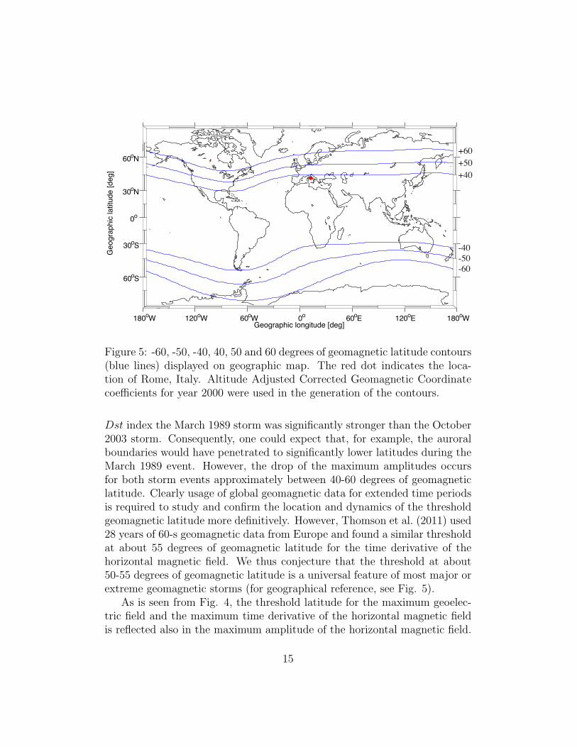
Figure 5: -60, -50, -40, 40, 50 and 60 degrees of geomagnetic latitude contours(blue lines) displayed on geographic map. The red dot indicates the loca-tion of Rome, Italy. Altitude Adjusted Corrected Geomagnetic Coordinatecoefficients for year 2000 were used in the generation of the contours.

Dst index the March 1989 storm was significantly stronger than the October2003 storm. Consequently, one could expect that, for example, the auroralboundaries would have penetrated to significantly lower latitudes during theMarch 1989 event. However, the drop of the maximum amplitudes occursfor both storm events approximately between 40-60 degrees of geomagneticlatitude. Clearly usage of global geomagnetic data for extended time periodsis required to study and confirm the location and dynamics of the thresholdgeomagnetic latitude more definitively. However, Thomson et al. (2011) used28 years of 60-s geomagnetic data from Europe and found a similar thresholdat about 55 degrees of geomagnetic latitude for the time derivative of thehorizontal magnetic field. We thus conjecture that the threshold at about50-55 degrees of geomagnetic latitude is a universal feature of most major orextreme geomagnetic storms (for geographical reference, see Fig. 5).

As is seen from Fig. 4, the threshold latitude for the maximum geoelec-tric field and the maximum time derivative of the horizontal magnetic fieldis reflected also in the maximum amplitude of the horizontal magnetic field.

15

This is an indication that the most extreme magnetic field fluctuations andgeoelectric field magnitudes are associated with the auroral current systemthat is known to be responsible for the largest perturbations of the groundmagnetic field. For example, while magnetospheric ring current can gener-ate horizontal magnetic field perturbations of the order of hundreds of nT,auroral currents regularly generate perturbations of the order thousands ofnT. Consequently, the question about the location of the threshold geomag-netic latitude can be cast also in terms of maximum possible expansion ofthe auroral current system.

Possibly the strongest geomagnetic storm in the recorded history is theCarrington event of September 1-2, 1859 (e.g., Tsurutani et al., 2003; Siscoeet al., 2006). The minimum estimated Dst index of the storm was -850 nTand there were (poleward horizon) auroral sightings from as low as 23 de-grees of geomagnetic latitude. However, from the viewpoint of the analysis inthis paper, perhaps the most significant observation during the event comesfrom Rome, Italy (see Fig. 5). More specifically, perturbation of the orderof 3000 nT was observed using a bifilar magnetometer that indicates rela-tive changes in the horizontal magnetic field strength (Loomis, 1860). Thegeomagnetic latitude of Rome, Italy is about 36 degrees and comparing thisto Figs. 4e and 4f, the observation indicates that the maximum expansionof the auroral current system may have been about 20 degrees more south-ward than during the March 1989 or October 2003 storms. Although thismay sound somewhat fantastic and the single data point was not based onmodern scientific instrumentation, one cannot simply disregard the Rome ob-servation. It may thus be possible that during the most extreme geomagneticstorms the auroral current system and the accompanying extreme geoelectricfields and GIC can penetrate significantly below the threshold at about 50degrees of geomagnetic latitude discussed above. Unfortunately, due to thepoor spatial coverage, low temporal sampling rates and off-scale magnitudes,magnetic recordings of the Carrington event do not allow for more detailedanalysis of the global geoelectric field and GIC characteristics (Nevanlinna,2006; Boteler, 2006; Nevanlinna, 2008). At sub-auroral latitudes in Finlandand Russia, the greatest measured hourly point deviations in the horizontalfield during the event were about 1000 nT (Nevanlinna, 2008).

Observations of low-latitude boundary of the auroral emissions indica-tive of the general location of the auroral region provide an alternative viewto question about of the threshold geomagnetic latitude. Records of auroralsightings are available also for historical storms and these enable approximate

16

reconstructions of the auroral region morphology during the correspondingstorms. For example, Silverman and Cliver (2001); Cliver and Svalgaard(2004); Silverman (2006) provide auroral data collected from numerous cat-alogues and earlier studies. Most importantly, Silverman and Cliver (2001)provide maximum equatorward extent of the visual aurora for three histor-ical extreme geomagnetic storms: August 28-29, 1859, September 1-2, 1859and May 14-15, 1921. While August 28-29, 1859 event was part of theAugust-September 1859 extreme storm sequence, analysis by Kappenman(2006) indicated that minimum Dst index of the May 14-15, 1921 event mayhave been comparable to that of the Carrington event. Silverman and Cliver(2001) provide auroral boundary locations both for the overhead auroras andauroras observed in the poleward horizon. However, only the overhead au-roral sightings provide unambiguous determination of the auroral boundarylocation and thus auroras observed in the poleward horizon are not discussedfurther here.

Table 1 shows the approximate low-latitude auroral boundary locationsfor the four extreme storm event. The boundary location for the March 13-15, 1989 was determined by visual inspection of Dynamic Explorer 1 (DE-1)ultraviolet auroral emission imaging data in Allen et al. (1989) for March 14,1989 01:51 UT. The visually determined boundary at about 40 degrees ofgeomagnetic latitude is in a very good agreement with the electron precip-itation boundary determined from low-Earth orbit Defense MeteorologicalSatellite Program (DMSP) satellite data by Yokoyama et al. (1998).

Table 1: The approximate maximum equatorward auroral boundary loca-tions of selected extreme geomagnetic storm events. The table is basedon data in Allen et al. (1989); Yokoyama et al. (1998); Silverman andCliver (2001). aMaximum equatorward extent of the overhead visual aurora.bMaximum equatorward extent in DE-1 imagery and electron precipitationboundary from DMSP.

Event Date Location in geomagnetic latitude

August 28-29, 1859 48 dega

September 1-2, 1859 41 dega

May 14-15, 1921 40 dega

March 13-15, 1989 40 degb

The striking feature of the data in Table 1 is that the boundary is confined

17

to approximately 40 degrees of geomagnetic latitude or greater for all fourevents. This is also the approximate low-latitude boundary for the transi-tion from low-latitude maximum field magnitudes to high-latitude maximumfield magnitudes seen in Fig. 4. As auroral emissions are congruent withthe auroral ionospheric current fluctuations, low-latitude auroral boundarylocations for extreme storm events in Table 1 along with “calibration” tomodern magnetic field observations via March 13-15 1989 event in Fig. 4provide further indication of possible generality of the threshold at about 50degrees of geomagnetic latitude. Although their results were based on dataonly for year 1998, Ahn et al. (2005) also concluded that the lowest possiblelatitude of the center of the ionospheric westward electrojet seems to be ataround 60 degrees of geomagnetic latitude, which is consistent with Figs. 3and 4. Ahn et al. (2005) also showed that the low-latitude boundary of auro-ral emissions tends to locate equatorward of the westward electrojet, whichis also consistent with our findings above.

It is noted that the Rome of observation of geomagnetic field perturbationof the order of 3000 nT during the Carrington event contradicts with theidea of the threshold geomagnetic latitude at about 50 degrees given the40 degrees of geomagnetic latitude boundary for the event in Table 1. Thepossible explanations for the discrepancy are 1) low-latitude boundary of theauroral emissions is not always congruent with the low-latitude boundary ofthe auroral ionospheric currents, 2) the actual low-latitude boundary of theoverhead auroral emissions was at the time of the Rome observation lowerthan 40 degrees of geomagnetic latitude but was not captured by any of thehistorical records and 3) the Rome magnetic field observation was erroneous.Although especially possibility 1) seems unlikely, further work is needed tofind the most plausible explanation for the discrepancy.

Although the Rome geomagnetic field recordings for the Carrington eventindicate that it may be possible for the auroral current system to penetratesignificantly lower than to about 50 degrees of the geomagnetic latitude, thereis no direct means to quantify the likelihood of such occurrence. Further, theapproximate low-latitude auroral boundary locations for some historical ex-treme events provide indication of maximum expansion of the auroral regionto about 40 degrees of geomagnetic latitude, which is consistent with theview in Figs. 3 and 4. Consequently, given the very similar properties ofthe March 1989 and October 2003 storms in Figs. 3 and 4 along with statis-tics by Thomson et al. (2011), we are inclined to hold our conjecture thatthe threshold at about 50-55 degrees of geomagnetic latitude holds for most

18

major and extreme geomagnetic storms - possibly also for 100-year events.In terms of extreme event scenarios and scaling this means that the extremegeoelectric field amplitudes experience about factor of 10 drop across the re-gion from 60 to 40 degrees of geomagnetic latitude (see Fig. 5). However, itis emphasized again that more extreme geomagnetic storm data is requiredfor more definite conclusions regarding the 100-year location of the thresholdgeomagnetic latitude.

2.4 Temporal scales of the extreme events

Many different types of dynamical processes in the solar wind-magnetosphere-ionosphere system are capable of generating large GIC. For example, auro-ral substorms, geomagnetic pulsations, sudden impulses and enhancementsof magnetospheric convection-related auroral electrojets are known to driveGIC (e.g., Kappenman, 2003; Pulkkinen et al., 2003; Viljanen et al., 2006b).All of these processes have their distinct spectral characteristics and thus nosingle simple synthetic temporal profile is capable of capturing the full tempo-ral variability observed during extreme storms (e.g., Pulkkinen and Kataoka,2006; Kataoka and Pulkkinen, 2008). Consequently, we chose to use actualgeomagnetic storm event to provide a representative temporal profile for thegenerated scenarios. We selected 10-s geomagnetic field observations fromNurmijarvi Geophysical Observatory, Finland and Memanbetsu GeophysicalObservatory, Japan for the period of October 29-31, 2003 to provide the tem-poral profiles for the scenarios. The Nurmijarvi Geophysical Observatory islocated approximately at 57 degrees of geomagnetic latitude and was thuswithin the region experiencing the most extreme magnetic field fluctuationsabove the threshold geomagnetic latitude during the storm. MemanbetsuGeophysical Observatory in turn is located approximately at 35 degrees of ge-omagnetic latitude and was thus within the region experiencing the magneticfield fluctuations below the threshold geomagnetic latitude during the storm.We also confirmed that the selected representative storm profiles include sig-natures of auroral substorms, geomagnetic pulsations, sudden impulses andenhancements of magnetospheric convection-related auroral electrojets. Theselected magnetometer stations and the geomagnetic storm event thus pro-vide a good representation of the ground electromagnetic field fluctuationsduring major geomagnetic storms.

Geomagnetic field observations from Nurmijarvi and Memanbetsu Geo-physical Observatories for October 29-31, 2003 where applied with the Que-

19

bec ground conductivity model and the plane wave method to map the geo-magnetic field into the horizontal geoelectric field. The obtained geoelectricfield time series was then normalized so that the maximum amplitude of thesignal is exactly 1 (Fig. 6), i.e.

max(√E2

x + E2y) = 1 (3)

where Ex and Ey are the normalized horizontal geoelectric field componentsand the maximum is taken over the storm event. The normalized horizontalgeoelectric field is the signal that is used to scale to different maximum 100-year amplitude scenarios as a function of ground conductivity structures andgeomagnetic latitudes.

2.5 Spatial scales of the extreme events

In the challenge of generating 100-year geoelectric field and GIC scenarios,characterizing the spatial scales of the extreme events may the most difficulttask. As was discussed above, many different types of processes in the so-lar wind-magnetosphere-ionosphere system drive large GIC and each of theseprocesses have their characteristic temporal and spatial scales. Especially theglobal spatial scales of the geoelectric field associated with these processesare generally not well-known. However, high-latitude (auroral) magneticfield and geoelectric field fluctuations tend to be often poorly correlated overdistances larger than of the order of 100 km (Pulkkinen et al., 2007, andreferences therein). Since on the other hand the extreme geomagnetic fieldand geoelectric field fluctuations are associated with the enhancements ofthe auroral current system that can be global, these two aspects give rise toa two-fold view: while large or extreme geoelectric field magnitudes can beexperienced across the globe in the region covered by the auroral current sys-tem, the spatial correlation lengths associated with the field fluctuations canbe short. Further complications are caused by the horizontal variations inthe ground conductivity structure. The electromagnetic response to geospacedriving is a strong function of the ground conductivity structure and steephorizontal conductivity gradients can generate steep fluctuations in the spa-tial geoelectric field structure.

Since we have no means of generating a global geoelectric field structurethat would represent with any reasonable accuracy the true spatial scales(and spatial correlations) of the extreme fields, we are constrained to rep-

20

a)

0 10 20 30 40 50 60 70−0.5

0

0.5

1

UT [hours]

EX [n

orm

aliz

ed a

mpl

itude

]

Normalized representative super−threshold storm event (geoelectric field)

0 10 20 30 40 50 60 70−1

−0.5

0

0.5

1

UT [hours]

EY [n

orm

aliz

ed a

mpl

itude

]

44.5 45 45.5 46−0.5

0

0.5

1

UT [hours]

EX [n

orm

aliz

ed a

mpl

itude

]

Normalized representative super−threshold storm event (geoelectric field)

44.5 45 45.5 46−1

−0.5

0

0.5

1

UT [hours]

EY [n

orm

aliz

ed a

mpl

itude

]

0 10 20 30 40 50 60 70−1

−0.5

0

0.5

1

UT [hours]

EX [n

orm

aliz

ed a

mpl

itude

]

Normalized representative sub−threshold storm event (geoelectric field)

0 10 20 30 40 50 60 70−1

−0.5

0

0.5

UT [hours]

EY [n

orm

aliz

ed a

mpl

itude

]

6 6.5 7 7.5−1

−0.5

0

0.5

1

UT [hours]

EX [n

orm

aliz

ed a

mpl

itude

]

Normalized representative sub−threshold storm event (geoelectric field)

6 6.5 7 7.5−1

−0.5

0

0.5

UT [hours]

EY [n

orm

aliz

ed a

mpl

itude

]

b)

Figure 6: Normalized representative horizontal geoelectric field components(X indicates geographic north, Y indicates geographic east) for the full stormevent and 1.5 hour long subsection containing the maximum field magnitudefor super-threshold geomagnetic latitude locations represented by NurmijarviGeophysical Observatory (panel a) and sub-threshold geomagnetic latitudelocations represented by Memanbetsu Geophysical Observatory (panel b).The time is hours from October 29, 2003 00:00 UT. The maximum geoelectricfield magnitude at Nurmijarvi was caused by an auroral substorm while themaximum field magnitude at Memanbetsu was caused by a sudden impulse.See the text for details.

21

resent fields in regional scales. Consequently, we will assume that the geo-electric field is uniform over spatial scales of the order of 100-1000 km. Inanother words, the geoelectric field of the extreme storm scenarios has thesame instantaneous direction and magnitude throughout the region of inter-est. The spatial uniformity amounts to assuming that there are no significanthorizontal variations in the ground conductivity structure or in the spatialstructure of the source field fluctuations. It is emphasized that while theseassumptions may be reasonable for the purpose of the extreme scenarios onregional scales, they will break and should not be used in global scales.

3 Summary of the extreme geoelectric field

scenarios

Summarizing the findings in Section 2, the four key factors introduced inSection 1 are addressed in the extreme geoelectric field scenarios the followingways:

• The effect of the ground conductivity structure on the extreme geo-electric field amplitudes - two ground conductivity models representingrealistic extreme ends of conducting and resistive grounds were appliedwith the IMAGE magnetometer data and the plane wave method. Theresults were used to estimate 100-year amplitudes of the 10 secondresolution horizontal geoelectric field at high-latitudes. The resistiveground model is associated with approximately factor of five largergeoelectric field amplitudes than the conducting ground model.

• The effect of the geomagnetic latitude on the extreme geoelectric fieldamplitudes - we identified a threshold geomagnetic latitude across whichthe maximum geoelectric field amplitudes experience approximately anorder of magnitude decrease.

• Temporal scales of the extreme events - representative time series fromselected magnetometer stations for a major event storm event wereused to provide realistic temporal profiles. Stations above and belowthe identified threshold geomagnetic latitude are used.

• Spatial scales of the extreme events - we assume spatially uniform geo-electric field structure in regional scales.

22

Fig. 7 summarizes the generated four 100-year geoelectric field scenarios.In Fig. 7a and Fig. 7b the normalized geoelectric field in Fig. 6a wasscaled using the maximum amplitudes of 20 V/km and 5 V/km obtainedfrom the high-latitude statistics in Fig. 1. In Fig. 7c and Fig. 7d thenormalized geoelectric field in Fig. 6b was scaled by order of magnitudesmaller maximum field strengths for sub-threshold geomagnetic latitudes.The threshold geomagnetic latitude can be set to 50 degrees or for moreconservative estimates to 40 degrees of geomagnetic latitude. The geoelectricfield is assumed spatially uniform in regional scales for all scenarios in Fig.7.

4 Mapping geoelectric field scenario to geo-

magnetically induced currents

Mapping the extreme geoelectric field scenarios into GIC is a highly system-dependent operation. The response of the conductor system is dependent onthe electrical characteristics and topology of the system and consequently it isgenerally speaking not feasible to provide any “prototype” configuration thatcould be applied to a variety of different situations. In another words, oneneeds to have additional engineering information available about the char-acteristics of the conductor system of interest prior to mapping geoelectricfield into GIC.

Once the engineering information about the system has been acquired,there are two fairly straightforward means to carry out the mapping. First, ifcomputation of GIC distribution throughout the (regional) system is needed,one can apply techniques by Lehtinen and Pirjola (1985) for discretely groundedsystems such as high voltage transmission systems and so-called distributedsource transmission line (DSTL) theory for continuously grounded systemssuch as buried oil and gas pipelines (Boteler, 1997).

To demonstrate the application of the extreme geoelectric field scenariosin computing GIC distribution throughout a high-voltage power transmissionsystem, we considered Dominion’s Virginia Power grid model shown in Fig.8. The model is built based on a DC-mapping of Dominion’s high-voltagetransmission network. Typically, due to the scales associated with the GICphenomenon, DC models should contemplate the 500 kV and the 230 kVnetworks; a few key 115 kV transmission lines are also considered in this

23

0 10 20 30 40 50 60 70−10

−5

0

5

10

15

UT [hours]

EX [V

/km

]

Extreme super−threshold geoelectric field scenario. Scenario max(|E|): 20.0 V/km.

0 10 20 30 40 50 60 70−20

−10

0

10

20

UT [hours]

EY [V

/km

]

0 10 20 30 40 50 60 70−2

−1

0

1

2

3

4

UT [hours]

EX [V

/km

]

Extreme super−threshold geoelectric field scenario. Scenario max(|E|): 5.0 V/km.

0 10 20 30 40 50 60 70−4

−2

0

2

4

UT [hours]

EY [V

/km

]

0 10 20 30 40 50 60 70−2

−1

0

1

2

UT [hours]

EX [V

/km

]

Extreme sub−threshold geoelectric field scenario. Scenario max(|E|): 2.0 V/km.

0 10 20 30 40 50 60 70−2

−1.5

−1

−0.5

0

0.5

1

UT [hours]

EY [V

/km

]

0 10 20 30 40 50 60 70−0.4

−0.2

0

0.2

0.4

UT [hours]

EX [V

/km

]Extreme sub−threshold geoelectric field scenario. Scenario max(|E|): 0.5 V/km.

0 10 20 30 40 50 60 70−0.6

−0.4

−0.2

0

0.2

UT [hours]

EY [V

/km

]

Above threshold geo-magnetic latitude

Below threshold geo-magnetic latitude

Resistive ground Conducting grounda) b)

c) d)

Figure 7: Illustration of extreme horizontal geoelectric field scenarios (Xindicates geographic north, Y indicates geographic east). Panel a): Scenariofor resistive ground structures for locations above the threshold geomagneticlatitude. The maximum geoelectric field amplitude is 20 V/km. Panel b):Scenario for conductive ground structures for locations above the thresholdgeomagnetic latitude. The maximum geoelectric field amplitude is 5 V/km.Panel c): Scenario for resistive ground structures for locations below thethreshold geomagnetic latitude. The maximum geoelectric field amplitude is2 V/km. Panel a): Scenario for conductive ground structures for locationsbelow the threshold geomagnetic latitude. The maximum geoelectric fieldamplitude is 0.5 V/km. Note that the vertical scales are different in differentpanels.

24

particular model. Since the geoelectric field is assumed spatially uniformacross the system, transmission lines between substations can be representedas straight lines. At each system inter-tie, a system equivalent is modeled asa low resistance to the ground (0.1 Ω).

The calculation of GIC flows in Dominion’s high-voltage transmission sys-tem is performed by using the matrix formulation derived in Lehtinen andPirjola (1985). In general, GIC flows are a function of system topology, lineresistances and geospatial orientation, transformer type and winding resis-tance, grounding resistance, series line compensation, and of course, geoelec-tric field. Fig. 8 shows a snapshot of GIC flows at each substation, in aper-phase basis, caused by the maximum amplitude of the geoelectric field inthe scenario shown in Fig. 7c. The selection of the storm scenario is based onDominion’s geomagnetic latitude (below the threshold latitude) and groundconductivity (resistive ground). To demonstrate that the approach providesa time series of GIC throughout the system over the entire storm scenario,Fig. 9 shows times series of modeled GIC flow in one of Dominion’s trans-formers. Note that the approach provides corresponding time series for anylocation in the high-voltage transmission system.

In an alternative approach, if only local GIC flowing through, for example,individual node of power transmission system is needed, one can apply simplelinear relation

GIC = aEx + bEy (4)

where (Ex, Ey) are the horizontal components of the geoelectric field and(a, b) the system parameters. (a, b) that depend on the topology and electricalcharacteristics of the conductor system under investigation can be derivedfor individual locations by using information about the full conductor system(Pulkkinen et al., 2006) or by inverting the parameters from GIC and groundmagnetic field observations (Pulkkinen et al., 2007). The linear relation inEq. (4) has been shown in numerous studies to hold to a good approximationin many situations of interest (e.g., Pulkkinen et al., 2006; Ngwira et al., 2008;Pulkkinen et al., 2010). The typical values for (a, b) are in the range between0-200 A·km/V (Pulkkinen et al., 2008, and references therein). For example,using mid-range a = b = 50 A·km/V one gets the extreme GIC scenario inFig. 10 for conductive ground at location above the threshold geomagneticlatitude.

25

!

2 V/km

Figure 8: Modeled GIC distribution in the Dominion’s Virginia Power high-voltage transmission system for hour 6.17 in the scenario shown in Fig. 7c.Green, blue and red lines indicate 500 kV, 230 kV and 115 kV transmissionlines, respectively. The back arrow indicates the direction and magnitude ofthe horizontal geoelectric field and blue and red circles indicate the magni-tude of GIC flowing from the ground to the grid and from the grid to theground, respectively. For auto-transformers, an effective GIC value is used(Albertson, 1981). System equivalents, i.e. inter-ties to other systems, arerepresented by squares.

26

Figure 9: Time series of the modeled GIC in one of Dominion’s VirginiaPower high-voltage transmission system transformers for the extreme geo-electric field scenario in Fig. 7c. The configuration of the transmissionsystem is shown in Fig. 8. Only maximum amplitude GIC taken over 10minute windows are shown.

0 10 20 30 40 50 60 70−300

−200

−100

0

100

200

300

400

UT [hours]

GIC

[A]

Extreme GIC scenario.

Figure 10: Extreme GIC scenario for conductive ground at location abovethe threshold geomagnetic latitude. System parameters a = b = 50 A·km/Vwhere used to map the geoelectric field into GIC. See the text for details.

27

5 Discussion

In this paper we explored 100-year extreme geoelectric field scenarios bytaking into account the key geophysical factors associated with the geomag-netic induction process. More specifically, we derived explicit geoelectricfield temporal profiles as a function of ground conductivity structures andgeomagnetic latitudes. We also demonstrated how the extreme geoelectricfield scenarios can be mapped into GIC. The computed GIC can then be usein further engineering analyses that are needed to quantify the impact onthe conductor systems such as high-voltage power transmission systems ofinterest.

Although we hope that the work in this paper provides initial input forfurther engineering analyses attempting to quantify the impact of extremegeomagnetic storms on high-voltage power transmission systems, it is em-phasized that further work is needed to refine and improve the generatedscenarios. For example, due to the poor knowledge of global spatial charac-teristics of the geoelectric field during extreme events, the scenarios presentedin this paper apply only to regional scales of the order of 100-1000 km. Itis of great interest to expand the scenarios for application in direct globalcalculations.

Also, one-dimensional representative ground conductivity models wereused to account for varying electromagnetic response of different local geo-logical structures. In principle, if the local ground conductivity is known,the statistics used in this paper can be tailored for specific regions providingthus significant refinement for extreme geoelectric field scenarios. It is alsoof interest to investigate the impact of steep horizontal ground conductiv-ity gradients on the extreme geoelectric field scenarios. For this one wouldneed to utilize more complex mathematical framework allowing two- or three-dimensional ground conductivity structures in the calculation of the geoelec-tric field. We, however, emphasize that effective one-dimensional groundconductivity models applied with the plane wave method are reasonable inmany, if not in most, situations.

Perhaps the most critical and still somewhat open question that needsfurther clarification concerns the dynamics and the location of the identi-fied threshold geomagnetic latitude. Since the geoelectric field amplitudesexperience significant drop across the threshold, the location has significantimplications for the extension of global impacts of extreme storms. Detailedstudies of the historical records of extreme geomagnetic storms and accom-

28

panied auroral sightings as well as physics-based magnetosphere-ionospheremodels capturing the key physical processes associated with the low-latitudeauroral boundary may be used to shed further light on the topic.

Ultimately, only the high temporal resolution global geomagnetic record-ings for very extended time periods are able to provide definitive quantifica-tion of likelihoods and spatiotemporal characterization of extreme geomag-netic storm events. The modern 60-s digital recordings are available onlysince about 1980s, which presents obvious difficulties in trying to extract in-formation about 100-year events today. Regular refinement of the statisticsderived in this paper should thus be carried out and over time we will be ableto quantify more definitively the severity of 100-year geomagnetic storms.

Since the major of the goal of the work at hand is to facilitate furtherengineering analyses quantifying the extreme geomagnetic storm impact onhigh-voltage transmission systems, the generated extreme geoelectric fieldscenarios in Fig. 7 are publicly available. The digital data can be requestedfrom A. Pulkkinen (antti.a.pulkkinen@nasa.gov).

Appendix A: Mapping the ground geomagnetic

field into the geoelectric field

Because of the central role of the process in most GIC modeling, we give herea brief overview of application of the plane wave method to mapping of theground geomagnetic field fluctuations into the geoelectric field. The methodwas first formulated by Cagniard (1953) and has since been used extensivelyin general geomagnetic induction and magnetotelluric studies. The methodis based on the concept of surface impedance, which is defined as

Z = µ0Ex

By

= −µ0Ey

Bx

(5)

where (Ex, Ey) and (Bx, By) are the horizontal components of the electricfield and magnetic field, respectively, µ0 is the vacuum permeability andtilde indicates quantities in the spectral domain. In geophysical applicationsof Eq. (5) the fields are evaluated at the surface of the Earth. By assumingquasi-static temporal fluctuations, i.e. neglecting the displacement currentin Maxwell’s equations, and by assuming that the horizontal field gradients

29

vanish, the impedance of the layer n of one-dimensional layered ground canbe computed using recursive formula

Zn =iωµ0

γn

coth(γndn + coth−1(γn

iωµ0

Zn+1)) (6)

where γ2n = iωµ0σn, dn the thickness of the layer n, ω the angular frequency

of the field fluctuations and σn is the conductivity of the layer n. To obtainthe surface impedance in Eq. (5), one sets n = 1 in Eq. (6) and computesthe impedance values recursively starting from the bottom of the modeledground structure. The bottom layer is assumed infinitely thick.

While quasi-stationary approximation is valid for geomagnetic inductionstudies having typically frequencies of temporal field fluctuations below 1 Hz(e.g., Weaver, 1994), the assumption about vanishing horizontal gradients offield fluctuations may seem at first invalid especially during strong geomag-netic storm conditions. However, Dmitriev and Berdichevsky (1979) showedthat the above formulation holds also if the plane wave requirement is relaxedinto assumption about locally (∼ 100 km) linear variation of the surface mag-netic field. The extended validity of the “plane wave” formulation is likelyone key reason for the success of the method in GIC applications.

The process for mapping the ground geomagnetic field into the geoelectricfield is then as follows:

1. Convert the horizontal ground geomagnetic field into the spectral do-main by using the Fourier transform.

2. Compute the surface impedance using Eq. (6).

3. Compute the spectral domain horizontal geoelectric field using Eq. (5).

4. Convert the spectral domain geoelectric field into the time domain usingthe inverse Fourier transform.

It is also noted that it follows from the basic properties of the Fouriertransform:

B =1

iω

dB

dt(ω) (7)

Consequently, computation of the geoelectric field from both the groundgeomagnetic field and the time derivative of the geomagnetic field using Eqs.(5) and (6) is a linear operation.

30

Acknowledgements

This work was carried out in connection with the North American ElectricReliability Corporation Geomagnetic Disturbances Task Force (GMDTF)activity taking place during year 2011. The valuable feedback from theGMDTF community helped greatly to shape our work and to make the all im-portant connection between the geophysics and power engineering sides of theGIC problem. We acknowledge especially Mr. R. Lordan (Electric Power Re-search Institute), Mr. D. Watkins (Bonneville Power Administration), Drs.Luis Marti (Hydro One), M. Hesse (NASA Goddard Space Flight Center),H. Nevanlinna (Finnish Meteorological Institute), A. Thomson (British Ge-ological Survey), A. Viljanen (Finnish Meteorological Institute), R. Pirjola(Finnish Meteorological Institute) and R. Kataoka (Tokyo Institute of Tech-nology) for fruitful discussions and comments that substantially enhanced thequality of our work. Dr. Y. Zheng (NASA Goddard Space Flight Center) isacknowledged for help with the study of the location of auroral boundariesduring the March 1989 event. The results presented in this paper rely ondata collected at magnetic observatories. We thank the national institutesthat support them and INTERMAGNET for promoting high standards ofmagnetic observatory practice (www.intermagnet.org). The Dst index datawas provided by the World Data Center for Geomagnetism, Kyoto, Japan.We thank the institutes who maintain the IMAGE Magnetometer Array thatprovided the data used in deriving the geoelectric field statistics of the work.Dr. A. Viljanen is acknowledged for providing Nurmijarvi Geophysical Ob-servatory data. Geomagnetic field data at Memanbetsu station is provided byKakioka Magnetic Observatory, Japan Meteorological Agency (KMO-JMA).

31

References

Ahn, B.-H., G. X. Chen, W. Sun, J. W. Gjerloev, Y. Kamide, J. B. Sig-warth, and L. A. Frank, Equatorward expansion of the westward electro-jet during magnetically disturbed periods, J. Geophys. Res., 110, A01305,doi:10.1029/2004JA010553, 2005.

Albertson, V.D., Load-Flow Studies in the Presence of Geomagnetically-Induced Currents, IEEE Transactions on Power Apparatus and Systems,Vol. PAS-100, No. 2, February 1981.

Allen, J., H. Sauer, L. Frank, and P. Reiff, Effects of the March 1989 SolarActivity, EOS, Vol. 70, No. 46, November 14, 1989.

Berdichevsky, M., and M. Zhdanov, Advanced theory of deep geomagneticsounding, Elsevier Science Publishers B.V., Netherlands, 408 pp., 1984.

Borovsky, J. E., and M. H. Denton, Differences between CME- drivenstorms and CIR-driven storms, J. Geophys. Res., 111, A07S08,doi:10.1029/2005JA011447, 2006.

Boteler, D. H., Assessment of geomagnetic hazard to power systems inCanada, Nat. Hazards, 23, 101-120, 2001.

Boteler, D. H., The super storms of August/September 1859 and their effectson the telegraph system, Adv. Space Res., 38, 159-172, 2006.

Dmitriev, V., and M. Berdichevsky, The fundamental model of magnetotel-luric sounding, IEEE Proc., 67, 1034, 1979.

Bolduc, L., GIC observations and studies in the Hydro-Quebec power system,J. Atmos. Sol.-Terr. Phys., 64, 1793-1802, 2002.

Boteler, D., Distributed source transmission line theory for electromagneticinduction studies, Supplement of the Proceedings of the 12th InternationalZurich Symposium and Technical Exhibition on Electromagnetic Compat-ibility, 401 408, 1997.

Cagniard, L., Basic theory of the magneto-telluric method of geophysicalprospecting, Geophysics, 18, 605, 1953.

32

Campbell, W. C. (1980), Observation of electric currents in the Alaska oilpipeline resulting from auroral electrojet current sources, Geophys. J. R.Astron. Soc., 61, 437-449, 1980.

Cliver, E.W., and L. Svalgaard, The 1859 solarterrestrial disturbance andthe current limits of extreme space weather activity, Solar Physics, 224,407-422, 2004.

Gaunt, C.T., and G. Coetzee, Transformer failures in regions incorrectlyconsidered to have low GIC-risk, In: Proceedings of Power Tech, July 15,2007, Lausanne, Switzerland.

Grossi, P., and H. Kunreuther (eds.), Catastrophe Modeling: A New Ap-proach to Managing Risk, Springer, 2005.

Huttunen, K. E. J., S. P. Kilpua, A. Pulkkinen, A. Viljanen, and E. Tanska-nen, Solar wind drivers of large geomagnetically induced currents duringthe solar cycle 23, Space Weather, 6, S10002, doi:10.1029/2007SW000374,2008.

Kappenman, J.G., Geomagnetic Storms and Their Impact on Power Systems,IEEE Power Eng. Rev., May 1996, 5, 1996.

Kappenman, J. G., Storm sudden commencement events and the asso-ciated geomagnetically induced current risks to ground-based systemsat low-latitude and midlatitude locations, Space Weather, 1(3), 1016,doi:10.1029/2003SW000009, 2003.

Kappenman, J.G., Great geomagnetic storms and extreme impulsive geo-magnetic field disturbance events An analysis of observational evidenceincluding the great storm of May 1921, Advances in Space Research, 38,188199, 2006.

Kataoka, R., and A. Pulkkinen, Geomagnetically induced currents dur-ing intense storms driven by coronal mass ejections and corotatinginteracting regions, Journal of Geophysical Research, 113, A03S12,doi:10.1029/2007JA012487, 2008.

Langlois, P., L. Bolduc, and M. C. Chouteau, Probability of occurrence ofgeomagnetic storms based on a study of the distribu- tion of the electric

33

field amplitudes measured in Abitibi, Quebec, in 1993-94, J. Geomagn.Geoelectr., 48, 1033-1041, 1996.

Lehtinen, M., and R. Pirjola, Currents produced in earthed conductor net-works by geomagnetically-induced electric fields, Ann. Geophys., 3, 4, 479-484, 1985.

Loomis, E, The great auroral exhibition of Aug. 28th to Sept. 4th, 1859. 4thArticle, American Journal of Science, 79, 386399, 1860.

Luhr, H., S. Maus, and M. Rother, Noon-time equatorial electrojet: Itsspatial features as determined by the CHAMP satellite, J. Geophys. Res.,109, A01306, doi:10.1029/2002JA009656, 2004.

Molinski, T., Why utilities respect geomagnetically induced currents, Journalof Atmospheric and Solar-Terrestrial Physics, 64, 17651778, 2002.

Muir-Wood, R., and P. Grossi, The catastrophe modeling response to Hur-ricane Katrina, in Climate Extremes and Society by Henry F. Diaz andRichard J. Murnane (eds.), Cambridge University Press, 356 pp., 2008.

National Research Council, Severe Space Weather Events-UnderstandingSocietal and Economic Impacts: A Workshop Report, The NationalAcademies Press, Washington, DC, 2008.

North American Electric Reliability Corporation and the US Department ofEnergy, High-Impact, Low-Frequency Event Risk to the North AmericanBulk Power System, Report of the November 2009 Workshop, June 2010.

Nevanlinna, H., A study on the great geomagnetic storm of 1859: Compar-isons with other storms in the 19th century, Adv. Space Res., 38, 180-187,2006.

Nevanlinna, H., On geomagnetic variations during the August- Septemberstorms of 1859, Adv. Space Res., 42, 171-180, 2008.

Ngwira, C. M., A. Pulkkinen, L.-A. McKinnell, and P. J. Cilliers, Improvedmodeling of geomagnetically induced currents in the South African powernetwork, Space Weather, 6, S11004, doi:10.1029/2008SW000408, 2008.

34

Ohtani, S.-I., R. Fujii, M. Hesse, and R.L. Lysak (eds.), MagnetosphericCurrent Systems, GU Geophysical Monograph 118, American GeophysicalUnion, Washington, 2000.

Pulkkinen, A., A. Thomson, E. Clarke, and A. McKay, April 2000 geomag-netic storm: ionospheric drivers of large geomagnetically induced currents,Annales Geophysicae, 21, 709717, 2003.

Pulkkinen, A., S. Lindahl, A. Viljanen, and R. Pirjola, Geomagnetic storm of29-31 October 2003: Geomagnetically induced currents and their relationto problems in the Swedish high-voltage power transmission system, SpaceWeather, 3, S08C03, doi:10.1029/2004SW000123, 2005.

Pulkkinen, A., and R. Kataoka, S-transform view of geomagnetically inducedcurrents during geomagnetic superstorms, Geophys. Res. Lett., 33, L12108,doi:10.1029/2006GL025822, 2006.

Pulkkinen, A., A. Viljanen, and R. Pirjola, Estimation of geomagneticallyinduced current levels from different input data, Space Weather, 4, S08005,doi:10.1029/2006SW000229, 2006.

Pulkkinen, A., Spatiotemporal characteristics of the ground electromagneticfield fluctuations in the auroral region and implications on the predictabil-ity of geomagnetically induced currents, in Space Weather, Research to-wards Applications in Europe, Series: Astrophysics and Space Science Li-brary, Vol. 344, 2007, XII, 332 p., Springer, 2007.

Pulkkinen, A., R. Pirjola, and A. Viljanen, Determination of ground con-ductivity and system parameters for optimal modeling of geomagneticallyinduced current flow in technological systems, Earth Planets Space, 59,9991006, 2007.

Pulkkinen, A., R. Pirjola, and A. Viljanen, Statistics of extreme ge-omagnetically induced current events, Space Weather, 6, S07001,doi:10.1029/2008SW000388, 2008.

Pulkkinen, A., R. Kataoka, S. Watari, and M. Ichiki, Modeling geomagnet-ically induced currents in Hokkaido, Japan, Advances in Space Research,46, 10871093, 2010.

35

Silverman, S.M., and E.W. Cliver, Low-latitude auroras: the magnetic stormof 1415 May 1921, Journal of Atmospheric and Solar-Terrestrial Physics,63, 523535, 2001.

Silverman, S.M., Comparison of the aurora of September 1/2, 1859 withother great auroras, Advances in Space Research, 38, 136144, 2006.

Siscoe, G., N.U. Crooker, and C.R. Clauer, Dst of the Carrington storm of1859, Advances in Space Research, 38, 173179, 2006.

Thomson, A. W. P., A. J. McKay, E. Clarke, and S. J. Reay, Surface electricfields and geomagnetically induced currents in the Scottish Power gridduring the 30 October 2003 geomagnetic storm, Space Weather, 3, S11002,doi:10.1029/2005SW000156, 2005.

Thomson, A., S. Reay, and E. Dawson, Quantifying Extreme Behaviour inGeomagnetic Activity, Space Weather, in press, 2011.

Trichtchenko, L., and D. Boteler, Modeling Geomagnetically Induced Cur-rents Using Geomagnetic Indices and Data, IEEE Transactions on PlasmaScience, Vol. 32, No. 4, August, 2004.

Tsubouchi, K., and Y. Omura, Long-term occurrence probabilitiesof intense geomagnetic storm events, Space Weather, 5, S12003,doi:10.1029/2007SW000329, 2007.

Tsurutani, B. T., W. D. Gonzalez, G. S. Lakhina, and S. Alex, The extrememagnetic storm of 12 September 1859, J. Geophys. Res., 108(A7), 1268,doi:10.1029/2002JA009504, 2003.

Viljanen, A., H. Nevanlinna, K. Pajunpaa, and A. Pulkkinen, Time deriva-tive of the horizontal geomagnetic field as an activity indicator, AnnalesGeophysicae, 19, 11071118, 2001.

Viljanen, A., A. Pulkkinen, R. Pirjola, K. Pajunpaa, P. Posio, and A. Koisti-nen, Recordings of geomagnetically induced currents and a nowcasting ser-vice of the Finnish natural gas pipeline system, Space Weather, 4, S10004,doi:10.1029/2006SW000234, 2006a.

Viljanen, A., E.I. Tanskanen, and A. Pulkkinen, Relation between substormcharacteristics and rapid temporal variations of the ground magnetic field,Ann. Geophys., 24, 725733, 2006.

36

Wait, J.R., Electromagnetic Waves in Stratified Media, 2nd Ed., PergamonPress, 608 pp., 1970.

Weaver, J.T., Mathematical Methods for Geo-electromagnetic Induction,John Wiley and Sons Inc., 316 pp., 1994.

Weigel, R.S., and D.N Baker, Probability distribution invariance of 1-minuteauroral-zone geomagnetic field fluctuations, Geophysical Research Letters,Vol. 30, No. 23, 2193, doi:10.1029/2003GL018470, 2003.

Wik, M., A. Viljanen, R. Pirjola, A. Pulkkinen, P. Wintoft, and H.Lundstedt, Calculation of geomagnetically induced currents in the400 kV power grid in southern Sweden, Space Weather, 6, S07005,doi:10.1029/2007SW000343, 2008.

Yokoyama, N., Y. Kamide, and H. Miyaoka, The size of auroral belt duringmagnetic storms, Annales Geophysicae, 16, 566-573, 1998.

37