Gasoline Prices, Transport Costs, and the U.S. Business

Cycles

Hakan Yilmazkuday�

June 1, 2014

Abstract

The e¤ects of gasoline prices on the U.S. business cycles are investigated. In order to

distinguish between gasoline supply and gasoline demand shocks, the price of gasoline is

endogenously determined through a transportation sector that uses gasoline as an input of

production. The model is estimated for the U.S. economy using �ve macroeconomic time

series, including data on transport costs and gasoline prices. The results show that although

standard shocks in the literature (e.g., technology shocks, monetary policy shocks) have sig-

ni�cant e¤ects on the U.S. business cycles in the long run, gasoline supply and demand shocks

play an important role in the short run.

JEL Classi�cation: E32, E52, F41

Key Words: Business Cycles, Transport Costs, Gasoline Prices

�Department of Economics, Florida International University, Miami, FL 33199, USA. Phone:305-348-2316. E-

mail: hakan.yilmazkuday@�u.edu

1. Introduction

There is a close relationship between gasoline prices and the business cycles. One reason is that

transportation of goods between producers and consumers is achieved by using gasoline as the main

input. A second reason is that gasoline is by far the most important form of energy consumed in

the United States; e.g., it accounts for 48.7% of all energy used by consumers.1 A third reason is

that gasoline prices re�ect the developments in the global energy markets.2 A fourth (and maybe

the most important) reason is that gasoline is the form of energy with the most volatile price,

which is important for any business cycle analysis.3

This paper investigates this relationship for the U.S. economy. In technical terms, the main

innovation in this paper is to include a transportation sector (that uses gasoline as an input of

production) between producers and consumers in an otherwise standard DSGE model. In the

model, we can distinguish between demand and supply shocks by assuming a given (exogenous)

endowment of gasoline, while letting the gasoline price to be determined in equilibrium. The

optimization of households and �rms results in an expression for the nominal price of gasoline

depending on future nominal gasoline prices, future gasoline supply shocks, and nominal interest

rates. The equilibrium real price of gasoline further depends on the global real economic activity

together with the global endowment of gasoline.

In equilibrium, the e¤ects of transport costs and gasoline prices are further summarized in an

IS equation, a Phillips curve, a terms of trade expression, a monetary policy rule, and real prices of

transportation and gasoline. Hence, in this paper, possible e¤ects of gasoline supply and demand

shocks on output, in�ation, and transport costs can be investigated together with the e¤ects of

other shocks accepted as standard in the literature. We pursue such an approach to investigate

the volatilities in gasoline prices and their e¤ects on the U.S. business cycles. The results show

that although standard shocks in the literature (e.g., technology shocks or monetary policy shocks)

have signi�cant e¤ects on the U.S. business cycles in the long run, gasoline supply and demand

shocks play an important role in the short run.4

Some earlier DSGE studies have also considered energy prices (mostly in the form of oil prices)

and their e¤ects on economic activity.5 In the recent literature, Dhawan and Jeske (2008) have

1See Kilian (2008); gasoline is followed by electricity with a share of 33.8% and natural gas with a share of 12.3%.2For example, crude oil is the main input into gasoline production.3A more detailed comparison between energy, oil, and gasoline prices has been provided in Kilian (2010)4See Kilian (2008) and Edelstein and Kilian (2009) for discussions on mechanisms that explain how consumption

expenditures may be directly a¤ected by energy price changes.5As earlier modeling approaches, see Hamilton (1988), Kim and Loungani (1992), Backus and Crucini (1992),

modeled (and calibrated) the energy consumption of households and �rms; however, they have

not endogenized the price of energy or estimated their model, hence they have not empirically

distinguished between energy supply and energy demand shocks in the U.S. economy. Although

Bodenstein et al. (2011) have endogenized energy prices and investigated (through calibrating) the

role of �nancial risk sharing in a two-country DSGE model of the external adjustments caused by

energy price shocks, they have not estimated their model and have not investigated the e¤ects of

energy shocks on the U.S. business cycles. Nakov and Pescatori (2010) have modeled and estimated

energy-market speci�c demand shocks through considering energy consumption of �rms, but they

have not considered the demand shocks through energy consumption of �nal consumers or through

the transportation sector. Balke et al. (2010) and Bodenstein and Guerrieri (2011) have modeled

and estimated the energy consumption of households and �rms; however, they have not considered

the role of energy shocks through modeling a transportation sector, either. In contrast, this paper

investigates all of these mentioned dimensions by modeling demand for and supply of gasoline

which is by far the most important form of energy consumed in the United States.

The rest of the paper is organized as follows. Section 2 introduces the economic environment.

Section 3 introduces the data and the estimation methodology. Section 4 depicts the estimation

results and discusses the robustness of the analysis. Section 5 concludes. The log-linearized version

of the model, together with its implications, is given in the Appendices.

2. Economic Environment

The two-country model is populated by a representative household, a continuum of production

�rms, a continuum of transportation �rms taking care of the transportation of goods from pro-

ducers to consumers, and a monetary authority.6 It is a continuum of goods model in which all

goods are tradable, the representative household holds assets, the production of goods requires

labor input (subject to a production technology), and the production of transportation services

requires gasoline input (subject to a transportation technology).

In terms of the notation, subscripts H and F stand for domestically and foreign-produced

goods, respectively; superscript � stands for the variables of the foreign country (i.e., rest of theworld).7

Rotemberg and Woodford (1996), and Finn (2000).6The model builds upon models such as Benigno and Benigno (2006) by introducing a transportation sector that

uses gasoline as an input. The model also extends the model of Yilmazkuday (2009) by endogenizing the transport

costs through considering endogenously determined gasoline prices.7In order to give the reader a better understanding of the notation, for time t, 't stands for variable ' at

2

2.1. Households

The representative household in the domestic (i.e., home) country has the following intertemporal

lifetime utility function:

Et

1Xk=0

�k flogCt+k �Nt+kg!

(2.1)

where logCt is the utility out of consuming a composite index of Ct, Nt is the disutility out of

working Nt hours, and 0 < � < 1 is a discount factor. The composite consumption index Ct is

de�ned as:

Ct = (CH;t)1� (CF;t)

(2.2)

where CH;t and CF;t are consumption of home and foreign (i.e., imported) goods, respectively, and

is the share of domestic consumption allocated to imported goods. These symmetric consumption

sub-indexes are de�ned by:

CH;t =

�Z 1

0

CH;t(j)(�t�1)=�tdj

��t=(�t�1)and CF;t =

�Z 1

0

CF;t(j)(�t�1)=�tdj

��t=(�t�1)(2.3)

where CH;t(j) and CF;t(j) represent domestic consumption of home and foreign good j, respectively,

and �t > 1 is the time-varying elasticity of substitution evolving according to:

�t = (�)1��� (�t�1)

�� exp�"�t�

(2.4)

where � is the steady-state level of �t, �� 2 [0; 1), and "�t is an i.i.d. markup shock (as will beevident, below) with zero mean and variance �2�.

The optimality conditions result in:

CH;t(j) =�PH;t(j)

PH;t

���tCH;t

CF;t(j) =�PF;t(j)

PF;t

���tCF;t

(2.5)

where PH;t(j) and PF;t(j) are prices of domestically consumed home and foreign good j, respec-

tively, and PH;t and PF;t are price indexes of domestically consumed home and foreign goods,

respectively, which are de�ned as:

PH;t =

�Z 1

0

([PH;t(j)])1��t dj

�1=(1��t)(2.6)

home, '�t stands for variable ' in the foreign country, 'H;t stands for variable ' produced and consumed in the

home country, 'F;t stands for variable ' produced in the foreign country but consumed in the home country, '�H;t

stands for variable ' produced in the home country but consumed in the foreign country, '�F;t stands for variable

' produced and consumed in the foreign country. Accordingly, good level notation is implied: e.g., '�F;t(j) stands

for variable ' produced and consumed in the foreign country in terms of good j.

3

and

PF;t =

�Z 1

0

([PF;t(j)])1��t dj

�1=(1��t)(2.7)

Similarly, the demand allocation of home and imported goods implies:

CH;t =(1� )CtPt

PH;t(2.8)

and

CF;t = PtCtPF;t

(2.9)

where Pt = (PH;t)1� (PF;t)

is the consumer price index (CPI).

Transportation of goods is subject to transport costs. Accordingly, the price of any domestically

consumed home good j is given by:

PH;t(j) = PsH;t(j)� t (j) (2.10)

where P sH;t(j) is the price charged by the home producer at the source, and � t (j) represents good-

speci�c multiplicative transport costs (between producers and consumers). Similarly, the price of

any domestically consumed foreign good is given by:

PF;t(j) = �tPs�F;t(j)� t (j) (2.11)

where �t is the nominal e¤ective exchange rate, and P s�F;t(j) is the price charged by the foreign

producer at the source.

The household budget constraint is given by:Z 1

0

[PH;t(j)CH;t(j) + PF;t(j)CF;t(j)] dj + Et (Ft;t+1Bt+1) =WtNt +Bt + Tt (2.12)

where Ft;t+1 is the stochastic discount factor, Bt+1 is the nominal payo¤ in period t + 1 of the

portfolio held at the end of period t, Wt is the hourly wage, and Tt is the lump sum transfers

(including pro�ts coming from the �rms); there are also complete international �nancial markets.

By using the optimal demand functions, Equation (2.12) can be written in terms of the composite

good as follows:

PtCt + Et (Ft;t+1Bt+1) =WtNt +Bt + Tt (2.13)

where PtCt satis�es:

PtCt = PH;tCH;t + PF;tCF;t (2.14)

where PH;tCH;t and PF;tCF;t further satisfy:

PH;tCH;t =

Z 1

0

PH;t(j)CH;t(j)dj (2.15)

4

and

PF;tCF;t =

Z 1

0

PF;t(j)CF;t(j)dj (2.16)

respectively.

The representative home agent�s problem is to choose paths for consumption, portfolio, and

the labor supply. Therefore, the representative consumer maximizes her expected utility (i.e.,

Equation (2.1)) subject to the budget constraint (i.e., Equation (2.13)). The standard �rst order

conditions result in:

Wt = PtCt (2.17)

and

�Et

�CtPt

Ct+1Pt+1

�=1

It(2.18)

where It = 1/Et [Ft;t+1] is the gross return on the portfolio.

The optimization problem is analogous for the rest of the world, which results in:

�Et

�C�t P

�t �t

C�t+1P�t+1�t+1

�= Et (Ft;t+1) (2.19)

Combining Equations (2.18) and (2.19), one can obtain (after iterating) that:

Ct = ecC�tQt (2.20)

where ec�= C0P0C�0P

�0 �0

�is a constant representing the ex ante environment, and Qt = �tP �t =Pt is the

real e¤ective exchange rate.

2.2. Production Firms

The domestic production �rm producing good j has the following production function:

Yt (j) = ZtNt (j) (2.21)

where Nt is labor input, and Zt is an economy-wide exogenous productivity evolving according to:

Zt = (Zt�1)�z exp ("zt ) (2.22)

where �z 2 [0; 1), and "zt is an i.i.d. production technology shock with zero mean and variance �2z.Accordingly, the nominal marginal cost of production (that is common across producers) is given

by:

MCnt =Wt

Zt(2.23)

5

For all di¤erentiated goods, market clearing implies:

Yt(j) = CH;t(j) + C�H;t(j) (2.24)

where C�H;t(j) represents sales of the domestic production �rm to foreign households. Using Equa-

tions (2.5) and 2.10, their symmetric versions for the rest of the world, and � t (j) = � t for all j (to

be shown during the optimization of transportation �rms, below), this expression can be rewritten

as follows:

Yt(j) =

�PH;t(j)

PH;t

���tCAH;t (2.25)

where CAH;t = CH;t + C�H;t is the aggregate world demand for the goods produced in the home

country. The production �rm takes this demand into account in its Calvo price-setting process. In

particular, producers are assumed to change their prices only with probability 1��, independentlyof other producers and the time elapsed since the last adjustment. Accordingly, the objective

function of the production �rm can be written as follows:

maxePH;t Et 1Xk=0

�kFt;t+k

nYt+k (j)

� ePH;t (j)�MCnt+k�o!

(2.26)

where � is the probability that producers maintain the same price of the previous period, and ePH;tis the new price chosen by the �rm in period t (that satis�es P sH;t+k(j) = ePH;t with probability �kfor k = 0; 1; 2; :::). The production �rm takes the transportation costs of � t (j) as given, and the

�rst order necessary condition is obtained as follows:

Et

1Xk=0

�kFt;t+k

nYt+k (j)

� ePH;t (j)� �tMCnt+k�o!= 0 (2.27)

where �t � �t=(�t � 1) is a markup shock as a result of market power that is received by homehouseholds as transfer payments.

2.3. Transportation Firms

Global transportation of each good j produced in both domestic and foreign countries is achieved

by a global good-j-speci�c transportation �rm. Since we would like to study the relation between

gasoline prices and their e¤ects on the transportation sector, we will consider the transportation

�rm using gasoline as the only input in the following production function:

Y �t (j) = Z�t G

�t (j) (2.28)

where Y �t (j) is the transportation service produced to deliver good j to global (i.e., both home and

foreign) consumers, Z�t is an exogenous transportation productivity, and G�t (j) is the amount of

6

gasoline used by transportation �rm j. The exogenous productivity parameter evolves according

to:

Z�t =�Z�t�1

���z exp �"z�t � (2.29)

where ��z 2 [0; 1), and "z�

t is an i.i.d. transportation technology shock with zero mean and variance

�2z� . Accordingly, after assuming that the price of gasoline PGt is the same for the transportation

�rm regardless of its location of use, the marginal cost of production in terms of the home currency

is given by:

MC�t =PGtZ�t

where the marginal cost is common across transportation �rms.

Consistent with international trade studies using iceberg transport costs (e.g., see Anderson

and van Wincoop, 2004), transport costs are assumed to be measured per unit of source value

transported, and they are symmetric between home and foreign countries. Therefore, the global

market clearing condition for transportation services of good j is obtained by considering the

overall sales of domestic and foreign �rms producing good j; it is given by:

Y �t (j) = PsH;t(j)

�CH;t(j) + C

�H;t(j)

�| {z }Sales of Domestic Firm

+ �tPs�F;t(j)

�CF;t(j) + C

�F;t(j)

�| {z }Sales of Foreign Firm

(2.30)

which is in domestic-currency terms for measurement purposes. Accordingly, the objective function

of the production �rm can be written as follows:

max� t(j)

Et

1Xk=0

Ft;t+k�Y �t+k (j)

�� t+k (j)�MC�t+k

�!(2.31)

subject to Equation 2.5, its symmetric version for the rest of the world, and Equation 2.30, where

the transportation �rm takes the pricing decision of the production �rms (i.e., source prices of

P sH;t(j) and Ps�F;t(j)) as given. Since transport costs are multiplicative according to Equations 2.10

and 2.11 (together with their symmetric versions for the rest of the world), the optimization results

in the following pricing decision of the transportation �rm:

� t (j) = �tMC�t (2.32)

where �t is the same markup as production �rms charge (so that there is no arbitrage opportunity

between production and transportation �rms in terms of markups), and it is assumed to be received

by foreign households as transfer payments for simplicity. It is implied that � t (j) = � t for all j;

hence, we will drop the subscript j from � t (j) and consider � t as our measure of transport costs.

According to Equations 2.6, 2.7, 2.10, and 2.11, it is implied that:

P sH;t =PH;t� t

=

�Z 1

0

��P sH;t(j)

��1��tdj

�1=(1��t)(2.33)

7

and

P s�F;t =PF;t�t� t

=

�Z 1

0

��P s�F;t(j)

��1��tdj

�1=(1��t)(2.34)

The total demand for gasoline in the world (coming from all transportation �rms) is given by

the summation of individual gasoline demand functions of transportation �rms:

G�t =

Z 1

0

G�t (j)dj

=1

Z�t

�Z 1

0

P sH;t(j)�CH;t(j) + C

�H;t(j)

�dj + �t

Z 1

0

P s�F;t(j)�CF;t(j) + C

�F;t(j)

�dj

�which can be rewritten using Equations 2.10, 2.11, 2.14, 2.15, 2.16, 2.20, and 2.32 as follows:

G�t =PtCt

PGt �t(2.35)

where = ec+1ec . Equation 2.35 depicts the relation between the demand for gasoline and the overalleconomic activity. In particular, as the overall economic activity (measured by Ct) increases or as

the real price of gasoline (measured by PGt =Pt) decreases, the demand for gasoline goes up.

2.4. Gasoline Endowment

The world has a stock of gasoline Y Gt in period t that is used only by the transportation sector; it

further evolves according to:

Y Gt =�Y Gt�1

��yG exp

�"y

G

t

�(2.36)

where �yG 2 [0; 1), and "yG

t is an i.i.d. gasoline endowment shock with zero mean and variance

�2yG. The income of gasoline is distributed among the foreign households through transfers in their

budget constraints; this assumption is important in a country like the U.S. (that we will investigate,

below) of which production of oil is fewer than its consumption. Accordingly, the market clearing

condition in the gasoline market is given as follows:

Y Gt = G�t

Combining this expression with the overall gasoline demand of the transportation sector (i.e.,

Equation 2.35) results in the following equilibrium real price of gasoline:

PGtPt

=Ct

Y Gt �t(2.37)

8

which shows that the real price of gasoline (i.e., PGt =Pt in equilibrium) increases with economic

activity (measured by Ct), and it decreases with the available stock of gasoline Y Gt . If we fur-

ther combine this expression with the intertemporal consumption decision of households given by

Equation 2.18, we can obtain the following expression showing the dynamics of gasoline prices:

PGt =Et�PGt+1Y

Gt+1�t+1

��Y Gt �tIt

(2.38)

where the nominal price of gasoline depends on future nominal gasoline prices, future gasoline

supply shocks, and nominal interest rates (as well as markup shocks).

2.5. Monetary Policy

A general/�exible monetary policy is considered according to the gross return on the portfolio

satisfying:8

It = Et

�Pt+1Pt

���Et

�Yt+1Yt

���yV it (2.39)

where Yt is the production index in the domestic country connected to the production of individual

production �rms according to:

Yt =

�Z 1

0

Yt(j)(��1)=�dj

��=(��1)and V it evolves according to:

V it =�V it�1

��i exp �"it� (2.40)

where "it is an i.i.d. monetary policy shock with zero mean and variance �2i .

3. Data and Estimation Methodology

The log-linearized version of the model, which is depicted in the Appendix with the corresponding

discussion on dynamics, is estimated using data for the quarterly period over 1974:Q1-2012:Q4,

where the starting date has been selected because of the structural break in the relationship

between U.S. real GDP and energy prices in late 1973 as shown by Alquist et al. (2011).

The introduction of large number of shocks allows us to estimate the full model using a large

data set (with �ve series). We match the model with the seasonally-adjusted U.S. data on output

growth, home CPI in�ation, home nominal interest rates, real transport costs, and real gasoline

prices. In particular, since labor is the only input in our production function, we use log di¤erence

8See Orphanides (2003) as another study considering output growth in the monetary policy rule.

9

of real value added scaled by 100 to measure quarter-to-quarter U.S. output growth. CPI in�ation

rates are de�ned as log di¤erence of U.S. CPI multiplied by 400 to obtain annualized percentage

rates. Annual E¤ective Federal Funds Rate (in percentage terms) is used for U.S. nominal interest

rates. The transportation component of the U.S. CPI divided by U.S. CPI is used for the real

transport costs. The gasoline (all types) component of the U.S. CPI divided by U.S. CPI is used

for the real gasoline prices. All variables have been treated as deviations around the sample mean.

As in Smets and Wouters (2003, 2007), the estimation is achieved through a Bayesian approach

which can be decomposed in two steps: (1) The mode of the posterior distribution is estimated by

maximizing the log posterior function, which combines the prior information on the parameters

with the likelihood of the data. (2) The Metropolis-Hastings algorithm is used to get a complete

picture of the posterior distribution and to evaluate the marginal likelihood of the model. Accord-

ingly, the choice of priors for the structural parameters plays an important role in the estimation.

For parameters assumed to be between zero and one, we use the beta distribution; for the para-

meters representing the standard errors of shocks, we use the inverse gamma distribution; and for

the remaining parameters assumed to be positive, we use the gamma distribution. One important

detail is that the model is parameterized in terms of the steady-state real interest rate r, rather

than the discount factor �, where r is annualized such that � = exp (�r=400).Table 1 provides information on prior distributions for all parameters that have been carefully

selected as consistent with the existing literature. Following Smets and Wouters (2007), the stan-

dard errors of the innovations are assumed to have a mean of 0.1 and two degrees of freedom,

which corresponds to a rather loose prior; the persistence of the AR(1) processes is assumed to

have a mean of 0.5 and standard deviation 0.1. The prior mean of steady-state interest rate r

has been chosen to be 2.5 as in Lubik and Schorfheide (2007). The parameters describing the

monetary policy rule are based on a general/�exible monetary policy rule where the mean priors

for reaction on future in�ation �� and output growth ��y are set as 1.5 and 0.25, similar to Smets

and Wouters (2007) and Lubik and Schorfheide (2007). The prior mean for price stickiness �

is set at 0.75 which is consistent with the price stickiness observed by Nakamura and Steinsson

(2008) within the U.S. using micro-level producer prices. The prior mean of openness is set to

0.25 which is consistent with the long-run imports/GDP ratio of the U.S. excluding the service

sector. The prior mean of steady-state elasticity of substitution � has been selected as 1.5. It is

important to emphasize that we tested the stability of these priors using the sensitivity analysis of

prior distributions provided in Ratto (2008); we found that all parameter values in the speci�ed

ranges give unique saddle-path solution. Nevertheless, for robustness, we also consider alternative

10

priors in the estimation process, as we discuss in more details, below.

4. Estimation Results

4.1. Posterior Estimates of the Parameters

The Bayesian estimates of the structural parameters are given in Table 1. In addition to 90%

posterior probability intervals, we report posterior means as point estimates. The estimates are

in line with the existing literature and statistically signi�cant according to the 90% posterior

probability intervals. The steady-state real interest rate is estimated as 2.16 which corresponds

to a � value of 0.99. The reactions of the monetary policy to the future in�ation �� and output

growth ��y are measured by coe¢ cient estimates of 1.21 and 0.09, respectively. For robustness, we

also considered alternative prior means of 0.50 and 2.50 for �� and of 0.01 and 0.50 for ��y; in all

cases, as is evident in Table 2, the odds ratio tests have rejected these priors (i.e., the benchmark

prior means have been selected) according to our data.9

The parameter of price stickiness � is estimated about 0.80 that implies a price change in about

every 5 quarters on average. The parameter of openness is estimated about 0.19 which is slightly

below the long-term imports/GDP ratio of the U.S. when services are excluded. The steady-state

elasticity of substitution � is signi�cantly estimated as 1.49; for robustness, we also considered two

alternative prior means for �, namely 1.09 and 2.00.10 Nevertheless, both cases have been rejected

by data (i.e., the benchmark prior means have been selected) according to the odds ratio tests of

which results are given in Table 2.11

The production technology, interest rates, and gasoline endowment are estimated to be the most

persistent, with AR(1) coe¢ cients of 0.95, 0.95, and 0.93, respectively. These high persistencies

imply that, at long horizons, most of the forecast error variance of our real variables will be

explained by these shocks, which we discuss in details in the following subsection.

9We also considered prior means for �� (��y) even lower than 0.50 (0.01) and higher than 2.50 (0.50); the results

were the same (i.e., the benchmark prior means were selected).10For example, Yilmazkuday (2012) estimates the elasticity of substitution across goods as 1.09 using interstate

trade data within the U.S.11We also considered prior means for � even lower than 1.09 and higher than 2.00; the results were the same (i.e.,

the benchmark prior means were selected).

11

4.2. Driving Forces of the Endogenous Variables

In this subsection, we address the following questions: (1) What are the main driving forces of

the endogenous variables for which we have used data from the U.S.? (2) What are the e¤ects of

gasoline demand and gasoline supply shocks on the gasoline prices and the U.S. business cycles?

The forecast error variance decompositions of the U.S. endogenous variables evaluated at dif-

ferent horizons are given in Table 3. As is evident, the U.S. output volatility is governed mostly

by technology and gasoline endowment shocks, followed by monetary policy shocks. Although

transportation technology shocks and gasoline endowment shocks are e¤ective in the short run,

production technology shocks and monetary policy shocks are more e¤ective in the long run; there-

fore, gasoline supply and demand shocks have played an important role in historical U.S. business

cycles, especially in the short run.

The volatility in U.S. CPI in�ation is governed mostly by monetary policy shocks, followed

by transportation technology shocks and gasoline endowment shocks; the e¤ects are stable across

di¤erent horizons. The volatility in real transport costs are a¤ected mostly by monetary policy

shocks and gasoline endowment shocks, followed by technology shocks and markup shocks. As

expected, the volatility in real gasoline prices are mostly governed by gasoline endowment shocks

and transportation technology shocks (i.e., gasoline supply and demand shocks). Finally, the

volatility in interest rates are mostly governed by transportation technology shocks, followed by

monetary policy shocks and gasoline endowment shocks.

In order to further understand how the model works, we also depict the impulse responses

of several endogenous variables in Figure 1, where the responses are to one standard deviation

structural shocks of transportation technology and gasoline endowment, which are the key factors

in this paper. As is evident, positive transportation technology shocks have positive e¤ects on

the economic activity measured by the output. The model works through the partial removal of

a friction in the U.S. economy, leading to relatively higher demand for goods (i.e., discretionary

income e¤ect, just like the removal of a consumption tax) that increases both prices and output

in equilibrium. Such increases in output also lead to higher demand for transportation services,

increasing both nominal transportation costs and nominal gasoline prices (due to the increase

in gasoline demand). Since the positive response of CPI is higher (lower) than the positive re-

sponse of nominal transportation costs (nominal gasoline prices), real transportation costs (real

gasoline prices) go down (up), where the di¤erence between the responses of transportation costs

and gasoline prices are mostly governed by transportation technology shocks. In sum, positive

transportation technology shocks reduce real transportation costs, and they increase real gasoline

12

prices, working as only gasoline demand shocks (i.e., there is no change in gasoline supply in this

process).

Positive gasoline endowment shocks have almost similar e¤ects, except for the response of real

gasoline prices. It is straightforward to follow the chain of logic to understand the nuance: An

increase in gasoline endowment (i.e., a gasoline supply shock, by de�nition) leads to a reduction

in gasoline prices, which, in turn, reduces transportation costs. Accordingly, as in the previous

paragraph, the discretionary income e¤ects come into picture to increase output and prices, which,

in turn, increase the demand for transportation services and thus gasoline. Therefore, both supply

and demand for gasoline are a¤ected in this process, where the e¤ects of gasoline demand dominate,

and nominal gasoline prices increase. Nevertheless, the positive response of nominal gasoline prices

is lower than the positive response of CPI, implying that real gasoline prices decline. In sum,

positive gasoline endowment shocks reduce both real transportation costs and real gasoline prices.

This result, together with the last sentence of the previous paragraph, is the key in understanding

the contribution of this paper, where we distinguish between the e¤ects of gasoline demand and

gasoline supply shocks.

4.3. Robustness: Discussion on Shocks

The empirical results above should be quali�ed with respect to the shocks de�ned/employed;

therefore, it is useful to consider possible caveats regarding them.

Since we have used data on both transport costs and gasoline prices, according to Equation

2.32, the transportation technology shocks might have captured any part of transport costs that

cannot be explained by the changes in gasoline prices, since this is the only expression that includes

transportation technology shocks. Therefore, if transport costs have deviated from gasoline prices

at any time (e.g., slow pass-through of gasoline costs in transportation service production), such

deviations might have been captured by the transportation technology shocks.

Although we have a monetary policy shock that a¤ects the consumption side, the production

sector uses only labor in the model. Therefore, (both production and transportation) technology

shocks may be re�ecting the e¤ects of any monetary policy shock on the production side. Further-

more, if we remove the assumption of complete international �nancial markets, Euler equations for

home and foreign countries (i.e., Equations 2.18 and 2.19) will not have the same right hand sides

anymore; instead, the gross returns on the portfolios will be di¤erent from each other between the

two countries. Such a �nancial friction (if any) would further appear in the uncovered interest

parity and the terms of trade expressions and thus in our monetary policy shocks and/or gasoline

13

(supply and demand) shocks.

Finally, since we have used U.S. Federal Funds Rate as a measure of nominal interest rates,

the monetary policy shocks might have captured any frictions in the transmission mechanism of

monetary policy as well. This may shed more light on the contribution of monetary policy shocks

on the U.S. business cycles in this paper.12

5. Concluding Remarks

This paper has investigated the role of gasoline shocks on the historical U.S. business cycles by

introducing and estimating an open-economy DSGE model. The main innovation has been to

distinguish between the e¤ects of gasoline demand and supply shocks, where the former is attached

to a transportation sector that uses/demands gasoline as an input, and the latter is attached to

exogenously determined gasoline endowment (consistent with the U.S. economy that is a net oil

importer). According to the forecast error variance decomposition calculated at di¤erent horizons,

although standard shocks in the literature (e.g., technology shocks, monetary policy shocks) have

signi�cant e¤ects on the U.S. business cycles in the long run, it is the gasoline supply and demand

shocks that play an important role in the short run. Therefore, the optimal policy depends on the

horizon considered in the U.S. economy. The results are mostly driven by discretionary income

e¤ects of transportation costs (and thus gasoline prices) which are important for a country like the

U.S., which is a net oil importer.

The results of this paper should be quali�ed with respect to the structural model employed

as it may be misspeci�ed. Therefore, the results are subject to improvement; endogenizing the

production of gasoline, introducing capital accumulation, intermediate input trade, and interna-

tionally incomplete asset markets would generate richer model dynamics. These are possible topics

of future research. Nevertheless, the results of this paper would be similar if gasoline were modeled

as a factor of production for production �rms; because, if the �nal good is de�ned as the good

consumed by the consumer, transportation is just a part of the �nal good production.

12Since the model has no zero lower bound (ZLB) for the policy rate during the period of 2009-2012, the ZLB

would show up as tightening shocks.

14

References

[1] Alquist, R., Kilian, L, and Vigfusson, R., (2011), "Forecasting the Price of Oil" the Handbook

of Economic Forecasting.

[2] Anderson, J.E., and Wincoop, E.V., (2004), "Trade Costs", Journal of Economic Literature,

42: 691-751.

[3] Balke, N.S., S.P.A. Brown, and M.K. Yücel (2010), �Oil Price Shocks and U.S. Economic

Activity: An International Perspective,�mimeo, Federal Reserve Bank of Dallas.

[4] Benigno, G., Benigno, P., (2006). "Designing targeting rules for international monetary policy

cooperation." Journal of Monetary Economics 53 (3), 473�506.

[5] Bodenstein, M. and Guerrieri, L. (2011). Oil E¢ ciency, Demand, and Prices: a Tale of Ups

and Downs, mimeo.

[6] Bodenstein, M., Erceg, C.J. , and Guerrieri, L. (2011). Oil Shocks and External Adjustment.

Journal of International Economics 83, 168�184.

[7] Edelstein, P. and Kilian, L. (2009), How Sensitive are Consumer Expenditures to Retail

Energy Prices?, Journal of Monetary Economics, 56(6), 766-779.

[8] Finn, M.G. (2000), �Perfect Competition and the E¤ects of Energy Price Increases on Eco-

nomic Activity,�Journal of Money, Credit, and Banking, 32, pp. 400-416.

[9] Hamilton, J.D. (1988) "A Neoclassical Model of Unemployment and the Business Cycle."

Journal of Political Economy, 96: 593-617.

[10] Hamilton, J.D. (2005), �Oil and the Macroeconomy,�in S. Durlauf and L. Blume (eds), The

New Palgrave Dictionary of Economics, 2nd ed., Palgrave MacMillan Ltd.

[11] Hamilton, J.D. (2011), "Nonlinearities and the Macroeconomic E¤ects of Oil Prices," Macro-

economic Dynamics, 15, 364-378.

[12] Kerr, W., and King, R.G., (1996), �Limits on interest rate rules in the IS model�, Federal

Reserve Bank of Richmond Economic Quarterly 82: 47-75.

[13] Kilian, L. (2008), The Economic E¤ects of Energy Price Shocks, Journal of Economic Liter-

ature, 46(4), December 2008, 871-909.

15

[14] Kilian, L. (2010), Explaining Fluctuations in Gasoline Prices: A Joint Model of the Global

Crude Oil Market and the U.S. Retail Gasoline Market, Energy Journal, 31(2), 87-104.

[15] Kim, In-Moo, and Loungani, P. (1992), �The Role of Energy in Real Business Cycle Models,�

Journal of Monetary Economics, 29, no. 2, pp. 173-189.

[16] King, R.G., (2000), �The New IS-LM Model: Language, Logic and Limits�, Federal Reserve

Bank of Richmond Economic Quarterly Volume 86/3.

[17] Lubik, T.A. and Schorfheide, F., (2007), �Do Central Banks Respond to Exchange Rate

Movements: A Structural Investigation�, Journal of Monetary Economics, 54: 1069-1087.

[18] Nakamura, E. and Steinsson, J. (2008). Five Facts About Prices: A Reevaluation of Menu

Cost Models. Quarterly Journal of Economics, 123(4): 1415-1464.

[19] Nakov, A., and Pescatori, A.. (2010). Oil and the Great Moderation. The Economic Journal.

120(543): 131�156.

[20] Orphanides, A. (2003). Historical monetary policy analysis and the Taylor rule. Journal of

Monetary Economics 50: 983-1022.

[21] Ratto, M. (2008). Analysing dsge models with global sensitivity analysis. Computational

Economics, 31:115�139.

[22] Rotemberg, JJ., and Woodford, M. (1996), �Imperfect Competition and the E¤ects of Energy

Price Increases,�Journal of Money, Credit, and Banking, 28 (part 1), pp. 549-577.

[23] Smets, F. and Wouters, R., (2003). "An Estimated Dynamic Stochastic General Equilibrium

Model of the Euro Area," Journal of the European Economic Association, 1(5): 1123-1175

[24] Smets, F. and Wouters, R., (2007). "Shocks and Frictions in US Business Cycles: A Bayesian

DSGE Approach," American Economic Review, 97(3): 586-606.

[25] Yilmazkuday, H. (2009), �Is there a Role for International Trade Costs in Explaining the

Central Bank Behavior�, MPRA Working Paper No 15951.

[26] Yilmazkuday, H. (2012), "Understanding Interstate Trade Patterns", Journal of International

Economics, 86: 158-166.

16

6. Appendix A: Log-Linearization of the Model

Loglinearization is achieved around the steady state where domestic terms of trade PH=PF is

normalized to unity. In terms of the notation, lower case variables with a time subscript or Greek

variables with a cap (e.g., pt or b�t) represent percentage deviations from their steady states, and

upper case variables or Greek variables without a time subscript (e.g., P or �) represent their

steady-state values.

6.1. Households

The log-linearized version of CPI can be written as:

pt � (1� )pH;t + pF;t (6.1)

where pH;t and pF;t satisfy the log-linearized versions of Equations 2.33 and 2.34:

pH;t = psH;t + b� t (6.2)

and

pF;t = et + ps�F;t + b� t (6.3)

where pH;t is the price index of domestic goods at the destination (i.e., the price paid by consumers),

psH;t is the price index of domestic goods at the source (i.e., the price received by producers), pF;t is

the price index of imported goods at home (i.e., destination) country, ps�F;t is the (log) price index

of imported goods at foreign (source) country, et is the nominal e¤ective exchange rate, and b� tis the gross transport cost per unit of source value transported that can be thought as either a

shipping cost or the cost of a visit to the source, and it is assumed to be the same for domestic

and international transportation.

The e¤ective terms of trade is de�ned as st � pF;t�pH;t, which can be combined with Equations6.2 and 6.3 to have an alternative expression:

st � et + ps�F;t � psH;t (6.4)

The formula of CPI in�ation is implied as follows:

�t = �sH;t + (st � st�1) + �b� t (6.5)

= �H;t + (st � st�1)

17

where �t = pt � pt�1 is the domestic CPI in�ation for consumers, �sH;t = psH;t � psH;t�1 is thedomestic PPI in�ation for producers, and �H;t is the in�ation of home-produced products faced

by consumers. Combining Equations 6.4 and (6.5) results in an alternative expression of CPI

in�ation:

�t = (1� )�sH;t + ��et + �

s�F;t

�+�b� t (6.6)

which suggests that domestic CPI in�ation is a weighted sum of domestic PPI in�ation, foreign

PPI in�ation, growth in exchange rate, and growth in transport costs. Hence, transport costs play

an important role in the determination of CPI in�ation.

The e¤ective real exchange rate is log-linearized as follows:

qt = et + p�t � pt (6.7)

By using Equations (6.1), (6.3) and (6.4), together with the symmetric versions of Equations (6.1)

and (6.3) for the rest of the world, we can rewrite Equation (6.7) as follows:

qt = (1� � �)st (6.8)

where � is the share of foreign consumption allocated to goods imported from the home country.

Under the assumption of complete international �nancial markets, by combining log-linearized

version of Equations (2.18), (2.19) and (2.20), together with Equation (6.7), the uncovered interest

parity condition is obtained as:

it = i�t + Et (et+1)� et (6.9)

where it = log (It) = log (1/ (Et (Ft;t+1))) is the home interest rate and i�t = log (�t/ (Et (Ft;t+1�t+1)))

is the e¤ective foreign interest rate. This uncovered interest parity condition relates the movements

of the interest rate di¤erentials to the expected variations in the e¤ective nominal exchange rate.

Since st � et + ps�F;t � psH;t according to Equation (6.4), we can rewrite Equation (6.9) as follows:

st =�i�t � Et

��s�F;t+1

����it � Et

��sH;t+1

��+ Et

�st+1

�(6.10)

Equation (6.10) shows the terms of trade between the home country and the rest of the world as

a function of current interest rate di¤erentials, expected future home in�ation di¤erentials and its

own expectation for the next period.

6.2. Production Firms

Using Equation (2.18), we can rewrite Equation (2.27) as follows:

Et

" 1Xk=0

(��)kYt+kCt+k

P sH;t�1Pt+k

( ePH;tP sH;t�1

� �t�sHt�1;t+kMCt+k

)#= 0 (6.11)

18

where �sHt�1;t+k =P sH;t+kP sH;t�1

and MCt+k =MCnt+kP sH;t+k

. Log-linearizing Equation (6.11) around the steady-

state CPI in�ation � = 1 (i.e., zero in�ation) and balanced trade results in:

epH;t = � + psH;t�1 + Et

1Xk=0

(��)k �sH;t+k

!+ (1� ��)Et

1Xk=0

(��)k cmct+k! (6.12)

+(1� ��)Et

1Xk=0

(��)k b�t+k!

where � = log� = 0; cmct = mct �mc is the log deviation of real marginal cost from its steady

state value, mc = � log �, and b�t = log (�t=(�t � 1))� log � is the log deviation of markup from itssteady state value, log � = log (�=(� � 1)). Equation (6.12) can be rewritten as:

epH;t � psH;t�1 = ��Et �epH;t+1 � psH;t�+ �sH;t + (1� ��) cmct � �1� ��� � 1

�b�t (6.13)

where b�t is further given by the log-linearized version of Equation 2.4:b�t = ��b�t�1 + "�t

where �� 2 [0; 1), and "�t is an i.i.d. markup shock with zero mean and variance �2�.In equilibrium, each producer that chooses a new price in period t will choose the same price

and the same level of output. Then the (aggregate) price of domestic goods will obey:

P sH;t =

���P sH;t�1

�1��t+ (1� �)

� ePH;t�1��t�1=(1��t) (6.14)

which can be log-linearized as follows:

�sH;t = (1� �)�epH;t � psH;t�1� (6.15)

Finally, by combining Equations (6.13) and (6.15), we can obtain a version of the New-

Keynesian Phillips curve with PPI in�ation as follows:

�sH;t = �Et��sH;t+1

�+ �xcmct � �mb�t

and a version with the CPI in�ation as follows:

�H;t = �Et (�H;t+1 ��b� t+1) + �xcmct � �mb�t +�b� t (6.16)

where �x =(1��)(1���)

�, �m = �x

��1 .

19

6.3. Equilibrium Dynamics

Using Equation (2.8) and the symmetric version of Equation (2.9) for the rest of the world, Equa-

tion (2.25) can be rewritten as follows:

Yt(j) =

�PH;t(j)

PH;t

���t (1� )PtCt

PH;t+ �

P �t C�t

P �H;t

!(6.17)

Further using Yt =�R 1

0Yt(j)

(�t�1)=�tdj��t=(�t�1)

, one can write:

Yt =�(1� )PtCt

PH;t+ �

P �t C�t

P �H;t

�=

�PtPH;t

�Ct

�(1� ) + �

�P �t PH;tPtP �H;t

�Q�1t

� (6.18)

which implies that Equation (6.17) can be rewritten as follows:

Yt(j) =

�PH;t(j)

PH;t

���tYt (6.19)

Log-linearizing Equation (6.18) around the steady-state, together with using st � pF;t � pH;t andEquation (6.8), will transform it to the following expression:

yt = ct + st (6.20)

Also using Equation (6.5) and the log-linearized version of Equation (2.18) (i.e., Euler), Equation

(6.20) can be rewritten as follows:

yt = Et (yt+1)��it � Et

��sH;t+1

��+ Et (�b� t+1) (6.21)

= Et (yt+1)� (it � Et (�H;t+1))

which represents an IS curve that considers the e¤ect of transport costs on output when PPI

in�ation is used (in the �rst line). When the version with the CPI in�ation (in the second line) is

considered, Equation (6.21) represents an IS curve that relates the expected change in (log) output

(i.e., Et (yt+1) � yt) to the di¤erence between the interest rate, and the expected future domesticin�ation (i.e., an approximate measure of real interest rate that becomes an exact measure of real

interest rate when the terms of trade are constant across periods).13 An increase in the di¤erence

between the expected in�ation and the nominal interest rate decreases the expected change in the

13See Kerr and King (1996), and King (2000) for discussions on incorporating the role for future output gap in

the IS curve with a unit coe¢ cient.

20

output gap, with a unit coe¢ cient. When the version with PPI in�ation is used, an expected

increase in the transport costs leads to a decrease in the expected change in (log) output, which is

due to the intertemporal substitution of consumption.

Using log-linearized versions of Equations 2.17, 2.23, 6.20 together with price de�nitions andcmct = cmcnt � psH;t, we can also obtain an alternative expression for the New-Keynesian Phillipscurve (given by Equation 6.16):

�H;t = �Et (�H;t+1 ��b� t+1) + �x (yt � zt + b� t)� �mb�t +�b� t (6.22)

where zt evolves according to the log-linearized version of Equation 2.22:

zt = �zzt�1 + "zt

where �z 2 [0; 1), and "zt is an i.i.d. production technology shock with zero mean and variance �2z.

6.4. Transportation Firms

The optimal decision of the non-pro�t transportation �rm (i.e., Equation 2.32) is log-linearized

according to the following expression:

b� t = pGt � z�t � b�t� � 1 (6.23)

where pGt is the price of gasoline in terms of home currency, and z�t is the transportation-sector-

speci�c technology (in real terms) evolving according to:

z�t = �z� z�t�1 + "

z�

t

where �z� 2 [0; 1), and "z�

t is an i.i.d. transportation technology shock with zero mean and variance

�2z� .

6.5. Gasoline Endowment

The market clearing condition in the gasoline market (i.e., Equation 2.37) is combined with Equa-

tion 2.18 to obtain Equation 2.38, which can be log-linearized as follows:

pGt = Et�pGt+1

�+ Et

��yGt+1

�� it �

�b�t+1� � 1 (6.24)

where Et�pGt+1

�is the expected future price of gasoline, Et

��yGt+1

�is the expected change in

gasoline endowment yGt that evolves according to:

yGt = �yGyGt�1 + "

yG

t

21

where �yG 2 [0; 1), and "yG

t is an i.i.d. gasoline endowment shock with zero mean and variance �2yG.

Since Equation 6.24 is the key innovation in this paper, it requires further explanation. According

to Equation 6.24, the price of gasoline depends on not only the developments in the gasoline

market, but also the domestic nominal interest rate. For instance, if interest rates increase today,

households consume less to save more, which, in turn, results in lower demand for gasoline and

thus lower gasoline prices today.

6.6. Monetary Policy

The home nominal interest rates determined by a general/�exible monetary policy rule (i.e., Equa-

tion 2.39) is log-linearized as follows:

it = ��Et (�t+1) + ��yEt (�yt+1) + vit (6.25)

where vit evolves according to:

vit = �ivit�1 + "

it

where "it is an i.i.d. monetary policy shock with zero mean and variance �2i .

In the absence of a monetary authority for the rest of the world, we simply assume that foreign

interest rates are determined according to i�t = Et��s�F;t+1

�. Implications of this assumption are

further discussed on the robustness section of the text.

7. Appendix B: Equations Entering the Estimation

We estimate the model by matching the U.S. data on output growth (�yt), CPI in�ation (�t),

interest rates (it), real gasoline prices (pGt = pGt � pt), and real transport costs (b� t = b� t � pt).Accordingly, in this section, we depict how we connect the model to the data by modifying the

equations used in the estimation.

The IS curve given by Equation 6.21 can be rewritten using Equation 6.5 as follows:

Et (�yt+1)� it + Et (�t+1 � �st+1) = 0

The New-Keynesian Phillips Curve given by Equation 6.22 can be rewritten using Equation

6.5 and b� t = b� t � pt as follows:�Et

� �st+1 +�b� t+1�� �x (yt � zt + b� t) + �mb�t ��b� t � �st = 0

�x =(1��)(1���)

�, �m = �x

��1 , and zt andb�t evolve according to:zt = �zzt�1 + "

zt

22

and b�t = ��b�t�1 + "�tUsing Equation 6.23, an expression for the real transport costs b� t can be obtained as follows:

b� t � pGt + z�t + b�t� � 1 = 0

where pGt is the real gasoline price which is further given (according to Equation 6.24) as follows:

Et

��pGt+1

�+ Et (�t+1) + Et

��yGt+1

�� it �

�b�t+1� � 1 = 0 (7.1)

where z�t and yGt evolve according to:

z�t = �z� z�t�1 + "

z�

t

and

yGt = �yGyGt�1 + "

yG

t

The terms-of-trade expression can be rewritten using Equations 6.5 and 6.10, together withb� t = b� t � pt and i�t = Et ��s�F;t+1�, as follows:(1� )Et (�st+1)� it � Et

��b� t+1� = 0 (7.2)

Finally, the model is closed by the monetary policy rule which is given by Equation 6.25:

it � ��Et (�t+1)� ��yEt (�yt+1)� vit = 0 (7.3)

where vit evolves according to:

vit = �ivit�1 + "

it

It is important to emphasize that, since we match the data on �yt and b� t in the estimation ofthe model, yt and b� t are treated as latent variables, and the Kalman �lter is used to infer thesevariables based on the observables as in the literature (e.g., see Lubik and Schorfheide, 2007).

23

Table 1 - Prior Distributions and Parameter Estimation Results

Parameter Domain Density Prior

Mean

Prior Standard

Deviation

Posterior

Mean

Posterior

90% Interval

r Gamma 2.50 1.00 2.16 [0.78, 3.40]

Gamma 1.50 0.05 1.21 [1.20, 1.22]

y Gamma 0.25 0.05 0.09 [0.07, 0.12]

1,0 Beta 0.75 0.01 0.80 [0.79, 0.81]

1,0 Beta 0.25 0.01 0.19 [0.19, 0.20]

Gamma 1.50 0.05 1.49 [1.41, 1.57]

i 1,0 Beta 0.50 0.10 0.95 [0.95, 0.95]

z 1,0 Beta 0.50 0.10 0.95 [0.95, 0.95]

z 1,0 Beta 0.50 0.10 0.13 [0.07, 0.17]

Gy 1,0 Beta 0.50 0.10 0.93 [0.91, 0.94]

1,0 Beta 0.50 0.10 0.86 [0.81, 0.90]

i InvGamma 0.10 2.00 0.10 [0.09, 0.11]

z InvGamma 0.10 2.00 5.23 [4.71, 5.73]

z InvGamma 0.10 2.00 1.15 [1.01, 1.28]

Gy InvGamma 0.10 2.00 1.56 [1.39, 1.72]

InvGamma 0.10 2.00 0.27 [0.21, 0.32]

Notes: The posterior mean of parameters have been computed using four independent Markov chains

Monte Carlo (MCMC) trials with 1,000,000 draws in each chain (after discarding the first 25%). The

procedure has been tuned so that the acceptance rate in the MCMC trials averaged approximately 30%.

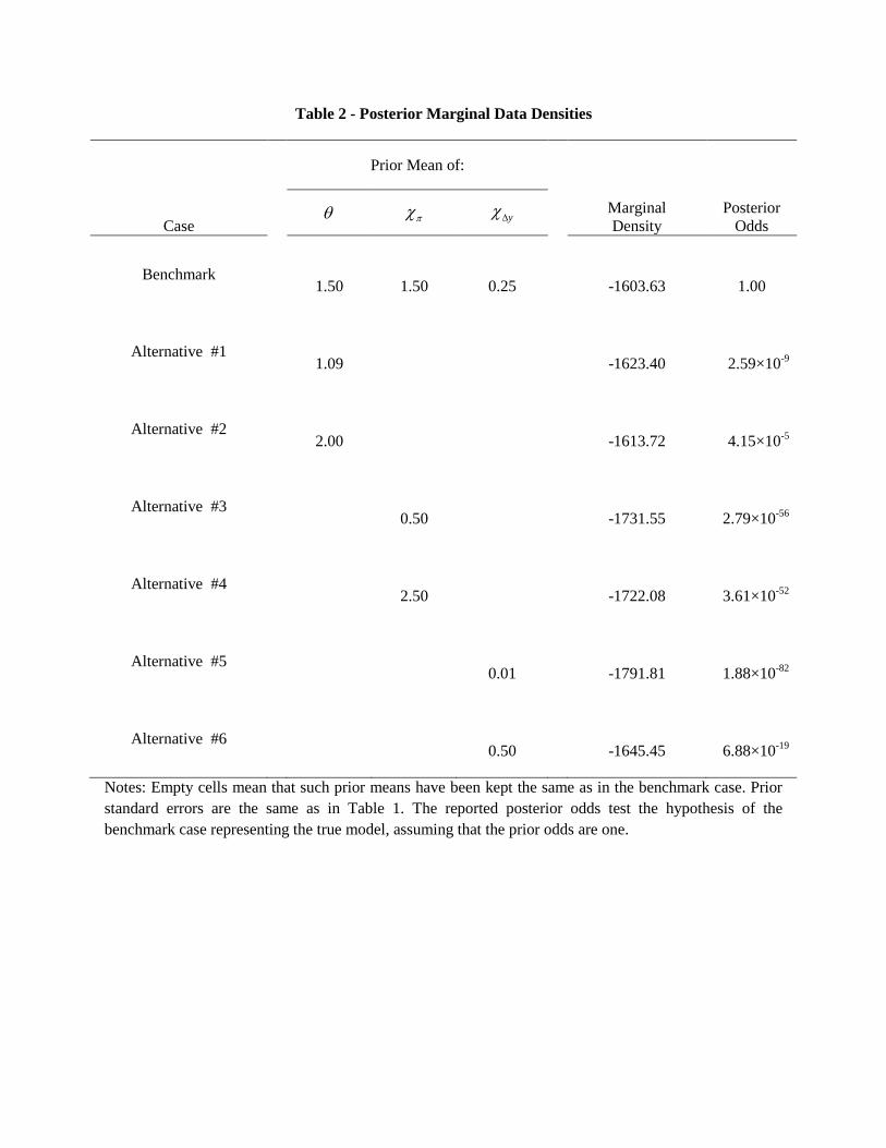
Table 2 - Posterior Marginal Data Densities

Prior Mean of:

Case y

Marginal

Density

Posterior

Odds

Benchmark

1.50 1.50 0.25

-1603.63 1.00

Alternative #1

1.09

-1623.40 2.59×10-9

Alternative #2

2.00

-1613.72 4.15×10-5

Alternative #3

0.50

-1731.55 2.79×10-56

Alternative #4

2.50

-1722.08 3.61×10-52

Alternative #5

0.01

-1791.81 1.88×10-82

Alternative #6

0.50

-1645.45 6.88×10-19

Notes: Empty cells mean that such prior means have been kept the same as in the benchmark case. Prior

standard errors are the same as in Table 1. The reported posterior odds test the hypothesis of the

benchmark case representing the true model, assuming that the prior odds are one.

Table 3 - Forecast Error Variance Decomposition

Variance of:

Accounted for by: Horizon

Output CPI

Inflation

Real

Transport

Costs

Real

Gasoline

Prices

Interest

Rates

Production

Technology

Shocks

4

12

20

∞

32.06

46.57

48.72

49.86

2.80

2.81

2.85

2.89

9.64

11.70

12.34

12.90

8.62

8.64

8.77

8.88

1.92

2.18

2.51

2.80

Gasoline

Endowment

Shocks

4

12

20

∞

41.58

20.04

15.51

13.00

20.23

20.34

20.32

20.30

27.93

28.04

26.64

24.66

41.78

42.00

41.89

41.79

16.64

17.41

17.38

17.33

Transportation

Technology

Shocks

4

12

20

∞

18.85

8.34

6.41

5.36

21.15

20.95

20.92

20.90

7.47

2.76

2.14

1.83

44.12

43.69

43.58

43.48

60.68

58.77

58.49

58.27

Monetary

Policy

Shocks

4

12

20

∞

7.30

24.86

29.19

31.64

55.79

55.89

55.89

55.88

44.29

51.92

54.44

56.81

5.41

5.60

5.69

5.78

20.75

21.63

21.61

21.58

Markup

Shocks

4

12

20

∞

0.21

0.19

0.16

0.13

0.02

0.02

0.02

0.02

10.67

5.58

4.44

3.81

0.06

0.07

0.07

0.07

0.01

0.02

0.02

0.02

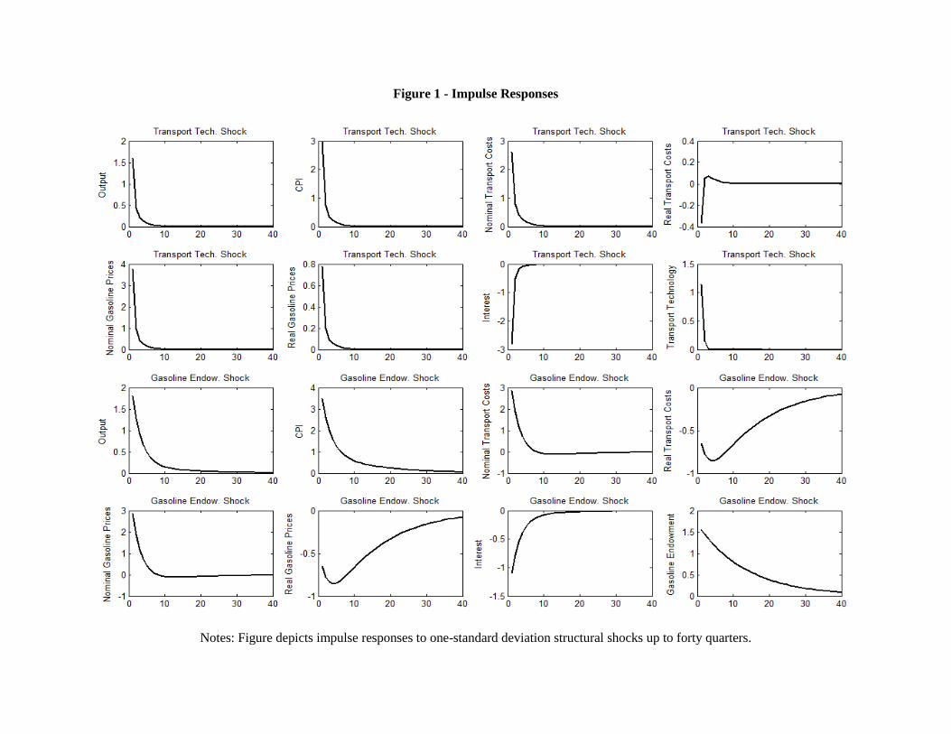
Figure 1 - Impulse Responses

Notes: Figure depicts impulse responses to one-standard deviation structural shocks up to forty quarters.