Gasoline Prices, Government Support, and the Demand

for Hybrid Vehicles in the U.S.

Arie Beresteanu and Shanjun Li∗

JEL Classifications: L62 Q4 Q5

Abstract

We analyze the determinants of hybrid vehicle demand, focusing on gasoline prices

and income tax incentives. We find that hybrid vehicle sales in 2006 would have been

37 percent lower had gasoline prices stayed at the 1999 levels while the effect of the

federal income tax credit program is estimated at 20 percent in 2006. Under the

program, the cost of reducing gasoline consumption was $75 per barrel in govern-

ment revenue and that of CO2 emission reduction was $177 per ton. We show that

the cost-effectiveness of federal tax programs can be improved by a flat rebate scheme.

∗We thank Paul Ellickson, David Genesove, Stephen Holland, Han Hong, Saul Lach, Ian Lange, Wei Tan,Chris Timmins, and two anonymous referees for their helpful comments. Financial support from Micro-Incentives Research Center at Duke University is gratefully acknowledged. Affiliations: Arie Beresteanu,Assistant Professor, Department of Economics, Duke University, Durham, NC 27708-0097, (919)660-1856,arie@econ.duke.edu; Shanjun Li, Fellow, Resources for the Future, 1616 P St. NW, Washington DC 20036,(202)328-5190, li@rff.org.

1 Introduction

Since their introduction into the U.S. market in 2000, hybrid vehicles have been in increas-

ingly strong demand: sales grew from less than 10,000 cars in 2000 to about 346,000 in

2007. A hybrid vehicle combines the benefits of gasoline engines and electric motors and

delivers better fuel economy than its non-hybrid equivalent. Therefore, the hybrid technol-

ogy has been considered as a promising tool in the U.S. to reduce CO2 emissions and air

pollution and to achieve energy security. Following the recommendation of the National

Energy Policy Report (2001),1 the U.S. government has been supporting consumer purchase

of hybrid vehicles in the forms of federal income tax deductions before 2006 and federal

income tax credits since then. The rational for an active governmental role to promote

the diffusion of the hybrid technology is grounded on environmental externalities of motor

gasoline consumption, national energy interests, as well as information spillovers among

consumers and firms often present in the diffusion process of new technologies (Stoneman

and Diederen 1994; Jaffe and Stavins 1999).

In recent years, there have been heightened concerns over adverse environmental ef-

fects of motor gasoline consumption and increasing U.S. dependency on foreign oil.2 To

address energy security and environmental problems, different policies have been proposed

such as increasing the federal gasoline tax, tightening Corporate Average Fuel Economy

(CAFE) Standards, and promoting the development and adoption of fuel-efficient technolo-

gies through subsidies such as tax incentives on hybrid vehicle purchases. Many studies

have examined the first two alternatives, with the majority of them finding that increasing

the gasoline tax is more cost-effective than tightening CAFE standards (e.g., National Re-

search Council 2002; Congressional Budget Office 2003; Austin and Dinan 2005; and Bento,

1The report was written by the National Energy Policy Development Group established in 2001 byGeorge W. Bush. The goal of the group is to develop a national energy policy designed to promotedependable, affordable, and environmentally sound production and distribution of energy for the future.

2The United States imports about 60 percent of its total petroleum products. Motor gasoline con-sumption accounts for an estimated 60 to 70 percent of total urban air pollution and 20 percent of theannual emissions of carbon dioxide, the predominant greenhouse gas that contributes to global warming.See Parry, Harrington, and Walls (2007) for a comprehensive review of externalities associated with vehicleusage and gasoline consumption as well as discussions on policy instruments.

1

Goulder, Jacobsen, and von Haefen 2008). Nevertheless, tightening CAFE standards has

been more politically favorable than increasing gasoline taxes.

Although several studies have looked at consumer adoption of hybrid technology, none

of them investigates the effectiveness of government support on solving energy dependence

and environmental problems through the diffusion of hybrid vehicles (see references below).

In this paper, we analyze the determinants of hybrid vehicle purchase, paying particular

attention to recent rising gasoline prices and government support programs. We investigate

both the overall contribution and the cost-effectiveness of the government programs in

reducing gasoline consumption and CO2 emissions. We then examine the impact of the

program’s regressive nature on its cost-effectiveness by comparing it with a flat rebate

program where all the buyers of the same hybrid model receive an equal subsidy. We

discuss important implications of our findings for the future of the hybrid vehicle market

in the U.S. as well as how to harness the potential benefit of this market for environmental

protection and energy conservation.

Taking advantage of a rich data set of new vehicle registrations in 22 Metropolitan

Statistical Areas (MSA) from 1999 to 2006, we estimate a market equilibrium model with

both demand and supply sides in the spirit of Berry, Levinsohn, and Pakes (1995) (hence-

forth BLP). The demand side is derived from a random coefficient utility model and the

supply side assumes that multiproduct firms engage in price competition. Following Petrin

(2002), our estimation employs both aggregate market-level sales data and household-level

data. The household-level data provide correlations between household demographics and

household vehicle choices, based on which we construct additional moment conditions to

estimate the model. Not only can these micro-moment conditions greatly facilitate the

estimation of consumer preference heterogeneity as illustrated by Petrin (2002), but they

also provide essential conditions for the identification of our empirical model as discussed

in more detail in Section 3.2.

In addition, our estimation method does not rely on the maintained exogeneity assump-

tion in the literature that observed product attributes are uncorrelated with unobserved

product attributes. Because we observe sales of the same product in multiple markets,

2

we use product fixed effects to control for price endogeneity due to market-level unob-

served product attributes following Nevo (2001). Goolsbee and Petrin (2004) employs

an alternative framework where they control for market-specific unobserved product at-

tributes/valuations and identify consumer preference heterogeneity without resorting to

the exogeneity assumption of observed product attributes.

Three recent papers have examined several issues related to hybrid vehicles. Kahn

(2007) studies the effect of environmental preference on the demand for green products and

finds a positive correlation between the adoption of hybrid vehicles and the percentage of

registered green party voters in California. Sallee (2008) studies the incidence of tax credits

for Toyota Prius and shows that consumers capture the significant majority of the benefit

from tax subsidies. A more closely related study to ours, Gallagher and Muehlegger (2007)

estimate the effect of state and local incentives, rising gasoline prices, and environmental

ideology on hybrid vehicle sales and find all three to be important. A major difference

between our study and these papers is that all of them focus on the demand of a single

hybrid model or hybrid vehicles alone while we take a structural method to estimate an

equilibrium model of U.S. automobile market. Our empirical model allows us to simulate

what would happen to the whole market of new automobiles under different scenarios (e.g.,

a different federal support scheme) and to examine the response in the demand and supply

sides separately.

The remainder of this paper is organized as follows. Section 2 describes the background

of the study and data used. Section 3 lays out the empirical model and the estimation

strategy. Section 4 provides the estimation results. Section 5 conducts simulations and

section 6 concludes.

2 Industry Background and Data

In this section, we start by describing the hybrid technology, the U.S. market of hybrid

vehicles, and government support programs. We then discuss the three data sets used in

this study.

3

2.1 Background

The level of fuel economy and emissions produced by a typical automobile is largely a

reflection of low efficiency of conventional internal combustion engines: only about 15

percent of the energy from the fuel consumed by these engines gets used for propulsion,

and the rest is lost to engine and driveline inefficiencies and idling. Hybrid vehicles combine

power from both a gasoline engine and a electric motor that runs off the electricity from a

rechargeable battery. The battery harnesses some of the energy that would be wasted in

operations in a typical automobile (such as energy from braking) and then provides power

whenever the gasoline engine proves to be inefficient and hence is turned off.3

Toyota introduced the first hybrid car, Toyota Prius, in Japan in 1997. In 2000, Toyota

and Honda introduced their hybrid vehicles, Toyota Prius and Honda Insight, into the U.S.

market. With rising gasoline prices, hybrid vehicles have enjoyed an increasing popularity

in recent years. In 2004, as the first U.S. manufacturer into the hybrid market, Ford

introduced its first hybrid model. In 2007, GM and Nissan entered the competition by

introducing their own hybrid models. Table 1 shows the number of hybrid models and

the sales history from 2000 to 2007. The number of hybrid models increased from 2 to

15 during this period.4 The most popular hybrid model, Toyota Prius, accounted for 59

percent of the total new hybrid sales in 2000 and 52 percent in 2007.

Because of the improved fuel economy and reduced emissions, the hybrid technology

is considered as a promising technology by the National Energy Policy Report (2001),

which concludes that the demand for hybrid vehicles must be increased in order to achieve

economies of scale so as to bring the cost of hybrid vehicles down. The group recommended

in the report that efficiency-based income tax incentives be available for the purchase of

new hybrid vehicles. These tax incentives can help offset the higher cost of hybrid vehicles

3Another technology, the fuel cell technology represents a more radical departure from vehicles withinternal combustion engines. They are propelled by electricity created by fuel cells onboard througha chemical process using hydrogen fuel and oxygen from the air. This emerging technology holds thepotential to dramatically reduce oil consumption and harmful emissions. However, fuel cell vehicles arenot soon expected to be commercially viable.

4According to J.D. Power and Associates, there could be 44 hybrid models in the United States by 2012.

4

compared to their non-hybrid counterparts.5 Following the recommendation, the govern-

ment has provided a “clean fuel” tax deduction of up to $2,000 for new hybrid vehicles

placed in service during 2001 to 2005. The Energy Policy Act of 2005 replaced the income

tax deduction with an income tax credit of up to $3,400 for vehicles purchased after Decem-

ber 31, 2005. The tax credit for each model varies and is based on the improvement in fuel

economy provided by that model relative to the non-hybrid counterpart. The credit begins

to phase out over five subsequent calendar quarters for vehicles once the manufacturer sells

a total of 60,000 eligible hybrid vehicles starting from January 1, 2006.6 In addition, some

state and local governments provide benefits to hybrid buyers such as state income tax

deduction/credit, sale tax exemption, High-Occupancy-Vehicle (HOV) lane privileges and

free parking.

2.2 Data

There are three data sets used in this study. The first source is the annual issues of

Automotive News Market Data Book, containing characteristics and number of sales of

virtually all new vehicle models sold in the U.S. from 1999 to 2006.7 Table 2 reports

summary statistics for the 1916 models in this data set. Price is the manufacturer sug-

gested retail prices (MSRP). Size measures the “footprint” of a vehicle. Miles per gal-

lon (MPG) is the weighted harmonic mean of city MPG and highway MPG based on

the formula provided by the EPA to measure the fuel economy of the vehicle: MPG =

5A 2005 report by Edmunds.com finds that a hybrid model can cost about $4,000 more on average thanits equivalent non-hybrid model in terms of purchase price plus ownership costs over the first five years.For example, a Toyota Prius costs $5,283 more than a Toyota Corolla. However, with the average MPGincreases from 35 to 55 MPG, the saving in fuel cost is only about $2,340 over the first five years, assumingannual travel of 15,000 miles and gasoline being $3.00 per gallon.

6It is very likely that another program will be in place after the phase-out of the current program.Several bills regarding tax credits for hybrids have been introduced in the Congress in recent years. Thephase-out works as follows: in the second and third calendar quarter after the calendar quarter in whichthe manufacturer reaches the 60,000 mark, tax credits for hybrid models by this manufacturer become 50percent of their original amounts. They are then reduced to 25 percent in the fourth and fifth calendarquarter and to zero thereafter. Toyota reached the 60,000 mark in June 2006. From October 1, 2006 tothe end of March, 2007, hybrid vehicles by Toyota are only eligible for 50 percent of original tax credits.

7Exotic models with tiny market shares such as Farrari are excluded.

5

1/(0.55/city MPG + 0.45/highway MPG). The vehicles are divided into 4 categories (car,

van, SUV, and pickup truck) and further classified into 15 segments based on vehicle at-

tributes and market orientations.

The second data set contains vehicles sales data in 22 selected MSAs from 1999 to

2006. Accounting for about 15.3 percent of total U.S. vehicles sales, these MSAs are

chosen from all 9 census divisions and have large variations in terms of size and average

household demographics. This vehicle sales data set, purchased from R.L. Polk Company,

contains total annual sales for each of the 1619 models in all 22 MSAs with the exception

of Albuquerque, NM and Little Rock, AR, where we have sales data only from 2001 to

2006. In total, we have 34,860 observations of sales data for the 22 MSAs. These MSAs are

well representative of the national data in terms of average household demographics and

vehicle fleet characteristics.8 Table 3 presents the total number of new vehicle sales, the

percentage of hybrid vehicles, availability of local and state incentives, and gasoline prices

in 2006. The percentage of hybrid vehicles in total new vehicle sales is highest in San

Francisco and lowest in Miami among the 22 MSAs. The average market share of hybrid

vehicles is 2.86 percent in the MSAs with local incentives while being 1.75 percent in the

MSAs without local incentives. The last column of Table 3 gives annual average gasoline

prices in each of the MSAs. They are the average of quarterly prices collected from the

American Chamber of Commerce Research Association (ACCRA) data base. There are

large variations in gasoline prices in both cross-sectional and temporal dimensions in the

data.

Our first data set describes vehicle choices consumers face while the second data set

presents consumer purchase decisions at the aggregate level in the 22 MSAs. The third

data set, the 2001 National Household Travel Survey (2001 NHTS), helps link household

demographics with purchase decisions. The survey, often used to study national trans-

portation trends, was conducted by agencies of the Department of Transportation from

March 2001 through May 2002 through random sampling. This data set provides detailed

8The correlation coefficient between model sales in the 22 MSAs and the national total is 0.94. Moredetails on the representativeness of these MSAs are given in Li, Timmins and von Haefen (2009) .

6

household level data on vehicle stocks, travel behavior, and household demographics at the

time of survey. There are 69,817 households and 139,382 vehicles in the data. Among all

the surveyed households, 45,984 are from MSAs.

Column 1 in Table 4 shows the means of several demographics for households living in

MSAs. Renter, a dummy variable, is equal to 1 for the households that living in rented

houses and 0, otherwise. Children dummy is 1 for households with children. Columns 2

to 6 present the means of household demographics for different groups based on household

vehicle choice. These conditional means provide additional moment conditions in our esti-

mation where we match the predicted moments from the empirical model to these observed

moments. As household incomes are categorized and top-coded at $100,000, we provide

the probability of new vehicle purchase for six income groups in the second panel of Table

4. In our estimation of the empirical model, these conditional probabilities are matched by

their empirical counterparts based on model predictions for 2001 and 2002.

3 Empirical Model and Estimation

In this section, we discuss our empirical model and estimation strategy, which follows recent

empirical literature on differentiated products. The empirical model includes both demand

and supply sides. Vehicle demand is derived from a random coefficient discrete choice

model while the supply side assumes that multiproduct firms, taking product choices as

given, engage in price competition.

3.1 Empirical Model

Let (Ω, A , P) be a probability space where Ω is the set of households, A is the Borel set

of Ω, and P is a distribution function. Let i ∈ A denote a household and j ∈ J denote

a product where J is the choice set. Household i’s utility from product j is a function

of household demographics and product characteristics. A household chooses one product

from a total of J models of new vehicles and an outside alternative in a given year. The

7

outside alternative captures the decision of not purchasing any new vehicle in the current

year. To save notation, we suppress the market index m and time index t, bearing in mind

that the choice set can vary across markets and years. The utility of household i from

product j (in market m at year t) is defined as

(1) uij = u(pij, Xj, ξj, yi, Zi) + εij,

where pij is the price of product j for household i. The price is computed based on

the MSRP, the sales tax and federal income tax incentives for hybrid vehicles.9 Xj is a

vector of observed product attributes, ξj the unobserved product attribute, yi the income

of household i, and Zi is a vector of household demographics. εij is a random taste shock.

The specification of the first term in the utility function is assumed to be:

(2) uij = αipij +K∑

k=1

xjkβik + ξj.

αi measures consumer i’s preference for price changes. We model αi to be inversely pro-

portional to the income of the household αi = α/yi.10 xjk is the kth product attribute

for product j. βik is the random taste parameter of household i over product attribute k,

which is a function of household demographics including those observed by econometrician

(zir) and those that are unobserved (νik):

(3) βik = βk +R∑

r=1

zirβkr + νikβuk .

Although the utility specification we use is standard in the literature, it misses several

9MSRPs, also known as “sticker prices”, are set by manufacturers and are generally constant acrosslocations and within a model year. Although individual transaction prices are desirable in the analysisof automobile demand given that different consumers may pay different prices for the same model, thesedata are not easily available. MSRPs have been commonly used in this literature. The implications arediscussed extensively below.

10This functional form for the interaction between income and price, also used in Berry, Levinsohn,and Pakes (1999), can be derived as a first-order Taylor series approximation to the Cobb-Douglas utilityfunction originally used in BLP.

8

potentially important features of automobile demand. First, automobiles are durable goods

and transaction costs exist in the second-hand market. Therefore, consumer expectations

about future prices, as well as future gasoline price may be important factors to consider.

Second, current household demand for automobiles may be affected by current vehicle

holdings or past experiences. Third, the interaction between the market of new vehicles

and that for used vehicles may be important as well. Incorporating these factors into the

demand estimation is challenging and is left for future research. A notable recent attempt

to address these issues is Bento et al. (2009) where they model both new vehicle demand

and used vehicle holdings simultaneously.

Based on the utility function, we can derive the aggregate demand function. Define θ as

the vector of all preference parameters in equations (2) and (3), and the set of individuals

who choose alternative j is

(4) Aj =

i : uij = maxh∈0,1,...,J

uih

,

where uih is defined by (1). Product 0 is defined as the outside alternative and the utility

from it is normalized to be zero in the estimation. The aggregate demand for model j is

given by

(5) qj = P(Aj),

where P is the population distribution function. We assume that the random taste shock

ε has a type I extreme value distribution and that unobserved household demographics ν ′s

are from normal distributions with zero mean and standard deviations to be estimated.

The distribution of observed household demographics Z is based on U.S. census data.

The demand side parameters can be estimated without a supply side model. However, a

supply side model is needed for the counterfactual analysis where we solve for the prices in

a new equilibrium based on firms’ price-setting rules derived from the profit maximization

problem. Following the literature, we assume that firms engage in Bertrand competition

to maximize the period profit from the whole U.S. market while taking the product mix

9

as given. To understand the effect of this assumption on our results, we also perform

robustness analysis where we only rely on the demand side model, i.e., prices are assumed

be fixed in Section 5.5.

The period total variable profit (total revenue minus total variable cost) of a multiprod-

uct firm f is

(6) πf =∑

j∈F(f)

[pjqj(p, θ)− vcj(qj)

],

where F(f) is the set of products produced by firm f . pj is the price and qj is the sales for

product j. vcj is the total variable cost of product j.11 The first order condition of firm f

with respect to pj is:

(7)∑h∈F

[ph −mch(qj)

]∂qh(p, θ)

∂pj

+ qj(p, θ) = 0.

The equilibrium price vector is defined, in matrix notation, as

(8) p = mc(q) + ∆−1q(p, θ),

where the elements of ∆ are

∆jr =

−∂qr

∂pjif product j and r produced by same firm

0 otherwise.(9)

Equation (8) underlies the pricing rule in a multiproduct oligopoly: equilibrium prices

are equal to marginal costs plus markups, ∆−1q(p, θ). The implied marginal costs can be

computed following mc = p−∆−1q, where p and q are the observed prices and sales. In a

11We do not consider the role of the CAFE constraints on firms’ pricing decision here. See Jacobsen(2007) for an examination of how firms, particularly U.S. firms underprice their fuel-efficient vehicles inorder to meet the CAFE standards. In recent years, the CAFE constraints have not been binding forToyota and Honda who produces the majority of the hybrid vehicles.

10

counterfactual analysis, the fixed point of equation (8) can be used to compute new price

equilibrium corresponding to a change in the demand equation q(p, θ), providing that we

know the relationship between mc and q. Constant marginal cost assumption has been

commonly used in recent literature on estimating automobile market equilibrium (e.g.,

Bresnahan 1987; Goldberg 1995).12 If marginal costs are not constant with respect to the

total output level, the functional relationship between the two has to be recovered in order

to find new equilibrium prices in counterfactual scenarios.

3.2 Estimation

The preference parameters in the utility function are estimated by matching the predicted

sales as shown in equation (5) with observed sales in each market. The predicted sales

are computed based on a random sample of households from the 2000 Census data while

taking into account various government support programs for hybrid vehicles. Because the

federal incentives for hybrid vehicles are in the forms of income tax deductions or income tax

credits, they may vary across households depending on household tax liabilities: households

with fewer tax liabilities tend to enjoy less tax benefit from buying a hybrid vehicle. To

figure out tax incentives for each household, we calculate household income tax liabilities

using NBER’s online software TAXSIM (version 8.0). TAXSIM takes household income

sources and other demographics from survey data as input and returns tax calculations as

output.13

To illustrate our estimation strategy, which exploits the fact that we observe the demand

for each product in many MSAs, we bring the market index m into the utility function and

write the utility function as

umij = δmj + µmij + εmij,(10)

12The constant marginal cost assumption does not rule out the existence of economies of scale. A highfixed cost and constant marginal cost can still result in economies of scale.

13TAXSIM and an introduction by Feenberg and Coutts (1993) are available athttp://www.nber.org/taxsim.

11

where δmj, the mean utility of product j in market m, is the same for all the households

in market m. It can be further specified as follows

δmj = δj + Xmjγ + emj,(11)

where δj is a product dummy, absorbing the utility that is constant for all households

across the markets (including the utility derived from the unobserved product attributes

ξj). Xmj is a vector of product attributes that vary across MSAs. It includes dollars per

mile (DPM), which is the gasoline price in market m divided by the MPG of product j.

DPM captures the fuel cost per mile for a vehicle. emj is the part of the mean utility that

is unobserved to researchers. µmij is the household specific utility. Following notations in

equations (2) and (3), the household specific utility is:

µmij = αpij

yi

+∑kr

xmjkzirβkr +∑

k

xmjkνikβuk .(12)

Denote the parameters in the mean utility as θ1 = δj, γ, and the parameters in the

household specific utility as θ2 = α, βkr, βuk.

Because we do not have data on vehicle retail prices at the MSA level and instead use

MSRPs, variations in retail prices across markets enter the error term, emj, in equation (11).

Moreover, emj also captures marketing efforts at the local level such as advertisement. These

unobserved factors may render explanatory variables in Xmj in equation (11) endogeneous.

For example, retailers in areas/years with high gasoline prices may offer deeper discounts

for fuel-inefficient vehicles than those in areas/years with low gasoline prices. Without

controlling for unobserved factors, consumer response to gasoline prices may be under-

estimated.14

Taking advantage of the multiple-market feature of our data set, we use the fuel cost

per mile in MSAs that are not geographically close to a given MSA as instruments for

14The correlation between marketing efforts and vehicle fuel cost per mile can also arise at the nationallevel. However, unobserved national promotions can be treated as an unobserved product attribute andtherefore subsumed in product fixed effects δj .

12

endogenous variables in that MSA. Specifically, for a vehicle model in MSA m, we use the

average fuel cost per mile of the same model in all the MSAs in a different census region (4

census regions in total) and that in a different division (9 divisions in total), giving rise to

two excluded instruments. Similar ideas for instruments have been explored in Hausman

(1996) and Nevo (2001) where data on multiple markets are available. The validity of

these instruments hinges on the assumption that local promotions are not correlated across

distant MSAs.

BLP shows that given a vector of θ2, a contraction mapping technique can be used to

recover the unique vector of δmj for each market that equalizes predicted market shares with

observed market shares. With the recovered δmj, θ1 can be estimated using the instrumental

variable method in a linear framework following equation (11). The estimation strategy

is a simulated GMM with the nested contraction mapping discussed above. We construct

two sets of moment conditions, with the first set being based on equation (11):

E[emj(θ1, θ2)|Lmj

]= 0,

where L includes the two constructed instruments and variables in X that are assumed to

be exogenous to the error term.

The second set includes 22 micro-moments which match the model predictions to the

observed conditional means from the 2001 NHTS as shown in Table 4. For example, we

match the predicted probability of new vehicle purchase among households with income

less than $15,000 to the observed probability in the data.

P(i ∈

J⋃j=1

Aj|yi < 15, 000; δm(θ2), θ2

)= 0.002,

where Aj is defined in equation (4). Petrin (2002) demonstrates that adding micro-moments

based on household-level data can dramatically improve the estimation of preference pa-

rameters that capture consumer heterogeneity. We extend his approach of taking advantage

of micro data to facilitate estimation in that we do not rely on the maintained exogene-

13

ity assumption in the literature that unobserved product attributes are uncorrelated with

observed product attributes for model identification.

Instead, we take advantage of the multi-market feature of our data by using prod-

uct fixed effects to deal with price endogeneity due to unobserved product attributes. This

strategy of controlling for unobserved product attributes has been employed by Nevo (2000)

and Nevo (2001) where sales of the same products are observed in multiple markets. A

practical difference between his approach and ours is that because our first set of mo-

ment conditions is not enough to identify θ2, the micro-moment conditions are therefore

essential for the identification of our model. Goolsbee and Petrin (2004) provide an alter-

native empirical strategy in a multinomial probit framework that allows for market-specific

unobserved attributes/valuations for the same product across markets. By employing a

simulated maximum likelihood method based on household-level data, the identification

of consumer heterogenous preference parameters in their model also does not rely on the

exogeneity assumption of observed product attributes.

We form the objective function by stacking the two sets of moment conditions. The

GMM estimators θ1 and θ2 minimizes: J = M(θ1, θ2)′WM(θ1, θ2), where M(θ1, θ2) includes

the two sets of moment conditions and W is the weighting matrix. The procedure involves

iteratively updating θ2 and then δmj to minimize the objective function. The estimation

starts with an initial weighted matrix to obtain consistent initial estimates of the parameters

and optimal weighting matrix. The model is re-estimated using the new weighting matrix.

With the estimation of the demand side, we can recover the marginal cost for each

model based on firms’ first order condition for profit maximization in equation (8). The first

order condition can also be used to simulate new equilibrium prices in the counterfactual

scenarios. To check if marginal costs are constant with respect to the output level, we

estimate the following equation based on implied marginal costs:

(13) mcj = ωjρ + ζj,

where ωj includes model attributes and U.S. sales. Because U.S. domestic sales of a model

14

often do not coincide with total production of the model due to international trade and data

on model-level production are not readily available, we use vehicle sales as the proxy for

production. ζj is the error term which may include production cost from unobserved prod-

uct attributes as well as productivity shocks. An endogeneity problem arises in estimating

the non-constant marginal cost function given that sales are related to unobserved product

attributes. Only in this context, we invoke the maintained identification assumption in the

differentiated product literature that unobserved product attributes are mean independent

of observed product attributes. Based on this assumption, instruments for vehicle sales are

provided by the observed attributes of competing products.15

4 Estimation Results

We first report parameter estimates for the random coefficient model and then use these

estimates to calculate price elasticities and implied price-cost margins. After that, we

present estimation results from alternative estimation strategies.

4.1 Parameter Estimates

Table 5 provides two sets of estimation results. In columns 2 and 3, the fuel cost variable,

DPM, is assumed to be exogenous while in columns 4 and 5 the possible endogeneity

of DPM is controlled for. We use two instruments as discussed in the previous section:

the average DPM of the same vehicle in MSAs of different census divisions, and that in

MSAs of different regions. In both cases, the coefficient on DPM is negative and estimated

precisely, implying that a vehicle with better fuel efficiency hence smaller DPM is valued

more than a less fuel-efficient vehicle, ceteris paribus. The identification of this coefficient is

based on the cross-MSA sales variations in response to differences in gasoline prices across

MSAs: a fuel-efficient vehicle should be more popular in a high gasoline price area than

otherwise, all else equal. The coefficient estimate on DPM is larger when DPM is assumed

15Our estimation results, available from the authors, cannot reject the constant marginal cost assumption.

15

to be endogenous and instrument variables are applied than when DPM is assumed to be

exogenous. This finding confirms the presence of local unobservables such as promotions

that are positively correlated with vehicle fuel cost.

Local support dummy is equal to 1 for hybrid models in MSAs where local government

supports such as HOV lane privilege and free meter parking are available for hybrid vehicles.

The interaction terms between MSA dummies and the hybrid dummy capture unobserved

heterogeneity on hybrid demands that may arise from differences in dealer availability and

consumer attitudes toward hybrid vehicles. We include interaction terms between MSA

dummies and vehicle type dummies (i.e., car, SUV, van, and pickup truck) to control for

unobserved heterogeneity in consumer preference for each type of vehicles across MSAs.

For example, consumers in MSAs with more snow and slippery driving conditions might

prefer SUVs and pickup trucks, which are often equipped with a four-wheel-drive.

Table 5 also presents the estimates of the parameters in the household specific util-

ity defined by equation (12). These parameters capture consumer heterogeneity due to

observed and unobserved household demographics. The first three coefficients capture het-

erogeneity in consumer preference on vehicle price. The coefficient for high income groups

being larger implies richer households are less price sensitive. The second four parameters

are for the interaction terms between vehicle size and four demographic variables. These

interaction terms allow families with different households to have different tastes for ve-

hicle size. These coefficient estimates suggest that households living in their own houses

and those with children prefer larger vehicles. Table 5 then reports the estimates of seven

random coefficients, which measure the dispersion of heterogeneous consumer preference.

These coefficients are the standard deviations of consumer preferences for the correspond-

ing product attributes. For example, the preference parameter on DPM has a standard

normal distribution with mean -8.618 and standard deviation 5.768. The estimates suggest

that over 93 percent of the households have a negative preference parameter on DPM.

The random coefficients ultimately break the independence of irrelevant alternatives (IIA)

property of standard logit models in that the introduction of a new vehicle model into

the choice set will draw disproportionately more consumers to the new model from similar

16

products than from others.

4.2 Elasticities and Price-cost Margins

Based on the parameter estimates for the demand side, we compute own- and cross-price

elasticities. A sample of these elasticities are reported in Table 6. One obvious pattern

from this table is that the demand for cheaper products tends to be more price sensitive.

Moreover, cross-price elasticities are larger among similar products, suggesting that substi-

tutions occur more often across similar products than dissimilar ones when prices change.

For example, the cross-price elasticities for Toyota Corolla suggest that when its prices

increase, consumers are most likely to switch to Toyota Camry and Toyota Prius (Corolla’s

hybrid counterpart) among the 10 competing models in the table.

We recover the marginal cost for each product from firms’ first order conditions based

on the demand side estimates and the Bertrand competition assumption in the supply side.

We then can compute price-cost margins aspj−mcj

pj, some of which are reported in the last

column of Table 6. Among the 8 non-hybrid models, Cadillac Escalade, the most expensive

product, has the largest margin of 33.67 percent. Interestingly, although Toyota Prius is

cheaper than Toyota Camry hybrid, it has a smaller price sensitivity and a higher margin.16

Overall, there appears to be a large variation in the estimates of both elasticities and price-

cost margins. Among the 1,619 products, the sales weighted average own-price elasticity

is -8.40 while the weighted average price-cost margin is 17.72 percent. Our estimate of

average margins is closest to Petrin (2002)’s estimate of 16.7 percent which is based on 185

vehicle models per year sold from 1981 to 1993 including cars, vans and pickup trucks. The

average benchmark margin in BLP is estimated at 23.9 percent for cars sold between 1971

and 1990 while Goldberg (1995) recovers a much larger estimate of 38 percent for cars from

1983 to 1987, both of which are based on about 110 models per year.

Since the preference parameter on the fuel cost of driving, DPM, is one of the key

16To the extent that some consumers advertise themselves as environmentalists by driving hybrid vehicles(Kahn (2007)), Prius’s distinct appearance makes the model less substitutable than other hybrid modelssuch as Toyota Camry hybrid which has the same look as the non-hybrid Camry.

17

parameters of interest, it is helpful to verify whether the parameter estimate is in line

with simple calculations based on fuel costs of driving and price elasticities. Take a Toyota

Camry as an example. Its average fuel cost of driving in the 22 MSAs is 9.47 cents per mile.

Our demand model predicts that a 1.5 cent increase in the fuel cost of driving for Toyota

Camry alone would result in a 9.74 percent decrease in its sales, holding vehicle prices

fixed. To compare the model prediction with a back-of-the-envelop calculation, assume

vehicle miles traveled to be 12,000 per year, vehicle lifetime to be 15 years, and a discount

factor of 0.98. The increase in total discounted fuel cost during vehicle lifetime is therefore

about $235, 1.18 percent of the price of the vehicle. Our estimated price elasticity being 9

implies that an increase of 1.18 percent in vehicle price would cause about 10.62 percent

in reduction in quantity demanded. We take comfort in the fact that our model prediction

of 9.74 percent decrease is close to that from the above intuitive calculation.

4.3 Alternative Specifications

The results discussed above are based on the empirical model where product fixed effects

are used to control for unobserved product attributes and national level promotions, both

of which can be correlated with observed product attributes. To examine the importance

of this strategy, we estimate the model without including product fixed effects and instead

employ the maintained exogeneity assumption in the literature that observed product at-

tributes are uncorrelated with the unobserved product attributes. In the estimation, we

add vehicle size, horsepower as well as 15 vehicle class dummies, which would be otherwise

subsumed in product dummies.

Table 7 presents two sets of estimation results without using product dummies. One set

is based on the assumption that DPM is exogenous while the other is from the model where

the endogeneity of DPM due to local promotions is dealt with using DPM in other MSAs as

instruments. In both cases, we control for the endogeneity of the vehicle price variable with

two instruments constructed based on observed product attributes.17 It is worth noting

17We construct two “distance” measures for each product. The distance measures reflect how differen-tiated a product is from other products within the firm and outside the firm. The measures are based on

18

that the presence of national level promotions that are correlated with product attributes

such as vehicle fuel efficiency would render both sets of instruments invalid.

The model where the endogeneity of DPM is controlled for suggests a larger consumer

response to the fuel cost per mile. The parameter estimates from this model imply that the

sales-weighted average own-price elasticity and price-cost margin are respectively, -9.06 and

18.26 percent, similar to -8.40 and 17.72 percent from our preferred model in the previous

section. However, the results suggest that consumers are about twice as sensitive to the

fuel cost of driving as what is implied by the results in the previous section. This finding

suggests that the exogeneity assumption regarding observed product attributes may be

violated.

5 Simulations

In this section, we conduct simulations to examine the effect of rising gasoline prices and

federal tax incentives on the diffusion of hybrid vehicles. We compare the current income

tax incentive program with a rebate program in terms of their cost-effectiveness and their

effects on industry profits. Our simulations assume that product offerings would stay the

same under different scenarios.18 To the extent that both run-ups of the gasoline price

and federal tax incentives strengthen consumer incentives to purchase hybrid vehicles and

therefore increase firms’ incentive to offer more hybrid models, our static analysis would

under-estimate the true effects of these two factors.

distances between two products in a Euclidean space where different weights are applied to different dimen-sions of the product-characteristics space. The weights are the coefficients of the corresponding productattributes in a hedonic price regression.

18The decision of product choice, although an interesting topic, is out of scope of this paper. A structuralapproach to this topic involves modeling a dynamic game where the model should contend with severalkey facts about the auto industry: the industry consists of several big players that act strategically; eachof them produces multiple products; and products are differentiated.

19

5.1 Gasoline Prices

Understanding how consumers’ vehicle choice decisions respond to changes in gasoline prices

has important implications for policies that aim to address energy security and environmen-

tal problems related to gasoline consumption. We study the effect of changes in gasoline

prices on hybrid vehicle sales by simulating the market outcomes under different gasoline

price scenarios. In preforming the simulations, we solve new equilibrium prices under each

scenario based on the estimates of demand parameters and product marginal costs, as-

suming multiproduct firms engage in price competition. We then estimate sales for the 22

MSAs under new equilibrium prices.

The first simulation investigates what would have happened if gasoline prices from 2001

to 2006 had been the same as those in 1999 in each of the 22 MSAs. Column (2) in Table

8 presents the effects of gasoline price changes on prices of five hybrid models and their

non-hybrid counterparts in 2006. The average gasoline price in the 22 MSAs weighted

by vehicle sales was $1.53 in 1999 and $2.60 in 2006. If gasoline prices had stayed at

the 1999 levels, the five selected hybrid models in 2006 would have been 4 to 10 percent

cheaper because they would have been in weaker demand given that the savings in fuel

cost would be smaller. For their non-hybrid counterparts, the changes in prices are smaller

in magnitude as the differences in fuel cost would be smaller. The prices of Ford Escape

and Toyota Highlander, for example, would have been higher with gasoline prices staying

at the 1999 levels while three more fuel-efficient vehicles would have been slightly cheaper.

Column (4) in Table 8 shows the effect of gasoline price changes on sales. The decrease in

sales in the 22 MSAs for the five hybrid models ranges from 21 to 38 percent have gasoline

prices stayed at the 1999 levels. The effect on more fuel-efficient hybrid models such as

Honda Civic hybrid and Toyota Prius, is more significant. On the other hand, without the

gasoline price increase in 2006, the sales of regular Ford Escape would have increased by

about 25 percent while that of Honda Civic and Toyota Corolla would have dropped by 15

and 6 percent, respectively.

Table 9 presents the effect of rising gasoline prices on total sales of hybrid vehicles in the

20

22 MSAs from 2001 to 2006. Column (1) lists the annual average gasoline price weighted

by vehicles sales. Gasoline prices have been continuously increasing over the years except

in 2002. In the absence of these increases, the sales of hybrid vehicle would have been

significantly less.19 This simulation shows that the gasoline price is indeed an important

factor in hybrid vehicle purchase decisions. The $1.07 increase in the gasoline price in 2006

over that in 1999 explains almost 37 percent of hybrid vehicle sales. To speak to the record

high gasoline price of $4 per gallon observed in mid-2008, we also simulate the effect of

more dramatic increases in gasoline prices on hybrid vehicle sales. Columns 4 and 5 in

Table 9 present the percentage increases in sales if gasoline prices were at $4 and $6 per

gallon in 2006. The results show that if the gasoline price was $4 per gallon in the 22

MSAs, the sales of hybrid vehicles would have been 65 percent higher in 2006.

5.2 Federal Tax Incentives

In this section, we conduct simulations to investigate the effect of federal income tax incen-

tives on hybrid vehicle purchases. We first simulate the would-be market outcomes in the

absence of these incentives during the period. Table 10 presents the effects of the income

tax incentives on both prices and sales of several selected hybrid models in 2005 and 2006.

Column (1) shows the price of each model in 2006 dollars while column (2) gives the total

sales in the 22 MSAs. Column (3) lists the average tax benefit received by buyers of each

model. In 2005, the $2,000 tax deduction yields $371 income tax return for Ford Escape

hybrid buyers on average. In 2006, hybrid buyers are eligible for up to $2,600, $2,100, $650

and $3,150 tax credit for the purchase of a Ford Escape hybrid, Honda Civic hybrid, Honda

Accord hybrid and Toyota Prius, respectively. The tax credit program is more generous for

most hybrid models than the tax reduction program. For example, buyers of Ford Escape

hybrid on average received $1,960 income tax return for their purchase in 2006, comparing

to only $371 in 2005.

19Although the average gasoline price in 2002 was about the same as that in 1999, the sales of hybridvehicles would have been less in our simulation. This is because gasoline prices actually dropped in 2002in several MSAs with strong demand for hybrid vehicles such as San Francisco, San Diego, and Seattle.

21

Without tax incentives, both prices and sales of these hybrid models would be reduced.

The supply price of a 2005 Ford Escape hybrid would be $190 (0.67 percent) lower as shown

in column (4), comparing to the $371 tax benefit received by an average buyer. For Toyota

Prius, the supply price would drop by $197 (0.89 percent) in 2005 in the absence of income

tax deductions, comparing to $522 tax benefit received by Prius buyers on average. These

numbers suggests that buyers capture about 50-60 percent of the government subsidy and

the supplier about 40-50 percent. This finding also holds for other hybrid models based on

average tax benefits received by buyers in column (3) and price decreases in the absence

of government subsidy in column (4).20 The effect of tax incentives on hybrid vehicle sales

in 2005 is less than 4 percent for the five hybrid models shown in the table. However, the

effect of more favorable tax incentives in 2006 is much more significant: for 2006 Toyota

Prius, about 25 percent of its sales can be attributed to the tax credit policy in place.

Table 11 presents the effect of tax incentives on total hybrid sales in the 22 MSAs from

2001 to 2006. Column (2) gives average tax returns received by hybrid buyers in 2006

dollars. They are decreasing from 2001 to 2005 due to two facts. First, while the tax

deduction is kept at a nominal level of $2,000, the inflation is about 14 percent over this

period. Second, the number of households subject to Alternative Minimum Tax (AMT)

increases significantly. These households are not eligible for the full tax benefit when buying

hybrid vehicles. In 2006, federal government support, in the form of income tax credits, is

much stronger: the tax benefit received by each hybrid buyer is $2,276 on average. Based on

column (3), about 20 percent of the total hybrid sales in the 22 MSAs could be explained by

tax credits, comparing to less than 5 percent in previous years. It is interesting to note that

hybrid sales, although smaller, would still be growing dramatically over time even without

tax incentives. Columns(4) and 5 present the average tax benefit received by hybrid vehicle

buyers and the changes in hybrid vehicle sales in percentage if federal income tax incentives

20Our estimates show that buyers of Toyota Prius in 2006 capture about 63 percent of total federaltax incentives. Sallee (2008) estimates that buyers of 2006 Toyota Prius get at least 73 percent of totaltax subsidies using detailed retail price data. In order to explain the finding that consumers capture thesignificant majority of the benefit from federal tax subsidies in the case of Toyota Prius, whose productionwas capacity constrained in 2006, he suggests a model where current vehicle prices influence future demand(e.g., due to goodwill).

22

had been doubled. In 2006, each hybrid vehicle buyer would have received $4,754 in tax

benefit and the sales of hybrid vehicles would have been about 23 percent larger than the

observed sales in 2006.

5.3 Gasoline Consumption and CO2 Emissions

In 2005, U.S. motor gasoline consumption was 9.16 million barrels per day, accounting

for about 45 percent of total U.S. petroleum consumption according to the Department

of Energy. Total CO2 emissions from motor vehicle usage was 3.78 million tons per day,

accounting for about 20 percent of total U.S. CO2 emissions. Therefore, having a more

fuel-efficient vehicle fleet is an important step toward solving energy security and climate

change problems. In the previous two subsections, we have studied the effects of two

important factors, gasoline price run-ups and income tax incentives, on the the diffusion of

hybrid vehicles in recent years. We now turn to the implications of two policy alternatives,

federal gasoline taxes and income tax incentives, on total U.S. gasoline consumption and

CO2 emissions.

Table 12 presents policy impacts on four variables: average MPG of new vehicles sold in

2006, total new vehicles sales in 2006, total gasoline consumption, and total CO2 emissions.

Both total gasoline consumption and CO2 emissions are calculated for the 2006 cohort of

new vehicles during the lifetime of these vehicles. Column (1) shows that the average MPG

of new vehicles in 2006 would have been 23.09 in the absence of federal income tax credits,

compared to observed 23.19, while the doubling of the incentives would have increased the

average MPG from 23.19 to 23.31. To compare the effectiveness of the tax incentives with

that of a higher gasoline tax, we examine an increase in the federal gasoline tax of 10 cents,

25 cents, and 1 dollar.21 The simulation results suggest that an increase of 10 cents in

gasoline taxes would generate the same impact on the average MPG with that produced

21Among industrial countries, the U.S. has the lowest gasoline tax (41 cents per gallon on averageincluding 18 cents of federal tax). Meanwhile, Britain has the highest gasoline tax of about $2.80 pergallon. In simulations, we assume that these gasoline tax increases would generate equivalent increases ingasoline prices. To the extent that the gasoline industry is not perfectly competitive, results from thesesimulations should be viewed as upper bounds of the true effects.

23

by the income tax credit program. The key difference between the two types of policies is

illustrated by column (2), which presents the changes in total sales of new vehicles under

different policies. It shows that the two types of policies have an opposite effect on new

vehicle sales: while the tax credit program increases new vehicle sales (by increasing hybrid

vehicle sales), a higher gasoline tax would achieve the opposite.

Columns (3) and (4) in Table 12 presents total reductions in gasoline consumption and

CO2 emissions in the U.S. over vehicle lifetime for vehicles sold in 2006.22 Due to the

small number of hybrid models available and the small market share of hybrid vehicles,

the reductions in both gasoline consumption and CO2 emissions from the income tax credit

program are inconsequential relative to their total amounts. On the other hand, our results

show that an increase in the gasoline tax of only 10 cents would generate much larger reduc-

tions. A $1 dollar increase in the gasoline tax would reduce gasoline consumption and CO2

emissions by over 16 percent. Our analysis shows that to achieve the 20 percent gasoline

consumption reduction in 10 years as proposed in the 2007 State of the Union Address,

higher gasoline prices (e.g., through a higher gasoline tax) represent a more promising

avenue.

We now examine the cost of reducing gasoline consumption and CO2 emissions in terms

of the foregone tax revenue in income tax incentive programs. Based on our model esti-

mates, the total federal income incentives to hybrid buyers in the 22 MSAs were 134.43

million dollars in 2006 while the reductions in gasoline consumption and CO2 emissions

are 1.80 million barrels and 0.76 million tons, respectively. This implies that the cost of

gasoline consumption reduction through the income tax credit program is $75 per barrel

with a 90 percent confidence interval of [72, 78] while the cost of CO2 emission reduction

is $177 per ton with a 90 percent confidence interval of [170, 184]. By comparison, Metcalf

(2008) finds that, in the context of tax credits for ethanol, using tax revenues to achieve

energy policy is highly cost ineffective. He estimates that the cost of reducing gasoline

consumption through tax credits for ethanol is $85 per barrel in 2006 and the cost of re-

22Assume that vehicle lifetime is 15 years and average annual travel is 12,000 miles per vehicle. Thecombustion of one gallon gasoline generates 19.5 pounds of CO2 according to the Energy InformationAdministration.

24

ducing CO2 emissions is $1,700 per ton.23 Our estimates show that the tax credit program

for hybrid vehicles, although still costly, is more effective than the tax credit program for

ethanol, especially in reducing CO2 emissions from the point view of government revenue.

It is worthwhile to point out two caveats underlying these results. First, we assume

that both vehicle miles traveled and the vehicle lifetime are fixed. Studies have shown

that high gasoline prices tend to reduce vehicle miles traveled (see Small and Van Dender

(2007) for a recent study). Li et al. (2009) find that higher gasoline prices would prolong

the life of fuel-efficient vehicles and shorten that of fuel-inefficient vehicles. Both these

results suggest that we may under-estimate the effects of gasoline tax increases on gasoline

consumption and CO2 emissions. Second, our simulations show a decrease in new vehicle

sales with a higher gasoline tax due to consumers switching to outside goods. In calculating

its effect on gasoline consumption and CO2 emissions, we assume that outside goods do not

use gasoline (e.g., walking or biking). To the extent that outside goods may include other

transportation methods that also consume gasoline such as public transportation or used

vehicles, we may over-estimate the reductions in gasoline consumption and CO2 emissions.

Alternatively, a lower bound for these estimates could be easily obtained by assuming that

outside goods use the same amount of gasoline as an average new vehicle. In this case, the

effects of these policies on gasoline consumption and CO2 emissions would be dictated by

those on the average MPG of new vehicle fleet as shown in column (1).

5.4 Tax Credit Versus Rebate

As proposed in the Energy Policy Act of 2005, there exist various income tax credits on

qualified energy-efficient home improvement appliances, fuel-efficient vehicles, solar energy

system, and fuel cell and microturbine power systems. In the case of hybrid vehicles, the

income tax credit reduces the regular federal income tax liability of the hybrid vehicle

23Although ethanol can substitute for gasoline and hence reduces energy dependence, it still produces afair amount of CO2 from combustion.

25

buyer, but not below zero.24 Therefore, households whose income tax liability is smaller

than the tax credit are not able to enjoy the maximum possible incentive. Nevertheless,

these households tend to have low income and be more responsive to the incentives than

high-income households. A flat rebate program that offers equal subsidies to all buyers

of the same hybrid model, therefore, may result in more hybrid sales than the tax credit

program with the same amount of total government subsidy. The better cost-effectiveness

of a rebate program should also hold in the income tax credit program for other energy-

efficient products aforementioned. To demonstrate this point, we conduct simulations to

compare the income tax credit program with a rebate program, which distributes equal

subsidy across households who purchase the same hybrid model and are not subject to

AMT. For comparison reasons, we assume that the rebate does not reduce AMT as in the

tax credit program.

In our simulations, the subsidy varies by model as in the tax credit program. However,

we set the difference between the subsidy and the credit to be the same across models.

Table 13 shows the differences in total government subsidy between the income tax credit

program and the rebate program. Under the current tax credit program, the average MPG

of new vehicles sold in 2006 was 23.19. To reach the same average fuel-efficiency, the rebate

program would cost 113.60 million dollars in government revenue, comparing to 134.43

million dollars under the tax credit program. This implies a saving of over 15 percent

in government subsidy. We also conduct simulations where we set the ratio between the

subsidy and the credit to be the same across models. The results, not reported in the

table, are very close. For example, the rebate program would cost 114.65 million dollars in

government revenue in this setup.

Under the current tax credit program, only families with low income are not able to enjoy

full tax incentives due to their low tax liabilities and that the proportion of these households

purchasing new vehicles is very small. Therefore, if the tax credit were to be increased or

income tax credits for other energy-efficient products are to be considered simultaneously in

24The tax credit cannot be carried over to the future. Moreover, the credit will not reduce alternativeminimum tax (AMT) when it applies to a hybrid vehicle buyer.

26

consumers’ vehicle purchase decisions, more households would be constrained by their tax

liabilities in getting tax benefit from purchasing hybrid vehicles.25 Therefore, the rebate

program would exhibit a stronger advantage over the tax credit program. The difference

between a more generous tax credit program and a tax rebate program is shown in the

second panel of the table where we assume a doubling of the tax credits. The average fuel-

efficiency would increase to 23.31 MPG. To reach the same level of average fuel economy,

the rebate program would need 260.61 instead of 346.08 million dollars. This represents

almost 25 percent reduction in government subsidy to hybrid vehicle buyers.

5.5 Robustness Analysis

Our counterfactual analysis in previous sections is based on the assumption that multiprod-

uct firms engage in the Bertrand competition. In this section, we investigate the robustness

of our previous findings with respect to this assumption. In particular, we now assume that

vehicle prices would hold constant in counterfactuals, i.e., vehicle supply curves are flat in

the short run. These simulations only rely on the demand side model and provide upper

bounds for the effects of gasoline price run-ups and income tax incentives on hybrid sales

Table 14 presents percentage changes in hybrid sales due to gasoline price run-ups and

income tax incentives from 2001 to 2006. If gasoline prices in the 22 MSAs had stayed at

the 1999 levels, the sales of hybrid vehicles would have been more dramatically reduced

compared to the reductions shown in Table 9, which are obtained under the Bertrand

competition assumption in the supply side. For example, the sales of hybrid vehicles would

have been about 62 percent less than the realized sales in 2006, instead of 37 percent in

Table 9. Intuitively, under the Bertrand assumption an increase in the gasoline price would

result in higher prices for hybrid vehicles in the new equilibrium. This would dampen the

effect of gasoline price increase on hybrid vehicle sales.

The simulated effects of gasoline price changes on hybrid vehicle sales hinge on the

25The Energy Policy Act of 2005 includes tax credits for many types of energy-efficient products. Themaximum amount of credit for qualified home improvements combined is $500 during the two year periodof 2006 and 2007. Moreover, a tax credit, up to $2,000, is available for qualified solar energy systems.

27

estimated demand responses to gasoline prices from the demand model. Therefore, it is

helpful to compare our estimates to several recent studies. Using U.S. monthly sales data

of new vehicles from 1980 to 2006, Linn and Klier (2007) find that a one-dollar increase

in the gasoline price raises the average fuel economy of new vehicles in 2006 by 0.5 MPG,

compared to our estimate of 1.01 MPG with a 90 percent confidence interval of [0.92, 1.08]

under the Bertrand assumption and 1.78 MPG with a 90 percent confidence interval of

[1.54, 2.02] with vehicle prices fixed.

Using a similar data set to ours but a different empirical method, Li et al. (2009)

estimate the elasticity of the average MPG of new vehicles with respect to the gasoline

price to be 0.204 in 2005. Small and Van Dender (2007) obtain a similar estimate of

0.21 for 1997-2001 using U.S. level time-series data on vehicle fuel efficiency and gasoline

prices. Our simulation suggests that the elasticity in 2005 to be 0.096 with a 90 percent

confidence interval of [0.087, 0.106] with the Bertrand assumption, and 0.169 with a 90

percent confidence interval of [0.151, 0.189] assuming fixed vehicle prices. Therefore, our

estimate of consumer sensitivity to gasoline prices lies within the range of these recent

studies.

Column (3) in Table 14 gives the simulated percentage changes of hybrid vehicle sales

in the absence of federal income tax incentives during the period. Compared to the results

in Table 11 under the Bertrand competition assumption, these changes are again larger in

magnitude. The predicted sales of hybrid vehicles without incentives in 2006 would have

been about 31 percent less, holding vehicle prices fixed, compared to about 20 percent

under the Bertrand competition assumption. These simulated changes largely depend on

consumer price sensitivities. Our estimates of price elasticities from the demand side as

well as price-cost margins obtained under the Bertrand competition assumption are close

to those in some recent studies as discussed in Section 4.2.

28

6 Conclusion

With rising gasoline prices, unstable petroleum supplies, and growing concern about global

climate change and pollution, support for curbing U.S. fuel consumption has increased

dramatically in recent years. The hybrid technology is considered as one promising solution

to energy security and environmental protection. To promote consumer adoption of hybrid

vehicles, the U.S. government has been providing hybrid vehicle buyers with income tax

incentives to offset the significantly higher cost of hybrid vehicles relative to their non-

hybrid counterparts.

Our empirical analysis shows that both recent increases in gasoline prices and federal in-

come tax incentives contribute significantly to the growing market share of hybrid vehicles.

If the gasoline price in 2006 had stayed at the 1999 level ($1.53 instead of $2.60 on average),

hybrid vehicle sales in 2006 would have been about 37 percent less in the 22 MSAs under

study. In terms of government programs, federal income tax deductions explained less than

5 percent of hybrid vehicle sales from 2001 to 2005 while more generous income tax credits

in 2006 accounted for about 20 percent of hybrid vehicles sales. However, due to the small

market share of hybrid vehicles, the reduction in both gasoline consumption and CO2 emis-

sions resulting from government support has been inconsequential. Taken together, these

findings suggest that it may take both high gasoline prices (e.g., through increased gaso-

line taxes) and continued government incentives to enable the hybrid technology to play a

significant role in solving U.S. energy and environmental problems.

We estimate that the reduction of gasoline consumption costed $75 of government rev-

enue per barrel while the reduction of CO2 emissions costed about $177 per ton through

the federal income tax credit program in 2006. In light of the recent analysis of the tax

credit for ethanol by Metcalf (2008), these cost estimates suggest that the income tax credit

program on hybrid vehicles is more effective than the tax credit on ethanol from the per-

spective of government expenditures. Nevertheless, the regressive nature of the income tax

credit program on hybrid vehicles hinders its cost-effectiveness. We find that a flat rebate

program that achieves the same fuel-efficiency for new vehicles as in the current tax credit

29

program would cost over 15 percent less in government revenue. Although current govern-

ment support for consumers to adopt energy-efficient products mainly takes the form of

income tax credits, this finding calls for wider adoption of the flat rebate scheme instead of

the income tax-based scheme in future legislations that aim to promote energy conservation

and environmental protection.

30

References

Austin, D. and T. Dinan, “Clearing the Air: The Costs and Consequences of Higher CAFE

Standards and Increased Gasoline Taxes,” Journal of Environmental Economics and

Management (2005), 562–582.

Bento, A., L. Goulder, M. Jacobsen and R. von Haefen, “Distributional and efficiency

impacts of increased U.S. gasoline taxes,” American Economic Review 99 (2009), 667–

699.

Berry, S., J. Levinsohn and A. Pakes, “Automobile Prices in Market Equilibrium,”

Econometrica 63 (1995), 841–890.

Berry, S., J. Levinsohn and A. Pakes, “Voluntary Export Restraints on Automobiles: Eval-

uating a Strategic Trade Policy,” American Economic Review 89 (1999), 400–430.

Bresnahan, T., “Competition and Collusion in the American Automobile Industry,” Journal

of Industrial Economics 35 (1987), 457–482.

Congressional Budget Office, The Economic Costs of Fuel Economy Standards Versus a

Gasoline Tax (Washington, DC: Congress of the United States, 2003).

Feenberg, D. and E. Coutts, “An Introduction to the TAXSIM Model,” Journal of Plicy

Analysis and Management 12 (1993), 189–194.

Gallagher, K. and E. Muehlegger, “Giving Green to get Green? The Effect of Incentives

and Ideology on Hybrid Vehicle Adoption,” Working Paper, 2007.

Goldberg, P., “Product Differentiation and Oligopoly in International Markets: The Case

of the US Automobile Industry,” Econometrica 63 (1995), 891–951.

Goolsbee, A. and A. Petrin, “The Consumer Gains from Direct Broadcast Satellites and

the Competition with Cable TV,” Econometrica 72 (2004), 351–381.

31

Hausman, J., “Valuation of New Goods under Perfect and Imperfect Competition,” in

T. Bresnahan and R. Gordon, eds., The Economics of New Goods (Chicago: University

of Chicago Press, 1996).

Jacobsen, M., “Evaluating U.S. Fuel Economy Standards in a Model with Producer and

Household Heterogeneity,” Ph.D. Dissertation, Stanford University, 2007.

Jaffe, A. and R. Stavins, “The Energy Paradox and The Diffusion of Conservation Tech-

nology,” Resource and Energy Economics 16 (1999), 91–122.

Kahn, M., “Do greens drive Hummers or hybrids? Environmental ideology as a determinant

of consumer choice,” Journal of Environmental Economics and Managment 54 (2007),

129–145.

Li, S., C. Timmins and R. von Haefen, “How Do Gasoline Prices Affect Fleet Fuel Econ-

omy,” American Economic Journal: Economic Policy 1 (2009), 113–137.

Linn, J. and T. Klier, “Gasoline Prices and the Demand for New Vehicles: Evidence from

Monthly Sales data,” Working Paper, 2007.

Metcalf, G., “Using Tax Expenditures to Achieve Energy Policy Goals,” American

Economic Review 98 (2008).

National Research Council, Effectiveness and Impact of Corporate Average Fuel Economy

(CAFE) Standards (Washington DC, National Academy Press, 2002).

Nevo, A., “A Practitioner’s Guide to Estiation of Random Coefficient Logit Model of

Demand,” Journal of Economics and Management Strategy (2000), 513–548.

Nevo, A., “Measuring Market Power in the Ready-to-eat Cereals Industry,” Econometrica

(2001), 307–342.

Parry, I., W. Harrington and M. Walls, “Automobile Externalities and Policies,” Journal

of Economic Literature (2007), 374–400.

32

Petrin, A., “Quantifying the benefit of new products: the case of minivan,” Journal of

Political Economy 110 (2002), 705–729.

Sallee, J., “The Incidence of Tax Credits for Hybrid Vehicles,” Ph.D. Dissertation, Univer-

sity of Michigan, 2008.

Small, K. and K. Van Dender, “Fuel Efficiency and Motor Vehicle Travel: The Declining

Rebound Effect,” Energy Journal (2007), 25–51.

Stoneman, P. and P. Diederen, “Technology Diffusion and Public Policy,” Economic Journal

104 (1994), 918–930.

33

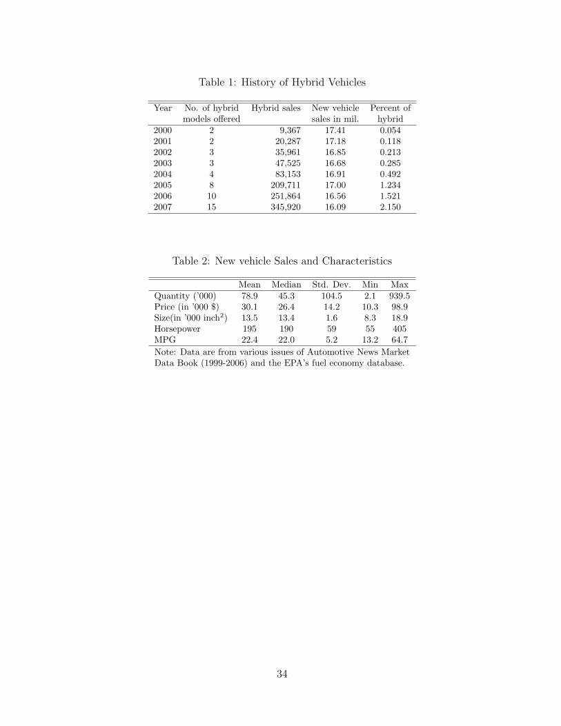
Table 1: History of Hybrid Vehicles

Year No. of hybrid Hybrid sales New vehicle Percent ofmodels offered sales in mil. hybrid

2000 2 9,367 17.41 0.0542001 2 20,287 17.18 0.1182002 3 35,961 16.85 0.2132003 3 47,525 16.68 0.2852004 4 83,153 16.91 0.4922005 8 209,711 17.00 1.2342006 10 251,864 16.56 1.5212007 15 345,920 16.09 2.150

Table 2: New vehicle Sales and Characteristics

Mean Median Std. Dev. Min MaxQuantity (’000) 78.9 45.3 104.5 2.1 939.5Price (in ’000 $) 30.1 26.4 14.2 10.3 98.9Size(in ’000 inch2) 13.5 13.4 1.6 8.3 18.9Horsepower 195 190 59 55 405MPG 22.4 22.0 5.2 13.2 64.7Note: Data are from various issues of Automotive News MarketData Book (1999-2006) and the EPA’s fuel economy database.

34

Table 3: Hybrid Sales and Local Incentives in 2006

MSA Number of Hybrid Percent in total Local incentive Gasolinehouseholds sales vehicle sales (start date) price $

Albany, NY 360,273 737 1.62 Income tax (03/04) 2.70Albuquerque, NM 319,922 763 2.37 Excise tax (07/04) 2.58Atlanta, GA 1,994,938 2,775 1.34 No 2.52Cleveland, OH 1,167,916 1,643 1.16 No 2.51Denver, CO 1,132,085 3,561 3.51 Income tax (01/01) 2.45Des Moines, IA 209,297 438 1.96 No 2.32Hartford, CT 704,130 1,535 2.00 Sales tax (10/04) 2.80Houston, TX 2,197,010 3,132 1.22 No 2.49Lancaster, PA 197,929 318 1.80 No 2.53Las Vegas, NV 713,397 1,340 1.32 No 2.62Little Rock, AR 250,142 436 1.50 No 2.48Madison, WI 185,657 917 4.88 No 2.55Miami, FL 1,706,995 2,322 0.87 HOV (07/03) 2.64Milwaukee, WI 682,896 1,340 1.99 No 2.59Nashville, TN 548,192 752 1.47 No 2.43Phoenix, AZ 1,585,544 3,254 1.53 No 2.51St. Louis, MO 1,100,071 1,526 1.30 No 2.40San Antonio, TX 739,674 1,022 1.25 No 2.41San Diego, CA 1,177,384 4,946 3.40 HOV (08/05) 2.85San Francisco,CA 2,871,199 20,162 7.02 HOV (08/05) 2.87Seattle, WA 1,529,146 5,732 3.82 Sales tax (01/05) 2.70Syracuse, NY 292,717 408 1.15 Income tax (03/04) 2.69

Table 4: Household Demographics and Vehicle Choice

All Households who purchaseNew Car Van SUV Pickup

(1) (2) (3) (4) (5) (6)Household size 2.55 2.88 2.67 3.81 3.02 2.84Renter 0.364 0.211 0.266 0.090 0.147 0.163Children dummy 0.336 0.402 0.328 0.696 0.499 0.352Time to work (minutes) 17.90 20.92 20.49 19.75 19.73 24.00

Income (’000) New vehicle purchase probability< 15 0.0020[15, 25) 0.0440[25, 50) 0.1125[50, 75) 0.1728[75, 100) 0.1972≥ 100 0.2574All households 0.1304Note: Summary statistics are based on households inMSAs from the 2001 National Household Travel Survey.

35

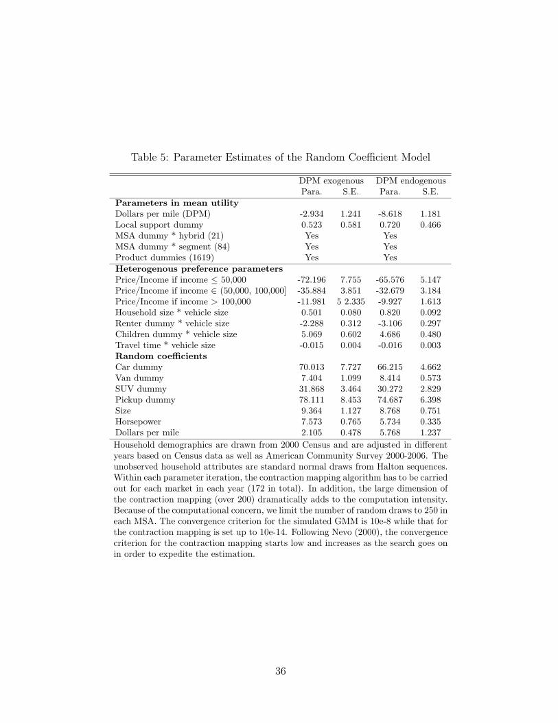
Table 5: Parameter Estimates of the Random Coefficient Model

DPM exogenous DPM endogenousPara. S.E. Para. S.E.

Parameters in mean utilityDollars per mile (DPM) -2.934 1.241 -8.618 1.181Local support dummy 0.523 0.581 0.720 0.466MSA dummy * hybrid (21) Yes YesMSA dummy * segment (84) Yes YesProduct dummies (1619) Yes YesHeterogenous preference parametersPrice/Income if income ≤ 50,000 -72.196 7.755 -65.576 5.147Price/Income if income ∈ (50,000, 100,000] -35.884 3.851 -32.679 3.184Price/Income if income > 100,000 -11.981 5 2.335 -9.927 1.613Household size * vehicle size 0.501 0.080 0.820 0.092Renter dummy * vehicle size -2.288 0.312 -3.106 0.297Children dummy * vehicle size 5.069 0.602 4.686 0.480Travel time * vehicle size -0.015 0.004 -0.016 0.003Random coefficientsCar dummy 70.013 7.727 66.215 4.662Van dummy 7.404 1.099 8.414 0.573SUV dummy 31.868 3.464 30.272 2.829Pickup dummy 78.111 8.453 74.687 6.398Size 9.364 1.127 8.768 0.751Horsepower 7.573 0.765 5.734 0.335Dollars per mile 2.105 0.478 5.768 1.237Household demographics are drawn from 2000 Census and are adjusted in differentyears based on Census data as well as American Community Survey 2000-2006. Theunobserved household attributes are standard normal draws from Halton sequences.Within each parameter iteration, the contraction mapping algorithm has to be carriedout for each market in each year (172 in total). In addition, the large dimension ofthe contraction mapping (over 200) dramatically adds to the computation intensity.Because of the computational concern, we limit the number of random draws to 250 ineach MSA. The convergence criterion for the simulated GMM is 10e-8 while that forthe contraction mapping is set up to 10e-14. Following Nevo (2000), the convergencecriterion for the contraction mapping starts low and increases as the search goes onin order to expedite the estimation.

36

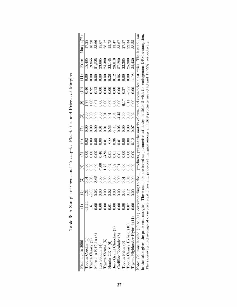
Tab

le6:

ASam

ple

ofO

wn-

and

Cro

ss-p

rice

Ela

stic

itie

san

dP

rice

-cos

tM

argi

ns

Pro

duct

sin

2006

(1)

(2)

(3)

(4)

(5)

(6)

(7)

(8)

(9)

(10)

(11)

Pri

ceM

argi

n(%

)Toy

ota

Cor

olla

(1)

-11.

141.

310.

010.

000.

000.

020.

000.

001.

770.

460.

0015

,485

17.2

5Toy

ota

Cam

ry(2

)1.

61-9

.00

0.08

0.00

0.00

0.03

0.00

0.00

1.06

0.92

0.00

19,8

5518

.28

Mer

cede

sE

Cal

ss(3

)0.

000.

03-3

.65

0.00

0.00

0.00

0.00

0.00

0.01

0.12

0.00

51,8

2533

.66

Kia

Sedo

na(4

)0.

000.

000.

00-7

.00

0.46

0.00

0.01

0.00

0.00

0.00

0.00

23,6

6515

.67

Toy

ota

Sien

na(5

)0.

000.

000.

001.

72-3

.84

0.01

0.01

0.01

0.00

0.00

0.00

24,3

8028

.12

Hon

daC

R-V

(6)

0.01

0.02

0.00

0.02

0.01

-8.8

80.

560.

010.

000.

000.

3622

,145

15.7

8Je

epG

rand

Che

roke

e(7

)0.

000.

000.

000.

020.

010.

36-9

.43

0.04

0.00

0.00

0.12

28,0

1013

.47

Cad

illac

Esc

alad

e(8

)0.

000.

000.

000.

010.

010.

010.

05-4

.45

0.00

0.00

0.06

57,2

8033

.67

Toy

ota

Pri

us(9

)0.

900.

440.

010.

000.

000.

000.

000.

00-6

.17

0.37

0.00

22,3

0527

.57

Toy

ota

Cam

ryH

ybri

d(1

0)0.

070.

120.

040.

000.

000.

000.

000.

000.

11-7

.77

0.00

25,9

0022

.34

Toy

ota

Hig

hlan

der

Hyb

rid

(11)

0.00

0.00

0.00

0.00

0.00

0.12

0.07

0.02

0.00

0.00

-4.0

834

,430

38.5

5N

ote:

Col

umns

labe

led

(1)

to(1

1),c

orre

spon

ding

toth

e11

prod

ucts

,pre

sent

the

mat

rix

ofow

n-an

dcr

oss-

pric

eel

asti

citi

es.

The

last

colu

mn

inth

eta

ble

give

sth

epr

ice-

cost

mar

gins

.T

hese

num

bers

are

base

don

para

met

eres

tim

ates

inTab

le5

wit

hth

een

doge

nous

DP

Mas

sum

ptio

n.T

hesa

les-

wei

ghte

dav

erag

eof

own-

pric

eel

asti

citi

esan

dpr

ice-

cost

mar

gins

amon

gal

l1,

619

prod

ucts

are

-8.4

0an

d17

.72%

,re

spec

tive

ly.

37

Table 7: Robust Analysis: Estimation without Product Dummies

DPM exogenous DPM endogenousPara. S.E. Para. S.E.

Parameters in mean utilityDollars per mile (DPM) -14.914 0.138 -16.445 0.152Local support dummy 0.202 0.159 0.066 0.172Size 0.616 0.350 0.897 0.382Horsepower 2.381 0.157 2.424 0.171Vehicle class dummy (15) Yes YesMSA dummy * hybrid (21) Yes YesMSA dummy * segment (84) Yes YesHeterogenous preference parametersPrice/Income if income ≤ 50,000 -61.214 1.496 -66.556 1.750Price/Income if income ∈ (50,000, 100,000] -39.086 0.750 -42.019 0.901Price/Income if income > 100,000 -11.911 0.601 -11.026 0.728Household size * vehicle size 0.005 0.029 -0.024 0.039Renter dummy * vehicle size -3.234 0.148 -3.453 0.169Children dummy * vehicle size 6.328 0.240 6.951 0.278Travel time * vehicle size -0.044 0.003 -0.048 0.003Random coefficientsCar dummy 53.630 1.256 59.112 1.824Van dummy 4.533 0.849 4.875 0.851SUV dummy 29.451 0.939 31.745 1.064Pickup dummy 57.828 2.328 62.176 2.224Size 8.597 0.319 9.352 0.323Horsepower 6.642 0.202 7.227 0.230Dollars per mile 11.967 0.379 12.802 0.438

38

Table 8: The Effect of Gasoline Price Run-ups from 1999 on Vehicle Prices and Sales

Models in 2006 Price in Price change in % Sales in Sales change in %2006 $ & 90% C.I. 22 MSAs & 90% C.I.

(1) (2) (3) (4)Hybrid ModelsFord Escape Hybrid 29,140 -6.09 [-6.67, -5.33] 3,862 -34.21 [-36.00, -31.82]Honda Civic Hybrid 22,400 -5.59 [-6.34, -4.70] 7,232 -36.82 [-38.55, -33.09]Honda Accord Hybrid 31,540 -4.19 [-4.95, -3.56] 1,210 -21.78 [-22.25, -20.09]Toyota Highlander Hybrid 34,430 -9.56 [-11.14, -8.05] 7,594 -32.13 [-35.21, -28.35]Toyota Prius 22,305 -7.01 [-7.73, -6.08] 26,625 -37.44 [-39.35, -32.71]Non-hybrid ModelsFord Escape 21,745 2.95 [2.39, 3.83] 17,276 25.11 [22.40, 30.36]Honda Civic 17,660 -1.83 [-2.10, -1.46] 60,112 -14.11 [-14.68, -12.24]Honda Accord 21,725 -0.18 [-0.27,-0.07] 69,852 -0.90 [0.20, 1.54]Toyota Highlander 26,535 1.00 [0.74, 1.12] 15,684 2.01 [1.03, 2.92]Toyota Corolla 15,485 -1.43 [-1.56, -1.11] 74,928 -8.03 [-8.78, -6.38]

Note: The table presents the percentage changes in vehicle prices and sales if the gasoline priceshad stayed at the 1999 level. The vehicle sales-weighted average annual gasoline price in the 22MSAs was $2.60 in 2006 compared to $1.53 in 1999, both in 2006 dollars. The brackets give 90%confidence intervals based on parametric bootstrapping.

Table 9: Total Hybrid Sales in 22 MSAs under Different Gasoline Price Scenarios

Year Gas price Sales in Sales change in % with 90% C.I.in 2006 $ 22 MSAs 1999 level $4.00 $6.00

(1) (2) (3) (4) (5)2001 1.75 5,461 -11.47 [-11.67, 11.12] 207.06 [192.63, 238.38] 456.26 [414.02, 540.77]2002 1.54 8,231 2.20 [2.03, 2.38] 205.77 [187.36, 233.10] 430.07 [391.72, 499.63]2003 1.76 9,117 -9.51 [-9.77, 9.31] 157.18 [143.98, 177.60] 364.30 [332.25, 419.95]2004 2.01 17,732 -18.62 [-19.94, -16.17] 110.16 [101.65, 131.61] 268.39 [239.08, 304.60]2005 2.41 43,658 -23.69 [-26.64, -20.99] 64.59 [ 60.69, 73.18] 165.47 [147.15, 189.71]2006 2.60 59,059 -36.60 [-38.04, -32.41] 64.55 [56.55, 76.02] 183.24 [159.10, 216.30]Note: Column (1) lists vehicle sales-weighted average annual gasoline prices in the 22 MSAs. Column(3) presents the percentage changes in total hybrid vehicle sales with 90% confidence intervals when gasprices were assumed to be at the 1999 level in each of the MSAs. The sales-weighted average gasolineprice in the 22 MSAs was $1.53 in 1999.

39

Table 10: The Effect of Tax Incentives on Selected Hybrid Models

Observed Incentives Without IncentivesPrice Sales in Subsidy Price change in % Sales change in %

(in 2006 $) 22 MSAs in 2006$ with 90% C.I. with 90% C.I.(1) (2) (3) (4) (5)

2005 HybridFord Escape 28,330 2,918 371 -0.67 [-0.69, -0.66] -0.62 [-1.00, -0.26]Honda Civic 20,815 4,836 471 -0.82 [-0.84, -0.79] -3.86 [-4.19, -3.39]Honda Accord 31,489 3,146 527 -0.69 [-0.70, -0.68] -1.55 [-1.91, -1.09]Toyota Highlander 33,476 3,366 450 -0.65 [-0.66, -0.65] -0.38 [-0.74, 0.11]Toyota Prius 22,106 25,528 522 -0.89 [-0.92, -0.86] -2.27 [-2.44, -2.01]2006 HybridFord Escape 29,140 3,862 1,960 -3.25 [-3.38, -3.16] -17.48 [-18.69, -15.98]Honda Civic 22,400 7,232 1,947 -3.11 [-3.20, -3.07] -22.31 [-23.89, -20.51]Honda Accord 31,540 1,210 624 -0.86 [-0.88, -0.85] -4.41 [-4.99, -3.79]Toyota Highlander 34,430 7,594 2,172 -2.94 [-2.97, -2.93] -10.68 [-12.38, -8.72]Toyota Prius 22,305 26,625 2,617 -4.36 [-4.52, -4.29] -24.60 [-25.56, -23.17]Note: Column (3) presents the average tax benefit received by the buyers of each hybrid model inthe 22 MSAs. The 90% confidence intervals for simulation results in brackets are obtained usingparametric bootstrapping.

Table 11: The Effect of Tax Incentives on Hybrid Adoption from 2001 to 2006

Observed Incentives Without Incentives Doubled IncentivesYear Hybrid Sales Subsidy Sales change in % Subsidy Sales change in %

in 22 MSAs in 2006 $ with 90% C.I in 2006 $ with 90% C.I(1) (2) (3) (4) (5)

2001 5,461 611 -4.51 [-4.92, -4.12] 1,233 4.96 [4.54, 5.41]2002 8,231 572 -4.79 [-5.15, -4.39] 1,154 4.89 [4.54, 5.28]2003 9,117 529 -4.32 [-4.63, -4.02] 1,048 4.01 [3.73, 4.35]2004 17,732 521 -4.49 [-4.71, -4.11] 1,030 4.24 [3.86, 4.49]2005 43,658 473 -3.58 [-3.78, -3.23] 943 3.46 [3.15, 3.68]2006 59,059 2,276 -19.75 [-20.91, -18.08] 4,754 22.94 [20.55, 24.45]

40

Table 12: Policy Effects on Gasoline Consumption and CO2 Emissions

New Vehicle New Vehicle Sales Gas Consumption CO2 EmissionsMPG in ’000 in mil. barrels in mil. tons(1) (2) (3) (4)

Observed 23.19 2467.92 456.04 191.54Changes under Different Policies

Income Tax CreditWithout -0.10 [-0.10, -0.09] -0.65 [-0.78 -0.48] 1.80 [1.73, 1.88] 0.76 [0.73, 0.79]Doubled 0.12 [0.11, 0.13] 0.81 [0.71, 1.02] -2.15 [-2.28, -1.98] -0.90 [-0.96, -0.03]

Gasoline Tax Increase$0.10 0.10 [0.09, 0.11] -37.36 [-39.31 -36.27] -8.83 [-9.31 -8.50] -3.70 [-3.91 -3.57]$0.25 0.29 [0.27, 0.30] -98.23 [ -103.44, -96.05] -23.51 [ -24.44 -22.88] -9.87 [-10.27, -9.61]$1.00 1.01 [0.92, 1.08] -309.54 [-323.27, -297.15] -73.84 [-76.83, -70.64] -31.01 [-32.27, -29.67]Note: The numbers in the table are for 2006 cohort of new vehicles sold in the 22 MSAs. Both total gasolineconsumption and CO2 emissions are calculated for the lifetime of these vehicles (15 years with 12,000 milestraveled per year).

Table 13: Comparison of the Tax Credit Program with a Rebate Program

Average MPG Total Subsidy in 2006 $millionin 22 MSAs with 90% C.I.

Baseline: Current Tax CreditsTax Credit Program 23.19 134.43 [134.13, 134.72]Rebate Program 23.19 113.60 [112.50, 115.91]Difference 0 -20.83 [-21.87, -18.59] (-15.5%)

Baseline: Doubling Tax CreditsTax Credit Program 23.31 346.08 [336.99, 352.52]Rebate Program 23.31 260.21 [255.14 264.93]Difference 0 -85.87 [-89.90 -80.01] (-24.8%)

Table 14: Robustness Analysis: Vehicle Prices Constant

Year Hybrid Sales Sale Change in % with 90% C.I.in 22 MSAs Gas Price at 1999 Level Without Incentives

(1) (2) (3)2001 5,461 -23.04 [-23.40, -22.40] -8.54 [-9.30, -7.77]2002 8,231 4.47 [4.10, 4.85] -8.96 [-9.71, -8.17]2003 9,117 -19.12 [-19.69, -18.64] -8.08 [-8.68, -7.46]2004 17,732 -35.62 [-38.09, -31.14] -8.49 [-8.94, -7.81]2005 43,658 -44.63 [-50.22, -39.59] -7.03 [-7.45, -6.32]2006 59,059 -61.96 [-65.05, -56.13] -31.40 [-33.05, -29.28]Note: Vehicle prices are held constant in the simulations.

41