Asymmetric Pass-Through in U.S. Gasoline Prices

Matthew Chesnes1

Federal Trade Commission, Bureau of Economics, 600 Pennsylvania Avenue, N.W., Washington DC, 20580

Abstract

This paper presents new evidence of asymmetric pass-through, the notion that upward cost shocksare passed through faster than downward cost shocks, in U.S. gasoline prices. Much of the extant lit-erature comes to seemingly contradictory conclusions about the existence and causes of asymmetry,though the differences may be due to different aggregation (both over time and geographic markets)and the use of different price series including crude oil, wholesale, and retail gasoline prices.

I utilize a large and detailed dataset to determine where evidence of a pass-through asymmetryexists, and how it depends on the aggregation and price series chosen by the researcher. Using theerror correction model, I find evidence of pass-through asymmetry based on spot, rack and retailprices, though the largest effect is found in the rack to retail relationship. I find more asymmetryin branded prices compared with unbranded prices, consistent with a consumer search explanationfor asymmetry. However, I also find evidence consistent with explanations based on market poweras the magnitude of asymmetry is positively associated with retail concentration. On average, retailprices rise three to four times as fast as they fall.

Keywords: Gasoline prices, Cost pass-through, Asymmetric adjustment

1. Introduction

There is a large literature analyzing the cost to price pass-through in industries ranging fromautomobiles (Gron and Swenson (1982)), to cheese products (Kim and Cotterill (2008)), to the beefindustry (Goodwin and Holt (1999)). The literature has not only focused on the ability of firmsto successfully capture rents when input costs change, but also on how the rate of pass-throughvaries when the costs increase versus decrease. Peltzman (2000) analyzes over 200 consumer andproducer products and find asymmetric adjustment in two-thirds of the products. Similarly, Meyeret al. (2004) surveys the literature and finds that symmetric adjustment is rejected in about one-half of the cases. Much of the extant literature comes to seemingly contradictory conclusions aboutthe existence and causes of this phenomenon, though the differences may be due to different datasources, price series, aggregation over time and across geographic areas, as well as misspecifiedmodels. In this paper, I examine the dynamics of pass-through in gasoline prices using a detaileddataset available at a high frequency, across many cities, and at several price levels in the verticaldistribution process for gasoline.

1Email: mchesnes@ftc.gov. Web: http://www.chesnes.com. The opinions expressed here are those of the authorand not necessarily those of the Federal Trade Commission or any of its Commissioners. I thank Michael Noel, MatthewLewis, Chris Taylor, Louis Silvia, David Meyer, Doug Herman, and participants at the 2010 International Industrial Organi-zation Conference for their suggestions and comments. Elisabeth Murphy and Elizabeth Miles provided excellent researchassistance. All remaining errors are my own.

Preprint submitted to The Energy Journal February 3, 2015

Particularly in the gasoline industry, this asymmetric phenomenon is known as rockets and feath-ers, reflecting the fact that retail prices tend to increase quickly when costs (say, wholesale gasolineprices) rise, but drift down slowly when they fall.2 Pass-through in the gasoline industry has beenthe focus of many studies for several reasons. Gasoline is a fairly homogeneous product and bothretail and intermediate wholesale prices are relatively transparent compared with other industries.3

Much of the variation in gasoline prices is driven by the price of crude oil, the key input into gaso-line.4 Crude oil is traded on a world market and the price is also transparent to market players and toconsumers. In spite of the transparency of prices, there are dynamics present in the gasoline industrythat are difficult to explain with competitive or oligopolistic economic models.

The literature on rockets and feathers dates back to at least 1991 when Robert Bacon foundevidence of an asymmetric response in gasoline prices in the UK. Since that time, others have foundevidence of the phenomenon including Borenstein, Cameron, and Gilbert (1997, hereafter BCG),Ye et. al. (2005), Deltas (2008), Tappata (2009) and Lewis (2011). These studies all utilize someform of an error correction model (outlined below) and consider some combination of crude oilprices, wholesale prices (rack or spot), and retail gasoline prices. They also vary by the geographythey consider and how the data are aggregated over time. There are also several papers that, due toeither a different data source or model, find no evidence of an asymmetric price response includingGodby (2000) and Gautier and Le Saout (2012). Bachmeier and Griffin (2003) test the results inBCG using daily data and a different methodology and find no evidence of asymmetric adjustment,however they only focus on the transmission of crude oil to spot gasoline prices.

If it exists, there is little consensus on what causes an asymmetric response. BCG offer threepotential explanations for asymmetric adjustment: focal-point pricing as a form of market power,inventory adjustment frictions in the face of positive and negative demand shocks, and differencesin consumer search patterns when prices are rising and falling. Deltas (2008) and Verlinda (2008)look at how the asymmetric response varies with the level of retail market power and find moreasymmetry in markets with relatively more retail market power.5

Lewis (2011) and Tapatta (2009) posit that consumer search behavior could be causing the asym-metric response. If consumers are more likely to search for a low price when prices are rising orexpected to rise, then competition will be fierce when costs are rising and margins tight. However,if prices are falling, consumers may search less and this provides retailers with short-term marketpower and allows them to slowly lower prices and increase their margins. Evidence of this explana-tion could be found in the difference in asymmetry between branded and unbranded gasoline prices.If consumers who purchase unbranded gasoline tend to search more intensively than branded cus-tomers who are loyal to a specific brand, cost shocks to unbranded rack prices would be passed on

2The production and distribution of gasoline is just one part of the petroleum industry, which produces a whole range ofrefined products. The rockets and feathers literature has focused primarily on gasoline prices.

3Rack prices for wholesale gasoline are observable and in 2009, rack sales accounted for 60% of the total gasoline suppliedin the U.S. See http://tonto.eia.doe.gov/dnav/pet/pet_cons_refmg_c_nus_epm0_mgalpd_a.htm and http:

//tonto.eia.doe.gov/dnav/pet/pet_cons_psup_dc_nus_mbbl_m.htm. The rest is sold to lessee-dealer stations at(unobserved) dealer-tank-wagon (DTW) prices and via transfer prices to refiner-operated stations.

4See The Federal Trade Commission, “Gasoline Price Changes: The Dynamics of Supply, Demand and Competition,”2005.

5In Deltas, the average markup observed in the market over his sample period serves as a proxy for market power. It istempting to assume that markets in which firms face less competition will feature firms quickly passing on cost increasesto consumers, and only slowly (or possibly never) passing on cost savings. Markets with many competing firms shouldfeature perfect pass-through. For industry-wide cost changes, this is generally true, however the opposite results when thecost change is firm-specific. Bulow and Pfleiderer (1983) show that firm-specific cost changes are more completely passedthrough the less competitive is the market. (See also, Ten Kate and Niels (2005).) The reason is that when faced with a costdecrease, say, firms with a greater market share will benefit relatively more from the increase in quantity demanded, whichmore than offsets the lower revenue from passing on the cost decrease in the form of lower prices.

2

more quickly to retail prices.The Edgeworth price cycle model of Maskin and Tirole (1988) may also explain the dynamics.

They show that competition may lead to relatively slow price undercutting down to cost and a rapidrise or resetting of the cycle initiated by a single firm and quickly followed by all its competitors.Several studies have found evidencing of price cycles in gasoline markets (see Eckert (2002), Noel(2007, 2009), Lewis and Noel (2011), and Zimmerman et al. (2013)). While price cycle models donot deal directly with the response of prices to changes in costs, cycles and asymmetric pass-throughmay be related. Lewis and Noel (2011) show that cost shocks are passed through faster in marketsthat feature price cycles. However, the speed of pass-through may be unrelated to the asymmetricresponse to positive and negative cost shocks. Pass-through rates may be fast, though asymmetric,so cycling cities may show evidence of asymmetric pass-through even if the speed of pass-throughis faster than in non-cycling cities.

This paper is similar to BCG in that I analyze several different prices (crude oil, spot gasoline,rack, and retail prices) over a long period of time. However, unlike BCG who use weekly and bi-weekly data from the Lundberg Survey, I have access to daily data on all prices. I also avoid amodeling assumption by BCG (discussed below) which was questioned by Bachmeier and Griffin(2003) and instead use a more standard approach. I also consider how asymmetry varies acrossdifferent U.S. cities, between branded and unbranded prices, and how asymmetric pass-through iscorrelated with market concentration and the existence of price cycles.

I find evidence of asymmetry in the crude oil to gasoline spot price, the spot to rack, and therack to retail price relationships.6 The rack to retail relationship shows the strongest asymmetry atboth the city and national level. On average, retail prices rise three to four times as fast as theyfall. Asymmetry varies significantly across cities with the strongest rack to retail asymmetry in SaltLake City, Louisville (Indiana) and Cleveland. New York shows the least asymmetric pass-through.Estimates based on weekly data show more asymmetric pass-through as retail prices are predictedto increase faster following a cost (rack price) increase and fall slower following a cost decrease.Branded gasoline features significantly more asymmetry compared with unbranded gasoline in re-sponse to changes in the rack price, consistent with the consumer search explanation for asymmetricpass-through. Computing the impact of asymmetric pass-through over time shows significant dif-ferences by year, though on average, retail prices would be about 2.45 cents per gallon (cpg) lowerif they fell as quickly as they rose.

Finally, I find that cities that show more asymmetric pass-through tend to feature more pricecycling and have a faster overall speed of pass-through. I also find evidence that asymmetry ispositively related to market concentration. The overall brand-level Herfindahl-Hirschman Index isabout 14% higher for cities in the top quartile of asymmetry relative to the bottom quartile.

The paper proceeds as follows. In section 2, I outline the model that I employ and specificationtests are run to justify its use. I discuss the data and provide basic descriptive statistics in section3 and present the results of my model in section 4, including asymmetric pass-through results fordifferent geographic areas, at different levels of time aggregation, and for different products. Ialso present city-specific factors that may be related to the magnitude of asymmetric pass-through.Section 5 concludes.

6It is important to note that the model predicts complete pass-through of both positive and negative cost shocks after someperiod of time, typically around two weeks. Asymmetric pass-through generally occurs in the first week after the cost shockand after which, pass-through of positive and negative shocks is statistically indistinguishable.

3

2. Model

I estimate an error correction model (ECM) frequently used in the literature, though in variousforms (e.g., Bachmeier and Griffin (2003)). I estimate the model individually for each city (metroarea)7 and for a national specification that allows for different price levels and markups in eachcity. The latter regression measures the average pass-through rate across all cities, while allowingthe long-term relationship to vary by city. I allow for a difference in the pass-through of positiveand negative upstream price changes. While I estimate the model for several pairs of upstream anddownstream prices, for simplicity, the following is the rack to retail pass-through model for a givencity:

∆Retailt =L+1

∑i=0

β+1i ∆

+Rackt−i +L−1

∑i=0

β−1i ∆−Rackt−i (1)

+L+2

∑i=1

β+2i ∆

+Retailt−i +L−2

∑i=1

β−2i ∆−Retailt−i

+ β+3 (Retailt−1− γ0− γ1Rackt−1)︸ ︷︷ ︸

z+t−1

+ β−3 (Retailt−1− γ0− γ1Rackt−1)︸ ︷︷ ︸

z−t−1

+εt .

Note ∆Retailt−i = Retailt−i−Retailt−(i−1). Lag lengths are determined by minimizing the BayesianInformation Criterion (BIC):

BIC = K ∗ log(N)+N ∗ [Log(RSS/N)], (2)

where K is the number of parameters to be estimated, N is the number of observations, and RSS= ε ′εfrom equation 1. I could allow the lag lengths to vary separately for positive and negative changes aswell as for rack and retail prices. However, since determining the optimal lag lengths for each priceseries, versus using a fixed (and equal) lag length for all, does not affect the qualitative results, inthe analysis below I fix the lag length at 21 days in all regressions.8 This also allows me to compareregressions across cities and over time since I will utilize the same specification in each.

The expression zt−1 = Retailt−1− γ0− γ1Rackt−1 is the error correction term, and it capturesthe long-run relationship between the upstream and downstream prices. β

+3 and β

−3 should both be

negative: if retail prices are above their equilibrium level (zt−1 > 0), retail prices should fall and ifthey are below the level predicted by the rack price (zt−1 < 0), retail prices should rise.

Following the two-step method proposed by Engle and Granger (1987), I estimate γ0 and γ1 byrunning OLS on the following equation:

Retailt−1 = γ0 + γ1Rackt−1 + zt−1. (3)

7Most of the metro areas in my sample are major cities. Some cities near state borders are split across state lines, sofor example, Louisville, KY and Louisville, IN are separate metro areas. See figure A1 for an example. This is importantbecause often different types of gasoline (e.g., conventional, RFG, and California Air Resources Board (CARB) gasoline)are sold in different states.

8The lag length is also three in the weekly specifications.

4

The residuals, zt−1, are then inserted directly into the model.9 BCG estimate the long-term relation-ship in the same step as the rest of the parameters and instrument for the upstream prices to controlfor possible endogeneity. As outlined in Bachmeier and Griffin (2003), this may lead to problemswith the resulting estimates.10 Once I obtain the residuals, I can estimate equation 1 by OLS. 11

Asymmetric adjustment of downstream prices to changes in an upstream cost (such as a whole-sale price) is generally divided into two forms: amount asymmetry and pattern asymmetry. Amountasymmetry occurs when the aggregate change over a period of time is different when costs are risingversus when they are falling. In terms of the model parameters, amount asymmetry would be of theform:

L+1

∑i=0

β+1i 6=

L−1

∑i=0

β−1i . (4)

However, this cannot exist over the long term since upstream and downstream prices do not tend todrift apart.

Pattern asymmetry involves differences in the relative speed of pass-through. As an example,one may find evidence of pattern asymmetry if a 10% increase in wholesale prices leads to a 10%increase in retail prices after one week, but an equivalent decrease in wholesale prices leads to onlya 5% decline in retail prices after one week and the full 10% after two weeks. Pattern asymmetrycould be found if any one of the following three conditions are met:

β+1i 6= β

−1i for some i (5)

|β+3i | 6= |β−3i | (6)L+

1 6= L−1 or L+2 6= L−2 . (7)

The asymmetry in equation 5 is the one commonly analyzed in the literature. While the aggregatepass-through should be the same for positive and negative rack price changes, the pattern of pass-through may be different. If any of the coefficients on the same lag are different, this is evidenceof pattern asymmetry. The coefficients on the first lag, β

+1,1 and β

−1,1, are particularly important

because they measure the contemporaneous speed of pass-through, assuming the model could beapproximated as a first-order difference equation. However, to fully assess the impact of asymmetricadjustment on the downstream price, a full impulse response function will be estimated taking intoaccount all lags of the upstream and downstream price. In principal, any difference in the coefficientsis evidence of some form of pattern asymmetry, but the rockets and feathers type of asymmetryimplies β

+1i > β

−1i for least one lag.

The second pattern asymmetry (noting again that β3 should be negative reflecting mean-reversion)involves the speed at which relative prices return to their long-term equilibrium levels. We have evi-dence of the rockets and feathers type of asymmetry if this mean reversion is slower (closer to zero)when retail prices are above their long-term levels and faster when retail prices should be adjustingupwards toward their long-term levels (i.e., |β+

3 |< |β−3 |).

Finally, if I allowed the BIC-optimum lag lengths to vary for positive and negative changes,

9Since the two series are cointegrated, the OLS regression yields super-consistent estimates of the parameters. Theestimates can then be inserted into the model as if they were known parameters.

10BCG run a two-stage least squares regression and instrument for the upstream price with the crude oil price in Englandand forward prices of crude oil in the U.S. However, while they reject the null that there is no endogeneity in the prices, their2SLS and OLS estimates are very similar.

11For the national-level specification, I estimate equation 3 separately for each city and then substitute the residuals(stacked, city by city), into equation 1.

5

further evidence of pattern asymmetry is obtained if the optimal lag lengths are different. Thoughthis is often the case, I fix the lag lengths and focus most of my attention on the asymmetries inequations 5 and 6.

3. Data and Descriptive Statistics

I combine two datasets to perform the analysis. Spot prices are available from Reuters viathe Energy Information Administration (EIA) and rack and retail price data are from the Oil PriceInformation Service (OPIS). All data are available daily (weekends and missing values discussedbelow) from 2000 through 2013 though some series are not available for the entire period. Summarystatistics are provided in tables 1, 2, and 3.

Spot prices include the price of West Texas Intermediate (WTI) crude oil at Cushing, Oklahomaand Brent crude oil produced in the North Sea region. I also obtain the conventional and reformu-lated gasoline (RFG) spot prices on the Gulf Coast12 along with another conventional spot at NewYork Harbor and RFG/RBOB13 spot price for Los Angeles. Spot prices are reported as of the closeof day, Monday through Friday.

Table 1: Daily Spot Prices (Cents per Gallon)

Date MarginSpot Price N Min Mean Max Std Dev Range Over WTIGulf - Conventional 3,478 44.00 173.09 475.96 80.14 1/00-12/13 23.50Gulf - RFG 3,478 26.05 176.93 452.91 79.93 1/00-12/13 27.34NY - Conventional 3,478 46.75 175.96 366.50 81.67 1/00-12/13 26.37LA - RFG/RBOB 3,478 47.00 192.73 417.70 81.03 1/00-12/13 43.14Brent 3,478 39.31 154.52 342.74 79.56 1/00-12/13 4.93WTI 3,478 41.67 149.59 345.98 68.87 1/00-12/13 0.00

I use rack prices from OPIS for 20 U.S. cities. These rack prices are for the type of gasolineused in each city since many cities utilize different types of gasoline (conventional, RFG, etc.). Insome cases, rack prices for different types of gasoline are reported in the same city. In these cases,I use the rack price that corresponds to the type of gasoline that is used in each retail market area.For example, the Fairfax, VA rack reports both conventional and RFG prices. Since I observe retaildata for stations in Washington, DC, as well as the Virginia, Maryland, and West Virginia suburbsof DC, I match the RFG rack price to DC, VA, and MD since each uses primarily RFG, while theWV retail prices are matched to the conventional rack since that area primarily uses conventionalgasoline. Rack prices are reported as of 9AM, Monday through Saturday and are available for bothbranded and unbranded products.14

12The Gulf Coast RFG price becomes Gulf RFG with Ethanol in June 2006.13RBOB is short for Reformulated Blendstock for Oxygenate Blending. The Los Angeles RFG price is replaced with the

RBOB spot price in November 2003.14For racks that report multiple prices for different types of RFG or different types of conventional gasoline on the same

day, the lowest price quote is selected.

6

Table 2: Daily Branded Rack Prices (Cents per Gallon)

Date MarginRack N Min Mean Max Std Dev Range Over WTIAtlanta (Conventional) 4,298 50.64 182.75 354.29 81.37 1/00-12/13 33.08Boston (RFG) 4,365 56.15 187.77 362.22 82.29 1/00-12/13 38.54Chicago (RFG) 4,365 61.64 190.28 366.60 81.16 1/00-12/13 41.10Cleveland (Conventional) 4,365 54.22 183.90 359.30 80.55 1/00-12/13 34.66Dallas (RFG) 4,365 54.47 184.81 356.63 80.82 1/00-12/13 35.62Denver (Conventional) 4,365 52.23 183.68 364.76 80.80 1/00-12/13 34.65Detroit (Conventional) 4,365 52.02 184.43 361.20 81.53 1/00-12/13 35.26Fairfax (Conventional) 4,365 53.49 185.84 356.28 81.68 1/00-12/13 36.64Fairfax (RFG) 4,365 51.22 180.84 351.70 80.28 1/00-12/13 31.62Houston (RFG) 4,364 52.44 182.77 355.03 81.14 1/00-12/13 33.53Los Angeles (CARB) 4,062 59.28 207.39 392.91 77.66 12/00-12/13 52.72Louisville (Conventional) 4,348 52.58 183.23 355.70 80.08 1/00-12/13 33.74Louisville (RFG) 3,563 84.89 216.85 376.64 74.38 7/02-12/13 48.72Miami (Conventional) 4,361 50.98 182.11 353.51 81.44 1/00-12/13 32.97Minneapolis (Conventional) 4,363 51.41 184.76 363.60 79.61 1/00-12/13 35.60New Orleans (Conventional) 4,365 50.02 178.71 350.88 80.26 1/00-12/13 29.52Newark (RFG) 2,374 98.89 245.14 355.16 54.72 5/06-12/13 44.60Phoenix (Conventional) 4,365 61.61 195.62 366.58 79.66 1/00-12/13 46.61Salt Lake City (Conventional) 4,364 59.11 188.71 367.52 80.99 1/00-12/13 39.83San Francisco (CARB) 4,158 59.23 202.17 380.51 77.82 1/00-12/13 49.33Seattle (Conventional) 4,365 56.21 190.64 364.57 80.77 1/00-12/13 41.60St Louis (Conventional) 4,357 52.51 182.27 355.41 80.00 1/00-12/13 33.14St Louis (RFG) 4,365 57.92 188.11 364.79 79.10 1/00-12/13 38.97

Some racks service multiple states with different types of wholesale gasoline. The Fairfax, VA rack sells RFGto stations in DC, MD, and VA, while it sells conventional gasoline to stations in WV. Similarly Louisville andSt. Louis sell conventional gasoline to stations in IN and IL and RFG to stations in KY and MO respectively.

Finally, I utilize pre-tax retail price data from OPIS for the 27 retail metro areas all within the20 cities for which I have rack prices. Retail prices are (usually) end of the day prices as they arerecorded from the last swipe of a consumer’s “fleet-card” on a given day.15 OPIS averages all theprices they receive each day (at most one from each station) to determine the price for the metroarea. After 2001, the prices are reported every day of the week. OPIS samples over 100,000 stationseach day and covers branded and unbranded stations. As shown in table 3, (pre-tax) retail pricesvaried significantly during this period from 53 cents per gallon to over $4 per gallon. The Seattlemetro area had the highest average margin (retail less rack price) over the sample period while NewOrleans had the lowest average margin.

15See http://www.opisretail.com/methodology.html for more information on OPIS’s retail data. More than one-half of the stations in the OPIS sample report a price each day, though the sample of stations may change from day today.

7

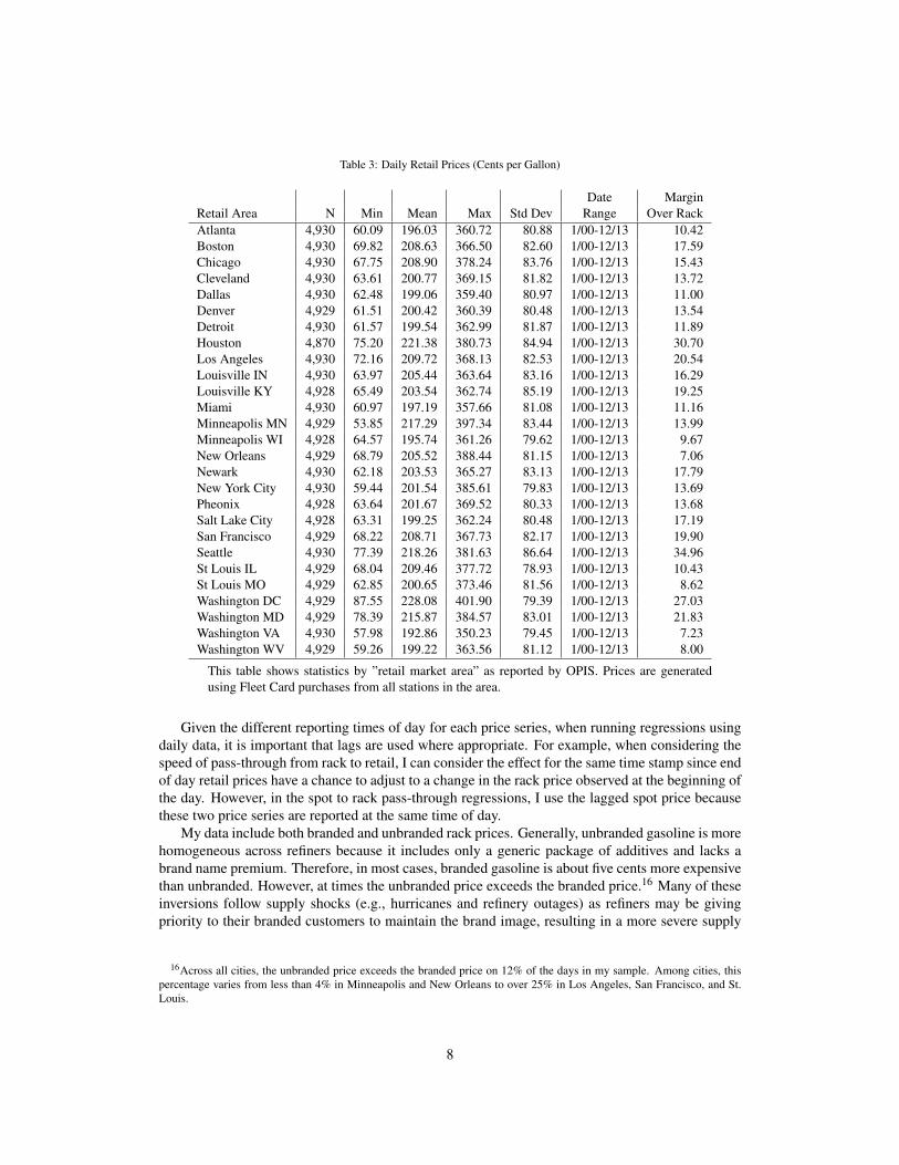
Table 3: Daily Retail Prices (Cents per Gallon)

Date MarginRetail Area N Min Mean Max Std Dev Range Over RackAtlanta 4,930 60.09 196.03 360.72 80.88 1/00-12/13 10.42Boston 4,930 69.82 208.63 366.50 82.60 1/00-12/13 17.59Chicago 4,930 67.75 208.90 378.24 83.76 1/00-12/13 15.43Cleveland 4,930 63.61 200.77 369.15 81.82 1/00-12/13 13.72Dallas 4,930 62.48 199.06 359.40 80.97 1/00-12/13 11.00Denver 4,929 61.51 200.42 360.39 80.48 1/00-12/13 13.54Detroit 4,930 61.57 199.54 362.99 81.87 1/00-12/13 11.89Houston 4,870 75.20 221.38 380.73 84.94 1/00-12/13 30.70Los Angeles 4,930 72.16 209.72 368.13 82.53 1/00-12/13 20.54Louisville IN 4,930 63.97 205.44 363.64 83.16 1/00-12/13 16.29Louisville KY 4,928 65.49 203.54 362.74 85.19 1/00-12/13 19.25Miami 4,930 60.97 197.19 357.66 81.08 1/00-12/13 11.16Minneapolis MN 4,929 53.85 217.29 397.34 83.44 1/00-12/13 13.99Minneapolis WI 4,928 64.57 195.74 361.26 79.62 1/00-12/13 9.67New Orleans 4,929 68.79 205.52 388.44 81.15 1/00-12/13 7.06Newark 4,930 62.18 203.53 365.27 83.13 1/00-12/13 17.79New York City 4,930 59.44 201.54 385.61 79.83 1/00-12/13 13.69Pheonix 4,928 63.64 201.67 369.52 80.33 1/00-12/13 13.68Salt Lake City 4,928 63.31 199.25 362.24 80.48 1/00-12/13 17.19San Francisco 4,929 68.22 208.71 367.73 82.17 1/00-12/13 19.90Seattle 4,930 77.39 218.26 381.63 86.64 1/00-12/13 34.96St Louis IL 4,929 68.04 209.46 377.72 78.93 1/00-12/13 10.43St Louis MO 4,929 62.85 200.65 373.46 81.56 1/00-12/13 8.62Washington DC 4,929 87.55 228.08 401.90 79.39 1/00-12/13 27.03Washington MD 4,929 78.39 215.87 384.57 83.01 1/00-12/13 21.83Washington VA 4,930 57.98 192.86 350.23 79.45 1/00-12/13 7.23Washington WV 4,929 59.26 199.22 363.56 81.12 1/00-12/13 8.00

This table shows statistics by ”retail market area” as reported by OPIS. Prices are generatedusing Fleet Card purchases from all stations in the area.

Given the different reporting times of day for each price series, when running regressions usingdaily data, it is important that lags are used where appropriate. For example, when considering thespeed of pass-through from rack to retail, I can consider the effect for the same time stamp since endof day retail prices have a chance to adjust to a change in the rack price observed at the beginning ofthe day. However, in the spot to rack pass-through regressions, I use the lagged spot price becausethese two price series are reported at the same time of day.

My data include both branded and unbranded rack prices. Generally, unbranded gasoline is morehomogeneous across refiners because it includes only a generic package of additives and lacks abrand name premium. Therefore, in most cases, branded gasoline is about five cents more expensivethan unbranded. However, at times the unbranded price exceeds the branded price.16 Many of theseinversions follow supply shocks (e.g., hurricanes and refinery outages) as refiners may be givingpriority to their branded customers to maintain the brand image, resulting in a more severe supply

16Across all cities, the unbranded price exceeds the branded price on 12% of the days in my sample. Among cities, thispercentage varies from less than 4% in Minneapolis and New Orleans to over 25% in Los Angeles, San Francisco, and St.Louis.

8

reduction for unbranded gasoline. Whatever the cause, below I investigate the asymmetric responsefor branded and unbranded fuel separately.

In addition to data from EIA and OPIS, I also gather information on each city in the sampleto assess factors that may be associated with more or less asymmetric pass-through. Some factors,such as the degree of price cycling and the speed of cost pass-through can be calculated using theEIA data. In addition, I calculate brand-level retail market concentration for each city based on salesdata from New Image Marketing Research Corporation.17 These data provide brand-level sales for22 of the 27 cities in my sample for a single year between 1998 and 2001, which is around the startof my sample period.

3.1. Data Issues

Before focusing on the results, there are a few issues with the data that need to be addressed. Irun my regressions at both a daily and a weekly frequency. Weekly data is generated both as thesimple average of the daily series and by choosing a specific day of each week.18 Using the dailyaverage means that sometimes the average is over five days, other times six days, four days, etc.Using the weekly price series based on a particular day of the week avoids this issue, though it turnsout that the estimates using either method are almost identical.

Due to weekends, holidays, etc, there are some missing values in the daily data. Since the re-gression equations involve the contemporaneous and lagged change in prices, it is important to makeconstant the time over which the change is calculated. For over 99.9% of the daily observations, thedifference in days between observations is three or less (82.8% of the observations are adjacent).In the results presented in the next section, I linearly interpolate the prices if one or two days aremissing between observations and I drop any observation where the change in price is over three ormore days. The resulting dataset contains daily observations where the change in prices is alwaysover exactly one day.

For robustness, I also consider two alternative methodologies:

1. do not interpolate and drop changes over three or more days;2. do not interpolate and do not drop multi-day changes.

Each of these alternatives lead to qualitatively similar results. The estimates themselves change onlyslightly and are never statistically different from each other. For example, using the branded rack-to-retail national specification, the positive and negative contemporary coefficients (β+

1,1 and β−1,1)

using the baseline algorithm are 0.23 and 0.08 respectively. They change slightly to 0.23 and 0.07using alternative one, and 0.24 and 0.07 using alternative two.

Finally, at one time the spot price for RFG was for reformulated gasoline blended with MTBE,which has now been banned in most states.19 It has been replaced by the RBOB spot price, which isRFG that will eventually get blended with an oxygenate (typically ethanol). For the LA spot price,there is some overlap in the two series so I create a complete spot price series for RFG using the oldRFG spot for the early part of the sample and switching to the RBOB spot as soon as it is reported.The two prices are similar to each other during the overlap period.20 For the Gulf Coast, there is nooverlap (the RFG spot ends on one day and the RBOB spot begins being reported on the very nextday) so I concatenate the two series to form my complete Gulf Coast RFG spot price. However, the

17See http://www.nimresearch.com/.18My algorithm selects the price on Wednesday in almost all weeks, though selects the price on Thursday in the few weeks

when there is no reported Wednesday price.19In some states the liability protection has been removed so refiners are reluctant to use it.20A simple regression of the RFG spot on the RBOB spot during the overlap yields a slope coefficient of 0.95.

9

RBOB price on its first day reported is 38 cents higher than the RFG spot on the previous day.21

For robustness, I have run the models only using dates where I observe the RFG spot price and theresults are qualitatively similar.

4. Results

Before analyzing the results, it is important to test for stationarity of the regressors. I run aDickey Fuller (DF) test on each price series, which show that all have a unit root so first differencingis necessary. I then run the Johansen test on each set of price series together and confirm thatthe upstream and downstream price series are cointegrated (i.e., the residuals from the long-runregression equation 3 are stationary).22 Therefore, estimating the long-term relationship in the firststage provides super-consistent estimates that can be entered into the model directly. Durbin Watsontests for autocorrelation correlation are also run and fail to reject the hypothesis that there is noautocorrelation in the residuals for each model.

I divide the results into several sections which consider the differences in pattern asymmetryamong different price relationships, across cities and in the national regression, by the time aggre-gation of the data, for branded versus unbranded wholesale gasoline, and over time. I show formalF-tests of pattern asymmetry for each type of model and provide evidence of city-specific factorsthat are correlated with the magnitude of asymmetry.

4.1. Price Relationships

I investigate pass-through asymmetry for combinations of the crude oil price, the gasoline spotprice, the branded and unbranded rack prices, and the retail price series. The following tables andfigures summarize the results of the national specification. The long-run coefficients are estimatedseparately for each city and then equation 1 is estimated for all the cities combined.

The relationships include the following:

1. the crude oil price to the gasoline spot price, the rack prices, and the retail price,23

2. the closest gasoline spot price to the rack prices and the retail price, and24

3. the rack price to the retail price.

Complete results for one of these regressions (rack to retail) is shown in table 4. In this specifi-cation, I include five lags of the rack and retail price changes. Similar results are found using a largernumber of lags. Though a complete picture of pass-through asymmetry can only be seen from animpulse response graph, the contemporary coefficients on the change in the rack price embodies thespeed of pass-through if we think of the model as approximating a first-order difference equation. Inthis specification, the positive and negative coefficients are 0.22 and 0.09 respectively. This meansthat based on the contemporary coefficients, retail prices rise 2.4 times as fast when the rack price

21This difference is large compared with the mean absolute day-to-day changes for RFG and RBOB of 2.6 and 5.1 centsrespectively.

22Both tests are carried out assuming a constant term in the polynomial under the null hypothesis. Dickey Fuller tests oneach price series confirm the presence of a unit root at the 5% significance level. Johansen tests on each pair of upstream anddownstream prices reject the null hypothesis that no cointegrating relationship exists. The tests are significant at the 5% levelin all cases except one (WTI/Newark-NJ branded rack), which is significant at the 10% level. Complete statistical results areavailable from the author upon request.

23I estimate the crude to spot relationship for each of the six spot prices available on EIA’s website: conventional gasolineand RFG in NY, Houston, and LA.

24I use the NY spot price for Boston and Newark. I use the LA spot price for LA, San Francisco, Phoenix, Salt Lake Cityand Seattle. For the remaining cities, I use the Gulf Coast spot price.

10

increases, than they fall when the rack price declines.25 The asymmetry persists for the other lags,but the difference quickly becomes small. The coefficients on the error correction terms are nega-tive and significant as expected and rockets and feathers asymmetry is evident here as well: whenretail prices are above their level predicted by the rack price (zt−1 > 0), retail prices fall more slowlycompared with the speed at which retail prices rise when they are below their predicted level.

Table 4: Regression Results: Branded Rack to Retail Prices, All Cities

Variable Coeff. t-stat+ (Rack(t) - Rack(t-1)) 0.220*** 102.179+ (Rack(t-1) - Rack(t-2)) 0.072*** 29.990+ (Rack(t-2) - Rack(t-3)) 0.011*** 4.653+ (Rack(t-3) - Rack(t-4)) 0.038*** 15.662+ (Rack(t-4) - Rack(t-5)) 0.035*** 14.706- (Rack(t) - Rack(t-1)) 0.088*** 42.023- (Rack(t-1) - Rack(t-2)) 0.061*** 26.775- (Rack(t-2) - Rack(t-3)) 0.031*** 13.472- (Rack(t-3) - Rack(t-4)) 0.028*** 12.088- (Rack(t-4) - Rack(t-5)) 0.029*** 12.904+ (Retail(t-1) - Retail(t-2)) 0.352*** 108.684+ (Retail(t-2) - Retail(t-3)) -0.141*** -41.429+ (Retail(t-3) - Retail(t-4)) -0.032*** -9.257+ (Retail(t-4) - Retail(t-5)) -0.029*** -9.080- (Retail(t-1) - Retail(t-2)) 0.331*** 44.340- (Retail(t-2) - Retail(t-3)) 0.052*** 6.566- (Retail(t-3) - Retail(t-4)) 0.086*** 10.890- (Retail(t-4) - Retail(t-5)) 0.066*** 9.241+ EC Term -0.023*** -31.896- EC Term -0.053*** -61.667Observations 130,421Durbin-Watson 2.01R2 0.40

Dependent varible: Retail(t) - Retail(t-1). Signifi-cant at the 1% (***) level.

Following the literature on asymmetric pass-through, it is helpful to graphically present the fullimpact of these results. The reason is that a one-time change in the upstream price will have animmediate effect on the downstream price, but the total effect may be drawn out over a period ofdays and include both the short-term speed of adjustment (the β1 terms in equation 1), the own-lageffects (the β2 terms), and the long-term error correction effects (the β3 terms). For this reason, Ipresent impulse response functions that trace out the effects of a ten cent per gallon change (positiveor negative) in the upstream price on the downstream price over a period of several days followingthe shock. The 95% confidence bands are also shown in each graph.26

25Adjusting the number of lags included in the regression only slightly affects the results.26To account for possible nonlinearities in the relationships between the upstream and downstream prices, I consider an

upstream price increase from 200 cpg to 210 cpg and a corresponding decrease from 210 cpg to 200 cpg.

11

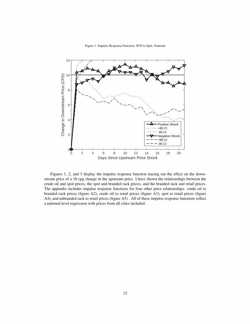
Figure 1: Impulse Response Function: WTI to Spot, National

Days Since Upstream Price Shock0 2 4 6 8 10 12 14 16 18 20

Cha

nge

in D

owns

trea

m P

rice

(CP

G)

0

2

4

6

8

10

12

Positive Shock+95 CI-95 CINegative Shock+95 CI-95 CI

Figures 1, 2, and 3 display the impulse response function tracing out the effect on the down-stream price of a 10 cpg change in the upstream price. I have shown the relationships between thecrude oil and spot prices, the spot and branded rack prices, and the branded rack and retail prices.The appendix includes impulse response functions for four other price relationships: crude oil tobranded rack prices (figure A2), crude oil to retail prices (figure A3), spot to retail prices (figureA4), and unbranded rack to retail prices (figure A5) . All of these impulse response functions reflecta national-level regression with prices from all cities included.

12

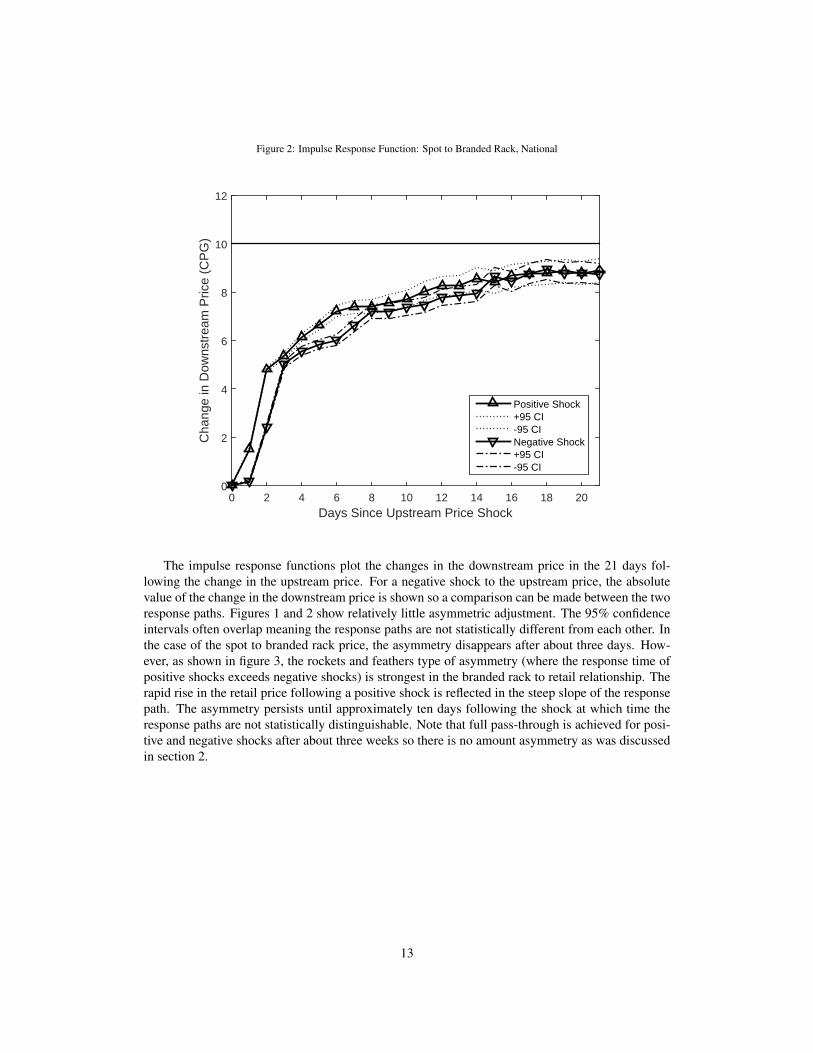
Figure 2: Impulse Response Function: Spot to Branded Rack, National

Days Since Upstream Price Shock0 2 4 6 8 10 12 14 16 18 20

Cha

nge

in D

owns

trea

m P

rice

(CP

G)

0

2

4

6

8

10

12

Positive Shock+95 CI-95 CINegative Shock+95 CI-95 CI

The impulse response functions plot the changes in the downstream price in the 21 days fol-lowing the change in the upstream price. For a negative shock to the upstream price, the absolutevalue of the change in the downstream price is shown so a comparison can be made between the tworesponse paths. Figures 1 and 2 show relatively little asymmetric adjustment. The 95% confidenceintervals often overlap meaning the response paths are not statistically different from each other. Inthe case of the spot to branded rack price, the asymmetry disappears after about three days. How-ever, as shown in figure 3, the rockets and feathers type of asymmetry (where the response time ofpositive shocks exceeds negative shocks) is strongest in the branded rack to retail relationship. Therapid rise in the retail price following a positive shock is reflected in the steep slope of the responsepath. The asymmetry persists until approximately ten days following the shock at which time theresponse paths are not statistically distinguishable. Note that full pass-through is achieved for posi-tive and negative shocks after about three weeks so there is no amount asymmetry as was discussedin section 2.

13

Figure 3: Impulse Response Function: Branded Rack to Retail Prices, National

Days Since Upstream Price Shock0 2 4 6 8 10 12 14 16 18 20

Cha

nge

in D

owns

trea

m P

rice

(CP

G)

0

2

4

6

8

10

12

Positive Shock+95 CI-95 CINegative Shock+95 CI-95 CI

A convenient way to quantify the asymmetry is to calculate the following:

Impact =∫

t∈T ∗∆+P(t)−|∆−P(t)|dt, (8)

where T ∗ defines any time period where the response paths are significantly different from eachother. ∆+P(t) and |∆−P(t)| are simply the (absolute) changes in downstream prices at time t fol-lowing positive and negative shocks respectively. In figure 3, the estimate of impact simplifies tocalculating the average price following a positive shock and subtracting the average price followinga negative shock where the average is taken over the first ten periods.

14

Figure 4: Impact Estimates

Impact estimates for each price series are shown in figure 4. The largest impact of 2.27 cpg isfor the branded rack to retail relationship. Other relationships show a positive and significant im-pact between 1 and 1.5 cpg.27 The real-world interpretation of this result is as follows. Considertwo 3-week periods, one following a one-time rack price increase from 200 cpg to 210 cpg and onefollowing a one-time rack price decrease from 210 cpg to 200 cpg. Assume consumers randomlypurchased retail gasoline over the course of each period. With symmetric pass-through, consumerswould on average pay the same amount for retail gasoline over both periods. However, with asym-metric pass-through, consumers purchasing retail gasoline following a rack price increase will pay2.27 cpg more than consumers purchasing retail gasoline following a decrease in the rack price.

Bacon (1991) found a similar asymmetry in rack to retail prices, while Bachmeier and Griffin(2003) find no evidence of asymmetry in the crude oil to gasoline spot price transmission, consistentwith my results. BCG (1997) do not find any significant asymmetry in the gasoline spot to rackrelationship, but they do find significant asymmetry in the crude to gasoline spot and the rack toretail relationships. Since BCG relies on bi-weekly data, I have also run my specifications usingonly prices from every other week and my impact results are larger though the estimates are basedon different cities over a different period of time.28

27The confidence interval on the WTI to Gulf gasoline spot relationship is larger than the others due to fewer observations.Other specifications estimate the average impact over multiple retail and wholesale market areas.

28The rack (wholesale) to retail impact estimate in BCG is 1 cpg while I estimate the impact to be 1.57 cpg. The estimatein BCG is based on 164 bi-weekly observations, while I am fortunate to have over 130 thousand daily observations.

15

4.2. Individual City Results

The evidence of asymmetry found in the previous section is mostly confirmed by regressionsrun at the individual city level. I focus only the branded rack to retail price relationships analyzedin the last section. Table 5 shows the estimates and t-statistics for the contemporaneous coefficientson the positive and negative rack changes. The positive and significant difference between each setof coefficients shows evidence of rockets and feathers asymmetry in every city in the sample.

Table 5: Difference in First Coefficients on Lagged Upstream Price

β+1 t-stat β

−1 t-stat β

+1 −β

−1 t-stat

Atlanta 0.21*** 30.94 0.04*** 6.15 0.17*** 17.63Boston 0.16*** 33.24 0.05*** 10.92 0.11*** 16.40Chicago 0.22*** 31.84 0.07*** 11.02 0.15*** 14.97Cleveland 0.41*** 27.61 0.13*** 8.73 0.29*** 13.86Dallas 0.17*** 30.79 0.07*** 13.03 0.10*** 12.90Denver 0.12*** 23.78 0.03*** 6.79 0.09*** 12.23Detroit 0.42*** 48.75 0.16*** 19.11 0.26*** 21.53Washington DC 0.14*** 12.76 0.03*** 2.75 0.11*** 7.18Washington MD 0.14*** 29.16 0.04*** 9.05 0.10*** 14.50Washington VA 0.13*** 27.25 0.05*** 9.89 0.08*** 12.48Washington WV 0.10*** 9.76 0.06*** 6.05 0.04*** 2.65Houston 0.16*** 42.73 0.05*** 13.00 0.12*** 21.57Los Angeles 0.30*** 39.24 0.06*** 8.24 0.24*** 22.78Louisville IN 0.27*** 15.42 0.07*** 4.40 0.20*** 8.17Louisville KY 0.43*** 16.60 0.12*** 4.93 0.31*** 8.57Miami 0.16*** 37.19 0.04*** 9.68 0.12*** 20.17Minneapolis St Paul MN 0.43*** 26.51 0.12*** 7.31 0.32*** 14.00Minneapolis St Paul WI 0.13*** 14.73 0.06*** 6.63 0.07*** 5.98New Orleans 0.17*** 30.72 0.06*** 11.77 0.11*** 14.26Newark 0.14*** 24.11 0.06*** 10.96 0.08*** 10.23New York 0.09*** 16.61 0.05*** 9.66 0.04*** 5.61Phoenix 0.20*** 18.65 0.06*** 5.93 0.13*** 8.78Salt Lake City 0.16*** 12.84 0.08*** 6.58 0.08*** 4.73San Francisco 0.25*** 27.70 0.08*** 8.49 0.17*** 13.64Seattle 0.21*** 32.28 0.06*** 9.38 0.15*** 16.65St Louis IL 0.24*** 18.20 0.12*** 8.84 0.12*** 6.57St Louis MO 0.37*** 16.94 0.15*** 7.05 0.21*** 6.97National Specification 0.23*** 100.00 0.08*** 34.13 0.15*** 47.83

Estimates from the branded rack to retail specification, by city. Estimates of the firstdifference in positive and negative rack price coefficients. Positive and significant differ-ences are evidence of rockets and feathers. Significant at the 1% (***) level.

16

Figure 5: Impact of Asymmetric Adjustment, By City, Branded Rack to Retail

While I find evidence of asymmetric pass-through from branded rack to retail prices in everycity, the overall impact of the asymmetry can only be achieved by estimating the impulse responsefunction and calculating the impact as shown in equation 8. These results are reported in figure 5.Salt Lake City features the largest asymmetry with an impact of about 4.5 cpg (even though thelargest differential in the β1 estimates was in Minneapolis-MN). Other cities, such as, Louisville-IN,Cleveland, and Minneapolis-MN also show relatively more asymmetry, while Minneapolis-WI, St.Louis-IL, and New York have the least asymmetry.29 I also calculate the speed of pass-through bycomparing the slopes of the impulse response functions over the first three periods following thecost shock. The speed of pass-through is between three and four times faster when rack prices risethan when they fall.

Interestingly, while three of the retail areas that straddle state lines show similar levels of asym-metry on both sides of the line (Louisville, St. Louis, and Washington), Minneapolis shows signif-icantly more asymmetry west of the Mississippi and less to the east. One potential explanation isdue to population density: Minneapolis, WI is much more rural than Minneapolis, MN. The otherstate-straddling areas are more urban on both sides of the border.30

29The data feature several periods when the observed retail price is less than the rack price. This may result from short-term shortages at the wholesale level. This happens sporadically and primarily in four areas (Louisville-KY, Phoenix-AZ,StLouis-IL, and StLouis-MO). I have run the national specification and individual city models excluding these periods andthe estimates of asymmetry are essentially unchanged.

30The population density in the Minnesota counties around Minneapolis is over 6 times the population density in the nearbyWisconsin counties based on the 2010 census. Washington-WV also has a population density less than half that of the otherWashington area metro areas, and it also shows relatively less asymmetric adjustment.

17

Finally, note that the national-specification impact estimate (2.27 cpg) is not a simple averageof the city-level estimates (3.28 cpg) because each impact is calculated as the difference in theimpulse response functions over days when they are statistically different. The number of days inthis calculation varies from city to city and for the national specification.

4.3. Time Aggregation

One of the major differences between the various studies in the extant literature is the frequencyof the data used. Many rely on less frequent, bi-weekly or monthly data simply because it it morewidely available. In this section, I consider the effect of using daily versus weekly data on thelikelihood of finding evidence of pass-through asymmetry.

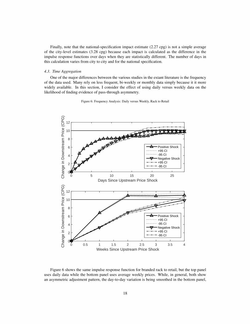
Figure 6: Frequency Analysis: Daily versus Weekly, Rack to Retail

Days Since Upstream Price Shock0 5 10 15 20 25C

hang

e in

Dow

nstr

eam

Pric

e (C

PG

)

0

2

4

6

8

10

12

Positive Shock+95 CI-95 CINegative Shock+95 CI-95 CI

Weeks Since Upstream Price Shock0 0.5 1 1.5 2 2.5 3 3.5 4C

hang

e in

Dow

nstr

eam

Pric

e (C

PG

)

0

2

4

6

8

10

12

Positive Shock+95 CI-95 CINegative Shock+95 CI-95 CI

Figure 6 shows the same impulse response function for branded rack to retail, but the top paneluses daily data while the bottom panel uses average weekly prices. While, in general, both showan asymmetric adjustment pattern, the day-to-day variation is being smoothed in the bottom panel,

18

which masks the pass-through dynamics between the two price series. The results are very similarwhen using weekly prices based on a specific day of each week instead of weekly averages. Theimpact of asymmetry is 2.80 cpg using average weekly prices and 2.77 cpg using once-per-weekprices.31

The weekly impact estimate is significantly higher than the impact based on daily price changes(2.27 cpg). Comparing the impulse response functions, it is clear that using daily data, retail pricesare predicted to rise slower following a positive cost shock and fall faster following a negative costshock compared with weekly data.32 Both of these effects cause the impact estimate to be largerbased on the weekly data, but complete pass-through is achieved for both positive and negativeshocks by about four weeks using either frequency of data.

4.4. Branded versus Unbranded

Branded wholesale gasoline is generally a few cents more expensive than unbranded gasolinegiven the former has proprietary additives (and a brand-name premium) included. However, at times,the unbranded price will exceed the branded price, and this occurs especially following negativesupply shocks. As shown in figure 7, the asymmetry for branded gasoline is significantly higherthan for unbranded gasoline in about one-half of the retail market areas.33

31The once-per-week specification generally uses the price on Wednesday of each week, though when that price is missing,the Tuesday or Thursday price is selected.

32Based on daily (weekly) data, complete pass-through is achieved in 28 (12) days following positive shocks and 17 (25)days following negative shocks.

33The impulse response function for the unbranded rack to retail relationship is shown in figure A5. The impact estimate forthe unbranded rack to retail national specification is 1.12 cpg, about half that found in the branded rack to retail relationship(2.27 cpg).

19

Figure 7: Impact of Asymmetric Adjustment, By City, Branded versus Unbranded

Impa

ct (

CP

G)

0

1

2

3

4

5

6

7

8

Sal

t Lak

e C

ity

Loui

svill

e IN

C

leve

land

M

inne

apol

is S

t Pau

l MN

Los

Ang

eles

Loui

svill

e K

Y

Den

ver

W

ashi

ngto

n D

C

Sea

ttle

A

tlant

a

Was

hing

ton

MD

P

hoen

ix

Was

hing

ton

VA

S

an F

ranc

isco

D

alla

s

Bos

ton

H

oust

on

Mia

mi

S

t Lou

is M

O

C

hica

go

Was

hing

ton

WV

N

ewar

k

New

Orle

ans

Det

roit

N

atio

nal S

peci

ficat

ion

Min

neap

olis

St P

aul W

IS

t Lou

is IL

New

Yor

k

BrandedUnbranded

Therefore, while the unbranded price “rockets up” more quickly than the branded price followinga supply shock, the unbranded price also retreats back to equilibrium levels at a faster pace thanthe branded price. In some cities, such as, Seattle, Cleveland, and Los Angeles, the difference inasymmetry is very large with branded prices being more than twice as asymmetric compared withunbranded prices. The result that unbranded gasoline prices exhibit less asymmetry is consistentwith the literature that claims heterogeneous consumer search costs are the cause of asymmetricadjustment (e.g., Lewis (2011)). Consumers who buy branded gasoline are likely more loyal to asingle brand, while unbranded buyers are more likely to shop around for the best price. A negativecost shock would be passed on more quickly to unbranded prices than to branded prices, reducingthe asymmetry in the unbranded price relationship.

4.5. Differences Over TimeWhile the previous results display the differences in asymmetry in different price relationships

and cities for a single permanent change in the upstream price, the actual impact of the rockets andfeathers phenomenon depends on how the variability of the price series being analyzed changesthrough time. More data are required to identify how the pass-through relationship has changedover time (i.e. the coefficients in equation 1), so in this section I quantify the amount of asymmetryin each year of the sample using the same set of estimated coefficients. The extreme cases, whenprices always rise or always fall, result in complete rockets behavior or complete feathers behaviorrespectively. If prices are fairly stable or upstream prices generally rise, the impact of asymmetricpass-through will be small, while the feathering effect will be large if prices generally fall duringthe sample period.

20

To quantify the impact of asymmetric pass-through over time, I use the actual upstream (rack)price and estimate the downstream (retail) price under two regimes. First, I calculate the predictedprice using the estimates of my model (i.e., those that reflect the asymmetric pass-through or therockets and feathers regime). Assuming the model fits the data well, the predicted prices will bevery close to the actual retail prices. In the second regime, I estimate the retail prices if they respondto negative shocks in the rack price at the same rate that they respond to positive shocks. In practice,this means simply replacing the β

−1i coefficients with the β

+1i coefficients for i = 1, . . . ,L1. I call

this the rockets and rockets regime (abbreviated RR in the figures). I can then estimate the averagedownstream price under each regime and determine how much higher prices are under rockets andfeathers as compared with rockets and rockets.

Figure 8: Simulation: Rockets and Feathers vs Rockets and Rockets, 2013

MonthJan Feb Mar Apr May Jun Jul Aug Sep Oct Nov Dec Jan

Pric

e (C

PG

)

240

250

260

270

280

290

300

310

320

330

RackSimulated Retail (RF)Simulated Retail (RR)

Simulation based on the national specification for branded rack and retail prices, January-December 2013. The mean RFprice was 301.72 and the mean RR price was 298.37, a difference of 3.35 cpg.

Figure 8 shows the results of the simulation for 2013. I run the national model over the entiresample period from 2000 to 2013 and then simulate prices under the two regimes during 2013 alone.The red dashed line shows the predicted retail price under the rockets and feathers regime and theblue dashed line shows the predicted prices under the rockets and rockets regime. The graph showsthat the retail prices increase at approximately the same rate when the rack price is increasing, whilethe blue line falls back much slower than the red line. Overall the average retail price is 301.72 cpgunder rockets and feathers and 298.37 cpg under rockets and rockets, a difference of 3.35 cpg. Thereason this difference is larger than the impact estimate in section 4.1 is that rack prices were volatilein 2013 with frequent periods of slowly falling retail prices.

21

Figure 9: Simulation: Rockets and Feathers vs Rockets and Rockets, By Year

Figure 9 shows the difference in the average retail price under the two regimes for each yearfrom 2000 to 2013. Again, these results are all based on the same set of coefficients (i.e., the modelrun on all cities/years and not separate models for each year). The year-by-year variation is due tothe differences in the volatility of rack prices in each year. The spike in 2008 is due to a long declinein rack prices in the second half of the year, which means there is significant feathering of retailprices and the impact is large. All else equal, based on the average across all years, retail priceswould be about 2.45 cpg lower if retail prices fell as quickly as they rose.34

It is important to note that the simulated prices under the rockets and rockets regime may not bethe outcome one would expect under any model of competition. The simulation is simply a coun-terfactual experiment to determine how much higher are prices when they feather down instead ofrocket down. If symmetric pass-through or a constant markup over the wholesale price was in someway required, retail station owners may respond by changing their pricing strategy so the averagemarkup is the same under asymmetric or symmetric pass-through. In other words, by requiringsymmetric pass-through, it is not clear that consumers would necessarily benefit from lower averageretail prices. In fact, under the rockets and rockets counterfactual, the average markup drops by 2.45cpg, which may cause firms to exit. Thus the welfare consequences of eliminating asymmetric pass-through are ambiguous and the counterfactual serves as an experiment to estimate the magnitude ofthe impact that feathering has on retail prices, all else equal.

34The 95% confidence interval for the 14-year average impact is (1.18 cpg, 3.72 cpg).

22

4.6. Formal Tests of Asymmetry

In order to formally test for asymmetry, I report F-statistics for the pattern asymmetry in equation5. I test the following hypothesis:

H0 : β+1i = β

−1i ∀ i

H1 : β+1i 6= β

−1i for some i.

Note this is a two-sided test, so includes the possibility that the asymmetry is both the rockets andfeathers type and the opposite. To implement the test, I save the residual sum of squares, RSSu, fromthe full (unrestricted) model where the coefficients are allowed to vary separately for positive andnegative shocks. I then estimate a symmetric (restricted) model, with only one set of β1i coefficientsand save RSSr. Note that minimizing the BIC separately for each model would mean that a differentnumber of lags is included in each.35 Therefore, I again restrict the number of lags to be 21 daysin both regressions so the only difference between the models is the restriction on the parameters.36

Results are reported in table 6.

35See Ye, et. al. (2005) for a discussion of this issue.36Formally, the test statistic is of the usual form, F =

(RSSr−RSSu)/(Ku−Kr)

RSSu/(N−Ku), where Ku and Kr are the number of

parameters to be estimated in the unrestricted and restricted models respectively.

23

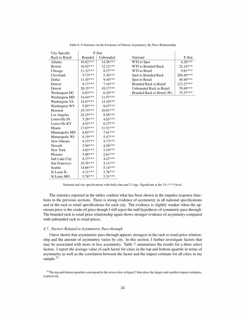
Table 6: F-Statistics on the Existence of Pattern Asymmetry, By Price Relationship

City-Specific F-StatRack to Retail Branded UnbrandedAtlanta 16.82*** 14.56***Boston 16.92*** 12.12***Chicago 11.32*** 8.27***Cleveland 9.73*** 5.30***Dallas 11.45*** 9.44***Denver 9.17*** 7.16***Detroit 20.35*** 10.17***Washington DC 6.83*** 6.29***Washington MD 14.44*** 11.97***Washington VA 14.87*** 14.10***Washington WV 5.05*** 8.67***Houston 19.74*** 10.01***Los Angeles 24.25*** 9.56***Louisville IN 5.28*** 4.63***Louisville KY 4.92*** 6.27***Miami 17.03*** 11.51***Minneapolis MN 8.65*** 7.61***Minneapolis WI 6.19*** 5.47***New Orleans 9.15*** 4.73***Newark 5.94*** 4.26***New York 4.65*** 3.19***Phoenix 5.88*** 2.61***Salt Lake City 8.37*** 4.47***San Francisco 10.76*** 4.11***Seattle 14.66*** 5.14***St Louis IL 4.31*** 3.76***St Louis MO 5.78*** 5.31***

National F-StatWTI to Spot 6.26***WTI to Branded Rack 22.14***WTI to Retail 9.81***Spot to Branded Rack 204.49***Spot to Retail 40.40***Branded Rack to Retail 123.27***Unbranded Rack to Retail 70.49***Branded Rack to Retail (W) 75.37***

National and city specifications with daily data and 21 lags. Significant at the 1% (***) level.

The statistics reported in the tables confirm what has been shown in the impulse response func-tions in the previous sections. There is strong evidence of asymmetry in all national specificationsand in the rack to retail specifications for each city. The evidence is slightly weaker when the up-stream price is the crude oil price though I still reject the null hypothesis of symmetric pass-through.The branded rack to retail price relationship again shows stronger evidence of asymmetry comparedwith unbranded rack to retail prices.

4.7. Factors Related to Asymmetric Pass-through

I have shown that asymmetric pass-through appears strongest in the rack to retail price relation-ship and the amount of asymmetry varies by city. In this section, I further investigate factors thatmay be associated with more or less asymmetry. Table 7 summarizes the results for a three selectfactors. I report the average value of each factor for cities in the top and bottom quartile in terms ofasymmetry as well as the correlation between the factor and the impact estimate for all cities in mysample.37

37The top and bottom quartiles correspond to the seven cities in figure 5 that show the largest and smallest impact estimates,respectively.

24

Table 7: Factors related to asymmetric pass-through

FactorCycling Speed Concentration

Top Quartile Asymmetric -0.52 9.79 1,620Bottom Quartile Asymmetric -0.17 13.29 1,419Correlation(Asymmetry, Factor) -0.26 -0.23 0.18

Notes: Cycling is measured by the median first difference of retail pricechanges. Cycling is more prevalent in cities with larger (negative) es-timates. Speed is calculated as the number of days to reach 90% pass-through for positive and negative wholesale cost shocks. Concentrationis the brand-level HHI based on the total revenue sales by gas stationsin each city.

For each city in the sample, I estimate a statistic on price cycling measured as the median firstdifference of daily changes in the retail price. Larger (absolute) values of this statistic are evidenceof price cycling: if increases in price are relatively large and occur quickly while decreases tend tobe small and last for many periods, the median first difference will be more negative. Asymmetryis negatively associated with this statistic, which implies that cities that show more asymmetricadjustment also are more likely to cycle.38 Asymmetry is also negatively related to the speed ofpass-through, measured as the number of days to pass-through 90% of a cost shock (positive ornegative). In fact, cycling and pass-through speed are strongly correlated (ρ = 0.88), consistentwith the findings in Lewis and Noel (2011).

Finally, I calculate a brand-level concentration index for cities in my sample based on data fromNew Image Marketing Research Corporation. I calculate the Herfindahl-Hirschman Index (HHI) foreach city based on the total dollar sales at all stations in a city around the first year in my sample.39

Concentration is positively correlated with asymmetric pass-through, consistent with the findingsin Deltas (2008) and Verlinda (2008). The HHI is about 14% higher for cities in the top quartileof asymmetry relative to the bottom quartile. Other factors, such as gasoline tax levels, medianhousehold income, and percent of sales by channel (e.g., rack versus DTW), are uncorrelated withthe amount of asymmetric pass-through observed in each city.

5. Conclusion

The purpose of this study was to understand why so many researchers have studied asymmetricpass-through in the gasoline industry and have come to varying conclusions about its existenceand causes. Many of the discrepancies can be explained by variations in the data and the modelspecification. I find that pass-through asymmetries do exist in all price relationships from the priceof crude oil, to spot, rack and retail gasoline prices. Pass-through asymmetry in the branded rackto retail price relationship is shown to be larger than its unbranded counterpart, consistent with theexplanation that consumer search costs drive asymmetric pass-through. Averaging daily data toobtain a weekly price series leads to a larger estimate of asymmetry as retail prices are predicted toincrease faster following a cost increase and fall slower following a cost decrease.

38Minneapolis, MN is in the top quartile of cities and shows evidence of cycling (median first difference = -0.77) whileMinneapolis, WI show relatively less asymmetry and little evidence of cycling (median first difference = -0.08).

39I have data on 22 of the 27 cities in the sample for one of the years between 1998 and 2001. Using total sales by all gasstations that sell under each brand name, I calculate HHI = ∑i s2

i , where si is the share of brand i.

25

Estimating the model separately for each city in the sample shows that some cities experiencemore asymmetric pass-through than others, but in every city, the speed of pass-through is betweenthree and four times faster when rack prices rise than when they fall. I find that asymmetry inpass-through rates is positively correlated with both the degree of price cycling and overall speedof pass-through in a city. I also find evidence consistent with explanations of asymmetry based onmarket power as the amount of asymmetry is positively associated with retail concentration.

The magnitude of the impact of asymmetric pass-through is economically significant. I find thatretail prices would be about 3.35 cpg lower in 2013 if retail price fell as quickly as they rose. This isabout 1% of the retail gasoline price, though it is 15.2% of the average markup of retail over brandedrack prices seen in the data.40 While significant, it is important to keep these findings within thescope of the model, as estimating the welfare implications of eliminating asymmetric pass-throughwould require a fully structural model of wholesale and retail gasoline pricing. Determining thegeneral equilibrium effects is an appropriate extension to this line of research and may provideimportant insights into the effects of asymmetric pass-through in gasoline prices as well as othermarkets.

40The average retail price across all cities in 2013 was 305 cpg and the average rack price was 284 cpg.

26

References

Bachmeier, Lance and James Griffin (2003). “New Evidence on Asymmetric Gasoline Price Re-sponses.” The Review of Economics and Statistics 85(3): 772-776.

Bacon, Robert W. (1991). “Rockets and Feathers: The Asymmetric Speed of Adjustment of UKRetail Gasoline Prices to Cost Changes.” Energy Economics 13(3): 211-218.

Bonnet, C. and S. B. Villas-Boas (2013). “An Analysis of Asymmetric Consumer Price Responsesand Asymmetric Cost Pass-Through in the French Coffee Market.” TRANSFOP Working paper N.10.

Borenstein, S., C. A. Cameron and R. Gilbert (1997). “Do Gasoline Prices Respond Asymmetricallyto Crude Oil Price Changes?” Quarterly Journal of Economics 112(1): 305-339.

Borenstein, S. (1991). “Selling Costs and Switching Costs: Explaining Retail Gasoline Margins.”The RAND Journal of Economics 22(3): 354-369.

Borenstein, S., Andrea Shepard (1996). “Dynamic Pricing in Retail Gasoline Markets.” The RANDJournal of Economics 27(3): 429-451.

Bulow, Jeremy and Paul Pfleiderer (1983). “A Note on the Effect of Cost Changes on Prices.” Journalof Political Economy 91(1): 182-185.

Deltas, George (2008). “Retail Gasoline Price Dynamics and Local Market Power.” The Journal ofIndustrial Economics 56(3): 613-628.

Eckert, Andrew (2002). “Retail Price Cycles and Response Asymmetry.” Canadian Journal of Eco-nomics 35(1): 52-77.

Energy Information Administration, U.S. Department of Energy (2007). “Refinery Outages: De-scription and Potential Impact on Petroleum Product Prices.”

Energy Information Administration, U.S. Department of Energy (2008). “A Primer on Gaso-line Prices.” Online: http://www.eia.gov/energyexplained/print.cfm?page=gasoline_factors_affecting_prices [Downloaded: 1/13/2015].

Engle R. and C.W.J. Granger (1987). “Co-Integration and Error Correction: Representation, Esti-mation, and Testing.” Econometrica 55(2): 251-276.

Espey, Molly (1996). “Explaining Variation in Elasticity of Gasoline Demand in the United States:A Meta Analysis.” The Energy Journal 17(3): 49-60.

The Federal Trade Commission (2006). “Investigation of Gasoline Price Manipulation and Post-Katrina Gasoline Price Increases.” Available at http://www.ftc.gov/reports/federal-

trade-commission-investigation-gasoline-price-manipulation-post-katrina-

gasoline.

The Federal Trade Commission (2005). “Gasoline Price Changes: The Dynamics of Sup-ply, Demand and Competition.” Available at http://www.ftc.gov/reports/gasprices05/050705gaspricesrpt.pdf.

Gautier, E. and R. Le Saout (2012). “The dynamics of gasoline prices: evidence from daily Frenchmicro data.” Banque de France Working Paper No. 375.

27

Godby, R, A.M. Lintner, T. Stengos, and B. Wandschneider (2000). “Testing for Asymmetric Pricingin the Canadian Retail Gasoline Market.” Energy Economics 22(3): 349-368.

Goldberg, Pinelopi K. and Rebecca Hellerstein (2008). “A Structural Approach to Explaining In-complete Exchange-Rate Pass-Through and Pricing-to-Market.” The American Economic Review98(2): 423-429.

Goodwin, Barry, and Matthew Holt (1999). “Price Transmission and Asymmetric Adjustment in theU.S. Beef Sector.” American Journal of Agricultural Economics 81(3): 630-637.

The Government Accountability Office (2006). “Energy Markets: Factors Contributing to HigherGasoline Prices.” GAO-06-412T.

Gron, Anne, and Deborah Swenson (2000). “Cost Pass-Through in the U.S. Automobile Market.”The Review of Economics and Statistics 82(2): 316-324.

Hastings, Justine, Jennifer Brown, Erin Mansur, and Sofia Villas-Boas (2008). “Reformulating Com-petition? Gasoline Content Regulation and Wholesale Gasoline Prices.” Journal of EnvironmentalEconomics and Management 55(1): 1-19.

Hosken, Daniel, Robert McMillan and Christopher Taylor (2008). “Retail Gasoline Pricing: WhatDo We Know?” International Journal of Industrial Organization 26(6): 1425-1436.

Kim, Donghun and Ronald Cotterill (2008). “Cost Pass-Through in Differentiated Product Markets:The Case of U.S. Processed Cheese.” The Journal of Industrial Economics 56(1): 32-48.

Knittel, Christopher, Jonathan E. Hughes, and Daniel Sperling (2008). “Evidence of a Shift in theShort-Run Price Elasticity of Gasoline Demand.” The Energy Journal 29(1): 113-134.

Lewis, Matthew (2011). “Asymmetric Price Adjustment and Consumer Search: an Examination ofRetail Gasoline Market.” Journal of Economics and Management Strategy 20(2): 409-449.

Lewis, Matthew and Howard P. Marvel (2011). “When Do Consumers Search?” Journal of Indus-trial Economics 59(3): 457-483.

Lewis, Matthew, and Michael Noel (2011). “The Speed of Gasoline Price Response in Markets withand without Edgeworth Cycles.” The Review of Economic Studies 93(2): 672-682.

Lewis, Matthew (2009). “Temporary Wholesale Gasoline Price Spikes have Long Lasting RetailEffects: The Aftermath of Hurricane Rita.” Journal of Law and Economics 52(3), 581-605.

Lewis, Matthew (2012). “Price Leadership and Coordination in Retail Gasoline Markets with PriceCycles.” International Journal of Industrial Organization 30(4): 342-351.

Lidderdale, Tancred (1999). “Environmental Regulations and Changes in Petroleum Refining Op-erations.” United States Energy Information Administration Report. Online: http://www.eia.

doe.gov/emeu/steo/pub/special/enviro.html [Downloaded: 1/13/2015].

MacKinnon, James (2010). “Critical Values for Cointegration Tests.” Queen’s Economics Depart-ment Working Paper No. 1227.

Muller, Georg and Sourav Ray (2007). “Asymmetric Price Adjustment: Evidence from WeeklyProduct-Level Scanner Price Data.” Managerial and Decision Economics 28(7): 723-736.

28

Noel, Michael D. (2007). “Edgeworth Price Cycles, Cost-Based Pricing, and Sticky Pricing in RetailGasoline Markets.” Review of Economics and Statistics 89(2): 324-334.

Noel, Michael D. (2009). “Do Gasoline Prices Respond Asymmetrically to Cost Shocks? The Effectof Edgeworth Cycles.” RAND Journal of Economics 40(3): 582-595.

Peterson, D. J. and Sergej Mahnovski (2003). New Forces at Work in Refining: Industry Views ofCritical Business and Operations Trends. Santa Monica, CA: RAND Corporation.

The United States Senate (2002). “Gas Prices: How are they Really Set?” Online: http://www.hsgac.senate.gov/download/report_gas-prices-how-are-they-really-set [Down-loaded 1/13-2015].

Tappata, Mariano (2009). “Rockets and Feathers: Understanding Asymmetric Pricing.” The RANDJournal of Economics 40(4): 673-687.

Ten Kate, Adriaan and Gunnar Niels (2005). “To What Extent are Cost Savings Passed on to Con-sumers? An Oligopoly Approach.” European Journal of Law and Economics 20(3): 323-337.

Verlinda, Jeremy (2008). “Do Rockets Rise Faster and Feathers Fall Slower in an Atmosphere ofLocal Market Power? Evidence from the Retail Gasoline Market” Journal of Industrial Economics56(3): 581-612.

Ye, Michael, John Zyren, Joanne Shore, and Michael Burdette (2005). “Regional Comparisons,Spatial Aggregation, and Asymmetry of Price Pass-Through in U.S. Gasoline Markets.” AtlanticEconomic Journal 33(2): 179-192.

Yang, H. and L. Ye L. (2008). “Search with Learning: Understanding Asymmetric Price Adjust-ments.” The RAND Journal of Economics 39(2): 547-564.

Zimmerman, Paul R., John M. Yun, and Christopher T. Taylor (2013). “Edgeworth Price Cycles inGasoline: Evidence from the United States.” Review of Industrial Organization 42(3): 297-320.

29

Appendix A. Additional Figures and Tables

Figure A1: St. Louis Retail Market Areas

Figure A2: Impulse Response Function: WTI to Branded Rack, National

Days Since Upstream Price Shock0 2 4 6 8 10 12 14 16 18 20

Cha

nge

in D

owns

trea

m P

rice

(CP

G)

0

2

4

6

8

10

12

Positive Shock+95 CI-95 CINegative Shock+95 CI-95 CI

30

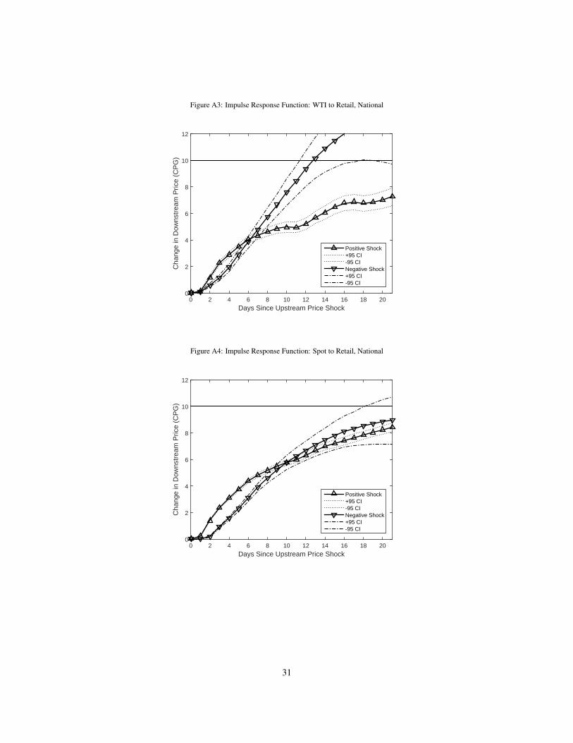
Figure A3: Impulse Response Function: WTI to Retail, National

Days Since Upstream Price Shock0 2 4 6 8 10 12 14 16 18 20

Cha

nge

in D

owns

trea

m P

rice

(CP

G)

0

2

4

6

8

10

12

Positive Shock+95 CI-95 CINegative Shock+95 CI-95 CI

Figure A4: Impulse Response Function: Spot to Retail, National

Days Since Upstream Price Shock0 2 4 6 8 10 12 14 16 18 20

Cha

nge

in D

owns

trea

m P

rice

(CP

G)

0

2

4

6

8

10

12

Positive Shock+95 CI-95 CINegative Shock+95 CI-95 CI

31

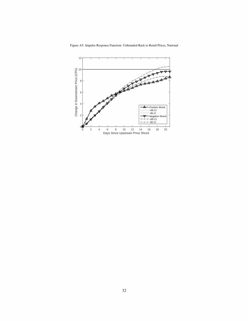
Figure A5: Impulse Response Function: Unbranded Rack to Retail Prices, National

Days Since Upstream Price Shock0 2 4 6 8 10 12 14 16 18 20

Cha

nge

in D

owns

trea

m P

rice

(CP

G)

0

2

4

6

8

10

12

Positive Shock+95 CI-95 CINegative Shock+95 CI-95 CI

32