gas-leak localization using distributed ultrasonic sensorsbic/papers/spie.pdf · gas-leak...

ULTRASONIC SOURCE

LIILII ((

MICROPHONES

Gas-Leak Localization Using Distributed Ultrasonic Sensors

Javid Huseynova,b, Shankar Baligab, Michael Dillencourta, Lubomir Bica, Nader Bagherzadeha

aBren School of Information and Computer Science, University of California, Irvine, CA 92697bGeneral Monitors Transnational, 26776 Simpatica Circle, Lake Forest, CA 92630

ABSTRACT

We propose an ultrasonic gas leak localization system based on a distributed network of sensors. The systemdeploys highly sensitive miniature Micro-Electro-Mechanical Systems (MEMS) microphones and uses a suite ofenergy-decay (ED) and time-delay of arrival (TDOA) algorithms for localizing a source of a gas leak. Statisticaltools such as the maximum likelihood (ML) and the least squares (LS) estimators are used for approximatingthe source location when closed-form solutions fail in the presence of ambient background nuisance and inherentelectronic noise. The proposed localization algorithms were implemented and tested using a Java-based simulationplatform connected to four or more distributed MEMS microphones observing a broadband nitrogen leak from anorifice. The performance of centralized and decentralized algorithms under ED and TDOA schemes is analyzedand compared in terms of communication overhead and accuracy in presence of additive white Gaussian noise(AWGN).

Keywords: ultrasonic source localization, MEMS microphone, maximum likelihood estimator, distributed al-gorithms, ultrasonic gas detection, sensor networks

1. INTRODUCTION

The reliable detection and localization of gas leaks is essential for ensuring safety and minimizing propertydamage. In industry, a primary approach for detecting gas leaks is based on the physical phenomenon ofabsorption of infrared energy by combustible gases such as methane, propane or ethane. Another approach is tomeasure the current generated by electrochemical cells or catalytic sensors to determine the amount of toxic orcombustible gas present. The third, and relatively new, method is detecting the acoustic wave emitted during agas leak. As opposed to the other detection methods described, acoustic gas detection cannot, as yet, measurethe amount or type of gas from an observed signal. However, and again unlike the other detection methods, theacoustic method can be developed to locate the source of a leak.

Figure 1. Distributed Source Localization

Use of ultrasonic frequencies, with the audio frequencies filtered out by an electrical bandpass filter, enablesthe measurement and localization of high-pressure gas leaks in an industrial environment while avoiding thedisturbance and nuisance at audio frequencies caused by reverberation, natural and man-made backgroundphenomena.1 To the best of our knowledge, the distributed localization of broadband gas-leak sources usingMEMS microphones in the ultrasonic frequency range has not been attempted before.

Primary author contact: [email protected], +1 949 581 4464

Smart Sensor Phenomena, Technology, Networks, and Systems 2009, edited byNorbert G. Meyendorf, Kara J. Peters, Wolfgang Ecke, Proc. of SPIE Vol. 7293,72930Z · © 2009 SPIE · CCC code: 0277-786X/09/$18 · doi: 10.1117/12.812058

Proc. of SPIE Vol. 7293 72930Z-1

The localization of an ultrasonic source is accomplished by using differences in ultrasonic signals received atspatially distributed microphones. There are two parameters that characterize these differences:2

• Interaural Level Difference (ILD), or the differential Energy Decay (ED)

• Interaural Time Difference (ITD), or the differential Time Delay of Arrival (TDOA)

The ILD, a difference in sound pressure level (SPL) measured at two different receivers (ears, microphones),is helpful for humans to localize a sound source. It is based on a simple physical property that a sound wavehas an amplitude which decays at a rate inversely proportional to the square of the distance from the sourceto measurement location.3 The ITD-based methods rely on phase differences in acoustic signals arriving atneighboring microphone sensors at the speed of sound.4

The localization of utrasonic gas leak sources is an inherently distributed target detection problem (Fig. 1).To localize a gas leak source in any signal frequency spectrum, individual sensors must first detect the presenceof a source from their local data. Then, a collaborative signal processing at the network level involves routinginformation through the network and fusing the data from different sensors to generate an estimate of the sourcelocation. Therefore, solutions proposed for ultrasonic localization are naturally applicable in the context ofwireless sensor networks (WSN).

Due to low-power nodes in WSN, efficient in-network data processing is a key factor for enabling WSN toextract useful information and to ensure efficiency and accuracy of detection.5–7 In terms of efficiency, radiocommunication is an energy consuming task and is identified in many deployments as the primary factor forsensor node’s battery exhaustion8 because emitting or receiving a packet is far more energy consuming thanlocal computations. Thus, the reduction of the amount of data transmissions and decentralized in-networkcomputation are the recognized design priorities for WSN algorithms.9

In this work, we propose and implement a suite of ED- and TDOA-based algorithms for localizing a broadbandultrasonic gas-leak source using distributed MEMS microphones. This research problem is novel from threeaspects: 1) the localization of gas leaks using ultrasonic broadband signals as an input; 2) the deployment ofMEMS microphones for a distributed ultrasonic localization, and 3) the application of Newton’s iterative methodas a decentralized implementation of ML acoustic localization.

2. BACKGROUND AND RELATED RESEARCH

Acoustic localization strategies can be traced back to the earliest radar and sonar localization systems.10 With thefirst application of microphone arrays to speech and speaker recognition in 1960s, beamforming techniques becamewidely popular for computing the direction of arrival (DOA) of sound.11–13 Yet the distributed applications ofacoustic localization in an industrial setup were not addressed until the development of low-cost microphonesand WSN.14

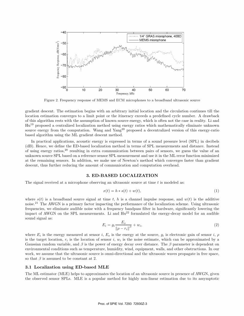
In recent years, low-cost MEMS microphones have been introduced to the consumer market. Such micro-phones surpass traditional Electret Condenser Microphones (ECM) in frequency response: many can be operatedup to 100 kHz in the utrasonic range, thereby opening up novel applications beyond the consumer audio market.MEMS microphones can also operate in a wide range of temperatures and consume less than a milliwatt of powerin operation, making them ideal for use in battery-powered wireless sensors. Figure 2 shows the ultrasonic per-formance of such a microphone out to 70 kHz, compared with an expensive 1

4 inch ultrasonic precision condenserpressure microphone (Type 40 BD) from G.R.A.S. Sound & Vibration.15 The experiments in this paper wereconducted using the omni-directional MSM2RM-S3035 MEMS microphone from Memstech Berhad.16

A number of ED- and TDOA-based algorithms have been developed for localizing sound sources in openspaces and reverberant room environments using distributed microphones. Yonak et al17 proposed a systemcombining optical and acoustic sensors for detecting and localizing gas leaks.

A decentralized incremental gradient algorithm for ED-based localization with known source energy wasproposed by Rabbat and Nowak.18 This algorithm relies on a priori knowledge of acoustic energy measured atthe source to estimate its location ρ by incrementally solving the error ML function at each sensor using steepest


-40

et 50C>

60a

70

80

900

1/4 GRAS microphone, 40BDMEMS microphone

10 20 30 40Frequency. kliz

50 60 70

Figure 2. Frequency response of MEMS and ECM microphones to a broadband ultrasonic source

gradient descent. The estimation begins with an arbitrary initial location and the circulation continues till thelocation estimation converges to a limit point or the itineracy exceeds a predefined cycle number. A drawbackof this algorithm rests with the assumption of known source energy, which is often not the case in reality. Li andHu19 proposed a centralized localization method using energy ratios which mathematically eliminate unknownsource energy from the computation. Wang and Yang20 proposed a decentralized version of this energy-ratiobased algorithm using the ML gradient descent method.

In practical applications, acoustic energy is expressed in terms of a sound pressure level (SPL) in decibels(dB). Hence, we define the ED-based localization method in terms of SPL measurements and distance. Insteadof using energy ratios,20 resulting in extra communication between pairs of sensors, we guess the value of anunknown source SPL based on a reference sensor SPL measurement and use it in the ML error function minimizedat the remaining sensors. In addition, we make use of Newton’s method which converges faster than gradientdescent, thus further reducing the amount of communication and computation overhead.

3. ED-BASED LOCALIZATION

The signal received at a microphone observing an ultrasonic source at time t is modeled as:

x(t) = h ∗ s(t) + w(t), (1)

where s(t) is a broadband source signal at time t, h is a channel impulse response, and w(t) is the additivenoise.21 The AWGN is a primary factor impacting the performance of the localization scheme. Using ultrasonicfrequencies, we eliminate audible noise with a frequency bandpass filter in hardware, significantly lowering theimpact of AWGN on the SPL measurements. Li and Hu22 formulated the energy-decay model for an audiblesound signal as:

Ei = giEs

‖ρ − ri‖β+ wi, (2)

where Ei is the energy measured at sensor i, Es is the energy at the source, gi is electronic gain of sensor i, ρis the target location, ri is the location of sensor i, wi is the noise estimate, which can be approximated by aGaussian random variable, and β is the power of energy decay over distance. The β parameter is dependent onenvironmental conditions such as temperature, humidity, wind, equipment, walls, and other obstructions. In ourwork, we assume that the ultrasonic source is omni-directional and the ultrasonic waves propagate in free space,so that β is assumed to be constant at 2.

3.1 Localization using ED-based MLE

The ML estimator (MLE) helps to approximates the location of an ultrasonic source in presence of AWGN, giventhe observed sensor SPLs. MLE is a popular method for highly non-linear estimation due to its assymptotic


efficiency in the limit T → ∞, where T denotes the observation interval.23 In order to apply the MLE, certainassumptions need to be made about the statistical behavior of the measurements, namely, that the measurementerror is modeled as Gaussian.21

In the ED-based localization, the MLE seeks to find a source position ρ(u, v) which maximizes the likelihoodof observing SPL values already measured at each sensor:

ρML = argmaxρ

Pr(L0, L1, . . . , Ln|ρ) (3)

Using the SPL definition and assuming β = 2, the sound energy degradation defined in (2) can be expressed as:

Li = LS − 20 logdi

dS+ εi, (4)

where dS is a unit distance from the source, di is a distance from the source to the microphone i, LS and Li arethe SPLs at the source and node i respectively, and εi is the additive dB noise, expressed as a logarithm of wi

from equation (2).

In order to solve the problem with unknown source SPL LS, we assume L0, the SPL measured by one of thesensors, to be a reference for LS . Knowing L0 measured by a sensor located at r0(x0, y0) and an initial estimateof the source location ρ(u, v), the LS at a unit distance, dS = 1, from the source is calculated:

LS = L0 + 20 log10

√(x0 − u)2 + (y0 − v)2 (5)

This value of LS is then used either to maximize the likelihood of SPL values Li observed by the remainingsensors i = 1, . . . , n, or, equivalently, to minimize the square of error function εi between the assumed reading oflocal SPL given LS and the actual received Li as follows:

fi(ρ) = ε2i = [Li − LS + 20 log10 dρi]2 (6)

ρML = arg minρ

n∑

i=1

fi(ρ) (7)

where dρi =√

(xi − u)2 + (yi − v)2 is the distance between sensor i and current source location estimate ρ(u, v).

Under ideal circumstances (εi = 0), the SPL measured by a microphone must be exactly the amount ofsource SPL reduced by a logarithm of the square of distance from the source to that microphone. But in reality,there is always AWGN present in measurements from background nuisance and processing in electronics. Sothe numerical approximation methods such as the steepest gradient descent (ML Gradient Descent) and theNewton’s iterative method (ML Newton) need to be used for the convergence of MLE.

Figure 3. ED ML convergence at 0 dB with Exhaustive Search, Gradient Descent and Newton’s Method


Figure 3 shows the ML error surface generated by an exhaustive search of (13) on a 500 × 500 coordinatesquare as well as the convergence of ML Gradient Descent and ML Newton methods on that surface. This resultis for a sample case with n = 5 sensors and an unknown source positioned at S(200, 200) with no additive noise.The global minimum on this error surface represents the source position, so the ML Gradient Descent and MLNewton solutions described in the following subsections seek to find this minimum point in more efficient waysthan exhaustive search.

3.1.1 ML Gradient Descent

Steepest gradient descent is an algorithm for finding the nearest local minimum of a function, assuming thegradient of the function can be computed. If the real-valued ML error function f(ρ) is defined and differentiablein a neighborhood of a point ρ(u, v), then f(ρ) decreases fastest from point ρ in the direction of the negativegradient of �f at point ρ, which is −∇�f(ρ). Redefining this in iterative terms, where ρk and ρk+1 are iterativepoints on the gradient line:

ρk+1 = ρk − μk∇�f(ρk) (8)

where μk > 0 is a step size or value of the gradient at each step. After several iterations of this algorithm on thefunction surface, with f(ρ0) ≥ f(ρ1) ≥ . . . ≥ f(ρn) the sequence of ρk converges to the desired local minimum ofthe ML function. The value of step size μk can change at every iteration k of the algorithm. While the directionof gradient descent can be definitively computed as the first derivative of the ML function, the amount of offsetin the direction of the gradient, or the step size, requires additional pre-processing. Various heuristics exist forestimating the step size, and in our work, we make use of binary search for determining the right step size μk.

3.1.2 ML Newton

Guessing an initial value and readjusting the step size in ML Gradient Descent requires the application oftime-consuming search heuristics. Also, depending on error function, gradient descent can take many iterationsto converge to the solution, yielding it to be inefficient for decentralized implementations. Alternatively, MLNewton method can be applied to iteratively approximate the source location using a tangent line of the gradient.Depending on error function, ML Newton can be unstable, but it does converge to a solution much faster thanML Gradient Descent, making it attractive for a decentralized localization.

Given the source location at ρk(u, v) and the error gradient ∇�f(ρk), Newton’s iterative method can beformulated as:

−f ′′(ρk)(ρk+1 − ρk) = ∇�f(ρk) (9)

Computing the first derivative of the gradient, or the second derivative of the error function, essentially providesthe step size and direction at each iteration of the algorithm. Since the gradient ∇�f(ρ) is two dimensional, itsfirst derivative would be the Jacobian J(ρ) defined as:

J(ρ) =

⎡

⎣∂2f∂u2

∂2f∂u∂v

∂2f∂u∂v

∂2f∂v2

⎤

⎦ (10)

Our implementations of centralized and decentralized ML Newton methods are presented below. In central-ized case, each step of the algorithm is computed and the source position is updated at a central processor basedon SPL data collected from all sensor nodes. In decentralized version, each step of the ML Newton method istaken on a distinct sensor using only its local measured SPL and the values of source SPL LS and ρ(u, v) receivedfrom the neighbor.

3.2 Localization using ED-based LSE

Another way of eliminating the unknown source energy was proposed by Li and Hu.19 Approximating theadditive noise by its mean value μi, ratio φij of energies received by sensors i and j can be expressed as follows:

φij =(

Ei − μi

Ej − μj

)− 1β

=ρ − ri

ρ − rj(11)


Algorithm 1 ED-Based ML Newton CentralizedRequire: Li, ri(xi, yi) for i = 0, . . . , n; ρ(u, v)

set k = 0; i = 1while (k < max) and (‖∇�fi(ρ)‖ > tolerance) do

update LS

for i : 1 → n do∇�f(ρ) = add ∇�fi(ρ)J(ρ) = add f ′′

i (ρ)end forρ = ρ− Gaussian Eliminate J(ρ), ∇�f(ρ)k = k + 1

end while

Algorithm 2 ED-Based ML Newton DecentralizedRequire: Li, ri(xi, yi) for i = 0, . . . , n; ρ(u, v)


update LS

compute ∇�fi(ρ)compute Ji(ρ) = f ′′

i (ρ)ρ = ρ− Gaussian Eliminate Ji(ρ), ∇�fi(ρ)k = k + 1i = (k mod n) + 1

end while

When 0 < φij �= 1, the source must reside on a circle described by

‖ρ − cij‖2 = R2ij (12)

where cij is the center and Rij is the radius of the circle, so that:

cij =ri − φ2

ijrj

1 − φ2ij

, Rij =φij ‖ri − rj‖

1 − φ2ij

(13)

In absence of noise, the source can be located using the closed-form intersection of all generated circles. Butsince AWGN is present, the source location ρ(u, v) can be computed as a point closest to the surface of all circlesusing the LS estimator (LSE). Given circles k = 1, · · · , n− 1, where n is the number of sensors, the LS criterionseeks to minimize the following cost function:

J(ρ) =n−1∑

k

(ρ − Rk)2 =n−1∑

k=1

[(u − ak)2 + (v − bk)2 − 2

√(u − ak)2 + (v − bk)2 Rk + R2

k

], (14)

where ρ(u, v) is the source location, (ak, bk) and Rk are the center and the radius of circle k, respectively. TheLS solution is obtained by making the sum of the partial derivatives of equation (14) equal to 0 and solving inclosed form.

n−1∑

k

[

(u − ak)(1 − Rk√(u − ak)2 + (v − bk)2

)

]

= 0 (15)

n−1∑

k

[

(v − bk)(1 − Rk√(u − ak)2 + (v − bk)2

)

]

= 0 (16)

Thus, as also shown in Figure 4, the ED-based LS algorithm seeks to compute the source location ρ(u, v)which is closest to the surface of all circles by minimizing the sum of cumulative distances from the estimatedlocation to the centers of circles.


\ p(u,v)R1\

\

\I\ '- _/

Figure 4. Source position with regard to circles

4. TDOA-BASED LOCALIZATION

The TDOA-based localization makes use of the relative time delay, or a phase shift, between signals from thesame observed source arriving at two distinct microphones. The TDOA approach is fundamental in microphonearray processing,14 and the estimation of TDOAs is the first step in source localization. Similar to ED-basedlocalization, estimating source position from a set of measured TDOA data represents a nonlinear inverse problemwhich can be tackled using numerical approximation.

Figure 5. Sensors A, B observing source S.

As shown in Figure 5, the TDOA localization is described by a hyperbola, where sensors A and B are the foci,and the source S is located anywhere on the hyperbolic surface defined by the difference ΔdAB = ‖dAS − dBS‖.The ratio of this distance (or range) difference with a constant speed of sound c represents the TDOA, or a phaseshift, τAB = ΔdAB/c. Ideally, in the absence of AWGN, the source location can be found by simply intersectinga set of hyperbolas. However, in presence of an additive noise, there is a need for applying non-linear estimationtechniques such as the MLE or the least-squares estimator (LSE).

4.1 Localization using TDOA-based MLEIn the TDOA-based localization, MLE is applied to approximate the location of the source using the computeddelay times as an input. Speaking in geometric terms, if the computed relative TDOA hyperbolas do not intersectat a single point due to additive noise, the MLE helps to approximate such intersection. The application of MLEto the TDOA estimation is usually based on three fundamental assumptions: constant delay, stationary processes,and long observation interval T >> τc, |d|/c, where τc is the correlation time and d/c is the differential timedelay.24

Given a set of time delay estimates τ = (τ10, τ20, · · · , τn0)T and an assumed source location ρ(u, v), themaximum likelihood estimator is defined as follows:

ρML = arg maxρ

�(ρ) = arg maxρ

Pr(τ10, τ20, · · · , τn0|ρ).

Assuming that the additive noise is zero-mean and jointly Gaussian distributed, the joint probability densityfunction (PDF) of τ conditioned on ρ is given as:

f(τ |ρ) =exp{− 1

2 [τ − τm(ρ)]T Σ−1}√

(2π)Ndet(Σ)


The iterative error in the MLE can be modeled as:

ε =N∑

i=1

[τ0i − τ0i(ρ)]2

σ20i

(17)

Figure 6. TDOA ML convergence at 0 dB with Exhaustive Search, Gradient Descent and Newton’s Method

An exhaustive search solution of the ML error function 17 can be found by sweeping through the entire spaceof possible source positions to search for one, where ε is closest to 0. Figure 6 shows the error surface generatedby the Exhaustive Search and the convergence plots of Gradient Descent and Newton’s Method.

4.1.1 ML Gradient Descent

Gradient descent method applied to ML error function seeks to find the point where the gradient (or the firstderivative of the ML error function) is equal to 0. It is applied iteratively as follows:

ρn+1 = ρn − 12

μ ∇ε (18)

For a given set of two sensors A and B, observing a source at location ρ(u, v):

τAB(ρ) =

√(xA − u)2 + (yA − v)2 −√(xB − u)2 + (yB − v)2

c, (19)

where c is a speed of sound, assumed to be a constant. To obtain the gradient ∇ε for steepest descent formulation,we take a partial derivative of the error function ε with respect to u and v coordinates of the source. If we assumeone of the microphones located at position r0(x0, y0) as a reference, using TDOAs between other i = 1 . . .Nmicrophones and this reference microphone 0, we can obtain the following iterative solution for ρ(u, v) using thesteepest gradient descent method:

un+1 = un +N∑

i=1

2 c μτ0i − τ0i(ρ)

σ20i

[x0 − un

dρ0− xi − un

dρi

](20)

vn+1 = vn +N∑

i=1

2 c μτ0i − τ0i(ρ)

σ20i

[y0 − vn

dρ0− yi − vn

dρi

](21)

where dρ0 =√

(x0 − un)2 + (y0 − vn)2 and dρi =√

(xi − un)2 + (yi − vn)2.


4.1.2 ML Newton

Similar to the ED-based localization, Newton’s method can also be in TDOA approach to localize the sourceusing the tangent line of the gradient. As shown for ED-based methods, given the estimate ρn(u, v) of a sourcelocation at iteration n and the error gradient ∇ε = f(ρn), the iterative ML Newton solution is defined as:

−f ′(ρn)(ρn+1 − ρn) = f(ρn) (22)

Hence computing the first derivative of the gradient, or the second derivative of the error function, essentiallyprovides us with a step size. Since the gradient is two dimensional, it can be redefined in terms of partialderivatives as f(ρn) = { ∂ε

∂u ; ∂ε∂v}. And the first derivative of the gradient function f(ρn) is the Jacobian:

J =

⎡

⎣∂2ε∂u2

∂2ε∂u∂v

∂2ε∂u∂v

∂2ε∂v2

⎤

⎦ =

[ ∂f1∂u

∂f1∂v

∂f2∂u

∂f2∂v

]

(23)

For a given set of two microphones r0(x0, y0) and ri(xi, yi), TDOA error ei = τ0i−τ0i(ρ)σ20i

using the gradient valuesof the steepest descent solution for TDOA-based method as defined in previous subsection, we obtain:

∂f1

∂u=

N∑

i=1

2 c

(

ei

[dρ0 − (u − x0)2

d3ρ0

− dρi − (u − xi)2

d3ρi

]

+[u − x0

dρ0− u − xi

dρi

]2)

(24)

∂f2

∂v=

N∑

i=1

2 c

(

ei

[dρ0 − (v − y0)2

d3ρ0

− dρi − (v − yi)2

d3ρi

]

+[v − y0

dρ0− v − yi

dρi

]2)

(25)

∂f1

∂v=

∂f2

∂u=

N∑

i=1

2 c ei

((u − x0)(v − y0)

d3ρ0

− (u − xi)(v − yi)d3

ρi

)

+

+N∑

i=1

2 c

(u − x0

dρ0− u − xi

dρi

)(v − y0

dρ0− v − yi

dρi

)(26)

where dρ0 =√

(x0 − u)2 + (y0 − v)2 and dρi =√

(xi − u)2 + (yi − v)2 are the distances between the source ρand microphones 0 and i, respectively.

⎡

⎣∂2ε∂u2

∂2ε∂u∂v

∂2ε∂u∂v

∂2ε∂v2

⎤

⎦

[un+1 − un

vn+1 − vn

]

=

[∂ε∂u

∂ε∂v

]

(27)

Algorithm 3 TDOA-based ML Newton CentralizedRequire: τ0i(i = 1, . . . , n) for i = 0, . . . , n; ρ(u, v)


for i : 1 → n do∇�f(ρ) = add ∇�fi(ρ)J(ρ) = add f ′′

i (ρ)end forρ = ρ− Gaussian Eliminate J(ρ), ∇�f(ρ)k = k + 1

end while


4.2 Localization using TDOA-based LSE

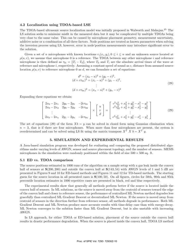
The TDOA-based ultrasonic source localization model was initially proposed in Walworth and Mahajan.25 TheLS solution seeks to minimize misfit in the measured data but it may be complicated by multiple TDOAs beingvery close to the same value. This can be caused by microphone placement geometry, measurement uncertainty,additive noise or a combination of all three factors. Node positions are treated as known parameters when solvingthe inversion process using LS, however, error in node‘position measurements may introduce significant error tothe solution.

Given a set of n microphones with known locations ri(xi, yi), 0 ≤ i ≤ n and an unknown source located atρ(u, v), we assume that microphone 0 is a reference. The TDOA between any other microphone i and referencemicrophone is then defined as τ0i = ‖Ti − T0‖, where T0 and Ti are the absolute arrival times of the wave atreference and microphone i, respectively. Assuming a constant speed of sound as c, distance from assumed sourcelocation ρ(u, v) to reference microphone 0 as d, we can formulate a set of equations:

d2 = (x0 − u)2 + (y0 − v)2,(d + cτ01)2 = (x1 − u)2 + (y1 − v)2,

...(d + cτ0n)2 = (xn − u)2 + (yn − v)2

(28)

Expanding these equations we obtain:⎡

⎢⎢⎢⎣

2x0 − 2x1 2y0 − 2y1 −2cτ01

2x0 − 2x2 2y0 − 2y2 −2cτ02

...2x0 − 2xn 2y1 − 2yn −2cτ0n

⎤

⎥⎥⎥⎦×⎡

⎣uvd

⎤

⎦ =

⎡

⎢⎢⎢⎣

c2τ201 + x2

0 + y20 − x2

1 − y21

c2τ202 + x2

0 + y20 − x2

2 − y22

...c2τ2

0n + x20 + y2

0 − x2n − y2

n

⎤

⎥⎥⎥⎦

(29)

The set of equations (29) of the form Xb = y can be solved in closed form using Gaussian elimination whenn = 3, that is if there are four microphones. When more than four microphones are present, the system isoverdetermined and can be solved using LS fit using the matrix transpose XT X b = XT y.

5. SIMULATION AND EXPERIMENTAL RESULTS

A Java-based simulation program was developed for evaluating and comparing the proposed distributed algo-rithms under varying levels of AWGN, sensor and source placement topology, and the number of sensors. MEMSmicrophones in the simulation were randomly positioned within the field of size 500× 500 sq. ft.

5.1 ED vs. TDOA comparison

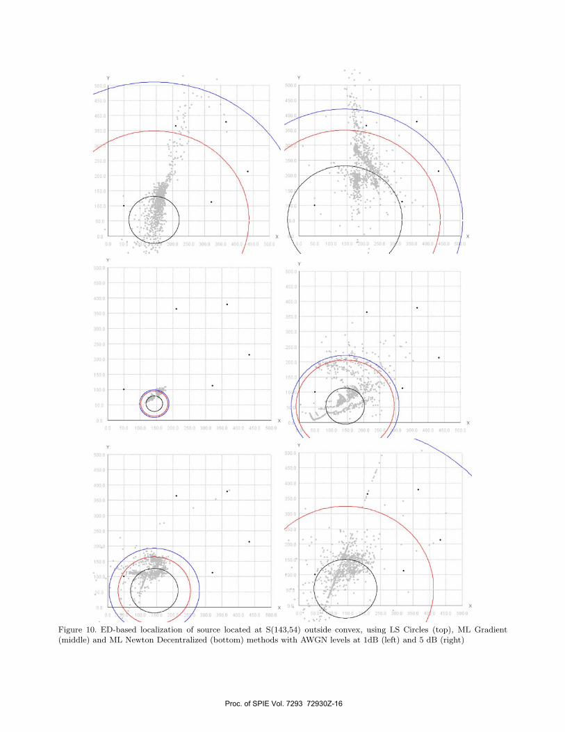
The source positions estimated in 1000 runs of the algorithm on a sample setup with a gas leak inside the convexhull of sensors at S(200, 200) and outside the convex hull at S(143, 54) with AWGN levels of 1 and 5 dB arepresented in Figures 9 and 10 for ED-based methods and Figures 11 and 12 for TD-based methods. The startingguess for the source location in all presented cases is S(100, 50). On all figures, circles for 50th, 90th and 95thpercentile location estimates in 1000 repetitive cases are presented in black, red and blue respectively.

The experimental results show that generally all methods perform better if the source is located inside theconvex hull of sensors. In ML solutions, as the source is moved away from the centroid of sensors toward the edgeof the convex hull and closer to reference sensor, the performance of centralized ML Newton method degrades lessgracefully than centralized ML Gradient Descent or decentralized ML Newton. If the source is moved away fromcentroid of sensors in the direction further from reference sensor, all methods degrade in performance. Both MLGradient Descent and ML Newton produce more accurate results with time-delay case than with energy-decay.ML Newton converges to the solution faster than ML Gradient Descent, but is also unstable with increasingAWGN.

In LS approach, for either TDOA or ED-based solution, placement of the source outside the convex hullresults in drastic performance degradation. When the source is placed inside the convex hull, TDOA LS method


e

\.p.

\O

- - --N -

U MICROPHONE SOURCE

outperforms ED LS method in accuracy with increasing AWGN, though evens out with the same accuracy atAWGN of 7 dB. The number of steps taken by each numerical method to localize the source to within the gradienttolerance of 0.25 are presented in Table 1 for ED-based localization and Table 2 for TDOA-based localizationwith two source placement options.

Table 1. Convergence of ED-based ML algorithms at ∇f(ρ) ≤ 0.25

ML Method S(200,200) S(143,54)

Gradient Descent 13 2Newton Centralized 4 2Newton Decentralized 8 7

Although the ML Gradient Descent method converges better in general, in cases where the source is locatedinside the convex hull of sensors, ML Newton method can achieve the same result 3 times faster. Clearlydecentralized ML Newton converges slower than centralized ML Newton, but it should be kept in mind that eachstep of centralized ML Newton requires SPL data from all sensors, while decentralized method uses only localSPL value at each sensor without extra communication. As shown by Rabbat and Nowak,18 such decentralizationalso offers significant savings in terms of complexity and power consumption.

Table 2. Convergence of TDOA-based ML algorithms at ∇f(ρ) ≤ 0.25

ML Method S(200,200) S(143,54)

Gradient Descent 16 7Newton Centralized 10 5

5.2 Testing with a nitrogen leak source

Figure 7. Test setup with nitrogen leak

We have also tested the decentralized ED-based ML Newton method in a 20 ft × 20 ft room with 4 MEMSmicrophone-mounted sensors arranged in a square as shown in Figure 7. Nitrogen gas was released from anorifice at 150 psi at four different locations inside the convex hull of the sensors. Raw signal data was sampled at200 kHz from the four sensors for periods ranging from 5 to 10 seconds using a National Instruments’ (NI) 16-bitdata acquisition card on a PC. The NI LabView program on the PC used this data to simultaneously computethe SPL readings at each microphone. The SPL data observed by the four microphones was fed as an input


( SUITE OF LOCALIZATION ALGORITHMS )

TIME-DELAYBASED

EXHAUSTIVESEARCH

HYPERBOLICINTERSECTION

LEASTSQUARES

FIT

GRADIENTDESCENT

ENERGY-DECAYBASED

CIRCLEINTERSECTION

NEWTONSMETHOD

SIGNALPHENOMENON

GEOMETRICREPRESENTA TION

NUMERICALMETHODS

INFORMATIONPROCESSING

SOURCETIME-DELAY TIME-DELAY ENERGY

ENERGYMLE EQUATIONS RATIO

MLE

into the Java-based program for localization. The application of decentralized ML Newton method resulted in asuccessful localization of the nitrogen leak source with an offset of less than 1 ft.

6. CONCLUSION AND FUTURE RESEARCH

We have developed and analyzed a suite of algorithms for localization of ultrasonic sources of gas leak usingdistributed MEMS microphones. The algorithms make use of the multiplicity of ultrasonic waves received atdistributed microphones observing a single source and estimate the source location using relative time delays(TDOA) or energy decays (ED). Apart from the algorithmic design, the application of MEMS microphones inthe context of a distributed localization of ultrasonic sources is novel on its own.

Figure 8 presents the classification of analyzed algorithms. The proposed localization schemes define ML

Figure 8. Classification and summary of analyzed algorithms

error functions based on either the differences in SPL values or in arrival times of the ultrasonic signal from asingle source at various sensor nodes. For the ED-based approach, we define the LS and ML models using SPLvariables measured in dB instead of an abstract definition of energy. Due to presence of AWGN in the input dataand background nuisance, we employed numerical approximation methods such as the steepest gradient descentand Newton’s method for converging to the ultrasonic ML solution. We also implemented LS-based methodsfor both ED-based and TDOA-based approaches, and drew comparisons in presence of the varying levels ofAWGN. The correctness of all implemented methods was verified using exhaustive search on the ML and LSerror functions.

In addition to centralized implementation, a decentralized implementation of the most efficient ED-based MLNewton method was developed. Experimental results indicate the advantage of using decentralized ML Newtonmethod for fast localization of sources located inside the convex hull of microphones. Although less precise thanML Gradient solution, decentralized ML Newton offers significant savings in power consumption due to lessernumber of convergence steps, hence - a lower communication overhead and better scalability, making this solutionmore attractive for a sensor network implementation.


Although the ED-based methods perform poorer in accuracy with increasing AWGN, they do not require ahigh-precision time synchronization like the TDOA-based methods do. The ED-based methods also involve lesscommunication overhead as a single sensor can produce a data observation (SPL), as opposed to TDOA-basedcases where a pair of sensors is needed to compute the time delay. These advantages make the ED-based methodsmore attractive for implementation in distributed sensor networks.

There are several directions for the future research on the subject of ultrasonic gas-leak localization usingdistributed sensor networks. Development of standardized network middleware for distributed ultrasonic local-ization would assist in the development of large and scalable clusters for detection of multiple gas leak sources atan industrial facility. Of particular interest in this case is the TinyOS operating system26, 27 for wireless sensornetworks, which already provides some necessary utilities and interfaces. Since the TinyOS was implementedover the Texas Instruments’ low-power MSP430 16-bit RISC microcontrollers,28 further research into hardwareintegration of MEMS microphones with this platform would be of interest as well.

In terms of distributed algorithms, the focus of future work could be on the development and performanceanalysis of the TDOA-based decentralized ML Newton as well as the high-precision clock mechanism for comput-ing time delays. TDOA methods which are not as efficient as ED-based methods can still offer a viable alternativein powered sensor networks. The application of microphone arrays21, 29 and beamforming techniques,30 in con-junction with the ultrasonic gas-leak localization using sensor networks is also an interesting future direction toexplore.

REFERENCES[1] Huseynov, J., Baliga, S., Dillencourt, M., Bic, L., and Bagherzadeh, N., “Energy-based localization of ultra-

sonic gas-leak sources using distributed MEMS microphones and a maximum-likelihood estimator,” in [the29th IEEE International Conference on Distributed Computing Systems (ICDCS) ], (June 2009 (submitted)).

[2] Van De Par, S., Schimmel, O., Kohlrausch, A., and Breebaart, J., “Source segregation based on temporalenvelope structure and binaural cues,” in [Hearing From Sensory Processing to Perception ], 143–153,Springer Berlin Heidelberg (2007).

[3] Guentchev, K. and Weng, J., “Learning-based three dimensional sound localization using a compact non-coplanar array of microphones,” in [1998 AAAI Symposium of Intelligent Environments ], (1998).

[4] Aarabi, P., “Robust multi-source sound localization using temporal power fusion,” in [Proceedings of SensorFusion: Architectures, Algorithms, and Applications V (Aerosense’01), Orlando, Florida ], (April 2001).

[5] Intanagonwiwat, C., Govindan, R., and Estrin, D., “Directed diffusion: A scalable and robust communica-tion paradigm for sensor networks,” in [Proceedings of the ACM/IEEE International Conference on MobileComputing and Networking ], 56–67 (2000).

[6] Pattem, S. and Zhao, F., “The impact of spatial correlation on routing with compression in wireless sen-sor networks,” in [Proceedings of the third international symposium on Information processing in sensornetworks, ], 28–35 (2004).

[7] Kumar, S., Zhao, F., and Shepherd, D., “Collaborative signal and information processing in microsensornetworks,” IEEE Signal Processing Magazine 19, 13–14 (2002).

[8] Akyildiz, I., Su, W., Sankarasubramaniam, Y., and Cayirci, E., “Wireless sensor networks: a survey,”Computer Networks 39, 393–422 (2002).

[9] Ilyas, M., Mahgoub, I., and Kelly, L., [Handbook of Sensor Networks: Compact Wireless and Wired SensingSystems ], ch. Dynamic Source Routing in Ad Hoc Wireless Networks, CRC Press (2004).

[10] Bian, X., Abowd, G. D., and Rehg, J. M., “Using sound source localization in a home environment,” LectureNotes in Computer Science 3468, 19–36 (2005).

[11] Widrow, B., Mantey, P., Griffiths, L., and Goode, B., “Adaptive antenna systems,” in [Proceedings of theIEEE ], 55, 2143–2159 (December 1967).

[12] Frost, O. L., “An algorithm for linearly constrained adaptive array processing,” in [Proceedings of the IEEE ],60, 926–935 (August 1972).

[13] Johnson, D. H. and Dudgeon, D. E., [Array Signal processing: Concepts and Techniques ], Prentice Hall(1993).


[14] Chen, J. C., Yip, L., Elson, J., Wang, H., Maniezzo, D., Hudson, R. E., Yao, K., and Estrin, D., “Coherentacoustic array processing and localization on wireless sensor networks,” in [Proceedings of the IEEE ], 91,1154–1162 (August 2003).

[15] GRAS, “Product data sheets and specifications.” http://www.gras.dk (2008).[16] MEMSTech, “Product data sheets and specifications.” http://www.memstech.com (2008).[17] Yonak, S. and Bowling, D., “Multiple microphone photoacoustic leak detection and localization system and

method,” (2001). U.S. Patent No. 6,227,036.[18] Rabbat, M. and Nowak, R., “Decentralized source localization and tracking,” in [Proceedings of the IEEE

International Conference on Acoustics, Speech, and Signal Processing (ICASSP’04) ], 3, 921–924 (2004).[19] Li, D. and Hu, Y. H., “Energy-based collaborative source localization using acoustic microsensor array,”

EURASIP Journal of Applied Signal Processing , 321–337 (2003).[20] Wang, S. and Yang, J., “Decentralized acoustic source localization with unknown source energy in a wireless

sensor network,” Measurement Science and Technology 18, 3768–3776 (2007).[21] Huang, Y., Benesty, J., and Chen, J., [Acoustic MIMO Signal Processing ], Springer Berlin Heidelberg

(2006).[22] Li, D. and Hu, Y. H., “Least square solutions of energy based acoustic source localization problems,” in

[Proceedings of the International Conference on Parallel Processing (ICPP) ], (August 2004).[23] Bickel, P. J. and Doksum, K. A., [Mathematical Statistics: Basic Ideas and Selected Topics ], Holden Day,

San Francisco (1977).[24] Champagne, B., Eizenman, M., and Pasupathy, S., “Exact maximum likelihood time delay estimation on

short observation intervals,” IEEE Transactions on Signal Processing 39, 285–298 (June 1991).[25] Walworth, M. and Mahajan, A., “An ultrasonic 3d position estimation system using the differences in the

time-of-flights from the transmitter to various receivers,” in [The 8th International Conference on AdvancedRobotics (ICAR’97) ], (1997).

[26] Levis, P. and Culler, D., “Mate: A Tiny Virtual Machine for Sensor Networks,” in [International Conferenceon Architectural Support for Programming Languages and Operating Systems ], (2002).

[27] UC Berkeley, “TinyOS - an open-source operating system designed for wireless embedded sensor networks.”http://www.tinyos.net (2004).

[28] Texas Instruments, “MSP430 low-power 16-bit risc microcontroller.” http://www.ti.com (2008).[29] Wax, M. and Kailath, T., “Optimum localization of multiple sources by passive arrays,” IEEE Transactions

on Acoustics, Speech and Signal Processing 31, 1210–1218 (1983).[30] Ward, D. B. and Elko, G. W., “Mixed nearfield-farfield beamforming: a new technique for speech acquisition

in reverberant environments,” in [the IEEE ASSP Workshop on Applied Signal Processing Audio Acoustics ],(1997).


oc

.0 00 4000 400 000

35:

30

1000

Y

I

00 500 000 50L 0 4000 4500 5000

S

5000

4500

4000

3500

3o0 0

250,0

2000

l500

000

500

00

300

100

L T i

.iu0 35O 1u 4UU

25 U

1000

TUU _UU UUO 3OUU OUUU 4UUU

350

1500

1000

UJU

Figure 9. ED-based localization of source located at S(200,200) inside convex, using LS Circles (top), ML Gradient(middle) and ML Newton Decentralized (bottom) methods with AWGN levels at 1dB (left) and 5 dB (right)


V

400

35Q L

150

100

50 U

0c4UUW 4UQ UUU

400 C

3500

3000

V

500

150

100

350

300

2500

2000

cn

0 1000 l50 3500 l000 4500 500O0

3500

:000

V

4000 4000 0000

V

500,:

450 C

4000

I co'

00

Figure 10. ED-based localization of source located at S(143,54) outside convex, using LS Circles (top), ML Gradient(middle) and ML Newton Decentralized (bottom) methods with AWGN levels at 1dB (left) and 5 dB (right)


V

5000

4500

4000

3500

3000 ---+----2500

1500 -

i000

500 4

0000 500 1000 1500 200

H t

300,0 3500 400,0 450 0 500 0

oo a

4500

400

3500

300

V

V

500 C

455

400

355

305

©

IOU

4

J 544 1000 1500 5u iUaO 3505 445u 4500 50044

000

450 0

400

350

3000

200

100 U

350

300

:50

200

050

0QP

oncp 000p ooc 000c jo: j

Do'

oc

Do

oc:

Figure 11. TDOA-based localization of source located at S(200,200) inside convex, using LS Equations (top), ML Gradient(middle) and ML Newton Centralized (bottom) methods with AWGN levels at 1dB (left) and 5 dB (right)


400 0

350.0

3000

250.0

2000

150.0

1000

50,0

00

V

00 50,0 100,0 1500 2000.2500 300,0 350,0 4000 4506

oo 0

450 C

400 0

350

300

000

1500

100

Y

1

- 3000 350 -oocp 000p o ocE

-t

4

A

oo

o oc

oo

0 000

x

000c ocp oQot a oaa

00

0 000

- 00p

00 V.

Figure 12. TDOA-based localization of source located at S(143,54) outside convex, using LS Equations (top), ML Gradient(middle) and ML Newton Centralized (bottom) methods with AWGN levels at 1dB (left) and 5 dB (right)


gas-leak localization using distributed ultrasonic sensorsbic/papers/spie.pdf · gas-leak...

Documents