gabriel katul, cheng-i hsieh and john sigmon50 gabriel katul et al. and x 3(= z) are the...

ENERGY-INERTIAL SCALE INTERACTIONS FOR VELOCITY ANDTEMPERATURE IN THE UNSTABLE ATMOSPHERIC SURFACE

LAYER

GABRIEL KATUL, CHENG-I HSIEH and JOHN SIGMONSchool of the Environment, Duke University, Durham, NC 27708-0328, U.S.A.

(Received in final form 16 July, 1996)

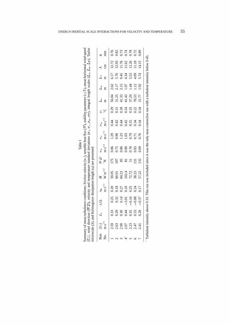
Abstract. Triaxial sonic anemometer velocity and temperature measurements were used to investigatethe local structure of the velocity and temperature fluctuations in the unstable atmospheric surfacelayer above a grass-covered forest clearing. Despite the existence of a 2/3 power law in the longitudinalvelocity (2 decades) and temperature (1 decade) structure functions, local isotropy within the inertialsubrange was not attained by the temperature field, although a near-isotropic state was attained by thevelocity field. It was found that sources of anisotropy were due to interactions between the large-scaleand small-scale eddy motion, and due to local velocity-thermal interactions. Statistical measureswere developed and used to quantify these types of interactions. Other types of interactions were alsomeasured but were less significant. The temperature gradient skewness was measured and found tobe non-zero in agreement with other laboratory flow types for inertial subrange scales. Despite theseinteractions and anisotropy sources in the local temperature field, Obukhov’s 1949 hypothesis forthe mixed velocity-temperature structure functions was found to be valid. Finally, our measurementsshow that while a 2/3 power-law in the longitudinal velocity structure function developed at scalescomparable to five times the height from the ground surface (z), near-isotropic conditions wereachieved at scales smaller than z/2.

1. Introduction

Numerous field and laboratory experiments demonstrate that velocity and temper-ature measurements in the atmospheric surface layer (ASL) exhibit an extensiveinertial subrange, whose signature is commonly associated with a �5/3 powerlaw in the spectral density function. Within the inertial subrange, turbulent kineticenergy per unit mass (TKE) is neither produced nor dissipated but simply cas-cades down to smaller scales by vortex stretching. An important statistical propertyof the inertial subrange is the locally isotropic nature of the eddy motion. Thisisotropy permits simplifications to the dynamical description of these scales ofmotion according to Kolmogorov’s (1941) original theory (hereafter referred to asK41).

A wide inertial subrange in the ASL is attributed to the large-scale separa-tion between turbulent production (mechanical and buoyant) at Lu and viscousdissipation at �. In this study, Lu is the integral length scale of the longitudinalvelocity fluctuations, � (=[�3=h�i]1=4) is the Kolmogorov microscale, � (= 1.5� 10�5 m2 s�1) is the kinematic viscosity of air, � (=�[@ui=@xj + @uj=@xi]

2)is the turbulent kinetic energy dissipation rate per unit mass, ui is the turbulentvelocity fluctuation component (u1 = u, u2 = v, and u3 = w), x1(=x), x2(=y),

Boundary-Layer Meteorology 82: 49–80, 1997.c 1997 Kluwer Academic Publishers. Printed in the Netherlands.

50 GABRIEL KATUL ET AL.

and x3(=z) are the longitudinal, lateral, and vertical directions, respectively (inthis study, both meteorological and tensor notations are used), and h:i is the timeaveraging operator (assumed to be identical to the ensemble averaging operator bythe ergodic hypothesis as discussed in Monin and Yaglom, 1971; Ch. 2; Lumleyand Panofsky, 1964). This wide separation between Lu and � (for many unstableASL flows Lu=� � 105) ensures that the transfer of TKE (= TE), from productionto dissipation, cascades over many intermediate scales. Hence, it is expected that allanisotropy in the eddy motion associated with the turbulent production (mechanicalor thermal) at Lu will diminish during this energy cascade process.

Air-temperature time series measurements in the ASL clearly exhibit welldefined large-scale structures (e.g. temperature ramps) whose length scales arecomparable or larger than Lu. The sharp edges of these structures, characterizedby a large and rapid change in temperature over a very short time duration, maycontribute directly to Fourier amplitudes at higher wavenumbers without manyintermediate cascade steps, as evidenced by Mahrt (1989). Hence, when thesestructures exist, the inertial subrange eddy motion (hereafter referred to as smallscale) may be contaminated by the larger scale organized eddy motion due to a“short circuiting” in the energy-cascade. While this non-local energy transfer isattributed to the rapid drop at the ramp-edge, other studies demonstrated that theramp slopes are of significance. For example, Van Atta (1977) showed that theramp-like structures in the temperature significantly contribute to the non-zero val-ues of the odd-ordered temperature structure functions in agreement with Gibsonet al. (1977). Based on local isotropy predictions, these odd-ordered temperaturestructure functions must be identically zero for all separation distances withinthe inertial subrange. To explain the non-zero behavior of the odd-ordered tem-perature structure functions, Van Atta (1977) proposed an idealized ramp modelthat implicitly assumes organized motion with ramp-like signatures influence theinertial subrange statistics of the temperature field.

Irrespective of the anisotropy source (ramp slope or edge), if interactionsbetween large scales and small scales are significant, then it is possible that theanisotropy of the large scales persists in the inertial subrange, and key assumptionsregarding i) isotropy, ii) the universal nature of the power-laws within the iner-tial subrange, (e.g. Kuznetsov et al., 1992), and iii) Obukhov’s constant structureskewness hypothesis (Obukhov, 1949; Katul et al., 1994a) are violated and requirere-examination for ASL flows. If such interactions are important, then the structureof the inertial subrange may not be universal since the larger scale eddy motions arestrongly influenced by the boundary conditions imposed by the land-atmosphereinterface or the existing atmospheric stability conditions. For the purpose of thisstudy, large scales are eddies with characteristic length scales�Lu and small scalesare eddies with scales much larger than � but much smaller than the height abovethe ground surface (z).

The objective of this study is to investigate the influence of such interactions onthe Kolmogorov inertial scale eddy motion close to the land-atmosphere interface

ENERGY-INERTIAL SCALE INTERACTIONS FOR VELOCITY AND TEMPERATURE 51

using velocity and temperature time series measurements within the ASL. Specialattention is paid to the local velocity-thermal interaction, an interaction that wasinvestigated by Antonia and Van Atta (1975, 1978), Antonia and Chambers (1980),and recently by Antonia and Zhu (1994) who measured non-zero amplitudes in thelongitudinal heat flux co-spectrum within the inertial subrange.

For that purpose, 56 Hz triaxial sonic anemometer velocity and temperaturemeasurements were carried out in the ASL above a grass-covered forest clearing inDurham, North Carolina for a wide range of atmospheric stability conditions. Ourspecific objectives are to investigate how energy containing small-scale interactionsand local velocity-thermal interactions modify i) K41 power-laws, ii) Obukhov’sconstant skewness hypothesis, and iii) the isotropic state of the small-scale eddymotion in the ASL. Since K41 and Obukhov’s constant skewness hypothesis weredeveloped for the velocity and temperature differences between two neighbouringpoints, the structure function approach is utilized throughout.

2. Theory

The equations relating the second (Duu(r)) and third (Duuu(r)) order structurefunctions, and the mixed velocity-temperature (DTTu(r)) and second order tem-perature (DTT (r)) structure functions, as derived from the Navier–Stokes (NS)equations for locally isotropic turbulence, are given by

Duuu(r)� 6�ddrDuu(r) = �4

5h�ir

DTTu(r)� 2�ddrDTT (r) = �4

3hNT ir

(1)

where Duuu(r) = h[u(x + r) � u(x)]3i, Duu(r) = h[u(x + r)� u(x)]2i, DTT (r)= h[T (x+ r)� T (x)]2i, DTTu(r) = h[T (x+ r)� T (x)]2[u(x+ r)� u(x)]i, NT

is one half the temperature variance dissipation rate, � is the molecular diffusivityfor heat, and r is the separation distance along the longitudinal direction (seeMonin and Yaglom, 1975, p. 401–403 for derivation). In deriving Equation (1), itis assumed that the Reynolds and Peclet numbers are very large, the statistical stateof the small-scale eddies (e.g. scales much smaller thanLu) are independent of themacro-structural flow properties, and that the temperature and velocity differences(�T and �u), for r much less than Lu and LT , are independent. Here, LT isthe temperature integral length scale. That is, at the small scales, temperature isa passive scalar and does not interact locally with the longitudinal velocity field.Throughout this study, we will assume that at any time instant (t), the longitudinalvelocity (U ) and air temperature (Ta) can be decomposed, without ambiguity, intotime averages (hUi, hT i) and fluctuations about these time averages (u, T ). Thus,at time t, U(t) = hUi+ u(t) and Ta(t) = hT i+ T (t), and huii = 0.


An important asymptotic result that follows from Equation (1) is the behaviorof Duuu(r) and DTTu(r) in the limit when r � � and � is very small. This isgiven by

Duuu(r) ' �45h�ir

DTTu(r) ' �43hNT ir

(2)

which agrees well with K41 (=Cn(h�ir)n=3) predictions for the third order(n = 3) longitudinal velocity structure function withC3 = �4=5. Obukhov (1949)suggested that the following dimensionless quantities

S(r) =Duuu(r)

[Duu(r)]3=2

F (r) =DTTu(r)

DTT (r)[Duu(r)]1=2

(3)

to be constants independent of r in order to recover K41 predictions for Duu(r)and DTT (r) from Duuu(r) and DTTu(r) (see also Monin and Yaglom, 1975 pp.397–400). These constants were determined experimentally to be S(r) = �0:25and F (r) = �0:4 and were also related to the Kolmogorov constant as discussedin Katul et al. (1995a). Notable exceptions to these experimental values are dueto Kerr (1985, 1990) who found S(r) = �0:4 and F (r) = �0:5 using a directnumerical simulation for isotropic turbulence (see also Gibson et al., 1988). Also,the �0.4 value for F (r) is not consistent with the accepted Kolmogorov constantfor the second order temperature structure function CT = 3:2 (see Kaimal andFinnigan, 1994; p. 52).

3. Experimental Setup

The measurements were carried out on July 12–16, 1995 at 5.2 m above the groundsurface over an Alta Fescue grass site at the Blackwood division of the DukeForest in Durham, North Carolina. During this time period, a heat wave residedin North Carolina for several days after it had swept from the midwest to the eastcoast. During the experiment, maximum mean air temperatures up to 38 �C weremeasured in Durham. The sky condition during these five days was clear with lowto moderate winds.

The site is a 480 m by 305 m grass-covered forest clearing (site elevation= 163 m), and a mast, situated at 250 m and 160 m from the north-end andwest-end portions of a 10 m Loblolly pine forest edge respectively, was used


to mount a triaxial sonic anemometer. The three velocity components (U1, U2,U3) and air temperature were measured using a triaxial ultrasonic anemometer(Gill Instruments/1012R2). Sonic anemometers measure the velocity by sensingthe effect of wind on the transit times of sound pulses travelling in oppositedirections across a known instrument path distance dsl( = 0.149 m in this study).A key disadvantage of sonic anemometers is the wavenumber (K) distortion dueto averaging along the finite sonic path dsl. This distortion is limited to separationdistances r � dsl or K � d�1

sl(Wyngaard, 1981; this limit was erroneously quoted

in Katul et al., 1995a,b as K � 2�d�1sl

instead of K � d�1sl

for K in rad s�1). Thesampling frequency (fs) and the sampling period (Tp) were 56 Hz and 19.5 minutesrespectively, resulting in N = 65,536 measurements per velocity component. The56 Hz sampling frequency is the maximum achievable frequency by the Gill sonicanemometer and is used in this experiment. The Gill anemometer was calibratedat the Department of Aeronautics and Astronautics wind-tunnel facility (2.1 m �1.5 m � 4.4 m) at Southampton University and tested for any transducer delaysand flow distortions. Taylor’s (1938) frozen turbulence hypothesis was used toconvert time increments to space increments (r = �hUit). Since some averagingoccurs for r < dsl, the statistical analysis is limited to r > dsl but the full range ofstructure function measurements is shown.

From the 5-day experiment, more than 120 runs were collected. After inspection,only 6 runs were used in this study, which exhibited i) at least one decade of inertialsubrange as identified by the 2/3 power law in the longitudinal velocity structurefunction, ii) a temperature standard deviation (�T ) in excess of 0.2 �C to insureadequate thermal agitation, iii) clear and identifiable time averages (hUi and hT i)to permit decomposition into a mean and a fluctuating part without ambiguity,and iv) a turbulent intensity Iu(= �u=hU1i, where �u is the root-mean squaredlongitudinal velocity) not exceeding 0.33 to minimize distortions resulting fromTaylor’s (1938) frozen turbulence hypothesis. Due to the low wind speeds duringthe 5-day period, Iu was greater than 0.3 for the majority of runs. For 30 runs,the wind speeds at 5.2 m were below 1.5 m s�1. For near convective conditions,none of the runs had an Iu < 0:33 and we used the run with the smallest turbulentintensity (Iu = 0:44). Therefore, the total number of runs from this experiment is7.

While the limiting Iu = 0:33 is well within the criteria set by Stull (1988 p.6), this intensity is not very small (e.g. I2

u = 0:1) as evidenced by Lin (1953).We still employed Taylor’s (1938) frozen turbulence hypothesis assuming thatit is at least valid for the small-scale eddy motion within the inertial subrange.Powell and Elderkin (1974) and Mizuno and Panofsky (1975) did demonstrate thatLin’s (1953) criterion (I2

u � 0:1) is too limiting for the ASL and can be relaxedfor operational purposes. Despite an I2

u = 0:09, they found that Taylor’s (1938)frozen turbulence hypothesis is valid for scales in excess of 250 m. We note thatdistortions at the small scales in high intensity shear flow can be severe, as shownby the experiments of Fisher and Davies (1964). A potential assessment of these


distortions is presented in the following section using the model by Wyngaard andClifford (1977).

The absolute air temperature was determined from the speed of sound cs using

c2s = �RdTa (4)

where Rd (=287.04 J Kg�1 K�1) is the gas constant of dry air at constant pressure,and �(= 1.4) is the ratio of the molar specific heat capacities of air at constantpressure to that at constant volume. It should be noted that the spatial averagingof the sonic anemometer for temperature readings are compatible with those forvelocity. However, the temperature measurements are also contaminated by resid-ual sensitivities to humidity. This was the main reason for considering runs with�T > 0.2 �C to ensure that the temperature perturbations are large enough to bewell detected by the sonic anemometer and we neglect the secondary humiditycorrections to the temperature measurements (see also Kaimal, 1986). A compari-son between the Gill temperature fluctuations and a Campbell Scientific fine wirechromel-constantan thermocouple is discussed in Appendix A. Good agreementbetween the temperature measurements from both instruments is noted in AppendixA. The characteristic turbulence length scales are summarized in Table I, where thelongitudinal (Lu) and vertical (Lw) velocity, and temperature (LT ) integral lengthscales, the Taylor microscale (�), and � were estimated from

LT =hUihT 2i

Z1

0hT (t+ �)T (t)id�

Lui=hUihu2

ii

Z1

0hui(t+ �)ui(t)id� i = 1; 3

� = �u

s15

�

h�i

� =

�3

h�i

!1=4

(5)

(see Tennekes and Lumley, 1972 pp. 66–67). For determining Lu, Lw and LT ,the integration of the autocorrelation function was carried out up to the first zerocrossing (see Sirivat and Warhaft, 1983). From Table I, the mean Lw and Lu are2.0 m and 40.0 m, respectively, and are in excellent agreement with the estimatesby Kader et al. (1989) who found Lu=Lw = 20:6. Due to the limited spatial reso-lution of sonic anemometers, the mean dissipation rate was not directly measured.However, h�i was estimated using two methods: i) similarity theory in conjunctionwith the steady state assumption that TE = h�i, and ii) the third order structurefunction. These methods are discussed next:


Tabl

eI

Sum

mar

yof

mea

ntu

rbul

ence

cond

itio

ns:f

rict

ion

velo

city

( u�

),se

nsib

lehe

atflu

x(H

),st

abili

typa

ram

eter

(z=L

),m

ean

hori

zont

alw

ind

spee

d

hU

1

i,w

ind

dire

ctio

n(W

D

),ve

loci

tyan

dte

mpe

ratu

rest

anda

rdde

viat

ions

(�u;�v;�w;�T

),in

tegr

alle

ngth

scal

es(L

u;Lw;LT

),Ta

ylor

mic

rosc

ale

(�

),an

dK

olm

ogor

ovdi

ssip

atio

nle

ngth

(�

)ar

epr

esen

ted

Run

hU

1

i

I u

z=L

u�

H

WD

�u

�v

�w

�t

Lu

Lw

LT

�

�

No.

ms�

1m

s�

1W

m

�

2

�

Nm

s�

1m

s�

1m

s�

1

�

Cm

mm

cmm

m

12.

590.

33

�

0.25

0.20

59.0

517

50.

861.

290.

440.

2956

.04

2.62

6.17

12.7

20.

762

2.63

0.29

�

0.32

0.18

60.0

110

70.

750.

960.

420.

3131

.25

2.17

5.76

12.9

30.

823

2.90

0.30

�

0.14

0.27

84.2

385

0.86

1.23

0.44

0.39

41.3

32.

159.

4511

.76

0.73

4�

2.07

0.44

�

3.01

0.10

102.

481

0.90

1.03

0.42

0.54

41.4

31.

974.

3411

.62

0.74

52.

230.

35

�

0.16

0.25

72.7

251

0.78

0.79

0.35

0.35

37.2

91.

445.

5312

.26

0.78

62.

470.

33

�

0.08

0.24

38.2

313

10.

830.

710.

340.

2278

.53

1.12

4.09

11.1

80.

727

2.41

0.28

�

0.37

0.17

57.2

213

50.

690.

760.

340.

3431

.77

1.92

5.74

14.1

50.

89

�

Tur

bule

ntin

tens

ity

abov

e0.

33.T

his

run

was

incl

uded

sinc

eit

was

the

only

near

-con

vect

ive

run

wit

ha

turb

ulen

tint

ensi

tybe

low

0.45

.


(i) Similarity TheoryThe mean dissipation rate can be estimated from

h�i =��

�z

L

��u3�

kz(6)

where u�(= h�uwi1=2) is the friction velocity, z (= 5.2 m) is the height above theground surface, and L is the Obukhov length given by

L = � �u3�

kg

H

cpTa

! (7)

where H(= �cphwT i) is the sensible heat flux, and �� is the dissipation stabilitycorrection function (see Panofsky and Dutton, 1984 p. 180; Brutsaert, 1982 p. 193for a review) given by the following empirical relations:

�� = 1� z

L;

�z

L< 0

�

�� = �m �z

L; �m =

�1� 16

z

L

��1=4

;��2 <

z

L< 0

�

�� =

1 + 0:5

�� zL��2=3

!3=2

:

��2 <

z

L< 0

�(8)

Hence, from measured u� and H , h�i can be determined for all dissipation stabilitycorrection functions; comparisons are shown in Table II.

(ii) The Third Order Structure FunctionThe mean dissipation rate was also determined from the measured third orderstructure function using the following procedure:(1) Utilize the dependence ofDuuu(r) (= �4=5h�ir) on r to determine the extent

of the inertial subrange, if it exists.(2) Fit a linear regression model of the form Duuu(r) = Ar and determine the

slope (A) using linear regression analysis.(3) Compute h�i from the slope A (determined from linear regression analysis in

step 2) using h�i = �5A=4.A similar procedure was used to estimate h�i from the measured Duu(r) and

the Kolomogorov constant (C2 = 2.2; see Kaimal and Finnigan, 1994 pp. 63–64).These estimates of h�i are compared to the estimates from method (i) in Table II. Allmethods result in comparable estimates of the mean dissipation rate, at least for thepurpose of this study. We decided to use the estimated h�i fromDuuu for computing


Table IIComparison between the estimated mean dissipation rates (m2 s�3) using sim-ilarity theory and the structure function approaches. The estimated dissipationsusing similarity theory are for the suggested stability correction functions. Thesubscripts 1, 2, and 3 are for the stability correction functions in Equation (8)starting from top to bottom, respectively. For the purpose of this study, thedissipation rates estimated from Duuu are used to calculate � and � in Table I

Similarity theory Structure functionRun no. h�i1 h�i2 h�i3 h�i from Duu h�i from Duuu

1 0.0045 0.0033 0.0047 0.0096 0.01032 0.0038 0.0027 0.0039 0.0089 0.00763 0.0103 0.0080 0.0109 0.0087 0.01204� 0.0021 0.0018 0.0015 0.0083 0.01155 0.0082 0.0063 0.0087 0.0057 0.00916 0.0075 0.0062 0.0079 0.0064 0.01237 0.0032 0.0023 0.0033 0.0056 0.0053

� Turbulent intensity above 0.33. This run was included since it was the onlynear-convective run with a turbulent intensity below 0.45. Also, z=L is outsidethe range of stability conditions in (8).

� since this dissipation method does not involve any assumption regarding planarhomogeneity of the turbulence statistics (as in similarity theory) and is insensitiveto the value of the Kolmogorov constantC2 (as in Duu). In this study, turbulence isconsidered to be planar homogeneous if the turbulence statistics do not vary in thelongitudinal or lateral directions. The following analysis does not require explicitmeasures of h�i and we only report the dissipation rate here for calculating � and �and qualitatively compare our results with other ASL and laboratory studies whichreport the Taylor microscale Reynolds number (Re = ��u=�).

Using this estimate of h�i, � and � were computed from Equation (5). Also, fora qualitative order of magnitude evaluation, they were compared to ASL measure-ments by Bradley et al. (1981; Table I). For � and �, Bradley et al. (1981) reporta range from 0.056 m to 0.137 m and from 0.38 mm to 0.85 mm, respectively.It is interesting to note that the Bradley et al. (1981) measurements were carriedout using a non-linearized DISA constant-temperature hot wire anemometer witha sampling frequency of 100 Hz. In their study, h�i was evaluated directly fromthe local isotropy relation in Tennekes and Lumley (1972 pp. 66; equation 3.2.9).These ranges are very similar to our indirect estimates in Table I. What is impor-tant to note from these estimates is that i) the termination of the inertial subrange,calculated by Praskovsky et al. (1993) to be 30�, is on the order of 3 cm and is wellbelow the sonic anemometer path length, ii) separation distances close to dsl maybe comparable to �, and iii) the Taylor microscale Reynolds number (see Table III)is well above 2,000, and the temperature field should achieve a near-isotropic statefor small separation distances (see Jayesh et al., 1994).


Table IIISummary of temperature and temperature gradi-ent skewness. The longitudinal velocity skewnessis also shown.

Run # hT 3i=(�3T ) Re = �u�=� jST j

1 0.97 7,300 0.52 1.14 6,465 0.733 1.19 6,742 0.834� 1.08 7,572 0.885 0.43 6,375 0.806 0.45 5,187 0.717 0.63 6,507 0.58

� Turbulent intensity above 0.33. This run is inexcellent agreement with the data by Gibson etal. (1977) for strongly unstable atmospheric con-ditions.

4. Results and Discussion

This section is divided into three parts, the first part discusses the extent of theinertial subrange and the onset of local isotropy, the second part presents the mea-sured deviations from the Kolmogorov– Obukhov structure function equations andObukhov’s (1949) hypothesis, the third part discusses these deviations within thecontext of large-scale/small-scale interactions and velocity-temperature interac-tions originally proposed in Praskovsky et al. (1993).

For the later purpose, the characteristic velocity of the small-scale eddy motion,defined within a sphere whose radius is r(�Lu), is �u (see also Frisch et al.,1978; Monin and Yaglom, 1975 Ch. 8; Landau and Liftshitz, 1986 pp. 129–135;Katul et al., 1995a,b). This scale is consistent with K41 since the dissipation rate,which defines all the velocity statistical properties within the inertial subrange,is on the order of �u3=r thus making �u the appropriate small-scale velocity.Furthermore, it was shown in Praskovsky et al. (1993; Figures 8–10) that the large-scale characteristic velocity at a point is u. This velocity scale is consistent withthe notion that at a point in the fluid, the amplitude of the turbulent perturbation isdue to large-scale eddies. In this study, we assume that the same arguments holdfor thermal perturbations.

4.1. IDENTIFICATION OF THE INERTIAL SUBRANGE AND THE ONSET OF LOCALISOTROPY

The identification of the inertial subrange is not a straightforward task given thewide range of tests and the different sensitivity levels of each test (see Antonia etal., 1986 and Antonia and Kim, 1994). Saddoughi and Veeravalli (1994) presented


several methods to identify the low frequency limit at which an isotropic state inthe velocity time series is achieved. They noted very different limits dependingon the turbulent statistic being analyzed. In their study, the shear stress cospectraldensity function approached zero at wavenumbers about a decade larger thanthat at which the energy spectra first followed a �5/3 power law. Based on theKansas experiments, Kaimal et al. (1972) found that the onset of local isotropy, asmeasured by the ratio of the vertical to the longitudinal velocity power spectrum,occurs at scales comparable to z. Their data show that for near-neutral conditions,the onset of local isotropy occurs at scales comparable to 0.5z (see also Kaimal,1986). However, their data show a �5/3 power-law in the longitudinal velocitypower spectrum at scales 5 times larger than z. The Praskovsky et al. (1993) datademonstrated that the inertial subrange, as identified by the third-order structurefunction, is between 30 � and Lu/8. Kader et al. (1989) found that Lu= 10.3z inthe ASL, implying that the upper scale limit of Praskovsky et al. (1993) is about1.3z, which agrees with a 2�z/4.5 theoretical estimate by Pond et al. (1963). Asurvey of isotropic limits from many other laboratory and ASL studies is presentedin Monin and Yaglom (1975, pp. 453–458).

Since the structure function approach is used throughout this study, the relationsbetween the vertical, lateral, and longitudinal velocity structure functions for locallyisotropic turbulent flows are given by

Dww(r)

Dvv(r)=h(W (x+ r)�W (x))2ih(V (x+ r)� V (x))2i = 1

Duu(r)

Dww(r)=h(U(x+ r)� U(x))2ih(W (x+ r)�W (x))2i =

34

(9)

where Dww(r) and Dvv(r) are the vertical and lateral velocity structure functions,respectively (see Monin and Yaglom, 1975 pp. 461). The above relations wereused to investigate the inertial subrange isotropy rather than the ratio of the powerspectra since for each separation distance (r), the structure function is calculatedfrom at least 50,000 data points. In contrast, the average Fourier amplitudes foreach wavenumber is calculated from a limited number of windows, and thus isnoisier for the purpose of our study.

Also, the ratios in Equation (9) are less sensitive to possible distortion by Taylor’s(1938) frozen turbulence hypothesis when compared to the�5/3 power-law in theindividual longitudinalEuu, lateral Evv , and vertical Eww velocity spectra. Noticein Equation (9) that any distortion caused by Taylor’s (1938) hypothesis affectsboth the numerator and the denominator, and thus has less influence on theirratio, especially the lateral and vertical structure functions. In Figures 1a and 1b,the measured ratios in Equation (9) are presented for all seven runs. The lowerscale limit is based on Wyngaard’s (1981) sonic-anemometer distortion criteria(r = dsl) and the upper limit is based on the Kaimal et al. (1972) data for near-


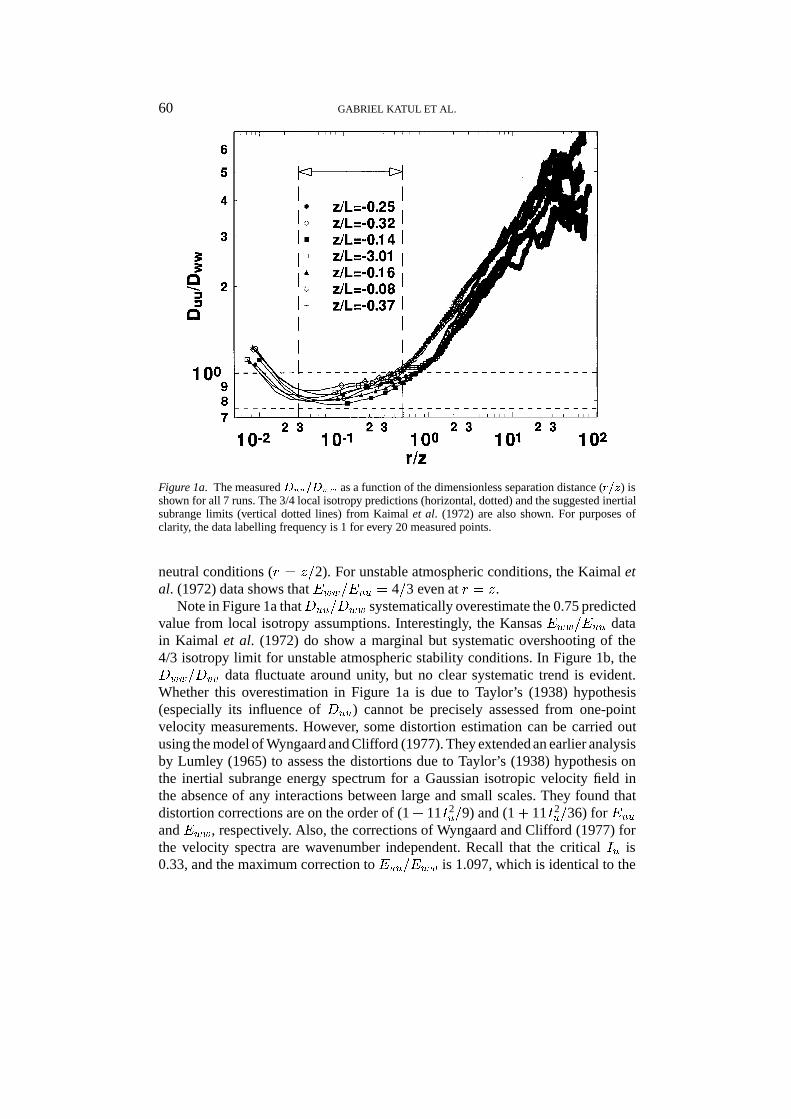
Figure 1a. The measured Duu=Dww as a function of the dimensionless separation distance (r=z) isshown for all 7 runs. The 3/4 local isotropy predictions (horizontal, dotted) and the suggested inertialsubrange limits (vertical dotted lines) from Kaimal et al. (1972) are also shown. For purposes ofclarity, the data labelling frequency is 1 for every 20 measured points.

neutral conditions (r = z=2). For unstable atmospheric conditions, the Kaimal etal. (1972) data shows that Eww=Euu = 4=3 even at r = z.

Note in Figure 1a thatDuu=Dww systematically overestimate the 0.75 predictedvalue from local isotropy assumptions. Interestingly, the Kansas Eww=Euu datain Kaimal et al. (1972) do show a marginal but systematic overshooting of the4/3 isotropy limit for unstable atmospheric stability conditions. In Figure 1b, theDww=Dvv data fluctuate around unity, but no clear systematic trend is evident.Whether this overestimation in Figure 1a is due to Taylor’s (1938) hypothesis(especially its influence of Duu) cannot be precisely assessed from one-pointvelocity measurements. However, some distortion estimation can be carried outusing the model of Wyngaard and Clifford (1977). They extended an earlier analysisby Lumley (1965) to assess the distortions due to Taylor’s (1938) hypothesis onthe inertial subrange energy spectrum for a Gaussian isotropic velocity field inthe absence of any interactions between large and small scales. They found thatdistortion corrections are on the order of (1 + 11I2

u=9) and (1 + 11I2u=36) for Euu

and Eww, respectively. Also, the corrections of Wyngaard and Clifford (1977) forthe velocity spectra are wavenumber independent. Recall that the critical Iu is0.33, and the maximum correction to Euu=Eww is 1.097, which is identical to the


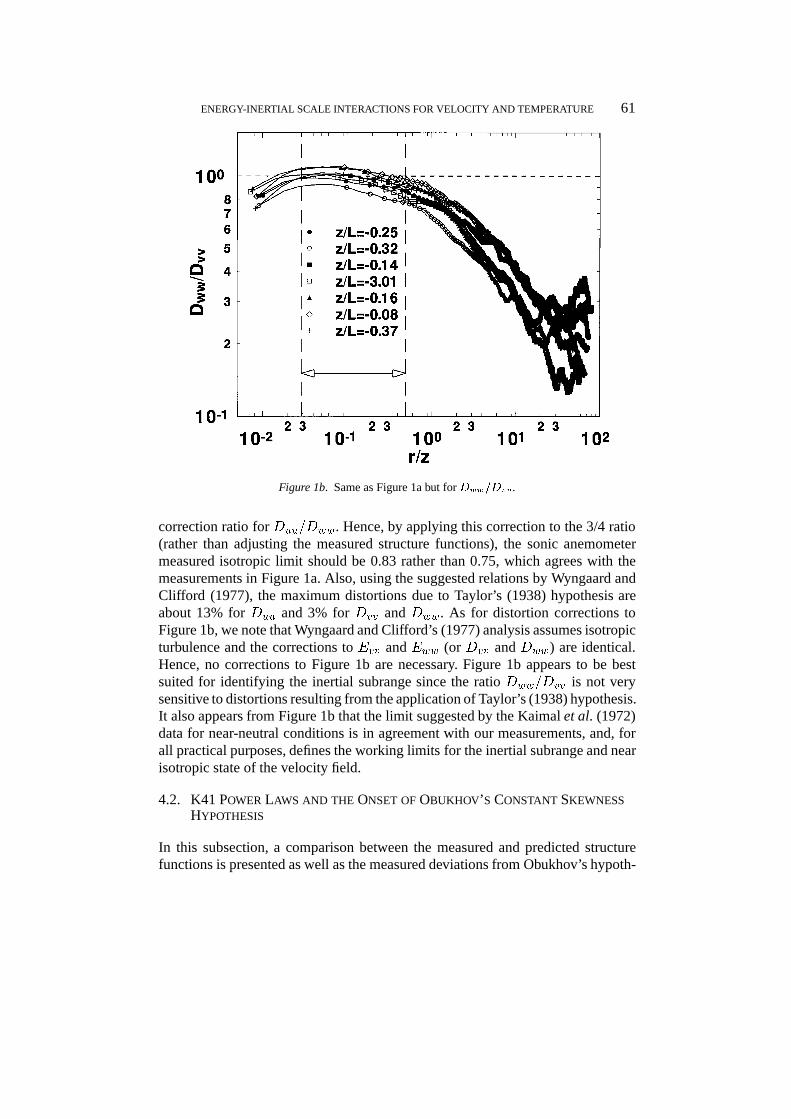
Figure 1b. Same as Figure 1a but for Dww=Dvv .

correction ratio for Duu=Dww. Hence, by applying this correction to the 3/4 ratio(rather than adjusting the measured structure functions), the sonic anemometermeasured isotropic limit should be 0.83 rather than 0.75, which agrees with themeasurements in Figure 1a. Also, using the suggested relations by Wyngaard andClifford (1977), the maximum distortions due to Taylor’s (1938) hypothesis areabout 13% for Duu and 3% for Dvv and Dww. As for distortion corrections toFigure 1b, we note that Wyngaard and Clifford’s (1977) analysis assumes isotropicturbulence and the corrections to Evv and Eww (or Dvv and Dww) are identical.Hence, no corrections to Figure 1b are necessary. Figure 1b appears to be bestsuited for identifying the inertial subrange since the ratio Dww=Dvv is not verysensitive to distortions resulting from the application of Taylor’s (1938) hypothesis.It also appears from Figure 1b that the limit suggested by the Kaimal et al. (1972)data for near-neutral conditions is in agreement with our measurements, and, forall practical purposes, defines the working limits for the inertial subrange and nearisotropic state of the velocity field.

4.2. K41 POWER LAWS AND THE ONSET OF OBUKHOV’S CONSTANT SKEWNESSHYPOTHESIS

In this subsection, a comparison between the measured and predicted structurefunctions is presented as well as the measured deviations from Obukhov’s hypoth-


Figure 2a. The second-order structure function (Duu(r)) as a function of the dimensionless separationdistance (r=z). The 2/3 power law is also shown (solid). For purposes of clarity, the data labellingfrequency is 1 for every 20 measured points.

esis for velocity and temperature. Figures 2a and 2b display the measured secondorder structure functions for velocity and temperature respectively, for all sevenruns. In both figures, it is apparent that for separation distances r < dsl, the mea-suredDuu(r) andDTT (r) slopes are steeper than K41 predictions due to the addeddissipation by instrument volume averaging along dsl. For r > dsl, Duu exhibiteda 2/3 power law consistent with K41 for at least r > 5z. This upper limit is inagreement with the limit found in Katul et al. (1995a,b) using Duuu(r). The DTT

in Figure 2b do not exhibit an extensive 2/3 power law (r = z) when compared toDuu(r > 5z) in Figure 2a.

In order to assess Obukhov’s (1949) hypothesis, the measured S(r) and F (r)are plotted against r=z for all runs in Figures 2c and 2d respectively. Notice thatthe scatter in Figure 2c is larger than the 0.22–0.3 variability reported from manylaboratory experiments (see e.g. Townsend, 1976 pp. 98–99; Monin and Yaglom,1975 pp. 471–473; Landau and Lifshitz, 1987 p. 145) but no consistent trend (i.e.overestimation or underestimation) is apparent. In this case, the scatter may beattributed to the limited sample size (N = 65,536) necessary to ensure convergencefor Duuu(r). The average S(r) from these seven runs is �0.2, which is in closeagreement with the S(r) = �0:25 (dotted line) derived from the Kolmogorovconstant in Katul et al. (1995a; Appendix 3).


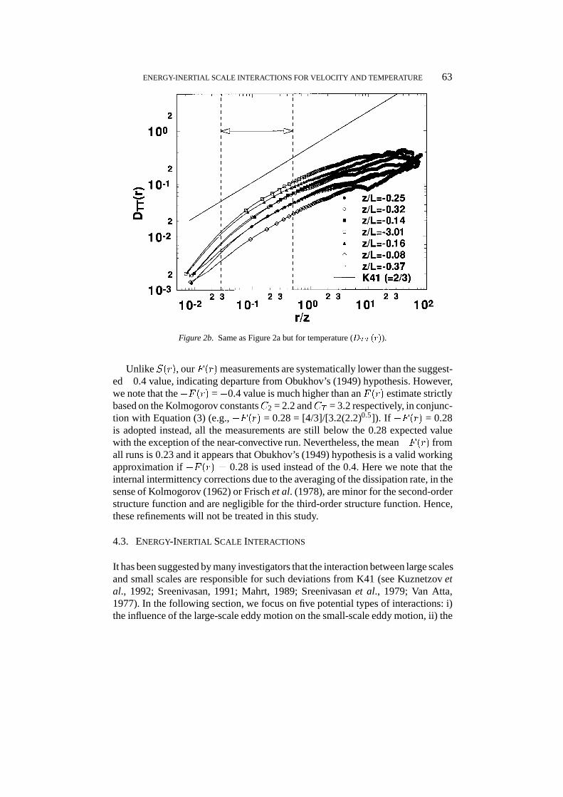
Figure 2b. Same as Figure 2a but for temperature (DTT (r)).

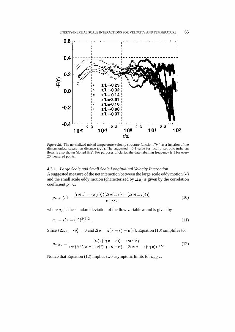
Unlike S(r), our F (r) measurements are systematically lower than the suggest-ed �0.4 value, indicating departure from Obukhov’s (1949) hypothesis. However,we note that the�F (r) =�0.4 value is much higher than an F (r) estimate strictlybased on the Kolmogorov constantsC2 = 2.2 andCT = 3.2 respectively, in conjunc-tion with Equation (3) (e.g., �F (r) = 0.28 = [4/3]/[3.2(2.2)0:5]). If �F (r) = 0.28is adopted instead, all the measurements are still below the 0.28 expected valuewith the exception of the near-convective run. Nevertheless, the mean�F (r) fromall runs is 0.23 and it appears that Obukhov’s (1949) hypothesis is a valid workingapproximation if �F (r) = 0:28 is used instead of the 0.4. Here we note that theinternal intermittency corrections due to the averaging of the dissipation rate, in thesense of Kolmogorov (1962) or Frisch et al. (1978), are minor for the second-orderstructure function and are negligible for the third-order structure function. Hence,these refinements will not be treated in this study.

4.3. ENERGY-INERTIAL SCALE INTERACTIONS

It has been suggested by many investigators that the interaction between large scalesand small scales are responsible for such deviations from K41 (see Kuznetzov etal., 1992; Sreenivasan, 1991; Mahrt, 1989; Sreenivasan et al., 1979; Van Atta,1977). In the following section, we focus on five potential types of interactions: i)the influence of the large-scale eddy motion on the small-scale eddy motion, ii) the


Figure 2c. The structure skewness S(r) as a function of the dimensionless separation distance (r=z).S(r) is constant for a locally isotropic turbulent flow. The�0.25 suggested value for locally isotropicturbulent flows is also shown (dotted line). For purposes of clarity, the data-labelling frequency is 1for every 20 measured points.

influence of the large-scale thermal agitation on the small-scale thermal motion, iii)the influence of the small-scale thermal agitation on the small scale eddy motion,iv) the influence of the large-scale thermal agitation on the small-scale eddy motion,and v) the influence of large-scale velocity on local thermal interactions. Statisticalmeasures were developed to quantify such interactions. Recall that K41 and theKolmogorov–Obukhov structure function equations assume that all of the aboveinteractions are negligible.


Figure 2d. The normalized mixed temperature-velocity structure function F (r) as a function of thedimensionless separation distance (r=z). The suggested �0.4 value for locally isotropic turbulentflows is also shown (dotted line). For purposes of clarity, the data-labelling frequency is 1 for every20 measured points.

4.3.1. Large Scale and Small Scale Longitudinal Velocity InteractionA suggested measure of the net interaction between the large scale eddy motion (u)and the small scale eddy motion (characterized by �u) is given by the correlationcoefficient �u;�u

�u;�u(r) =h(u(x)� hu(x)i)(�u(x; r) � h�u(x; r)i)i

�u��u(10)

where �x is the standard deviation of the flow variable x and is given by

�x = h(x� hxi)2i1=2: (11)

Since h�ui = hui = 0 and �u = u(x+ r)� u(x), Equation (10) simplifies to:

�u;�u =hu(x)u(x + r)i � hu(x)2i

hu2i1=2(hu(x+ r)2i+ hu(x)2i � 2hu(x+ r)u(x)i)1=2: (12)

Notice that Equation (12) implies two asymptotic limits for �u;�u.


1) For large separation distances (e.g. r � Lu), hu(x + r)u(x)i = 0, andEquation (12) reduces to

�u;�u =�1p

2' �0:707 (13)

for planar homogeneous turbulence since hu(x)2i = hu(x+ r)2i.2) For very small separation distances (i.e. r=z ! 0), hu(x)2i � hu(x+ r)2i �

hu(x+r)u(x)i. Hence, both numerator and denominator in Equation (12) approachzero. The limit of x=(x1=2)! 0 as x! 0, and thus, �u;�u ! 0.

Within the inertial subrange, Equation (12) can be related to the velocity auto-correlation function �(r) = hu(x+ r)u(x)i=�2

u using

�u;�u = � 1p2

q1� �(r): (14)

However, as shown in Monin and Yaglom (1975, pp. 85), the autocorrelationfunction and the structure function are related by

Duu(r) = 2�2u(1� �(r)): (15)

Replacing Equation (15) in Equation (14), using K41 to describeDuu, and simpli-fying, gives

�u;�u = � 1p2

�C2

2�2u

h�i2=3r2=3�1=2

(16)

whereC2 = 2:2 is the Kolmogorov constant. To estimate the maximum magnitudeof this correlation for inertial subrange scales with K41 theory, we first consider theneutral ASL with h�i = u3

�=kz, and �u=u� = 2:7 (see Kader and Yaglom, 1990).

With these estimates, Equation (16) simplifies to

�u;�u � �1p

2k1=3

u�

�u

�r

z

�1=3

: (17)

In K41, r is typically defined for scales much smaller than z so that implicit inK41 is the assumption that r=z is very small, and hence, �u;�u ! 0. In our ASLexperiments, r=z varies between 0.03 to 0.5 so that we expect a non-zero �u;�u thatvaries between�0.11 and�0.28. We carried out similar analysis for unstable runsand found that the neutral runs yielded the largest absolute correlation coefficient (=0.28) for �u;�u. Recall that �u=u� is larger than 2.7 for the unstable ASL. Hence, ifj�u;�uj exceeds 0.28, then the large-scale eddy motion is contaminating the inertialsubrange. Figure 3a displays the measured �u;�u as a function of r=z for all runs.From Figure 3a, we note the following:


Figure 3a. The variation of �u;�u as a function of r=z for all runs. The dotted vertical lines definethe inertial subrange limits. For locally isotropic turbulence, the maximum j�u;�uj = 0.28.

(1) j�u;�uj is maximum for r � Lu (Lu � 10z, see Table I). This is in agreementwith the fact that the maximum interaction should occur at scales comparableto the turbulent production length scale (= Lu). Notice that for these largeseparation distances, �u;�u is close to the �0.707 as predicted from Equation(13).

(2) While �u;�u is not zero for r=z < 0:5, it is smaller than 0.28 and consistentwith the isotropy limits in Figure 1a and the calculations in Equation (17).

The fact that �u;�u is non-zero within the inertial subrange suggests that thestatistical properties of �u might be weakly influenced by the statistical propertiesof u. This weak interaction, which will always exist within the inertial subrange forseparation distances larger than �, might explain the external intermittency effectson K41 reported in Kuznetsov et al. (1992). As stated in Kolmogorov (1941;definition 1), the probability density function Pr(�u) must be independent of thetime-space origin and the velocity statistics at a point. Hence, a direct consequenceof K41 is the equalityPr(�u j u) = Pr(�u). This equality may not strictly hold ifj�u;�uj is large. Also, this analysis supports the conclusions made by Sreenivasan(1991) that weak anisotropy at the small scales might exist despite a wide scaleseparation between Lu (>10z in this study) and �. Using an X-wire anemometerat the Air Force Cambridge Research Laboratories, Busch (1973) found that local


Figure 3b. Same as Figure 3a but for ��u;�T . For locally isotropic turbulence, ��u;�T = 0.

Figure 3c. Same as Figure 3a but for �T;�u. For a locally isotropic turbulence, �T;�u = 0.


Figure 3d. Same as Figure 3a but for �(r). For locally isotropic turbulence, �(r) = 1 (thick dottedline).

isotropy at 5.66 m above the ground surface is attained at wavenumbers much higherthan that reported by Kaimal et al. (1972) despite the presence of a�5/3 power lawin both data sets. A detailed laboratory boundary-layer study by Mestayer (1982)supports the absence of local isotropy within the inertial subrange in agreementwith Busch (1973). Also, these results are in agreement with earlier measurementsabove a uniform bare soil surface by Katul et al. (1994a,b). However, what isimportant to note is that while these isotropy departures have been documented inseveral studies, these departures are not very large, as evidenced by Figures 1a, 1b,2a and 3a. For a first-order analysis, the velocity statistics can be predicted fromisotropic relations in the inertial subrange.

4.3.2. Longitudinal Velocity-Thermal Interaction at the Small ScalesA measure of the net interaction between the small scale temperature field and thesmall scale longitudinal velocity field is given by the correlation coefficient��T;�u

��T;�u(r) =h(�T (x; r)� h�T (x; r)i)(�u(x; r) � h�u(x; r)i)i

��T��u: (18)

The absence of any net interaction requires ��T;�u to be zero. As shown byMonin and Yaglom (1975, pp. 99–105), in a locally isotropic turbulence field


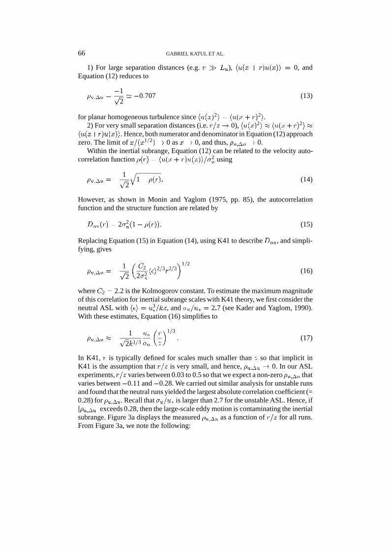
Figure 3e. The signature of ramp like patterns in the temperature time series for unstable (z=L =�0:32; upper figure) and near-neutral (z=L = �0:08; lower figure) atmospheric stability conditions.

��T;�u must vanish in order to derive (1). We use this correlation to measurelocal thermal effects on the longitudinal velocity inertial subrange eddy motion.Figure 3b displays ��T;�u as a function of r=z for up to 100. Notice that ��T;�uis not zero within the inertial subrange and a key assumption in the derivation ofthe Kolmogorov-Obukhov structure function equation is violated. Also, the factthat ��T;�u is finite further supports the conclusions by Antonia and Zhu (1994)regarding the role of temperature-velocity interactions and the anisotropy in thetemperature field. These conclusions were derived from the non-zero measuredvalues of the longitudinal heat flux co-spectrum.

4.3.3. Influence of Large Scale Thermals on the Small Scale Eddy MotionA measure of the net interaction between the large scale temperature field and thesmall scale longitudinal velocity is given by the correlation coefficient �T;�u

�T;�u(r) =h(T (x)� hT (x)i)(�u(x; r) � h�u(x; r)i)i

�T��u: (19)

The absence of any net interaction between the large scale temperature and smallscale velocity fluctuations requires �T;�u to be zero. If this correlation is finite, thenthe anisotropy characterizing the large scale thermal motion directly contributesto the small scale eddy motion of the longitudinal velocity. Hence, any interaction


Figure 3f. The temperature skewness derivative as a function of the Taylor microscale Reynoldsnumber. ST = 0:8 is from Sreenivasan et al. (1979) and the dotted line is from Sreenivasan (1991).

between T and �u indicates that local isotropy is not achieved. Figure 3c displays�T;�u as a function of r=z for dimensionless separation distances up to 100. Noticefrom Figure 3c that �T;�u is nearly zero within the inertial subrange and that large-scale thermal disturbances do not influence the local structure of the velocity field.This is qualitatively consistent with Figure 1a which shows that departures from3/4 do not depend on atmospheric stability conditions.

4.3.4. Influence of Large Scale Thermals on the Small Scale Thermal MotionIt was pointed out by Sreenivasan et al. (1979) that ramp-like structures directlycontribute to the inertial subrange of the temperature field without intermediate cas-cading steps, and therefore, may directly contribute to inertial subrange anisotropyin the Ta measurements. Such conclusions are in agreement with the ramp-likephenomenological model discussed by Van Atta (1977). If the ramp-like patternsare important to the anisotropy of the small-scale motion, then it is possible toevaluate this interaction from the correlation between T and �T using the samederivation as in u and �u. However, unlike the velocity field, it is difficult toestablish an upper limit for this interaction based on K41 since both the TKE and


Figure 3g. Same as Figure 3a but for �u;�T . For locally isotropic turbulence, �u;�T = 0.

the thermal dissipation rates are needed. For this purpose, a separate analysis forthe temperature field was developed and is summarized below:

(1) Expand the covariance hT�T 2i using

hT (x)[T (x+r)�T (x)]2i = hT (x)T (x+r)2i�2hT (x+r)T (x)2i+hT (x)3i(20)

and carry out the following simplifications by noting that:

(i) the mean temperature gradient skewness, defined as

ST (r) =jh(T (x + r)� T (x))3ij

(DTT (r))3=2; (21)

is zero for locally homogeneous and isotropic turbulence (Sreenivasan, 1991),so that

h[T (x+ r)� T (x)]3i = hT (x+ r)3i � 3hT (x+ r)2T (x)i+3hT (x+ r)T (x)2i+ hT (x)3i = 0; (22)

(ii) the third moment hT (x)3i is identical to hT (x+ r)3i for locally homogeneousturbulence so that Equation (21) reduces to

hT (x+ r)2T (x)i = hT (x)2T (x+ r)i; (23)


(2) use the identity in Equation (23) to simplify Equation (20). After severalalgebraic steps, Equation (20) reduces to

hT�T 2i = �hT 2�T i; (24)

and, hence, a dimensionless measure �(r) defined as

�(r) = �hT2�T i

hT�T 2i ; (25)

must be unity for locally isotropic turbulence. Notice that Equation (25) is definedby the ratio of two covariances: the covariance (hT�T 2i) measures the meaninfluence of large-scale temperature perturbations (T ) on the local thermal energy(�T 2) while the second covariance (hT 2�T i) measures the mean influence of localthermal perturbations (�T ) on large-scale thermal energy (T 2). As evidenced fromEquation (24), local isotropy requires a balance between these two covariances.Figure 3d shows the variation of �(r) for all runs. Notice in Figure 3d that �(r) issystematically less than unity suggesting that the interaction described by hT�T 2iis larger than the interaction described by hT 2�T i. Whether the departure of �(r)from unity is due to the ramp-like motion can be qualitatively assessed from Figures3e and 3d. The signatures of ramp-like patterns in the temperature time series forunstable (z=L = �0:32; upper figure) and near-neutral (z=L = �0:08; lowerfigure) conditions are shown in Figure 3e. It is evident that an apparent ramp-likesignature (upper figure) results in a stronger �(r) departure from unity (see Figure3d) when compared to the weak ramp-like signature (lower figure).

To further compare our measurements with other laboratory studies, especial-ly studies that considered the influence of ramp-like motion on the temperaturegradient skewness in the inertial subrange, we computed jST j and compared ourmeasurements with data from Gibson et al. (1977), Sreenivasan et al. (1979), andSreenivasan (1991) in Figure 3f. Recall that a zero jST j is central to �(r) = 1.Notice that the data in Figure 3f are not exclusively boundary-layer flows. TheTaylor microscale Reynolds number (Re = �u�=�) for many ASL flows are 3–10times larger than many laboratory boundary-layer flows. Recall that for a locallyisotropic temperature field, ST = 0. The ASL values in Figure 3f were obtained byaveraging the measured ST values between 0:1 < r=z < 0:2 and are summarizedin Table III. This range was chosen for all seven runs since i) DTT exhibits a2/3 power-law, ii) r > 3dsl and is well within the sonic anemometer temperatureresolution, and iii) r < 0.1 LT so that one decade of cascade steps have occured.Within this range, about 10 to 15 ST values were averaged. The ST = 0.8 constanttemperature skewness is from Gibson et al. (1977) and Sreenivasan et al. (1979),and the dashed line is an extrapolation from the data by Sreenivasan (1991). Noticein Figure 3f that ST is not zero for all runs (Run 4 was excluded from this compar-ison due to the large Iu) and that our ASL measurements are very comparable tothe heated boundary-layer laboratory data in Sreenivasan (1991).


4.3.5. Influence of Large Scale Velocity on the Small Scale Thermal MotionBased on the methodology previously proposed, this interaction can be character-ized by the correlation coefficient between u and �T so that,

��T;u(r) =h(u(x) � hu(x)i)(�T (x; r) � h�T (x; r)i)i

�u��T: (26)

Again, K41 and the Kolmogorov–Obukhov structure function for temperatureassume that this correlation is zero. In Figure 3g, ��T;u is displayed for all runs.From Figure 3g, note that ��T;u is nearly zero for separation distances up to 10z.Hence, Figure 3g suggests that the large scale velocity field and the small scalethermal disturbances are, to a first approximation, uncoupled within the inertialsubrange.

5. Conclusions

This study has examined the local structure of velocity and temperature close to theground surface. Despite the wide separation between production and dissipationlength scales, an inertial subrange, in the sense of Kolmogorov’s local isotropy,was not observed for the temperature field despite two decades of 2/3 power law inthe longitudinal velocity structure function. Departures from K41 scaling and localisotropy predictions where investigated for velocity and temperature by assumingthat the source of anisotropy is due to large scale–small scale interactions: Forquantifying such interactions, the following were considered:

[1] large scale–small scale velocity interactions.[2] local velocity–temperature interactions.[3] large scale temperature–local velocity interactions.[4] large scale temperature–local temperature interactions.[5] large scale velocity–local temperature interactions.

Special statistical measures were developed to quantify these interactions as afunction of scale (or separation distances). Here, we label and refer to the abovetypes of interactions as [1] to [5] respectively. Applying these statistical measuresto the temperature and velocity time series, the following conclusions were derived:

i) While the interactions described in [1], [3], [4], and [5] decrease with decreas-ing scale, the interaction in [2] appears to persist even at the smallest scalesresolved by the triaxial sonic anemometer. The zero interaction in [2] is anecessary condition for Obukhov’s (1949) hypothesis for the mixed velocitytemperature structure function.

ii) The temperature gradient skewness was measured and was found to be non-zero in agreement with many laboratory studies that included heated axisym-meteric wakes, heated two-dimensional wakes, and heated boundary layers.


Figure 4a. Comparison between triaxial sonic anemometer and thermocouple second order temper-ature structure function (DTT ) for hUi = 2:16 m s�1. The 2/3 power law is also shown. The sonicanemometer structure function is shifted upward one decade to permit comparison at small separationdistances.

The consequence of the non-zero temperature gradient skewness was furtherformulated in terms of an imbalance between two covariances that measure theinteraction between the local thermal energy and the large-scale temperatureperturbation, and the large-scale thermal energy and the local thermal pertur-bation. It was shown that for a locally isotropic temperature field, these twocovariances must be identical. Our measurements showed that the interactionbetween the local thermal energy and the large-scale temperature perturba-tion is systematically larger than the large-scale thermal energy–local thermalperturbation interaction.

iii) The fact that the local velocity and thermal eddy motion interact at the smallscales also suggests that local isotropy in the temperature field may not be fullyattained close to the ground surface despite the presence of a 2/3 power law inthe longitudinal velocity structure function. This finite interaction is in agree-ment with recent measurements by Antonia and Zhu (1994). However, it wasalso shown that such interactions result in minor departures from Obukhov’s(1949) hypothesis for the mixed velocity-temperature structure function.


Figure 4b. Same as Figure 4a but for hUi = 1:18 m s�1.

iv) The interaction in [5] decays very rapidly with decreasing scale suggestingrapid decoupling between the local thermal disturbances and the larger-scaleeddy motion. Our analysis does suggest that the local structure of the temper-ature field is, to a first approximation, uncoupled from the large scale energycontaining eddy motion.

v) While the linear ramp model suggested by Antonia and Van Atta (1978),Antonia et al. (1982) and Antonia and Chambers (1978) does address the non-zero values in odd-ordered temperature structure functions, it does not accountfor any interactions with the local velocity field. Refined ramp models shouldconsider this potential interaction.

vi) Finally, this study clearly demonstrates that K41 power laws derived fromstructure function measurements are not very sensitive to the isotropic state ofturbulence despite the fact that local isotropy is central to the derivation of thesepower laws. Our study suggested that local isotropy is not strictly achievedeven at scales comparable to z/2, but the longitudinal velocity structure func-tion does exhibit a clear 2/3 power law for scales comparable to 5z. Also,despite a non-zero structure skewness, the second-order temperature structure


function exhibits a near 2/3 power law and the normalized velocity-temperaturestructure function approximately follows Obukhov’s (1949) hypothesis.

Acknowledgements

The authors would like to thank Judd Edeburn for his help and support at theDuke Forest and the two reviewers for their helpful comments. Also, the authorsgreatly appreciate the suggested analysis from one of the anonymous referees forSection 4.3. This project was funded, in part, by the Environmental ProtectionAgency (EPA) under the co-operative agreement 91-0074-94 (CR817766), and theNational Science Foundation (NSF-BIR12333).

Appendix A:Comparison between Triaxial Sonic Anemometer and Thermocouple

Temperature Fluctuations

In this appendix, an assessment on how well the Gill triaxial sonic anemometermeasures the temperature fluctuations from the fluctuations in the speed of soundis carried out. For that purpose, three Campbell Scientific fine wire thermocouples(diameter = 0.013 mm, expected frequency response 5–10 Hz), situated at z = 2.6m are compared to the triaxial sonic anemometer at z = 2.75 m from an experimentcarried out in October, 1994 at the same grass clearing. The three thermocoupleswere situated on a horizontal rod, 1.8 m in length, with two thermocouples on thesides (East–West) of the rod and one thermocouple at the center. The triaxial sonicanemometer was situated 15 cm above the westerly thermocouple.

The data were sampled at 10 Hz for 27.3 minutes (N= 16,384 data points)using a 21X Campbell Scientific micrologger and transferred to a 486 Gatewaypersonal computer using an isolated optical interface. The analog output from theGill sonic anemometer was logged, (which is not of the same quality as the digitaldata) and the temperature was computed from Equation (4). In Figures 4a and 4b,the temperature structure functions of all four instruments are compared for hUi= 2.16 m s�1, and hUi = 1.18 m s�1, respectively. The Gill temperature structurefunction measurements are shifted by one decade to permit comparisons for smallseparation distances. The separation distance was computed from time incrementsusing Taylor’s (1938) frozen turbulence hypothesis and the mean horizontal windspeed from the sonic anemometer. These two sample runs were chosen becausethe wind direction was from the north minimizing mast and other instrumentinterferences. The 2/3 power-law is also shown. Notice in Figure 4b that beyondr = dsl, the volume averaging by the finite sonic path artificially creates additionaldissipation resulting in structure function power-laws much steeper than 2/3. Forr > dsl, good agreement between the sonic anemometer temperature measurements


and the fine wire thermocouple is noted, in agreement with an earlier comparisonby Katul (1994).

References

Antonia, R. A. and Van Atta, C. W.: 1975, ‘On the Correlation between Temperature and VelocityDissipation Fields in a Heated Turbulent Jet’, J. Fluid Mech. 67, 273–287.

Antonia, R. A. and Van Atta, C. W.: 1978, ‘Structure Functions of Temperature Fluctuations inTurbulent Shear Flows’, J. Fluid Mech. 84, 561–580.

Antonia, R. A. and Chambers, A. J.: 1978, ‘Note on the Temperature Ramp Structure in the MarineSurface Layer’, Boundary-Layer Meteorol. 15, 347–355.

Antonia, R. A., Chambers, A. J., Friehe, C. A., and Van Atta, C. W.: 1979, ‘Temperature Ramps inthe Atmospheric Surface Layer’, J. Atmos. Sci. 36, 99–108.

Antonia, R. A. and Chambers, A. J.: 1980, ‘On the Correlation between Turbulent Velocity andTemperature Derivatives in the Atmospheric Surface Layer’, Boundary-Layer Meteorol. 18, 399-410.

Antonia, R. A., Chambers, A. J., and Bradley, E. F.: 1982, ‘Relationship Between Structure Functionsand Temperature Ramps in the Atmospheric Surface Layer’, Boundary-Layer Meteorol. 23,395–403.

Antonia, R. A., Anselmet, F., and Chambers, A. J.: 1984, ‘Assessment of Local Isotropy UsingMeasurements in a Turbulent Plane Jet’, J. Fluid Mech. 163, 365–390.

Antonia, R. A., and Kim, J.: 1994, ‘A Numerical Study of Local Isotropy of Turbulence’,Phys. Fluids6, 834–841.

Antonia, R. A., and Zhu, Y.: 1994, ‘Inertial Range Behavior of the Longitudinal Heat Flux Cospec-trum’, Boundary-Layer Meteorol. 70, 429–434.

Busch, N.: 1973, ‘The Surface Boundary Layer, Part I’, Boundary-Layer Meteorol. 4, 213–240.Bradley, E. F., Antonia, R. A., Chambers, A. J.: 1981, ‘Turbulence Reynolds Number and the Turbulent

Kinetic Energy Balance in the Atmospheric Surface Layer’, Boundary-Layer Meteorol. 21, 183–197.

Brutsaert, W.: 1982, Evaporation into the Atmosphere: Theory, History, and Applications, KluwerAcademic Publishers, 299 pp.

Fisher, M. J. and Davies, P. O. A.: 1964, ‘Correlation Measurements in a Non-Frozen PatternTurbulence’, J. Fluid Mech. 18, 97–116.

Frisch, U., Sulem, P., and Nelkin, M.: 1978, ‘A Simple Dynamical Model of Intermittent FullyDeveloped Turbulence’, J. Fluid Mech. 87, 719–736.

Gibson, C. H., Friehe, C. A., and McConnell, S. O.: 1977, ‘Structure of Sheared Turbulent Fields’,Phys. Fluids 20, s156–167.

Gibson, C. H., Ashurst, W. T., and Kerstein, A. R.: 1988, ‘Mixing of Strongly Diffusive PassiveScalars Like Temperature by Turbulence’, J. Fluid Mech. 194, 261–293.

Kader, B. A., Yaglom, A. M., and Zubkovskii, S. L.: 1989, ‘Spatial Correlation Functions of Surface-Layer Turbulence in Neutral Stratification’, Boundary-Layer Meteorol. 47, 233–249.

Kaimal, J. C., Wyngaard, J. C., Izumi, Y., and Cote, O. R.: 1972, ‘Spectral Characteristics of SurfaceLayer Turbulence’, Quart. J. Roy. Meteorol. Soc. 98, 563–589.

Kaimal, J. C.: 1986, ‘Flux and Profile Measurements from Towers in the Boundary Layer’, in D.H. Lenschow (ed.), Probing the Atmospheric Boundary Layer, American Meterological Society,Boston, Massachusetts, pp. 19–28.

Kaimal, J. C., and Finnigan, J. J.: 1994, Atmospheric Boundary Layer Flows: Their Structure andMeasurements, Oxford, 289 pp.

Katul, G. G., Parlange, M. B., and Chu, C. R.: 1994a, ‘Intermittency, Local Isotropy, and Non-Gaussian Statistics in Atmospheric Surface Layer Turbulence’, Physics of Fluids 7, 2480–2492.

Katul, G. G.: 1994, ‘A Model for Sensible Heat Flux Probability Density Function for Near-Neutraland Slightly-Stable Atmospheric Flows’, Boundary-Layer Meteorol. 71, 1–20.


Katul, G. G., Albertson, J. D., Chu, C. R., and Parlange, M. B.: 1994b, ‘Intermittency in AtmosphericSurface Layer Turbulence: The Orthonormal Wavelet Representation’, in E. Foufoula-Georgiouand P. Kumar (eds.), in Wavelets in Geophysics, Academic Press, 365 pp.

Katul, G. G., Parlange, M. B., Albertson, J. D., and Chu, C. R.: 1995a, ‘Local Isotropy and Anisotropyin the Sheared and Heated Atmospheric Surface Layer, Boundary-Layer Meteorol. 72, 123–148.

Katul, G. G., Parlange, M. B., Albertson, J. D., and Chu, C. R.: 1995b, ‘The Random SweepingDecorrelation Hypothesis in Stratified Turbulent Flows’, Fluid Dyn. Res. 16, 275–295.

Kerr, R. M.: 1985, ‘Higher-Order Derivative Correlations and the Alignment of Small-Scale Structuresin Isotropic Numerical Turbulence’, J. Fluid Mech. 153, 31–58.

Kerr, R. M.: 1990, ‘Velocity, Scalar, and Transfer Spectra in Numerical Turbulence’, J. Fluid Mech.211, 309–332.

Kolmogorov, A. N.: 1941, ‘The Local Structure of Turbulence in Incompressible Viscous Fluid forVery Large Reynolds Number’, Dokl. Akad. Nauk. SSSR, 30, 301–303.

Kolmogorov, A. N.: 1962, ‘A Refinement of Previous Hypotheses Concerning the Local Structureof Turbulence in a Viscous Incompressible Fluid at High Reynolds Number’, J. Fluid Mech. 13,82–85.

Kuznetsov, V. R., Praskovsky, A. A., and Sabelnikov, V. A.: 1992, ‘Fine-Scale Turbulence Structureof Intermittent Shear Flows’, J. Fluid Mech. 243, 595–622.

Landau, L. D., and Lifshitz, E. M.: 1986, Fluid Mechanics, Pergamon Press, 539 pp.Jayesh, C. Tong, and Warhaft, Z.: 1994, ‘On Temperature Spectra in Grid Turbulence’, Phys. Fluids

6, 306–312.Lin, C. C.: 1953, ‘On Taylor’s Hypothesis and the Acceleration Terms in the Navier-Stokes Equations’,

Q. Appl. Math. X, 154–165.Lumley, J. and Panofsky, H.: 1964, The Structure of Atmospheric Turbulence, John Wiley and Sons,

229 pp.Lumley, J. L.: 1965, ‘Interpretation of Time Spectra Measured in High-Intensity Shear Flows’, Phys.

Fluids 8, 1056–1062.Mahrt, L.: 1989, ‘Intermittency of Atmospheric Turbulence’, J. Atmos. Sci. 46, 79–95.Mestayer, P.: 1982, ‘Local Isotropy and Anisotropy in a High Reynolds Number Turbulent Boundary

Layer’, J. Fluid Mech. 125, 475–503.Mizuno, T. and Panofsky, H. A.: 1975, ‘The Validity of Taylor’s Hypothesis in the Atmospheric

Surface Layer’, Boundary-Layer Meteorol. 9, 375–380.Monin, A. S. and Yaglom, A. M.: 1971, Statistical Fluid Mechanics, Vol. I., MIT Press, 769 pp.Monin, A. S. and Yaglom, A. M.: 1975, Statistical Fluid Mechanics, Vol. II, MIT Press, 875 pp.Obukhov, A. M.: 1949, ‘Local Structure of Atmospheric Turbulence’, Dokl. Akad. Nauk. SSSR 67,

643–646.Panofsky, H. and Dutton, J.: 1984, Atmospheric Turbulence: Models and Methods for Engineering

Applications, John Wiley and Sons, 397 pp.Pond, S., Stewart, R. W., and Burling, R. W.: 1963, ‘Turbulence Spectra in the Wind Over Waves’, J.

Atmos. Sci. 20, 319–324.Powell, D. C. and Elderkin, C. E.: 1974, ‘An Investigation of the Application of Taylor’s Frozen

Hypothesis to Atmospheric Boundary Layer Turbulence’, J. Atmos. Sci. 31, 990–1002.Praskovsky, A. A., Gledzer, E. B., Karyakin, M. Y., and Zhou, Y.: 1993, ‘The Sweeping Decorrelation

Hypothesis and Energy-Inertial Scale Interaction in High Reynolds Number Flows’, J. FluidMech. 248, 493–511.

Saddoughi, S. G. and Veeravalli, S. V.: 1994, ‘Local Isotropy in Turbulent Boundary Layers at HighReynolds Number’, J. Fluid Mech. 268, 333–372.

Sirivat, A. and Warhaft, Z.: 1983, ‘The Effect of a Passive Cross-Stream Temperature Gradient onthe Evolution of Temperature Variance and Heat Flux in Grid Turbulence’, J. Fluid Mech. 128,323–346.

Sreenivasan, K. R., Antonia, R. A., and Britz, D.: 1979, ‘Local Isotropy and Large Structures in aHeated Turbulent Jet’, J. Fluid Mech. 94, 745–775.

Sreenivasan, K. R.: 1991, ‘On Local Isotropy of Passive Scalars in Turbulent Shear Flows’, in J. C. R.Hunt, O. M. Phillips and D. Williams (eds.), Turbulence and Stochastic Processes: Kolmogorov’sIdeas 50 Years On, Roy. Soc. 240 pp.


Stull, R.: 1988, An Introduction to Boundary Layer Meteorology, Kluwer Academic Publishers, 666pp.

Taylor, G. I.: 1938, ‘The Spectrum of Turbulence’, Proc. Roy. Soc. A 1164, 476–490.Tennekes, H. and Lumley, J. L.: 1972, A First Course in Turbulence, MIT Press, 300 pp.Townsend, A. A.: 1976, The Structure of Turbulent Shear Flow, Cambridge University Press, 429 pp.Van Atta, C. W.: 1977, ‘Effect of Coherent Structures on the Structure Functions of Temperature in

the Atmospheric Boundary Layer’, Arch. Mech. 29, 161–171.Wyngaard, J. C. and Clifford, S. F.: 1977, ‘Taylor’s Hypothesis and High Frequency Turbulence

Spectra’, J. Atmos. Sci. 34, 922–929.Wyngaard, J. C.: 1981, ‘Cup, Propeller, Vane, and Sonic Anemometer in Turbulence Research’, Ann.

Rev. Fluid Mech. 13, 922–929.

gabriel katul, cheng-i hsieh and john sigmon50 gabriel katul et al. and x 3(= z) are the...

Documents