fundamentals grady notes june 2007 print
TRANSCRIPT
7/22/2019 Fundamentals Grady Notes June 2007 Print
http://slidepdf.com/reader/full/fundamentals-grady-notes-june-2007-print 1/388
Table of Contents
1. Fundamentals p. 2
2. Three Phase Circuits p. 40
3. Transformers p. 56
4. Per Unit System and Sequence Networks p. 86
5. Transmission Lines p. 115
6. Symmetrical Components p. 165
7. More Sequence Networks p. 1718. System Matrices p. 175
9. Programming Considerations p. 213
10. Short Circuits and Voltage Sags p. 228
11. Loadflow p. 270
12. Stability p. 314
13. Lightning, Grounding, and Shock Energy p. 338
14. Harmonic Filters p. 386
Fundamentals of Electric Power Systems
Prof. Mack Grady
Dept. of Electrical & Computer Engineering
University of Texas at [email protected], www.ece.utexas.edu/~grady
June 2007
Grady 2007, p. 1
7/22/2019 Fundamentals Grady Notes June 2007 Print
http://slidepdf.com/reader/full/fundamentals-grady-notes-june-2007-print 2/388
M a g =
1 0
1 2
8
A n g =
0
- 9 0
4 5
- 3 6 0
1 0
3 . 6
8 E - 1
5
5 . 6
5 6 8 5 4
1 5
. 6 5 6 8 5
- 3 5 8
9 . 9
9 3 9 0 8
0 . 4
1 8 7 9 4
5 . 4
5 5 9 8 7
1 5
. 8 6 8 6 9
- 3 5 6
9 . 9
7 5 6 4 1
0 . 8
3 7 0 7 8
5 . 2
4 8 4 7 2
1 6
. 0 6 1 1 9
- 3 5 4
9 . 9
4 5 2 1 9
1 . 2
5 4 3 4 2
5 . 0
3 4 5 6 3
1 6
. 2 3 4 1 2
- 3 5 2
9 . 9
0 2 6 8 1
1 . 6
7 0 0 7 7
4 . 8
1 4 5 2
1 6
. 3 8 7 2 8
- 3 5 0
9 . 8
4 8 0 7 8
2 . 0
8 3 7 7 8
4 . 5
8 8 6 1 1
1 6
. 5 2 0 4 7
- 3 4 8
9 . 7
8 1 4 7 6
2 . 4
9 4 9 4
4 . 3
5 7 1 1 2
1 6
. 6 3 3 5 3
- 3 4 6
9 . 7
0 2 9 5 7
2 . 9
0 3 0 6 3
4 . 1
2 0 3 0 5
1 6
. 7 2 6 3 2
- 3 4 4
9 . 6
1 2 6 1 7
3 . 3
0 7 6 4 8
3 . 8
7 8 4 7 7
1 6
. 7 9 8 7 4
- 3 4 2
9 . 5
1 0 5 6 5
3 . 7
0 8 2 0 4
3 . 6
3 1 9 2 4
1 6
. 8 5 0 6 9
- 3 4 0
9 . 3
9 6 9 2 6
4 . 1
0 4 2 4 2
3 . 3
8 0 9 4 6
1 6
. 8 8 2 1 1
- 3 3 8
9 . 2
7 1 8 3 9
4 . 4
9 5 2 7 9
3 . 1
2 5 8 4 9
1 6
. 8 9 2 9 7
- 3 3 6
9 . 1
3 5 4 5 5
4 . 8
8 0 8 4
2 . 8
6 6 9 4 4
1 6
. 8 8 3 2 4
- 3 3 4
8 . 9
8 7 9 4
5 . 2
6 0 4 5 4
2 . 6
0 4 5 4 5
1 6
. 8 5 2 9 4
- 3 3 2
8 . 8
2 9 4 7 6
5 . 6
3 3 6 5 9
2 . 3
3 8 9 7 4
1 6
. 8 0 2 1 1
- 3 3 0
8 . 6
6 0 2 5 4
6
2 . 0
7 0 5 5 2
1 6
. 7 3 0 8 1
- 3 2 8
8 . 4
8 0 4 8 1
6 . 3
5 9 0 3 1
1 . 7
9 9 6 0 8
1 6
. 6 3 9 1 2
- 3 2 6
8 . 2
9 0 3 7 6
6 . 7
1 0 3 1 5
1 . 5
2 6 4 7 2
1 6
. 5 2 7 1 6
- 3 2 4
8 . 0
9 0 1 7
7 . 0
5 3 4 2 3
1 . 2
5 1 4 7 6
1 6
. 3 9 5 0 7
- 3 2 2
7 . 8
8 0 1 0 8
7 . 3
8 7 9 3 8
0 . 9
7 4 9 5 5
1 6
. 2 4 3
- 3 2 0
7 . 6
6 0 4 4 4
7 . 7
1 3 4 5 1
0 . 6
9 7 2 4 6
1 6
. 0 7 1 1 4
- 3 1 8
7 . 4
3 1 4 4 8
8 . 0
2 9 5 6 7
0 . 4
1 8 6 8 8
1 5
. 8 7 9 7
- 3 1 6
7 . 1
9 3 3 9 8
8 . 3
3 5 9
0 . 1
3 9 6 1 9
1 5
. 6 6 8 9 2
- 3 1 4
6 . 9
4 6 5 8 4
8 . 6
3 2 0 7 8
- 0 . 1
3 9 6 2
1 5
. 4 3 9 0 4
- 3 1 2
6 . 6
9 1 3 0 6
8 . 9
1 7 7 3 8
- 0 . 4
1 8 6 9
1 5
. 1 9 0 3 6
- 3 1 0
6 . 4
2 7 8 7 6
9 . 1
9 2 5 3 3
- 0 . 6
9 7 2 5
1 4
. 9 2 3 1 6
- 3 0 8
6 . 1
5 6 6 1 5
9 . 4
5 6 1 2 9
- 0 . 9
7 4 9 5
1 4
. 6 3 7 7 9
- 3 0 6
5 . 8
7 7 8 5 3
9 . 7
0 8 2 0 4
- 1 . 2
5 1 4 8
1 4
. 3 3 4 5 8
- 3 0 4
5 . 5
9 1 9 2 9
9 . 9
4 8 4 5 1
- 1 . 5
2 6 4 7
1 4
. 0 1 3 9 1
- 3 0 2
5 . 2
9 9 1 9 3
1 0
. 1 7 6 5 8
- 1 . 7
9 9 6 1
1 3
. 6 7 6 1 6
- 3 0 0
5
1 0
. 3 9 2 3
- 2 . 0
7 0 5 5
1 3
. 3 2 1 7 5
- 2 9 8
4 . 6
9 4 7 1 6
1 0
. 5 9 5 3 7
- 2 . 3
3 8 9 7
1 2
. 9 5 1 1 1
- 2 9 6
4 . 3
8 3 7 1 1
1 0
. 7 8 5 5 3
- 2 . 6
0 4 5 5
1 2
. 5 6 4 6 9
- 2 9 4
4 . 0
6 7 3 6 6
1 0
. 9 6 2 5 5
- 2 . 8
6 6 9 4
1 2
. 1 6 2 9 7
- 2 9 2
3 . 7
4 6 0 6 6
1 1
. 1 2 6 2 1
- 3 . 1
2 5 8 5
1 1
. 7 4 6 4 2
- 2 9 0
3 . 4
2 0 2 0 1
1 1
. 2 7 6 3 1
- 3 . 3
8 0 9 5
1 1
. 3 1 5 5 7
- 2 8 8
3 . 0
9 0 1 7
1 1
. 4 1 2 6 8
- 3 . 6
3 1 9 2
1 0
. 8 7 0 9 2
- 2 8 6
2 . 7
5 6 3 7 4
1 1
. 5 3 5 1 4
- 3 . 8
7 8 4 8
1 0
. 4 1 3 0 4
- 2 8 4
2 . 4
1 9 2 1 9
1 1
. 6 4 3 5 5
- 4 . 1
2 0 3
9 . 9
4 2 4 6 3
- 2 8 2
2 . 0
7 9 1 1 7
1 1
. 7 3 7 7 7
- 4 . 3
5 7 1 1
9 . 4
5 9 7 7 6
- 2 8 0
1 . 7
3 6 4 8 2
1 1
. 8 1 7 6 9
- 4 . 5
8 8 6 1
8 . 9
6 5 5 6 3
- 2 7 8
1 . 3
9 1 7 3 1
1 1
. 8 8 3 2 2
- 4 . 8
1 4 5 2
8 . 4
6 0 4 2 8
- 2 7 6
1 . 0
4 5 2 8 5
1 1
. 9 3 4 2 6
- 5 . 0
3 4 5 6
7 . 9
4 4 9 8 4
- 2 7 4
0 . 6
9 7 5 6 5
1 1
. 9 7 0 7 7
- 5 . 2
4 8 4 7
7 . 4
1 9 8 6 1
- 3 0
- 2 0
- 1 0 0
1 0
2 0
3 0
- 3 6 0
- 2 7 0
- 1 8 0
- 9 0
0
9 0
1 8 0
2 7 0
3 6 0
- 3 0
- 2 0
- 1 0 0
1 0
2 0
3 0
- 3 6 0
- 2 7 0
- 1 8 0
- 9 0
0
9 0
1 8 0
2 7 0
3 6 0
Grady 2007, p. 2
7/22/2019 Fundamentals Grady Notes June 2007 Print
http://slidepdf.com/reader/full/fundamentals-grady-notes-june-2007-print 3/388
Grady 2007, p. 3
7/22/2019 Fundamentals Grady Notes June 2007 Print
http://slidepdf.com/reader/full/fundamentals-grady-notes-june-2007-print 4/388
Grady 2007, p. 4

7/22/2019 Fundamentals Grady Notes June 2007 Print
http://slidepdf.com/reader/full/fundamentals-grady-notes-june-2007-print 5/388
Grady 2007, p. 5

7/22/2019 Fundamentals Grady Notes June 2007 Print
http://slidepdf.com/reader/full/fundamentals-grady-notes-june-2007-print 6/388
Grady 2007, p. 6
7/22/2019 Fundamentals Grady Notes June 2007 Print
http://slidepdf.com/reader/full/fundamentals-grady-notes-june-2007-print 7/388
Grady 2007, p. 7
7/22/2019 Fundamentals Grady Notes June 2007 Print
http://slidepdf.com/reader/full/fundamentals-grady-notes-june-2007-print 8/388
Grady 2007, p. 8
7/22/2019 Fundamentals Grady Notes June 2007 Print
http://slidepdf.com/reader/full/fundamentals-grady-notes-june-2007-print 9/388
Grady 2007, p. 9

7/22/2019 Fundamentals Grady Notes June 2007 Print
http://slidepdf.com/reader/full/fundamentals-grady-notes-june-2007-print 10/388
Grady 2007, p. 10

7/22/2019 Fundamentals Grady Notes June 2007 Print
http://slidepdf.com/reader/full/fundamentals-grady-notes-june-2007-print 11/388
Grady 2007, p. 11

7/22/2019 Fundamentals Grady Notes June 2007 Print
http://slidepdf.com/reader/full/fundamentals-grady-notes-june-2007-print 12/388
Grady, Definitions, June 2007, Page 1
Definitions
Definitions related to power. RMS values, active and reactive power, power factor, power flow
in transmission lines. Review of per unit system and the advantages that it offers.
1. Single-Phase Definitions
The root-mean-squared (RMS) value of a periodic voltage (or current) waveform is
T ot
ot
RMS dt t vT
V )(1 2
, where T is the period of v(t).
If )sin()( t V t v , where V is the peak value, then using2
)2cos(1)(sin 2 A
A
, RMS V
becomes
2
V V RMS .
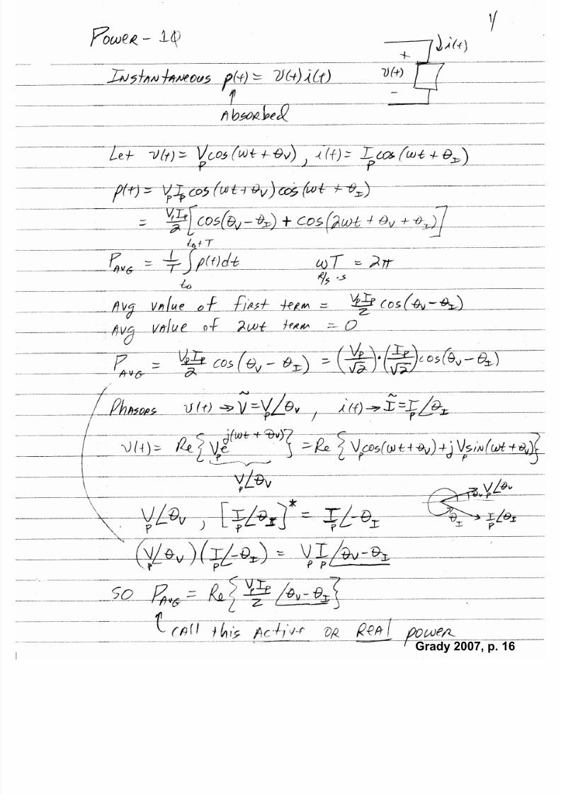
Instantaneous power flowing to a load, using the sign convention shown in Figure 1, is defined
as
)()()( t it vt p .
v(t)
i(t)
+
-
p(t) = v(t) i(t)
--->
---> p(t)
Figure 1. Instantaneous Power Flowing Into a Load
Average power flowing to a load is defined as
T ot
ot
dt t p
T
P )(1
, where T is the period of )(t p .
If )sin()( t V t v , )sin()( t I t i , then the instantaneous power becomes
)2cos()cos(2
)()()( t VI
t it vt p .
Grady 2007, p. 12
7/22/2019 Fundamentals Grady Notes June 2007 Print
http://slidepdf.com/reader/full/fundamentals-grady-notes-june-2007-print 13/388
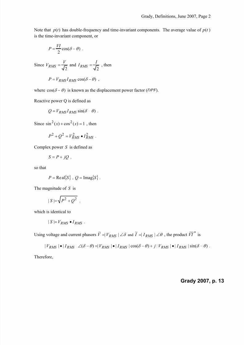
Grady, Definitions, June 2007, Page 2
Note that )(t p has double-frequency and time-invariant components. The average value of )(t p
is the time-invariant component, or
)cos(2
VI
P .
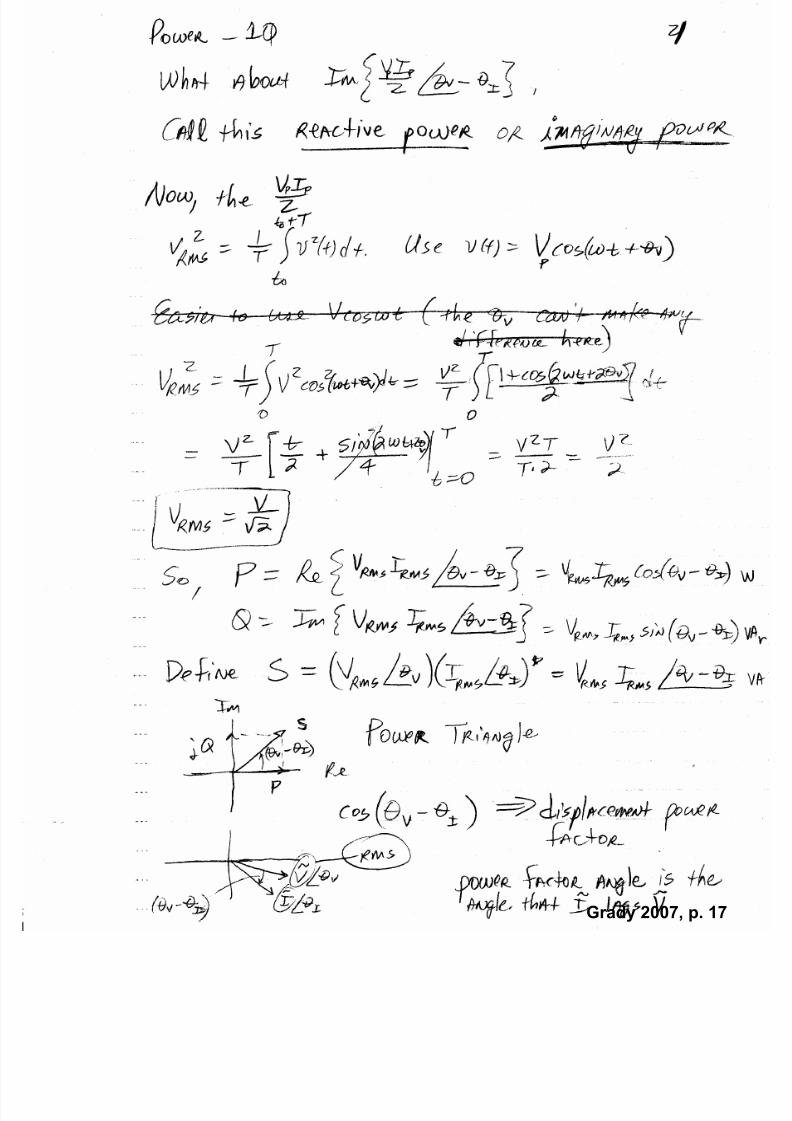
Since2
V V RMS and
2
I I RMS , then
)cos( RMS RMS I V P ,
where )cos( is known as the displacement power factor ( DPF ).
Reactive power Q is defined as
)sin( RMS RMS I V Q .
Since 1)(cos)(sin 22 x x , then
2222 RMS RMS I V Q P .
Complex power S is defined as
jQ P S ,
so that
S P alRe , S Q Imag .
The magnitude of S is
22|| Q P S ,
which is identical to
RMS RMS I V S || .
Using voltage and current phasors ||~
RMS V V and ||~
RMS I I , the product *~~ I V is
)sin(||||)cos(||||)(|||| RMS RMS RMS RMS RMS RMS I V j I V I V .
Therefore,
Grady 2007, p. 13
7/22/2019 Fundamentals Grady Notes June 2007 Print
http://slidepdf.com/reader/full/fundamentals-grady-notes-june-2007-print 14/388
Grady, Definitions, June 2007, Page 3
*~~ I V jQ P S .
When I ~
lags V ~
, Q is positive, and the power factor is lagging. When I ~
leads V ~
, Q is
negative, and the power factor is leading. Thus, an inductive load has a lagging power factor and
absorbs Q, while a capacitive load has a leading power factor and produces Q.
The total power factor DPF is defined as
S
P DPF .
For sinusoidal systems, total power factor is identical to displacement power factor defined
previously as the cosine of the relative phase angle between voltage and current.
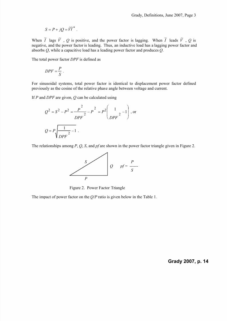
If P and DPF are given, Q can be calculated using
11
2
22
2
2222
DPF
P P
DPF
P P S Q , or
11
2
DPF
P Q .
The relationships among P , Q, S , and pf are shown in the power factor triangle given in Figure 2.
P
QS
pf = ------ P
S
Figure 2. Power Factor Triangle
The impact of power factor on the Q/P ratio is given below in the Table 1.
Grady 2007, p. 14

7/22/2019 Fundamentals Grady Notes June 2007 Print
http://slidepdf.com/reader/full/fundamentals-grady-notes-june-2007-print 15/388
Grady, Definitions, June 2007, Page 4
DPF Q / P
1.0 0.00
0.9 0.48
0.8 0.75
0.707 1.00
0.6 1.33
Table 1. Impact of Power Factor on Reactive Power Q
Now, consider the power flow through a purely inductive circuit element, such as a lossless
transmission line or transformer shown in Figure 3.
j X
+
-
+
-
P + j Q -->
Vs Vr r s
Figure 3. Power Flow Through a Purely Inductive Circuit Element
The active and reactive power flows, measured at the sending end S, can be shown to be
)sin( RS RS
X
V V P , )cos( RS RS
S V V X
V Q .
Usually, )( RS is small, so that
)( RS P , RS S V V
X
V Q .
Therefore, in inductive circuit elements, P tends to be proportional to voltage angle difference,
and Q tends to be proportional to voltage magnitude difference.
Grady 2007, p. 15
7/22/2019 Fundamentals Grady Notes June 2007 Print
http://slidepdf.com/reader/full/fundamentals-grady-notes-june-2007-print 16/388
Grady 2007, p. 16
7/22/2019 Fundamentals Grady Notes June 2007 Print
http://slidepdf.com/reader/full/fundamentals-grady-notes-june-2007-print 17/388
Grady 2007, p. 17

7/22/2019 Fundamentals Grady Notes June 2007 Print
http://slidepdf.com/reader/full/fundamentals-grady-notes-june-2007-print 18/388
Grady 2007, p. 18

7/22/2019 Fundamentals Grady Notes June 2007 Print
http://slidepdf.com/reader/full/fundamentals-grady-notes-june-2007-print 19/388
Grady 2007, p. 19
7/22/2019 Fundamentals Grady Notes June 2007 Print
http://slidepdf.com/reader/full/fundamentals-grady-notes-june-2007-print 20/388
Grady 2007, p. 20

7/22/2019 Fundamentals Grady Notes June 2007 Print
http://slidepdf.com/reader/full/fundamentals-grady-notes-june-2007-print 21/388
Grady 2007, p. 21

7/22/2019 Fundamentals Grady Notes June 2007 Print
http://slidepdf.com/reader/full/fundamentals-grady-notes-june-2007-print 22/388
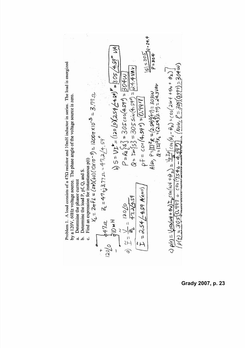
A load consists of a 47 resistor and 10mH inductor in series. The load is energized by a 120V,
60Hz voltage source. The phase angle of the voltage source is zero.a. Determine the phasor current
b. Determine the load P, pf, Q, and S.
c. Find an expression for instantaneous p(t)
Grady 2007, p. 22
7/22/2019 Fundamentals Grady Notes June 2007 Print
http://slidepdf.com/reader/full/fundamentals-grady-notes-june-2007-print 23/388
Grady 2007, p. 23

7/22/2019 Fundamentals Grady Notes June 2007 Print
http://slidepdf.com/reader/full/fundamentals-grady-notes-june-2007-print 24/388
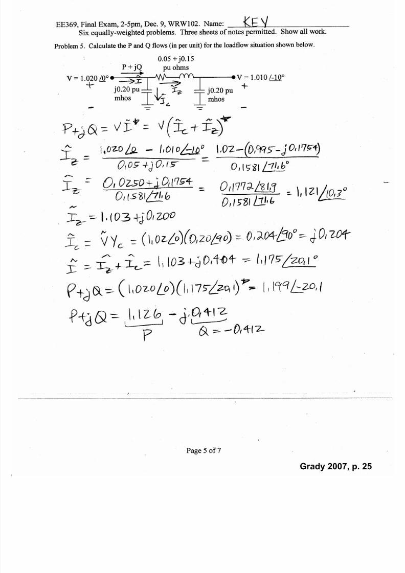
Calculate the P and Q flows (in per unit) for the loadflow situation shown below.
0.05 + j0.15
pu ohms
j0.20 pumhos
j0.20 pumhos
P + jQ
V = 1.020 /0° V = 1.010 /-10°
Grady 2007, p. 24
7/22/2019 Fundamentals Grady Notes June 2007 Print
http://slidepdf.com/reader/full/fundamentals-grady-notes-june-2007-print 25/388
Grady 2007, p. 25

7/22/2019 Fundamentals Grady Notes June 2007 Print
http://slidepdf.com/reader/full/fundamentals-grady-notes-june-2007-print 26/388
Notes on Nodal Analysis
Definitions
Node: A point or set of points at the same potential that have at least two branches
connected to them.
Branch: A circuit element that connects nodes.
Major Node: A node with three or more branches connected to it.
Super Node: Two major nodes with an ideal voltage source between them.
Reference Node: The node to which all other node potentials are referenced. The relativevoltage of the reference node is zero.
Solution Procedure
1. Draw a neat circuit diagram and try to eliminate as many branch crossings as possible.
2. Choose a reference node. All other node voltages will be referenced to it. Ideally, it
should be the node with the most branches connected to it, so that the number of terms in
the admittance matrix is minimal.
3. If the circuit contains voltage sources, do either of the following:
Convert them to current sources (if they have series impedances)
Create super nodes by encircling the corresponding end nodes of each voltage source.
4. Assign a number to every major node (except the reference node) that is not part of asuper node (N1 of these).
5. Assign a number to either end (but not both ends) of every super node that does not touch
the reference node (N2 of these)
6. Apply KCL to every numbered node from Step 4 (N1 equations)
7. Apply KCL to every numbered super node from Step 5 (N2 equations)
8. The dimension of the problem is now N1 + N2. Solve the set of linear equations for the
node voltages. At this point, the circuit has been “solved.”
9. Using your results, check KCL for at least one node to make sure that your currents sum
to zero.
9. Use Ohm’s Law, KCL, and the voltage divider principle to find other node voltages,
branch currents, and powers as needed.
Grady 2007, p. 26
7/22/2019 Fundamentals Grady Notes June 2007 Print
http://slidepdf.com/reader/full/fundamentals-grady-notes-june-2007-print 27/388
Notes on Mesh Analysis
Definitions
Branch: A circuit element that connects nodes
Planar Network: A network whose circuit diagram can be drawn on a plane in such a
manner that no branches pass over or under other branches
Loop: A closed path
Mesh: A loop that is the only loop passing through at least one branch
Solution Procedure
1. Draw a neat circuit diagram and make sure that the circuit is planar (if not
planar, then the circuit is not a candidate for mesh analysis)
2. If the circuit contains current sources, do either of the following:
A. Convert them to voltage sources (if they have internal impedances), or
B. Create super meshes by making sure in Step 3 that two (and not more than
two) meshes pass through each current source. SM super meshes.
3. Draw clockwise mesh currents, where each one passes through at least one
new branch. M meshes.
4. Apply KVL for every mesh that is not part of a super mesh (M – 2SM
equations)
5. For meshes that form super meshes, apply KVL to the portion of the loop
formed by the two meshes that does not pass through the current source (SMequations)
6. For each super mesh, write an equation that relates the corresponding meshcurrents to the current source (SM equations)
7. The dimension of the problem is now M. Solve the set of M linear equations
for the mesh currents. At this point, the network has been “solved.”
8. Using your results, check KVL around at least one mesh to make sure that the
net voltage drop is zero.
9. Use Ohm’s law, loop currents, KVL, KCL and the voltage divider principle to
find node voltages, branch currents, and powers as needed.
Grady 2007, p. 27

7/22/2019 Fundamentals Grady Notes June 2007 Print
http://slidepdf.com/reader/full/fundamentals-grady-notes-june-2007-print 28/388
N o t e s o n T h e v e n i n E q u i v a l e n t s
T h e t h r e e c a s e s t o c o n s i d e r a r e
C a s e 1 . A l l s o u r c e s a r e i n d e p e n d e n t
C a s e 2 . T h e c i r c u i t h a s d e p e n d e n t s o u r c e s a n d i n d e p e n d e n t
s o u r c e s
C a s e 3 . T h e c i r c u i t h a s o n l y d e p e n d e n t s o u r c e s
D e p e n d i n g o n t h e c a s e , o n e o r m o r e o f t h e f o l l o w i n g m e t h o d s c a n b e
u s e d t o f i n d t h e T h e v e n i n
e q u i v a l e n t :
D i r e c t R t h . ( A p p l i e s o n l y t o C a s e 1 ) .
T u r n o f f a l l i n d e p
e n d e n t s o u r c e s ( i . e . , s e t V = 0 f o r v o l t a g e
s o u r c e s , a n d I = 0
f o r c u r r e n t s o u r c e s ) . N o t e - t h i s i s t h e
s a m e t h i n g a s r e p
l a c i n g v o l t a g e s o u r c e s w i t h s h o r t c i r c u i t s ,
a n d c u r r e n t s o u r c e s w i t h o p e n c i r c u i t s .
C o n n e c t a f i c t i t i o
u s o h m m e t e r a c r o s s t e r m i n a l s a - b ,
a n d
“ m e a s u r e ” R t h d i
r e c t l y .
F i n d I s c ( o r , a l t e r n a t i v e l y , f i n d V o c = V t h ) .
C o m p u t e V t h = V
o c = I s c • R t h ( o r , a l t e r n a t i v e l y , I s c = V o c /
R t h ) .
I f t i m e p e r m i t s , f i n d V t h ( o r , a l t e r n a t i v e l y , I s c ) d i r e c t l y f r o m
t h e c i r c u i t , a n d t h
e n d o u b l e - c h e c k w i t h t h e a b o v e .
V o c , I s c ( A p p l i e s t o C a s e s 1 a n d 2 ) .
F i n d V o c = V t h .
F i n d I s c .
C o m p u t e R t h = V
t h / I s c .
F i c t i t i o u s S o u r c e ( A p p l i e s t o a l l C a s e s )
A t t a c h a f i c t i t i o u s s o u r c e V a b a c r o s s t e r m i n
a l s a - b . F i n d a
l i n e a r e q u a t i o n w i t h t h e f o l l o w i n g f o r m :
a b
a
b
B I
A
V
.
B y d e f i n i t i o n t h e l i n e a r e q u a t i o n m u s t m a t c
h T h e v e n i n
e q u a t i o n
a b
t h
t h
a b
I
R
V
V
, t e r m b y t e r m
. T h u s ,
m a t c h i n g
t h e t e r m s y i e l d s
B
R A
V
t h
t h
,
.
C a s e
D i r e c t R t h .
V o c , I s c
F i c t i t i o u s
S o u r c e
C a s e 1
O K
O K
O K
C a s e 2
O K
O K
C a s e 3
O K
+
a b
t h
t h
a b
I
R
V
V
–
R t h
V t h
I a b
Grady 2007, p. 28

7/22/2019 Fundamentals Grady Notes June 2007 Print
http://slidepdf.com/reader/full/fundamentals-grady-notes-june-2007-print 29/388
Grady 2007, p. 29

7/22/2019 Fundamentals Grady Notes June 2007 Print
http://slidepdf.com/reader/full/fundamentals-grady-notes-june-2007-print 30/388
Grady 2007, p. 30
7/22/2019 Fundamentals Grady Notes June 2007 Print
http://slidepdf.com/reader/full/fundamentals-grady-notes-june-2007-print 31/388
Grady 2007, p. 31
7/22/2019 Fundamentals Grady Notes June 2007 Print
http://slidepdf.com/reader/full/fundamentals-grady-notes-june-2007-print 32/388
Grady 2007, p. 32
7/22/2019 Fundamentals Grady Notes June 2007 Print
http://slidepdf.com/reader/full/fundamentals-grady-notes-june-2007-print 33/388
Grady 2007, p. 33

7/22/2019 Fundamentals Grady Notes June 2007 Print
http://slidepdf.com/reader/full/fundamentals-grady-notes-june-2007-print 34/388
Grady 2007, p. 34

7/22/2019 Fundamentals Grady Notes June 2007 Print
http://slidepdf.com/reader/full/fundamentals-grady-notes-june-2007-print 35/388
Grady 2007, p. 35
7/22/2019 Fundamentals Grady Notes June 2007 Print
http://slidepdf.com/reader/full/fundamentals-grady-notes-june-2007-print 36/388
Grady 2007, p. 36

7/22/2019 Fundamentals Grady Notes June 2007 Print
http://slidepdf.com/reader/full/fundamentals-grady-notes-june-2007-print 37/388
Grady 2007, p. 37

7/22/2019 Fundamentals Grady Notes June 2007 Print
http://slidepdf.com/reader/full/fundamentals-grady-notes-june-2007-print 38/388
Grady 2007, p. 38

7/22/2019 Fundamentals Grady Notes June 2007 Print
http://slidepdf.com/reader/full/fundamentals-grady-notes-june-2007-print 39/388
Grady 2007, p. 39
7/22/2019 Fundamentals Grady Notes June 2007 Print
http://slidepdf.com/reader/full/fundamentals-grady-notes-june-2007-print 40/388
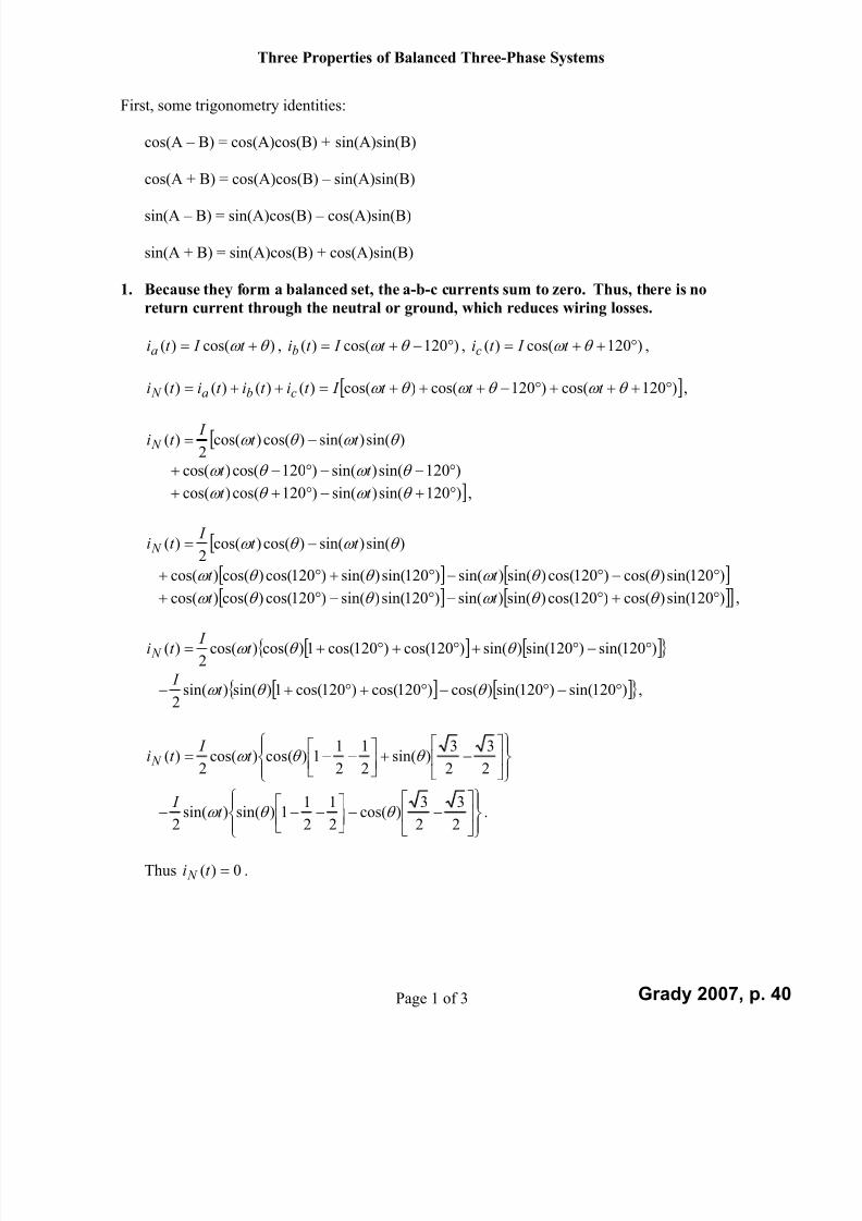
Three Properties of Balanced Three-Phase Systems
Page 1 of 3
First, some trigonometry identities:
cos(A – B) = cos(A)cos(B) + sin(A)sin(B)
cos(A + B) = cos(A)cos(B) – sin(A)sin(B)
sin(A – B) = sin(A)cos(B) – cos(A)sin(B)
sin(A + B) = sin(A)cos(B) + cos(A)sin(B)
1. Because they form a balanced set, the a-b-c currents sum to zero. Thus, there is no
return current through the neutral or ground, which reduces wiring losses.
)cos()( t I t ia , )120cos()( t I t ib , )120cos()( t I t ic ,
)120cos()120cos()cos()()()()( t t t I t it it it i cba N ,
)sin()sin()cos()cos(2
)( t t I
t i N
)120sin()sin()120cos()cos( t t
)120sin()sin()120cos()cos( t t ,
)sin()sin()cos()cos(2
)( t t I
t i N
)120sin()cos()120cos()sin()sin()120sin()sin()120cos()cos()cos( t t
)120sin()cos()120cos()sin()sin()120sin()sin()120cos()cos()cos( t t ,
)120sin()120sin()sin()120cos()120cos(1)cos()cos(2
)( t I
t i N
)120sin()120sin()cos()120cos()120cos(1)sin()sin(2
t I
,
2
3
2
3)sin(
2
1
2
11)cos()cos(
2)( t
I t i N
2
3
2
3)cos(2
1
2
11)sin()sin(2 t
I .
Thus 0)( t i N .
Grady 2007, p. 40

7/22/2019 Fundamentals Grady Notes June 2007 Print
http://slidepdf.com/reader/full/fundamentals-grady-notes-june-2007-print 41/388
Three Properties of Balanced Three-Phase Systems
Page 2 of 3
2. A N-wire system needs (N – 1) meters. A three-phase, four-wire system needs three
meters. A three-phase, three-wire system needs only two meters.
)()()()( t pt pt pt p cbatot ,
)()()()()()()()( ,,,, t it vt it vt it vt it v nref ncref cbref baref a ,
)()()()( t it it it icban
,
)()()()()()()( ,,, t it vt it vt it vt p cref cbref baref atot
)()()()(, t it it it v cbaref n ,
)()()()()()()()()()( ,,,,,, t it vt vt it vt vt it vt vt p cref nref cbref nref baref nref atot .
Thus, for three-phase, four-wire, three wattmeters are needed to compute
)()()()()()()( t it vt it vt it vt p ccnbbnaantot .
For three-phase, three-wire, the neutral wire is not present. Thus,
)()()( t it it i bac ,
and letting phase c become the reference, then
)()()()()()()()( t it it vt it vt it vt p bacnbbnaantot ,
)()()()()()()( t it vt vt it vt vt p bcnbnacnantot .
Thus, for three-phase, three-wire, two wattmeters are needed to compute
)()()()()( t it vt it vt p bbcaactot .
Three-phase,four wire system
a
bc
n
Reference
Grady 2007, p. 41
7/22/2019 Fundamentals Grady Notes June 2007 Print
http://slidepdf.com/reader/full/fundamentals-grady-notes-june-2007-print 42/388
Three Properties of Balanced Three-Phase Systems
Page 3 of 3
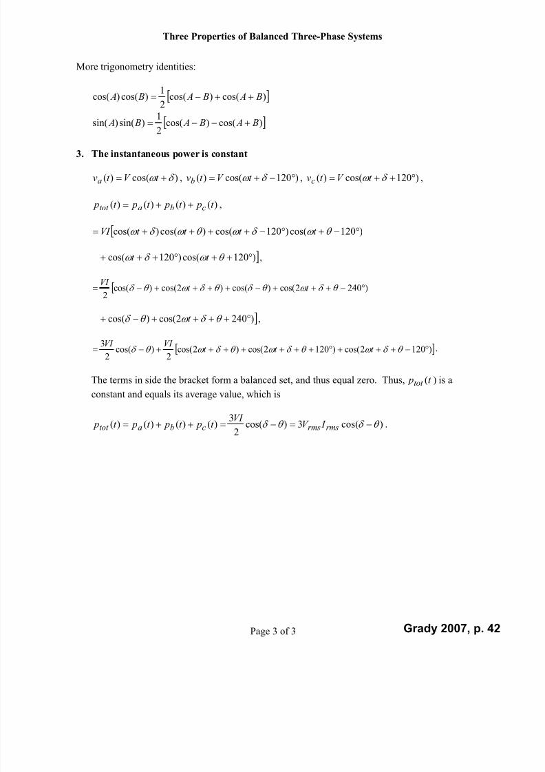
More trigonometry identities:
)cos()cos(2
1)cos()cos( B A B A B A
)cos()cos(
2
1)sin()sin( B A B A B A
3. The instantaneous power is constant
)cos()( t V t va , )120cos()( t V t vb , )120cos()( t V t vc ,
)()()()( t pt pt pt p cbatot ,
)120cos()120cos()cos()cos( t t t t VI
)120cos()120cos( t t ,
)2402cos()cos()2cos()cos(2
t t VI
)2402cos()cos( t ,
)1202cos()1202cos()2cos(2
)cos(2
3 t t t
VI VI .
The terms in side the bracket form a balanced set, and thus equal zero. Thus, )(t ptot
is a
constant and equals its average value, which is
)cos(3)cos(2
3)()()()( rmsrmscbatot I V
VI t pt pt pt p .
Grady 2007, p. 42

7/22/2019 Fundamentals Grady Notes June 2007 Print
http://slidepdf.com/reader/full/fundamentals-grady-notes-june-2007-print 43/388
2 b_
B a l a n c e d_ T h
r e e_ P h a s e_ P
h a s o r s . d o c
P a g e 1 o f 6
T h e p h a s o r s a r e r o t a t i n g c o u n t e r - c l o c k w i s e .
T h e m a g n i t u d e o f l i n e - t o - l i n e v o l t a g e p h a
s o r s i s
3 t i m e s t h e m a g n i t u d e
o f l i n e - t o - n e u t r a l v o l t a g e p h a s o
r s .
V b n
V a b
= V a n – V b n
V b c =
V b n – V c n
V a n
V c n
3
0 °
1 2 0 °
I m a g i n a r y
R e a l
V c a = V c n – V a n
Grady 2007, p. 43

7/22/2019 Fundamentals Grady Notes June 2007 Print
http://slidepdf.com/reader/full/fundamentals-grady-notes-june-2007-print 44/388
2 b_
B a l a n c e d_ T h
r e e_ P h a s e_ P
h a s o r s . d o c
P a g e 2 o f 6
C
o n s e r v a t i o n o f p o w e r r e q u i r e s t h a t t h e m a g n i t u d e s o f d e l t a c u r r e n t s I a b , I c a , a n d I b c a r e
3 1
t i m e s t h e
m a g n i t u d e o f l i n e c u r r e n t s I a , I b , I c .
V a
n
V b n
V c n
R e a l
I m a g i n a r y
V a b = V a n – V b n
V b c =
V b n – V c n
3 0 °
V c a = V c n – V a n
I a
I b
I c
I a b
I b c
I c a
I b I c
I a b
I c a
I b c
I a
a
c
b –
V a b
+
B a l a n c e d S e t s A d d
t o Z e r o i n B o t h
T i m e a n d P h a s o r D o m a i n s
I a + I b + I c = 0
V a n + V b n +
V c n = 0
V a b + V b c +
V c a = 0
L i n e c u r r e n t s I a , I b , a n d I c
D e l t a c u r r e n
t s I a b , I b c , a n d I c a
Grady 2007, p. 44

7/22/2019 Fundamentals Grady Notes June 2007 Print
http://slidepdf.com/reader/full/fundamentals-grady-notes-june-2007-print 45/388
2 b_
B a l a n c e d_ T h
r e e_ P h a s e_ P
h a s o r s . d o c
P a g e 3 o f 6
T h e T w o A b o v e L o a d s a r e E q u i v a l e n t i n B a l a n c e d S y s t e m s
( i . e . , s a m
e l i n e c u r r e n t s I a , I b , I c a n d p h a s e - t o - p h a s e v o l t a g e s V
a b , V b c , V c a i n b o t h c a s e s )
3 Z
3 Z
3 Z
a
c
b
–
V a b
+
I a I b I c
Z
Z
Z
a
c
b
–
V a b
+
I a I b I c
n
Grady 2007, p. 45

7/22/2019 Fundamentals Grady Notes June 2007 Print
http://slidepdf.com/reader/full/fundamentals-grady-notes-june-2007-print 46/388
2 b_
B a l a n c e d_ T h
r e e_ P h a s e_ P
h a s o r s . d o c
P a g e 4 o f 6
T h e T w o A b o v e S o
u r c e s a r e E q u i v a l e n t i n B a l a n c e d S y s t e m s
( i . e . , s a m e l i n e c u r r e n t s I a , I b , I c a
n d p h a s e - t o - p h a s e v o l t a g e s
V a b , V b c , V c a i n b o t h c a s e s )
a
c
b
–
V a b
+
I a I b I c
V a n
a
c
b
–
V a b
+
I a I b I c
n
+
–
Grady 2007, p. 46
7/22/2019 Fundamentals Grady Notes June 2007 Print
http://slidepdf.com/reader/full/fundamentals-grady-notes-june-2007-print 47/388
2 b_
B a l a n c e d_ T h
r e e_ P h a s e_ P
h a s o r s . d o c
P a g e 5 o f 6
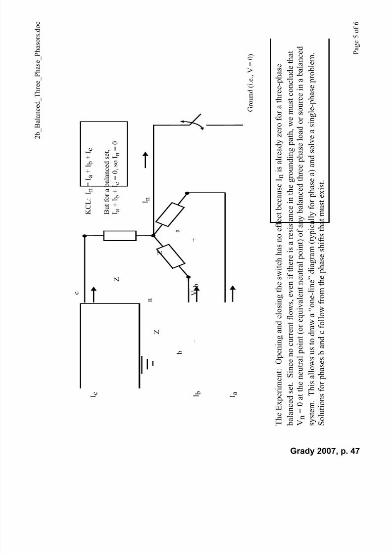
Z
Z
Z
a
b
–
V a b
+
I a I b I c
c n
I n
K C L : I n =
I a + I b + I c
B u t f o r a b a l a n c e d s e t ,
I a + I b + I c
= 0 , s o I n = 0
G r o u n d
( i . e . , V = 0 )
T h e E x p e r i m e n t :
O p e n i n g a n d c l o s i n g t h e s w
i t c h h a s n o e f f e c t b e c a u s e
I n i s a l r e a d y z e r o f o r a t h r e e - p h a s e
b a l a n c e d s e t . S i n
c e n o c u r r e n t f l o w s , e v e n i f
t h e r e i s a r e s i s t a n c e i n t h e g r o u n d i n g p a t h , w e m u s t c o
n c l u d e t h a t
V n = 0 a t t h e n e u t r a l p o i n t ( o r e q u i v a l e n t n e u
t r a l p o i n t ) o f a n y b a l a n c e d
t h r e e p h a s e l o a d o r s o u r c e i n a b a l a n c e d
s y s t e m . T h i s a l l o
w s u s t o d r a w a “ o n e - l i n e ”
d i a g r a m ( t y p i c a l l y f o r p h a s e a ) a n d s o l v e a s i n g l e - p h a s
e p r o b l e m .
S o l u t i o n s f o r p h a s e s b a n d c f o l l o w f r o m t h e
p h a s e s h i f t s t h a t m u s t e x i s t .
Grady 2007, p. 47

7/22/2019 Fundamentals Grady Notes June 2007 Print
http://slidepdf.com/reader/full/fundamentals-grady-notes-june-2007-print 48/388
2 b_
B a l a n c e d_ T h
r e e_ P h a s e_ P
h a s o r s . d o c
P a g e 6 o f 6
B a l a n c e d t h r e e - p h a s e s y s t e m s , n o m a t t e r i f t h e y a r e d e l t a
c o n n e c t e d , w y
e c o n n e c t e d , o r a m i x , a r e e a s y t o s o l v e i f y o u
f o l l o w t h e s e s t e p s :
1 . C o n v e r t t h
e e n t i r e c i r c u i t t o a n e q u i v a l e n t w y e w i t h a
g r o u n d e d n e u t r a l .
2 . D r a w t h e o
n e - l i n e d i a g r a m f o r p h a s e a , r e c
o g n i z i n g t h a t
p h a s e a h a s o n e t h i r d o f t h e P a n d Q .
3 . S o l v e t h e o n e - l i n e d i a g r a m f o r l i n e - t o - n e u t r a l v o l t a g e s a n d
l i n e c u r r e n
t s .
4 . I f n e e d e d ,
c o m p u t e l i n e - t o - n e u t r a l v o l t a g e s a n d l i n e c u r r e n t s
f o r p h a s e s
b a n d c u s i n g t h e ± 1 2 0 ° r e l a t i o n
s h i p s .
5 . I f n e e d e d ,
c o m p u t e l i n e - t o - l i n e v o l t a g e s a n
d d e l t a c u r r e n t s
u s i n g t h e
3 a n d ± 3 0 ° r e l a t i o n s h i p s .
a n
a n
Z l o a d
+ V a n –
Z l i n e
I a a
c
b
–
V a b
+
3 Z l o a d
a
c
b
I b I a I c
Z l i n e
Z l i n e
Z l i n e
3 Z l o a d
3 Z l o a d
T
h e “ O n e - L i n e ”
D i a g r a m
Grady 2007, p. 48

7/22/2019 Fundamentals Grady Notes June 2007 Print
http://slidepdf.com/reader/full/fundamentals-grady-notes-june-2007-print 49/388
Grady 2007, p. 49
7/22/2019 Fundamentals Grady Notes June 2007 Print
http://slidepdf.com/reader/full/fundamentals-grady-notes-june-2007-print 50/388
Grady 2007, p. 50

7/22/2019 Fundamentals Grady Notes June 2007 Print
http://slidepdf.com/reader/full/fundamentals-grady-notes-june-2007-print 51/388
Grady 2007, p. 51

7/22/2019 Fundamentals Grady Notes June 2007 Print
http://slidepdf.com/reader/full/fundamentals-grady-notes-june-2007-print 52/388
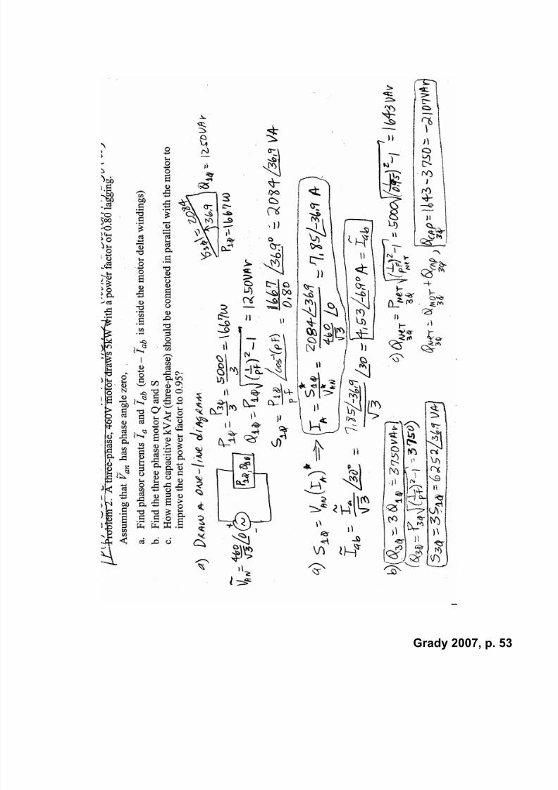
A three-phase, 460V motor draws 5kW with a power factor of 0.80 lagging. Assuming that anV ~
has phase angle zero,
a. Find phasor currents a I ~
and ab I ~
(note – ab I ~
is inside the motor delta windings)
b. Find the three phase motor Q and S
c. How much capacitive kVAr (three-phase) should be connected in parallel with the motor toimprove the net power factor to 0.95?
d. Assuming no change in supply voltage, what will be the new a I ~
after the kVArs are added?
Grady 2007, p. 52
7/22/2019 Fundamentals Grady Notes June 2007 Print
http://slidepdf.com/reader/full/fundamentals-grady-notes-june-2007-print 53/388
Grady 2007, p. 53
7/22/2019 Fundamentals Grady Notes June 2007 Print
http://slidepdf.com/reader/full/fundamentals-grady-notes-june-2007-print 54/388
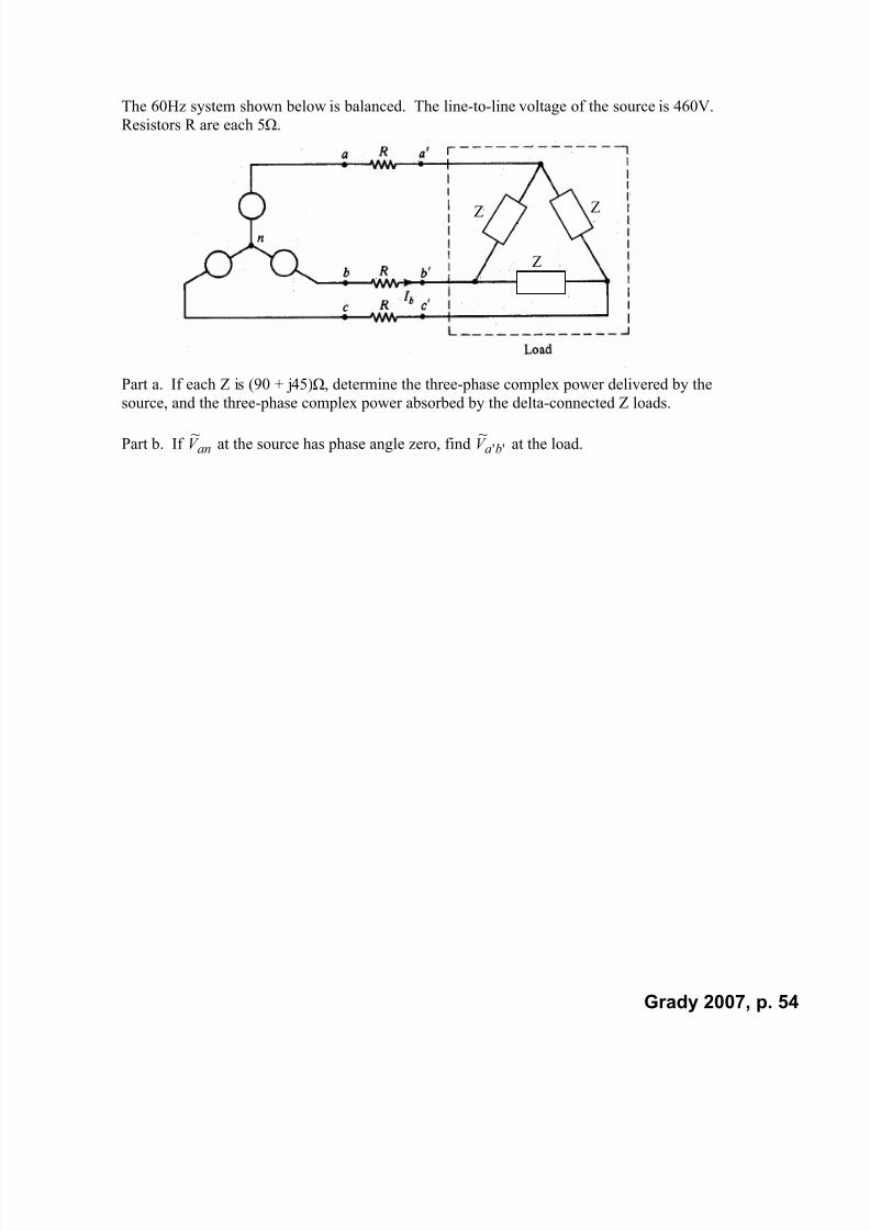
The 60Hz system shown below is balanced. The line-to-line voltage of the source is 460V.
Resistors R are each 5.
Part a. If each Z is (90 + j45), determine the three-phase complex power delivered by the
source, and the three-phase complex power absorbed by the delta-connected Z loads.
Part b. If anV ~
at the source has phase angle zero, find ''~
baV at the load.
Z
ZZ
Grady 2007, p. 54

7/22/2019 Fundamentals Grady Notes June 2007 Print
http://slidepdf.com/reader/full/fundamentals-grady-notes-june-2007-print 55/388
Grady 2007, p. 55

7/22/2019 Fundamentals Grady Notes June 2007 Print
http://slidepdf.com/reader/full/fundamentals-grady-notes-june-2007-print 56/388
Grady 2007, p. 56
7/22/2019 Fundamentals Grady Notes June 2007 Print
http://slidepdf.com/reader/full/fundamentals-grady-notes-june-2007-print 57/388
Grady 2007, p. 57
7/22/2019 Fundamentals Grady Notes June 2007 Print
http://slidepdf.com/reader/full/fundamentals-grady-notes-june-2007-print 58/388
Grady 2007, p. 58
7/22/2019 Fundamentals Grady Notes June 2007 Print
http://slidepdf.com/reader/full/fundamentals-grady-notes-june-2007-print 59/388
Grady 2007, p. 59
7/22/2019 Fundamentals Grady Notes June 2007 Print
http://slidepdf.com/reader/full/fundamentals-grady-notes-june-2007-print 60/388
Grady 2007, p. 60

7/22/2019 Fundamentals Grady Notes June 2007 Print
http://slidepdf.com/reader/full/fundamentals-grady-notes-june-2007-print 61/388
Grady 2007, p. 61

7/22/2019 Fundamentals Grady Notes June 2007 Print
http://slidepdf.com/reader/full/fundamentals-grady-notes-june-2007-print 62/388
Grady 2007, p. 62

7/22/2019 Fundamentals Grady Notes June 2007 Print
http://slidepdf.com/reader/full/fundamentals-grady-notes-june-2007-print 63/388
Grady 2007, p. 63

7/22/2019 Fundamentals Grady Notes June 2007 Print
http://slidepdf.com/reader/full/fundamentals-grady-notes-june-2007-print 64/388
Grady 2007, p. 64
7/22/2019 Fundamentals Grady Notes June 2007 Print
http://slidepdf.com/reader/full/fundamentals-grady-notes-june-2007-print 65/388
Grady 2007, p. 65
7/22/2019 Fundamentals Grady Notes June 2007 Print
http://slidepdf.com/reader/full/fundamentals-grady-notes-june-2007-print 66/388
Grady 2007, p. 66
7/22/2019 Fundamentals Grady Notes June 2007 Print
http://slidepdf.com/reader/full/fundamentals-grady-notes-june-2007-print 67/388
Grady 2007, p. 67
7/22/2019 Fundamentals Grady Notes June 2007 Print
http://slidepdf.com/reader/full/fundamentals-grady-notes-june-2007-print 68/388
Grady 2007, p. 68
7/22/2019 Fundamentals Grady Notes June 2007 Print
http://slidepdf.com/reader/full/fundamentals-grady-notes-june-2007-print 69/388
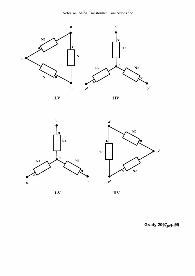
Notes_on_ANSI_Transformer_Connections.doc
Page 1 of 1
N1
N1
N1
a
b
c
N2
N2 N2n
a’
b’c'
LV HV
N1
N1 N1n
N2
N2
N2
a
bc
b’
a’
c’
LV HV
Grady 2007, p. 69
7/22/2019 Fundamentals Grady Notes June 2007 Print
http://slidepdf.com/reader/full/fundamentals-grady-notes-june-2007-print 70/388
Grady 2007, p. 70

7/22/2019 Fundamentals Grady Notes June 2007 Print
http://slidepdf.com/reader/full/fundamentals-grady-notes-june-2007-print 71/388
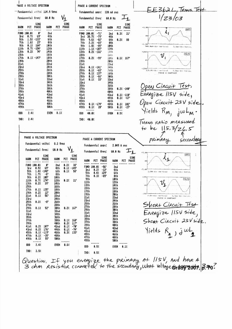
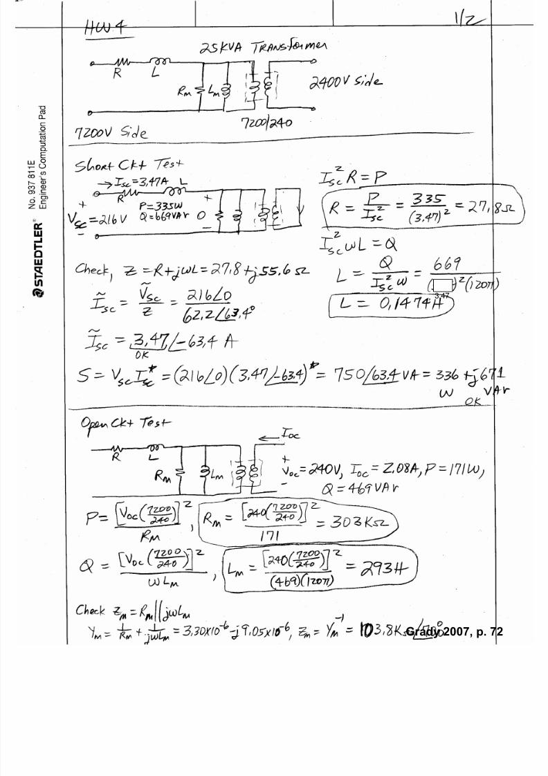
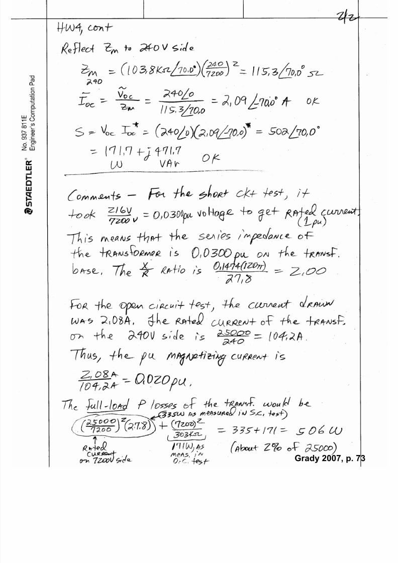
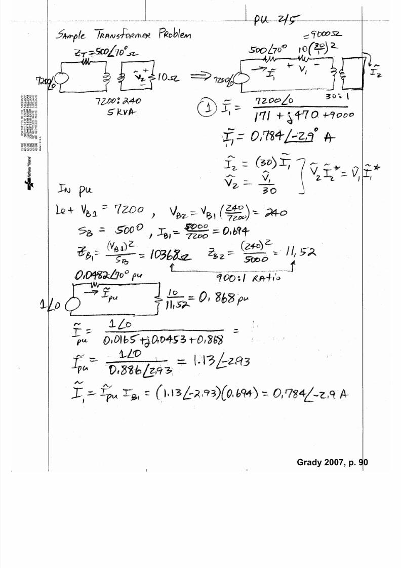
The following data were taken for a 25kVA, 7200/240V transformer:
Short Circuit Test: 240V side short-circuited, 7200V side energized at reduced voltage.The measurements (on the 7200V side) are Irms = 3.47A (i.e., rated current), Vrms =
216V, P = 335W, Q = 669VAr.
Open Circuit Test: 7200V side open-circuited, 240V side energized. The measurements
(on the 240V side) are Vrms = 240V (i.e., rated voltage), Irms = 2.08A, P = 171W, Q =469VAr.
Draw the transformer equivalent circuit with all four circuit parameters (i.e., R, Ll, Lm, R m)
shown on the 7200V side.
Grady 2007, p. 71
7/22/2019 Fundamentals Grady Notes June 2007 Print
http://slidepdf.com/reader/full/fundamentals-grady-notes-june-2007-print 72/388
Grady 2007, p. 72
3.47
7/22/2019 Fundamentals Grady Notes June 2007 Print
http://slidepdf.com/reader/full/fundamentals-grady-notes-june-2007-print 73/388
Grady 2007, p. 73

7/22/2019 Fundamentals Grady Notes June 2007 Print
http://slidepdf.com/reader/full/fundamentals-grady-notes-june-2007-print 74/388
EE369/394J, Test #4, Sept. 24, 2004. Name _______________________________________One sheet of notes permitted. Show all steps.
The following data were taken for a 75kVA, 7200/480V transformer:
Short Circuit Test: 480V side short-circuited, 7200V side energized at reduced voltage. The
measurements (on the 7200V side) are Irms = 10.0A, Vrms = 144V, P = 750W.
Open Circuit Test: 7200V side open-circuited, 480V side energized. The measurements (on the
480V side) are Vrms = 480V, Irms = 1.50A, P = 500W.
Draw the transformer equivalent circuit with all four circuit parameters (i.e., R, Ll, Lm, R m) shown on
the 7200V side. Hint – remember that rmsrms I V S ,222 Q P S .
Grady 2007, p. 74

7/22/2019 Fundamentals Grady Notes June 2007 Print
http://slidepdf.com/reader/full/fundamentals-grady-notes-june-2007-print 75/388
Grady 2007, p. 75

7/22/2019 Fundamentals Grady Notes June 2007 Print
http://slidepdf.com/reader/full/fundamentals-grady-notes-june-2007-print 76/388
Open circuit and short circuit tests are performed on a single-phase, 7200/240V, 25kVA, 60Hz
distribution transformer. The results are:
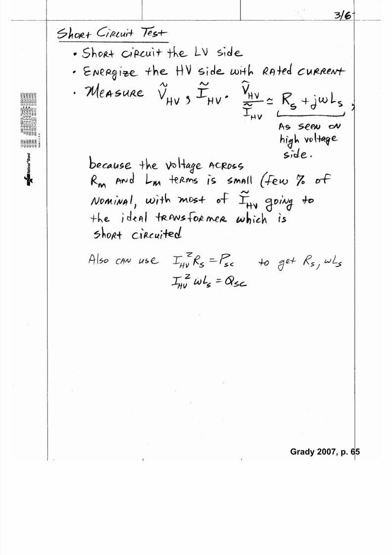
Short circuit test (short circuit the low-voltage side, energize the high-voltage side so thatrated current flows, and measure Psc and Qsc). Measured Psc = 400W, Qsc = 200VAr.
Open circuit test (open circuit the high-voltage side, apply rated voltage to the low-voltage
side, and measure Poc and Qoc). Measured Poc = 100W, Qoc = 250VAr.
Determine the four impedance values (in ohms) for the transformer model shown.
Rs jXs
IdealTransformer
7200/240VRm jXm
7200V 240V
Grady 2007, p. 76

7/22/2019 Fundamentals Grady Notes June 2007 Print
http://slidepdf.com/reader/full/fundamentals-grady-notes-june-2007-print 77/388
Grady 2007, p. 77

7/22/2019 Fundamentals Grady Notes June 2007 Print
http://slidepdf.com/reader/full/fundamentals-grady-notes-june-2007-print 78/388
Grady, Transformers, June 2007, Page 1
Transformers
Transformers. Transformer phase shift. Wye-delta connections and impact on zero sequence.
Inductance and capacitance calculations for transmission lines. GMR, GMD, L, and C matrices,
effect of ground conductivity. Underground cables.
Equivalent Circuits
The standard transformer equivalent circuit used in power system simulation is shown below,
where the R and X terms represent the series resistance and leakage reactance, and N1 and N2
represent the transformer turns. Note that the shunt terms are usually ignored in the model..
R jX
N1 N2
Figure 1. Power System Model for Transformer
Three-phase transformers can consist of either three separate single-phase transformers, or three
windings on a three-legged, four-legged, or five-legged core. The high-voltage and low-voltage
sides can be connected independently in either wye or delta.
A B C
High-Voltage Side
Low-Voltage Side
Figure 2. A Three-Phase Ground-Wye Grounded-Wye Transformer
Grady 2007, p. 78
7/22/2019 Fundamentals Grady Notes June 2007 Print
http://slidepdf.com/reader/full/fundamentals-grady-notes-june-2007-print 79/388
Grady, Transformers, June 2007, Page 2
A B C
High-Voltage Side
Low-Voltage Side
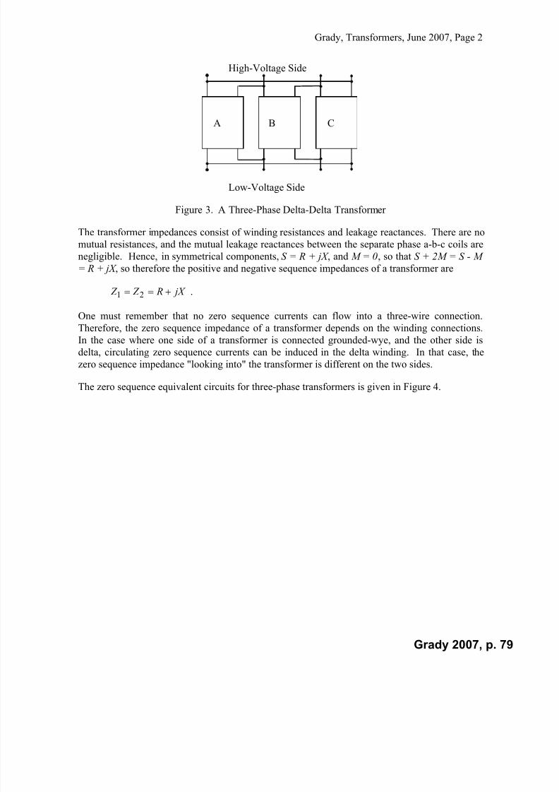
Figure 3. A Three-Phase Delta-Delta Transformer
The transformer impedances consist of winding resistances and leakage reactances. There are no
mutual resistances, and the mutual leakage reactances between the separate phase a-b-c coils are
negligible. Hence, in symmetrical components, S = R + jX , and M = 0, so that S + 2M = S - M
= R + jX , so therefore the positive and negative sequence impedances of a transformer are
jX R Z Z 21 .
One must remember that no zero sequence currents can flow into a three-wire connection.
Therefore, the zero sequence impedance of a transformer depends on the winding connections.
In the case where one side of a transformer is connected grounded-wye, and the other side is
delta, circulating zero sequence currents can be induced in the delta winding. In that case, the
zero sequence impedance "looking into" the transformer is different on the two sides.
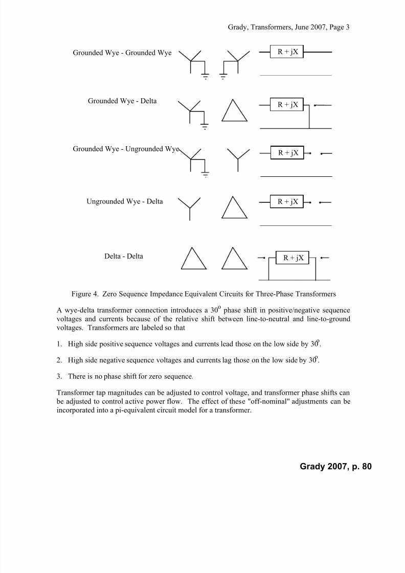
The zero sequence equivalent circuits for three-phase transformers is given in Figure 4.
Grady 2007, p. 79
7/22/2019 Fundamentals Grady Notes June 2007 Print
http://slidepdf.com/reader/full/fundamentals-grady-notes-june-2007-print 80/388
Grady, Transformers, June 2007, Page 3
Grounded Wye - Grounded Wye
Grounded Wye - DeltaR + jX
Grounded Wye - Ungrounded WyeR + jX
R + jXUngrounded Wye - Delta
R + jXDelta - Delta
R + jX
Figure 4. Zero Sequence Impedance Equivalent Circuits for Three-Phase Transformers
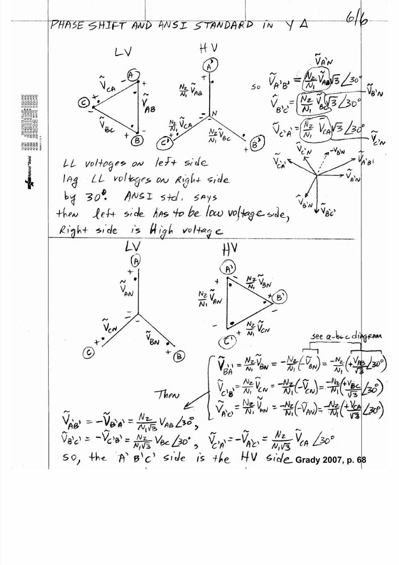
A wye-delta transformer connection introduces a 30o phase shift in positive/negative sequence
voltages and currents because of the relative shift between line-to-neutral and line-to-ground
voltages. Transformers are labeled so that
1. High side positive sequence voltages and currents lead those on the low side by 30o.
2. High side negative sequence voltages and currents lag those on the low side by 30o.
3. There is no phase shift for zero sequence.
Transformer tap magnitudes can be adjusted to control voltage, and transformer phase shifts can
be adjusted to control active power flow. The effect of these "off-nominal" adjustments can be
incorporated into a pi-equivalent circuit model for a transformer.
Grady 2007, p. 80

7/22/2019 Fundamentals Grady Notes June 2007 Print
http://slidepdf.com/reader/full/fundamentals-grady-notes-june-2007-print 81/388
Grady, Transformers, June 2007, Page 4
y
Ii ---> Ik --->Bus i
Bus k t / :1
Bus k'
Figure 5. Off-Nominal Transformer Circuit Model
Assume that the transformer in Figure 5 has complex "off-nominal" tap t t and series
admittance y. The relationship between the voltage on opposite sides of the transformer tap is
t
ik
t
V V
~~
' , and since the power on both sides of the ideal transformer must be the same, then
*''
* ~~~~k k ii I V I V , implying that t ik t I I
~~' . Now, suppose that the transformer can be
modeled by the following pi-equivalent circuit of Figure 6:
yik
Ii --->
Bus i
yii
Bus k
<--- -Ik
ykk
Figure 6. Pi-Equivalent Model of Transformer
Admittances yii, yik , and ykk can be found so that the above circuit is equivalent to Figure 5. This
can be accomplished by forcing the terminal behavior to be the same. For the above circuit, the
appropriate equations are
iiiik k ii yV yV V I ~~~~
, and kk k ik ik k yV yV V I ~~~~
,
or in matrix form
k
i
ik kk ik
ik ik ii
k
i
V
V
y y y
y y y
I
I ~
~
~
~
.
For Figure 5, the terminal equations are
yV t
V yV V I k
t
ik k k
~~
~~~'
,
and since
Grady 2007, p. 81

7/22/2019 Fundamentals Grady Notes June 2007 Print
http://slidepdf.com/reader/full/fundamentals-grady-notes-june-2007-print 82/388
Grady, Transformers, June 2007, Page 5
t
k i
t
I I
~~
,
then
yt
V
t t
V I
t
k
t t
ii
~~~ .
In matrix form,
k
i
t
t t t
k
i
V
V
yt
y
t
y
t t
y
I
I ~
~
~
~
.
Comparing the two sets of terminal equations shows that equality can be reached if the shunt
branch in the equivalent circuit, yik , can have two values:
t ik
t
y y
from the perspective of Kirchhoff's current law at bus i,
t ik
t
y y
from the perspective of Kirchhoff's current law at bus k.
Note that if the tap does not include an off-nominal phase shift, thent
y yik from either
direction.
Next, solving for yii and ykk yields
1
1
t t t t t ii
t t
y
t
y
t t
y y
,
t t kk
t y
t
y y y
11 .
Neutral Grounding Impedance
If the wye-side of a transformer or wye-connected load is grounded through a grounding
impedance Z g , the grounding impedance is "invisible" to the positive and negative sequence
currents since their corresponding voltages at the wye-point is always zero due to symmetry.
However, since the neutral current is three-times the zero sequence current, the voltage drop on
the grounding impedance is 3 I ao. For that reason, the zero sequence equivalent circuit for a
grounding impedance must contain 3 Z g .
Grady 2007, p. 82

7/22/2019 Fundamentals Grady Notes June 2007 Print
http://slidepdf.com/reader/full/fundamentals-grady-notes-june-2007-print 83/388
Grady, Transformers, June 2007, Page 6
Z Z Z
Zg
Zao = Z + 3Zg+
-
Vao = 3 Iao Zg
Iao Iao Iao
Za1 = Za2 = Z
Figure 7. Effect of Grounding Impedance on Sequence Impedances
Grady 2007, p. 83

7/22/2019 Fundamentals Grady Notes June 2007 Print
http://slidepdf.com/reader/full/fundamentals-grady-notes-june-2007-print 84/388
3l_ANSI_Transformer_Wye_Delta_Labeling.doc
Page 1 of 1
N1
N1
N1
a
b
c
N2
N2 N2n
a’
b’c'
LV HV
N1
N1 N1n
N2
N2
N2
a
bc
b’
a’
c’
LV HV
Grady 2007, p. 84

7/22/2019 Fundamentals Grady Notes June 2007 Print
http://slidepdf.com/reader/full/fundamentals-grady-notes-june-2007-print 85/388
Grady 2007, p. 85
7/22/2019 Fundamentals Grady Notes June 2007 Print
http://slidepdf.com/reader/full/fundamentals-grady-notes-june-2007-print 86/388
Grady, Per Unit, June 2007, Page 1
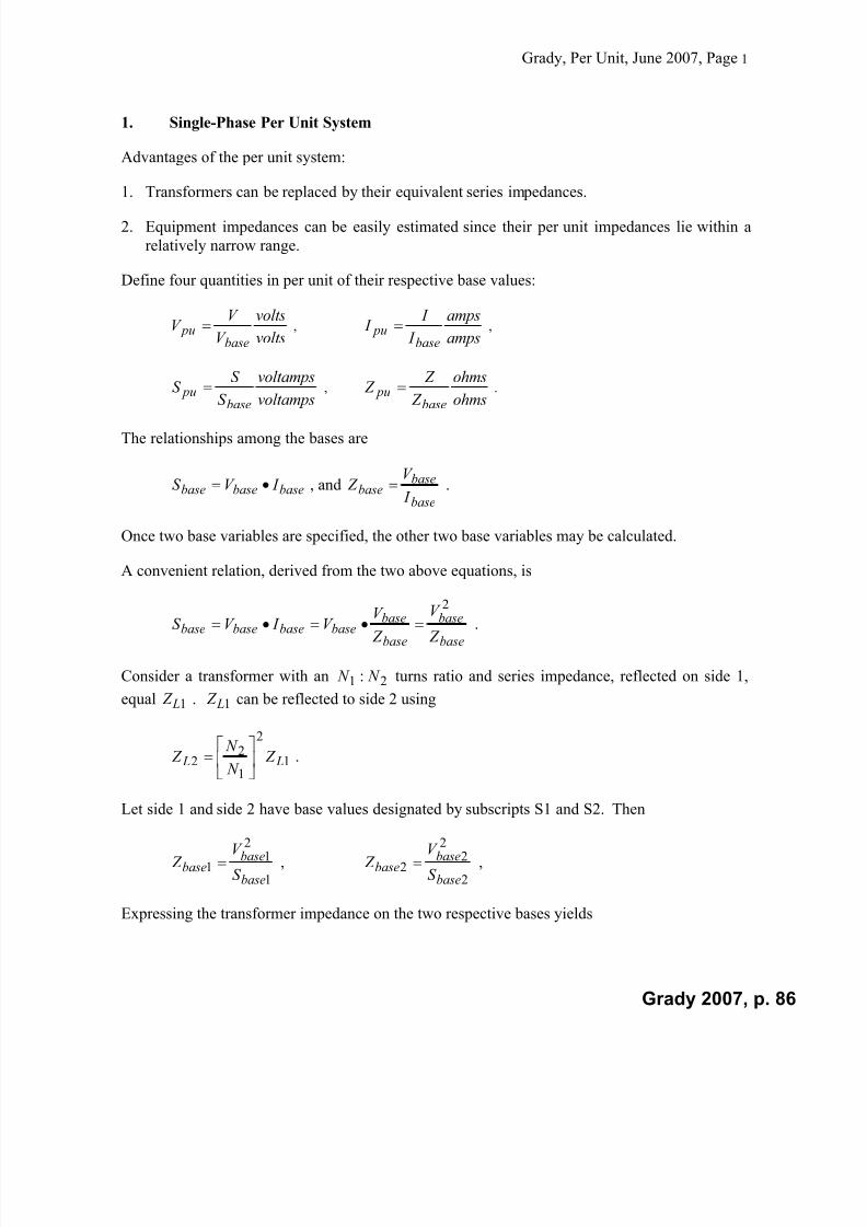
1. Single-Phase Per Unit System
Advantages of the per unit system:
1. Transformers can be replaced by their equivalent series impedances.
2. Equipment impedances can be easily estimated since their per unit impedances lie within a
relatively narrow range.
Define four quantities in per unit of their respective base values:
volts
volts
V
V V
base pu ,
amps
amps
I
I I
base pu ,
voltamps
voltamps
S
S S
base
pu ,ohms
ohms
Z
Z Z
base
pu .
The relationships among the bases are
basebasebase I V S , andbase
basebase
I
V Z .
Once two base variables are specified, the other two base variables may be calculated.
A convenient relation, derived from the two above equations, is
base
base
base
basebasebasebasebase
Z V
Z V V I V S
2
.
Consider a transformer with an 21 : N N turns ratio and series impedance, reflected on side 1,
equal 1 L Z . 1 L Z can be reflected to side 2 using
1
2
1
22 L L Z
N
N Z
.
Let side 1 and side 2 have base values designated by subscripts S1 and S2. Then
1
21
1base
basebase
S
V Z ,
2
22
2base
basebase
S
V Z ,
Expressing the transformer impedance on the two respective bases yields
Grady 2007, p. 86

7/22/2019 Fundamentals Grady Notes June 2007 Print
http://slidepdf.com/reader/full/fundamentals-grady-notes-june-2007-print 87/388
Grady, Per Unit, June 2007, Page 2
21
111
base
base L PU L
V
S Z Z ,
22
222
base
base L PU L
V
S Z Z .
If 21 B B S S , the two above equations may be combined so that
PU Lbase
base PU L Z
V
V
N
N Z 1
2
2
12
1
22
.
Substituting the relation between 1 L Z and 2 L Z yields
PU Lbase
base PU L Z
V
V
N
N Z 1
2
2
12
1
22
.
Therefore, if12
12
N
N
V
V
basebase , then PU L PU L Z Z 12 .
Hence, if a common voltampere base is chosen on both sides of the transformer, and if the
voltage bases are chosen so that they vary according to the transformer turns ratio, then the per
unit series impedance of the transformer is the same value on both sides.
When analyzing a circuit with many transformers, a common voltampere base should be chosen
throughout the circuit, and a voltage base should be chosen at one location. The voltage base
must vary across the circuit according to the transformer turns ratios.
When analyzing a circuit in per unit, if the bases are chosen according to the above rules,
transformers can be replaced by their equivalent per unit series impedances, and their turns can
be ignored.
A manufacturer usually provides the impedance of a transformer on the transformer's rated
voltage and power bases. However, when solving a power network circuit, the power and
voltage bases must vary according to the above rules, and they may not equal the manufacturer-
specified bases. Per unit impedances, specified on one base, may be converted to a new base as
follows:
Given
old base
old PU Z
Z Z
,
, , on bases old baseV , and old baseS , , new PU Z , on new bases
newbaseV , and newbaseS , is
2,
,
,
2,
,,
,,
,,
newbase
newbase
old base
old baseold PU
newbase
old baseold PU
newbase
ohmsnew PU
V
S
S
V Z
Z
Z Z
Z
Z Z .
Grady 2007, p. 87

7/22/2019 Fundamentals Grady Notes June 2007 Print
http://slidepdf.com/reader/full/fundamentals-grady-notes-june-2007-print 88/388
Grady, Per Unit, June 2007, Page 3
2. Three-Phase Per Unit System
The same advantages apply to a three-phase system if the following rules are obeyed:
1. A common three-phase voltampere base is used throughout the system, where
1,3, 3 basebase S S .
2. Once selected at a point in the network, the three-phase voltage base must vary according to
the line-to-line transformer turns ratios.
Convenient formulas relating single-phase to three-phase bases are given below.
baseneutral linebasebase I V S ,1, ,
1,3, 3 basebase S S ,
3,
2,
3,
,
2
1,
2,
3/
3/
base
linelinebase
base
linelinebase
base
neutral linebasebase
S
V
S
V
S
V Z
.
Grady 2007, p. 88

7/22/2019 Fundamentals Grady Notes June 2007 Print
http://slidepdf.com/reader/full/fundamentals-grady-notes-june-2007-print 89/388
Grady 2007, p. 89
7/22/2019 Fundamentals Grady Notes June 2007 Print
http://slidepdf.com/reader/full/fundamentals-grady-notes-june-2007-print 90/388
Grady 2007, p. 90

7/22/2019 Fundamentals Grady Notes June 2007 Print
http://slidepdf.com/reader/full/fundamentals-grady-notes-june-2007-print 91/388
Grady 2007, p. 91

7/22/2019 Fundamentals Grady Notes June 2007 Print
http://slidepdf.com/reader/full/fundamentals-grady-notes-june-2007-print 92/388
Grady 2007, p. 92
4 of 5
7/22/2019 Fundamentals Grady Notes June 2007 Print
http://slidepdf.com/reader/full/fundamentals-grady-notes-june-2007-print 93/388
Grady 2007, p. 93
5 of 5

7/22/2019 Fundamentals Grady Notes June 2007 Print
http://slidepdf.com/reader/full/fundamentals-grady-notes-june-2007-print 94/388
Find the magnitude of the line-to-line voltages on the 12.47kV side of the transformer.
Z = 0.05pu
15kVA
12.47kV/480V,
X/R = 1
Transformer
(GY-GY)
V(line-to-line) = 460V,
three-phase P = 10kW,
pf = 0.90 lagging
Supply network
Grady 2007, p. 94

7/22/2019 Fundamentals Grady Notes June 2007 Print
http://slidepdf.com/reader/full/fundamentals-grady-notes-june-2007-print 95/388
Grady 2007, p. 95

7/22/2019 Fundamentals Grady Notes June 2007 Print
http://slidepdf.com/reader/full/fundamentals-grady-notes-june-2007-print 96/388
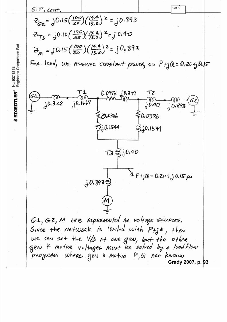
Information for a small power system is shown below. Per unit values are given on the equipment bases.
Using a 138kV, 100MVA base in the transmission lines, draw the per unit diagram. Assume that no
current is flowing in the network, so that all generator and motor voltages are 1.0pu in your final diagram.
Trans1
Gen1
X” = 0.15
40MVA
20kV
Trans1
X = 0.16
60MVA
18kV/138kV
TLine1
Line1
R = 10
X = 60
Trans2Trans2
X=0.14
50MVA
20kV/138kV
TLine2
Line2
R = 10
X = 60
Trans3
Trans3X = 0.10
40MVA
13.8kV/138kV
Motor
X” = 0.10
25MVA
13.2kV
Gen2
X” = 0.15
35MVA
22kV
Grady 2007, p. 96

7/22/2019 Fundamentals Grady Notes June 2007 Print
http://slidepdf.com/reader/full/fundamentals-grady-notes-june-2007-print 97/388
Grady 2007, p. 97

7/22/2019 Fundamentals Grady Notes June 2007 Print
http://slidepdf.com/reader/full/fundamentals-grady-notes-june-2007-print 98/388
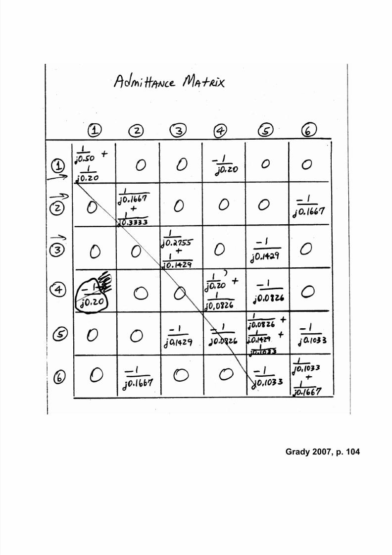
4g_Grainger_Stevenson_Problems.doc
Should be 50 MVA
Bus1 Bus2
Bus3
Bus5Bus6Bus4
Grady 2007, p. 98
7/22/2019 Fundamentals Grady Notes June 2007 Print
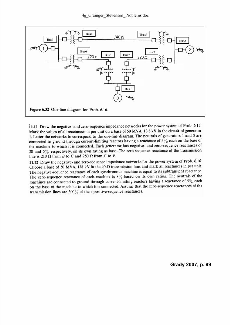
http://slidepdf.com/reader/full/fundamentals-grady-notes-june-2007-print 99/388
4g_Grainger_Stevenson_Problems.doc
Bus1 Bus2
Bus3
Bus4 Bus5
Bus6 Bus7Bus8 Bus9
Grady 2007, p. 99

7/22/2019 Fundamentals Grady Notes June 2007 Print
http://slidepdf.com/reader/full/fundamentals-grady-notes-june-2007-print 100/388
4g_Grainger_Stevenson_Problems.doc
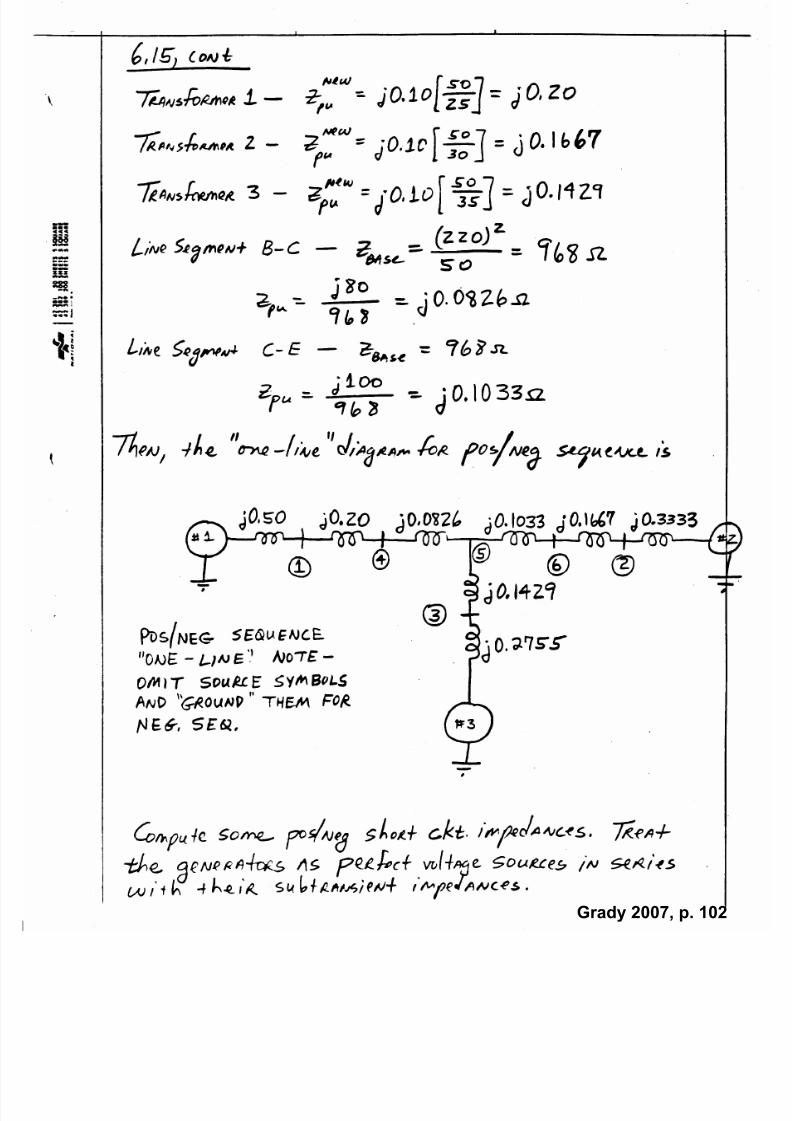
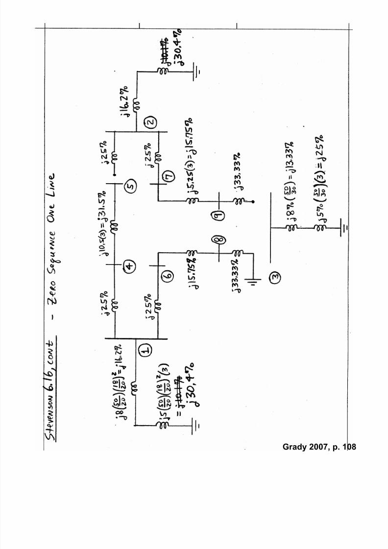
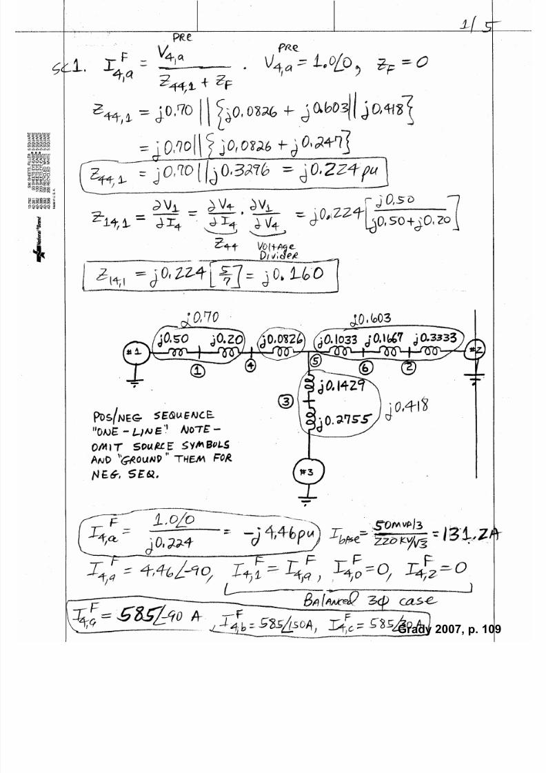
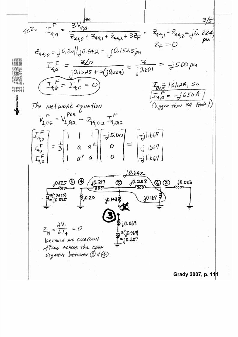
Short Circuit Calculation
(Based upon Grainger/Stevenson Problem 6.15/11.11)
SC Problem 1. A three-phase balanced fault, with ZF = 0, occurs at Bus 4. Determine
a. F a I 4 (in per unit and in amps)
b. Phasor abc line-to-neutral voltages at the terminals of Gen 1
c. Phasor abc currents flowing out of Gen 1 (in per unit and in amps)
SC Problem 2. Repeat Problem 1, again with ZF = 0, but with a single-phase-to-ground
fault at Bus 4, phase a.
In both Problems 1 and 2, make sure that you add in the transformer phase shifts,
assuming that pre-fault Van in the transmission line has reference phase angle 0.
Grady 2007, p. 100

7/22/2019 Fundamentals Grady Notes June 2007 Print
http://slidepdf.com/reader/full/fundamentals-grady-notes-june-2007-print 101/388
Grady 2007, p. 101
7/22/2019 Fundamentals Grady Notes June 2007 Print
http://slidepdf.com/reader/full/fundamentals-grady-notes-june-2007-print 102/388
Grady 2007, p. 102

7/22/2019 Fundamentals Grady Notes June 2007 Print
http://slidepdf.com/reader/full/fundamentals-grady-notes-june-2007-print 103/388
Grady 2007, p. 103
7/22/2019 Fundamentals Grady Notes June 2007 Print
http://slidepdf.com/reader/full/fundamentals-grady-notes-june-2007-print 104/388
Grady 2007, p. 104

7/22/2019 Fundamentals Grady Notes June 2007 Print
http://slidepdf.com/reader/full/fundamentals-grady-notes-june-2007-print 105/388
Grady 2007, p. 105

7/22/2019 Fundamentals Grady Notes June 2007 Print
http://slidepdf.com/reader/full/fundamentals-grady-notes-june-2007-print 106/388
Grady 2007, p. 106

7/22/2019 Fundamentals Grady Notes June 2007 Print
http://slidepdf.com/reader/full/fundamentals-grady-notes-june-2007-print 107/388
Grady 2007, p. 107
7/22/2019 Fundamentals Grady Notes June 2007 Print
http://slidepdf.com/reader/full/fundamentals-grady-notes-june-2007-print 108/388
Grady 2007, p. 108
7/22/2019 Fundamentals Grady Notes June 2007 Print
http://slidepdf.com/reader/full/fundamentals-grady-notes-june-2007-print 109/388
Grady 2007, p. 109

7/22/2019 Fundamentals Grady Notes June 2007 Print
http://slidepdf.com/reader/full/fundamentals-grady-notes-june-2007-print 110/388
Grady 2007, p. 110
7/22/2019 Fundamentals Grady Notes June 2007 Print
http://slidepdf.com/reader/full/fundamentals-grady-notes-june-2007-print 111/388
Grady 2007, p. 111

7/22/2019 Fundamentals Grady Notes June 2007 Print
http://slidepdf.com/reader/full/fundamentals-grady-notes-june-2007-print 112/388
Grady 2007, p. 112

7/22/2019 Fundamentals Grady Notes June 2007 Print
http://slidepdf.com/reader/full/fundamentals-grady-notes-june-2007-print 113/388
Grady 2007, p. 113

7/22/2019 Fundamentals Grady Notes June 2007 Print
http://slidepdf.com/reader/full/fundamentals-grady-notes-june-2007-print 114/388
7/22/2019 Fundamentals Grady Notes June 2007 Print
http://slidepdf.com/reader/full/fundamentals-grady-notes-june-2007-print 115/388
Grady, Transmission Lines, June 2007, Page 1
Transmission Lines
Inductance and capacitance calculations for transmission lines. GMR, GMD, L, and C matrices,
effect of ground conductivity. Underground cables.
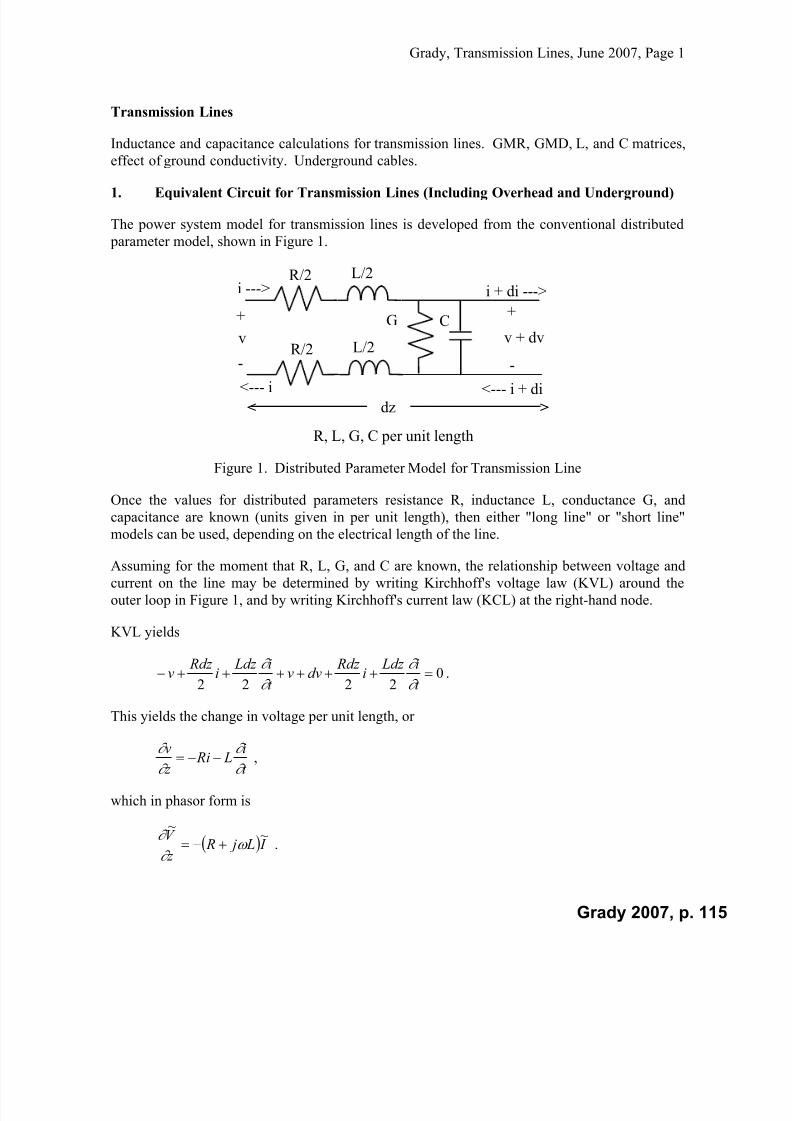
1. Equivalent Circuit for Transmission Lines (Including Overhead and Underground)
The power system model for transmission lines is developed from the conventional distributed
parameter model, shown in Figure 1.
+
-
v
R/2 L/2
G C
R/2 L/2
i --->
<--- i
+
-
v + dv
i + di --->
<--- i + di
R, L, G, C per unit length
< >dz
Figure 1. Distributed Parameter Model for Transmission Line
Once the values for distributed parameters resistance R, inductance L, conductance G, and
capacitance are known (units given in per unit length), then either "long line" or "short line"
models can be used, depending on the electrical length of the line.
Assuming for the moment that R, L, G, and C are known, the relationship between voltage andcurrent on the line may be determined by writing Kirchhoff's voltage law (KVL) around the
outer loop in Figure 1, and by writing Kirchhoff's current law (KCL) at the right-hand node.
KVL yields
02222
t
i Ldz i
Rdz dvv
t
i Ldz i
Rdz v
.
This yields the change in voltage per unit length, or
t i L Ri
z v
,
which in phasor form is
I L j R z
V ~~
.
Grady 2007, p. 115

7/22/2019 Fundamentals Grady Notes June 2007 Print
http://slidepdf.com/reader/full/fundamentals-grady-notes-june-2007-print 116/388
Grady, Transmission Lines, June 2007, Page 2
KCL at the right-hand node yields
0
t
dvvCdz dvvGdz diii
.
If dv is small, then the above formula can be approximated as
t
vCdz vGdz di
, or
t
vC Gv
z
i
, which in phasor form is
V C jG z
I ~~
.
Taking the partial derivative of the voltage phasor equation with respect to z yields
z
I
L j R z
V
~~
2
2
.
Combining the two above equations yields
V V C jG L j R z
V ~~~
2
2
2
, where jC jG L j R , and
where , , and are the propagation, attenuation, and phase constants, respectively.
The solution for V ~
is
z z Be Ae z V )(~ .
A similar procedure for solving I ~
yields
o
z z
Z
Be Ae z I
)(
~ ,
where the characteristic or "surge" impedance o Z is defined as
C jG
L j R Z o
.
Constants A and B must be found from the boundary conditions of the problem. This is usually
accomplished by considering the terminal conditions of a transmission line segment that is d
meters long, as shown in Figure 2.
Grady 2007, p. 116

7/22/2019 Fundamentals Grady Notes June 2007 Print
http://slidepdf.com/reader/full/fundamentals-grady-notes-june-2007-print 117/388
Grady, Transmission Lines, June 2007, Page 3
d< >
+
-
+
-
Vs Vr
Is ---> Ir --->
<--- Is <--- Ir
Sending End Receiving End
Transmission
Line Segment
z = 0z = -d
Figure 2. Transmission Line Segment
In order to solve for constants A and B, the voltage and current on the receiving end is assumed
to be known so that a relation between the voltages and currents on both sending and receiving
ends may be developed.
Substituting z = 0 into the equations for the voltage and current (at the receiving end) yields
o R R
Z
B A I B AV
~
,~
.
Solving for A and B yields
2
~
,2
~ Ro R Ro R I Z V
B I Z V
A
.
Substituting into the )(~
z V and )(~
z I equations yields
d I Z d V V R RS sinh~
cosh~~
0 ,
d I d Z
V I R
o
RS cosh
~sinh
~~
.
A pi equivalent model for the transmission line segment can now be found, in a similar manner
as it was for the off-nominal transformer. The results are given in Figure 3.
Grady 2007, p. 117
7/22/2019 Fundamentals Grady Notes June 2007 Print
http://slidepdf.com/reader/full/fundamentals-grady-notes-june-2007-print 118/388
Grady, Transmission Lines, June 2007, Page 4
d< >
+
-
+
-
Vs Vr
Is ---> Ir --->
<--- Is <--- Ir
Sending End Receiving End
z = 0z = -d
Ysr
Ys Yr
o RS
Z
d
Y Y
2
tanh
, d Z
Y o
SR sinh
1 ,
C jG
L j R Z o
, C jG L j R
R, L, G, C per unit length
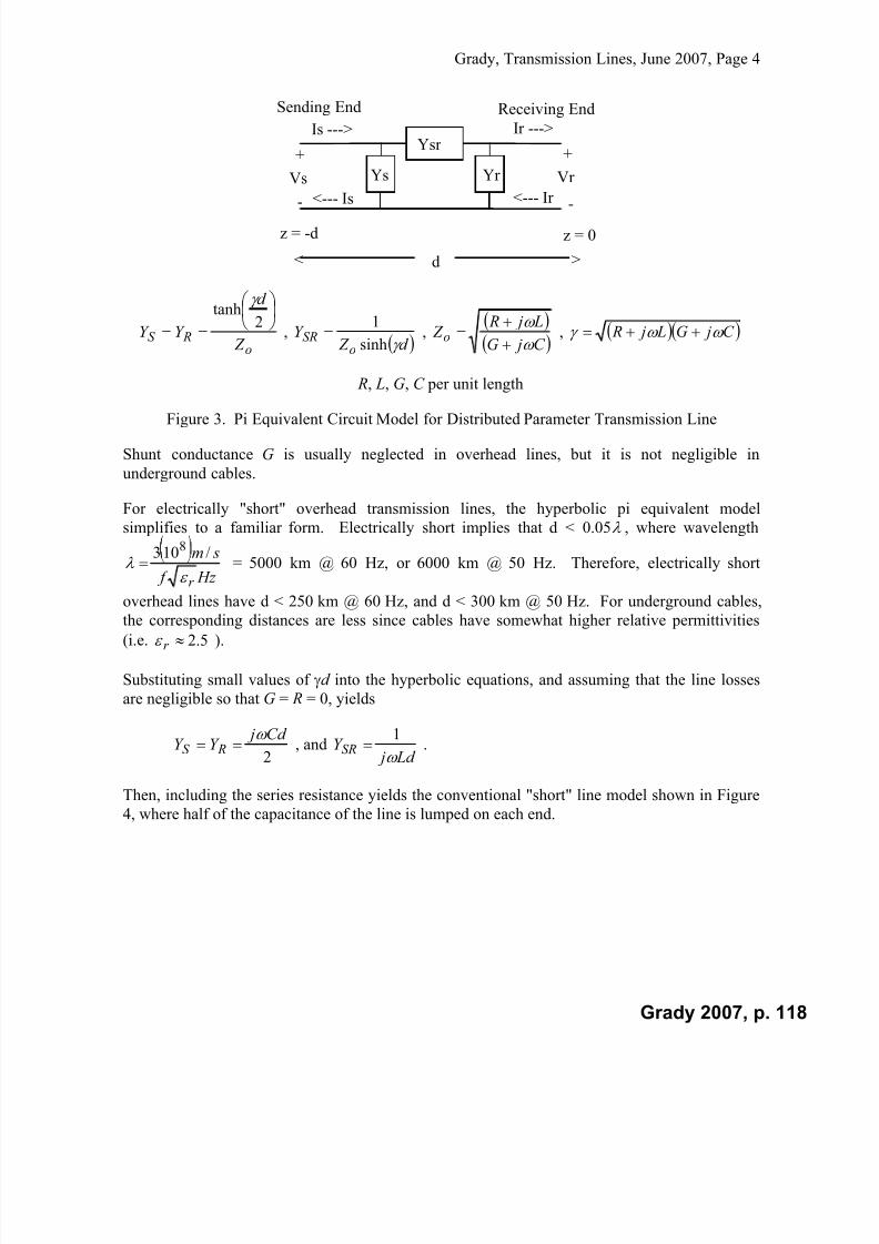
Figure 3. Pi Equivalent Circuit Model for Distributed Parameter Transmission Line
Shunt conductance G is usually neglected in overhead lines, but it is not negligible in
underground cables.
For electrically "short" overhead transmission lines, the hyperbolic pi equivalent model
simplifies to a familiar form. Electrically short implies that d < 0.05 , where wavelength
Hz f
sm
r
/103 8
= 5000 km @ 60 Hz, or 6000 km @ 50 Hz. Therefore, electrically short
overhead lines have d < 250 km @ 60 Hz, and d < 300 km @ 50 Hz. For underground cables,
the corresponding distances are less since cables have somewhat higher relative permittivities(i.e. 5.2r ).
Substituting small values of d into the hyperbolic equations, and assuming that the line losses
are negligible so that G = R = 0, yields
2
Cd jY Y RS
, and
Ld jY SR
1 .
Then, including the series resistance yields the conventional "short" line model shown in Figure
4, where half of the capacitance of the line is lumped on each end.
Grady 2007, p. 118

7/22/2019 Fundamentals Grady Notes June 2007 Print
http://slidepdf.com/reader/full/fundamentals-grady-notes-june-2007-print 119/388
Grady, Transmission Lines, June 2007, Page 5
< >d
Cd
2
Cd
2
Rd Ld
R, L, C per unit length
Figure 4. Standard Short Line Pi Equivalent Model for a Transmission Line
2. Capacitance of Overhead Transmission Lines
Overhead transmission lines consist of wires that are parallel to the surface of the earth. To
determine the capacitance of a transmission line, first consider the capacitance of a single wire
over the earth. Wires over the earth are typically modeled as line charges l Coulombs permeter of length, and the relationship between the applied voltage and the line charge is the
capacitance.
A line charge in space has a radially outward electric field described as
r o
l ar
q E ˆ
2 Volts per meter .
This electric field causes a voltage drop between two points at distances r = a and r = b away
from the line charge. The voltage is found by integrating electric field, or
a
bqar E V
o
l r
br
ar
ab ln2
ˆ
V.
If the wire is above the earth, it is customary to treat the earth's surface as a perfect conducting
plane, which can be modeled as an equivalent image line charge l q lying at an equal distance
below the surface, as shown in Figure 5.
Grady 2007, p. 119

7/22/2019 Fundamentals Grady Notes June 2007 Print
http://slidepdf.com/reader/full/fundamentals-grady-notes-june-2007-print 120/388
Grady, Transmission Lines, June 2007, Page 6
Surface of Earth
h
a
b
ai bi
A
Bh
Conductor with radius r, modeled electricallyas a line charge ql at the center
Image conductor, at an equal distance below
the Earth, and with negative line charge -ql
Figure 5. Line Charge l q at Center of Conductor Located h Meters Above the Earth
From superposition, the voltage difference between points A and B is
bia
aibq
ai
bi
a
bqa E a E V
o
l
o
l r
bir
air
ir
br
ar
ab ln2
lnln2
ˆˆ
.
If point B lies on the earth's surface, then from symmetry, b = bi, and the voltage of point A with
respect to ground becomes
a
aiqV
o
l ag ln
2 .
The voltage at the surface of the wire determines the wire's capacitance. This voltage is found
by moving point A to the wire's surface, corresponding to setting a = r , so that
r
hqV
o
l rg
2ln
2 for h >> r .
The exact expression, which accounts for the fact that the equivalent line charge drops slightly
below the center of the wire, but still remains within the wire, is
r
r hhqV
o
l rg
22
ln2
.
Grady 2007, p. 120

7/22/2019 Fundamentals Grady Notes June 2007 Print
http://slidepdf.com/reader/full/fundamentals-grady-notes-june-2007-print 121/388
Grady, Transmission Lines, June 2007, Page 7
The capacitance of the wire is defined asrg
l
V C
which, using the approximate voltage
formula above, becomes
r
hC o
2ln
2
Farads per meter of length.
When several conductors are present, then the capacitance of the configuration must be given in
matrix form. Consider phase a-b-c wires above the earth, as shown in Figure 6.
a
ai
b
bi
c
ci
Daai
Dabi
Daci
Dab
Dac
Surface of Earth
Three Conductors Represented by Their Equivalent Line Charges
Images
Conductor radii ra, rb, rc
Figure 6. Three Conductors Above the Earth
Superposing the contributions from all three line charges and their images, the voltage at the
surface of conductor a is given by
ac
acic
ab
abib
a
aaia
oag
D
Dq
D
Dq
r
DqV lnlnln
2
1
.
The voltages for all three conductors can be written in generalized matrix form as
c
b
a
cccbca
bcbbba
acabaa
ocg
bg
ag
q
p p p
p p p p p p
V
V V
2
1 , or abcabc
oabc Q P V
2
1 ,
where
Grady 2007, p. 121

7/22/2019 Fundamentals Grady Notes June 2007 Print
http://slidepdf.com/reader/full/fundamentals-grady-notes-june-2007-print 122/388
Grady, Transmission Lines, June 2007, Page 8
a
aaiaa
r
D p ln ,
ab
abiab
D
D p ln , etc., and
ar is the radius of conductor a,
aai D is the distance from conductor a to its own image (i.e. twice the height of
conductor a above ground),
ab D is the distance from conductor a to conductor b,
baiabi D D is the distance between conductor a and the image of conductor b (which
is the same as the distance between conductor b and the image of
conductor a), etc.
A Matrix Approach for Finding C
From the definition of capacitance, CV Q , then the capacitance matrix can be obtained via
inversion, or
12
abcoabc P C .
If ground wires are present, the dimension of the problem increases proportionally. For example,
in a three-phase system with two ground wires, the dimension of the P matrix is 5 x 5. However,
given the fact that the line-to-ground voltage of the ground wires is zero, equivalent 3 x 3 P and
C matrices can be found by using matrix partitioning and a process known as Kron reduction.
First, write the V = PQ equation as follows:
w
v
c
b
a
vwabcvw
vwabcabc
o
wg
vg
cg
bg
ag
q
q
q
q
q
P P
P P
V
V
V
V
V
)2x2(|)3x2(
)2x3(|)3x3(
2
1
0
0 ,
,
,
or
vw
abc
vwabcvw
vwabcabc
ovw
abc
Q
Q
P P
P P
V
V
,
,
2
1
,
where subscripts v and w refer to ground wires w and v, and where the individual P matrices are
formed as before. Since the ground wires have zero potential, then
Grady 2007, p. 122
7/22/2019 Fundamentals Grady Notes June 2007 Print
http://slidepdf.com/reader/full/fundamentals-grady-notes-june-2007-print 123/388
Grady, Transmission Lines, June 2007, Page 9
vwvwabcabcvwo
Q P Q P
,
2
1
0
0
,
so that
abcabcvwvwvw Q P P Q ,1 .
Substituting into the abcV equation above, and combining terms, yields
abcabcvwvwvwabcabco
abcabcvwvwvwabcabcabco
abc Q P P P P Q P P P Q P V ,1
,,1
,2
1
2
1
,
or
abcabcoabc
Q P V '
2
1
, so that
abcabcabc V C Q ' , where 1'' 2
abcoabc P C .
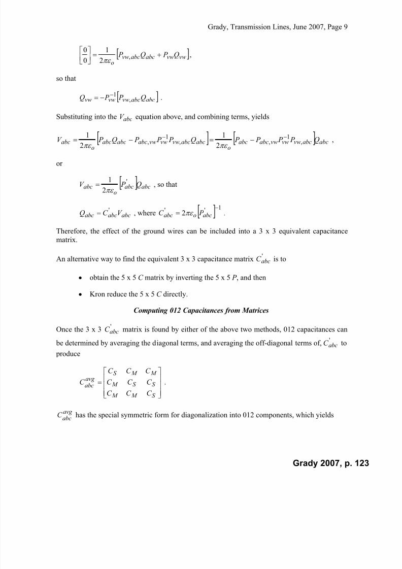
Therefore, the effect of the ground wires can be included into a 3 x 3 equivalent capacitance
matrix.
An alternative way to find the equivalent 3 x 3 capacitance matrix 'abcC is to
obtain the 5 x 5 C matrix by inverting the 5 x 5 P , and then
Kron reduce the 5 x 5 C directly.
Computing 012 Capacitances from Matrices
Once the 3 x 3 'abcC matrix is found by either of the above two methods, 012 capacitances can
be determined by averaging the diagonal terms, and averaging the off-diagonal terms of, 'abcC to
produce
S M M
S S M
M M S
avg abc
C C C
C C C
C C C
C .
avg abc
C has the special symmetric form for diagonalization into 012 components, which yields
Grady 2007, p. 123

7/22/2019 Fundamentals Grady Notes June 2007 Print
http://slidepdf.com/reader/full/fundamentals-grady-notes-june-2007-print 124/388
Grady, Transmission Lines, June 2007, Page 10
M S
M S
M S avg
C C
C C
C C
C
00
00
002
012 .
The Approximate Formulas for 012 Capacitances
Asymmetries in transmission lines prevent the P and C matrices from having the special form
that allows their diagonalization into decoupled positive, negative, and zero sequence
impedances. Transposition of conductors can be used to nearly achieve the special symmetric
form and, hence, improve the level of decoupling. Conductors are transposed so that each one
occupies each phase position for one-third of the lines total distance. An example is given below
in Figure 7, where the radii of all three phases are assumed to be identical.
a b c a cthen then
then then
bthen
b a c
b c a c a b c b a
where each configuration occupies one-sixth of the total distance
Figure 7. Transposition of A-B-C Phase Conductors
For this mode of construction, the average P matrix (or Kron reduced P matrix if ground wires
are present) has the following form:
cc
acaa
bcabbb
bb
bccc
abacaa
cc
bcbb
acabaaavg abc
p
p p
p p p
p
p p
p p p
p
p p
p p p
P 6
1
6
1
6
1
aa
abbb
acbccc
aa
accc
abbcbb
bb
abaa
bcaccc
p
p p
p p p
p
p p
p p p
p
p p
p p p
6
1
6
1 ,
where the individual p terms are described previously. Note that these individual P matrices aresymmetric, since baabbaab p p D D , , etc. Since the sum of natural logarithms is the same
as the logarithm of the product, P becomes
S M M
M S M
M M S avg
abc
p p p
p p p
p p p
P ,
Grady 2007, p. 124

7/22/2019 Fundamentals Grady Notes June 2007 Print
http://slidepdf.com/reader/full/fundamentals-grady-notes-june-2007-print 125/388
Grady, Transmission Lines, June 2007, Page 11
where
3
3
ln3 cba
ccibbiaaiccbbaa s
r r r
D D D P P P p
,
and
3
3
ln3 bcacab
bciaciabibcacabM
D D D
D D D P P P p
.
Since avg
abc P has the special property for diagonalization in symmetrical components, then
transforming it yields
M S
M S
M S avg
p p p p
p p
p p
p
P 00
00
002
0000
00
2
1
0
012 ,
where
33
33
3
3
3
3
lnlnlnbciaciabicba
bcacabccibbiaai
bcacab
bciaciabi
cba
ccibbiaaiM s
D D Dr r r
D D D D D D
D D D
D D D
r r r
D D D p p .
Inverting avg
P 012
and multiplying by o 2 yields the corresponding 012 capacitance matrix
M S
M S
M S
ooavg
p p
p p
p p
p
p
p
C
C
C
C
100
01
0
002
1
2
100
01
0
001
2
00
00
00
2
1
0
2
1
0
012 .
When the a-b-c conductors are closer to each other than they are to the ground, then
bciaciabiccibbiaai D D D D D D ,
yielding the conventional approximation
2,1
2,1
3
3
21 lnlnGMR
GMD
r r r
D D D p p p p
cba
bcacabM S ,
Grady 2007, p. 125
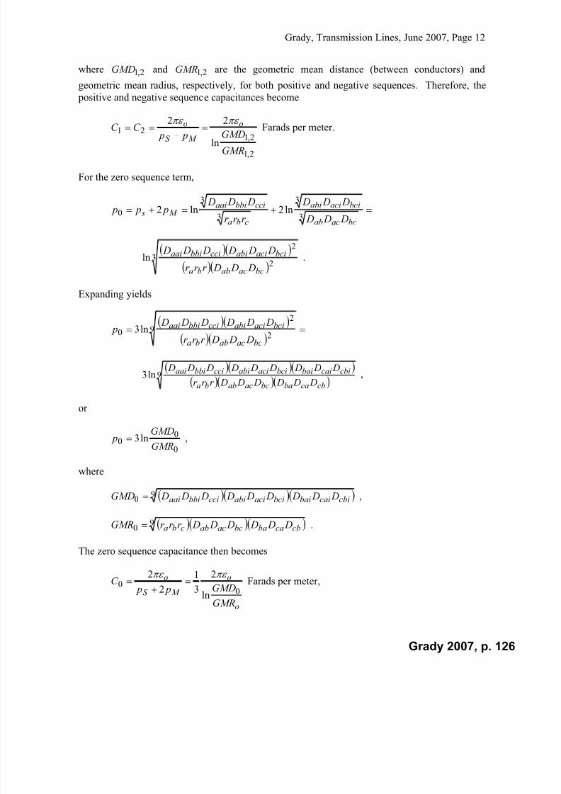
7/22/2019 Fundamentals Grady Notes June 2007 Print
http://slidepdf.com/reader/full/fundamentals-grady-notes-june-2007-print 126/388
Grady, Transmission Lines, June 2007, Page 12
where 2,1GMD and 2,1GMR are the geometric mean distance (between conductors) and
geometric mean radius, respectively, for both positive and negative sequences. Therefore, the
positive and negative sequence capacitances become
2,1
2,121ln
22
GMR
GMD p pC C
o
M S
o
Farads per meter.
For the zero sequence term,
3
3
3
3
0 ln2ln2bcacab
bciaciabi
cba
ccibbiaaiM s
D D D
D D D
r r r
D D D p p p
3
2
2
ln
bcacabba
bciaciabiccibbiaai
D D Dr r r
D D D D D D .
Expanding yields
9
2
2
0 ln3
bcacabba
bciaciabiccibbiaai
D D Dr r r
D D D D D D p
9ln3cbcababcacabba
cbicaibaibciaciabiccibbiaai
D D D D D Dr r r
D D D D D D D D D ,
or
0
00 ln3
GMR
GMD p ,
where
90 cbicaibaibciaciabiccibbiaai D D D D D D D D DGMD ,
9
0 cbcababcacabcba D D D D D Dr r r GMR .
The zero sequence capacitance then becomes
o
o
M S
o
GMR
GMD p pC
00
ln
2
3
1
2
2
Farads per meter,
Grady 2007, p. 126
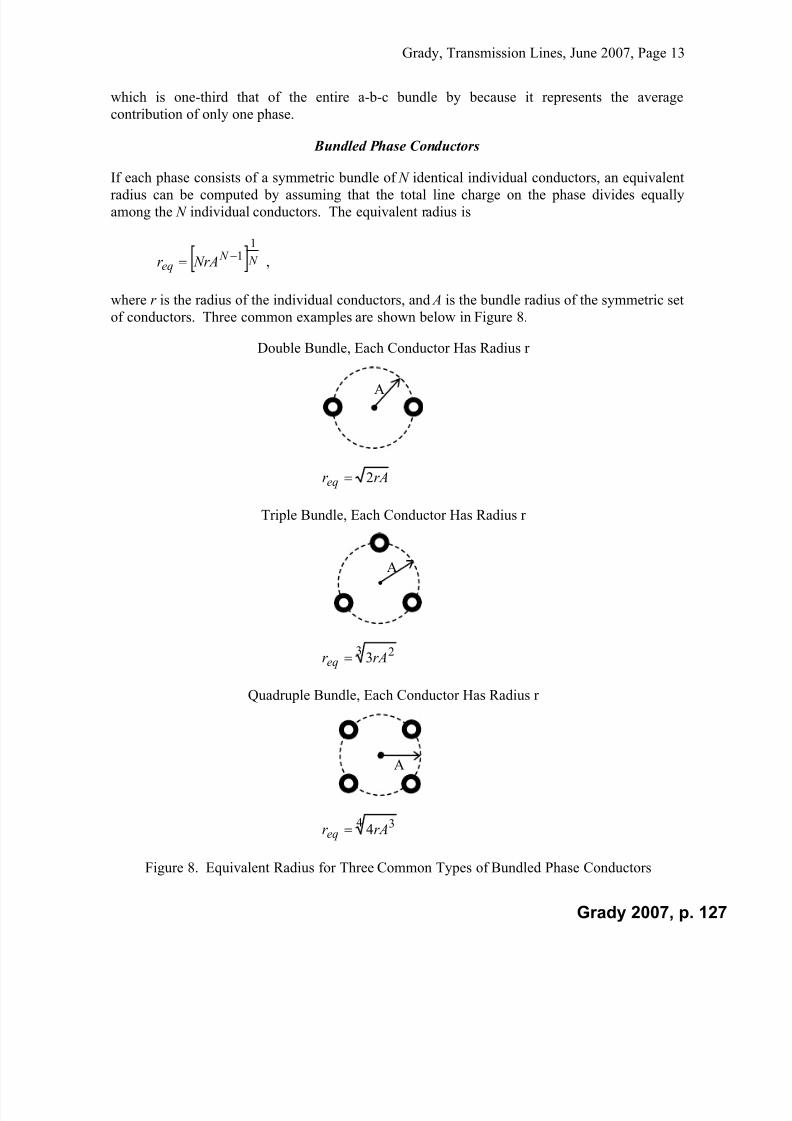
7/22/2019 Fundamentals Grady Notes June 2007 Print
http://slidepdf.com/reader/full/fundamentals-grady-notes-june-2007-print 127/388
Grady, Transmission Lines, June 2007, Page 13
which is one-third that of the entire a-b-c bundle by because it represents the average
contribution of only one phase.
Bundled Phase Conductors
If each phase consists of a symmetric bundle of N identical individual conductors, an equivalent
radius can be computed by assuming that the total line charge on the phase divides equally
among the N individual conductors. The equivalent radius is
N N eq NrAr
11 ,
where r is the radius of the individual conductors, and A is the bundle radius of the symmetric set
of conductors. Three common examples are shown below in Figure 8.
Double Bundle, Each Conductor Has Radius r
A
rAr eq 2
Triple Bundle, Each Conductor Has Radius r
A
3 23rAr eq
Quadruple Bundle, Each Conductor Has Radius r
A
4 34rAr eq
Figure 8. Equivalent Radius for Three Common Types of Bundled Phase Conductors
Grady 2007, p. 127
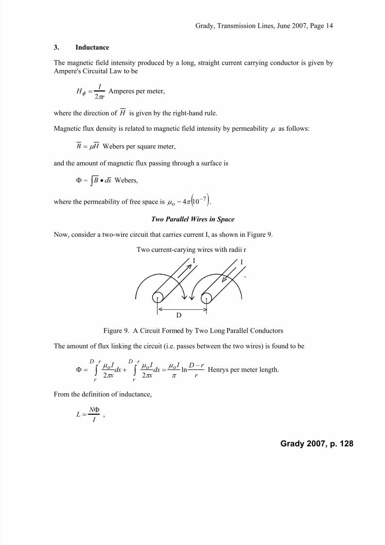
7/22/2019 Fundamentals Grady Notes June 2007 Print
http://slidepdf.com/reader/full/fundamentals-grady-notes-june-2007-print 128/388
Grady, Transmission Lines, June 2007, Page 14
3. Inductance
The magnetic field intensity produced by a long, straight current carrying conductor is given by
Ampere's Circuital Law to be
r
I H
2 Amperes per meter,
where the direction of H is given by the right-hand rule.
Magnetic flux density is related to magnetic field intensity by permeability as follows:
H B Webers per square meter,
and the amount of magnetic flux passing through a surface is
sd B Webers,
where the permeability of free space is 7104 o .
Two Parallel Wires in Space
Now, consider a two-wire circuit that carries current I, as shown in Figure 9.
I I
Two current-carying wires with radii r
D< >
Figure 9. A Circuit Formed by Two Long Parallel Conductors
The amount of flux linking the circuit (i.e. passes between the two wires) is found to be
r
r D I dx
x
I dx
x
I or D
r
or D
r
o ln22
Henrys per meter length.
From the definition of inductance,
I
N L
,
Grady 2007, p. 128

7/22/2019 Fundamentals Grady Notes June 2007 Print
http://slidepdf.com/reader/full/fundamentals-grady-notes-june-2007-print 129/388
Grady, Transmission Lines, June 2007, Page 15
where in this case N = 1, and where N >> r , the inductance of the two-wire pair becomes
r
D L o ln
Henrys per meter length.
A round wire also has an internal inductance, which is separate from the external inductanceshown above. The internal inductance is shown in electromagnetics texts to be
8
int int L Henrys per meter length.
For most current-carrying conductors, oint so that int L = 0.05µH/m. Therefore, the total
inductance of the two-wire circuit is the external inductance plus twice the internal inductance of
each wire (i.e. current travels down and back), so that
4
14
1
lnlnln41ln
82ln
re
Der
Dr
Dr
D L oooootot
.
It is customary to define an effective radius
r rer eff 7788.04
1
,
and to write the total inductance in terms of it as
eff
otot
r D L ln
Henrys per meter length.
Wire Parallel to Earth’s Surface
For a single wire of radius r , located at height h above the earth, the effect of the earth can be
described by an image conductor, as it was for capacitance calculations. For a perfectly
conducting earth, the image conductor is located h meters below the surface, as shown in Figure
10.
Grady 2007, p. 129
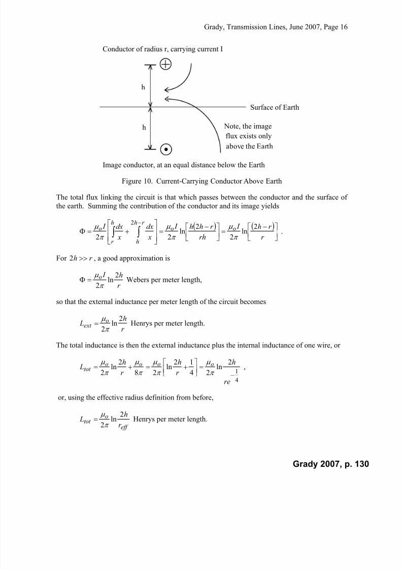
7/22/2019 Fundamentals Grady Notes June 2007 Print
http://slidepdf.com/reader/full/fundamentals-grady-notes-june-2007-print 130/388
Grady, Transmission Lines, June 2007, Page 16
Surface of Earth
h
h
Conductor of radius r, carrying current I
Note, the image
flux exists only
above the Earth
Image conductor, at an equal distance below the Earth
Figure 10. Current-Carrying Conductor Above Earth
The total flux linking the circuit is that which passes between the conductor and the surface of
the earth. Summing the contribution of the conductor and its image yields
r
r h I
rh
r hh I
x
dx
x
dx I ooh
r
r h
h
o 2ln
2
2ln
22
2
.
For 2h r , a good approximation is
r
h I o 2ln
2
Webers per meter length,
so that the external inductance per meter length of the circuit becomes
r
h L o
ext 2
ln2
Henrys per meter length.
The total inductance is then the external inductance plus the internal inductance of one wire, or
4
1
2ln
24
12ln
28
2ln
2
re
h
r
h
r
h L oooo
tot
,
or, using the effective radius definition from before,
eff
otot
r
h L
2ln
2
Henrys per meter length.
Grady 2007, p. 130
7/22/2019 Fundamentals Grady Notes June 2007 Print
http://slidepdf.com/reader/full/fundamentals-grady-notes-june-2007-print 131/388
Grady, Transmission Lines, June 2007, Page 17
Bundled Conductors
The bundled conductor equivalent radii presented earlier apply for inductance as well as for
capacitance. The question now is “what is the internal inductance of a bundle?” For N bundled
conductors, the net internal inductance of a phase per meter must decrease as
N
1 because the
internal inductances are in parallel. Considering a bundle over the Earth, then
N
eq
o
eq
o
eq
oo
eq
otot
er
he
N r
h
N r
h
N r
h L
4
14
12
ln2
ln12
ln24
12ln
28
2ln
2
.
Factoring in the expression for the equivalent bundle radius eqr yields
N N eff
N N N N N N
eq A Nr A Nree NrAer
11
1
14
1
4
1114
1
Thus, eff r remains 4
1
re , no matter how many conductors are in the bundle.
The Three-Phase Case
For situations with multiples wires above the Earth, a matrix approach is needed. Consider thecapacitance example given in Figure 6, except this time compute the external inductances, rather
than capacitances. As far as the voltage (with respect to ground) of one of the a-b-c phases is
concerned, the important flux is that which passes between the conductor and the Earth's surface.
For example, the flux "linking" phase a will be produced by six currents: phase a current and its
image, phase b current and its image, and phase c current and its image, and so on. Figure 11 is
useful in visualizing the contribution of flux “linking” phase a that is caused by the current in
phase b (and its image).
Grady 2007, p. 131
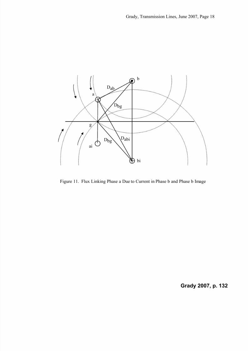
7/22/2019 Fundamentals Grady Notes June 2007 Print
http://slidepdf.com/reader/full/fundamentals-grady-notes-june-2007-print 132/388
Grady, Transmission Lines, June 2007, Page 18
a
ai
b
bi
Dab
D bg
D bgDabi
g
Figure 11. Flux Linking Phase a Due to Current in Phase b and Phase b Image
Grady 2007, p. 132
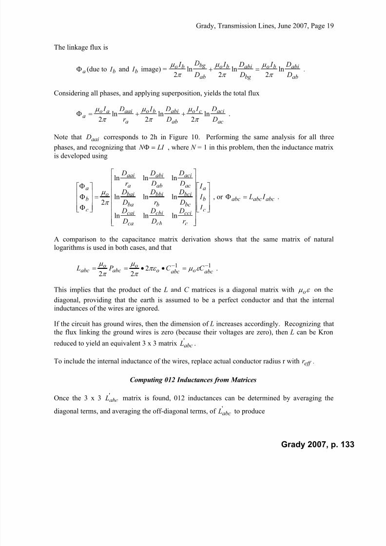
7/22/2019 Fundamentals Grady Notes June 2007 Print
http://slidepdf.com/reader/full/fundamentals-grady-notes-june-2007-print 133/388
7/22/2019 Fundamentals Grady Notes June 2007 Print
http://slidepdf.com/reader/full/fundamentals-grady-notes-june-2007-print 134/388
Grady, Transmission Lines, June 2007, Page 20
S M M
S S M
M M S avg abc
L L L
L L L
L L L
L ,
so that
M S
M S
M S avg
L L
L L
L L
L
00
00
002
012 .
The Approximate Formulas for 012 Inductancess
Because of the similarity to the capacitance problem, the same rules for eliminating ground
wires, for transposition, and for bundling conductors apply. Likewise, approximate formulas for
the positive, negative, and zero sequence inductances can be developed, and these formulas are
2,1
2,121 ln
2 GMR
GMD L L o
,
and
0
00 ln
23
GMR
GMD L o
.
It is important to note that the GMD and GMR terms for inductance differ from those of
capacitance in two ways:
1. GMR calculations for inductance calculations should be made with 4
1
rer eff .
2. GMD distances for inductance calculations should include the equivalent complex depth for
modeling finite conductivity earth (explained in the next section). This effect is ignored in
capacitance calculations because the surface of the Earth is nominally at zero potential.
The Complex Depth Method for Modeling Imperfect Earth
The effect of the Earth's non-infinite conductivity should be included when computinginductances, especially zero sequence inductances. Because the Earth is not a perfect conductor,
the image current does not actually flow on the surface of the Earth, but rather through a cross-
section. The higher the conductivity, the narrower the cross-section.
The simplest method to account for finite conductivity is via a complex depth cd , where the
equivalent earth surface is assumed to be an additional cd meters below the actual earth surface.
Grady 2007, p. 134

7/22/2019 Fundamentals Grady Notes June 2007 Print
http://slidepdf.com/reader/full/fundamentals-grady-notes-june-2007-print 135/388
Grady, Transmission Lines, June 2007, Page 21
Using complex depth, if a conductor is d meters above earth, its image is cd d 2 meters
below the conductor.
The complex depth cd is related to resistive skin depth by
jd c
1
= o45
2
=
22
j ,
where
f
1 .
At f = 60 Hz andm
1
01.0 (typical for limestone), the skin depth is 650 meters, so that
2
650
2
650 jd c = 325 – j325 m.
Skin depth in typical soils for 50 - 60 Hz varies from 500 to 2000 meters. The effect on
positive/negative sequence inductances is not great, but the effect on zero sequence inductances
is quite significant.
Since cd is a frequency-dependent complex number, the self- and image-distance terms are
complex, their natural logarithms are complex, and the L matrix contains complex numbers. The
questions now are “how to take the natural log of a complex number and how to interpret the
results?”
Begin with the natural log of a complex number je z z , which is
Earth’s Surface
d c
Equivalent Earth’s Surface
d c
d
d
Grady 2007, p. 135
7/22/2019 Fundamentals Grady Notes June 2007 Print
http://slidepdf.com/reader/full/fundamentals-grady-notes-june-2007-print 136/388
Grady, Transmission Lines, June 2007, Page 22
j z e z z j ln)ln(ln)ln( , in radians.
Thus, for example, 4
325ln)325325ln(
j j = 5.78 – j0.785.
To be consistent with the perfect Earth case (i.e., 0, ), the real part of the natural
logarithm must produce the inductive term. Then, the imaginary term yields the resistance of the
Earth’s current path, which must be added to the series resistances of the overhead conductors.
In matrix form, the calculations are made accoding to
c
cci
bc
bci
b
bbi
ac
aci
ab
abi
a
aai
oabcabc
r Dcomplex
D
Dcomplex
r
Dcomplex
D
Dcomplex
D
Dcomplex
r
Dcomplex
j L j R
ln
lnln
lnlnln
2)()(
,
where complex depth cd is included in the D terms. Because of the j multiplier, the real
terms become positive, frequency-dependent resistances that account for the losses in the Earth.
Off-diagonal resistances account for the fact that currents in neighboring phases contribute to the
total voltage drop along the Earth, per meter, as seen by any given phase. The imaginary terms
are inductive reactances.
4. Electric Field at Surface of Overhead Conductors
Ignoring all other charges, the electric field at a conductor’s surface can be approximated by
r
q E
or
2 ,
where r is the radius. For overhead conductors, this is a reasonable approximation because the
neighboring line charges are relatively far away. It is always important to keep the peak electric
field at a conductor’s surface below 30kV/cm to avoid excessive corono losses.
Going beyond the above approximation, the Markt-Mengele method provides a detailed
procedure for calculating the maximum peak subconductor surface electric field intensity for
three-phase lines with identical phase bundles. Each bundle has N symmetric subconductors ofradius r . The bundle radius is A. The procedure is
1. Treat each phase bundle as a single conductor with equivalent radius
N N eq NrAr /11 .
Grady 2007, p. 136

7/22/2019 Fundamentals Grady Notes June 2007 Print
http://slidepdf.com/reader/full/fundamentals-grady-notes-june-2007-print 137/388
Grady, Transmission Lines, June 2007, Page 23
2. Find the C(N x N) matrix, including ground wires, using average conductor heights above
ground. Kron reduce C(N x N) to C(3 x 3). Select the phase bundle that will have the
greatest peak line charge value ( lpeak q ) during a 60Hz cycle by successively placing
maximum line-to-ground voltage V max on one phase, and – V max/2 on each of the other
two phases. Usually, the phase with the largest diagonal term in C(3 by 3) will have the
greatest lpeak q .
3. Assuming equal charge division on the phase bundle identified in Step 2, ignore
equivalent line charge displacement, and calculate the average peak subconductor surface
electric field intensity using
r N
q E
o
lpeak peak avg
2
1,
4. Take into account equivalent line charge displacement, and calculate the maximum peak
subconductor surface electric field intensity using
A
r N E E peak avg peak )1(1,max, .
5. Resistance and Conductance
The resistance of conductors is frequency dependent because of the resistive skin effect.
Usually, however, this phenomenon is small for 50 - 60 Hz. Conductor resistances are readily
obtained from tables, in the proper units of Ohms per meter length, and these values, added to
the equivalent-earth resistances from the previous section, to yield the R used in the transmission
line model.
Conductance G is very small for overhead transmission lines and can be ignored.
6. Underground Cables
Underground cables are transmission lines, and the model previously presented applies.
Capacitance C tends to be much larger than for overhead lines, and conductance G should not be
ignored.
For single-phase and three-phase cables, the capacitances and inductances per phase per meter
length are
a
bC r o
ln
2 Farads per meter length,
and
Grady 2007, p. 137

7/22/2019 Fundamentals Grady Notes June 2007 Print
http://slidepdf.com/reader/full/fundamentals-grady-notes-june-2007-print 138/388
Grady, Transmission Lines, June 2007, Page 24
a
b L o ln
2
Henrys per meter length,
where b and a are the outer and inner radii of the coaxial cylinders. In power cables,a
b is
typically e (i.e., 2.7183) so that the voltage rating is maximized for a given diameter.
For most dielectrics, relative permittivity 5.20.2 r . For three-phase situations, it is
common to assume that the positive, negative, and zero sequence inductances and capacitances
equal the above expressions. If the conductivity of the dielectric is known, conductance G can
be calculated using
C G Mhos per meter length.
Grady 2007, p. 138
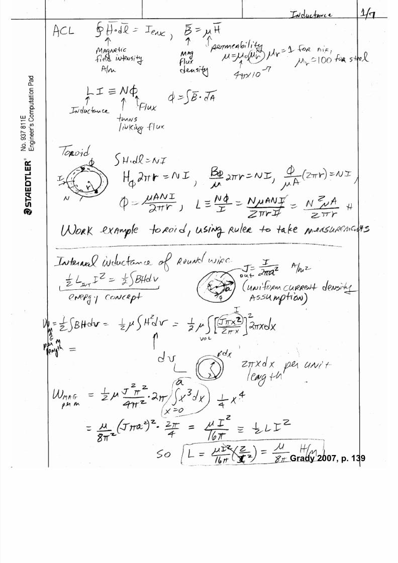
7/22/2019 Fundamentals Grady Notes June 2007 Print
http://slidepdf.com/reader/full/fundamentals-grady-notes-june-2007-print 139/388
Grady 2007, p. 139

7/22/2019 Fundamentals Grady Notes June 2007 Print
http://slidepdf.com/reader/full/fundamentals-grady-notes-june-2007-print 140/388
Grady 2007, p. 140
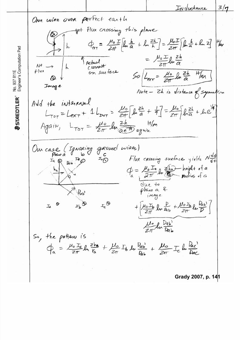
7/22/2019 Fundamentals Grady Notes June 2007 Print
http://slidepdf.com/reader/full/fundamentals-grady-notes-june-2007-print 141/388
Grady 2007, p. 141

7/22/2019 Fundamentals Grady Notes June 2007 Print
http://slidepdf.com/reader/full/fundamentals-grady-notes-june-2007-print 142/388
Grady 2007, p. 142

7/22/2019 Fundamentals Grady Notes June 2007 Print
http://slidepdf.com/reader/full/fundamentals-grady-notes-june-2007-print 143/388
Grady 2007, p. 143

7/22/2019 Fundamentals Grady Notes June 2007 Print
http://slidepdf.com/reader/full/fundamentals-grady-notes-june-2007-print 144/388
Grady 2007, p. 144

7/22/2019 Fundamentals Grady Notes June 2007 Print
http://slidepdf.com/reader/full/fundamentals-grady-notes-june-2007-print 145/388
Grady 2007, p. 145
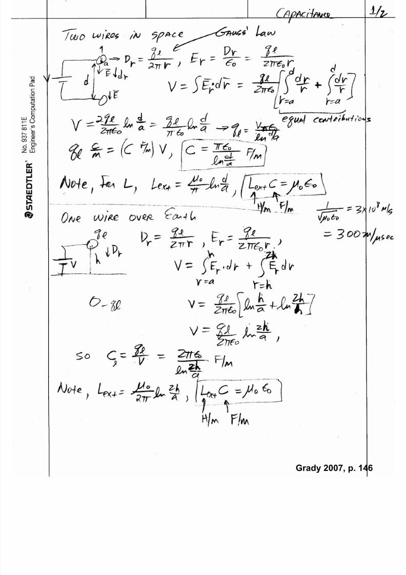
7/22/2019 Fundamentals Grady Notes June 2007 Print
http://slidepdf.com/reader/full/fundamentals-grady-notes-june-2007-print 146/388
Grady 2007, p. 146

7/22/2019 Fundamentals Grady Notes June 2007 Print
http://slidepdf.com/reader/full/fundamentals-grady-notes-june-2007-print 147/388
Grady 2007, p. 147

7/22/2019 Fundamentals Grady Notes June 2007 Print
http://slidepdf.com/reader/full/fundamentals-grady-notes-june-2007-print 148/388
Procedure for Computing Positive/Negative/Zero Sequence Line Constants for
Transmission Lines in Air
Page 1 of 6
POSITIVE/NEGATIVE SEQUENCE CALCULATIONS
Assumptions
Balanced, far from ground, ground wires ignored. Valid for identical single conductors per
phase, or for identical symmetric phase bundles with N conductors per phase and bundle radiusA.
Computation of positive/negative sequence capacitance
/
//
ln
2
C
o
GMR
GMDC
farads per meter,
where
3/ bcacab D D DGMD meters,
where bcacab D D D ,, are
distances between phase conductors if the line has one conductor per phase, or
distances between phase bundle centers if the line has symmetric phase bundles,
and where
/C GMR is the actual conductor radius r (in meters) if the line has one conductor per phase, or
N N C Ar N GMR 1
/
if the line has symmetric phase bundles.
Computation of positive/negative sequence inductance
/
// ln
2 L
o
GMR
GMD L
henrys per meter,
where /GMD is the same as for capacitance, and
for the single conductor case, / LGMR is the conductor gmr r (in meters), which takes
into account both stranding and the 4/1e adjustment for internal inductance. If gmr r is
not given, then assume 4/1 rer gmr , and
for bundled conductors, N N gmr L Ar N GMR 1
/
if the line has symmetric phase
bundles.
Grady 2007, p. 148
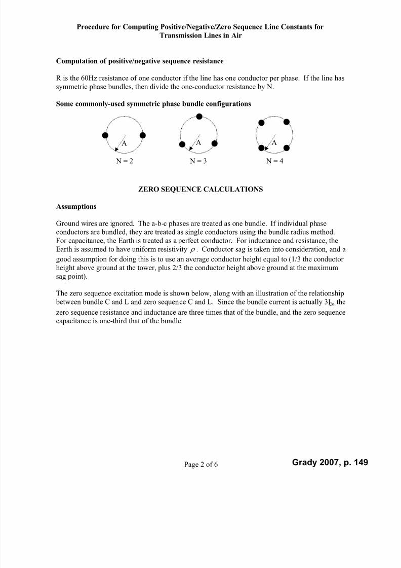
7/22/2019 Fundamentals Grady Notes June 2007 Print
http://slidepdf.com/reader/full/fundamentals-grady-notes-june-2007-print 149/388
Procedure for Computing Positive/Negative/Zero Sequence Line Constants for
Transmission Lines in Air
Page 2 of 6
Computation of positive/negative sequence resistance
R is the 60Hz resistance of one conductor if the line has one conductor per phase. If the line has
symmetric phase bundles, then divide the one-conductor resistance by N.
Some commonly-used symmetric phase bundle configurations
ZERO SEQUENCE CALCULATIONS
Assumptions
Ground wires are ignored. The a-b-c phases are treated as one bundle. If individual phaseconductors are bundled, they are treated as single conductors using the bundle radius method.
For capacitance, the Earth is treated as a perfect conductor. For inductance and resistance, the
Earth is assumed to have uniform resistivity . Conductor sag is taken into consideration, and a
good assumption for doing this is to use an average conductor height equal to (1/3 the conductor
height above ground at the tower, plus 2/3 the conductor height above ground at the maximum
sag point).
The zero sequence excitation mode is shown below, along with an illustration of the relationship
between bundle C and L and zero sequence C and L. Since the bundle current is actually 3Io, the
zero sequence resistance and inductance are three times that of the bundle, and the zero sequence
capacitance is one-third that of the bundle.
A A A
N = 2 N = 3 N = 4
Grady 2007, p. 149

7/22/2019 Fundamentals Grady Notes June 2007 Print
http://slidepdf.com/reader/full/fundamentals-grady-notes-june-2007-print 150/388
Procedure for Computing Positive/Negative/Zero Sequence Line Constants for
Transmission Lines in Air
Page 3 of 6
Computation of zero sequence capacitance
0
00
ln
2
3
1
C
C
o
GMR
GMDC
farads per meter,
where 0C GMD is the average height (with sag factored in) of the a-b-c bundle above perfect
Earth. 0C GMD is computed using
9222
0 ibc
iac
iab
iccibbiaaC D D D D D DGMD meters,
where iaa D is the distance from a to a-image, iab
D is the distance from a to b-image, and so
forth. The Earth is assumed to be a perfect conductor, so that the images are the same distance
below the Earth as are the conductors above the Earth. Also,
92223
/0 bcacabC C D D DGMRGMR meters,
where /C GMR , ab D , ac D , and bc D were described previously.
Computation of zero sequence inductance
00 ln
23
L
eo
GMR
D L
Henrys per meter,
+V
o –
Io
Io
Io 3Io
C bundle
+V
o –
Io
Io
Io 3Io
3Io
L bundle
+Vo
–
Io
Io
Io 3Io
Co Co Co
Io
+Vo
–
Io
Io 3Io
3Io Lo
Lo
Lo
Grady 2007, p. 150

7/22/2019 Fundamentals Grady Notes June 2007 Print
http://slidepdf.com/reader/full/fundamentals-grady-notes-june-2007-print 151/388
Procedure for Computing Positive/Negative/Zero Sequence Line Constants for
Transmission Lines in Air
Page 4 of 6
where f
De
4.658 meters (see Bergen), is the resistivity of the Earth (a good assumption
is 100-m), and f is the frequency (Hz). e D takes into account the fact that the Earth is
resistive and that zero sequence currents flow deep in the Earth. In most cases, e D is so large
that the actual height of the conductors makes no difference in the calculations. For example, for
60Hz and = 100-m, e D = 850m.
The geometric mean bundle radius is computed using
92223
/0 bcacab L L D D DGMRGMR meters,
where / LGMR , ab D , ac D , and bc D were shown previously.
Computation of zero sequence resistance
There are two components of zero sequence line resistance. First, the equivalent conductorresistance is the 60Hz resistance of one conductor if the line has one conductor per phase. If the
line has symmetric phase bundles with N conductors per bundle, then divide the one-conductor
resistance by N.
Second, the effect of resistive Earth is included by adding the following term to the conductorresistance:
f 7
10869.93
ohms per meter (see Bergen),
where the multiplier of three is needed to take into account the fact that all three zero sequence
currents flow through the Earth.
Electric Field at Surface of Overhead Conductors
Ignoring all other charges, the electric field at a conductor’s surface can be approximated by
r
q E
o
r
2
,
where r is the radius. For overhead conductors, this is a reasonable approximation because the
neighboring line charges are relatively far away. It is always important to keep the peak electric
field at a conductor’s surface below 30kV/cm to avoid excessive corono losses.
Going beyond the above approximation, the Markt-Mengele method provides a detailed
procedure for calculating the maximum peak subconductor surface electric field intensity forthree-phase lines with identical phase bundles. Each bundle has N symmetric subconductors of
radius r . The bundle radius is A. The procedure is
Grady 2007, p. 151

7/22/2019 Fundamentals Grady Notes June 2007 Print
http://slidepdf.com/reader/full/fundamentals-grady-notes-june-2007-print 152/388
Procedure for Computing Positive/Negative/Zero Sequence Line Constants for
Transmission Lines in Air
Page 5 of 6
1. Treat each phase bundle as a single conductor with equivalent radius
N N eq NrAr /11 .
2. Find theC(N x N)
matrix, including ground wires, using average conductor heights above
ground. Kron reduce C(N x N) to C(3 x 3). Select the phase bundle that will have the
greatest peak line charge value ( lpeak q ) during a 60Hz cycle by successively placing
maximum line-to-ground voltage V max on one phase, and – V max/2 on each of the other
two phases. Usually, the phase with the largest diagonal term in C(3 by 3) will have the
greatest lpeak q .
3. Assuming equal charge division on the phase bundle identified in Step 2, ignore
equivalent line charge displacement, and calculate the average peak subconductor surfaceelectric field intensity using
r N
q E
o
lpeak peak avg
2
1,
4. Take into account equivalent line charge displacement, and calculate the maximum peaksubconductor surface electric field intensity using
A
r N E E peak avg peak )1(1,max, .
Grady 2007, p. 152

7/22/2019 Fundamentals Grady Notes June 2007 Print
http://slidepdf.com/reader/full/fundamentals-grady-notes-june-2007-print 153/388
Procedure for Computing Positive/Negative/Zero Sequence Line Constants for
Transmission Lines in Air
Page 6 of 6
Practice Problem – a 345kV double-circuit configuration that is commonly used in Texas
Grady 2007, p. 153
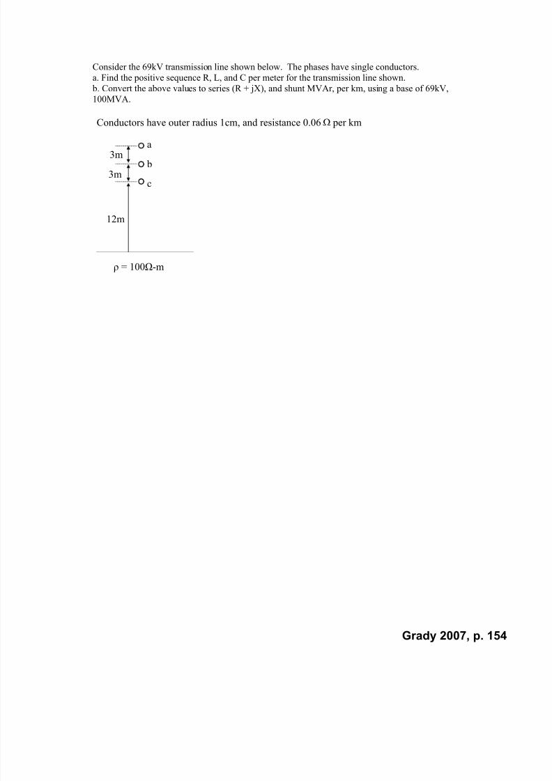
7/22/2019 Fundamentals Grady Notes June 2007 Print
http://slidepdf.com/reader/full/fundamentals-grady-notes-june-2007-print 154/388
Consider the 69kV transmission line shown below. The phases have single conductors.
a. Find the positive sequence R, L, and C per meter for the transmission line shown.
b. Convert the above values to series (R + jX), and shunt MVAr, per km, using a base of 69kV,
100MVA.
a
b
c
12m
3m
3m
= 100-m
Conductors have outer radius 1cm, and resistance 0.06 per km
Grady 2007, p. 154

7/22/2019 Fundamentals Grady Notes June 2007 Print
http://slidepdf.com/reader/full/fundamentals-grady-notes-june-2007-print 155/388

7/22/2019 Fundamentals Grady Notes June 2007 Print
http://slidepdf.com/reader/full/fundamentals-grady-notes-june-2007-print 156/388
Each phase of the 345kV transmission configuration shown has two bundled 795ACSR
conductors, separated by 45.7cm. The characteristics of a 795ACSR conductor are
r = 1.407cm, r gmr = 1.137cm,
R 60Hz = 0.0728/km.
The conversion from feet to meters is 3.281 feet per meter.
a. Find the positive/negative sequence C, L, and R permeter of length
b. Draw the corresponding pi-equivalent circuit, in ohms
@ 60Hz, for a 100km long line.
ft.
Grady 2007, p. 156
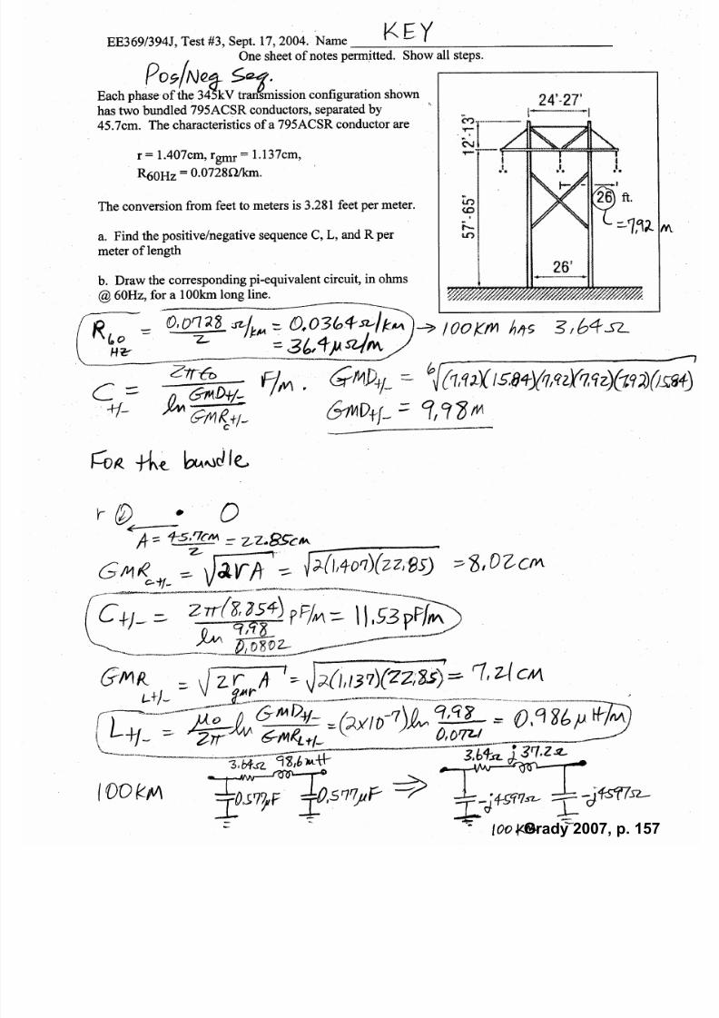
7/22/2019 Fundamentals Grady Notes June 2007 Print
http://slidepdf.com/reader/full/fundamentals-grady-notes-june-2007-print 157/388
Grady 2007, p. 157

7/22/2019 Fundamentals Grady Notes June 2007 Print
http://slidepdf.com/reader/full/fundamentals-grady-notes-june-2007-print 158/388
The a-b-c phase bundles of a three-phase, 345kV transmission line have the spacings and
average heights above Earth as shown. Each conductor has outer radius 1cm, and the twoconductors per phase are separated by 45cm. Ignoring ground wires, and making the “far from
Earth” assumption, compute the positive/negative sequence inductance and capacitance per
meter length (express your answer in µH/m and pF/m). Important - include the internal
inductance in the µH/m calculation.
20m
6m 6m
Grady 2007, p. 158
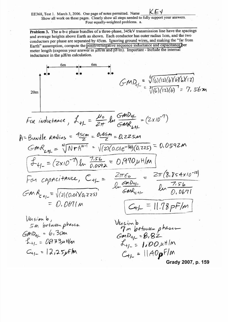
7/22/2019 Fundamentals Grady Notes June 2007 Print
http://slidepdf.com/reader/full/fundamentals-grady-notes-june-2007-print 159/388
Grady 2007, p. 159
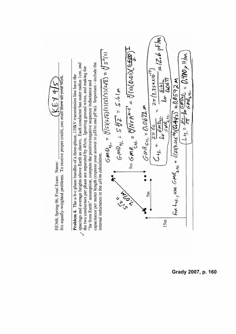
7/22/2019 Fundamentals Grady Notes June 2007 Print
http://slidepdf.com/reader/full/fundamentals-grady-notes-june-2007-print 160/388
Grady 2007, p. 160
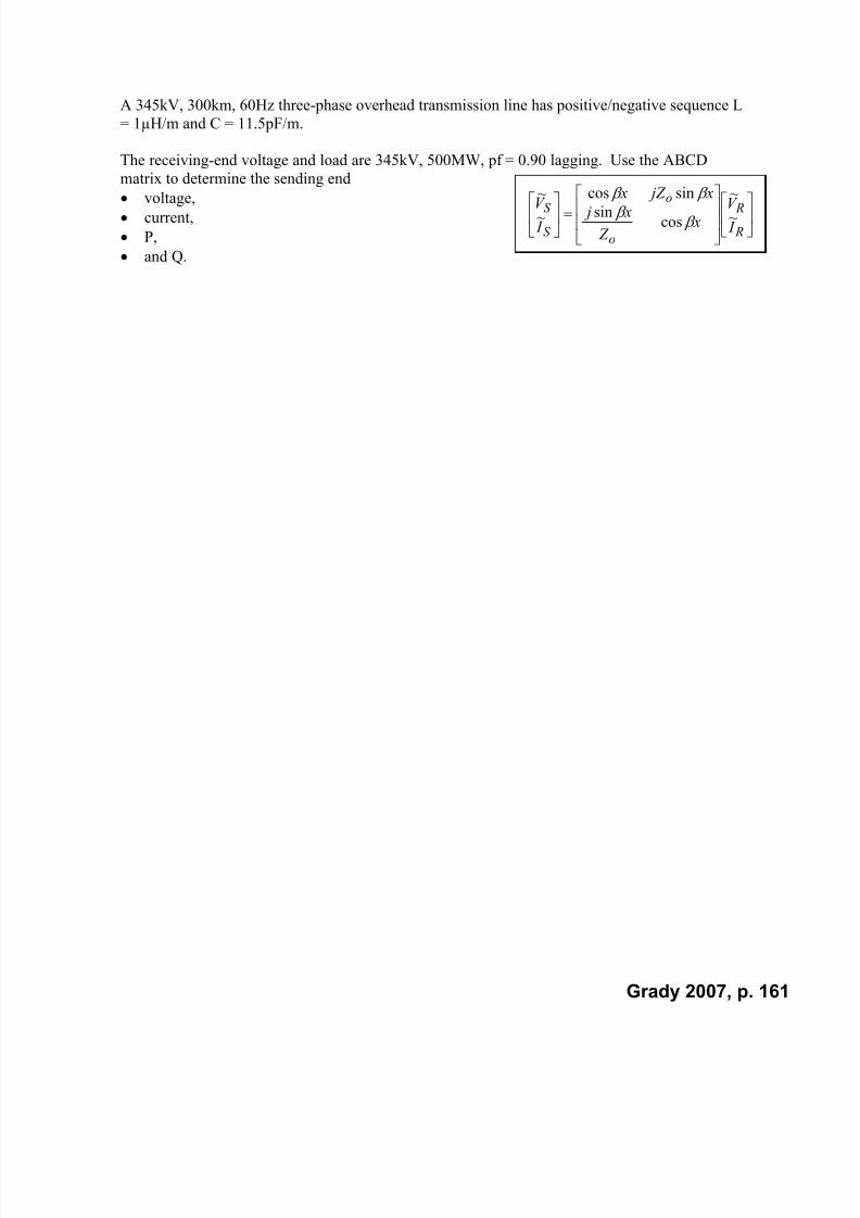
7/22/2019 Fundamentals Grady Notes June 2007 Print
http://slidepdf.com/reader/full/fundamentals-grady-notes-june-2007-print 161/388
A 345kV, 300km, 60Hz three-phase overhead transmission line has positive/negative sequence L
= 1µH/m and C = 11.5pF/m.
The receiving-end voltage and load are 345kV, 500MW, pf = 0.90 lagging. Use the ABCD
matrix to determine the sending end
voltage, current,
P,
and Q.
R
R
o
o
S
S
I V
x Z
x j
x jZ x
I V
~
~
cossin
sincos
~
~
Grady 2007, p. 161
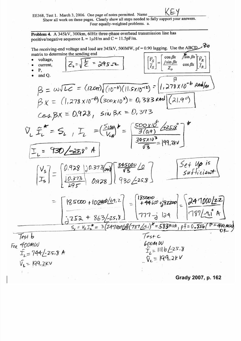
7/22/2019 Fundamentals Grady Notes June 2007 Print
http://slidepdf.com/reader/full/fundamentals-grady-notes-june-2007-print 162/388
Grady 2007, p. 162

7/22/2019 Fundamentals Grady Notes June 2007 Print
http://slidepdf.com/reader/full/fundamentals-grady-notes-june-2007-print 163/388
Grady 2007, p. 163
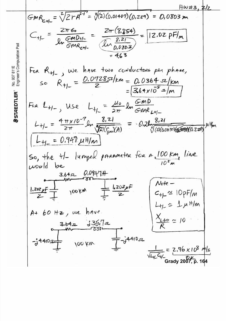
7/22/2019 Fundamentals Grady Notes June 2007 Print
http://slidepdf.com/reader/full/fundamentals-grady-notes-june-2007-print 164/388
Grady 2007, p. 164
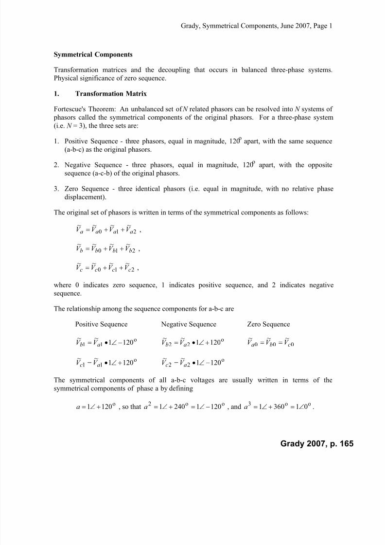
7/22/2019 Fundamentals Grady Notes June 2007 Print
http://slidepdf.com/reader/full/fundamentals-grady-notes-june-2007-print 165/388
Grady, Symmetrical Components, June 2007, Page 1
Symmetrical Components
Transformation matrices and the decoupling that occurs in balanced three-phase systems.
Physical significance of zero sequence.
1. Transformation Matrix
Fortescue's Theorem: An unbalanced set of N related phasors can be resolved into N systems of
phasors called the symmetrical components of the original phasors. For a three-phase system
(i.e. N = 3), the three sets are:
1. Positive Sequence - three phasors, equal in magnitude, 120o apart, with the same sequence
(a-b-c) as the original phasors.
2. Negative Sequence - three phasors, equal in magnitude, 120o apart, with the opposite
sequence (a-c-b) of the original phasors.
3. Zero Sequence - three identical phasors (i.e. equal in magnitude, with no relative phase
displacement).
The original set of phasors is written in terms of the symmetrical components as follows:
210~~~~aaaa V V V V ,
210~~~~bbbb V V V V ,
210
~~~~
cccc
V V V V ,
where 0 indicates zero sequence, 1 indicates positive sequence, and 2 indicates negative
sequence.
The relationship among the sequence components for a-b-c are
Positive Sequence Negative Sequence Zero Sequence
o11 1201
~~ ab V V o
22 1201~~
ab V V 000~~~cba V V V
o11 1201
~~
ac V V o
22 1201~~
ac V V
The symmetrical components of all a-b-c voltages are usually written in terms of the
symmetrical components of phase a by defining
o1201 a , so that oo2 12010421 a , and oo3 010631 a .
Grady 2007, p. 165
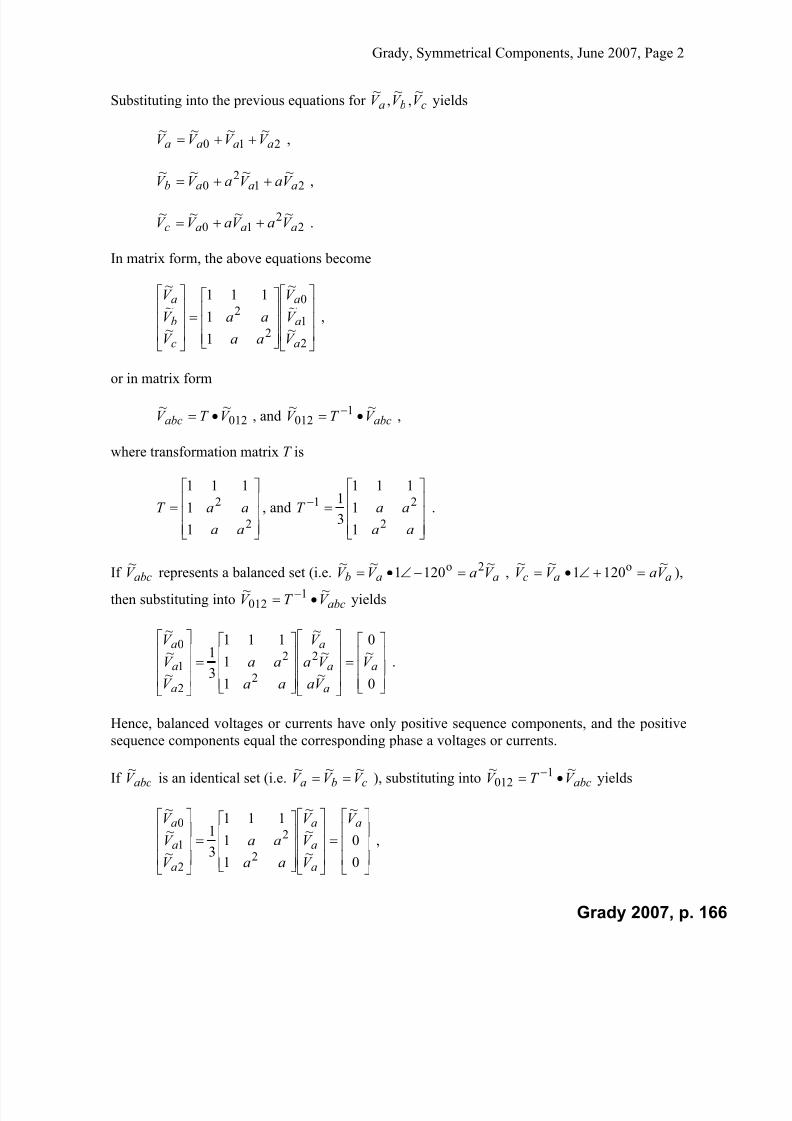
7/22/2019 Fundamentals Grady Notes June 2007 Print
http://slidepdf.com/reader/full/fundamentals-grady-notes-june-2007-print 166/388
Grady, Symmetrical Components, June 2007, Page 2
Substituting into the previous equations for cba V V V ~
,~
,~
yields
210~~~~aaaa V V V V ,
21
2
0
~~~~
aaab V aV aV V ,
22
10~~~~aaac V aV aV V .
In matrix form, the above equations become
2
1
0
2
2
~
~
~
1
1
111
~
~
~
a
a
a
c
b
a
V
V
V
aa
aa
V
V
V
,
or in matrix form
012~~V T V abc , and abcV T V
~~ 1012 ,
where transformation matrix T is
2
2
1
1
111
aa
aaT , and
aa
aaT 2
21
1
1
111
3
1 .
If abcV ~ represents a balanced set (i.e. aab V aV V ~1201~~ 2o , ~ ~ ~V V aV c a a 1 120o ),
then substituting into abcV T V ~~ 1
012 yields
0
~0
~
~
~
1
1
111
3
1
~
~
~
2
2
2
2
1
0
a
a
a
a
a
a
a
V
V a
V a
V
aa
aa
V
V
V
.
Hence, balanced voltages or currents have only positive sequence components, and the positive
sequence components equal the corresponding phase a voltages or currents.
If abcV ~
is an identical set (i.e. cba V V V ~~~
), substituting into abcV T V ~~ 1
012 yields
0
0
~
~
~
~
1
1
111
3
1
~
~
~
2
2
2
1
0 a
a
a
a
a
a
a V
V
V
V
aa
aa
V
V
V
,
Grady 2007, p. 166
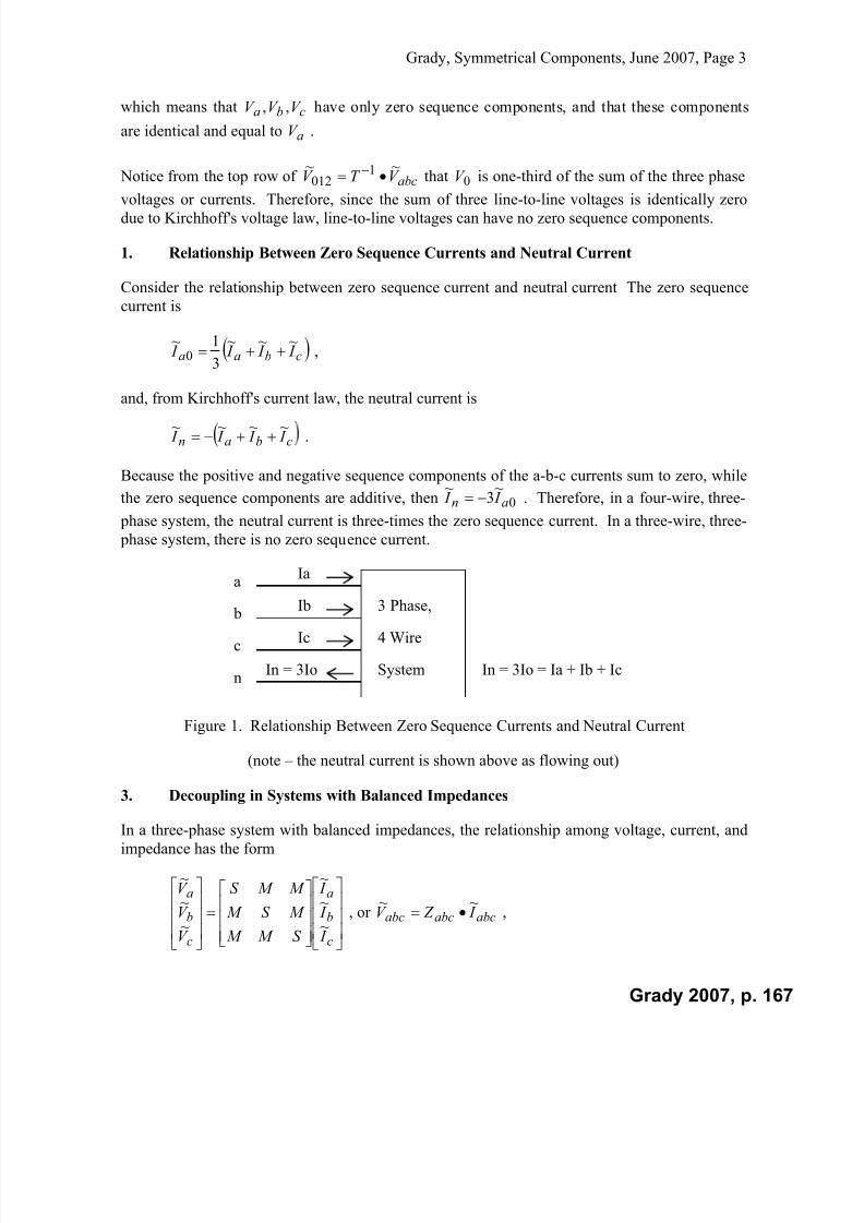
7/22/2019 Fundamentals Grady Notes June 2007 Print
http://slidepdf.com/reader/full/fundamentals-grady-notes-june-2007-print 167/388
Grady, Symmetrical Components, June 2007, Page 3
which means that cba V V V ,, have only zero sequence components, and that these components
are identical and equal to aV .
Notice from the top row of abcV T V ~~ 1
012 that 0V is one-third of the sum of the three phase
voltages or currents. Therefore, since the sum of three line-to-line voltages is identically zerodue to Kirchhoff's voltage law, line-to-line voltages can have no zero sequence components.
1. Relationship Between Zero Sequence Currents and Neutral Current
Consider the relationship between zero sequence current and neutral current The zero sequence
current is
cbaa I I I I ~~~
3
1~0 ,
and, from Kirchhoff's current law, the neutral current is
cban I I I I ~~~~
.
Because the positive and negative sequence components of the a-b-c currents sum to zero, while
the zero sequence components are additive, then 0~
3~
an I I . Therefore, in a four-wire, three-
phase system, the neutral current is three-times the zero sequence current. In a three-wire, three-
phase system, there is no zero sequence current.
Ia
Ib
Ic
In = 3Io
a
b
c
n
3 Phase,
4 Wire
In = 3Io = Ia + Ib + IcSystem
Figure 1. Relationship Between Zero Sequence Currents and Neutral Current
(note – the neutral current is shown above as flowing out)
3. Decoupling in Systems with Balanced Impedances
In a three-phase system with balanced impedances, the relationship among voltage, current, and
impedance has the form
c
b
a
c
b
a
I
I
I
S M M
M S M
M M S
V
V
V
~
~
~
~
~
~
, or abcabcabc I Z V ~~
,
Grady 2007, p. 167
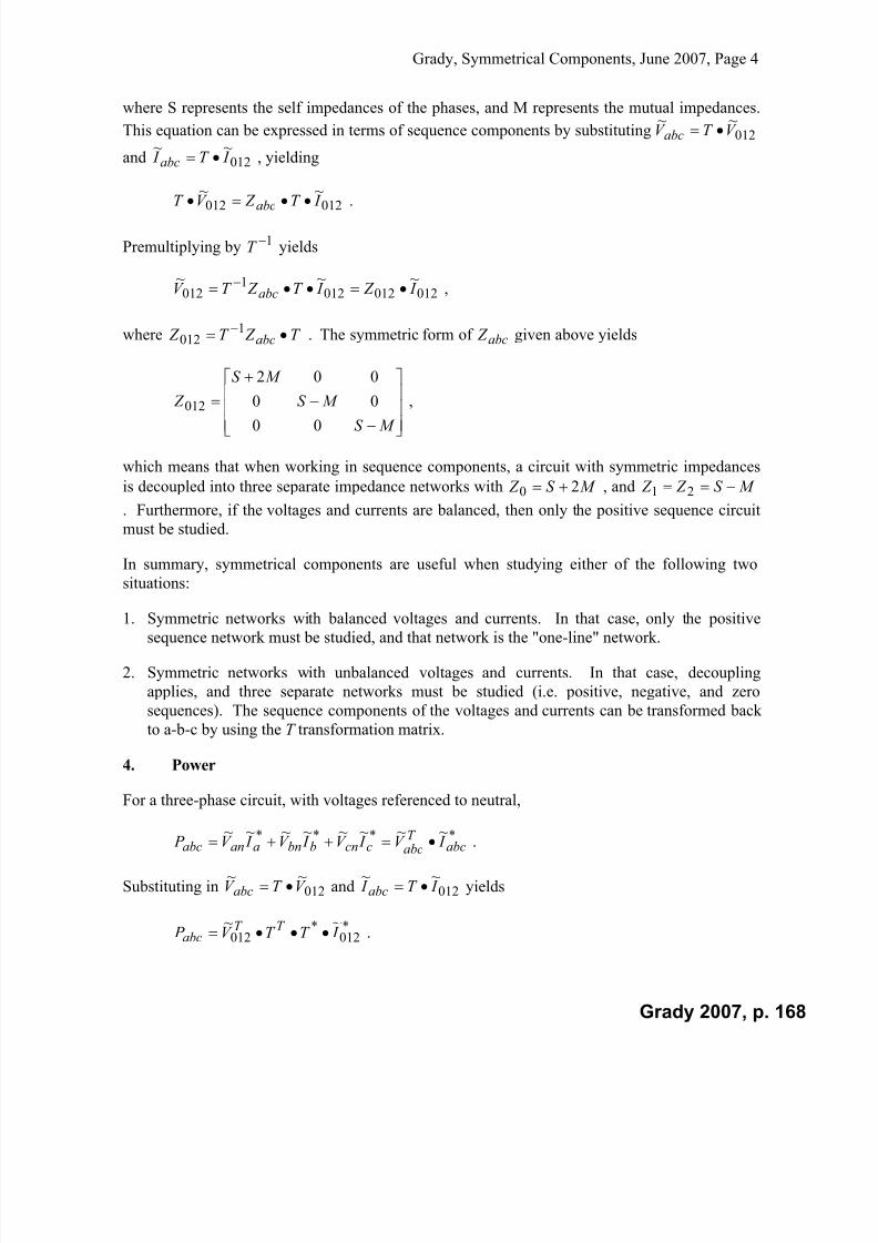
7/22/2019 Fundamentals Grady Notes June 2007 Print
http://slidepdf.com/reader/full/fundamentals-grady-notes-june-2007-print 168/388
Grady, Symmetrical Components, June 2007, Page 4
where S represents the self impedances of the phases, and M represents the mutual impedances.
This equation can be expressed in terms of sequence components by substituting 012~~V T V abc
and 012~~
I T I abc , yielding
012012
~~
I T Z V T abc .
Premultiplying by 1T yields
0120120121
012~~~ I Z I T Z T V abc ,
where T Z T Z abc 1012 . The symmetric form of abc Z given above yields
M S
M S
M S
Z
00
00
002
012 ,
which means that when working in sequence components, a circuit with symmetric impedances
is decoupled into three separate impedance networks with M S Z 20 , and M S Z Z 21
. Furthermore, if the voltages and currents are balanced, then only the positive sequence circuit
must be studied.
In summary, symmetrical components are useful when studying either of the following two
situations:
1. Symmetric networks with balanced voltages and currents. In that case, only the positivesequence network must be studied, and that network is the "one-line" network.
2. Symmetric networks with unbalanced voltages and currents. In that case, decoupling
applies, and three separate networks must be studied (i.e. positive, negative, and zero
sequences). The sequence components of the voltages and currents can be transformed back
to a-b-c by using the T transformation matrix.
4. Power
For a three-phase circuit, with voltages referenced to neutral,
**** ~~~~~~~~abc
T abcccnbbnaanabc I V I V I V I V P .
Substituting in 012~~V T V abc and 012
~~ I T I abc yields
*012
*012
~~ I T T V P
T T abc .
Grady 2007, p. 168
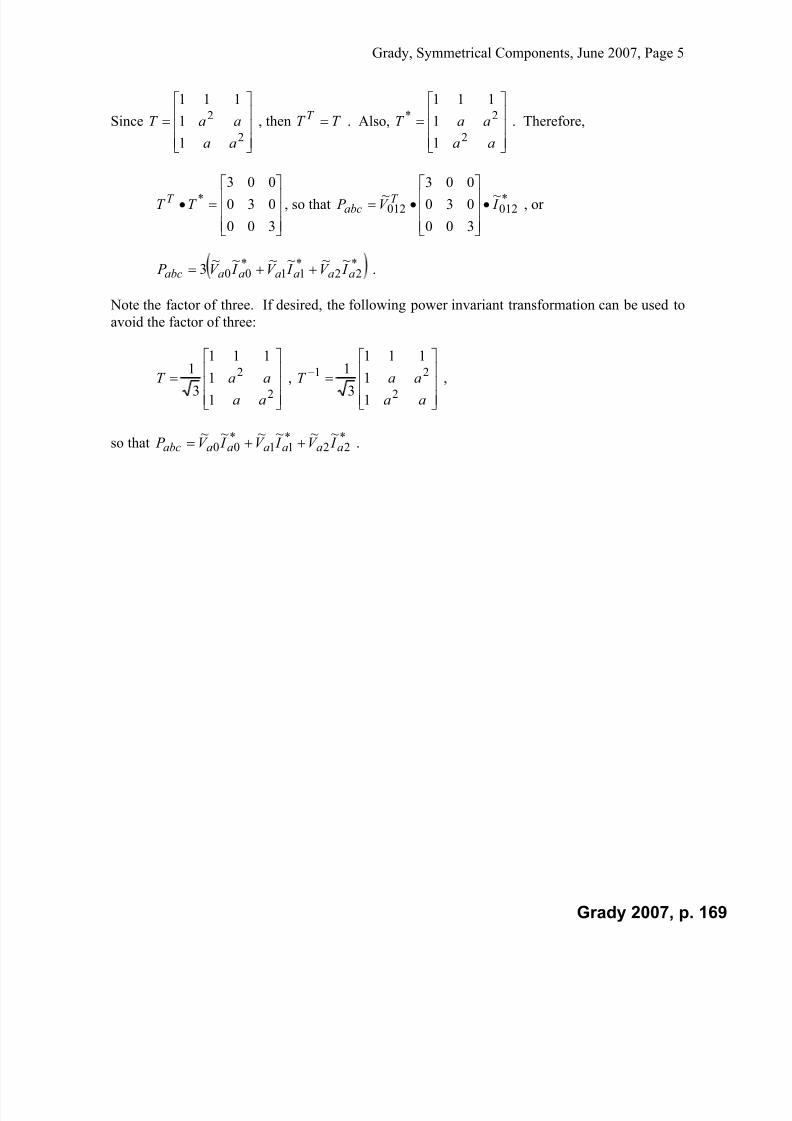
7/22/2019 Fundamentals Grady Notes June 2007 Print
http://slidepdf.com/reader/full/fundamentals-grady-notes-june-2007-print 169/388
Grady, Symmetrical Components, June 2007, Page 5
Since
2
2
1
1
111
aa
aaT , then T T T . Also,
aa
aaT 2
2*
1
1
111
. Therefore,
300
030003*T T T , so that *
012012~
300
030003~
I V P T abc
, or
*22
*11
*00
~~~~~~3 aaaaaaabc I V I V I V P .
Note the factor of three. If desired, the following power invariant transformation can be used to
avoid the factor of three:
2
2
1
1
111
31
aa
aaT ,
aa
aaT 2
21
1
1
111
31 ,
so that *22
*11
*00
~~~~~~aaaaaaabc I V I V I V P .
Grady 2007, p. 169
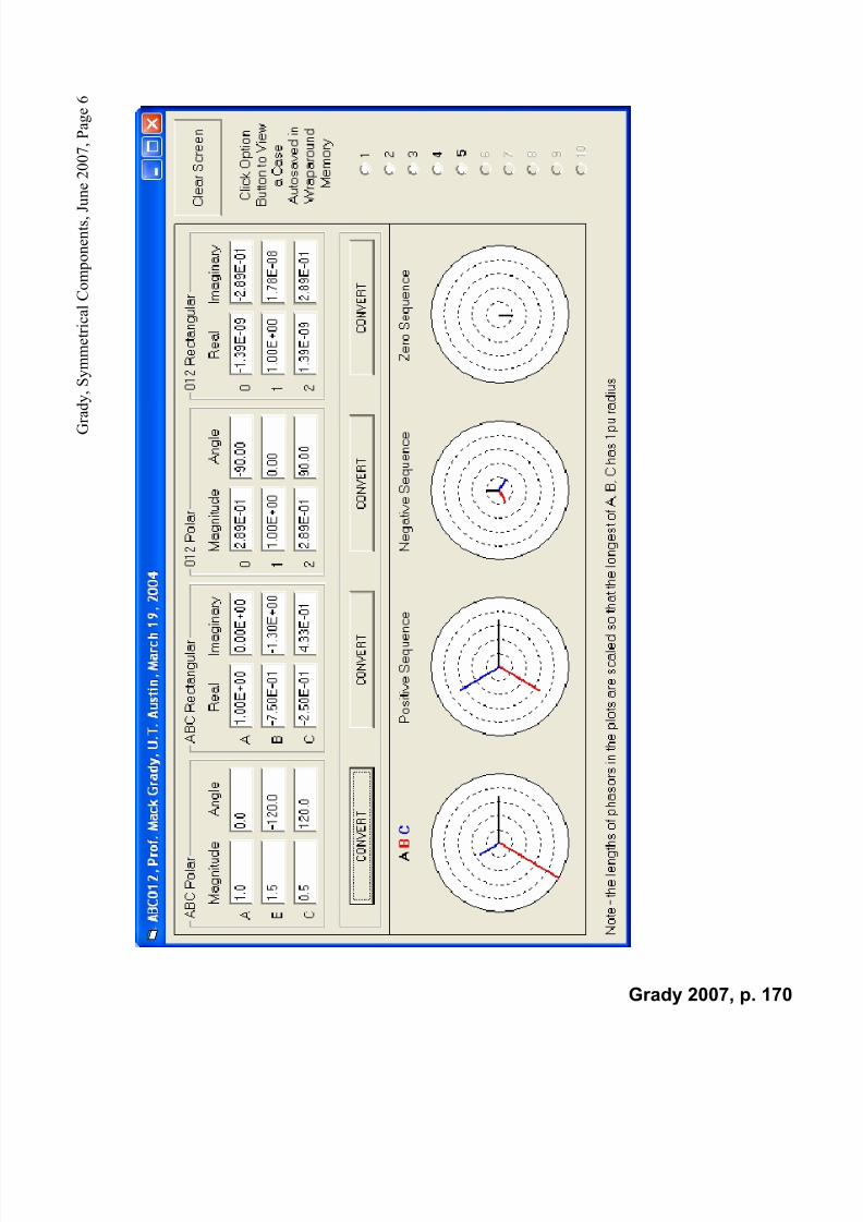
7/22/2019 Fundamentals Grady Notes June 2007 Print
http://slidepdf.com/reader/full/fundamentals-grady-notes-june-2007-print 170/388
G r a d y , S y m m e t r i c a l C o m p o n e n t s , J u
n e 2 0 0 7 , P a g e 6
Grady 2007, p. 170
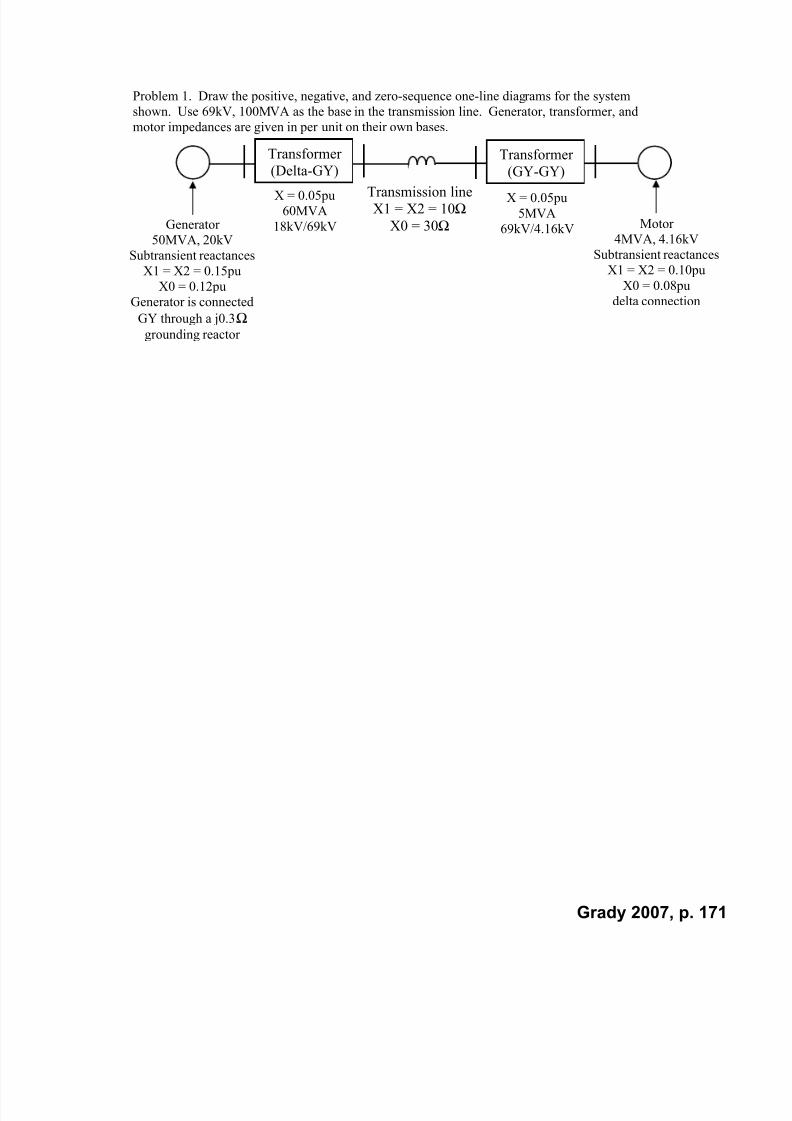
7/22/2019 Fundamentals Grady Notes June 2007 Print
http://slidepdf.com/reader/full/fundamentals-grady-notes-june-2007-print 171/388
Problem 1. Draw the positive, negative, and zero-sequence one-line diagrams for the system
shown. Use 69kV, 100MVA as the base in the transmission line. Generator, transformer, and
motor impedances are given in per unit on their own bases.
Generator
50MVA, 20kV
Subtransient reactances
X1 = X2 = 0.15pu
X0 = 0.12pu
Generator is connected
GY through a j0.3grounding reactor
X = 0.05pu
60MVA
18kV/69kV
Transformer
(Delta-GY)
X = 0.05pu
5MVA
69kV/4.16kV
Transformer
(GY-GY)
Motor
4MVA, 4.16kV
Subtransient reactances
X1 = X2 = 0.10pu
X0 = 0.08pu
delta connection
Transmission lineX1 = X2 = 10
X0 = 30
Grady 2007, p. 171

7/22/2019 Fundamentals Grady Notes June 2007 Print
http://slidepdf.com/reader/full/fundamentals-grady-notes-june-2007-print 172/388
Grady 2007, p. 172

7/22/2019 Fundamentals Grady Notes June 2007 Print
http://slidepdf.com/reader/full/fundamentals-grady-notes-june-2007-print 173/388
All impedances are given in per unit on system base. The generators have impedances
j0.10pu, and the transformers have impedances j0.08pu. The grounding reactor hasimpedance j0.05pu. Draw the zero-sequence network, showing impedance values. Identify
all nodes (i.e., P,Q,R,S,T,U,V,W, and ground).
Grady 2007, p. 173

7/22/2019 Fundamentals Grady Notes June 2007 Print
http://slidepdf.com/reader/full/fundamentals-grady-notes-june-2007-print 174/388
Grady 2007, p. 174

7/22/2019 Fundamentals Grady Notes June 2007 Print
http://slidepdf.com/reader/full/fundamentals-grady-notes-june-2007-print 175/388
Grady, System Matrices, June 2007, Page 1
Power System Matrices and Matrix Operations
Nodal equations using Kirchhoff's current law. Admittance matrix and building algorithm.
Gaussian elimination. Kron reduction. LU decomposition. Formation of impedance matrix by
inversion, Gaussian elimination, and direct building algorithm.
1. Admittance Matrix
Most power system networks are analyzed by first forming the admittance matrix. The
admittance matrix is based upon Kirchhoff's current law (KCL), and it is easily formed and very
sparse.
Consider the three-bus network shown in Figure that has five branch impedances and one current
source.
1 2 3
ZE
ZA
ZB
ZC
ZDI3
Figure 1. Three-Bus Network
Applying KCL at the three independent nodes yields the following equations for the bus voltages
(with respect to ground):
At bus 1, 0211
A E Z
V V
Z
V ,
At bus 2, 032122
C A B Z
V V
Z
V V
Z
V ,
At bus 3, 3233 I
Z
V V
Z
V
C D
.
Collecting terms and writing the equations in matrix form yields
Grady 2007, p. 175
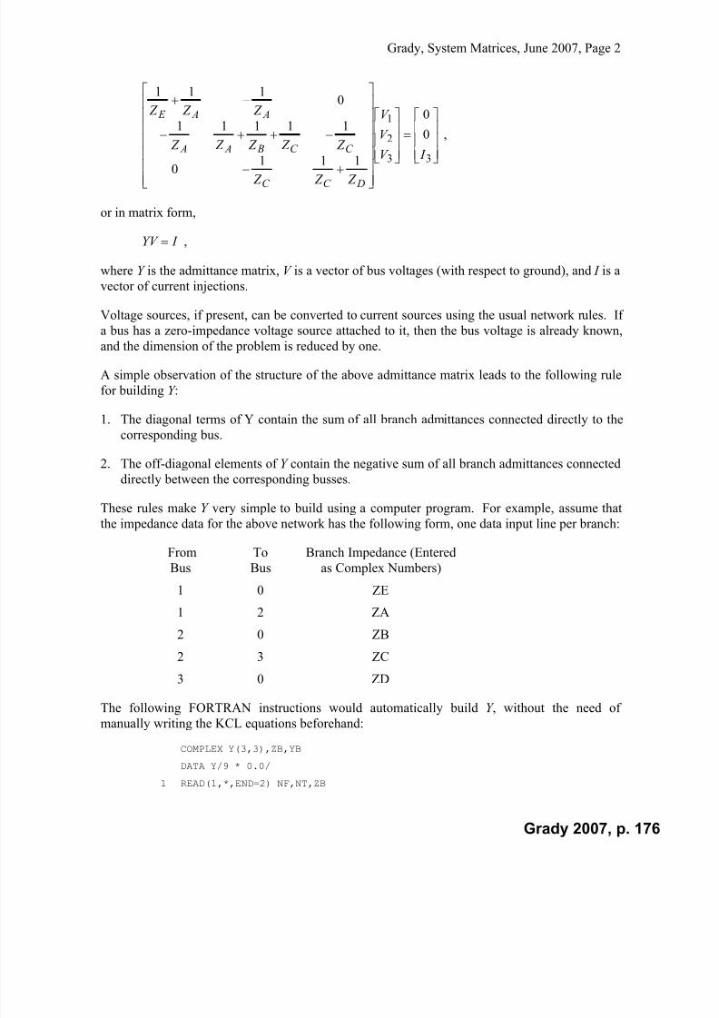
7/22/2019 Fundamentals Grady Notes June 2007 Print
http://slidepdf.com/reader/full/fundamentals-grady-notes-june-2007-print 176/388
Grady, System Matrices, June 2007, Page 2
33
2
1
0
0
1110
11111
0111
I V
V
V
Z Z Z
Z Z Z Z Z
Z Z Z
DC C
C C B A A
A A E
,
or in matrix form,
I YV ,
where Y is the admittance matrix, V is a vector of bus voltages (with respect to ground), and I is a
vector of current injections.
Voltage sources, if present, can be converted to current sources using the usual network rules. If
a bus has a zero-impedance voltage source attached to it, then the bus voltage is already known,
and the dimension of the problem is reduced by one.
A simple observation of the structure of the above admittance matrix leads to the following rule
for building Y :
1. The diagonal terms of Y contain the sum of all branch admittances connected directly to the
corresponding bus.
2. The off-diagonal elements of Y contain the negative sum of all branch admittances connected
directly between the corresponding busses.
These rules make Y very simple to build using a computer program. For example, assume thatthe impedance data for the above network has the following form, one data input line per branch:
From To Branch Impedance (Entered
Bus Bus as Complex Numbers)
1 0 ZE
1 2 ZA
2 0 ZB
2 3 ZC
3 0 ZD
The following FORTRAN instructions would automatically build Y , without the need of
manually writing the KCL equations beforehand:
COMPLEX Y(3,3),ZB,YB
DATA Y/9 * 0.0/
1 READ(1,*,END=2) NF,NT,ZB
Grady 2007, p. 176
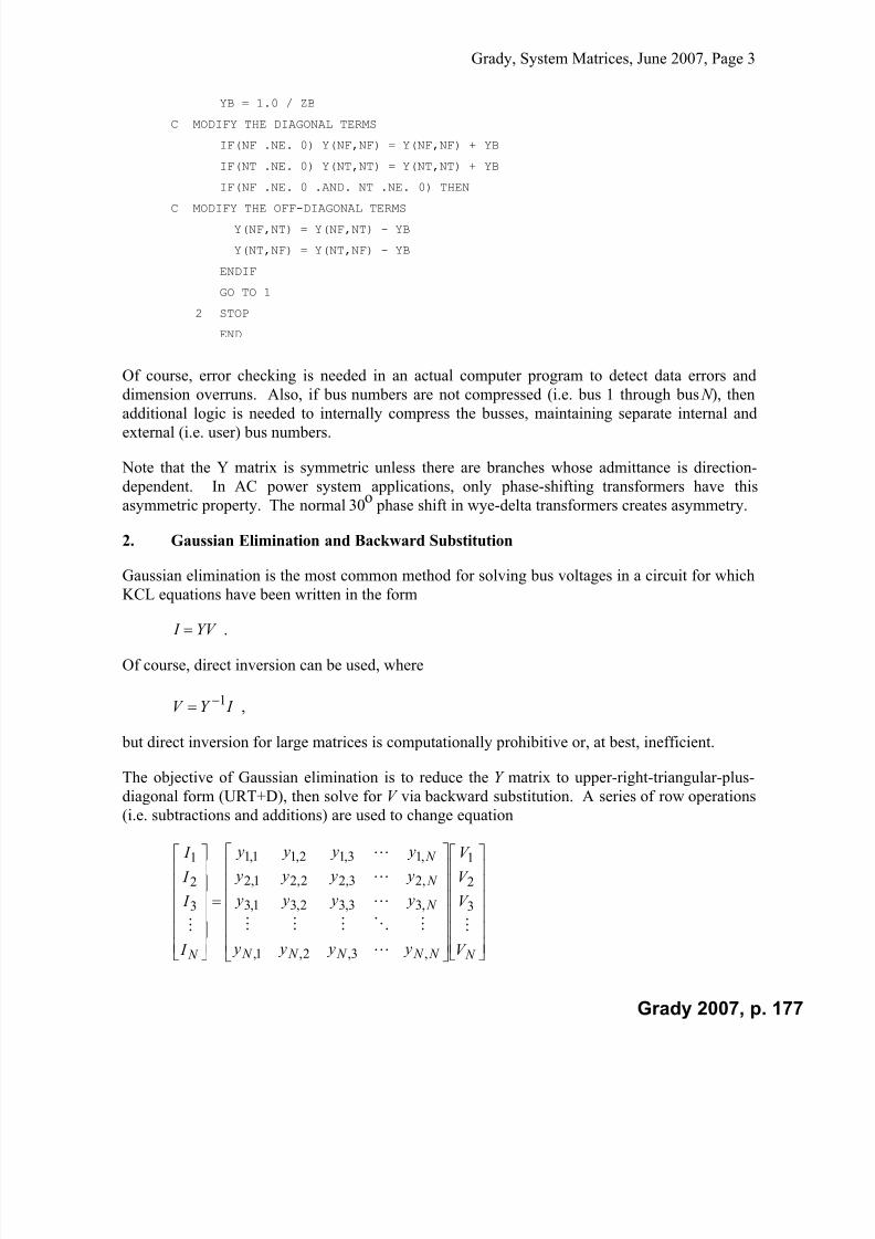
7/22/2019 Fundamentals Grady Notes June 2007 Print
http://slidepdf.com/reader/full/fundamentals-grady-notes-june-2007-print 177/388
Grady, System Matrices, June 2007, Page 3
YB = 1.0 / ZB
C MODIFY THE DIAGONAL TERMS
IF(NF .NE. 0) Y(NF,NF) = Y(NF,NF) + YB
IF(NT .NE. 0) Y(NT,NT) = Y(NT,NT) + YB
IF(NF .NE. 0 .AND. NT .NE. 0) THEN
C MODIFY THE OFF-DIAGONAL TERMS
Y(NF,NT) = Y(NF,NT) - YB
Y(NT,NF) = Y(NT,NF) - YB
ENDIF
GO TO 1
2 STOP
END
Of course, error checking is needed in an actual computer program to detect data errors and
dimension overruns. Also, if bus numbers are not compressed (i.e. bus 1 through bus N ), then
additional logic is needed to internally compress the busses, maintaining separate internal andexternal (i.e. user) bus numbers.
Note that the Y matrix is symmetric unless there are branches whose admittance is direction-
dependent. In AC power system applications, only phase-shifting transformers have this
asymmetric property. The normal 30o phase shift in wye-delta transformers creates asymmetry.
2. Gaussian Elimination and Backward Substitution
Gaussian elimination is the most common method for solving bus voltages in a circuit for which
KCL equations have been written in the form
YV I .
Of course, direct inversion can be used, where
I Y V 1 ,
but direct inversion for large matrices is computationally prohibitive or, at best, inefficient.
The objective of Gaussian elimination is to reduce the Y matrix to upper-right-triangular-plus-
diagonal form (URT+D), then solve for V via backward substitution. A series of row operations
(i.e. subtractions and additions) are used to change equation
N N N N N N
N
N
N
N V
V
V
V
y y y y
y y y y
y y y y
y y y y
I
I
I
I
3
2
1
,3,2,1,
,33,32,31,3
,23,22,21,2
,13,12,11,1
3
2
1
Grady 2007, p. 177
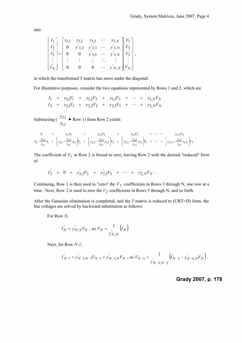
7/22/2019 Fundamentals Grady Notes June 2007 Print
http://slidepdf.com/reader/full/fundamentals-grady-notes-june-2007-print 178/388
Grady, System Matrices, June 2007, Page 4
into
N N N
N
N
N
N V
V
V
V
y
y y
y y y
y y y y
I
I
I
I
3
2
1
,'
,3'
3,3'
,2'
3,2'
2,2'
,13,12,11,1
'
'3
'2
1
000
00
0
,
in which the transformed Y matrix has zeros under the diagonal.
For illustrative purposes, consider the two equations represented by Rows 1 and 2, which are
N N
N N
V yV yV yV y I
V yV yV yV y I
,233,222,211,22
,133,122,111,11
.
Subtracting (1,1
1,2
y
y Row 1) from Row 2 yields
N N N
N N
V y y
y yV y
y
y yV y
y
y yV y
y
y y I
y
y I
V yV yV yV y I
,11,1
1,2,233,1
1,1
1,23,222,1
1,1
1,22,211,1
1,1
1,21,21
1,1
1,22
,133,122,111,11
.
The coefficient of 1V in Row 2 is forced to zero, leaving Row 2 with the desired "reduced" form
of
N N V yV yV y I ' ,23' 3,22' 2,2'2 0 .
Continuing, Row 1 is then used to "zero" the 1V coefficients in Rows 3 through N, one row at a
time. Next, Row 2 is used to zero the 2V coefficients in Rows 3 through N, and so forth.
After the Gaussian elimination is completed, and the Y matrix is reduced to (URT+D) form, the
bus voltages are solved by backward substitution as follows:
For Row N ,
N N N N V y I ' ,' , so '',
1 N
N N N I
yV .
Next, for Row N-1,
N N N N N N N V yV y I ',11
'1,1
'1 , so N N N N
N N
N V y I y
V ',1
'1'
1,1
11
.
Grady 2007, p. 178

7/22/2019 Fundamentals Grady Notes June 2007 Print
http://slidepdf.com/reader/full/fundamentals-grady-notes-june-2007-print 179/388
Grady, System Matrices, June 2007, Page 5
Continuing for Row j, where 2,,3,2 N N j ,
N N j j j j j j j j V yV yV y I ',1
'1,
',
' , so
N N j j j j j j j
j V yV y I y
V ',1
'1,
'
',
1
,
which, in general form, is described by
k k j
N
jk
j
j j
j V y I y
V ',
1
'
',
1 .
A simple FORTRAN computer program for solving V in an N-dimension problem using
Gaussian elimination and backward substitution is given below.
COMPLEX Y(N,N),V(N),I(N),YMM
C GAUSSIAN ELIMINATE Y AND I
NM1 = N - 1
C PIVOT ON ROW M, M = 1,2,3, ... ,N-1
DO 1 M = 1,NM1
MP1 = M + 1
YMM = 1.0 / Y(M,M)
C OPERATE ON THE ROWS BELOW THE PIVOT ROW
DO 1 J = MP1,N
C THE JTH ROW OF II(J) = I(J) - Y(J,M) *YMM * I(M)
C THE JTH ROW OF Y, BELOW AND TO THE RIGHT OF THE PIVOT
C DIAGONAL
DO 1 K = M,N
Y(J,K) = Y(J,K) - Y(J,M) * YMM * Y(M,K)
1 CONTINUE
C BACKWARD SUBSTITUTE TO SOLVE FOR V
V(N) = I(N) / Y(N,N)
DO 2 M = 1,NM1
J = N - M
C BACKWARD SUBSTITUTE TO SOLVE FOR V, FOR
C ROW J = N-1,N-2,N-3, ... ,1
V(J) = I(J)
JP1 = J + 1
DO 3 K = JP1,N
V(J) = V(J) - Y(J,K) * V(K)
Grady 2007, p. 179

7/22/2019 Fundamentals Grady Notes June 2007 Print
http://slidepdf.com/reader/full/fundamentals-grady-notes-june-2007-print 180/388
Grady, System Matrices, June 2007, Page 6
3 CONTINUE
V(J) = V(J) / Y(J,J)
2 CONTINUE
STOP
END
One disadvantage of Gaussian elimination is that if I changes, even though Y is fixed, the entire
problem must be re-solved since the elimination of Y determines the row operations that must be
repeated on I . Inversion and LU decomposition to not have this disadvantage.
3. Kron Reduction
Gaussian elimination can be made more computationally efficient by simply not performing
operations whose results are already known. For example, instead of arithmetically forcing
elements below the diagonal to zero, simply set them to zero at the appropriate times. Similarly,
instead of dividing all elements below and to the right of a diagonal element by the diagonal
element, divide only the elements in the diagonal row by the diagonal element, make the
diagonal element unity, and the same effect will be achieved. This technique, which is actually a
form of Gaussian elimination, is known as Kron reduction.
Kron reduction "pivots" on each diagonal element ',mm y , beginning with 1,1 y , and continuing
through 1,1 N N y . Starting with Row m = 1, and continuing through Row m = N - 1, the
algorithm for Kron reducing YV I is
1. Divide the elements in Row m, that are to the right of the diagonal, by the diagonal
element ',mm y . (Note - the elements to the left of the diagonal are already zero).
2. Replace element 'm I with
',
'
mm
m
y
I .
3. Replace diagonal element ',mm y with unity.
4. Modify the 'Y elements in rows greater than m and columns greater than m (i.e. below
and to the right of the diagonal element) using
',
',
',
', k mm jk jk j y y y y , for j > m, k > m.
5. Modify the ' I elements below the mth row according to
'',
''mm j j j I y I I , for j > m.
6. Zero the elements in Column m of 'Y that are below the diagonal element.
Grady 2007, p. 180
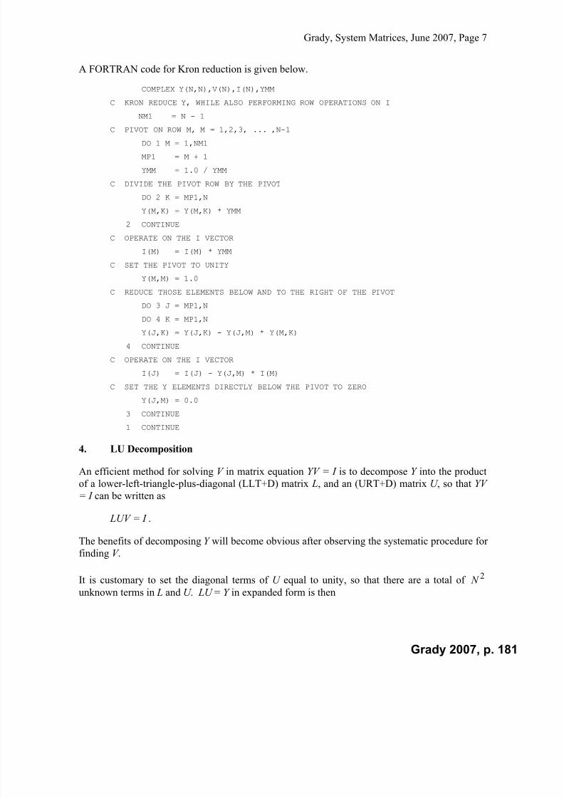
7/22/2019 Fundamentals Grady Notes June 2007 Print
http://slidepdf.com/reader/full/fundamentals-grady-notes-june-2007-print 181/388
Grady, System Matrices, June 2007, Page 7
A FORTRAN code for Kron reduction is given below.
COMPLEX Y(N,N),V(N),I(N),YMM
C KRON REDUCE Y, WHILE ALSO PERFORMING ROW OPERATIONS ON I
NM1 = N - 1
C PIVOT ON ROW M, M = 1,2,3, ... ,N-1DO 1 M = 1,NM1
MP1 = M + 1
YMM = 1.0 / YMM
C DIVIDE THE PIVOT ROW BY THE PIVOT
DO 2 K = MP1,N
Y(M,K) = Y(M,K) * YMM
2 CONTINUE
C OPERATE ON THE I VECTOR
I(M) = I(M) * YMM
C SET THE PIVOT TO UNITY
Y(M,M) = 1.0
C REDUCE THOSE ELEMENTS BELOW AND TO THE RIGHT OF THE PIVOT
DO 3 J = MP1,N
DO 4 K = MP1,N
Y(J,K) = Y(J,K) - Y(J,M) * Y(M,K)
4 CONTINUE
C OPERATE ON THE I VECTOR
I(J) = I(J) - Y(J,M) * I(M)
C SET THE Y ELEMENTS DIRECTLY BELOW THE PIVOT TO ZERO
Y(J,M) = 0.0
3 CONTINUE
1 CONTINUE
4. LU Decomposition
An efficient method for solving V in matrix equation YV = I is to decompose Y into the product
of a lower-left-triangle-plus-diagonal (LLT+D) matrix L, and an (URT+D) matrix U , so that YV
= I can be written as
LUV = I .
The benefits of decomposing Y will become obvious after observing the systematic procedure for
finding V .
It is customary to set the diagonal terms of U equal to unity, so that there are a total of 2 N
unknown terms in L and U . LU = Y in expanded form is then
Grady 2007, p. 181

7/22/2019 Fundamentals Grady Notes June 2007 Print
http://slidepdf.com/reader/full/fundamentals-grady-notes-june-2007-print 182/388
Grady, System Matrices, June 2007, Page 8
N N N N N
N
N
N
N
N
N
N N N N N y y y y
y y y y
y y y y
y y y y
u
uu
uuu
l l l l
l l l
l l
l
,3,2,1,
,33,32,31,3
,23,22,21,2
,13,12,11,1
,3
,23,2
,13,12,1
,3,2,1,
3,32,31,3
2,21,2
1,1
1000
100
10
1
0
00
000
.
Individual l and u terms are easily found by calculating them in the following order:
1. Starting from the top, work down Column 1 of L, finding 1,1l , then 1,2l , then 1,3l , ,
l N ,1 . For the special case of Column 1, these elements are 1,1, j j yl , j = 1,2,3, ,N .
2. Starting from the left, work across Row 1 of U , finding 2,1u , then 3,1u , then 4,1u , ,
N u ,1 . For the special case of Row 1, these elements are1,1
,1,1
l
yu
k k , k = 2,3,4, ,N .
3. Work down Column (k = 2) of L, finding 2,2l , then 2,3l , then 2,4l , , 2, N l , using
N k k k jul yl k m
k
mm jk jk j ,,2,1,,,
1
1
,,,
, Column N k k 2, .
4. Work across Row (k = 2) of U , finding 3,2u , then 4,2u , then 5,2u , , N u ,2 , using
N k k jl
ul y
uk k
k
m jmmk jk
jk ,,2+,1+=,,
1
1 ,,,
,
, Row )1(2, N k k .
5. Repeat Steps 3 and 4, first for Column k of L, then for Row k of U . Continue for all k =
3,4,5, ,( N 1) for L and U , then for k = N for L.
The procedure given above in Steps 1 - 5 is often referred to as Crout's method. Note that
elements of L and U never look "backward" for previously used elements of Y . Therefore, in
order to conserve computer memory, L and U elements can be stored as they are calculated in the
same locations at the corresponding Y elements. Thus, Crout's method is a memory-efficient "in
situ" procedure.
An intermediate column vector is needed to find V . The intermediate vector D is defined as
D = UV ,
so that
Grady 2007, p. 182

7/22/2019 Fundamentals Grady Notes June 2007 Print
http://slidepdf.com/reader/full/fundamentals-grady-notes-june-2007-print 183/388
Grady, System Matrices, June 2007, Page 9
N
N
N
N
N V
V
V
V
u
uu
uuu
d
d
d
d
3
2
1
,3
,23,2
,13,12,1
3
2
1
1000
100
10
1
.
Since LUV = I , then LD = I . Vector D is found using forward-substitution from
N N N N N N N I
I
I
I
d
d
d
d
l l l l
l l l
l l
l
3
2
1
3
2
1
,3,2,1,
3,32,31,3
2,21,2
1,1
0
00
000
,
which proceeds as follows:
From Row 1, 11,1
1111,11
, I l
d I d l ,
From Row 2, 11,222,2
2222,211,21
, d l I l
d I d l d l ,
From Row k ,
j jk
k
jk k k k k k k k k k
d l I l
d I d l d l d l ,
1
1,,22,11,
1, .
Now, since D = UV , or
N
N
N
N
N V
V
V
V
u
uu
uuu
d
d
d
d
3
2
1
,3
,23,2
,13,12,1
3
2
1
1000
100
10
1
,
where D and U are known, then V is found using backward substitution.
An important advantage of LU decomposition over Gaussian elimination or Kron reduction is
that the I vector is not modified during decomposition. Therefore, once Y has been decomposed
into L and U , I can be modified, and V recalculated, with minimal work, using the forward and
backward substitution steps shown above.
Grady 2007, p. 183

7/22/2019 Fundamentals Grady Notes June 2007 Print
http://slidepdf.com/reader/full/fundamentals-grady-notes-june-2007-print 184/388
Grady, System Matrices, June 2007, Page 10
A special form of L is helpful when Y is symmetric. In that case, let both L and U have unity
diagonal terms, and define a diagonal matrix D so that
Y = LDU ,
or
1000
100
10
1
000
000
000
000
1
0
01
001
0001
,3
,23,2
,13,12,1
,
3,3
2,2
1,1
3,2,1,
2,31,3
1,2
N
N
N
N N N N N
u
uu
uuu
d
d
d
d
l l l
l l
l
Y .
Since Y is symmetric, then T Y Y , and T T T T T T DLU L DU LDU LDU . Therefore,
an acceptable solution is to allow
T
U L . Incorporating this into the above equation yields
N N
N
N
N
N N N d
l d d
l d l d d
l d l d l d d
l l l
l l
l
Y
,
3,3,33,3
2,2,22,32,22,2
1,1,11,31,11,21,11,1
3,2,1,
2,31,3
1,2
000
00
0
1
0
01
001
0001
,
which can be solved by working from top-to-bottom, beginning with Column 1 of Y , as follows:
Working down Column 1 of Y ,
1,11,1 d y ,
1,11,21,21,11,21,2 /so, d yl d l y ,
1,11,1,1,11,1, /so, d yl d l y j j j j .
Working down Column 2 of Y ,
1,21,11,22,22,22,21,21,11,22,2so, l d l yd d l d l y ,
N jd l d l yl d l l d l y j j j j j j 2,/so, 2,21,21,11,2,2,2,22,1,21,11,2, .
Working down Column k of Y ,
Grady 2007, p. 184

7/22/2019 Fundamentals Grady Notes June 2007 Print
http://slidepdf.com/reader/full/fundamentals-grady-notes-june-2007-print 185/388
Grady, System Matrices, June 2007, Page 11
mk mm
k
m
mk k k k k k k mk mm
k
m
mk k k l d l yd d l d l y ,,
1
1,,,,,,
1
1,, so,
,
N jk d l d l yl l d l yk k mk mm
k
m m jk jk jmk mm
k
m m jk j
,/so,
,,,
1
1 ,,,,,
1
1 ,,
.
This simplification reduces memory and computation requirements for LU decomposition by
approximately one-half.
5. Bifactorization
Bifactorization recognizes the simple pattern that occurs when doing "in situ" LU
decomposition. Consider the first four rows and columns of a matrix that has been LU
decomposed according to Crout's method:
4,33,44,22,44,11,44,44,43,22,43,11,43,43,42,11,42,42,41,41,4
3,34,22,34,11,34,34,33,22,33,11,33,33,32,11,32,32,31,31,3
2,24,11,24,24,22,23,11,23,23,22,11,22,22,21,21,2
1,14,14,11,13,13,11,12,12,11,11,1
/
/////
ul ul ul yl ul ul yl ul yl yl
l ul ul yuul ul yl ul yl yl
l ul yul ul yuul yl yl l yul yul yu yl
.
The pattern developed is very similar to Kron reduction, and it can be expressed in the following
steps:
1. Beginning with Row 1, divide the elements to the right of the pivot element, and in the
pivot row, by 1,1l , so that
1,1
,1',1
y
y y
k k , for k = 2,3,4, , N .
2. Operate on the elements below and to the right of the pivot element using
',11,,
', k jk jk j y y y y , for j = 2,3,4, , N , k = 2,3,4, , N.
3. Continue for pivots m = 2,3,4, , ( N - 1) using
N mmk y
y y
mm
k mk m ,,2,1,
',
'
,', ,
followed by
N mmk N mm j y y y y k mm jk jk j ,,2,1;,,2,1,',
',
',
', ,
Grady 2007, p. 185

7/22/2019 Fundamentals Grady Notes June 2007 Print
http://slidepdf.com/reader/full/fundamentals-grady-notes-june-2007-print 186/388
Grady, System Matrices, June 2007, Page 12
for each pivot m.
When completed, matrix Y' has been replaced by matrices L and U as follows:
N N N N N l l l l
ul l l uul l
uuul
Y
,3,2,1,
5,33,32,31,3
5,23,22,21,2
5,13,12,11,1
'
,
and where the diagonal u elements are unity (i.e. 1,3,32,21,1 N N uuuu ).
The corresponding FORTRAN code for bifactorization is
COMPLEX Y(N,N),YMM
C DO FOR EACH PIVOT M = 1,2,3, ... ,N - 1
NM1 = N - 1
DO 1 M = 1,NM1
C FOR THE PIVOT ROW
MP1 = M + 1
YMM = 1.0 / Y(M,M)
DO 2 K = MP1,N
Y(M,K) = Y(M,K) * YMM
2 CONTINUE
C BELOW AND TO THE RIGHT OF THE PIVOT ELEMENT
DO 3 J = MP1,N
DO 3 K = MP1,N
Y(J,K) = Y(J,K) - Y(J,M) * Y(M,K)
3 CONTINUE
1 CONTINUE
STOP
END
6. Shipley-Coleman Inversion
For relatively small matrices, it is possible to obtain the inverse directly. The Shipley-Coleman
inversion method for inversion is popular because it is easily programmed. The algorithm is
1. For each pivot (i.e. diagonal term) m, m = 1,2,3, … , N , perform the following Steps 2 - 4.
2. Kron reduce all elements in Y , above and below, except those in Column m and Row musing
Grady 2007, p. 186

7/22/2019 Fundamentals Grady Notes June 2007 Print
http://slidepdf.com/reader/full/fundamentals-grady-notes-june-2007-print 187/388
Grady, System Matrices, June 2007, Page 13
mk N k m j N j y
y y y y
mm
k mm jk jk j ,,,3,2,1;,,,3,2,1,
,
',
','
,', .
3. Replace pivot element ',mm y with its negative inverse, i.e.
' ,
1
mm y
.
4. Multiply all elements in Row m and Column m, except the pivot, by ',mm y .
The result of this procedure is actually the negative inverse, so that when completed, all terms
must be negated. A FORTRAN code for Shipley-Coleman is shown below.
COMPLEX Y(N,N),YPIV
C DO FOR EACH PIVOT M = 1,2,3, ... ,N
DO 1 M = 1,N
YPIV = 1.0 / Y(M,M)C KRON REDUCE ALL ROWS AND COLUMNS, EXCEPT THE PIVOT ROW
C AND PIVOT COLUMN
DO 2 J = 1,N
IF(J .EQ. M) GO TO 2
DO 2 K = 1,N
IF(K. NE. M) Y(J,K) = Y(J,K) - Y(J,M) * Y(M,K) * YPIV
2 CONTINUE
C INVERT THE PIVOT ELEMENT AND NEGATE IT
YPIV = -YPIV
Y(M,M) = YPIV
C WORK ACROSS THE PIVOT ROW AND DOWN THE PIVOT COLUMN,
C MULTIPLYING BY THE NEW PIVOT VALUE
DO 3 K = 1,N
IF(K .EQ. M) GO TO 3
Y(M,K) = Y(M,K) * YPIV
Y(K,M) = Y(K,M) * YPIV
3 CONTINUE
1 CONTINUE
C NEGATE THE RESULTS
DO 4 J = 1,N
DO 4 K = 1,N
Y(J,K) = -Y(J,K)
4 CONTINUE
STOP
END
Grady 2007, p. 187

7/22/2019 Fundamentals Grady Notes June 2007 Print
http://slidepdf.com/reader/full/fundamentals-grady-notes-june-2007-print 188/388
Grady, System Matrices, June 2007, Page 14
The order of the number of calculations for Shipley-Coleman is 3 N .
7. Impedance Matrix
The impedance matrix is the inverse of the admittance matrix, or
1 Y Z ,
so that
ZI V .
The reference bus both Y and Z is ground. Although the impedance matrix can be found via
inversion, complete inversion is not common for matrices with more than a few hundred rows
and columns because of the matrix storage requirements. In those instances, Z elements are
usually found via Gaussian elimination, Kron reduction, or, less commonly, by a direct building
algorithm. If only a few of the Z elements are needed, then Gaussian elimination or Kronreduction are best. Both methods are described in following sections.
8. Physical Significance of Admittance and Impedance Matrices
The physical significance of the admittance and impedance matrices can be seen by examining
the basic matrix equations YV I and ZI I Y V 1 . Expanding the jth row of YV I yields
N
k
k k j j V y I
1, . Therefore,
k m N mmV k
jk j
V I y
,,,2,1,0
,
,
where, as shown in Figure 2, all busses except k are grounded, k V is a voltage source attached to
bus k , and j I is the resulting current injection at (i.e. flowing into) bus j. Since all busses that
neighbor bus k are grounded, the currents induced by k V will not get past these neighbors, and
the only non-zero injection currents j I will occur at the neighboring busses. In a large power
system, most busses do not neighbor any arbitrary bus k . Therefore, Y consists mainly of zeros
(i.e. is sparse) in most power systems.
Grady 2007, p. 188

7/22/2019 Fundamentals Grady Notes June 2007 Print
http://slidepdf.com/reader/full/fundamentals-grady-notes-june-2007-print 189/388
Grady, System Matrices, June 2007, Page 15
+
-
Vk
Bus jApplied Voltage
Power System
Ij
All Other Busses
Grounded
at Bus k
Induced Current at
A
Figure 2. Measurement of Admittance Matrix Term k j y ,
Concerning Z , the kth row of ZI I Y V 1 yields
N
j
j jk k I z V
1
, . Hence,
k m N mm I k
jk j
I
V z
,,,2,1,0
,
,
where, as shown in Figure 3, I k is a current source attached to bus k , V j is the resulting voltage at
bus j, and all busses except k are open-circuited. Unless the network is disjoint, then current
injection at one bus, when all other busses open-circuited, will raise the potential everywhere in
the network. For that reason, Z tends to be full.
Power System
All Other Busses
Open Circuited
Applied Current atInduced Voltage
+
-
V
Bus k at Bus j
Ik
Vj
Figure 3. Measurement of Impedance Matrix Term k j z ,
9. Formation of the Impedance Matrix via Gaussian Elimination, Kron Reduction,and LU Decomposition
Gaussian Elimination
An efficient method of fully or partially inverting a matrix is to formulate the problem using
Gaussian elimination. For example, given
Grady 2007, p. 189

7/22/2019 Fundamentals Grady Notes June 2007 Print
http://slidepdf.com/reader/full/fundamentals-grady-notes-june-2007-print 190/388
Grady, System Matrices, June 2007, Page 16
I YZ ,
where Y is a matrix of numbers, Z is a matrix of unknowns, and I is the identity matrix, the
objective is to Gaussian eliminate Y , while performing the same row operations on I , to obtain
the form
I Z Y ,
where Y' is in (URT+D) form. Then, individual columns of Z can then be solved using backward
substitution, one at a time. This procedure is also known as the augmentation method, and it is
illustrated as follows:
Y is first Gaussian eliminated, as shown in a previous section, while at the same time performing
identical row operations on I . Afterward, the form of I Z Y is
N N N N N
N N
N
N N
N N
N
z z z z
z z z z
z z z z
z z z z
y
y y y y y
y y y y
,3,2,1,
,33,32,31,3,23,22,21,2
,13,12,11,1
,'
,3'
3,3' ,2
'
3,2
'
2,2
',13,12,11,1
000
000
'
,
'
3,
'
2,
'
1,
'3,3
'2,3
'1,3
'2,2
'1,2
0
00
0001
N N N N N I I I I
I I I
I I
where Rows 1 of Y' and I' are the same as in Y and I . The above equation can be written in
abbreviated column form as
''3
'2
'1321
,'
,3'
3,3'
,2'
3,2'
2,2'
,13,12,11,1
000
00
0
N N
N N
N
N
N
I I I I Z Z Z Z
y
y y
y y y
y y y y
,
where the individual column vectors Z i and I i have dimension N x 1. The above equation can be
solved as N separate subproblems, where each subproblem computes a column of Z . For
example, the kth column of Z can be computed by applying backward substitution to
Grady 2007, p. 190

7/22/2019 Fundamentals Grady Notes June 2007 Print
http://slidepdf.com/reader/full/fundamentals-grady-notes-june-2007-print 191/388
Grady, System Matrices, June 2007, Page 17
',
',3
',2
',1
,
,3
,2
,1
,'
,3'
3,3'
,2'
3,2'
2,2'
,13,12,11,1
000
00
0
k N
k
k
k
k N
k
k
k
N N
N
N
N
I
I
I
I
Z
Z
Z
Z
y
y y
y y y
y y y y
.
Each column of Z is solved independently from the others.
Kron Reduction
If Kron reduction, the problem is essentially the same, except that Row 1 of the above equation
is divided by '1,1 y , yielding
',
',3
',2
'
,1
,
,3
,2,1
,'
,3'
3,3'
,2'
3,2'
2,2' ,13,12,11,1
000
00
0
k N
k
k k
k N
k
k k
N N
N
N N
I
I
I
I
Z
Z
Z
Z
y
y y
y y y
y y y y
.
Because backward substitution can stop when the last desired z element is computed, the process
is most efficient if the busses are ordered so that the highest bus numbers (i.e. N , N-1, N-2, etc.)
correspond to the desired z elements. Busses can be ordered accordingly when forming Y to take
advantage of this efficiency.
LU Decomposition
Concerning LU decomposition, once the Y matrix has been decomposed into L and U , then we
have
I LUZ YZ ,
where I is the identity matrix. Expanding the above equation as I UZ L yields
N N N N N
N
N
N
N N N N N uz uz uz uz
uz uz uz uz
uz uz uz uz
uz uz uz uz
l l l l
l l l
l l
l
,3,2,1,
,33,32,31,3
,23,22,21,2
,13,12,11,1
,3,2,1,
3,33,21,3
2,21,2
1,1
0
00
000
.
Grady 2007, p. 191

7/22/2019 Fundamentals Grady Notes June 2007 Print
http://slidepdf.com/reader/full/fundamentals-grady-notes-june-2007-print 192/388
Grady, System Matrices, June 2007, Page 18
1000
0100
0010
0001
The special structure of the above equation shows that, in general, UZ must be (LLT+D) in form.
UZ can be found by using forward substitution on the above equation, and then Z can be found,
one column at a time, by using backward substitution on Z U UZ , which in expanded form
is
N N N N N
N
N
N
N
N
N
z z z z
z z z z
z z z z
z z z z
u
uu
uuu
,3,2,1,
,33,32,31,3
,23,22,21,2
,13,12,11,1
,3
,23,2
,13,12,1
1000
100
10
1
N N N N N uz uz uz uz
uz uz uz
uz uz
uz
,3,2,1,
3,32,31,3
2,21,2
1,1
0
00
000
.
10. Direct Impedance Matrix Building and Modification Algorithm
The impedance matrix can be built directly without need of the admittance matrix, if the physical
properties of Z are exploited. Furthermore, once Z has been built, no matter which method was
used, it can be easily modified when network changes occur. This after-the-fact modification
capability is the most important feature of the direct impedance matrix building and modification
algorithm.
The four cases to be considered in the algorithm are
Case 1. Add a branch impedance between a new bus and the reference bus.
Case 2. Add a branch impedance between a new bus and an existing non-reference bus.
Case 3. Add a branch impedance between an existing bus and the reference bus.
Case 4. Add a branch impedance between two existing non-reference busses.
Direct formation of an impedance matrix, plus all network modifications, can be achieved
through these four cases. Each of the four is now considered separately.
Grady 2007, p. 192

7/22/2019 Fundamentals Grady Notes June 2007 Print
http://slidepdf.com/reader/full/fundamentals-grady-notes-june-2007-print 193/388
Grady, System Matrices, June 2007, Page 19
Case 1, Add a Branch Impedance Between a New Bus and the Reference Bus
Case 1 is applicable in two situations. First, it is the starting point when building a new
impedance matrix. Second, it provides (as does Case 2) a method for adding new busses to an
existing impedance matrix.
Both situations applicable to Case 1 are shown in Figure 4. The starting-point situation is on the
left, and the new-bus situation is on the right.
Power System N Busses
Zadd
Bus 1
ReferenceBus
Zadd
Bus (N+1)
Situation 1 Situation 2
ReferenceBus
Figure 4. Case 1, Add a Branch Impedance Between a New Bus and the Reference Bus
The impedance matrices for the two situations are
Situation 1 Zadd Z 1,1 ,
Situation 2:
111
1
,1,1
000
0
0
0
x xN
Nx
NxN N N N N
Zadd
Z Z
.
The effect of situation 2 is simply to augment the existing N N Z , by a column of zeros, a row of
zeros, and a new diagonal element Zadd . New bus ( N+1) is isolated from the rest of the system.
Case 2, Add a Branch Impedance Between a New Bus and an Existing Non-Reference Bus
Consider Case 2, shown in Figure 5, where a branch impedance Zadd is added from existing
non-reference bus j to new bus ( N+1). Before the addition, the power system has N busses, plusa reference bus (which is normally ground), and an impedance matrix N N Z , .
Grady 2007, p. 193
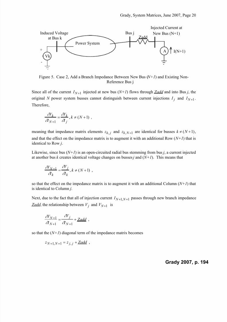
7/22/2019 Fundamentals Grady Notes June 2007 Print
http://slidepdf.com/reader/full/fundamentals-grady-notes-june-2007-print 194/388
Grady, System Matrices, June 2007, Page 20
+
-
Vk
Bus j
Power System
at Bus k
A
Induced Voltage
Injected Current at
I(N+1)
Zadd New Bus (N+1)
Figure 5. Case 2, Add a Branch Impedance Between New Bus ( N+1) and Existing Non-
Reference Bus j
Since all of the current 1 N I injected at new bus ( N+1) flows through Zadd and into Bus j, the
original N power system busses cannot distinguish between current injections j I and 1 N I .
Therefore,
)1(,1
N k I
V
I
V
j
k
N
k
,
meaning that impedance matrix elements jk z , and 1, N k z are identical for busses k N ( )1 ,
and that the effect on the impedance matrix is to augment it with an additional Row ( N+1) that is
identical to Row j.
Likewise, since bus ( N+1) is an open-circuited radial bus stemming from bus j, a current injected
at another bus k creates identical voltage changes on busses j and ( N+1). This means that
)1(,1 N k I
V
I
V
k
j
k
N
,
so that the effect on the impedance matrix is to augment it with an additional Column ( N+1) that
is identical to Column j.
Next, due to the fact that all of injection current 1,1 N N I passes through new branch impedance
Zadd , the relationship between jV and 1 N V is
Zadd I
V
I
V
N
j
N
N
11
1
,
so that the ( N+1) diagonal term of the impedance matrix becomes
Zadd z z j j N N ,1,1 ,
Grady 2007, p. 194

7/22/2019 Fundamentals Grady Notes June 2007 Print
http://slidepdf.com/reader/full/fundamentals-grady-notes-june-2007-print 195/388
Grady, System Matrices, June 2007, Page 21
where j j z , is the jth diagonal term of NxN Z .
Summarizing, the total effect of Case 2 is to increase the dimension of the impedance matrix by
one row and column according to
11,1,
1,,1,1 of Row
of Column
x j j xN N N
Nx N N NxN N N N N Zadd z Z j
Z j Z Z .
Case 3, Add a Branch Impedance Between an Existing Bus and the Reference Bus
Now, consider Case 3, where a new impedance-to-reference tie Zadd is added to existing Bus j.
The case is handled as a two-step extension of Case 2, as shown in Figure 4.6. First, extend
Zadd from Bus j to fictitious Bus ( N+1), as was done in Case 2. Then, tie fictitious Bus ( N+1)
to the reference bus, and reduce the size of the augmented impedance matrix back to ( N x N ).
Bus j
Power System
New Bus (N+1)
Step 1 Step 2
Bus j
Power System
Zadd
Zadd
Figure 6. Case 3. Two-Step Procedure for Adding Branch Impedance Zadd from Existing Bus jto the Reference Bus
Step 1 creates the augmented 1,1 N N Z matrix shown in Case 2. The form of equation
N N N N I Z V 1,11 is
REF
Nx
x j j xN N N
Nx N N NxN N N
REF
Nx
I
I
Zadd z Z j
Z j Z
V
V 1
11,1,
1,,1
of Row
of Column
0 ,
where REF j j REF I Zadd z V and,, , are scalars. Defining the row and column vectors as j R
and jC , respectively, yields
REF
Nx
x j j xN j
Nx NxN N N
REF
Nx
I
I
Zadd z R
Z
V
V 1
11,1
1 j,1C
0 .
At this point, scalar REF I can be eliminated by expanding the bottom row to obtain
Grady 2007, p. 195
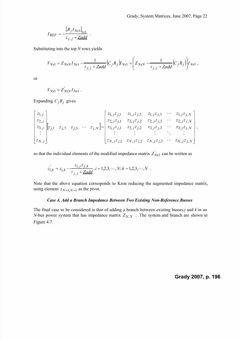
7/22/2019 Fundamentals Grady Notes June 2007 Print
http://slidepdf.com/reader/full/fundamentals-grady-notes-june-2007-print 196/388
Grady, System Matrices, June 2007, Page 22
Zadd z
I R I
j j
x Nx j
REF
,
111 .
Substituting into the top N rows yields
1,
1,
1111
Nx j j j j
NxN Nx j j j j
Nx NxN Nx I RC Zadd z
Z I RC Zadd z
I Z V
,
or
1'
1 Nx NxN Nx I Z V .
Expanding j j RC gives
N j j N j j N j j N j j N
N j j j j j j j j
N j j j j j j j j
N j j j j j j j j
N j j j j
j N
j
j
j
z z z z z z z z
z z z z z z z z
z z z z z z z z z z z z z z z z
z z z z
z
z
z z
,,3,,2,,1,,
,,33,,32,,31,,3
,,23,,22,,21,,2
,,13,,12,,11,,1
,3,2,1,
,
,3
,2
,1
,
so that the individual elements of the modified impedance matrix '1 Nx Z can be written as
N k N i Zadd z
z z
z z j j
k j ji
k ik i ,,3,2,1;,,3,2,1,,
,,
,
'
,
.
Note that the above equation corresponds to Kron reducing the augmented impedance matrix,
using element 1,1 N N z as the pivot.
Case 4, Add a Branch Impedance Between Two Existing Non-Reference Busses
The final case to be considered is that of adding a branch between existing busses j and k in an
N -bus power system that has impedance matrix N N Z , . The system and branch are shown in
Figure 4.7.
Grady 2007, p. 196

7/22/2019 Fundamentals Grady Notes June 2007 Print
http://slidepdf.com/reader/full/fundamentals-grady-notes-june-2007-print 197/388
Grady, System Matrices, June 2007, Page 23
Power System
Zadd
Reference Bus
Bus j
Ij
Ib
Ij - Ib
Bus k
Ik Ik + Ib
Ib
with N Busses
Figure 7. Case 4, Add Branch Impedance Zadd between Existing Busses j and k
As seen in the figure, the actual current injected into the system via Bus j is b j I I , and the
actual injection via Bus k is bk I I , where
Zadd
V V I
k jb
, or bk j I Zadd V V .
The effect of the branch addition on the voltage at arbitrary bus m can be found by substituting
the true injection currents at busses j and k into I Z V N N , , yielding
b j jmmmmm I I z I z I z I z V ,33,22,11,
N N mbk k m I z I I z ,, ,
or
k k m j jmmmmm I z I z I z I z I z V ,,33,22,11,
bk m jm N N m I z z I z ,,, .
For busses j and k specifically,
b j jk k k k
b j j j j j j
k
j
I I z I z I z I z
I I z I z I z I z
V
V
,33,22,11,
,33,22,11,
N N k bk k k
N N jbk k j
I z I I z
I z I I z
,,
,,
.
Then, k j V V gives
Grady 2007, p. 197

7/22/2019 Fundamentals Grady Notes June 2007 Print
http://slidepdf.com/reader/full/fundamentals-grady-notes-june-2007-print 198/388
Grady, System Matrices, June 2007, Page 24
,,33,3,22,2,11,1, b j jk j jk jk jk jk j I I z z I z z I z z I z z V V
N N k N jbk k k k j I z z I I z z ,,,, .
Substituting in bk j
I Zadd V V and combining terms then yields
0 ,,33,3,22,2,11,1, j jk j jk jk jk j I z z I z z I z z I z z
b jk k jk k j j N N k N jk k k k j I Zadd z z z z I z z I z z ,,,,,,,, .
All of the above effects can be included as an additional row and column in equation
I Z V N N , as follows:
1,,,,1,,
1,,,
1
1
f R f Row
f Colf Col
0 Nx jk k jk k j j xN N N N N
Nx N N N N NxN N N
Nx
Nx N
Zadd z z z z Z ok ow Z o j
Z ok Z o j Z V .
11
1
xb
Nx N
I
I .
As was done in Case 3, the effect of the augmented row and column of the above equation can be
incorporated into a modified impedance matrix by using Kron reduction, where element z N N 1 1,
is the pivot, yielding
Zadd z z z z
z z z z z z
jk k jk k j j
mk m jk i ji
mimi
,,,,
,,,,
,
'
, .
Application Notes
Once an impedance matrix is built, no matter which method is used, the modification algorithm
can very easily adjust Z for network changes. For example, a branch outage can be effectively
achieved by placing an impedance, of the same but negative value, in parallel with the actual
impedance, so that the impedance of the parallel combination is infinite.
11. Example Code YZBUILD for Building Admittance Matrix and Impedance Matrixc
c program yzbuild. 10/10/04.c implicit none
complex ybus,yline,ycap,ctap,yii,ykk,yik,ykicomplex lmat,umat,unity,czero,ytest,ysave,diff,uz,1 uzelem,zbus,elem,alphainteger nb,nbus,nfrom,nto,j,k,ipiv,jdum,kdum,jm1,kp1,linteger nlu,ipiv1,nm1,ny,nbext,nbint,iout,mxext,mxintinteger jp1,ipp1,ngy,ngureal eps4,eps6,eps9,pi,dr,qshunt,r,x,charge,fill,ymag,umag
Grady 2007, p. 198
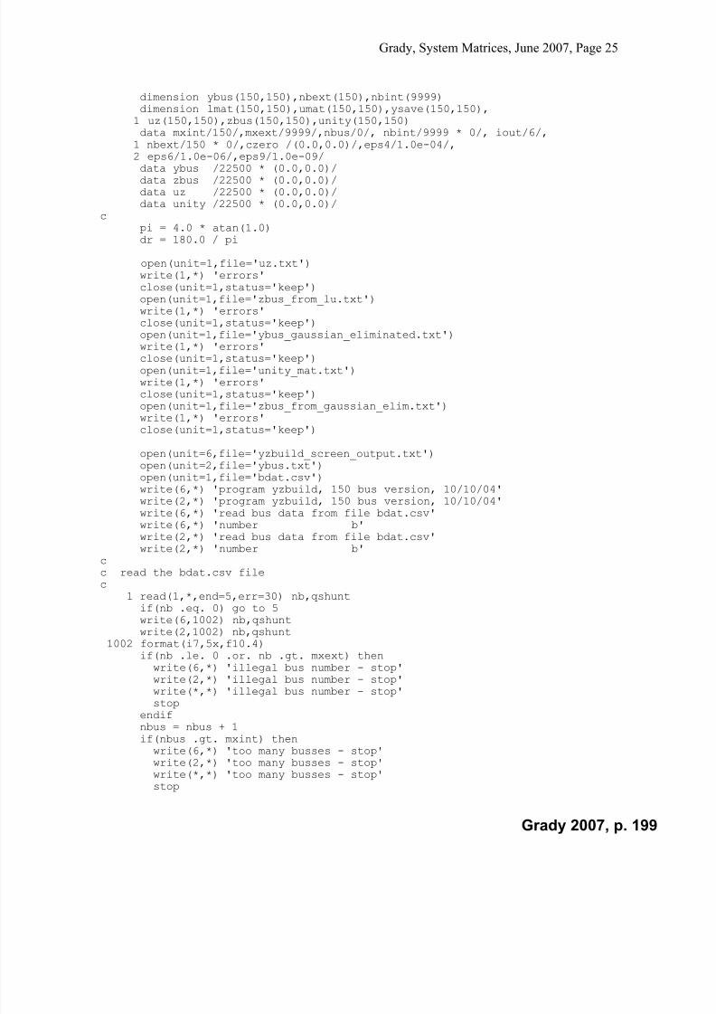
7/22/2019 Fundamentals Grady Notes June 2007 Print
http://slidepdf.com/reader/full/fundamentals-grady-notes-june-2007-print 199/388
Grady, System Matrices, June 2007, Page 25
dimension ybus(150,150),nbext(150),nbint(9999)dimension lmat(150,150),umat(150,150),ysave(150,150),1 uz(150,150),zbus(150,150),unity(150,150)data mxint/150/,mxext/9999/,nbus/0/, nbint/9999 * 0/, iout/6/,1 nbext/150 * 0/,czero /(0.0,0.0)/,eps4/1.0e-04/,2 eps6/1.0e-06/,eps9/1.0e-09/
data ybus /22500 * (0.0,0.0)/data zbus /22500 * (0.0,0.0)/data uz /22500 * (0.0,0.0)/data unity /22500 * (0.0,0.0)/
c pi = 4.0 * atan(1.0)
dr = 180.0 / pi
open(unit=1,file='uz.txt')write(1,*) 'errors'close(unit=1,status='keep')open(unit=1,file='zbus_from_lu.txt')write(1,*) 'errors'close(unit=1,status='keep')
open(unit=1,file='ybus_gaussian_eliminated.txt')write(1,*) 'errors'close(unit=1,status='keep')open(unit=1,file='unity_mat.txt')write(1,*) 'errors'close(unit=1,status='keep')open(unit=1,file='zbus_from_gaussian_elim.txt')write(1,*) 'errors'close(unit=1,status='keep')
open(unit=6,file='yzbuild_screen_output.txt')open(unit=2,file='ybus.txt')open(unit=1,file='bdat.csv')write(6,*) 'program yzbuild, 150 bus version, 10/10/04'
write(2,*) 'program yzbuild, 150 bus version, 10/10/04'write(6,*) 'read bus data from file bdat.csv'write(6,*) 'number b'write(2,*) 'read bus data from file bdat.csv'write(2,*) 'number b'
cc read the bdat.csv filec 1 read(1,*,end=5,err=30) nb,qshunt
if(nb .eq. 0) go to 5write(6,1002) nb,qshunt
write(2,1002) nb,qshunt1002 format(i7,5x,f10.4)
if(nb .le. 0 .or. nb .gt. mxext) thenwrite(6,*) 'illegal bus number - stop'write(2,*) 'illegal bus number - stop'write(*,*) 'illegal bus number - stop'stop
endifnbus = nbus + 1if(nbus .gt. mxint) thenwrite(6,*) 'too many busses - stop'write(2,*) 'too many busses - stop'write(*,*) 'too many busses - stop'stop
Grady 2007, p. 199

7/22/2019 Fundamentals Grady Notes June 2007 Print
http://slidepdf.com/reader/full/fundamentals-grady-notes-june-2007-print 200/388
Grady, System Matrices, June 2007, Page 26
endifnbext(nbus) = nbnbint(nb) = nbusycap = cmplx(0.0,qshunt)ybus(nbus,nbus) = ybus(nbus,nbus) + ycapgo to 1
5 close(unit=1,status='keep')
c open(unit=1,file='ldat.csv')
write(6,*)write(6,*) 'read line/transformer data from file ldat.csv'write(6,*) ' from to r x',1 ' b'write(2,*) 'read line/transformer data from file ldat.csv'write(2,*) ' from to r x',1 ' b'
cc read the ldat.csv filec 10 read(1,*,end=15,err=31) nfrom,nto,r,x,charge
if(nfrom .eq. 0 .and. nto .eq. 0) go to 15
write(6,1004) nfrom,nto,r,x,chargewrite(2,1004) nfrom,nto,r,x,charge1004 format(1x,i5,2x,i5,3(2x,f10.4)) if(nfrom .lt. 0 .or. nfrom .gt. mxext .or. nto .lt. 0
1 .or. nto .gt. mxext) thenwrite(6,*) 'illegal bus number - stop'write(2,*) 'illegal bus number - stop'write(*,*) 'illegal bus number - stop'stop
endifif(nfrom .eq. nto) thenwrite(6,*) 'same bus number given on both ends - stop'write(2,*) 'same bus number given on both ends - stop'write(*,*) 'same bus number given on both ends - stop'
stopendifif(r .lt. -eps6) thenwrite(6,*) 'illegal resistance - stop'write(2,*) 'illegal resistance - stop'write(*,*) 'illegal resistance - stop'stop
endif if(charge .lt. -eps6) then
write(6,*) 'line charging should be positive'write(2,*) 'line charging should be positive'write(*,*) 'line charging should be positive'stop
endifif(nfrom .ne. 0) thennfrom = nbint(nfrom)if(nfrom .eq. 0) thenwrite(6,*) 'bus not included in file bdat.csv - stop'write(2,*) 'bus not included in file bdat.csv - stop'write(*,*) 'bus not included in file bdat.csv - stop'stop
endif endif
if(nto .ne. 0) then nto = nbint(nto)
Grady 2007, p. 200
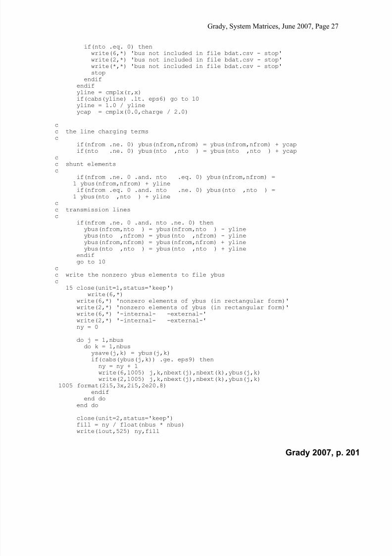
7/22/2019 Fundamentals Grady Notes June 2007 Print
http://slidepdf.com/reader/full/fundamentals-grady-notes-june-2007-print 201/388
Grady, System Matrices, June 2007, Page 27
if(nto .eq. 0) thenwrite(6,*) 'bus not included in file bdat.csv - stop'
write(2,*) 'bus not included in file bdat.csv - stop'write(*,*) 'bus not included in file bdat.csv - stop'stop
endif endif
yline = cmplx(r,x)if(cabs(yline) .lt. eps6) go to 10yline = 1.0 / ylineycap = cmplx(0.0,charge / 2.0)
cc the line charging termsc if(nfrom .ne. 0) ybus(nfrom,nfrom) = ybus(nfrom,nfrom) + ycap
if(nto .ne. 0) ybus(nto ,nto ) = ybus(nto ,nto ) + ycapcc shunt elementsc if(nfrom .ne. 0 .and. nto .eq. 0) ybus(nfrom,nfrom) =
1 ybus(nfrom,nfrom) + ylineif(nfrom .eq. 0 .and. nto .ne. 0) ybus(nto ,nto ) =1 ybus(nto ,nto ) + yline
cc transmission linesc if(nfrom .ne. 0 .and. nto .ne. 0) then
ybus(nfrom,nto ) = ybus(nfrom,nto ) - ylineybus(nto ,nfrom) = ybus(nto ,nfrom) - ylineybus(nfrom,nfrom) = ybus(nfrom,nfrom) + ylineybus(nto ,nto ) = ybus(nto ,nto ) + yline
endifgo to 10
c
c write the nonzero ybus elements to file ybusc 15 close(unit=1,status='keep')
write(6,*)write(6,*) 'nonzero elements of ybus (in rectangular form)'write(2,*) 'nonzero elements of ybus (in rectangular form)'write(6,*) '-internal- -external-'write(2,*) '-internal- -external-'ny = 0
do j = 1,nbusdo k = 1,nbusysave(j,k) = ybus(j,k)if(cabs(ybus(j,k)) .ge. eps9) thenny = ny + 1write(6,1005) j,k,nbext(j),nbext(k),ybus(j,k)write(2,1005) j,k,nbext(j),nbext(k),ybus(j,k)
1005 format(2i5,3x,2i5,2e20.8)endif
end doend do
close(unit=2,status='keep') fill = ny / float(nbus * nbus)
write(iout,525) ny,fill
Grady 2007, p. 201

7/22/2019 Fundamentals Grady Notes June 2007 Print
http://slidepdf.com/reader/full/fundamentals-grady-notes-june-2007-print 202/388
Grady, System Matrices, June 2007, Page 28
525 format(/1x,'number of nonzero elements in ybus = ',i5/1x,1'percent fill = ',2pf8.2/)
cc bifactorization - replace original ybus with luc nm1 = nbus - 1
do ipiv = 1,nm1write(iout,530) ipiv
530 format(1x,'lu pivot element = ',i5)ipiv1 = ipiv + 1alpha = 1.0 / ybus(ipiv,ipiv)do k = ipiv1,nbusybus(ipiv,k) = alpha * ybus(ipiv,k)
end dodo j = ipiv1,nbusalpha = ybus(j,ipiv)do k = ipiv1,nbusybus(j,k) = ybus(j,k) - alpha * ybus(ipiv,k)
end doend do
end do
write(iout,530) nbuswrite(iout,532)
532 format(/1x,'nonzero lu follows'/)open(unit=4,file='lu.txt')nlu = 0
do j = 1,nbusdo k = 1,nbusymag = cabs(ybus(j,k))if(ymag .gt. eps9) thennlu = nlu + 1write(iout,1005) j,k,nbext(j),nbext(k),ybus(j,k)
write(4,1005) j,k,nbext(j),nbext(k),ybus(j,k)endifend do
end do
fill = nlu / float(nbus * nbus)write(iout,535) nlu,fill
535 format(/1x,'number of nonzero elements in lu = ',i5/1x,1'percent fill = ',2pf8.2/)close(unit=4,status='keep')
cc check l times uc write(iout,560)560 format(1x,'lu .ne. ybus follows'/)
do j = 1,nbusdo k = 1,nbuslmat(j,k) = czeroumat(j,k) = czeroif(j .ge. k) lmat(j,k) = ybus(j,k)if(j .lt. k) umat(j,k) = ybus(j,k)
end doumat(j,j) = 1.0
end do
Grady 2007, p. 202

7/22/2019 Fundamentals Grady Notes June 2007 Print
http://slidepdf.com/reader/full/fundamentals-grady-notes-june-2007-print 203/388
Grady, System Matrices, June 2007, Page 29
do j = 1,nbusdo k = 1,nbusytest = czerodo l = 1,kytest = ytest + lmat(j,l) * umat(l,k)
end do
diff = ysave(j,k) - ytestif(cabs(diff) .gt. eps4) write(iout,1005) j,k,nbext(j),
1 nbext(k),diffend do
end docc form uz (urt + diag)c write(iout,536) nbus536 format(1x,'uz pivot = ',i5)
uz(nbus,nbus) = 1.0 / ybus(nbus,nbus)nm1 = nbus - 1
do kdum = 1,nm1
k = nbus - kdumwrite(iout,536) kuz(k,k) = 1.0 / ybus(k,k)kp1 = k + 1do j = kp1,nbusuzelem = czerojm1 = j - 1alpha = 1.0 / ybus(j,j)do l = k,jm1uzelem = uzelem - ybus(j,l) * uz(l,k)
end douz(j,k) = uzelem * alpha
end doend do
write(iout,537)537 format(/1x,'nonzero uz follows'/)
open(unit=8,file='uz.txt')nlu = 0
do j = 1,nbusdo k = 1,nbusymag = cabs(uz(j,k))if(ymag .gt. eps9) thennlu = nlu + 1write(iout,1005) j,k,nbext(j),nbext(k),uz(j,k)write(8,1005) j,k,nbext(j),nbext(k),uz(j,k)
endifend do
end do
fill = nlu / float(nbus * nbus)write(iout,545) nlu,fill
545 format(/1x,'number of nonzero elements in uz = ',i5/1x,1'percent fill = ',2pf8.2/)close(unit=8,status='keep')
cc form zc
Grady 2007, p. 203
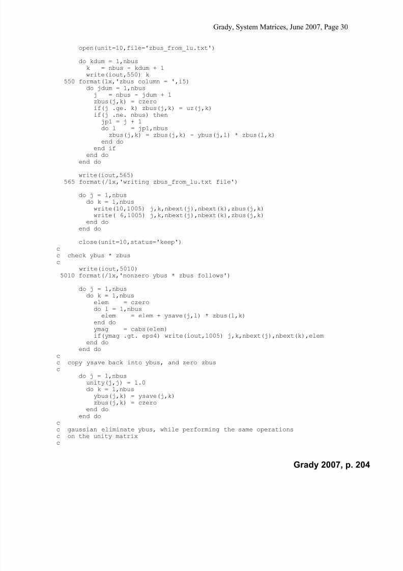
7/22/2019 Fundamentals Grady Notes June 2007 Print
http://slidepdf.com/reader/full/fundamentals-grady-notes-june-2007-print 204/388
Grady, System Matrices, June 2007, Page 30
open(unit=10,file='zbus_from_lu.txt')
do kdum = 1,nbusk = nbus - kdum + 1write(iout,550) k
550 format(1x,'zbus column = ',i5)do jdum = 1,nbus
j = nbus - jdum + 1zbus(j,k) = czeroif(j .ge. k) zbus(j,k) = uz(j,k)if(j .ne. nbus) thenjp1 = j + 1do l = jp1,nbuszbus(j,k) = zbus(j,k) - ybus(j,l) * zbus(l,k)
end doend if
end doend do
write(iout,565)565 format(/1x,'writing zbus_from_lu.txt file')
do j = 1,nbusdo k = 1,nbuswrite(10,1005) j,k,nbext(j),nbext(k),zbus(j,k)write( 6,1005) j,k,nbext(j),nbext(k),zbus(j,k)
end doend do
close(unit=10,status='keep')cc check ybus * zbusc write(iout,5010)5010 format(/1x,'nonzero ybus * zbus follows')
do j = 1,nbusdo k = 1,nbuselem = czerodo l = 1,nbuselem = elem + ysave(j,l) * zbus(l,k)
end doymag = cabs(elem)if(ymag .gt. eps4) write(iout,1005) j,k,nbext(j),nbext(k),elem
end doend do
cc copy ysave back into ybus, and zero zbusc do j = 1,nbus
unity(j,j) = 1.0do k = 1,nbusybus(j,k) = ysave(j,k)zbus(j,k) = czero
end doend do
cc gaussian eliminate ybus, while performing the same operationsc on the unity matrixc
Grady 2007, p. 204
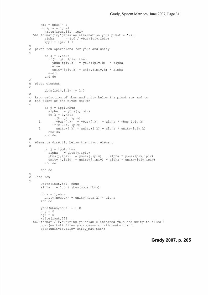
7/22/2019 Fundamentals Grady Notes June 2007 Print
http://slidepdf.com/reader/full/fundamentals-grady-notes-june-2007-print 205/388
Grady, System Matrices, June 2007, Page 31
nm1 = nbus - 1do ipiv = 1,nm1write(iout,561) ipiv
561 format(1x,'gaussian elimination ybus pivot = ',i5)alpha = 1.0 / ybus(ipiv,ipiv)
ipp1 = ipiv + 1c
c pivot row operations for ybus and unityc do k = 1,nbus
if(k .gt. ipiv) thenybus(ipiv,k) = ybus(ipiv,k) * alphaelseunity(ipiv,k) = unity(ipiv,k) * alpha
endifend do
cc pivot elementc ybus(ipiv,ipiv) = 1.0c
c kron reduction of ybus and unity below the pivot row and toc the right of the pivot columnc do j = ipp1,nbus
alpha = ybus(j,ipiv)do k = 1,nbusif(k .gt. ipiv)
1 ybus(j,k) = ybus(j,k) - alpha * ybus(ipiv,k)if(k .lt. ipiv)
1 unity(j,k) = unity(j,k) - alpha * unity(ipiv,k)end do
end docc elements directly below the pivot element
c do j = ipp1,nbusalpha = ybus(j,ipiv)ybus(j,ipiv) = ybus(j,ipiv) - alpha * ybus(ipiv,ipiv)unity(j,ipiv) = unity(j,ipiv) - alpha * unity(ipiv,ipiv)
end do
end docc last rowc write(iout,561) nbus
alpha = 1.0 / ybus(nbus,nbus)
do k = 1,nbus unity(nbus,k) = unity(nbus,k) * alpha
end do
ybus(nbus,nbus) = 1.0ngy = 0ngu = 0write(iout,562)
562 format(/1x,'writing gaussian eliminated ybus and unity to files')open(unit=12,file='ybus_gaussian_eliminated.txt')open(unit=13,file='unity_mat.txt')
Grady 2007, p. 205

7/22/2019 Fundamentals Grady Notes June 2007 Print
http://slidepdf.com/reader/full/fundamentals-grady-notes-june-2007-print 206/388
Grady, System Matrices, June 2007, Page 32
do j = 1,nbusdo k = 1,nbusymag = cabs(ybus(j,k))if(ymag .ge. eps9) thenwrite(12,1005) j,k,nbext(j),nbext(k),ybus(j,k)ngy = ngy + 1
endifumag = cabs(unity(j,k))if(umag .ge. eps9) thenwrite(13,1005) j,k,nbext(j),nbext(k),unity(j,k)ngu = ngu + 1
endifend do
end do
close(unit=12,status='keep')close(unit=13,status='keep')fill = ngy / float(nbus * nbus)write(iout,555) ngy,fill
555 format(/1x,'number of nonzero elements in gaussian eliminated',
1' ybus = ',i5/1x,1'percent fill = ',2pf8.2/)fill = ngu / float(nbus * nbus)write(iout,556) ngu,fill
556 format(/1x,'number of nonzero elements in gaussian eliminated',1' unity matrix = ',i5/1x,1'percent fill = ',2pf8.2/)
cc back substitute to find zc do k = 1,nbus
zbus(nbus,k) = unity(nbus,k)end do
do jdum = 2,nbusj = nbus - jdum + 1write(iout,550) jdo kdum = 1,nbusk = nbus - kdum + 1zbus(j,k) = unity(j,k)jp1 = j + 1do l = jp1,nbuszbus(j,k) = zbus(j,k) - ybus(j,l) * zbus(l,k)
end doend do
end do
write(iout,566)566 format(/1x,'writing zbus_from_gaussian_elim.txt file')
open(unit=11,file='zbus_from_gaussian_elim.txt')
do j = 1,nbusdo k = 1,nbuswrite(11,1005) j,k,nbext(j),nbext(k),zbus(j,k)write( 6,1005) j,k,nbext(j),nbext(k),zbus(j,k)
end doend do
close(unit=11,status='keep')
Grady 2007, p. 206

7/22/2019 Fundamentals Grady Notes June 2007 Print
http://slidepdf.com/reader/full/fundamentals-grady-notes-june-2007-print 207/388
Grady, System Matrices, June 2007, Page 33
cc check ybus * zbusc write(iout,5010)
do j = 1,nbusdo k = 1,nbus
elem = czerodo l = 1,nbuselem = elem + ysave(j,l) * zbus(l,k)
end doymag = cabs(elem)if(ymag .gt. eps4) write(iout,1005) j,k,nbext(j),nbext(k),elem
end doend do
stop30 write(iout,*) 'error in reading bdat.csv file - stop'
write(*,*) 'error in reading bdat.csv file - stop'stop
31 write(iout,*) 'error in reading ldat.csv file - stop'
write(*,*) 'error in reading ldat.csv file - stop'stop
end
Grady 2007, p. 207

7/22/2019 Fundamentals Grady Notes June 2007 Print
http://slidepdf.com/reader/full/fundamentals-grady-notes-june-2007-print 208/388
Fortran program yzbuild.f (and executable yzbuild.exe) reads bus datafile bdat.csv, and line/transformer data file ldat.csv, and then producesthe corresponding impedance matrix using LU decomposition, and again usingGaussian elimination. The program is dimensioned for systems as large as150 busses.
Comma-separated file bdat.csv contains the bus data, using the format:bus number , shunt q (in pu, where capacitance positive, and inductanceis negative)
Comma-separated file ldat.csv contains the branch data, using the format:from bus number , to bus number , r(pu) , x(pu) , line charging (in pu,for the total length of line)
It is OK to have ties to ground in ldat.csv. Ground is bus = 0.
Two sample systems are included. One has three busses, and the other haseighty-three busses. To try out yzbuild, simply copy and rename the datafiles for either system as bdat.csv and ldat.csv, and then click on yzbuild.exe.
Grady 2007, p. 208

7/22/2019 Fundamentals Grady Notes June 2007 Print
http://slidepdf.com/reader/full/fundamentals-grady-notes-june-2007-print 209/388
The data below are given in per unit. R and X are the series impedances of the transmission lines
(in per unit ohms), and B is the line charging of the transmission lines (in per unit mhos).
Build the Y matrix. Show the complex terms individually. Do not perform any complex
arithmetic such as inversions, and do not combine the terms.
From Bus To Bus R – pu ohms jX – pu ohms jB – pu mhos
1 2 0.004 j0.053 j0
2 3 0.02 j0.25 j0.22
3 4 0.02 j0.25 j0.22
2 4 0.01 j0.15 j0.11
Grady 2007, p. 209
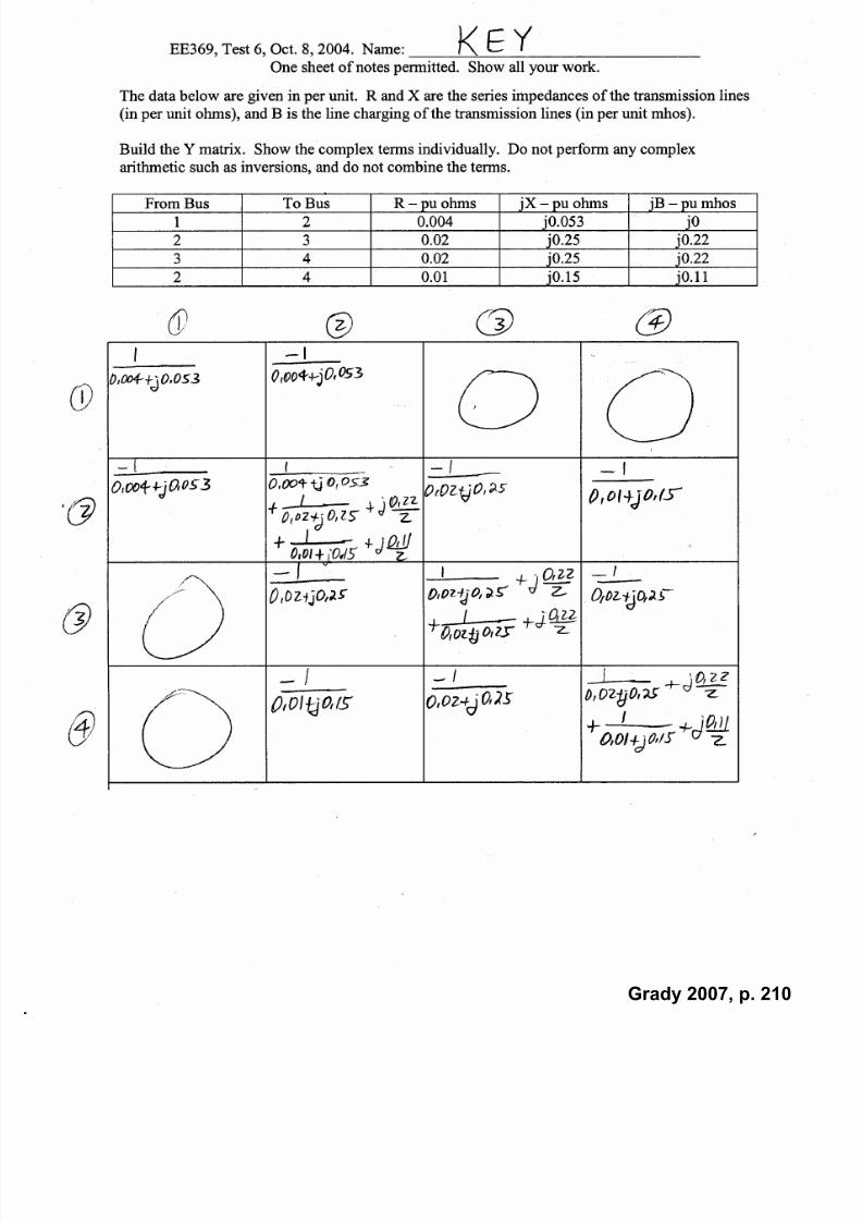
7/22/2019 Fundamentals Grady Notes June 2007 Print
http://slidepdf.com/reader/full/fundamentals-grady-notes-june-2007-print 210/388
Grady 2007, p. 210

7/22/2019 Fundamentals Grady Notes June 2007 Print
http://slidepdf.com/reader/full/fundamentals-grady-notes-june-2007-print 211/388
Use the definition of Z-matrix elements to find matrix elements z11, z12, z13, z14.
j21 2 3 4
j8
j6
j5
j4
j4
Grady 2007, p. 211

7/22/2019 Fundamentals Grady Notes June 2007 Print
http://slidepdf.com/reader/full/fundamentals-grady-notes-june-2007-print 212/388
Grady 2007, p. 212

7/22/2019 Fundamentals Grady Notes June 2007 Print
http://slidepdf.com/reader/full/fundamentals-grady-notes-june-2007-print 213/388
Grady, Programming Consideration, June 2007, Page 1
Programming Considerations
Methods for efficient programming. Sparsity techniques. Optimal bus ordering.
1. Sparsity Programming
Many power system matrices tend to be very large and very sparse. A typical example is the
admittance matrix Y . Each diagonal element of Y is non-zero, and each branch connected
between busses occurs twice in Y , so that a branch between busses j and k appears in y j k , and
yk j, . Additional parallel branches and shunt elements do not create additional y elements.
Consider a power system with 250 busses and 750 branches. Assume that none of the branches
are parallel branches. The dimension of Y is 250 x 250, or 62,500 elements. However, the
number of non-zero terms in Y equals 250 + 2(750), or 1750. Therefore, only 2.8% of the Y
elements are non-zero. The savings are even more impressive for larger systems, since Y grows
by N 2
, but the number of non-zero terms grows by N . For example, a 2500 bus, 7500 branch Yhas only 0.28% non-zero terms.
In most cases, the coding of large computer programs involves trade-offs between execution
time and memory requirements. Sparsity storage techniques, however, reduce both execution
time and memory requirements. The only drawback of sparsity programming is that it is more
difficult to code than full-matrix programming.
There are several techniques for sparsity programming. The method presented here is known as
the sequential trace method, and although the example is given for Y , it applies equally well to
the loadflow Jacobian matrix.
Four vectors are used for storing and accessing the sparse Y :
1. Instead of storing Y as a square matrix of dimension N x N , Y is stored as a column
vector, whose length M is estimated (at the time of program compilation) using typical
sparsity ratios of 1% - 5% of N x N . The location from the top of Y is known as the stack
location.
2. Vector NFIRST , of length N , points to the stack location in Y of the first non-zero element
of a row (in column order). For example, the stack position of the first non-zero element
in Row k is found in NFIRST(k).
3. Vector NCOL, of length M , gives the Y column number of the associated Y stack position.
4. Vector NEXT , of length M , gives the stack location in Y of the next non-zero element in
the corresponding row. A zero value indicates the end of the row.
The term "sequential trace" is derived from the fact that all elements of a Y row can be found, in
a column-order sequence, by starting with the lowest occupied column number of the row, and
continuing through the highest occupied column number of the row.
Grady 2007, p. 213

7/22/2019 Fundamentals Grady Notes June 2007 Print
http://slidepdf.com/reader/full/fundamentals-grady-notes-june-2007-print 214/388
Grady, Programming Consideration, June 2007, Page 2
As an example, let Row 23 of Y have three elements: y235, in stack location 987, y23 23, in stack
location 560, and y23138, in stack location 1230. These elements can be found as follows:
1. The stack location of the first non-zero element (in column order) of Row 23 is found by
looking in NFIRST (23). In this example, NFIRST (23) equals 987.
2. The corresponding column number is found in NCOL(987), which equals 5. Thus, the
equivalent Y (23,5) element is found in stack position Y (987).
3. The stack position of the next non-zero Y element in Row 23 is found by looking at
NEXT (987). The value of NEXT (987) is 560.
4. The corresponding column number is found in NCOL(560), which equals 23. Thus, the
equivalent Y (23,23) element is found in stack position Y (560).
5. The stack position of the next non-zero Y element in Row 23 is found by looking at
NEXT (560). The value of NEXT (560) is 1230.
6. The corresponding column number is found in NCOL(1230), which equals 138. Thus,
the equivalent Y (23,138) element is found in stack position Y (1230).
7. A zero in NEXT (1230) indicates that the end Row 23 has been reached.
Table 1 gives the corresponding numbers for this example.
Table 1: Example of Sequential Trace Method for Sparsity Storage, where the First Non-Zero
Column for Row 23 is found in NFIRST (23) = 987
valuey01381230
valuey5605987
valuey123023560
NEXT NCOLLocationStack
23,138
23,5
23,23
Y
When Y is first built, the elements for each row are contiguous. However, as Y is Gaussianeliminated or LU decomposed, "fill-ins" are created, and they are normally added to the end of
the Y stack. The four vectors must be modified appropriately, and the elements of a row are no
longer contiguous.
Note - if Y is to be Gaussian eliminated, this can be performed simultaneously while Y is being
formed in row order, thereby never saving the LLT part of the eliminated Y matrix. For
example, Row 1 is formed and saved. Next, Row 2 is formed, then Gaussian eliminated by Row
Grady 2007, p. 214

7/22/2019 Fundamentals Grady Notes June 2007 Print
http://slidepdf.com/reader/full/fundamentals-grady-notes-june-2007-print 215/388
Grady, Programming Consideration, June 2007, Page 3
1, and then saved. Next, Row 3 is formed, eliminated by Row 1, then by Row 2, and then saved,
etc.
2. Optimal Bus Ordering
Gaussian elimination and LU decomposition reduce matrices through a series of row operations.
Once the decision has been made to use sparsity programming, then it is very important in power
system applications to order the busses efficiently so that the advantages of sparsity
programming are not nullified by the creation of too many "fill-ins" (i.e. zero elements that
become non-zeros).
Consider the simple five-bus system given figuratively in Figure 1.
12
3
4
5
Figure 1. Simple Five-Bus System
The form of Y , for the given bus order, is
x x
x x x
x x x
x x
x x x x x
,
and the final form of the Gaussian eliminated Y is a full (URT+D) matrix, or
x x
x x
x
x x x x x
,
where the terms are "fill-ins."
However, if the bus numbers for busses 1 and 5 are interchanged, then the initial Y has the form
Grady 2007, p. 215

7/22/2019 Fundamentals Grady Notes June 2007 Print
http://slidepdf.com/reader/full/fundamentals-grady-notes-june-2007-print 216/388
Grady, Programming Consideration, June 2007, Page 4
x x x x x
x x x
x x x
x x
x x
,
and the final form of the Gaussian eliminated Y is
x
x x
x x x
x x
x x
,
which has no fill-ins.
While this is a simple example, the importance of bus ordering cannot be overstated. Of course,
an efficient computer code does not require the user to order the busses ahead of time. Rather,
the user simply inputs his/her desired bus numbers, in no particular order, and the program
develops an "internal" (to the program) bus order. The following three methods are often used:
Method 1: Before Gaussian elimination begins, order the busses according to the number of
connected branches, ignoring parallel branches and shunt elements, so that the busses
with the fewest branches are first, and the busses with the most branches are last.
Method 2: Order the busses so that after each step of Gaussian elimination, the next bus in theorder is the one that has the fewest branches, including intermediate fill-in branches.
Method 3: Order the busses so that after each step of Gaussian elimination, the next bus in the
order is the one that creates the fewest fill-ins. This requires a simulated row-
reduction for all candidate busses.
Method 1 is the simplest and provides the highest incremental benefit. Method 2 usually
provides the best overall speed and memory benefits. Method 3 is more time-consuming to
compute, and the time and storage savings gained by Method 3 usually do not offset its
additional ordering computation time.
The impact of optimal ordering on the Gaussian elimination of Y for six sample systems is
shown in Table 2.
Grady 2007, p. 216

7/22/2019 Fundamentals Grady Notes June 2007 Print
http://slidepdf.com/reader/full/fundamentals-grady-notes-june-2007-print 217/388
Grady, Programming Consideration, June 2007, Page 5
Table 2: Impact of Optimal Bus Ordering Methods on Gaussian Elimination of Y
Elements in ------------ Elements in Gaussian-Eliminated Y ------------
System in Y User Bus Order Method 1 Method 2 Method 3
18 Bus 52 66 41 35 35
83 Bus 303 592 292 264 267
125 Bus 421 1,357 614 419 422
264 Bus 976 5,736 1,204 1,005 1,004
515 Bus 1,761 14,142 1,992 1,763 1,751
2245 Bus 8,257 94,468 25,775 9,473 9,218*
* Estimated using similar results for loadflow Jacobian matrix
The impact of optimal bus ordering on the Jacobian matrix, before and after Gaussian
elimination, is shown in Figures 2a, 2b, and 2c, which correspond to optimal ordering methods 1,2, and 3, respectively.
Grady 2007, p. 217

7/22/2019 Fundamentals Grady Notes June 2007 Print
http://slidepdf.com/reader/full/fundamentals-grady-notes-june-2007-print 218/388
Grady, Programming Consideration, June 2007, Page 6
°° °°°° °°°° °°°° °°°° °°°° °°
°° °°°° °°°° °°°° °°°° °°°° °°°° °°
°° °°°° °°°° °°°° °°°° °°°° °°°° °°°° °°
°° °°°° °°°° °°°° °°°° °°°° °°°° °°
°° °°°° °°°° °°°° °°°° °°°° °°°°°° °°
°°°° °°°°°° °°°°°° °°°°°° °°°°°° °°°°°° °°
°°°° °°°°°° °°°°°° °°°°°°°°°°°°°°°°°° °°°°°° °°
°°°° °°°°°° °°°°°°°°°°°°°°°°°° °°
°°°° °°°° °°°°°° °°°°°°°° °°°°°° °°°°°° °°°°°° °°
°°°° °°°°°° °°°°°°°°°°°°°°°°°°°°°°°°°°
°° °°°°°° °°°°°°°° °°°°°° °°
°°°°°°°°°°°°°°°°°°°°°°°°°°°°°°°°°°°°°°°° °°°°°° °°°°°° °°
°°°° °°°°°°°°°°°°°°°° °°°°°° °°°°°° °°°°
°° °°°°°° °° °°°° °° °°°°°° °°°°°° °°°° °°°°°° °°°°
°° °° °°°° °° °°°° °° °°°° °° °°°°°° °°°°°° °°°° °°°°°° °°°°
°°°° °°°°°° °°°°°°°°°°°°°°°° °°°°°° °°°°°° °° °°
°° °° °°°°°° °°°°°° °°°°°° °°°°°° °°°° °° °°°° °° °°°°°° °°
°°°° °°°° °°°°°° °°°°°° °°°°
°° °°°°°° °°°°°° °°°°°°°° °°°°°° °°°°°° °°°°°° °°
°°°° °°°°°° °°°°°°°°°°°°°°°°°° °°°°°° °°
°° °°°°°° °°°°°° °° °°°° °° °°°°°° °°°°°° °°°° °°°°
°° °°°°°° °° °°°° °° °°°°°° °° °°°°°° °° °°°° °° °°°°°° °° °°°°
°°°°°° °°°°°°°° °°°° °°°° °°°° °°°° °°°° °° °° °°
°° °° °° °°°°°° °° °°°°°° °° °°°°°° °° °°°°°° °° °°°°°° °° °°°°°° °° °°
°°°° °° °°°°°° °° °°°° °°°° °°°° °°°° °°°° °°°° °°
°° °°°° °°°° °°°° °°°° °°°° °°°°°° °° °°°°°° °° °°°° °°°° °°°° °°°° °°
°° °°°° °°°° °°°° °°°° °°°° °°°° °°°° °°°°°° °° °°°°°° °° °°°°°° °° °°
°°°° °° °°°° °°°° °°°° °°°° °°°° °°°° °°°° °°°° °°°°°° °° °°°°°° °° °°°° °° °° °°°° °° °° °°
°° °° °° °°°° °° °° °°°° °°°° °°°° °°°° °°°° °°°°°°°° °°°°°°°° °°°° °°
°° °°°° °°°° °°°° °°°° °°°° °°°° °°°° °°°° °°°° °°
°° °°°° °°°° °°°° °°°° °°°° °°°° °°°° °°°° °° °°°°°° °° °°°°°° °° °° °°
°° °° °° °°°° °° °°°°°° °° °°°°°° °° °°°°°° °° °°°°°° °°°° °°
°° °°°° °°°° °°°°°°°° °°°°°°°° °°°° °°°° °°°° °°°° °° °°°°°° °° °°°°
°°°°°°°°°°°°°°°°°°°° °°°°°°°° °°°°°° °°°°°°°° °°°°°°°° °°°° °°
°° °°°° °°°° °°°° °°°° °°°° °°°° °°°°°°
°° °°°°°°°° °° °°°°°° °° °°°°°° °° °° °°°° °° °° °°°°°° °° °°°°°° °° °°
°°°° °° °°°°°° °° °°°° °°°° °°°° °°°° °°°° °°°° °° °°°° °°°° °° °°°°°° °° °° °°
°°°° °° °° °°°° °° °° °° °° °°°° °° °° °° °° °°°° °° °° °° °° °° °° °°
°° °° °° °° °° °° °° °°
250
200
150
100
50
0
0 50 100 150 200 250
Column
°° °°° °°°° °°° °°°° °°° °°
°° °°° °°°° °°° °°°° °°
° °°°° °°° °°°° °°° °°°° °°
° °°°° °°° °°°° °°° °°°° °°
° °°°° °°° °°°° °°° °°°° °°° °°
°° °°° °°°° °°° °°°°°° °°°°° °°°° °° °°
° °° °°°°°° °°°°° °°°° °°°°° °°°°°°°° °°
°°° °°°°°° °°°°° °°°° °°°°° °°°°°°°° °°°°° °°
°°°° °°°°° °°°° °°°°° °°°°°° °°°°° °°°°
°°°° °°°°° °°°° °° °°° °° °°°°°° °°
°°° °°°°°° °°°°° °°°°°° °°°°° °°°° °°° °°
°°°° °°°°° °°°°°° °°°°° °°°°°° °°°°° °°
°°°° °°°°° °°°° °° °°° °° °°°°°° °°°°° °°°°°° °°
°°° °°°° °°° °°°° °°°°° °°°°°° °°° °°
°°°° °°°°° °°°° °°° °°°° °° °°
° °° °°°° °°° °°°°°° °°°°° °°°° °°° °°
°°°° °°°°° °°°°°° °°°°° °°°° °°
° °°°° °° °°° °° °°°°°° °°°°° °°°° °°°°° °°°°°° °°° °°°°°° °°°°° °°
°° °°° °°°° °°°°° °°°°°° °°°°° °°°°
°°°° °°°°° °°°° °° °°° °° °°°°°° °°°°° °°°°°° °°
°°° °°°° °° °°° °° °°°° °°°°° °°°°°° °°° °°
°°°° °°°°° °°°° °°° °°
°° °° °°° °° °°°°°° °° °°°°° °° °°°°°° °° °°°°° °° °°°°°° °° °° °°
°°° °° °° °°°° °° °° °° °°° °° °° °° °°°°°° °°°°° °°°°°° °° °°
°°° °° °°°°°° °° °° °°°°° °° °° °°°° °° °° °° °° °°° °° °° °° °° °°°°°° °°°°° °°
°° °°° °°°°°° °° °°°°° °° °°°° °° °° °°° °° °° °°°°°° °° °°
°°° °° °°°° °° °°° °° °°°°°° °° °°
°°° °° °°°°°° °° °° °°°°° °° °° °°°°°° °° °° °° °°°°° °° °° °° °°°° °° °° °° °° °° °°° °° °° °° °° °° °°
°°°° °° °°°°° °° °°°°°°°° °° °°°°°°° °° °°°°°° °° °° °°°°° °° °° °°
°° °° °° °° °° °° °° °° °°° °° °° °° °° °° °° °° °°°° °° °° °° °°° °° °° °° °°°°°° °° °° °° °° °°°°° °° °° °° °° °°°°°°°°°°°°°°°°°° °° °° °° °° °°
°°°°°°°°°°°°°°° °° °° °° °° °°°°°°°°°°°°°°°° °° °° °° °°°° °° °°°°°°°°°°°°°°°°° °° °° °° °°°° °° °°°°°°°°°°°°°°°° °° °° °° °°°° °° °° °°°°°°°°°°°°°°° °° °° °° °°°° °° °° °°°°°°°°°°°°°° °° °° °° °°°° °° °°°°°°°°°°°°°°°°° °° °° °° °°°° °° °°°°°°°°
°°°°°°°° °° °° °° °°°° °° °°°°°°°°°°°°°°° °° °° °° °°°° °° °°°°°°°°°°°°°° °° °° °° °°°° °° °° °°°°°°°°°°°°° °° °° °° °°°° °° °° °°°°°°°°°°°° °° °° °° °°°° °° °°°° °°°°°°°°°°° °° °° °° °°°° °° °°°° °°°°°°°°
°° °° °° °° °°°° °° °°°° °°°°°°°°° °° °° °° °°°° °° °°°° °°°°°°°°°° °° °° °°°° °°° °° °° °°°° °°°° °° °° °°°° °°°°°°°°°° °°°°°°°°° °° °° °°°° °°°°°°°°°° °°°°°°°°°°°°°° °° °°°° °°
°°°°° °° °°°° °°°°°°°° °°°°°° °°°°°°°°°°°°°°°°°°°°°°°°° °°°°°° °°°°°°°°°°°°°°°°°°°°°°°°°°°°°°°° °°°°°°°°°°°°°°°°°°°°°°°°°°°°°°° °°°°°°°°°°°°°°°°°°°°°°°°°°°°°° °°°°°°°°°°°°°°°°°°°°
°°°°°°°°° °°°°°°°°°°°°°°°°°°°°°°°°°°°° °°°°°°°°°°°°°°°°°°°°°°°°°°° °°°°°°°°°°°°°°°°°°°°°°°°°° °°°°°°°°°°°°°°°°°°°°°°°°° °°°°°°°°°°°°°°°°°°°°
°°°°°°°°°°°°°°°°°°°°°°°°°°°°°°°°°°°°°°°°°°°°°°°°°°°°°°°°°°°°°°°°°°°°°°°°°°°°°°°°°°°°°°°°°°°°°°°°°°°°°°°°°°°°°°°°°°°°°°°°°°°°°°°°°°°°°°°°°°°°°°°°°°°°°°°°°°°°°°°°°
°°°°°°°°°°°°°°°°°°°°°°°°°°°°°°°°°°°°°°°°°°°°°°°°°°°°°°°°°°°°°°°°°°°°°°°°°°°°°°°°°°°°°°°°°°°°°°°°°°°
°°°°°°°°°°°°°°°°°°°°°°°°°°°°°°°°°°°°°°°°°°°°°°°°°°°°°°°°°°°°°°°°°°°°°°
°°°°°°°°°°°°°°°°°°°°°
250
200
150
100
50
0
0 50 100 150 200 250
Column
Figure 2a. Jacobian Matrix for 125 Bus System, Before and After Gaussian Elimination, Using
Optimal Ordering Method 1
Grady 2007, p. 218

7/22/2019 Fundamentals Grady Notes June 2007 Print
http://slidepdf.com/reader/full/fundamentals-grady-notes-june-2007-print 219/388
Grady, Programming Consideration, June 2007, Page 7
°° °°°° °°°° °°°° °°°° °°°° °°
°°°°°°°°°°°°°°°°°°°°°°°°°°°°°°°°°°°°°°
°°°°°°°°°° °°°°°° °°°°°°°°°°°°°°°°°°°°°°°°°°°°°°°°°°°°°° °°°°°° °°
°° °°°° °°°°°°°°°°°°°°°°°°°°°°°° °°°°°°
°° °°°°°°°°°°°°°°°°°°°° °°°°°°°° °°°°°°°°°°°°
°°°°°°°°°°°°°°°°°°°°°°°°°°°°°°°°°°°°°°°°°°
°°°° °°°°°° °°°°°°°°°°°°°°°°°°°°°°°°°° °°°°°° °°°°°°
°°°°°°°° °°°°°° °°°°°°°°°°°°°°°°°°°°°°
°°°° °°°°°° °°°°°°°°°°°°°°°°°°°°°°°°°°°°
°°°°°°°°°° °°°°°° °°
°° °°°° °°°°°°°°°°°°°°°°°°°°°°°° °°°°°°°° °°°°°°°°°°°°
°°°°°°°°°° °°°°°° °°°°°°°°°°°°°°°°°°°°°°°°°° °°°°°° °°
°°°°°°°°°°°° °°°°°° °°°°°°°°°°°°°°°°°°°°°°°°°° °°°°°° °°°° °°
°° °°°°°° °°°°°° °°°°°° °°°°°° °°°°°° °°°°°° °°°°°°°°
°°°°°°°° °°°° °°°° °°°° °°°° °° °° °°°° °° °° °°°° °°°° °°°° °°°° °°
°°°°°°°°°°°°°°°°°°°°°°°°°°°° °°
°°°° °°°°°° °°°°°° °°°°°°°°°°°°°°°°°° °°°°°° °°
°° °° °°°° °° °°°°°° °°°°°° °°°°°° °°°°°° °°
°° °° °°°° °° °°°° °° °° °°°° °° °° °°°°°° °°°°°° °°°° °°°° °°
°° °°°° °°°° °° °°°° °° °°°° °° °°°° °° °°°°°° °°°°°° °°°°°° °°°°°° °°
°°°° °°°°°° °°°°°°°°°°°°°°°°°° °°°°°° °°
°°°° °°°°°° °°°° °°°° °°°° °°°° °°°° °° °° °°°° °° °° °°°° °°°°
°° °°°°°°°° °° °°°°°° °° °°°°°° °° °°°°°° °° °°°°°° °° °°
°°°° °° °°°°°° °° °°°°°° °° °°°° °° °° °°°° °° °° °°°°°° °° °°°°°° °° °°
°° °° °° °°°° °° °° °°°° °° °° °°°° °° °° °°°° °° °° °°°° °° °° °°
°° °° °° °°°° °° °° °°°° °° °° °°°° °° °° °°°° °° °° °°°° °° °° °°
°° °° °° °°°° °° °° °°°° °° °° °°°° °° °° °°°° °° °° °°°° °° °° °°°° °° °° °°
°° °° °° °°°° °° °° °°°° °° °° °°°° °° °°°°°° °° °°°°
°° °°°° °°°° °°°° °°°° °°°° °°°° °°°° °°°° °° °°°°°° °° °°°°°° °°°° °° °°
°° °°°° °° °°°° °° °° °°°° °° °° °°°°°° °° °°°°°° °° °°°° °° °° °° °° °° °° °°
°° °° °° °° °° °° °° °°°°°° °° °°°°°° °° °°°°°° °° °°°°°° °° °°°°°° °° °°°°°° °° °°
°°°° °° °°°°°° °° °°°° °° °° °°°° °° °° °°°° °°°° °°°° °°°° °°°° °° °° °°
°° °° °° °°°° °° °° °°°° °° °° °°°° °° °° °° °° °°
°° °° °° °° °° °°°°°° °° °°°°°° °° °°°° °° °° °°°° °° °° °°°° °° °° °°°° °° °° °°
°° °° °° °°°° °° °° °°°° °°°° °°°° °°°° °°°° °° °° °°°° °° °° °°°°°°°° °°
°°°°°° °°°° °° °° °°°° °° °° °°°°°° °° °° °°
°°°° °° °° °°
250
200
150
100
50
0
0 50 100 150 200 250
Column
°° °°° °°°° °°° °°°° °°° °°
°°°°°°°°°°°°°°°°°°
°°°°°°°°°°°° °°° °°°°°°
°°°°°°°°°°°°°°°°°°° °°
° °°°° °°° °°°°°°°°°°°°°°°°
°°°°°°°°°°°°°°°°°°°°°°°°°
°°°°°°°°°°°°°°°°°°°°°
°°°°° °°° °°°°°°°°°°°°°°°°
°° °°° °°°°°°°°°°° °°° °°
°°°°°°°°°°°°°°°° °°
° °°°°°°°°°°°°°°°°°°°°°°°
°° °°° °°°° °°° °°°°°°°°°
°°°°°°°°°°°°°°°°°°°°°°° °°
° °°°°°°°°°°°°°°°°°° °°
° °°°°°°°°°°° °°° °°°°°°
°°°°°°°°°°°° °°° °°°° °°° °°
°°°° °°°°° °°°° °° °°° °° °°°°°° °°
°°° °°°°°° °°°°° °°°° °° °°° °° °°°° °° °°° °° °°°°°° °°°°° °°°°°° °°°°° °°
°°°° °°°°° °°°° °° °°° °° °°°°°° °°°°° °°
°°°° °°°°° °°°° °° °°° °° °°°° °° °°° °° °°°°°° °°
°°° °°°° °° °°° °° °°°° °° °°° °° °°°° °° °°° °° °°
°°°° °°°°° °°°° °° °°° °° °°
°° °° °°° °° °°°° °° °°° °° °°°°°° °°°°° °°°° °° °°
° °° °°°°°° °°°°° °°°°°° °°°°° °°°° °° °°
° °° °°°°°° °°°°° °°°° °° °°° °° °°°° °° °°° °° °°
°° °°°°° °°°°°° °° °°°°° °° °°°°°° °° °° °°° °° °° °°°° °° °° °°
° °° °° °°°° °° °° °°° °° °° °°°° °° °° °°
° °° °° °°°° °° °° °°° °° °° °°°° °° °° °°° °° °° °°°° °° °° °°° °° °° °°
°° °° °° °°° °° °° °°°° °° °° °°° °° °° °°°° °° °° °°° °° °° °°
°° °° °° °°° °° °° °°°° °° °° °°° °° °° °°°° °° °° °°° °° °° °°°° °° °° °°
° °° °° °°°° °° °° °°° °° °° °°°° °° °° °°° °° °° °°°° °° °°°°° °° °°°°
°° °°°° °°° °°°° °°°° °° °° °° °°° °° °° °° °°°°°° °° °° °°°°° °° °° °°
°° °° °° °° °°° °° °° °° °°°° °° °° °° °°° °° °° °° °°°° °° °°°° °°°°° °° °°°° °°°°°° °° °° °°
° °° °° °°°° °° °° °° °°°°° °° °° °° °°°°°° °°°° °° °°°°° °°°° °° °°°°°° °° °°°°°° °°
° °° °°°°°° °°°° °° °° °°°°°° °°° °° °° °°°°°° °°°° °° °°°°°°°° °°° °° °°°°°°°° °°
°° °°°°°° °°°°°°°°° °°°°°° °°°°°°°°°° °°°°°°°°°°°° °° °°° °°°°°°°°°°°° °° °°°°°°°° °°°°°°°°°°°°°°°°° °°°°°°°°°°°°°°°°°°°°°°°°°°°°°°°°
°°°°°°°°°°°°°°°°°°°°°°°°°°°°°°°°°°°°°°°°°°°°°°°°°°°°°°°°°°°°°°°°°°°°°°°°°°°°°°°°°°°°°°°°°°°°°°°°°°°
°°°°°°°°°°°°°°°°°°°°°°°°°°°°°°°°°°°°°°°°°°°°°°°°°°°°°°°°°°°°°°°°°°°°°°
°°°°°°°°°°°°°°°°°°°°°
250
200
150
100
50
0
0 50 100 150 200 250
Column
Figure 2b. Jacobian Matrix for 125 Bus System, Before and After Gaussian Elimination, Using
Optimal Ordering Method 2
Grady 2007, p. 219

7/22/2019 Fundamentals Grady Notes June 2007 Print
http://slidepdf.com/reader/full/fundamentals-grady-notes-june-2007-print 220/388
Grady, Programming Consideration, June 2007, Page 8
°° °°°° °°°° °°°° °°°° °°°° °°
°°°°°°°°°°°°°°°°°°°°°°°°°°°°°°°°°°°°°°
°°°°°°°°°° °°°°°° °°°°°°°°°°°°°°°°°°°°°°°°°°°°°°°°°°°°°° °°°°°° °°
°° °°°° °°°°°°°°°°°°°°°°°°°°°°°° °°°°°°
°° °°°°°°°°°°°°°°°°°°°° °°°°°°°° °°°°°°°°°°°°
°°°°°°°°°°°°°°°°°°°°°°°°°°°°°°°°°°°°°°°°°°
°°°° °°°°°° °°°°°°°°°°°°°°°°°°°°°°°°°° °°°°°° °°°°°°
°°°°°°°° °°°°°° °°°°°°°°°°°°°°°°°°°°°°
°°°° °°°°°° °°°°°°°°°°°°°°°°°°°°°°°°°°°°
°°°°°°°°°° °°°°°° °°
°° °°°° °°°°°°°°°°°°°°°°°°°°°°°° °°°°°°°° °°°°°°°°°°°°
°°°°°°°°°° °°°°°° °°°°°°°°°°°°°°°°°°°°°°°°°° °°°°°° °°
°°°°°°°°°°°° °°°°°° °°°°°°°°°°°°°°°°°°°°°°°°°° °°°°°° °°°° °°
°° °°°°°° °°°°°° °°°°°° °°°°°° °°°°°° °°°°°° °°°°°°°°
°°°°°°°° °°°° °°°° °°°° °°°° °° °° °°°° °° °° °°°° °°°° °°°° °°°° °°
°°°°°°°°°°°°°°°°°°°°°°°°°°°° °°
°°°° °°°°°° °°°°°° °°°°°°°°°°°°°°°°°° °°°°°° °°
°° °° °°°° °° °°°°°° °°°°°° °°°°°° °°°°°° °°
°° °° °°°° °° °°°° °° °° °°°° °° °° °°°°°° °°°°°° °°°° °°°° °°
°° °°°° °°°° °° °°°° °° °°°° °° °°°° °° °°°°°° °°°°°° °°°°°° °°°°°° °°
°°°° °°°°°° °°°°°°°°°°°°°°°°°° °°°°°° °°
°°°° °°°°°° °°°° °°°° °°°° °°°° °°°° °° °° °°°° °° °° °°°° °° °°°°
°° °° °°°°°°°° °° °°°°°° °° °°°° °° °° °°°° °° °° °°°° °°°°
°° °°°°°°°° °° °°°°°° °° °°°°°° °° °°°°°° °° °°°°°° °° °°°°°° °° °°
°°°° °° °°°°°° °° °°°° °° °° °°°° °° °° °°°° °° °° °°°° °° °° °°
°° °° °° °°°° °° °° °°°°°°°° °°°°°°°° °°°° °° °°°°°° °° °°°°
°° °° °° °°°° °° °° °°°° °° °° °°°° °° °° °°°° °° °° °°°° °° °° °°°° °° °° °°
°° °° °° °°°° °° °° °°°° °° °° °°°° °° °° °°°° °° °° °°
°° °°°° °°°° °°°° °°°° °° °°°°°° °° °°°°°° °° °° °°°° °° °° °°°°°°°° °° °°
°°°°°° °° °°°° °°°° °°°° °°°° °°°° °° °° °°°° °° °° °°°°°° °° °°
°°°° °° °°°° °° °° °° °° °° °° °°°° °° °° °° °° °° °° °°°°°° °° °°°°°° °° °°°°°° °° °°°°°° °° °°
°° °° °° °°°° °° °° °°°° °° °° °°°° °° °° °°°°°° °° °°°°°° °° °°°° °° °° °°
°° °° °° °°°°°° °° °°°°°° °° °°°° °° °° °° °° °°
°° °° °° °° °° °°°° °° °° °°°° °° °° °°°° °° °° °°°° °° °° °°°° °° °° °°°° °° °° °°
°° °° °° °°°° °° °° °°°° °° °° °°°° °° °° °°°° °° °° °°°° °° °° °°°° °° °° °°
°° °° °° °°°°°° °° °°°°°°°° °° °°°°°° °° °°°°
°° °° °°°°
250
200
150
100
50
0
0 50 100 150 200 250
Column
°° °°° °°°° °°° °°°° °°° °°
°°°°°°°°°°°°°°°°°°
°°°°°°°°°°°° °°° °°°°°°
°°°°°°°°°°°°°°°°°°° °°
° °°°° °°° °°°°°°°°°°°°°°°°
°°°°°°°°°°°°°°°°°°°°°°°°°
°°°°°°°°°°°°°°°°°°°°°
°°°°° °°° °°°°°°°°°°°°°°°°
°° °°° °°°°°°°°°°° °°° °°
°°°°°°°°°°°°°°°° °°
° °°°°°°°°°°°°°°°°°°°°°°°
°° °°° °°°° °°° °°°°°°°°°
°°°°°°°°°°°°°°°°°°°°°°° °°
° °°°°°°°°°°°°°°°°°° °°
° °°°°°°°°°°° °°° °°°°°°
°°°°°°°°°°°° °°° °°°° °°° °°
°°°° °°°°° °°°° °° °°° °° °°°°°° °°
°°° °°°°°° °°°°° °°°° °° °°° °° °°°° °° °°° °° °°°°°° °°°°° °°°°°° °°°°° °°
°°°° °°°°° °°°° °° °°° °° °°°°°° °°°°° °°
°°°° °°°°° °°°° °° °°° °° °°°° °° °°° °° °°°°°° °°
°°° °°°° °° °°° °° °°°° °° °°° °° °°°° °° °°° °° °°
°°°° °°°°° °°°° °° °°° °° °°
°° °° °°° °° °°°° °° °°° °° °°°°°° °°°°° °°°° °° °°
° °° °°°°°° °°°°° °°°°°° °°°°° °°°° °° °°
° °° °°°°°° °°°°° °°°° °° °°° °° °°°° °° °°° °° °°
°° °° °°°°° °° °°°°°° °°°° °°° °°°° °°°° °°°° °°° °°°° °°°° °°°°
° °°°°°° °° °° °°° °° °° °°°° °° °° °°
° °° °° °°°° °° °° °°° °° °° °°°° °° °° °°° °° °° °°°° °° °°°°° °° °°°°
°° °° °° °°° °° °° °°°° °° °° °°° °° °° °°°° °°°° °°°°° °°°° °°°°
°° °° °°°°° °° °°°°°° °° °° °°° °° °° °°°° °° °° °°° °° °° °°°° °° °° °°
° °° °° °°°° °° °° °°° °° °° °°°° °° °° °°° °° °° °°°° °° °° °°° °° °° °°
°° °°°° °°° °°°° °°°° °° °°°°° °° °°°°°°°° °° °° °°°°° °° °° °°
°° °° °° °°°°° °° °° °°°°°° °° °° °°°°° °° °° °°°°°° °°°°°° °°° °°°°°° °°°° °° °°°°°° °°
° °° °°°°°° °°°°°° °°°°°°° °°°°°° °°°°°° °°°° °°° °°°°°° °°°° °°°°°° °° °°°° °°
°°° °° °°°° °°°° °°°° °°°° °°°°° °°°° °°°° °°°°°° °°°°°°°°°° °°° °°°°°°°°°° °°
°° °° °° °°°°°° °°° °° °° °°°°°° °°°°°°°° °°°°°° °°°°°°°°°°° °°°°°° °°°°°°°°°°°°°°°°°° °°°°°°°°°°°°°°°°°°° °°°°°°°°°°°°°°°°°°°°°°°°°°°°
°°°°°°°°°°°°°°°°°°°°°°°°°°°°°°°°°°°°°°°°°°°°°°°°°°°°°°°°°°°°°°°°°°°°°°°°°°°°°°°°°°°°°°°°°°°°°°°°°°°
°°°°°°°°°°°°°°°°°°°°°°°°°°°°°°°°°°°°°°°°°°°°°°°°°°°°°°°°°°°°°°°°°°°°°°
°°°°°°°°°°°°°°°°°°°°°
250
200
150
100
50
0
0 50 100 150 200 250
Column
Figure 2c. Jacobian Matrix for 125 Bus System, Before and After Gaussian Elimination, Using
Optimal Ordering Method 3
Grady 2007, p. 220

7/22/2019 Fundamentals Grady Notes June 2007 Print
http://slidepdf.com/reader/full/fundamentals-grady-notes-june-2007-print 221/388
Grady, Programming Consideration, June 2007, Page 9
3. Example Code BORDER for Performing Optimal Ordering Methods 1, 2, and 3
cc Program BORDER optimally orders busses according to methodsc 1, 2, and 3. Reads formatted BDAT.BOR and LDAT.BOR files inc PCFLO fixed column format. Results placed in files border.1,
c border.2, and border.3.cc Mack Grady. See date below in variable versio.c character*6 versio/'981025'/
logical ybus,taken,ltrue,lfalse,ysavedimension ybus(100,100),nbext(100),nbint(9999),nbran(100),1 taken(100),ysave(100,100),jbus(100)
data mxint/100/,mxext/9999/,nbus/0/, nbint/9999 * 0/,1 nbext/100 * 0/,eps6/1.0e-06/data ybus /10000 * .false./,ltrue/.true./,lfalse/.false./data iout/15/pi = 4.0 * atan(1.0)dr = 180.0 / piopen(unit=1,file='bdat.bor')open(unit=iout,file='exlog.bor')write(6,*) 'Program BORDER, Version ',versiowrite(6,*) 'Read bus data from PCFLO fixed column format ',1 'file BDAT.BOR'write(6,*) 'number q shunt'write(iout,*) 'Program BORDER, Version ',versiowrite(iout,*) 'Read bus data from PCFLO fixed column format ',1 'file BDAT.BOR'write(iout,*) 'number q shunt'
cc read the bdat filec 1 read(1,1001,end=5) nb,qshunt1001 format(i4,t58,f8.0)
if(nb .eq. 0) go to 5write(6,1002) nb,qshuntwrite(iout,1002) nb,qshunt
1002 format(i7,5x,f10.2)if(nb .le. 0 .or. nb .gt. mxext) thenwrite(6,*) 'Illegal bus number - stop'write(iout,*) 'Illegal bus number - stop'stop
endifnbus = nbus + 1if(nbus .gt. mxint) thenwrite(6,*) 'Too many busses - stop'write(iout,*) 'Too many busses - stop'stop
endifnbext(nbus) = nbnbint(nb) = nbusybus(nbus,nbus) = ltruego to 1
5 close(unit=1,status='keep')c open(unit=1,file='ldat.bor')
write(6,*) 'Read line/transformer data from PCFLO fixed column ',1 'format file LDAT.BOR'
Grady 2007, p. 221

7/22/2019 Fundamentals Grady Notes June 2007 Print
http://slidepdf.com/reader/full/fundamentals-grady-notes-june-2007-print 222/388
Grady, Programming Consideration, June 2007, Page 10
write(6,*) ' from to r x',1 ' charge tap phase shift'write(iout,*) 'Read line/transformer data from PCFLO fixed ',1 'column format file LDAT.BOR'write(iout,*) ' from to r x',1 ' charge tap phase shift'
c
c read the ldat filec 10 read(1,1003,end=15) nfrom,nto,r,x,charge,tap,phase1003 format(2i4,2x,3f12.0,t76,f7.0,f8.0)
if(nfrom .eq. 0 .and. nto .eq. 0) go to 15write(6,1004) nfrom,nto,r,x,charge,tap,phasewrite(iout,1004) nfrom,nto,r,x,charge,tap,phase
1004 format(1x,i5,2x,i5,4(2x,f10.4),3x,f10.2) if(nfrom .lt. 0 .or. nfrom .gt. mxext .or. nto .lt. 0
1 .or. nto .gt. mxext) thenwrite(6,*) 'illegal bus number - stop'write(iout,*) 'illegal bus number - stop'stop
endif
if(nfrom .eq. nto) thenwrite(6,*) 'same bus number given on both ends - stop'write(iout,*) 'same bus number given on both ends - stop'stop
endifif(r .lt. -eps6 .or. tap .lt. -eps6) thenwrite(6,*) 'illegal resistance or tap - stop'write(iout,*) 'illegal resistance or tap - stop'stop
endif if(charge .lt. -eps6) then
write(6,*) 'line charging should be positive'write(iout,*) 'line charging should be positive'stop
endifif(nfrom .ne. 0) thennfrom = nbint(nfrom)if(nfrom .eq. 0) thenwrite(6,*) 'bus not included in file bdat - stop'write(iout,*) 'bus not included in file bdat - stop'stop
endif endif
if(nto .ne. 0) then nto = nbint(nto)
if(nto .eq. 0) thenwrite(6,*) 'bus not included in file bdat - stop'write(iout,*) 'bus not included in file bdat - stop'stop
endif endif
phase = phase / drif(abs(phase) .gt. eps6 .and. abs(tap) .lt. eps6) tap = 1.0if((nfrom .eq. 0 .or. nto .eq. 0) .and. tap .gt. eps6) thenwrite(6,*) 'shunt elements should not have taps - stop'write(iout,*) 'shunt elements should not have taps - stop'stop
endif if(tap .gt. eps6 .and. charge .gt. eps6) then
Grady 2007, p. 222
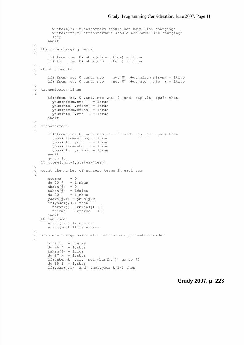
7/22/2019 Fundamentals Grady Notes June 2007 Print
http://slidepdf.com/reader/full/fundamentals-grady-notes-june-2007-print 223/388
Grady, Programming Consideration, June 2007, Page 11
write(6,*) 'transformers should not have line charging'write(iout,*) 'transformers should not have line charging'stop
endifcc the line charging termsc
if(nfrom .ne. 0) ybus(nfrom,nfrom) = ltrueif(nto .ne. 0) ybus(nto ,nto ) = ltrue
cc shunt elementsc if(nfrom .ne. 0 .and. nto .eq. 0) ybus(nfrom,nfrom) = ltrue
if(nfrom .eq. 0 .and. nto .ne. 0) ybus(nto ,nto ) = ltruecc transmission linesc if(nfrom .ne. 0 .and. nto .ne. 0 .and. tap .lt. eps6) then
ybus(nfrom,nto ) = ltrueybus(nto ,nfrom) = ltrueybus(nfrom,nfrom) = ltrue
ybus(nto ,nto ) = ltrueendifcc transformersc if(nfrom .ne. 0 .and. nto .ne. 0 .and. tap .ge. eps6) then
ybus(nfrom,nfrom) = ltrueybus(nto ,nto ) = ltrueybus(nfrom,nto ) = ltrueybus(nto ,nfrom) = ltrue
endifgo to 10
15 close(unit=1,status='keep')c
c count the number of nonzero terms in each rowc nterms = 0
do 20 j = 1,nbusnbran(j) = 0taken(j) = lfalsedo 20 k = 1,nbusysave(j,k) = ybus(j,k)if(ybus(j,k)) thennbran(j) = nbran(j) + 1nterms = nterms + 1
endif 20 continue write(6,1111) nterms
write(iout,1111) ntermscc simulate the gaussian elimination using file=bdat orderc ntfill = nterms
do 96 j = 1,nbustaken(j) = ltruedo 97 k = 1,nbusif(taken(k) .or. .not.ybus(k,j)) go to 97do 98 l = 1,nbusif(ybus(j,l) .and. .not.ybus(k,l)) then
Grady 2007, p. 223
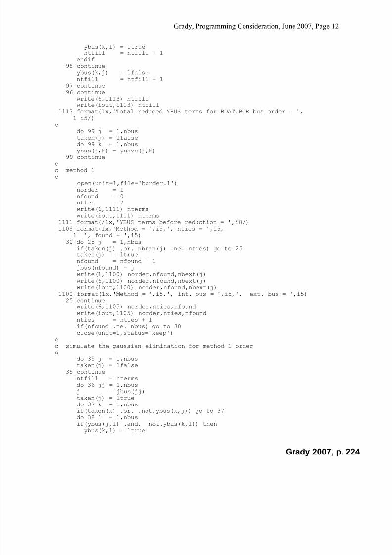
7/22/2019 Fundamentals Grady Notes June 2007 Print
http://slidepdf.com/reader/full/fundamentals-grady-notes-june-2007-print 224/388
Grady, Programming Consideration, June 2007, Page 12
ybus(k,l) = ltruentfill = ntfill + 1
endif98 continue
ybus(k,j) = lfalsentfill = ntfill - 1
97 continue
96 continue write(6,1113) ntfill
write(iout,1113) ntfill1113 format(1x,'Total reduced YBUS terms for BDAT.BOR bus order = ',
1 i5/)c do 99 j = 1,nbus
taken(j) = lfalsedo 99 k = 1,nbusybus(j,k) = ysave(j,k)
99 continuecc method 1c
open(unit=1,file='border.1')norder = 1nfound = 0nties = 2write(6,1111) ntermswrite(iout,1111) nterms
1111 format(/1x,'YBUS terms before reduction = ',i8/)1105 format(1x,'Method = ',i5,', nties = ',i5,
1 ', found = ',i5)30 do 25 j = 1,nbus
if(taken(j) .or. nbran(j) .ne. nties) go to 25taken(j) = ltruenfound = nfound + 1jbus(nfound) = j
write(1,1100) norder,nfound,nbext(j)write(6,1100) norder,nfound,nbext(j)write(iout,1100) norder,nfound,nbext(j)
1100 format(1x,'Method = ',i5,', int. bus = ',i5,', ext. bus = ',i5) 25 continue
write(6,1105) norder,nties,nfoundwrite(iout,1105) norder,nties,nfoundnties = nties + 1if(nfound .ne. nbus) go to 30close(unit=1,status='keep')
cc simulate the gaussian elimination for method 1 orderc do 35 j = 1,nbus
taken(j) = lfalse35 continue
ntfill = ntermsdo 36 jj = 1,nbusj = jbus(jj)taken(j) = ltruedo 37 k = 1,nbusif(taken(k) .or. .not.ybus(k,j)) go to 37do 38 l = 1,nbusif(ybus(j,l) .and. .not.ybus(k,l)) then
ybus(k,l) = ltrue
Grady 2007, p. 224

7/22/2019 Fundamentals Grady Notes June 2007 Print
http://slidepdf.com/reader/full/fundamentals-grady-notes-june-2007-print 225/388
Grady, Programming Consideration, June 2007, Page 13
ntfill = ntfill + 1endif
38 continueybus(k,j) = lfalsentfill = ntfill - 1
37 continue36 continue
write(6,1122) norder,ntfillwrite(iout,1122) norder,ntfill
1122 format(/1x,'Total reduced YBUS terms for method = ',i5,1' equals ',i5/)
cc method 2c open(unit=1,file='border.2')
norder = 2do 40 j = 1,nbusnbran(j) = 0taken(j) = lfalsedo 40 k = 1,nbusybus(j,k) = ysave(j,k)
if(ybus(j,k)) nbran(j) = nbran(j) + 140 continuenfound = 0ntfill = nterms
nties = 2write(6,1111) ntermswrite(iout,1111) nterms
1108 format(1x,'Method = ',i5,', nties = ',i5,1 ', found = ',i5,', tot. terms = ',i5)
50 do 45 j = 1,nbusif(taken(j) .or. nbran(j) .ne. nties) go to 45taken(j) = ltruenfound = nfound + 1write(1,1100) norder,nfound,nbext(j)
write(6,1100) norder,nfound,nbext(j)write(iout,1100) norder,nfound,nbext(j)cc gaussian eliminate all the remaining rows with row jc do 60 k = 1,nbus
if(k .eq. j .or. taken(k)) go to 60if(ybus(k,j)) thendo 65 l = 1,nbusif(l .eq. j) go to 65if(ybus(j,l) .and. .not.ybus(k,l)) thenybus(k,l) = ltruenbran(k) = nbran(k) + 1ntfill = ntfill + 1
endif65 continue
cc for the term under the pivotc ybus(k,j) = lfalse
nbran(k) = nbran(k) - 1ntfill = ntfill - 1
endif 60 continue
write(6,1108) norder,nties,nfound,ntfill
Grady 2007, p. 225

7/22/2019 Fundamentals Grady Notes June 2007 Print
http://slidepdf.com/reader/full/fundamentals-grady-notes-june-2007-print 226/388
Grady, Programming Consideration, June 2007, Page 14
write(iout,1108) norder,nties,nfound,ntfillif(nfound .eq. nbus) go to 59nties = 2if(nfound .eq. (nbus - 1)) nties = 1go to 50
45 continuenties = nties + 1
go to 5059 close(unit=1,status='keep')
write(6,1122) norder,ntfillwrite(iout,1122) norder,ntfill
cc method 3c open(unit=1,file='border.3')
norder = 3do 160 j = 1,nbustaken(j) = lfalsedo 160 k = 1,nbusybus(j,k) = ysave(j,k)
160 continue
nfound = 0nfills = 0ntfill = ntermswrite(6,1111) ntermswrite(iout,1111) nterms
170 write(6,1107) norder,nfills,nfound,ntfillwrite(iout,1107) norder,nfills,nfound,ntfill
1107 format(1x,'Method = ',i5,', nfills = ',i5,1 ', found = ',i5,', tot. terms = ',i5)
cc simulated gaussian elimination using the remaining pivot candidatesc mfirst = 0
nxtbus = 0
do 165 m = 1,nbusif(taken(m)) go to 165lstbus = mnfills = 0do 180 k = 1,nbusif(k .eq. m .or. taken(k)) go to 180if(ybus(k,m)) thendo 185 l = 1,nbusif(l .eq. m) go to 185if(ybus(m,l) .and. .not.ybus(k,l)) nfills = nfills + 1
185 continuecc for the term under the pivotc nfills = nfills - 1
endif 180 continue
if(mfirst .eq. 0) thenmfirst = 1nxtbus = mminfil = nfills
endifif(nfills .lt. minfil) thennxtbus = mminfil = nfills
Grady 2007, p. 226
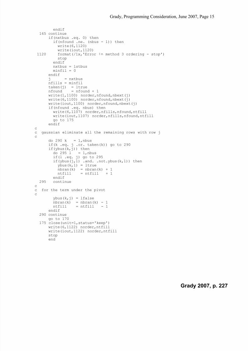
7/22/2019 Fundamentals Grady Notes June 2007 Print
http://slidepdf.com/reader/full/fundamentals-grady-notes-june-2007-print 227/388
Grady, Programming Consideration, June 2007, Page 15
endif 165 continue
if(nxtbus .eq. 0) thenif(nfound .ne. (nbus - 1)) thenwrite(6,1120)write(iout,1120)
1120 format(/1x,'Error in method 3 ordering - stop')
stopendifnxtbus = lstbusminfil = 0
endif j = nxtbus
nfills = minfiltaken(j) = ltruenfound = nfound + 1write(1,1100) norder,nfound,nbext(j)write(6,1100) norder,nfound,nbext(j)write(iout,1100) norder,nfound,nbext(j)if(nfound .eq. nbus) thenwrite(6,1107) norder,nfills,nfound,ntfill
write(iout,1107) norder,nfills,nfound,ntfillgo to 175endif
cc gaussian eliminate all the remaining rows with row jc do 290 k = 1,nbus
if(k .eq. j .or. taken(k)) go to 290if(ybus(k,j)) thendo 295 l = 1,nbusif(l .eq. j) go to 295if(ybus(j,l) .and. .not.ybus(k,l)) thenybus(k,l) = ltruenbran(k) = nbran(k) + 1
ntfill = ntfill + 1endif295 continue
cc for the term under the pivotc ybus(k,j) = lfalse
nbran(k) = nbran(k) - 1ntfill = ntfill - 1
endif 290 continue
go to 170175 close(unit=1,status='keep')
write(6,1122) norder,ntfillwrite(iout,1122) norder,ntfillstopend
Grady 2007, p. 227

7/22/2019 Fundamentals Grady Notes June 2007 Print
http://slidepdf.com/reader/full/fundamentals-grady-notes-june-2007-print 228/388
Grady, Motor Starting, June 2007, Page 1
Motor Starting
Steady-state analysis of the motor starting problem.
1. Characteristics of Motors During Start-Up
During start-up, motors behave like fixed impedances that, at rated voltage, draw approximately
five-times their full-load running current, and at a very low power factor. If the motor terminal
voltage drops to less than 80% during start-up, most motors will not start.
2. Determination of Motor Start-Up Voltage
The equivalent circuit for calculating motor starting voltages is shown in Figure 1.
Zm
Zth
Vm+
-
Vth+
-
Figure 1. Motor Starting Equivalent Circuit
This Thevenin equivalent circuit has open-circuit voltage V TH = 1.0 pu, and Thevenin
impedance Z TH , which is the "short circuit," positive-sequence impedance of the system as
"seen" at the motor terminals. Z TH
is the motor-bus diagonal element of the positive-sequence
impedance matrix, which is computed with all other large machines represented by their
respective subtransient impedances.
The motor is represented at start-up as fixed impedance Z R jX M M M , where R X M M and
are calculated to give approximately five-times full-load running current @ 1.0 pu voltage, and
at a startup-up power factor of approximately 0.20.
Given the circuit parameters, the motor start-up voltage is then computed from the voltage
divider equation, or
V V Z
Z Z M TH M
TH M .
V M should not be less than 0.80 pu. if the motor is start properly.
This problem can be worked "in reverse," where the objective is to determine how large a motor
will start at a bus. A FORTRAN code for this purpose is shown below.
c
Grady 2007, p. 228

7/22/2019 Fundamentals Grady Notes June 2007 Print
http://slidepdf.com/reader/full/fundamentals-grady-notes-june-2007-print 229/388
Grady, Motor Starting, June 2007, Page 2
c program motors.f reads zbus1 and vsoln files, and then computesc the kw motor that can be started at each bus without dragging thec voltage below vmin (in percent). the results are written to filec mstart.c complex zzz,zmotor
character*12 anames,an
dimension anames(9999),hpmin(9999)data anames /9999 * ' '/, hpmin /9999 * -1.0/
cc abase = base current,c vbase = base voltage - volts (three-phase),c pbase = base power - va (three-phase),c arun = running amps per kw,c spf = motor power factor when starting,c rpf = motor power factor when running,c start = multiplier of run current when starting,c vmin = minimum acceptable starting voltage - pu.c data pbase/100000.0/,vbase/450.0/,spf/0.2/,start/5.0/
data vmin/0.8/,rpf/0.85/eps/1.0e-03/
c abase = pbase / 3.0 / vbase * sqrt(3.0)arun = 1000.0 / 3.0 / rpf / vbase * sqrt(3.0)write(6,5007) abase,arun
5007 format(1x,'base current = ',f10.2/1x,'running current ',1'for 1 kw = ',f10.2)
cc zmotor = motor starting impedance for a 1 kw motorc zmotor = abase / arun / start *
1 cmplx(spf,sqrt(1.0 - spf * spf))write(6,5006) zmotor
5006 format(1x,'z start for a 1 kw motor = ',2e15.6)rm = real(zmotor)
xm = aimag(zmotor)open(unit=1,file='vsoln')open(unit=2,file='zbus1')open(unit=3,file='mstart')
1 read(1,5000,end=2) kbus,an5000 format(1x,i4,2x,a12)
if(kbus .le. 0 .or. kbus .gt. 9999) go to 500anames(kbus) = ango to 1
2 read(2,5002,end=3) jbus,kbus,zzz5002 format(1x,2i5,2e15.6)
if(jbus .ne. kbus) go to 2rs = real(zzz)xs = aimag(zzz)a = (vmin * vmin - 1) * (rm * rm + xm * xm)b = 2.0 * vmin * vmin * (rs * rm + xs * xm)c = vmin * vmin * (rs * rs + xs * xs)rad = sqrt(b * b - 4.0 * a * c)h1 = 1.0 / ((-b + rad) / 2.0 / a)h2 = 1.0 / ((-b - rad) / 2.0 / a)h = -1.0if(h1 .lt. 0.0 .and. h2 .gt. 0.0) h = h2if(h2 .lt. 0.0 .and. h1 .gt. 0.0) h = h1if(h1 .gt. 0.0 .and. h2 .gt. 0.0) h = amin1(h1,h2)if(h .le. 0.0) go to 501
Grady 2007, p. 229
7/22/2019 Fundamentals Grady Notes June 2007 Print
http://slidepdf.com/reader/full/fundamentals-grady-notes-june-2007-print 230/388
Grady, Motor Starting, June 2007, Page 3
if(hpmin(jbus) .lt. 0.0) hpmin(jbus) = hif(h .lt. hpmin(jbus)) hpmin(jbus) = hwrite(6,5003) jbus,anames(jbus),zzz,h
5003 format(1x,'num = ',i4,', name = ',a12,', zsys = ',2e12.4,1 ', kw = ',f7.1)vcheck = cabs(zmotor / h / (zzz + zmotor / h))if(vcheck .lt. (vmin - eps) .or. vcheck .gt. (vmin + eps))
1 go to 502go to 2
3 do 5 jbus = 1,9999if(hpmin(jbus) .lt. 0.0) go to 5write(3,5011) jbus,anames(jbus),hpmin(jbus)
5011 format(1x,'bus number = ',i5,', name = ',a12,1', kw starting cap. = ',f7.1)5 continuestop
500 write(6,5001)5001 format(1x,'error in vsoln file')
stop501 write(6,5005)
5005 format(1x,'error in kw calculation')
stop502 write(6,5010)5010 format(1x,'error in vcheck')
stopend
Grady 2007, p. 230

7/22/2019 Fundamentals Grady Notes June 2007 Print
http://slidepdf.com/reader/full/fundamentals-grady-notes-june-2007-print 231/388
Grady 2007, p. 231
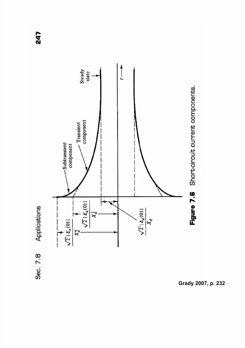
7/22/2019 Fundamentals Grady Notes June 2007 Print
http://slidepdf.com/reader/full/fundamentals-grady-notes-june-2007-print 232/388
Grady 2007, p. 232

7/22/2019 Fundamentals Grady Notes June 2007 Print
http://slidepdf.com/reader/full/fundamentals-grady-notes-june-2007-print 233/388
B e r g e n , C h a p t e r 1 2 , p . 4 6 8
Grady 2007, p. 233
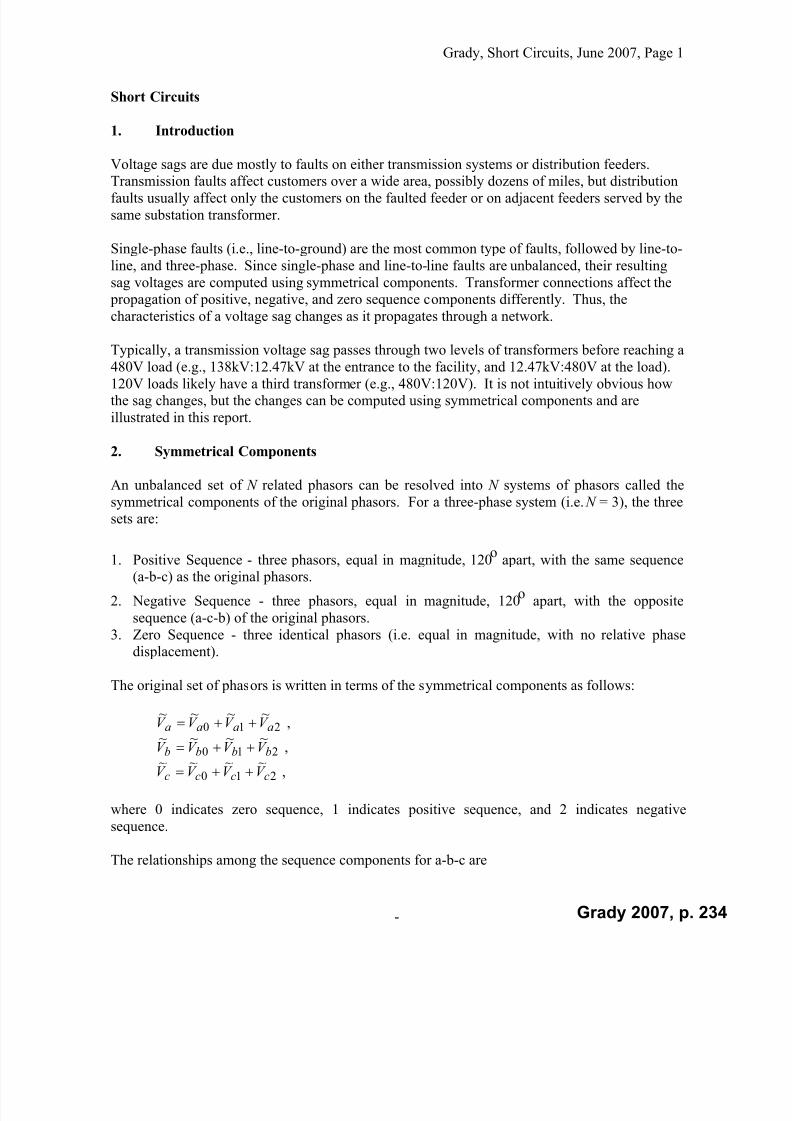
7/22/2019 Fundamentals Grady Notes June 2007 Print
http://slidepdf.com/reader/full/fundamentals-grady-notes-june-2007-print 234/388
Grady, Short Circuits, June 2007, Page 1
-
Short Circuits
1. Introduction
Voltage sags are due mostly to faults on either transmission systems or distribution feeders.
Transmission faults affect customers over a wide area, possibly dozens of miles, but distributionfaults usually affect only the customers on the faulted feeder or on adjacent feeders served by the
same substation transformer.
Single-phase faults (i.e., line-to-ground) are the most common type of faults, followed by line-to-
line, and three-phase. Since single-phase and line-to-line faults are unbalanced, their resulting
sag voltages are computed using symmetrical components. Transformer connections affect the propagation of positive, negative, and zero sequence components differently. Thus, the
characteristics of a voltage sag changes as it propagates through a network.
Typically, a transmission voltage sag passes through two levels of transformers before reaching a
480V load (e.g., 138kV:12.47kV at the entrance to the facility, and 12.47kV:480V at the load).120V loads likely have a third transformer (e.g., 480V:120V). It is not intuitively obvious howthe sag changes, but the changes can be computed using symmetrical components and are
illustrated in this report.
2. Symmetrical Components
An unbalanced set of N related phasors can be resolved into N systems of phasors called the
symmetrical components of the original phasors. For a three-phase system (i.e. N = 3), the threesets are:
1. Positive Sequence - three phasors, equal in magnitude, 120o apart, with the same sequence
(a-b-c) as the original phasors.
2. Negative Sequence - three phasors, equal in magnitude, 120o apart, with the opposite
sequence (a-c-b) of the original phasors.
3. Zero Sequence - three identical phasors (i.e. equal in magnitude, with no relative phasedisplacement).
The original set of phasors is written in terms of the symmetrical components as follows:
210~~~~aaaa V V V V ,
210~~~~bbbb V V V V ,
210~~~~cccc V V V V ,
where 0 indicates zero sequence, 1 indicates positive sequence, and 2 indicates negative
sequence.
The relationships among the sequence components for a-b-c are
Grady 2007, p. 234
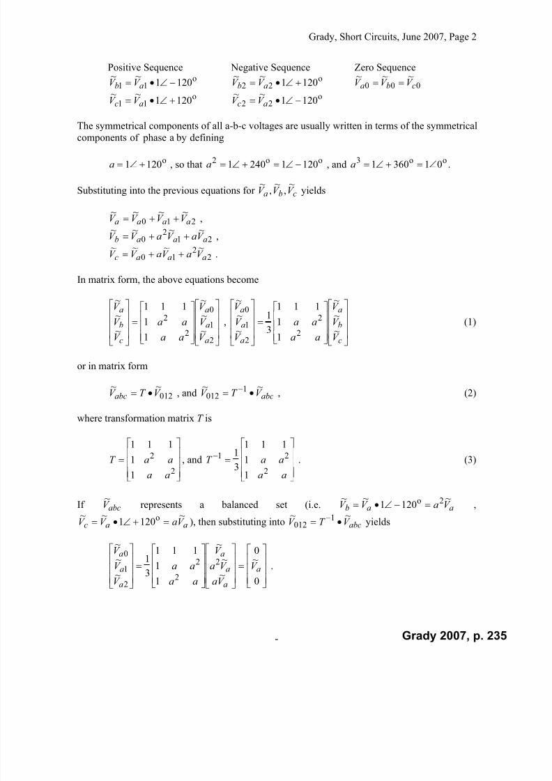
7/22/2019 Fundamentals Grady Notes June 2007 Print
http://slidepdf.com/reader/full/fundamentals-grady-notes-june-2007-print 235/388
Grady, Short Circuits, June 2007, Page 2
-
Positive Sequence Negative Sequence Zero Sequence~ ~V V b a1 1 1 120o ~ ~
V V b a2 2 1 120o000
~~~cba V V V
~ ~V V c a1 1 1 120o ~ ~
V V c a2 2 1 120o
The symmetrical components of all a-b-c voltages are usually written in terms of the symmetricalcomponents of phase a by defining
a 1 120o , so that a2 1 1 240 120o o , and a3 1 1 360 0o o .
Substituting into the previous equations for~
,~
,~
V V V a b c yields
~ ~ ~ ~V V V V a a a a 0 1 2 ,
212
0~~~~aaab V aV aV V ,
~ ~ ~ ~V V aV a V
c a a a
0 1
2
2 .
In matrix form, the above equations become
2
1
0
2
2
~
~
~
1
1
111
~
~
~
a
a
a
c
b
a
V
V
V
aa
aa
V
V
V
,
c
b
a
a
a
a
V
V
V
aa
aa
V
V
V
~
~
~
1
1
111
3
1
~
~
~
2
2
2
1
0
(1)
or in matrix form
~ ~V T V abc 012 , and ~ ~V T V abc012 1 , (2)
where transformation matrix T is
T a a
a a
1 1 1
1
1
2
2
, and T a a
a a
1 2
2
1
3
1 1 1
1
1
. (3)
If ~V abc represents a balanced set (i.e.
~ ~ ~V V a V b a a 1 2120o ,
~ ~ ~V V aV c a a 1 120o ), then substituting into ~ ~V T V abc012 1 yields
~
~
~
~
~
~
~V
V
V
a a
a a
V
a V
aV
V
a
a
a
a
a
a
a
0
1
2
2
2
21
3
1 1 1
1
1
0
0
.
Grady 2007, p. 235

7/22/2019 Fundamentals Grady Notes June 2007 Print
http://slidepdf.com/reader/full/fundamentals-grady-notes-june-2007-print 236/388
Grady, Short Circuits, June 2007, Page 3
-
Hence, balanced voltages or currents have only positive sequence components, and the positive
sequence components equal the corresponding phase a voltages or currents.
However, balanced voltages are rare during voltage sags. Most often, one phase is affected
significantly, and the other two less significantly. Thus, all three sequence voltages
210
~,
~,
~aaa V V V exist during most sags, and these sequence voltages are shifted differently by
transformers when propagating through a system. When recombined to yield phase voltages
cba V V V ~
,~
,~
, it is clear that the form of phase voltages must also change as transformers are
encountered.
3. Transformer Phase Shift
The conventional positive-sequence and negative-sequence model for a three-phase transformer
is shown below. Admittance y is a series equivalent for resistance and leakage reactance, tap t is
the tap (in per unit), and angle is the phase shift.
y
Ii ---> Ik --->Bus i
Bus k t / :1
Bus k'
Figure 1. Positive- and Negative-Sequence Model of Three-Phase Transformer
For grounded-wye:grounded-wye and delta:delta transformers, is +0˚, and thus positive- and
negative-sequence voltages and currents pass through unaltered (in per unit). However, for wye-delta and delta-wye transformers, is sequence-dependent and is defined as follows:
For positive sequence, is +30˚ if bus i is the high-voltage side, or –30˚ if bus i is thelow-voltage side
and oppositely
For negative sequence, is –30˚ if bus i is the high-voltage side, or +30˚ if bus i is the
low-voltage side
In other words, positive sequence voltages and currents on the high-voltage side lead those onthe low-voltage side by 30˚. Negative sequence voltages and currents on the high-voltage side
lag those on the low-voltage side by 30˚.
For zero-sequence voltages and currents, transformers do not introduce a phase shift, but they
may block zero-sequence propagation as shown in Figure 2.
Grady 2007, p. 236
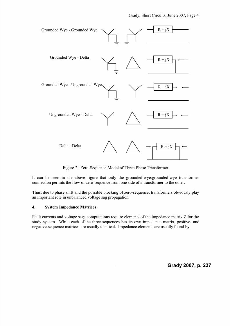
7/22/2019 Fundamentals Grady Notes June 2007 Print
http://slidepdf.com/reader/full/fundamentals-grady-notes-june-2007-print 237/388
Grady, Short Circuits, June 2007, Page 4
-
Grounded Wye - Grounded Wye
Grounded Wye - DeltaR + jX
Grounded Wye - Ungrounded WyeR + jX
R + jXUngrounded Wye - Delta
R + jXDelta - Delta
R + jX
Figure 2. Zero-Sequence Model of Three-Phase Transformer
It can be seen in the above figure that only the grounded-wye:grounded-wye transformer
connection permits the flow of zero-sequence from one side of a transformer to the other.
Thus, due to phase shift and the possible blocking of zero-sequence, transformers obviously playan important role in unbalanced voltage sag propagation.
4. System Impedance Matrices
Fault currents and voltage sags computations require elements of the impedance matrix Z for thestudy system. While each of the three sequences has its own impedance matrix, positive- andnegative-sequence matrices are usually identical. Impedance elements are usually found by
Grady 2007, p. 237
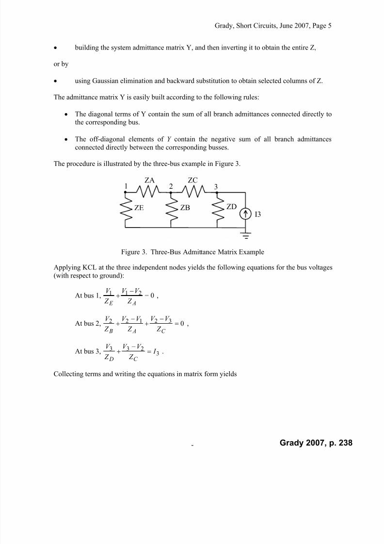
7/22/2019 Fundamentals Grady Notes June 2007 Print
http://slidepdf.com/reader/full/fundamentals-grady-notes-june-2007-print 238/388
Grady, Short Circuits, June 2007, Page 5
-
building the system admittance matrix Y, and then inverting it to obtain the entire Z,
or by
using Gaussian elimination and backward substitution to obtain selected columns of Z.
The admittance matrix Y is easily built according to the following rules:
The diagonal terms of Y contain the sum of all branch admittances connected directly tothe corresponding bus.
The off-diagonal elements of Y contain the negative sum of all branch admittances
connected directly between the corresponding busses.
The procedure is illustrated by the three-bus example in Figure 3.
1 2 3
ZE
ZA
ZB
ZC
ZDI3
Figure 3. Three-Bus Admittance Matrix Example
Applying KCL at the three independent nodes yields the following equations for the bus voltages(with respect to ground):
At bus 1, 0211
A E Z
V V
Z
V ,
At bus 2, 032122
C A B Z
V V
Z
V V
Z
V ,
At bus 3, 3233 I
Z
V V
Z
V
C D
.
Collecting terms and writing the equations in matrix form yields
Grady 2007, p. 238

7/22/2019 Fundamentals Grady Notes June 2007 Print
http://slidepdf.com/reader/full/fundamentals-grady-notes-june-2007-print 239/388
Grady, Short Circuits, June 2007, Page 6
-
33
2
1
0
0
1110
11111
0111
I V
V
V
Z Z Z
Z Z Z Z Z
Z Z Z
DC C
C C B A A
A A E
,
or in matrix form,
I YV ,
Besides being the key for fault calculations, the impedance matrix, 1 Y Z , is also physically
significant. Consider Figure 4.
Power System
All Other Busses
Open Circuited
Applied Current at
Induced Voltage
+
-
V
Bus k at Bus j
Ik
Vj
Figure 4. Physical Significance of the Impedance Matrix
Impedance matrix element k j z , is defined as
k m N mm I k
jk j
I
V z
,,,2,1,0
,
, (4)
where k I is a current source attached to bus k , jV is the resulting voltage at bus j, and all busses
except k are open-circuited. The depth of a voltage sag at bus k is determined directly bymultiplying the phase sequence components of the fault current at bus k by the matrix elements
k j z , for the corresponding phase sequences.
5. Short Circuit Calculations
Short circuit calculations require positive, negative, and zero sequence impedance information,
depending on whether or the fault is balanced or not. For example, the commonly-studied, but
relatively rare, three-phase fault is balanced. Therefore, only positive sequence impedances arerequired for its study.
Grady 2007, p. 239

7/22/2019 Fundamentals Grady Notes June 2007 Print
http://slidepdf.com/reader/full/fundamentals-grady-notes-june-2007-print 240/388
Grady, Short Circuits, June 2007, Page 7
-
Consider the three-phase fault represented by the one-line diagram in Figure 5, where TH V and
TH Z are the Thevenin equivalent circuit parameters for bus k.
+
-
Vth
Zth
ZFIF
Bus k
Figure 5. Three-Phase Fault at Bus k
The fault current and voltage are clearly
F TH
TH F k Z Z
V I
, and
F TH
F TH
F k TH TH
F k Z Z
Z V I Z V V .
In a large power system, the Thevenin equivalent impedance for a bus is the corresponding
diagonal impedance matrix element, and the Thevenin equivalent voltage is usually assumed to
be 1.0 /0 pu.
The type of machine models used when building impedance matrices affects the Thevenin
equivalent impedances and fault calculations. Rotating machines actually have time-varyingimpedances when subjected to disturbances. However, for simplification purposes, their
impedances are usually divided into three zones - subtransient (first few cycles), transient (5
cycles - 60 cycles), and steady-state (longer than 60 cycles). When performing fault studies, the
time period of interest is usually a few cycles, so that machines are represented by theirsubtransient impedances when forming the impedance matrices.
Developing the equations for fault studies requires adept use of both a-b-c and 0-1-2 forms of thecircuit equations. The use of sequence components implies that the system impedances (but not
the system voltages and currents) are symmetric. In general, there are six equations and sixunknowns to be solved, regardless of the type of fault studied.
It is common in fault studies to assume that the power system is initially unloaded and that allvoltages are 1.0 per unit. When there are multiple sources, this assumption requires that there
are no shunt elements connected, such as loads, capacitors, etc., except for rotating machines
(whose Thevenin equivalent voltages are 1.0 pu.).
Since wye-delta transformers shift positive, negative, and zero sequence components differently,
it is important to model transformers according to the rules given earlier. This means that the pre-fault voltages all have magnitude 1.0 pu., but that the pre-fault voltage angles can be
ooo 30or ,30,0 , depending upon the net transformer phase shift between them and the chosen
reference bus.
Grady 2007, p. 240

7/22/2019 Fundamentals Grady Notes June 2007 Print
http://slidepdf.com/reader/full/fundamentals-grady-notes-june-2007-print 241/388
Grady, Short Circuits, June 2007, Page 8
-
Balanced Three-Phase Fault
Consider the three-phase fault at bus k , as shown in Figure 6.
a
b
c
ZF ZF ZF
IkaF
IkcF
IkbF
Bus k
Figure 6: Three-Phase Fault at Bus k
The Thevenin equivalent circuit equation, assuming no other current injections in the system, is
F kc
F kb
F ka
kckckbkckakc
kckbkbkbkakb
kckakbkakaka
ekc
ekb
eka
F kc
F kb
F ka
I
I
I
z z z
z z z
z z z
V
V
V
V
V
V
,,,
,,,
,,,
Pr
Pr
Pr
,
or in sequence form,
F k
F k
F k
k k
k k
k k
ek
ek
ek
F k
F k
F k
I
I
I
z
z
z
V
V
V
V
V
V
2
1
0
2,2
1,1
0,0
Pr 2
Pr 1
Pr 0
2
1
0
00
00
00
.
In abbreviated form, the above equations are
F kabcabck k
ekabc
F kabc
I Z V V ,Pr
, and F k k k
ek
F k
I Z V V 012012,
Pr 012012 , (5)
where F k
V consists of the voltages at bus k during the fault, ek
V Pr consists of the pre-fault
voltages, F k
I gives the fault currents, and k k Z contains the individual impedance elements
extracted from the impedance matrix.
Grady 2007, p. 241

7/22/2019 Fundamentals Grady Notes June 2007 Print
http://slidepdf.com/reader/full/fundamentals-grady-notes-june-2007-print 242/388
Grady, Short Circuits, June 2007, Page 9
-
The above matrix equations represents three equations (repeated in abc and 012 form), but there
are six unknowns represented by F k
V and F k
I , so that three additional equations are required.
The additional equations are found by observing that
F
kabc F
F
kabc I Z V , or
F
k F
F
k I Z V 012012 .
Substituting into the Thevenin equation, and recognizing that all zero- and negative-sequence
voltages and currents are zero for a balanced fault yields
0
0
00
00
00
0
0
0
0
1
2,2
1,1
0,0Pr 11
F k
k k
k k
k k e
k F k F I
z
z
z
V I Z ,
so that the positive sequence fault current is found to be
0,0,20
1,1
Pr 1
1
F
k F k
F k k
ek F
k I I
Z z
V I . (6)
Substituting into Thevenin equation
F k k k
ek
F k
I Z V V 012012,
Pr 012012 (7)
yields the fault voltage at Bus k . Similarly, because the impedance matrix relates the voltages at
network busses to current injections at network busses, the voltage at any other bus j is foundusing
F k k j
e j
F j I Z V V
012012,Pr 012012 . (8)
Note that the minus sign is needed because the fault current has been drawn as positive outward.
Once the fault voltages are known at neighboring busses, the contribution currents through theconnected branches can be easily found.
Single-Phase to Ground Fault
Consider the single-phase fault at bus k , as shown in Figure 7.
Grady 2007, p. 242

7/22/2019 Fundamentals Grady Notes June 2007 Print
http://slidepdf.com/reader/full/fundamentals-grady-notes-june-2007-print 243/388
Grady, Short Circuits, June 2007, Page 10
-
a
b
c
ZF
IkaF
Bus k
Ikb
F = 0
IkcF = 0
Figure 7: Single-Phase Fault at Bus k , Phase a
As before, the Thevenin equivalent circuit equations, assuming no other current injections in the
system, is
F k k k
ek
F k
I Z V V 012012,
Pr 012012 .
Examining F k
I 012
shows that in this case
F ka
F ka
F ka
F kc
F kb
F ka
F kabc
F k
I
I
I
I
I
I
aa
aa I T I 31
0
0
1
1
111
31
2
21012 . (9)
Substituting into the Thevenin equation yields
3/
3/
3/
00
00
00
0
0
2,2
1,1
0,0
Pr 2
Pr Pr 1
Pr 0
2
1
0
F ka
F ka
F ka
k k
k k
k k
ek
eka
ek
ek
F k
F k
F k
I
I
I
z
z
z
V
V V
V
V
V
V
Add the three rows yields
2,21,10,0Pr
210 3
1k k k k k k
F ka
eka
F ka
F k
F k
F k
z z z I V V V V V .
From the circuit it is obvious that
Grady 2007, p. 243

7/22/2019 Fundamentals Grady Notes June 2007 Print
http://slidepdf.com/reader/full/fundamentals-grady-notes-june-2007-print 244/388
Grady, Short Circuits, June 2007, Page 11
-
F F ka
F ka
Z I V ,
so that
2,21,10,0Pr
3
1k k k k k k
F ka
eka F
F ka z z z I V Z I .
Solving for F ka
I yields
F k k k k k k
eka F
ka Z z z z
V I
3
3
2,21,10,0
Pr
. (10)
Now, using
3210
F
ka F k
F k
F k I I I I ,
all network voltages can be found from
F k k j
e j
F j I Z V V
012012,Pr 012012 .
Note that if 2,10,0 k k k k z z , a single-phase fault will have a higher value than does a three-
phase fault.
Line-to-Line Fault
Consider the line-to-line fault at bus k , as shown in Figure 8.
a
b
c
IkcF
Bus k
IkaF = 0
ZF
IkbF
Figure 8. Line-to-Line Fault Between Phases b and c at Bus k
Examining F k
I 012
shows that in this case
Grady 2007, p. 244

7/22/2019 Fundamentals Grady Notes June 2007 Print
http://slidepdf.com/reader/full/fundamentals-grady-notes-june-2007-print 245/388
Grady, Short Circuits, June 2007, Page 12
-
aa I
aa I
I I
I
I
aa
aa I T I
F kb
F kb
F kb
F kc
F kb
F ka
F kabc
F k
2
2
2
21012
0
3
10
1
1
111
3
1 . (11)
Note that there is no zero sequence fault current.
Substituting into the Thevenin equation yields
3/
3/
0
00
00
00
0
0
2
2
2,2
1,1
0,0Pr
2
1
0
aa I
aa I
z
z
z
V
V
V
V
F kb
F kb
k k
k k
k k e
ka F k
F k
F k
.
Subtracting the last two rows of the Thevenin equation yields
33
2
2,2
2
1,1Pr
21
aa I z
aa I z V V V
F kb
k k
F kb
k k e
ka F k
F k
,
or
eka
F k
F k
k k k k F kb
V V V aa z aa z
I Pr 21
21,1
22,2
33
.
From the circuit, we see that
F
F kc
F kb F
kb Z
V V I
.
Using 012TV V abc , we find that
22
21
aaV aaV V V F k
F k
F kc
F kb
,
so that
F
F k
F k F
kb F
F k
F k F
kb Z
aaV V I
Z
aaV aaV I
221
22
21 or , .
Combining equations yields
Grady 2007, p. 245

7/22/2019 Fundamentals Grady Notes June 2007 Print
http://slidepdf.com/reader/full/fundamentals-grady-notes-june-2007-print 246/388
Grady, Short Circuits, June 2007, Page 13
-
eka
F F kbk k k k F
kb V
aa
Z I aa z aa z I Pr
2
21,1
22,2
33
.
Collecting terms yields
eka
F k k k k F kb
V aa
Z aa z aa z I Pr
2
21,1
22,2
33
,
or
ekak k k k
F F kb
V z z aa
aa
Z I Pr
2,21,1
2
2 3
.
Simplifying yields
and where 0, F ka
F kb
F kc
I I I . All network voltages can now be found from
F k k k k
eka F
kb Z z z
V j I
2,21,1
Pr 3 , (12)
F k k j
e j
F j I Z V V 012012,
Pr 012012 .
Grady 2007, p. 246
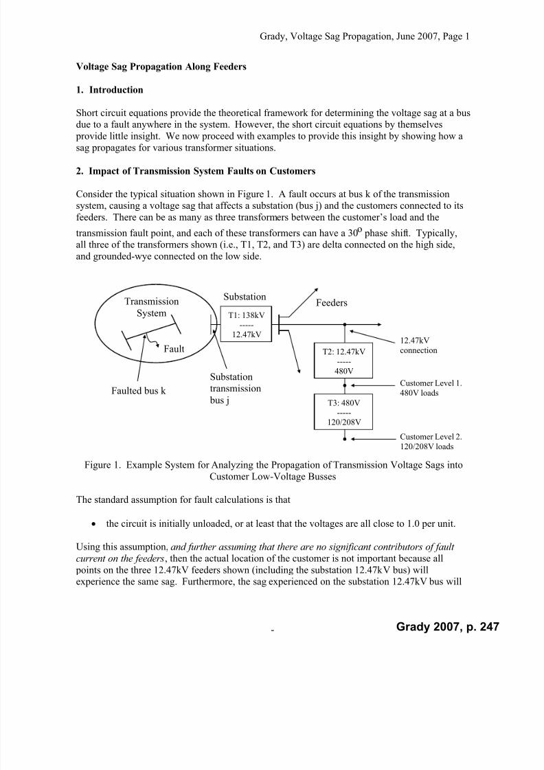
7/22/2019 Fundamentals Grady Notes June 2007 Print
http://slidepdf.com/reader/full/fundamentals-grady-notes-june-2007-print 247/388
Grady, Voltage Sag Propagation, June 2007, Page 1
-
Voltage Sag Propagation Along Feeders
1. Introduction
Short circuit equations provide the theoretical framework for determining the voltage sag at a bus
due to a fault anywhere in the system. However, the short circuit equations by themselves provide little insight. We now proceed with examples to provide this insight by showing how a
sag propagates for various transformer situations.
2. Impact of Transmission System Faults on Customers
Consider the typical situation shown in Figure 1. A fault occurs at bus k of the transmissionsystem, causing a voltage sag that affects a substation (bus j) and the customers connected to its
feeders. There can be as many as three transformers between the customer’s load and the
transmission fault point, and each of these transformers can have a 30o phase shift. Typically,all three of the transformers shown (i.e., T1, T2, and T3) are delta connected on the high side,
and grounded-wye connected on the low side.
Figure 1. Example System for Analyzing the Propagation of Transmission Voltage Sags into
Customer Low-Voltage Busses
The standard assumption for fault calculations is that
the circuit is initially unloaded, or at least that the voltages are all close to 1.0 per unit.
Using this assumption, and further assuming that there are no significant contributors of faultcurrent on the feeders, then the actual location of the customer is not important because all
points on the three 12.47kV feeders shown (including the substation 12.47kV bus) willexperience the same sag. Furthermore, the sag experienced on the substation 12.47kV bus will
Transmission
System
T2: 12.47kV
-----
480V
T3: 480V
-----120/208V
T1: 138kV-----
12.47kV
SubstationFeeders
Customer Level 1.480V loads
Customer Level 2.
120/208V loads
12.47kV
connectionFault
Substation
transmission bus j
Faulted bus k
Grady 2007, p. 247

7/22/2019 Fundamentals Grady Notes June 2007 Print
http://slidepdf.com/reader/full/fundamentals-grady-notes-june-2007-print 248/388
Grady, Voltage Sag Propagation, June 2007, Page 2
-
be the same as on substation 138kV bus j, except for possible zero-sequence component blocking
and positive/negative-phase shifts.
The significance of the above paragraph is that
for transmission faults, one monitor at either the substation 138kV bus or at the substation12.47kV bus is adequate to predict voltage sag levels anywhere on the substation’s feeders, provided there are no significant contributors of fault current on the feeders.
If the transmission fault is electrically far away, then the sag experienced at the substation and at
the customer site will be small. Alternatively, if the fault is immediately at substation 138kV bus
j, then the sag will be the most severe possible. Thus, it is reasonable to assume that an electrical“proximity” factor exists, where a proximity factor of zero (i.e., 0%) indicates that the fault is at
substation 138kV bus j, and a proximity factor of unity (i.e., 100%) indicates that the
transmission fault bus k is very far away. From knowledge of the physical significance of theimpedance matrix, and from examining Thevenin equations
F k k k
ek
F k
I Z V V 012012,
Pr 012012 ,
F k k j
e j
F j I Z V V
012012,Pr 012012 ,
this proximity factor P is approximated using the ratio of positive-sequence impedances
1,1
1,11
k k
k j
z
z P . (1)
By coding the short circuit equations into a Visual Basic program, and employing (1), voltage
sag propagation for the situation described in Figure 1 can now be illustrated. Assuming that thetransmission fault is relatively close to the substation (i.e., proximity factor = 25%), and that T1,
T2, and T3 are all delta:grounded-wye transformers, the line-to-neutral voltages for single-phase,
phase-to-phase, and three-phase transmission faults are shown in Figures 2 – 4, respectively.
Both phasor plots and magnitude bar charts are given.
It is important to note that if a transformer is connected grounded-wye:grounded-wye or
delta:delta, then the voltage sag on the low-voltage side of the transformer is the same as on thehigh-voltage side, as illustrated in Figure 5 for the single-phase fault.
Grady 2007, p. 248
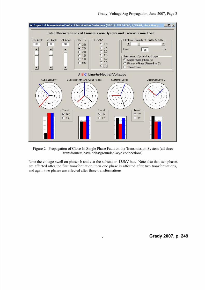
7/22/2019 Fundamentals Grady Notes June 2007 Print
http://slidepdf.com/reader/full/fundamentals-grady-notes-june-2007-print 249/388
Grady, Voltage Sag Propagation, June 2007, Page 3
-
Figure 2. Propagation of Close-In Single Phase Fault on the Transmission System (all three
transformers have delta:grounded-wye connections)
Note the voltage swell on phases b and c at the substation 138kV bus. Note also that two phases
are affected after the first transformation, then one phase is affected after two transformations,and again two phases are affected after three transformations.
Grady 2007, p. 249

7/22/2019 Fundamentals Grady Notes June 2007 Print
http://slidepdf.com/reader/full/fundamentals-grady-notes-june-2007-print 250/388
Grady, Voltage Sag Propagation, June 2007, Page 4
-
Figure 3. Propagation of Close-In Phase-to-Phase Fault on the Transmission System (all three
transformers have delta:grounded-wye connections)
Grady 2007, p. 250

7/22/2019 Fundamentals Grady Notes June 2007 Print
http://slidepdf.com/reader/full/fundamentals-grady-notes-june-2007-print 251/388
Grady, Voltage Sag Propagation, June 2007, Page 5
-
Figure 4. Propagation of Close-In Three-Phase Fault on the Transmission System (all three
transformers have delta:grounded-wye connections)
Grady 2007, p. 251

7/22/2019 Fundamentals Grady Notes June 2007 Print
http://slidepdf.com/reader/full/fundamentals-grady-notes-june-2007-print 252/388
Grady, Voltage Sag Propagation, June 2007, Page 6
-
Figure 5. Situation in Figure 2 Repeated, but with all Three Transformers Having Grounded-
Wye:Grounded-Wye Connections
Grady 2007, p. 252

7/22/2019 Fundamentals Grady Notes June 2007 Print
http://slidepdf.com/reader/full/fundamentals-grady-notes-june-2007-print 253/388
Grady, Voltage Sag Propagation, June 2007, Page 7
-
3. Impact of Distribution System Faults on Adjacent Feeders
Now, consider the situation in Figure 6 where a fault occurs on an adjacent feeder, and a monitor
records the voltage waveform at the substation 12.47kV bus.
Figure 6. Substation Monitor Records Voltages when a Sag Occurs on an Adjacent Feeder.
As in Section 2, unless the customer’s feeder has significant contributors to the fault current, the
voltage sag at the substation 12.47kV bus will appear everywhere along the customer’s 12.47kVfeeder. However, to predict the voltage sag at Customer Levels 1 and 2, the a-b-c line-to-neutral
voltages at the substation 12.47kV bus must be
converted to positive/negative/zero-sequence components,
shifted with the appropriate transformer phase shifts,
converted back to a-b-c.
Ideally, the monitor should report phasor voltage magnitudes and angles during the sag
condition, rather than time-sampled data points for which phase angles must be estimated.
The conversion/shifting/re-conversion procedure has been coded into a Visual Basic program
and is illustrated in Figure 7 to illustrate the propagation of a sag due to a single-phase faultthrough two levels of delta:grounded-wye transformers inside a customer’s facility. Thesubstation 12.47kV voltage entered is approximately the same as predicted in Figure 2.
T2: 12.47kV
-----
480V
T3: 480V
-----120/208V
T1: 138kV
-----
12.47kV
Substation
Customer Level 1.
480V loads
Customer Level 2.
120/208V loads
12.47kV
connection
138kV
Fault on adjacent
feeder
Monitor observes
voltage waveform
Grady 2007, p. 253

7/22/2019 Fundamentals Grady Notes June 2007 Print
http://slidepdf.com/reader/full/fundamentals-grady-notes-june-2007-print 254/388
Grady, Voltage Sag Propagation, June 2007, Page 8
-
Figure 7. Propagation of Voltage Sag Due to Single-Phase Fault on Adjacent Feeder
Each vertical column in Figure 7 indicates the following voltages: 1. on the feeder, 2. after one
level of delta:grounded-wye transformer, and 3. after a second level of delta:grounded-wye
transformer. The four vertical columns correspond to various locations down the feeder, provided that sequence impedances of the feeder are entered. For Figure 7, all four columns are
identical since no feeder currents and feeder impedances were entered.
4. Impact of Distribution System Faults on the Customer’s Feeder
To analyze voltage sags on a faulted feeder, feeder currents must be known. Consider thesituation in Figure 8. The Thevenin-equivalent impedance at Customer 1 is Z1, followed by
incremental impedances dZ between the other customers that are distributed down the feeder.
Grady 2007, p. 254
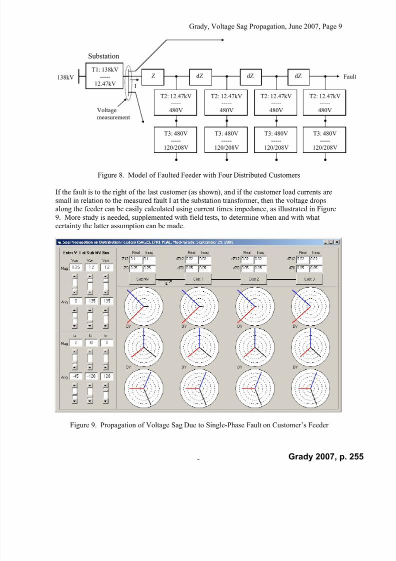
7/22/2019 Fundamentals Grady Notes June 2007 Print
http://slidepdf.com/reader/full/fundamentals-grady-notes-june-2007-print 255/388
Grady, Voltage Sag Propagation, June 2007, Page 9
-
Figure 8. Model of Faulted Feeder with Four Distributed Customers
If the fault is to the right of the last customer (as shown), and if the customer load currents aresmall in relation to the measured fault I at the substation transformer, then the voltage drops
along the feeder can be easily calculated using current times impedance, as illustrated in Figure
9. More study is needed, supplemented with field tests, to determine when and with what
certainty the latter assumption can be made.
Figure 9. Propagation of Voltage Sag Due to Single-Phase Fault on Customer’s Feeder
T2: 12.47kV
-----
480V
T3: 480V
-----
120/208V
T1: 138kV
-----
12.47kV
Substation
138kV Fault
T2: 12.47kV
-----
480V
T3: 480V
-----
120/208V
T2: 12.47kV
-----
480V
T3: 480V
-----
120/208V
T2: 12.47kV
-----
480V
T3: 480V
-----
120/208V
Z dZ dZdZ
I
Voltage
measurement
Grady 2007, p. 255

7/22/2019 Fundamentals Grady Notes June 2007 Print
http://slidepdf.com/reader/full/fundamentals-grady-notes-june-2007-print 256/388

7/22/2019 Fundamentals Grady Notes June 2007 Print
http://slidepdf.com/reader/full/fundamentals-grady-notes-june-2007-print 257/388
The positive-sequence one-line diagram for a network is shown below. The ground ties
at busses 1 and 4 represent the subtransient impedances of machines. Prefault voltagesare all 1.0pu.
a. Use the definition
k mm I k
j
k
j jk I
V I V z
,0
to fill in column 1 of the Z matrix.
Now, a solidly-grounded three-phase fault occurs at bus 1.
b. Compute the fault currentc. Use the fault current and Z matrix terms to compute the voltages at busses 2 and 3.
d. Find the magnitude of the current flowing in the line connecting busses 2 and 3.
1 2 3
1
2
3
j0.2
j0.3
j0.1
j0.05
Bus 1
Bus 2
Bus 3
j0.1
+
1/0
–
+1/0
–
Grady 2007, p. 257

7/22/2019 Fundamentals Grady Notes June 2007 Print
http://slidepdf.com/reader/full/fundamentals-grady-notes-june-2007-print 258/388
Grady 2007, p. 258
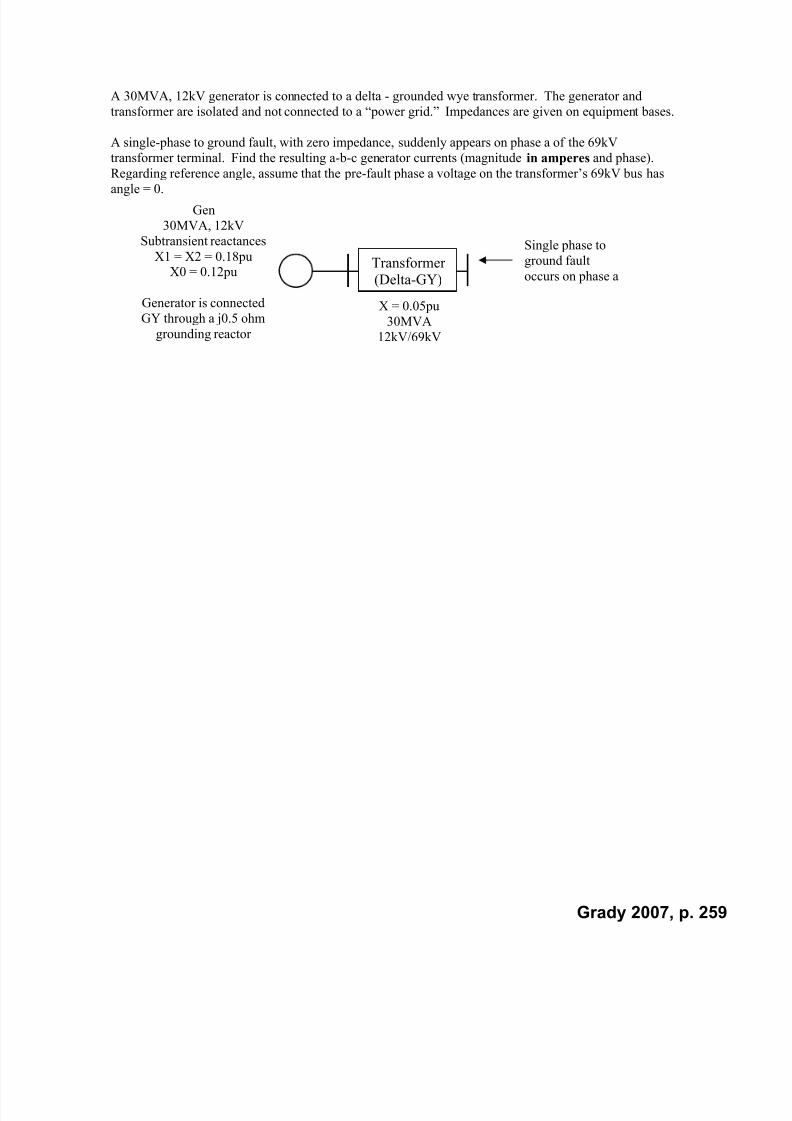
7/22/2019 Fundamentals Grady Notes June 2007 Print
http://slidepdf.com/reader/full/fundamentals-grady-notes-june-2007-print 259/388
A 30MVA, 12kV generator is connected to a delta - grounded wye transformer. The generator and
transformer are isolated and not connected to a “power grid.” Impedances are given on equipment bases.
A single-phase to ground fault, with zero impedance, suddenly appears on phase a of the 69kV
transformer terminal. Find the resulting a-b-c generator currents (magnitude in amperes and phase).
Regarding reference angle, assume that the pre-fault phase a voltage on the transformer’s 69kV bus has
angle = 0.
Gen
30MVA, 12kV
Subtransient reactances
X1 = X2 = 0.18puX0 = 0.12pu
Generator is connected
GY through a j0.5 ohm
grounding reactor
X = 0.05pu
30MVA
12kV/69kV
Single phase to
ground fault
occurs on phase aTransformer(Delta-GY)
Grady 2007, p. 259
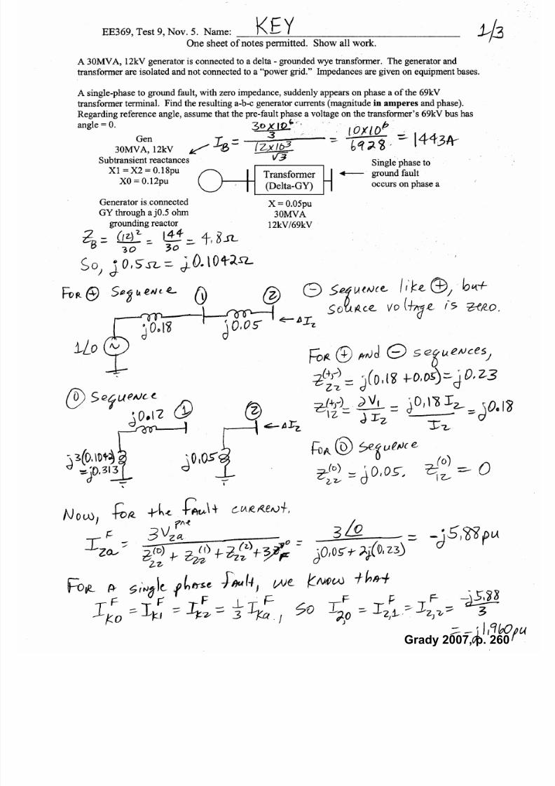
7/22/2019 Fundamentals Grady Notes June 2007 Print
http://slidepdf.com/reader/full/fundamentals-grady-notes-june-2007-print 260/388
Grady 2007, p. 260

7/22/2019 Fundamentals Grady Notes June 2007 Print
http://slidepdf.com/reader/full/fundamentals-grady-notes-june-2007-print 261/388
Grady 2007, p. 261

7/22/2019 Fundamentals Grady Notes June 2007 Print
http://slidepdf.com/reader/full/fundamentals-grady-notes-june-2007-print 262/388
Grady 2007, p. 262
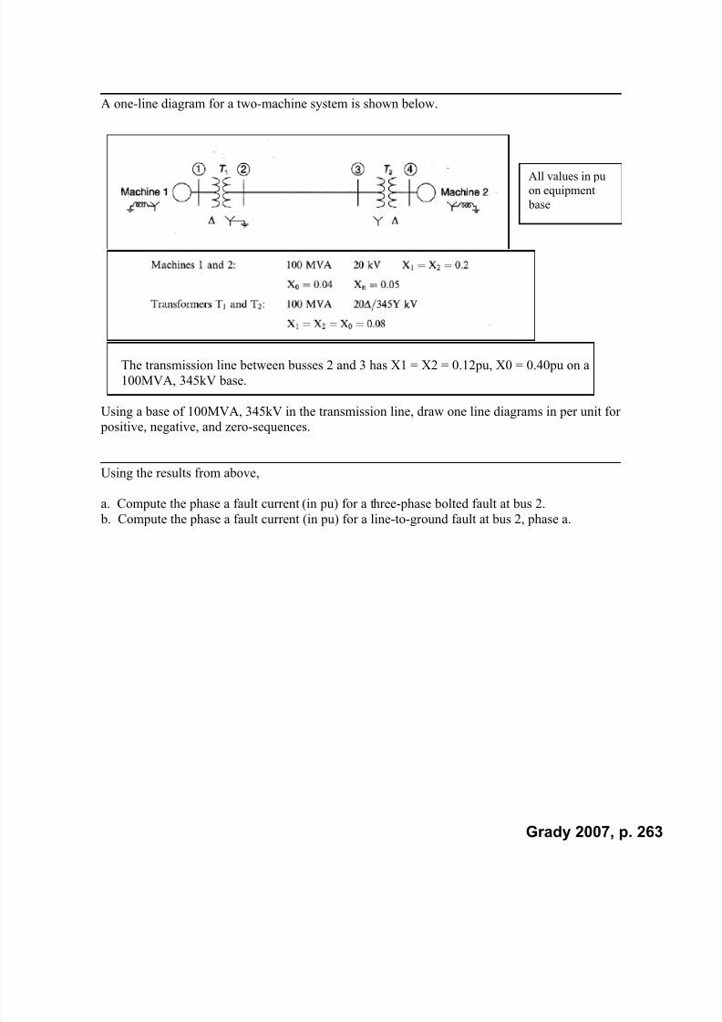
7/22/2019 Fundamentals Grady Notes June 2007 Print
http://slidepdf.com/reader/full/fundamentals-grady-notes-june-2007-print 263/388
A one-line diagram for a two-machine system is shown below.
The transmission line between busses 2 and 3 has X1 = X2 = 0.12pu, X0 = 0.40pu on a
100MVA, 345kV base.
Using a base of 100MVA, 345kV in the transmission line, draw one line diagrams in per unit for positive, negative, and zero-sequences.
Using the results from above,
a. Compute the phase a fault current (in pu) for a three-phase bolted fault at bus 2.
b. Compute the phase a fault current (in pu) for a line-to-ground fault at bus 2, phase a.
All values in pu
on equipment
base
Grady 2007, p. 263

7/22/2019 Fundamentals Grady Notes June 2007 Print
http://slidepdf.com/reader/full/fundamentals-grady-notes-june-2007-print 264/388
Grady 2007, p. 264

7/22/2019 Fundamentals Grady Notes June 2007 Print
http://slidepdf.com/reader/full/fundamentals-grady-notes-june-2007-print 265/388
Stevenson Six-Bus Short Circuit Example. Fault at Bus 4.
Grady 2007, p. 265
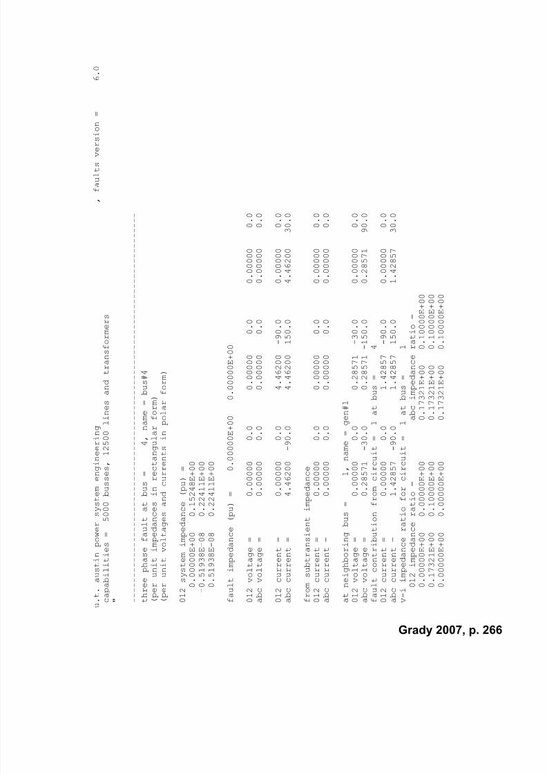
7/22/2019 Fundamentals Grady Notes June 2007 Print
http://slidepdf.com/reader/full/fundamentals-grady-notes-june-2007-print 266/388
u . t . a u s t i n p o w e r s
y s t e m e n g i n e e r i n g
,
f a u l t s v e r s i o
n =
6 . 0
c a p a b i l i t i e s =
5 0
0 0
b u s s e s ,
1 2 5 0 0
l i n e s a n
d t r a n s f o r m e r s
" - - - - - - - - - - - - - - - - - -
- - - - - - - - - - - - - - - - - - - - - - - - -
- - - - - - - - - - - - - - - - - - - - - - - - - -
- - - - - - - -
t h r e e p h a s e
f a u l t
a t
b u s =
4 , n a m e =
b u
s # 4
( p e r u n i t
i m p e d a n c
e s
i n r e c t a n g u l a r
f o r m )
( p e r u n i t v o l t a g e s
a n d c u r r e n t s
i n p o l a r
f o
r m )
0 1 2 s y s t e m
i m p e d a n
c e
( p u ) =
0 . 0 0 0 0 0 E + 0 0
0
. 1 5 2 4 8 E + 0 0
- 0 . 5 1 9 3 8 E - 0 8
0
. 2 2 4 1 1 E + 0 0
0 . 5 1 9 3 8 E - 0 8
0
. 2 2 4 1 1 E + 0 0
f a u l t
i m p e d a n c e
( p
u ) =
0 . 0 0 0 0 0 E + 0 0
0 . 0
0 0 0 0 E + 0 0
0 1 2 v o l t a g e =
0 . 0 0 0 0 0
0 . 0
0
. 0 0 0 0 0
0 . 0
0 . 0 0 0 0
0
0 . 0
a b c v o l t a g e =
0 . 0 0 0 0 0
0 . 0
0
. 0 0 0 0 0
0 . 0
0 . 0 0 0 0
0
0 . 0
0 1 2 c u r r e n t =
0 . 0 0 0 0 0
0 . 0
4
. 4 6 2 0 0
- 9 0 . 0
0 . 0 0 0 0
0
0 . 0
a b c c u r r e n t =
4 . 4 6 2 0 0
- 9 0 . 0
4
. 4 6 2 0 0
1 5 0 . 0
4 . 4 6 2 0
0
3 0 . 0
f r o m s u b t r a n s i e n t
i m p e d a n c e
0 1 2 c u r r e n t =
0 . 0 0 0 0 0
0 . 0
0
. 0 0 0 0 0
0 . 0
0 . 0 0 0 0
0
0 . 0
a b c c u r r e n t =
0 . 0 0 0 0 0
0 . 0
0
. 0 0 0 0 0
0 . 0
0 . 0 0 0 0
0
0 . 0
a t n e i g h b o r i n g
b u s
=
1 , n a m e = g e n # 1
0 1 2 v o l t a g e =
0 . 0 0 0 0 0
0 . 0
0
. 2 8 5 7 1
- 3 0 . 0
0 . 0 0 0 0
0
0 . 0
a b c v o l t a g e =
0 . 2 8 5 7 1
- 3 0 . 0
0
. 2 8 5 7 1 - 1 5 0 . 0
0 . 2 8 5 7
1
9 0 . 0
f a u l t c o n t r i b u t i o n
f r o m c i r c u i t =
1 a t
b u s
=
4
0 1 2 c u r r e n t =
0 . 0 0 0 0 0
0 . 0
1
. 4 2 8 5 7
- 9 0 . 0
0 . 0 0 0 0
0
0 . 0
a b c c u r r e n t =
1 . 4 2 8 5 7
- 9 0 . 0
1
. 4 2 8 5 7
1 5 0 . 0
1 . 4 2 8 5
7
3 0 . 0
v - i
i m p e d a n c e r a t i
o
f o r c i r c u i t =
1 a t
b u s
=
1
0 1 2
i m p e d a n c e r
a t i o =
a b c
i m p
e d a n c e r a t i o =
0 . 0 0 0 0 0 E + 0 0
0
. 0 0 0 0 0 E + 0 0
0 . 1 7 3 2 1
E + 0 0
0 . 1 0 0 0 0 E + 0 0
0 . 1 7 3 2 1 E + 0 0
0
. 1 0 0 0 0 E + 0 0
0 . 1 7 3 2 1
E + 0 0
0 . 1 0 0 0 0 E + 0 0
0 . 0 0 0 0 0 E + 0 0
0
. 0 0 0 0 0 E + 0 0
0 . 1 7 3 2 1
E + 0 0
0 . 1 0 0 0 0 E + 0 0
Grady 2007, p. 266

7/22/2019 Fundamentals Grady Notes June 2007 Print
http://slidepdf.com/reader/full/fundamentals-grady-notes-june-2007-print 267/388
a t n e i g h b o r i n g
b u s
=
5 , n a m e =
b u s # 5
0 1 2 v o l t a g e =
0 . 0 0 0 0 0
0 . 0
0
. 2 5 0 5 6
0 . 0
0 . 0 0 0 0
0
0 . 0
a b c v o l t a g e =
0 . 2 5 0 5 6
0 . 0
0
. 2 5 0 5 6 - 1 2 0 . 0
0 . 2 5 0 5
6
1 2 0 . 0
f a u l t c o n t r i b u t i o n
f r o m c i r c u i t =
1 a t
b u s
=
4
0 1 2 c u r r e n t =
0 . 0 0 0 0 0
0 . 0
3
. 0 3 3 4 3
- 9 0 . 0
0 . 0 0 0 0
0
0 . 0
a b c c u r r e n t =
3 . 0 3 3 4 3
- 9 0 . 0
3
. 0 3 3 4 3
1 5 0 . 0
3 . 0 3 3 4
3
3 0 . 0
v - i
i m p e d a n c e r a t i
o
f o r c i r c u i t =
1 a t
b u s
=
5
0 1 2
i m p e d a n c e r
a t i o =
a b c
i m p
e d a n c e r a t i o =
0 . 0 0 0 0 0 E + 0 0
0
. 0 0 0 0 0 E + 0 0
- 0 . 2 1 3 8 6
E - 1 5
0 . 8 2 6 0 0 E - 0 1
0 . 5 1 2 4 1 E - 0 8
0
. 8 2 6 0 0 E - 0 1
0 . 6 5 0 2 1
E - 0 8
0 . 8 2 6 0 0 E - 0 1
0 . 0 0 0 0 0 E + 0 0
0
. 0 0 0 0 0 E + 0 0
0 . 8 8 7 0 2
E - 0 8
0 . 8 2 6 0 0 E - 0 1
e n d o f t h r e e p h a s e
f a u l t r e p o r t
- - - - - - - - - - - - - - - - - -
- - - - - - - - - - - - - - - - - - - - - - - - -
- - - - - - - - - - - - - - - - - - - - - - - - - -
- - - - - - - -
l i n e - t o - l i n e
f a u l t
a t
b u s =
4 , n a m e =
b
u s # 4
( p e r u n i t
i m p e d a n c
e s
i n r e c t a n g u l a r
f o r m )
( p e r u n i t v o l t a g e s
a n d c u r r e n t s
i n p o l a r
f o
r m )
0 1 2 s y s t e m
i m p e d a n
c e
( p u ) =
0 . 0 0 0 0 0 E + 0 0
0
. 1 5 2 4 8 E + 0 0
- 0 . 5 1 9 3 8 E - 0 8
0
. 2 2 4 1 1 E + 0 0
0 . 5 1 9 3 8 E - 0 8
0
. 2 2 4 1 1 E + 0 0
f a u l t
i m p e d a n c e
( p
u ) =
0 . 0 0 0 0 0 E + 0 0
0 . 0
0 0 0 0 E + 0 0
0 1 2 v o l t a g e =
0 . 0 0 0 0 0
0 . 0
0
. 5 0 0 0 0
0 . 0
0 . 5 0 0 0
0
0 . 0
a b c v o l t a g e =
1 . 0 0 0 0 0
0 . 0
0
. 5 0 0 0 0 - 1 8 0 . 0
0 . 5 0 0 0
0
1 8 0 . 0
0 1 2 c u r r e n t =
0 . 0 0 0 0 0
0 . 0
2
. 2 3 1 0 0
- 9 0 . 0
2 . 2 3 1 0
0
9 0 . 0
a b c c u r r e n t =
0 . 0 0 0 0 0
0 . 0
3
. 8 6 4 2 1
1 8 0 . 0
3 . 8 6 4 2
1
0 . 0
f r o m s u b t r a n s i e n t
i m p e d a n c e
0 1 2 c u r r e n t =
0 . 0 0 0 0 0
0 . 0
0
. 0 0 0 0 0
0 . 0
0 . 0 0 0 0
0
0 . 0
a b c c u r r e n t =
0 . 0 0 0 0 0
0 . 0
0
. 0 0 0 0 0
0 . 0
0 . 0 0 0 0
0
0 . 0
a t n e i g h b o r i n g
b u s
=
1 , n a m e = g e n # 1
0 1 2 v o l t a g e =
0 . 0 0 0 0 0
0 . 0
0
. 6 4 2 8 6
- 3 0 . 0
0 . 3 5 7 1
4
3 0 . 0
Grady 2007, p. 267

7/22/2019 Fundamentals Grady Notes June 2007 Print
http://slidepdf.com/reader/full/fundamentals-grady-notes-june-2007-print 268/388
a b c v o l t a g e =
0 . 8 7 7 7 3
- 9 . 4
0
. 8 7 7 7 3 - 1 7 0 . 6
0 . 2 8 5 7
1
9 0 . 0
f a u l t c o n t r i b u t i o n
f r o m c i r c u i t =
1 a t
b u s
=
4
0 1 2 c u r r e n t =
0 . 0 0 0 0 0
0 . 0
0
. 7 1 4 2 9
- 9 0 . 0
0 . 7 1 4 2
9
9 0 . 0
a b c c u r r e n t =
0 . 0 0 0 0 0
0 . 0
1
. 2 3 7 1 8 - 1 8 0 . 0
1 . 2 3 7 1
8
0 . 0
v - i
i m p e d a n c e r a t i
o
f o r c i r c u i t =
1 a t
b u s
=
1
0 1 2
i m p e d a n c e r
a t i o =
a b c
i m p
e d a n c e r a t i o =
0 . 0 0 0 0 0 E + 0 0
0
. 0 0 0 0 0 E + 0 0
0 . 1 2 1 2 4
E + 0 1
- 0 . 2 0 0 0 0 E + 0 0
0 . 7 7 9 4 2 E + 0 0
0
. 4 5 0 0 0 E + 0 0
0 . 6 0 6 2 2
E + 0 0
0 . 1 0 0 0 0 E + 0 0
0 . 4 3 3 0 1 E + 0 0
- 0
. 2 5 0 0 0 E + 0 0
0 . 8 4 9 0 5
E - 0 7
0 . 4 0 0 0 0 E + 0 0
a t n e i g h b o r i n g
b u s
=
5 , n a m e =
b u s # 5
0 1 2 v o l t a g e =
0 . 0 0 0 0 0
0 . 0
0
. 6 2 5 2 8
0 . 0
0 . 3 7 4 7
2
0 . 0
a b c v o l t a g e =
1 . 0 0 0 0 0
0 . 0
0
. 5 4 5 0 6 - 1 5 6 . 5
0 . 5 4 5 0
6
1 5 6 . 5
f a u l t c o n t r i b u t i o n
f r o m c i r c u i t =
1 a t
b u s
=
4
0 1 2 c u r r e n t =
0 . 0 0 0 0 0
0 . 0
1
. 5 1 6 7 2
- 9 0 . 0
1 . 5 1 6 7
2
9 0 . 0
a b c c u r r e n t =
0 . 0 0 0 0 0
0 . 0
2
. 6 2 7 0 3 - 1 8 0 . 0
2 . 6 2 7 0
3
0 . 0
v - i
i m p e d a n c e r a t i
o
f o r c i r c u i t =
1 a t
b u s
=
5
0 1 2
i m p e d a n c e r
a t i o =
a b c
i m p
e d a n c e r a t i o =
0 . 0 0 0 0 0 E + 0 0
0
. 0 0 0 0 0 E + 0 0
0 . 0 0 0 0 0
E + 0 0
0 . 0 0 0 0 0 E + 0 0
0 . 2 2 5 5 2 E - 0 7
0
. 4 1 2 2 6 E + 0 0
0 . 1 9 0 3 3
E + 0 0
0 . 8 2 6 0 0 E - 0 1
- 0 . 2 9 7 5 4 E - 0 8
- 0
. 2 4 7 0 6 E + 0 0
- 0 . 1 9 0 3 3
E + 0 0
0 . 8 2 6 0 0 E - 0 1
e n d o f
l i n e - t o - l i n
e
f a u l t r e p o r t
- - - - - - - - - - - - - - - - - -
- - - - - - - - - - - - - - - - - - - - - - - - -
- - - - - - - - - - - - - - - - - - - - - - - - - -
- - - - - - - -
l i n e - t o - g r o u n d
f a u
l t a t
b u s =
4 , n a m e =
b u s # 4
( p e r u n i t
i m p e d a n c
e s
i n r e c t a n g u l a r
f o r m )
( p e r u n i t v o l t a g e s
a n d c u r r e n t s
i n p o l a r
f o
r m )
0 1 2 s y s t e m
i m p e d a n
c e
( p u ) =
0 . 0 0 0 0 0 E + 0 0
0
. 1 5 2 4 8 E + 0 0
- 0 . 5 1 9 3 8 E - 0 8
0
. 2 2 4 1 1 E + 0 0
0 . 5 1 9 3 8 E - 0 8
0
. 2 2 4 1 1 E + 0 0
f a u l t
i m p e d a n c e
( p
u ) =
0 . 0 0 0 0 0 E + 0 0
0 . 0
0 0 0 0 E + 0 0
0 1 2 v o l t a g e =
0 . 2 5 3 8 3
1 8 0 . 0
0
. 6 2 6 9 1
0 . 0
0 . 3 7 3 0
9
1 8 0 . 0
a b c v o l t a g e =
0 . 0 0 0 0 0
0 . 0
0
. 9 4 6 0 3 - 1 1 3 . 7
0 . 9 4 6 0
3
1 1 3 . 7
Grady 2007, p. 268

7/22/2019 Fundamentals Grady Notes June 2007 Print
http://slidepdf.com/reader/full/fundamentals-grady-notes-june-2007-print 269/388
0 1 2 c u r r e n t =
1 . 6 6 4 7 1
- 9 0 . 0
1
. 6 6 4 7 1
- 9 0 . 0
1 . 6 6 4 7
1
- 9 0 . 0
a b c c u r r e n t =
4 . 9 9 4 1 2
- 9 0 . 0
0
. 0 0 0 0 0
0 . 0
0 . 0 0 0 0
0
0 . 0
f r o m s u b t r a n s i e n t
i m p e d a n c e
0 1 2 c u r r e n t =
0 . 0 0 0 0 0
0 . 0
0
. 0 0 0 0 0
0 . 0
0 . 0 0 0 0
0
0 . 0
a b c c u r r e n t =
0 . 0 0 0 0 0
0 . 0
0
. 0 0 0 0 0
0 . 0
0 . 0 0 0 0
0
0 . 0
a t n e i g h b o r i n g
b u s
=
1 , n a m e = g e n # 1
0 1 2 v o l t a g e =
0 . 0 0 0 0 0
0 . 0
0
. 7 3 3 5 1
- 3 0 . 0
0 . 2 6 6 4
9 - 1 5 0 . 0
a b c v o l t a g e =
0 . 6 4 3 1 0
- 5 1 . 0
0
. 6 4 3 1 0 - 1 2 9 . 0
1 . 0 0 0 0
0
9 0 . 0
f a u l t c o n t r i b u t i o n
f r o m c i r c u i t =
1 a t
b u s
=
4
0 1 2 c u r r e n t =
1 . 2 6 9 1 5
- 9 0 . 0
0
. 5 3 2 9 8
- 9 0 . 0
0 . 5 3 2 9
8
- 9 0 . 0
a b c c u r r e n t =
2 . 3 3 5 1 1
- 9 0 . 0
0
. 7 3 6 1 7
- 9 0 . 0
0 . 7 3 6 1
7
- 9 0 . 0
v - i
i m p e d a n c e r a t i
o
f o r c i r c u i t =
1 a t
b u s
=
1
0 1 2
i m p e d a n c e r
a t i o =
a b c
i m p
e d a n c e r a t i o =
0 . 0 0 0 0 0 E + 0 0
0
. 0 0 0 0 0 E + 0 0
0 . 5 4 1 6 3
E + 0 0
0 . 4 3 8 1 2 E + 0 0
0 . 1 1 9 1 9 E + 0 1
0
. 6 8 8 1 2 E + 0 0
0 . 0 0 0 0 0
E + 0 0
0 . 0 0 0 0 0 E + 0 0
0 . 4 3 3 0 1 E + 0 0
- 0
. 2 5 0 0 0 E + 0 0
0 . 1 0 8 3 3
E + 0 1
- 0 . 3 9 6 2 0 E - 0 7
a t n e i g h b o r i n g
b u s
=
5 , n a m e =
b u s # 5
0 1 2 v o l t a g e =
0 . 1 6 7 9 9
1 8 0 . 0
0
. 7 2 0 4 0
0 . 0
0 . 2 7 9 6
0
1 8 0 . 0
a b c v o l t a g e =
0 . 2 7 2 8 0
0 . 0
0
. 9 4 9 1 3 - 1 1 4 . 2
0 . 9 4 9 1
3
1 1 4 . 2
f a u l t c o n t r i b u t i o n
f r o m c i r c u i t =
1 a t
b u s
=
4
0 1 2 c u r r e n t =
0 . 3 9 5 5 6
- 9 0 . 0
1
. 1 3 1 7 3
- 9 0 . 0
1 . 1 3 1 7
3
- 9 0 . 0
a b c c u r r e n t =
2 . 6 5 9 0 2
- 9 0 . 0
0
. 7 3 6 1 7
9 0 . 0
0 . 7 3 6 1
7
9 0 . 0
v - i
i m p e d a n c e r a t i
o
f o r c i r c u i t =
1 a t
b u s
=
5
0 1 2
i m p e d a n c e r
a t i o =
a b c
i m p
e d a n c e r a t i o =
- 0 . 4 7 3 2 0 E - 2 4
- 0
. 4 2 4 7 0 E + 0 0
0 . 1 7 0 1 8
E - 2 4
0 . 1 0 2 5 9 E + 0 0
0 . 1 5 4 7 7 E - 0 7
0
. 6 3 6 5 4 E + 0 0
- 0 . 1 1 7 6 4
E + 0 1
0 . 5 2 7 5 8 E + 0 0
- 0 . 2 9 7 5 4 E - 0 8
- 0
. 2 4 7 0 6 E + 0 0
0 . 1 1 7 6 4
E + 0 1
0 . 5 2 7 5 8 E + 0 0
e n d o f
l i n e - t o - g r o
u n d
f a u l t r e p o r t
Grady 2007, p. 269
7/22/2019 Fundamentals Grady Notes June 2007 Print
http://slidepdf.com/reader/full/fundamentals-grady-notes-june-2007-print 270/388
Grady, Loadflow, June 2007, Page 1
Loadflow
Formulation of the loadflow problem. Gauss-Seidel, Newton-Raphson, and Stott's algorithm.
Calculation of line flows, system losses, and area interchange.
1 Formulation of the Problem
The loadflow problem is one of the classic power system engineering problems. During the
early days of digital computers, many advances in techniques for solving large sets of equations
were brought about specifically to help solve the loadflow problem.
In most electrical circuit analyses, the network consists of known impedances, voltage sources,
and current sources. However, in the loadflow problem, active and reactive powers, rather than
shunt impedances, are specified at most network busses, because most loads behave, on average,
as constant power loads (active and reactive power), as long as their applied voltage remains
within reasonable ranges. Consider, for example, the air conditioning load of a building. A
certain amount of energy is required to maintain T between inside and outside temperatures.Even though the air conditioner cycles on-and-off, and the voltage may change slightly, the air
conditioning load appears, on the average, as a fixed power load, rather than as a fixed
impedance load.
Power system loads are closely monitored at substations, at large customers, and for total electric
utility companies. Loads tend to have predictable daily, weekly, and seasonal patterns. Annual
peak demands and energies for electric utilities are forecasted for generation and planning
purposes.
The purpose of the loadflow program is to compute bus voltages and line/transformer/cable
power flows once network topology, impedances, loads, and generators have been specified.Ideally, the computed bus voltages for the study system should remain within acceptable ranges,
and line/transformer/cable power flows should be below their rated values, for a reasonable set
of outage contingencies.
From a loadflow perspective, there are four parameters at every bus - voltage magnitude V ,
voltage angle , active power P , and reactive power Q. Two may be specified, and the other
two calculated. For most busses, P and Q are specified, and V and are calculated. Obviously,
P and Q cannot be specified at all busses because that would imply that system losses are known
a priori. Therefore, the loadflow problem must include one "swing bus" at which the P can
assume any value so that it "makes up" system losses. The swing bus is usually a centrally-
located large generator whose voltage magnitude and phase angle (usually = zero) arespecified.
Although any two of the four parameters can be specified, the usual way in which power system
busses are classified is given in Table 1.
Grady 2007, p. 270

7/22/2019 Fundamentals Grady Notes June 2007 Print
http://slidepdf.com/reader/full/fundamentals-grady-notes-june-2007-print 271/388
Grady, Loadflow, June 2007, Page 2
Table 1. Loadflow Classification of Power System Busses
Classification Knowns Unknowns
PQ (Load Bus) P, Q V,
PV (Generator Bus) P, V Q,
V (Swing Bus) V, P, Q
The loadflow program solves for the set of unknowns that produces power balance at all busses,
or as illustrated for bus i in Figure 1,
calci
calci
speci
speci jQ P jQ P ,
where
*ii
calci
calci I V jQ P .
In other words, the power specified at each bus must equal the power flowing into the system.
Note in Figure 1 that specified power is drawn as positive generation, to be consistent with KCL
equation YV=I .
Total Current Flowing From Bus i into the System is
P + jQi i
spec spec
IB1
IB2
IB3
Bus iBranch
Currents
Into
System
I = IB1 + IB2 + IB3i
= V Ii i*
Vi i| |
Figure 1. Power Balance for Bus i
Since there are two unknowns at every bus, the size of the loadflow problem is 2 N , where N is
the number of busses. Obviously, to solve the problem, there must be two equations for every bus. These come from KCL, which for any bus i have the form
*
1
,*
N
j j jiiii
calci
calci
speci
speci V yV I V jQ P jQ P .
Separating into real and imaginary components yields two equations for bus i,
Grady 2007, p. 271

7/22/2019 Fundamentals Grady Notes June 2007 Print
http://slidepdf.com/reader/full/fundamentals-grady-notes-june-2007-print 272/388
Grady, Loadflow, June 2007, Page 3
ji ji j ji
N
j
i speci V yV P ,,
1
cos
,
ji ji j ji
N
j i
spec
i V yV Q
,,1
sin
,
where ji ji jiiiiiii y yV V V V ,,,,, .
The problem now is now to find the set of bus voltages that satisfies the above 2 N equations.
2. Gauss-Seidel Method
Gauss-Seidel is an early formulation of the loadflow problem that requires little memory and it is
easily programmed. However, it is usually slower than other methods. It is based upon the idea
of expanding the complex form of the power balance equation as follows:
*
,1,,
*
1,
*
N
i j j j jiiiii
N
j j jiiii
speci
speci V yV yV V yV I V jQ P ,
or
N
i j j
j jiiiiii speci
speci V yV V yV jQ P
,1
,*
,* ,
so that
N
i j j
j ji
i
speci
speci
iii V y
V
jQ P
yV
,1
,*,
1 .
The solution procedure is to:
1. Initialize the bus voltages. For load busses, use V = 1 + j0. For generator busses
(including the swing bus), use 0 jV V spec .
2. One-by-one, update the individual bus voltages using
N
i j j
j ji
i
speci
speci
iii V y
V
jQ P
yV
,1
,*,
1.
For PV busses, update the voltage angle, while holding the voltage magnitude constant at
the specified value. Do not update the swing bus.
Grady 2007, p. 272
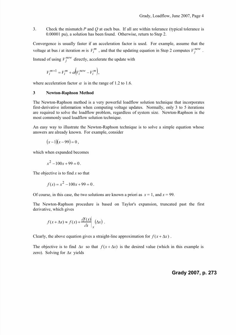
7/22/2019 Fundamentals Grady Notes June 2007 Print
http://slidepdf.com/reader/full/fundamentals-grady-notes-june-2007-print 273/388
Grady, Loadflow, June 2007, Page 4
3. Check the mismatch P and Q at each bus. If all are within tolerance (typical tolerance is
0.00001 pu), a solution has been found. Otherwise, return to Step 2.
Convergence is usually faster if an acceleration factor is used. For example, assume that the
voltage at bus i at iteration m is miV , and that the updating equation in Step 2 computes new
jV .
Instead of using new jV directly, accelerate the update with
mi
newi
mi
mi V V V V 1 ,
where acceleration factor is in the range of 1.2 to 1.6.
3 Newton-Raphson Method
The Newton-Raphson method is a very powerful loadflow solution technique that incorporates
first-derivative information when computing voltage updates. Normally, only 3 to 5 iterations
are required to solve the loadflow problem, regardless of system size. Newton-Raphson is themost commonly used loadflow solution technique.
An easy way to illustrate the Newton-Raphson technique is to solve a simple equation whose
answers are already known. For example, consider
0991 x x ,
which when expanded becomes
0991002 x x .
The objective is to find x so that
099100)( 2 x x x f .
Of course, in this case, the two solutions are known a priori as x = 1, and x = 99.
The Newton-Raphson procedure is based on Taylor's expansion, truncated past the first
derivative, which gives
x x
x f
x f x x f x
)(
)()( .
Clearly, the above equation gives a straight-line approximation for )( x x f .
The objective is to find x so that )( x x f is the desired value (which in this example is
zero). Solving for x yields
Grady 2007, p. 273

7/22/2019 Fundamentals Grady Notes June 2007 Print
http://slidepdf.com/reader/full/fundamentals-grady-notes-june-2007-print 274/388
Grady, Loadflow, June 2007, Page 5
x x
x f
x f x x f x
)(
)()( ,
which for this example is
x x x
x f
x f
x
x f
x f x
)(
)(
)(
)(0
.
The update equation for iteration (m + 1) is then
)(
)()()()1(
)(
)(
m x
mmmm
x
x f
x f x x x x
,
where in this example
1002)(
x x
x f
.
If a starting point of x = 2 is chosen, then the solution proceeds as follows:
Iteration - m x f(x) x
x f
)(
0 2 -97 -96
1 0.9896 1.0193 -98.02
2 0.9999 0.0098 -98.00
Additional iterations can be performed if tighter solution tolerance is needed. Note that if a
starting point of x = 50 had been chosen, the partial derivative would have been zero, and the
method would have failed.
If x = 80 is the starting point, then the process yields the following:
Iteration - m x f(x) x x f
)(
0 80 -1501 60
1 105.02 626.2 110.04
2 99.33 32.45 98.66
3 99.00 0 98.00
Grady 2007, p. 274
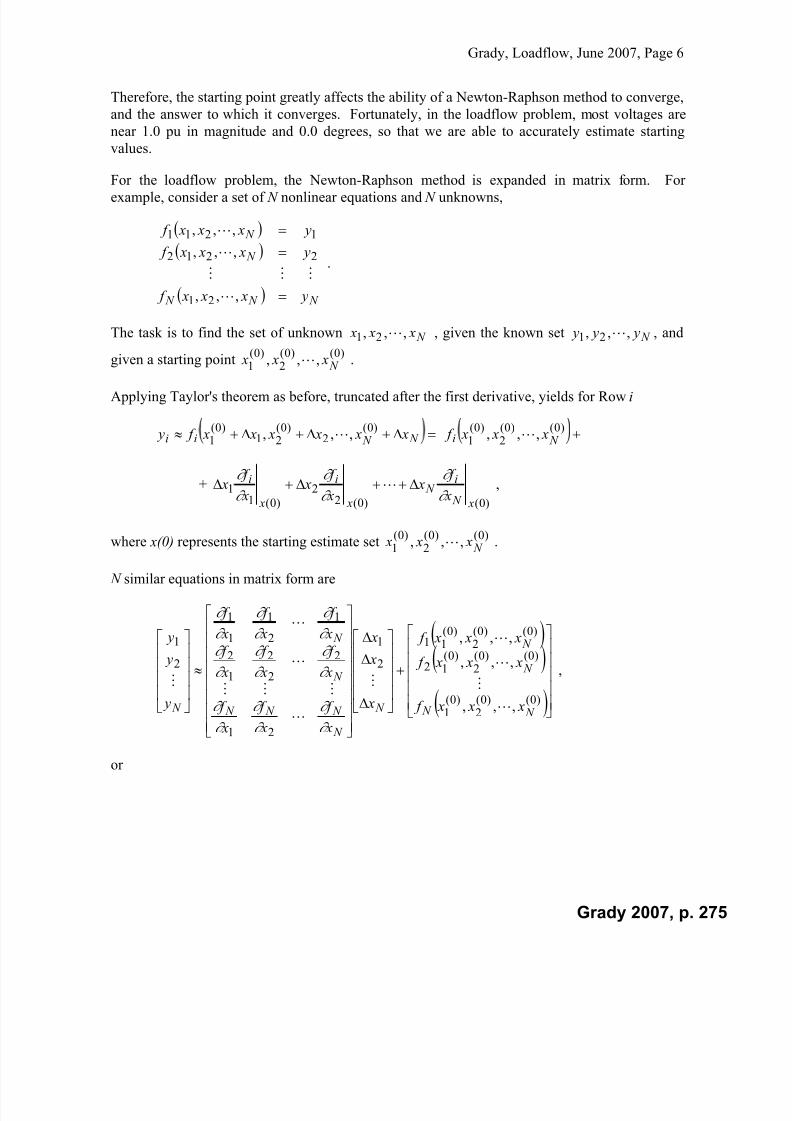
7/22/2019 Fundamentals Grady Notes June 2007 Print
http://slidepdf.com/reader/full/fundamentals-grady-notes-june-2007-print 275/388
Grady, Loadflow, June 2007, Page 6
Therefore, the starting point greatly affects the ability of a Newton-Raphson method to converge,
and the answer to which it converges. Fortunately, in the loadflow problem, most voltages are
near 1.0 pu in magnitude and 0.0 degrees, so that we are able to accurately estimate starting
values.
For the loadflow problem, the Newton-Raphson method is expanded in matrix form. Forexample, consider a set of N nonlinear equations and N unknowns,
N N N
N
N
y x x x f
y x x x f
y x x x f
,,,
,,,
,,,
21
2212
1211
.
The task is to find the set of unknown N x x x ,,, 21 , given the known set N y y y ,,, 21 , and
given a starting point)0()0(
2)0(
1 ,,, N x x x .
Applying Taylor's theorem as before, truncated after the first derivative, yields for Row i
N N ii x x x x x x f y)0(
2)0(
21)0(
1 ,,, )0()0(2
)0(1
,,, N i x x x f
+
)0()0(22
)0(11
x N
i N
x
i
x
i
x
f x
x
f x
x
f x
,
where x(0) represents the starting estimate set)0()0(
2)0(
1,,, N x x x .
N similar equations in matrix form are
)0()0(2
)0(1
)0()0(2
)0(12
)0()0(2
)0(11
2
1
21
2
2
2
1
2
1
2
1
1
1
2
1
,,,
,,,
,,,
N N
N
N
N
N
N N N
N
N
N x x x f
x x x f
x x x f
x
x
x
x
f
x
f
x
f
x
f
x
f
x
f
x
f
x
f
x
f
y
y
y
,
or
Grady 2007, p. 275

7/22/2019 Fundamentals Grady Notes June 2007 Print
http://slidepdf.com/reader/full/fundamentals-grady-notes-june-2007-print 276/388
Grady, Loadflow, June 2007, Page 7
N N N N
N
N
x
x
x
J
x x x f y
x x x f y
x x x f y
2
1
)0()0(2
)0(1
)0()0(2
)0(122
)0()0(2
)0(111
,,,
,,,
,,,
,
where J is an N x N matrix of partial derivatives, known as the Jacobian matrix. Therefore, in an
iterative procedure, the above equation is used to update the X vector according to
)(1)()()()()1( m spec
mmmmmY Y J X X X X
,
where
)()(2
)(1
)()(2
)(12
)()(2
)(11
)(2
1
,,,
,,,
,,,
,
m N
mm N
m N
mm
m N
mm
m
N
spec
x x x f
x x x f
x x x f
Y
y
y
y
Y
.
In the loadflow problem, the matrix update equation is symbolically written in mixed
rectangular-polar form as
m N
m N
mm
mm
m N
m N
mm
mm
m Ncalc Nspec
mcalc spec
mcalc spec
m Ncalc Nspec
mcalc spec
mcalc spec
V V
V V
V V V
Q J
Q J
V
P J
P J
P P
P P
P P
1
21
2
11
1
1
21
2
11
1
43
21
)(
)(22
)(11
)(
)(22
)(11
or, in abbreviated form,
V J J
J J
Q
P
43
21 .
Grady 2007, p. 276

7/22/2019 Fundamentals Grady Notes June 2007 Print
http://slidepdf.com/reader/full/fundamentals-grady-notes-june-2007-print 277/388
Grady, Loadflow, June 2007, Page 8
The dimension of the above problem is actually 2 bussesPVof Number 2 N since V
updates at PV busses are not required, and since V and updates at the swing bus are not
required.
In highly inductive power systems, P is closely related to voltage angles, and Q is closely related
to voltage magnitudes. Therefore, in the above mixed rectangular-polar formulation, the terms
in 41 and J J tend to have larger magnitudes than those in 32 and J J . This feature makes the
Jacobian matrix more diagonally dominant, which improves robustness when Gaussian
eliminating or LU decomposing J .
The above formulation of the Jacobian matrix is often modified to take advantage of symmetry
in the partial derivatives. This modification is
V
V
V QQ
V
V
P P
V
Q
P
1
1
.
The partial derivatives are derived from
ji ji j ji
N
j
icalc
i V yV P ,,
1
cos
,
ji ji j ji
N
j
icalci V yV Q ,,
1
sin
,
and have the following form
For 1 J ,
.,sin
sin
,,
,1
,,
ik V yV P
V yV P
k ik ik k ii
k
i
N
i j j
ji ji j jiii
i
For 2 J ,
Grady 2007, p. 277

7/22/2019 Fundamentals Grady Notes June 2007 Print
http://slidepdf.com/reader/full/fundamentals-grady-notes-june-2007-print 278/388
Grady, Loadflow, June 2007, Page 9
.,cos
cos2cos
,,
,,1
,,,
ik yV V
P
yV V yV
P
k ik ik iik
i
ii
N
i j j
iii ji ji j jii
i
For 3 J ,
.,cos
cos
,,
,1,,
ik V yV Q
V yV Q
k ik ik k iik
i
N
i j j
ji ji j jiii
i
For 4 J ,
.,sin
sin2sin
,,
,,1
,,,
ik yV V
Q
yV V yV
Q
k ik ik iik
i
ii
N
i j j
iii ji ji j jii
i
Note the symmetry in the J terms. If V is used as an updating parameter rather than , then
the expressions for 1 J are
.,sin
sin
,,
,1,,
ik yV V
P
V yV
P
k ik ik iik k
i
N
i j j
ji ji j jiii
i
and for 3 J ,
.,cos
cos
,,
,1,,
ik V yV
Q
V yV
Q
k ik ik k ik i
i
N
i j j
ji ji j jiii
i
and there is even more symmetry in J .
The diagonal dominance of 1 J and 4 J can be observed by the examining the partial derivatives
as follows: the differences between voltage angles at adjacent busses is usually small, so that the
Grady 2007, p. 278

7/22/2019 Fundamentals Grady Notes June 2007 Print
http://slidepdf.com/reader/full/fundamentals-grady-notes-june-2007-print 279/388
Grady, Loadflow, June 2007, Page 10
ji terms are small. The angles found in the admittance matrix are usually large (i.e. near
o90 ) because most power systems are reactive. Therefore, the sine terms in the matrix update
equation tend to be near unity, while the cosine terms tend to be near zero. Decoupled loadflow
programs use only 1 J and 4 J , treating the P and Q problems separately.
So that the benefits of optimal bus ordering can be fully exploited, non-decoupled loadflow
Jacobian matrices are usually formulated in the following alternating-row form, rather than that
described symbolically above:
N
N N
N
N
V
V
V
V
V
V
J
Q
P
Q
P
Q
P
2
22
1
11
2
2
1
1
.
The solution procedure for the Newton-Raphson loadflow proceeds with:
1. Initialize the bus voltages. For load busses, use V = 1 + j0. For generator busses
(including the swing bus), use 0 jV V spec .
2. Form the Jacobian matrix, and update all bus voltage magnitudes and phase angles,
except for those at the swing bus, and except for the voltage magnitudes at PV busses.
3. Check the mismatch P and Q at each bus. If all are within tolerance (typical tolerance is
0.00001 pu), a solution has been found. Otherwise, return to Step 2.
4 Stott's Algorithm
Stott's algorithm takes advantage of the strong decoupling of P and Q that occurs in most high-
voltage power systems. His formulation is based upon the assumption that P is primarily related
to , and that Q is primarily related to V .
He begins by writing the expression for power at bus i, which is
*
1,
N
j
j jiicalci
calci V yV jQ P .
He then defines
Grady 2007, p. 279

7/22/2019 Fundamentals Grady Notes June 2007 Print
http://slidepdf.com/reader/full/fundamentals-grady-notes-june-2007-print 280/388
Grady, Loadflow, June 2007, Page 11
ji ji ji jBG y ,,, .
Expanding the power expression yields
N
j ji ji jiii
calci
calci jBGV V jQ P
1,, ,
or, expanding in real and imaginary form
N
j
ji ji ji ji jicalc
i BGV V P
1
,,,, sincos
N
j
ji ji ji ji jicalci BGV V Q
1
,,,, cossin ,
where ji ji , .
From the above equations, the necessary loadflow partial derivatives are
ji ji ji ji ji
i j j
i BGV V P
,,,, cossin
,
and
ji ji ji ji ji
N
i j ji
i BGV V P
,,,,
,1
cossin
,
which, by comparing to the Q equation simplifies to
ii jiiiiiii
i
i BGV Q P
,,,,2
cossin
= iiii BV Q ,
2 .
Similarly, for Q,
i j
j
i
j ji ji ji jii
i j j
i P
V BGV
V
Q
1cossin ,,,, ,
and
Grady 2007, p. 280

7/22/2019 Fundamentals Grady Notes June 2007 Print
http://slidepdf.com/reader/full/fundamentals-grady-notes-june-2007-print 281/388
Grady, Loadflow, June 2007, Page 12
iiiiiiiii
N
i j j
ji ji ji ji ji
i BGV BGV V
Q,,,,
,1
,,,, cossin2cossin
.
After simplifying, the above equation becomes
iiii
i
i
i BV V
Q
V
Q,
.
The form of the Jacobian update equation is now
V
V L
H
Q
P 1
0
0 ,
where
ji BGV V L H ji ji ji ji ji ji ji ,cossin ,,,,,, ,
iiiiii BV Q H ,2
, ,
iiiiii BV Q L ,2
, .
Now, since the angular differences are small, then ji ji ,, sincos . In reactive power
systems, ji ji
G B,,
, so that ji ji ji ji
G B,,,,
sincos . Also, in most cases,
iii Q B , , so that iiii Q BV ,2 . Substituting these approximations into the above
expressions for H and L yields
ji ji ji ji BV V L H ,,, ,
iiiiiii BV L H ,2
,, .
These lead to the following simple form of the update equation:
N N N N N N
N
N
N V
V
V
B B B
B B B
B B B
V
V
V
P
2
1
2
1
,2,1,
,22,21,2
,12,11,1
2
1
00
00
00
00
00
00
Grady 2007, p. 281
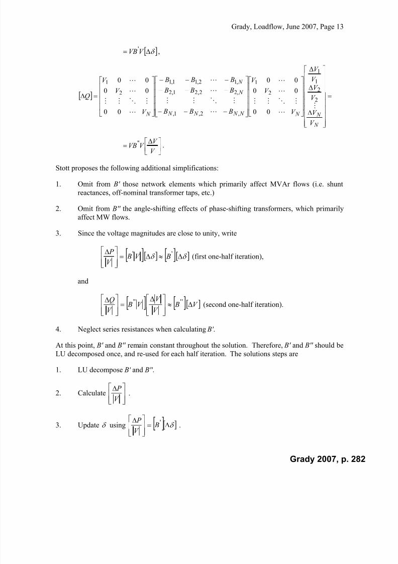
7/22/2019 Fundamentals Grady Notes June 2007 Print
http://slidepdf.com/reader/full/fundamentals-grady-notes-june-2007-print 282/388
Grady, Loadflow, June 2007, Page 13
V VB ' ,
N
N N N N N N
N
N
N
V
V
V
V
V
V
V
V
V
B B B
B B B
B B B
V
V
V
Q
2
2
1
1
2
1
,2,1,
,22,21,2
,12,11,1
2
1
00
00
00
00
00
00
V
V V VB '' .
Stott proposes the following additional simplifications:
1. Omit from B' those network elements which primarily affect MVAr flows (i.e. shunt
reactances, off-nominal transformer taps, etc.)
2. Omit from B'' the angle-shifting effects of phase-shifting transformers, which primarily
affect MW flows.
3. Since the voltage magnitudes are close to unity, write
'' BV BV
P (first one-half iteration),
and
V BV
V V B
V
Q
'''' (second one-half iteration).
4. Neglect series resistances when calculating B' .
At this point, B' and B'' remain constant throughout the solution. Therefore, B' and B'' should be
LU decomposed once, and re-used for each half iteration. The solutions steps are
1. LU decompose B' and B'' .
2. Calculate
V
P .
3. Update using
' BV
P .
Grady 2007, p. 282

7/22/2019 Fundamentals Grady Notes June 2007 Print
http://slidepdf.com/reader/full/fundamentals-grady-notes-june-2007-print 283/388
Grady, Loadflow, June 2007, Page 14
4. Check convergence, and continue if not converged.
5. Calculate
V
Q .
6. Update V using V BV
Q
''
7. Check convergence, and return to Step 2 if not converged.
5. Other Considerations
Current and Power Flow in Transmission Lines and Cables
Once the bus voltages throughout the system have been calculated, then the loadflow program
must calculate power flows through lines/transformers/cables. The standard pi-equivalentmodels are used for this purpose as follows:
R jX
Icapj Icapk
Ijk IkjVj/ j Vk/k
Q(pu)
2
Q(pu)
2 ,
so from side j, 0902
j jk k j j jk QV
jX R
V V I
,
and from side k, 0902
k k
j jk k kj
QV
jX R
V V I
.
Note that the current on the two opposite ends of the line are not exactly the same due to the fact
that the capacitor currents are not, in general, equal to each other.
The corresponding power flows for the two ends of the line are ** , kjkjkj jk jk jk I V S I V S .
Current and Power Flow in Transformers
The transformer equivalent circuit taken from Section 3 is
Grady 2007, p. 283

7/22/2019 Fundamentals Grady Notes June 2007 Print
http://slidepdf.com/reader/full/fundamentals-grady-notes-june-2007-print 284/388
Grady, Loadflow, June 2007, Page 15
y
Ijk IkjBus j
Bus k t / :1
Bus k'
Vj/ jVk/ k
,
so for side k, yt
V V I
j jk k kj
,
and for side j,
t
I I
kj jk .
The corresponding power flows for the two ends of the transformer are
** , kjkjkj jk jk jk I V S I V S .
Area Interchange
Large-scale power systems usually consist of several, or perhaps many, individual electric utility
companies. In these cases, each area may have a desired net input or output power to satisfy
sales and purchase agreements.
The area interchange feature in a loadflow program sums the tie-line flows into each area for a
net area power input. If these nets are not the desired values, to within a few megawatts, then an
area-control generator within the area is adjusted by the error amount. The sum of all input
powers for all areas must, of course, be zero.
Convergence Criteria
Most loadflow data cases are developed using a 100 MVA base, so that a 1% load corresponds to
1 MW. A typical convergence criteria is that the highest individual bus P and Q mismatches are
within 0.001 - 0.01%, or 0.00001 - 0.0001 pu.
Grady 2007, p. 284
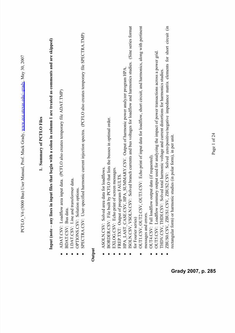
7/22/2019 Fundamentals Grady Notes June 2007 Print
http://slidepdf.com/reader/full/fundamentals-grady-notes-june-2007-print 285/388
P C F L O
_ V 6 ( 5 0 0 0 B u s ) U s e r M a n u a l ,
P r o f . M a c k G r a d y , w w w . e c e . u t e x a s . e d u / ~ g r a d y , M a y 3 0 , 2 0 0 7
P a g e 1 o f 2 4
1 . S u m m a r y o f P C F L O F i l e s
I n p u t ( n o t e – a n
y l i n e s i n i n p u t f i l e s t h a t b e g i n w i t h a c o l o n i n c o l u m n 1 a r e
t r e a t e d a s c o m m e n t s a n d a r e
s k i p p e d )
A D A T . C S V : L o a d f l o w a r e a i n p u t d a t a . ( P C F L
O a l s o c r e a t e s t e m p o r a r y f i l e A D A T . T M P )
B D A T . C S V : B u s d a t a .
L D A T . C S V : L i n e a n d t r a n s f o r m e r d a t a .
O P T I O N S . C S V
: S o l u t i o n o p t i o n s .
S P E C T R A . C S V
: U s e r - s p e c i f i e d h a r m o n i c c u r r e n t i n j e c t i o n s p e c t r a . ( P C F L O a
l s o c r e a t e s t e m p o r a r y f i l e S P E C
T R A . T M P )
O u t p u t
A S O L N . C S V : S o l v e d a r e a d a t a f o r l o a d f l o w s .
B O R D E R . C S V : F i l e b u i l t b y P C F L O t h a t l i s t s
t h e b u s s e s i n o p t i m a l o r d e r .
E X L O G . C S V : E c h o p r i n t o f s c r e e n m e s s a g e s .
F R E P . T X T : O u
t p u t o f p r o g r a m F A U L T S .
H P A_
L A S T_ C
A S E . C S V , H P A_ S
U M M A R Y . C
S V . O u t p u t o f h a r m o n i c p o w e r a n a l y z e r p r o g r a m H P A .
I S O L N . C S V , V S O L N . C S V : S o l v e d b r a n c h c u r r e n t s a n d b u s v o l t a g e s f o r l o a d f l o w a n d h a r m o n i c s s t u d i e s . ( S i n e s e r i e s f o r m a t
f o r F o u r i e r s e r i e
s )
O U T 1 . C S V , O U
T 2 . C S V , O U T 3 . C S V : E c h o p r
i n t o f i n p u t d a t a f o r l o a d f l o w , s h o r t c i r c u i t , a n d h a r m o n i c s , a l o n
g w i t h p e r t i n e n t
m e s s a g e s a n d e r r o r s .
O U T 4 . C S V : F u
l l l o a d f l o w o u t p u t d a t a ( i f r e q u e s t e d ) .
O U T 5 . C S V : L o a d f l o w s u m m a r y o u t p u t u s e d f o
r a n a l y z i n g t h e i m p a c t o f p o w e r t r a n s a c t i o n s a c r o s s a p o w e r g r i d .
T H D V . C S V , T H
D I . C S V : S o l v e d t o t a l h a r m o n i c v o l t a g e a n d c u r r e n t d i s t o r t i o n s f o r h a r m o n i c s s t u d i e s .
Z B U S 0 . C S V , Z
B U S 1 . C S V , Z B U S 2 . C S V : S o l v e d z e r o / p o s i t i v e / n e g a t i v e i m
p e d a n c e m a t r i x e l e m e n t s f o r s h o r t c i r c u i t ( i n
r e c t a n g u l a r f o r m
) o r h a r m o n i c s t u d i e s ( i n p o l a r f o r m ) , i n p e r u n i t .
Grady 2007, p. 285
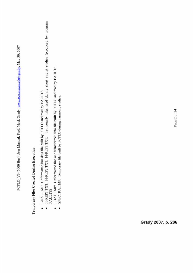
7/22/2019 Fundamentals Grady Notes June 2007 Print
http://slidepdf.com/reader/full/fundamentals-grady-notes-june-2007-print 286/388
P C F L O
_ V 6 ( 5 0 0 0 B u s ) U s e r M a n u a l ,
P r o f . M a c k G r a d y , w w w . e c e . u t e x a s . e d u / ~ g r a d y , M a y 3 0 , 2 0 0 7
P a g e 2 o f 2 4
T e m p o r a r y F i l e s C r e a
t e d D u r i n g E x e c u t i o n
B D A T . T M P : U
n f o r m a t t e d b u s d a t a f i l e b u i l t b y P C F L O a n d r e a d b y F A U L T S .
F F R E P 1 . T X T ,
F F R E P 2 . T X T , F F R E P 3 . T X T .
T e m p o r a r l y f i l e s u s e d d u r i n g s h o r t c i r c u i t s t u d i e s ( p r o d u c
e d b y p r o g r a m
F A U L T S )
L D A T . T M P : U
n f o r m a t t e d l i n e a n d t r a n s f o r m e r d a t a f i l e b u i l t b y P C F L O a n d r e a d b y F A U L T S .
S P E C T R A . T M P : T e m p o r a r y f i l e b u i l t b y P C F L
O d u r i n g h a r m o n i c s t u d i e s .
Grady 2007, p. 286

7/22/2019 Fundamentals Grady Notes June 2007 Print
http://slidepdf.com/reader/full/fundamentals-grady-notes-june-2007-print 287/388
P C F L O
_ V 6 ( 5 0 0 0 B u s ) U s e r M a n u a l ,
P r o f . M a c k G r a d y , w w w . e c e . u t e x a s . e d u / ~ g r a d y , M a y 3 0 , 2 0 0 7
P a g e 3 o f 2 4
2 . P r
e p a r e d C a s e s , R e a d y t o R u n
L o a d f l o w
5 B u s S t e v e n s o n * L o a d f l o w E x a m p l e , p p . 2 0 0 - 2 0 5 . F i l e E x t e n s i o n_ S
5 .
4 8 6 0 B u s L o a d f
l o w C a s e . F i l e E x t e n s i o n_
S C R
E W B E A N . U s e d f o r p o w e r g r i d s t u d i e s .
S h o r t C i r c u i t
6 B u s G r a i n g e r - S t e v e n s o n * * S h o r t C i r c u i t E x a m p l e ( P r o b . 3 . 1 2 , p . 1 3 9 , a n
d c o n t i n u e d w i t h P r o b . 1 1 . 1 7 , p . 4 6 9 ) . F i l e
E x t e n s i o n_ S
6
9 B u s G r a i n g e r - S t e v e n s o n * * S h o r t C i r c u i t E x a
m p l e ( P r o b . 3 . 1 3 , p p . 1 3 9 - 1 4 0 ,
a n d c o n t i n u e d w i t h P r o b . 1 1 . 1 8 , p . 4 6 9 ) . F i l e
E x t e n s i o n_ S
9 .
H a r m o n i c s
5 B u s T u t o r i a l .
F i l e E x t e n s i o n s_
F I V E a n d_ F I
V E_ F
I L T E R .
3 3 B u s A S D E x
a m p l e . F i l e E x t e n s i o n_ D
F W .
1 8 B u s O i l P i p e l i n e A S D E x a m p l e . F i l e E x t e n s
i o n_ P
I P E L I N E .
1 1 1 B u s 3 r d H a r m o n i c R e s o n a n c e E x a m p l e . F i l e E x t e n s i o n_ T
V .
1 7 B u s S m a l l S k i A r e a E x a m p l e . F i l e E x t e n s i o n s_ S
K I A ,_ S
K I B ,_ S
K I C .
4 5 4 B u s L a r g e S k i A r e a E x a m p l e . F i l e E x t e n s i o n s_ O
L Y M P I C S_ A
( u n f i l t e r e d
) ,_ O
L Y M P I C S_
D ( f i l t e r e d ) .
8 7 B u s D i s t r i b u t i o n E x a m p l e w i t h 3 r d H a r m o n i c
P r o b l e m D u e t o S i n g l e - P h a s e L
o a d s . F i l e E x t e n s i o n_ P
C .
*
W i l l i a m D . S t e v e n s o n , J r . ,
E l e m e n t s o f P o w e r S y s
t e m A n a l y s i s , F o u r t h E d i t i o n , M
c G r a w - H i l l , N e w Y o r k , 1 9 8 2 .
* *
J o h n J . G r a i n g e r , W i l l i a m D . S t e v e n s o n , J r . ,
P o w e
r S y s t e m A n a l y s i s , M c G r a w - H i l l , N e w Y o r k , 1 9 9 4 .
Grady 2007, p. 287

7/22/2019 Fundamentals Grady Notes June 2007 Print
http://slidepdf.com/reader/full/fundamentals-grady-notes-june-2007-print 288/388
P C F L O
_ V 6 ( 5 0 0 0 B u s ) U s e r M a n u a l ,
P r o f . M a c k G r a d y , w w w . e c e . u t e x a s . e d u / ~ g r a d y , M a y 3 0 , 2 0 0 7
P a g e 4 o f 2 4
3 . C
o n t e n t o f I n p u t D a t a F i l e s
B U S D A T A
( F i l e = B D A T . C
S V , o n e r e c o r d p e r b u s . C S V
f o r m a t )
V a r i a b l e
C o m m
e n t s
N u m b e r
I n t e g e r
N a m e
U p t o 1 2 c h a r a c t e r s
T y p e
1 = S w
i n g B u s
2 = P V
B u s
3 = P Q
B u s
L i n e a r P G e n e r a t i o n
P e r c e n
t
L i n e a r Q G e n e r a t i o n
P e r c e n
t
L i n e a r P L o a d
P e r c e n
t
L i n e a r Q L o a d
P e r c e n
t
D e s i r e d V o l t a g e
P e r u n i t
S h u n t R e a c t i v e Q L o a d
P e r c e n
t @ v o l t a g e = 1 p e r u n i t
M a x i m u m Q G e n e r a t i o n
P e r c e n
t
M i n i m u m Q G e n e r a t i o n
P e r c e n
t
C o n t r o l A r e a
I n t e g e r
Grady 2007, p. 288

7/22/2019 Fundamentals Grady Notes June 2007 Print
http://slidepdf.com/reader/full/fundamentals-grady-notes-june-2007-print 289/388
P C F L O
_ V 6 ( 5 0 0 0 B u s ) U s e r M a n u a l ,
P r o f . M a c k G r a d y , w w w . e c e . u t e x a s . e d u / ~ g r a d y , M a y 3 0 , 2 0 0 7
P a g e 5 o f 2 4
R e m o t e - C o n t r o l l e d B u s N u m b e r
U s e d f
o r c o n t r o l l i n g v o l t a g e a t a r e m o t e b u s . F o r t h e s e
c a s e s , t h e d e s i r e d v o l t a g e s p e c i f i e d a b o v e a p p l i e s t o t h e
r e m o t e
b u s .
C o n n e c t i o n T y p e f o r S h u n t R e a c t i v e Q L o a d
0 o r 1 = G r o u n d e d W y e .
O t h e r w
i s e , u n g r o u n d e d w y e o r d e l t a ( i . e . n o z e r o
s e q u e n
c e p a t h )
S u b t r a n s i e n t R , X ( P o s . S e q u e n c e )
S e r i e s
i m p e d a n c e o f m o t o r o r g e n e r a t o
r , i n p e r u n i t
S u b t r a n s i e n t R , X ( N e g
. S e q u e n c e )
S e r i e s
i m p e d a n c e o f m o t o r o r g e n e r a t o
r , i n p e r u n i t
S u b t r a n s i e n t R , X ( Z e r o
S e q u e n c e )
S e r i e s
i m p e d a n c e o f m o t o r o r g e n e r a t o
r , i n p e r u n i t
( i g n o r
i n g c o n n e c t i o n t y p e a n d g r o u n d
i n g i m p e d a n c e s )
( d o n o
t m u l t i p l y b y 3 )
C o n n e c t i o n T y p e f o r S u b t r a n s i e n t I m p e d a n c e s
0 o r 1 = G r o u n d e d W y e .
O t h e r w
i s e , u n g r o u n d e d w y e o r d e l t a ( i . e . n o z e r o
s e q u e n
c e p a t h )
G r o u n d i n g I m p e d a n c e R , X f o r S u b -
S e r i e s
i m p e d a n c e f r o m w y e p o i n t t o g r o u n d , i n p e r u n i t .
T r a n s i e n t I m p e d a n c e s
( d o n o t m u l t i p l y b y 3 ) .
N o n l i n e a r D e v i c e P G e n e r a t i o n
P G e n e r a t i o n t h a t c o m e s f r o m t h e n o n l i n e a r d e v i c e ,
i n p e r c
e n t .
N o n l i n e a r D e v i c e P L o a d
P L o a d
o f t h e n o n l i n e a r d e v i c e ,
i n p e r c
e n t .
N o n l i n e a r D e v i c e D i s p l a c e m e n t P o w e r F a c t o r
P e r U n
i t ( p o s i t i v e f o r l a g g i n g i s p o s i t i v e , n e g a t i v e f o r
l e a d i n g ) .
Grady 2007, p. 289

7/22/2019 Fundamentals Grady Notes June 2007 Print
http://slidepdf.com/reader/full/fundamentals-grady-notes-june-2007-print 290/388
P C F L O
_ V 6 ( 5 0 0 0 B u s ) U s e r M a n u a l ,
P r o f . M a c k G r a d y , w w w . e c e . u t e x a s . e d u / ~ g r a d y , M a y 3 0 , 2 0 0 7
P a g e 6 o f 2 4
N o n l i n e a r D e v i c e T y p e
1
=
2 - p u l s e c u r r e n t s o u r c e
2
=
2 - p u l s e v o l t a g e s o u r c e
3
=
6 - p u l s e c u r r e n t s o u r c e
4
=
6 - p u l s e v o l t a g e s o u r c e
5
=
1 2 - p u l s e c u r r e n t s o u r c e
6
=
1 2 - p u l s e v o l t a g e s o u r c e
7
=
1 8 - p u l s e c u r r e n t s o u r c e
8
=
1 8 - p u l s e v o l t a g e s o u r c e
9
=
D i v e r s i f i e d 6 - p u l s e c u r r e n t s o u
r c e ( l i k e
t y p e 3 , b u t w i t h t h e 1 1 & 1 3 t h h a r m o n i c s
m u l t i p l i e d b y 0 . 7 5 , t h e 1 7 & 1 9 t h h a r m o n i c s
b y 0 . 5 0 , a n d a l l h i g h e r h a r m o n i c s b y 0 . 2 5 )
1 0 =
S i n g l e - p h a s e e l e c t r o n i c G Y - G Y
1 1 =
S i n g l e - p h a s e e l e c t r o n i c D e l t a - G Y
1 2 =
M a g n e t i c f l u o r e s c e n t G Y - G Y
1 3 =
M a g n e t i c f l u o r e s c e n t D e l t a - G Y
1 4 =
U s e r - s p e c i f i e d t y p e 1 4
. . .
. . .
. . .
3 3 =
U s e r - s p e c i f i e d t y p e 3 3
N o n l i n e a r D e v i c e P h a s e S h i f t
D e g r e e s f o r p o s i t i v e s e q u e n c e , o n s y s t e m s i d e w i t h
r e s p e c t t o d e v i c e s i d e . T h i s i s t h e a d d i t i o n a l p h a s e s h i f t
b y w h i c h t h e c u r r e n t i n j e c t i o n p h a s e a n g l e s w i l l b e
a d v a n c e d f o r p o s i t i v e s e q u e n c e , a n d d e l a y e d f o r
n e g a t i v e s e q u e n c e .
C o n n e c t i o n T y p e f o r H a r m o n i c s M o d e l
0 o r 1 = G r o u n d e d W y e . O t h e r w i s e , u
n g r o u n d e d w y e
o f L i n e a r L o a d
o r d e l t a ( i . e . n o z e r o s e q u e n c e p a t h )
Grady 2007, p. 290
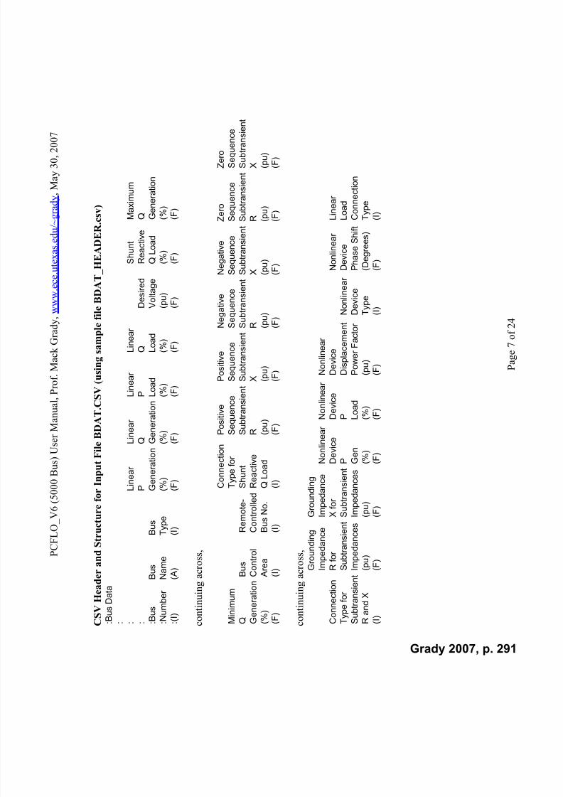
7/22/2019 Fundamentals Grady Notes June 2007 Print
http://slidepdf.com/reader/full/fundamentals-grady-notes-june-2007-print 291/388
P C F L O
_ V 6 ( 5 0 0 0 B u s ) U s e r M a n u a l ,
P r o f . M a c k G r a d y , w w w . e c e . u t e x a s . e d u / ~ g r a d y , M a y 3 0 , 2 0 0 7
P a g e 7 o f 2 4
C S V H e a d e r a n d S t r u
c t u r e f o r I n p u t F i l e B D A T . C S
V ( u s i n g s a m p l e f i l e B D A T_ H
E A D E R . c s v )
: B u s
D a
t a
: :
L i n e a r
L i n e a r
L i n e a r
L i n e a r
S h u n
t
M a x
i m u m
:
P
Q
P
Q
D e s
i r e d
R e a c
t i v e
Q
: B u s
B u s
B u s
G e n e r a
t i o n
G e n e r a
t i o n
L o a
d
L o a
d
V o
l t a g e
Q L o a
d
G e n e r a
t i o n
: N u m
b e r
N a m e
T y p e
( % )
( % )
( % )
( % )
( p u
)
( % )
( % )
: ( I )
( A )
( I )
( F )
( F )
( F )
( F )
( F )
( F )
( F )
c o n t i n u i n g a c r o s s ,
C o n n e c
t i o n
P o s
i t i v e
P o s
i t i v e
N e g a
t i v e
N e g a
t i v e
Z e r o
Z e r o
M i n i m u m
T y p e
f o r
S e q u e n c e
S e q u e n c e
S e q u e n c e
S e q u e n c e
S e q u e n c e
S e q u e n c e
Q
B u s
R
e m o
t e -
S h u n
t
S u
b t r a n s i e n
t S u
b t r a n s
i e n
t S u
b t r a n s
i e n
t S u b t r a n s
i e n
t S u
b t r a n s
i e n
t S u
b t r a n s i e n
t
G e n e r a
t i o n
C o n
t r o l
C
o n
t r o l l e d R e a c
t i v e
R
X
R
X
R
X
( % )
A r e a
B
u s
N o .
Q L o a
d
( p u
)
( p u
)
( p u
)
( p u
)
( p u
)
( p u
)
( F )
( I )
( I )
( I )
( F )
( F )
( F )
( F )
( F )
( F )
c o n t i n u i n g a c r o s s ,
G r o u n
d i n g
G r o u n
d i n g
I m p e
d a n c e
I m p e
d a n c e
N o n
l i n e a r
N o n l i n
e a r
N o n
l i n e a r
C o n n e c
t i o n
R f o r
X f o r
D e v
i c e
D e v i c e
D e v
i c e
N o n
l i n e a r
L i n e a r
T y p e
f o r
S u
b t r a n s i e
n t S u
b t r a n s
i e n
t P
P
D i s p
l a c e m e n
t
N o n
l i n e a r
D e v
i c e
L o a
d
S u
b t r a n s
i e n
t I m p e
d a n c e
s
I m p e
d a n c e s
G e n
L o a
d
P o w e r
F a c
t o r
D e v
i c e
P h a s e
S h i f t C o n n e c
t i o n
R a n
d X
( p u
)
( p u
)
( % )
( % )
( p u
)
T y p e
( D
e g r e e s
)
T y p e
( I )
( F )
( F )
( F )
( F )
( F )
( I )
( F
)
( I )
Grady 2007, p. 291
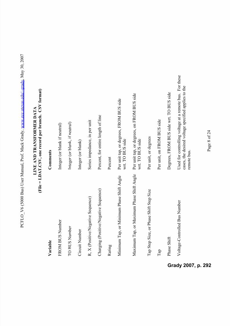
7/22/2019 Fundamentals Grady Notes June 2007 Print
http://slidepdf.com/reader/full/fundamentals-grady-notes-june-2007-print 292/388
P C F L O
_ V 6 ( 5 0 0 0 B u s ) U s e r M a n u a l ,
P r o f . M a c k G r a d y , w w w . e c e . u t e x a s . e d u / ~ g r a d y , M a y 3 0 , 2 0 0 7
P a g e 8 o f 2 4
L I N E A
N D T R A N S F O R M E R D A T A
( F i l e = L D A T . C S
V , o n e r e c o r d p e r b r a n c h . C S
V f o r m a t )
V a r i a b l e
C o m
m e n t s
F R O M B U S N u m b e r
I n t e g
e r ( o r b l a n k i f n e u t r a l )
T O B U S N u m b e r
I n t e g
e r ( o r b l a n k , i f n e u t r a l )
C i r c u i t N u m b e r
I n t e g
e r ( o r b l a n k )
R , X ( P o s i t i v e / N e g a t i v e S e q u e n c e )
S e r i e
s i m p e d a n c e , i n p e r u n i t
C h a r g i n g ( P o s i t i v e / N e g
a t i v e S e q u e n c e )
P e r c e n t , f o r e n t i r e l e n g t h o f l i n e
R a t i n g
P e r c e n t
M i n i m u m T a p , o r M i n i m u m P h a s e S h i f t A n g l e
P e r u
n i t t a p , o r d e g r e e s , F R O M B U S
s i d e
w r t . T O B U S s i d e
M a x i m u m T a p , o r M a x i m u m P h a s e S h i f t A n g l e
P e r u
n i t t a p , o r d e g r e e s , o n F R O M B
U S s i d e
w r t . T O B U S s i d e
T a p S t e p S i z e , o r P h a s e
S h i f t S t e p S i z e
P e r u
n i t , o r d e g r e e s
T a p
P e r u
n i t , o n F R O M B U S s i d e
P h a s e S h i f t
D e g r e e s , F R O M B U S s i d e w r t . T O B
U S s i d e
V o l t a g e - C o n t r o l l e d B u s N u m b e r
U s e d
f o r c o n t r o l l i n g v o l t a g e a t a r e m
o t e b u s . F o r t h e s e
c a s e s , t h e d e s i r e d v o l t a g e s p e c i f i e d a
p p l i e s t o t h e
r e m o
t e b u s .
Grady 2007, p. 292

7/22/2019 Fundamentals Grady Notes June 2007 Print
http://slidepdf.com/reader/full/fundamentals-grady-notes-june-2007-print 293/388
P C F L O
_ V 6 ( 5 0 0 0 B u s ) U s e r M a n u a l ,
P r o f . M a c k G r a d y , w w w . e c e . u t e x a s . e d u / ~ g r a d y , M a y 3 0 , 2 0 0 7
P a g e 9 o f 2 4
V o l t a g e - C o n t r o l l e d B u s S i d e
W h e
n c o n t r o l l i n g t h e v o l t a g e a t a r e m o t e b u s , e n t e r 1
w h e n t h e r e m o t e b u s i s o n t h e F R O M
B U S s i d e o f t h e
t r a n s
f o r m e r . E n t e r 2 w h e n t h e r e m o t e b u s i s o n t h e
T O B
U S s i d e o f t h e t r a n s f o r m e r .
D e s i r e d V o l t a g e f o r V o
l t a g e - C o n t r o l l e d B u s ,
P e r u
n i t V o l t a g e , o r P e r c e n t A c t i v e P
o w e r ( F R O M B U S
o r D e s i r e d A c t i v e P o w e r F l o w f o r P h a s e
t o w a
r d T O B U S )
S h i f t i n g T r a n s f o r m e r
R , X ( Z e r o S e q u e n c e )
S e r i e
s i m p e d a n c e , i n p e r u n i t ( i g n o r i
n g c o n n e c t i o n t y p e
a n d g r o u n d i n g i m p e d a n c e s ) , ( d o n o t
m u l t i p l y b y 3 )
C h a r g i n g ( Z e r o S e q u e n
c e )
P e r c e n t , f o r e n t i r e l e n g t h o f l i n e
C o n n e c t i o n T y p e f o r T r a n s f o r m e r s a n d
F o r t r a n s f o r m e r s :
S h u n t E l e m e n t s
T y p e
F R O M B U S
T O B U S
0 o r 1
G Y
G Y
2
G Y
Y
3
Y
G Y
4
Y
Y
5
6
G Y
7
Y
8
G Y
9
Y
F o r s h u n t e l e m e n t s :
0 o r 1 = G r o u n d e d W y e .
O t h e
r w i s e , u n g r o u n d e d w y e o r d e l t a
( i . e . n o z e r o
s e q u e n c e p a t h )
G r o u n d i n g I m p e d a n c e R , X
S e r i e s i m p e d a n c e f r o m w y e p o i n t t o
g r o u n d , i n p e r u n i t
A p p l i e s t o w y e - c o n n e c t e d t r a n s f o r m e r s a n d s h u n t
Grady 2007, p. 293

7/22/2019 Fundamentals Grady Notes June 2007 Print
http://slidepdf.com/reader/full/fundamentals-grady-notes-june-2007-print 294/388
P C F L O
_ V 6 ( 5 0 0 0 B u s ) U s e r M a n u a l ,
P r o f . M a c k G r a d y , w w w . e c e . u t e x a s . e d u / ~ g r a d y , M a y 3 0 , 2 0 0 7
P a g e 1 0 o f 2 4
e l e m
e n t s . ( d o n o t m u l t i p l y b y 3 )
R e s i s t i v e S k i n E f f e c t F a c t o r f o r
H a r m
o n i c h ( h > 2 , f r a c t i o n a l v a l u e s
O K ) a t w h i c h
P o s i t i v e / N e g a t i v e S e q u e n c e
t h e c
o n d u c t o r r e s i s t a n c e i s d o u b l e t h
e f u n d a m e n t a l
f r e q u
e n c y r e s i s t a n c e .
R e s i s t i v e S k i n E f f e c t F a c t o r f o r
H a r m
o n i c h ( h > 2 , f r a c t i o n a l v a l u e s
O K ) a t w h i c h
Z e r o S e q u e n c e
t h e c
o n d u c t o r r e s i s t a n c e i s d o u b l e t h e f u n d a m e n t a l
f r e q u
e n c y r e s i s t a n c e . T h i s v a l u e a p p
l i e s t o t h e
c o m b i n e d c o n d u c t o r a n d g r o u n d i n g r e s i s t a n c e .
Grady 2007, p. 294

7/22/2019 Fundamentals Grady Notes June 2007 Print
http://slidepdf.com/reader/full/fundamentals-grady-notes-june-2007-print 295/388
P C F L O
_ V 6 ( 5 0 0 0 B u s ) U s e r M a n u a l ,
P r o f . M a c k G r a d y , w w w . e c e . u t e x a s . e d u / ~ g r a d y , M a y 3 0 , 2 0 0 7
P a g e 1 1 o f 2 4
H e a d e r a n d S t r u c t u r e
f o r I n p u t F i l e L D A T . C S V ( u s i n g s a m p l e f i l e L D A T_ H
E A D
E R . c s v )
: L i n e a n
d T r a n s
f o r m e r D a
t a
: : : :
P o s
i t i v e
P o s
i t i v e
P o s
/ N e g
:
S e q u e n c e
S e q u e n c e
S e q u e n c e
M i n i m u m
M
a x
i m u m
T a p
F i x e
d
: F r o m
T o
C
i r c u
i t
R
X
C
h a r g
i n g
R a
t i n g
T a p
T a p
S t e p
S i z e
T a p
: B u s
B u s
N
u m
b e r
( p u
)
( p u
)
( %
)
( % )
( p u
)
( p
u )
( p u
)
( p u
)
: ( I )
( I )
( I )
( F )
( F )
( F
)
( F )
( F )
( F
)
( F )
( F )
c o n t i n u i n g a c r o s s ,
D e s
i r e d V o
l t a g e
a t V o
l t a g e
C o n
t . B u s
( p u
)
C o n n e c
t .
V o
l t a g e -
V o
l t a g e -
o r
D e s
i r e d P
Z e r o
Z e r o
Z e r o
T y p e
S e r i e s
S e r i e s
P h a s e
C o n
t .
C o n
t .
f o r
S e q u e n c e
S e q u e n c e
S e q u e n c e
f o r
T r a n s .
G r o u n
d i n g
G r o u n
d i n g
S h i f t
B u s
B u s
P h a s e
S h i f t e r
R
X
C h a r g
i n g
a n
d S h
u n
t R
X
( D e g r e e s
) N u m
b e r
S i d e
( % )
( p u
)
( p u
)
( % )
E l e m e n
t s
( p u
)
( p u
)
( F )
( I )
( I )
( F )
( F )
( F )
( F )
( I )
( F )
( F )
Grady 2007, p. 295

7/22/2019 Fundamentals Grady Notes June 2007 Print
http://slidepdf.com/reader/full/fundamentals-grady-notes-june-2007-print 296/388
P C F L O
_ V 6 ( 5 0 0 0 B u s ) U s e r M a n u a l ,
P r o f . M a c k G r a d y , w w w . e c e . u t e x a s . e d u / ~ g r a d y , M a y 3 0 , 2 0 0 7
P a g e 1 2 o f 2 4
A R E
A I N T E R C H A N G E D A T A
( F i l e = A D A T . C S V , o n e r e c o r d p e r l o a d f l o w a r e a .
C S V f o r m a t )
V a r i a b l e
C o m m
e n t s
N u m b e r
I n t e g e r
T i e - L i n e L o s s A s s i g n m
e n t
I f n o n - z e r o , t h e n p o w e r l o s s e s o n t i e l i n e s a r e a s s i g n e d
e q u a l l y b e t w e e n t h e t w o a r e a s . I f z e r o
, t h e T O B U S
a r e a f o
r e a c h t i e l i n e i s a s s i g n e d t h e l o s s ( i . e . , m e t e r a t
t h e F R
O M B U S ) .
C o n t r o l B u s N u m b e r
I n t e g e r
D e s i r e d E x p o r t P o w e r
P e r c e n
t
S o l u t i o n T o l e r a n c e f o r E x p o r t
P e r c e n
t
N a m e
U p t o 2 0 c h a r a c t e r s
Grady 2007, p. 296

7/22/2019 Fundamentals Grady Notes June 2007 Print
http://slidepdf.com/reader/full/fundamentals-grady-notes-june-2007-print 297/388
P C F L O
_ V 6 ( 5 0 0 0 B u s ) U s e r M a n u a l ,
P r o f . M a c k G r a d y , w w w . e c e . u t e x a s . e d u / ~ g r a d y , M a y 3 0 , 2 0 0 7
P a g e 1 3 o f 2 4
H e a d e r a n d S t r u c t u r e
f o r I n p u t F i l e A D A T . C S V ( u s i n g s a m p l e f i l e A D A T_ H
E A D
E R . c s v )
: A r e a
I n t e r c
h a n g e
D a
t a
:
T i e L i n e
:
L o s s
:
A s s
i g n m .
:
( 1 f o r
:
S p
l i t t i n g ,
D e s
i r e d
S o
l u t i o n
:
0 f o r
T o
C
o n
t r o l
E x p o r t
T o
l e r a n c e
: A r e a
B u s
B u s
P o w e r
f o r
E x p o r t
A r e a
: N u m
b e r
O w n e r s
h i p N
u m
b e r
( % )
( % )
N
a m e
: ( I )
( I )
( I )
( F )
( F )
( A
)
Grady 2007, p. 297
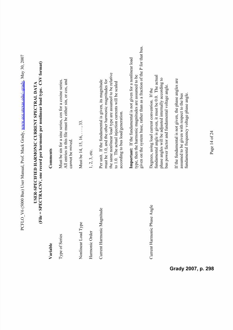
7/22/2019 Fundamentals Grady Notes June 2007 Print
http://slidepdf.com/reader/full/fundamentals-grady-notes-june-2007-print 298/388
P C F L O
_ V 6 ( 5 0 0 0 B u s ) U s e r M a n u a l ,
P r o f . M a c k G r a d y , w w w . e c e . u t e x a s . e d u / ~ g r a d y , M a y 3 0 , 2 0 0 7
P a g e 1 4 o f 2 4
U S E R - S P E C I F I E D H
A R M O N I C C U R R E N T S P E C
T R A L D A T A
( F i l e = S P E C T R A . C S V , o n e r e c o
r d p e r h a r m o n i c p e r n o n l i n e a
r l o a d t y p e . C S V f o r m a t )
V a r i a b l e
C o
m m e n t s
T y p e o f S e r i e s
M u s t b e s i n f o r a s i n e s e r i e s , c o s f o r a c o s i n e s e r i e s .
A l l e n t r i e s i n t h i s f i l e m u s t b e e i t h e r s i n , o r c o s , a n d
c a n n o t b e m i x e d .
N o n l i n e a r L o a d T y p e
M u s t b e 1 4 , 1 5 , 1 6 , . . . , 3 3 .
H a r m o n i c O r d e r
1 , 2 , 3 , e t c .
C u r r e n t H a r m o n i c M a g n i t u d e
P e r u n i t . I f t h e f u n d a m e n t a l i s g i v e n , i t s m a g n i t u d e
m u
s t b e 1 . 0 , a n d t h e o t h e r h a r m o n i c m a g n i t u d e s f o r
t h e
s a m e n o n l i n e a r l o a d t y p e a r e a s s u m e d t o b e r e l a t i v e
t o 1 . 0 . T h e a c t u a l i n j e c t i o n c u r r e n t s w i l l b e s c a l e d
a c c o r d i n g t o b u s l o a d / g e n e r a t i o n .
I m
p o r t a n t : I f t h e f u n d a m e n t a l i s n o t g i v e n f o r a n o n l i n e a r l o a d
t y p
e , t h e n t h e h a r m o n i c m a g n i t u d e
s a r e a s s u m e d t o b e
g i v
e n o n t h e s y s t e m b a s e , r a t h e r t h
a n a s a f r a c t i o n o f t h e P f o r t h a t
b u s .
C u r r e n t H a r m o n i c P h a s
e A n g l e
D e
g r e e s , u s i n g l o a d c u r r e n t c o n v e n t i o n . I f t h e
f u n
d a m e n t a l a n g l e i s g i v e n , i t m u s t b e 0 . 0 . T h e a c t u a l
p h a s e a n g l e s w i l l b e a d j u s t e d i n t e r n a l l y a c c o r d i n g t o
b u s p o w e r f a c t o r a n d f u n d a m e n t a l
v o l t a g e a n g l e .
I f t h e f u n d a m e n t a l i s n o t g i v e n , t h e
p h a s e a n g l e s a r e
a s s
u m e d t o b e g i v e n w i t h r e s p e c t t o t h e b u s
f u n
d a m e n t a l f r e q u e n c y v o l t a g e p h a s e a n g l e .
Grady 2007, p. 298

7/22/2019 Fundamentals Grady Notes June 2007 Print
http://slidepdf.com/reader/full/fundamentals-grady-notes-june-2007-print 299/388
P C F L O
_ V 6 ( 5 0 0 0 B u s ) U s e r M a n u a l ,
P r o f . M a c k G r a d y , w w w . e c e . u t e x a s . e d u / ~ g r a d y , M a y 3 0 , 2 0 0 7
P a g e 1 5 o f 2 4
H e a d e r a n d S t r u c t u r e
f o r I n p u t F i l e S P E C T R A . C S V ( u s i n g s a m p l e f i l e S P E C T R A
_ H E A D E R . c s v )
: H a r m o n
i c C u r r e n
t S p e c
t r a l D a
t a
:
C u r r e n
t
: T y p e o
f
C u r r e n
t
H a r m o n
i c
: S e r i e s
N o n
l i n e a r
H
a r m o n
i c
H a r m o n
i c
P h a s e
: ( S I N o r
L o a
d
O
r d e r
M a g .
A n g
l e
: C O S )
T y p e
( I n
t e g e r )
( p u
)
( D e g r e e s
)
: ( A )
( I )
( I )
( F )
( F )
Grady 2007, p. 299

7/22/2019 Fundamentals Grady Notes June 2007 Print
http://slidepdf.com/reader/full/fundamentals-grady-notes-june-2007-print 300/388
P C F L O
_ V 6 ( 5 0 0 0 B u s ) U s e r M a n u a l ,
P r o f . M a c k G r a d y , w w w . e c e . u t e x a s . e d u / ~ g r a d y , M a y 3 0 , 2 0 0 7
P a g e 1 6 o f 2 4
S O L U T I O N O P T I O N S
( F i l e = O P T I O N S . C S V . C S V f o r m a t . )
F o r L o a d f l o w ( u s i n g s
a m p l e f i l e O P T I O N S_ H
E A D E
R_ L
O A D F L O W . c s v )
L o a
d f l o w
S t u d y
C a s e - U
s e r
T i t l e G o e s o n
T h i s L i n e
: L o a
d f l o w
S o
l u t i o n
O p
t i o n s
:
V o
l t a g e
D i s a
b l e
: O p
t i m a
l
P
& Q
A c c e
l .
U p
d a
t e
D i s a
b l e
T r a n s
f .
: B u s
M
i s m a
t c h
F a c
t o r
C a p
P & Q
R e m o
t e
D i s a
b l e
I g n
o r e
T a p
: O r d e r i n g
G a u s s -
f o
r G a u s s -
f o r
G a u s s -
f o r
G a u s s -
M i s m a
t c h
V o
l t . R e g .
A r e a
Q L i m i t s
A d j u s
t . f o r
: M e
t h o
d
S e
i d e
l
S e
i d e
l
S e
i d e
l
S e
i d e
l
S o
l u t i o n
b y
P V
I n t r c h n g e
o n
P V
V o
l t a g e
: ( I n t e g e r )
S t a r t ?
S t a r t
S t a r t
S t a r t
T o
l e r a n c e
B u s s e s
?
P A d j u s
t ?
B u
s s e s
?
C o n
t r o l ?
: ( 1 - 2 - 3
)
( T o r
F )
( 0
. 5 p u
)
( 1 . 2
p u
)
( 0 . 0
0 5 p u
) ( 5 E - 0
6 p u
) ( T o r
F )
( T o r
F )
( T
o r
F )
( T o r
F )
: ( I )
( L )
( F
)
( F )
( F )
( F )
( L )
( L )
( L )
( L )
2 T
0 . 5
1 . 2
0 . 0
0 5 5
. 0 0 E - 0
6 F
F
F
F
c o n t i n u i n g a c r o s s ,
L i m i t
O u
t p u
t
a n
d
a n
d
a n
d
a n
d
t o T h i s
T h i s
T h i s
T h i s
T h i s
C o n
t r o l
C o n
t r o l
C
o n
t r o l
C o n
t r o l
C o n
t r o l
A r e a
?
A r e a
?
A r e a
?
A r e a
?
A r e a
?
( I n t e g e r )
( I n t e g e r )
( I n
t e g e r )
( I n t e g e r )
( I n t e g e r )
( I )
( I )
( I )
( I )
( I )
0
0
0
0
0
Grady 2007, p. 300
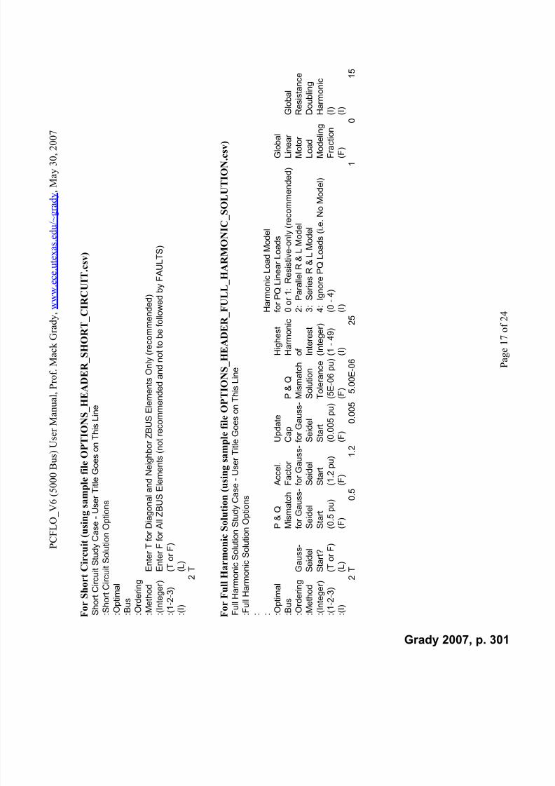
7/22/2019 Fundamentals Grady Notes June 2007 Print
http://slidepdf.com/reader/full/fundamentals-grady-notes-june-2007-print 301/388
P C F L O
_ V 6 ( 5 0 0 0 B u s ) U s e r M a n u a l ,
P r o f . M a c k G r a d y , w w w . e c e . u t e x a s . e d u / ~ g r a d y , M a y 3 0 , 2 0 0 7
P a g e 1 7 o f 2 4
F o r S h o r t C i r c u i t ( u s i n g s a m p l e f i l e O P T I O N S_
H E A D E R_ S
H O R T_ C
I R C U I T . c s v )
S h o r t C i r c u i t S t u d y C a s e
- U s e r T i t l e G o e s o n T h i s L i n e
: S h o r t C i r c u i t S o l u t i o n O p t i o n s
: O p t i m a l
: B u s
: O r d e r i n g
: M e t h o d
E n t e r T f o r D i a g o n a l a n d N e i g h b o r Z B U S E l e m e
n t s O n l y ( r e c o m m e n d e d )
: ( I n t e g e r )
E n t e r F f o r A l l Z B U S E l e m e n t s ( n o t r e c o m m e n d
e d a n d n o t t o b e f o l l o w e d b y F A U L
T S )
: ( 1 - 2 - 3 )
( T o r F )
: ( I )
( L )
2 T
F o r F u l l H a r m o n i c S o
l u t i o n ( u s i n g s a m p l e f i l e O P T I O N S_
H E A D E R_ F
U L L_ H
A R
M O N I C_ S
O L U T I O N . c s v )
F u
l l H a r m o n
i c S o
l u t i o n S
t u d y
C a s e -
U s e r
T i t l e G o e s o n
T h i s L i n e
: F u
l l H a r m o n
i c S o
l u t i o n O
p t i o n s
: :
H a r m o n
i c L o a
d M o
d e
l
: O p
t i m a
l
P
& Q
A c c e
l .
U p
d a
t e
H i g h e s
t
f o r
P Q L i n e a r
L o a
d s
G l o b a l
: B u s
M
i s m a
t c h
F a c
t o r
C a p
P & Q
H a r m o n
i c
0 o r
1 :
R e s i s t
i v e - o n
l y ( r e c o m m e n
d e
d )
L i n e a r
G l o b a
l
: O r d e r i n g
G a u s s -
f o
r G a u s s -
f o r
G a u s s -
f o r
G a u s s -
M i s m a
t c h
o f
2 :
P a r a
l l e l R & L M o
d e
l
M o
t o r
R e s
i s t a n c e
: M e
t h o
d
S e
i d e
l
S e
i d e
l
S e
i d e
l
S e
i d e
l
S o
l u t i o n
I n t e r e s
t
3 :
S e r i e s
R &
L M o
d e
l
L o a
d
D o u
b l i n g
: ( I n t e g e r )
S t a r t ?
S t a r t
S t a r t
S t a r t
T o
l e r a n c e
( I n t e g e r )
4 :
I g n o r e
P Q
L o a
d s
( i . e .
N o
M o
d e
l )
M o
d e l i n g
H a r m o n
i c
: ( 1 - 2 - 3
)
( T o r
F )
( 0
. 5 p u
)
( 1 . 2
p u
)
( 0 . 0
0 5 p u
) ( 5 E - 0
6 p u
) ( 1 -
4 9 )
( 0 -
4 )
F r a c
t i o n
( I )
: ( I )
( L )
( F
)
( F )
( F )
( F )
( I )
( I )
( F )
( I )
2 T
0 . 5
1 . 2
0 . 0
0 5 5
. 0 0 E - 0
6
2 5
1
0
1 5
Grady 2007, p. 301

7/22/2019 Fundamentals Grady Notes June 2007 Print
http://slidepdf.com/reader/full/fundamentals-grady-notes-june-2007-print 302/388
P C F L O
_ V 6 ( 5 0 0 0 B u s ) U s e r M a n u a l ,
P r o f . M a c k G r a d y , w w w . e c e . u t e x a s . e d u / ~ g r a d y , M a y 3 0 , 2 0 0 7
P a g e 1 8 o f 2 4
F o r H a r m o n i c I m p e d a n c e S c a n ( u s i n g s a m p l e f i l e O
P T I O N S_
H E A D E R_ H
A R M O
N I C_ I
M P E D A N C E_
S C A N . c s v )
H a r m o n
i c I m p e
d a n c e
S c
a n
S t u d y
C a s e -
U s e r
T i t l e G o e s o n
T h i s L i n e
: H a r m o n
i c I m p e
d a n c e
S c a n
: : O p
t i m a
l
P
& Q
A c c e
l .
U p
d a
t e
L o w e s
t
H i g h e s
t
N u
m b e r
L i m i t t h e
: B u s
M
i s m a
t c h
F a c
t o r
C a p
P & Q
H a r m o n
i c
H a r m o n
i c
o f
S t e p s
O u
t p u
t t o
: O r d e r i n g
G a u s s -
f o
r G a u s s -
f o r
G a u s s -
f o r
G a u s s -
M i s m a
t c h
o f
o f
p e r
D i a g o n a
l
: M e
t h o
d
S e
i d e
l
S e
i d e
l
S e
i d e
l
S e
i d e
l
S o
l u t i o n
I n t e r e s
t
I n t e r e s
t
H a
r m o n
i c
E l e m e n
t s
: ( I n t e g e r )
S t a r t ?
S t a r t
S t a r t
S t a r t
T o
l e r a n c e
( I n t e g e r )
( I n t e g e r )
( I n
t e g e r )
O n
l y ?
: ( 1 - 2 - 3
)
( T o r
F )
( 0
. 5 p u
)
( 1 . 2
p u
)
( 0 . 0
0 5 p u
) ( 5 E - 0
6 p u
) ( 1 -
4 9 )
( 1 -
4 9 )
( 1
- 1 0 0 )
( T o r
F )
: ( I )
( L )
( F
)
( F )
( F )
( F )
( I )
( I )
( I )
( L )
c o n t i n u i n g a c r o s s ,
H a r m o n i c L o a d M o d e l
f o r P Q L
i n e a r L o a d s
G l o b a l
0 o r 1 : R e s i s t i v e - o n l y ( r e c o m m e n d e d )
L i n e a r
G l o b a l
S c a n
a n d
a n d
a n d
a n d
2 :
P a r a l l e l R
& L M o d e l
M o t o r
R e s i s t a n c e
T h i s
T h i s
T h i s
T h i s
T h i s
3 :
S e r i e s R
& L M o d e l
L o a d
D o u b l i n g
B u s
B u s
B u s
B u s
B u s
4 :
I g n o r e P Q L o a d s ( i . e . N o M o d e l )
M o d e l i n g
H a r m o n i c
( I n t e g e r )
( I n t e g e r )
( I n t e g e r )
( I n t e g e r )
( I n t e g e r )
( 0
- 4 )
F r a c t i o n
( I )
( I )
( I )
( I )
( I )
( I )
( I )
( F )
( I )
Grady 2007, p. 302

7/22/2019 Fundamentals Grady Notes June 2007 Print
http://slidepdf.com/reader/full/fundamentals-grady-notes-june-2007-print 303/388
P C F L O
_ V 6 ( 5 0 0 0 B u s ) U s e r M a n u a l ,
P r o f . M a c k G r a d y , w w w . e c e . u t e x a s . e d u / ~ g r a d y , M a y 3 0 , 2 0 0 7
P a g e 1 9 o f 2 4
4 . H a r m o n i c - R e l a t
e d a n d S h o r t - C i r c u i t R e l a t e d O u t p u t F i l e s
( N o t e - f o r l o a d f l o w s t u d i e s , t h e f o r m a t s o f I S O L N a n
d V S O L N a r e d i f f e r e n t f r o m b e l o w b u t a r e s e l f - e x p l a n a t o r y w h e n v i e w i n g t h e
f i l e s . F o r s h o r t c i r c u i t s t u d i e s , t h e Z B U S f i l e s a r e s i m i l a r t o b e l o w , b u t w r i t t e n i n r e c t a n g u l a r f o r m )
C o m m a s s e p a r a t e t h e f i
e l d s s h o w n b e l o w t o f a c i l i t a t e t h e i r u s e w i t h M i c r o s o f t E x c e l .
I S O L N . C S V ( f o r h a r m
o n i c s )
D a t a F i e l d
( s t a r t i n g f r o m
t h e l e f t )
D e s c r i p t i o n
1
H a r m o n i c n u m b e r
2
F r o m b u s n u m b e r
3
T o b u s n u m b e r
4
C i r c u i t n u m b e r
5
C u r r e n t m a g n i t u d e - p
e r u n i t
6
C u r r e n t p h a s e a n g l e ( s i n e r e f e r e n c e ) - d e g r e e s
7
F r o m b u s n a m e ( a t t h e f i r s t o p p o r t u n i t y o n l y )
8
T o b u s n a m e ( a t t h e f i r s t o p p o r t u n i t y o n l y )
9
L o a d i n g l e v e l - p e r c e n t o f l i n e r a t i n g ( f o r
f u n d a m e n t a l f r e q u e n c
y o n l y )
V S O L N . C S V ( f o r h a r m o n i c s )
D a t a F i e l d
( s t a r t i n g f r o m
t h e l e f t )
D e s c r i p t i o n
1
H a r m o n i c n u m b e r
2
B u s n u m b e r
3
V o l t a g e m a g n i t u d e - p e r u n i t
Grady 2007, p. 303

7/22/2019 Fundamentals Grady Notes June 2007 Print
http://slidepdf.com/reader/full/fundamentals-grady-notes-june-2007-print 304/388
P C F L O
_ V 6 ( 5 0 0 0 B u s ) U s e r M a n u a l ,
P r o f . M a c k G r a d y , w w w . e c e . u t e x a s . e d u / ~ g r a d y , M a y 3 0 , 2 0 0 7
P a g e 2 0 o f 2 4
4
V o l t a g e p h a s e a n g l e ( s i n e r e f e r e n c e ) - d e g r e e s
5
N o n l i n e a r d e v i c e l o a d
c u r r e n t m a g n i t u d e -
p e r u n i t
6
N o n l i n e a r d e v i c e l o a d
c u r r e n t p h a s e a n g l e
( s i n e r e f e r e n c e ) - d e g r e e s
7
B u s n a m e ( a t t h e f i r s t
o p p o r t u n i t y o n l y )
Z B U S 0 . C S V , Z B U S 1 . C S V , Z B U S 2 . C S V ( f o r h a r m o n i c s a n d s h o r t c i r c u i t )
D a t a F i e l d
( s t a r t i n g f r o m
t h e l e f t )
D e s c r i p t i o n
1
H a r m o n i c n u m b e r
2
F r o m b u s n u m b e r
3
T o b u s n u m b e r
4
I m p e d a n c e m a g n i t u d e - p e r u n i t
5
I m p e d a n c e p h a s e a n g l e - d e g r e e s
6
F r o m b u s n a m e ( a t t h e f i r s t o p p o r t u n i t y o n l y )
7
T o b u s n a m e ( a t t h e f i r s t o p p o r t u n i t y o n l y )
T H D V . C S V ( f o r h a r m
o n i c s )
C o n t a i n s a l i s t o
f b u s n u m b e r s w i t h t h e i r c o r r e s p o n d i n g n a m e s a n d v o l t a g e d i s t o r t i o n s .
Grady 2007, p. 304

7/22/2019 Fundamentals Grady Notes June 2007 Print
http://slidepdf.com/reader/full/fundamentals-grady-notes-june-2007-print 305/388
P C F L O
_ V 6 ( 5 0 0 0 B u s ) U s e r M a n u a l ,
P r o f . M a c k G r a d y , w w w . e c e . u t e x a s . e d u / ~ g r a d y , M a y 3 0 , 2 0 0 7
P a g e 2 1 o f 2 4
E x a m p
l e S c r e e n s f o r t h e_ D
F W C a s e
Grady 2007, p. 305

7/22/2019 Fundamentals Grady Notes June 2007 Print
http://slidepdf.com/reader/full/fundamentals-grady-notes-june-2007-print 306/388
P C F L O
_ V 6 ( 5 0 0 0 B u s ) U s e r M a n u a l ,
P r o f . M a c k G r a d y , w w w . e c e . u t e x a s . e d u / ~ g r a d y , M a y 3 0 , 2 0 0 7
P a g e 2 2 o f 2 4
Grady 2007, p. 306

7/22/2019 Fundamentals Grady Notes June 2007 Print
http://slidepdf.com/reader/full/fundamentals-grady-notes-june-2007-print 307/388
P C F L O
_ V 6 ( 5 0 0 0 B u s ) U s e r M a n u a l ,
P r o f . M a c k G r a d y , w w w . e c e . u t e x a s . e d u / ~ g r a d y , M a y 3 0 , 2 0 0 7
P a g e 2 3 o f 2 4
Grady 2007, p. 307
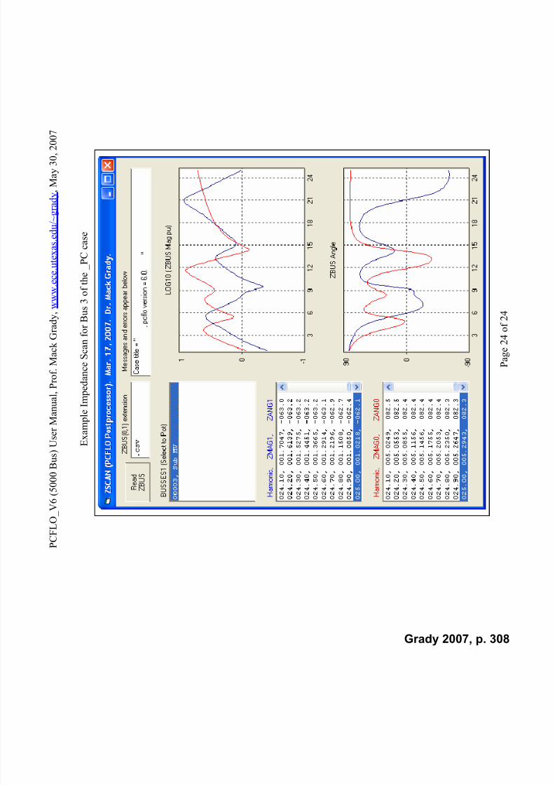
7/22/2019 Fundamentals Grady Notes June 2007 Print
http://slidepdf.com/reader/full/fundamentals-grady-notes-june-2007-print 308/388
P C F L O
_ V 6 ( 5 0 0 0 B u s ) U s e r M a n u a l ,
P r o f . M a c k G r a d y , w w w . e c e . u t e x a s . e d u / ~ g r a d y , M a y 3 0 , 2 0 0 7
P a g e 2 4 o f 2 4
E x a m p l e I m p e d a n c e S c a n f o r B u s 3 o f t h e_ P
C c a s e
Grady 2007, p. 308
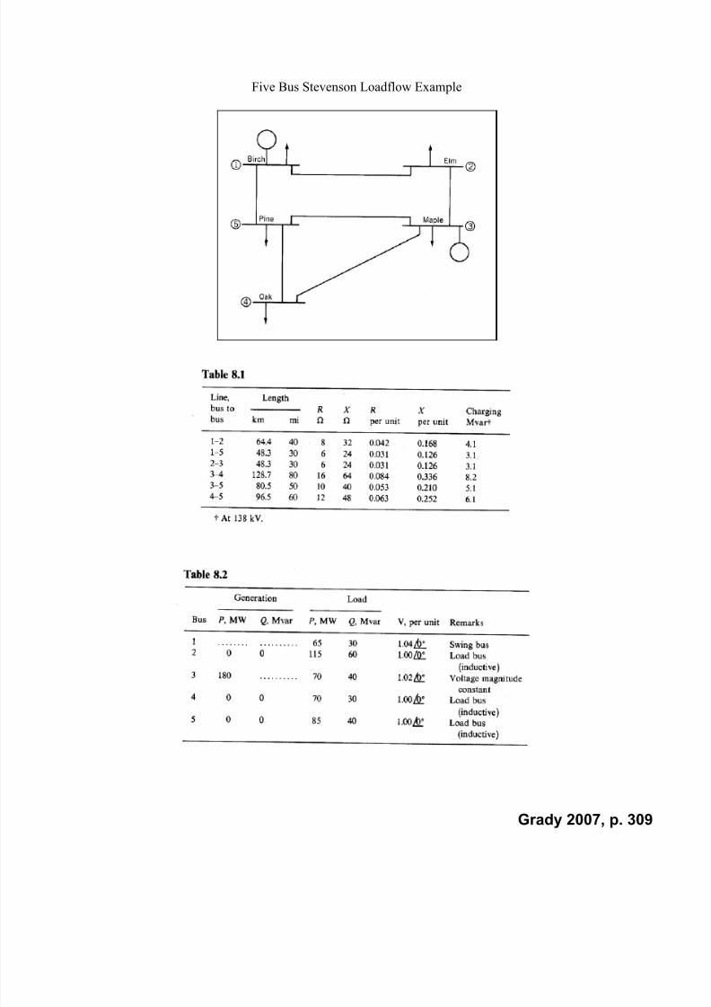
7/22/2019 Fundamentals Grady Notes June 2007 Print
http://slidepdf.com/reader/full/fundamentals-grady-notes-june-2007-print 309/388
Five Bus Stevenson Loadflow Example
Grady 2007, p. 309
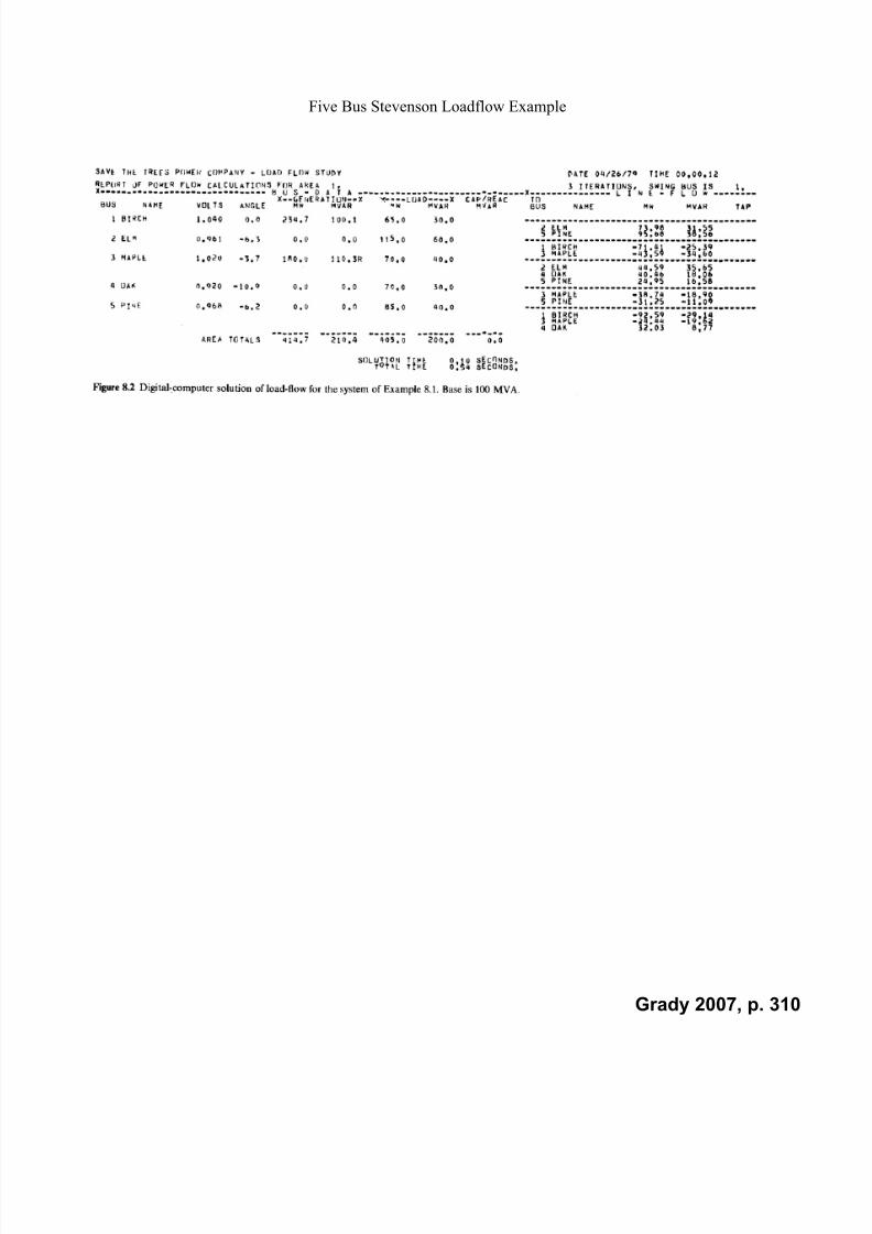
7/22/2019 Fundamentals Grady Notes June 2007 Print
http://slidepdf.com/reader/full/fundamentals-grady-notes-june-2007-print 310/388
Five Bus Stevenson Loadflow Example
Grady 2007, p. 310

7/22/2019 Fundamentals Grady Notes June 2007 Print
http://slidepdf.com/reader/full/fundamentals-grady-notes-june-2007-print 311/388
: F i v e
B u s
S t e v e n s o n
L o a
d f l o w
C a s e
: B u s
D a
t a
: :
L i n e
a r
L i n e a r
L i n e a r
L i n e a r
S h u n
t
M a x
i m u m
M i n i m u m
:
P
Q
P
Q
D e s
i r e d
R e a c
t i v e
Q
Q
B u s
R e m o
t e -
: B u s
B u s
B u s
G e n
e r a
t i o n
G e n e r a
t i o n
L o a
d
L o a
d
V o
l t a g e
Q L o a
d
G e n e r a
t i o n
G e n e r a
t i o n
C o n
t r o l
C o n
t r o l l e d
: N u m
b e r
N a m e
T y p e
( % )
( % )
( % )
( % )
( p u
)
( % )
( % )
( % )
A r e a
B u s
N o .
: ( I )
( A )
( I )
( F )
( F )
( F )
( F )
( F )
( F )
( F )
( F )
( I )
( I )
1 b i r c h
1
0
0
6 5
3 0
1 . 0
4
0
0
0
1
0
2 e
l m
3
0
0
1 1 5
6 0
0
0
0
0
1
0
3 m a p
l e
2
1 8 0
0
7 0
4 0
1 . 0
2
0
0
0
1
0
4 o a
k
3
0
0
7 0
3 0
0
0
0
0
1
0
5 p
i n e
3
0
0
8 5
4 0
0
0
0
0
1
0
: F i v e
B u s
S t e v e n s o n
L o a
d f l o w
C a s e
: L i n e a n
d T r a n s
f o r m e r
D a
t a
D e s
i r e d V o
l t a g e
:
a t V o
l t a g e
:
C o n
t . B u s
:
( p u
)
:
P o s
i t i v e
P o s
i t i v e
P o s
/ N e g
V o
l t a g e -
V o
l t a g e -
o r
D e s
i r e d P
:
S e q
u e n c e
S e q u e n c e
S e q u e n c e
M i n i m u m
M a x
i m u m
T a p
F i x e d
P h a s e
C o n
t .
C o n
t .
f o r
: F r o m
T o
C i r c u
i t
R
X
C h a r g
i n g
R a
t i n g
T a p
T a p
S t e p
S i z e
T a p
S h i f t
B u s
B u s
P h a s e
S h i f t e r
: B u s
B u s
N u m
b e r
( p u )
( p u
)
( % )
( % )
( p u
)
( p u
)
( p u
)
( p u )
( D e g r e e s
) N u m
b e r
S i d e
( % )
: ( I )
( I )
( I )
( F )
( F )
( F )
( F )
( F )
( F )
( F )
( F )
( F )
( I )
( I )
( F )
1
2
1
0 . 0
4 2
0 . 1
6 8
4 . 1
0
0
0
0
0
0
0
0
0
1
5
1
0 . 0
3 1
0 . 1
2 6
3 . 1
0
0
0
0
0
0
0
0
0
2
3
1
0 . 0
3 1
0 . 1
2 6
3 . 1
0
0
0
0
0
0
0
0
0
3
4
1
0 . 0
8 4
0 . 3
3 6
8 . 2
0
0
0
0
0
0
0
0
0
3
5
1
0 . 0
5 3
0 . 2
1
5 . 1
0
0
0
0
0
0
0
0
0
4
5
1
0 . 0
6 3
0 . 2
5 2
6 . 1
0
0
0
0
0
0
0
0
0
Grady 2007, p. 311

7/22/2019 Fundamentals Grady Notes June 2007 Print
http://slidepdf.com/reader/full/fundamentals-grady-notes-june-2007-print 312/388
Screwbean Wind Farm Study
Page 1 of 2
The Screwbean 138kV substation is located in west Texas, halfway between Midland/Odessa
and El Paso, near Guadalupe Mountains National Park. It is about 400 miles from Austin. Thisis prime wind country, and several wind farms are already located in the area.
Your job is to examine the feasibility of transporting 50MW of power from a new wind farm
near Screwbean to the U.T. Austin campus. In particular, you are to determine the impact of thistransaction on the losses in individual control areas, and also determine if any high or low
voltages, or line overloads, are created by your transaction.
To perform the analysis, you will use a 5000 bus version of PCFLO, together with a summer
peak loadflow case (in which most bus names have been disguised). You should prepare a ½ to
1 page summary report of your study, as if you were going to submit it to your client. Tablesshould be attached as an appendix.
Explain to your client how many MW must be generated at Screwbean to deliver 50MW to U.T.Austin. Quantify the MW needed by each negatively-impacted control area to pay back for their
increased losses.
Here are the steps:
1. Go to www.ece.utexas.edu/~grady, and click the PCFLO_V6 link. Follow the download and
unzip instructions on the PCFLO page.
2. The _SCREWBEAN case is your “base case.” Solve it using PCFLO_V6_Interface.exe.
Using Excel, examine the output files produced, notably
exlog_SCREWBEAN.csv
asoln_SCREWBEAN.csv
vsoln_SCREWBEAN.csv isoln_SCREWBEAN.csv and
out5_SCREWBEAN.csv.
3. Print out asoln_SCREWBEAN.csv, using the landscape option. To verify your loadflow
result, check your power loss in asoln_SCREWBEAN.csv. It should be about 1215 MW.
4. Find the Screwbean 138kV substation (SCRWBEAN 138, bus 1095) and the U.T. Austin
Harris 69kV substation (HARRIS 69, bus 9204) in the out5_SCREWBEAN.csv file. Notetheir voltage magnitudes and phase angles, and the P and Q flows in lines/transformers
attached to these busses.
5. Copy files bdat_SCREWBEAN.csv to bdat_mod, ldat_SCREWBEAN.csv to ldat_mod, and
adat_SCREWBEAN.csv to adat_mod.
6. Add new PV bus SB WIND as bus 2 to bdat_mod.csv, using 20 for its control area. Put50MW (i.e., 50% on 100MVA base) of generation on this new bus, with a Max Q Gen of
25MVAr, and a Min Q Gen of negative 12.5MVAr. For the desired voltage, put a value that
is 0.005pu higher than the base case voltage at SCRWBEAN 138.
Grady 2007, p. 312

7/22/2019 Fundamentals Grady Notes June 2007 Print
http://slidepdf.com/reader/full/fundamentals-grady-notes-june-2007-print 313/388
Screwbean Wind Farm Study
Page 2 of 2
7. Add new PQ bus UT CAMPUS as bus 3 to bdat_mod.csv, using 21 for its control area. Put50MW, 25MVAr of load on this new bus.
8. Connect new bus SB WIND to SCRWBEAN 138 through a line with impedance R =
0.001pu, X = 0.01pu, B = 0%.
9. Connect new bus UT CAMPUS to HARRIS 69 through a line with impedance R = 0.001pu,
X = 0.01pu, B = 0%.
10. Add control area SB as area 20 to adat_mod.csv, with a desired export of 50MW (i.e., 50%).
The area control bus number will be that of SB WIND. Use an export solution tolerance of0.1%.
11. Add control area UT as area 21 to adat_mod.csv, with a desired import of 50MW (i.e.,negative 50MW export). The area control bus number will be that of UT CAMPUS. Use an
export solution tolerance of 0.1%.
12. Re-run PCFLO_V6_Interface.exe, using _mod as the input case. Print out the new asoln.csv
file (using the landscape option), and using the new asoln file, tabulate area by area the
increase/decrease in each control area’s losses compared to the base case. The areas with
increased losses may reasonably expect MW payment from the wind power company. Thiscan be accomplished by putting in generator larger than 50MW, and exporting some power
to the control areas that are negatively impacted.
13. Use the loss increases from Step 12 to estimate how much actual generation would be needed
at SB WIND to deliver 50MW to UT CAMPUS and payback the extra losses to thenegatively-impacted control areas.
14. Check for any line overloads and high/low voltages created in the vicinity of SCRWBEAN138 and HARRIS 69. (In an actual study, there would have to be described and remedies
proposed. However, do not investigate remedies in your study.)
15. Repeat the above process, but this time reverse the transaction by putting a wind generator at
UT CAMPUS, and a 50MW load at SB WIND.
16. Describe the impacts of both transactions in your report.
Grady 2007, p. 313

7/22/2019 Fundamentals Grady Notes June 2007 Print
http://slidepdf.com/reader/full/fundamentals-grady-notes-june-2007-print 314/388
Grady 2007, p. 314

7/22/2019 Fundamentals Grady Notes June 2007 Print
http://slidepdf.com/reader/full/fundamentals-grady-notes-june-2007-print 315/388
Grady 2007, p. 315

7/22/2019 Fundamentals Grady Notes June 2007 Print
http://slidepdf.com/reader/full/fundamentals-grady-notes-june-2007-print 316/388
Grady 2007, p. 316

7/22/2019 Fundamentals Grady Notes June 2007 Print
http://slidepdf.com/reader/full/fundamentals-grady-notes-june-2007-print 317/388
Grady 2007, p. 317
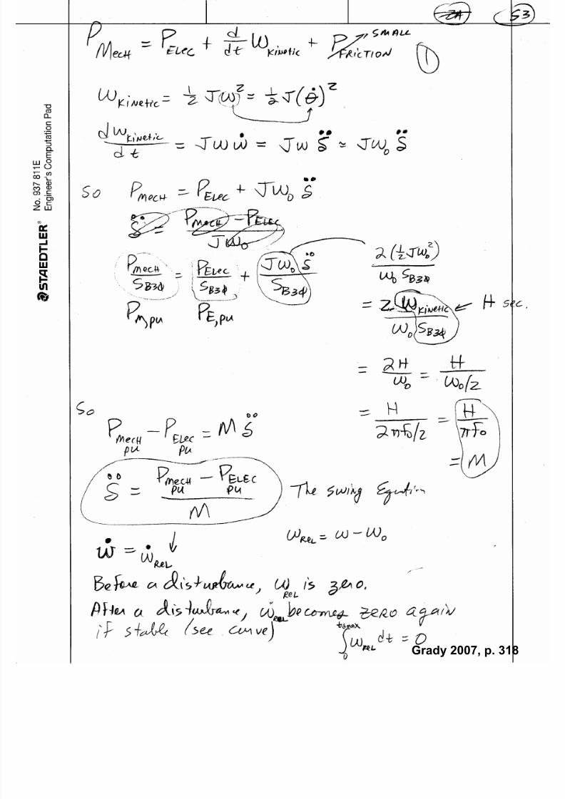
7/22/2019 Fundamentals Grady Notes June 2007 Print
http://slidepdf.com/reader/full/fundamentals-grady-notes-june-2007-print 318/388
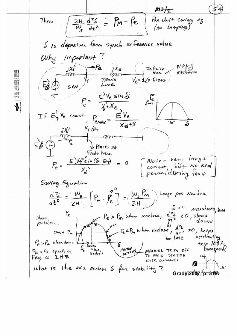
7/22/2019 Fundamentals Grady Notes June 2007 Print
http://slidepdf.com/reader/full/fundamentals-grady-notes-june-2007-print 319/388
Grady 2007, p. 319

7/22/2019 Fundamentals Grady Notes June 2007 Print
http://slidepdf.com/reader/full/fundamentals-grady-notes-june-2007-print 320/388
Grady 2007, p. 320
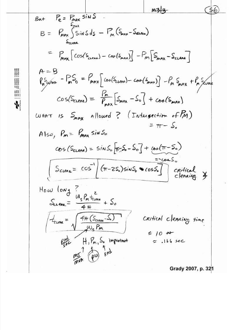
7/22/2019 Fundamentals Grady Notes June 2007 Print
http://slidepdf.com/reader/full/fundamentals-grady-notes-june-2007-print 321/388
Grady 2007, p. 321

7/22/2019 Fundamentals Grady Notes June 2007 Print
http://slidepdf.com/reader/full/fundamentals-grady-notes-june-2007-print 322/388
Grady 2007, p. 322

7/22/2019 Fundamentals Grady Notes June 2007 Print
http://slidepdf.com/reader/full/fundamentals-grady-notes-june-2007-print 323/388
Grady 2007, p. 323

7/22/2019 Fundamentals Grady Notes June 2007 Print
http://slidepdf.com/reader/full/fundamentals-grady-notes-june-2007-print 324/388
Grady 2007, p. 324

7/22/2019 Fundamentals Grady Notes June 2007 Print
http://slidepdf.com/reader/full/fundamentals-grady-notes-june-2007-print 325/388
Grady 2007, p. 325
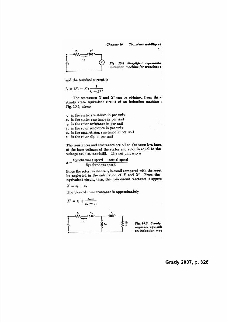
7/22/2019 Fundamentals Grady Notes June 2007 Print
http://slidepdf.com/reader/full/fundamentals-grady-notes-june-2007-print 326/388
Grady 2007, p. 326

7/22/2019 Fundamentals Grady Notes June 2007 Print
http://slidepdf.com/reader/full/fundamentals-grady-notes-june-2007-print 327/388
Steady State Model for Round Rotor Machine
Va and Ia are the terminal voltage and current. Xs is the synchronous reactance. Resistance r is
the stator resistance. Ea is the Thevenin equivalent voltage behind synchronous reactance.
Steady-State Model for Salient Pole Machine
(No equivalent circuit. Phasor diagram only)
Steps when Va and Ia are known:
With Va, Ia, r, and Xq, find phasor a’ to locate the q-axis.
Then, compute Ia projections Iaq and Iad where
Iaq has magnitude aa I I cos and has phase angle ,
Iad has magnitude aa I I sin and has phase angle 90 ,
and where a I is the angle of Ia.
Then, find Ea.
+
Ea
–
+
Va
–
jXs r
Ia
Ea
jXsIa
rIa
Va
Ia
q-axis
d-axis
reference
Ea
jXqIa
rIa
Va
Ia
q-axis
d-axis
reference
Iaq
Iad jXdIad
jXqIaq
a’
Grady 2007, p. 327

7/22/2019 Fundamentals Grady Notes June 2007 Print
http://slidepdf.com/reader/full/fundamentals-grady-notes-june-2007-print 328/388
Transient Stability Machine Model 1
Constant Voltage Magnitude E’ Behind Transient Reactance Xd’
This model is like the round rotor synchronous model, except that the transient reactance is used
instead of the synchronous reactance.
Transient Stability Machine Model 2
Salient Pole Rotor
Steps when Va and Ia are known: Begin with same steps used in the salient pole synchronous
machine model. Then, use Xd’ and Iad to find Ea’.
The magnitude of Ea’ varies according to a fd
do
a E E
T dt
E d
'
'1
, where Tdo’ is the direct-
axis transient open circuit time constant, and Efd is the field voltage (as seen from the stator). As
a first approximation, Efd is treated as a constant whose initial value is the same as the initial
value of a E .
+
E’
–
+
Va
–
jXd’ r
Ia
E’
j Xd’Ia
rIa
Va
Ia
q-axis
d-axis
reference
Ea
jXqIa
rIa
Va
Ia
q-axis
d-axis
reference
Iaq
Iad jXdIad
jXqIaq
a’
jXd’ Iad
Ea’
Grady 2007, p. 328

7/22/2019 Fundamentals Grady Notes June 2007 Print
http://slidepdf.com/reader/full/fundamentals-grady-notes-june-2007-print 329/388
A synchronous generator is operating in steady-state with the following conditions (in per unit):
Va = 1.0/0°, Ia = 0.8/-30°, Xd = 1.0, Xq = 0.6, r = 0. Find S (at the machine terminals), and
phasors Iad, Iaq, Ea.
Grady 2007, p. 329

7/22/2019 Fundamentals Grady Notes June 2007 Print
http://slidepdf.com/reader/full/fundamentals-grady-notes-june-2007-print 330/388
Grady 2007, p. 330
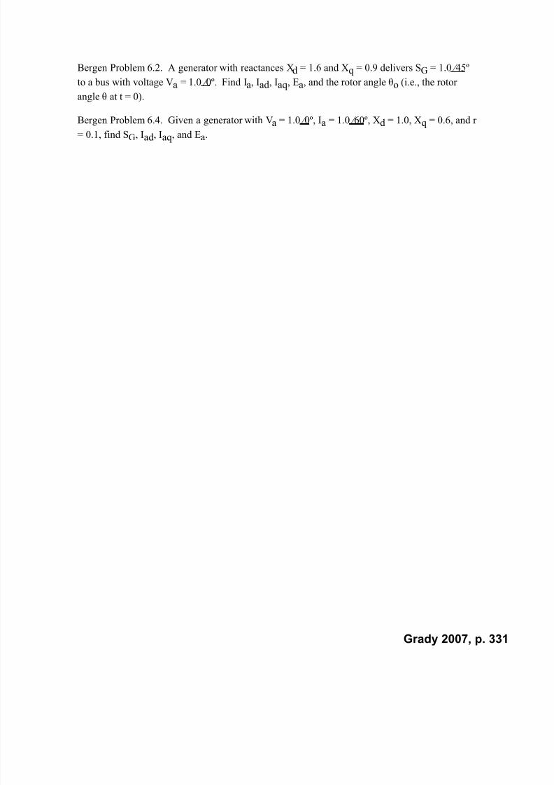
7/22/2019 Fundamentals Grady Notes June 2007 Print
http://slidepdf.com/reader/full/fundamentals-grady-notes-june-2007-print 331/388
Bergen Problem 6.2. A generator with reactances Xd = 1.6 and Xq = 0.9 delivers SG = 1.0 ⁄45º
to a bus with voltage Va = 1.0 ⁄0º. Find Ia, Iad, Iaq, Ea, and the rotor angle o (i.e., the rotor
angle at t = 0).
Bergen Problem 6.4. Given a generator with Va = 1.0 ⁄0º, Ia = 1.0 ⁄60º, Xd = 1.0, Xq = 0.6, and r
= 0.1, find SG, Iad, Iaq, and Ea.
Grady 2007, p. 331

7/22/2019 Fundamentals Grady Notes June 2007 Print
http://slidepdf.com/reader/full/fundamentals-grady-notes-june-2007-print 332/388
Grady 2007, p. 332

7/22/2019 Fundamentals Grady Notes June 2007 Print
http://slidepdf.com/reader/full/fundamentals-grady-notes-june-2007-print 333/388
Grady 2007, p. 333

7/22/2019 Fundamentals Grady Notes June 2007 Print
http://slidepdf.com/reader/full/fundamentals-grady-notes-june-2007-print 334/388
A new 32MVA, 60Hz steam generator was recently installed at the UT power plant. The
generator is connected through a large reactor to ERCOT at the Harris 12kV bus.
The electrical diagram and internal voltage (for the transient condition) that exists when the
generator is producing (25MW + j12.4MVAr) is shown below. Suddenly, at t = 0, a three-phase
fault with zero impedance occurs at the Harris 12kV bus. Assuming that E’, Vth, and Pmech are
constant, determine the critical clearing time (in cycles). Use the attached graph to show
important P and points and lines on the power curve, and show clearly which areas are equal.
Remember that during the fault, the electrical power output is zero, and thus the rotor accelerates
according to omech s t
H
P t
2
4)( , where )0( t o . Also, note that s =
377rad/sec, is in radians, and mech P is in pu. The formula for critical clearing angle is
)cos()sin()2(cos 1ooocrit .
E’/°
jXd’ jXr jXth
Vth/0°
Harris 12kV bus
Machine E’ = 1.100pu
Machine = 16.5°Machine P = 25MW (i.e., 0.781pu)
Machine jXd’ = j0.22pu
Machine H = 1.4seconds
Reactor jXr = j0.17pu
Thevenin jXth = j0.01pu
Thevenin Vth = (1.0 + j0)pu
Values given on the generator base
Grady 2007, p. 334

7/22/2019 Fundamentals Grady Notes June 2007 Print
http://slidepdf.com/reader/full/fundamentals-grady-notes-june-2007-print 335/388
0
0.5
1
1.5
2
2.5
3
3.5
4
0 30 60 90 120 150 180
Grady 2007, p. 335

7/22/2019 Fundamentals Grady Notes June 2007 Print
http://slidepdf.com/reader/full/fundamentals-grady-notes-june-2007-print 336/388
Grady 2007, p. 336

7/22/2019 Fundamentals Grady Notes June 2007 Print
http://slidepdf.com/reader/full/fundamentals-grady-notes-june-2007-print 337/388
Grady 2007, p. 337

7/22/2019 Fundamentals Grady Notes June 2007 Print
http://slidepdf.com/reader/full/fundamentals-grady-notes-june-2007-print 338/388
Grady 2007, p. 338

7/22/2019 Fundamentals Grady Notes June 2007 Print
http://slidepdf.com/reader/full/fundamentals-grady-notes-june-2007-print 339/388
Grady 2007, p. 339
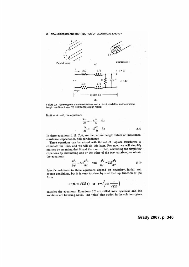
7/22/2019 Fundamentals Grady Notes June 2007 Print
http://slidepdf.com/reader/full/fundamentals-grady-notes-june-2007-print 340/388
Grady 2007, p. 340

7/22/2019 Fundamentals Grady Notes June 2007 Print
http://slidepdf.com/reader/full/fundamentals-grady-notes-june-2007-print 341/388
Grady 2007, p. 341
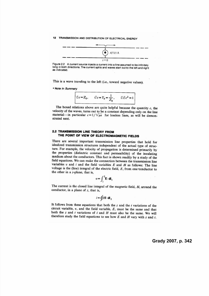
7/22/2019 Fundamentals Grady Notes June 2007 Print
http://slidepdf.com/reader/full/fundamentals-grady-notes-june-2007-print 342/388
Grady 2007, p. 342

7/22/2019 Fundamentals Grady Notes June 2007 Print
http://slidepdf.com/reader/full/fundamentals-grady-notes-june-2007-print 343/388
Grady 2007, p. 343

7/22/2019 Fundamentals Grady Notes June 2007 Print
http://slidepdf.com/reader/full/fundamentals-grady-notes-june-2007-print 344/388
Grady 2007, p. 344

7/22/2019 Fundamentals Grady Notes June 2007 Print
http://slidepdf.com/reader/full/fundamentals-grady-notes-june-2007-print 345/388
Grady 2007, p. 345

7/22/2019 Fundamentals Grady Notes June 2007 Print
http://slidepdf.com/reader/full/fundamentals-grady-notes-june-2007-print 346/388
Grady 2007, p. 346

7/22/2019 Fundamentals Grady Notes June 2007 Print
http://slidepdf.com/reader/full/fundamentals-grady-notes-june-2007-print 347/388
Grady 2007, p. 347

7/22/2019 Fundamentals Grady Notes June 2007 Print
http://slidepdf.com/reader/full/fundamentals-grady-notes-june-2007-print 348/388
Grady 2007, p. 348

7/22/2019 Fundamentals Grady Notes June 2007 Print
http://slidepdf.com/reader/full/fundamentals-grady-notes-june-2007-print 349/388
Grady 2007, p. 349

7/22/2019 Fundamentals Grady Notes June 2007 Print
http://slidepdf.com/reader/full/fundamentals-grady-notes-june-2007-print 350/388
Grady 2007, p. 350

7/22/2019 Fundamentals Grady Notes June 2007 Print
http://slidepdf.com/reader/full/fundamentals-grady-notes-june-2007-print 351/388
Grady 2007, p. 351
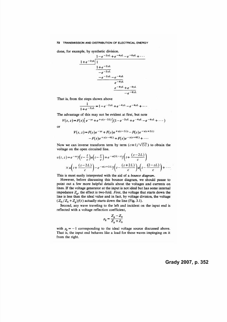
7/22/2019 Fundamentals Grady Notes June 2007 Print
http://slidepdf.com/reader/full/fundamentals-grady-notes-june-2007-print 352/388
Grady 2007, p. 352

7/22/2019 Fundamentals Grady Notes June 2007 Print
http://slidepdf.com/reader/full/fundamentals-grady-notes-june-2007-print 353/388
Grady 2007, p. 353

7/22/2019 Fundamentals Grady Notes June 2007 Print
http://slidepdf.com/reader/full/fundamentals-grady-notes-june-2007-print 354/388
Grady 2007, p. 354

7/22/2019 Fundamentals Grady Notes June 2007 Print
http://slidepdf.com/reader/full/fundamentals-grady-notes-june-2007-print 355/388
Grady 2007, p. 355

7/22/2019 Fundamentals Grady Notes June 2007 Print
http://slidepdf.com/reader/full/fundamentals-grady-notes-june-2007-print 356/388
Grady 2007, p. 356

7/22/2019 Fundamentals Grady Notes June 2007 Print
http://slidepdf.com/reader/full/fundamentals-grady-notes-june-2007-print 357/388
Grady 2007, p. 357

7/22/2019 Fundamentals Grady Notes June 2007 Print
http://slidepdf.com/reader/full/fundamentals-grady-notes-june-2007-print 358/388
Grady 2007, p. 358

7/22/2019 Fundamentals Grady Notes June 2007 Print
http://slidepdf.com/reader/full/fundamentals-grady-notes-june-2007-print 359/388
Grady 2007, p. 359

7/22/2019 Fundamentals Grady Notes June 2007 Print
http://slidepdf.com/reader/full/fundamentals-grady-notes-june-2007-print 360/388
Grady 2007, p. 360

7/22/2019 Fundamentals Grady Notes June 2007 Print
http://slidepdf.com/reader/full/fundamentals-grady-notes-june-2007-print 361/388
Grady 2007, p. 361
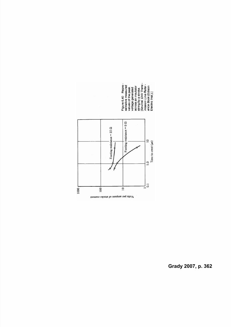
7/22/2019 Fundamentals Grady Notes June 2007 Print
http://slidepdf.com/reader/full/fundamentals-grady-notes-june-2007-print 362/388
Grady 2007, p. 362
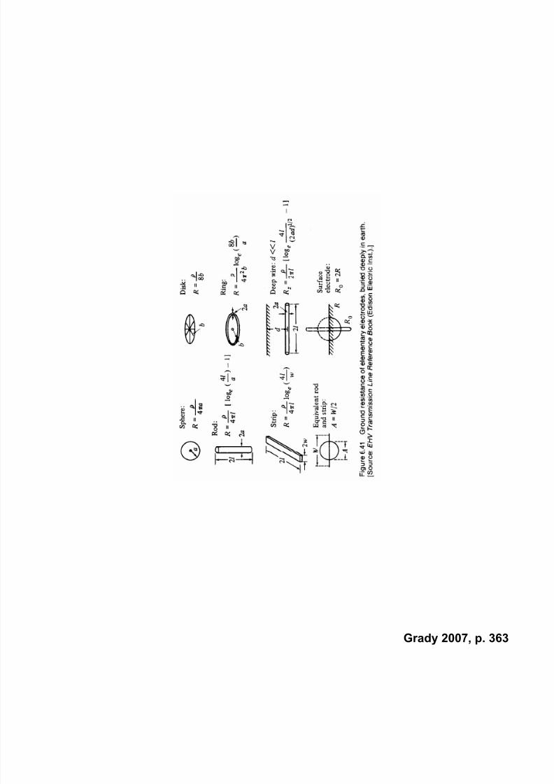
7/22/2019 Fundamentals Grady Notes June 2007 Print
http://slidepdf.com/reader/full/fundamentals-grady-notes-june-2007-print 363/388
Grady 2007, p. 363
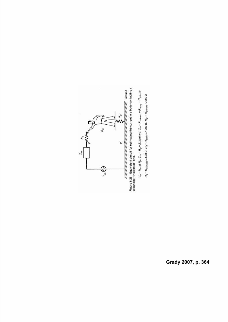
7/22/2019 Fundamentals Grady Notes June 2007 Print
http://slidepdf.com/reader/full/fundamentals-grady-notes-june-2007-print 364/388
Grady 2007, p. 364

7/22/2019 Fundamentals Grady Notes June 2007 Print
http://slidepdf.com/reader/full/fundamentals-grady-notes-june-2007-print 365/388
Grady 2007, p. 365

7/22/2019 Fundamentals Grady Notes June 2007 Print
http://slidepdf.com/reader/full/fundamentals-grady-notes-june-2007-print 366/388
Grady 2007, p. 366
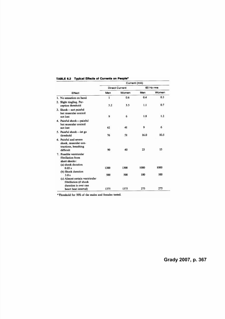
7/22/2019 Fundamentals Grady Notes June 2007 Print
http://slidepdf.com/reader/full/fundamentals-grady-notes-june-2007-print 367/388
Grady 2007, p. 367
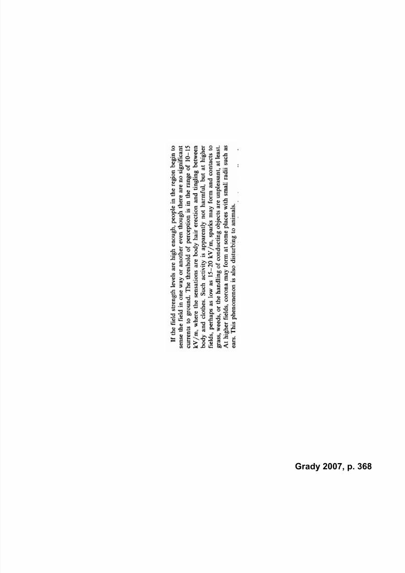
7/22/2019 Fundamentals Grady Notes June 2007 Print
http://slidepdf.com/reader/full/fundamentals-grady-notes-june-2007-print 368/388
Grady 2007, p. 368
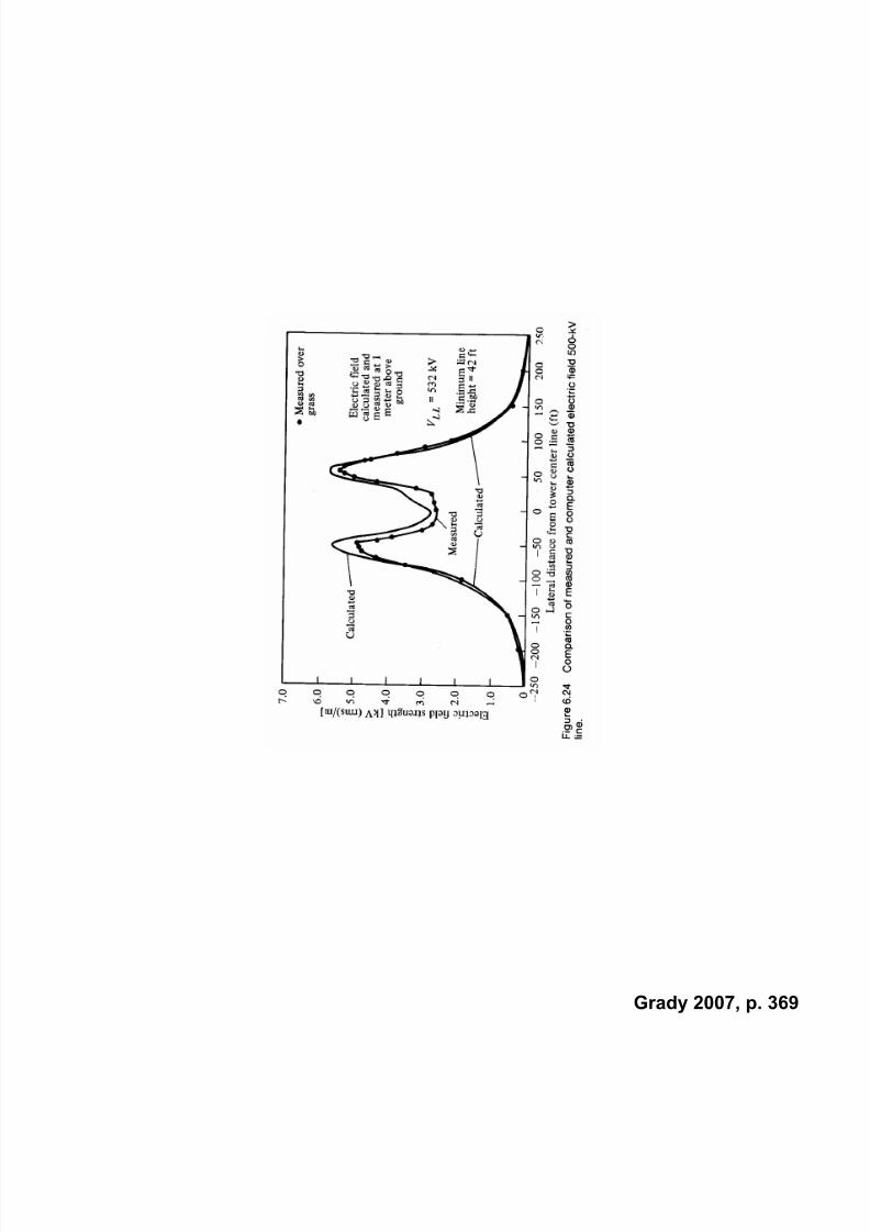
7/22/2019 Fundamentals Grady Notes June 2007 Print
http://slidepdf.com/reader/full/fundamentals-grady-notes-june-2007-print 369/388
Grady 2007, p. 369

7/22/2019 Fundamentals Grady Notes June 2007 Print
http://slidepdf.com/reader/full/fundamentals-grady-notes-june-2007-print 370/388
Grady 2007, p. 370
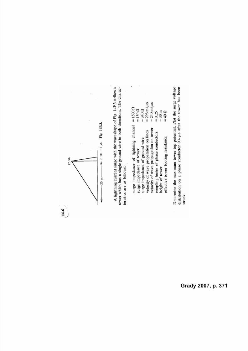
7/22/2019 Fundamentals Grady Notes June 2007 Print
http://slidepdf.com/reader/full/fundamentals-grady-notes-june-2007-print 371/388
Grady 2007, p. 371
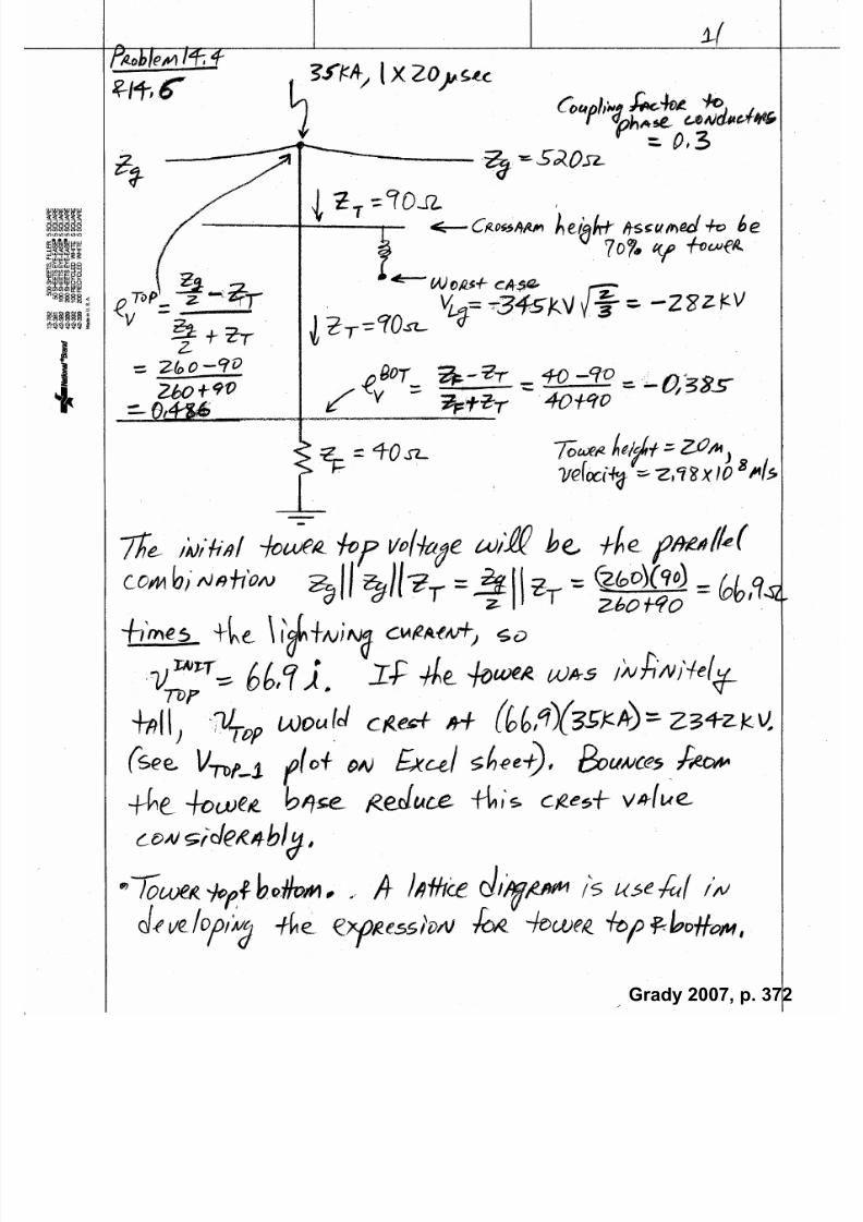
7/22/2019 Fundamentals Grady Notes June 2007 Print
http://slidepdf.com/reader/full/fundamentals-grady-notes-june-2007-print 372/388
Grady 2007, p. 372
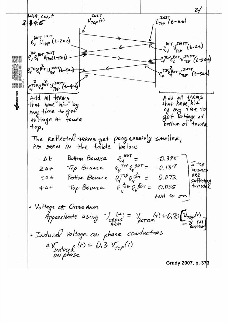
7/22/2019 Fundamentals Grady Notes June 2007 Print
http://slidepdf.com/reader/full/fundamentals-grady-notes-june-2007-print 373/388
Grady 2007, p. 373

7/22/2019 Fundamentals Grady Notes June 2007 Print
http://slidepdf.com/reader/full/fundamentals-grady-notes-june-2007-print 374/388
Grady 2007, p. 374

7/22/2019 Fundamentals Grady Notes June 2007 Print
http://slidepdf.com/reader/full/fundamentals-grady-notes-june-2007-print 375/388
Grady 2007, p. 375

7/22/2019 Fundamentals Grady Notes June 2007 Print
http://slidepdf.com/reader/full/fundamentals-grady-notes-june-2007-print 376/388
Grady 2007, p. 376
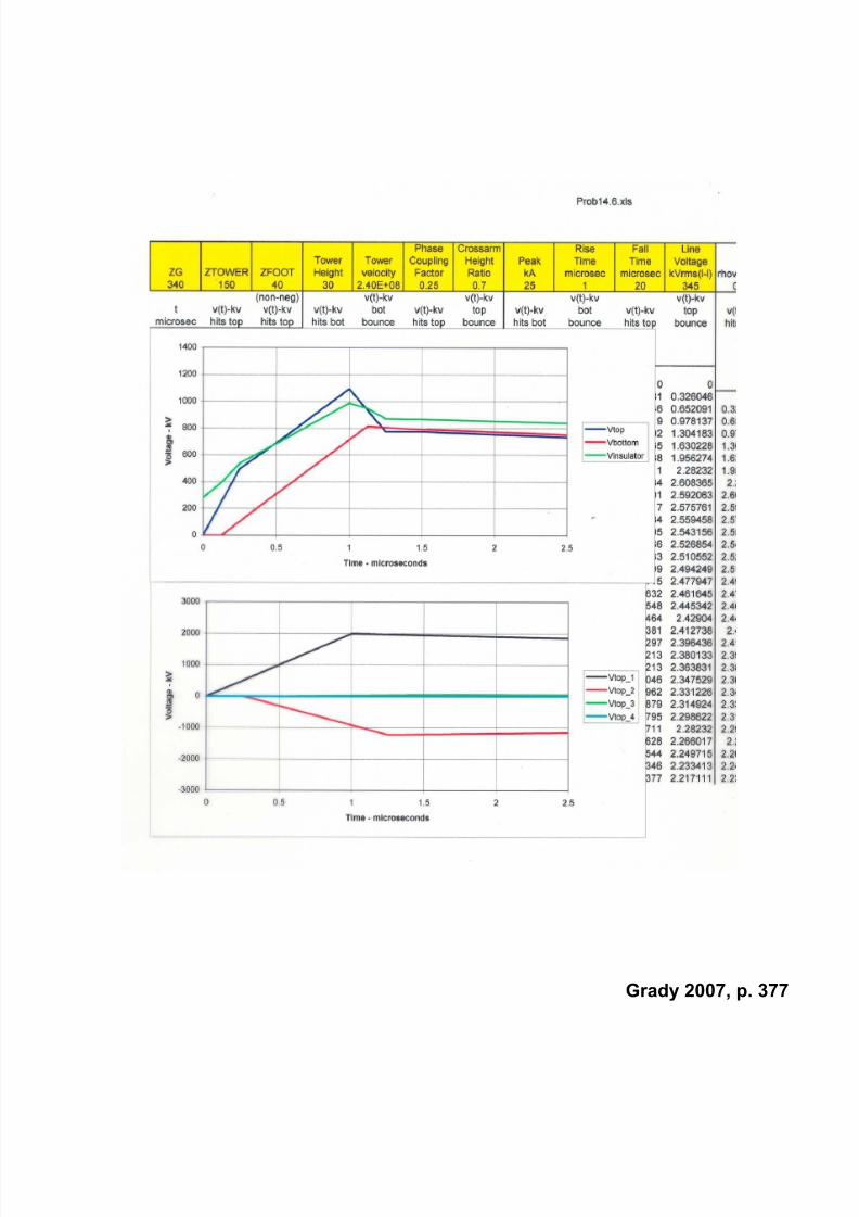
7/22/2019 Fundamentals Grady Notes June 2007 Print
http://slidepdf.com/reader/full/fundamentals-grady-notes-june-2007-print 377/388
Grady 2007, p. 377

7/22/2019 Fundamentals Grady Notes June 2007 Print
http://slidepdf.com/reader/full/fundamentals-grady-notes-june-2007-print 378/388
Grady 2007, p. 378

7/22/2019 Fundamentals Grady Notes June 2007 Print
http://slidepdf.com/reader/full/fundamentals-grady-notes-june-2007-print 379/388
Grady 2007, p. 379

7/22/2019 Fundamentals Grady Notes June 2007 Print
http://slidepdf.com/reader/full/fundamentals-grady-notes-june-2007-print 380/388
Grady 2007, p. 380
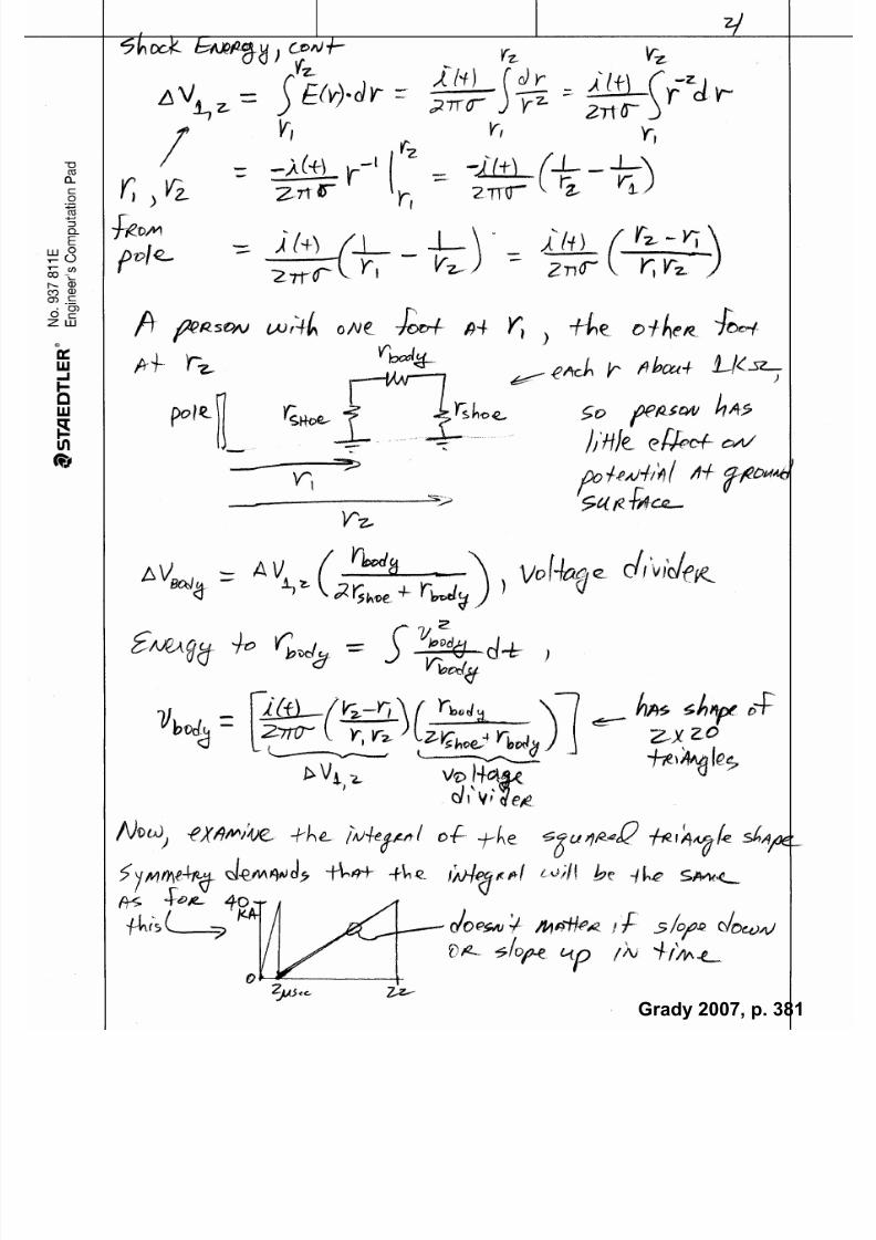
7/22/2019 Fundamentals Grady Notes June 2007 Print
http://slidepdf.com/reader/full/fundamentals-grady-notes-june-2007-print 381/388

7/22/2019 Fundamentals Grady Notes June 2007 Print
http://slidepdf.com/reader/full/fundamentals-grady-notes-june-2007-print 382/388
Grady 2007, p. 382
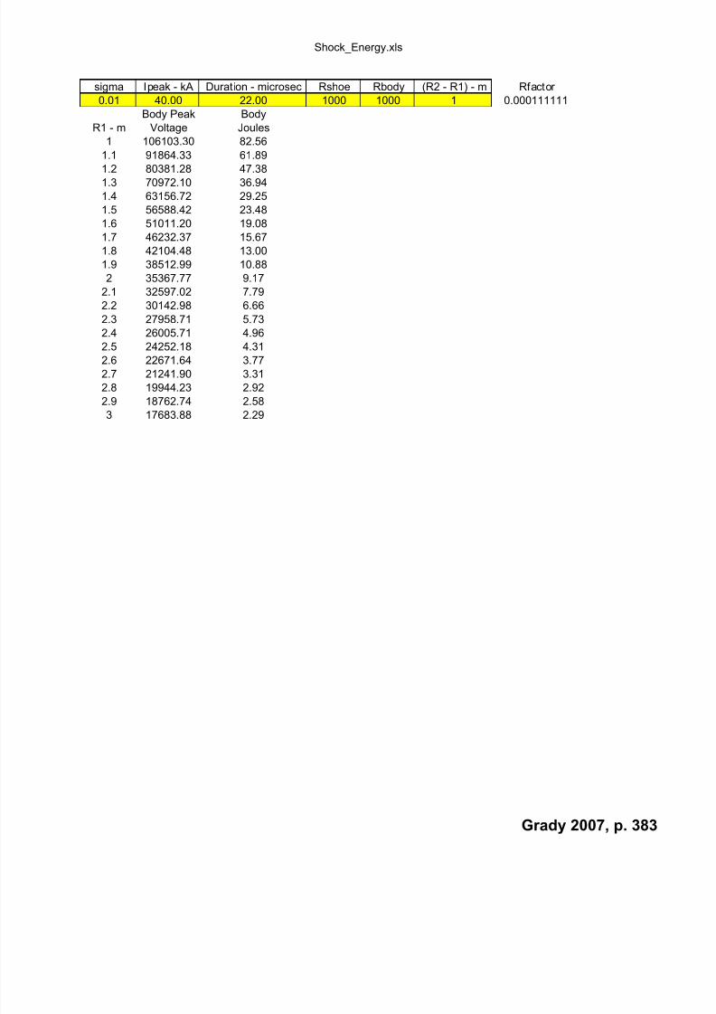
7/22/2019 Fundamentals Grady Notes June 2007 Print
http://slidepdf.com/reader/full/fundamentals-grady-notes-june-2007-print 383/388
Shock_Energy.xls
sigma Ipeak - kA Duration - microsec Rshoe Rbody (R2 - R1) - m Rfactor
0.01 40.00 22.00 1000 1000 1 0.000111111
Body Peak Body
R1 - m Voltage Joules
1 106103.30 82.56
1.1 91864.33 61.89
1.2 80381.28 47.381.3 70972.10 36.94
1.4 63156.72 29.25
1.5 56588.42 23.48
1.6 51011.20 19.08
1.7 46232.37 15.67
1.8 42104.48 13.00
1.9 38512.99 10.88
2 35367.77 9.17
2.1 32597.02 7.79
2.2 30142.98 6.66
2.3 27958.71 5.73
2.4 26005.71 4.962.5 24252.18 4.31
2.6 22671.64 3.77
2.7 21241.90 3.31
2.8 19944.23 2.92
2.9 18762.74 2.58
3 17683.88 2.29
Grady 2007, p. 383

7/22/2019 Fundamentals Grady Notes June 2007 Print
http://slidepdf.com/reader/full/fundamentals-grady-notes-june-2007-print 384/388
Shock_Energy.xls
sigma Ipeak - kA Duration - microsec Rshoe Rbody (R2 - R1) - m Rfactor
0.001 40.00 22.00 1000 1000 1 0.000111111
Body Peak Body
R1 - m Voltage Joules
1 1061032.95 8255.80
2 353677.65 917.31
3 176838.83 229.334 106103.30 82.56
5 70735.53 36.69
6 50525.38 18.72
7 37894.03 10.53
8 29473.14 6.37
9 23578.51 4.08
10 19291.51 2.73
11 16076.26 1.90
12 13602.99 1.36
13 11659.70 1.00
14 10105.08 0.75
15 8841.94 0.5716 7801.71 0.45
17 6934.86 0.35
18 6204.87 0.28
19 5584.38 0.23
20 5052.54 0.19
21 4593.22 0.15
Grady 2007, p. 384

7/22/2019 Fundamentals Grady Notes June 2007 Print
http://slidepdf.com/reader/full/fundamentals-grady-notes-june-2007-print 385/388
Grady 2007, p. 385

7/22/2019 Fundamentals Grady Notes June 2007 Print
http://slidepdf.com/reader/full/fundamentals-grady-notes-june-2007-print 386/388
Grady 2007, p. 386
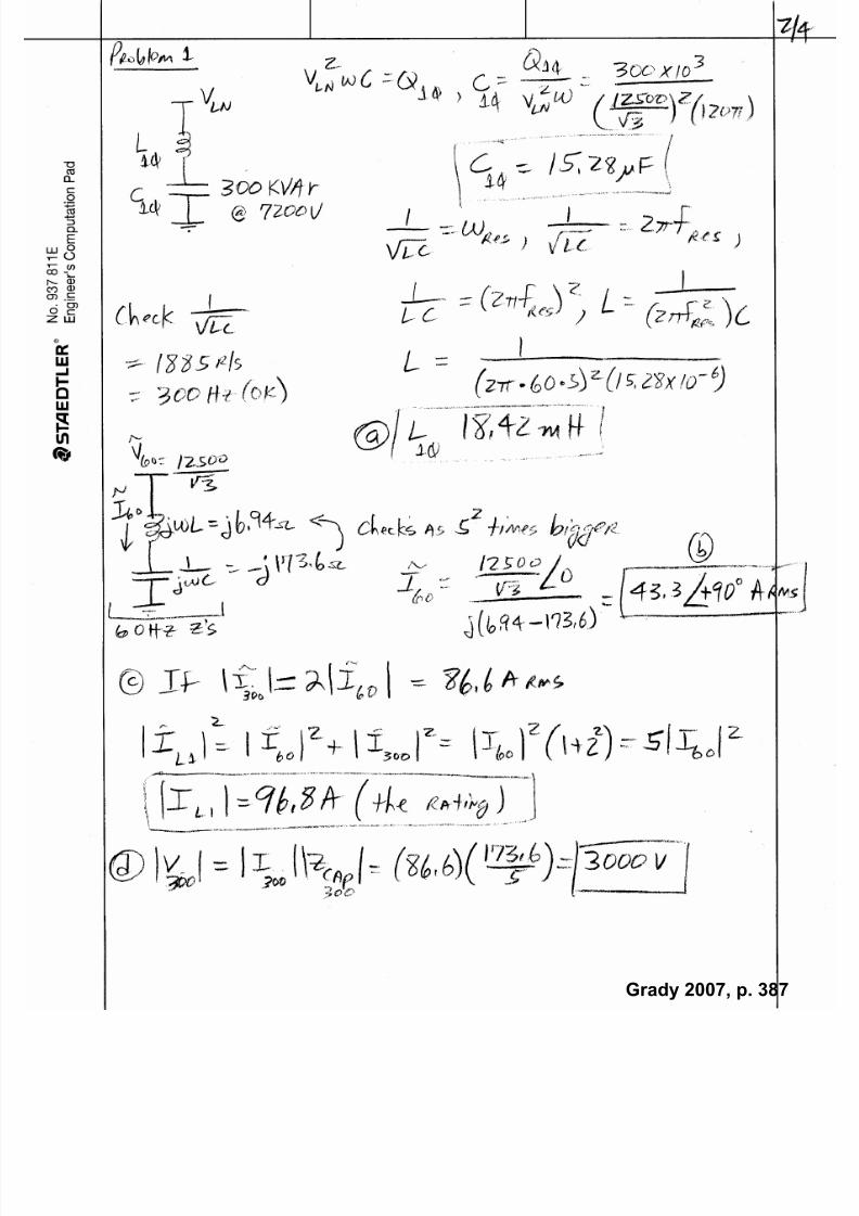
7/22/2019 Fundamentals Grady Notes June 2007 Print
http://slidepdf.com/reader/full/fundamentals-grady-notes-june-2007-print 387/388
Grady 2007, p. 387

7/22/2019 Fundamentals Grady Notes June 2007 Print
http://slidepdf.com/reader/full/fundamentals-grady-notes-june-2007-print 388/388