fundamental aspects of droplet combustion modelling

Shah Shahood Alam et al Int. Journal of Engineering Research and Applications www.ijera.com

ISSN : 2248-9622, Vol. 4, Issue 11(Version 3), November 2014, pp.10-26

www.ijera.com 10 |

P a g e

Fundamental Aspects of Droplet Combustion Modelling

Shah Shahood Alam*, Ahtisham A. Nizami, Tariq Aziz *Corresponding author. Address: Pollution and Combustion Engineering Lab. Department of Mechanical

Engineering. Aligarh Muslim University, Aligarh-202002, U.P. India.

ABSTRACT The present paper deals with important aspects of liquid droplet evaporation and combustion. A detailed

spherically symmetric, single component droplet combustion model is evolved first by solving time dependent

energy and species conservation equations in the gas phase using finite difference technique. Results indicate

that the flame diameter F first increases and then decreases and the square of droplet diameter decreases

linearly with time. Also, the /F D ratio increases throughout the droplet burning period unlike the quasi-steady

model where it assumes a large constant value. The spherically symmetric model is then extended to include the

effects of forced convection. Plots of 2D and droplet mass burning rate fm versus time are obtained for steady

state, droplet heating and heating with convection cases for a n-octane droplet of 1.3 mm diameter burning in

standard atmosphere. It is observed that the mass burning rate is highest for forced convective case and lowest

for droplet heating case. The corresponding values of droplet lifetime follow the inverse relationship with the

mass burning rate as expected. Emission data for a spherically symmetric, 100 m n-heptane droplet burning

in air are determined using the present gas phase model in conjunction with the Olikara and Borman code [1]

with the aim of providing a qualitative trend rather than quantitative with a simplified approach. It is observed

that the products of combustion maximise in the reaction zone and NO concentration is very sensitive to the

flame temperature. This paper also discusses the general methodology and basic governing equations for

analysing multicomponent and high pressure droplet vaporisation/combustion in a comprehensible manner. The

results of the present study compare fairly well with the experimental/theoretical observations of other authors

for the same conditions. The droplet sub models developed in the present work are accurate and yet simple for

their incorporation in spray combustion codes.

Keywords: droplet combustion models, gas and liquid phases, numerical solution, simplified approach, spray

combustion codes.

I. Introduction Combustion of liquid fuels provide a major

portion of world energy supply. In most of the

practical combustion devices like diesel engines, gas

turbines, industrial boilers and furnaces, liquid

rockets, liquid fuel is mixed with the oxidiser and

burned in the form of liquid sprays (made up of

discrete droplets). A spray may be regarded as a

turbulent, chemically reacting, multicomponent

(MC) flow with phase change involving

thermodynamics, heat and mass transport, chemical

kinetics and fluid dynamics.

Further, the submillimeter scales associated with

spray problem have made detailed experimental

measurements quite difficult. Hence in general,

theory and computations have led experiments in

analysing spray systems [2] with the aim to establish

design criteria for efficient combustors from

combustion and emission point of view.

Since direct studies on spray combustion may be

tedious and inaccurate, an essential pre-requisite for

understanding spray phenomenon is the knowledge

of the laws governing droplet evaporation and

combustion with the main objective of developing

computer models to give a better understanding of

spray combustion phenomenon. However, the

droplet models should be realistic and not too

complicated, so that they can be successfully

employed in spray codes, where CPU economy plays

a vital role [2].

An isolated droplet combustion under

microgravity (near zero gravity) condition is an ideal

situation for studying liquid droplet combustion

phenomenon. It leads to a simplified, one

dimensional solution approach of the droplet

combustion problem.

The resulting model is called „spherico-

symmetric droplet combustion model‟ (a spherical

liquid fuel droplet surrounded by a concentric,

spherically symmetric flame, with no relative

velocity between the droplet surface and surrounding

gas, that is, gas phase Reynolds number based on

droplet diameter gRe = 0).

Droplet combustion models available in the

literature are of varied nature. Most simplified

RESEARCH ARTICLE OPEN ACCESS


ISSN : 2248-9622, Vol. 4, Issue 11( Part 3), November 2014, pp.

www.ijera.com 11 | P a g e

models assume quasi-steadiness in both liquid

droplet and the surrounding gas phase.

In the quasi-steady liquid phase model, the

liquid droplet is at its boiling point temperature

evaporating steadily with a fixed diameter

surrounded by a concentric stationary flame, such

that the /F D ratio, also known as flame standoff

ratio assumes a constant value.

The justification of this assumption is based on

the relatively slow regression rate of the liquid fuel

droplet as compared to gas phase transport processes.

For the combustion of single component liquid

droplets or light distillate fuel oils in high

temperature ambient gas atmosphere, it is quite

accurate to assume that the droplet is at its boiling

point temperature sT = bT [3], (i.e. no droplet

heating or no need for solving the unsteady energy

equation within the liquid phase). The droplet

evaporates steadily following the 2d law (square

of instantaneous droplet diameter varying linearly

with time).

This quasi-steady liquid phase can be coupled

with a steady or unsteady gas phase. It is more

realistic to adopt a non-steady gas phase since the

flame front is always moving as suggested by the

experiments [4,5]. The gas phase analysis requires

the solution of unsteady energy and species

conservation equations (partial differential

equations).

In practical applications, droplets in a spray will

be moving at some relative velocity to the

surroundings. The Reynolds number based on

relative velocity and gas properties can be of the

order of 100 [2]. Boundary layer present due to

convection, surrounding the droplet enhances heat

and mass transport rates over the values for the

spherically symmetric droplet. Further, shear force

on the liquid surface causes an internal circulation

that enhances the heating of the liquid. As a result,

vaporisation rate increases with increasing Reynolds

number.

The general approach adopted in dealing with

droplet vaporisation/combustion in forced convective

situations has been to model the drop as a spherically

symmetric flow field and then correct the results with

an empirical correlation for convection [2,6].

For the fast oxidation case, it is not generally

necessary to analyse the structure of the thin flame

surrounding the droplet in order to predict the

vaporization rate. The structure of flames are

however relevant for the prediction and

understanding of pollutant formation.

An important aspect which is currently under

experimental and theoretical investigation is

multicomponent droplet combustion. The

commercial fuels used in engines are

multicomponent in nature, where different

components vaporise at different rates. Here the

analysis of liquid phase becomes important and the

droplet combustion model may assume a fully

transient approach (unsteady liquid and gas phases).

High pressure/supercritical combustion

phenomenon occurring in gas turbines, diesel and

rocket engines is another recent issue related to

droplet combustion where manufacturers are looking

for improved engine efficiency and power density.

Some studies have indicated that in these situations

is still followed while some have shown

it is not. Apart from this, there are other important

considerations like representation of high pressure

liquid-vapour equilibrium for each component,

solubility of ambient gas into the liquid and

determination of pressure dependent thermophysical

and transport properties.

In the present paper, we shall first investigate in

detail, the spherically symmetric, single component

droplet combustion model obeying the

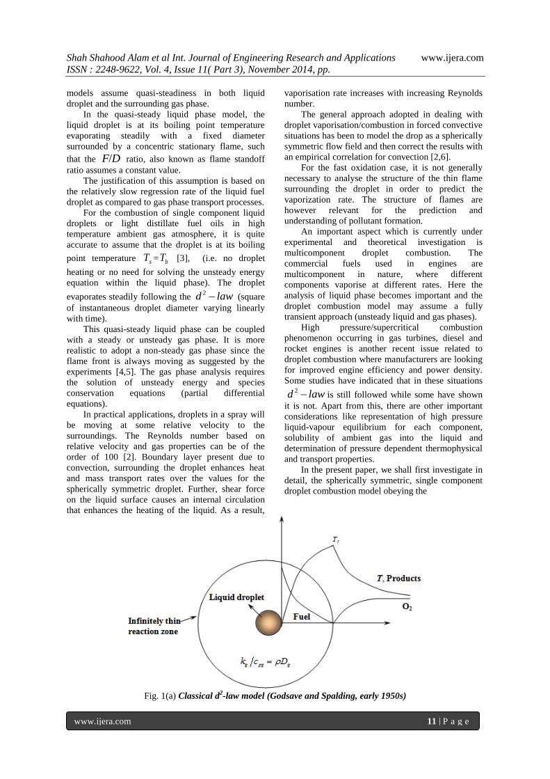
Fig. 1(a) Classical d

2-law model (Godsave and Spalding, early 1950s)

2d law




Fig. 1(b) Relaxation of d

2-law assumption (Law, 1976 and 1980)

, coupled with an unsteady gas phase.

This model shall be extended to include convective

effects. After that, a general variation of species

concentration profiles or emission characteristics

which include CO, CO2, H2O and NO around a

burning fuel droplet shall be obtained using the

unsteady gas phase model described above.

The basic essentials of liquid phase analysis

which are fundamental for developing a realistic

multicomponent droplet evaporation/combustion

model will be taken up next. Finally, we shall be

discussing in brief the important equations and

methodology for developing a high pressure droplet

vaporisation model.

We start with a brief literature review of the

above mentioned droplet sub models.

Kumagai and co-workers [5,7,8] were pioneers

in conducting spherically symmetric droplet

combustion experiments in microgravity conditions

through drop towers, capturing the flame movement

and further showed that F / D ratio varies

throughout the droplet burning history.

Waldman [9] and Ulzama and Specht [10] used

analytical procedure whereas Puri and Libby [11]

and King [12] employed numerical techniques in

developing spherically symmetric droplet

combustion models. The results of these authors

were mainly confined to the observations that unlike

quasi-steady case, flame is not stationary and flame

to droplet diameter ratio increases throughout the

droplet burning period.

A study on convection was carried out by Yang

and Wong [13] who investigated the effect of heat

conduction through the support fibre on a droplet

vaporising in a weak convective field. Another

aspect related to convection is the presence of

internal circulation within the droplet. Law, C.K [14]

introduced the „infinite diffusivity‟ or „batch

distillation‟ model which assumed internal

circulation within the droplet. Droplet temperature

and concentrations were assumed spatially uniform

but temporally varying. It was suggested that the

more volatile substance will vaporise from the

droplet surface leaving only the less volatile material

to vaporise slowly.

In the absence of internal circulation, the

infinite diffusivity model was found to be

inappropriate. For such conditions Landis and Mills

[15] carried out numerical analysis to solve the

coupled heat and mass transfer problem for a

vaporising spherically symmetric, miscible

bicomponent droplet. This model in literature is

termed as „diffusion limit‟ model.

Law, C.K [16] generalised the formulation of

Landis and Mills and suggested that regressing

droplet surface problems are only amenable to

numerical solutions. Tong and Sirignano [17]

devised a simplified vortex model which required

less computing time than the more detailed model of

Lara-Urbaneja and Sirignano [18].

In an experimental investigation, Aldred et al.

[19] used the steady state burning of n-heptane

wetted ceramic spheres for measuring the flame

structure and composition profiles for the flame

corresponding to 9.2mm diameter sphere. Their

results indicated that oxidizer from the ambient

atmosphere and fuel vapour from the droplet surface

diffuse towards each other to form the flame where

the products of combustion are formed and the flame

temperature is highest.

Marchese and Dryer [20] considered detailed

chemical kinetic modelling for the time dependent

burning of isolated, spherically symmetric liquid

droplets of methanol and water using a finite element

chemically reacting flow model. It was noted that a

favourable comparison occurred with microgravity

droplet tower experiment if internal liquid circulation

was included which could be caused by droplet

2d law




generation/deployment techniques. However,

significant deviations from the quasi-steady

were observed.

As mentioned before, the recent trend in the

utilisation of synthetic and derived fuels has

generated renewed interest in the vaporisation and

combustion of multicomponent liquid fuel droplets.

The fuel vaporization process is crucial in

determining the bulk combustion characteristics of

multicomponent fuel spray and its influence on

pollution formation.

For analysing multicomponent droplet

vaporisation/combustion model, the liquid droplet

will not be assumed to be at its boiling point

temperature and therefore the problem becomes

involved, since one has to solve the time dependent

energy equation in the liquid phase in addition to the

transient liquid phase species mass diffusion

equation.

Law and Law [21] formulated a 2d law

model for a spherically symmetric, multicomponent

droplet vaporisation and combustion. It was noted

that the mass flux fraction or the fractional

vaporisation rate m was propotional to the initial

liquid phase mass fraction of that species prior to

vaporisation. The simplified vortex model of Tong

and Sirignano [17] was another valuable contribution

in the analysis of multicomponent droplet

evaporation.

Apart from that, the modelling results of Shaw

[22] suggested that is followed after the

decay of initial transients for the case of spherical

combustion of miscible bicomponent droplets. A

comprehensive experimental investigation was

conducted by Sorbo et al. [23] to quantify the

combustion characteristics of pure CHCS (chlorinated

hydrocarbons) as well as their mixtures with regular

hydrocarbon fuels for enhancing the incinerability of

CHCS.

Some important contributions to high pressure

droplet evaporation and combustion are provided by

the following researchers.

Chin and Lefebvre [3] investigated the effects of

ambient pressure and temperature on steady state

combustion of commercial multicomponent fuels

like aviation gasoline, JP5 and diesel oil (DF2). Their

results suggested that evaporation constant values

were enhanced as ambient pressure and temperature

were increased.

Kadota and Hiroyasu [24] conducted an

experimental study of single suspended alkanes and

light oil droplets under natural convection in

supercritical gaseous environment at room

temperatures. It was noted that combustion lifetime

decreased steeply with an increase in reduced

pressure till the critical point whereas burning

constant showed a continuously increasing trend with

reduced pressure in both sub and supercritical

regimes.

Deplanque and Sirignano [25] developed an

elaborate numerical model to investigate spherically

symmetric, transient vaporisation of a liquid oxygen

(LOX) droplet in supercritical gaseous hydrogen.

They advocated the use of Redlich-Kwong equation

of state (EOS) and suggested it can be assumed that

dissolved hydrogen remains confined in a thin layer

at the droplet surface. Further it was observed that

vaporisation process followed the .

Zhu and Aggarwal [26] carried out numerical

investigation of supercritical vaporisation

phenomena for n-heptane-N2 system by considering

transient, spherically symmetric conservation

equations for both gas and liquid phases, pressure

dependent thermophysical properties and detailed

treatment of liquid-vapour phase equilibrium

employing different equations of state.

II. Problem Formulation 2.1 Development of spherically symmetric droplet

combustion model for the gas phase

As mentioned before, droplet combustion

experiments have shown that liquid droplet burning

is a transient phenomenon. This is verified by the

fact that the flame diameter first increases and then

decreases and flame to droplet diameter ratio

increases throughout the droplet burning unlike the

simplified analyses where this ratio assumes a large

constant value. Keeping this in mind, an unsteady,

spherically symmetric, single component, diffusion

controlled gas phase droplet combustion model is

developed by solving the transient diffusive

equations of species and energy.

Important assumptions invoked in the developmentof

spherically symmetric gas phase droplet combustion

model of the present study

Spherical liquid fuel droplet is made up of single

chemical species and is assumed to be at its boiling

point temperature surrounded by a spherically

symmetric flame, in a quiescent, infinite oxidising

medium with phase equilibrium at the liquid-vapour

interface expressed by the Clausius-Clapeyron

equation.

Droplet processes are diffusion controlled

(ordinary diffusion is considered, thermal and

pressure diffusion effects are neglected). Fuel and

oxidiser react instantaneously in stoichiometric

proportions at the flame. Chemical kinetics is

infinitely fast resulting in flame being represented as

an infinitesimally thin sheet.

Ambient pressure is subcritical and uniform.

Conduction is the only mode of heat transport,

radiation heat transfer is neglected. Soret and Dufour

effects are absent.

2d law

2d law

2d law




Thermo physical and transport properties are

evaluated as a function of pressure, temperature and

composition. Ideal gas behaviour is assumed.

Enthalpy „ h ‟ is a function of temperature only. The

product of density and diffusivity is taken as

constant. Gas phase Lewis number gLe is assumed

as unity.

The overall mass conservation and species

conservation equations are given respectively as:

2

2

10rr v

t r r

(1)

2

2

10r

Y Yr v Y D

t r rr

(2)

Where;

t is the instantaneous time

r is the radial distance from the droplet center

is the density

rv is the radial velocity of the fuel vapour

D is the mass diffusivity

Y is the mass fraction of the species

equations (1) and (2) are combined to give species

concentration or species diffusion equation for the

gas phase as follows

2

2

2 g

g r

DY Y Y YD v

t r r r r

(3)

gD is the gas phase mass diffusivity

The relation for energy conservation can be written

in the following form

2

2

1. 0r p

h Tr v h D C

t r r r

(4)

The energy or heat diffusion equation for the gas

phase, equation (5) can be derived with the help of

overall mass conservation equation (1) and equation

(4), as: 2

2

2 g

g r

T T T Tv

t r r r r

(5)

T is the temperature, g is gas phase thermal

diffusivity. Neglecting radial velocity of fuel vapour

rv for the present model, equations (3) and (5)

reduce to a set of linear, second order partial

differential equations (eqns 6 and 7). 2

2

2 g

g

DY Y YD

t r r r

(6)

2

2

2 g

g

T T T

t r r r

(7)

These equations can be accurately solved with

finite difference technique using appropriate

boundary conditions and provide the solution in

terms of species concentration profiles (fuel vapour

and oxidiser) and temperature profile for the inflame

and post flame zones respectively.

The boundary and initial conditions based on

this combustion model are as follows

, , ; , 0, 0f f o f F fat r r T T Y Y

, ; , 0.232,oat r r T T Y

, 0; , , 1.0lo b F Sat t r r T T Y

1/ 2

where 1 / for 0 ,l lo d dr r t t t t

is the moving boundary condition coming out from

the . Here, fT and T are temperatures

at the flame and ambient atmosphere respectively.

,F SY and ,F fY are fuel mass fractions respectively

at the droplet surface and flame. ,oY and ,o fY are

oxidiser concentrations in the ambience and at the

flame respectively, t is the instantaneous time, dt is

the combustion lifetime of the droplet, lor is the

original or initial droplet radius and lr is the

instantaneous droplet radius at time “ t ”.

The location where the maximum temperature

fT T or the corresponding concentrations

, 0F fY and , 0o fY occur, was taken as the

flame radius fr . Instantaneous time “ t ” was

obtained from the computer results whereas the

combustion lifetime “ dt ” was determined from the

relationship coming out from the 2d law . Other

parameters like instantaneous flame to droplet

diameter ratio ( / )F D , flame standoff distance

( ) / 2F D , dimensionless flame diameter

0( / )F D etc, were then calculated as a function of

time. Products species concentrations (CO, NO, CO2

and H2O) were estimated using Olikara and Borman

code [1] with gas phase code of the present study.

Solution technique

Equations (6) and (7) are a set of linear, second

order, parabolic partial differential equations with

variable coefficients. They become quite similar

when thermal and mass diffusivities are made equal

for unity Lewis number. They can be solved by any

one of the following methods such as weighted

residual methods, method of descritisation in one

variable, variables separable method or by finite

2d law




difference technique. In weighted residual methods,

the solution is approximate and continuous, but these

methods are not convenient in present case since one

of the boundary condition is time dependent. The

method of descritisation in one variable is not

suitable since it leads to solving a large system of

ordinary differential equations at each step and

therefore time consuming. Variables separable

method provides exact and continuous solution but

cannot handle complicated boundary conditions.

Keeping in view the limitations offered by other

methods, “finite difference technique” is chosen

(which can deal efficiently with moving boundary

conditions, as is the case in present study) and

successfully utilised in solving equations (6) and (7).

The approach is simple, fairly accurate and

numerically efficient [27]. Here the mesh size in

radial direction is chosen as h and in time direction

as k . Using finite difference approximations,

equations (6) and (7) can be descritised employing

three point central difference expressions for second

and first space derivatives, and the time derivative is

approximated by a forward difference approximation

resulting in a two level, explicit scheme (eqn 8),

which is implemented on a computer.

1

1 1 1 1 11 1 2 1n n n n

m m m m m mT p T T p T

(8)

Here, 2

1( ) / , /m mmesh ratio k h p h r ,

m lor r mh , 0,1, 2.... . = , ol NNh r r m

The solution scheme is stable as long as the

stability condition 1 1/ 2 is satisfied. Equations

(6) and (7) can also be descritised in Crank-

Nicholson fashion, which results in a six point, two

level implicit scheme. From a knowledge of solution

at the thn time step, we can calculate the solution at

the 1th

n time step by solving a system of

1N tridiagonal equations. Although the resulting

scheme is more accurate, the cost of computation is

fairly high.

Stability condition

The two level explicit scheme given by equation

(8) with an order of accuracy 2(0 ( ))k h is

stable for and is reasonably accurate as

long as stability criterion is obeyed as discussed

below.

Applying Von-Neuman method [27], we write the

error in the form 1 = i mhn n

A em

…… (9)

A is an arbitrary constant, is the amplification

factor and an arbitrary angle. Substituting nm in

place of n

mU in the equation

1

1 1 1 1 11 1 2 1n n n n

m m m m m mU p U U p U

we obtain

1

1 1 1 1 11 1 2 1n n n n

m m m m m mp p

(10)

The solution of the above equation determines the

growth of error in the computed values of .

Substituting from (9) into (10), we obtain after

simplification:

1 1 1 = 2 cos sin (1 2 )h pi h . For

stability, ׀ is less than 1, so that the error remains ׀

bounded and does not tends to infinity. This

condition is only satisfied if .

2.2 Estimation of flame temperature

In the present work, thermodynamic and

transport properties were evaluated on the basis of

flame temperature and ambient temperature for the

outer or the post flame zone and boiling point

temperature and flame temperature for the inner or

inflame zone. Accuracy of the evaluated properties

depend upon the correct estimation of flame

temperature and play a vital role in predicting

combustion parameters and their comparison with

the experimental results. A computer code was

developed in the present work for determining the

adiabatic flame temperature using first law of

thermodynamics with no dissociation effects. A more

accurate method like Gülder [28] (described below)

which incorporates dissociation, multicomponent

fuels and high temperature and pressure effects was

also used for getting flame temperature. An

expression of the following form has been adopted to

predict the flame temperature, which is applicable for

the given ranges:

[0.3 1.6; 0.1 7.5 ;MPa P MPa

275 950 ; 0.8 / 2.5]K Tu K H C

2

.exp . x y z

adiabaticT A

(11)

where,

2

1 1 1

2

2 2 2

2

3 3 3

x a b c

y a b c

z a b c

is dimensionless pressure = / oP P ( oP = 0.1013

MPa )

1 1/ 2

n

mU

1 1/ 2




is dimensionless initial mixture temperature

/u aT T

aT = 300 K

is /H C atomic ratio

= for 1 ( is the fuel-air equivalence ratio

defined as

( / ) /( / )actual stoichiometricF A F A ) and

= 0.7, for >1

Now,

/

/

pf l pa a

u

pf pa

C T A F C T LT

C A F C

(12)

pfC is the specific heat of fuel vapour

paC is the specific heat of air obtained from

standard air tables

lT is the liquid fuel temperature

= (0.363 + 0.000467. bT )(5 - 0.001 fo )

(kJ/kgK)

fo is density of fuel at 288.6 K

bT is boiling point Temperature ( K )

2.40630.2527

0.9479 100mb fT

mbT is the fuel mid boiling point ( K )

f is the relative liquid density of fuel at 20 C

(360 0.39 ) /l fL T /kJ kg (13)

(latent heat of vaporization L can also be evaluated

from Reid et al. [29] )

Once and are known, Table A.1 [28] given in

Appendix A can be consulted for choosing constants

1 1 1 2 2 2 3 3 3, , , , , , , , , , , ,A a b c a b c a b c to be

used in equation (11).

After determining the flame temperature, the

reference or average temperatures for the inflame

and post flame zones respectively can be calculated

using average values given as:

1 ( ) / 2ref b fT T T and 2 ( ) / 2ref fT T T (14)

or by using 1/3 rule [30], given as:

1 (1/ 3) (2 / 3)ref b fT T T and

2 (1/ 3) (2 / 3)ref fT T T (15)

For the present gas phase model, thermodynamic

and transport properties like specific heats, diffusion

coefficients, thermal conductivities, latent heats,

densities, were evaluated as a function of reference

temperature and pressure from different correlations

along with proper mixing rules [29]. Combustion

parameters like heat transfer number TB , burning

constant bk , combustion lifetime of the droplet dt

and mass burning rate fm were then calculated on

the basis of these properties. Effects of forced

convection and droplet heating were also

incorporated.

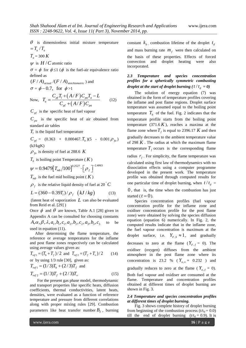
2.3 Temperature and species concentration

profiles for a spherically symmetric combusting

droplet at the start of droplet burning ( / dt t = 0)

The solution of energy equation (7) was

obtained in the form of temperature profiles covering

the inflame and post flame regions. Droplet surface

temperature was assumed equal to the boiling point

temperature of the fuel. Fig. 2 indicates that the

temperature profile starts from the boiling point

temperature (371.6 K ), reaches a maxima at the

flame zone where fT is equal to 2396.17 and then

gradually decreases to the ambient temperature value

of 298 . The radius at which the maximum flame

temperature occurs is the corresponding flame

radius fr . For simplicity, the flame temperature was

calculated using first law of thermodynamics with no

dissociation effects using a computer programme

developed in the present work. The temperature

profile was obtained through computed results for

one particular time of droplet burning, when / dt t =

0 , that is, the time when the combustion has just

started ( 0t ).

Species concentration profiles (fuel vapour

concentration profile for the inflame zone and

oxidiser concentration profile for the post flame

zone) were obtained by solving the species diffusion

equation (equation 6) numerically. In Fig. 2, the

computed results indicate that in the inflame zone,

the fuel vapour concentration is maximum at the

droplet surface, i.e. , 1F SY , and gradually

decreases to zero at the flame ( ,F fY = 0). The

oxidiser (oxygen) diffuses from the ambient

atmosphere in the post flame zone where its

concentration is 23.2 % ( = 0.232 ) and

gradually reduces to zero at the flame ( = 0).

Both fuel vapour and oxidiser are consumed at the

flame. Temperature and concentration profiles

obtained at different times of droplet burning are

shown in Fig. 3.

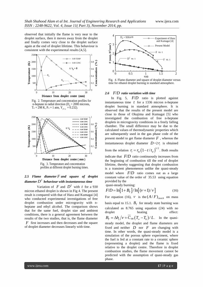
2.4 Temperature and species concentration profiles

at different times of droplet burning.

Fig. 3 shows complete history of droplet burning

from beginning of the combustion process (t/td = 0.0)

till the end of droplet burning (t/td = 0.9). It is

pfC

bT

K

K

fT

,oY

,o fY




observed that initially the flame is very near to the

droplet surface, then it moves away from the droplet

and finally comes very close to the droplet surface

again at the end of droplet lifetime. This behaviour is

consistent with the experimental results [4,5].

2.5 Flame diameter F and square of droplet

diameter2D behaviour with instantaneous time

Variation of and 2D with t for a 930

micron ethanol droplet is shown in Fig 4. The present

result is compared with that of Hara and Kumagai [4]

who conducted experimental investigations of free

droplet combustion under microgravity with n-

heptane and ethyl alcohol. The comparison shows

that for the same fuel, droplet size and ambient

conditions, there is a general agreement between the

results of the two studies, that is, the flame diameter

first increases and then decreases and the square

of droplet diameter decreases linearly with time.

2.6 ratio variation with time

In Fig. 5, ratio is plotted against

instantaneous time for a 1336 micron n-heptane

droplet burning in standard atmosphere. It is

observed that the results of the present model are

close to those of Okajima and Kumagai [5] who

investigated the combustion of free n-heptane

droplets in microgravity conditions in a freely falling

chamber. The small difference may be due to the

calculated values of thermodynamic properties which

are subsequently used in the gas phase code of the

present model to get flame diameter , whereas the

instantaneous droplet diameter D =2 lr is obtained

from the relation 1/ 2

1 /l lo dr r t t . Both results

indicate that ratio continuously increases from

the beginning of combustion till the end of droplet

lifetime, thereby suggesting that droplet combustion

is a transient phenomenon unlike the quasi-steady

model where ratio comes out as a large

constant value of the order of 35.53 using equation

provided by the

quasi-steady burning:

/ ln 1 / ln ( 1) /TF D B (16)

For equation (16), is the ( / )stoichA F on mass

basis equal to 15.1. TB for steady state burning was

calculated as 8.765 using equation (24) with no

droplet heating effect:

/pgT c bB h C T T L . In the quasi-

steady model, the droplet and flame diameters are

fixed and neither nor are changing with

time. In other words, the quasi-steady model is a

simulation of the porous sphere experiment, where

the fuel is fed at a constant rate to a ceramic sphere

(representing a droplet) and the flame is fixed

relative to the droplet centre. Therefore in droplet

combustion studies, the flame movement cannot be

predicted with the assumption of quasi-steady gas

phase.

0 10 20 300

500

1000

1500

2000

2500

0

0.2

0.4

0.6

0.8

1

0.00 TEMP

0.00 CONC

t / td

= 0

Fig. 2. Temperature and concentration profiles forn-heptane in radial direction (D

0= 2000 microns,

T = 298 K, P = 1 atm, Yo, = 0.232).

Co

ncen

trati

on

(%)

Tem

pera

ture

(K)

Distance from droplet centre (mm)

YF

YO

0 10 20 300

500

1000

1500

2000

2500

0

0.2

0.4

0.6

0.8

10.00 TEMP

0.00 CONC

0.30 TEMP

0.30 CONC

0.60 TEMP

0.60 CONC

0.90 TEMP

0.90 CONC

Tem

pera

ture

(K)

Distance from droplet centre ( mm )

Co

ncen

trati

on

(%)

Fig. 3. Temperature and concentrationprofiles at different droplet burning times.

t / td

F

F

0 0.5 1 1.5 20

1

2

3

4

F(m

m),

D2(m

m2)

t (s)

Experiment of Haraand Kumagai [4]

Present Model

F vs t

F vs tD2

vs t

D0

= 930m

Fig. 4. Flame diameter and square of droplet diameter versustime for ethanol droplet burning in standard atmosphere.

/F D

/F Dt

F

/F D

/F D

D F




2.7 Flame diameter F against droplet diameter D

Considering Fig. 6, for the same fuel (n-heptane)

and burning conditions, with 0D = 2000 microns, the

result of the present model shows that flame diameter

increases from an initial value of 1.2cm to a

maximum of 1.5cm, then flame diameter decreases

gradually to a value of 0.48cm. The corresponding

value of droplet diameter D is maximum at the onset

of combustion being equal to the original droplet

diameter 0D (0.2cm), after that it decreases to a

minimum value of about 0.04cm. This variation is in

agreement with the experimental results where flame

diameter first increases and then decreases while

droplet diameter decreases continuously from

beginning to the end of droplet burning period.

2.8 Extension of spherically symmetric gas phase

droplet combustion model to convective

environment

Typical conditions of hydrocarbon fuel droplets

in combustion chambers may have high temperatures

of 1000 K or more, relative velocity between the

droplet surface and ambient gas 10 /m s and

Reynolds number based on relative velocity and gas

properties can be of the order of 100 .

Droplet combustion in convective environment

can be studied in a simpler way by considering a

spherical droplet vaporising with a radial flow field

in the gas phase and then correcting the result with

an empirical correlation for forced convection which

is a function of dimensionless parameters such as

Reynolds number, Prandtl number [6].

For analysing convective droplet combustion,

the following procedure was adopted. The adiabatic

flame temperature fT was first obtained by

considering stoichiometric reaction between air and

fuel (n-octane) using first law of thermodynamics

with no effects of dissociation. The gas phase

mixture properties were then calculated at the

average temperature of fT and T and finally

corrected by applying proper mixing rules.

for n-octane was calculated as 2395 .K

for n-octane fuel vapour as a function of temperature

was determined by Lucas method, air as a function

of temperature was taken from [31]. Then absolute

viscosity of the mixture ( ) or g air fuel vapour

as

a function of temperature was determined from

mixing rules using Wilke method [29], as5 2 5.1483 10 /Ns m

. Other mixture

properties as a function of temperature were

calculated likewise (using appropriate correlations).

Gas phase Reynolds number based on droplet

diameter is given as:

0 /gRe D U (17)

0D is the original droplet diameter, U is the

relative velocity between the droplet surface and the

ambient gas taken as 10 /m s ,

is the density of

the mixture = 0.399 3/kg m . For a chosen droplet

diameter of 1300 m (1.3mm), we

get 100gRe . Then,

-5 =2766 5.1483 10 0.0768 1.854.pgg gPr C

(18)

Here mixture specific heat pgC is in /J kgK and

mixture thermal conductivity g is in /W mK .

Following cases were considered :

(a) Droplet heating with no convection

Then using equation for transfer number:

pgc b

T

pl b

h C T TB

L C T T

(19)

ch is the heat of combustion of fuel

44425 /kJ kg

0 0.5 1 1.5 20

10

20

30

40

50

F/

D

t ( s )

Present Model

Experiment of Okajima and Kumagai [5]

Quasi-steady Model

Fig. 5. Flame to droplet diameter ratio versus timefor a 1336 micron n-heptane droplet burning instandard atmosphere.

F

0 0.05 0.1 0.15 0.20

0.4

0.8

1.2

1.6

F(

cm

)

D ( cm )

Fig. 6. Variation of flame diameter with droplet diameter.

Present Model

fT




is the on mass basis = 15.05

plC as a function of temperature was calculated as

2.15 /kJ kgK

L is the latent heat of vaporisation of fuel

301.92 /kJ kg

bT is the boiling point of fuel =399 K ,

298T K

hence, heat transfer number 5.148TB

using equation (19) for droplet heating, with

5.148TB ,

2

0

8 / ln 1+

ld

g pg T

Dt

C B

(20)

(here, l is density of liquid 3703 /kg m ),

0D is original droplet diameter. Hence, we have

2.945 dt s .

Equation (21) gives the variation of instantaneous

droplet radius lr with instantaneous time " "t ;

0

ln 1l d

lo

r t

g

l l Tpgr tl

r dr B dtC

(21)

Finally, the mass burning rate as a function of time

can be calculated using equation (22),

/ 2f l l bm r k (22)

(b) Droplet heating with convection

Here, dt is modified using equation (20), as

2

0

0.5 0.330.629 s

8 ln 1 1 0.3

ld

g pg T g g

Dt

C B Re Pr

(23)

(with

5.148, 100 and 1.854)T g gB Re Pr

The variation of droplet radius with time can be

determined from equation (21) and mass burning rate

from equation (22).

(c) No droplet heating and no convection (steady

state combustion)

TB at steady state condition is given as:

/ss

pgT c bB h C T T L (24)

Then, 8.851SSTB and using equation (20),

2.33 sSSdt .

Variation of droplet radius with time can be

determined directly from

1/ 2

1 /l lo dr r t t (25)

and as before, mass burning rate from equation (22).

The results are shown in Figs. 7-12. Figs. 7 to 9

show the variation of square of instantaneous droplet

diameter with instantaneous time t , for a n-

octane droplet of 1.3 mm diameter. For the case

when there is steady state burning, (Fig. 7) that is no

droplet heating and no effects of convection, it is

observed that there is a linear variation of 2D with

and the droplet is consumed in approximately

2.4s. Whereas, in Fig. 8, due to droplet heating,

droplet lifetime is increased to about 3 seconds for

the same fuel and burning conditions, however

versus variation is still linear ( is

followed). Fig. 9 shows that when both droplet

heating and convection are considered, droplet is

consumed in a very short time of about 0.63s. If there

had been no droplet heating in presence of

convection, then the lifetime would have been even

lesser.

Figs. 10-12 depict for the same conditions of

fuel, droplet size and ambient conditions the

variation of droplet mass burning rate with

instantaneous time t . From Fig. 10, where there is

no droplet heating and no convection, mass burning

rate is about 0.5 /mg s initially. In Fig. 11, when

droplet heating is considered, the initial mass burning

rate is less than the previous case. This is because as

the droplet heats up to its boiling point, the quantity

of fuel vapour evaporating from the droplet surface is

small and hence mass burning rate is reduced.

Fig. 12 shows the variation of with when

convection is considered with droplet heating. It is

observed that there is an abrupt change in the values

of mass burning rate and droplet lifetime. Due to the

presence of convection the initial mass burning rate

jumps to a value of about 1.92 mg/s and droplet is

consumed in a very short time. Further, if droplet

heating had been ignored in this case, then the initial

mass burning rate would have increased further.

( / )stoichA F

2d law

2D

t

2D

t 2d law

fm

fm t

t (s)

D2

(mm

2)

0 1 2 30

1

2

3D

0= 1.3 mm

Fig. 7. Square of droplet diameter variation with time forn-octane neglecting droplet heating and convection(P = 1 atm, T = 298 K, Y

o, = 0.232).




III. Determination of emission data for a

spherically symmetric burning

droplet Most experiments related to droplet burning

have been concerned primarily with combustion

aspects such as measurement of droplet and flame

temperatures, flame movement, droplet lifetimes,

burning rates etc. As a result less experimental data

related to emission characteristics is available in

literature. Such information is needed to examine the

formation and destruction of pollutants such as soot,

unburned hydrocarbons, NOX, CO and CO2 and

subsequently to establish design criteria for efficient

and stable combustors.

For the determination of species concentration

profiles around the burning spherical droplet, the

following procedure was adopted.

Adiabatic flame temperature determined earlier,

using first law of thermodynamics together with

other input data was used to solve numerically, the

gas phase energy equation (7) with the help of a

computer programme. The solution obtained was in

the form of temperature profile at each time step

starting from the droplet surface, reaching the

maxima at the flame and then reducing to the

ambient temperature value. The radius at which the

maximum temperature occured was taken as the

flame radius.

Temperature values in the vicinity of the flame

were then chosen from the computed results, which

were designated as number of steps ( )NOS . The

solution of species diffusion equation (6) in the gas

phase, gave the species profile (fuel and oxidiser). It

was observed that the fuel vapour concentration was

maximum at the droplet surface and decreased

gradually to the minimum value at the flame front,

whereas, oxygen diffusing from the ambient

atmosphere became minimum at the flame. Now for

the same time step, which was used in the solution of

energy equation, values or NOS of fuel mass

fraction FY corresponding to the temperature values

t (s)

D2

(m

m2

)

0 1 2 30

1

2

3

Fig. 8. Droplet heating with no convection.

0 0.2 0.4 0.60

1

2

3

D2

(m

m2

)

t ( s )

Fig. 9. Droplet heating with convection.

t (s)

mf

(mg

/s)

0 0.5 1 1.5 2 2.5 30

0.25

0.5

0.75

1

Fig. 10. Mass burning rate versus time for n-octaneneglecting droplet heating and convection.

0 1 2 30

0.4

0.8

mf(

mg

/s

)

t (s)

Fig. 11. Droplet heating without convection.

0 0.2 0.4 0.60

0.5

1

1.5

2

mf(m

g/s

)

t (s)

Fig. 12. Droplet heating with convection.




were taken from the computed results of the species

diffusion equation.

Then for a particular fuel, FARS (fuel to air

ratio stoichiometric) on mass basis was calculated for

the stoichiometric reaction of fuel and air at

atmospheric conditions of temperature 298T K ,

pressure 1 P atmosphere and ambient oxidiser

concentration , 0.232oY .

Fuel to air ratio actual ( )FARA on mass basis

was then calculated for each step where,

/1F FFARA Y Y , and finally equivalence ratio,

/FARA FARS . The values of flame

temperature, equivalence ratio and ambient pressure

were then used as input data for the Olikara and

Borman Code [1], (modified for single droplet

burning case) to obtain concentrations of important

combustion products species.

Moreover, since most of the practical

combustion systems operate with air as an oxidiser

therefore formation of NO is a significant parameter

which was another reason for our preference for the

Olikara and Borman programme [1].

3.1 Chemical Equilibrium Composition

The Olikara and Borman model [1] considered

combustion reaction between fuel n m l kC H O N and

air at variable fuel-air equivalence ratio ,

temperatureT and pressure P . Following equation

was considered for representing combustion reaction

between fuel and air:

13 2 2

4 23.7274 0.0444n m l k

n m lx C H O N O N Ar

1 2 3 4 2 5 6 7

8 2 9 2 10 2 11 2 12

x H x O x N x H x OH x CO x NO

x O x H O x CO x N x Ar

(26)

Where 1x through 12x are mole fractions of the

product species and , ,n m l and k are the atoms of

carbon, hydrogen, oxygen and nitrogen respectively

in the fuel. The number n and m should be non-

zero while l and k may or may not be zero.

The number 13x , represents the moles of fuel that

will give one mole of products. In addition to carbon

and hydrogen, the fuel may or may not contain

oxygen and nitrogen atoms. In the present study,

fuels considered were free from nitrogen atoms. The

product species considered [1] were

2 2 2 2 2H,O,N,H ,OH,CO,NO,O ,H O,CO , N and

Ar in gas phase. Whereas in the present work, only

CO, NO, CO2 and H2O were considered for the sake

of simplicity.

The equilibrium constants used in the programme

[1] were fitted as a function of temperature in the

range (600 4000 )K K . It was shown that

equivalence ratio,

0.25 0.5

0.5 0.5

AN AM AL

AN AL

(27)

(where , ,AN AM AL are the number of C, H

and O atoms in fuel molecules). The products of

combustion were assumed to be ideal gases

(assumption not valid at extremely high pressures).

The gas phase code developed in the present work

was used with the Olikara and Borman code [1] for

calculating the equilibrium composition of

combustion products representing species

concentration profiles around a burning droplet.

Important steps of this programme and detailed

kinetic mechanism are given in [1].

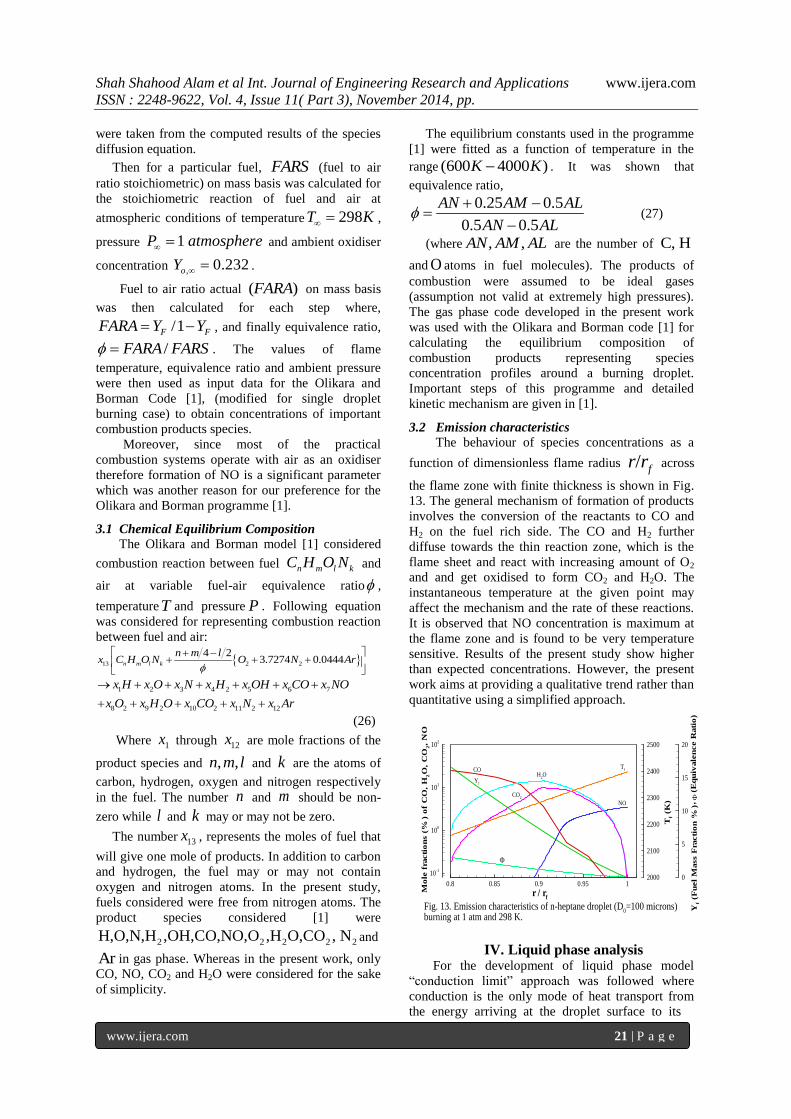
3.2 Emission characteristics

The behaviour of species concentrations as a

function of dimensionless flame radius / fr r across

the flame zone with finite thickness is shown in Fig.

13. The general mechanism of formation of products

involves the conversion of the reactants to CO and

H2 on the fuel rich side. The CO and H2 further

diffuse towards the thin reaction zone, which is the

flame sheet and react with increasing amount of O2

and and get oxidised to form CO2 and H2O. The

instantaneous temperature at the given point may

affect the mechanism and the rate of these reactions.

It is observed that NO concentration is maximum at

the flame zone and is found to be very temperature

sensitive. Results of the present study show higher

than expected concentrations. However, the present

work aims at providing a qualitative trend rather than

quantitative using a simplified approach.

IV. Liquid phase analysis For the development of liquid phase model

“conduction limit” approach was followed where

conduction is the only mode of heat transport from

the energy arriving at the droplet surface to its

0.8 0.85 0.9 0.95 1

10-1

100

101

102

0

5

10

15

20

2000

2100

2200

2300

2400

2500

Mo

lefr

acti

on

s(%

)o

fC

O,

H2O

,C

O2,

NO

Tf(K

)

Yf(F

uel

Mass

Fra

cti

on

%)

(Eq

uiv

ale

nce

Rati

o)

r / rf

H2O

CO2

Tf

Yf

,

Fig. 13. Emission characteristics of n-heptane droplet (D0=100 microns)

burning at 1 atm and 298 K.

CO

NO




interior. Combustion of a n-octane liquid droplet in

ambient conditions of one atmosphere pressure and

298 K was considered. Here, the droplet temperature

is varying both spatially and temporally. The system

is spherically symmetric with no internal liquid

motion. Gas phase is assumed quasi-steady.

Clausius-Clapeyron relation describes the phase

equilibrium at the liquid-vapour interface. The

spherically symmetric, liquid phase heat diffusion

equation or energy equation is given as:

2

2

l l lT Tr

t r rr

=

2

2

2l ll

T T

r r r

(28)

lT and l are liquid phase temperature and thermal

diffusivity respectively.

Initial and boundary conditions being

0,0T r T r (29)

0T ( r ) is the initial temperature distribution

0

0r

T

r

(30)

24

s

l

r

TmH mL

r

(31)

Where sr is the radius at the droplet surface, l is

the liquid thermal conductivity.

The above equation represents the energy

conservation at the interface, L and H are specific

and effective latent heat of vaporisation respectively.

Spherically symmetric, multicomponent liquid phase

mass diffusion equation with no internal circulation

is: 2

, , ,

2

2l m l m l m

l

Y Y YD

t r rr

(32)

,l mY is the concentration or mass fraction of the

m th species in the liquid, and lD is liquid mass

diffusivity which in this case is much smaller than

liquid phase thermal diffusivity l , hence liquid

phase Lewis number, lLe 1.

The boundary condition at the liquid side of the

droplet surface is:

,

,ln 1g gl m

l ms m

l l ls

DYB Y

r D r

(33)

m denotes particular species, lr is the instantaneous

droplet radius at time “ t ”,

fractional mass vaporisation rate, m is species

transfer numberB is the , and gD are

liquid and gas phase mass diffusivities respectively,

l and g are respectively the liquid and gas

phase densities; At the centre of the droplet, symmetry yields

,

0

0l m

r

Y

r

(34)

A uniform initial liquid phase composition for the

droplet was chosen, given as:

, ,0,l m l moY r Y (35)

Equations (28) and (32) are linear, second order

partial differential equations. A convenient method

of solving problems with moving boundary is to

change the moving boundary to a fixed boundary

using coordinate transformation. Hence, equations

(28) and (32) along with the boundary conditions

(equations 28-35) are transformed and solved

numerically using finite difference technique.

The Clausius-Clapeyron relation can be written as

[32]:

1

, {(1 / ( exp([ / ][1/ 1/ ]) 1)}F S g F pg s bY W W P C R T T

(36)

gW is the average molecular weight of all gas phase

species except fuel, at the surface, FW is the

molecular weight of the fuel. R is the specific gas

constant of the fuel, P is equal to one atmosphere,

ands bT T

dimensionless droplet surface and boiling

point temperatures respectively.

Equation (32) with boundary conditions must be

applied concurrently with phase equilibrium

conditions and heat diffusion equation (28) to obtain

the complete solution. For a single component fuel,

phase equilibrium can be expressed by the Clausius-

Clapeyron equation and m (species fractional mass

vaporization rate) is unity. For a multicomponent

fuel, Raoult‟s law provides for the phase equilibrium

and 1.m

4.1 Plot of centre and surface temperatures within

the liquid droplet

The solution of energy equation provides a

plot of droplet surface and centre temperatures as a

function of radial distance at different times of

droplet burning or droplet vaporisation, as the case

may be. The variation of droplet surface temperature

with time then becomes an important input parameter

for the solution of liquid phase mass diffusion

equation.

lD




Fig. 14 shows temperature profiles within a

spherically symmetric n-octane liquid droplet

burning in standard atmosphere. It is observed that as

dimensionless time is increased from an initial value

to about 0.4, droplet surface and center temperatures

become equal to a value corresponding to

approximately 383 K . The droplet heating time is

about 23%. In other words, the heat energy arriving

from the flame is now fully utilized for surface

evaporation and none of the heat is conducted inside

for the purpose of droplet heating, suggesting the

onset of steady state combustion. Fig. 15 depicts the

results of Law and Sirignano [32] for the same

burning conditions. Other important droplet

parameters required are the gas side mole and mass

fractions of each species, transfer number, species

fractional mass vaporisation rate m and

thermodynamic properties of the multicomponent

fuel.

V. Development of droplet

vaporisation model at high pressure Combustion chambers of diesel engines, gas

turbines and liquid rockets operate at supercritical

conditions. To determine evaporation rates of liquid

fuel sprays (made up of discrete droplets) at high

pressures, a prior thermodynamic analysis is a must.

Important assumptions employed in the present high

pressure model are:

Droplet shape remains spherical, viscous

dissipation effects are neglected, ambient gas gets

dissolved in the droplet surface layer only, gas phase

behaves in a quasi-steady manner, radiation heat

transport is neglected and Soret and Dufour effects

are not considered.

At high pressures, vapour-liquid equilibria for

each component can be expressed as: ( ) ( )

1 1

( ) ( )

( ) ( )

v l

v l

v l

f f

T T

P P

(37)

where, the superscripts (v) and (l) stand for vapour

and liquid respectively.

if is the fugacity for component or species “ i ” and

can be integrated through the following relation

, ,

ln [( ) ] lnj

i uu T V u

Vi i

n

f R TPR T dV R T Z

x P n V

(38)

The above equation suggests that can be

determined by the properties of the constituent

components, the concentrations in both phases and

the temperature and pressure of the system. To

compute the integral of the above equation, a real gas

equation of state such as Redlich-Kwong equation of

state was chosen which is given as:

0.5( )

uR T aP

v b v v b T

(39)

Equation (38) is then integrated. After

simplification we get an equation of the form:

1

2

ln ln ln 1 ln ln 1

N

j ij

ji ii i

x ab bA B

f x P Z Z Bb B a b Z

(40)

This equation is valid for both vapour and liquid

phases. The dimensionless parameters A and B are

defined as:

2 2and

u u

aP bPA B

R T R T (41)

Redlich-Kwong equation can be written in the form

of compressibility factor as:

3 2 2 0Z Z A B B Z AB (42)

The mixture compressibility factor “ Z ” can be

determined using Cardan‟s method, where highest

value of Z corresponds to vapour phase and the

smallest value to liquid phase. The parameters a and

b in the cubic equation can be expressed in terms

of composition and pure component

parameters as: 2 2 2

1 1 1

,i j ij i i

i j i

a x x a b x b

(43)

0 0.2 0.4 0.6 0.8 1300

320

340

360

380

Tem

pera

ture

(K

)

Dimensionless Radius

Present Model

Fig. 14. Temporal and Spacial Variationsof Liquid temperatures

0.4

0.17

0.015

0.008

0.08

tnd

= 1.0

0 0.25 0.5 0.75 1300

320

340

360

380

Tem

pera

ture

(K)

Dmensionless Radius

0.5

0.2

0.1

0.04

Model of Law and Sirignano [32]

tnd

= 1.0

0.02

Fig. 15. Modelling results of Law and Sirignano.

if




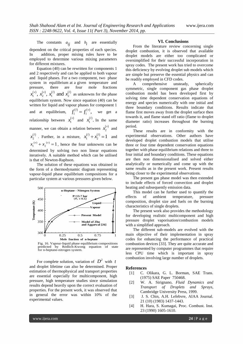
The constants aij and bi are essentially

dependent on the critical properties of each species.

In addition, proper mixing rules have to be

employed to determine various mixing parameters

for different mixtures.

Equation (40) can be rewritten for components 1

and 2 respectively and can be applied to both vapour

and liquid phases. For a two component, two phase

system in equilibrium at a given temperature and

pressure, there are four mole fractions 1 2 1 2, , and

v v l lx x x x as unknowns for the phase

equilibrium system. Now since equation (40) can be

written for liquid and vapour phases for component 1

and at equilibrium,

1 1 ,l v

f f we get a

relationship between 1

vx and

1 .

lx In the same

manner, we can obtain a relation between 2

vx and

2

lx . Further, in a mixture,

1 2 1

l lx x and

( ) ( )

1 2 1v vx x , hence the four unknowns can be

determined by solving two non linear equations

iteratively. A suitable method which can be utilised

is that of Newton-Raphson.

The solution of these equations was obtained in

the form of a thermodynamic diagram representing

vapour-liquid phase equilibrium compositions for a

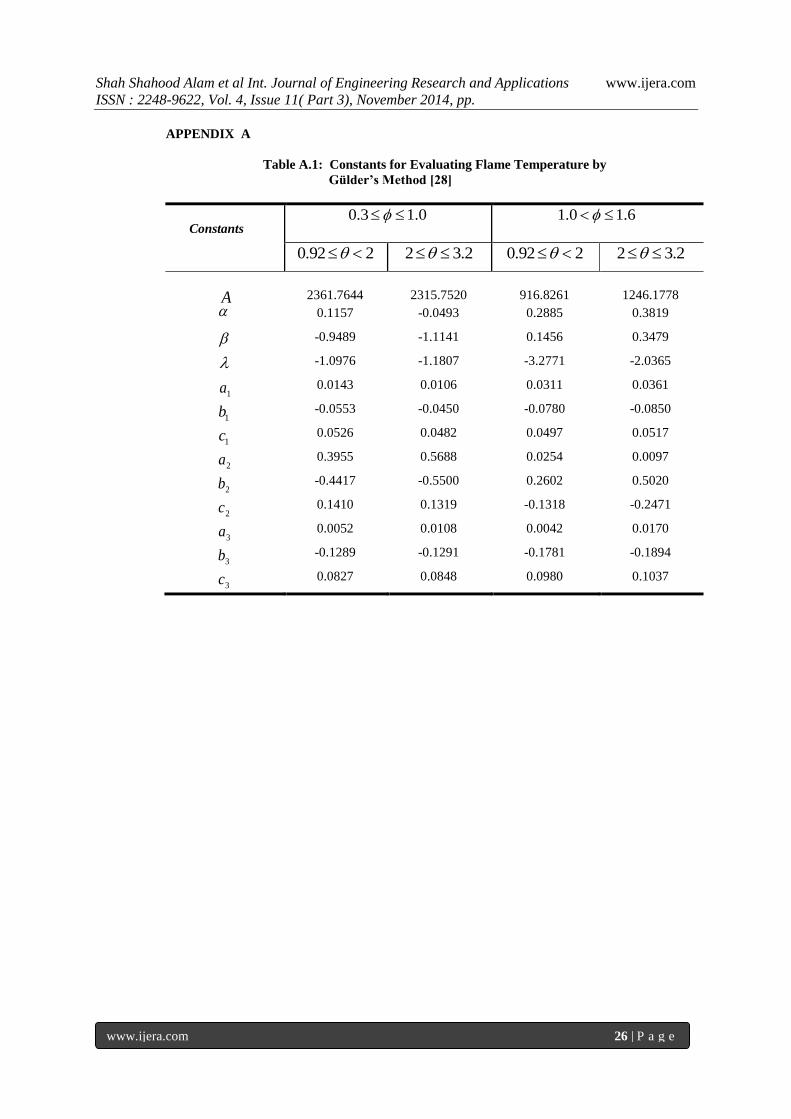
particular system at various pressures given below.

For complete solution, variation of with

and droplet lifetime can also be determined. Proper

estimation of thermophysical and transport properties

are essential especially for multicomponent, high

pressure, high temperature studies since simulation

results depend heavily upon the correct evaluation of

properties. For the present work, it was observed that

in general the error was within 10% of the

experimental values.

VI. Conclusions From the literature review concerning single

droplet combustion, it is observed that available

droplet models are either too complicated or

oversimplified for their successful incorporation in

spray codes. The present work has tried to overcome

this deficiency by evolving droplet sub models which

are simple but preserve the essential physics and can

be readily employed in CFD codes.

A comprehensive unsteady, spherically

symmetric, single component gas phase droplet

combustion model has been developed first by

solving time dependent conservation equations of

energy and species numerically with one initial and

three boundary conditions. Results indicate that

flame first moves away from the droplet surface then

towards it, and flame stand off ratio (flame to droplet

diameter ratio) increases throughout the burning

period.

These results are in conformity with the

experimental observations. Other authors have

developed droplet combustion models that utilise

three or four time dependent conservation equations

together with phase equilibrium relations and three to

four initial and boundary conditions. These equations

are then non dimensionalised and solved either

analytically or numerically and come up with the

same results as in the present work. Present results

being closer to the experimental observations.

The present gas phase model was then extended

to include effects of forced convection and droplet

heating and subsequently emission data.

This model can be further used to quantify the

effects of ambient temperature, pressure

composition, droplet size and fuels on the burning

characteristics of single droplets.

The present work also provides the methodology

for developing realistic multicomponent and high

pressure droplet vaporisation/combustion models

with a simplified approach.

The different sub-models are evolved with the

main objective of their implementation in spray

codes for enhancing the performance of practical

combustion devices [33]. They are quite accurate and

are represented by computer programmes that require

less CPU time which is important in spray

combustion involving large number of droplets.

References [1] C. Olikara, G. L. Borman, SAE Trans.

(1975) SAE Paper 750468.

[2] W. A. Sirignano, Fluid Dynamics and

Transport of Droplets and Sprays,

Cambridge University Press, 1999.

[3] J. S. Chin, A.H. Lefebvre, AIAA Journal.

21 (10) (1983) 1437-1443.

[4] H. Hara, S. Kumagai, Proc. Combust. Inst.

23 (1990) 1605-1610.

0 0.25 0.5 0.75 1300

350

400

450

500

Tem

per

atu

re(K

)

Fig. 16. Vapour-liquid phase equilibrium compositionspredicted by Redlich-Kwong equation of statefor n-heptane-nitrogen system.

n-Heptane - Nitrogen System

P=13.7 bar

Model of Zhuand Aggarwal [26]

Vapour

Liquid

Pr = 0.5( )

Present Model

Mole fraction of n-heptane

2D t




[5] S. Okajima, S. Kumagai, Proc. Combust.

Inst. 15 (1974) 401-407.

[6] G. M. Faeth, Progress in Energy and

Combust. Sci. 3 (1977) 191-224.

[7] S. Kumagai, H. Isoda., Proc. Combust.

Inst. 6 (1957) 726-731.

[8] H. Isoda, S. Kumagai, Proc. Combust. Inst,

7 (1959) 523-531.

[9] C. H. Waldman, Proc. Combust. Inst. 15

(1974) 429-442.

[10] S. Ulzama, E. Specht, Proc. Combust. Inst.

31 (2007) 2301-2308.

[11] I. K. Puri, P. A. Libby, Combust. Sci.

Technol. 76 (1991) 67-80.

[12] M. K. King, Proc. Combust. Inst. 26

(1996) 1227-1234.

[13] J. R Yang, S. C. Wong, Int. J. Heat Mass

Transfer. 45 (2002) 4589-4598.

[14] C. K. Law, Combust. Flame. 26 (1976) 219-

233.

[15] R. B. Landis, A. F. Mills, Fifth Intl. Heat

Transfer Conf. (1974), Paper B7.9, Tokyo,

Japan.

[16] C. K. Law, AIChE Journal. 24 (1978) 626-

632.

[17] A.Y. Tong, W. A. Sirignano, Combust.

Flame. 66 (1986) 221-235.

[18] P. Lara-Urbaneja, W. A. Sirignano, Proc.

Combust. Inst. 18 (1980) 1365-1374.

[19] J. W. Aldred, J. C Patel, A. Williams,

Combust. Flame. 17 (2) (1971) 139-148.

[20] A. J Marchese, F. L. Dryer, Combust.

Flame. 105 (1996) 104-122.

[21] C. K. Law, H. K. Law, AIAA Journal. 20

(4) (1982) 522-527.

[22] B. D. Shaw, Combust. Flame. 81 (1990)

277-288.

[23] N.W. Sorbo, C. K. Law, D. P. Y. Chang and

R. R. Steeper, Proc. Combust. Inst. 22

(1989) 2019.

[24] T. Kadota, H. Hiroyasu, Proc. Combust.

Inst. 18 (1981) 275-282.

[25] J. P. Delplanque, W. A. Sirignano, Int. J.

Heat Mass Transfer. 36 (1993) 303-314.

[26] G. Zhu, S. K. Aggarwal, Int. J. Heat Mass

Transfer. 43 (2000) 1157-1171.

[27] M. K. Jain, Solution of Differential

Equations, Second Edition, Wiley-Eastern

Limited, 1984.

[28] O. L. Gülder, Transac. of the ASME, 108

(1986) 376-380.

[29] R. C. Reid, J. M. Prausnitz, B. E. Poling,

The Properties of Gases and Liquids,

Fourth Edition, McGraw Hill Book

Company, 1989.

[30] G. L. Hubbard, V. E. Denny, A. F. Mills,

Int. J. Heat Mass Transfer, 18 (1975) 1003-

1008.

[31] S. R. Turns, An Introduction to Combustion

Concepts and Applications, McGraw Hill

International Edition, 1996.

[32] C. K. Law, W. A. Sirignano, Combust.

Flame. 28 (1977) 175-186.

[33] G. L. Borman, K. W. Ragland, Combustion

Engineering, McGraw-Hill International

Editions, 1998.




APPENDIX A

Table A.1: Constants for Evaluating Flame Temperature by

Gülder’s Method [28]

Constants

2361.7644 2315.7520 916.8261 1246.1778

0.1157 -0.0493 0.2885 0.3819

-0.9489 -1.1141 0.1456 0.3479

-1.0976 -1.1807 -3.2771 -2.0365

0.0143 0.0106 0.0311 0.0361

-0.0553 -0.0450 -0.0780 -0.0850

0.0526 0.0482 0.0497 0.0517

0.3955 0.5688 0.0254 0.0097

-0.4417 -0.5500 0.2602 0.5020

0.1410 0.1319 -0.1318 -0.2471

0.0052 0.0108 0.0042 0.0170

-0.1289 -0.1291 -0.1781 -0.1894

0.0827 0.0848 0.0980 0.1037

0.3 1.0 1.0 1.6

0.92 2 2 3.2 0.92 2 2 3.2

A

1a

1b

1c

2a

2b

2c

3a

3b

3c

fundamental aspects of droplet combustion modelling

Engineering

droplet mass

droplet combustion models

combustion engineering

droplet heating case

square of droplet diameter

noctane droplet

droplet sub models

nheptane droplet