functional simulation of the integrated onboard system for a commercial launch vehicle

International Refereed Journal of Engineering and Science (IRJES)

ISSN (Online) 2319-183X, (Print) 2319-1821

Volume 3, Issue 11 (November 2014), PP.92-106

www.irjes.com 92 | Page

Functional Simulation of the Integrated Onboard System

For a Commercial Launch Vehicle

Professor Nickolay Zosimovych School of Engineering, Architecture and Health, Tecnologico de Monterrey, Guadalajara,

Av. General Ramon Corona, № 2514, 45201, Jalisco, Mexico. Tel: +52-555-376-5670.

Abstract:- In the article has been chosen and simulated the integrated onboard guidance system of a

commercial launch vehicle with application of GPS technologies. In this study we shall consider a concept of

integrated onboard systems for launch vehicles in the context of the current task, and provide mathematical

models of all its elements for different variants of their structure and composition. Was set the conceptual design

of an integrated navigation system for the space launch vehicle qualified to inject small artificial Earth satellites

into low and medium circular orbits. The conceptual design of the integrated navigation system based on GPS

technology involves determination of its structure, models and algorithms, providing the required accuracy and

reliability in inject payloads with due regard to restrictions on weight and dimensions of the system.

Keywords:- Gimbaled inertial navigation system (GINS), global positioning system (GPS), inertial navigation

system (INS), mathematical model (MM), navigation, pseudorange, pseudovelocity, launch vehicle, self-guided

system (SGS), Kalman filter, control loop, control system (CS), trajectory, boost phase (BPH), distributor,

coordinate, orientation.

I. INTRODUCTION A key tendency in the development of affordable modern navigation systems is displayed by the use of

integrated GPS/INS navigation systems consisting of a gimbaled inertial navigation system (GINS) and a

multichannel GPS receiver [1]. The investigations show [2, 3], that such systems of navigation sensors with

their relatively low cost are able to provide the required accuracy of navigation for a wide class of highly

maneuverable objects, such as airplanes, helicopters, airborne precision-guided weapons, spacecraft, launch

vehicles and recoverable orbital carriers.

Problem setting. The study of applications of GPS navigation technologies for highly dynamic objects ultimately comes

to solving the following problems [4]:

1. Creation of quality standards (optimality criteria) for solving the navigation task depending from the type

of an object, its trajectory characteristics and restrictions on the weights, dimensions, costs, and reliability

of the navigation system.

2. Choosing and justification of the system interconnecting the GPS-receiver and GINS: uncoupled, loosely

coupled, tightly coupled (ultra-tightly coupled).

3. Making mathematical models (MM) of an object's motion, including models of external factors beyond

control influencing object (disturbances). This requires to make two types of object models: the most

detailed and complete one, which will be later included in the model of the environment when simulating

the operation of an integrated system, and a so-called on-board model, which is much simpler and more

compact than the former one, and which will be used in the future to solve the navigation problem being

a part of the on-board software.

4. Making MM for GINS in consideration of use of gyroscopes and accelerometers (i.e. it is required to

make a model for navigation measurements supplied by GINS, taking into account systematic (drift) and

random measurement errors).

5. Making a model of the navigation field of GPS, including system architecture, a method of calculating

ephemeris of navigation satellites in consideration of possible errors, clock drifts on board the navigation

satellites, and taking into account conditions of geometric visibility of a navigation satellite on different

parts of the trajectory of a highly dynamic object.

6. Making a model of a multichannel GPS receiver, including models of code measurements (pseudorange

and pseudovelocity) and, if necessary, phase measurements, including the whole range of chance and

indeterminate factors beyond control, existing when such measurements are conducted (such as multipath

effect).

Functional Simulation of the Integrated Onboard System for a Commercial Launch Vehicle


7. Choosing an algorithm to process measured data in an integrated system in agreement with the speed-of-

response requirement (the possibility to process data in real time) and demanded accuracy in solving a

navigation task.

8. Creating an object-oriented computer complex for the implementation of the above models and

algorithms with the objective to model the process of functioning of the integrated navigation system of a

highly dynamic object.

Let's consider the above objectives, having regard to peculiarities of the subject of inquiry, namely a

commercial launch vehicle, designed to launch payloads into low Earth orbit (LEO) or geostationary orbit

(GSO), in more details.

Within the framework of this study we shall consider a light launch vehicle which has been jointly

developed by the European Space Agency (ESA) and the Italian Space Agency (ASI) since 1998 [5]. It is

qualified to launch satellites ranging from 300 kg to 2000 kg into low circular polar orbits. As a rule, these are

low cost projects conducted by research organizations and universities monitoring the Earth in scientific

missions as well as spy satellites, scientific and amateur satellites. The main characteristics of the launch

vehicle are given in [19]. The launch vehicle Vega [6] is the prototype of the vehicle under development.

The planned payload to be delivered by the launch vehicle to a polar orbit at an altitude of ~700 km

shall be 1500 kg. The launch vehicle is tailored for missions to low Earth and Sun-synchronous orbits. During

the first mission the light class launch vehicle is to launch the main payload, a satellite weighing 400 kg, to an

altitude of 1450 km with an inclination of the orbit 71.500.

The launch vehicle under consideration is the smallest one developed by ESA. We assume that the new

launch vehicle will be able to meet the demands of the market for launching small research satellites and will

enable universities to conduct research in space. The launcher will be primarily used for satellites that monitor

the Earth surface. The injection is conducted according to the most popular and simplest (and the cheapest)

scenario [7, 8], more specifically: the instrument unit and the navigation system ride atop the 3rd stage of the

launch vehicle. Thus, launching until separation of the 4th stage carrying payload is conducted in accordance

with the data provided by the navigation system which estimates 12 components of the launcher state vector,

including position, velocity, orientation angles and angular velocities. Basically, launching may be done upon

implementation of any of the possible algorithms, for example, a terminal one, that provides accuracy of the 3rd

stage launching to the calculated point of separation of the 4th stage or the traditional algorithm which

minimizes the deviation of the center of mass of the launcher from the preselected programmed trajectory [5].

The injection sequence which is being described here supposes conducting the following procedures at

peak altitude reached by the 3rd stage, namely the computation of the required orientation of the 4th stage and

the computation of the required impulse to transfer the payload carried by the 4th stage to an orbit of an artificial

satellite of the Earth from the final point reached by the 3rd stage. Thus, the transfer of the 4th stage from the

end-point of lifting the 3rd stage to an orbit of injecting the payload is performed by the software, i.e. without

the use of navigation data, and thus the accuracy of injection of the payload into the required orbit is determined

by two factors: the accuracy of lifting the 3rd stage in the predetermined terminal point and the accuracy of the

program control in the 4th stage [5].

From the standpoint of the problem concerned, namely the synthesis of the navigational algorithm of

the space launcher in the proposed injection sequence we are interested only in the first factor, i.e. accuracy of

lifting of the 3rd stage to the point of separation 4th stage. This accuracy, other conditions being equal, is

determined by the precision of solving a navigation task in lifting the 3rd stage in consideration of both

components: the center of mass and the velocity of the stage. They predetermine the required impulse for the 4th

stage [9].

Thus, we may determine the main criterion of the accuracy of the navigation task in relation to the

integrated inertial navigation system of the space launch vehicle: we need to ensure maximum accuracy in

determining the position and velocity vectors of the 3rd stage of the launch vehicle in the exo-atmospheric phase

of the mission in the selected for navigation coordinate system. Clearly, this accuracy, in its turn, other things

being equal, depends upon the accuracy of the initial conditions of travel of the 3rd stage, or in other words, the

accuracy of navigation on the previous atmospheric phase of the mission [1].

Consequently, in the case of the proposed injection sequence the simplest and most obvious criterion

for evaluation of the accuracy of the synthesized system should be adopted. It is required to ensure maximum

accuracy in determining the vectors of position and the center -of- mass velocity of the launcher during the

flight of the1st-3rd stages, i.e. in atmospheric and exo-atmospheric phases of the mission. This accuracy can be

characterized by the value of the dispersions posteriori of the corresponding components of the mentioned

vectors [10].



II. MATHERIALS AND METHODS Now let's consider the possible integration schemes for GINS and GPS receiver with respect to this

technical problem [11]. As it has been aforementioned, currently we can think of three possible integration

schemes as follows [12-16]:

uncoupled (separated subsystems);

loosely coupled;

Tightly coupled (ultra-tightly coupled).

Let's consider the peculiarities of these systems.

Uncoupled systems are the simplest option for simultaneous use of INS and GPS receiver [17]. Both

systems operate independently. But, as INS errors constantly accumulate, it is necessary eventually to make

correction of INS according to data provided by the GPS receiver. Creating such architecture requires minimal

changes to the hardware and the software [11].

In loosely coupled systems GINS and GPS also generate separate solutions, but there is a binding unit

in which GPS-based measurements and GINS readouts make assessment of the status vector and make

corrections of data provided by GINS [19].

A loosely coupled complex envisages an independent identification of navigation parameters both by

GINS and Self-Guided System (SGS). Different navigation parameters (coordinates, velocities) are provided by

GINS and SGS. They are then used in the Kalman filter to determine errors occurring in GINS with a purpose of

their subsequent compensation [11, 18].

Such systems usually use two filters: the first one is a part of the satellite receiver, and the second one

is used for co-operative processing of information. The advantage of this scheme is in high functional

reliability of the navigation system. The drawback is in correlation of errors, arriving from SGS to the input of

the second Kalman filter and the need of strict synchronization of measurements provided by INS and SGS [17].

In sources loosely coupled systems are divided into three following types [15]: the standard, "aggressive" and

the so-called MAGR schemes. The difference between "aggressive" scheme and the standard one is that the

former one uses the information on acceleration for extrapolation of navigation sighting executed by SGS

provided by GINS in the period between measurements [11].

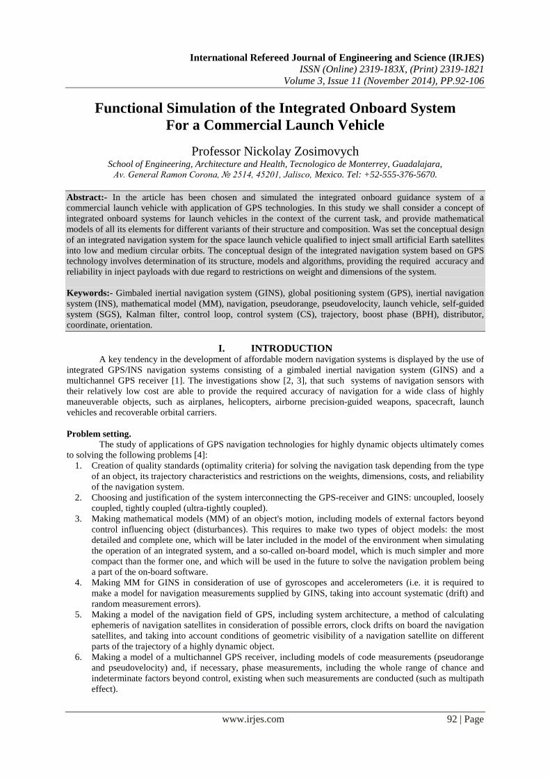
In tightly coupled systems the role of the INS is reduced only to the measurement of the primary

parameters of translational and rotational motions. For this reason, in such systems INS are only inertial

measurement units, and the GPS receiver is without own Kalman filter. In such a structure both INS and SGS

provide a series of measurements for a common computing unit [19].

Tightly coupled systems are characterized by high accuracy compared with aforementioned systems,

and the integrated filter makes it possible to use all available GPS satellites optimal way, but at cost of the

functional redundancy of the system. Tightly coupled systems use the only "evaluator" (as a rule, the Kalman

filter) that uses differences between pseudoranges and/or pseudo velocities, calculated (predicted) by INS and

measured by Self-Guided System. Advantages of such a scheme are the following [6]:

the problem of measurement correlation is absent;

there is no need in synchronization of INS and Self-Guided System as just one clock generator is used;

Search and selection of law quality measurements of pseudorenges.

Fig. 1. Ultra-tightly coupled system [19]



The disadvantages of closely coupled systems are the following [6]:

the need for special equipment for Self-Guided Systems;

use of complex equations for measurements;

Low reliability because INS failure may result if failure of the whole system.

The later drawback can be eliminated by introducing a parallel Kalman filter only for Self-Guided System [11].

Thus, the main differences between a tightly coupled system and a loosely coupled system are as follows:

Use of the INN output information on acceleration in the code and carrier frequency tracking loop. This

allows to narrow the loop bandwidth and improve performance and tuning accuracy;

Use pseudoranges and pseudovelocities (insted of coordinates and velocities) to estimate errors in INS.

A separate embodiment of the tightly coupled systems is the so-called ultra-tightly coupled systems. In such

systems (Fig. 1) estimations are undertaken in the integrated Kalman filter, and the GPS receiver is further

simplified [20]. In this case, the Kalman filter is of order 40 and its implementation requires a computer with a

very high speed [18].

Table 1 Key specification of ultra-tightly coupled MIGITS systems [20]

Specifications C- MIGITS P- MIGITS M- MIGITS

Accuracy:

- coordinates

- velocity

76 m

0,7 m/s

19 m

-

16 m

-

Sizes, mm 146х130х109 146х130х158 -

Number of receiver channels 5L1, C/A 5L1, C/A 10L1, L2, P/Y

Inertial unit GIC-100 IMU-202 DQI (Digital Quartz

IMU)

Operating time between failures,

hours

2700 3600 10000

Weight, kg 2,0 3,2 2,8

Capacity, W 18 20 20

Power supply, V (direct current) 28 28 28

The experience of ultra-tight coupling of inertial and satellite systems is extremely interesting. In

particular, we can meet in sources the so-called MIGITS (Miniature Integrated GPS/INS Tactical Systems)

systems developed by Rockwell International. To date these are the most compact integrated systems [20]. Their

key specifications are presented in Table 1.

III. RESULTS AND DISCUSSION It is known that the algorithm of inertial navigation system is based upon integration of acceleration

values of the launch vehicle sent by integrating accelerometers and reconstruction based upon calculation of the

apparent way of its full position and the velocity in the coordinate system used to solve the navigation task by

taking into account accelerations caused by the gravitational influence of the Earth [11]. Let‟s consider

structures of mathematical methods and algorithms needed to reconstruct all the functions of INS.

The Mathematical Model of INS of the Launch Vehicle Using Gyrostabilized Platform.

In the INS under consideration the main components are the gyrostabilized platform and the block of

integrating accelerometers.

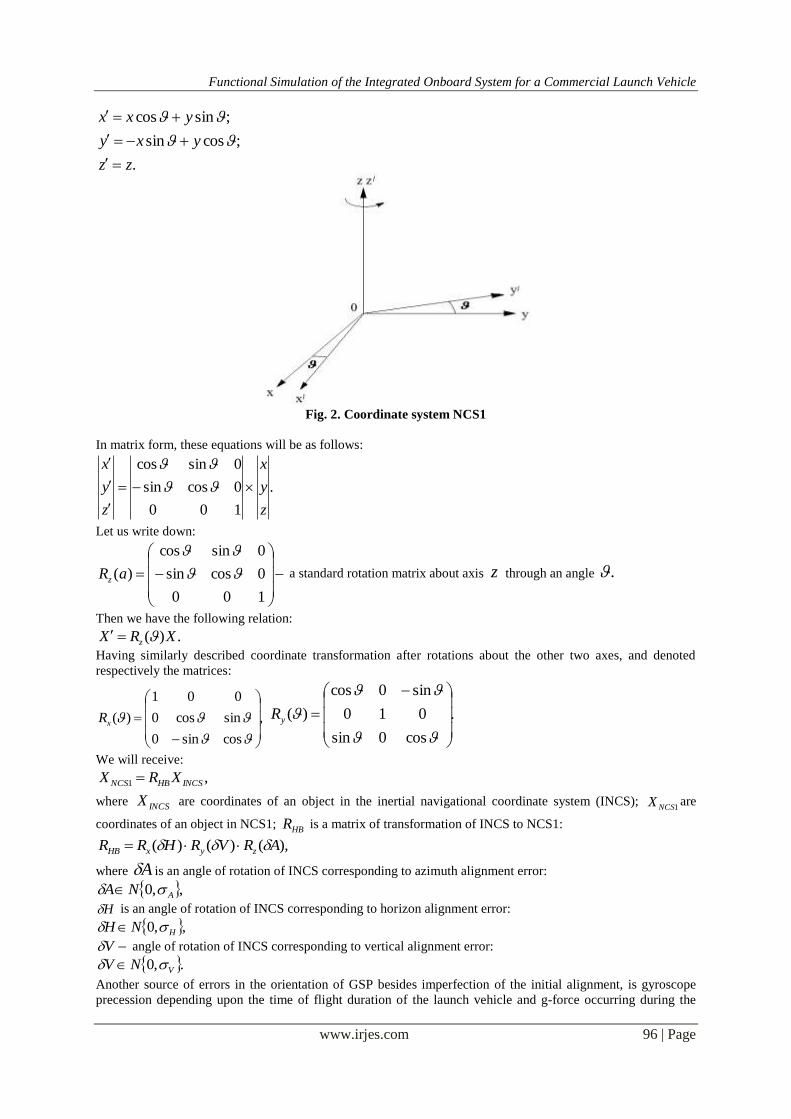
The gyrostabilized platform (GSP) embodies the on-board navigation coordinate system (ONCS).

However, in fact the coordinate system embodied by GSP differs from the ideal NCS due to the following

reasons [21]:

1. Initial alignment of gyrostabilized platform on launch site is imperfect. In other words, orientation of

the axes of the embodied coordinate system (hereinafter referred to as NCS1) differs from the orientation of an

ideal navigation coordinate system (INCS), if latter is adopted as the main coordinate system solving navigation

tasks by initial errors of GSP alignment. This difference is described by a sequence of three turns at angles

corresponding to the initial rotation matrix errors calculated using the following method:

Let us assume that ),,( zyx are the coordinates of a point in the coordinate system .XYZ Then in the

coordinate system ZYX they will rearrange as follows (Fig. 2):



.

;cossin

;sincos

zz

yxy

yxx

Fig. 2. Coordinate system NCS1

In matrix form, these equations will be as follows:

.

100

0cossin

0sincos

z

y

x

z

y

x

Let us write down:

100

0cossin

0sincos

)(

aRz a standard rotation matrix about axis z through an angle .

Then we have the following relation:

.)( XRX z

Having similarly described coordinate transformation after rotations about the other two axes, and denoted

respectively the matrices:

,

cossin0

sincos0

001

)(

xR .

cos0sin

010

sin0cos

)(

yR

We will receive:

,1 INCSHBNCS XRX

where INCSX are coordinates of an object in the inertial navigational coordinate system (INCS); 1NCSX are

coordinates of an object in NCS1; HBR is a matrix of transformation of INCS to NCS1:

),()()( ARVRHRR zyxHB

where A is an angle of rotation of INCS corresponding to azimuth alignment error:

,,0 ANA

H is an angle of rotation of INCS corresponding to horizon alignment error:

,,0 HNH

V angle of rotation of INCS corresponding to vertical alignment error:

.,0 VNV

Another source of errors in the orientation of GSP besides imperfection of the initial alignment, is gyroscope

precession depending upon the time of flight duration of the launch vehicle and g-force occurring during the



flight, and it leads to the so-called drift of GSP. The drift of gyroplatform caused by angular drift can be

described by the following matrix [22, 23]:

),( GSPGSP MED

where ,

0

0

0

12

13

23

GSPM ),,( 321 is a gross error in the orientation of GSP axes in

projection onto INCS axes.

Dynamics of drift shall be described as follows [24, 25]:

,1 tii

where ii ,1 is a gross error corresponding to point in time ;,1 ii tt

t is a total “drift” of GSP axes within time interval .t

In its turn, t may be represented as a sum of “free” GSP drift which is a time function, i.e. independent of

external factors but dependent merely on time, and deviation in the orientation of the axes caused by g-forces

[23, 26]:

,11

Wtg

Mtt CB

where CB is a vector of “free” drift of GSP axes;

,

10

10

01

133

222

111

yZ

HPy

kZ

HPy

kZ

HPy

tg

W

tg

W

tg

W

M

where iy is a vector of the drift speed of axes which is proportional to acceleration;

ik is a vector of the drift

speed of GSP axes due to errors in disbalance of GSP gyroscopes during acceleration acting towards kinematic

moments; iHP is a vector of the drift speed of GSP axes due to lack of rigidity errors.

Increment of apparent velocity is measured using the block of integrating accelerometers. The block of

accelerometers has alignment errors, as is the case with the gyro platform. Simulation of the errors shall be

made according to a scheme similar to the simulation of initial alignment errors for GSP [25, 27], and the

corresponding matrix aR describing transformation from the coordinate system RCS2 materialized through

actual alignment of accelerometers to the onboard navigation coordinate system (ONCS) is the following [28]:

),()()( ZRYRXRR zyxa

where ZYX ,, are angles corresponding to errors in the orientation of the block of accelerometers.

Besides, the gain of each accelerometer is, strictly speaking, a random variable. In addition, measurements

performed by each accelerometer are accompanied by additive measurement error interpreted herein as a

random variable [29].

Against this background, the simulation algorithm for measurement of increment of the apparent velocity read

from accelerometers can be represented as follows [30]:

1. Suppose that the vector of real apparent velocity increment is .INCSW Then, after transformation

INCS into the onboard navigation coordinate system (ONCS), we obtain apparent velocity increment vector in

ONCS:

.INCSHBGSPaONCS WRDRW

2. The values of the components of the apparent velocity increment vector read from accelerometers shall

be calculated according to the following equations

,)(

;)(

;)(

zzONCSACC

yyONCSACC

xxONCSACC

SWWW

SWWW

SWWW

zz

yy

xx

where T

zyx WWWW ),,( is a vector of random measurement errors;



zyx SSS ,, are values of the gain of accelerometers.

Additionally, accelerometers have deadband areas, so increment of the apparent velocity transferred by

accelerometers is compared with a certain threshold value. If the value ACCW is less than the threshold value,

the output value will be 0.

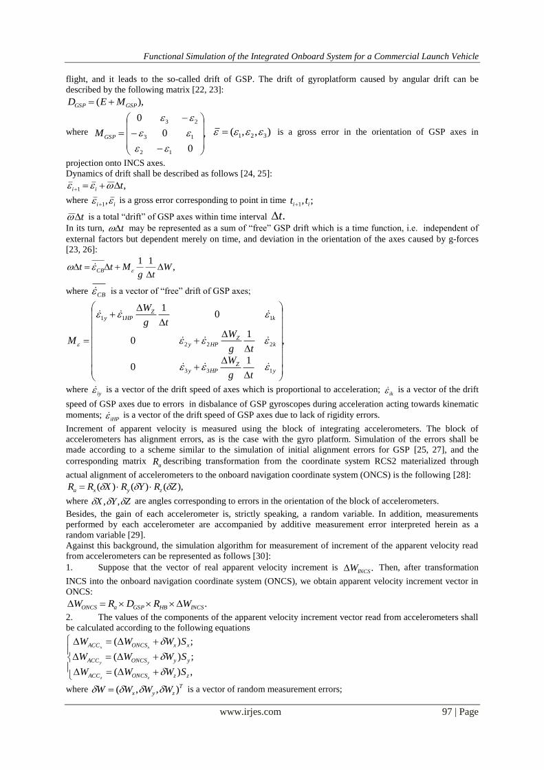
A functional diagram of the model of the onboard measuring system (OMS) is shown in Fig. 3.

Fig. 3. Functional model of OMS

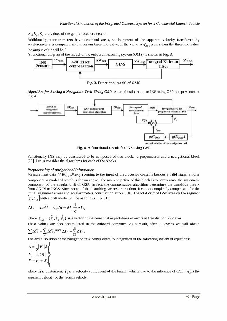
Algorithm for Solving a Navigation Task Using GSP. A functional circuit for INS using GSP is represented in

Fig. 4.

Fig. 4. A functional circuit for INS using GSP

Functionally INS may be considered to be composed of two blocks: a preprocessor and a navigational block

[28]. Let us consider the algorithms for each of the blocks.

Preprocessing of navigational information

Measurement data ),,,( OMSW coming to the input of preprocessor contains besides a valid signal a noise

component, a model of which is shown above. The main objective of this block is to compensate the systematic

component of the angular drift of GSP. In fact, the compensation algorithm determines the transition matrix

from ONCS to INCS. Since some of the disturbing factors are random, it cannot completely compensate for the

initial alignment errors and accelerometers construction errors [18]. The total drift of GSP axes on the segment

1

,ii

tt with a drift model will be as follows [15, 31]:

,1

izCBiW

gMtt

where )ˆ,ˆ,ˆ( 321 CB is a vector of mathematical expectations of errors in free drift of GSP axes.

These values are also accumulated in the onboard computer. As a result, after 10 cycles we will obtain

61

1

,i

and

61

1

.i

WW

The actual solution of the navigation task comes down to integration of the following system of equations:

kg

g

WVX

XgV

F

),(2

1

where is quaternion; gV is a velocity component of the launch vehicle due to the influence of GSP;

kW is the

apparent velocity of the launch vehicle.



The first equation describes the dynamics of the quaternion which directly shows transfer of ONCS from

INCS, where the matrix *E is actually a fundamental matrix of the system of differential equations for the

components of the quaternion:

0

0

0

0

*

zyx

zxy

yxz

xyz

E

The solution of this equation is the vector , which dimensions are 4x1, on which basis the transition matrix to

INCS is built:

)()(2)(2

)(2)()(2

)(2)(2)(

2

2

2

1

2

3

2

010322031

1032

2

3

2

1

2

2

2

03021

20313021

2

3

2

2

2

1

2

0

R

Next, on the basis of the position vector of the launch vehicle calculated in the previous cycle we may calculate

).(Xg It is necessary to recalculate the position vector X of the launch vehicle in EGCS (the equivalent gyro

coordinate system) [6]. This shall be done as follows:

1. The vector X shall be initially transferred to ICS. The transfer is done using standard rotation matrices

with the following arguments:

),90()(90(

,

zxy

T

INCSICS

RRAzRA

XAX

where .56,38,108 000 Az

2. Transfer from ICS to EGCS shall be made. ICS differs from EGCS by orientation of the axes

x and .y So, transfer to EGCS may be made by one turn about the axis :z

,ICSЕGСS ХВX

),(SRВz

where )( 00 ttSS is an angle between the Vernal Equinox direction and the Greenwich meridian [32];

0S is an angle between the Vernal Equinox direction at the beginning of the epoch ;0

t is the angular

velocity of rotation of the Earth; t is the current time.

Then using the position vector in EGCS we shall calculate the new value of the acceleration ),(Xg and then

perform the inverse coordinate transformations:

,ЕGСS

T

ICS gBg

.ICS

T

ICS gAg

Knowing the new value of acceleration ),(Xg we are able to solve the second and the third equations of the

system. As a result, we shall define a new position vector for the launch vehicle. Hereafter the algorithm of INS

will be repeated.

Mathematical Model of INS of the Launch Vehicle with Strapdown Inertial Navigation System (SINS).

When SINS is used, the source of navigation information will be a block of integrating accelerometers

oriented along the body axes of the launch vehicle, and the meter of absolute angular velocity comprising three

high-speed gyros (rate gyros) oriented as well along three mutually perpendicular axes [33].

The models of accelerometers and rate gyros described below have fair number of common features, and will be

used in particular in the modeling of the processes occurring in the model of the environment. Let‟s represent

accelerometer errors occurring in SINS as follows [28]:

;

,

,

54321

54321

54321

zzzyzxzzz

yzyyyxyyy

xzxyxxxxx

nnnn

nnnn

nnnn

(1)

where ),,(1 zyxii are constant displacements of zero of accelerometers;



),,(2 zyxii are accelerometers‟ measurement noise;

543 ,, zyx are accelerometer scale factor errors;

435354 ;;;;; zzyyxx are errors occurring due to nonorthogonality and misalignment of accelerometer

response axes;

zyx nnn ,, are components of the acceleration vector in the associated coordinate system.

Rate gyros‟ errors zyx

,, may be represented as well as the following rather general model [15]:

;

,

,

87654321

87654321

87654321

zzzzzzyzxzzz

yyyyzyyyxyyy

xxxxzxyxxxxx

nnn

nnn

nnn

(2)

where )2,1;,,( jzyxiij are drift invariables of rate gyros and their random measurement noises;

)5,4,3;,,( jzyxiij are specific drift speeds of gyroscopes proportional to g-forces (causes for such

dependence may be different for different types of rate gyros, for example, in mechanical gyroscopes such

dependence can be explained by imbalance of rate gyros);

876 ,, zyx are scale factor errors of rate gyros;

768687 ,,,,, zzyyxx are drifts occurring due to nonorthogonality and misalignment of response axes

of rate gyros;

,, are projections of absolute angular velocity onto INCS axes.

Noise terms of accelerometer errors ),,(2

zyxii

and rate gyros ),,(2

zyxii

appear as stationary

random processes with zero mathematical expectation and the following correlation functions [30, 34-36]:

;

,

2

2

w

n

h

ww

h

nn

eK

eK

where wn , are root-mean-square deviations (RMSD) of the variables 22

,ii

from their mean; wn hh , are

attenuation coefficients of correlation functions for random errors of accelerometers and gyroscopes

respectively.

As knowing, differential equations for generating filters for the mentioned random processes with stationary

input signals such as white noise are as follows [37, 38]:

;2

,2

222

122

iwwiwi

innini

hh

hh

In the above referred models of errors occurring in rate gyros and accelerometers in different parts of the flight

trajectory contribution of the individual components can vary greatly [28]. So when considering the movement

of the launch vehicle at a speed close to constant one along straight trajectories, constant errors occurring in

meters will have major influence [18]. Therefore, in such parts of the trajectory models (1)-(2) may be

significantly simplified, which will facilitate solving of tasks set for the onboard measuring system.

Furthermore, when time correlation coefficients 1

nh and

1

wh are relatively small when compared to the Schuler

period 5064( Sh

T s), processes ),,(, 22 zyxiii approach to "white noise" with certain intensity. Taking

this into consideration, we may present models of gyroscope and accelerometer errors as follows [39]:

;

,

22

11

iiii

iiii

Q

Qn

where ii , are constant errors occurring in meters;

21, ii QQ are intensities of random errors occurring in

meters.

Thus, taking errors of inertial meters into consideration, measurement process of apparent acceleration and

angular velocity taken from the accelerometers and rate gyros can be represented as follows. Values of the

components of the apparent acceleration vector taken from the accelerometers shall be calculated according to

the following equations:



.

,

,

zzSINS

yySINS

xxSINS

nnn

nnn

nnn

z

y

x

Values of the components of angular velocity vector taken from rate gyros shall be calculated according to the

following equations:

,

,

,

zzOMS

yyOMS

xxOMS

z

y

x

where zyxzyx nnn ,,,,, are components of error vectors introduced herein above;

zyxzyx nnn ,,,,, are actual values of measured navigational parameters.

The Algorithm for Solving a Navigation Task when a Strapdown Inertial Navigation System (SINS) is Used.

A functional diagram for SINS operation is presented in Fig. 5.

Fig. 5. A functional diagram for SINS operation

SINS start functioning a few seconds before liftoff and stops after cutoff of the last stage (at the end of the

powered flight phase). As a rule, the navigation task is solved with the help of SINS installed aboard a launcher

with a frequency of 1Hz.

Functionally, the algorithm for solving the navigation task using SINS may be splitted into two blocks:

an integration block for navigation equations;

a block for orientation finding.

As we mentioned earlier, a system of the following motion equations is solved once a second:

,

);(

;

;2

1

BOIF Cnn

XgnV

VX

E

where are Rodrigues-Hamilton parameters fully describing the orientation of the launch vehicle; n is a vector

of apparent acceleration of the launch vehicle; )(Xg is a gravitational vector.

The first three equations of this system are essentially the same as the corresponding equations describing the

algorithm for solving the task by using a gyro-stabilized platform.

The last equation, characteristic only for SINS, describes the process of "reprojection" of the measured

components of acceleration on measuring axes using matrix C, which algorithm is given below.

Algorithm for determining the orientation of LV 1. Calculate item values for matrix C directional cosines between the reference frame attributed to the

launch vehicle and the geographical reference frame:

,

22

22

22

2

2

2

1

2

3

2

010322031

1032

2

3

2

1

2

2

2

03021

20313021

2

3

2

2

2

1

2

0

C



where 3,...,0, ii are elements of the quaternion .

2. Calculate the orientation parameters of the launch vehicle (pitch, roll and yaw):

;1

arcsin2

31

11

C

C

;1

arcsin2

31

33

C

C

(3)

.arcsin 31C

3. Signals received from the accelerometers are translated into INCS to be used in the first navigation

algorithm (the third equation of (3):

,

333231

232221

131211

Z

Y

X

Z

Y

X

OMS

OMS

OMS

INCS

INCS

INCS

n

n

n

CCC

CCC

CCC

n

n

n

where iXOMSn are projections of the apparent acceleration done by accelerometers.

The algorithm is used for the initial orientation of SINS on Earth. The initial orientation is carried out by method

of vector adjustment from measurements of two non-collinear vectors by SINS (accelerometers, gyroscopes) of

the vector of absolute angular velocity of launch vehicle rotation, gravity vector g [33, 40].

4. Algorithm for computing the matrix orientation between the basis connected with vehicle-bound

coordinate system and INCS:

.

22

22

22

2

2

2

1

2

3

2

010322031

1032

2

3

2

1

2

2

2

03021

20313021

2

3

2

2

2

1

2

0

C

5. Algorithm for computing angular orientation parameters of the launch vehicle:

;1

arcsin2

31

11

C

C

;1

arcsin2

31

33

C

C

.arcsin 31C

6. The algorithm for conversion of signals obtained with accelerometers in INCS to be used in the first

navigation algorithm:

,

333231

232221

131211

Z

Y

X

Z

Y

X

OMS

OMS

OMS

INCS

INCS

INCS

n

n

n

CCC

CCC

CCC

n

n

n

where iOMSn are projections of the apparent acceleration measured by accelerometers.

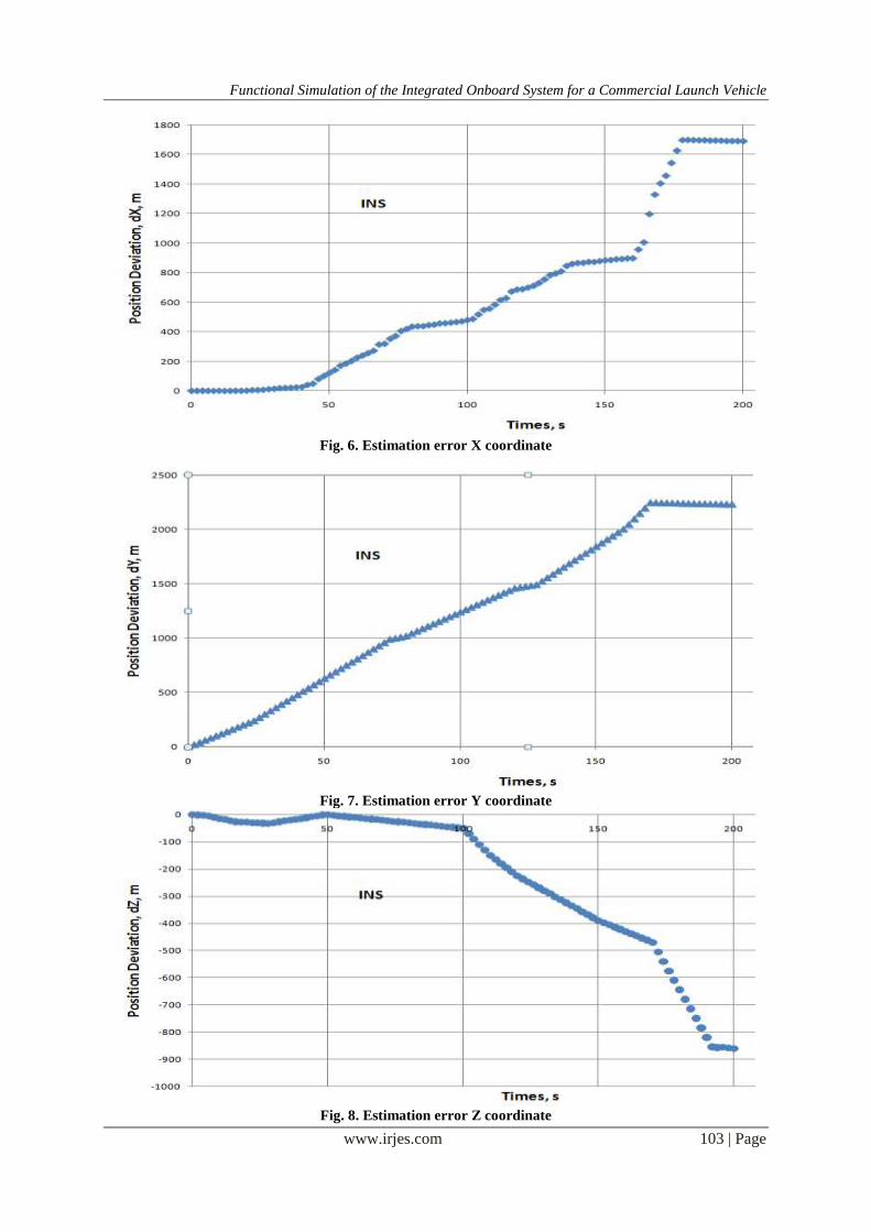
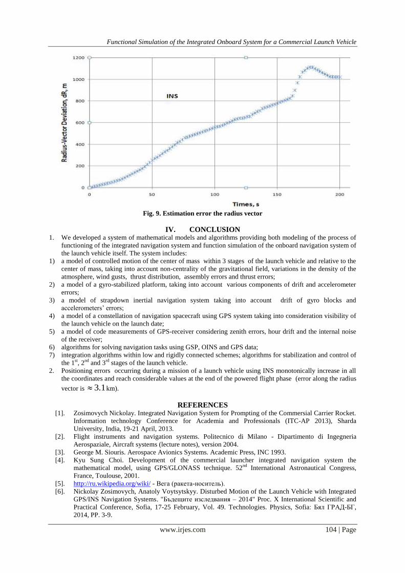
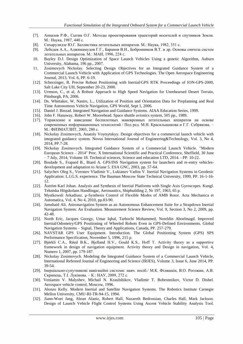
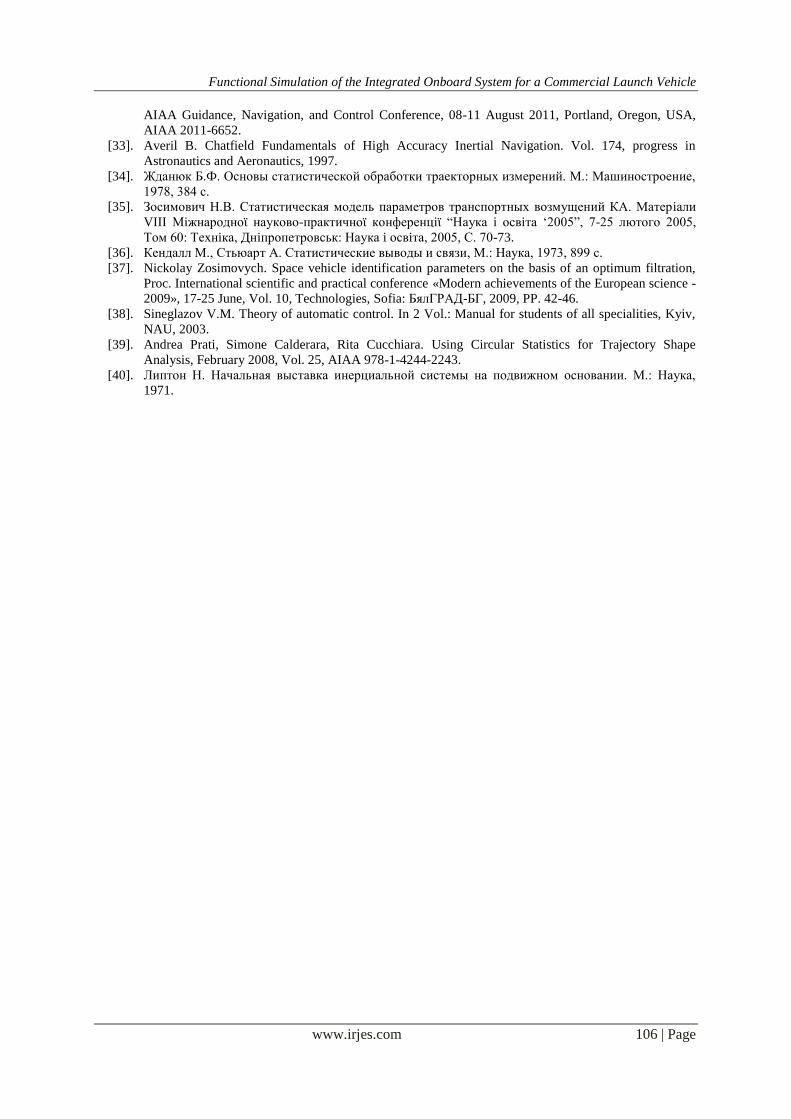
The results of simulation. Based on the conducted simulations have been obtained depending that presented in

Fig.6-9.



Fig. 6. Estimation error X coordinate

Fig. 7. Estimation error Y coordinate

Fig. 8. Estimation error Z coordinate



Fig. 9. Estimation error the radius vector

IV. CONCLUSION 1. We developed a system of mathematical models and algorithms providing both modeling of the process of

functioning of the integrated navigation system and function simulation of the onboard navigation system of

the launch vehicle itself. The system includes:

1) a model of controlled motion of the center of mass within 3 stages of the launch vehicle and relative to the

center of mass, taking into account non-centrality of the gravitational field, variations in the density of the

atmosphere, wind gusts, thrust distribution, assembly errors and thrust errors;

2) a model of a gyro-stabilized platform, taking into account various components of drift and accelerometer

errors;

3) a model of strapdown inertial navigation system taking into account drift of gyro blocks and

accelerometers‟ errors;

4) a model of a constellation of navigation spacecraft using GPS system taking into consideration visibility of

the launch vehicle on the launch date;

5) a model of code measurements of GPS-receiver considering zenith errors, hour drift and the internal noise

of the receiver;

6) algorithms for solving navigation tasks using GSP, OINS and GPS data;

7) integration algorithms within low and rigidly connected schemes; algorithms for stabilization and control of

the 1st, 2

nd and 3

rd stages of the launch vehicle.

2. Positioning errors occurring during a mission of a launch vehicle using INS monotonically increase in all

the coordinates and reach considerable values at the end of the powered flight phase (error along the radius

vector is 1.3 km).

REFERENCES [1]. Zosimovych Nickolay. Integrated Navigation System for Prompting of the Commersial Carrier Rocket.

Information technology Conference for Academia and Professionals (ITC-AP 2013), Sharda

University, India, 19-21 April, 2013.

[2]. Flight instruments and navigation systems. Politecnico di Milano - Dipartimento di Ingegneria

Aerospaziale, Aircraft systems (lecture notes), version 2004.

[3]. George M. Siouris. Aerospace Avionics Systems. Academic Press, INC 1993.

[4]. Kyu Sung Choi. Development of the commercial launcher integrated navigation system the

mathematical model, using GPS/GLONASS technique. 52nd

International Astronautical Congress,

France, Toulouse, 2001.

[5]. http://ru.wikipedia.org/wiki/ - Вега (ракета-носитель).

[6]. Nickolay Zosimovych, Anatoly Voytsytskyy. Disturbed Motion of the Launch Vehicle with Integrated

GPS/INS Navigation Systems. "Бъдещите изследвания – 2014" Proc. X International Scientific and

Practical Conference, Sofia, 17-25 February, Vol. 49. Technologies. Physics, Sofia: Бял ГРАД-БГ,

2014, PP. 3-9.

http://ru.wikipedia.org/wiki/



[7]. Аппазов Р.Ф., Сытин О.Г. Методы проектирования траекторий носителей и спутников Земли.

М.: Наука, 1987, 440 с.

[8]. Сихарулидзе Ю.Г. Баллистика летательных аппаратов. М.: Наука, 1982, 351 с.

[9]. Лебедев А.А., Аджимамудов Г.Г., Баранов В.Н., Бобронников В.Т. и др. Основы синтеза систем

летательных аппаратов. М.: МАИ, 1996, 224 c.

10. Bayley D.J. Design Optimization of Space Launch Vehicles Using a genetic Algorithm, Auburn

University, Alabama, 196 pp., 2007.

11. Zosimovych Nickolay. Selecting Design Objectives for an Integrated Guidance System of a

Commercial Launch Vehicle with Application of GPS Technologies. The Open Aerospace Engineering

Journal, 2013, Vol. 6, PP. 6-19.

[12]. Scherzinger, B. Precise Robust Positioning with Inertial/GPS RTK Proceedings of ION-GPS-2000,

Salt Lake City UH, September 20-23, 2000.

[13]. Urmson, C., et al, A Robust Approach to High Speed Navigation for Unrehearsed Desert Terrain,

Pittsburgh, PA, 2006.

[14]. Ds. Whittaker, W, Nastro, L., Utilization of Position and Orientation Data for Preplanning and Real

Time Autonomous Vehicle Navigation, GPS World, Sept 1, 2006.

[15]. Daniel J. Biezad. Integrated Navigation and Guidance Systems. AIAA Education Series, 1999.

[16]. John F. Hanaway, Robert W. Moorehead. Space shuttle avionics system, 505 pp., 1989.

[17]. Управление и наведение беспилотных маневренных летательных аппаратов на основе

современных информационных технологий / Под ред. М.Н. Красильщикова и Г.Г. Себрякова. –

М.: ФИЗМАТЛИТ, 2003, 280 с.

[18]. Nickolay Zosimovych, Anatoly Voytsytskyy. Design objectives for a commercial launch vehicle with

integrated guidance system. Novus International Journal of Engineering&Technology, Vol. 3, No 4,

2014, PP.7-28.

[19]. Nickolay Zosimovych. Integrated Guidance System of a Commercial Launch Vehicle. "Modern

European Science – 2014" Proc. X International Scientific and Practical Conference, Sheffield, 30 June

– 7 July, 2014, Volume 18. Technical sciences, Science and education LTD, 2014. - PP. 10-22.

[20]. Boulade S., Frapard B., Biard A. GPS/INS Navigation system for launchers and re-entry vehicles-

development and adaptation to Ariane 5. ESA GNC, 2003, pp. 57-64.

[21]. Salychev Oleg S., Voronov Vladimir V., Lukianov Vadim V. Inertial Navigation Systems in Geodesic

Application: L.I.G.S. experience. The Bauman Moscow State Technical University, 1999, PP. 16-1-16-

12.

[22]. Åström Karl Johan. Analysis and Synthesis of Inertial Platforms with Single Axis Gyroscopes. Kungl.

Tekniska Högskolans Handlingar, Aeronautics, Shipbuilding 2, Nr 197, 1963, 65 p.

[23]. Mystkowsli Arkadiusz. µ-Synthesis Control of Flexible Modes of AMB Rotor. Acta Mechanica et

Automatica, Vol. 4, No 4, 2010, pp.83-90.

[24]. Jamshaid Ali. Astronavigation System as an Autonomous Enhancement Suite for a Strapdown Inertial

Navigation System: An Evaluation. Measurement Science Review, Vol. 9, Section 3, No 2, 2009, pp.

42-48.

[25]. North Eric, Jacques Georgy, Umar Iqbal, Tarbochi Mohammed, Noreldin Aboelmagd. Improved

Inertial/Odometry/GPS Positioning of Wheeled Robots Even in GPS-Defined Environments. Global

Navigation Systems – Signal, Theory and Applications, Canada, PP. 257-279.

[26]. NAVSTAR GPS User Equipment. Introduction. The Global Positioning System (GPS) SPS

Performance Specification, November 5, 1996, 215 p.

[27]. Bjǿrkli C.A., Rǿed B.K., Bjelland H.V., Gould K.S., Hoff T. Activity theory as a supportive

framework in design of navigation equipment. Activity theory and Design in navigation, Vol. 4,

Numero 1, 2007, pp. 179-187.

[28]. Nickolay Zosimovych. Modeling the Integrated Guidance System of a Commercial Launch Vehicle,

International Refereed Journal of Engineering and Science (IRJES), Volume 3, Issue 6, June 2014, PP.

39-54.

[29]. Інерціально-супутникові навігаційні системи: навч. посіб./ М.К. Філяшкін, В.О. Рогожин, А.В.

Скрипець, Т.І. Лукінова. – К.: НАУ, 2009, 272 с.

[30]. Veniamin V. Malyshev, Michail N. Krasilshikov, Vladimir T. Bobronnikov, Victor D. Dishel.

Aerospace vehicle control, Moscow, 1996.

[31]. Alonzo Kelly. Modern Inertial and Satellite Navigation Systems. The Robotics Institute Carnegie

Mellon University, CMU-RI-TR-94-15, 1994.

[32]. Jiann-Woei Jang, Abran Alaniz, Robert Hall, Nazareth Bedrossian, Charles Hall, Mark Jackson.

Design of Launch Vehicle Flight Control Systems Using Ascent Vehicle Stability Analysis Tool.



AIAA Guidance, Navigation, and Control Conference, 08-11 August 2011, Portland, Oregon, USA,

AIAA 2011-6652.

[33]. Averil B. Chatfield Fundamentals of High Accuracy Inertial Navigation. Vol. 174, progress in

Astronautics and Aeronautics, 1997.

[34]. Жданюк Б.Ф. Основы статистической обработки траекторных измерений. М.: Машиностроение,

1978, 384 с.

[35]. Зосимович Н.В. Статистическая модель параметров транспортных возмущений КА. Матерiали

VIII Мiжнародноϊ науково-практичноϊ конференцiϊ “Наука i освiта „2005”, 7-25 лютого 2005,

Том 60: Технiка, Днiпропетровськ: Наука i освiта, 2005, С. 70-73.

[36]. Кендалл М., Стьюарт А. Статистические выводы и связи, М.: Наука, 1973, 899 с.

[37]. Nickolay Zosimovych. Space vehicle identification parameters on the basis of an optimum filtration,

Proc. International scientific and practical conference «Modern achievements of the European science -

2009», 17-25 June, Vol. 10, Technologies, Sofia: БялГРАД-БГ, 2009, PP. 42-46.

[38]. Sineglazov V.M. Theory of automatic control. In 2 Vol.: Manual for students of all specialities, Kyiv,

NAU, 2003.

[39]. Andrea Prati, Simone Calderara, Rita Cucchiara. Using Circular Statistics for Trajectory Shape

Analysis, February 2008, Vol. 25, AIAA 978-1-4244-2243.

[40]. Липтон Н. Начальная выставка инерциальной системы на подвижном основании. М.: Наука,

1971.

functional simulation of the integrated onboard system for a commercial launch vehicle

Technology

integrated navigation

integrated system

inertial navigation

navigation task

gps navigation technologies

control system cs

systems of navigation

global positioning system