MARINE ECOLOGY PROGRESS SERIESMar Ecol Prog Ser

Vol. 430: 157–169, 2011doi: 10.3354/meps09067

Published May 26

INTRODUCTION

Understanding the variables that influence the for-aging decisions of fishers is a prerequisite to imple-menting effective management strategies that achievesustainable use of marine resources. The functionalresponse describes the same relationship in ecology asthat between prey abundance and catch rates in fish-eries science (Johnson & Carpenter 1994, Egglestonet al. 2008). Relationships between predator and preypopulations have been widely described in terms ofnumerical and functional responses (e.g. Holling 1961,Hassell et al. 1976, Jeschke et al. 2002, Griffen 2009)over both the short term (Caldow & Furness 2001,Wong & Barbeau 2005) and long term (Jaksic et al.1992, Höner et al. 2002). While the numerical response(Solomon 1949) describes the increase in predatornumbers with increasing prey densities, the functionalresponse (Solomon 1949) describes the consumption of

prey by predators at different prey densities and oftentakes one of 3 main forms (Holling 1961).

In a type I functional response, the prey consumptionrate (C = number of prey items per total time) increaseslinearly with prey availability (N) up to a critical level.Thus, the type I functional response model, where a =encounter rate, is simply:

C = aN (1)

This model applies up to a critical value of N abovewhich there is a plateau in C (see Gascoigne & Lipcius2004, Jeschke et al. 2004). Holling’s type II functionalresponse model, the disc equation (Holling 1959), isbased on the assumption that handling time per preyitem is constant and that the total feeding time is thesum of time spent searching for prey and handlingprey. The type II functional response, where t = han-dling time per prey item and a = encounter rate, isdescribed by:

© Inter-Research 2011 · www.int-res.com*Email: l.murray@bangor.ac.uk

Functional response of fishers in the Isle of Manscallop fishery

L. G. Murray1, 2,*, H. Hinz1, M. J. Kaiser1

1School of Ocean Sciences, College of Natural Sciences, Bangor University, Askew Street, Menai Bridge LL59 5AB, UK2Department of Environment, Food and Agriculture, Thie Slieau Whallian, Foxdale Road, St Johns,

Isle of Man IM4 3AS, British Isles

ABSTRACT: To implement effective fisheries management, it is important to understand the vari-ables influencing the distribution and intensity of fishing effort. The functional response of consumersto the availability of prey determines their impact on prey populations. The relationship betweenpredator and prey observed in nature also applies to fishers and the populations they target. The pre-sent study focuses on the behaviour of a scallop dredging fleet fishing for Pecten maximus around theIsle of Man during a single fishing season. The functional response was investigated by examiningthe relationships between catches and fishing effort, scallop abundance and other variables. Scallopabundance was depleted rapidly during the first month of fishing. The increased patchiness of scal-lops towards the end of the season probably reduced their catchability, but fishers were able to main-tain catch rates at intermediate abundance levels. The functional response did not conform to a particular type, but there was latent fishing capacity in the fishing fleet even at the highest levelsof abundance. Therefore, reducing the number of vessels would not necessarily reduce fishing mortality unless combined with a reduction in the fishing power of individual vessels.

KEY WORDS: Functional response · Pecten maximus · Fisher behaviour · Optimal foraging ·Isle of Man · Scallops

Resale or republication not permitted without written consent of the publisher

OPENPEN ACCESSCCESS

Contribution to the Theme Section ‘Evolution and ecology of marine biodiversity’

Mar Ecol Prog Ser 430: 157–169, 2011

(2)

Therefore, the type II response is hyperbolic innature. However, prey capture may be more efficientat higher prey densities. Thus the encounter rate maybe expressed as aN 2

, giving a sigmoidal, type IIIresponse (Real 1977):

(3)

If attack rate is expressed as aNm, then type I, II andIII functional responses can be described by the equa-tion:

(4)

where m is a coefficient allowing for variation inencounter rate with prey density. If m = 1 and t = 0, theresponse is type I; if m = 1 and t > 0, the response istype II; and if m > 1, the response is type III. If m > 1,the encounter rate varies with N, and therefore abecomes the attack rate coefficient (Smout et al. 2010).t and a are assumed to be constant in the basic func-tional response equations, which in many cases willnot be true (Hassell et al. 1976, Caldow & Furness2001). The functional response may deviate from the 3distinct types due to the cost of foraging (Abrams1982), or other factors, but in any case it is a major de -terminant of the population dynamics of predator andprey populations (e.g. fishers and targeted species).

The nature of the functional and numerical responseof fishers to the target species will determine thepotential impact that fishing activity has on the ex -ploited populations. Fisheries management generallyinvolves the restriction of fishing effort spatially, tem-porally or through technical measures (e.g. mesh sizeconstraints), or limiting landings (e.g. total allowablecatches). These restrictions necessarily change fishingpatterns, but their effect depends on the other vari-ables influencing the distribution and magnitude offishing effort, such as the locations of target stocks relative to fishing ports, weather, vessel size, fishers’knowledge, and prior fishing patterns. Therefore,understanding the key drivers of a particular func-tional or numerical response to prey availability willassist management decisions that aim to achieve con-servation of pressure stocks.

A number of studies have examined fisheries in anoptimal foraging context. These include studies of bothartisanal (Beckerman 1983, Begossi 1992, Béné & Tewfik 2001) and mechanised (Gillis et al. 1993, Rijns-dorp et al. 2000a,b, Gillis 2003) fisheries. Johnson &Carpenter (1994) examined fish and angler interac-tions within a framework of numerical and functionalresponses. Furthermore, Eggleston et al. (2008) identi-fied the aggregate functional response of fishers in a

Caribbean spiny lobster Panulirus argus fishery andthe implications for management. Such an approachwould be valuable in identifying appropriate manage-ment strategies in other fisheries. The lack of spatio-temporal information of sufficient resolution could pre-vent such an approach being applied, and a number ofthe difficulties encountered, such as seasonality, arehighlighted by Johnson & Carpenter (1994). However,with the advent of satellite monitoring of individualvessels, examining the functional response of fisherswill become much more widely applicable in thefuture, and several studies have examined fishingeffort using satellite monitoring data (Mills et al. 2007,Lee et al. 2010, Gerritsen & Lordan 2011). Dynamic-state variable models have been used in fisheries sci-ence to examine high-grading (Gillis et al. 1995), tar-geting decisions (Babcock & Pikitch 2000) and effortallocation (Poos et al. 2010), but to parameterise suchmodels, it is first necessary to understand which vari-ables influence fisher behaviour.

The present study focused on a scallop dredging fleetthat fishes in the waters around the Isle of Man, in theIrish Sea (Fig. 1). Fleet dynamics are relatively simplein that they target only 1 species within the open fishingseason, and all vessels within the fishery are fitted withsatellite vessel monitoring systems (VMS). Further-more, the fishery does not usually interact with otherspecies of commercial value and there is no incentivefor high-grading (a process whereby a legal catch isdiscarded in the expectation of catching larger indi -viduals that are more valuable). The method of fishingis also relatively simple. The principal modifications tothe dredging technique occur by adjusting tension onsprung tooth bars or by altering vessel speed. Thus, weexamined the functional response of fishers in responseto changing scallop abundance during a single fishingseason and sought to identify the type and primary drivers of the functional response to prey availability.

MATERIALS AND METHODS

Study area and fishery. The Isle of Man has a territo-rial sea, extending 12 nautical miles (n miles, 22.2 km)from the baseline, with an area of 3965 km2. The greatscallop Pecten maximus is targeted around the Isle ofMan between 1 November and 31 May. Fishers target-ing P. maximus did not target other species during thestudy period. P. maximus is generally sedentary butmoves to evade predators (Thomas & Gruffydd 1971).Despite P. maximus being fished for several decades(Mason 1957), the species has increased in abundanceduring recent years (Beukers-Stewart et al. 2005),which is possibly related to warming sea temperature(Shephard et al. 2009).

CaNatN

m

m=

+1

CaNatN

=+

2

21

CaNatN

=+1

158

Murray et al.: Functional response of fishers

The Isle of Man has exclusive fisheries control out to3 n miles from its coastline; responsibility for fisheriesmanagement is then shared with the UK from 3 out to12 n miles. Pecten maximus is caught using toothedNewhaven dredges, each of which is 0.76 m wide.Local fishing regulations during 2007/2008 dictatedthat a total of 10 dredges per vessel could be used inthe inner, 0 to 3 n mile zone, while 16 dredges per ves-sel could be used in the outer, 3 to 12 n mile zone. Dur-ing the study period, fishing time was restricted by acurfew to 12 h d–1 within the inner zone and 16 h d–1 inthe outer zone. Fishing for P. maximus is prohibitedfrom the beginning of June until the end of October.

The fishery is prosecuted by vessels originating fromthe Isle of Man as well as by vessels from the UK. TheIsle of Man’s fishing vessels are based in 4 ports: Dou-glas, Peel, Port St. Mary and Ramsey (Fig. 1). We focusedon fishing activity by the Isle of Man fleet that occurredwithin the 12 n mile territorial sea, as less comprehensivedata are available for other vessels. The great scallopfleet consists of around 25 vessels, although this numbervaries between years. In this study, data from all 24Manx vessels known to be fishing during the study pe-riod were used. Vessels ranged from 9.23 to 18.4 m inregistered length, with maximum continuous enginepower (MCEP) ranging from 60 to 372 kW. Vesselstowed between 4 and 8 dredges on each side of the ves-sel. Toothed bars with 8 teeth of ~110 mm in length aremounted on a pivot linked to springs. The tension onthese springs is usually re duced on cobbly or rocky fish-ing ground so that less force is required to rotate thetooth bars backwards, reducing the quantity of stonespicked up. Once dredges have been hauled, they areemptied onto deck manually by inverting 1 dredge at atime. Once the dredges have been redeployed, or thevessel is steaming, catches can then be sorted. The min-

imum landing size for Pecten maximus is110 mm at the widest point; thus, smallerscallops are returned to the seabed.

VMS and logbooks. Data were ob -tained from VMS, which is fitted to allfishing vessels >15 m (overall length) inthe European Union. However, alldredging vessels operating within 3 nmiles of the Isle of Man during thestudy period were required to haveoperational VMS transceivers, mean-ing all Manx vessels were fitted withVMS. UK vessels fishing exclusivelybetween 3 and 12 n miles from the Isleof Man were required to have opera-tional VMS transceivers if they were>15 m in length. Consequently, thelevel of fishing activity by UK vessels≤ 15 m in length and not fishing within

3 n miles of the Isle of Man is unknown. Records werereceived at ~2 h intervals from all vessels in the studyfleet and in cluded latitude and longitude, vesselcourse and speed recorded using differential globalpositioning system receivers.

Fisheries logbooks are returned to the Isle of ManGovernment by all Manx fishers landing to the Isle ofMan or UK. UK vessels fishing within the Isle of Man’sTerritorial Sea and landing catches to the UK submitlogbook returns to the UK authorities only, and thesewere not available for use in this study. Randomchecks are conducted by fisheries officers to ensurethat logbooks have been completed correctly. Log-books detail gear type and dimensions (i.e. number ofdredges used), fishing time and catches for each fish-ing trip, but do not provide data on catches per tow.Catches are reported in terms of the number of bags ofscallops landed. When full, these bags are estimated byfishers and processors to weigh 40 kg. Therefore, thenumber of bags landed was used in the present studyas the unit of catch size. To check that logbooks wererepresentative of actual landings, the reported land-ings were checked against a sub-sample of landings asrecorded by a scallop processor who independentlyrecords the number of bags of scallops bought, fromwhom and on what date, the price paid per kg, and thewet meat weight per bag. Data on landings from 416fishing trips by 8 vessels landing to 1 processing fac-tory were obtained. Prices were given as £ kg–1 of meat(adductor muscle and gonad) landed. The prices paidto these vessels were assumed to reflect the prices paidto the entire fleet at any given time. The relationshipbetween the number of bags and the meat weightlanded was also examined. Logbook data were linkedto VMS data using a unique vessel and date identifierin order to spatially reference reported catches.

159

Fig. 1. Isle of Man. Fishing ports and boundaries of the 3 and 12 nautical mile zones are shown

Mar Ecol Prog Ser 430: 157–169, 2011160

Estimating fishing time. Fishing time vessel–1 d–1, fv,was estimated by plotting the speed frequency distrib-utions of all VMS data from Manx vessels. The speedvalues falling between the lowest frequency classes oneither side of the central mode were examined to iden-tify fishing activity. Thus, the range of fishing speedswas identified as 1.2 to 3.4 knots (kn; 2.2 to 6.3 km h–1).A fishing zone was demarcated around all VMS pointsindicating a speed of 1.2 to 3.4 kn using a 1 km buffer;any data points indicating a vessel speed of <1.2 knfalling within this zone were also considered to indi-cate fishing activity, as vessels may stop to emptydredges or perform maintenance tasks. Given the 2 hpolling interval, excluding these points would result inunderestimates of fishing time. Vessels may at timesfish at >3.4 kn; however, it is not possible to distinguishfishing and non-fishing activity at these speeds. fv wascalculated by subtracting the time of the earliest fish-ing activity (fmin) from the time of the latest fishingactivity (fmax) for each vessel on each day. Total activetime, TA, from first to last VMS record, was calculatedby subtracting the minimum time, TA,min, from the max-imum time, TA,max, as indicated by the first and lastVMS records from a fishing trip on any one day. AllVMS records were included except those indicating aspeed of 0 while in port, as on many occasions VMStransceivers continued transmitting records while ves -sels were inactive in port.

Fishing times reported in fishing logbooks (fl) werecompared to fv for each fishing trip. An average offv and fl was used as the estimate of fishing time inhours, f:

(5)

If fl was not reported or fv could not be calculated asthere was only a single VMS record, then the alterna-tive measure was used. When fl was not reported andthere was a single VMS record only, this was assumedto represent 2 h of fishing. Where fishing continuedoutside the territorial sea, f may have exceeded 16 h,although this was rare. Values of f >16 h occurred inonly 39 fishing trips, and for 21 of these f ≤ 18 h.

The area dredged per fishing trip was defined as:

A = uwf (6)

where w = width of dredges deployed (km) and u =mean vessel fishing speed (km h–1). Therefore, catchper unit effort (CPUE) = S/A, where S = number of bags(B) of scallops.

Other variables. The departure and return ports ofeach vessel fishing trip were determined using a com-bination of VMS data and fisheries logbooks. A squareof 2 × 2 km was drawn around each port. When the firstor last VMS record fell within any of these boxes, they

were deemed to indicate the departure or return ports,respectively. Where no VMS points fell within the portareas, due to a VMS transceiver fault for instance, thedeparture and return ports recorded in logbooks wereused. Cost–distance rasters (1 × 1 km cell size) weregenerated over the range of fishing activity with eachport included as a point source. Thus, in each cell overthe range of fishing activity, the distance of that cellfrom each port was stored. The mean distance of allVMS points defined as fishing activity was then calcu-lated from the appropriate ports using the cost– distanceraster files.

UK wave model data (Met Office 2009) was obtainedfrom Met Office hindcast archives and is based on a12 km grid at 3 h intervals. The wave model is forcedby wind fields derived from the Met Office numericalweather prediction model and includes swell wave,wind wave, and total wave height, direction andperiod. The wave data point closest to each VMSrecord in space and time was associated with thatrecord. Seawater temperature data were derived frommean monthly temperature at Port Erin, Isle of Man(Isle of Man Government Laboratory 2007, 2008). Ves-sel capacity units (VCUs) were used as a proxyaccounting for the differences between vessels, whereVCU = vessel length × breadth + (0.45 × engine power)(Pascoe et al. 2003). VCUs were then used to predictthe width of fishing gear deployed by vessels from theUK, since no data were available on the actual width offishing gear deployed by these vessels. Fishing time andthe area dredged were calculated as for Manx vessels.

Functional response. Three possible sets of defini-tions of the time components of the functional responsein relation to scallop fishing activity were identified.Firstly, handling time in scallop dredging operationscould be considered as the time spent processing eachcatch unit on deck, t; searching time is then the timespent dredging. Total available time, TT, would then bethe 16 h permitted by the Isle of Man’s curfew outsidethe 3 n mile zone. Transit time, J, could be added as anadditional parameter or not be considered as part ofthe functional response. However, no data are avail-able on the time spent handling the catch on deck. Asecond approach then is to consider handling time percatch unit, t, to be equivalent to the time spent dredg-ing and handling the catch on deck (i.e. fishing timeper catch unit; thus, f = St ) and the remaining time (R =T – f ) is then the sum of time spent preparing to go tosea, transit, landing the catch and non-fishing activity,where TT = 24 h. Finally, T may be defined as the totalactive time as derived from VMS records, TA, andwill vary between vessels and days with transit time,J, equivalent to searching time. Therefore, the func-tional response was examined with parameters de finedaccording to the second and third scenarios.

ff fl v= +

2

Murray et al.: Functional response of fishers

C is therefore the catch rate per vessel (C = S/T ), andthe unit of C is B V–1 h–1, where V = vessel, and is dis-tinct from CPUE for which the unit is B km–2. Since falso includes handling time, the area dredged will beover-estimated slightly, although the time spentdeploying, hauling and emptying dredges is relativelysmall compared to the time spent dredging.

Statistical models. Generalised additive models(GAMs) were used to examine the relationship be -tween CPUE and several predictor variables in order togenerate a standardised abundance index. A similarapproach was used to examine the relationship be -tween C and a range of predictor variables. GAMswere fitted using the ‘mgcv’ package (see Wood &Augustin 2002, Wood 2008) in R. Detailed descriptionsof the use of the ‘mgcv’ package and associated meth-ods are given by Wood (2006) and Crawley (2007).GAMs were assessed using the deviance explainedand the Akaike information criterion (AIC) and gener-alised cross validation (GCV) scores.

RESULTS

Overview of the study fleet

Total landings of scallops by the study fleet were25 673 bags of great scallops, amounting to ~1027 t.The Manx fleet swept over 530 km2 of seabed duringthe fishing season, 13% of the total area of the territor-ial sea, although many areas of seabed will have beenswept more than once. Over 50 km2 of seabed wereswept by the Manx fleet during the first 10 d of fishing.The general area over which fishing occurred covered48% of the territorial sea. Fishing effort was par-ticularly high on the west coast and off the north-east coast, and was higher in inshore areas. Ves-sels from Port St. Mary, Peel, Ramsey andDouglas fished mean distances of 22.7, 21.3, 20.1and 17.6 km from their home ports, respectively.

Fishing time

The modal fishing speed was 2.4 kn (Fig. 2).Frequency minima below and above the centralmode were at 0.2 and 4.8 kn; these are outsidethe normal range of dredging speeds. The effectof setting different upper fishing speeds on esti-mated fishing time was examined.

When 3.6 kn was used as the maximum vesselspeed that was classified as fishing activity, fish-ing time was over-estimated relative to fl for bothmean (Fig. 3a) and total (Fig. 3b) times. There-fore, 3.4 kn was selected as the threshold value.

True fishing time is likely to be underestimated whenderived from VMS data, as any fishing activity occur-ring <2 h before the first VMS record or <2 h after thelast VMS record will be unrecorded. Increasing thevalue of fv for each fishing trip by 0.75 h resulted in astrong correlation with fl for mean (Fig. 3c) and totalfleet (Fig. 3d) fishing time, which suggests that f pro-vides a suitable relative measure of fishing time; how-ever, since both fl and fv may differ from true fishingtime, f cannot be considered an absolute measure.

The width of dredges deployed by Manx vessels didnot differ significantly between vessels fishing withinthe 3 n mile zone and those fishing outside of this area,although 5 of the vessels that fished did not fish withinthe 3 n mile zone. The model including an interactionterm (VCU × zone) was fitted first. Neither the interac-tion term nor the zone term were significant (p ≥ 0.726),while both the intercept and VCU term were highlysignificant (p < 0.001). Parameters were removed fromthe model until the lowest AIC was obtained. The finalmodel was the simple linear relationship betweenVCU and width of dredges, w, (intercept = 3.705,slope = 0.029). Hence, the linear relationship betweenVCU and w was used to estimate the width of dredgesdeployed by UK vessels.

The difference between C calculated using TT andTA was examined using linear regression. There wasa strong linear relationship between CT T and CTA

(Fig. 4). Therefore, the proportion of the total time usedseemed to have little impact on C. Whether T is fixed orincluded as a variable in the functional responsemodel, the impact will be predominantly on theabsolute values of C, not the relative values. Hence, Cwas calculated with T = 24 h.

161

Fig. 2. Vessel speed frequency distribution derived from vessel moni-toring system records from the Manx scallop dredging fleet between

November 2007 and May 2008

Mar Ecol Prog Ser 430: 157–169, 2011

Abundance

Several GAMs were fitted to CPUE data and a num-ber of predictor variables. The final model wasselected based on the AIC value. The models were fitted to individual fishing trip datausing thin plate regression splines. Agamma distribution was used with alog link. Quantile-quantile plots andhistograms of residuals showed thedistributional as sumption to be ap -propriate, and plots of linear predic-tors against residuals re vealed vari-ance to be approximately constantfor all models. Models for which allpara meters were sig nificant (p <0.001) are shown in Table 1. Waveheight and mean monthly tempera-

ture were also included in candidate models but werenot significant (p > 0.05), although wave height un -doubtedly influenced the number of vessels fishing ona given day. Model AI2 had the lowest AIC andexplained 53.1% of deviance. The model without an

162

Fig. 3. Relationship between fishing time derived from vessel monitoring system data (fv) and fishing logbooks (fl). Dotted linesshow unity between fl and fv; solid and dashed lines are linear regression models. (a) Mean and (b) total daily fishing time whenfv is calculated with an estimated maximum fishing speed of 3.4 knots (crosses) and 3.6 knots (circles). (c) Mean and (d) total dailyfishing time when maximum fishing speed was set at 3.4 knots and increased by 0.75 h to account for underestimation due to the

2 h polling interval

Table 1. Generalised additive models fitted to individual fishing trip data with catchper unit effort (CPUE, bags km–2) as the response. Only models for which all termswere significant (p < 0.05) are shown. Parameters are: day: time in days from 1 November 2007; x,y: position in degrees of longitude and latitude, respectively;Vessel: factor identifying each vessel. AIC: Akaike information criterion; GCV:

generalised cross validation; si are smooth functions

Model Model GCV AIC Deviance name explained

AI1 log(E[CPUE]) = vessel + s1(day,x,y) 0.140 13785.88 52.8AI2 log(E[CPUE]) = vessel + s1(day) + s2(x,y) 0.134 13735.53 53.1AI3 log(E[CPUE]) = vessel + s1(day) + s2(x) + s3(y) 0.142 13849.36 49.2

Murray et al.: Functional response of fishers

interaction term and that with a multiple interactionterm re sulted in higher AIC values. Therefore modelAI2 was used to estimate the standardised abundanceindex, N, which is a relative, not absolute, measure ofabundance. N declined rapidly during the first 20 d offishing, increasing slightly between Days 30 and 50and thereafter remaining level for 100 d, before declin-ing to a minimum at the end of the season (Fig. 5a).When plotted against C there was a dense cluster ofpoints between an abundance of 28 and 48 with themajority of values of C <2 B V–1 h–1 at an abundanceindex <40. There was clear acceleration in C above 60and a plateau in C was not reached (Fig. 5b). Over thefirst 10 d of fishing, mean abundance was 82.3 whilemean C was 1.24 B V–1 h–1. During the final 10 d of theseason abundance was 28.9 and C was 0.43 B V–1h–1.

Fishing effort

Including UK fishing effort, at least 937 km2 wereestimated to have been dredged during the fishingseason, 109 km2 of this during the first 10 d of fishing.Fishing intensity by the Manx fleet varied greatly,ranging from 0.1 km2 dredged km–2 to nearly 3 km2

dredged km–2 of seabed. The time spent fishing did notappear to be influenced by market demand, as the timespent fishing averaged over each 10 d of fishingranged from 8.1 to 10.7 h d–1, with a mean ± SD of9.7 ± 0.6 h d–1. However, the number of vessels fishing varied markedly from a mean (excluding days when novessels were fishing) of 30 during the first 10 d of the

season to only 3 at the end of December and beginningof January. The maximum number of UK vessels (withVMS) fishing on any one day was 25, while up to 21Manx vessels fished on any one day.

The price paid for scallop meat varied at certainpoints during the season, peaking on either side ofChristmas (Fig. 6a). There were only 5 main prices paidduring the season. Since fishers were paid on the meatweight landed, the yield of scallops may also have hadan impact on the number of bags landed. However, de-spite variation in the meat weight per bag, the relation-ship between the number of bags landed and the meatweight landed was strongly linear (Fig. 6b). Therefore,fishers did not reduce effort to land fewer bags of scallops when yields were high or land more bags tomaximise profit. To examine the combined effects ofvariation in fishing effort and catchability on the func-tional response, a second suite of models was fitted toseveral variables with C as the response variable.

163

Fig. 4. Relationship between mean daily catch rate (C ; bagsvessel–1 hour–1 [B V–1 h–1]) based on total available time(TT) and total active time (TA); CTA = 1.651CT T + 0.161, R2 =0.87, F1,168 = 1087.44, p < 0.0001. Dashed lines indicate 95%

confidence intervals

Fig. 5. Pecten maximus. (a) Scallop abundance index (N)over time from 1 November 2007 based on the generalisedadditive model smooth of the time term (model AI2; seeTable 1). Dashed lines indicate ±2 SE of the smooth term.(b) N versus catch rate (C); data points are for individual

fishing trips (n = 1679)

Mar Ecol Prog Ser 430: 157–169, 2011

To describe the relationship betweenCPUE and C, the model must include theparameters used to standardise CPUE,i.e. vessel, day and position (latitude andlongitude). These variables may influ-ence the catchability of scallops; in thecase of day, the smooth function is as-sumed to represent N. These parametersmay also influence C through their effecton fishing effort. Spatio-temporal varia-tion in fishing effort, due to the pricepaid for scallops or market demand forinstance, may occur and thus alter C,and the fishing effort exerted by differ-ent vessels will also have varied.

Functional response

Where fishing time is considered to be handlingtime, then handling time per catch unit, t, is simply afunction of CPUE; that is t = β/N, where β is a constant.Substituting t in Eq. (4) and using the abundance index(N), the functional response may be described by:

(7)

Thus, t will not limit C at higher values of N, as isapparent in Fig. 5b. However, it is clear from Fig. 5bthat this model is inadequate to describe the relation-ship between N and C. Just as CPUE may be a functionof several variables other than scallop abundance, therelationship between N and C may be influenced bymany variables. The width of fishing gear deployed,hold capacity, weather conditions, seabed type andtransit times may all affect catches. To identify the vari-ables affecting C, a number of models were fitted in -cluding several predictors. Quantile-quantile plots andhistograms of residuals were examined to ensure thatthe distributional assumption was suitable, and plots oflinear predictors against residuals revealed variance tobe approximately constant for all models. In all cases,the value of γ used in the GCV scores was set at 1.4 toavoid over-fitting (Kim & Gu 2004, Wood 2006) and agamma distribution was used with a log link function.

Day, position and vessel were included in model FR1as for model AI2, with the addition of a term for thearea dredged (Table 2). This model explained 71.4% ofthe deviance. Although the vessel term is effective inexplaining deviance within the model, the generalityof the model is extremely limited with this term andprovides no information on why S, or C, varied be -tween different vessels. VCU reflects the size and fish-ing power of vessels and therefore may explain differ-ences in catches between vessels. When the vesselterm was replaced with the VCU term, the devianceexplained by the model (FR2) was reduced to 68.7%and the AIC increased to –818.2. A potentially impor-tant variable that influences the available fishing time,and therefore S, is the distance travelled to fish. How-ever, replacing the position (x,y) term with the meandistance fished from the departure and return ports (d)substantially reduced the deviance explained (61.8%)and increased the AIC (–501.5; model FR3). Includingboth position and distance terms increased deviance

CaNa N

m

m=

+ −1 1β

164

Table 2. GAMs fitted to individual fishing trip data with catch rate (bags vessel–1 h–1) asresponse. Only models for which all terms were significant (p < 0.05) are shown. Para-meters are: day: time in days from 1 November 2007; x,y: position in degrees of longi-tude and latitude, respectively; A: total estimated area dredged per fishing trip (km2);VCU: vessel capacity units; d: mean distance fished from departure and return ports(km); f: estimated fishing time (h); J: estimated transit time (h); w: width of dredges deployed (included as a factor with 6 levels); vessel: factor identifying each vessel.

AIC: Akaike information criterion; GCV: generalised cross validation

Model Model GCV AIC Deviance name explained

FR1 log(E[C ]) = s1(day)+s2(x,y)+s3(A)+vessel 0.124 –931.53 71.4FR2 log(E[C ]) = s1(day)+s2(x,y)+s3(A)+s4(VCU) 0.131 –818.23 68.7FR3 log(E[C ]) = s1(day)+s2(d )+ s3(A)+s4(VCU) 0.156 –501.53 61.8FR4 log(E[C ]) = s1(day)+s2(d )+ s3(A)+s4(VCU)+s5(x,y) 0.130 –839.85 69.3FR5 log(E[C ]) = s1(day)+s2(x,y)+ s3(f )+s4(J )+w 0.116 –1026.670 72.4FR6 log(E[C ]) = s1(day)+s2(x,y)+s3(f )+s4(J )+s5(VCU) 0.118 –994.98 71.9

Fig. 6. Pecten maximus. (a) Price paid per kg of meat (gonad +adductor) during the 2007/2008 fishing season, and (b) rela-tionship between the number of bags of scallops landed andmeat weight landed. Linear regression: R2 = 0.957, p < 0.0001,slope = 6.577, intercept = 3.012, dashed lines = ±95% confi-

dence interval. Data derived from 416 fishing trips

Murray et al.: Functional response of fishers

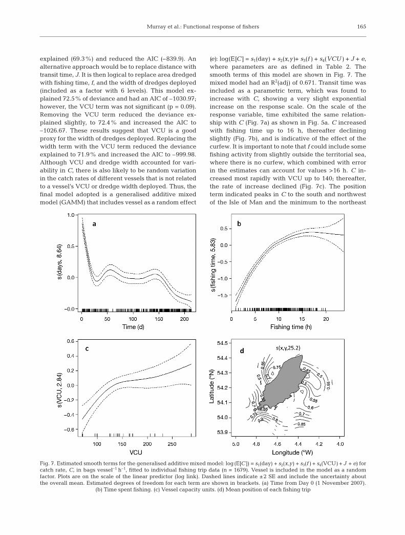
explained (69.3%) and reduced the AIC (–839.9). Analternative approach would be to replace distance withtransit time, J. It is then logical to replace area dredgedwith fishing time, f, and the width of dredges deployed(included as a factor with 6 levels). This model ex -plained 72.5% of deviance and had an AIC of –1030.97;however, the VCU term was not significant (p = 0.09).Removing the VCU term reduced the deviance ex -plained slightly, to 72.4% and increased the AIC to–1026.67. These results suggest that VCU is a goodproxy for the width of dredges deployed. Replacing thewidth term with the VCU term reduced the devianceexplained to 71.9% and increased the AIC to –999.98.Although VCU and dredge width accounted for vari-ability in C, there is also likely to be random variationin the catch rates of different vessels that is not relatedto a vessel’s VCU or dredge width deployed. Thus, thefinal model adopted is a generalised additive mixedmodel (GAMM) that includes vessel as a random effect

(e): log(E[C] = s1(day) + s2(x,y)+ s3(f ) + s4(VCU) + J + e ,where parameters are as defined in Table 2. Thesmooth terms of this model are shown in Fig. 7. Themixed model had an R2(adj) of 0.671. Transit time wasincluded as a parametric term, which was found toincrease with C, showing a very slight exponentialincrease on the response scale. On the scale of theresponse variable, time exhibited the same relation-ship with C (Fig. 7a) as shown in Fig. 5a. C increasedwith fishing time up to 16 h, thereafter decliningslightly (Fig. 7b), and is indicative of the effect of thecurfew. It is important to note that f could include somefishing activity from slightly outside the territorial sea,where there is no curfew, which combined with errorin the estimates can account for values >16 h. C in -creased most rapidly with VCU up to 140; thereafter,the rate of increase declined (Fig. 7c). The positionterm indicated peaks in C to the south and northwestof the Isle of Man and the minimum to the northeast

165

Fig. 7. Estimated smooth terms for the generalised additive mixed model: log(E[C ]) = s1(day) + s2(x,y) + s3(f ) + s4(VCU) + J + e) forcatch rate, C, in bags vessel–1 h–1, fitted to individual fishing trip data (n = 1679). Vessel is included in the model as a random factor. Plots are on the scale of the linear predictor (log link). Dashed lines indicate ±2 SE and include the uncertainty aboutthe overall mean. Estimated degrees of freedom for each term are shown in brackets. (a) Time from Day 0 (1 November 2007).

(b) Time spent fishing. (c) Vessel capacity units. (d) Mean position of each fishing trip

Mar Ecol Prog Ser 430: 157–169, 2011

(Fig. 7d). Whether fishing activity occurred within oroutside the 3 n mile zone had no significant effect (p >0.05) on catch rates. Replacing the time and VCUterms in the mixed model with area dredged reducedthe R2(adj) to 0.645 and increased the AIC from 1198.7to 1378.2.

DISCUSSION

There are 2 fundamental questions that must beanswered to understand fishing behaviour. What influ-ences the spatial and temporal distribution of fishers,and what determines how much fishers catch? Identi-fying the type of functional response fishers exhibitwith changing prey availability can help to answerboth questions, but fishing activity is influenced by anumber of parameters in addition to prey availability.In the present study, we have examined the relation-ship between catch rates and several variables relatingto fishing effort and catchability.

An important consideration when examining thefunctional response of fishers is the index of prey avail-ability used. CPUE is commonly used as an index ofabundance (e.g. Beukers-Stewart et al. 2003, Maunder& Punt 2004) but can also be considered as rate of preyconsumption (e.g. Johnson & Carpenter 1994). Simplyusing mean fleet CPUE does not provide a good indexof abundance, as CPUE may become equalised overfished areas as fishers move to maintain catches (Gilliset al. 1993, Gillis 2003). Therefore, it is essential thatCPUE is standardised to account for the spatial distrib-ution of the fishing fleet (Sampson 1991). Moreover,fishery-dependent estimates of CPUE may be depen-dent on the fleet composition at any given time due tovariability in fishing efficiency between vessels. CPUEis often standardised with reference to a standard vessel for which a long-term record of CPUE is avail-able (Maunder & Punt 2004). However, the catches ofreference vessels may also be altered by the numberof competing vessels and technical advances in com-peting vessels (Rijnsdorp et al. 2008).

CPUE was standardised to account for vessel differ-ences, for which VCUs were found to be a good proxy.VCUs were also found to explain 70 to 80% of the vari-ation in earnings of Scottish trawlers (Pascoe et al.2003). CPUE did broadly parallel the standardisedabundance index. However, there were clear dif -ferences in CPUE between vessels. Moreover, othervariables also influence CPUE. Temperature has a sub-stantial influence on catches of queen scallops Aequi -pecten opercularis, due to their temperature-depen-dent escape response (Jenkins et al. 2003). However,Jenkins & Brand (2001) found no significant effect ofseason on the number of valve adductions in Pecten

maximus following simulated fishing, and there was noclear impact of temperature in the present study. Apotentially important variable not included in thisstudy is that of the abundance of under-sized scallops.Although these are not prey to fishers, in that they arenot targeted and cannot be legally landed, they mayresult in fewer scallops of ≥110 mm being caught. Ifdredges are full, then a greater percentage of under-sized scallops will necessarily result in lower CPUE ofscallops ≥110 mm. Scallop growth stops around De -cember and does not resume until waters warm inMarch, April or May (Mason 1957). Therefore, changesin the size composition of the scallop population due togrowth of scallops will have influenced their catchabil-ity at the end of the fishing season in particular. More-over, it is at this time that the fewest scallops ≥110 mmwere available. Dredges can also be filled with otherbycatch such as brittlestars, or rocks. These variablesmay alter the functional response. In particular, thebasic functional response equations assume that preyavailability, N, and handling time per prey item, t,remain constant during time, T, which in most cases isnot true (Hassell et al. 1976, 1977). The meat yield ofscallops will also affect their value. High-grading is notthought to occur in the scallop fishery; smaller scallopsover the minimum landing size could be discarded infavour of larger, more valuable scallops. However,there would be no advantage to fishers in doing sounless the vessel was nearing maximum catch capac-ity, which did not appear to occur.

The importance of distinguishing between the formsof functional response is that a type II or III responseindicates density-dependent catchability, compared todensity independence in a type I response (Egglestonet al. 2008). Furthermore, a type III response can stabilise prey populations (Hassell & Comins 1978,Nunney 1980, Nachman 2006). However, predator–prey populations do not always conform to a singleresponse type (Jeschke et al. 2004). The results of ourstudy indicate that the functional response of the fish-ing fleet did not conform to one particular type and thatprey density was not high enough for prey consump-tion to reach a plateau. Therefore, the fishery was notat saturation, with vessels still able to exploit the high-est abundance of scallops. It is important to note thatalmost all values of abundance >40 occurred withinthe first month of fishing, indicating that abundancewas depleted rapidly. Fishers’ knowledge of scallopdistribution may have been greater after the firstmonth of fishing, allowing them to exploit higher-density patches of scallops to maintain catches. There-after, prey consump tion rates may have been reducedas prey became increasingly patchy (Essington et al.2000) towards the end of the fishing season when mostareas had been fished. Given that fishers cannot have

166

Murray et al.: Functional response of fishers

perfect knowledge of the distribution of scallop popu-lations, the chance of a fisher encountering patchesof scallops must be reduced at the end of the fishingseason.

Previous catch rates are a major influence on thechoice of fishing location (Hutton et al. 2004). In thescallop fishery, catches of under-sized scallops in theprevious season will provide a good predictor ofcatches in the following season (Beukers-Stewart et al.2003) and where fishers have knowledge of areas withhigh CPUE, they are likely to target them (Dreyfus-León 1999). All of the fishing activity observed in thepresent study corresponds with historically recognisedscallop fishing grounds (Beukers-Stewart et al. 2003).Thus, fishers clearly had some knowledge of the distri-bution of scallop populations. However, in the scallopfishery, fishing has to be undertaken before CPUE canbe determined, unlike other fisheries where sonarcan be utilised (e.g. Brehmer et al. 2007, Boswell et al.2008). Therefore, knowledge of prey distribution willnecessarily be imperfect, limiting the numerical re -sponse. Moreover, interference competition may pre-vent fishing in optimal areas (Rijnsdorp et al. 2000a,b).Catches were not obviously suppressed by interfer-ence competition in the present study; however, highscallop abundance could mask competitive interac-tions. Nevertheless, both the number of vessels fishingand catches were highest at the beginning of the season. It is also possible that fishers exerted greaterfishing effort when competition was greater.

The rate of deceleration in consumption rates athigher prey densities cannot be predicted; however, itis likely there would be a sharp deceleration either dueto satiation (no market demand) or vessels filling theirholds to capacity, and the result may be a type I/IIIresponse, as described by Jeschke et al. (2004). Type Ifunctional responses have only been reported in filterfeeders (Jeschke et al. 2004), while type III responsesare often exhibited by generalist predators that canswitch between prey species (Van Leeuwen et al. 2007,Kempf et al. 2008). Although scallop dredgers maytake bycatch, such as Aequipecten opercularis, the Isleof Man scallop fleet targeted only great scallops duringthis open scallop fishing season, with queen scallopsconstituting a very small proportion of total landings,amounting to around 5 t from all vessels during thegreat scallop fishing season.

It may be possible to refine the analysis of the dataused in this study. For example, improved estimates offishing time may be achieved by adopting methods toreconstruct trawl tracks. Hintzen et al. (2010) used aspline interpolation technique to model fishing tracksfrom VMS data while Vermard et al. (2010) identifieddifferent fishing behaviour during fishing trips, usingBayesian hierarchical models. Moreover, the collection

of additional data such as individual tow length andcatches per tow would allow more detailed analysis ofhow fishers respond to changing prey availability.Nevertheless, several conclusions can be drawn fromour study.

The assumptions of Holling’s disc equation were notappropriate in the Isle of Man scallop fishery. Further-more, the functional response did not conform verywell to a particular type. The increasing patchinessof scallops towards the end of the season probablyreduced their catchability, but fishers were able tomaintain catch rates at intermediate abundance levels,suggesting knowledge of prey distribution. An impor-tant aspect of the observed functional response is thatthere is latent capacity in the fishing fleet. Eggleston etal. (2003, 2008) observed a type I response in a non-saturated Panulirus argus fishery and therefore con-cluded that reducing catch limits would be the mosteffective means of reducing landings. Similarly, settingcatch limits or reducing vessels’ fishing power togetherwith a reduction in vessel numbers would result ina greater reduction in scallop landings at the highestprey densities, while limiting vessel numbers alonemay have little impact. Incorporating additional vari-ables, especially the size composition of scallop popu-lations, into the models presented here will help to further elucidate the relationship between scallop fishers and their prey.

Acknowledgements. This work was funded by the Isle of ManGovernment Department of Environment, Food and Agricul-ture, to whom we are grateful; we especially thank A. Readand J. Eaton. Thanks also to W. Caley for providing dataon scallop landings. We are also grateful to the Met Officefor providing data from the UK wave model, and to the anonymous reviewers whose comments greatly improved themanuscript.

LITERATURE CITED

Abrams PA (1982) Functional responses of optimal foragers.Am Nat 120:382–390

Babcock EA, Pikitch EK (2000) A dynamic programmingmodel of fishing strategy choice in a multispecies trawlfishery with trip limits. Can J Fish Aquat Sci 57:357–370

Beckerman S (1983) Optimal foraging group-size for a human-population—the case of Bari fishing. Am Zool 23: 283–290

Begossi A (1992) The use of optimal foraging theory in theunderstanding of fishing strategies—a case from SepetibaBay (Rio De Janeiro State, Brazil). Hum Ecol 20:463–475

Béné C, Tewfik A (2001) Fishing effort allocation and fisher-men’s decision making process in a multi-species small-scale fishery: analysis of the conch and lobster fishery inTurks and Caicos Islands. Hum Ecol 29:157–186

Beukers-Stewart BD, Mosley MWJ, Brand AR (2003) Popula-tion dynamics and predictions in the Isle of Man fisheryfor the great scallop (Pecten maximus, L.). ICES J Mar Sci60:224–242

Beukers-Stewart BD, Vause BJ, Mosley MWJ, Rossetti HL,

167

Mar Ecol Prog Ser 430: 157–169, 2011

Brand AR (2005) Benefits of closed area protection for apopulation of scallops. Mar Ecol Prog Ser 298:189–204

Boswell KM, Wilson MP, Cowan JH (2008) A semiautomatedapproach to estimating fish size, abundance, and behaviorfrom dual-frequency identification sonar (DIDSON) data.N Am J Fish Manag 28:799–807

Brehmer P, Georgakarakos S, Josse E, Trygonis V, Dalen J(2007) Adaptation of fisheries sonar for monitoring schoolsof large pelagic fish: dependence of schooling behaviouron fish finding efficiency. Aquat Living Resour 20:377–384

Caldow RWG, Furness RW (2001) Does Holling’s disc equa-tion explain the functional response of a kleptoparasite?J Anim Ecol 70:650–662

Crawley MJ (2007) The R book. Wiley-Blackwell, ChichesterDreyfus-León MJ (1999) Individual-based modelling of fisher-

men search behaviour with neural networks and rein-forcement learning. Ecol Model 120:287–297

Eggleston DB, Johnson EG, Kellison GT, Nadeau DA (2003)Intense removal and non-saturating functional responsesby recreational divers on spiny lobster Panulirus argus.Mar Ecol Prog Ser 257:197–207

Eggleston DB, Parsons DM, Kellison GT, Plaia GR, JohnsonEG (2008) Functional response of sport divers to lobsterswith application to fisheries management. Ecol Appl 18:258–272

Essington TE, Hodgson JR, Kitchell JF (2000) Role of satiationin the functional response of a piscivore, largemouth bass(Micropterus salmoides). Can J Fish Aquat Sci 57:548–556

Gascoigne JC, Lipcius RN (2004) Allee effects driven by pre-dation. J Appl Ecol 41:801–810

Gerritsen H, Lordan C (2011) Integrating vessel monitoringsystems (VMS) data with daily catch data from logbooks toexplore the spatial distribution of catch and effort at highresolution. ICES J Mar Sci 68:245–252

Gillis DM (2003) Ideal free distributions in fleet dynamics: abehavioral perspective on vessel movement in fisheriesanalysis. Can J Zool 81:177–187

Gillis DM, Peterman RM, Tyler AV (1993) Movement dynam-ics in a fishery—application of the ideal free distributionto spatial allocation of effort. Can J Fish Aquat Sci 50:323–333

Gillis DM, Pikitch EK, Peterman RM (1995) Dynamic discard-ing decisions—foraging theory for high-grading in a trawlfishery. Behav Ecol 6:146–154

Griffen BD (2009) Consumers that are not ‘ideal’ or ‘free’ canstill approach the ideal free distribution using simplepatch-leaving rules. J Anim Ecol 78:919–927

Hassell MP, Comins HN (1978) Sigmoid functional responsesand population stability. Theor Popul Biol 14:62–67

Hassell MP, Lawton JH, Beddington JR (1976) Componentsof arthropod predation. 1. Prey death-rate. J Anim Ecol 45:135–164

Hassell MP, Lawton JH, Beddington JR (1977) Sigmoid func-tional responses by invertebrate predators and para-sitoids. J Anim Ecol 46:249–262

Hintzen NT, Piet GJ, Brunel T (2010) Improved estimation oftrawling tracks using cubic Hermite spline interpolationof position registration data. Fish Res 101:108–115

Holling CS (1959) Some characteristics of simple types of predation and parasitism. Can Entomol 91:163–182

Holling CS (1961) Principles of insect predation. Annu RevEntomol 6:163–182

Höner OP, Wachter B, East ML, Hofer H (2002) The responseof spotted hyaenas to long-term changes in prey popula-tions: functional response and interspecific kleptopara-sitism. J Anim Ecol 71:236–246

Hutton T, Mardle S, Pascoe S, Clark RA (2004) Modelling fish-

ing location choice within mixed fisheries: English NorthSea beam trawlers in 2000 and 2001. ICES J Mar Sci61:1443–1452

Isle of Man Government Laboratory (2007) Marine monitor-ing 2007. Isle of Man Government, Isle of Man

Isle of Man Government Laboratory (2008) Marine monitor-ing summary 2008. Isle of Man Government, Isle of Man

Jaksic FM, Jimenez JE, Castro SA, Feinsinger P (1992)Numerical and functional response of predators to a long-term decline in mammalian prey at a semiarid neotropicalsite. Oecologia 89:90–101

Jenkins SR, Brand AR (2001) The effect of dredge capture onthe escape response of the great scallop, Pecten maximus(L.): implications for the survival of undersized discards.J Exp Mar Biol Ecol 266:33–50

Jenkins SR, Lart W, Vause BJ, Brand AR (2003) Seasonalswimming behaviour in the queen scallop (Aequipectenopercularis) and its effect on dredge fisheries. J Exp MarBiol Ecol 289:163–179

Jeschke JM, Kopp M, Tollrian R (2002) Predator functionalresponses: discriminating between handling and digest-ing prey. Ecol Monogr 72:95–112

Jeschke JM, Kopp M, Tollrian R (2004) Consumer-food sys-tems: why type I functional responses are exclusive to filter feeders. Biol Rev Camb Philos Soc 79:337–349

Johnson BM, Carpenter SR (1994) Functional and numericalresponses: a framework for fish-angler interactions? EcolAppl 4:808–821

Kempf A, Floeter J, Temming A (2008) Predator–prey overlap-induced Holling type III functional response in the NorthSea fish assemblage. Mar Ecol Prog Ser 367:295–308

Kim YJ, Gu C (2004) Smoothing spline Gaussian regression:more scalable computation via efficient approximation.J R Stat Soc Ser B Stat Methodol 66:337–356

Lee J, South AB, Jennings S (2010) Developing reliable,repeatable, and accessible methods to provide high-resolution estimates of fishing-effort distributions fromvessel monitoring system (VMS) data. ICES J Mar Sci 67:1260–1271

Mason J (1957) The age and growth of the scallop, Pectenmaximus (L), in Manx waters. J Mar Biol Assoc UK 36:473–492

Maunder MN, Punt AE (2004) Standardizing catch and effortdata: a review of recent approaches. Fish Res 70:141–159

Met Office (2009) UK waters wave model. Met Office, Exeter Mills CM, Townsend SE, Jennings S, Eastwood PD, Houghton

CA (2007) Estimating high resolution trawl fishing effortfrom satellite-based vessel monitoring system data. ICES JMar Sci 64:248–255

Nachman G (2006) A functional response model of a predatorpopulation foraging in a patchy habitat. J Anim Ecol 75:948–958

Nunney L (1980) The influence of the type-3 (sigmoid) func-tional-response upon the stability of predator-prey differ-ence models. Theor Popul Biol 18:257–278

Pascoe S, Kirkley JE, Greboval D, Morrison-Paul CJ (2003)Measuring and assessing capacity in fisheries. 2. Issuesand methods. FAO Fish Tech Pap 433/2. FAO, Rome

Poos JJ, Bogaards JA, Quirijns FJ, Gillis DM, Rijnsdorp AD(2010) Individual quotas, fishing effort allocation, andover-quota discarding in mixed fisheries. ICES J Mar Sci67:323–333

Real LA (1977) Kinetics of functional response. Am Nat 111:289–300

Rijnsdorp AD, Dol W, Hoyer M, Pastoors MA (2000a) Effectsof fishing power and competitive interactions among ves-sels on the effort allocation on the trip level of the Dutch

168

Murray et al.: Functional response of fishers 169

beam trawl fleet. ICES J Mar Sci 57:927–937Rijnsdorp AD, Broekman PLV, Visser EG (2000b) Competitive

interactions among beam trawlers exploiting local patchesof flatfish in the North Sea. ICES J Mar Sci 57:894–902

Rijnsdorp AD, Poos JJ, Quirijns FJ, Hille Ris Lambers R, WildeJWD, Heijer WMD (2008) The arms race between fishers.J Sea Res 60:126–138

Sampson DB (1991) Fishing tactics and fish abundance, andtheir influence on catch rates. ICES J Mar Sci 48:291–301

Shephard S, Beukers-Stewart B, Hiddink JG, Brand AR,Kaiser MJ (2009) Strengthening recruitment of exploitedscallops Pecten maximus with ocean warming. Mar Biol157:91–97

Smout S, Asseburg C, Matthiopoulos J, Fernandez C, Red-path S, Thirgood S, Harwood J (2010) The functionalresponse of a generalist predator. PLoS ONE 5:e10761

Solomon ME (1949) The natural control of animal popula-tions. J Anim Ecol 18:1–35

Thomas GE, Gruffydd LD (1971) Types of escape reactionselicited in scallop Pecten maximus by selected sea-starspecies. Mar Biol 10:87–93

Van Leeuwen E, Jansen VAA, Bright PW (2007) How popula-tion dynamics shape the functional response in a one-predator-two-prey system. Ecology 88:1571–1581

Vermard Y, Rivot E, Mahevas S, Marchal P, Gascuel D (2010)Identifying fishing trip behaviour and estimating fishingeffort from VMS data using Bayesian Hidden MarkovModels. Ecol Model 221:1757–1769

Wong MC, Barbeau MA (2005) Prey selection and the func-tional response of sea stars (Asterias vulgaris Verrill) androck crabs (Cancer irroratus Say) preying on juvenile seascallops (Placopecten magellanicus (Gmelin)) and bluemussels (Mytilus edulis Linnaeus). J Exp Mar Biol Ecol327:1–21

Wood SN (2006) Generalized additive models: an introductionwith R. Chapman & Hall/CRC, London

Wood SN (2008) Fast stable direct fitting and smoothnessselection for generalized additive models. J R Stat Soc SerB Stat Methodol 70:495–518

Wood SN, Augustin NH (2002) GAMs with integrated modelselection using penalized regression splines and applica-tions to environmental modelling. Ecol Model 157:157–177

Submitted: April 27, 2010; Accepted: January 31, 2011 Proofs received from author(s): March 25, 2011