Functional Magnetic Resonance Imaging:Methods and Applications

Stuart Clare

Submitted to the University of Nottinghamfor the degree of Doctor of Philosophy

October 1997

email: stuart@fmrib.ox.ac.ukweb: http://www.fmrib.ox.ac.uk/~stuart

AbstractThe technique of functional magnetic resonance imaging is rapidly moving from one of technicalinterest to wide clinical application. However, there are a number of questions regarding the methodthat need resolution. Some of these are investigated in this thesis.

High resolution fMRI is demonstrated at 3.0 T, using an interleaved echo planar imaging technique tokeep image distortion low. The optimum echo time to use in fMRI experiments is investigated using amultiple gradient echo sequence to obtain six images, each with a different echo time, from a singlefree induction decay. The same data are used to construct T2

* maps during functional stimulation.

Various techniques for correcting the N/2 ghost are tested for use in fMRI experiments, and a methodfor removing the image artefact caused by external r.f. interference in a non-linearly sampled matrix ispresented.

The steps in the analysis of fMRI data are detailed, and two new non-directed analysis techniques,particularly for data from single events, as opposed to epoch based paradigms, are proposed. Thetheory behind software that has been written for fMRI data analysis is also given.

Finally, some of the results from an fMRI study into the initiation of movement are presented,illustrating the power of single event experiments in the separation of cognitive processes.

AcknowledgementsI would like to thank my supervisors, Prof. Peter Morris and Dr. Richard Bowtell, for the support andadvice they have provided throughout the duration of my Ph.D. I am also indebted to Dr. Jon Hykinfor teaching me the art of functional MRI and to Dr. Miles Humberstone for providing the impetus formuch of my work. I would also like to thank all the people with whom I have worked over the pastthree years without whom none of this work could have been done, and particularly those who havepatiently laid in the scanner for my experiments. Finally I would like to thank the University ofNottingham for their funding.

Chapter 1 - Introduction

1.1 Probing the Secrets of the Brain

The brain is the most fascinating, and least understood, organ in the human body. For centuries,scientists and philosophers have pondered the relationship between behaviour, emotion, memory,thought, consciousness, and the physical body. In the Middle Ages there was much controversy as towhether the soul was located in the brain or in the heart. As ideas developed however, it was suggestedthat mental processes were located in the ventricles of the brain. According to this theory ’commonsense’ was located in the lateral ventricles, along with imagination accommodated in the posterior part.The third ventricle was the seat of reasoning, judgement and thought, whilst memory was contained inthe fourth ventricle.

It was in the 17th century that Thomas Willis proposed that various areas of the cortex of the brain hadspecific functions, in particular the circle of vessels at the base of the brain which now bear his name.In the 19th century, Gall put forward his ’science’ of phrenology, where the presence or absence ofbumps on the skull revealed the strength or weakness of various mental and moral faculties. Despitethe dubious method he used, Gall put forward two very important concepts: that the brain was the seatof all intellectual and moral faculties; and that particular activities could be localised to some specificregion of the cerebral cortex.

The study of brain function progressed in the late 19th century through work involving the stimulationof the cortex of animal brains using electrical currents. This lead to the mapping of motor function inanimals and, later, in humans. These results however contained many inconsistencies. More reliablework was carried out in the mid 20th century by Penfield, who managed to map the motor andsomatosensory cortex using cortical stimulation of patients undergoing neurosurgery. In the latter halfof this century, most progress in the study of brain function has come from patients with neurologicaldisorders or from electrode measurements on animals. It has only been in the last decade or so thatbrain imaging techniques have allowed the study of healthy human subjects.

1.2 Pictures of the Mind

The impact of medical imaging on the field of neuroscience has been considerable. The advent ofx-ray computed tomography (CT) in the 1970’s allowed clinicians to see features inside the heads ofpatients without the need for surgery. By making the small step of placing the source of radiationwithin the patient, x-ray CT became autoradiography, so that now not only structure but also bloodflow and metabolism could be followed in a relatively non-invasive way. A big step forward was madeby choosing to use a positron emitter as the radioisotope. Since a positron almost immediatelyannihilates with an electron, emitting two photons at 180 degrees to each other, much betterlocalisation of the radioisotope within the scanner is obtained. Using labelled water, positron emissiontomography (PET) became the first useful technique which allowed researchers to produce maps of themind, by measuring blood flow during execution of simple cognitive tasks. Since local blood flow isintimately related to cortical activity, regions of high regional blood flow indicate the area in thecortex responsible for the task being performed.

At around the same time, another technique which promised even better anatomical pictures of thebrain was being developed. Magnetic resonance imaging (MRI), based on the phenomenon of nuclearmagnetic resonance, produces images of the human body with excellent soft tissue contrast, allowingneurologists to distinguish between grey and white matter, and brain defects such as tumours. SinceMRI involves no ionising radiation, the risks to the subject are minimised. The development of

contrast agents suitable for dynamic MRI studies, and improvements in the speed of imaging, openedup the possibility of using the technique for functional brain studies. In 1991 the first experiment usingMRI to study brain function was performed, imaging the visual cortex whilst the subject was presentedwith a visual stimulus. A contrast agent was used in this first study, but it was not much later when thefirst experiment was carried out using the blood as an endogenous contrast agent. The haemoglobin inthe blood has different magnetic properties depending on whether it is oxygenated or not; thesedifferences affect the signal recorded in the MR image. By imaging a subject at rest and whilstcarrying out a specific task, it became possible to image brain function in a completely non-invasiveway.

The ’pictures of the mind’ that have been produced over the past few years have started to make a bigimpact on the way neuroscience is approached. There are, however, still areas of the technique offunctional MRI that require refinement. The fast imaging method of echo planar imaging, which isessential for fast dynamic studies, can suffer from poor image quality. In addition some areas of thebrain are not visible on its scans. The mechanisms behind the observed activation response are notwell understood, and there are issues involved in the way that the data from such experiments areanalysed. However, the potential of fMRI, alongside that of PET, means that the study of the humanbrain has entered a new era, offering new insights into neurology, psychiatry, psychology and perhapseven contributing to the philosophical debate about the relationship between mind and brain.

1.3 The Scope of this Thesis

The material presented in this thesis covers a number of the aspects concerning the technique andapplication of functional MRI.

The second chapter covers the theory of magnetic resonance imaging, including the classical andquantum mechanical descriptions of nuclear magnetic resonance, and the variety of techniques that canbe used to image biological samples. The origin of contrast in MRI is then described and the sourcesof image artefacts discussed. The chapter ends with two sections on practical imaging, one on thehardware that is required for MRI and another on the safety aspects of putting human volunteers insideMR scanners.

Chapter Three is concerned primarily with brain function. An outline of the main techniques used forfunctional neuroimaging, including positron emission tomography, magnetoencephalography andmagnetic resonance spectroscopy, is given. Some basic aspects of neuroscience are then covered, andthe main structures in the brain, its biochemistry and functional organisation are described. Thetechnique of fMRI is covered in detail, describing how brain activity affects the contrast in the MRimage, how experiments are performed and how the data are analysed.

The three chapters that follow cover improvements in the technique of fMRI. Chapter Four deals withthe optimisation of MRI for functional brain imaging. Experiments that determine the optimum imageecho time (TE) to use in an fMRI study are described. These use a technique that acquires six images,each with a different echo time, in a single shot. The reduction of image artefact is the subject of thenext section. A number of post-processing techniques that reduce the Nyquist or N/2 ghost arecompared for effectiveness on fMRI data sets and a method for removing the bands on images thatresult from external r.f. interference is demonstrated. Finally in this chapter, a technique for the fastacquisition of inversion recovery anatomical reference scans is described.

The implementation of the technique of interleaved echo planar imaging is the subject of the fifthchapter. The reasons for using the technique are explained, and the problems that have arisen in its usefor high resolution, low distortion fMRI are discussed. Chapter Six covers aspects relating to the

analysis of fMRI data to produce statistically robust results. The theory and implementation of anumber of image pre-processing techniques is described and the statistical techniques that can be usedto detect regions of activation are outlined. Two new statistical analysis methods are described, both ofwhich make no assumptions as to the shape of the activation response that is expected. The theorybehind software that is used to draw inference from the resulting statistics is explained and ways ofpresenting the final data are described.

Chapter Seven presents the results from an fMRI study of motor function in normal volunteers andpatients with Parkinson’s disease. Aspects of the stimulus paradigm design and implementation arecovered, as is the optimisation of the imaging and experimental protocol.

1.4 References

The material on the history of the study of brain function comes from:

Clarke, E. and Dewhurst, K. (1972) ’An Illustrated History of Brain Function’, SandfordPublications, Oxford.

Detailed references on the history of PET and fMRI are given in Chapter 3, however basicintroductions to these topics are given in:

Ter-Pogossian, M. M., Raichle, M. E. and Sobel, B. E. Positron Emission Tomography. Scientific American October 1980. Pykett, I. L. NMR Imaging in Medicine. Scientific American May 1982. Raichle, M. E. Visualizing the Mind. Scientific American April 1994.

Chapter 2 - Principles of Magnetic Resonance Imaging

2.1 Introduction

The property of Nuclear Magnetic Resonance (NMR) was first described by Purcell [1] and Bloch [2]in 1946, work for which they received the Nobel prize in 1952. Since then NMR has become apowerful tool in the analysis of chemical composition and structure. In 1973 Lauterbur [3] andMansfield [4] used the principles of NMR to describe a technique for determining physical structure.Since then Magnetic Resonance Imaging (MRI) has been used in many biomedical, chemical andengineering applications.

In this chapter the theoretical foundations, first of nuclear magnetic resonance and then magneticresonance imaging are explained. Then the practical implementation of MRI is outlined, and anexplanation of the artefacts that affect MR images given. The chapter ends with a discussion of thesafety of MRI as a medical imaging modality. This chapter serves only as an outline of the basicprinciples of nuclear magnetic resonance spectroscopy and imaging. More detail is found in thestandard texts on the subject, such as those by Abragamm [5], and Callaghan [6].

2.2 Nuclear Magnetic Resonance

2.2.1 The Quantum Mechanical Description of NMR

The quantum mechanical description of atomic nuclei, as described by Dirac in 1930, predicted theproperty of spin angular momentum. In fact the property of electron spin was observed six yearsearlier by Stern and Gerlach [7], who passed a beam of neutral atoms through a non-uniform magneticfield, and observed the effect of half-integral angular momentum, that could not be explained by thepreviously accepted Bohr model.

This spin angular momentum is characterised by the spin quantum number I, such that the total spinangular momentum is Ih. The value of I is an intrinsic property of the nucleus, examples of which aregiven in Table 2.1.

NucleusSpin Quantum Number

I

1H 1/2

2H 1

12C 0

13C 1/2

19F 1/2

31P 1/2

Table 2.1 Spin quantum numbers for some atomic nuclei

To exhibit the property of magnetic resonance the nucleus must have a non-zero value of I. As far asmedical applications are concerned, the proton (1H) is the nucleus of most interest, because of its highnatural abundance. However, other nuclei have been studied, most noticeably 13C whose low naturalabundance relative to 12C makes it suitable for tracer studies.

The magnitude of the spin angular momentum is given by

(2.1)

but since P is a vector, its orientation must be taken into account. In a magnetic field, applied along thez axis, the possible values of the z-components of the angular momentum are given by

where

.

(2.2)

So for the proton, with spin 1/2, there are two possible values for , that is . The

eigenfunction describing the spin state of the proton nucleus can be written as or , andsince in quantum mechanics every physical observable has an associated operator, we can write aneigenvalue equation to describe the observation of the spin state as

(2.3)

where is the operator describing measurement of the angular momentum along the z axis. There aresimilar operators for measuring the angular momentum along the x and y axes, so we have a range ofeigenvalue equations for a spin 1/2 system as follows:

(2.4)

To measure the energy of the spin system it is necessary to construct a Hamiltonian operator. The formof the Hamiltonian can be derived from classical electromagnetism for the energy of a magneticmoment placed in a magnetic field.

Nuclei have a magnetic moment, m, which is proportional to the angular momentum,

(2.5)

Nuclei with the constant of proportionality, g, being called the magnetogyric ratio. The magnetogyricratio is a property of the particular nucleus, and has a value of 2.675 x 10 8 rad/s/T for protons. When

this magnetic moment is placed in a magnetic field, B, it has energy

(2.6)

and so by combining equations 2.5 and 2.6 a Hamiltonian can be defined as

.

(2.7)

Since by definition the B field is applied parallel to the z-axis the Hamiltonian becomes

(2.8)

and is known as the Zeeman Hamiltonian. Now using the Schrödinger equation, the energy of theeigenstate is found.

(2.9)

So for a proton with , a transition between the two states represents a change in energy

(2.10)

Figure 2.1 Energy level diagram for a proton under the Zeeman interaction.

This is called the Zeeman splitting, and is shown as an energy level diagram in Figure 2.1. These twostates are given a variety of labels, but most commonly referred to as ’spin up’, and ’spin down’, withthe spin-down state having a higher energy than the spin-up state. Transitions between the two statescan be induced by absorption or emission of a photon of frequency n 0, such that

(2.11)

Expressing the frequency in angular terms gives the Larmor equation which underpins the whole ofNMR

(2.12)

the characteristic frequency, w, being the Larmor frequency. The magnetic field, labelled B0, is still

assumed to be applied along the z axis, and is now subscripted with a ’0’ to distinguish it from theapplied radio frequency field which will be introduced later.

This description of the quantum mechanical behaviour of an atomic nucleus leads to the way NMR isperformed. Transitions between the two energy states, spin-up and spin-down, can occur by absorptionor emission of electromagnetic radiation of frequency given by the Larmor equation. This frequencydepends, for a given species of nuclei, purely on the applied magnetic field. It is the strength of thefield experienced by the nucleus that enables structure to be determined in spectroscopy experiments,and position to be found in imaging experiments.

In a real system there is not just one nucleus in isolation, but many nuclei all of which could occupy aparticular spin state. This means that the theory must be extended to consider an ensemble of spins.

To do this a single eigenstate Y, which is a linear combination of the possible spin states for a singlenucleus is defined

(2.13)

When making a measurement on such a system, the expectation value of the operation on thissuperposition of states is

(2.14)

where the value represents the probability of finding a single nucleus in the state mI . So for the

case of a proton, with two spin states

(2.15)

The ratio of the populations of the two energy states from Boltzman statistics is

(2.16)

so the difference between the number of spins in the spin-up state and the spin-down state is

(2.17)

If we now assume that all the ’spin up’ nuclei have a magnetic moment of and the ’spin down’

nuclei have a magnetic moment of - , then we can write the bulk magnetisation of the ensembleas

(2.18)

where N is the number of spins in the ensemble. Being able to treat the behaviour of all the spins in thesystem in terms of magnetisation allows a transfer from a quantum mechanical to a classicaldescription of NMR. The advantage of the classical description is that it gives a simpler picture of theNMR experiment.

2.2.2 The Classical Description of NMR

If the spin magnetisation vector M is placed in a magnetic field B, M will experience a torque. Theequation of motion for M can be written

.

(2.19)

If B is a static (time-independent) field along the z axis such that then equation 2.19becomes

(2.20)

which has solutions

(2.21)

where . These equations describe the precession of the magnetisation vector about the z axisas shown in Figure 2.2. The angular frequency of the precession is identical to the Larmor frequencyderived in the quantum mechanical description above (equation 2.12), showing how the classical andquantum mechanical pictures coincide.

Figure 2.2 Precession of the magnetisation vector in a static magnetic field aligned along the z-axis.

Now, as well as the static B0 field applied along z, consider a time varying field B1 , applied

perpendicularly to B0 and oscillating at w0. If only the circularly polarised component of B1 rotating

in the same direction as the precessing magnetisation vector is considered

(2.22)

which when put into equation 2.19 yields

(2.23)

If a starting condition M (0)=M0k is defined, then the solutions for M are

(2.24)

where .

This implies that by applying an oscillating magnetic field of frequency w0, the magnetisation

simultaneously precesses about B0 at w 0 and B1 at w 1, as shown in Figure 2.3a.

At this point it is appropriate to introduce a new frame of reference for viewing the evolution of themagnetisation vector, the rotating frame, which rotates about the z-axis at frequency w 0. If in the

rotating frame an axis system (x’,y’,z) is defined then equation 2.19 can be written

(2.25)

where

(2.26)

and (i’,j’,k ) are unit vectors in the (x’,y’,z) directions. The result of solving these two equations is amagnetisation vector which precesses about Beff , as shown in Figure 2.3b. If

and M precesses about the x’ axis shown in Figure 2.3c. Applying the B 1 field has the effect of rotating the magnetisation vector about the x’-axis at an angular frequency

w1= g B1.

(a)

(b)

(c)Figure 2.3 Precession of magnetisation (a) in the laboratory frame under the influence of

longitudinal field B 0 , and transverse field B1 , (b) in the rotating frame under the influence offield B eff and (c) in the rotating frame when B0 =w/g.

The most common way to carry out an NMR experiment is to apply a short burst of resonant r.f. field.

If the duration of this r.f. pulse is t, then the magnetisation will rotate by an angle . If thatangle is 90 degrees then the pulse is referred to as a 90x pulse, the x subscript showing that the

precession is about the x’ axis. In a typical NMR experiment a 90x pulse is applied, which tips the

magnetisation vector from the longitudinal plane (parallel to B0) to the transverse plane

(perpendicular to B0). Once in the transverse plane the magnetisation can be detected as it precesses

about the z-axis, and this is what gives rise to the NMR signal, which is discussed in the next section.

2.2.3 Relaxation and Signal Detection

Since the application of a resonant r.f. pulse disturbs the spin system, there must subsequently be aprocess of coming back to equilibrium. This involves exchange of energy between the spin system andits surroundings. Such a process is called spin-lattice relaxation, and the rate at which equilibrium isrestored is characterised by the spin-lattice or longitudinal relaxation time, T1, in a new equation of

motion for Mz

(2.27)

The spins however do not only exchange energy with the surrounding lattice, but also amongthemselves. This is generally a faster process than spin-lattice relaxation, and is characterised by thespin-spin relaxation time, T2, in the equations describing the evolution of Mx and My

.

(2.28)

Equations 2.27 and 2.28, when combined with the earlier equations of motion form what are known asthe Bloch equations

(2.29)

given here for the rotating frame of reference.

Immediately following the application of a Qx pulse, the magnetisation vector has components

which when put in the Bloch equations give

.

(2.30)

The relaxation times T1 and T2 are very important in imaging, as they have the greatest effect in

determining contrast.

Figure 2.4 Orientation of the r.f. coil within the static field.

To detect the NMR signal it is necessary to have an r.f. coil which is in the transverse plane, that isperpendicular to the B0 field (Figure 2.4), in which an e.m.f. is induced which is proportional to Mx .

The signal from the coil is first transformed to the rotating frame by phase sensitive detection.Normally this involves separately mixing the e.m.f. with two reference signals, both oscillating at theLarmor frequency, but 90 degrees out of phase with each other. Thus the signal detected in the coil hasthe form

(2.31)

which after phase sensitive detection has ’real’ and ’imaginary’ components

(2.32)

where D=w-w0. If w=w0 then the signal is just an exponential decay, however if w≠w0 then the

signal will oscillate at a frequency D. The signal after phase sensitive detection is known as the FreeInduction Decay (FID). Fourier transformation of the FID gives the value of D as shown in Figure 2.5.The width of the peak is governed by T2. This relationship is explored further in Chapter 5.

Figure 2.5 The ’real’ and imaginary component of the FID and its Fourier transform for (a)resonance signal and (b) off-resonance signal.

A summary of the theory of NMR as presented so far under a classical description is that, a staticmagnetic field, B0, polarises the sample such that it has a bulk magnetisation aligned with the

direction of the field. An oscillating magnetic field at the Larmor frequency applied for a short timeorthogonally to B0 will cause the longitudinal magnetisation to be tipped into the transverse plane.

This makes the Larmor precession of the magnetisation under B0 detectable, and Fourier

transformation of the phase sensitively detected signal yields its offset from the expected value.

It is this offset from expected value that is most useful in magnetic resonance, as the B0 field

experienced by the different spins in the system is sensitive to nature of the chemical environment andcan be manipulated by the application of external magnetic field gradients. The former is exploited inMagnetic Resonance Spectroscopy (MRS) and the latter in Magnetic Resonance Imaging.

2.2.4 Chemical Shift and Magnetic Resonance Spectroscopy

The electrons that surround each nucleus can act to slightly perturb the magnetic field at the spin site.This causes the Larmor precession frequency to be modified by the chemical environment of the spin.The effect of chemical shift is described by the equation

(2.33)

where s is the shielding constant. This modifies the Larmor frequency such that

(2.34)

and is detected upon Fourier transformation of the FID as a shift in frequency away from that expectedif chemical shift played no part. For a sample containing spins with a number of different chemicalshifts, the resulting spread of frequencies represents a chemical spectrum. An example of an NMRspectrum is shown in Figure 2.6.

Figure 2.6 A 13C spectrum of human muscle acquired in vivo at 3.0 Tesla

It is common to express the chemical shift of a peak in the spectrum in terms of the relative differencein frequency from some reference peak. The chemical shift in parts per million (p.p.m.) is thereforedefined as

(2.35)

where n and nref are the resonant frequencies of the spectral peak of interest and the reference

component respectively. Chemical shifts in 1H spectra are of the order of a few p.p.m.

Another spin effect that is useful in MRS is the scalar, or spin-spin coupling. This arises frominteractions between the nuclear spins, mediated by the delocalised electrons. However this effect isnot very important in imaging, since its magnitude is so small. There are a number of other features ofspin behaviour which affect the NMR signal. Some of these will be described, where appropriate, inother chapters.

2.3 Magnetic Resonance Imaging

2.3.1 Magnetic Field Gradients

As has been shown in Section 2.2, the fundamental equation of magnetic resonance is the Larmor

equation, . In an NMR experiment a measurement of the frequency of precession of themagnetisation gives information on the field experienced by that group of spins. By manipulating thespatial variation of the field in a known way, this frequency information now yields spatialinformation.

Consider a linear field gradient in B which increases along the x axis, such that

(2.36)

where G is the gradient strength. This makes the Larmor equation

(2.37)

or in its more general three dimensional form

(2.38)

Under a linear field gradient along the x axis, all the spins which lie at a particular value of x willprecess at the same frequency. The FID from such a sample will contain components from each of thex values represented by the sample, and the frequency spectrum will therefore represent the number ofspins that lie along that plane

(2.39)

as shown in Figure 2.7c.

Figure 2.7. (a) A cylindrical object aligned along the z-axis. (b) Linear field gradient appliedalong the x-axis. (c) Plot of the number of spins at frequency w

This simple spectrum therefore gives the spatial information about the object being imaged along onedimension. To build up the complete 3D image it is necessary to apply time varying field gradients. Anumber of methods for doing this are described later in this section, but first the notion of k-space isintroduced, which is useful in describing all these techniques.

2.3.2 Reciprocal (k) space

Having denoted the number of spins at a particular location r , as the spin density, r(r ), the signal fromthe sample can be written

(2.40)

The reciprocal space vector is defined

(2.41)

and the Fourier relationship between signal and spin density becomes obvious

(2.41)

Thus k is the conjugate variable for r . The resolution of the image depends on the extent of k-spacethat is sampled, and it is by looking at how different imaging techniques cover k-space that they canusefully be compared [8]. For example in the previous section a gradient along the x-axis was appliedto a cylindrical sample. This meant that values in kx could be sampled, but not in ky and so the

complete 2D structure could not be obtained.

There are imaging techniques which sample all three dimensions of k space, but most techniquesreduce the problem to two dimensions by applying slice selection.

2.3.3 Slice Selection

Slice selection is a technique to isolate a single plane in the object being imaged, by only exciting thespins in that plane. To do this an r.f. pulse which only affects a limited part of the NMR spectrum isapplied, in the presence of a linear field gradient along the direction along which the slice is to beselected (Figure 2.8). This results in the excitation of only those spins whose Larmor frequency, whichis dictated by their position, is the same as the frequency of the applied r.f. pulse.

Figure 2.8. A long cylindrical object aligned along the z-axis in a field gradient which increaseslinearly with increasing z.

Consider an r.f. pulse of duration 2t which is applied in the presence of a gradient along some axis, sayz, such that 2tgB1= p/2 (a 90 degree pulse). The spins where B=B0 (i.e. z=0) will precess into the

transverse plane, whilst those where B>>B0 (i.e. z>>0) will precess about Beff =Dw/g k+B1 i, and

have little effect on the transverse magnetisation (Figure 2.9).

Figure 2.9. Effect of a 90 degree pulse on (a) off-resonant spins and (b) near-resonant spins.

To tailor the shape of slice selected it is necessary to modulate the pulse profile. For small flip anglesthe relationship between the pulse modulation and slice profile can be derived. To do this considerapplying an r.f. pulse lasting from t=-T to +T, to a sample in a gradient Gz. The Bloch equations as

shown earlier (equation. 2.29) in the rotating frame, neglecting T1 and T2 relaxation, become

(2.43)

Now these are transformed to another frame of reference which rotates at angular frequency gGzz.

Each slice will have a different reference frame, depending on the value of z, but considering just oneof these gives

(2.44)

with the two reference frames coinciding at t=-T. If the assumption is made that the flip angles aresmall then it is possible to say that Mz’ varies very little, and takes the value M0. So equations 2.44

become

(2.45)

If M x and My are treated as real and imaginary parts of the complex magnetisation , the equation

of motion becomes

(2.46)

By integrating and converting back to the original (rotating) frame of reference, since

gives

(2.47)

This is the Fourier transform of the r.f. pulse profile, so a long pulse gives a narrow slice andvice-versa. This equation also shows one other thing about the magnetisation in the slice after thepulse. There is a phase shift through the slice of gGzzT which will cause problems for imaging later.

This can be removed by reversing the gradient Gz for a duration T, which is known as slice

refocusing.

To excite a sharp edged slice, the r.f. pulse modulation required is a sinc function. For practicalimplementation of this kind of pulse it is necessary to limit the length of the pulse, and so usually afive lobe sinc function is used. The above approximation is only correct for small pulse angles. Forlarger flip angles, it is hard to analytically determine the pulse modulation required for a desired sliceprofile, and so it is usually necessary to use some form of iterative method to optimise pulses [9].Using such techniques it is possible to design a range of pulses which are able to select different sliceprofiles and carry out other spin manipulation techniques such as fat or water suppression. It is alsopossible to design pulses which do not require refocusing [10]. Usually the limit in such novel designsis their practical implementation, and so the most common three pulse modulations used are a ’hard’pulse, with top-hat modulation, a Gaussian modulation or a ’soft’ pulse, with truncated sincmodulation.

If any slice other than the central (B=B0) slice is required, then the frequency of oscillation can be

altered and the slice selected will be at the position along the z-axis given by

(2.48)

2.3.4 Early MR Imaging Techniques

The extensively used techniques in MRI are all Fourier based, that is the ’spin-warp’ technique andEcho Planar Imaging (EPI) [11]. However the early MR images used point and line methods and theseare described here, along with the technique of projection reconstruction.

The f.o.n.a.r. technique (field focused nuclear magnetic resonance) was proposed by Damadian, andwas used to produce the first whole body image in 1977 [12]. The basis of the technique is to create ashaped B0 field which has a central homogeneous region, surrounded by a largely inhomogeneous

region. The signals from the inhomogeneous regions will have a very short T2* and can thus be

distinguished from the signal from the homogeneous region. By scanning the homogeneous fieldregion across the whole of the sample an image can be made up. This is a time consuming proceduretaking tens of minutes for a single slice. The two advantages of the technique are its conceptualsimplicity and the lack of a requirement for the static field to be homogeneous over a large area.Shaped r.f. pulses can also be used to isolate a small region, and such methods form the basis oflocalised spectroscopy.

As was shown in section 2.3.1, if we have only a one dimensional object then a single linear gradientis sufficient to locate position directly from the FID by Fourier transformation. If then the threedimensional sample can be reduced to a set of one dimensional components then the whole sample canbe imaged. This can be done by selective irradiation, or slice selection, in two of the dimensions. First,in the presence of a gradient along the z-axis, a selective pulse is applied which saturates all the spinsoutside the plane of interest (Figure 2.10a). Then a gradient is applied along the x-axis, and those spinsnot saturated are tipped into the transverse plane by a selective 90 degree pulse (Figure 2.10b).Immediately after the second r.f pulse the only region with any coherent transverse magnetisation isthe line of intersection of the two selected planes. A gradient is now applied along the y-axis, and theevolution of the FID recorded. Fourier transform of the FID gives the proton densities along that line.By repeating the line selection for all the lines in the plane, an image of the whole of the plane can bebuilt up. There are many variations of the line scan technique, some of which utilise 180 degree pulses,but they are inefficient in comparison to the Fourier methods discussed in the next section.

(a) (b)

Figure 2.10. Line selection using two rf pulses. (a) In the presence of a gradient along the z-axis,all spins outside the shaded plane are saturated. (b) In the presence of a gradient along the x-axis

those spins not saturated in the selected horizontal plane are tipped into the transverse planeand can be observed in the presence of a gradient along the y-axis

One final method of interest is projection reconstruction. This is the method used to build up X-ray CTscans [13], and was the method used to acquire the early MR images. Following slice selection, agradient is applied along the x-axis and the projections of the spin densities onto that axis obtained byFourier transformation of the FID. Then a linear gradient is applied along an axis at some angle to thex-axis, q. This can be achieved by using a combination of the x and y gradients

.

(2.49)

Figure 2.11. The technique of Projection Reconstruction. (a) Two cylindrical objects are placedin the x-y plane and their projection onto three axes, angled at 0, 45 and 90 degrees to the x-axis

are recorded, (b) By back projecting the projections, the location of the objects can be ascertained.

Projections are taken as q is incremented up to 180 degrees (Figure 2.11a). The set of projections canthen be put together using back projection. This distributes the measured spin densities evenly alongthe line normal to the axis it was acquired on. By reconstructing all the angled projections the imageappears. There is however a blurred artefact across the whole image, where an attempt was made toassign spin density to areas where there is in fact none, and star artefacts where a finite number ofprojections have been used to define point structures. This can be corrected using a technique called

filtered back projection, which convolves each of the profiles with a filter

(2.50)

This is done in the Fourier domain by dividing the Fourier projections by the modulus of the vector kas defined in section 2.3.2.

Projection reconstruction has been largely superseded by methods which sample k-space moreuniformly.

2.3.5 Fourier and Echo Planar Imaging

Quadrature detection of the FID means that the phase as well as the frequency of the signal can berecorded. This is utilised in the Fourier techniques described in this section.

The ’spin-warp’ method (often called 2DFT) as described by Edelstein et. al. [14] is a development ofthe earlier technique of Fourier zeugmatography proposed by Kumar, Welti, and Ernst [15]. TheFourier zeugmatography sequence can be split into three distinct sections, namely slice selection,phase encoding, and readout. The pulse sequence diagram for the sequence is shown in Figure 2.12.Such diagrams are commonly used to describe the implementation of a particular MR sequence, andshow the waveform of the signal sent to the three orthogonal gradient coils and the r.f. coil.

Figure 2.12. Pulse sequence diagram for the Fourier zeugmatography imaging technique.

Having excited only those spins which lie in one plane, a gradient is applied along the y-axis. This willcause the spins to precess at a frequency determined by their y position, and is called phase encoding.Next a gradient is applied along the x-axis and the FID is collected. The frequency components of theFID give information of the x-position and the phase values give information of the y-position.

More specifically, if a gradient of strength Gy is applied for a time ty during the phase encoding stage,

and then a gradient Gx is applied for a duration tx the signal recorded in the FID is given by

(2.51)

By writing equation (2.51) becomes

(2.52)

so the single step is equivalent to sampling one line in the kx direction of k-space. To cover the whole

of k-space it is necessary to repeat the sequence with slightly longer periods of phase encoding eachtime (Figure 2.13).

Figure 2.13. K-space sampling with Fourier zeugmatography

Having acquired data for all values of kx and ky , a 2D Fourier transform recovers the spin density

function

(2.53)

Figure 2.14 illustrates how the magnetisation evolves under these two gradients.

Figure 2.14. Two dimensional Fourier image reconstruction following Fourier zeugmatography.(a) A single magnetisation vector at position (x0 , y0 ), is allowed to evolve under a gradient alongthe y axis for a time ty , before being observed under an x gradient. The real components of theFourier transform of the FID’s are shown, giving the x position. (b) Having acquired FID’s for

all values of ty , a Fourier transform along the second dimension gives the y position.

One drawback of this technique is that the time between exciting the spins, and recording the FIDvaries throughout the experiment. This means that the different lines in the ky direction will have

different weighting from T2 * magnetisation decay. This is overcome in spin-warp imaging by

keeping the length of the y gradient constant for each acquisition, and varying ky by changing the

gradient strength. The pulse diagram for this technique is shown in Figure 2.15.

Figure 2.15. Pulse sequence diagram for the spin-warp technique. Phase encoding is performedby varying the magnitude of the y gradient.

It is desirable to have as much signal as possible for each FID, and a necessity that the amount oftransverse magnetisation available immediately after the r.f. pulse is the same for each line. This canbe a problem since the recovery of longitudinal magnetisation is dependent on spin-lattice relaxation,and T1 values in biomedical imaging are of the order of seconds. Keeping the time between adjacent

spin excitations, often known as TR, the same throughout the image acquisition will keep thetransverse magnetisation the same for each FID, provided the first few samples are discarded to allowthe system to come to a steady state. Leaving the magnetisation to recover fully, however, would bevery costly in time, so it is usually necessary to have a TR which is less than T1. To maximise the

signal received for small TR values it is possible to use a smaller flip angle than 90 degrees. Thetransverse magnetisation that is available after such a pulse is less than it would be after a 90 degreepulse, but there is more longitudinal magnetisation available prior to the pulse. To optimise the flipangle q, for a particular TR, we first assume that the steady state has been reached, that is that

(2.54)

Now the magnetisation is flipped by a q degree pulse, and the z-magnetisation becomes

.

(2.55)

The recovery of the magnetisation is governed by the equation

(2.56)

which can be integrated to find M’,

(2.57)

The transverse magnetisation following the pulse, which we want to maximise, is given by

(2.58)

which has its maximum value when

(2.59)

The angle this occurs at is known as the Ernst angle [16]. The amount of signal available is verydependent on the repetition time TR. For example, if a sample has a T1 of 1s, then at a TR of 4s

M’=0.98M0, however as TR is reduced to 500ms, M’=0.62M0.

If a 3D volume is to be imaged then it is possible to acquire extra slices with no time penalty. This isbecause it is possible to excite a separate slice, and acquire one line of k-space, whilst waiting for thelongitudinal magnetisation of the previous slice to recover. This technique is called multi-slicing.

The common implementation of the spin-warp technique, FLASH (Fast Low-Angle SHot imaging) [17], uses very small flip angles (~5 degrees) to run at with a fast repetition rate, acquiring an entireimage in the order of seconds.

In Echo Planar Imaging [18, 19] (EPI) the whole of k-space is acquired from one FID. This is possiblebecause, having acquired one set of frequency information, the sign of the readout gradients can bereversed and the spins will precess in the opposite direction in the rotating frame (Figure 2.16) andsubsequently rephase causing a regrowth of the NMR signal. This is a called a gradient echo. Byswitching the readout gradient rapidly, the whole of k-space can be sampled before spin-spin (T2)

relaxation attenuates the transverse magnetisation. Phase encoding is again used in order to sample ky .

Figure 2.16. Evolution of the magnetisation vector in the rotating frame, under a gradient echo(assuming no T2 relaxation). (a) Immediately after a 90 degree pulse all the spins are in phase.

(b) A gradient will increase the precession frequency of some spins and reduce that of others. (c)Reversal of the gradient at time T causes the spins to refocus, (d) coming back to their initial

state at time 2T.

The pulse sequence diagrams and k-space trajectories for EPI are shown in Figure 2.17.

Figure 2.17. (a) Pulse sequence diagram and (b) k-space sampling pattern for echo planar imaging

The three gradients in EPI are usually labelled the slice select (z), blipped (y) and switched (x),because of their respective waveforms. Echo planar imaging is a technically demanding form of MRI,usually requiring specialised hardware, however it has the advantage of being a very rapid imagingtechnique, capable of capturing moving organs like the heart, and dynamically imaging brain

activation. This is only a brief introduction to EPI, since its strengths and limitations are discussed inmore detail in the following chapters.

2.3.6 Other Imaging Sequences

There are numerous variations on the basic MRI sequences described above. Several of them, notablyinterleaved EPI, are explained in other chapters. Other important sequences are outlined here.

It was shown in the previous section how phase encoding enabled the information on the seconddimension to be added to the one dimensional line profile. It is possible to extrapolate this procedure tothe third dimension by introducing phase encoding along the z axis. Thus the 2D-FT technique isextended to a 3D-FT technique [20]. All such volumar imaging sequences first involve the selection ofa thick slice, or slab. Then phase encoding is applied in the z-direction and the y-direction, followed bya readout gradient in the x-direction, during which the FID is sampled. The assembled FID’s are thensubject to a three dimensional Fourier transform yielding the volume image. Phase encoding can alsobe used in EPI instead of multi-slicing. The slice select gradient and r.f. pulse being replaced by a slabselective pulse and a phase encoding gradient along the z-axis.

Going even further, it is possible to acquire all the data to reconstruct a 3D volume from one FID, inthe technique called Echo Volumar Imaging (EVI) [21]. This uses another blipped gradient in the zdirection, as shown in Figure 2.18. The limitation in EVI is the need to switch the gradients fastenough to acquire all the data, before T2

* destroys the signal.

Figure 2.18. Pulse sequence diagram for Echo Volumar Imaging

Often the main limitation in implementing fast imaging sequences such as EPI is switching thegradients at the fast rates required. A sequence which is similar to EPI, but slightly easier to implementis spiral imaging. This covers k-space in a spiral from the centre outwards, which requires sinusoidalgradients in x and y, increasing in amplitude with time. Such gradient waveforms are easier to producethan the gradients required for EPI. Spiral imaging also has the advantage of sampling the centre ofk-space first, and so the low spatial frequencies, that affect the image the most are sampled first, whenthe signal has not been eroded by T2

* . The pulse sequence diagram and coverage of k-space for spiral

imaging are shown in Figure 2.19.

Figure 2.19 Pulse sequence diagram and k-space sampling diagram for spiral imaging

In general imaging, the chemical shifts of the protons are ignored, and usually seen only as an artefact.However it is possible to image the chemical shifts, which gives not only spatial information but alsospectral information. The technique, called Chemical Shift Imaging (CSI) [22], treats the chemicalshift as an extra imaging gradient in the fourth dimension. By introducing a variable delay between theexcitation pulse and imaging gradients, the chemical shift ’gradient’ will phase encode in thisdirection. Fourier transformation in this case gives the conventional NMR spectrum.

Finally, it is possible to image nuclei other than the proton. Sodium, phosphorus and carbon-13 haveall been used to form biomedical images. In the case of 13C, its low natural abundance makes it usefulfor tracer studies.

2.4 Image Contrast in Biological Imaging

Unlike many other medical imaging modalities, the contrast in an MR image is strongly dependentupon the way the image is acquired. By adding r.f. or gradient pulses, and by careful choice of timings,it is possible to highlight different components in the object being imaged. In the sequencedescriptions that follow it is assumed that the imaging method used is EPI, however identical orsimilar methods can be used with the other MR imaging techniques outlined above.

The basis of contrast is the spin density throughout the object. If there are no spins present in a regionit is not possible to get an NMR signal at all. Proton spin densities depend on water content, typicalvalues of which are given in Table 2.2 for various human tissues [23]. The low proton spin density ofbone makes MRI a less suitable choice for skeletal imaging than X-ray shadowgraphs or X-ray CT.Since there is such a small difference in proton spin density between most other tissues in the body,other suitable contrast mechanisms must be employed. These are generally based on the variation inthe values of T1 and T2 for different tissues.

Tissue % Water Content

Grey Matter 70.6

White Matter 84.3

Heart 80.0

Blood 93.0

Bone 12.2

Table 2.2 Water content of various human tissues

When describing the effect of the two relaxation times on image contrast, it is important to distinguishbetween relaxation time maps, and relaxation time weighted images. In the former the pixel intensitiesin the image have a direct correspondence to the value of the relaxation time, whilst in the latter theimage is a proton density image which has been weighted by the action of the relaxation.

2.4.1 T1 Contrast

The spin-lattice relaxation time T1, is a measure of the time for the longitudinal magnetisation to

recover. A proton density image can be weighted by applying an r.f. pulse which saturates thelongitudinal magnetisation prior to imaging. Spins that have recovered quickly will have greateravailable z-magnetisation prior to imaging than those which recover slowly. This effect is apparent ifthe same slice, or set of slices, are imaged rapidly, because the excitation pulse of the previouslyimaged slice affects the magnetisation available for the current slice. More commonly however, if T1

maps, or T1 weighted images are required then the imaging module is preceded by a 180 degree pulse

(Figure 2.20). The 180 degree pulse will invert the longitudinal magnetisation, whilst not producingany transverse magnetisation. The recovery of the longitudinal magnetisation is governed by the Blochequation for Mz, which has the solution

.

(2.60)

Figure 2.20. Inversion recovery sequence for obtaining a T1 weighted image

The magnetisation is allowed to recover for a time TI, after which it is imaged using a 90 degree pulse,and usual imaging gradients. The amount of signal available will depend on the rate of recovery of M z. If, as in Figure 2.21, the sample has spins with several different relaxation times, it is possible to

choose TI such that the signal from spins with one recovery curve is nulled completely, whilst giving agood contrast between spins with other recovery curves. Figure 2.22 shows some examples of T1

weighted images. In order to calculate the values of T1, to create a T1 map, it is necessary to obtain a

number of points along the magnetisation recovery curve, and then fit the points to the equation 2.60.The most straightforward way to do this is to repeat the inversion recovery sequence for a number ofvalues of TI, but there are techniques which acquire all the data in a single recovery curve [24, 25].

Figure 2.21. Curves showing the recovery of longitudinal magnetisation following an inversionpulse for spins with different values of T1 . The image is acquired after two different inversiontimes (TI). (a) Image will have no signal from areas with recovery curve [ii], and good contrastbetween areas with recovery curves [i] and [iii]. (b) Image will have no signal from areas with

the recovery curve [i], and poor contrast between areas with recovery curves [ii] and [iii].

(a) (b)

Figure 2.22. Examples of T1 weighted images of the brain at 3.0 T. (a) White matter nulledimage, with an inversion time TI = 400 ms. (b) Grey matter nulled image, with an inversion time

TI = 1200 ms.

2.4.2 T2* Contrast

The problem with measuring T2 with a sequence which relies on a gradient echo (as EPI does) is that

there is a confounding effect which erodes the transverse magnetisation in the same way that spin-spinrelaxation does, which is that of field inhomogeneities. If the spins in a single voxel do not experienceexactly the same field, then the coherence of their magnetisation will be reduced, an effect whichincreases with time. The combined effect of spin-spin relaxation and an inhomogeneous field ontransverse magnetisation is characterised by another time constant T2

* , and the decay of the signal is

governed by the equation

(2.61)

In fact T2* weighted images are desirable for functional MRI applications, as is explained in the next

chapter. To change the T2* weighting of an image, it is only necessary to change the time between the

excitation pulse and the imaging gradients. The longer the delay, the greater the T2* weighting, as

shown in Figure 2.23. Examples of T2* weighted images are shown in Figure 2.24. T2

* maps can be

obtained by taking several images with different delays, and fitting to equation 2.61. A technique forobtaining T2

* maps from a single FID is explained in Chapter 4.

Figure 2.23 T 2* weighted imaging. (a) A short delay between the r.f. excitation pulse imaging

module, gives signal from spins with all three decay curves, (b) a long delay however means thatsignal is only available from spins with a long T2 * .

(a) (b)Figure 2.24 Examples of T2

* weighted images of the brain at 3.0 T for (a) TE = 15 ms and (b)55 ms.

2.4.3 T2 Contrast

It is possible to obtain the real value of T2 by refocusing the effect of field inhomogeneity on the

transverse magnetisation using a spin-echo. A spin-echo is formed by applying a 180 degree pulse, atime t after the excitation pulse. This has the effect of refocusing the signal at time 2t (Figures 2.25,2.26).

Figure 2.25. The Spin-Echo. Magnetisation evolves in the rotating frame due to fieldinhomogeneities (assuming no spin-spin relaxation). A 180 degree pulse along the y axis after a

time t flips the magnetisation over in the x-y plane. The magnetisation continues to evolve underthe field inhomogeneities and is refocused at time 2t.

Figure 2.26 Spin echo pulse sequence to refocus signal lost due to field inhomogeneities

Figure 2.27 Multiple spin echo pulse sequence for measuring T2 . The transverse magnetisationis repeatedly refocused by a series of 180 degree pulses. Each image is then only weighted by the

T 2 decay curve.

Since the spin-spin relaxation is not refocused in the spin echo, the contrast in the image is dependenton T2 and not T2 * , with contrast being dependent on the delay between the excitation pulse and the

imaging module. Again T2 maps can be made from images with different delay times (called the echo

time, TE), by fitting to the T2 decay equation which is similar to equation 2.61. Multiple echoes can

be formed by using a series of 180 degrees pulses as shown in Figure 2.27.

In order to improve the contrast of images, it is common to use some form of contrast agent. The mostcommon of these in MRI is gadolinium, which is a paramagnetic ion, and reduces the spin-latticerelaxation time (T1) considerably.

2.4.4 Flow and Diffusion Contrast

One of the usual assumptions about imaging using magnetic resonance is that the spins are stationarythroughout the imaging process. This of course may not be true, for example if blood vessels are in theregion being imaged. Take for example the situation of imaging a plane through which a number ofblood vessels flow. A slice is selected and all the spins in that slice are excited, however in the timebefore imaging, spins in the blood have flown out of the slice and unexcited spins have flown in. Thismeans that there may be no signal from the blood vessels.

In order to measure the rate of flow, some kind of phase encoding that is flow sensitive can be applied.This is done by applying a magnetic field gradient along the direction in which flow is to be measured.A large gradient dephases the spins depending on their position along the gradient. This gradient isthen reversed, which will completely rephase any stationary spins. Spins that have moved howeverwill not be completely rephased (Figure 2.28). If the flow is coherent within a voxel, when the spinsare imaged the phase difference can be calculated, and by varying the time between the forward andreverse gradients the flow can be calculated. Diffusion is measured in a similar way, but since themotion of the spins within the voxel is not coherent, the effect of diffusion is simply to diminish thesignal.

Figure 2.28 Flow encoded imaging. (a) Spins are dephased with a gradient in the x direction. (b)After a time d the gradient is applied in the opposite direction. (c) Spins that are stationary willbe completely rephased, whereas spins that have moved along x in the time d will be left with a

residual phase shift.

2.5 Image Artefacts

As with any imaging modality, magnetic resonance images suffer from a number of artefacts. In thissection, a number of the common artefacts are described, together with ways by which they can bereduced.

(a) (b)

(c) (d)

(e) (f) Figure 2.29 Various artefacts that affect MR images. (a) Chemical shift artefact. (b)

Susceptibility artefact from a metal object. (c) Susceptibility artefact at the base of the brain. (d)Nyquist ghost. (e) Central point artefact (f) External RF interference in a non-linearly sampled

EPI image.

2.5.1 Field Artefacts

The basic assumption of MRI is that the frequency of precession of a spin is only dependent on themagnitude of the applied magnetic field gradient at that point. There are a two reasons why this maynot be true.

Firstly, there is the chemical shift. This has the effect of shifting the apparent position in the image ofone set of spins relative to another, even if they originate from the same part of the sample. Thechemical shift artefact is commonly noticed where fat and other tissues border, as in the image of abrain in Figure 2.29a, where the fat around the skull forms a shifted ’halo’. The artefact can beremoved by spin suppression, such that a selective pulse excites only the protons in the fat [26]. Whenthe image excitation pulse is subsequently applied, the fat spins are already saturated, and so do notcontribute to the image.

Secondly, the static magnetic field (B0) may not be perfectly homogeneous. Even if the magnet is

very well built, the differences in magnetic susceptibility between bone, tissue and air in the body,means that the local field is unlikely to be homogeneous. If the susceptibility differences are large,such that the local magnetic field across one voxel varies by a large amount, then the value of T2

* is

short and there is little or no signal from such voxels. This effect is particularly evident if any metalobject is present as shown in Figure 2.29b. If the differences are smaller, and the field is affected overa few voxels, then the effect is a smearing out of the image, as shown in Figure 2.29c as the altered

field is interpreted as a difference in position. In 2DFT techniques susceptibility distortions occur inthe readout direction, whereas in EPI they occur in the phase encoding, that is blipped, direction. Thereason for this is because these are the directions in which the frequency separation of pixels issmallest. In EPI this separation can be very small so that even a small change in precessionalfrequency may be detected.

To reduce the artefact it is possible to locally correct the field using a set of shim coils. These applyshaped fields across the sample and in combination increase homogeneity. Susceptibility artefact ismore apparent in the rapid imaging methods such as EPI and FLASH, and is difficult to reducewithout losing the fast imaging rates. One way to reduce the distortion is to acquire two images withthe phase encoding applied in opposite directions. The distortions will likewise be in oppositedirections and a mathematical correction can be calculated and applied [27]. This topic is covered inmore detail in Chapter 5.

2.5.2 Sampling Artefacts

When using any digital technique, the question of sampling occurs. One of the most important theoriesin digital sampling is the Nyquist sampling theorem, which states that the highest frequency that canbe sampled accurately is given by

(2.62)

where T is the interval between sampling points. If the FID contains a frequency component fmax+D

then it will appear to have a frequency fmax-D. This manifests itself as ’wrap-around’ of the image

onto itself. It is possible to reduce this problem in the readout, or switched, direction by using aband-pass filter to cut out any frequencies that could alias. In the phase encode, or blipped direction, itis necessary to ensure that there are enough sample points for the amount of phase encoding applied.An alternative is to suppress the signal from outside the field of view, using selective r.f. excitation [28].

There are three further artefacts due to sampling, one specific to 2DFT techniques, and the other twospecific to EPI. Firstly, subject motion during the scan causes localised banding. This is not a problemin EPI since the image is acquired in a fraction of a second, but is in the slower sequences such asspin-warp. Depending on the source of the movement, there are a number of solutions. Cardiac orrespiratory gating, where the scanning is locked to a particular phase of the respective cycles, is oftenemployed to image the heart. These cycles can be monitored directly, for example using the ECG, orby sampling the phase of the NMR signal just prior to gradient application, known as a navigator echo [29].

Echo planar imaging suffers from a different type of sampling artefact, known as the Nyquist, or N/2ghost. This is because, in EPI adjacent lines in k-space are sampled under opposite read gradients. Ifthere is any misalignment in sampling, or differences in positive and negative gradients, then there isan alternate line modulation in k-space, which leads to a ’ghosting’ of the image, as shown in Figure2.29d. If the aliased image and the actual image overlap, then banding or fringes appear. The Nyquistghost can be corrected to a certain extent by applying various phase corrections to the data. One suchmethod acquires a second image with the starting direction of the switched gradient reversed tocalculate the phase correction, and is described in more detail in Chapter 4.

Finally, since in EPI to switch the sign of the gradients so rapidly is difficult, the waveform of theswitched gradient will not be square. In fact it is common to use a sinusoidal gradient waveform. Ifsimple linear sampling of the signal is used with a sinusoidal gradient a complex ripple artefact in theswitched direction is formed. To correct for this, the signal is usually over-sampled and then the pointsre-gridded to account for the sinusoidal nature of the gradients. Alternatively the sampling points canbe distributed sinusoidally, sampling most densely at the peak of the gradient [30].

2.5.3 Fourier Artefacts and External R.F. Interference

There are two artefacts that result from using a Fourier transform to create the image. The first istruncation artefact, which is due to the finite number of sampling points used. It is noticeable if there isa sharp intensity change in the image. Instead of a sharp edge in the image there is ’ringing’, that islight or dark lines parallel to that edge. The only way to overcome this is to use more sample points.

Another effect is the central point artefact. This is due to the constant DC offset of the FID, whichupon Fourier transformation becomes a central bright dot (as shown in Figure 2.29e). This can bereduced by attempting to remove the DC component from the FID, by assuming that the extremities ofk-space are unlikely to contain much signal. So the first or last few lines are averaged together and thisaverage is subtracted from all the data. Alternatively, the point can be removed cosmetically byreplacing it by the average of surrounding pixels.

One final artefact to mention is that of external r.f. interference. If there is any r.f. radiation at thefrequency of the receiver then it will be picked up and appear as a bright dot in the image. The bestway to remove this, is to remove all potential interference from the scanner by placing it in a screenedroom. Figure 2.29f shows r.f. interference from a single frequency that appears as four bars in the echoplanar image. The single frequency appears in four regions due to the reversal of the echo acquisitionin the alternate lines, and the fact that the quadrature detection has identified both positive andnegative components of the signal. The spreading out of the points to bars, is because sinusoidalsampling was employed. A method for removing this artefact from non-linearly sampled images isdescribed in Chapter 4.

2.6 Imaging Hardware

An MRI scanner is made up of four components: the magnet, gradient coils, r.f. transmitter andreceiver, and the computer. In this section the general design and construction of these components isdiscussed. More specific details of the system used for the experiments in this thesis are given in therelevant chapters.

2.6.1 The Magnet

The magnet is the most expensive part of the whole scanner. The earliest systems were based aroundwater-cooled resistive magnets, and for particular applications it is possible to use permanent magnets,but the majority of modern scanners use superconducting magnets. The reason for this is the highfields now desirable for MRI. Whole body resistive and permanent magnets are limited to around 0.3T field strength, before their weight becomes prohibitively large. Superconducting magnets are able togenerate much larger fields, and there are a number of 4.0 T whole body scanners now available.These magnets are constructed from materials such as NbTi alloy, which below a critical temperatureof about 9 K loses its resistivity. Once started the current will flow in the coils indefinitely, providedthat the temperature is kept below the critical temperature by cooling with liquid helium. The fieldsfrom such magnets are very stable with time, which is essential for an MRI system.

Of course one of the most important requirements for NMR is that the field is as homogeneous apossible, with tolerances as low as 1 p.p.m. required over the volume of interest. For this purpose,upon installation, the field is evened out as much as possible using ferromagnetic blocks placed insidethe bore. As well as this, a set of resistive coils known as shim coils, are place within the bore of themagnet. These generate fields that vary with a particular function of position. Using these incombination it is possible to improve not only on the intrinsic homogeneity of the magnet, but alsoreduce the field effects due to susceptibility differences in the object being scanned.

2.6.2 The Gradient Coils

The requirement of the gradient coils are twofold. First they are required to produce a linear variationin field along one direction, and secondly to have high efficiency, low inductance and low resistance,in order to minimise the current requirements and heat deposition.

Linear variation in field along the direction of the field (traditionally labelled the z-axis) is usuallyproduced by a Maxwell coil. This consists of a pair of coils separated by 1.73 times their radius asshown in Figure 2.30. Current flows in the opposite sense in the two coils, and produces a very lineargradient.

Figure 2.30 Maxwell coils used to produce a linear field gradient in Bz along the z-axis.

To produce a linear gradient in the other two axes requires wires running along the bore of the magnet.This is best done using a saddle-coil, such as the Golay coil shown in Figure 2.31. This consists of foursaddles running along the bore of the magnet which produces a linear variation in Bz along the x or y

axis, depending on the axial orientation. This configuration produces a very linear field at the centralplane, but this linearity is lost rapidly away from this. In order to improve this, a number of pairs canbe used which have different axial separations. If a gradient is required in an axis which is not alongx,y or z, then this is achievable by sending currents in the appropriate proportions to Gx , Gy and Gz

coils. If for example a transverse gradient G at an angle q to the x-axis is required, then a gradient Gcosq should be applied in the x direction, and Gsinq in y.

Figure 2.31. Golay coil for producing linear field gradients in Bz along the x or y axes. l=3.5a,d=0.775a and f=120 degrees.

The magnitudes of the currents required, and the appropriate waveforms are digitally generated, andconverted into analogue voltages. These are fed into power amplifiers which produce the 10’s of ampsrequired to generate the appropriate gradients. With a technique such as EPI, the readout gradient isswitched from positive to negative at rates of anything up to 5kHz. This can be made easier byemploying resonant driving of the gradient coils. To do this a large capacitor is placed in series with

the coil, which itself is an inductor. Such a circuit has a resonance at a frequency of ,where L is the inductance of the coil and C is the capacitance of the series capacitor. When driving thecoil at this frequency energy is transferred between the capacitor and the inductor, thereby reducingthe load on the power amplifier.

2.6.3 R.f. Transmission and Reception

The third main component of an MRI scanner is the r.f. coil. There are many different designs of coils,but they fall into two main categories; surface coils and volume coils.

As the name suggests, a surface coil rests on the surface of the object being imaged. In its simplestform it is a coil of wire with a capacitor in parallel. The inductance of the coil, and the capacitanceform a resonant circuit which is tuned to have the same resonant frequency as the spins to be imaged.In practice, since the coil is connected to a power amplifier which will have an output impedance of 50W, and the coil will have an input impedance of the order of kilo-ohms, then on transmission a lotof the power will be reflected back. To overcome this, a second capacitor is added in series with thecoil, as shown in Figure 2.32, so as to match the coil impedance to 50W.

Figure 2.32. Surface r.f. coil which is tuned to resonance with the tuning capacitor CT andmatched to 50W with a matching capacitor CM .

The homogeneous field produced by a simple surface coil like this is small, with the depth ofpenetration depending on the size of the coil. This however represents the main advantage of using asurface coil for imaging areas which lie close to the surface, as a good signal to noise ratio is achievedby inherently excluding noise signal from outside the region of interest. There are many designs ofsurface coil, and other localised coils for specific purposes. If however whole body images arerequired, or the regions of interest are far from the surface then a volume coil must be used.

Volume coils are large enough to fit either the whole body, or one specific region, such as the head ora limb, and have a homogeneous region which extends over a large area. The most commonly useddesign is a birdcage coil [31], as shown in Figure 2.33. This consists of a number of wires runningalong the z-direction, arranged to give a cosine current variation around the circumference of the coil.

Figure 2.33. Diagram of a low-pass birdcage coil which produces a homogeneous field over alarge region of interest.

The frequency supply is generated by an oscillator, which is modulated to form a shaped pulse by adouble balanced mixer controlled by the waveform generator. This signal must be amplified to 1000’sof watts. This can be done using either solid state electronics, valves or a combination of both.

It is possible to use the same coil to transmit and receive, or to use two separate coils. Either way it isnecessary to gate the receiver side of the electronics. This is to prevent the excitation pulse, which is ofthe order of kilovolts, saturating or breaking the receiver electronics which are designed to detectsignals of millivolts. This can again be done in a number of ways, but one such circuit for doing so isshown in Figure 2.34.

Figure 2.34. Circuit diagram for receiver isolation using a quarter wavelength cable.

During the transmission pulse both sets of diodes will conduct, and the receiver is effectively shortedout. The short circuit at point B however looks like an open circuit at point A and so all the power istransmitted to the coil. The signal induced from the sample is too small to bias the diodes, and so isdetected by the receiver circuitry.

The tiny e.m.f.’s from the sample are amplified at various stages and then mixed with a reference r.f.signal in a phase sensitive detector (p.s.d). Quadrature detection requires two p.s.d.’s, with a differencein phase of the reference signal of 90 degrees between them.

2.6.4 Control and Processing

All the control of the scanner is handled by a computer. A schematic diagram of the whole system isshown in Figure 2.35.

Figure 2.35 Schematic diagram of a MRI scanner.

The scanning operation is controlled from a central computer. This specifies the shape of gradient andr.f. waveforms, and timings to be used, and passes this information to the waveform generator, whichoutputs the signals and passes them to be amplified and sent to the coils. The NMR signal, once it hasbeen phase sensitively detected, is turned to a digital signal by an analogue to digital converter. Thedigital signal is then sent to an image processor for Fourier transformation and the image is displayedon a monitor.

The raw data, that is the signal before Fourier transformation, is stored to enable the application ofcorrections to the data in post processing. To allow the use of fast Fourier transformation, matrix sizesof 2n are usually used.

2.7 Safety Considerations in MRI

Since the technique of MRI is used to image humans, it is important to keep the safety of the subjectsas a high priority. Since MRI does not use any form of ionising radiation, it is considerably safer thanx-ray or radio-isotope techniques. However it is important, especially in a research setting, that thepotential hazards of any new developments are carefully considered. In this section the major safetyaspects are outlined.

2.7.1 Static Magnetic Fields

Most scanners used for MRI use magnets with field strengths of anything from 0.1 T to 4 T. There aremany opinions on the effect of magnetic fields on biological tissues, and many studies carried out onthe subject, ranging from epidemiological human studies, to the investigation of the development ofanimal embryos in high fields [32]. It is however currently concluded that there is no adversebiological effect from the static magnetic field used in MRI. Further experimentation will no doubt becarried out, and this view can be altered in the light of any new discoveries.

By far the more serious effect of the static magnetic field is the response of ferromagnetic objects tosuch fields. It is essential that no free ferromagnetic object is allowed near the magnet since the fieldwill turn it into a projectile. In a laboratory setting this means that most tools, connectors, and otherequipment to be used in the vicinity of the field must not be ferromagnetic. Subjects must be screenedfor objects like keys, pens, belts and other metal on clothing, as well as the possibility of surgicalimplants. Before scanning a subject it is also necessary to check that there would be no ill effects fromexposure to the magnetic field. It is common to exclude people who are in the early stages ofpregnancy, people who may have any kind of metal fragments in them, and those suffering fromcertain conditions such as epilepsy.

2.7.2 Time Varying Magnetic Fields

As well as the high static magnetic field used in MRI, it is possible that the two time varying fields,namely the gradients and the r.f. radiation, could affect the subject in the scanner.

The rapid switching of the field gradients, particularly in EPI, produce two safety concerns. Firstlythere is the possibility of inducing voltages in tissue by Faraday’s law. The current induced in a loopof tissue is dependent on the rate of change of the field (dB/dT), the conductivity of the tissue, and thecross section of the loop. Calculations by Mansfield and Morris [33] show that for dB/dT = 1.0 Ts-1,the currents induced are of the order 1 mAcm-2. Cohen [34] reports of subjects experiencing mildneural stimulation at gradient field variations of 61 Ts-1, which is higher than the rates in normal use.It is wise however, if high switching rates are used, that subjects are warned of the possible effects,and monitored during the imaging.

A second safety concern with the gradients is that of acoustic noise levels. Since large currents areflowing through wires in a large magnetic field, a force is exerted on the wires. When the currentsoscillate at audio frequencies, the resulting noise can be in excess of 100 dB. Subjects therefore mustwear suitable ear protection during scanning, to reduce the noise to an acceptable level.

The heat that can be dissipated by r.f. fields is a further source of concern. The currents induced intissues by such fields are dissipated as heat. Although most tissue has adequate blood flow to carry theheat away, some anatomical regions such as the eye do not. It is sensible to keep the heating due to r.f.radiation to a minimum, and the NRPB [35] guidelines state that the body temperature, or any mass oftissue, should not rise by more than 1 degrees centigrade. This is achieved by limiting the meanabsorption rate in the whole body to 0.4 Wkg-1 and in any mass of tissue to 4 Wkg-1.

It is also essential that there are no conductive items touching the subject’s skin, since the heating ofsuch objects by the r.f. radiation can cause serious burns.

2.7.3 Other Safety Considerations

Claustrophobia, and other psychological problems, can prevent a subject from being able to enter thescanner, and should be screened for before attempting to scan. It is necessary to check the subject isfully informed as to the nature of the experiment and happy to proceed. Depending on the medicalcondition of the subject, it may be necessary to monitor them closely during the scanning, andcommunication is important so that the subject does not feel isolated.

2.8 References

[1] Purcell, E. M., Torrey, H. C. and Pound, R. V. (1946) Resonance Absorption by Nuclear MagneticMoments in a Solid. Phys. Rev. 69,37-38.

[2] Bloch, F., Hansen, W. W. and Packard, M. (1946) Nuclear Induction. Phys. Rev. 69,127.

[3] Lauterbur, P. C. (1973) Image Formation by Induced Local Interactions: Examples EmployingNuclear Magnetic Resonance. Nature 242,190-191.

[4] Mansfield, P. and Grannell, P. K. (1973) NMR ‘diffraction’ in solids? J. Phys. C 6, L422-L426.

[5] Abragam, A. (1961) ‘Principles of Nuclear Magnetism’. Clarendon Press, Oxford.

[6] Callaghan, P. T. (1991) ‘Principles of Nuclear Magnetic Resonance Microscopy’, Clarendon Press, Oxford.

[7] Stern, O. and Gerlach, W. (1924) Uber die Richtungsquantelung im Magnetfeld. Ann. Phys. Leipzig. 74,673.

[8] Ljunggren, S. (1983) A Simple Graphical Representation of Fourier-Based Imaging Methods. J.Magn. Reson. 54,338-343.

[9] Locher, P. R. (1980) Computer Simulation of Selective Excitation in NMR Imaging. Phil. Trans.R. Soc. Lond .B 289,537-542.

[10] Morris, P. G., McIntyre, D. J. O. and Rourke, D. E. (1989) Rational Approaches to the Design ofNMR Selective Pulses. NMR in Biomed. 2,257-266.

[11] Mansfield, P. (1988) Imaging by Nuclear Magnetic Resonance. J. Phys. E: Sci. Instrum. 21,18-30.

[12] Damadian, R., Goldsmith, M. and Minkoff, L. (1977) FONAR Image of the Live Human Body. Physiol. Chem. & Phys. 9,97-100.

[13] Hounsfield, G. N. (1973) Computerized Transverse Axial Scanning (Tomography). Br. J. Radiol. 46,1016-1022.

[14] Edelstein, W. A., Hutchison, J. M. S., Johnson, G. and Redpath, T. (1980) Spin warp NMRImaging and Applications to Human Whole-Body Imaging. Phys. Med. Biol. 25,751-756.

[15] Kumar, A., Welti, D. and Ernst, R. R. (1975) NMR Fourier Zeugmatography. J. Magn. Reson. 18,69-83.

[16] Ernst, R. R. and Anderson, W. A. (1966) Application of Fourier Transform Spectroscopy toMagnetic Resonance. Rev. Sci. Instr. 37,93-102.

[17] Haase, A., Frahm, J., Matthaei, D., Hänicke, W. and Merboldt, K.-D. (1986) FLASH Imaging.Rapid NMR Imaging Using Low Flip-Angle Pulses. J. Magn. Reson. 67,258-266.

[18] Mansfield, P. (1977) Multi-Planar Image Formation using NMR Spin Echoes. J. Phys. C 10,L55-L58.

[19] Mansfield, P. and Pykett, I. L. (1978) Biological and Medical Imaging by NMR. J. Magn. Reson. 29,355-373.

[20] Johnson, G., Hutchison, J. M. S., Redpath, T. W. and Eastwood, L. M. (1983) Improvements inPerformance Time for Simultaneous Three-Dimensional NMR Imaging. J. Magn. Reson. 54,374-384.

[21] Mansfield, P., Howseman, A. M., and Ordidge, R. J. (1989) Volumar Imaging using NMR SpinEchoes: Echo-Volumar Imaging (EVI) at 0.1 T. J. Phys. E: Sci. Instrum. 22,324-330.

[22] Maudsley, A. A., Hilal, S. K., Perman, W. H. and Simon, H. E. (1983) Spatially Resolved HighResolution Spectroscopy by "Four-Dimensional" NMR. J. Magn. Reson. 51,147-152.

[23] Mansfield, P. (1988) Imaging by Nuclear Magnetic Resonance. J. Phys. E: Sci. Instrum. 21,18-30.

[24] Kay, I. and Henkelman, R. M. (1991) Practical Implementation and Optimisation of One-Shot T1

Imaging. Magn. Reson. Med. 22,414-424.

[25] Gowland, P. and Mansfield, P. (1993) Accurate Measurement of T1 in vivo in Less Than 3

Seconds Using Echo-Planar Imaging. Magn. Reson. Med. 30,351-354.

[26] Haase, A., Frahm, J., Hänicke, W. and Matthaei, D. (1985) 1H NMR Chemical Shift Selective(CHESS) Imaging. Phys. Med. Biol. 30,341-344.

[27] Sumanaweera, T. S., Glover, G. H., Binford, T. O. and Adler, J. R. (1993) MR SusceptibilityMisregistration Correction. I.E.E.E. Trans. Med. Imaging 12,251-259.

[28] Mansfield, P., Ordidge, R. J. and Coxon, R. (1988) Zonally magnified EPI in real time by NMR. J. Phys. E: Sci. Instrum. 21,275-280.

[29] Ehman, R. L. and Felmlee, J. P. (1989) Adaptive Technique for High-Definition MR Imaging ofMoving Structures. Radiology 173,255-263.

[30] Howseman, A. M., Stehling, M. K., Chapman, B., Coxon, R., Turner, R., Ordidge, R. J., Cawley,M. G., Glover, P., Mansfield, P. and Coupland, R. E. (1988) Improvements in Snap-Shot NuclearMagnetic Resonance Imaging. Br. J. Radiol. 61,822-828.

[31] Hayes, C. E., Edelstein, W. A., Schenck, J. F., Mueller, O. M. and Eash M. (1985) An Efficient,Highly Homogeneous Radiofrequency Coil for Whole-Body NMR Imaging at 1.5 T. J. Magn. Reson. 63,622-628.

[32] Tenforde, T. S. (1979) ‘Magnetic Field Effects on Biological Systems’, Plenum Press, New York.

[33] Mansfield, P. and Morris, P. G. (1982). ‘NMR Imaging in Biomedicine’, in Advances in Magnetic Resonance, Academic Press, New York.

[34] Cohen, M. S., Weisskoff, R. M., Rzedzian, R. R. and Kantor, H. L. (1990) Sensory Stimulationby Time-Varying Fields. Magn. Reson. Med. 14,409-414.

[35] National Radiological Protection Board (1983) Revised Guidance on Acceptable Limits ofExposure during Nuclear Magnetic Resonance Clinical Imaging. Br. J. Radiol. 56, 974-977.

Chapter 3 - Magnetic Resonance Imaging of Brain Function

3.1 Introduction to Neuroimaging

The idea of localisation of function within the brain has only been accepted for the last century and ahalf. In the early 19th century Gall and Spurzheim, were ostracised by the scientific community fortheir so-called science of phrenology[1]. They suggested that there were twenty-seven separate organsin the brain, governing various moral, sexual and intellectual traits. The importance of each to theindividual was determined by feeling the bumps on their skull. The science behind this may have beenflawed, but it first introduced the idea of functional localisation within the brain which was developedfrom the mid 1800’s onwards by clinicians such as Jackson [2] and Broca[3]. Most of the informationavailable on the human brain came from subjects who had sustained major head wounds, or whosuffered from various mental disorders[4]. By determining the extent of brain damage, and the natureof the loss of function, it was possible to infer which regions of the brain were responsible for whichfunction.

Patients with severe neurological disorders were sometimes treated by removing regions of their brain.For example, an effective treatment for a severe form of epilepsy involved severing the corpuscallosum, the bundle of nerve fibres which connect left and right cerebral hemispheres. Following thesurgery patients were tested, using stimuli presented only to the left hemisphere or to the right hemisphere[5]. If the object was in the right visual field, therefore stimulating the left hemisphere, thenthe subject was able to say what they saw. However if the object was in the left visual field,stimulating the right hemisphere, then the subject could not say what they saw but they could select anappropriate object to associate with that image. This suggested that only the left hemisphere wascapable of speech.

With the development of the imaging techniques of computerised tomography (CT) and magneticresonance imaging it was possible to be more specific as to the location of damage in brain injuredpatients. The measurement of the electrical signals on the scalp, arising from the synchronous firing ofthe neurons in response to a stimulus, known as electroencephalography (EEG), opened up newpossibilities in studying brain function in normal subjects. However it was the advent of the functionalimaging modalities of positron emission tomography (PET), single photon emission computedtomography (SPECT), functional magnetic resonance imaging (fMRI), and magnetoencephalography(MEG) that led to a new era in the study of brain function.

In this chapter the mechanisms of the techniques mentioned above are outlined, together with anassessment of their strengths and weaknesses. Then an introduction to the physical and structuralanatomy of the brain is given, and some of the terminology used in neurology is introduced. This isfollowed by a more detailed explanation of functional MRI and how such experiments are performed.

3.1.1 SPECT and PET

The imaging modalities of single photon emission computed tomography (SPECT) and positronemission tomography (PET) both involve the use of radioactive nuclides either from natural orsynthetic sources. Their strength is in the fact that, since the radioactivity is introduced, they can beused in tracer studies where a radiopharmaceutical is selectively absorbed in a region of the brain.

The main aim of SPECT as used in brain imaging, is to measure the regional cerebral blood flow(rCBF). The earliest experiments to measure cerebral blood flow were performed in 1948 by Kety and Schmidt[6]. They used nitrous oxide as an indicator in the blood, measuring the differences betweenthe arterial input and venous outflow, from which the cellular uptake could be determined. This could

only be used to measure the global cerebral blood flow, and so in 1963 Glass and Harper[7], buildingon the work of Ingvar and Lassen[8], used the radioisotope Xe-133, which emits gamma rays, tomeasure the regional cerebral blood flow. The development of computed tomography in the 1970’sallowed mapping of the distribution of the radioisotopes in the brain, and led to the technique nowcalled SPECT[9].

The radiotracer (or radiopharmaceutical) used in SPECT emits gamma rays, as opposed to the positronemitters used in PET. There are a range of radiotracers that can be used, depending on what is to bemeasured. For example I-123-3-quinuclidinyl 4-isodobenzilate is a neurotransmitter agonist which canbe used for imaging receptors. For rCBF measurements Xe-133 can be introduced into the bloodstream by inhalation. Detection is carried out using a gamma camera - a scintillation detectorconsisting of a collimator, a NaI crystal, and a set of photomultiplier tubes as shown in Figure 3.1.

Figure 3.1 Schematic diagram of a gamma camera used in SPECT imaging

By rotating the gamma camera around the head, a three dimensional image of the distribution of theradiotracer can be obtained by employing filtered back projection (as described in section 2.3.4). Theradioisotopes used in SPECT have relatively long half lives (a few hours to a few days) making themeasy to produce and relatively cheap. This represents the major advantage of SPECT as a brainimaging technique, since it is significantly cheaper than either PET or fMRI. However it lacks goodspatial or temporal resolution, and there are safety aspects concerning the administration ofradioisotopes to the subject, especially for serial studies.

Positron emission tomography[10] has two major advantages over SPECT, namely better spatialresolution and greater sensitivity. This comes from using positron emitters such as O-15 and F-18 asthe radionuclide. When such nuclei decay they emit a positron, that is a particle with the same restmass as an electron but with charge +1. Once the positron is emitted it travels a short distance beforecolliding with an electron. The annihilation of the two particles creates two photons each with energy511 keV. In order to conserve momentum, the two photons are emitted at virtually 180 degrees to eachother, and it is these photons that are detected in a ring of scintillators and photomultiplier tubessurrounding the head (Figure 3.2).

Figure 3.2 Schematic diagram of a PET scanner. A positron is emitted from a radioisotope in thebrain. The positron annihilates with an electron, producing two photons emitted at 180 degrees

to each other

Opposite pairs of detectors are linked so as to register only coincident photons, thus defining a set ofcoincidence lines. Reconstruction of these lines by filtered back projection gives an image of thesource of the annihilation. Since the detectors only record the site of the annihilation, resolution in aPET scanner is limited by the distance travelled by the positron through the tissue before it meets anelectron. This fundamentally restricts the resolution of the scanner to 2 - 3 mm at best.

The positron emitters used in PET have short half lives, of the order of 2 - 100 minutes. This meansthat the isotopes must usually be made at the site of the scanner, using an expensive cyclotron.However, this short half life means that dynamic studies of brain function can be carried out using thetechnique.

Functional imaging studies using PET first appeared in 1984 with a study using C15O 2. Usually twocognitive states are imaged, one active and one resting, and by subtracting these two states a map ofthe regions of the brain responsible for that task made. PET is widely used as a tool for cognitivefunction, and much of the literature on brain function published in the last 10 years has used thetechnique. Positron emitting neurotransmitters such as F-18 labelled DOPA, mean that dopaminefunction can be followed in patients with Parkinson’s disease. The main drawback of PET is it’s use ofradioisotopes, and its very high cost, however it’s neurotransmitter mapping ability means that it willretain a role in the face of the less invasive, and more available fMRI.

3.1.2 EEG and MEG

Measuring the electrical signals from the brain has been carried out for several decades [11], but it isonly more recently that attempts have been made to map electrical and magnetic activity. Theelectroencephalogram (EEG) is recorded using electrodes, usually silver coated with silver chloride,attached to the scalp and kept in good electrical contact using conductive electrode jelly. One or moreactive sites may be monitored relative to a reference electrode placed on an area of low responseactivity such as the earlobe. The signals are of the order of 50 microvolts, and so care must be taken toreduce interference from external sources, eye movement and muscle activity. Several characteristicfrequencies are detected in the human EEG. For example, when the subject is relaxed the EEG consistsmainly of frequencies in the range 8 to 13 Hz, called alpha waves, but when the subject is more alertthe frequencies detected in the signal rise above 13Hz, called beta waves. Measurements of the EEGduring sleep have revealed periods of high frequency waves, known as rapid eye movement (REM)sleep which has been associated with dreaming.

The EEG can also be measured in response to some regularly repeated stimulus such as the patternreversal of a projected checkerboard, or more complicated task such as number memorising and recall.The signal, from each electrode, in response to the stimulus is recorded and averaged together over anumber of trials. The response is characterised by the delay, or latency, of the peak of the signal fromthe presentation of the stimulus. This is of the order of milliseconds for brain stem responses and 100’sof milliseconds for cortical responses. For example a commonly detected response to an oddballstimulus, the P300, has a latency of 300 ms. Having found an electrical signal of interest, themagnitude of the peak can be mapped across the scalp giving an idea of the source. The majorlimitation of studying brain function using EEG is that the signals measured are recorded on the scalp,which may not represent the activity in the underlying cortex. However since the technique is verycheap and safe, it has many uses and can be involved in studies where the scanning techniques couldnot, such as continuous monitoring during sleep.

Since the magnetic signals from the firing of the neurons do not need to be conducted to the scalp,measuring them gives much greater signal localisation than measuring the currents themselves. This isthe basis of the much newer technique of magnetoencephalography (MEG). The first successfulmeasurements of these magnetic fields were made by Cohen in 1972 [12]. The magnitude of themagnetic signals, resulting from the electrical firing of the neurons is of the order of 10-13 Tesla, for 1million synchronously active synapses. Such small signals are picked up using a superconductingquantum interference device (SQUID) magnetometer (Figure 3.3).

Figure 3.3 Schematic diagram of a magnetometer for measuring MEG’s

Interference from external sources is a major problem with MEG, and the magnetometer must be sitedin a magnetically shielded room. Current magnetometers have as many as 120 SQUIDS covering thescalp.

MEG experiments are carried out in much the same way as their EEG counterpart. Having identifiedthe peak of interest, the signals from all the detectors are analysed to obtain a field map. From this mapan attempt can be made to ascertain the source of the signal by solving the inverse problem. Since theinverse problem has no unique solution, assumptions need to be made, but providing there are only afew activated sites, close to the scalp then relatively accurate localisation is possible, giving aresolution of the order of a few millimetres.

MEG has the advantage over EEG that signal localisation is, to an extent, possible, and over PET andfMRI in that it has excellent temporal resolution of neuronal events. However MEG is costly and itsability to accurately detect events in deeper brain structures is limited.

3.1.3 Functional MRI and MRS

Since functional magnetic resonance imaging (fMRI) is the subject of this thesis, little will be said inthis section as to the mechanisms and applications of the technique, as this is covered later in thechapter. The purpose of this section is to compare fMRI to the other modalities already mentioned, andalso to consider the related, but distinct technique of magnetic resonance spectroscopy (MRS).

During an fMRI experiment, the brain of the subject is scanned repeatedly, usually using the fastimaging technique of echo planar imaging (EPI). The subject is required to carry out some taskconsisting of periods of activity and periods of rest. During the activity, the MR signal from the regionof the brain involved in the task normally increases due to the flow of oxygenated blood into thatregion. Signal processing is then used to reveal these regions. The main advantage of MRI over itsclosest counterpart, PET, is that it requires no contrast agent to be administered, and so is considerablysafer. In addition, high quality anatomical images can be obtained in the same session as the functionalstudies, giving greater confidence as to the source of the activation. However, the function that ismapped is based on blood flow, and it is not yet possible to directly map neuroreceptors as PET can.The technique is relatively expensive, although comparable with PET, however since many hospitalsnow have an MRI scanner the availability of the technique is more widespread.

FMRI is limited to activation studies, which it performs with good spatial resolution. If the resolutionis reduced somewhat then it is also possible to carry out spectroscopy, which is chemically specific,and can follow many metabolic processes. Since fMRS can give the rate of glucose utilisation, itprovides useful additional information to the blood flow and oxygenation measurements from fMRI, inthe study of brain metabolism.

3.1.4 Comparison of the Functional Brain Imaging Modalities

The brain imaging techniques that have been presented in this chapter all measure slightly differentproperties of the brain as it carries out cognitive tasks. Because of this the techniques should be seen ascomplementary rather than competitive. All of them have the potential to reveal much about thefunction of the brain and they will no doubt develop in clinical usefulness as more about theunderlying mechanisms of each are understood, and the hardware becomes more available. Asummary of the strengths and weaknesses of the techniques is presented in Table 3.1.

Technique Resolution Advantages Disadvantages

SPECT 10 mm Low costAvailable

InvasiveLimited resolution

PET 5 mm SensitiveGood resolutionMetabolic studiesReceptor mapping

InvasiveVery expensive

EEG poor Very low costSleep and operation monitoring

Not an imaging technique

MEG 5 mm High temporal resolution

Very ExpensiveLimited resolutionfor deep structures

fMRI 3 mm Excellent resolutionNon-invasive

ExpensiveLimited to activation studies

MRS low Non-invasivemetabolic studies

ExpensiveLow resolution

Table 3.1 Comparison of modalities for studying brain function

3.2 The Structure of the Brain

Since much of this thesis makes references to brain anatomy and function, this section deals with theterminology used in the discipline of neurology. There are four sections covering brain anatomy, braincellular structure and brain function. Further reference can be obtained from the many good books onbrain biochemistry and neuroanatomy [13,14,15].

3.2.1 Principal Axes and Planes of the Central Nervous System

In order to describe the position of structures relative to each other in the brain, neurology has anumber of terms of direction, many of which are derived from the Latin or Greek. There are two axeswhich describe the organisation of the central nervous system (CNS). These are most easilyunderstood in animals with the spinal cord running horizontally rather than vertically. In this case the rostral-caudal axis runs from nose to tail, and the dorsal-ventral axis runs perpendicularly to this asshown in Figure 3.4a. Now using this system in the human spinal cord, ’top to bottom’ is ’caudal to rostral’, and ’back to front’ is ’dorsal to ventral’ (Figure 3.4b). In the human brain however these axesturn through 90 degrees, so the front of the brain is rostral, top is dorsal, and base is ventral.

(a) (b)

Figure 3.4 The axes of the central nervous system. (a) In animals, where the spinal cord runshorizontally. (b) In humans, where the spinal cord runs vertically.

In addition to these labels, there is another perpendicular set of axes which is the same for spinal cordand brain, that is anterior=front, posterior=back, superior=top, inferior=bottom.

The midline runs down the centre of the brain, separating left from right. If two structures are on thesame side of the midline, they are said to be ipsilateral, whereas they are contralateral if they are onopposite sides. When comparing two structures, the one closest to the midline is medial, as opposed tothe other which is lateral.

When viewing sections through the brain, three mutually perpendicular planes are commonlyconsidered, as shown in Figure 3.5. These are horizontal (or transaxial) coronal, and sagittal.

Figure 3.5 The three planes of section in the brain

3.2.2 Cellular Structure of the Brain

The neuron is the basic functional unit of the nervous system. The brain consists of several hundredbillion neurons, communicating by billions of interconnections. All neurons consist of four distinctparts: cell body, dendrites, axons and axon terminals (Figure 3.6).

Figure 3.6 Diagram of a single motor neurone

The cell body (or soma) contains the nucleus of the cell, as well as the essential cellular organelles,such as the energy generating mitochondria. The cell body has many branches, called dendrites, whichreceive signals from other cells, and are often covered in dendritic spines. Extending from the cellbody in one direction is an axon. The length of axons can be several centimetres or longer. Axonscarry information from one neuron to another, and are terminated at the synaptic knob, which isattached to the dendrites or cell body of another neuron. Signals are transferred across the synapse bymeans of a chemical neurotransmitter.

Signals travel along the axon by generating and propagating an action potential. This is produced byletting the delicate balance of sodium, potassium and chloride ions across the cell membrane bealtered, thus generating an electrical signal that flows along the axon. If the axon is coated in a fatty

sheath, called myelin, the signal travels at higher speeds of anything up to 120 ms-1. When the signalreaches the synapse, the synaptic knob emits a neurotransmitter which acts either to encourage the nextneuron to ’fire’ (excitatory) or discourage the neuron to fire (inhibitory).

The CNS contains a number of different types of neurons, which are tailored to the job they perform.Signals from sensory receptors over the body feed along the spinal cord to the brain, and signals aresent from the brain to make muscles contract. Many medical conditions are caused by the failure of theCNS to function correctly, for example in Parkinson’s disease there is a deficiency of theneurotransmitter dopamine.

For every neuron in the CNS there are also ten glial cells. These cells provide support for neurons, forexample the microglia which perform a scavenger role, and oligodendrocytes which form the myelinsheath around the axons.

3.2.3 Brain Anatomy

The central nervous system consists of the spinal cord and the brain. The brain is then further dividedinto the forebrain, midbrain, and hindbrain (Figure 3.7).

Figure 3.7 Midline section through the brain showing the cerebrum, cerebellum, midbrain andspinal cord

The largest region is the forebrain, which contains the cerebral hemispheres, the corpus callosum, thalamus, hypothalamus, and hippocampus. the hindbrain consists of the cerebellum, pons, and medulla. The structure of each of these is described below.

The cerebrum is divided into two hemispheres, the left and the right, separated by the longitudinal fissure. Anatomically these are identical in form, each being split into four lobes; the frontal lobe, the parietal lobe on the top, the temporal lobe on the side, and the occipital lobe at the back (Figure 3.8).The frontal and parietal lobes are separated by the central sulcus, and the temporal lobe separated bythe lateral fissure. The corpus callosum joins left and right hemispheres.

Figure 3.8 The four lobes of the cerebrum; frontal, temporal, parietal and occipital

The outer surfaces of the hemispheres contain neurons with unmyelinated axons, whereas the morecentral regions contain myelinaed axons. The presence of the myelin sheath gives these regions of thebrain a white appearance, and is termed white matter, as opposed to the grey matter of the outersurface. The grey matter is folded forming many fissures and sulci (grooves) and gyri (elevations). Thewhole brain is surrounded with a watery fluid that acts as a cushion from physical shocks, called cerebrospinal fluid (CSF). There are also four cavities within the brain which contain CSF, two lateral ventricles, one in each hemisphere, and two lower in the brain. The lateral ventricles show up veryclearly on MR images since CSF has a long T2 (Figure 3.9).

Figure 3.9 T2* Weighted image of a transaxial slice through the lateral ventricles

Under the surface of the cerebral hemispheres are bundles of fibres, the basal ganglia, connectingtogether many regions of the cerebral cortex. The thalamus, hypothalamus and hippocampus arelocated at the centre of the forebrain, just above the midbrain (Figure 3.10). At the rear of the brain is amore tightly folded structure called the cerebellum, which is connected to the pons, the medulla, andfinally the spinal cord.

Figure 3.10 Coronal section through the brain showing the thalamus and hypothalamus

3.2.4 Functional Organisation of the Brain

The functional organisation of much of the brain is poorly understood. However many of the regionsinvolved in sensory and motor function have been identified.

The primary visual cortex is located in the occipital lobe, which deals with the reception andinterpretation of vision. The right visual field is mapped on to the left cerebral hemisphere, and the leftvisual field on to the right hemisphere (Figure 3.11). The signals from the retina travel along the optic tracts, which cross over at the optic chiasm.

Figure 3.11 Mapping of the visual field.

Just as visual stimuli are interpreted by an area on the opposite side of the brain to the eyes, auditorystimuli are interpreted on the opposite side of the brain to the ears. The primary auditory cortex islocated in the temporal lobe, with the right ear mapping on to the left hemisphere, and vice-versa.Similarly signals from the many touch receptors over the body end up in the somatosensory cortex,which is located in the parietal lobe, just behind the central sulcus. The sensations of taste and smellare mediated by the gustatory and olfactory systems. The olfactory bulb is located on the inferior

surface of the frontal lobe, whereas the gustatory cortex is in the temporal lobe. The cortical regionsassociated with the five primary sensory areas are highlighted in Figure 3.12.

Figure 3.12 Approximate location of the five primary sensory areas and the primary motor cortex

The organisation of the somatosensory cortex shows similarity to a map of the surface of the body[16].This is illustrated in what is known as the sensory homunculus (Figure 3.13). A much greater part ofthe somatosensory cortex is associated with the hand and face, compared to regions not so important intactile tasks such as the leg. Similarly there is a motor homunclus which illustrates the layout of themotor cortex. The hand is given much more cortical surface in the motor cortex than in thesomatosensory cortex, representing the highly sophisticated tasks that the hands perform.

Figure 3.13 (a) A cross section through the brain, illustrating the sensory and motor sequences.(b) The motor homunculus, drawn such that the relative size of the organs represents the area of

the corresponding cortex

All the regions mentioned so far are primary cortices because they are most closely involved with thebrain’s input and output. Much of the rest of the brain is given over to integrating these stimuli, andinterpreting how to respond. The regions responsible for these more abstract tasks are termedsecondary (Figure 3.14). For example, the secondary motor regions, which are more anterior in thefrontal lobes to the primary motor cortex, are responsible for planning and initiating motion, and thesecondary visual area, close to the primary visual cortex is involved in interpreting colours andmovement in the visual information. The tertiary areas, or association cortices, are responsible for thehigher brain functions such as interpretation and memory.

Figure 3.14 Approximate locations of the primary, secondary and tertiary sensory and motor cortices

Some specific regions of interest are those responsible for speech, which are located in the lefthemisphere of most people. Broca’s area is in the lower part of the frontal lobe (Figure 3.15), and isinvolved in the formation of sentences, and Wernicke’s area, located in the temporal lobe is involvedin the comprehension of speech.

Figure 3.15 Approximate locations of Broca’s area, involved in the formation of sentences andWernike’s area, involved in the comprehension of speech

The cerebellum has a number of poorly understood functions, but is involved in the regulation ofmovement. Patients with damage to the cerebellum can still move, but the movements become moreerratic and less controlled. The cerebellum is also involved in the ’automatic response’ that isexperienced when a new skill has been learnt. For example, when learning to play a piece on thepiano, at first the cerebral cortex is required to control the fingers, but upon learning, the cerebellumtakes over. The region at the centre of the brain, the thalamus acts as an intermediary in transferringinformation to the cerebral hemispheres. The hippocampus plays an important role in long termmemory storage, and the hypothalamus mediates emotions, also being involved in the control ofhormonal release. The lower structures in the brain, the reticular formation, medulla and pons, regulatealertness and participate in blood pressure and respiratory regulatory mechanisms.

This is just a brief sketch of brain function as it is understood at present. New literature is appearing ata rapid pace, confirming and evolving the models. The motor system is covered in more detail inChapter 7.

3.3 Functional Magnetic Resonance ImagingThe brain, like any other organ in the body requires a steady supply of oxygen in order to metaboliseglucose to provide energy. This oxygen is supplied by the component of the blood called haemoglobin.It was demonstrated as long ago as 1935 that the magnetic properties of haemoglobin depended on theamount of oxygen it carried[17]. This dependency has given rise to a method for measuring activationusing MRI, commonly known as functional magnetic resonance imaging (fMRI).

3.3.1 Metabolism and Blood Flow in the Brain

The biochemical reactions that transmit neural information via action potentials and neurotransmitters,all require energy. This energy is provided in the form of ATP, which in turn is produced from glucoseby oxidative phosphorylation and the Kreb’s cycle (Figure 3.16).

Figure 3.16 Overview of the aerobic metabolism of glucose to ATP following the Kreb’s cycle

As ATP is hydrolysed to ADP, energy is given up, which can be used to drive biochemical reactionsthat require free energy. The production of ATP from ADP by oxidative phosphorylation is governedby demand, so that the energy reserves are kept constant. That is to say, the rate of this reactiondepends mainly on the level of ADP present. This means that the rate of oxygen consumption by

oxidative phosphorylation is a good measure of the rate of use of energy in that area.

The oxygen required by metabolism is supplied in the blood. Since oxygen is not very soluble inwater, the blood contains a protein that oxygen can bind to, called haemoglobin. The important part ofthe haemoglobin molecule is an iron atom, bound in an organic structure, and it is this iron atom whichgives blood it’s colour. When an oxygen molecule binds to haemoglobin, it is said to beoxyhaemoglobin, and when no oxygen is bound it is called deoxyhaemoglobin.

To keep up with the high energy demand of the brain, oxygen delivery and blood flow to this organ isquite large. Although the brain’s weight is only 2% of the body’s, its oxygen consumption rate is 20%of the body’s, and blood flow 15%. The blood flow to the grey matter, which is a synapse rich area, isabout 10 times that to the white matter per unit volume. Regulation of the regional blood flow ispoorly understood, but it is known that localised neural activity results in a rapid selective increase inblood flow to that area.

3.3.2 Blood Oxygen Level Dependent Contrast in MR images

Since regional blood flow is closely related to neural activity, measurement of the rCBF is useful instudying brain function. It is possible to measure blood perfusion with MRI, using techniques similarto those mentioned in section 2.4.4. However there is another, more sensitive, contrast mechanismwhich depends on the blood oxygenation level, known as blood oxygen level dependent (BOLD)contrast. The mechanisms behind the BOLD contrast are still to be determined, however there arehypotheses to explain the observed signal changes.

Deoxyhaemoglobin is a paramagnetic molecule whereas oxyhaemoglobin is diamagnetic. Thepresence of deoxyhaemoglobin in a blood vessel causes a susceptibility difference between the vesseland its surrounding tissue. Such susceptibility differences cause dephasing of the MR proton signal [18], leading to a reduction in the value of T2*. In a T2* weighted imaging experiment, the presenceof deoxyhaemoglobin in the blood vessels causes a darkening of the image in those voxels containing vessels[19,20]. Since oxyhaemoglobin is diamagnetic and does not produce the same dephasing,changes in oxygenation of the blood can be observed as the signal changes in T2* weighted images [21,22,23].

It would be expected that upon neural activity, since oxygen consumption is increased, that the level ofdeoxyhaemoglobin in the blood would also increase, and the MR signal would decrease. Howeverwhat is observed is an increase in signal, implying a decrease in deoxyhaemoglobin. This is becauseupon neural activity, as well as the slight increase in oxygen extraction from the blood, there is a muchlarger increase in cerebral blood flow, bringing with it more oxyhaemoglobin (Figure 3.17). Thus thebulk effect upon neural activity is a regional decrease in paramagnetic deoxyhaemoglobin, and anincrease in signal.

Resting Activated

Figure 3.17 Upon activation, oxygen is extracted by the cells, thereby increasing the level ofdeoxyhaemoglobin in the blood. This is compensated for by an increase in blood flow in the

vicinity of the active cells, leading to a net increase in oxyhaemoglobin

The study of these mechanisms are helped by results from PET and near-infrared spectroscopy (NIRS)studies. PET has shown that changes in cerebral blood flow and cerebral blood volume uponactivation, are not accompanied by any significant increase in tissue oxygen consumption[24]. NIRScan measure the changes in concentrations of oxy- and deoxyhaemoglobin, by looking at theabsorbency at different frequencies. Such studies have shown an increase in oxyhaemoglobin, and adecrease deoxyhaemoglobin upon activation. An increase in the total amount of haemoglobin is alsoobserved, reflecting the increase in blood volume upon activation [25].

The time course for the BOLD signal changes is delayed from the onset of the neural activity by a fewseconds, and is smooth, representing the changes in blood flow that the technique detects. This istermed the ’haemodynamic response’ to the stimulus. There have also been observations of an initialsmall ’dip’ in signal before and after the larger increase in signal [26,27], possibly reflecting atransient imbalance between the metabolic activity and blood flow.

3.3.3 Functional Mapping using the BOLD Effect

The discovery of the BOLD effect led to many groups trying to map brain activation using thetechnique. The first MR human brain activation study used an introduced contrast agent to map thevisual cortex[28]. Soon after that the BOLD effect was used to map visual and motor function [29,30].References to the many early fMRI experiments can be found in the review articles on the subject [31,32].

To study brain function using fMRI it is necessary to repeatedly image the brain, whilst the subject ispresented with a stimulus or required to carry out some task. The success of the experiment isdependent on three aspects; the scanning sequence used, the design of the stimulus paradigm, and theway the data is analysed.

The magnitude of the static field used is critical to the percentage signal change obtained on activation.This is because susceptibility differences have a greater signal dephasing effect at higher fields. Theearliest fMRI studies were carried out at 1.5 Tesla, but now the forefront research facilities use 3 to 4Tesla scanners. As field strength increases the magnitude of the BOLD contrast increases more rapidlythan system noise, so it would appear that higher field strengths are desirable [33], however the image

quality will be reduced at higher field.

The most important aspect of the imaging sequence is that it must produce T2* weighted images. Thismeans that a gradient echo is most commonly used, however spin echo sequences still show BOLDcontrast because of diffusion effects. Most research is carried out using EPI since its fast acquisitionrate allows the activation response to short stimuli to be detected. EPI also has the benefit of reducedartefact from subject motion.

The amount of T2* weighting in the image is dependent on the echo time TE. If TE is too short, therewill be little difference in the T2* curves for the activated state and the resting state, however if TE istoo long then there will be no signal from either state. To obtain the maximum signal change for aregion with a particular value of T2*, the optimal value of echo time can be shown to be equal to theT2* value of that tissue (Figure 3.18).

Figure 3.18 Finding the optimal value of TE for the maximum percentage signal change with theBOLD effect

The contrast to noise ratio of the BOLD signal also depends on voxel size and slice thickness. Smallervoxels have less proton signal due to the reduced number of spins, however larger voxels may reducethe contrast to noise ratio by partial volume effects. This occurs if the signal changes on activationcome from only a small region within the voxel, and so makes less of an impact on the total signalchange in that voxel.

During the scanning there are a number of physiological effects that can affect results. These includecardiac pulsation, respiration and general subject movement. All these problems can be dealt with intwo ways, either at the time of scanning or in image post processing. Cardiac or respiratory gating, thatis triggering the scanner at one part of the cardiac cycle can be used, although this introduces artefactdue to changes in the spin saturation. Postprocessing strategies have been proposed and are probablythe best way to deal with this problem [34]. Subject movement can also reduce contrast to noise infMRI images, and introduce artefact in the activation maps if the movement is stimulus correlated.This problem is often solved both by restraining the head of the subject and by using a postprocessingregistration algorithm.

Another source of artefact in fMRI is the signal coming from draining veins. Since gradient echoimages are sensitive to vessels of diameters from micrometers to millimetres, it can be difficult todistinguish between signals from the tissue and that from the veins, which could be some distanceaway from the activation site [35]. There is also the problem that blood flowing into the imaging slicemay be stimulus correlated. One way to reduce the signal from large vessels would be to use a spinecho sequence. This is sensitive to T2 effects only and eliminates the dephasing effects from the largevessels [36,37]. Using a spin echo sequence will result in some reduction in genuine tissue BOLDsignal, so often it is better to acquire a separate set of images which are sensitive to large vessels, anduse this to decide whether to reject the signal.

The choice of the optimum parameters for fMRI is always a compromise, and often depends more onwhat is available than what is desirable. More is said on the optimisation of MRI for brain imaging inChapter 4.

3.3.4 Paradigm Design

As important as choosing the imaging parameters for a good experiment is designing the stimulusparadigm. A lot of experience has come from EEG and PET, but since fMRI has a temporal resolutionsomewhere between these two techniques new approaches can be taken. There are many issues inparadigm design, so only an overview will be given here, with more specific examples of theadaptation of paradigms given in Chapter 7.

The earliest fMRI experiments were much in the form of PET studies, that is to say a set of restingimages were acquired and then a set of activation images, and one set subtracted from the other.However since the BOLD contrast is relatively rapid in its onset and decay (of the order of a fewseconds) it is possible to follow time courses for much shorter events occurring more frequently.

The most common stimulus presentation pattern is that of regular epochs of stimulus and rest, usuallylabelled ’on’ and ’off’. The duration of these epochs needs to be long enough to accommodate thehaemodynamic response, and so a value of at least 8 seconds, or more commonly 16 seconds ischosen. These epochs are repeated for as long as is necessary to gain enough contrast to noise to detectthe activation response. The total experimental duration however must be a balance between how longthe subject can comfortably lie still without moving, and the number of data points required to obtainenough contrast to noise. There are often some technical limitations to the experimental duration, andthere is the possibility of the subject habituating to the stimulus causing the BOLD contrast to reducewith time.

Instead of epochs of stimuli, it is possible to use single events as a stimulus, much in the same waythat EEG or MEG does. Again due to the haemodynamic response, these must be separated by a muchlonger period of time than would be required for EEG, but since this type of stimulus presentation hasthe major advantage of being able to separate out the relative timings of activations in different areasof the brain. One of the major disadvantages of single event paradigms is that the experiments need tobe much longer than their epoch based counterparts, in order to gain the necessary contrast to noise.More is said on the design of single event paradigms in Chapter 7.

The choice of stimulus is very critical. For example, to activate the primary visual cortex isstraightforward, but to determine the regions responsible for colour discrimination is more difficult.Ideally it is necessary to design the ’on’ and ’off’ epoch such that there is only one well defineddifference between them, which will only activate those brain regions responsible for the single task.This is not always possible and so a hierarchy of experiments often need to be performed. For exampleto identify the regions responsible for task A, an experiment can be performed which involves task Aand task B, and then one which only involves task B. The regions responsible for task A wouldpresumably be those activated in the first experiment but not the second. This assumes that the systemis a linear one, which may not be the case, or there could be some unaccounted for differences in thetwo paradigms, which could affect the result.

Another problem particularly when dealing with cognitive events such as memory, is that somestimulus must be presented, usually visually, and a subject response given, usually involving motoraction. These must either be compensated for by being included in the ’off’ period as well, or anotherexperiment must be performed later which involves similar stimulus and response, but not thecognitive task performed in the original experiment. Alternatively the stimulus may be presented in a

different way, aurally for example, and response given orally, and those regions common to bothstimulus presentation types can be assumed to be responsible for the cognitive task of interest.

There are a few stimuli which are hard to present in an fMRI experiment. One obvious one is anauditory stimulus. The rapid imaging scanners are very noisy in their operation, especially if EPI isused. Although aural cues can usually be heard, they are not as easily detected as visually presentedcues, and detecting activations in the primary auditory cortex is very difficult since there is always alarge amount of ambient sound throughout both ’on’ and ’off’ periods. Requiring the subject torespond orally is also problematic since this almost always results in head movement, which would beconcurrent with the stimulus. All response movements required need to be small to reduce headmotion during the scanning.

The subject needs to have good instructions, and be reminded to lie still, and to concentrate. Manystimuli give better activation if a response is required to be made. There is much more that could besaid on good paradigm design, and much is still being learnt, however care must always be taken andmuch thought be given for any new experiment.

3.3.5 Analysis of fMRI Data

The statistical analysis of fMRI data is the subject of the sixth chapter of this thesis, and covered inmuch more detail there. However to complete this section on functional MRI a few of the commonanalysis strategies are given here.

The analysis of fMRI data falls into two parts. Firstly the raw data must be analysed to produce animage showing the regions of activation and secondly, some level of significance must be calculatedso that the probability of any of producing such a result purely by chance is suitably low [38].

The most straightforward way to analyse the data is to subtract the mean ’off’ image from the mean’on’ image. This has the disadvantage that any small movement of the head can drastically change thepixel intensity at the boundaries of the image. This can give rise to a ring of apparent activation nearthe brain boundaries. To reduce this effect, and to give a statistic of known distribution, a student’st-test can be used. This biases the result against pixels in either ’on’ or ’off’ set with very largevariability, and so can reduce movement artefact. An image where each pixel is assigned a value basedon the output of a statistical test is commonly called a statistical parametric map.

Another commonly used technique is that of correlation coefficient mapping. Here the time responseof the activation to the stimulus is predicted, usually with some knowledge of the haemodynamicresponse, and the correlation coefficient between each pixel time course and this reference function iscalculated.

Other methods that have been used include Fourier transformation, which identifies pixels with a highFourier component an the frequency of stimulus presentation, principal component analysis, whichlocates regions in the brain which show synchronous activity using eigenfunctions, clusteringtechniques, which again look for synchrony using iterative methods, and various non-parametric testswhich do not require the assumption of normality in the signal distribution. All these have theirvarious strengths and weaknesses, and no doubt new methods or variants will be developed in duecourse. The main criteria for any technique however is simplicity, speed, statistical validity, andsensitivity.

Having obtained a statistical map it is necessary to display the regions of activation, together withsome estimate as to the reliability of the result. If the distribution of the statistic, under the nullhypothesis of no activation present, is known, then statistical tables can be used to threshold the image,showing only those pixels which show strong stimulus correlation. When displaying the results as animage usually of several thousand pixels, it is necessary to account for multiple comparisons, since theprobability of any one pixel in the image being falsely labelled as active is much greater than theprobability of a lone pixel being falsely labelled. There are several ways to account for this, forexample the Bonferoni correction or the theory of Gaussian random fields, and this topic is explored inmore detail in Chapter 6.

3.4 References

[1] Gall, F. J. and Spurzheim, J. C. (1810) ‘Anatomie und Physiologie des Nervensystems imAllgemeinen und des Gehirns insbesondere’, F. Schoell, Paris.

[2] Jackson, J. H. (1931) ‘Selected Writings of John Hughlings Jackson’, Hodder and Stoughton,London.

[3] Broca, P. (1861) Sur le siège de la faculté du langage articulé. Bull. Soc. anat. de Paris, 2 Serie, 6,355.

[4] Penfield, W. and Rasmussen, T. (1952) ‘The Cerebral Cortex of Man’. Macmillan, New York.

[5] Sperry, R. W. (1968) Hemisphere Deconnection and Unity in Conscious Awareness. American Psychologist 23,723-733.

[6] Kety, S. S. and Schmidt, C. F. (1948) The Nitrous Oxide Method for the QuantitativeDetermination of Cerebral Blood Flow in Man: Theory, Procedure and Normal Values. J. Clin. Invest. 27,476-483.

[7] Glass, H. I. and Harper, A. M. (1963) Measurement of Regional Blood Flow in Cerebral Cortex ofMan through Intact Skull. Br. Med. J. 1,593.

[8] Ingvar, D. H. and Lassen, N. A. (1961) Quantitative Determination of Regional CerebralBlood-Flow. Lancet 2,806-807.

[9] Kuhl, D. E. and Edwards R. Q. (1963) Image Separation Radioisotope Scanning. Radiology 80,653-661.

[10] Fox, P. T., Mintun, M. A., Raichle, M. E. and Herscovitch, P. (1984) A Noninvasive Approach toQuantitative Functional Brain Mapping with H2

15O and Positron Emission Tomography. J. Cereb.

Blood Flow Metab. 4,329-333.

[11] Berger, H. (1929) Über das elektrenkephalogramm des menschen. Arch. Psychiatr Nervenkr 87,527-570.

[12] Cohen, D. (1972) Magnetoencephalography: Detection of the Brain’s Electrical Activity with aSuperconducting Magnetometer. Science 175,664-666.

[13] Bachelard, H. S. (1981) ‘Brain Biochemistry’. Chapman & Hall.

[14] Kandel, E. R., Schwartz, J. H. and Jessel, T. M. (1991) ‘Principles of Neural Science’ Appleton &Lange.

[15] Martin, J. H. (1996) ‘Neuroanatomy’, Appleton & Lange.

[16] Penfield, W. G. and Rasmussen T. (1952) ‘The Cerebral Cortex of Man’, Macmillan, New York.

[17] Pauling, L. and Coryell, C. D. (1936) The Magnetic Properties and Structure of Hemoglobin,Oxyhemoglobin and Carbonmonoxyhemoglobin Proc. Natl. Acad. Sci. USA 22,210-216.

[18] Thulborn, K. R., Waterton, J. C., Matthews, P. M. and Radda, G. K. (1982) Oxygen Dependenceof the Transverse Relaxation Time of Water Protons in Whole Blood at High Field. Biochim. Biophys. Acta. 714, 265-270.

[19] Ogawa, S., Lee, T. M., Nayak., A. S. and Glynn, P. (1990) Oxygenation-Sensitive Contrast inMagnetic Resonance Image of Rodent Brain at High Magnetic Fields. Magn. Reson. Med. 14, 68-78.

[20] Ogawa, S. and Lee, T. M. (1990) Magnetic Resonance Imaging of Blood Vessels at High Fields: In Vivo and in Vitro Measurements and Image Simulation. Magn. Reson. Med. 16, 9-18.

[21] Ogawa, S., Lee, T. M., Kay, A. R. and Tank, D. W. (1990) Brain Magnetic Resonance Imagingwith Contrast dependent on Blood Oxygenation. Proc. Natl. Acad. Sci. USA 87, 9868-9872.

[22] Turner, R., Le Bihan, D., Moonen, C. T. W., Despres, D. and Frank, J. (1991) Echo-Planar TimeCourse MRI of Cat Brain Oxygenation Changes. Magn. Reson. Med. 22, 159-166.

[23] Jezzard, P., Heinemann, F., Taylor, J., DesPres, D., Wen, H., Balaban, R.S., and Turner, R.(1994) Comparison of EPI Gradient-Echo Contrast Changes in Cat Brain Caused by RespiratoryChallenges with Direct Simultaneous Evaluation of Cerebral Oxygenation via a Cranial Window. NMR in Biomed. 7,35-44.

[24] Fox, P. T., Raichle, M. E., Mintun, M. A. and Dence, C. (1988) Nonoxidative GlucoseConsumption During Physiologic Neural Activity. Science 241, 462-464.

[25] Villringer, A., Planck, J., Hock, C., Schleinkofer, L. and Dirnagl, U. (1993) Near InfraredSpectroscopy (NIRS): A New Tool to Study Hemodynamic Changes During Activation of BrainFunction in Human Adults. Neurosci. Lett. 154, 101-104.

[26] Ogawa, S, Tank, D. W., Menon, R., Ellermann, J. M., Kim S. G., Merkle, H. and Ugurbil, K.(1992) Intrinsic Signal Changes Accompanying Sensory Stimulation: Functional Brain Mapping withMagnetic Resonance Imaging. Proc. Natl. Acad. Sci. USA 89, 5951-5955.

[27] Ernst, T. and Hennig, J. (1994) Observation of a Fast Response in Functional MR. Magn. Reson. Med.32,146-149.

[28] Belliveau, J. W., Kennedy, D. N., McKinstry, R. C., Buchbinder, B. R., Weisskoff, R. M., Cohen,M. S., Vevea, J. M., Brady, T. J. and Rosen, B. R. (1991) Functional Mapping of the Human VisualCortex by Magnetic Resonance Imaging. Science 254, 716-719.

[29] Kwong, K. K., Belliveau, J. W., Chesler, D. A., Goldberg, I. E., Weisskoff, R. M., Poncelet, B. P,Kennedy, D. N., Hoppel, B. E., Cohen, M. S., Turner, R., Cheng, H. M., Brady, T. J. and Rosen, B. R.(1992) Dynamic Magnetic Resonance Imaging of Human Brain Activity During Primary SensoryStimulation. Proc. Natl. Acad. Sci. USA 89, 5675-5679.

[30] Bandettini, P. A., Wong, E. C., Hinks, R. S., Tikofsky, R. S. and Hyde, J. S. (1992) Time CourseEPI of Human Brain Function During Task Activation. Magn. Reson. Med. 25,390-397.

[31] Kwong, K.K. (1995) Functional Magnetic Resonance Imaging with Echo Planar Imaging. Magnetic Resonance Quarterly 11,1-20.

[32] Cohen, M.S. and Bookheimer, S. Y. (1994) Localization of Brain Function using MagneticResonance Imaging. Trends in Neuroscience 17,268-277.

[33] Turner, R., Jezzard, P., Wen, H., Kwong, K. K., Le Bihan, D., Zeffiro, T. and Balaban, R. S.(1993) Functional Mapping of the Human Visual Cortex at 4 and 1.5 Tesla Using DeoxygenationContrast EPI. Magn. Reson. Med. 29,277-279.

[34] Le, T. H and Hu, X. (1996) Retrospective Estimation and Correction of Physiological Artifacts infMRI by Direct Extraction of Physiological Activity from MR Data. Magn. Reson. Med. 35,290-298.

[35] Gao, J. H., Miller, I., Lai, S., Xiong, J. and Fox, P. T. (1996) Quantitative Assessment of BloodInflow Effects in Functional MRI Signals. Magn. Reson. Med. 36,314-319.

[36] Fisel, C. R., Ackerman, J. L., Buxton, R. B., Garrido, L., Belliveau, J. W., Rosen, B. R. andBrady, T. J. (1991) MR Contrast Due to Microscopically Heterogeneous Magnetic Susceptibility:Numerical Simulations and Applications to Cerebral Physiology. Magn. Reson. Med. 17,366-347.

[37] Hykin, J., Bowtell, R., Mansfield, P., Glover, P., Coxon, R., Worthington, B. and Blumhardt, L.(1994) Functional Brain Imaging using EPI at 3T. Magma 2,347-349.

[38] Bandettini, P. A., Jesmanowicz, A., Wong, E. C. and Hyde, J. S. (1993) Processing Strategies forTime-Course Data Sets in Functional MRI of the Human Brain. Magn. Reson. Med. 30,161-173.

Chapter 4 - Optimisation of MRI for Functional Imaging

4.1 Introduction

For each region of the brain, or cognitive paradigm that is to be studied with MRI there are specificissues regarding the optimisation of the fMRI experiment. These are covered in the chapter onfunctional MRI applications. There are however issues that relate more generally to fMRIexperiments, such as dealing with artefacts and the optimisation of echo time. These subjects arecovered here.

The first section deals with the effect of echo time on the magnitude of the signal detected as a resultof the BOLD effect. A single shot technique for obtaining images with different echo times isdescribed, and this is also used to produce T2

* maps during brain activation. Next, two artefact

reducing methods are discussed. The first to reduce the N/2 ghost, and the other to remove artefactfrom external r.f. interference. A pulse sequence which reduces the time taken to acquire inversionrecovery anatomical reference scans is presented, and in the final section the rationale behind astandard experimental protocol for fMRI experiments is explained.

4.2 The Effect of Echo Time on fMRI Signal

4.2.1 Introduction

As was described in Chapter 3, task performance causes a local increase in the value of T2* in the

region of the brain that is involved in the task, which can be detected in T2* weighted images. The

amount of T2 * weighting that is seen in an image depends on the echo time, TE (see section 2.4.2).

For a given value of T2 * , images obtained with a value of TE equal to T2* will be optimal at

detecting any change in T2* (see section 3.3.3). The magnitude of T2

* depends on a number of

factors that are scanner dependent, such as field strength and quality of shimming, and others that areobject dependent, such as the orientation of the boundaries between regions with differing magneticsusceptibility.

Given this, it becomes important to find the value of TE which will give the best detection of even thesmallest changes in T2 * in the region of brain that is being studied. This has been done previously by

carrying out several experiments, each using different echo times [1]. Changes in the value of T2*

upon visual activation have also been measured using spectroscopy [2], and multi echo FLASH [3].More recently, a double echo time approach to T2

* mapping has been demonstrated [4]. Here, a

technique is presented which obtains a set of low resolution images with six different echo times froma single FID. This enables activation images from each different echo time to be obtained for preciselythe same task. By fitting T2 * curves to the data, it has also been possible to obtain maps of T2

*

during activation. This sequence has been used in activation experiments involving visual and auditorystimulation, and motor tasks on five normal volunteers.

4.2.2 Methods

In EPI, a gradient echo is formed in the broadening direction by applying an initial dephasing gradient,and then a series of ’blips’ of the opposite polarity which form the echo. The time from the r.f.excitation pulse to the centre of the echo is defined as the echo time in EPI (see Figure 4.1). This isdistinct from the repeated set of echoes formed by the switching of the read gradient.

Figure 4.1. Formation of a Gradient Echo in EPI using the Broadening Gradient.

Having formed one gradient echo, it is possible to form other echoes simply by reversing the polarityof the blipped gradient. These echoes all form under the T2

* decay envelope, and have different echo

times (Figure 4.2). This is distinct from the multiple spin echo experiment described in section 2.4.3,in which the echoes form under the T2 decay envelope.

Figure 4.2. Multiple Gradient Echo Sequence for Sampling the FID at a series of different echo times.

The signal can continually be recalled in this way, provided that T2* has not already reduced the

signal to zero.

The above sequence was implemented on a dedicated EPI 3.0 Tesla scanner, with purpose built headgradient coils, birdcage r.f. coil, and control. In order to sample at 6 echo times between 10 and 55 ms,a matrix size of 32 x 32 and a switching rate of 1.9 kHz was chosen. This gave echo times ofapproximately 12, 20, 28, 36, 44 and 52 ms, and a voxel resolution of 5 x 5 x 10 mm3. The ordering ofthe rows in the 2nd, 4th and 6th echo time image was reversed prior to Fourier transformation tomaintain the equivalent orientation of the images.

A T 2* map was calculated for every FID by fitting the data from each echo time, on a pixel by pixel

basis, to an exponential decay curve of the form

.

(4.1)

This was done by taking the logarithm of the pixel intensity and calculating the linear regression,intercept and correlation coefficients between these and the echo time. These values were used to formimages of T2 * , S0 and correlation.

The activation experiments were designed to produce a response in the visual, motor and auditorycortices. For the visual and motor experiment, the subject observed an LED display. During the taskcondition, an outer ring of LED’s lit, and a central bar flashed at a rate of 2 Hz. The subject wasrequired to respond to the stimulus by pressing a hand held button at the same rate as the flashingLED. The whole brain was imaged, in 16 slices, every 4 seconds. The experiment consisted of 16seconds of rest followed by 16 seconds of activity, repeated 32 times, and was carried out on 5 normalvolunteers.

The auditory experiment consisted of imaging 6 slices through the temporal lobes in 600 ms, each setof slices being acquired every 14 seconds. In alternate gaps, a 14 second recording of speech wasplayed to the subject. Thus for each cycle one volume set of images was obtained directly after a 14second period of auditory stimulation, and one set was acquired after a 14 second period of silence.The advantage of carrying out the experiment in this way is that the auditory stimulation from thescanner does not interfere with the auditory stimulation of the speech. Each experiment consisted of 20cycles of speech and silence, and was carried out on 5 normal volunteers.

The analysis of the data was carried out using the techniques and software described in Chapter 6.Following image formation, the echo time data was normalised, spatially filtered with a 3D Gaussiankernel with FWHM of 6 mm, and temporally filtered with a Gaussian kernel of FWHM 3 s. For thevisual and motor experiment the time course was correlated to a delayed and smoothed referencewaveform (square wave convolved with a Poisson function with l = 6 s), on a pixel by pixel basis toproduce one statistical parametric map (SPM) for each echo time.

The auditory activation data was analysed using a t-test comparison between the mean of the speechand silence images, again forming one SPM for each echo time. The correlation coefficients andt-scores were transformed to z-scores and thresholded to the same p-value using both peak height andspatial extent of the SPM.

For each echo time, the mean percentage change between activation and rest was calculated, for all thepixels in the active regions. In order to ascertain which echo time yields the optimum results, theproduct of the mean percentage change and the number of pixels in the activated region wascalculated.

Similar statistical analysis was performed on the T2* maps.

4.2.3 Results

Examples of the activation images produced, for each echo time and for the T2* maps, are shown in

Figure 4.3. The colours in the active regions refer to the level of percentage change in each region, andthese are overlaid on the mean of the images acquired at that echo time. The levels of significance ofthe activation (p value) were less for the T2

* maps than for the T2 * weighted images, however

discrete regions of activation in the same regions can be seen. The general trend is for the percentagechange to increase with echo time, however the extent of the activation detected reduces with thelonger echo times. This is illustrated in the graphs of the product of percentage change and number ofactive pixels, shown in Figure 4.4 for each of the subjects. The dotted line on these plots represents theactivation from the T2 * maps. The level of percentage change observed in the T2

* maps upon

activation was usually greater than that observed in the T2* weighted images, but the regions were

generally smaller. No significant change was detected in the maps of S0 during the tasks.

Figure 4.3. Examples of the activation maps for each echo time and the T2* images. The colour

scale (from red to yellow) represents the percentage signal change observed in that region. Theecho time activation maps are overlaid on the actual images acquired at each echo time, and the

T2* activation maps overlaid on T2* weighted images.

Figure 4.4a. Plots of mean percentage change multiplied by number of active pixels against echotime for five subjects in the visual, auditory and motor cortices. The dashed line represents the

activation obtained from the T2* images.

Figure 4.4b. Plots of percentage change multiplied by number of active pixels (normalised tohave the same area under the curve for each subject) against echo time.

An appropriate choice of echo time for the motor and auditory cortices, would appear to be between 30and 40 ms, and between 25 and 35 for the visual cortex. If the echo time is too short, the percentagechange is so small that the activation response is lost in the contrast to noise of the time series.However if the echo time is too long, the signal from the cortex has fallen to zero due to T2

* decay

and no change is seen on activation.

4.2.4 Discussion

The multiple gradient echo technique produces, from a single FID, a set of images with differentvalues of echo time. Measuring several echo times in one experiment has the advantage of reducingthe total experimental duration, and eliminating the effects that habituation, subject restlessness, orrepositioning could have on the results if separate experiments were carried out at each echo time. Theresults suggest that an echo time of between 25 and 40 ms would be optimum for experiments in thevisual, motor and auditory cortices at 3 T. More results would be required in order to be confident ofusing a similar echo time for studies in other regions of the brain, but this technique offers a quick andsimple way to carry out such an experiment.

The relatively thick slices used, will mean that through slice dephasing will reduce the values of T2*.The slice thickness of 10 mm used in this experiment is comparable to that used in many whole brainstudies, however the choice of optimum echo time may be different for the thinner slices used in someexperiments.

The use of T2 * maps, instead of T2 * weighted images for fMRI has the additional benefit that the

results will not be so affected by in-flow effects, or through slice movement artefact. If higherresolution images were required, the number of echo times recorded could be reduced, so that thenumber of lines in the image could be increased. For example four 64 x 64 images could be acquiredwith echo times of 16, 32, 48 and 64 ms, and T2

* curves fitted to this data, allowing an in plane

resolution of up to 3 mm.

4.3 Artefact Reduction in fMRI Data

4.3.1 Reduction of Ghost Artefact

One type of artefact which is specific to EPI is the Nyquist, or N/2 ghost. This arises because odd andeven echoes are acquired under opposite read gradients, and the data requires reversal prior to imagereconstruction. Inaccurate timing of the sampling relative to the switched gradient, temporalasymmetries in the analogue filter or inhomogeneities in the static field cause a modulation of alternatelines in k-space. This leads to a ghost image shifted by N/2 pixels in the phase encode direction. Anexample of this effect is shown in Figure 4.5a, where the phase of alternate lines in k-space has beenaltered by a small amount. If the image and ghost overlap, interference occurs leading to fringes in theimage as shown in Figure 4.5b.

(a) (b) Figure 4.5.Examples of the effect of the N/2 ghost on phantom images, (a) where ghost and image

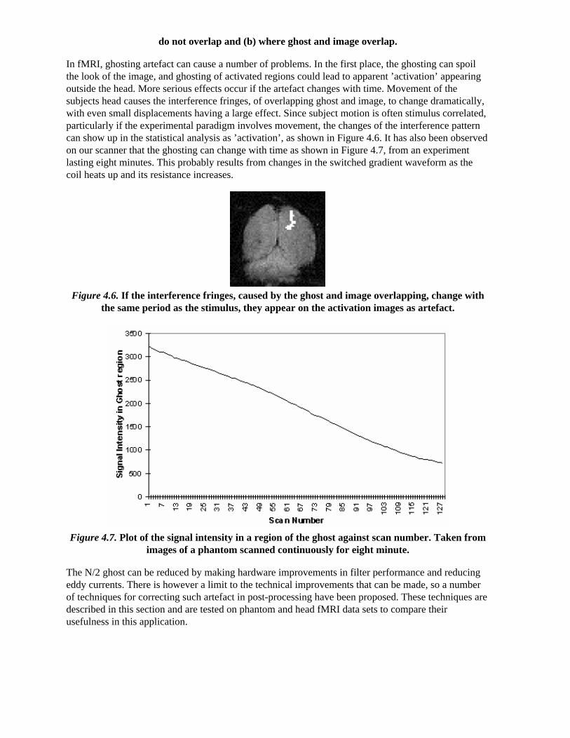
do not overlap and (b) where ghost and image overlap.

In fMRI, ghosting artefact can cause a number of problems. In the first place, the ghosting can spoilthe look of the image, and ghosting of activated regions could lead to apparent ’activation’ appearingoutside the head. More serious effects occur if the artefact changes with time. Movement of thesubjects head causes the interference fringes, of overlapping ghost and image, to change dramatically,with even small displacements having a large effect. Since subject motion is often stimulus correlated,particularly if the experimental paradigm involves movement, the changes of the interference patterncan show up in the statistical analysis as ’activation’, as shown in Figure 4.6. It has also been observedon our scanner that the ghosting can change with time as shown in Figure 4.7, from an experimentlasting eight minutes. This probably results from changes in the switched gradient waveform as thecoil heats up and its resistance increases.

Figure 4.6. If the interference fringes, caused by the ghost and image overlapping, change withthe same period as the stimulus, they appear on the activation images as artefact.

Figure 4.7. Plot of the signal intensity in a region of the ghost against scan number. Taken fromimages of a phantom scanned continuously for eight minute.

The N/2 ghost can be reduced by making hardware improvements in filter performance and reducingeddy currents. There is however a limit to the technical improvements that can be made, so a numberof techniques for correcting such artefact in post-processing have been proposed. These techniques aredescribed in this section and are tested on phantom and head fMRI data sets to compare theirusefulness in this application.

The simplest form of ghost reduction is to apply a phase angle correction to each point in alternatelines of the k-space data. The required phase correction can be determined by eye, and applied to everyimage in the fMRI data set. The effect of eddy currents can be modelled by an alternate echo phasevariation in the read (x-) direction

(4.2)

so by applying a first order correction, ghosting from such effects can be reduced. A mismatch in thesampling can be corrected by a linear shift of the real and imaginary time data.

All these methods go some way towards removing the N/2 ghost, but will not remove ghosts caused bymore complicated phase errors. The subject of N/2 ghosting is extensively covered in a paper byBruder et. al. [5] in which a method based on a calibration scan is proposed. Such a scan is acquiredwith no broadening gradient so, in an ideal case, equivalent points in all the echoes would have thesame phase. Bruder’s method applies a phase correction to force each echo in the calibration scan tohave the same phase, and then applies this same phase correction to the (broadened) image. So if the ith line of the calibration scan has phase qi(x) then the corresponding line in the image is phasecorrected by an angle -qi(x) . This can be carried out practically on a time-point by time-point basis,without directly calculating the phase angles, using the formula

(4.3)

where r and i represent the real and imaginary components of the data point and the subscript crepresents the calibration scan data.

An alternative form of calibration scan has been proposed by Hu [6]. In this case the reference scanconsists of an image acquired under reversed switching gradients. That is to say, if the first line of thenormal image is acquired under a positive read gradient, then the first line of the reference image isacquired under a negative read gradient. These two images could be spliced together, so that the finalimage is made up from only lines that were acquired under a positive read gradient, much in the waythat EPI was first proposed [7]. However Hu proposed that the even lines of the reference scan be usedto correct the odd lines of the actual image, so that a single reference scan can be used to phase correcta whole set of images. Initially all the lines of the normal images and the reference scan are Fouriertransformed in the read direction. Next the even lines of the reference image are reversed. The phasecorrection q that must be applied to these lines in the corresponding normal image in order for them tohave the same phase as the reference image is given by

(4.4)

where the subscript 1 refers to the normal image and the subscript 2 refers to the reference image. Thiscorrection can then be applied to all the images using

(4.5)

again where r is the real component and i is the imaginary component of the complex data point.Finally the images are Fourier transformed along the phase encode direction to form the correctedimage.

This technique can be further extended by collecting two reference scans, without the broadeninggradient applied, one with a positive read gradient for the first echo and the other with a negativegradient. This has the advantage that there is more signal present in the earlier and later lines ofk-space to enable a better calculation of the phase correction required in these lines.

An alternative method that requires no reference scans has been proposed by Buonocore [8]. If twoimages are constructed, one from only the odd echoes, with the even echoes zero filled prior to Fouriertransformation, and one from only the even echoes, with the odd echoes zero filled, then both imageswill display ghosting, one with a positive ghost, and one with a negative ghost (see Figure 4.8). If therewere no phase errors in the odd and even echoes then the phase difference in the object only region(that is where there is no ghost) between these two images would be zero. However if there are phaseerrors, then a phase difference between equivalent points in the odd and even image of 2q(x,y) can bedetected. If the ghost and image do not overlap, it is possible to add the two images together, havingapplied an appropriate phase correction to one, to form a ghost free image. However if they do overlapthen the phase differences are calculated as a function of x only (that is along the read direction) andaveraged through all the lines in the object only region as defined by the user. Having determined thephase difference, the original time data can be corrected by Fourier transformation in the readdirection, multiplying the odd lines by exp(iq(x)) and the even lines by exp(-iq(x)).

Figure 4.8. For an image with no ghosting, splitting k-space into even echoes only, or odd echoesonly, causes ghosting to appear upon Fourier transformation. The image resulting from the even

lines has a positive ghost, whilst the image resulting from the odd lines has a negative ghost.Summing these two image together forms a correct image.

The above five methods were tested on both phantom and head data, with objects that fill and half-fillthe field of view. Examples of their ability to correct the ghosting are shown in Figure 4.9a-b. Most ofthe corrections reduce the ghosting partially in the phantom images. Where the ghost and objectoverlap, the Hu correction with broadening is slightly better at reducing the ring the edge of the ghost.

To quantify the level of ghosting, regions of interest (ROI) were drawn around the object and the ghostregion of the images in which the object half-filled the field of view. Six images of the same phantom,each with different levels of ghosting, were corrected using all five techniques. The mean intensity ofthe ghost as a percentage of the mean intensity of the object for each technique is shown in Figure4.9c. The Hu correction without broadening, does not perform as well as might be expected. This isbecause of the complete failure of the technique in correcting the column in which the external r.f.interference appears, thus producing bright streaks in the ghost region. The Buonocore method appearsin both cases to be the best method.

Figure 4.9a. Examples of the five ghost correction techniques described in the text, applied to128 x 128 and 128 x 64 matrix size phantom images.

Figure 4.9b. Examples of the five ghost correction techniques described in the text, applied to128 x 128 and 128 x 64 matrix size coronal head images.

Figure 4.9c. Ratio of image intensity within the ghost to within the object for the five correctionmethods explained in the text, based on six images (128 x 128 matrix size) each with slightly

different ghosting.

All the above techniques, apart form the Buonocore method, will not correct phase errors that changewith time. Since changes in the ghost do occur with time, adaptations of the above techniques areneeded if they are to deal with such situations. If ghost only and object only regions can be defined, asis the case if the object does not fill the field of view, then a zeroth or first order alternate line phasecorrection can be applied which minimises the signal in the ghost region relative to the object region.This technique can work very well in some cases, however if there is any overlap of image and ghost,then the minimisation can occasionally produce obviously incorrect results. Alternatively, the ghostcan be minimised by eye on the first image in the set, and then the zeroth and first order phasecorrections used to minimise the sum of the square difference between subsequent images and the first.This technique again can generate ridiculous solutions, particularly since this correction has to becarried out before motion correction has been applied. If the assumption is made that the phase errors

change linearly with time then a calibration scan can be obtained before and after the fMRIexperiment, phase correction calculated, and a linear interpolation of the two angles used to correctintermediate images.

These methods were applied to a test fMRI data set of 64 volume images of a phantom and of a head,acquired over a time of 8 minutes. The first order phase correction method used was one where thesignal intensity in the ghost region was minimised by applying the correction shown in equation 4.2.The Bruder correction and the two forms of the Hu correction were applied, such that one correctionmap was calculated, based on the first image in the set, and the same map applied to all images.Reference scans were also acquired at the end of the experiment in order to produce a correction mapfor every image, that was a linear interpolation between that for the first and that for the last. Thegraphs shown in Figure 4.10 show how well each technique corrected the ghost. The striking feature ofthese plots is that many of the methods, in particular the Hu correction without broadening, made theghosting worse. This occurs in the columns in the image where the external r.f. interference is at itsworse. The effect that this has on the image is shown in Figure 4.11a. Again the Buonocore methodworks the best in this situation for both head and ghost data. However, this technique does not alwayswork, as is shown in Figure 4.11b. Since this correction is only based on those lines in which the ghostand image do not overlap, the method has failed where the signal intensity in the central rows is low.An appropriate choice of threshold can prevent low signal intensity having an adverse affect on imagequality, but this highlights the care that must be used in applying any technique.

Figure 4.10. Ratio of image intensity within the ghost to within the object for the five correctionmethods explained in the text, based on six images (128 x 128 matrix size) each with slightly

different ghosting.

(a) (b) Figure 4.11. Examples of the failure of two correction methods to remove the N/2 ghosting. (a)

Hu correction without broadening, (b) Buonocore correction.

Reducing the ghost artefact is not always easy. A technique that works well on one set of data failscompletely on another, and because of this it is useful to be aware of all the possible corrections thatcould be applied. Since it does not require a reference scan, the Buonocore method would appear to bethe most appropriate first choice, however more results obtained from using the method in practicewill be necessary to confirm this.

4.3.2 Removal of External RF Interference

As described in section 2.5.3, external r.f. radiation can cause bright dots of artefact to appear in theimage. Provided that this interference is at a single discrete frequency, and the sampling is linear, onlyone or two pixels in the image will be affected and the image can be cleaned up by replacing thesepixels by the average of their neighbours. Non-linear sampling however means that the singlefrequency interference is spread over a wide range of frequencies after Fourier transformation, andconsequently appears as a line in the image. Not only does such interference spoil the appearance ofthe images, fluctuations in its intensity can cause problems with the analysis of the data. In order tocosmetically remove the interference in such a case, it is easier to re-grid the data, such that it appearsthat it was linearly sampled, and then to remove the few pixels which now contain the interference.The process is illustrated in Figure 4.12.

Figure 4.12. Schematic diagram of process for the removal of r.f. interference bands. (a) Normalimage reconstruction using a 2D Fourier transform. (b) The time data is re-gridded to a largermatrix size and Fourier transformed. The interference now appears as a few discrete points on

the image and can be removed.

The most effective re-gridding of the time data occurs if each line in the image is expanded to fill amuch larger grid, and then the gaps filled in by linear interpolation. The positions in the new grid oflength n, of the existing N data points are found by summing under the sinusoidal gradient waveform,and finding the set of points X1...Xk ...XN , such that

.

(4.6)

The values of the intermediate points are obtained by linear interpolation, so that the intensity at thelocation X in the new grid is given by

.

(4.7)

Re-gridding back from the linear to the sinusoidal grid simply involves extracting the values at thepoints X1...Xk ...XN .

The exact pixels to remove are not easy to determine blindly. It is often the case that they are thebrightest pixels, but not always, and because of this software was written so that the user could easilyselect the pixels that should be removed by looking at the re-gridded image. The application waswritten in the perl scripting language [9], with all the data manipulations and calculations carried outin C programs. The user selects the pixels to remove from the expanded image using the mouse.

Examples of data sets before and after cleaning up are shown in Figure 4.13.

(a) (b) Figure 4.13. Example of the removal of external r.f. interference using the regridding method.

(a) Before removal. (b) After removal.

4.4 Fast IR Sequence for Anatomical Reference Scans

The localisation of the activation response from an fMRI experiment depends on obtaining referencescans which highlight the anatomy of the subjects brain. For this purpose an inversion recovery imagecan be particularly beneficial, since the contrast in the grey and white matter regions of the brain canbe altered by the use of a magnetisation inversion r.f. pulse and an appropriate delay before imaging(see section 2.4.1).

The pulse sequence diagram for a standard inversion recovery experiment is shown in Figure 4.14. At3.0 Tesla the values of the inversion time, TI, required are 400 ms and 1200 ms for white matter null,and grey matter null respectively.

Figure 4.14. Inversion recovery pulse sequence diagram.

Acquiring the reference set, with a suitable number of repeats to gain sufficient signal to noise, cantake several minutes. Much of this time is taken up by the inversion time delay. The fast inversionrecovery sequence uses this time to invert other slices, before going back to image them, as shown inFigure 4.15.

Figure 4.15. Fast inversion recovery pulse sequence diagram.

A constant repetition rate is chosen which is an integer multiple of the required inversion time. Forexample, to obtain grey matter null images with an inversion time of 1200 ms, four slices are invertedat a repetition rate of 300 ms. A comparison of images obtained using the conventional IR sequencewith those obtained using the fast IR sequence shows no difference between the two, however for atypical set of white and grey matter images the fast sequence takes just over 5 minutes compared to 12minutes for the standard IR method. The main limit to the speed of the fast IR acquisition is the rate ofinversion pulses that it is safe to use, because of SAR considerations.

This reduction in time that the subject stays in the scanner helps to keep the subject motivated, andminimises discomfort, which in turn will reduce motion artefact.

4.5 Standard fMRI Protocol

If the results from fMRI experiments are to be reliable, comparable and efficiently obtained, it isnecessary to standardise the way that such experiments are carried out. To this end, a standard fMRIprotocol was written. The aim of this was to provide an experimental outline that contained the basicprocedures that should be carried out, but could be adapted to fit the study in question. The standardfMRI protocol is given in Appendix A.

Correct configuration of the scanner is given purely as a reference, as it is assumed that the operatorwill be familiar with the operation of the 3.0 Tesla scanner [10]. The standard cylindrical phantomused on the 3.0 T scanner contains structure that can enable its orientation to be determined from theimages. A standard orientation of the phantom is given to avoid confusion when looking at the imagesat a later date, and for this reason a phantom reference set of images is always stored with the datafrom that particular experiment. The stability of the scanner is tested each day that fMRI is carried out,by imaging a single slice of a phantom for about 5 minutes. A repetition rate of 10 seconds ensuresthat the effect of stimulated echoes does not interfere with the result. The stability can be calculated ona pixel by pixel basis by dividing the standard deviation of the pixel time course by its mean. Thestability is regarded as satisfactory if this ratio is less than 0.5% throughout the phantom.

Anatomical reference scans are acquired with each data set, so that the precise location of theactivation can be determined. If thick slices (> 1 cm) of the brain are to be imaged in the fMRIexperiment, then it is better to acquire thinner slices for the reference scans, since the reduction inthrough slice susceptibility dephasing that this brings will improve the image quality considerably. Amethod for acquiring these thin slices such that they directly correspond to the thick slices is describedin the protocol.

No details of how the stimulus paradigm should be designed are included in the standard protocol.This is because each paradigm may need to be developed depending on many factors such as the sizeof signal change observed on activation, how the stimulus is presented, how the subject is to respond,and the length of time a subject is able to stay in the scanner. For an initial experiment, a 16 cycleparadigm, with each cycle consisting of 16 seconds of rest and 16 seconds of activity has been shownto be reliable in a number of situations. The results presented later in this thesis, however, show thatfunctional imaging of a single cognitive event is possible, and paradigms that exploit this may yieldextra results over those obtained in an epoch based paradigm.

4.6 References

[1] Van Gelderen, P., Duyn, J. H., Liu, G. and Moonen, C. T. W. (1994) Optimal T2* weighting for

BOLD-type Functional MRI of the Human Brain. Proc. Indian Acad. Sci. (Chem. Sci.) 106,1617-1624.

[2] Singh, M., Patel, P. and Khosla, D. (1996) Estimation of T2* in Functional Spectroscopy during

Visual Stimulation. IEEE Trans. Nucl. Sci. 43,2037-2043.

[3] Menon, R. S., Ogawa, S., Tank, D. W. and Ugurbil, K. (1993) 4 Tesla Gradient Recalled EchoCharacteristics of Photic Stimulation-Induced Signal Changes in the Human Primary Visual Cortex. Magn. Reson. Med. 30,380-386.

[4] Born, P., Rostrup, E. and Larsson, H. B. W. (1997) Dynamic R2* Mapping in Functional MRI. in

Book of Abstracts, 5th Annual Meeting, International Society of Magnetic Resonance in Medicine p.1633.

[5] Bruder H., Fischer, H., Reinfelder, H.-E. and Schmitt, F. (1992) Image Reconstruction for EchoPlanar Imaging with Nonequidistant k-Space Sampling. Magn. Reson. Med. 23,311-323.

[6] Hu, X., and Le, T. H. (1996) Artefact Reduction in EPI with Phase-encoded Reference Scan Magn.Reson. Med. 36,166-171.

[7] Mansfield, P. (1977) Multi-Planar Image Formation Using NMR Spin Echoes. J. Phys. C. 10,L55-L58.

[8] Buonocore, M. H. and Gao, L. (1997) Ghost Artefact Reduction for Echo Planar Imaging UsingImage Phase Correction. Magn. Reson. Med. 38,89-100.

[9] See Wall, L. and Schwartz, R. Programming Perl, OReilly & Associates.

[10] Mansfield, P., Coxon, R. and Glover, P. (1994) Echo-Planar Imaging of the Brain at 3.0 T: FirstNormal Volunteer Results. J. Comput. Assist. Tomogr. 18,339-343.

Chapter 5 - Functional MRI using Interleaved EPI

5.1 Introduction

One of the largest problems in using echo planar imaging is the level of image distortion due tosusceptibility, that is observed. This can make some structures in the brain, such as the basal ganglia,hard to detect using EPI especially at 3 Tesla. As was mentioned in Chapter 2, the Fourier imagingtechniques (2DFT) suffer much less from susceptibility distortion than EPI does, and this is one reasonwhy these techniques are used in routine clinical scans. It is not impossible to carry out fMRI using2DFT methods, particularly the fast techniques such as FLASH [1], but EPI will always have thespeed advantage over such techniques. This is because the entire image is acquired from a single freeinduction decay (FID), whereas FLASH only acquires one line from each FID.

In order to improve the quality images in fMRI experiments, an approach that can be taken is to use atechnique which is a hybrid of EPI and 2DFT, called interleaved EPI. This technique acquires theimage in two or more FIDs, thereby trading some of the speed of EPI to gain some of the imagequality of 2DFT.

Interleaved EPI was first proposed by McKinnon [2], as a way of implementing EPI on a standardclinical scanner, which did not have the necessary fast ramping gradients. Later it was alsodemonstrated that the technique could be used for fMRI [3]. Interleaved EPI also has benefits howeverfor scanners which can carry out conventional EPI, ranging from reducing distortion, improvinglinewidth, to increasing signal to noise.

This chapter describes the theory and implementation of interleaved EPI at 3 Tesla, for use in fMRIexperiments. It outlines some of the benefits of using interleaved EPI, and the problems that occur inits use for fMRI.

5.2 The Theory of Interleaved EPI

5.2.1 K-Space Coverage and Gradient Waveforms

Interleaved EPI acquires all the data points required to make up the image in several FIDs. The easiestway to picture how this is done is to look at the k-space coverage diagram (Figure 5.1) for a two shotinterleaved EPI sequence. The first interleave covers the whole of k-space in alternate lines, and thenthe second pass fills in the lines between. The same principle holds for any number of interleaves, upuntil the technique essentially becomes a 2DFT experiment.

Figure 5.1. K-space coverage diagram for a two shot interleaved EPI sequence.

The technique is sometimes referred to as segmented EPI, since k-space is covered in two or moresegments. There are other ways that k-space can be segmented, for example, acquiring the positive ky

values in the first shot, and negative values in the second. It seems appropriate to refer to the kind oftechnique shown in Figure 5.1 as interleaved EPI, since the two shots are indeed interleaved onreconstruction, and to refer to other multi-shot techniques as segmented EPI.

The pulse sequence diagram required for two shot interleaved EPI is shown in Figure 5.2. Both shotsare essentially MBEST modules, but with three differences between the first and second shot. Firstlythere is a difference in the length of the pre excursion of the blipped gradient. This ensures that thephase encoding is slightly different for each shot, so that every line of k-space is acquired. Assumingthat the magnitude of the blipped pre-excursion gradient is the same as the blipped gradient itself, thenthe excursion must increase in length by half of the duration of one blip, for each interleave. Sinceincreasing the length of the pre-excursion delays, albeit slightly, the time of the echo, an appropriatedelay must be added in the earlier interleave to compensate.

Figure 5.2. Pulse sequence diagram for a two shot interleaved EPI experiment.

The other two differences relate to discontinuities in the phase and magnitude of the signal along the ky direction in the final image.

5.2.2 Correcting for Discontinuities in K-Space

The second difference between shots in the pulse sequence diagram relates to the magnitude of thetransverse magnetisation vector after the r.f. pulse. If the magnitude of the longitudinal magnetisationprior to the experiment is M0, then following a 90 degree pulse the transverse magnetisation will be

M 0, and the longitudinal magnetisation will be zero. In the duration, TR, between the first and second

r.f. pulses the longitudinal magnetisation will recover through T1 relaxation, and following a second

90 degree pulse the transverse magnetisation will be

.

(5.1)

Unless TR >> T1, the signal intensity of the two interleaves will therefore be significantly different.

This leads to discontinuities in k-space and causes ghosting artefact, as demonstrated in Figure 5.3.The effect can be compensated for by reducing the flip angle of the first pulse.

(a) (b) Figure 5.3. Differences in the amplitude or phase between the two interleaves that make up the

image, causes ghosting.

Figure 5.4. (a) Discontinuities along the central line of k-space lead to ghosting artefact. (b) Byshifting the echo time of successive interleaves, these discontinuities are smoothed out.

The z-magnetisation prior to the nth interleave is given by

(5.2)

and for constant signal following each excitation

.

(5.3)

These equations can be solved iteratively, with the last flip angle being 90 degree, to find the flipangles for each of the interleaves. These equations only hold for one value of T1, and so

discontinuities between interleaves in the signal from tissue with a different value of T1 will still

occur. To reduce this problem McKinnon suggests calculating a slightly longer series than necessary,and only using the first part of the series [4].

In using interleaved EPI for fMRI, many images are obtained with a constant repetition rate. Thismeans that a constant flip angle can be used, and after the first few images have been acquired themagnitude of the longitudinal magnetisation reaches a steady state.

The third difference in the pulse sequences between interleaves, acts to reduce phase discontinuities inthe time data. Off-resonance phase errors, due to field inhomogeneity, susceptibility and chemicalshift, evolve constantly with time. Since in each interleave alternate lines are acquired under oppositeread gradients, these lines must be reversed in the time data matrix prior to Fourier transformation.This leads to steps in the phase, which may cause ghosting artefact. This can be a problem inconventional EPI, but the problem is compounded in N shot interleaved EPI, since the first N lines areall acquired at the same time in the echo train, and thus the steps are N times longer (see Figure 5.4a).

To compensate for this, at least along the central line of k-space, a slight time delay of magnitude

(5.4)

is added to the nth interleave (Tx is the time needed to acquire one line in k-space). This has the effect

of smoothing out the discontinuities (see Figure 5.4b) [5,6].

5.2.3 Multi-Slice Interleaved EPI

Since it is commonly required to image several slices when carrying out an fMRI experiment, thesignal to noise ratio can be improved by employing a multi-slice technique. The k-space diagram formulti-slice interleaved EPI is shown in Figure 5.5.

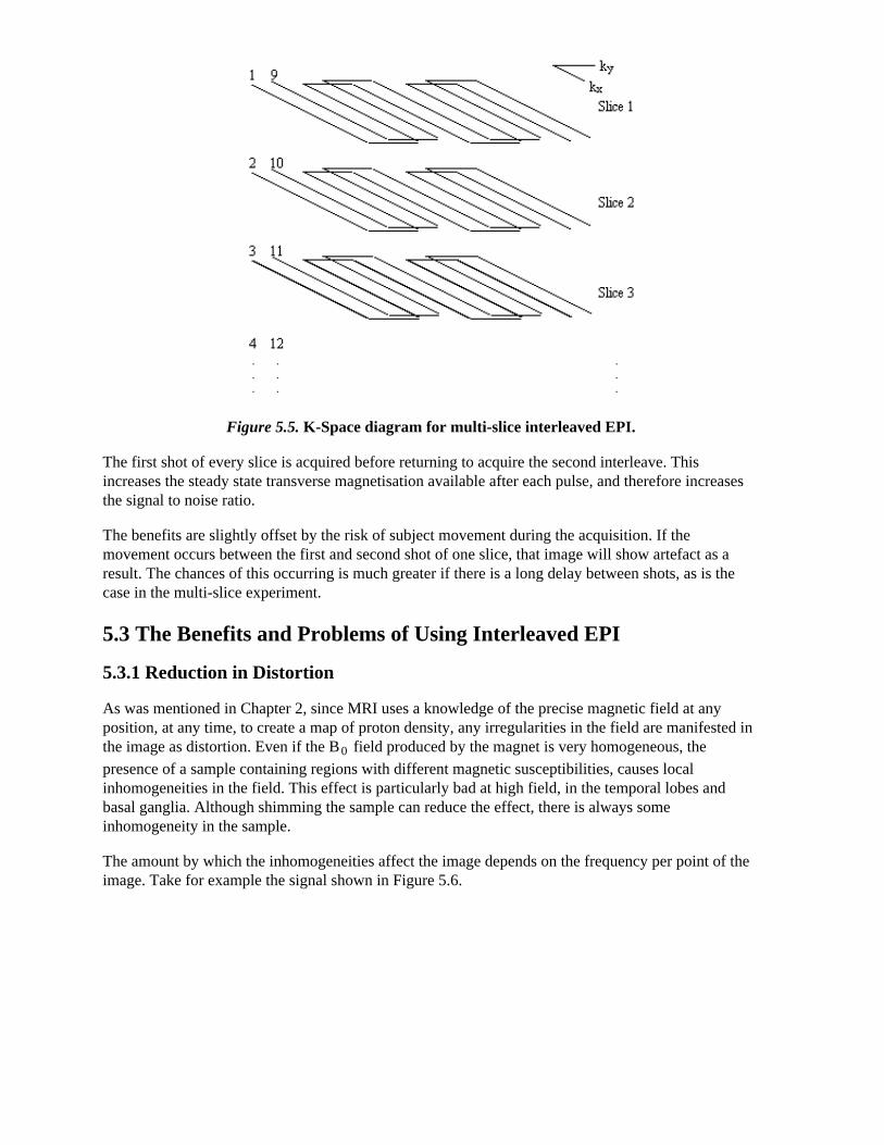
Figure 5.5. K-Space diagram for multi-slice interleaved EPI.

The first shot of every slice is acquired before returning to acquire the second interleave. Thisincreases the steady state transverse magnetisation available after each pulse, and therefore increasesthe signal to noise ratio.

The benefits are slightly offset by the risk of subject movement during the acquisition. If themovement occurs between the first and second shot of one slice, that image will show artefact as aresult. The chances of this occurring is much greater if there is a long delay between shots, as is thecase in the multi-slice experiment.

5.3 The Benefits and Problems of Using Interleaved EPI

5.3.1 Reduction in Distortion

As was mentioned in Chapter 2, since MRI uses a knowledge of the precise magnetic field at anyposition, at any time, to create a map of proton density, any irregularities in the field are manifested inthe image as distortion. Even if the B0 field produced by the magnet is very homogeneous, the

presence of a sample containing regions with different magnetic susceptibilities, causes localinhomogeneities in the field. This effect is particularly bad at high field, in the temporal lobes andbasal ganglia. Although shimming the sample can reduce the effect, there is always someinhomogeneity in the sample.

The amount by which the inhomogeneities affect the image depends on the frequency per point of theimage. Take for example the signal shown in Figure 5.6.

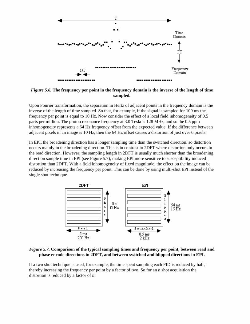
Figure 5.6. The frequency per point in the frequency domain is the inverse of the length of time sampled.

Upon Fourier transformation, the separation in Hertz of adjacent points in the frequency domain is theinverse of the length of time sampled. So that, for example, if the signal is sampled for 100 ms thefrequency per point is equal to 10 Hz. Now consider the effect of a local field inhomogeneity of 0.5parts per million. The proton resonance frequency at 3.0 Tesla is 128 MHz, and so the 0.5 ppminhomogeneity represents a 64 Hz frequency offset from the expected value. If the difference betweenadjacent pixels in an image is 10 Hz, then the 64 Hz offset causes a distortion of just over 6 pixels.

In EPI, the broadening direction has a longer sampling time than the switched direction, so distortionoccurs mainly in the broadening direction. This is in contrast to 2DFT where distortion only occurs inthe read direction. However, the sampling length in 2DFT is usually much shorter than the broadeningdirection sample time in EPI (see Figure 5.7), making EPI more sensitive to susceptibility induceddistortion than 2DFT. With a field inhomogeneity of fixed magnitude, the effect on the image can bereduced by increasing the frequency per point. This can be done by using multi-shot EPI instead of thesingle shot technique.

Figure 5.7. Comparison of the typical sampling times and frequency per point, between read andphase encode directions in 2DFT, and between switched and blipped directions in EPI.

If a two shot technique is used, for example, the time spent sampling each FID is reduced by half,thereby increasing the frequency per point by a factor of two. So for an n shot acquisition thedistortion is reduced by a factor of n.

An example of the reduction in image distortion is shown in Figure 5.8. These three transaxial slicesthrough the brain have matrix size 128 x 128, and were acquired using single shot (conventional) EPI,two shot and four shot interleaved EPI. They were acquired with a read gradient switching rate of 615Hz, meaning that the sampling times for the single, two and four shot images were 104 ms, 52 ms and26 ms respectively. The reduction in distortion in going from single shot to four shot is very apparent,however it can be noted that there is a greater level of ghosting artefact on the four shot image than onthe single shot one.

(a) (b) (c) Figure 5.8 A transaxial slice through the brain acquired using (a) single shot, (b) two shot and (c)

four shot interleaved EPI. The level of distortion is greatly reduced in the four shot case,compared to the single shot.

This is the most significant benefit of using interleaved EPI, that by increasing the number ofinterleaves, the level of the distortion in the image due to field inhomogeneity reduces.

5.3.2 Improvement in Linewidth

A second benefit of interleaved EPI is in the reduction in linewidth, which results again from theincrease in frequency per point in the image.

As was described in Chapter 2, spin-spin relaxation and the effect of field inhomogeneity causes thetransverse magnetisation to decay, with a time constant T2

* . This has the effect of convolving the

image with a point spread function, as shown in Figure 5.9.

Figure 5.9The effect of T2* decay on the sharpness of a line through an image. The smaller the

value of T2* , the wider the point spread function, and the more smoothed the profile becomes.

The point spread function is the Fourier Transform of the T2* decay

,

(5.5)

and has the form

.

(5.6)

If two points of equal magnitude in the image are separated by Dw, then the total signal as a functionof w is of the form

.

(5.7)

The Rayleigh criterion [7] states that two pixels are resolved when two pixels of intensity S0 , are

separated by one of intensity less than 0.81S0 , as shown in Figure 5.10.

Figure 5.10. The Rayleigh criterion applied to the resolution of two pixels subject to T2 * linebroadening. The intensity of the central pixel must be less than 0.81 that of the intensity of the

two pixels it separates.

So using the condition

(5.8)

the minimum frequency per point separation required to obtain true pixel resolution is given by

.

(5.9)

Thus for a typical value of T2 * at 3 T of 60 ms, the required frequency per point is 16 Hz. If high

resolution imaging is being carried out then it is quite possible that the pixel resolution is not the trueresolution. For example, acquiring a 2562 matrix with a switched gradient frequency of 500 Hz usingconventional EPI will give a frequency per point of just under 4 Hz. This is below the 16 Hz frequencyper point required for true pixel resolution. However by using a two shot interleaved EPI technique thefrequency per point will increase to 8 Hz, and a four shot technique will double this value again toabout 16 Hz.

Figure 5.11 shows three images of a cylindrical phantom containing a 3 mm diameter glass rod,surrounded by water doped to have a T2

* similar to the brain. The phantom is imaged to a pixel

resolution of 1 mm, with single shot, two shot and four shot EPI, and line profiles through the rod, asindicated by the black line on the images, are shown. The line profile shows a clear increase indefinition of the glass rod in the four shot case, compared to the single shot case, indicating theimprovement in real resolution obtained in this case by using interleaved EPI.

Figure 5.11 Line profile through a phantom imaged using (a) single shot, (b) two shot and (c)four shot interleaved EPI. The pixel resolution is 1 x 1 mm2 and the glass rod in the phantom

has diameter 3 mm. The narrower point spread function, in the broadening direction, of the fourshot image means that the rod is better defined than in the single shot case.

5.3.3 The Benefits of using Interleaved EPI for fMRI

There are several approaches that can be taken in using interleaved EPI to improve the results of anfMRI experiment.

If for example the fMRI image is of poor quality, due to susceptibility distortions, the distortion can bereduced by using interleaved EPI whilst maintaining the same resolution. The distortion in this casewill be reduced by the number of interleaves used.

Alternatively, if the level of distortion is acceptable, the resolution can be increased by reducing theswitched gradient frequency by half and doubling the number of interleaves. The frequency per pointin this case will stay the same, and so therefore will the distortion. Interleaved EPI offers real benefitsin carrying out high resolution fMRI at high field.

Without increasing the resolution or the distortion, the benefits of interleaved EPI can be seen in anincreased signal to noise ratio, and reduced gradient current requirements. This can be achieved bylowering the switched gradient frequency, thereby increasing the time taken to sample one line ink-space. This reduces the sampling bandwidth required and increases the signal to noise ratio by thesquare root of the number of interleaves used. By reducing the current requirement, the level ofgradient heating is also reduced.

For larger matrix sizes and lower gradient switching rates, the linewidth broadening may become alimitation. In this situation, interleaved EPI can be used to regain true resolution.

The combination of gradient switching rate, and matrix size, with the number of interleaves, can bringbenefits in resolution, distortion, gradient heating, and signal to noise, although the increased numberof acquisitions means that the experimental duration may be longer.

Recently a number of groups have demonstrated the use of interleaved EPI for high resolution fMRI ofthe visual cortex at high field [8],9] and also the development of the technique to carry out interleavedecho volumar imaging (EVI) [10].

5.3.4 Ghosting Artefact in Interleaved EPI

As already mentioned above, any differences in phase or intensity between interleaves will show up inthe images as ghosting artefact. These differences can be due to subject movement or instability in thescanner hardware. In addition, the ghosting caused by the reversal of lines acquired under the negativeread gradient (Nyquist or N/2 ghost) is made worse since the positive and negative gradient pulses aregrouped in blocks by the interleaving. Such artefacts, which change with time make fMRI difficult toperform, particularly at high resolution where signal to noise is low and small movements mean alarge pixel displacement. The magnitude of the changes in the image due to artefact are often greaterthan the contrast changes due to the BOLD effect.

The first line of attack on such problems is to attempt to remove them at source. Motion can bereduced by restraining the subject’s head, and by careful planning of the stimulus paradigm.Unfortunately high resolution fMRI using interleaved EPI requires long experiments, due to its lowsignal to noise. This makes the subject more uncomfortable and prone to move. To reduce the N/2ghosting problem an asymmetric EPI experiment could be used [11]. This only acquires the data underone polarity of read gradient and so is not quite as efficient as conventional interleaved EPI.

Instability from shot to shot in the hardware can be measured using a navigator echo [12,13]. In itssimplest form, a navigator echo is a sample of the FID, prior to the application of the imaginggradients. The phase of this sample can be calculated for each of the interleaves in the image, and thena bulk phase correction applied to normalise the data. This technique was included in the interleavedEPI pulse sequence, acquiring a number of sample points prior to the imaging gradients. The meanphase of these data points was calculated and a phase correction determined to normalise these valuesfor each interleave. These factors were applied to the actual image data prior to Fourier transformation.

Other forms of navigator echoes have been proposed for the correction of interleaved EPI data [14]. Inparticular, the obvious extension of applying a gradient in one direction during the navigator echoacquisition, so as to make the echo sensitive to uni-directional movement, has been suggested.

Even after applying the navigator correction there is still a significant amount of ghost present, mostprobably due to subject movement. To reduce this, it is necessary to apply some form of correction tothe data in post-processing. The most straightforward correction is a zeroth order phase shift, wherethe same phase change is applied to every point in the interleave. In order to successfully use such acorrection as a post-processing technique on fMRI data, it is necessary to decide upon some measureof the amount of ghosting.

The Fourier transform (FT) of the central column of k-space, represents the D.C. component of eachline in the image. The amount of ghost can be determined by selecting this column, applying the phasecorrection and FT, and measuring the ratio of the central points to the edge points, as shown in Figure5.12. This method works well for a two shot technique, where the ghost appears at the edges, but isless successful if more interleaves are used and the ghost appears throughout the image.

Figure 5.12 Profile of Fourier Transform of the central line of k-space for two shot interleavedEPI images, (a) with severe ghosting and (b) with little ghosting. The ratio of the central lines of

this profile to the outside lines is a maximum for a ghost free image.

Since the origin of the artefact is motion, it seems appropriate to apply some form of motioncorrection. To do this it is necessary to have some measure of how well any processing corrects thedata. One possibility is to define the regions where any ghosting would be expected to be manifestedand try to reduce the signal intensity in this area [15]. If this is not possible then some other measure ofthe level of ghosting is required. Atkinson and Hill [16] have suggested that an entropy term of theform

(5.10)

where Si is the intensity of the ith pixel in the image, would be one such measure. They propose

motion correcting the interleaves until the term in equation 5.10 is a minimum.

Until a suitable solution for the problem of the ghosting is found, high resolution interleaved EPI willbe difficult to use in practice.

5.4 Implementation at 3.0 Tesla

To demonstrate the viability of using interleaved EPI to carry out fMRI at 3.0 Tesla, three experimentswere performed.

5.4.1 High Resolution fMRI

A two shot multislice interleaved EPI technique was used to acquire a 256 x 256 matrix size image,using a switching rate of 1.04 kHz. Eight slices of thickness 4.5 mm, covering the visual cortex wereacquired in eight seconds, during periods of visual stimulation from the pattern reversal (4 Hz) of acheckerboard pattern. There were 32 seconds of stimulation followed by 32 seconds of rest, repeated16 times. The in-plane resolution was 0.75 x 0.91 mm2. A zeroth order phase correction was appliedto one interleave, until the Fourier transform of the central line of k-space had the maximum ratio ofsignal in the inner points to signal in the outer points. The images were re-registered, but no spatial ortemporal smoothing applied. The fMRI data was correlated to a square wave of the same period andphase as the stimulus and p-values calculated on the basis on peak height and spatial extent of thecorrelation maps using the theory of Gaussian random fields (see Chapter 6).

The resulting activation map is shown in Figure 5.13. The coloured regions represent the regions thatcorrelate well to the stimulus (p>0.05). The background images are the average of the actual fMRIdata set, so that the resolution seen in these images is the same as that of the activation maps. Regionsof activation can be seen in the primary visual cortex and visual association areas. The change in theprimary visual cortex upon activation was approximately 20%.

Figure 5.13 High resolution two shot interleaved EPI functional images for a visual stimulus inthe right visual field. Activation (p>0.005) is overlaid on the average of the images used for the

fMRI analysis.

5.4.2 Low distortion fMRI

Low distortion EPI images were acquired using a two shot multislice interleaved EPI technique with amatrix size of 128 x 128 and a switching rate of 1.9 kHz. These were compared with images from asingle shot experiment with the same matrix size. The activation paradigm consisted of 32 seconds ofthe subject observing the pattern reversal (4 Hz) of a checkerboard display whilst finger tapping,followed by 32 seconds of rest, repeated eight times. The whole brain, in each experiment, wasscanned in 16 slices, in a period of 8 seconds. The images were registered and spatially smoothed(FWHM 4 mm), and correlated to a square wave of the same period and phase as the stimulus.Activation maps were thresholded, using the theory of Gaussian random fields, based on peak heightand spatial extent. The activation maps were overlaid on white matter inversion recovery images (TI1200 ms) acquired using either the single shot or two shot technique.

The resulting images are shown in Figure 5.14. Both methods produced very similar activation maps,with slightly more activation detected in the single shot technique. This is because the shot-to-shotsignal to noise was not quite as good in the two shot experiment, presumably due to slight subjectmovement between interleaves. The level of distortion is slightly less in the two shot case and theseresults demonstrate the viability of carrying out low distortion interleaved EPI at 3.0 T.

Figure 5.14 Activation images from two experiments both involving a the same visually cuesmotor task. The top set of images were acquired using single shot EPI, and the bottom set

acquired using two shot interleaved EPI.

5.4.3 High Resolution Anatomical References Images for fMRI.

One final application of interleaved EPI is to produce high resolution anatomical images to overlay theactivation data on, with the level of distortion being the same in each case, allowing directsuperposition.

A single shot EPI, functional imaging experiment was performed using a matrix size of 128 x 64, anda switching rate of 1.04 kHz. The activation paradigm consisted of 16 seconds of viewing a flashingLED display, and pressing a hand held button at the same rate, followed by 16 seconds of rest,repeated 16 times. The visual cortex was scanned in eight slices, every 2 seconds (resolution 3 x 3 x 9 mm3). Following the activation experiment, the switched and broadening gradient strengths weredoubled and four volume images of the same slices were obtained using a two shot interleaved EPIsequence, having twice the in-plane resolution (1.5 x 1.5 mm2). These were used as backgroundimages for the activation maps to be overlaid upon. The activation maps were interpolated up to twicetheir size, and registered to the high resolution images. The activation images are shown in Figure5.15.

Figure 5.15 Low resolution activation images (3 x 3 mm2 in-plane) for a visual stimuli, overlaidon high resolution (1.5 x 1.5 mm2 in-plane) background T2

* weighted images.

5.5 Summary

The results show that high resolution fMRI has the potential to detect small regions of functionalactivity. If such high resolution images are to be obtained then a multi shot EPI sequence is mostprobably required so that the images do not suffer too greatly from distortion. The main problem withhigh resolution interleaved EPI is the artefact caused by subject movement, and until a robustpost-processing correction technique has been demonstrated, it is going to be difficult to gain usefulresults.

The interleaved EPI sequence however still has other applications on a high gradient performance 3.0Tesla scanner. The reduction in distortion that the multi shot techniques brings, will benefit studies ofthe basal structures of the brain in particular. The ability to obtain high resolution anatomical images,with the same distortion as the original activation images, allows confident anatomical localisation ofthe activation, since the resolution is higher than the single shot images, but there will be less risk ofmis-registration of structures in the functional images to the anatomical images that might be the caseif 2DFT images were used.

5.6 References

[1] Frahm, J., Merboldt, K.-D. and Hänicke, W. (1993) Functional MRI of Human Brain Activation atHigh Spatial Resolution. Magn. Reson. Med. 29,139-144.

[2] McKinnon, G. C., Eichenberger, A. C., von Weymarn, C. A. and von Schulthess, G. K. (1992)Ultra-Fast Imaging Using an Interleaved Gradient Echo Planar Sequence in Book of Abstracts, 11thAnnual Meeting, Society of Magnetic Resonance in Medicine p.106.

[3] Butts, K., Riederer, S. J., Ehman, R. L., Thompson, R. M. and Jack, C. R. (1994) Interleaved EchoPlanar Imaging on a Standard MRI System. Magn. Reson. Med. 31,67-72.

[4] McKinnon, G. C. (1993) Ultrafast Interleaved Gradient-Echo-Planar Imaging on a StandardScanner. Magn. Reson. Med. 30,609-616.

[5] Feinberg, D. A. and Oshio, K. (1994) Phase Errors in Multi-Shot Echo Planar Imaging. Magn.Reson. Med. 32,535-539.

[6] Mugler III, J. P. and Brookeman, J. R. (1996) Off-Resonance Image Artefacts in Interleaved-EPIand GRASE Pulse Sequences. Magn. Reson. Med. 36,306-313.

[7] Lord Rayleigh (1879) Investigations in Optics with special reference to the Spectroscope. Phil. Mag. 8,261-274.

[8] Kim, S.-G., Hu, X., Adriany, G. and Ugurbil., K. (1996) Fast Interleaved Echo-Planar Imagingwith Navigator: High Resolution Anatomic and Functional Images at 4 Tesla. Magn. Reson. Med.35,895-902.

[9] Thulborn, K. R., Voyvodic, J., Chang, S. Y., Song, D., Blankenberg, F., Davis, D. and Zeki, S.(1997) High Spatial Resolution, Echo-Planar fMRI at 3.0 Tesla Resolves Specialized Functions of theHuman Visual Cortex in Book of Abstracts, 5th Annual Meeting, International Society of MagneticResonance in Medicine p.7.

[11] Tan, S. G., Wong, E. C., Li, S.-J., Song, A. W. and Hyde, J. S. (1995) Interleaved Echo VolumarImaging in Book of Abstracts, 3rd Annual Meeting, Society of Magnetic Resonance p.620.

[12] Hennel, F. and Nédélec, J.-F. (1995) Interleaved Asymmetric Echo-Planar Imaging. Magn. Reson. Med. 34,520-524.

[13] Ehman, R. L. and Felmlee, J. P. (1989) Adaptive Technique for High-Definition MR Imaging ofMoving Structures. Radiology 173,255-263.

[14] Hu, X. and Kim, S.-G. (1994) Reduction of Signal Fluctuation in Functional MRI UsingNavigator Echoes. Magn. Reson. Med. 31,495-503.

[15] Kim, S.-G., Hu, X., Adriany, G. and Ugurbil., K. (1996) Fast Interleaved Echo-Planar Imagingwith Navigator: High Resolution Anatomic and Functional Images at 4 Tesla. Magn. Reson. Med.35,895-902.

[16] Robson, M. D., Anderson, A. W. and Gore, J. C. (1997) Diffusion-Weighted Multiple Shot EchoPlanar Imaging of Humans without Navigation. Magn. Reson. Med. 38,82-88.

[17] Atkinson, D. and Hill, D. Private communication.

Chapter 6 - The Analysis of fMRI Data

6.1 Introduction

This chapter deals with the way in which the raw data from an fMRI experiment is analysed. The aimof such analysis is to determine those regions in the image in which the signal changes upon stimuluspresentation. Although it is possible to devise many different techniques for detecting activation, ifthese techniques are to be used in practice it is necessary to know how much confidence can be placedin the results. That is to say, what is the probability that a purely random response could be falselylabeled as activation. This requires an understanding of the statistics behind the technique used.

Many of the statistically robust techniques used to analyse fMRI data have been developed from PET.These try to model the time course that is expected, and determine how well each pixel’s temporalresponse fits this model. However, since fMRI experiments allow a much greater time resolution thanPET, it is possible to carry out experiments which determine the order in which different cognitiveevents occur. Analysis of the data from such an experiment requires a ’non-directed’ technique whichmakes few assumptions about the timings of the activation responses expected.

There are three stages to the analysis of the data from any fMRI experiment (Figure 6.1). Firstly thereare the pre-processing steps, which can be applied to the data to improve the detection of activationevents. These include registering the images, to correct for subject movement during the experiment,and smoothing the data to improve the signal to noise ratio. Next, the statistical analysis, which detectsthe pixels in the image which show a response to the stimulus, is carried out. Finally the activationimages must be displayed, and probability values, which give the statistical confidence that can beplaced in the result, quoted.

Figure 6.1 Steps involved in the processing of fMRI data

In order to analyse the data from the experiments explained in Chapter 7, a suite of programs werewritten, which implement existing and novel analysis techniques for carrying out the steps outlinedabove. These techniques are described in detail in the following sections.

6.2 Preparing MR Images for Statistical Analysis

There are a number of steps that can be carried out prior to the statistical analysis of the data. Each ofthese steps is independent and offers different benefits. There is an analysis time penalty to be paid foreach of the steps, some of which can take times of the order of hours. The theory and implementationof each step is described below, with an integrated package explained in the final section.

6.2.1 Image Formation, Data Reduction and Global Normalisation

The raw time data from the scanner requires Fourier transformation to form the image. The raw data isstored as complex numbers, one for each pixel in the image. Correction for N/2 ghost artefact (seeSection 4.3.1) can be carried out at this stage by changing the phase angle between real and imaginarydata points of alternate lines. The extent of correction required can be determined by eye, adjusting thephase angle until the N/2 ghost in the first image in the set is minimised. The same correction can thenbe applied to every image in the fMRI data set. Alternatively one of the methods suggested in Chapter4 can be utilised. Failure to eliminate any ghost artefact can cause activations from within the head tobe aliased in the ghost.

Two dimensional fast Fourier transformation (FFT) is carried out using a standard routine[1], with theimages being stored as 4 byte signed integers (shorts). The data is also scaled to utilise the whole rangeof the short data type (+/- 32767).

Two data reducing steps are performed, which cut down on the number of calculations that need to becarried out. Experimental pre-scans (saturation scans), which ensure that the effects of T1 recoveryhave reached a steady state, can be removed from the beginning of the data set. Also the matrix sizecan be reduced so that it covers only the brain.

Changes in the global blood flow to the brain (gCBF), as well as instability in the scanner hardware,can cause the mean intensity of the images to vary with time, regardless of functional activity. A plotof the mean intensity of an image of a single slice, acquired every 2 seconds is shown in Figure 6.2.

Figure 6.2 Plot of the fluctuations in global intensity of a single slice throughout an fMRIexperiment lasting 15 minutes.

Such fluctuations mean that the response to each stimulus is not identical, and reduces the power ofany statistical test performed. In order to remove this effect, each image can be scaled so that it has amean equal to some pre-determined value, or to the global mean of the whole data set. Since there arefluctuations in the intensity of the artefact caused by external r.f. interference, which are independentof the variation in the true image intensity, it is necessary to exclude these regions from the calculationof the image mean. Regions to exclude are chosen by the user, prior to the normalisation.

6.2.2 Motion Correction

Subject head movement, during the experiment is a major source of artefact in fMRI data. Changes inpixel intensity at the edges of the brain, upon even slight movement, can be far greater than the BOLDactivation response. It is common therefore in fMRI data analysis to perform some correction whichreduces this effect[2].

The approach taken here is to correct only for in-plane translations and rotations of the head within theimage. Working on a slice-by-slice basis, the first image is taken to be the reference image, to whichall other images of that slice are to be aligned. Two dimensional rotations and translations are appliedto the second image, and the sum of the squares of the difference (ssd) between pixels in the first andsecond image are calculated. Further translations and rotations are applied to the image until the ssd isminimised, using a standard routine. All subsequent images are realigned in the same way.

This technique is quite robust, and does not have difficulty in converging. One obvious extension ofthis would be to go to a three dimensional technique. This would have the advantage of more fullycorrecting the head motion, and would also be a faster technique, but introduces the problem ofinterpolating the data to give isometric voxels. Additional corrections that could be applied includethose which remove cardiac and respiratory effects[3], and those which correct for the history of the spins[4].

6.2.3 Spatial Smoothing

Any reduction in the random noise in the image will improve the ability of a statistical technique todetect true activations[5]. Spatially smoothing each of the images improves the signal-to-noise ratio(SNR), but will reduce the resolution in each image, and so a balance must be found betweenimproving the SNR and maintaining the resolution of the functional image.

The simplest form of smoothing to apply is a 9 point filter, such as the one shown below.

If S(x,y) is the image intensity of a pixel at position (x,y) in the image, then upon applying the abovefilter this pixel will have value

(6.1)

Such a filtering technique is simple and quick, but lacks control of the width of the filter. Analternative is to convolve the image with a three dimensional Gaussian function, of the form

(6.2)

where sx, sy and sz are the standard deviations of the Gaussian in each direction. A good estimate of theextent of such a smoothing is given by the full width at half maximum (FWHM) of the Gaussiankernel. The relationship between standard deviation and FWHM is

FWHM = 2.35s. (6.3)

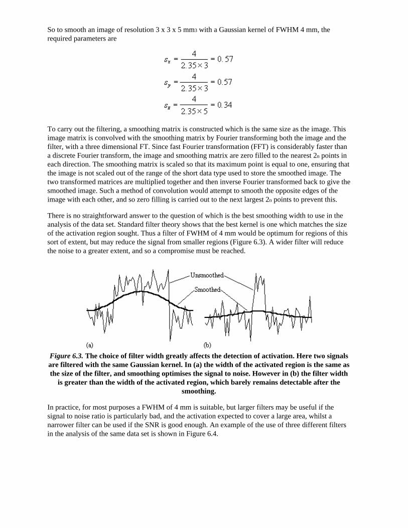
So to smooth an image of resolution 3 x 3 x 5 mm3 with a Gaussian kernel of FWHM 4 mm, therequired parameters are

To carry out the filtering, a smoothing matrix is constructed which is the same size as the image. Thisimage matrix is convolved with the smoothing matrix by Fourier transforming both the image and thefilter, with a three dimensional FT. Since fast Fourier transformation (FFT) is considerably faster thana discrete Fourier transform, the image and smoothing matrix are zero filled to the nearest 2n points ineach direction. The smoothing matrix is scaled so that its maximum point is equal to one, ensuring thatthe image is not scaled out of the range of the short data type used to store the smoothed image. Thetwo transformed matrices are multiplied together and then inverse Fourier transformed back to give thesmoothed image. Such a method of convolution would attempt to smooth the opposite edges of theimage with each other, and so zero filling is carried out to the next largest 2n points to prevent this.

There is no straightforward answer to the question of which is the best smoothing width to use in theanalysis of the data set. Standard filter theory shows that the best kernel is one which matches the sizeof the activation region sought. Thus a filter of FWHM of 4 mm would be optimum for regions of thissort of extent, but may reduce the signal from smaller regions (Figure 6.3). A wider filter will reducethe noise to a greater extent, and so a compromise must be reached.

Figure 6.3. The choice of filter width greatly affects the detection of activation. Here two signalsare filtered with the same Gaussian kernel. In (a) the width of the activated region is the same asthe size of the filter, and smoothing optimises the signal to noise. However in (b) the filter width

is greater than the width of the activated region, which barely remains detectable after the smoothing.

In practice, for most purposes a FWHM of 4 mm is suitable, but larger filters may be useful if thesignal to noise ratio is particularly bad, and the activation expected to cover a large area, whilst anarrower filter can be used if the SNR is good enough. An example of the use of three different filtersin the analysis of the same data set is shown in Figure 6.4.

(a) (b) (c)Figure 6.4. The use of three different smoothing filters on the same fMRI data set of a hand

clenching experiment, of 3 x 3 mm2 in-plane resolution. Areas that correlate well to the task areshaded in white, with the same p-value used for all three activation maps. (a) No filtering

applied. (b) 7 mm FWHM filter applied. (c) 15 mm FWHM filter applied.

6.2.4 Temporal Smoothing

As well as smoothing in the spatial domain, improvements in the signal-to-noise ratio can be made bysmoothing in the temporal domain. Since the BOLD contrast effect is moderated by blood flow, therate at which the signal changes, in a genuinely activated region, is limited. Therefore smoothing eachpixel’s time series with a filter of similar shape will improve the SNR. From our observations, andfigures quoted in the literature[6], a Gaussian of width 2.8 seconds, is a good approximation to thehaemodynamic response function, and so this is used to smooth the pixel time courses.

As well as removing the high frequency fluctuations from the time series, it can be beneficial toremove any long term drift that may appear in the data. Such drifts can arise from instability in thescanner hardware, and will reduce the power of the statistical technique in detecting activations.

Both types of temporal filtering are carried out in the Fourier domain. First, an appropriate Gaussianvector, with the same length as the time course, is constructed using the function

, (6.4)

where w is the width of the Gaussian. This function is Fourier transformed, scaled so that it has amaximum value of one, and the Fourier components from 1 to n-1 are set to zero, where n is thenumber of cycles in the fMRI experiment. This high-pass filtering will remove low frequencyvariations in the data, without significantly altering signals correlated to the stimulus. For each pixel inthe image, the time course is extracted, Fourier transformed, multiplied by the filter, and inverseFourier transformed. To use the fast Fourier transform technique it is necessary to have a vector oflength 2n. Zero filling can therefore be employed, but it is necessary to subtract the mean from the timecourse prior to this, to avoid undesirable steps in the data. This mean is added back on to the data afterfiltering. The effects at the ends of time course must be taken into account, particularly if there is a lotof drift in the data. Figure 6.5 shows an example of a time course taken from a 8 cycle experiment,prior to filtering. Upon filtering, the effects at the edge of the data can be seen. This can reduce thepower of the statistical test used, and it might be necessary to exclude the first and last cycles from thestatistical analysis.

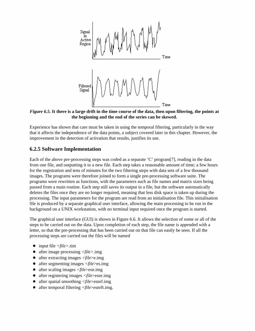
Figure 6.5. It there is a large drift in the time course of the data, then upon filtering, the points atthe beginning and the end of the series can be skewed.

Experience has shown that care must be taken in using the temporal filtering, particularly in the waythat it affects the independence of the data points, a subject covered later in this chapter. However, theimprovement in the detection of activation that results, justifies its use.

6.2.5 Software Implementation

Each of the above pre-processing steps was coded as a separate ’C’ program[7], reading in the datafrom one file, and outputting it to a new file. Each step takes a reasonable amount of time; a few hoursfor the registration and tens of minutes for the two filtering steps with data sets of a few thousandimages. The programs were therefore joined to form a single pre-processing software suite. Theprograms were rewritten as functions, with the parameters such as file names and matrix sizes beingpassed from a main routine. Each step still saves its output in a file, but the software automaticallydeletes the files once they are no longer required, meaning that less disk space is taken up during theprocessing. The input parameters for the program are read from an initialisation file. This initialisationfile is produced by a separate graphical user interface, allowing the main processing to be run in thebackground on a UNIX workstation, with no terminal input required once the program is started.

The graphical user interface (GUI) is shown in Figure 6.6. It allows the selection of some or all of thesteps to be carried out on the data. Upon completion of each step, the file name is appended with aletter, so that the pre-processing that has been carried out on that file can easily be seen. If all theprocessing steps are carried out the files will be named

input file <file> .tim after image processing <file> .img after extracting images <file>e.img after segmenting images <file>es.img after scaling images <file>esn.img after registering images <file>esnr.img after spatial smoothing <file>esnrf.img after temporal filtering <file>esnrft.img.

For any image files that are created, a header file compatible with the Analyze display software[8], isalso created. Other features of the GUI include the ability to start the processing at a later timespecified by the user, and the option to print out the settings used, which can be kept as a record. TheGUI was written in ’C’, using the xview, library routines. The time taken to pre-process fMRI data issignificantly reduced using the new software, largely because all the steps can be set off to run in a fewminutes, and allowed to run without the need for user interaction, overnight if necessary.

Figure 6.6 The front panel of the graphical user interface for the fMRI data pre-processing package.

The user instructions for the fMRI pre-processing package is included as Appendix B.

6.3 Statistical Analysis of the Data

Many techniques have been proposed for statistically analysing fMRI data, and a variety of these arein general use. The aim of such analysis is to produce an image identifying the regions which showsignificant signal change in response to the task. Each pixel is assigned a value dependent on thelikelihood of the null hypothesis, that the observed signal changes can be explained purely by randomvariation in the data consistent with its variance, being false. Such an image is called a statisticalparametric map. The aim of this section is to show how such maps can be produced.

All the methods described below have been used, at one time or another, in the analysis of the datapresented in this thesis. The majority have been implemented as ’C’ programs, with the notableexception of using the SPM[10] implementation of the general linear model.

Throughout this section, the analysis techniques described are demonstrated on an example data set.The experiment performed was intended to detect activations resulting from a visually cued motortask. The whole brain of the subject was imaged, in 16 coronal slices of resolution 3 x 3 x 10 mm3,every four seconds. As cued by an LED display, they were required to squeeze a ball at the rate of 2Hz. The experiment involved 16 s of rest, followed by 16 s of task performance, repeated 32 times.

Further detail of the statistics mentioned in this chapter can be found in many statistics text books, forexample those by Zar[11], and Miller and Freund[12].

6.3.1 Subtraction Techniques

One of the simplest methods for obtaining results from a two state fMRI experiment is to perform asimple subtraction. This is carried out by averaging together all the images acquired during the ’on’phase of the task, and subtracting the average of all the ’off’ images. The disadvantage of such atechnique is that it is extremely sensitive to head motion, leading to large amounts of artefact in theimage. Figure 6.7a shows a single slice through the motor cortex from the example data set, and Figure6.7b shows the result of subtracting the ’off’ images from the ’on’ images. Although signal increasecan be seen in the primary motor cortex, there is also a large amount of artefact, particularly at theboundaries in the image.

Such a method does not yield a statistic that can be tested against the null hypothesis, so instead ofstraight subtraction it is more common to use a Student’s t-test. This weights the difference in means,by the standard deviation in ’off’ or ’on’ values, giving high t-scores to large differences with smallstandard deviations, and low t-scores to small differences with large standard deviations. The t-score iscalculated on a pixel by pixel basis, for a time series X, using the formula

(6.5)

where

(6.6)

and is the pooled variance

. (6.7)

The suffix ’1’ refers to the n1 images acquired during the ’on’ period of the task, and ’2’ refers to the n2 images acquired during the rest period. Figure 6.7c shows the statistical parametric map of t-scoresfor the sample data set. Again motor cortex activation is clearly seen, but the movement artefact isreduced compared to the subtraction technique.

(a) (b) (c)Figure 6.7 Use of subtraction techniques to analyse fMRI data. (a) A single slice coronal EPI

image through the primary motor cortex. (b) The mean of the images acquired during the ’off’period of the fMRI experiment subtracted from the mean of the images acquired during the ’on’

period. (c) The t-statistical parametric map corresponding to image (b).

6.3.2 Correlation techniques

Since we know that the BOLD response is mediated by blood flow, it is possible to improve thedetection of activations by predicting the shape of the response to the stimulus, and calculatingcorrelation coefficients between each pixel time course and this reference waveform. This is lesssensitive to other physiological changes during the experiment, and to movement. For a time course X,and a reference waveform Y, the correlation coefficient is calculated as

, (6.8)

and has a value of 1 for perfect correlation, a value of zero for no correlation, and a value of -1 forperfect anti-correlation.

The choice of an appropriate reference waveform is vital for the success of this technique in findingactivations. The first approximation might be a square wave, which is high for scans acquired duringthe task, and low for scans acquired during rest (Figure 6.8a). Such a waveform however takes noaccount of the delay and smoothness of the haemodynamic response which regulates the BOLDcontrast. An improvement to this would be to change the phase of the square wave (Figure 6.8b), withthe delay being between 3 and 6 seconds.

To improve the reference waveform further, it is necessary to look more closely at the actualhaemodynamic response. In an experiment such as the one used for the example data set, where thereis both visual and motor activation, it is possible to use the response to one type of stimulus to formthe reference waveform for finding the other. In this case the time series for one or more pixels in, saythe visual cortex is extracted (Figure 6.8c), and correlation coefficients are calculated between thiswaveform and that of every other pixel in the image. Such an analysis detects only those regions in thebrain which respond to the stimulus in the same way as the visual cortex. The major disadvantage ofthis technique is that it is particularly sensitive to motion artefact, since if such artefact is present in thereference waveform then the movement of other regions will be highly correlated. To attempt toreduce this, the response in the visual cortex to each stimulus can be averaged together, producing amean response to the single cycle. The reference waveform is then made up of a repetition of thesesingle cycle average responses (Figure 6.8d).

Figure 6.8. Various reference functions that can be used to correlate with a pixel time course todetect activations (see text for descriptions)

To be more general in predicting the haemodynamic response, so that a reference waveform can beconstructed for any length of stimulus, it is necessary to know the response to a single stimulus. Friston[13] suggested that a haemodynamic response function could be considered as a point spreadfunction, which smoothes and shifts the input function. By deconvolving the response from a knownarea of activation with the stimulus function, the haemodynamic response function can be obtained.The haemodynamic response function is not completely uniform across the entire brain however, andthe shape obtained from one region may not be optimum for another. As an alternative, the responsecan be modelled by a mathematical function, such as a Poisson or beta function. The Poisson function

(6.9)

with width l = 6 seconds, seems to fit well to observed haemodynamic responses (Figure 6.8e).

Since in general each slice of the volume imaged is not acquired at the same instant, it is necessary toaccommodate timing differences in the correlation with the reference waveform. In order to do this,the relative magnitude of the activation at the time each slice was acquired is predicted, by convolvingthe input stimulus with a Poisson function. Then from this series, the correlation coefficients can becalculated on a slice by slice basis, constructing the reference waveform from the appropriate points inthe predicted time series.

Examples of the effect of the reference waveform on the result is shown in Figure 6.9. Here, pixels inthe head which correlate to the reference waveforms (shown in Figure 6.8), with r > 0.20 are shown inred, on top of the base image. The square wave correlation is the least effective in detecting activations(a), however a considerable improvement is obtained by delaying the waveform by 4 seconds (b). Thecorrelation of the visual cortex with itself (c) is, not surprisingly, high, but using the average visualcortex response (d) improves the correlation in the motor cortex. The Poisson function model of thehaemodynamic response (e) improves slightly on the delayed square wave, and is a good model.

(a) Square wave

(b) Delayed Square Wave

(c) Visual Cortex Response

(d) Average Visual Cortex Response

(e) Poisson Distribution Model

Figure 6.9 Activation images obtained by correlating the test data sets with the referencewaveforms shown in Figure 6.8.

6.3.3 The General Linear Model

The statistical techniques described above are both parametric tests. That is to say, they assume thatthe observations are taken from normal populations. Most parametric modelling techniques are specialcases of the general linear model. This framework for analysing functional imaging data, firstdeveloped for PET and then extended for fMRI, is implemented in the software package SPM[14]. Thegeneral linear model is only outlined here, since the theory is extensively covered in the literature[15].

The aim of the general linear model is to explain the variation of the time course y1...yi...yn, in terms ofa linear combination of explanatory variables and an error term. For a simple model with only oneexplanatory variable x1...xi...xn, the general linear model can be written

(6.10)

where b is the scaling, or slope parameter, and ei is the error term. If the model includes more variablesit is convenient to write the general linear model in matrix form

, (6.11)

where now Y is the vector of observed pixel values, b is the vector of parameters and e is the vector oferror terms. The matrix X is known as the design matrix. It has one row for every time point in theoriginal data, and one column for every explanatory variable in the model. In analysing an fMRIexperiment, the columns of X contain vectors corresponding to the ’on’ and ’off’ elements of thestimulus presented. By finding the magnitude of the parameter in b corresponding to these vectors, thepresence or absence of activation can be detected.

b can be determined by solving the ’normal equations’

(6.12)

where is the best linear estimate of b. Provided that (XTX) is invertible then is given by

. (6.13)

Such parameter estimates are normally distributed, and since the error term can be determined,statistical inference can be made as to whether the b parameter corresponding to the model of anactivation response is significantly different from the null hypothesis.

The general linear model provides a framework for most kinds of modelling of the data, and caneliminate effects that may confound the analysis, such as drift or respiration, provided that they can bemodelled.

6.3.4 The Serial T-Test

All the techniques described above require the prediction of the time course that active regions willfollow. For many experiments, the use of rapid imaging, and carefully designed paradigms, makes theseparation of the order of cognitive events possible. One such example, which is part of our study ofParkinson’s disease and described in more detail in Chapter 7, is a paradigm involving the initiation ofmovement. In this experiment, the subject was required to respond, by pressing a hand held button, to

the visual presentation of the number ’5’, and to make no response to the presentation of a ’2’. Thisparadigm presented two differences to conventional, epoch based experiments. Firstly, the activationsof interest, which are those responsible for the button pressing, occurred at an irregular rate. Secondly,all the cognitive processes involved in the task, including both the planning and execution of themovement, occurred in a time period of a few hundred milliseconds, as opposed to the sustainedactivation used in epoch based paradigms. Such an experiment requires a new form of analysis. Twotechniques have been evaluated, both of which make no assumptions about the time course ofactivations during the task: the serial t-test, described here, and an analysis of variance technique,explained in the next section.

The basis of the serial t-test is to define a resting state baseline, and compare the images acquired ateach time point before, during and after the task with this baseline. Figure 6.10 illustrates thetechnique. For each time point following the stimulus, a mean and standard deviation image isconstructed, as is a baseline mean and standard deviation image. Then a set of t-statistical parametricmaps are formed by calculating, on a pixel by pixel basis, the t-score (using equations 6.5 - 6.7) for thedifference between mean image one and the mean baseline image, mean image two and baseline, andso on.

Figure 6.10. fMRI analysis using the serial t-test

Figure 6.11 shows the result of analysing the example data set using this technique. Such a data setdoes not really show the benefit of the serial t-test analysis. Results shown in Chapter 7 better illustrateits use in looking at event timings, and unpredictable waveforms.

Figure 6.11 Results of processing the test data set using the serial t-test. Eight volume image setsare shown as rows, the top four corresponding to the ’rest’ periods of the experiment, and the

next four corresponding to the ’task’ periods. Activation can be seen in both the primary motorand visual cortices.

The technique has two major disadvantages. The first is that, in order to achieve a sufficient signal tonoise ratio, it is necessary to have many more cycles than in an epoch based paradigm, thus leading tolonger experiments. This can be uncomfortable for the subject, and puts additional demands on thescanner hardware. There is some scope for bringing the single event tasks closer together, but theremust be a sufficient interval to allow the BOLD signal to return to baseline. This delay is at least tenseconds in length. The second disadvantage is that the analysis results in many statistical parametricmaps, which have to be interpreted as a whole. However the fact that the technique makes fewassumptions about the data time course makes it a strong technique, and opens up the possibility ofmore diverse experimental design, and a move away from the epoch based paradigms.

6.3.5 Analysis of Variance

A second technique which does not require any assumptions about the shape of the activation timecourse, looks at the changes in variance upon averaging. The technique is based on simple signalaveraging theory[16]. Take, for example, the response measured to a repeated signal as shown inFigure 6.12. The time series contains two components, one is a genuine response to the signal, and theother is the random fluctuations due to uncorrelated physiological events and noise in the image. Uponaveraging 32 cycles together, the magnitude of the noisy component is reduced but that of the repeatedsignal is not. The reduction of the noisy component can be measured by calculating the variance ofboth the unaveraged and averaged data set.

Figure 6.12. Signal Averaging. The variance of the noise in the average signal is N times less thanit is in the original signal, where N is the number of cycles.

To detect regions of activation, the ratio of the variance of the averaged data set to the variance of theunaveraged data set is calculated for each pixel in the image. For pixels in regions of purely randomintensity variations, this ratio will be around 1/n, where n is the number of cycles averaged together.Pixels in regions of activation, however, will have a significantly higher ratio than this, since thevariance of both unaveraged and averaged data sets is dominated by the stimulus locked intensityvariations of the BOLD effect, which does not reduce upon averaging.

The technique is more formally explained as an analysis of variance (ANOVA)[17]. If Xij refers to the ith time point after the stimulus, of the jth cycle of an experiment

time t X11, X12, ....., X1j, ....., X1n X1

time 2t X21, X22, ....., X2j, ....., X2n X2

........ ..... ..... ..... ..... ..... ..... .....

time it Xi1, Xi2, ....., Xij , ....., Xin X i

........ ..... ..... ..... ..... ..... ..... .....

time kt Xk1, Xk2, ....., Xkj, ....., Xkn Xk

X

with n cycles and k points per cycle. The null hypothesis is that there is no significant difference in the

means, . This can be tested by comparing two estimates of the population variance, s2, one basedon variations in measurements of the same time point, and one based on the variance between timepoints.

The variance within measurement of any time point can be calculated by

, (6.14)

and so the mean variance within time points is given by

, (6.15)

and is based on k(n-1) degrees of freedom. The variance of the time point means is given by

, (6.16)

and since

(6.17)

then s2 can be estimated by

(6.18)

which is based on k-1 degrees of freedom. Under the null hypothesis, both and independentlyestimate the population variance s2. This means that the ratio

(6.19)

will have an F distribution with k-1 and k(n-1) degrees of freedom. If there is any signal change that is

time locked to the stimulus, the value of will be larger than expected under the null hypothesis.

In the analysis of fMRI data, equations 6.15 - 6.19 are used to form an F-statistical parametric map.These equations are implemented using the following short-cut formulas

(6.20)

To assess the validity of this approach on real data, phantom and head images were analysed. Thephantom data set consisted of 256 volume images, each of 128 x 128 x 16 matrix size, obtained at arepetition rate of 4 seconds. The head data set consisted of 256 head images, of the same matrix size,with the subject performing no specified task. Both data sets were pre-processed in the same way thata functional imaging data set would be, and the analysis of variance was then carried out assuming 16points per cycle and 16 cycles. Histograms of F for each data set are shown in Figure 6.13, with theappropriate F distribution, shown as a dotted line, given by

(6.21)

where n1 is the number of points per cycle minus one, and n2 is the total number of data points minusthe number of points per cycle[18]. All three histograms show a good fit to the F distribution,confirming the validity of applying this technique to fMRI data.

(a)

(b)

(c)

Figure 6.13 Plots of calculated F-scores (solid line) and the appropriate F-distribution (dottedline) for (a) simulated data, (b) phantom data, and (c) head data.

The results of analysing the example activation data set using the ANOVA technique are shown inFigure 6.14. As with the serial t-test, such a data set does not best show the potential of this technique.A better example comes from the analysis of a study to investigate short term memory.

Figure 6.14 Results of processing the test data set using the analysis of variance technique. Thosepixels shaded in red correspond to regions which vary in some way that is time locked to the

stimulus.

The stimulus paradigm for this experiment had three stages. First three digits in succession werepresented to the subject. Eight seconds later a fourth digit was presented, and the subject was requiredto respond by pressing a button in their right hand if this final digit was the same as any of the threepreviously presented, or by pressing the button in their left hand if not[19]. The final stage was aperiod of rest, to provide a baseline. The whole test was repeated 32 times.

It would be expected that some regions of the brain would only be active during the presentation of thedigits, some during the retention period, some only in the recall stage and others throughout the wholememory task. To analyse such data using a correlation technique would mean predicting a whole set ofreference waveforms. The ANOVA technique, however, detected the responses of different shapes inone test. Figure 6.15 shows the activation maps obtained from the ANOVA analysis of the short termmemory experiment, together with time course plots from several of the areas.

Figure 6.15 Analysis of Variance technique applied to data from the short term memoryexperiment described in the text, together with average cycle plots for several regions of interest.Areas of the brain which act in different ways to the stimulus can be seen in a single activation

image.

The final image of an ANOVA analysis, essentially shows all the regions which vary in some way thatis synchronous to the presentation of the stimulus. It is equally good at picking up deactivations asactivations. This makes these images a good starting point for other forms of analysis, such asprincipal component analysis or cluster analysis, so as to glean all the information that is available.

6.3.6 Software Implementation

Due to the diversity of tests that can be carried out on one data set, software for implementing the testsdescribed above was written as a set of separate programs.

The program correlate constructs a reference waveform, from user specified values, and optionallyconvolves this with a Poisson function of user specified width. Correlation coefficients are calculatedusing equation 6.8. If the reference waveform is made to vary between 0 and 1 then a measure of thepercentage change upon activation can be obtained by calculating a linear regression of the form

where

(6.22)

and

.

The percentage change can be calculated as (b/a) x 100%.

The software also calculates the appropriate image of z-scores using Fishers Z transform and thereduced degrees of freedom as explained in the following sections. The file names for each of theseoutputs is

cc_<file> .img correlation coefficients saved as ’shorts’ x 10,000

pc_<file> .imgpercentage change saved as ’shorts’ x 1,000 (such that 1% signal change x 1,000)

cz_<file>. img z-scores saved as ’floats’ (not scaled)

The serial t-tests are performed by tmap and tmapnc, the first appropriate for cyclic experiments andthe second for non-cyclic experiments. For the non-cyclic version the stimulus times are obtained froma text file, and both output t-score maps saved as ’shorts’, scaled by 1000, in a file named tt_<file> .img.

ANOVA tests are carried out by the programs anova, and anovanc, which both output f-scores scaledby 1000, in a file named va_<file> .img.

6.4 Statistical Inference

The statistical analysis techniques discussed in the last section all result in a statistical parametric map(SPM), where each pixel in the image is assigned a value based on the likelihood that the nullhypothesis is false. However for the localisation and comparison of brain function, what is required isan image which only highlights those pixels which can confidently be labelled as active. This is doneby thresholding the statistical parametric map.

6.4.1 Confidence levels for T-scores, Correlation Coefficients and F-scores

Before approaching the problem of the significance of whole images, it is necessary to consider thequestion of the confidence that can be placed in the result of a single t-test, correlation or ANOVA.Such levels come from an understanding of the distribution, under the null hypothesis, of the statisticbeing considered. If for example a statistic had a normal distribution, as shown in Figure 6.16, acritical value Za can be defined such that

. (6.23)

Figure 6.16. The area under a normal distribution between Z0.005 and Zinf is 0.5% that of thetotal area under the curve.

This means that if the value of Z obtained in the statistical calculation is greater than Z0.005, we can be99.5% confident the null hypothesis is false. The number 0.005 in such a case is said to be the p-valuefor that particular test. Such values are tabulated in standard statistical texts, or can be obtaineddirectly from expressions for the distributions themselves.

The distribution for a correlation coefficient is dependent on the number of degrees of freedom in thetime course being analysed. For a time course of n independent time points, there are n-2 degrees offreedom. The question of whether time points from an fMRI experiment are independent is addressedlater in this section. The correlation coefficient, r, can be transformed so that it has a Z distribution(that is a Gaussian distribution with zero mean and unit variance), by applying the Fisher Z transform

. (6.24)

This transform may therefore be applied to the SPM of correlation coefficients, yielding an SPM of zscores.

The theory of Gaussian random fields (as described later, in section 6.4.3), applies to images of zscores. Therefore it is necessary to transform the t and f scores to z scores as well. This is done bycalculating the area under the distribution (p value) between t and infinity (or f and infinity), andchoosing an appropriate value of z such that the area under the Z distribution between z and infinity isthe same.

P-values for the t-statistic are related to the incomplete beta function

(6.25)

such that

(6.26)

where n is the number of degrees of freedom, which is equal to the number of data points that wereused to construct the statistic minus one.

Similarly p-values for the f-statistic can be derived from

(6.27)

where n1 is the number of points per cycles minus one and n2 is the total number of points minus thenumber of points per cycle (n1=k-1, n2=k(n-1)).

The transforms are carried out using pre defined functions in the package MATLAB[20], to calculatethe incomplete beta function and the inverse error function.

6.4.2 The Effect of Temporal Smoothing on Degrees of Freedom

All the statistical tests assume that the data points are independent samples of the underlyingpopulation. This however may not be the case, since the effect of the haemodynamic responsefunction, and any temporal smoothing that is applied to the data, means that adjacent time points areno longer independent. This has an effect on the effective number of degrees of freedom in the sample.

A detailed analysis of this problem is given in by Friston et. al.[21-23], but a more intuitiveexplanation of his result is given here.

Consider a series of n independent observations of a population of mean m.

The variance of the population is given by

(6.28)

which is best estimated by the sample variance

. (6.29)

The denominator in this expression is the number of degrees of freedom of the sample, and is one lessthan the number of observations, since only n-1 points are needed to describe the sample, the ’last’point being determined by the mean.

Now if the above data set is smoothed with a three point running filter such that

.

The sum of the square deviations from the mean of the data is now (on average) three times less thanthat of the unsmoothed data. This means that the population variance is now best approximated by

(6.30)

and implying that the smoothed data set has (n-1)/3 degrees of freedom. In the case of thepre-processing described above, the smoothing filter is a Gaussian kernel, as opposed to the three pointrunning average.

In this case it is necessary to evaluate the effect of neighbouring data points on any one point, and sothe reduction in the number of degrees of freedom is given by the area under the Gaussian kernel. Thenumber of degrees of freedom in the sample variance for a data set of n sample points, smoothed witha Gaussian of standard deviation s is therefore

. (6.31)

Simulations of the effect of smoothing data before carrying out an analysis of variance calculationshow that such a degrees of freedom reduction does not hold in this case. Temporal smoothing of thedata is unlikely to improve the ability of the ANOVA test to detect activations, and is therefore bestnot applied, however high pass filtering is likely to improve the test and should still be used.

A summary of the number of degrees of freedom for the tests described earlier is given below.

6.4.3 The Multiple Comparisons Problem and the Theory of Gaussian Random Fields

All the reasoning so far in this section is to do with the p values concerned with one statistical test.That is to say, for one individual pixel, we can be confident to a certain value of p, that its time courseis correlated to the stimulus. When we form an image from the results of such statistical tests, it isnecessary to consider how confident we are that none of the pixel labelled as ’active’, are in fact due torandom fluctuations. Take for example the SPM shown in Figure 6.17.

Figure 6.17 A 10 x 10 pixel matrix, with pixels shaded if they are shown to be ’active’ by somestatistical test with p>0.1

Here a pixel is shaded if a statistical test shows that the pixel is active, with a p value greater than 0.1.Since there are 100 pixels in the image, it is probable that 10 pixels will, by chance, be falsely labelledas active. The p value for such an image would therefore be 1.0, that is to say that we are certain that atleast one of the pixels is falsely labelled. This situation is called the multiple comparisons problem,and is well studied in statistics[24].

If all the pixels can be considered to be independent, then a Bonferroni correction can be applied. Thisstates that for an image of N pixels, the overall probability of any false positive result is P, if theindividual pixel false positive probability is P/N. However with thousands of pixels in an image, sucha technique is very stringent, and the risk of falsely rejecting true activations is very high. There is alsothe question of whether each pixel in the image can truly be regarded as independent. The point spreadfunction of the imaging process means that adjacent pixels cannot vary independently, and thissituation is worse if additional smoothing is applied.

Such problems were first addressed in PET data analysis, and the results carried over to fMRI. Thetheory of Gaussian random fields[25], was developed for the analysis of functional imaging data byFriston et. al.[26] and an overview of their important results is presented here.

For a completely random, D-dimensional, z-statistical parametric map consisting of S pixels, theexpected number of pixels that are greater than a particular z score threshold, u, is given by

. (6.32)

This is the area under the Gaussian distribution as shown in Figure 6.16. The theory attempts toestimate the number of discrete regions there will be above this threshold. Take for example the SPMshown in Figure 6.18a. This is formed from a simulated data set with completely independent pixels.

Those pixels with z-scores above a certain threshold are shown in white with those lower in black. Thesame data set, spatially smoothed before analysis is shown in Figure 6.18b. The number of whitepixels in each SPM is about the same, but the number of discrete regions of white pixels is much lessin the smooth case.

(a) (b)Figure 6.18. Two SPM’s thresholded at the same Z-score. (a) Values obtained from unsmoothed

data. (b) Values obtained from smoothed data

The expected number of regions appearing above u is estimated by

(6.33)

where W is a measure of the ’smoothness’, or resolution of the map. This is obtained by measuring thevariance of the first derivative of the SPM along each of the dimensions

. (6.34)

The average size of a region is thus given by

. (6.35)

Once these quantities have been estimated, the question is, what is the probability that a region (ofactivation) above a certain threshold u of size k pixels, could occur purely by chance. If k is of theorder of E{n} then this probability is quite high, but if k»E{n} then the probability reduces. The formof this probability distribution is taken as

(6.36)

where nmax is the size of the maximum region above u, in a random SPM, and

. (6.37)

Thus for a given SPM the smoothness parameter W can be calculated, and only those regions above achosen value of u that are of size greater than a chosen k are shown, the p value for the activationimage can be calculated using equations 6.32 - 6.37.

6.4.4 Image Presentation and Inter Subject Comparisons

Having thresholded the SPM to display only those ’active’ regions, these regions must besuperimposed on background images to enable anatomical localisation. If the EPI images that thefMRI data comes from are of suitable quality, then these can be used as the base images. Bettercontrast may come from some inversion recovery images (see Section 2.4.1) showing only whitematter, or grey matter. This is the practice used for the images shown in Chapter 7, and has theadvantage that any distortions in the images will be the same for both activation and background, andno image realignment is needed. Higher resolution EPI images with equal distortion can be obtainedusing interleaved EPI as discussed in Chapter 5. To obtain really high quality base images it isnecessary to use a 2DFT technique, however the distortions in such an image will be much less thanthe EPI functional images, and some form of alignment and ’warping’ is required in this case.

The subject of comparing results from a number of different experiments, either on the same person atdifferent times, or between different people, raises many issues, only a few of which are covered here.

Qualitative comparisons between subjects can be made by a good radiologist, familiar with EPIimages, however in order to quantify differences it is necessary to try and ’normalise’ the differencesbetween the brains of the subjects. This has traditionally been done in functional imaging by using theatlas of Talairach and Tournoux[27], based on slices from the brain of a single person. It uses aproportional grid system based on the location of two anatomical landmarks, the Anterior Commissure(AC) and the Posterior Commissure (PC). Having identified the locations of the AC, PC, and thesuperior, inferior, left, right, anterior and posterior edges of the brain, these co-ordinates are rotateduntil the line joining the AC and PC is along the x axis, and the line joining the left and right markersis parallel to the z axis (Figure 6.19).

Figure 6.19 Co-ordinate system in the transformation to Talairach space

The same rotations are performed on any ’activation’ region, and the co-ordinates are then scaled togive a distance in millimetres from the AC in each dimension, such that

AC - PC = 23 mm AC - Anterior = 70 mm AC - Posterior = 102 mm AC - Superior = 74.5 mm

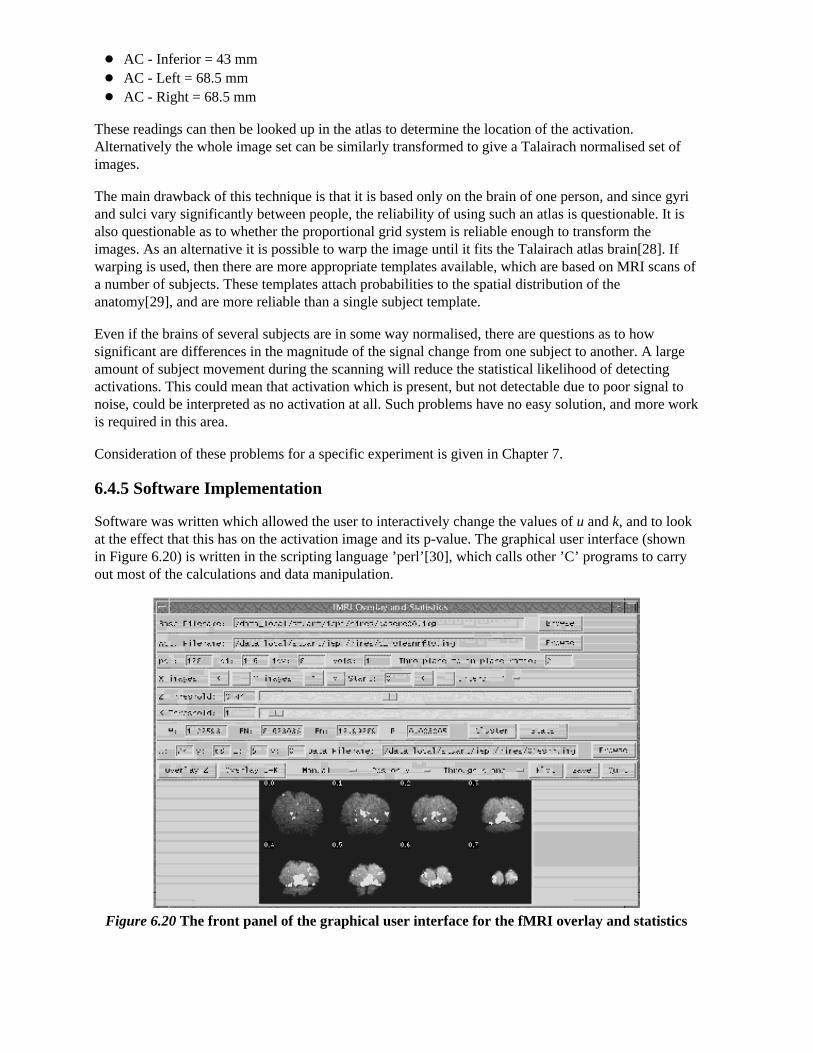
AC - Inferior = 43 mm AC - Left = 68.5 mm AC - Right = 68.5 mm

These readings can then be looked up in the atlas to determine the location of the activation.Alternatively the whole image set can be similarly transformed to give a Talairach normalised set ofimages.

The main drawback of this technique is that it is based only on the brain of one person, and since gyriand sulci vary significantly between people, the reliability of using such an atlas is questionable. It isalso questionable as to whether the proportional grid system is reliable enough to transform theimages. As an alternative it is possible to warp the image until it fits the Talairach atlas brain[28]. Ifwarping is used, then there are more appropriate templates available, which are based on MRI scans ofa number of subjects. These templates attach probabilities to the spatial distribution of the anatomy[29], and are more reliable than a single subject template.

Even if the brains of several subjects are in some way normalised, there are questions as to howsignificant are differences in the magnitude of the signal change from one subject to another. A largeamount of subject movement during the scanning will reduce the statistical likelihood of detectingactivations. This could mean that activation which is present, but not detectable due to poor signal tonoise, could be interpreted as no activation at all. Such problems have no easy solution, and more workis required in this area.

Consideration of these problems for a specific experiment is given in Chapter 7.

6.4.5 Software Implementation

Software was written which allowed the user to interactively change the values of u and k, and to lookat the effect that this has on the activation image and its p-value. The graphical user interface (shownin Figure 6.20) is written in the scripting language ’perl’[30], which calls other ’C’ programs to carryout most of the calculations and data manipulation.

Figure 6.20 The front panel of the graphical user interface for the fMRI overlay and statistics

software.y

SPMs of z-scores, stored as floats, are read in and thresholded at a z-score specified by a slider. Theseare displayed as white pixels, above a greyscale base image. The user can choose an appropriatecluster size threshold by either changing the slider or clicking on one of the regions with the mouse,and asking for the calculation of the size of that cluster. The activation image, with both thresholdsapplied can be displayed, and the p-value for such a combination calculated. It is necessary to changeboth thresholds interactively to find the optimum activation image for a given p-value, however resultsfrom Friston[31] suggest that wide signals are best detected using low z-thresholds and sharp signalswith high z-thresholds.

The time course plots for any selected region can be displayed, with the ’plot’ option. Any file can bechosen to take the plot intensities from, allowing the whole experiment time course, the average forone cycle, or Fourier components for the region to be displayed, provided that an image file containingsuch data exists.

Having chosen an appropriate set of thresholds, the images can be saved for display. The ’save’ optionallows any image file to be overlaid upon the base file, masked by the thresholded SPM. The baseimages are scaled between 0 and 20,000, and the ’active’ regions scaled between 20,000 and 32,000,which allows an appropriate image viewing package to display the base images in greyscale and theactivation in colour-scale. If the statistic used is also a good indicator of the magnitude of activationsignal change, for example the t-statistic for the difference between ’rest’ and activity, then it isappropriate to display in colour-scale the pixel values from the SPM. However for statistics such as thecorrelation coefficient, the values do not represent the amount of signal change. In these cases it ismore appropriate to display values from a percentage change image in colour, masked by thethresholded SPM. In order to appropriately identify the anatomical location of the activation, it issometimes desirable to see the brain structure that underlies the activation. In this case it is appropriateto use the base images as the source of the values for the activation regions. This means that the effectcan be created where the background image is in greyscale, and the active regions are ’shaded’ inred-scale. Examples of overlaying SPMs, regressions and base sets are shown in Figure 6.21.

(a)

(b)

(c)

Figure 6.21 Three ways of presenting the final results of an fMRI experiment. (a) Active regionsare shown in colour scale, with the colour (red to yellow) being determined by the magnitude ofvalues from the statistical parametric map. (b) The colour scale represents the percentage signal

change in that voxel upon activation. (c) The active regions are displayed as the red shadedregions of the base image set.

The software can also calculate the Talairach co-ordinates of any region, provided that the appropriatelandmarks can be identified (or deduced) from the images. Having entered the co-ordinates of thelandmarks, and chosen a region of interest, the co-ordinate system is rotated and proportionated, togive the distances in millimetres from the Anterior Commissure, of the centre of mass of that region inTalairach space.

The user instructions for the software is included as Appendix C.

6.5 Summary

The most important aspects of fMRI data analysis, as used on the data in this thesis have beenpresented above. The pre-processing steps improve the ability of the statistical analysis to detectactivations. The choice of an appropriate statistical test depends on the assumptions that can bereasonably made, and the questions that need to be addressed. Decisions about the statisticalsignificance of the results must take into account the multiple comparisons problem, and the reductionin degrees of freedom resulting from smoothing. Finally the results must be presented in anappropriate form, to enable the comparison of results between subjects.

In the whole process, many informed decisions need to be made, and it is difficult to propose a single’black box’ approach to the analysis, where data is fed in and an activation image is automatically fedout. However in order to formalise the analysis procedure to some degree, a standard analysis protocolwas written. This is included as Appendix D.

There are many more issues in the analysis that have not been mentioned here, and much work thatcan be done. For example the Fourier Analysis methods for detecting periodic activations[32] ,principal component analysis[33], clustering techniques which detect clump together pixels havingtime courses which vary in the same way, and nonparametric tests[34]. There are other methods forsolving the multiple comparison problem [35] and for carrying out inter subject comparisons. It is thislast area which requires the most attention, since, as fMRI becomes more and more a tool forneurologists to detect abnormality in brain function, the reliability of inter subject comparisons willbecome more important. It has been well shown that fMRI can give colourful pictures of the brainworking, and it is necessary to take the techniques for data analysis onward if fMRI is to fulfil itsclinical and neurological research potential.

6.6 References

[1]four1() from Press, W. H., Teukolsky, S. A., Vetterling, W. T. and Flannery B. P. (1992)‘Numerical Recipes in C’, Cambridge University Press.

[2] The motion correction software described was written by Dr. A. Martel, Department of MedicalPhysics, University of Nottingham.

[3] Hu, X., Le, T. H., Parrish, T. and Erhard, P. (1995) Retrospective Estimation and Correction ofPhysiological Fluctuation in Functional MRI. Magn. Reson. Med. 34,201-212.

[4] Friston, K. J., Williams, S., Howard, R., Frackowiak, R. S. J and Turner, R. (1996)Movement-Related Effects in fMRI Time-Series. Magn. Reson. Med. 35,346-355.

[5] Oppenheim, A. V. (1978) ‘Applications of Digital Signal Processing’, Prentice Hall.

[6] Friston, K. J., Holmes, A. P., Poline, J.-B., Grasby, P. J., Williams, S. C. R., Frackowiak, R. S. J.and Turner, R. (1995) Analysis of fMRI Time-Series Revisited. Neuroimage 2,45-53.

[7] See Kernighan, B. W. and Ritchie, D. M. (1978) ‘The C Programming Language’, Prentice-Hall.

[8] Analyze. Biomedical Imaging Resource, Mayo Foundation.

[9] Bandettini, P. A, Jesmanowicz, A., Wong, E. C. and Hyde, J. S. (1993) Processing Strategies forTime-Course Data Sets in Functional MRI of the Human Brain. Magn. Reson. Med. 30,161-173.

[10] SPM from the Wellcome Department of Cognitive Neurology http://www.fil.ion.ucl.ac.uk/SPM.

[11] Zar, J. H. (1996) ‘Biostatistical Analysis’, Prentice-Hall.

[12] Miller, I. and Freund, J. E. (1977) ‘Probability and Statistics for Engineers’, Prentice-Hall.

[13] Friston, K. J., Jezzard, P. and Turner, R. (1994) Analysis of Functional MRI Time-Series. HumanBrain Mapping 1,153-171.

[14] SPM from the Wellcome Department of Cognitive Neurology http://www.fil.ion.ucl.ac.uk/SPM.

[15] Friston, K. J., Holmes, A. P., Worsley, K. J., Poline, J.-B., Frith, C. D. and Frackowiak, R. S. J.(1995) Statistical Parametric Maps in Functional Imaging - A General Linear Approach. Human Brain Mapping 2,189-210.

[16]Lynn, P. A. (1989) ‘An Introduction to the Analysis and Processing of Signals’. Macmillan.

[17] Guenther, W. C. (1964) ‘Analysis of Variance’. Prentice-Hall.

[18] Mood, A. M. and Graybill, F. A. (1963) ‘Introduction to the Theory of Statistics’. McGraw-Hill,Second Edition p232.

[19] Hykin, J., Clare, S., Bowtell, R. Humberstone, M., Coxon, R., Worthington, B., Blumhardt, L. D.and Morris, P. A Non-directed Method in the Analysis of Functional Magnetic Resonance Imaging(fMRI) and it’s Application to Studies of Short Term Memory in Book of Abstracts, 13th AnnualMeeting, European Society of Magnetic Resonance in Medicine and Biology 366.

[20] MATLAB. The Math Works, Inc.

[21] Friston, K. J., Jezzard, P. and Turner, R. (1994) Analysis of Functional MRI Time-Series HumanBrain Mapping 1,153-171.

[22] Friston, K. J., Holmes, A. P., Poline, J.-B., Grasby, P. J., Williams, S. C. R., Frackowiak, R. S. J.and Turner, R. (1995) Analysis of fMRI Time-Series Revisited Neuroimage 2,45-53.

[23] Worsley, K. J. and Friston, K. J. (1995) Analysis of fMRI Time-Series Revisited - Again Neuroimage 2,173-181.

[24] Zar, J. H. (1996) ‘Biostatistical Analysis’, Prentice-Hall. p.211.

[25] Cox, D. R. and Miller, H. D. (1990) ‘The Theory of Stochastic Processes’, Chapman and Hall.

[26] Friston, K. J., Frith, C. D., Liddle, P. F. and Frackowiak, R. S. J. (1991) Comparing functional(PET) images: The assessment of significant change. J. Cereb. Blood Flow Metab. 11,690-699.

[27] Talairach, J. and Tournoux, P. (1988) ‘Co-planar Stereotaxic Atlas of the Human Brain’, Thieme.

[28] Collins, D. L., Neelin, P., Peters, T. M. and Evans, A. C. (1994) Automatic 3D IntersubjectRegistration of MR Volumetric Data in Standardized Talairach Space. J. Comput. Assist. Tomogr. 18,192-205.

[29] Mazziotta, J. C., Toga, A. W., Evans, A., Fox, P. and Lancaster, J. (1995) A Probabilistic Atlas ofthe Human Brain: Theory and Rationale for its Development. Neuroimage 2,89-101.

[30] See Wall, L. and Schwartz, R. L. ‘Programming Perl’, O’Reilly & Associates.

[31] Friston, K. J., Worsley, K. J., Frackowiak, R. S. J., Mazziotta, J. C. and Evans, A. C. (1994)Assessing the Significance of Focal Activations Using their Spatial Extent Human Brain Mapping 1,214-220.

[32] Lange, N. and Zeger, S. L. (1997) Non-linear Fourier Time Series Analysis for Human BrainMapping by Functional Magnetic Resonance Imaging. Applied Statist. 46,1-29.

[33] Backfrieder, W., Baumgartner, R., Sámal, M., Moser, E. and Bergmann, H. (1996) Quantificationof Intensity Variations in Functional MR Images Using Rotated Principal Components. Phys. Med. Biol. 41,1425-1438.

[34] Holmes, A. P., Blair, R. C., Watson, J. D. G. and Ford, I. (1996) Nonparametric Analysis ofStatistic Images from Functional Mapping Experiments. J. Cereb. Blood Flow Metab.16,7-22.

[35] Forman, S. D, Cohen, J. D., Fitzgerald, M., Eddy, W. F., Mintun, M. A. and Noll, D. C. (1995)Improved Assessment of Significant Activation in Functional Magnetic Resonance Imaging (fMRI):Use of a Cluster-Size Threshold. Magn. Reson. Med. 33,636-647.

Chapter 7 - Functional MRI of Motor Function

7.1 Introduction

The ability to control our movement is something that most of us take for granted. From the swiftresponses required to hit a cricket ball, to the delicate and steady action of surgeon, the brain is able tocontrol the muscles in the body in a precise and efficient way. Motor function is controlled by fourmajor regions in the frontal lobes; the primary motor cortex, supplementary motor area (SMA), lateralpremotor cortex and the cingulate motor area (shown in Figure 7.1). The primary motor cortex isresponsible for the direct production of movements via it’s outputs to the pyramidal tract, and damageto these areas resulting from stroke produces a weakness in the corresponding part of the body. Theother three areas are responsible for higher order control of motor function.

Figure 7.1 Locations of the primary motor cortex, premotor cortex and supplementary motor area.

Studies of the SMA using PET have shown that the it is involved in motor task sequencing andmovement initiation [1], however it has more recently been suggested on the basis of animal studiesthat the SMA could be divided into two discrete areas; the preSMA and the SMA proper [2]. TheSMA proper, projecting to and receiving inputs from the primary motor cortex, it is suggested is moredirectly responsible for movement execution, whereas the pre-SMA, receiving inputs from theprefrontal cortex and the cingulate motor areas, might be responsible for movement decision making.

In order to test this hypothesis on humans, using fMRI, it was necessary to use an experiment thatallows the elements of decision making and movement to be separated. Such an experiment would bedifficult to carry out in a standard epoch based paradigm with activation lasting for a number ofseconds. This would require a number of movement decision making tasks to be carried out in eachepoch, and separation of the areas responsible for the execution of the movement from thoseresponsible for the decision making would be impossible. Instead of this, single event paradigms weredeveloped, where one movement decision task was performed every 20 seconds or so, allowingdiscrimination between areas activated when the decision to move was made and those activated whenthe decision not to move was made.

In this study the paradigm design, subject handling and data analysis and inference was carried out byDr. Miles Humberstone [3].

7.2 Methods

7.2.1 Stimulus Presentation

For most paradigms involving the motor cortex, it is necessary to provide some form of cue to thesubject to move and, in most cases, a measurement of the movement made.

All our studies involve hand movements since these are the simplest to measure. The cue to move wasgiven from a 6 cm single digit LED display, as sketched in Figure 7.2.

Figure 7.2 Sketch of the single digit display used to present visual cues to the subject.

This allowed the presentation of symbols, individual bars or the dot as well as numbers. To measureresponse times the subject was given two hand held buttons, one for the left hand and one for the righthand, operated by a thumb press. A schematic diagram of the stimulus rig is shown in Figure 7.3.

Figure 7.3 Schematic diagram of stimulus presentation equipment.

The experiment was controlled by a PC fitted with an interfacing card [4]. This card had a number ofanalogue input and output ports, 18 digital lines that could be configured in ports of eight to be eitherinput or output, and three counter-timers. The card produced a 5 V D.C. power supply, which was notenough to drive the LED’s, so a Darlington driver IC was used as a buffer to provide the 12 Vrequired. The hand held buttons consisted of a 10 cm tube with a micro-switch mounted on the top.The switch required little force to depress and travelled a couple of millimetres. It had a clear actionhowever, so that the subject would know they had pressed it. The switch formed part of a circuit thatheld the digital input line to the interfacing card at ground normally, and to 5 V when depressed. A 5ms TTL trigger from the scanner was obtained for every scan, and this fed to one of the digital inputlines on interfacing card.

The counters on the card were arranged in a cascade. Counter 1 received triggers from the PC’sinternal clock at the rate of 2 MHz, and was set to output one pulse every 2000 triggers, that is everymillisecond.

This millisecond trigger was sent to the second counter, which was set to count to 1000, therebyproducing a trigger every second.

Counter 3 received this signal and counted to its limit (60,000). Thus any length of time could bemeasured to a accuracy of milliseconds by reading counters 2 and 3 (see Figure 7.4).

Figure 7.4. Cascading three counters to count in milliseconds and seconds.

The software to control the stimulus was written in ’C’ [5]. The general flow of programs consisted ofa loop to count over the cycles, loops to count over the number of stimuli presented per cycle and aloop to repeatedly monitor the scanner triggers, counters and subject buttons. Figure 7.5 shows anexample flow diagram for an experiment that presented a 200 ms visual cue every 10 scans andmeasured the time it took the subject to respond by pressing the button. In this example there are 50

scans of activity and 50 scans of rest, repeated 10 times. Other experiments were programmed in asimilar way. Triggering the experiment from the scanner ensured that there were no timing errors. Theresponse times were stored in a data file on the computer for later analysis if required.

The display and buttons could be connected locally to the computer, for testing and subject practice,and connected remotely during the scanning itself. The single digit display was mounted on a plasticsupport inside the scanner, about 50 cm away from the subjects face.

Figure 7.5. Example flow diagram of software to control stimulus presentation and measurereaction times, kept in pace by triggers from the scanner.

7.2.2 Paradigm Development

The initial basis of the paradigm used came from electrophysiological experiments. The oddballparadigm consists of the regular presentation of a stimulus, for example the visual presentation of thedigit ’2’, and infrequently presenting an ’oddball’ stimulus such as a ’5’. On the presentation of the ’5’the subject is required to respond by pressing a button. Regardless of the form the cue stimulus takes,EEG signals from a subject carrying out such a task reveal a peak with a latency of 300 ms, labelledthe P300, in response to every oddball stimulus [6].

The implementation of this paradigm for fMRI involved presenting the digits using the LED displaydescribed above, at a rate of 2 Hz, with the oddball stimulus occurring at a pseudo-random interval ofaverage 12 s. Analysis of the brain activation of the oddball responses, compared to the interval inbetween, should reveal those areas involved directly in the movement, including the SMA.

A slight change to the paradigm enabled discrimination between areas involved in the movementdecision making and those involved more directly in the movement itself. If the stimuli are presentedat a less frequent rate (one every 18 seconds) and the ’2’ or ’5’ presented with equal probability, theparadigm is of the form of a ’go, no-go’ experiment [7]. The subject again responds only to the ’5’, butthe brain response to the ’2’ will reveal areas responsible for the movement decision making process.The use of the digits ’2’ and ’5’ on the LED display make the stimuli symmetrical and of equalluminance. In total 50 stimuli were presented, with equal numbers of go and no-go stimuli presented inpseudo-random order. Six normal volunteers were studied using the ’go, no-go’ paradigm.

7.2.3 Imaging

The imaging for this experiment was carried out on a dedicated EPI scanner [8]. The static 3.0 Teslafield was produced by a superconducting magnet (Oxford Magnet Technology).

The gradient coils were designed for high uniformity, low heating and high efficiency, especially inthe z-axis [9]. The efficiencies of the three axis are: Gx = 0.087 mTm-1A -1; Gy = 0.087 mTm-1A -1;Gz = 0.35 mTm-1A -1. Due to its high efficiency, the z-axis gradient coil was used as the switchedaxis. This coil was driven as part of a tuned resonant circuit at a frequency of 1.9 kHz, by a bank of 8power amplifiers (Techron) connected in parallel. The blipped and slice select gradients were drivenby 2 and 6 power amplifiers respectively.

A birdcage radiofrequency coil was used, to give the most uniform r.f. field over the whole volume ofthe brain. R.f. power amplification came from a 10 kW amplifier. Gradient and RF control is carriedout by a set of in-house built waveform synthesis modules. These are controlled by a UNIXworkstation (Sun Microsystems) via a VME bus [10].

For the motor function experiments there were two requirements of the scanning; whole brain imagingand fast repetition rate. The rate of scanning is largely limited by the heating of the gradient coils andthe rate that data can be processed and stored. Using a matrix size of 128 x 128, with an in-planeresolution of 3 x 3 mm2, had the advantage that the brain filled only half of the field of view, meaningthat the N/2 ghost did not overlap and interfere with the image (see section 4.3.1). The gradient heatingand rate of saving data limited the acquisition of images of this matrix size to four a second (TR = 250ms).

To improve the repetition rate, a matrix size with half as many lines (128 x 64) was used, allowing aTR of 150 ms if scanning continuously for less than 5 minutes and a TR of 187 ms for less than 30minutes continuous scanning. The other advantage of using the smaller matrix size is that the totalsampling time is reduced by half (from 33 to 16.5 ms), thereby doubling the frequency per point in the

broadening direction and halving the distortion (see section 5.3.1).

To cover the whole brain in 9 mm contiguous slices would take 2.4 seconds at the fastest repetitionrate (150 ms). To reduce the time taken to acquire each volume required a reduction in the number ofslices acquired, either by increasing the slice thickness or reducing the area of brain that is covered.Earlier experiments were carried out using thicker slices, or with volume repetition rates of greaterthan 2 seconds. When the regions of the brain that were of interest had been ascertained, the slicethickness was kept at 9 mm and 10 slices chosen that covered this region, reducing the volumerepetition rate to 1.5 seconds.

Anatomical reference images were obtained for each subject using the fast inversion recoverysequence described in section 4.4. Grey matter null images were obtained using an inversion time of1200 ms and white matter null images with an inversion time of 400 ms. The slice thickness wasreduced to 3 mm for these images and the slices acquired such that three of these images correspondedexactly to one of the functional images.

Various methods were used to restrain the subjects head during scanning. Polystyrene foam, wedgedbetween the perspex former of the r.f. coil and either side of the subjects head was effective butbecame uncomfortable after 10 minutes or so. In addition the subject could still move their headforward and backward. A more rigid restraint was also tried, with foam ended rods that went intoeither ear, and a bridge that went across the nose. This was hard to adjust, and extremelyuncomfortable for the subject after only a few minutes. The head was well restrained with this method,but the subjects often made deliberate movements during scanning to reduce discomfort.

A third and more successful method was to use inflatable sphygmomanometer cuffs either side of thehead. These could be inflated until the subject was comfortable but well restrained. An open-cellpolyurathane foam was used underneath the head which was softer and therefore more comfortablethan the polystyrene foam. Although the subject was free to move the head forward and backward, theincreased comfort attained made them less likely to move in this way. Representations of the threetypes of restraint are shown in Figure 7.6.

Figure 7.6 Three methods of subject restraint. (a) Polystyrene foam padding, (b) rigid headrestraint and (c) inflatable cuff.

7.2.4 Analysis

The data from this experiment were analysed using the methods described in Chapter 6. Registration,normalisation, spatial and temporal filtering were carried out using the pre-processing packagedescribed in section 6.2.

The statistical analysis used was a serial t-test (section 6.3.4), with a baseline period defined at 3 to 6seconds prior to the stimulus presentation. The responses to the ’go’ stimulus were processedseparately to the responses to the ’no-go’ stimuli, with any errors in the response excluded from theanalysis. This produced two sets of t-statistical parametric maps, which could be analysed using thetheory of Gaussian random fields (section 6.4.3).

The activation maps were interpolated up to 60 slices and superimposed directly on the inversionrecovery images, displayed as 3-D volumes to help anatomical localisation of the activated regions.Talairach co-ordinates were obtained for each active region.

For each subject the point in the time course of maximal activation in the rostral and caudal medialpremotor cortex was identified, and the percentage changes in response to the ’go’ and ’no-go’ tasksfrom the rest state measured. Similarly the points of maximal activity during the ’go’ and the ’no-go’task were identified in the primary motor cortex. Paired t-test comparisons between the ’go’ and’no-go’ percentage changes were performed across subjects for these regions of maximum activity.

7.3 Results

Figure 7.7 shows the activation at 0 s, 3 s, 6 s and 9 s following the stimulus, for one subject in the’go, no-go’ experiment. Maximum activation occurs at 3-6 seconds from the delivery of the stimulus.During the ’no-go’ task, activation was seen in the medial premotor cortex for all the subjects. Thisregion was rostral to the anterior commissural (AC) line. Activity was observed in these regions duringthe ’go’ task as well (see Figure 7.8). During the ’go’ task activation was also seen in a region of thepremotor cortex caudal to the AC line.

Figure 7.7 Volume images acquires between 0 and 12 seconds after the presentation of either a’go’ or ’no-go’ stimulus

Go No-Go

Figure 7.8 View of the medial surface of the left hemisphere, three seconds after the stimulus in ago, no-go paradigm.

The mean value of the percentage change upon activation of the areas involved in the motor task areshown in Figure 7.9. This shows the rostral part of the premotor cortex (labelled pre-SMA) to beactive in both ’go’ and ’no-go’ tasks, with the caudal part (labelled SMA) being only active in the ’go’task. This suggests that the pre-SMA is involved in the movement decision making aspect of the task,whereas the SMA proper is more intimately involved in the movement itself.

Figure 7.9 Plots of the percentage signal change in the Pre-SMA, SMA and primary motorcortex, for the ’go’ and the ’no-go’ task.

7.4 Discussion

The results presented illustrate that the imaging of single events is possible. As was mentioned earlier,such a study of movement decision making would be difficult to carry out using a traditional epochbased paradigm. From the electrophysiological measurements of such tasks, it is clear that the neuralactivity only lasts a few hundred milliseconds, however such short neural events can be detected usingfMRI. This is important since many other interesting cognitive paradigms do not adapt easily toproviding periods of sustained activity. Since similar techniques of stimulus presentation are used inbrain studies using evoked potentials, the same experiments can be used with both modalities.

Single event paradigms require longer experiments than their epoch based counterparts, in order thatthe required signal to noise ratio is achieved. A delay of at least 10 seconds is required between eachstimulus to enable the blood flow changes to return to the baseline.

7.5 References

[1] Passingham, R. (1993) ’The Frontal Lobes and Voluntary Action’. Oxford University Press.

[2] Matsuzaka, Y., Aizawa, H. and Tanji, J. (1992) A Motor Area Rostral to the Supplementary MotorArea (Presupplementary Motor Area) in the Monkey: Neuronal Activity During a Learned MotorTask. J. Neurophysiol. 68,653-662.

[3] Humberstone, M., Sawle, G. V., Clare, S., Hykin, J., Coxon, R., Bowtell, R., Macdonald, I. A. andMorris, P. (1997) Functional MRI of Single Motor Events Annals of Neurology In Press.

[4] Lab PC+, National Instruments Corporation.

[5] Turbo C++, Borland.

[6] Rohrbaugh, J. W., Parasuraman, R. and Johnson, R. (1990) ’Event-Related Brain Potentials’,Oxford University Press.

[7] Leimkuhler, M. E. and Mesulam, M. M. (1985) Reversible Go-No go Deficits in a Case of FrontalLobe Tumour. Ann. Neurol. 18,617-619.

[8] Mansfield, P., Coxon, R. and Glover, P. (1994) Echo-Planar Imaging of the Brain at 3.0 T: FirstNormal Volunteer Results. J. Comput. Assist. Tomogr. 18,339-343.

[9] Peters, A. M., Mansfield, P. and Bowtell, R. (1996) A short head gradient set for EPI at highmagnetic field. in Book of Abstracts, 13th Annual Meeting European Society of Magnetic Resonancein Medicine and Biology. Abstract 138.

[10] Glover, P. (1993) High Field Magnetic Resonance Imaging. PhD Thesis, University ofNottingham.

Chapter 8 - DiscussionAs was said at the start of this thesis, the field of fMRI is rapidly finding clinical application and isexciting scientists from a range of disciplines including neurologists, psychiatrists and psychologists.However, there is still much research and development that needs to be done on the technique itself.

The effect of echo time (TE) on the ability to detect signal change due to the BOLD effect is striking,in particular the lack of detectable BOLD contrast at low echo times (< 15 ms). The results from theecho time measurement experiment described in Chapter 4, that the most suitable echo time to use forfMRI of the auditory, visual or motor cortices 3.0 T being between 30 and 40 ms, takes some of theguess work out the choice of imaging parameters to use when engaging in a new fMRI study. Thereare other parameters that may also have a significant effect on the level of BOLD contrast, such asslice thickness, voxel size and repetition rate (TR), and these will need to be investigated. The singleshot T2

* measurement technique not only provides a quick and reliable way to find the optimum echo

time, but also provides a way to map the actual changes in T2* upon functional stimulation. This will

give a more direct handle on one of the effects of changes in blood oxygenation, and may prove usefulin determining the underlying mechanisms of the BOLD effect.

Image quality is always important in MRI, since artefact can be misleading to a clinician trying tointerpret results. The N/2 ghost is one of the most obvious artefacts in echo planar images, and itspresence not only spoils the appearance of the images, but can also prevent the detection of signalchanges due to the BOLD effect. The assessment of various methods for correcting this particularartefact in Chapter 4 suggested that the method by Buonocore, which does not require a referencescan, is the most appropriate to use on fMRI data. However this result will have to be verified by itsroutine use on ’real’ fMRI data sets. The second artefact correction technique described in Chapter 4,the removal of the effect of external r.f. interference, is purely cosmetic, however its use again meansthat the final activation images are clearer for clinical assessment.

The fast inversion recovery pulse sequence presented has enabled the reduction in the time a subjectspends in the scanner. Any such methods for reducing the experimental duration are desirable, notonly since they make precious scanner time more efficient, but also because subject discomfort isreduced. The standard experimental protocol, as given in Appendix A, and explained in Chapter 4,gives a framework to enable the consistent acquisition of fMRI data. The activation maps show a greatdeal of variability between subjects, and some variability within subjects scanned at different times,due to physiological effects, and so any standardising procedure that reduces variability in the way thatthe scanning is carried out is helpful. The protocol will need to be developed with time, as changes inscanner hardware and software are made, and as new information on optimum imaging parametersbecomes available.

The main conclusion from the experience of using interleaved EPI for high resolution fMRI, is thatmethods for correcting the effect of subject movement need to be developed if the technique is toprovide useful results. However the results that are shown in Chapter 5 indicate that effort in this areais worthwhile, since greater detail can be obtained from sub-millimetre resolution fMRI. In themeantime, the technique will be useful in reducing the distortion in activation images or for providinghigh resolution anatomical images with identical distortion to the overlaid activation maps.

The statistical analysis of fMRI data is being actively researched in many functional imaging centresand much effort is needed in this area. The new methods for the non-directed analysis of dataexplained in Chapter 6 offer the possibility of detecting regions of activation exhibiting many differenttime courses and allow the analysis of single event cognitive paradigms. More techniques of this kindare needed, all of which must be put on a firm statistical footing, and methods that are powerful in

detecting activations and statistically robust will find great application amongst clinicians not familiarwith the fMRI analysis. In the suite of programs that have been developed, and that are documented inChapter 6, a straightforward and minimal input way of analysing fMRI data has been offered.

The results presented in Chapter 7 show that single event functional imaging, where the subjectundertakes a single task, relatively infrequently, can yield important neurological results. Theseparation of motor planning events from execution has confirmed the sub-division of supplementarymotor area, and its role in motor function.

It has now been firmly established that magnetic resonance imaging can be used to map brain function.The main impetus of research and development of the technique, needs to be directed in several areasif fMRI is to become more than ’colour phrenology’, intriguing in its results yet having little clinicalvalue. The mechanisms behind the BOLD effect need to be better understood, as does thephysiological basis of the observed blood flow and oxygenation changes The combination of thefunctional imaging modalities needs attention, since it is unlikely that any one method will provide thefull picture. Finally, robust and simple techniques for data analysis need to be developed, allowingthose who do not specialise in fMRI, to carry out experiments and interpret results. All that said,functional MRI offers possibilities for basic neurological research and clinical application that couldnot have been imagined ten years ago, and I am sure that the next ten years will be just as exciting.