From Volatility Modelling to Structured ProductsPricing

Authors:SOULEYMANE DIEYEJULIEN MESSIAS

April 20, 2021

Contents

1 From Implied Volatility to Local Volatility Surface 5I Implied Volatility Surface . . . . . . . . . . . . . . . . . . . . . . . . . . . . . . . . . . . . . . . . . . . . . 5

I.1 Stochastic Volatility Inspired SVI . . . . . . . . . . . . . . . . . . . . . . . . . . . . . . . . . . . . 5I.1.1 Parameters interpretation . . . . . . . . . . . . . . . . . . . . . . . . . . . . . . . . . . . 6I.1.2 Model Properties . . . . . . . . . . . . . . . . . . . . . . . . . . . . . . . . . . . . . . . 7

I.2 Arbitrage-Free Conditions . . . . . . . . . . . . . . . . . . . . . . . . . . . . . . . . . . . . . . . . 7I.2.1 Calendar Spread Arbitrage . . . . . . . . . . . . . . . . . . . . . . . . . . . . . . . . . . 7I.2.2 Butterfly Arbitrage . . . . . . . . . . . . . . . . . . . . . . . . . . . . . . . . . . . . . . . 7

I.3 Problem Formulation - Calibration(s) . . . . . . . . . . . . . . . . . . . . . . . . . . . . . . . . . . 8I.3.1 Calendar Spread Arbitrage . . . . . . . . . . . . . . . . . . . . . . . . . . . . . . . . . . 8I.3.2 Butterfly Arbitrage . . . . . . . . . . . . . . . . . . . . . . . . . . . . . . . . . . . . . . . 8I.3.3 Optimization Problem . . . . . . . . . . . . . . . . . . . . . . . . . . . . . . . . . . . . . 9

II Skew and Term Structure . . . . . . . . . . . . . . . . . . . . . . . . . . . . . . . . . . . . . . . . . . . . . 9II.1 Skew . . . . . . . . . . . . . . . . . . . . . . . . . . . . . . . . . . . . . . . . . . . . . . . . . . . 9II.2 The Smile Curvature . . . . . . . . . . . . . . . . . . . . . . . . . . . . . . . . . . . . . . . . . . . 10II.3 Term Structure . . . . . . . . . . . . . . . . . . . . . . . . . . . . . . . . . . . . . . . . . . . . . . 10II.4 Stylized Facts . . . . . . . . . . . . . . . . . . . . . . . . . . . . . . . . . . . . . . . . . . . . . . . 10

III Implied Volatility for Long-Term Maturities . . . . . . . . . . . . . . . . . . . . . . . . . . . . . . . . . . . 11IV Local Volatility . . . . . . . . . . . . . . . . . . . . . . . . . . . . . . . . . . . . . . . . . . . . . . . . . . 11

IV.1 Derivation of the Dupire Equation . . . . . . . . . . . . . . . . . . . . . . . . . . . . . . . . . . . . 11IV.2 Local Volatility in terms of Implied Volatility . . . . . . . . . . . . . . . . . . . . . . . . . . . . . . 12

V Numerical Results . . . . . . . . . . . . . . . . . . . . . . . . . . . . . . . . . . . . . . . . . . . . . . . . . 13V.1 Calendar arbitrage . . . . . . . . . . . . . . . . . . . . . . . . . . . . . . . . . . . . . . . . . . . . 13V.2 Butterfly arbitrage . . . . . . . . . . . . . . . . . . . . . . . . . . . . . . . . . . . . . . . . . . . . 14V.3 Stylized Facts . . . . . . . . . . . . . . . . . . . . . . . . . . . . . . . . . . . . . . . . . . . . . . . 15V.4 error of estimations . . . . . . . . . . . . . . . . . . . . . . . . . . . . . . . . . . . . . . . . . . . . 16V.5 Local and Implied Volatility Surface . . . . . . . . . . . . . . . . . . . . . . . . . . . . . . . . . . . 17

2 Monte-Carlo Simulations and Model 18I Monte-Carlo Principle . . . . . . . . . . . . . . . . . . . . . . . . . . . . . . . . . . . . . . . . . . . . . . 18II Local Volatility Model and Mono-Asset Diffusion . . . . . . . . . . . . . . . . . . . . . . . . . . . . . . . . 19

II.1 Local Volatility Model . . . . . . . . . . . . . . . . . . . . . . . . . . . . . . . . . . . . . . . . . . 19II.2 Discretization . . . . . . . . . . . . . . . . . . . . . . . . . . . . . . . . . . . . . . . . . . . . . . . 19II.3 Discrete Dividend . . . . . . . . . . . . . . . . . . . . . . . . . . . . . . . . . . . . . . . . . . . . 19II.4 Local Volatility Interpolation . . . . . . . . . . . . . . . . . . . . . . . . . . . . . . . . . . . . . . . 20II.5 Convergence and Optimization . . . . . . . . . . . . . . . . . . . . . . . . . . . . . . . . . . . . . . 20

III Multi-dimensional Simulation . . . . . . . . . . . . . . . . . . . . . . . . . . . . . . . . . . . . . . . . . . 21IV Numerical Results . . . . . . . . . . . . . . . . . . . . . . . . . . . . . . . . . . . . . . . . . . . . . . . . . 22

IV.1 Correlation Multi-Assets . . . . . . . . . . . . . . . . . . . . . . . . . . . . . . . . . . . . . . . . . 22IV.2 Convergence of the Empirical mean of the stock Price to the Forward Price . . . . . . . . . . . . . . 23

1

3 Structured Products 25I Overview on structured products . . . . . . . . . . . . . . . . . . . . . . . . . . . . . . . . . . . . . . . . . 25II Autocall Athéna . . . . . . . . . . . . . . . . . . . . . . . . . . . . . . . . . . . . . . . . . . . . . . . . . . 26III Numerical Results . . . . . . . . . . . . . . . . . . . . . . . . . . . . . . . . . . . . . . . . . . . . . . . . . 28

III.1 Example of Athena . . . . . . . . . . . . . . . . . . . . . . . . . . . . . . . . . . . . . . . . . . . . 28III.2 The effect of Correlation on multi-asset options . . . . . . . . . . . . . . . . . . . . . . . . . . . . . 29

IV sensitivities and Hedging tools . . . . . . . . . . . . . . . . . . . . . . . . . . . . . . . . . . . . . . . . . . 29IV.1 sensitivities . . . . . . . . . . . . . . . . . . . . . . . . . . . . . . . . . . . . . . . . . . . . . . . . 29

IV.1.1 Dividend yield . . . . . . . . . . . . . . . . . . . . . . . . . . . . . . . . . . . . . . . . . 30IV.1.2 Implied volatility and skew . . . . . . . . . . . . . . . . . . . . . . . . . . . . . . . . . . 30IV.1.3 Issuer rating and default risk (funding risk) . . . . . . . . . . . . . . . . . . . . . . . . . . 30

IV.2 Hedging . . . . . . . . . . . . . . . . . . . . . . . . . . . . . . . . . . . . . . . . . . . . . . . . . . 31IV.2.1 Dividend yield . . . . . . . . . . . . . . . . . . . . . . . . . . . . . . . . . . . . . . . . . 31IV.2.2 Implied volatility and skew . . . . . . . . . . . . . . . . . . . . . . . . . . . . . . . . . . 31IV.2.3 Correlation . . . . . . . . . . . . . . . . . . . . . . . . . . . . . . . . . . . . . . . . . . . 32

2

Introduction

Structured products were first issued at the beginning of the last century, and were designed to address the specific needs ofconsumers in terms of payoff and exposure by allowing for a yield-enhancing approach. Unlike traditional Vanilla options,they have a number of features (coupon rate, triggers, etc.) that make them more difficult to value and hedge over theirlife cycle. Over the past fifteen years, the exotic derivatives industry has grown at a breakneck rate, with investment bankscontinuously innovating to satisfy ever-more-specific requests, tailor-made structured products are becoming commonplace.Furthermore, as a result of the financial crisis having an effect on investment mentalities and policies, “guaranteed capital”products now make up a large portion of the transactions.Structured Products can be valued as a combination of options but we prefered to use Monte-Carlo techniques for path-dependant products. All of this necessitates the use of efficient, appropriate algorithms and pricing tools. Various kinds ofmodels are utilized for pricing: every feature can be decisive in the models choice and an inappropriate choice may have animportant consequence on the valuation.

3

Data setsThe data used come, mainly, from Bloomberg. We did our study and tests based on 4 datasets :

• Data set 1: Euro Stoxx 50, on 2020-11-16

• Data set 2: Euro Stoxx 50, on 2020-12-08

• Data set 3: SP 500, on 2020-12-09

• Data set 4: Nasdaq 100, on 2020-12-31

Each data set is composed of :

• implied volatitilities extracted directly, i.e we used the implied volatility generated by Bloomberg, trusting the methodused by Bloomberg, which used a binomial tree method to invert the price towards the volatility. We get all the impliedvolatilities of the combination (listed strikes, listed maturities). To be precise, we get the volatilities for strikes belongingto a 80%− 120% interval.

• forward prices for each listed maturity (weekly, monthly and quarterly periods).

• dividends for the 1st year (amount and ex-dates) For the following years, our aim is to keep the dividend yield con-stant over time, i.e for a given year i ∈ [2, n], we can express our cash dividend as follows :

Divday dyear i = Divday dyear 1

Forwardday d−1year i

Forwardday d−1year 1

(.1)

We keep the ex-dates as constant over the years modulo the week-ends using "modified following" procedure. if theex-date for a given date in year i is a Sunday, then we transfer it on the Monday to come.

• 1st overnight risk free rate and repo rate As we have the forward for some listed expiries, we can extract the risk freerate and the repo rate for each maturity. We assume the rates to behave linearly between those dates. with ,

Ft0,tn =

(S0 −

n∑i=1

Dtie−rti ti

)e(rtn−qtn )tn (.2)

– rtn : risk free rate between t0, tn (not instantaneous)

– qtn : repo rate between t0, tn (not instantaneous)

Starting with the initial risk-free rate provided by Bloomberg (overnight rate), we can process and extract the following.As explained above, between maturity dates, we assume risk-free rate and repo-rate to behave linearly.- P.S: Most of figures presented here are from the data Set 2, but we tested our models on all data sets before validation.

4

Chapter 1

From Implied Volatility to Local VolatilitySurface

In this chapter, we will show how local volatility can be extracted from market data for structured products pricing. For thispurpose, the chapter is divided into several parts that will remind the theoretical framework and give illustrative examples.We will begin by fitting the implied volatility surface to market data, which is done by adding arbitrage-free constraints.This is followed by a study of the implied volatility surface skew and term structure. Then we will propose an approach forextrapolating the implied volatility surface, particularly on the equity market, over long maturities. We will close the chapterby showing how we build our local volatility surface using the Dupire formula.

I Implied Volatility Surface

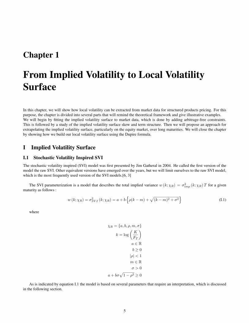
I.1 Stochastic Volatility Inspired SVIThe stochastic volatility inspired (SVI) model was first presented by Jim Gatheral in 2004. He called the first version of themodel the raw SVI. Other equivalent versions have emerged over the years, but we will limit ourselves to the raw SVI model,which is the most frequently used version of the SVI models.[6, 3]

The SVI parameterization is a model that describes the total implied variance w (k;χR) = σ2imp (k;χR)T for a given

maturity as follows :

w (k;χR) = σ2SV I (k;χR) = a+ b

{ρ(k −m) +

√(k −m)2 + σ2

}(I.1)

where

χR = {a, b, ρ,m, σ}

k = log

(K

FT

)a ∈ Rb ≥ 0

|ρ| < 1

m ∈ Rσ > 0

a+ bσ√

1− ρ2 ≥ 0

As is indicated by equation I.1 the model is based on several parameters that require an interpretation, which is discussedin the following section.

5

I.1.1 Parameters interpretation

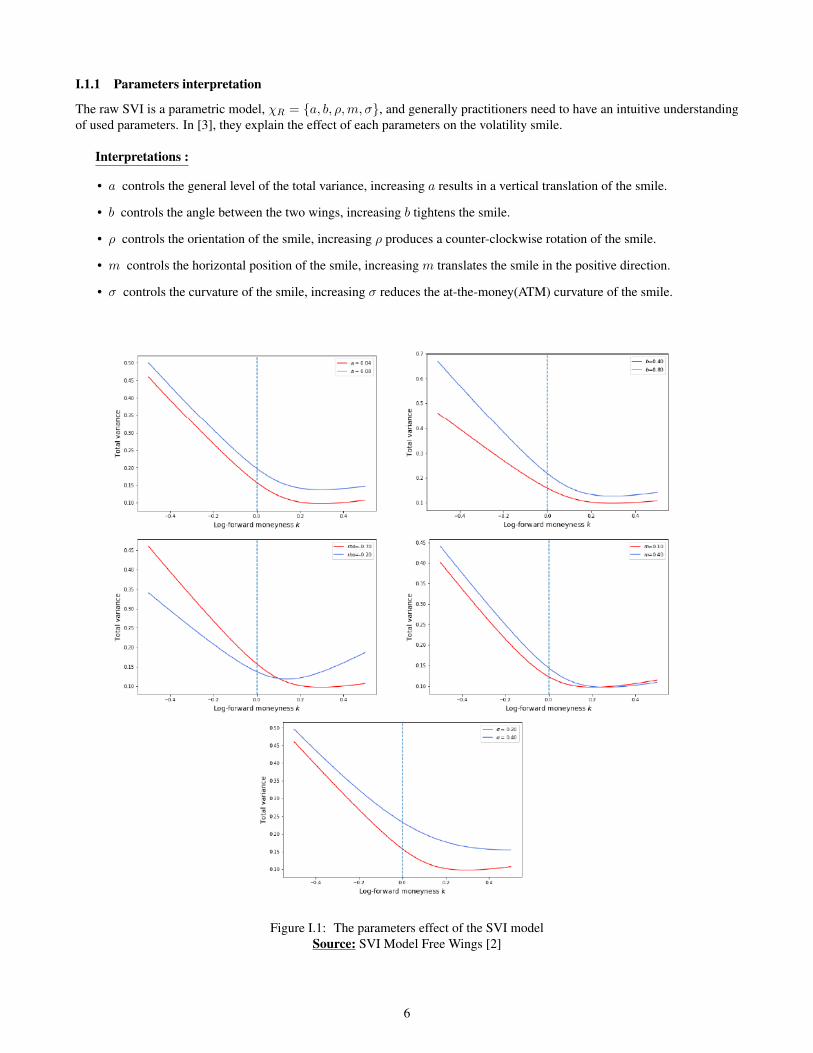
The raw SVI is a parametric model, χR = {a, b, ρ,m, σ}, and generally practitioners need to have an intuitive understandingof used parameters. In [3], they explain the effect of each parameters on the volatility smile.

Interpretations :

• a controls the general level of the total variance, increasing a results in a vertical translation of the smile.

• b controls the angle between the two wings, increasing b tightens the smile.

• ρ controls the orientation of the smile, increasing ρ produces a counter-clockwise rotation of the smile.

• m controls the horizontal position of the smile, increasing m translates the smile in the positive direction.

• σ controls the curvature of the smile, increasing σ reduces the at-the-money(ATM) curvature of the smile.

Figure I.1: The parameters effect of the SVI modelSource: SVI Model Free Wings [2]

6

I.1.2 Model Properties

The SVI model has some properties/strengths that led to its popularity:

• For a fixed maturity T, and large or small strike, the implied total variance wSV Iimp (k;T ) is linear, with respect to the logforward moneyness strike k = log (K/FT ) as |k| → ∞. This result is consistent with Roger Lee’s moment formula[8].

• In [5], Gatheral and Jacquier, showed that in the long maturities, the implied volatility in the Heston model is exactlySVI.

• One can easily calibrate the model in order to avoid calendar spread arbitrage.

I.2 Arbitrage-Free ConditionsIn order to ensure that our volatility is free of arbitrage, two conditions need to be satisfied :

1. For each maturity, there should be no butterfly arbitrage.

2. The surface should be free of calendar spread arbitrage.

I.2.1 Calendar Spread Arbitrage

A calendar spread typically involves buying and selling the same type of option for the same underlying at the same strike, butat different expiration dates. Calendar spread arbitrage is assimilated to the monotonicity of European Call option prices withrespect to the maturity. Knowing that our work mainly focuses on volatility surface, we will try to give an equivalent conditionin order to ensure an implied volatility parameterization to be free of calendar spread arbitrage. For the sake of simplicity, wewill consider the case where dividends are proportional to the stock price. But a generalization can be found in [3].

Lemma I.1. The volatility surface w is free of calendar spread arbitrage if and only if :

∂Tw(k, T ) ≥ 0, for all k ∈ R and T > 0 (I.2)

Graphically : We can interpret the absence of calendar spread by the fact that there are no cross lines on the total variancewhen the maturity goes up, the SVI slice will be translated up.

I.2.2 Butterfly Arbitrage

Butterfly spread consists of using four option contracts with the same maturity T but with three different (equidistant) strikeprices : a higher strike price (K+ ε), an at-the-money strike price (K), and a lower strike price (K− ε). The options with thehigher and lower strike prices are the same distance from the at-the-money options. The strategy consists in buying one calloption with strike K − ε and one call option with strike K + ε and selling two call options on the same strike K. The price ofthe strategy is :

C(K − ε, T )− 2C(K,T ) + C(K + ε, T ) (I.3)

We can notice that this corresponds to the numerator of the second derivative of a call price with respect to the strike K :

d2C(K,T )

dK2

Thus, ensuring butterfly-free arbitrage is equivalent to the condition for the call price convexity. Now, let’s find an equivalencefor the SVI model.

7

Definition I.1.Let’s rewrite the Black-Scholes formula in terms of total implied variance,

CBS(k,w(k)) = S(N (d+(k))− ekN (d−(k))

), for all k ∈ R (I.4)

with N as the Gaussian cdf and d±(k) := −k/√w(k) ±

√w(k)/2 By deriving twice the BS formula, the result should be

equal to density function of the underlying stock

p(k) =∂2CBS(k,w(k))

∂K2

∣∣∣∣K=Ftek

=g(k)√2πw(k)

exp

(−d−(k)2

2

), for any k ∈ R (I.5)

The function g : R→ R

g(k) :=

(1− kw′(k)

2w(k)

)2

− w′(k)2

4

(1

w(k)+

1

4

)+w′′(k)

2

A slice is said to be free of buttery arbitrage if the corresponding density is non-negative, which is equivalent to g(k) ≥ 0.

Lemma I.2. A slice is free of butterfly arbitrage if and only if g(k) ≥ 0 for all k ∈ R and limk→+∞ d+(k) = −∞

I.3 Problem Formulation - Calibration(s)In this section, we will explain how to integrate the arbitrage constraints, set boundaries for all parameters and give theoptimization problem that need to be implemented so as to calibrate the SVI Model. This section was mainly inspired by thework of Tahar Ferhati [2].

I.3.1 Calendar Spread Arbitrage

In order to avoid calendar arbitrage, we need to first impose T0 that ∀k ∈ R, w(k, T0) > 0 for the closest maturity. Then forTi, we have to impose the lower barrier for each k by using the previous maturity parameters. w (k, T0) > 0

w (k, Ti) > w (k, Ti−1) 1 ≤ i ≤ n(I.6)

I.3.2 Butterfly Arbitrage

Axel Vogt [4] proposed an example of parameterization that allows butterfly arbitrage for extreme strikes (particularly on theright wings of our density function g(k)) and that ensures that both of the wings are positive. This example also makes surethat ensuring the positive nature of the minimum implied total variance is sufficient to guarantee butterfly-free arbitrage.

Let’s recall that Roger Lee proved that the left and right wings of the total implied variance are linear with respect to thelog forward-moneyness k.

Theorem I.3 (Butterfly arbitrage-free Constraints). For a given maturity, the total implied variance generated by the SVImodel is free of butterfly arbitrage if the following constraints are verified by its parameters χR:

(a−mb(ρ+ 1))(4− a+mb(ρ+ 1))

b2(ρ+ 1)2> 1

(a−mb(ρ− 1))(4− a+mb(ρ− 1))

b2(ρ− 1)2> 1

0 < b2(ρ+ 1)2 < 4

0 < b2(ρ− 1)2 < 4

(I.7)

8

I.3.3 Optimization Problem

From all this information, we will define an optimization problem for the SVI calibration.

Given a dataset of Total Implied Variance ωmarketki = Tσ2

implied(ki, T ), our objective function for a given maturity T and aset of strike (Ki)1≤i≤n will be :

f (ki;χR) =∑ni=1

[a+ b

{ρ(ki −m) +

√(ki −m)2 + σ2

}− ωmarket

ki

]2, With ki := log

(KiFT

)(I.8)

Two hard constraint functions g1 (χR) and g2(ki;χ

TR;χT−1R

)that will implement respectively theorem I.3 and equation

I.6.We will add some more constraints, regarding parameters Boundaries from C. Martini and S. De Marco work [10].

χR ∈ R5, (χR)l ≤ χR ≤ (χR)u

In summary,

minχR∈R5 f (ki;χR)

subject to:

g1 (χR) ≥ 0 for each ki

g2(ki;χ

TR;χT−1R

)≥ 0 for each ki

(χR)l ≤ χR ≤ (χR)u

(I.9)

In order to solve this non-linear problem, we will use the Sequential Least-Squares Quadratic Programming(SLSQP)algorithm. For the sake of accuracy, we only calibrate the SVI model, for a given maturity, only if we have 5 market data.

II Skew and Term StructureOn the volatility surface, when we fix the maturity and look at the implied volatilities through strikes, we obtain what is knownas the implied volatility smile or skew. Fixing a strike and looking at the implied volatility, we see what is known as the termstructure of volatilities.

II.1 SkewIn equity markets, the implied volatility plot is distorted on one side, which means options with low strikes have higherimplied volatilities than those with higher strikes. In this market, investors need to protect against decreases of value ratherthan increases of value of the stock (covering the downside risk). In this sense, the skew can be seen as the concept ofinsurance. By no-arbitrage arguments, it seems clear that, due to supply and demand reasons, volatilities will be higher atcertain strikes. In practice, big jumps in spot tend to be downward rather than upward. The skew is also used to refer to theslope of the implied volatility as defined by the following equation :

Skew =dσImplied (K)

dK(II.1)

In practice, for measuring the skew, we take the difference between the implied volatility at strikes of 95% and 105% ofthe forward price (others use 90%− 110% or θputdelta25% − θcalldelta25%).

Skew = σ95% − σ105% (II.2)

Generally, the skew is steeper for short-term maturities than for long-term maturities as the time value of the ATM optionis far less sensitive to volatility on short-term maturity.

9

II.2 The Smile CurvatureWhen looking at the smile, we can notice that implied volatility tends "to flatten" out with respect to strikes. Nevertheless, itgrows rapidly as the strikes decrease. For deep Out-Of-the-Money option (put or call), the price extracted from the screen isnever zero. This is explained by the fact that market makers never sell an option at zero (usually min = 0.01 USD). Therefore,the smile is in part due to supply-and-demand, as inverting Black-Scholes or inverting Binomial trees process from the optionprice to get the implied volatility will lead to very high volatilities on the wings, especially far away from the spot level.

The Skew’s convexity help to measure the curvature of the smile :

Convexity =d2σimplied (K)

dK2(II.3)

In practice, to measure the skew one can consider the sum of the 95% and the 105% implied volatility minus twice the100% strikes divided by 2. This is expressed as follows :

Convexity =σ95% + σ105% − 2σ100%

2(II.4)

Smile curvature tends to decrease as maturities increase.

II.3 Term StructureBy seeing term structures of implied volatilities, traders can improve assumption for whether an option with short-term matu-rities will rise or fall later on. In the event that the term structure is rising, where the implied volatilities of long-term optionsare higher than that of short-term maturities, the short-term implied volatility is expected to rise. In the event that the impliedvolatility of short-term maturities is lower than those for long-term maturities, short-term volatility is required to fall.

II.4 Stylized FactsIn [11], they demonstrated that the functions Skew(T ), Convexity(T ) and TermStructure(T ) follow some power law overtime.

Skew(T ) ∼ 1

Tα

Convexity(T ) ∼ 1

T β

TermStructure(T ) ∼ 1

T γ

10

III Implied Volatility for Long-Term MaturitiesFor some structured products, practitioners need to price them over very long-term maturities. Hence, they have to estimate theimplied volatilities for those maturities. Generally, it is very difficult to find an estimation of the long-term implied volatilitieson data providers system such as Bloomberg and the like.

To handle this, we will consider the fact that skew, convexity and term structure follow some power law and that bydetecting the exponent of each law (α ,β , γ) using the short-term implied volatilities data we are able to approximate themeasure of these metrics at any point in time. For any given maturity T , this will lead to the following system of equation :

σ95% − σ105% = 1Tα

σ95%+σ105%−2σ100%

2 = 1Tβ

σ100% = 1Tγ

(III.1)

or σ95% = 1

2 ∗ ( 1Tα + 2

Tβ+ 2

Tγ )

σ105% = 12 ∗ (− 1

Tα + 2Tβ

+ 2Tγ )

σ100% = 1Tγ

(III.2)

Doing the same procedure with 90% − 110%, instead of 95% − 105% allows to generate 5 implied volatility points(σ90%, σ95%, σ100%, σ105% and σ110%) for any given maturity.

From the 5 points of implied volatility generated, particularly for long-term maturities, we can re-run our SVI Model withthe arbitrage constraints in order to build the complete surface over long-term maturity.

IV Local VolatilityLocal Volatility is the instantaneous volatility of an underlying at any given local point. It helps to explain why pricing withthe Black- Scholes formula gives different prices for different strikes and maturities.

Bruno Dupire, Emanuel Derman and Iraj Kani thought of local volatilities as representing some kind of average over allpossible instantaneous volatilities in an effective theory.

In this section, we will show the procedure for obtaining the local volatility surface from the implied volatility surface.It is worth noting that local volatility surface is very sensitive to any discrepancy in the implied volatility surface, especiallyin case of jumps, leading to an extreme level of local volatility. Therefore, before converting the implied volatility into localvolatility, we have to ensure the following two points :

- no arbitrage (calendar and butterfly)

- implied volatility smoothness

IV.1 Derivation of the Dupire EquationLet’s consider the stochastic differential equation representing the asset price process, assumed under the risk neutral proba-bility measure Q :

dStSt

= (rt − qt) dt+ σ (t, St) dWt (IV.1)

where the volatility is now a deterministic function of time and the asset prices, rt and qt, represent respectively the risk-freerate and repo rate.

Let’s define the density distribution of the asset price at maturity as P (T, ST ).Then the Fokker-Planck equation will be :

∂P (t, St)

∂t= − (rt − qt)

∂

∂S[StP (t, St)] +

1

2

∂2

∂S2

[σ(t, St)

2S2t P (t, St)

](IV.2)

11

The discount rate B0,T from the current time t to maturity T is :

B0,T = e−∫ T0rsds (IV.3)

C(K,T ) is the price of an call option with strike K and maturity T .

C(K,T ) = B0,T

∫ ∞0

(s−K)+ P (T, s) ds (IV.4)

By deriving the call price formula with respect to K, we get :

σ(T,K)2 = 2∂C∂T + (rT − qT )K ∂C

∂K + qTC

K2 ∂2C∂K2

(IV.5)

IV.2 Local Volatility in terms of Implied VolatilityBy expressing the Black-Scholes formula in terms of total implied variance, w, we can deduce an expression of the localvolatility in terms of implied volatility. We will give here a short description of the proof. In his book [3], Gatheral provides amore detailed proof.

When using the Black-Scholes model, market prices of options are priced with the implied volatility σBS (K,T : S0).Then,

C (S0,K, T ) = CBS (S0,K, σBS (S0,K, T ) , T ) (IV.6)

For more convenience, we will express the Black-Scholes closed formula in terms of the total implied variance w defined by :

w (S0,K, T ) := σBS2 (S0,K, T )T

and the log-Forward moneyness k defined by

k = log

(K

FT

)In terms of these variables, the Black-Scholes formula becomes :

CBS (FT , k, w) = FT[N (d1)− e2N (d2) |

= FT

{N

(− k√

w+

√w

2

)− ekN

(− k√

w−√w

2

)}We will now calculate all the partial derivatives needed and then plug them into the Dupire Formula.

∂C

∂K=∂C

∂k

∂k

∂K+∂C

∂w

∂w

∂K∂C

∂K=

1

K

∂C

∂k+∂w

∂K

∂C

∂w

(IV.7)

Replacing these partial derivatives in the Dupire Formula demonstrated above and simplifying it give an expression of thelocal volatility in terms of the total implied variance, w, and the log-forward moneyness k, expressed as follows :

σ2L =

∂w∂T + (rT − qT )K ∂w

∂K

1 +K ∂w∂K

(12 −

kw

)+ 1

2K2 ∂2w∂K2 − 1

4K2(∂w∂K

)2 ( 14 + 1

w −k2

w2

) (IV.8)

12

V Numerical ResultsFor the sake of completeness, we built our volatility surface for strikes between 0 and 3×spot.

V.1 Calendar arbitrageAfter calibration, we plotted the total implied variance for different maturities. We also looked at the total implied variancesurface as a function of the maturities T and log-forward moneyness k. We noticed that for a given k the total implied varianceis monotonically increasing, which implies that we succeeded to avoid calendar arbitrage in our interpolation.

Figure V.1: Total implied variance as a function of the log-forward moneyness, for different maturities

(a) (b)

Figure V.2: Total Variance surface

13

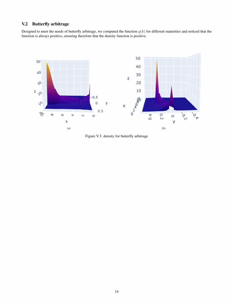
V.2 Butterfly arbitrageDesigned to meet the needs of butterfly arbitrage, we computed the function g(k) for different maturities and noticed that thefunction is always positive, ensuring therefore that the density function is positive.

(a) (b)

Figure V.3: density for butterfly arbitrage

14

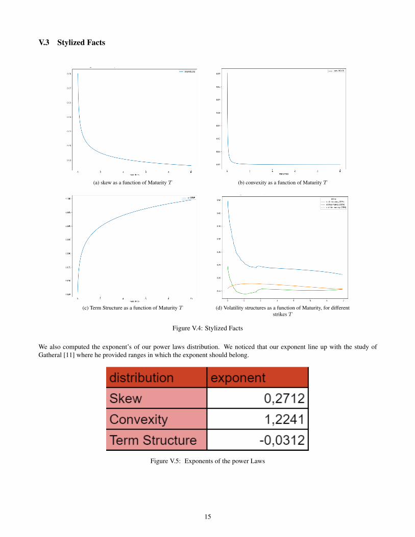
V.3 Stylized Facts

(a) skew as a function of Maturity T (b) convexity as a function of Maturity T

(c) Term Structure as a function of Maturity T (d) Volatility structures as a function of Maturity, for differentstrikes T

Figure V.4: Stylized Facts

We also computed the exponent’s of our power laws distribution. We noticed that our exponent line up with the study ofGatheral [11] where he provided ranges in which the exponent should belong.

Figure V.5: Exponents of the power Laws

15

V.4 error of estimationsGeared toward interpolating the implied volatility data from Bloomberg, we needed to check if our results was aligned withthe initial data. To check that, we decided to calculate the root mean squared error (RMSE) between the implied volatilityfrom bloomberg and the implied volatility resulting from the SVI Model for different maturities.

Figure V.6: RMSE of the Implied Volatility for different Maturities

16

V.5 Local and Implied Volatility Surface

(a) views from maturities side (b) views from strikes side

Figure V.7: Implied Volatility surface

(a) (b)

Figure V.8: Local Volatility surface

17

Chapter 2

Monte-Carlo Simulations and Model

In this chapter, we will present and discuss the different steps adopted in order to estimate the price of our underlyings.The chapter is organized in four sections. We will begin with a brief discussion of the Monte-Carlo principle, then we willintroduce the stochastic differential equations that are used in this study. The following section explains our approach tocorrelated assets simulation. Finally, we will discuss the results we obtained in the last part.

I Monte-Carlo PrincipleThe price of an asset can be calculated by simulating N independent trajectories

(S1t

)0<t<T

, . . . ,(SNt)0<t<T

. For each ofthese trajectories, we calculate g

(Sit , 0 ≤ t ≤ T

), the amount of the corresponding discounted future flows. The strong law

of large numbers ensures the convergence of the arithmetic mean of the simulated values towards the price.Monte Carlo simulation techniques use the strong law of large numbers to estimate the desired value Vg . If the curves

(Si)1≤i≤N ={Sit , 0 ≤ t ≤ T

}represent N independent trajectories distributed according to the same law, then IN , which is

an estimator of the underlying price, converges to Vg .

IN =1

N

N∑i=1

g(Si) p.s.→ Vg (I.1)

The central limit theorem gives an idea of the approximation achieved. And given the fact that the second order momentof g (St, 0 ≤ t ≤ T ) is finite, we have :

√N

(1

N

N∑i=1

g(Si)− Vg

)loi→ N (0,Var[g(S)]) (I.2)

We can notice that the higher the variance V ar[g(S)], the more simulations (N) are needed to obtain an accurate estimatorIN . Practically, it can be computationally expensive to raise the number of paths generated. That’s why practitioners tend touse alternative approaches by controlling the variance of g V ar[g(S)]. However, this technique, called the variance reductiontechnique, will not be discussed in this work.

18

II Local Volatility Model and Mono-Asset Diffusion

II.1 Local Volatility ModelIn the local volatility model, volatility is assumed to be a deterministic function of asset price and time. It was created afterDupire demonstrated that consistent models can be constructed in the presence of volatility skews if the asset price SDE isassumed to have the following dynamics under the risk neutral probability measure Q.

dStSt

= (rt − qt) dt+ σ (t, St) dWt (II.1)

where,

rt, the risk-free interest rate (deterministic)

qt, the repo-rate (deterministic)

σ (t, St), the volatility as a deterministic function of time and the asset price

Wt, the standard brownian motion

The only stochastic behavior (one factor model) implemented into the volatility equation in the local volatility model isdue to it being a function of the underlying asset price. As a result, there is only one source of stochasticity, guaranteeing theBlack-Scholes model’s completeness. Completeness is critical because it ensures that prices are unique.

II.2 DiscretizationIn order to solve the SDE, we will use the the log-Euler scheme. This allows us to preserve the positivity of the asset price.Let’s suppose that our stock price follows a local volatility model and define Yt = ln (St). Applying Itˆo’s lemma gives :

dYt =(rt − qt − 0.5σ (t, Yt)

2)dt+ σ (t, Yt) dWt (II.2)

then the local volatility function being piecewise constant, we obtain after discretization :

∆Y (ti) ≈(r (ti)− q (ti)− 0.5σ (ti, Yti)

2)

∆ti + σ (ti, Yti) ∆Wti (II.3)

Finally,

S (ti+1) ≈ S (ti) exp[(r (ti)− q (ti)− 0.5σ (ti, Sti)

2)

∆ti + σ (ti, Sti) ∆Wti

](II.4)

with, r(ti) and q(ti), respectively, instantaneous risk-free rate and repo rate.As a basis, we use 365 days per year time frame, with 5 business days per week but we only use our diffusion on business

days.

II.3 Discrete DividendThe majority of stocks do pay dividends. Taking into account the dividend Dti paid at a given time ti will produce a jump ofDti in the present value of the stock at time ti, then a discontinuity in our stock price.

In our diffusion scheme we adjust the asset price for all days when dividends are paid (Equation II.5).

S̃ti = Sti −Dti (II.5)

where Dti is the dividend paid at time ti .

19

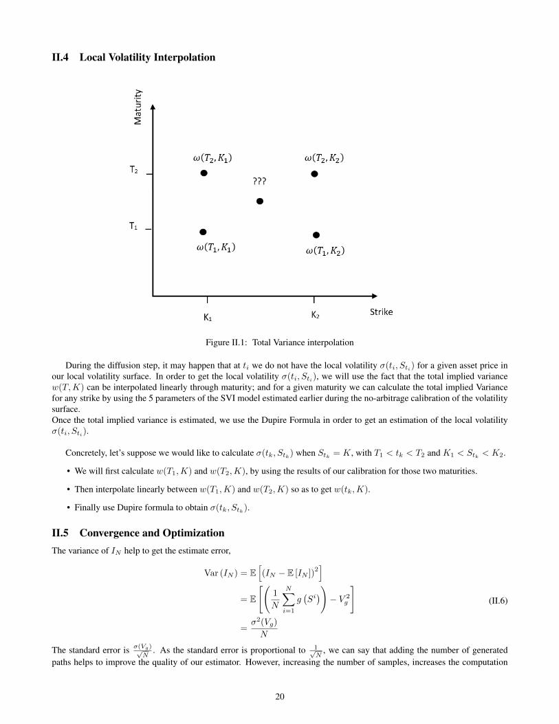
II.4 Local Volatility Interpolation

Figure II.1: Total Variance interpolation

During the diffusion step, it may happen that at ti we do not have the local volatility σ(ti, Sti) for a given asset price inour local volatility surface. In order to get the local volatility σ(ti, Sti), we will use the fact that the total implied variancew(T,K) can be interpolated linearly through maturity; and for a given maturity we can calculate the total implied Variancefor any strike by using the 5 parameters of the SVI model estimated earlier during the no-arbitrage calibration of the volatilitysurface.Once the total implied variance is estimated, we use the Dupire Formula in order to get an estimation of the local volatilityσ(ti, Sti).

Concretely, let’s suppose we would like to calculate σ(tk, Stk) when Stk = K, with T1 < tk < T2 and K1 < Stk < K2.

• We will first calculate w(T1,K) and w(T2,K), by using the results of our calibration for those two maturities.

• Then interpolate linearly between w(T1,K) and w(T2,K) so as to get w(tk,K).

• Finally use Dupire formula to obtain σ(tk, Stk).

II.5 Convergence and OptimizationThe variance of IN help to get the estimate error,

Var (IN ) = E[(IN − E [IN ])

2]

= E

[(1

N

N∑i=1

g(Si))− V 2

g

]

=σ2(Vg)

N

(II.6)

The standard error is σ(Vg)√N

. As the standard error is proportional to 1√N

, we can say that adding the number of generatedpaths helps to improve the quality of our estimator. However, increasing the number of samples, increases the computation

20

time, which might be expensive. There are alternative approaches to improve efficiency of our estimator/computation timesuch as :

• variance reduction techniques

• reducing the number of observation date by choosing a constant step of 1 observation/week instead of 1 observation/day

• Changing the way we generate our random Walk at the first step of our Monte-Carlo simulation

This last method is called quasi Monte-Carlo, in contrast to a classical Monte-Carlo, where we use pseudo-random se-quence numbers. With the quasi Monte-Carlo, we generate a low-discrepancy sequence (the sampling points are equallydistributed over space), which helps to avoid the clustering illusion that may rise from random sampling, but also helps toreduce the standard deviation. The latter results in improving the convergence speed of our simulation. These changes leadus to modify our discretization scheme in order to take into account informations( dividends, rates variation,...) betweenobservations dates.We took as final scheme,

S̃ (ti+1) = S̃ (ti) exp

{∆t

6∑k=0

[(r (ti + k)− q (ti + k))]

}× exp

{−0.5σ (ti, Sti)

27∆t+ σ (ti, Sti) (Wti+1

−Wti)}

-∑6l=1Dti+l exp

{∆t∑6k=i [(r (ti + k)− q (ti + k))]

}−Dti+1

(II.7)By taking a closer look to this formula, one can notice that we capitalized all the dividends between two observation dates

to the forthcoming observation date. To do so, we needed to convert our actuarial rates to forward exponential rates. That isrealized using the following formula :

rti+k,ti+1 = exp

{rti+1

ti+1 − rti+k(ti + k)

ti+1 − (ti + k)

}− 1 (II.8)

The same reasoning applies to the repo-rate. We also added a spot modulator factor to our initial dividend at each step asexpressed in the following equation :

Dti+l = Dti+lStiFti

∀l ∈ [1, 7] (II.9)

In other words, the higher the spot, the higher the dividend, and vice-versa.

III Multi-dimensional SimulationPractitioners and scholars alike often use multi-dimensional models. Many financial institutions, as well as academic institu-tions, use derivatives on several state variables, such as multi-asset options (i.e. basket options).

Since analytic formula to such problems are only available in a few specific cases, numerical methods such as Monte-Carlo are extremely useful, particularly when considering the interdependence of the various factors (or underlying assets).Therefore, the question of how to specify a correlation matrix arises in a number of key areas of finance.

For high-dimensional models with correlation, the Monte-Carlo method is relatively simple. For models that need morethan one stochastic factor, we will show how to generate correlated stochastic processes in terms of standard Brownianmotions.

It is possible to simplify the problem of generating correlated stochastic processes by generating correlated random vari-ables. We decided to use constant correlations so as not to complexify our model.

Now, let’s suppose we have D assets (Si)1≤i≤D whose prices are driven by a Local volatility model, dW (t), a D -dimensional Brownian motions vector (independent)

dW (t) =

dW1(t)...

dWD(t)

21

and a correlation matrix C,which must be a positive semi-definite matrix

C =

c11 c12 · · · c1D

c21 c12 · · · c1D...

.... . .

...

cD1 cD2 · · · cDD

(III.1)

As C is a positive semi-definite matrix, then there exist a lower triangular matrix L so that :

LL> = C (III.2)

To extract L, we used Cholesky factorisation method.Once obtained, the Lower Triangular Matrix can be used in order to have the desired correlated Brownian motions,

dW̃ (t) =

dW̃1(t)...

dW̃D(t)

= L

dW1(t)...

dWD(t)

(III.3)

Expressed in a matrix-like form, the different dynamics of our assets are :

dS1(t)...

dSD(t)

= diag(S1(t) , · · · , SD(t))

drift1(t)...

driftD(t)

dt+ diag(σ1(t) , · · · , σD(t))dW̃ (t)

(III.4)

with

• diag(σ1(t) , · · · , σD(t)) a D ×D diagonal matrix with σi(t) the local volatility of the asset i at time t

• drifti(t) = ri(t)− qi(t) the risk-free interest rate minus the repo rate of the asset i at time t

IV Numerical ResultsIn order to check out the result of our diffusion, we had realized different test that are presented in the following subsections.

IV.1 Correlation Multi-AssetsLet’s generate 3 sequences of random walk (Bt,Wt, Zt) and check if they are completely decorrelated. After calculating theircorrelation matrix we get :

1 −0.001 0.001

−0.001 1 0

0.001 0 1

(IV.1)

After verification, we can say that our random walks are almost decorrelated. Now, let’s define C as the correlation matrixthat we would like to have between our different assets as follows :

C =

1 0.2 0.4

0.2 1 0.5

0.4 0.5 1

(IV.2)

Now, when we apply Cholesky decomposition so as to find our lower triangular matrix and see if (B̃t, W̃t, Z̃t) have thecorrelation desired, we have the following results :

22

L =

1 0 0

0.2 0.9797959 0

0.4 0.4286607 0.81009259

(IV.3)

Corr(B̃t, W̃t, Z̃t) =

1 0.20100322 0.39949249

0.20100322 1 0.50032208

0.39949249 0.50032208 1

(IV.4)

Considered as equal, we will verify the correlations of our diffused assets, which is :

Corr(S̃1, S̃2, S̃3) =

1 0.10570807 0.33267551

0.10570807 1 0.39488099

0.33267551 0.39488099 1

(IV.5)

We noticed that the correlation slightly changed. This change can be explained by drift terms and dividends.

IV.2 Convergence of the Empirical mean of the stock Price to the Forward PriceWe had also tested if, at a given time, the forward price converged to the mean of all the trajectories. As the forward contractscan also be a way to lock in pricing, for a given maturity.For the sake of precision, we defined an interval of confidence H , with α = 95%.

H =

[E(Si)− q1−α2

σ(Si)√N

,E(Si) + q1−α2σ(Si)√N

](IV.6)

with N , the number of trajectories generated.

23

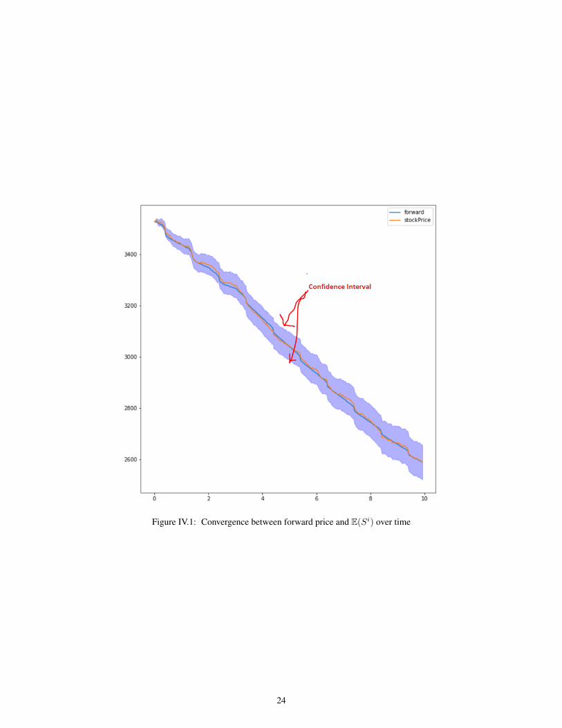
Figure IV.1: Convergence between forward price and E(Si) over time

24

Chapter 3

Structured Products

In this chapter, we will present our process for getting the fair coupon rate when offering structured products.First, we will present an overview on structured products. Then, we will talk about some products used in our study as wellas our approach to get the fair coupon rate. We end the chapter with a comparison between the output of our model and theoffers proposed by some issuers in the market.

I Overview on structured productsA combination of vanilla options allowed banks to offer more sophisticated products such as structured products that suit moreinvestor necessities. A structured note is composed of :

• a non risky asset, which represents a part of the protected capital. Generally, it can be a zero coupon bond that will paya sealed amount or a bond that will pay the principal plus the initially agreed interest.

• a risky asset, which represents a leverage potential that can be an option on a single or multiple assets. The latter issubject to many market parameters that can enable holders to make great profit, but also that can make them loose theirentire value.

Figure I.1: Composition of structured noteSource: Exotic Options and Hybrids – A Guide to Structuring, Pricing and Trading

Autocallables are structured products, commonly traded exotics options. Also called auto-trigger structures, they getcalled when the underlying breaches a barrier, in general the maturity of the trade vary depending on the performance of theunderlying at the pre-fixed observation dates prior to the expiration date. There are many variations in terms of structures forautocallables products.

In the following, we will try to define general features for these types of products and present some of them that we willuse later on.

Let’s define:

25

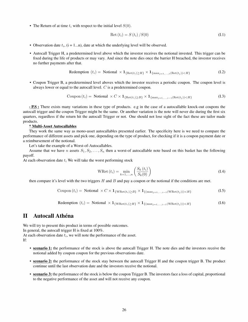
• The Return of at time ti with respect to the initial level S(0).

Ret (ti) = S (ti) /S(0) (I.1)

• Observation date ti, (i = 1...n), date at which the underlying level will be observed.

• Autocall Trigger H, a predetermined level above which the investor receives the notional invested. This trigger can befixed during the life of products or may vary. And since the note dies once the barrier H breached, the investor receivesno further payments after that.

Redemption (ti) = Notional × 1{Ret(ti)≥H} × 1{maxj=1,...,1(Ret(tj))<H} (I.2)

• Coupon Trigger B, a predetermined level aboves which the investor receives a periodic coupon. The coupon level isalways lower or equal to the autocall level. C is a predetermined coupon.

Coupon (ti) = Notional × C × 1{Ret(ti)≥B} × 1{maxj=1,...,i−1(Ret(tj))<H} (I.3)

- P.S : There exists many variations in these type of products. e.g in the case of a autocallable knock-out coupons theautocall trigger and the coupon Trigger might be the same. Or another variation is the note will never die during the first sixquarters, regardless if the return hit the autocall Trigger or not. One should not lose sight of the fact these are tailor madeproducts.

* Multi-Asset AutocallablesThey work the same way as mono-asset autocallables presented earlier. The specificity here is we need to compare the

performance of different assets and pick one, depending on the type of product, for checking if it is a coupon payment date ora reimbursement of the notional.

Let’s take the example of a Worst-of-Autocallables.Assume that we have n assets S1, S2, . . . , Sn then a worst-of autocallable note based on this basket has the following

payoff.At each observation date ti We will take the worst performing stock

WRet (ti) = mink=1,...,n

(Sk (ti)

Sk(0)

)(I.4)

then compare it’s level with the two triggers H and B and pay a coupon or the notional if the conditions are met.

Coupon (ti) = Notional × C × 1{WRet(ti)≥B} × 1{(maxj=1,...,i−1(WRet(tj)))<H} (I.5)

Redemption (ti) = Notional × 1{WRet(ti)≥H} × 1{(maxj=1,...,i−1(WRet(tj)))<H} (I.6)

II Autocall AthénaWe will try to present this product in terms of possible outcomes.In general, the autocall trigger H is fixed at 100%.At each observation date ti, we will note the performance of the asset.If:

• scenario 1: the performance of the stock is above the autocall Trigger H. The note dies and the investors receive thenotional added by coupon coupon for the previous observations date.

• scenario 2: the performance of the stock stay between the autocall Trigger H and the coupon trigger B. The productcontinue until the last observation date and the investors receive the notional.

• scenario 3: the performance of the stock is below the coupon Trigger B. The investors face a loss of capital, proportionalto the negative performance of the asset and will not receive any coupon.

26

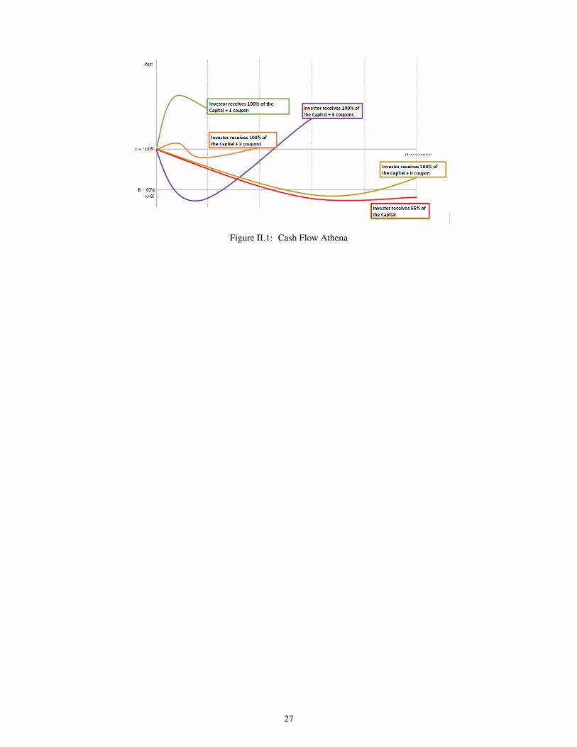
Figure II.1: Cash Flow Athena

27

III Numerical Results

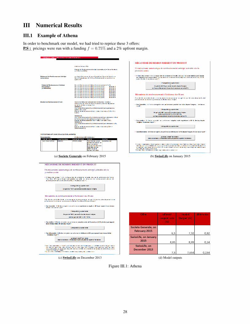
III.1 Example of AthenaIn order to benchmark our model, we had tried to reprice these 3 offers:P.S : pricings were run with a funding f = 0.75% and a 2% upfront margin.

(a) Societe Generale on February 2015 (b) SwissLife on January 2015

(c) SwissLife on December 2013 (d) Model outputs

Figure III.1: Athena

28

III.2 The effect of Correlation on multi-asset optionsIn the following, we put a particular focus on correlation and not dispersion.In order to describe the effects of correlation on multi-asset equity options, we decided to run our multi-asset model withdifferent correlation matrix and observe the variation on price of product like Best-of/Worst-of.

Clow =

1 0.2 0.4

0.2 1 0.5

0.4 0.5 1

and Chigh =

1 0.8 0.9

0.8 1 0.85

0.9 0.85 1

(III.1)

Assume that we have 3 assets S1, S2, S3 then our options have the following payoffs at strike K and maturity T .For a better comparatility, we used the return of the assets instead of the assets price, K = 1 and T = 10

WO Call payoff = max [0,min (S1(T ), S2(T ), S3(T ))−K]

BO Put payoff = max [0,K −max (S1(T ), S2(T ), S3(T ))]

WO Put payoff = max [0,K −min (S1(T ), S2(T ), S3(T ))]

BO Call payoff = max [0,max (S1(T ), S2(T ), S3(T ))−K]

(III.2)

Figure III.2: Price variation w.r.t correlation

We can see that for a worst-of Call, a lower correlation will likely result in a lower payoff. Which makes sense becausewhen correlation is low, there is a smaller chance that the worst performing stock of the basket ends up above the barrier andends up close to the two other assets. Same reasoning for Best-of Put.

IV sensitivities and Hedging tools

IV.1 sensitivitiesIn the upcoming development, we explain – on a straightforward basis - sensitivities on mono assets, as we already discussedhere above the particularity of correlation levels for multi assets pricing.Structured products can be decomposed as (view of the buyer of an Autocall):

• Long a strips of memory conditional call digitals strike ATM, with pay-off = coupo

• Short a down-and-in put European barrier with strike ATM and barrier level at usually 50% or 60%, maturity withmemory effect.

• Weighting a default risk of the issuer.

29

IV.1.1 Dividend yield

Structured products as a whole are often written on underlyings exhibiting high dividend yield. Therefore, the first parameterwe will challenge is dividends.The first thing to check when you trade structured product is to compare dividend yield of the underlying to the conditionalcoupon you expect to get.Never forget that structured products consist in recycling dividends:The customer sells its dividends – unconditional - to the bank (market maker) which provides him coupon depending on sce-narii.The higher the initial dividend yield of the underlying, the higher the expected coupon.

IV.1.2 Implied volatility and skew

Usually, structured products are marketed as a way to protect investment – until a given downside level – but the marketingargumentation omits the positive outcome.The aim is to compare holding the structured product to holding the underlying.Let’s take the negative outcome first:

• Underlying: temporary negative performance + dividend

• Structured product: nothing until next observation date or maturity

Let’s take the positive outcome:

• Underlying: positive performance + dividend

• Structured product: nothing + coupon

Thus, speaking about implied probability distribution, when buying a structured product, the investor “sells” to the issuerthe right part of the curve (standing for positive future returns), and buys protection on a part of the left side of the curve.

IV.1.3 Issuer rating and default risk (funding risk)

For a given structure (underlying, characteristics. . . ), the coupon level can vary only due to the issuer risk of default. As thestructured product holder bears the risk of seeing the issuer go bankrupt, a weak issuer will exhibit higher coupon levels thana robust issuer.Investors usually forget this parameter when picking up.

30

IV.2 HedgingIV.2.1 Dividend yield

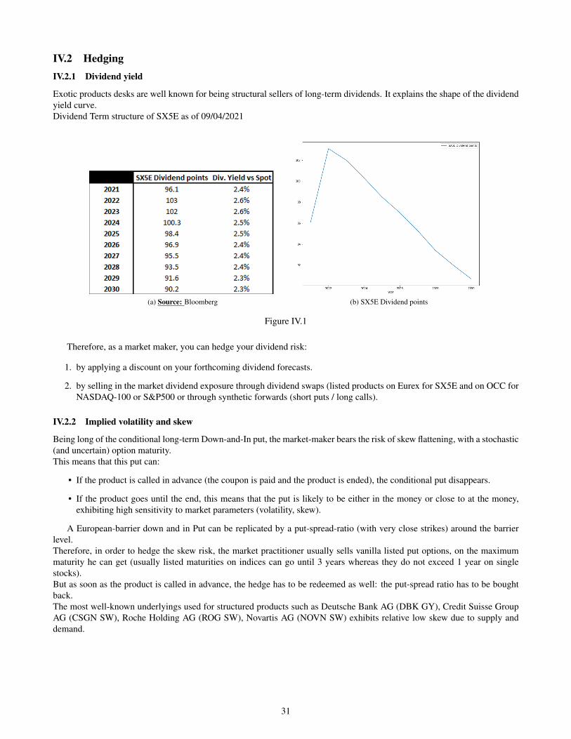
Exotic products desks are well known for being structural sellers of long-term dividends. It explains the shape of the dividendyield curve.Dividend Term structure of SX5E as of 09/04/2021

(a) Source: Bloomberg (b) SX5E Dividend points

Figure IV.1

Therefore, as a market maker, you can hedge your dividend risk:

1. by applying a discount on your forthcoming dividend forecasts.

2. by selling in the market dividend exposure through dividend swaps (listed products on Eurex for SX5E and on OCC forNASDAQ-100 or S&P500 or through synthetic forwards (short puts / long calls).

IV.2.2 Implied volatility and skew

Being long of the conditional long-term Down-and-In put, the market-maker bears the risk of skew flattening, with a stochastic(and uncertain) option maturity.This means that this put can:

• If the product is called in advance (the coupon is paid and the product is ended), the conditional put disappears.

• If the product goes until the end, this means that the put is likely to be either in the money or close to at the money,exhibiting high sensitivity to market parameters (volatility, skew).

A European-barrier down and in Put can be replicated by a put-spread-ratio (with very close strikes) around the barrierlevel.Therefore, in order to hedge the skew risk, the market practitioner usually sells vanilla listed put options, on the maximummaturity he can get (usually listed maturities on indices can go until 3 years whereas they do not exceed 1 year on singlestocks).But as soon as the product is called in advance, the hedge has to be redeemed as well: the put-spread ratio has to be boughtback.The most well-known underlyings used for structured products such as Deutsche Bank AG (DBK GY), Credit Suisse GroupAG (CSGN SW), Roche Holding AG (ROG SW), Novartis AG (NOVN SW) exhibits relative low skew due to supply anddemand.

31

IV.2.3 Correlation

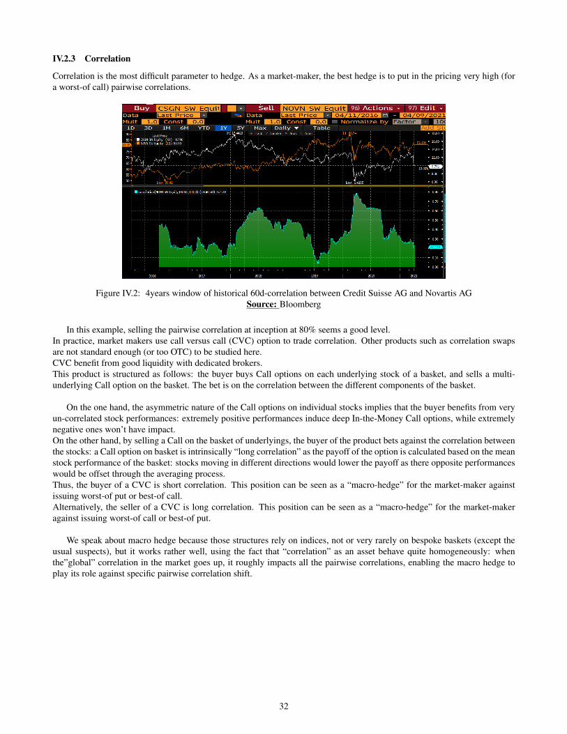
Correlation is the most difficult parameter to hedge. As a market-maker, the best hedge is to put in the pricing very high (fora worst-of call) pairwise correlations.

Figure IV.2: 4years window of historical 60d-correlation between Credit Suisse AG and Novartis AGSource: Bloomberg

In this example, selling the pairwise correlation at inception at 80% seems a good level.In practice, market makers use call versus call (CVC) option to trade correlation. Other products such as correlation swapsare not standard enough (or too OTC) to be studied here.CVC benefit from good liquidity with dedicated brokers.This product is structured as follows: the buyer buys Call options on each underlying stock of a basket, and sells a multi-underlying Call option on the basket. The bet is on the correlation between the different components of the basket.

On the one hand, the asymmetric nature of the Call options on individual stocks implies that the buyer benefits from veryun-correlated stock performances: extremely positive performances induce deep In-the-Money Call options, while extremelynegative ones won’t have impact.On the other hand, by selling a Call on the basket of underlyings, the buyer of the product bets against the correlation betweenthe stocks: a Call option on basket is intrinsically “long correlation” as the payoff of the option is calculated based on the meanstock performance of the basket: stocks moving in different directions would lower the payoff as there opposite performanceswould be offset through the averaging process.Thus, the buyer of a CVC is short correlation. This position can be seen as a “macro-hedge” for the market-maker againstissuing worst-of put or best-of call.Alternatively, the seller of a CVC is long correlation. This position can be seen as a “macro-hedge” for the market-makeragainst issuing worst-of call or best-of put.

We speak about macro hedge because those structures rely on indices, not or very rarely on bespoke baskets (except theusual suspects), but it works rather well, using the fact that “correlation” as an asset behave quite homogeneously: whenthe”global” correlation in the market goes up, it roughly impacts all the pairwise correlations, enabling the macro hedge toplay its role against specific pairwise correlation shift.

32

Conclusion

Throughout this work, pricing of Autocallable structures is addressed using Monte Carlo simulation approach. Choosing themodel for our diffusion was not an easy exercise, as you may notice different structured products may expose to differentfeature sensitivity. The fact that on Equity market, volatility is not the same across strike, lead us to choose a model that takeinto account skew, then a local volatility model. Local volatility models are path-dependant and help to capture the smilewithout not much source of randomness. Calibrating this model, so as to ensure Arbitrage-free, was an interesting exercise.And the results of the model was very satisfying.For further improvement, we will try to implement, alternatively, a stochastic volatility model and a Interest Rate HybridModel With Stochastic Volatility and the Interest Rate Smile for products that need vega convexity and forward skew.

33

Bibliography

[1] Alan Lewis Espen G. Haug, Jørgen Haug. Back to basics: a new approach to the discrete dividend problem. 2003.

[2] Tahar Ferhati. Svi model free wings. 2020.

[3] Jim Gatheral. The volatility surface: A practitionner’s guide. 2006.

[4] Jim Gatheral and Antoine Jacquier. Arbitrage-free svi volatility surfaces. 2014.

[5] Antoine Jacquier Jim Gatheral. A. convergence of heston to svi. 2011.

[6] Antoine Jacquier Jim Gatheral. Arbitrage-free svi volatility surfaces. 2013.

[7] Rui Dilao Joao Amaro de Matos. On the value of european options on a stock paying a discrete dividend.

[8] Roger W. Lee. The moment formula for implied volatility at extreme strikes. volume 14.3, pages 469–480. 2004.

[9] J. W. NIEUWENHUIS M. H. VELLEKOOP. Efficient pricing of derivatives on assets with discrete dividends. 2006.

[10] C. Martini and S. De Marco. Quasi-explicit calibration of gatheral svi model. 2012.

[11] Jim Gatheral Michael Kamal. Implied volatility surfaces. 2010.

[12] M.. Rogers, C. Tehranchi. Can the implied volatility surface move by parallel shift?, 235-248. 2010.

34