frequency-domain system identification for unmanned ... · none of this would have been possible...
TRANSCRIPT

Frequency-Domain System Identification forUnmanned Helicopters from Flight Data
Mohammadhossein Mohajerani
A Thesis
in
The Department
of
Mechanical and Industrial Engineering
Presented in Partial Fulfillment of the Requirements
for the Degree of Master of Applied Science at
Concordia University
Montréal, Québec, Canada
September 2014
c© Mohammadhossein Mohajerani, 2014

CONCORDIA UNIVERSITY
School of Graduate Studies
This is to certify that the thesis proposal prepared
By: Mohammadhossein Mohajerani
Entitled: Frequency-Domain System Identification for Unmanned He-
licopters from Flight Data
and submitted in partial fulfilment of the requirements for the degree of
Master of Applied Science
complies with the regulations of this University and meets the accepted standards
with respect to originality and quality.
Signed by the final examining committee:
Dr. I. Contreras
Dr. W. Zhu , Examiner, External
Dr. B. Gordon, Examiner
Dr. Y. Zhang, Supervisor
Dr. H. Bolandhemmat, Supervisor
Approved byDr. Martin D. Pugh, Chair
Department of Mechanical and Industrial Engineering
Dr. Amir Asif
Dean, Faculty of Engineering and Computer Science

ABSTRACT
Developing accurate and realistic models for Unmanned Aerial Vehicles (UAVs)
is a central task in effective controller design, autopilot design, and simulation model
validation. System identification methods have been extensively used as reliable and
less expensive alternatives for conventional analytical modeling for large-scale aircraft
in the past. Yet, there is limited work on the identification of mathematical models
for small-scale unmanned helicopters. This thesis focuses on development of a system
identification tool for rotary-wing UAVs based on frequency-domain non-parametric
and parametric identification methods. The tool, which is designed to be embedded
in the computer simulation software available for a UAV platform, employs nonlinear
parameter estimation and optimization techniques with the purpose of predicting
dominant dynamics of the UAV from measured responses and controls. The real flight
data acquired from the testbed have been used for testing and verifying the developed
system identification tool. The testbed is a commercially available radio-controlled
helicopter, Trex-700, equipped with MP2128G2Heli MicroPilot autopilot, and the
flight tests are conducted by MicroPilot in hover regime to excite attitude dynamics
of the vehicle. The identification results using the developed tool are validated with
CIFER� framework which is a highly reliable tool in aircraft system identification.
The results demonstrate excellent prediction capability of the developed tool for
model identification of the testing UAV platform.
iii

Dedicated to
My Family
iv

ACKNOWLEDGEMENTS
None of this would have been possible without the love and patience of my
family. My father, my mother, and my sister, to whom this thesis is dedicated, have
been a constant source of love, concern, support and strength all these years. I would
like to express my heart-felt gratitude to my family first.
My deepest gratitude is to my supervisor, Dr. Youmin Zhang. I have been
amazingly fortunate to have a supervisor who gave me the freedom to explore on
my own, and at the same time the guidance to recover when my steps faltered. His
patience and support helped me overcome many crisis situations and finish this thesis.
I am grateful to him for holding me to a high research standard and enforcing strict
validations for each research result. My co-supervisor, Dr. Hamid Bolandhemmat,
has been always there to listen and give advice. I am deeply grateful to him for
the long discussions that helped me sort out the technical details of my work. His
insightful comments and constructive criticisms at different stages of my research
were thought-provoking and they helped me focus my ideas.
I am grateful to my good friend and colleague, Dr. Iman Sadeghzadeh, for his
encouragement and practical advice throughout my studies. I am also thankful to
MicroPilot flight test crew specifically Mr. Nick Playle for performing flight tests on
the helicopter testbed.
Mr. Hossein Babini and Mr. Atabak Sadeghi, my long-time friends and former
classmates, deserve a great appreciation. Their support and care helped me overcome
setbacks and stay focused on my graduate study. Many friends helped me stay sane
through these difficult years. I greatly value their friendship and I deeply appreciate
their belief in me.
v

Finally, I appreciate the financial support from Natural Sciences and Engineer-
ing Research Council of Canada (NSERC) and MicroPilot that funded this research.
vi

TABLE OF CONTENTS
LIST OF FIGURES . . . . . . . . . . . . . . . . . . . . . . . . . . . . . . . . ix
LIST OF TABLES . . . . . . . . . . . . . . . . . . . . . . . . . . . . . . . . . xi
1 Introduction 1
1.1 Research Motivation . . . . . . . . . . . . . . . . . . . . . . . . . . . 5
1.2 Thesis Outline . . . . . . . . . . . . . . . . . . . . . . . . . . . . . . . 7
2 Flight Experiment 8
2.1 Introduction . . . . . . . . . . . . . . . . . . . . . . . . . . . . . . . . 8
2.2 Scope of Input Design . . . . . . . . . . . . . . . . . . . . . . . . . . 10
2.3 Input Detailed Design . . . . . . . . . . . . . . . . . . . . . . . . . . 16
2.3.1 Piloted Frequency Sweep . . . . . . . . . . . . . . . . . . . . . 17
2.3.2 Doublet Input . . . . . . . . . . . . . . . . . . . . . . . . . . . 19
2.4 Introduction to the UAV Testbed . . . . . . . . . . . . . . . . . . . . 22
2.5 Flight Test Implementation . . . . . . . . . . . . . . . . . . . . . . . 23
2.6 Flight Test Results . . . . . . . . . . . . . . . . . . . . . . . . . . . . 26
3 Frequency-Response Identification 28
3.1 Introduction . . . . . . . . . . . . . . . . . . . . . . . . . . . . . . . . 28
3.2 Time-Frequency Transformation . . . . . . . . . . . . . . . . . . . . . 29
3.3 Frequency-Response Function . . . . . . . . . . . . . . . . . . . . . . 31
3.3.1 Rough Estimation of Spectral Quantities . . . . . . . . . . . . 32
3.3.2 Overlapped Windowing . . . . . . . . . . . . . . . . . . . . . . 33
3.3.3 Composite Windowing . . . . . . . . . . . . . . . . . . . . . . 34
3.3.4 Accuracy Metrics . . . . . . . . . . . . . . . . . . . . . . . . . 35
3.4 Identification of the Model . . . . . . . . . . . . . . . . . . . . . . . . 37
3.4.1 Longitudinal Dynamics . . . . . . . . . . . . . . . . . . . . . . 38
vii

3.4.2 Lateral Dynamics . . . . . . . . . . . . . . . . . . . . . . . . . 42
3.5 Analysis and Discussion . . . . . . . . . . . . . . . . . . . . . . . . . 46
4 Parametric Model Identification 48
4.1 Introduction . . . . . . . . . . . . . . . . . . . . . . . . . . . . . . . . 49
4.2 LOES Modeling . . . . . . . . . . . . . . . . . . . . . . . . . . . . . . 49
4.3 Rotorcraft Dynamics . . . . . . . . . . . . . . . . . . . . . . . . . . . 50
4.3.1 Rigid-Body Model . . . . . . . . . . . . . . . . . . . . . . . . 52
4.3.2 Extension of the Rigid-Body Model . . . . . . . . . . . . . . . 54
4.3.3 Model Linearization . . . . . . . . . . . . . . . . . . . . . . . 55
4.3.4 LOES Model Structure . . . . . . . . . . . . . . . . . . . . . . 58
4.4 Parameter Estimation Methods . . . . . . . . . . . . . . . . . . . . . 62
4.4.1 Maximum Likelihood Estimator . . . . . . . . . . . . . . . . . 63
4.4.2 Output-Error Method . . . . . . . . . . . . . . . . . . . . . . 64
4.4.3 Frequency-Response-Error Method . . . . . . . . . . . . . . . 65
4.5 Nonlinear Estimation Routines . . . . . . . . . . . . . . . . . . . . . 67
4.5.1 Levenberg-Marquardt Solution . . . . . . . . . . . . . . . . . . 67
4.5.2 Downhill Simplex Solution . . . . . . . . . . . . . . . . . . . . 71
4.6 Identification of the Model . . . . . . . . . . . . . . . . . . . . . . . . 74
4.6.1 Longitudinal Dynamics . . . . . . . . . . . . . . . . . . . . . . 75
4.6.2 Lateral Dynamics . . . . . . . . . . . . . . . . . . . . . . . . . 77
4.7 Analysis and Discussion . . . . . . . . . . . . . . . . . . . . . . . . . 79
5 Conclusion 83
viii

LIST OF FIGURES
1.1 Schematic of system identification procedure . . . . . . . . . . . . . . 3
1.2 Schematic of the developed identification tool . . . . . . . . . . . . . 7
2.1 Iterative procedure of input design . . . . . . . . . . . . . . . . . . . 10
2.2 Conventional input types used in aircraft system identification . . . . 11
2.3 Example of two concatenated chirps applied on lateral stick of R-50
UAV helicopter for model identification in hover regime [1] . . . . . . 12
2.4 Examples of actual multi-step input: Excited lateral and longitudinal
sticks of BO-105 helicopter used for hover model validation [2] . . . . 14
2.5 Schematic of the designed frequency sweep . . . . . . . . . . . . . . . 20
2.6 Schematic of the designed doublet input . . . . . . . . . . . . . . . . 21
2.7 Trex-700 dimensions based on its operating manual . . . . . . . . . . 23
2.8 Armed Trex-700 used for identification experiment, c© MicroPilot . . 24
2.9 Flight test results: measured input-output for longitudinal mode . . . 27
2.10 Flight test results: measured input-output for lateral mode . . . . . . 27
3.1 Illustration of CZT in z-plane [3] . . . . . . . . . . . . . . . . . . . . 31
3.2 Measurement noise in input and output signals . . . . . . . . . . . . . 33
3.3 Schematic of non-parametric SID tool . . . . . . . . . . . . . . . . . . 37
3.4 Estimated spectral functions for pitch motion . . . . . . . . . . . . . 38
3.5 Estimated frequency-response function for pitch motion . . . . . . . . 39
3.6 Identification results for longitudinal mode . . . . . . . . . . . . . . . 40
3.7 Accuracy metrics for longitudinal mode identification . . . . . . . . . 41
3.8 Estimated spectral functions for roll motion . . . . . . . . . . . . . . 42
3.9 Estimated frequency-response function for roll motion . . . . . . . . . 43
3.10 Identification results for lateral mode . . . . . . . . . . . . . . . . . . 44
ix

3.11 Accuracy metrics for lateral mode identification . . . . . . . . . . . . 45
4.1 Swashplate mechanism of Align Trex-700, c© MicroPilot . . . . . . . 51
4.2 Rotor blades flapping motion [4] . . . . . . . . . . . . . . . . . . . . . 52
4.3 Helicopter body-fixed frame [4] . . . . . . . . . . . . . . . . . . . . . 54
4.4 Possible outcomes of a step in Simplex method (adopted from [5]) . . 73
4.5 Schematic of the parametric SID tool . . . . . . . . . . . . . . . . . . 74
4.6 Identification results: OE method for short-period dynamics . . . . . 76
4.7 Identification results: FE method for short-period dynamics . . . . . 77
4.8 Identification results: FE method for roll dynamics . . . . . . . . . . 79
4.9 Identification results: OE method for roll dynamics . . . . . . . . . . 80
x

LIST OF TABLES
2.1 Different types of excitation input used in aircraft system identification 11
2.2 Key specifications of piloted sweep for system identification . . . . . . 13
2.3 Frequency sweep minor and major aspects . . . . . . . . . . . . . . . 14
2.4 Major and minor aspects of multi-step input design strategies . . . . 16
2.5 Frequency range of interest for different applications . . . . . . . . . 17
2.6 Frequency sweep design specifications . . . . . . . . . . . . . . . . . . 19
2.7 Examples of multi-step inputs employed in aircraft system identification 21
2.8 Doublet design specifications . . . . . . . . . . . . . . . . . . . . . . . 22
4.1 LOES model structure for on-axis responses . . . . . . . . . . . . . . 62
4.2 Identification results: OE method for short-period dynamics . . . . . 75
4.3 Identification results: FE method for short-period dynamics . . . . . 76
4.4 Identification results: OE method for roll dynamics . . . . . . . . . . 78
4.5 Identification results: FE method for roll dynamics . . . . . . . . . . 78
4.6 Cramer-Rao bound for short-period dynamics . . . . . . . . . . . . . 81
xi

NOMENCLATURE
List of Symbols
f Frequency, Hz
ω Angular frequency, rad/s
fs Sampling frequency
Trec Record time
Twin Window length
Guu Input autospectrum
Gzz Output autospectrum
Guz Input-output cross-spectrum
εr Random error estimate
γ2 Coherence function
H H Hc Rough, smooth, and composite frequency-response estimates
u v w Translational velocities
p q r Angular rates
φ θ ψ Euler angles
X Y Z Aerodynamic forces
L M N Aerodynamic moments
δlon δlat δcol δped Control inputs
Ixx Iyy Izz Moments of inertia
J Cost function
θ Vector of unknown parameters
M Hessian matrix
S Sensitivity matrix
� Real part of a complex number
† Complex conjugate transpose
xii

Abbreviations and Acronyms
UAV Unmanned Aerial Vehicle
SID System IDentification
SISO Single Input/Single Output
MIMO Multiple Input/Multiple Output
R/C Radio-Controlled
PIC Pilot In Control
IMU Inertial Measurement Unit
DFT Discrete Fourier Transform
FFT Fast Fourier Transform
CZT Chirp Z-Transform
PSD Power Spectral Density
LOES Low Order Equivalent System
DOF Degree Of Freedom
OE Output Error
FE Frequency-response Error
CR Cramer-Rao
xiii

Chapter 1
Introduction
Unmanned Aerial Vehicles (UAVs) are gaining more and more attention in recent
years for their wide range of applications, specially their ever growing application
in civil settings. The use of rotary-wing UAVs, compared to fixed-wing UAVs, is of
higher demand due to their high maneuverability and fast control response. How-
ever, highly unstable flight dynamics, great degree of inter-axis coupling, and high
sensitivity to control inputs, pose a great challenge in designing flight control sys-
tems for this type of UAVs, and additionally, make it difficult to find a mathematical
model which can accurately and reliably capture their complex dynamics.
A major challenge in composing analytical model of an aircraft is to accurately
characterize its aerodynamic behavior. The aerodynamic behavior of aircraft is char-
acterized by a set of coefficients, known as aerodynamic derivatives, which describe
the relationship between the aircraft motion variables and the aerodynamic forces
and moments acting on the vehicle. The traditional method to evaluate the aerody-
namic derivatives of an aircraft involves conducting the wind tunnel experiments on
a scaled vehicle [6]. Despite effectiveness of the method, high expense of the experi-
ments is the main barrier for the civilian UAV manufacturers to adopt it. In general,
developing an accurate and consistent model for UAVs using conventional analytical
1

methods, where the contributions of structures, aerodynamics, and control systems
can be seen explicitly, is difficult. This is mostly because of quick design cycles which
does not allow enough time for developing such models during their production [7].
System identification has been examined and proved to be a reliable and less
expensive alternative for analytical modeling of large-scale aircraft in the past [8].
However, for the case of unmanned aerial vehicles, more specifically unmanned heli-
copters, system identification has been utilized just in recent years [9]. System IDen-
tification (SID) is basically a process that provides a model that best characterizes
the measured outputs to controls. In other words, identification techniques process
time-domain measurements obtained from identification experiment for efficiently
extracting accurate dynamic models of the system, whether parameterized or non-
parametric. In non-parametric model identification, the frequency-response function
of the system is estimated through time-frequency transformation and windowing
techniques. For obtaining parameterized model, parametric identification is accom-
plished through sophisticated estimation and optimization algorithms which search
the entire state space to extract aerodynamic coefficients that offer the best match
between the actual data and the predicted data from the analytical model [10,11].
The very first task in system identification is input design for flight test which
must satisfy the persistent excitation conditions. The excitation inputs are designed
to stimulate different modes of the aircraft and to provide rich information in output
measurements. Another important task for identifying a realistic and reliable model
is determination of model structure which requires some prior knowledge and insight
about the system dynamics. Finally, designing and implementing the optimization
algorithm is considered as the main challenge for an effective system identification.
The concept of system identification is depicted schematically against analytical mod-
eling in Figure 1.1.
2

Figure 1.1: Schematic of system identification procedure
In general, system identification is classified into time-domain and frequency-
domain methods. Due to numerous reasons, frequency-domain methods found to be
particularly suitable to support the development of flight vehicle dynamics. Frequency-
domain methods preliminarily calculate non-parametric model of the system without
requiring a knowledge about the system dynamics, which provides an excellent in-
sight into the key aspects of the aircraft behavior and can be utilized in parametric
model identification. Besides, frequency-based methods are efficient in computations,
since the calculations are algebraic and do not involve integration or differentiation,
the number of data points to be processed are much less than time-domain meth-
ods, and the bias effects of noise in measurements and process noise are eliminated
so there is no need to identify the error due to noise. Moreover, frequency-domain
methods provide direct and independent measures for data quality and identifica-
tion accuracy. They are also capable of performing model fitting in a specified
frequency range. Time-domain methods, on the other hand, give more accurate and
optimistic estimates, are time-optimal in terms of excitation inputs which involves
shorter record length, and are well suited for nonlinear identification techniques.
Time- and frequency-domain methods are similar in a sense that they both require
satisfactory excitation to give a reasonable accuracy. Also, both methods deliver
parametric models in form of state-space and transfer function representation [12].
3

There are few software tool developed for performing system identification for
aerial vehicle applications [8]. The best example is the Comprehensive Identification
from FrEquency Responses (CIFER) system identification facility which has been
developed by NASA Ames Research Center. CIFER is an integrated set of sys-
tem identification programs and utilities which supports frequency-domain identifi-
cation techniques for estimating non-parametric, transfer function, and state-space
models from a given dataset. CIFER, as a user-specified tool, is considered to be
one of the top resources for frequency analysis, and a reliable system identification
tool [12]. Another identification tool which has been used successfully for aerial
vehicle applications is the System IDentification Programs for AirCraft (SIDPAC)
developed at NASA Langley Research Center. SIDPAC is a consistent identification
facility which offers a variety of identification techniques and utilities in time- and
frequency-domain [13].
Original attempts for modeling small-scale helicopters using system identifi-
cation trace back to a study by Mettler in 1999 [1] in which model identification
methods for full-scale helicopters were adopted for smaller aerial vehicles using dy-
namic scaling techniques. Later, in some relevant works, Mettler employed different
identification methods to predict reliable hover and cruise models for Yamaha R-50
and X-Cell unmanned helicopters, with applications to flight control design and simu-
lation [9,14–16]. These works proved that system identification from flight data work
quite well for smaller unmanned helicopters provided that a proper model structure
has been developed in the first place [16].
To our knowledge, various identification methods have been used in order to
predict dynamic models for different types of small or miniature scale helicopters
up to now. Most of the works are concentrated on frequency-domain and linear
identification methods, and exploited CIFER as the SID tool. A state-space model
is identified for Nusix Radio-Controlled (R/C) helicopter in hover condition using
4
Matlab System Identification Toolbox [17]. A comprehensive parametric model for
Honeybee miniature helicopter in hover regime is predicted using CIFER and SID-
PAC techniques [18, 19]. Yuan et al introduced a novel two-stage method for hover
model identification of Hirobo Eagle helicopter, in which high quality initial values for
parameters are determined through a pre-estimation process [20]. Chowdhary et al
examined a recursive identification method which utilizes different types of Kalman
filter for both state and parameter estimation of Artis unmanned helicopter in hover
regime [11]. Finally, a parametric state-space model for heave dynamics of Samara
miniature rotorcraft, with application to controller design, is determined from flight
test data [21].
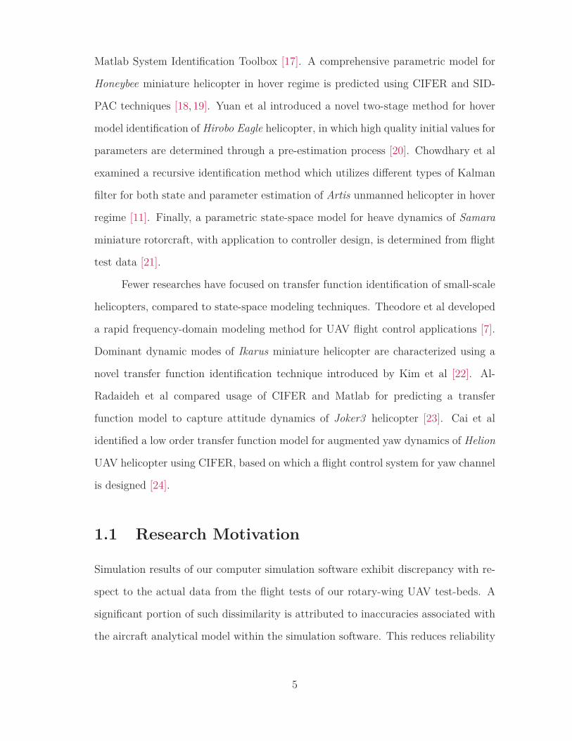
Fewer researches have focused on transfer function identification of small-scale
helicopters, compared to state-space modeling techniques. Theodore et al developed
a rapid frequency-domain modeling method for UAV flight control applications [7].
Dominant dynamic modes of Ikarus miniature helicopter are characterized using a
novel transfer function identification technique introduced by Kim et al [22]. Al-
Radaideh et al compared usage of CIFER and Matlab for predicting a transfer
function model to capture attitude dynamics of Joker3 helicopter [23]. Cai et al
identified a low order transfer function model for augmented yaw dynamics of Helion
UAV helicopter using CIFER, based on which a flight control system for yaw channel
is designed [24].
1.1 Research Motivation
Simulation results of our computer simulation software exhibit discrepancy with re-
spect to the actual data from the flight tests of our rotary-wing UAV test-beds. A
significant portion of such dissimilarity is attributed to inaccuracies associated with
the aircraft analytical model within the simulation software. This reduces reliability
5

level of any control design conducted based on the simulation software, and in turn
increases the need for further investigation, validation and tuning through the flight
tests which is expensive and time consuming. One solution to this problem is em-
ploying identification methods. Hence, the motivation of this work is to develop SID
tool for rotary-wing UAVs based on flight test measurements for the purpose of es-
tablishing more realistic and accurate simulation models, optimum system analysis,
and more efficient controller design.
The SID tool is designed to be embedded in the computer simulation software
available for the UAV platforms. This will help improving the reliability of simu-
lation by providing more accurate models for the aircraft, compared to analytical
models obtained from first principles. It is also considered as a preliminary stage in
developing a framework for online or in-flight system identification with applications
to fault-tolerant and adaptive control law design. Furthermore, the identified trans-
fer functions can be used in the control system design process to reduce number of
flight tests required for fine tuning the controllers on our UAV platforms.
The system identification tool, which is composed based on Matlab, gets the
input-output measurements, performs a data post-processing, and gives the best non-
parametric and parametric models of the system. This tool utilizes frequency-domain
Single Input/Single Output (SISO) identification techniques, namely frequency-response
and transfer function modeling, however with minimal modifications, it is extendable
for Multiple Input/Multiple Output (MIMO) state-space identification. In order to
verify its reliability, we tested the developed tool with real flight data, and compared
the results with CIFER, as a highly reliable tool in aircraft system identification.
The aircraft used for identification experiment is a Trex-700 commercially available
R/C helicopter designed by Align Corporation. The flight experiment is conducted
in hover regime for dominant dynamic modes, namely pitch and roll motions, by
MicroPilot Inc. The flowchart of Fig. 1.2 illustrates the logic behind our SID tool.
6
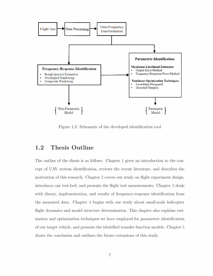
Figure 1.2: Schematic of the developed identification tool
1.2 Thesis Outline
The outline of the thesis is as follows. Chapter 1 gives an introduction to the con-
cept of UAV system identification, reviews the recent literature, and describes the
motivation of this research. Chapter 2 covers our study on flight experiment design,
introduces our test-bed, and presents the flight test measurements. Chapter 3 deals
with theory, implementation, and results of frequency-response identification from
the measured data. Chapter 4 begins with our study about small-scale helicopter
flight dynamics and model structure determination. This chapter also explains esti-
mation and optimization techniques we have employed for parametric identification
of our target vehicle, and presents the identified transfer function models. Chapter 5
draws the conclusion and outlines the future extensions of this study.
7

Chapter 2
Flight Experiment
From a technical point of view, this chapter summarizes flight experiment design for
model identification of a small-scale helicopter. Two types of excitation inputs are
designed, namely frequency sweep and doublet, in order to excite dominant attitude
dynamics of the flight vehicle. The frequency sweep excitation will be used for
model identification, and the doublet excitation will be employed in later flight tests
for model validation. Specifications of each input are summarized, and their minor
and major aspects are discussed. Moreover, our test-bed is introduced, and the key
practical considerations for conducting the identification flight test are elaborated.
Finally, the flight test results are presented, and the post-processing operations used
for conditioning the data is explained.
2.1 Introduction
Rotorcraft system identification is quite dependent upon acquired flight data as an
essential component of the identification. The richer the data, the more accurate and
reliable model can be identified. Hence, within all possible flight inputs which can
be used to excite the aircraft and collect the response data, those should be chosen
and designed that provide richer information about the system.
8

R/C helicopters, because of their high maneuverability, agility, and smaller
scale, have a quite different dynamic compared to large-scale or manned helicopters.
This certainly affects the way the system should be excited in a general flight ma-
neuver, or in an identification flight test. Different types of flight input have been
examined and proved to be reliable in the past for the purpose of system identifi-
cation of large-scale aircraft; however, for the case of unmanned aerial vehicle, and
more specifically model scale helicopters, the literature does not offer a single or an
optimum solution. Therefore, designing the flight input, in an optimum manner, is
desirable and is of very high importance.
In general, the experiment design is conducted in an iterative procedure, through
which an initial design is refined using the information obtained from non-parametric
identification and model analysis. In other words, within the input design procedure,
a non-parametric model will be identified, in order to check how good the aircraft
has been excited. Based on a simple model analysis, the input design parameters will
be refined and the values are updated. This procedure is repeated until the design
parameters converge to an optimum value in a practical sense [25]. A schematic of
the input design procedure is shown in Fig. 2.1. This work focuses on the initial
stage of input design. In this stage, firstly, different types of identification inputs
are reviewed. Then, based on our identification requirements, theoretical design
rules, practical constrains, and pilot opinion, a detailed design for excitation inputs
is accomplished. Furthermore, an operational plan is outlined for flight test imple-
mentation. The results of the initial input design will be used in order to conduct
flight experiment and collect measurement data.
9

Figure 2.1: Iterative procedure of input design
2.2 Scope of Input Design
For system identification of fixed-wing and rotary-wing flight vehicles, input exci-
tation can be categorized under two classes, heuristic and non-heuristic inputs [26].
Heuristic inputs are those applied mostly in frequency-domain identification meth-
ods, which have been widely used in rotorcraft model identification, and do not
require a priori knowledge of system dynamics. Piloted (or automated) frequency
sweep, impulse, and multi-sine (such as Shroeder-Phase, Mehra, and DUT) inputs
are classified as heuristic inputs. In contrary, designing non-heuristic inputs requires
some prior knowledge of dynamic behavior of the system. In addition to optimal
inputs, conventional multi-step inputs (such as doublet, 3211, 211, etc.) are cat-
egorized as non-heuristic inputs. These inputs are commonly used in time-domain
identification methods, as well as model verification [27]. Table 2.1 summarizes iden-
tification input types. A schematic of different identification inputs is illustrated in
Fig. 2.2.
In order to design a proper input signal, we have to recognize input parameters
10

first. Input shape or type is considered as the first variable in the design proce-
dure which is chosen in initial design step and is kept fixed during the design loop.
Frequency range, amplitude envelope, and maneuver time are the variables to be
adjusted during the iterative design procedure of the input after they have been
assigned a primary value in the initial design phase.
Table 2.1: Different types of excitation input used in aircraft system identification
Input Class Type Subcategory
Heuristic
Impulse One-sided Two-sided
Frequency Sweep Piloted Automated
Multi-Sine Shroeder-Phase Mehra DUT
Non-HeuristicMulti-Step Doublet 3211 211
Optimal Inputs Estimation Error Engineering Approach
Figure 2.2: Conventional input types used in aircraft system identification
In order to choose a proper input shape, two basic considerations have to be
taken into account: excitation capability of the desired dynamic mode and pilot
implementation constraints. Hence, for choosing an input type among all conven-
tional and optimal options, specification of the different inputs should be known first,
11
then a comparison has to be made, and finally the types that are in agreement with
identification requirements, which are capable of maximum excitation, and can be
practically applied by pilot, should be selected. By studying various identification
inputs, two types have been chosen. Piloted frequency sweep as well as doublet
multi-step input for model identification and verification, respectively. In the follow-
ing sections, specifications of these inputs are discussed. Also, the main reasons for
selecting these inputs are elaborated.
Frequency Sweep
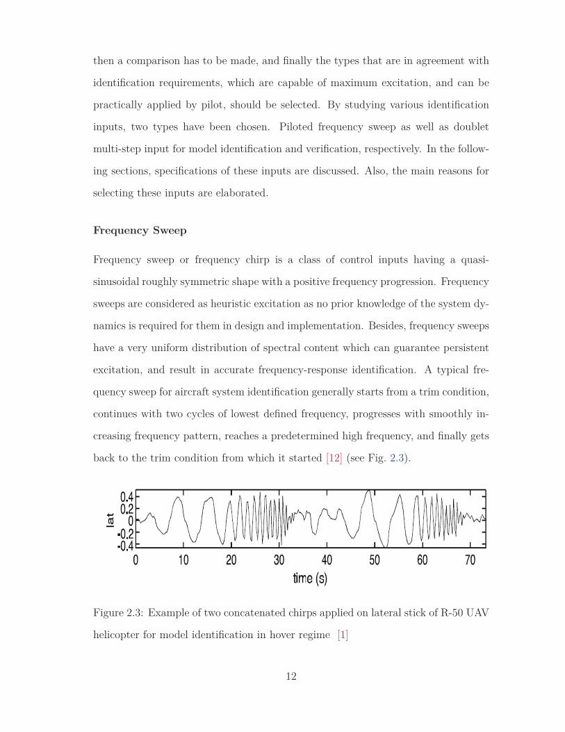
Frequency sweep or frequency chirp is a class of control inputs having a quasi-
sinusoidal roughly symmetric shape with a positive frequency progression. Frequency
sweeps are considered as heuristic excitation as no prior knowledge of the system dy-
namics is required for them in design and implementation. Besides, frequency sweeps
have a very uniform distribution of spectral content which can guarantee persistent
excitation, and result in accurate frequency-response identification. A typical fre-
quency sweep for aircraft system identification generally starts from a trim condition,
continues with two cycles of lowest defined frequency, progresses with smoothly in-
creasing frequency pattern, reaches a predetermined high frequency, and finally gets
back to the trim condition from which it started [12] (see Fig. 2.3).
Figure 2.3: Example of two concatenated chirps applied on lateral stick of R-50 UAV
helicopter for model identification in hover regime [1]
12

Having roughly symmetric time-history responses is a beneficial aspect of fre-
quency sweeps. It helps to maintain the aircraft centered around trim condition
and is important in determination of trim value in spectral analysis. In addition,
frequency sweep is a safe input from operational aspect as minimum and maximum
frequencies are predetermined which prevents overstressing aircraft modes such as
lightly damped structural modes. Key features for implementation of a piloted fre-
quency sweep are summarized in Table 2.2.
Table 2.2: Key specifications of piloted sweep for system identification
What is important What is NOT important
Start and end in trim Constant amplitude
Two complete long-period inputs Exact sinusoidal shape
Smooth increasing frequency progression Exact frequency progression
Rough symmetry about trim Exact repeatability
Non-swept inputs for off-axis channels Higher amplitude in high frequencies
However using frequency sweep can guarantee persistent and accurate identi-
fication results without having a priori knowledge of system, there are some minor
aspects regarding this class of input that should be considered. Having a wide band-
width can help enriching response information content; although, it can be critical
in minimum and maximum frequencies. In other words, it is hard to maintain flight
condition in low frequencies, and in higher frequencies, lightly damped structural
modes, or some aircraft system modes could be excited unintentionally. Besides,
for MIMO systems, using frequency sweep is not practical, so their usage is limited
to SISO systems. Moreover, frequency sweep requires considerably longer record
time compared to other identification inputs. Hence, using frequency chirp for cases
in which a short flight time is necessary (e.g. high-angle-of-attack aircraft) is not
feasible [12]. In Table 2.3, major and minor aspects for frequency sweeps are listed.
13

Table 2.3: Frequency sweep minor and major aspects
Major Aspects Minor Aspects
Easy pilot implementation Not suited for MIMO systems
Prior knowledge is not required Not optimum SID results
Persistent and reliable SID results Unintentional high frequencies excitation
Accurate SID results Hard to keep flight condition in low ω
Large bandwidth Long duration record time
Multi-Step input
Multi-step inputs are a combination of simple step pulses with different pulse width in
positive and reverse directions. In a pulse signal, which is the simplest way to excite
the oscillatory motion of aircraft, the control input is active for a certain amount
of time, then released for the aircraft to freely respond about its trim condition.
Doublets, 3211, 1123, 211 are different types of multi-step signals used in system
identification. Herein, the specification of doublet and 3211 multi-step inputs are
discussed as popular inputs in aircraft model identification and validation.
Figure 2.4: Examples of actual multi-step input: Excited lateral and longitudinal
sticks of BO-105 helicopter used for hover model validation [2]
Doublet input is a symmetrical two-sided pulse in which the control stick is
moved abruptly from trim position and held fixed for a predetermined time step Δt.
Then, in a symmetric fashion, the control is moved abruptly again in the reverse
14

direction and held fixed for the same amount of time, and finally, released quickly
to get back to its initial trim value. The 3211 multi-step input is similar to doublet
from two aspects: the sudden control reversal and the trim start and end points.
However, 3211 input composed of four linked pulses the width of which is varying
in a decreasing manner, i.e. 3Δt for the first pulse, 2Δt for the reversed pulse, and
two 1Δt for the doublet shape pulse at the end. Figure 2.4 depicts actual 3211 and
doublet inputs applied to helicopter system identification [25].
Doublet can be considered as square wave approximation of sine wave having
a broader bandwidth. However, its energy is more concentrated on the frequency
of the corresponding sine wave characterized by Δt. In designing doublet and 3211,
time step Δt is chosen based on the Eigen frequency of desired flight mode to be
excited which is known a priori. That is why these inputs are classified as non-
heuristic inputs. Time variations and multiple step reversals in 3211 input provide a
much broader bandwidth compared to the doublet input. Higher band width allows
for 3211 to adequately excite a band around natural frequency of the flight mode of
interest; however, doublet is more flight condition dependent. The 3211 input is also
called poor man’s frequency sweep for its similarity to frequency sweep in covering a
wide range of frequencies [28].
In helicopter system identification, doublet is generally used for model verifica-
tion, mainly because it is different enough from frequency sweep as a common input
for helicopter identification. This is good to assure that the identified model is not
dependent on a specific type of input. Doublets are also proved to be well suited as
directional input (rudder/pedal) in identification. Likewise, it has been proved that
3211 is more suitable as longitudinal input (elevator/cyclic pitch). Both doublet and
3211 are easier in execution than frequency sweep. Also, similar to frequency sweep,
in doublet and 3211, duration and exact shape is of second importance [12]. Com-
pared to doublet, 3211 is an asymmetrical input (4Δt positive pulse and 3Δt negative
15

pulse), which will affect the spectral analysis in finding the spectral estimate of trim
values. Similar to frequency sweep, larger duration of initial pulses in 3211 can cause
the aircraft to deviate a lot from trim condition which is not desirable. These minor
aspects of 3211 can be overcome using modified 3211, or using two linked 3211 with
the second one having reversed polarity [28]. Minor and major aspects of doublet
and 3211 are summarized in Table 2.4.
Table 2.4: Major and minor aspects of multi-step input design strategies
Doublet 3211
Major
Aspects
Easier pilot implementation than frequency sweep
Exact shape and pulse duration is of second importance
Suitable as directional input Suitable as longitudinal input
Suited for model verification Suited for model identification
Symmetric Wide band input
Minor
Aspects
A priori knowledge is required
Shorter band than 3211 Unstable response in low frequencies
Flight condition dependent Asymmetric
2.3 Input Detailed Design
The main input type chosen for the identification problem is frequency sweep for
couple of reasons. Firstly, frequency sweep is recognized as a very reliable input in
large-scale helicopter model identification. The use of frequency sweep in unmanned
helicopter identification has been also examined in some works in the past resulting in
persistent and reliable models [1]. Besides, as there is not enough information about
the target helicopter, Trex-700, frequency sweep as a broadband input covering a
wide frequency spectrum can be the optimum (not time-optimal) choice. Applying
16
frequency sweep requires a longer flight test, plus some consideration in execution
by pilot, which is not an issue in this work. Consulting with the pilot, some ideas for
implementation of the frequency sweep input are obtained, which are explained later
in this thesis (see section 2.5). Besides, optimal inputs are omitted from our choice as
they require an initial educated estimate of model parameters which is not available
in our case. Likewise, it is better to avoid using doublet inputs for identification
since doublets are more dependent on the flight mode being identified, and there is
not sufficient information about the system available. However, doublet can be used
for time-domain verification of the models identified using frequency sweep inputs,
because it is different enough from frequency sweep in shape and pattern, and it is
very simple and easy (easier than 3211 and frequency sweep) for pilot to apply.
2.3.1 Piloted Frequency Sweep
Design parameters of a piloted frequency sweep consist of frequency range of interest,
amplitude range, and record time. For determining frequency range, it is desired
to recognize minimum and maximum frequencies of interest to ensure acceptable
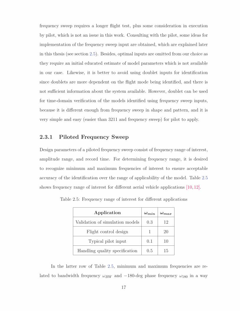
accuracy of the identification over the range of applicability of the model. Table 2.5
shows frequency range of interest for different aerial vehicle applications [10,12].
Table 2.5: Frequency range of interest for different applications
Application ωmin ωmax
Validation of simulation models 0.3 12
Flight control design 1 20
Typical pilot input 0.1 10
Handling quality specification 0.5 15
In the latter row of Table 2.5, minimum and maximum frequencies are re-
lated to bandwidth frequency ωBW and −180-deg phase frequency ω180 in a way
17

that ωmin = 0.5 ωBW and ωmax = 2.5 ω180, both of which can be determined from
frequency-response function of the system. As an example, ωBW and ω180 for bare
airframe of a helicopter have typical values of 1 and 6 rad/s respectively [12]. In
selection of frequency range for the input, the domain of application in addition to
feasibility of execution by pilot should be considered. For example, for validation
of simulation models, lower frequencies are of high importance; however, for flight
control design application high end frequency is more important. According to the
identification requirements, following the general guidelines stated in Table 2.5, and
having considered that the pilot is capable of applying inputs up to the frequency
of 2 Hz (≈ 12.5 rad/s), the frequency range is selected as follows. These values are
selected as an initial guess and will be fine-tuned in the iterative procedure for later
flight tests.
0.3 ≤ ω ≤ 12 rad/s (2.1)
According to a general guideline [12], frequency sweep record time has to be
equal or greater than a certain value proportional to maximum period of excitation
as Trec ≥ 4.5Tmax. Considering the initial value for minimum frequency (maximum
period), the record time is obtained as Trec = 90 s. As mentioned previously, a piloted
frequency sweep used for identification purpose requires to start in trim condition,
follows with two cycles of minimum frequency (0.3 rad/s in our case), covers the
frequencies between ωmin and ωmax smoothly, and finally, ends also in trim condition.
For both start and end of the input signal, 3 seconds of trim input is considered with
two initial low frequency cycles having the period of 20 seconds.
The amplitude of identification input should be strong enough at each time
step to be able to excite the dynamic mode of interest, i.e. it should be greater
than a minimum value. Besides, it cannot be greater than a certain value because
it might corrupt the linearity assumptions of the model. Following a general rule
of thumb [12], the control input has to be within the range of ± 10 - 20% of input
18

full range. From the aircraft response point of view, these lower and upper limits
for attitude angles should be ± 5 - 15 deg. In a same manner, angular rates should
lie within the range of ± 5 - 15 deg/s, and forward velocity should not exceed the
limits of ± 5 - 10 kn. The response of aircraft has to be kept within this predefined
envelope and inputs which might cause the response to exceed these ranges should
be avoided. This can be done with the help of data telemetry during flight test. It is
also recommended that signal amplitude starts and ends with a gradual phase-in and
phase-out respectively [12]. The results of the frequency sweep detailed design are
summarized in Table 2.6. Figure 2.5 illustrates a schematic of the designed frequency
sweep.
Table 2.6: Frequency sweep design specifications
Design Parameter Value Units
Frequency range 0.3 - 15 rad/s
Record time 90 s
Period of initial/final trim 3 s
Amplitude envelope ±10 - 20 %
Attitude response limitations ±10 - 15 deg
Angular rate limitations ±10 - 15 deg/s
Forward velocity limitations ±5 - 10 kn
2.3.2 Doublet Input
In designing the doublet input, the parameter to be selected is the time step of the
signal. Optimum range of frequencies of multi-steps is a range below and above the
natural frequency of the mode being excited. This frequency range is characterized
by the shape, duration, and time step of the multi-step. Based on a design rule of
19

0 10 20 30 40 50 60 70 80 90−30
−20
−10
0
10
20
30
Time, s
InputAmplitude,
%
Figure 2.5: Schematic of the designed frequency sweep
thumb [28], the time step for the doublet is given in terms of natural frequency of
the desired mode in equation (2.2).
Δtdblt = 0.5 Tosc = 3.142/ωn (2.2)
By knowing the period of oscillations of the flight mode a priori (Tosc), the time
step of the doublet input for exciting that mode can be determined. In our design,
we decided on an initial educated guess for the time step by studying multi-steps
used for identification of various rotary-wing and fixed-wing aircraft. In order to
find an initial guess for the time steps, multi-steps used for identification of Yamaha
R-50 are considered [9]. In that research, a combination of doublets and 3211 inputs
are used for identification of different modes of R-50 helicopter in hover and cruise
flight regimes. The time step of 3211 used for collective pitch stick is about 0.5 sec.
The time step of the doublets (Δtdblt) applied to cyclic inputs as well as directional
input varies between 1 to 2 seconds. Moreover, in LOES identification of Tu-144LL
fixed-wing aircraft [29], a 211 type of multi-step is used for longitudinal stick with
the time step of about 1.5 seconds. In another application for identification of the
DLR BO-105 helicopter [2], doublets applied as cyclic input have the time step of
20

about 1.5 seconds, and 3211 has the time step of approximately 1 second. Finally, a
series of linked doublets is used as the elevator input for identification of F-18 High
Alpha Research Vehicle [30] with the time step of roughly 0.75 s. A summary of
these information are collected in Table 2.7.
Table 2.7: Examples of multi-step inputs employed in aircraft system identification
Aircraft Input Type Δt sec
Yamaha R-50 UAV Helicopterdoublet 1-2
3211 0.5
DLR BO-105 Helicopterdoublet 1.5
3211 1
Tu-144LL Supersonic Aircraft 211 1.5
F-18 High Alpha Research Vehicle linked doublets 0.75
Finally, two linked doublets with reversed polarity are considered with a time
step adopted from similar aircraft data. Amplitude ranges will be the same as the
frequency sweep, i.e. ± 10 - 20% of the input full range. The results of the initial
design are summarized in Table 2.8. Figure 2.6 illustrates a schematic of the designed
doublet input.
0 2 4 6 8 10 12 14 16 18 20−25−20−15−10−50
5
10
15
20
25
Time, s
InputAmplitude,
%
Figure 2.6: Schematic of the designed doublet input
21

Table 2.8: Doublet design specifications
Design Parameter Value Units
Time step 2 s
Record time 20 s
Period of initial trim 3 s
Period of final trim 6 s
Amplitude envelope ±10 - 20 %
Attitude response limitations ±10 - 15 deg
Angular rate limitations ±10 - 15 deg/s
Forward velocity limitations ±5 - 10 kn
2.4 Introduction to the UAV Testbed
For flight test purpose of this research work, we have used a Trex-700 airframe
equipped with MP2128G2Heli MicroPilot autopilot. Trex-700 is a commercially
available unmanned helicopter designed by Align Corporation using a flybarless rotor
system, having approximate gross weight of 4200 g, main rotor diameter of 1602
mm, and tail rotor diameter of 281 mm, and utilizing a brushless electric motor,
and a collective-pitch rotor configuration [31]. Major dimensions of the vehicle are
illustrated in Fig. 2.7.
The autopilot is armed with 3 MEMS gyros to measure the angular rates of the
vehicle in the body-fixed frame. It is also equipped with 3 accelerometers to measure
translational accelerations, and a GPS and a Compass for navigation purpose. The
autopilot utilizes a Kalman filter to estimate the unknown and unmeasured states,
in order to compensate for the inaccuracies in the sensor measurements. Hence, the
angular rates as the output measurement extracted from the autopilot are not direct
sensor outputs, but corrected for bias error and sensor drift through an onboard
22

Figure 2.7: Trex-700 dimensions based on its operating manual
algorithm. The autopilot also utilizes a yaw-rate feedback system to augment the
stability of yaw dynamics. Except for the yaw mode, which requires a mandatory
control system, a Pilot-In-Control (PIC) flight test is performed for identification
experiment. The pilot cyclic and collective commands as input measurements are
measured through an onboard radio receiver system. The autopilot is located almost
at the center of gravity of the vehicle, and the data are logged at sampling frequency
of 30 Hz. Figure 2.8 depicts the flight-test vehicle equipped with MP2128G2Heli
autopilot.
2.5 Flight Test Implementation
The flight test for the purpose of system identification are fundamentally different
from general flight maneuvers for which pilots are trained. Pilots tend to control
23
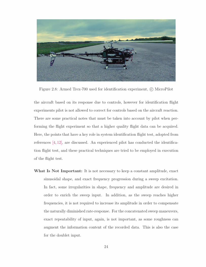
Figure 2.8: Armed Trex-700 used for identification experiment, c© MicroPilot
the aircraft based on its response due to controls, however for identification flight
experiments pilot is not allowed to correct for controls based on the aircraft reaction.
There are some practical notes that must be taken into account by pilot when per-
forming the flight experiment so that a higher quality flight data can be acquired.
Here, the points that have a key role in system identification flight test, adopted from
references [4, 12], are discussed. An experienced pilot has conducted the identifica-
tion flight test, and these practical techniques are tried to be employed in execution
of the flight test.
What Is Not Important: It is not necessary to keep a constant amplitude, exact
sinusoidal shape, and exact frequency progression during a sweep excitation.
In fact, some irregularities in shape, frequency and amplitude are desired in
order to enrich the sweep input. In addition, as the sweep reaches higher
frequencies, it is not required to increase its amplitude in order to compensate
the naturally diminished rate-response. For the concatenated sweep maneuvers,
exact repeatability of input, again, is not important, as some roughness can
augment the information content of the recorded data. This is also the case
for the doublet input.
24

What Is Important: Some irregularity in the piloted inputs are appreciated, how-
ever, there are some factors that are important and must be noted. Starting
from and finishing in the trim condition, emphasizing the higher periods (lower
frequencies) in first half of the record time, having a smooth frequency pro-
gression without rushing to higher frequencies, and not exceeding the high end
frequency are highly important in sweep excitation. The same rules apply for
doublet excitation.
Off-Axis Excitation: While the pilot is applying a sweep/doublet to one control
and monitoring the corresponding on-axis response, all other controls should be
kept roughly symmetrical to the reference flight condition in order to bound the
off-axis responses. For example, if the mode being excited is the short-period
pitch mode by applying a sweep to longitudinal cyclic control, it is desired to
keep lateral cyclic, collective and pedal controls symmetric with lowest possible
amplitude to maintain the off-axis responses within a reasonable range. In
other words, pilot should be advised to concentrate on the primary input, not
to correlate the on-axis responses with the secondary controls.
Task of the Copilot: Pilot-applied sweeps and doublets are best done when two
crews are involved, one in charge of the input and the other calling the tune.
The copilot should provide the timing indicators to assist the pilot in con-
ducting the flight test. The copilot can call out the time at certain times to
signal the pilot when the control stick should be at a certain position. For
the frequency sweep input, the pilot has to be signaled when the maximum
frequency is approached and when it is reached. Telemetry data are also useful
for monitoring the frequency progression in frequency sweep input.
Training, Practice, Safety: Experience has shown that pilots tend to increase the
amplitude while the frequency increases. It is also difficult for a pilot to judge
25

about frequencies beyond 2Hz. It is recommended that the pilot practices while
the vehicle is on the ground in order to realize the feel about the hand and feet
motion required. Applying the inputs in a simulation environment is helpful
as well. During the flight test, it is suggested that the pilot starts with simple
sine waves with constant low amplitude, and then try to increase the frequency
incrementally. It is necessary for the pilot to start the implementation of the
designed inputs only when enough confidence has been gained to enhance the
safety of flight test execution.
2.6 Flight Test Results
The flight test results used in this study belong to the excitation of pitch and roll
on-axis responses only. Two frequency sweeps are applied to longitudinal and lateral
cyclic inputs, denoted as δlon and δlat, respectively. The vehicle direct responses to
these controls, namely pitch-rate q and roll-rate p, are measured accordingly. The
measured data are passed through an anti-aliasing filter, and also corrected for effect
of sensor drift. The post-processing procedure involves conditioning the data using
a second-order low-pass filter with cut-off frequency of 25 rad/s, and removing the
average value from all signals. Mean-removal operation will significantly increase the
accuracy of identification in lower frequencies. Input-output data for longitudinal
and lateral modes are illustrated in figures 2.9 and 2.10, respectively.
26

0 5 10 15 20 25 30 35 40−100
−50
0
50
100
t, sec
δ lon,%
0 5 10 15 20 25 30 35 40−200
−100
0
100
200
t, s
q,deg/s
Figure 2.9: Flight test results: measured input-output for longitudinal mode
0 5 10 15 20 25 30−100
−50
0
50
100
t, sec
δ lat,%
0 5 10 15 20 25 30−200
−100
0
100
200
t, s
p,deg/s
Figure 2.10: Flight test results: measured input-output for lateral mode
27

Chapter 3
Frequency-Response Identification
In the previous chapter, the flight-test vehicle was introduced, and the procedure
for flight test execution and data collection is discussed. In this chapter, it is
aimed to estimate an accurate and reliable non-parametric model for longitudinal
and lateral dynamic modes of Trex-700 from the acquired flight data. This chapter
begins with an introduction on frequency-response system identification issue. Sec-
tions 3.2 and 3.3 shed light on the theoretical aspects of the techniques used in the
frequency-response identification. In Section 3.4, the identification results for Trex-
700 helicopter obtained using a developed Matlab code are acquired. The results
of the non-parametric models identified using CIFER toolbox are also given in this
section. Finally, Section 3.5 concludes this chapter by providing an analysis for the
identified models.
3.1 Introduction
Frequency-response system identification, also referred to as non-parametric model
identification, is a modeling approach which attempts to estimate frequency-response
function of a system from sampled input-output data. The frequency-response func-
tion is defined for any time-invariant system as the ratio of system output (response)
28

to system input (excitation) in frequency-domain. The term "frequency response"
is essentially referred to the steady-state response of a linear time-invariant system
when excited using a constant sine-wave input, which always results in a harmonic
response with the same frequency of the excitation, a certain phase shift, and a mag-
nified amplitude. This concept can be extended to a nonlinear time-invariant system
if the fact that any arbitrary input signal can be expressed in terms of its periodic
functions using Fourier series/transform is taken into account [32]. For a nonlin-
ear system, the frequency-response function is the best linear model of input-output
behavior which provides key information about the dynamic system characteristics.
The advantage of this representation of system dynamics is that no prior knowledge
and assumption for system structure or properties is required, except that the system
is time-invariant [12].
The frequency-response system identification is widely used for dynamic system
analysis, model validation for simulation, control system design, and more impor-
tantly, as a basis for parametric model identification [16] which is the main subject of
Chapter 4. In following sections, we will introduce the methods that are used for find-
ing an accurate estimate for the frequency-response function of a typical rotorcraft,
as a nonlinear system, from measured input-output data.
3.2 Time-Frequency Transformation
Finding frequency-response function from a time-history dataset, firstly requires for
the time-domain data to be transformed into the frequency-domain. The transfor-
mation methods commonly used in aircraft system identification are Discrete Fourier
Transform (DFT), Fast Fourier Transform (FFT), and Chirp Z-Transform (CZT).
The FFT is a quite faster method compared to the DFT, as it requires less data
29
points in calculations. However, the CZT is proved to be the most reliable and accu-
rate method for frequency-response estimation which provides high flexibility in the
selection of sample rates and frequency resolution [12].
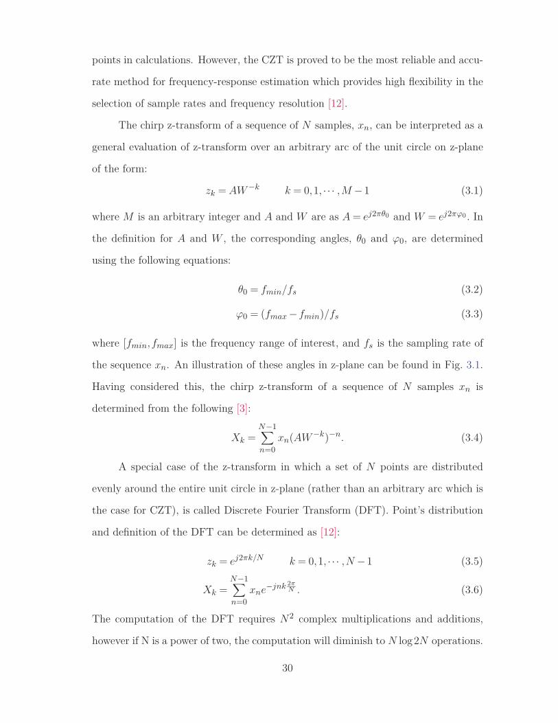
The chirp z-transform of a sequence of N samples, xn, can be interpreted as a
general evaluation of z-transform over an arbitrary arc of the unit circle on z-plane
of the form:
zk = AW −k k = 0,1, · · · ,M −1 (3.1)
where M is an arbitrary integer and A and W are as A = ej2πθ0 and W = ej2πϕ0 . In
the definition for A and W , the corresponding angles, θ0 and ϕ0, are determined
using the following equations:
θ0 = fmin/fs (3.2)
ϕ0 = (fmax −fmin)/fs (3.3)
where [fmin,fmax] is the frequency range of interest, and fs is the sampling rate of
the sequence xn. An illustration of these angles in z-plane can be found in Fig. 3.1.
Having considered this, the chirp z-transform of a sequence of N samples xn is
determined from the following [3]:
Xk =N−1∑n=0
xn(AW −k)−n. (3.4)
A special case of the z-transform in which a set of N points are distributed
evenly around the entire unit circle in z-plane (rather than an arbitrary arc which is
the case for CZT), is called Discrete Fourier Transform (DFT). Point’s distribution
and definition of the DFT can be determined as [12]:
zk = ej2πk/N k = 0,1, · · · ,N −1 (3.5)
Xk =N−1∑n=0
xne−jnk 2πN . (3.6)
The computation of the DFT requires N2 complex multiplications and additions,
however if N is a power of two, the computation will diminish to N log2N operations.
30

This evaluation of the DFT, which is much more efficient in calculations, is called Fast
Fourier Transform (FFT) [3]. A high accuracy evaluation of finite Fourier transform
is used in SIDPAC for the time-frequency transformation [33]. Similar to CIFER,
the chirp z-transform is employed as the transformation method in this study.
Figure 3.1: Illustration of CZT in z-plane [3]
3.3 Frequency-Response Function
In order to find the frequency-response function from the time-frequency transforma-
tion results, three methods are examined. Firstly, rough estimate of the frequency-
response function H(f) is obtained from rough spectral estimates. Secondly, smooth
frequency-response estimate H(f) is determined from smooth spectral quantities us-
ing so-called overlapped windowing method. An improved estimation of the frequency-
response function Hc(f) is obtained from taking a weighted average from several
individual frequency-response functions each of which acquired from evaluating win-
dowing method with a distinctive window length. The later method is called compos-
ite windowing which mixes the averaging benefits of smaller windows with dynamic
range advantages of larger windows.
31

3.3.1 Rough Estimation of Spectral Quantities
The outcomes of time-frequency transformation of a typical input signal u(t) and
output signal z(t), i.e. Fourier coefficients, U(f) and Z(f), introduce three important
spectral functions. These spectral functions, which are rough estimates of input
Power Spectral Density (PSD), output PSD, and input-output cross-spectrum (or
cross-PSD), are determined from the following equations, respectively.
Guu(f) = 2Trec
|U(f)| (3.7)
Gzz(f) = 2Trec
|Z(f)| (3.8)
Guz(f) = 2Trec
[U †(f)Z(f)
](3.9)
where U(f)† denotes the complex conjugate of the input Fourier Coefficient U(f) [34].
The PSD magnitude can also be displayed in power decibels as follows:
GuudB(f) = 10 log10(Guu(f)) (3.10)
After the rough estimates of spectral densities are found, the frequency-response
function H(f) can be estimated from either one of the following expressions:
H1(f) = Guz(f)Guu(f)
(3.11)
H2(f) = Gzz(f)Gzu(f)
(3.12)
These expressions are considered as unbiased estimations of the frequency-response
function provided that some assumptions about the measurement and process in-
put/output noise are taken into account. They require some assumptions about the
noises that might corrupted the time-domain signals. A general good assumption
for H1(f) expression in aerial vehicle applications accounts for the output noise i.e.
ν(t) �= 0, and neglects input measurement noise i.e. u(t) �= 0. The input noise asso-
ciated with unknown disturbances or unmeasured inputs, namely p(t), are indirectly
considered in the output noise ν(t) [12].
32

Figure 3.2: Measurement noise in input and output signals
3.3.2 Overlapped Windowing
In frequency-response estimation, one practical method which highly reduces the
effects of random error in spectral estimates is called overlapped windowing or Peri-
odogram. In this method, time-domain data is divided into shorter overlapping time
segments or windows of length Twin. Each segment is then multiplied by a window
tapering function w(t) in order to reduce the error associated with side-lob leakage
in spectral estimates. Then, Fourier coefficients for each weighted time segment are
determined separately. Finally, smooth estimate for the input signal, also referred to
as input autospectrum denoted by Guu(f), is obtained by averaging rough spectral
estimate of each individual window as expressed in the following:
Guu(f) = (1/clnr)nr∑
n=1Guu,k(f) (3.13)
where nr is the number of windows and cl is the correction factor for the energy
loss due to window tapering which depends upon the type of the window tapering
function w(t). The output autospectrum and cross-spectrum Gzz(f) and Guz(f) are
calculated similarly [12]. One tapering function that is commonly used in windowing
techniques is Hanning function, which is also the tapering function employed in
CIFER. A new research [35] shows that significant improvements in the results can
33

be achieved when a tapering function of the following form is used:
w(t) = sin(πt/Twin) (3.14)
which is referred to as half-sine function. Considering the aforementioned noise as-
sumption, in addition to considering that the existing output noise is uncorrelated to
input signal, one can determine the smooth frequency-response function from equa-
tion (3.5) by replacing rough spectral estimates with the smooth spectral estimates.
The challenge in the windowing technique is coming up with an optimum value
for the window length Twin. Because, larger windows provide good frequency res-
olution in expense of reducing the number of averages which causes an increase in
random error. While, shorter windows benefit from a lower random error in expense
of limiting the dynamic range. As per guideline [12], a window length selected for
time-domain data segmentation should be bounded in a range in which its lower and
upper limits are given as:
Trec
2 ≤ Twin ≤ 20 2π
ωmax(3.15)
where ωmax is the maximum frequency of the excitation. In this study, an average
value is chosen for window length, that is Twin = (Trec/2+40π/ωmax)/2.
3.3.3 Composite Windowing
There is not an optimal single window length for estimating spectral quantities. The
larger window provides higher frequency resolution with a more accurate identifica-
tion in lower frequencies, while the smaller window increases the number of averages
and reduces the random error accordingly in higher frequencies. Composite window-
ing technique is a solution to the challenge of window size selection.
In this method, the estimation for spectral quantities are improved by taking
a weighted average of multiple spectral estimates each of which acquired from eval-
uating Periodogram method with a different value for the window length. In this
34

study, 5 window sizes are chosen with equal spacing from one another in order to
cover the allowable range for Twin represented in equation (3.15).
In this approach, the smooth spectral quantities for each window size is cal-
culated separately, e.g. Guu,i for input autospecterum, and ith window size. Then,
they are combined in a weighted averaging manner in order to form a single accurate
and reliable composite response. The weighting function for each window i and each
frequency f is defined based on random error εr metric as follows (see section 3.3.4
for random error definition):
Wi =[
(εr)i
(εr)min
]−4(3.16)
where (εr)min is the minimum value for the random error of different windows length
at a certain frequency point.
As an example, the input composite autospectrum at each discrete frequency
is determined from:
Guuc =
nw∑i=1
W 2i Guu,i
nw∑i=1
W 2i
(3.17)
Having considered the aforementioned assumptions for input and output noise, the
composite frequency-response function can be calculated from the composite spectral
estimates as follows [12]:
Hc(f) = Guzc(f)Guuc(f)
. (3.18)
3.3.4 Accuracy Metrics
Two important products of the smooth frequency-response function are Coherence
function and normalized random error. coherence function γ2, which gets a value
between 0 and 1, is defined at each frequency point and determines how much the
output spectrum is linearly attributable to the input spectrum. A mathematical
35

expression for coherence function is given in equation (3.19). The expected normal-
ized random error in frequency-response magnitude and phase can be represented in
terms of the estimated coherence function as shown in equation (3.20).
γ2(f) = |Guz(f)|2|Guu(f)||Gzz(f)| (3.19)
εr(f) = Cε
√√√√(1−γ2)2ndγ2 (3.20)
The parameter Cε in equation (3.20) accounts for the window overlap, and nd shows
the number of independent time averages which is defined as nd = Trec/Twin [34].
Similarly, for composite windowing method, coherence function and random
error are determined from equations (3.19) and (3.20) by replacing the smooth esti-
mates with the composite estimates. However, in random error equation, the window
selection parameter nd is calculated at each frequency based on the weighted-average
window length at that frequency [12]:
Twin(f) =
nw∑i=1
W 2i Twini
nw∑i=1
W 2i
. (3.21)
In order to facilitate the comparison of two different identification methods
or tools using the accuracy metrics such as coherence function and random error,
relative difference of these metrics is computed. Equations (3.22) and (3.23) show
the formulation of the relative difference between accuracy metrics calculated for two
different identifications, the later for random errors, and the former for coherence
functions.
Δγ2 = γ21 −γ2
2max{γ2
1 ,γ22} (3.22)
Δεr = εr1 − εr2
min{εr1 , εr2} (3.23)
The denominator of the relative difference formulation is supposed to get the better
value (reference value), which corresponds to the higher accuracy in our case. Hence,
36

in equation (3.22), the difference between coherence functions is divided by the maxi-
mum coherence value. Also, in equation (3.23), the difference between random errors
is divided by the minimum random error value. This is due to direct and inverse
relations that coherence function and random error have with accuracy, respectively.
3.4 Identification of the Model
In order to find a nonparametric model for the flight vehicle, Trex-700, from flight
test data, a Matlab code is developed. The processed input-output time-domain
data for longitudinal and lateral modes are fed to the code. The program estimates
the frequency-response function by employing three different methods presented in
the previous section, i.e. rough estimation, overlapped windowing, and composite
windowing. The program is quite capable of estimating a SISO non-parametric model
for any set of input-output data, and it can be extended for MIMO identification. A
schematic of the non-parametric SID tool is illustrated in Fig. 3.3.
Figure 3.3: Schematic of non-parametric SID tool
The same set of data are fed to CIFER non-parametric identification packages
(namely FRESPID and COMPOSIT) to estimate a separate model for comparison.
The results from CIFER and the developed Matlab code are presented in this section
in the form of spectral functions, frequency-response function, and accuracy metrics.
In order to assist the results comparison, relative difference between the accuracy
37

metrics obtained from CIFER and the developed SID tool are given in this section.
3.4.1 Longitudinal Dynamics
The dataset used for the identification of longitudinal mode consists of longitudinal
cyclic δlon as the input, and pitch-rate q as the output. The spectral functions, i.e.
input, output, and cross-PSDs for longitudinal short-period mode are illustrated in
Fig. 3.4. The results for frequency-response estimates from three aforementioned
methods in form of Bode plot are depicted in Fig. 3.5, along with the corresponding
accuracy metrics. Figure 3.6 shows the identification results obtained from the de-
veloped code and CIFER. Figure 3.7 provides the accuracy measures to be used for
validating each identified model, and comparing the results with one another.
100 101−20−10
0
10
20
30
40
ω, rad/s
Guu,dB
roughsmoothcomposite
100 101−20−10
0
10
20
30
40
50
ω, rad/s
Gzz,dB
100 101−10
0
10
20
30
40
ω, rad/s
|Guz|,dB
Figure 3.4: Estimated spectral functions for pitch motion
38

100 101−25−20−15−10−505
101520
ω, rad/s
|H|,dB
roughsmoothcomposite
100 101−1400−1200−1000−800−600−400−200
0
ω, rad/s
�H,deg
100 1010
0.10.20.30.40.50.60.70.80.91
ω, rad/s
γ2
100 1010
0.2
0.4
0.6
0.8
1
1.2
1.4
ω, rad/s
ε r
Figure 3.5: Estimated frequency-response function for pitch motion
39

100 10110
15
20
25
30
35
40
ω, rad/s
Guu,dB
CODECIFER
100 10110
15
20
25
30
35
40
ω, rad/s
Gzz,dB
100 1015
10
15
20
25
30
35
40
ω, rad/s
|Guz|,dB
100 101−14−12−10−8−6−4−20246
ω, rad/s
|H|,dB
100 101−260−240−220−200−180−160−140
ω, rad/s
�H,deg
Figure 3.6: Identification results for longitudinal mode
40

100 1010
0.2
0.4
0.6
0.8
1
ω, rad/s
γ2
CODECIFER
100 101−0.4−0.2
0
0.2
0.4
0.6
0.8
1
ω, rad/s
Δγ2
100 1010
0.2
0.4
0.6
0.8
1
1.2
1.4
ω, rad/s
ε r
100 101−2.5−2
−1.5−1
−0.50
0.5
ω, rad/s
Δε r
Figure 3.7: Accuracy metrics for longitudinal mode identification
41

3.4.2 Lateral Dynamics
The dataset used for the identification of lateral mode consists of lateral cyclic δlat as
the input, and roll-rate p as the output. The spectral functions, i.e. input, output,
and cross-PSDs for lateral roll mode are illustrated in Fig. 3.8. The results for
frequency-response estimation in form of a Bode plot are depicted in Fig. 3.9, along
with the corresponding accuracy metrics. Figure 3.10 shows the identification results
obtained from the developed code and CIFER. Figure 3.11 provides the accuracy
measures to be used for validating each identified model, and comparing the results
with one another.
100 101−30−20−10
0
10
20
30
ω, rad/s
Guu,dB
roughsmoothcomposite
100 101−10
0
10
20
30
40
ω, rad/s
Gzz,dB
100 101−20−10
0
10
20
30
ω, rad/s
|Guz|,dB
Figure 3.8: Estimated spectral functions for roll motion
42

100 101−20−10
0
10
20
30
40
50
ω, rad/s
|H|,dB
roughsmoothcomposite
100 101−1000
−500
0
500
ω, rad/s
�H,deg
100 1010
0.10.20.30.40.50.60.70.80.91
ω, rad/s
γ2
100 1010
0.20.40.60.81
1.21.41.61.82
ω, rad/s
ε r
Figure 3.9: Estimated frequency-response function for roll motion
43

100 1010
5
10
15
20
25
ω, rad/s
Guu,dB
CODECIFER
100 10110
15
20
25
30
ω, rad/s
Gzz,dB
100 1010
5
10
15
20
25
30
ω, rad/s
|Guz|,dB
100 101−10−50
5
10
15
ω, rad/s
|H|,dB
100 101−100−80−60−40−20
0
20
ω, rad/s
�H,deg
Figure 3.10: Identification results for lateral mode
44

100 1010.2
0.4
0.6
0.8
1
ω, rad/s
γ2
CODECIFER
100 101−0.1
0
0.1
0.2
0.3
0.4
0.5
0.6
ω, rad/s
Δγ2
100 1010
0.1
0.2
0.3
0.4
0.5
0.6
0.7
ω, rad/s
ε r
100 101−2
−1.5−1
−0.50
0.5
ω, rad/s
Δε r
Figure 3.11: Accuracy metrics for lateral mode identification
45

3.5 Analysis and Discussion
As a general rule of thumb, γ2 ≥ 0.6 and εr ≤ 0.2 demonstrate acceptable accuracy
in frequency-response estimation [12]. It is worth mentioning that in the method
used for rough estimation of the frequency-response function, which can be also
interpreted as a windowing technique with one rectangular window (Twin = Trec),
coherence function gives a meaningless value of 1 for all frequency points. So, the
coherence function and random error estimation are only considered as accuracy
measures when a non-rectangular windowing technique is utilized.
Firstly, we consider the comparison between the results of three different tech-
niques exploited for frequency-response identification. For both longitudinal and lat-
eral dynamics, the PSD plots of Figs. 3.4 and 3.8 show the superiority of the smooth
and the composite spectral estimates over the rough estimation of spectral functions.
It can be translated into the ability of the windowing techniques in eliminating the
effects of random noise in spectral estimates. In magnitude plots of Figs. 3.5 and 3.9,
the rough estimation results follow the trend of two other techniques with some fluc-
tuations. However, for the phase plots of the same figures, the rough estimation is
unable to provide an acceptable estimate.
In order to compare the smooth and composite estimations of the frequency-
response function, we can refer to the accuracy metric plots of Figs. 3.5 and 3.9, for
longitudinal and lateral dynamics, respectively. For the pitch motion, in frequency
range of 1 − 2 rad/s, the overlapped windowing gives a slightly better result. For
everywhere else in the spectrum, composite windowing provides more accuracy, i.e.
more coherence and less random error. For the roll motion, composite windowing
is superior throughout the whole spectrum, and is significantly better in frequency
ranges of 0.3−2 and 7−9 rad/s. Hence, for both dynamic modes, identified models
obtained from the composite windowing technique are more reliable, hence chosen
for comparison with CIFER identified models.
46

Next, we compare the non-parametric models acquired from the developed
SID tool and CIFER. The PSD plots for both dynamic modes depict a systematic
error between our results and CIFER’s, as can be seen in Figs. 3.6 and 3.10. In
the magnitude and phase plots of the same figures, the results of both tools closely
follow one another in mid and high frequencies (frequency range of 1 − 12 rad/s);
however, there is a considerable offset between low frequency results (frequency range
of 0.3−1 rad/s).
In order to verify the fidelity of the identified models, we refer to the accuracy
metrics of Figs. 3.7 and 3.11, for longitudinal and lateral modes, respectively. For
longitudinal dynamics, our results are more accurate in 0.3−0.5 rad/s, and CIFER
gives better results in 0.5 − 2 rad/s. For the mid and high frequencies (frequency
range of 2 − 12 rad/s) the results are only slightly different as can be seen in near-
zero values for Δγ2 and Δεr in that spectrum. For lateral dynamics, however, the
code provides higher coherence and lower random error in low and high frequencies
(0.3 − 1 and 2 − 12 rad/s), and CIFER results are inferior except for the range of
1−2 rad/s.
Overall, the acceptable accuracy is achieved in the frequencies beyond 0.7 rad/s
for the longitudinal mode, and 0.4 rad/s for the lateral mode. The coherence func-
tion and random error estimations for lateral dynamics in the range of 7 − 9 rad/s
are way beyond the acceptable range, which can be seen essentially in the poor ex-
citation of lateral cyclic input. According to the accuracy measures, and based on
the comparison with CIFER, it can be concluded that the developed Matlab code
can successfully estimate accurate non-parametric models for longitudinal and lateral
dynamics of Trex-700 in almost entire frequency range of interest.
47

Chapter 4
Parametric Model Identification
This chapter addresses the techniques required for acquiring a minimal adequate
parametric model for dominant dynamics of the UAV helicopter testbed, Align Trex-
700, from flight test data. Previously, in Chapter 3, a non-parametric model identifi-
cation method was examined to find an unbiased estimate of the frequency-response
function for longitudinal and lateral dynamics. Similar to Chapter 3, the parametric
modeling techniques of this chapter are implemented in a SISO frequency-domain
identification for on-axis longitudinal and lateral responses.
This chapter is organized as follows. The opening Section 4.1 gives a brief
explanation for parametric model identification. Section 4.2 introduces Low Order
Equivalent System (LOES) model identification as a type of parametric identification
approach. Section 4.3 reviews first-principle modeling techniques used for developing
a proper model structure to capture the flight dynamics of small-scale helicopters.
In Sections 4.4 and 4.5, two parameter estimation techniques, plus two proposed
solution routines will be described from a theoretical point of view. Section 4.6
contains parametric model identification results for Trex-700. The last Section 4.7
concludes this chapter.
48
4.1 Introduction
Parametric model identification of an aircraft aims to find an accurate and reliable
estimate of the unknown parameters, i.e. aerodynamic derivatives, based on which
the linear aircraft equations of motion are formulated. This can be implemented in
frequency-domain by fitting a known model structure with unknown parameters to
the frequency-domain transformation of the measured input-output data. The iden-
tification problem can be degraded to a parameter estimation problem if the model
structure, whether a state-space formulation or a transfer function representation, is
known a priori. The state-space formulation is dominantly used for finding a com-
plete model, including most of the aerodynamic derivatives, typically in a MIMO
identification procedure. A transfer function formulation, however, attempts to esti-
mate the key parameters of major dynamic modes, and mostly used in a SISO model
identification [10,12].
4.2 LOES Modeling
LOES modeling is a type of transfer function modeling which attributes system input
and output with a linear relation, including an exponential delay term associated with
the input. The concept of LOES was introduced originally in the 1970s for aircraft
handling quality purposes, where a low order transfer function was fitted to a high-
order frequency-response obtained from a high-order system [29]. An extension of
LOES models was later implemented in parametric system identification of flight
vehicles with a similar approach, in addition to including nonlinearities as well as
high-order effects in the delay term. A typical third-order LOES model is shown in
equation (4.1):
T (s) = b0s2 + b1s+ b2a0s3 +a1s2 +a2s+a3
e−τs. (4.1)
49
LOES modeling is considered as an intermediate step in the model identification
of an aircraft, as it provides information about fundamental dynamic characteristics,
and estimates parameters associated with dominant dynamic modes. A comprehen-
sive dynamic model, as an ultimate goal in modeling, accounts for all dynamic modes,
and requires many measurements of the aircraft states. The significance of LOES
models, however, lies in the ability to approximate a high-order complex aircraft
response to pilot input with minimum adequate parameters in the form of a transfer
function, which can be interpreted and analyzed more readily. Hence, they are found
to be quite sufficient for a wide range of applications, such as aircraft development,
subsystem modeling, structural mode determination, control law design validation,
flight mechanics characterization, and simulation [10,12].
The central task in LOES parametric model identification is to find a proper
model structure for desired dynamic modes with physically meaningful parameters.
The rest requires a parameter estimation technique to approximate those unknown
parameters. However, the truncation of highly complex and coupled helicopter dy-
namics into a low order model requires a thorough knowledge about flight dynamics
of rotorcraft, and is not an easy task. Hence, we need to shed light on principles
of rotorcraft dynamics before we proceed. An overview of model development of
small-scale helicopters, plus the model forms chosen for this work, are discussed in
the next section.
4.3 Rotorcraft Dynamics
The dynamical behavior of a conventional helicopter is dominated by main and tail
rotor systems, where aerodynamic forces and moments are produced and controlled
through angular and aeroelastic movements of the rotating blades. The resulting
50

forces and moments will then act on the helicopter body, and cause the vehicle to
translate and rotate simultaneously in six degrees of freedom. The main rotor blades
are controlled through a swashplate mechanism which transmits the actuator move-
ments, fixed to the body, to the blades revolving at a very high speed. The actuators
are commanded by helicopter major controls, which consist of collective, longitudinal
and lateral cyclic, and tail rotor inputs. Fig. 4.1 illustrates the swash plate mecha-
nism of Align Trex-700 used as the testbed for this research work.
Figure 4.1: Swashplate mechanism of Align Trex-700, c© MicroPilot
The rotor system actuators aim to adjust pitch angle of the blades. The pitch
angle, also referred to as feathering angle, is the rotation of the blade around its span.
An increase in the pitch angle causes the rotating blades to face the air at a relatively
higher angle of attack and increases the lift accordingly. The collective control apply
the same pitch angle to all the blades simultaneously, and is the primary source of lift
and thrust forces. The cyclic controls adjust the pitch angle of the main rotor blades
different from one another in order to produce longitudinal and lateral moments.
51

The tail rotor control regulates the pitch angle of the tail rotor blades similar to the
collective control in order to generate directional moment.
The helicopter responds to the controls in a multi-axis behavior, where a single-
axis control can change the position and attitude in multiple axes. Yet, a significant
weight of the controls is given to on-axis dynamics1. The rotor system also reacts to
the main rotor controls by adjusting coning and tilting angles of the rotor disk (also
referred to as tip-path plane) in multiple harmonics. Fig. 4.2 shows a schematic view
for the dominant harmonic of the rotor system response to the controls.
Figure 4.2: Rotor blades flapping motion [4]
4.3.1 Rigid-Body Model
A mathematical expression for helicopter flight dynamics can be developed from first
principles where the aircraft is modeled using fundamental laws of mechanics such
as Newton-Euler equations [4, 36, 37]. The nonlinear model obtained from generic
equations of motion is comprised of translational and rotational dynamics of the
rigid-body, which is exposed to external forces and moments due to aerodynamics,
propulsion, and gravity. The key task in identification of the model for flight vehi-
cles is finding an accurate expression for aerodynamic forces and moments in terms
of aircraft dynamic and control variables [38]. The collected equations of motion1On-axis responses for collective, longitudinal and lateral cyclic, and tail rotor inputs are con-
sidered as vertical velocity, longitudinal, lateral, and directional attitudes, respectively.
52
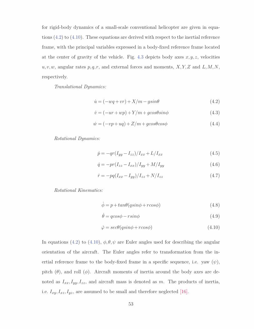
for rigid-body dynamics of a small-scale conventional helicopter are given in equa-
tions (4.2) to (4.10). These equations are derived with respect to the inertial reference
frame, with the principal variables expressed in a body-fixed reference frame located
at the center of gravity of the vehicle. Fig. 4.3 depicts body axes x,y,z, velocities
u,v,w, angular rates p,q,r, and external forces and moments, X,Y,Z and L,M,N ,
respectively.
Translational Dynamics:
u = (−wq +vr)+X/m−gsinθ (4.2)
v = (−ur +wp)+Y/m+gcosθsinφ (4.3)
w = (−vp+uq)+Z/m+gcosθcosφ (4.4)
Rotational Dynamics:
p = −qr(Iyy − Izz)/Ixx +L/Ixx (4.5)
q = −pr(Izz − Ixx)/Iyy +M/Iyy (4.6)
r = −pq(Ixx − Iyy)/Izz +N/Izz (4.7)
Rotational Kinematics:
φ = p+ tanθ(qsinφ+ rcosφ) (4.8)
θ = qcosφ− rsinφ (4.9)
ϕ = secθ(qsinφ+ rcosφ) (4.10)
In equations (4.2) to (4.10), φ,θ,ψ are Euler angles used for describing the angular
orientation of the aircraft. The Euler angles refer to transformation from the in-
ertial reference frame to the body-fixed frame in a specific sequence, i.e. yaw (ψ),
pitch (θ), and roll (φ). Aircraft moments of inertia around the body axes are de-
noted as Ixx, Iyy, Izz, and aircraft mass is denoted as m. The products of inertia,
i.e. Ixy, Ixz, Iyz, are assumed to be small and therefore neglected [16].
53

Figure 4.3: Helicopter body-fixed frame [4]
4.3.2 Extension of the Rigid-Body Model
The six Degree-Of-Freedom (6 DOF) rigid-body model does not suffice for capturing
the rotorcraft flight dynamics completely. Higher order effects, mostly due to rotor
blades aeroelasticity, must be considered in order to improve the model fidelity.
A well-known extension of the 6 DOF model, which accounts for simplified rotor
dynamics in addition to the rotor-body couplings, is called hybrid model [39]. The
hybrid model, which was originally developed for full-scale helicopters, was adopted
for model-scale rotorcrafts by Mettler [16]. This model aims to capture the dominant
dynamic modes of the rotor system by modeling the blades flapping motion through
the tilt angles of the tip-path-plane in the longitudinal and lateral directions, denoted
as a and b, respectively (see Fig. 4.2). This model is presented in following equations:
Simplified Rotor Dynamics:
a = −γΩ16 a+
kβ
2ΩIβb− q + γ
16p−Θa (4.11)
b = −γΩ16 b− kβ
2ΩIβa−p− γ
16p+Θb (4.12)
where Iβ is the moment of inertia of the blade about the flapping hinge, kβ is the
flapping hinge restraint spring constant, γ is the blade Lock number, Ω is the rotor
speed, and Θa and Θb are the blade pitch/feathering angles in longitudinal and
54

lateral directions, respectively.
Along with modeling the rigid-body and the rotor dynamics, a feedback system
which is commonly used to augment the stability of the yaw channel has to be
modeled. It is quite well known that the yaw dynamics of rotorcrafts with tail rotor
configuration is highly sensitive to controls (see equation (4.7)). This is mainly due
to the large size of the tail beam, where small changes in rotational speed of the main
rotor, or pitch angle of the tail-rotor blades can produce a huge yawing moment (N).
This sensitivity is even more extreme for unmanned helicopters with faster dynamics
and smaller size, which makes their manual control quite challenging. Hence, it is
essential for most of small-scale helicopters to be equipped with a yaw-rate gyro in
order to enhance their yaw stability and handling qualities [24]. A simple first-order
model is used to capture the effect of this feedback system:
Yaw Damping System:
rfb = −Krfbrfb +Krr (4.13)
where rfb is the yaw rate gyro feedback, and Krfband Kr are the feedback gains.
4.3.3 Model Linearization
The aforementioned set of nonlinear equations (4.2) to (4.10) can be linearized around
a reference/trim flight condition using small disturbance theory, where the states,
forces, and moments of the system are replaced by small perturbations around their
trim values [40]. For example, the vertical translational velocity w is replaced by
Δw according to w = w0 + Δw, in which w0 refers to the trim vertical velocity.
Hereafter, the Δ symbol is dropped from all variables for simplicity. Furthermore,
the aerodynamic forces and moments, denoted as X,Y,Z and L,M,N respectively,
can be expressed in terms of the aircraft states and control inputs by employing a
linear Taylor Series Expansion [41]. The basic helicopter control variables consist of
55

the main rotor collective pitch δcol, the tail rotor collective pitch δped, the longitudinal
cyclic input δlon, and the lateral cyclic input δlat. As an example, for the longitudinal
moment component M one can get
M = ∂M
∂uδu+ ∂M
∂wδw + ∂M
∂qδq + · · ·+ ∂M
∂δlonδlon + · · · (4.14)
where the partial derivatives of M with respect to the states and controls are called
stability and control derivatives, or aerodynamic derivatives, which are abbreviated
as follows:∂M
∂δlon= Mlon. (4.15)
It should be noted that not all of the states and controls contribute in each aerody-
namic force and moment. Associating forces and moments to the variables by which
they are altered is the principle of the parametric system identification, which is also
referred to as model structure determination.
The complete linearized equations of motion for a flybarless small-scale heli-
copter is collected in a state-space form in equation (4.16). In this differential equa-
tion, the system matrix A contains the stability derivatives, and the input matrix B
contains control derivatives. Also, x and u are state and input vectors, respectively.
x = Ax+Bu (4.16)
where the state vector is
x = [u,v,w,p,q,r,φ,θ,a,b,rfb]T (4.17)
and the input vector is
u = [δlat, δlon, δped, δcol]T (4.18)
56

A =
⎡⎢⎢⎢⎢⎢⎢⎢⎢⎢⎢⎢⎢⎢⎢⎢⎢⎢⎢⎢⎢⎢⎢⎢⎢⎢⎢⎢⎢⎢⎢⎢⎢⎢⎢⎢⎢⎢⎢⎢⎣
Xu 0 0 0 0 0 0 −g Xa 0 0
0 Yv 0 0 0 0 g 0 0 Yb 0
0 0 Zw 0 0 Zr 0 0 Za Zb 0
Lu Lv 0 0 0 0 0 0 0 Lb 0
Mu Mv 0 0 0 0 0 0 Ma 0 0
0 Nv Nw Np 0 Nr 0 0 0 0 Nrfb
0 0 0 1 0 0 0 0 0 0 0
0 0 0 0 1 0 0 0 0 0 0
0 0 0 0 −1 0 0 0 −1τf
Ab
τf0
0 0 0 −1 0 0 0 0 Ba
τf
−1τf
0
0 0 0 0 0 Kr 0 0 0 0 Krfb
⎤⎥⎥⎥⎥⎥⎥⎥⎥⎥⎥⎥⎥⎥⎥⎥⎥⎥⎥⎥⎥⎥⎥⎥⎥⎥⎥⎥⎥⎥⎥⎥⎥⎥⎥⎥⎥⎥⎥⎥⎦
(4.19)
B =
⎡⎢⎢⎢⎢⎢⎢⎢⎢⎢⎢⎢⎢⎢⎢⎢⎢⎢⎢⎢⎢⎢⎢⎢⎢⎢⎢⎢⎢⎢⎢⎢⎢⎢⎢⎢⎢⎢⎢⎢⎣
0 0 0 0
0 0 0 0
0 0 0 Zcol
0 0 0 0
0 0 0 0
0 0 Nped Ncol
0 0 0 0
0 0 0 0Alat
τf
Alon
τf0 0
Blat
τf
Blon
τf0 0
0 0 0 0
⎤⎥⎥⎥⎥⎥⎥⎥⎥⎥⎥⎥⎥⎥⎥⎥⎥⎥⎥⎥⎥⎥⎥⎥⎥⎥⎥⎥⎥⎥⎥⎥⎥⎥⎥⎥⎥⎥⎥⎥⎦
(4.20)
This formulation is originally developed by Mettler [15] for model identification
of Yamaha R-50 helicopter in hover flight regime. A similar model for cruise flight
57

regime is also addressed in reference [15]. This realization of rotorcraft dynamics
showed promise for modeling various model-scale helicopters as it is used extensively
in recent literature [1,7,14,18–20,42,43]. Other quantification of helicopter linearized
model accounting for higher order effects, such as rotor inflow dynamics, blade lead-
lagging motion, and stabilizer bar dynamics can be found in references [8,22,44,45].
The resulting simplified model is considered as local model, since it is only valid for
the specific flight condition about which the model is linearized. A general linear
model can be obtained by developing multiple set of local models in order to cover
the entire flight envelope [16].
4.3.4 LOES Model Structure
As mentioned earlier, the LOES identification of on-axis dynamics for our target
vehicle is desired in this chapter. With the insight gained from analytic modeling of
helicopter dynamics in Section 4.3, we are now able to determine physically meaning-
ful model structures for on-axis responses due to controls. Once the model structure
is established, in other words, once the decision about the inclusion of the effective
aerodynamic derivatives has been made, the model identification problem simply
becomes a parameter estimation problem. The on-axis dynamics for a conventional
helicopter composed of:
• Heave mode: Vertical velocity to main rotor collective, w/δcol
• Dutch-roll mode: Roll-rate response to lateral cyclic, p/δlat
• Short-period mode: Pitch-rate response to longitudinal cyclic, q/δlon
• Yaw mode: Yaw-rate response to tail rotor collective, r/δped
In order to obtain transfer function representation of these dynamic modes,
we require to further simplify the fully coupled hybrid model of equation (4.16),
which describes the fuselage, rotor, and feedback system dynamics. This can be
58

accomplished if two major assumptions are made. First, we assume that airflow
around the rotor blades is quasi-steady2. This will allow us to break down the rotor
dynamics into transient and steady-state responses. We will then include the rotor
transient dynamics in an equivalent time delay associated with inputs, denoted as τ .
Moreover, the rotor steady-state dynamics will be modeled as equivalent stability
and control derivatives of the rigid-body [15].
The other assumption for simplifying the model of equation (4.16) is neglecting
cross-axis coupling in the rigid-body equations, and splitting them into longitudinal
and lateral/directional dynamics [12]. The resulting decoupled models are a good
approximation for capturing the dominant dynamic modes of the helicopter. It is
worth recalling that, during the identification flight experiment, the pilot commands
one control input at a time. The secondary controls will be kept in the lowest
allowable amplitude not to correlate on-axis and off-axis responses with one another.
In other words, except for the primary control and response, the rest of aircraft
states and controls will have small variations. Therefore, the terms corresponding to
off-axis dynamics can be dropped and the equations can be decoupled.
The longitudinal dynamics are described with state vector xlon, and control
vector ulon in equation (4.21). Similarly, the lateral/directional dynamics are ex-
pressed with state vector xlat, and control vector ulat in equation (4.22). System
matrices F lon and F lat, and input matrices Glon and Glat, contain the equivalent
aerodynamics derivatives for longitudinal and lateral modes.
xlon = F lonxlon +Glonulon (4.21)
xlat = F latxlat +Glatulat (4.22)
2Quasi-steady flow assumes that the airflow around the aircraft, as a result the aerodynamicforces and moments, change instantaneously when the flight vehicle is disturbed from its trimcondition [46].
59

where the state and control vectors are given as:
xlon = [u,w,q]T (4.23)
xlat = [v,p,r,rfb]T (4.24)
ulon = [δlon(t− τp), δcol(t− τh)]T (4.25)
ulat = [δlat(t− τr), δped(t− τy)]T (4.26)
in which τp, τr, τy, and τh are equivalent time delay for pitch, roll, yaw, and heave
motions. The system and input matrices are given in the following:
Flon =
⎡⎢⎢⎢⎢⎢⎢⎣
Xu 0 Xq
0 Zw 0
Mu 0 Mq
⎤⎥⎥⎥⎥⎥⎥⎦
Glon =
⎡⎢⎢⎢⎢⎢⎢⎣
Xlon 0
0 Zcol
Mlon 0
⎤⎥⎥⎥⎥⎥⎥⎦
(4.27)
Flat =
⎡⎢⎢⎢⎢⎢⎢⎢⎢⎢⎢⎣
Yv Yp 0 0
Lv Lp 0 0
Nv Np Nr Nrfb
0 0 Kr Krfb
⎤⎥⎥⎥⎥⎥⎥⎥⎥⎥⎥⎦
Glat =
⎡⎢⎢⎢⎢⎢⎢⎢⎢⎢⎢⎣
Ylat 0
Llat 0
0 Nped
0 0
⎤⎥⎥⎥⎥⎥⎥⎥⎥⎥⎥⎦
(4.28)
The transfer function form of the dominant dynamic modes are obtained by
taking a Laplace Transform from equations (4.21) and (4.22).
Heave Mode:w
δcol= Zcol
s−Zwe−τ2s (4.29)
Short-Period Mode:
q
δlon= (Mlon)s+(XlonMu −MlonXu)
s2 − (Xu +Mq)s+(MqXu −XqMu)e−τ1s (4.30)
Dutch-Roll Mode:
p
δlat= (Llat)s+(YlatLv −LlatYv)
s2 − (Yv +Lp)s+(LpYv −YpLv)e−τ3s (4.31)
60

Closed-Loop Yaw Mode:
r
δped=
(Nped)s+(NpedKrfb)
s2 +(Krfb−Nr)s+(Nrfb
Kr −KrfbNr)e−τ4s (4.32)
The LOES models of equations (4.29) to (4.32) give a meaningful representa-
tion of low order dynamics from a flight dynamics perspective. However, there are
two problems associated with these models from estimation point of view. First, the
second-order transfer functions are overparameterized, hence cannot be considered
minimal adequate models. In other words, the information content in the measured
flight data does not suffice for estimating all these parameters accurately. Second,
there is high correlation between the parameters in the numerator and denominator
of transfer functions. That is, in the estimation procedure, movement in one param-
eter can affect other parameter estimates significantly, which reduces the estimation
accuracy. Some improvements can be achieved if we re-parameterize the second-order
equations of pitch, roll, and yaw differently, as shown in the following [30]:
H = b1s+ b0s2 +a1s+a0
e−τs (4.33)
where the relation between the aerodynamic derivatives and new parameters of equa-
tion (4.33) is found by straightforward comparison. These model structures are in
good agreement with the model structures suggested in references [12] and [22] for
the same application. Moreover, as discussed in Chapter 3, the composite frequency-
response estimates obtained from flight test data show a second-order behavior for
pitch, roll, and yaw modes. The final characterization of the LOES models obtained
for Align Trex-700 are listed in Table 4.1.
61

Table 4.1: LOES model structure for on-axis responses
Mode H(s) LOES Model
Heave w
δcol
b0s−a0
e−τs
Dutch-Roll p
δlat
b0s2 +a1s+a0
e−τs
Short-Period q
δlonb1s+ b0
s2 +a1s+a0e−τs
Yaw r
δped
For simplicity, the same parameterization is used for all the transfer functions,
as bi for the numerator, ai for the denominator, and τ for the exponential term.
However, it is obvious that these parameters can be different in dimension and value.
4.4 Parameter Estimation Methods
The last step in the parametric identification is to estimate the unknown parameters
in the postulated model structures. In the frequency-domain, this procedure involves
a nonlinear parameter estimation, which should be solved with a nonlinear optimiza-
tion technique. In this section, we will shed light on the theory of the parameter
estimation methods used in this work. Moreover, a theoretical background is given
for the nonlinear optimization routines which we employed to solve the estimation
problem. First, a theoretical scheme is given for a general frequency-domain estima-
tion problem. Then, the formulations for a specific SISO identification is presented.
Finally, the derivations for the model structure of the short-period dynamics are
obtained, due to its generality over other model structures presented in Table 4.1.
The formulations for the other model forms can be simply derived following a similar
procedure.
62

4.4.1 Maximum Likelihood Estimator
The nonlinear estimator used extensively in aircraft system identification is Maxi-
mum Likelihood estimator which is developed based on the Fisher model given as
follows:
y = h(θ)+ν (4.34)
where y is measurement vector, i.e. the Fourier transform of the time-domain mea-
sured data, ν is error vector which captures the model uncertainty, θ is a vector of
unknown parameters, and h(θ) is the model structure which nonlinearly relates the
model parameters to the measured data [10].
The maximum likelihood estimation is developed for a stochastic dynamic sys-
tem described by differential equations with process noise. The solution of such an
estimation problem requires a combination of a Kalman filter and a nonlinear param-
eter estimator. The Kalman filter is necessary because the states of the system are
random variables and must be estimated. A nonlinear estimator is needed because
the measurement and parameters are attributed by a nonlinear function, h(θ).
For practical applications, a simplified version of maximum likelihood estimator
is used, where an assumption of no process noise is made. The process noise can be
neglected if the flight test is executed in calm air, and if the maneuvers are performed
in a way to keep the linearity assumption of the model to be identified [10] (see
Chapter 2). In such a case, the states can be calculated deterministically using
simple algebraic calculations in the frequency domain, and there is no need for a
Kalman filter.
The simplified maximum likelihood estimator assumes that the system to be
identified is deterministic, and the input measurement data are free of noise; however,
it accounts for the noise in the output measurements. The problem will be then
reduced to the estimation of the unknown parameters of the known model structure,
h(θ). This can be done by minimizing a quadratic cost formulation obtained from
63

the concept of a likelihood function3 and given in the following equation:
J(θ) = nm∑
k=0ν†
k(θ)S−1νν νk(θ) (4.35)
where n and m are the number of data points in the time and frequency domains
respectively, k is the frequency index, νk(θ) is the error vector given at each frequency
point, ν†k(θ) is the complex conjugate transpose of νk(θ), and S−1
νν is a weighting
matrix given as:
Sνν =m∑
k=0νk(θ)ν†
k(θ) (4.36)
in which θ is an estimate of the vector of parameters θ. For the case of a SISO
identification problem in this work, nS−1νν can be omitted from the cost without
affecting the parameter estimation results, so the cost function can be reformulated
as follows [30]:
J(θ) = 12
m∑k=0
|νk(θ)|2 = ν†(θ)ν(θ)/2 (4.37)
In this work, two different approaches of the maximum likelihood estimator
are used in order to estimate the LOES models of dominant dynamic modes, namely
Output-Error (OE) method, and Frequency-response-Error (FE) method. In the
following subsections the theoretical background for these two approaches will be
discussed.
4.4.2 Output-Error Method
In the Fisher model of equation (4.34), if the measurement vector y is the system
output, the maximum likelihood estimator will minimize the sum of squared errors
between the estimated and measured outputs, and the estimation is called Output-
Error (OE) method [30]. For a known transfer function form H , the output can be3In Fisher estimation theory, the likelihood function is defined as the conditional probability
density of the observation y, given the parameters θ, i.e. L(y;θ) = p(y|θ). The assumption ofGaussian distribution for the probability density p(y) leads to the definition of a quadratic costfunction for the maximum likelihood estimator [34].
64

estimated from the following:
z = H(θ)u (4.38)
where u is the Fourier coefficient vector of the measured input and z is the vector
of the estimated output. Then, the measurement equation can be formulated as:
z = z +ν (4.39)
where z is the Fourier coefficient vector of the output measurements, and ν is the
error vector. Hence, the output error cost function can be given as:
JOE(θ) = 12
m∑k=0
|zk − zk|2 (4.40)
As an example, for the longitudinal short-period mode approximated by a
second-order transfer function as given in Table 4.1, the pitch-rate estimate in terms
of the unknown parameters is given as:
zk(θ) = qk(θ) =(
b1ωj + b0−ω2 +a1ωj +a0
e−τωj
)δlonk
(4.41)
where θ = [b1, b0,a1,a0, τ ]T is the vector of the unknown parameters, ω is the fre-
quency point at which the output is evaluated, and δlonkis the Fourier coefficient of
the measurements for longitudinal cyclic input. In a similar fashion, the output esti-
mates can be developed for the other model forms of heave, roll, and yaw dynamics,
as given in Table 4.1.
4.4.3 Frequency-Response-Error Method
Another derivation of the maximum likelihood estimator, which is the basis of the
CIFER transfer function identification package (namely NAVFIT) and has been
extensively used in practice, attempts to adjust the unknown parameters by fitting
the model to the estimated Bode plot of the measured input-output data [12]. The
cost formulation used in this method is given as:
JF E(θ) = 20m
m∑k=0
wk
[(|Hk|− |Hk(θ)|
)2+wp
(∠Hk −∠Hk(θ)
)2](4.42)
65

where |Hk| and ∠Hk are magnitude4 and phase of the calculated frequency-response
from the spectral estimates (see Chapter 3), |Hk(θ)| and ∠Hk(θ) are magnitude
and phase of the estimated transfer function, and wk is a weighting function, all
of which are evaluated at frequency index k. The weighting coefficient wk depends
upon the value of the coherence function of the calculated frequency-response, in
order to emphasize the most reliable data (higher coherence) in the cost value. Also,
wp is a weighting constant used to balance the contributions of the magnitude and
the phase in the cost function. The value for wp and the expression for wk are given
in the following [12]:
wp = 0.01745 (4.43)
wk =[1.58
(1− e−γ2
k
)]2(4.44)
In this work, the composite frequency-response estimates obtained in Chap-
ter 3 will be used for evaluating |Hk| and ∠Hk variables. The transfer function
estimates |Hk(θ)| and ∠Hk(θ) are obtained from the model forms collected in Table
4.1 using complex algebra. As an example, magnitude and phase estimates of the
second-order transfer function for the short-period mode can be written as:
|Hk(θ)| = 10log10(b1ω)2 + b2
0(a0 −ω2)2 +(a1ω)2 (4.45)
∠Hk(θ) = −τω +arctan b1ω
b0+arctan a1ω
a0 −ω2 (4.46)
where θ = [b1, b0,a1,a0, τ ]T is the vector of the unknown parameters, and ω is the
frequency point at which the output is evaluated. Similarly, the transfer function es-
timates can be developed for the other model forms of heave, roll, and yaw dynamics,
as given in Table 4.1.4The transfer function magnitude is expressed in dB, i.e. H = 20log10(z/u).
66
4.5 Nonlinear Estimation Routines
The nonlinear estimation methods derived from the maximum likelihood concept can
be solved using any nonlinear optimization technique. Among all possible solution
routines, two techniques are selected: Levenberg-Marquardt and Downhill Simplex,
as they are found to have a high convergence rate for aircraft system identification
applications [29, 34]. A quick theoretical background is given for these optimization
techniques in this section.
4.5.1 Levenberg-Marquardt Solution
The Levenberg-Marquardt method is developed from the popular Newton-Raphson
optimization technique. For a nonlinear estimator with unknown parameters vector
θ, and cost function J(θ), the Newton-Raphson technique adjusts the parameters
by minimizing the cost function in an iterative process. Firstly, a nominal value is
considered for the parameters as θ0. Next, the parameters are updated using the
following equation:
θ = θ0 +Δθ (4.47)
where Δθ is given by
Δθ = −[
∂2J
∂θ∂θT
∣∣∣∣θ0
]−1∂J
∂θ
∣∣∣∣θ0
(4.48)
The nominal value is then replaced by the parameter estimate (θ0 = θ) for the next
iteration. The iterations will continue until some convergence criteria are satisfied [5].
The first-order gradient of the cost function denoted as ∂J/∂θ is called sensitivity
matrix (S), and the second-order gradient denoted as ∂2J/∂θ∂θT is known as Fisher
information or Hessian matrix (M). The update equation can be also represented
as the following:
Δθ = − [M |θ0 ]−1 S|θ0 . (4.49)
67

The Levenberg-Marquardt method aims to augment the Newton-Raphson tech-
nique by improving the Hessian matrix in order to produce a more accurate inverse
in the update equation (4.48). According to this technique, the Hessian matrix is
augmented as:
M = M0 +λlI (4.50)
where M0 is the original Hessian matrix, I is the identity matrix, and λl is a positive
nonzero scalar, initially set to λl = 0.001. This modification is implemented in a
separate iterative procedure within the original iteration loop described with scrutiny
in reference [5]. Typical convergence criteria for Levenberg-Marquardt technique
involve one or more of the following:
1) Absolute values of the elements of the parameter update are small enough.
2) The elements in the cost gradient are close to zero.
3) Changes in the cost value for consecutive iterations are sufficiently small.
These criteria are quantified in the equations (4.51) to (4.53):
∣∣∣∣(θj)k − (θj)k−1
∣∣∣∣ < 1.0×10⁻⁵ ∀j, j = 1,2, · · · ,np (4.51)∣∣∣∣(∂J(θ)/∂θj)θ=θk
∣∣∣∣ < 5.0×10⁻² ∀j, j = 1,2, · · · ,np (4.52)∣∣∣∣J(θk)−J(θk−1)
J(θk−1)
∣∣∣∣ < 0.001 (4.53)
where np is the number of unknown parameters to be identified [10].
The accuracy of the estimation can be examined by evaluating the standard
deviation of the estimated parameters. The standard deviation can be obtained from
the diagonal elements of the covariance matrix, which follows the Cramer-Rao (CR)
inequality as:
Cov(θ) = E[(θ −θ)(θ −θ)T
]≥ M−1 (4.54)
68

where E is the operator for the expected value. In maximum likelihood method, the
inverse Hessian matrix and the covariance matrix are attributable with scale factor of
5 to 10, accounting for non-Gaussian noise and modeling errors in the identification,
as follows:
si =√
(Cov(θ))ii = (5 to 10)√
(M−1)ii ∀ i = 1, · · · ,n (4.55)
where si is the standard deviation of the ith parameter, also known as Cramer-Rao
bound [10]. It is usually evaluated in percentage of the identified parameter as the
following:
si = CRi = |CRi
θi|×100 %. (4.56)
In this work, we have applied Levenberg-Marquardt solution for solving the
two aforementioned estimation techniques (OE and FE). For the OE method with
the cost formulation given in equation (4.40), the Levenberg-Marquardt calculates
the sensitivity and original Hessian matrices as:
S = −�⎡⎣ m∑
k=0
∂zk
∂θvk
⎤⎦ (4.57)
M0 = �⎡⎣ m∑
k=0
(∂zk
∂θ
)†∂zk
∂θ
⎤⎦ (4.58)
where � denotes the real elements in the first- and second-order gradients of the cost
function, and † is the denotation for complex conjugate transpose of a matrix with
complex elements.
Likewise, for the FE estimation method with the cost function of equation (4.42),
the Levenberg-Marquardt method provides the sensitivity and original Hessian ma-
trices as:
S = −40m
m∑k=0
wk
[∂|Hk|
∂θvmk
+wp∂∠Hk
∂θvpk
](4.59)
M0 = 40m
m∑k=0
wk
⎡⎣
(∂|Hk|
∂θ
)†∂|Hk|
∂θ+wp
(∂∠Hk
∂θ
)†∂∠Hk
∂θ
⎤⎦ (4.60)
69

where vmkand vpk
are the estimation error in magnitude and phase given as:
vmk= |Hk|− |Hk(θ)| (4.61)
vpk= ∠Hk −∠Hk(θ) (4.62)
The first-order gradient matrices of the estimated output (∂zk/∂θ) and the
transfer function estimates (∂|Hk|/∂θ and ∂∠Hk/∂θ), presented in equations (4.57) to (4.60),
can be simply derived if the output equation and transfer function are known. In this
work, we have calculated these gradients for the model structures given in Table 4.1.
As an example, for the longitudinal short-period mode with output equation (4.41),
the corresponding first-order gradient matrix takes the following form
∂zk
∂θ= ∂qk
∂θ=
[∂qk
∂b1,
∂qk
∂b0,
∂qk
∂a1,
∂qk
∂a0,
∂qk
∂τ
]. (4.63)
If one takes all the derivatives, the resulting matrix will be:
∂qk
∂θ= σ1
σ3[jω, 1, jωσ2/σ3, σ2/σ3, − jωσ2] (4.64)
where σ1, σ2, and σ3 are the collected forms of
σ1 = δlonke−τωj (4.65)
σ2 = b1ωj + b0 (4.66)
σ3 = −ω2 +a1ωj +a0. (4.67)
The derivations for the transfer function gradients are obtained similarly. Again,
the formulation is derived for the longitudinal short-period mode as an example, with
the transfer function magnitude and phase given in equations (4.45) and (4.46). The
first-order gradients for the magnitude and the phase are found as:
∂|Hk|∂θ
= 20ln10
[b1ω2
σ5,
b0σ5
,−a1ω2
σ6,
−σ4σ6
, 0]
(4.68)
∂∠Hk
∂θ=
[ω/b0σ7
,−b1ω/b2
0σ7
,−ω/σ4
σ8,
a1ω/σ4σ8
, −ω
](4.69)
70

where σ4, σ5, σ6, σ7, σ8 are:
σ4 = a0 −ω2 (4.70)
σ5 = (b1ω)2 + b20 (4.71)
σ6 = (a1ω)2 +σ24 (4.72)
σ7 = (a1ω/σ6)2 +1 (4.73)
σ8 = (b1ω/b0)2 +1. (4.74)
In an analogous fashion, the first-order gradients in equations (4.57) to (4.60) are
calculated for other model structures as given in Table 4.1.
4.5.2 Downhill Simplex Solution
The other optimization routine employed in this work is called Downhill Simplex,
also referred to as Simplex method. This technique is developed for minimization of
a function that nonlinearly depends on more than one variable. It has a geometric
basis, and it only requires function evaluation in its way to find the solution, i.e. no
derivative is involved. Downhill Simplex method has a fast convergent rate among
other nonlinear optimization routines, and is very efficient in terms of the function
evaluations it needs [5].
In the nonlinear estimation problem, we have a vector of unknown param-
eters θ with np elements, an initial guess θ0, and an objective function or cost
function J(θ) to be minimized. In order to solve this problem, the Simplex method
defines a np-dimensional vector-space with np + 1 points or vertices. Each of these
points corresponds to a vector of parameters. One of the vertices (does not matter
which) takes the initial guess for parameters θ0, and the other np vertices take the
perturbed vector of parameters θi determined as the following:
θi = θ0 +dθi i = 1,2, · · · ,n (4.75)
71
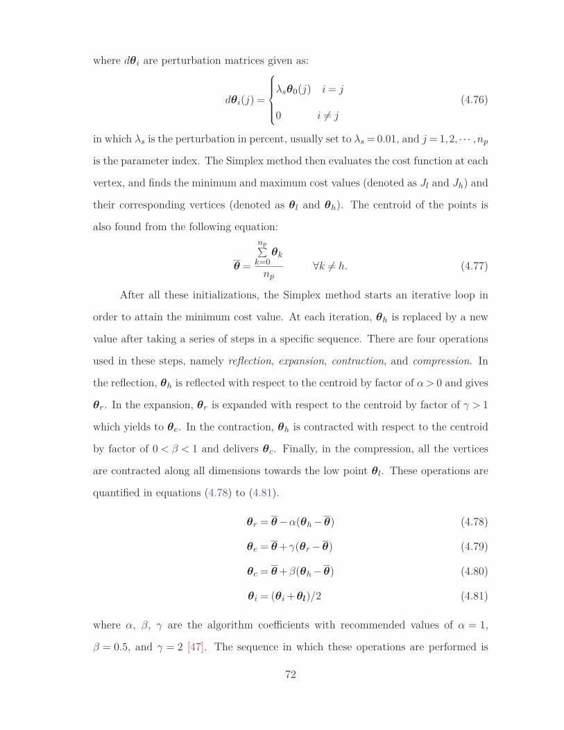
where dθi are perturbation matrices given as:
dθi(j) =
⎧⎪⎪⎪⎨⎪⎪⎪⎩
λsθ0(j) i = j
0 i �= j
(4.76)
in which λs is the perturbation in percent, usually set to λs = 0.01, and j = 1,2, · · · ,np
is the parameter index. The Simplex method then evaluates the cost function at each
vertex, and finds the minimum and maximum cost values (denoted as Jl and Jh) and
their corresponding vertices (denoted as θl and θh). The centroid of the points is
also found from the following equation:
θ =
np∑k=0
θk
np∀k �= h. (4.77)
After all these initializations, the Simplex method starts an iterative loop in
order to attain the minimum cost value. At each iteration, θh is replaced by a new
value after taking a series of steps in a specific sequence. There are four operations
used in these steps, namely reflection, expansion, contraction, and compression. In
the reflection, θh is reflected with respect to the centroid by factor of α > 0 and gives
θr. In the expansion, θr is expanded with respect to the centroid by factor of γ > 1
which yields to θe. In the contraction, θh is contracted with respect to the centroid
by factor of 0 < β < 1 and delivers θc. Finally, in the compression, all the vertices
are contracted along all dimensions towards the low point θl. These operations are
quantified in equations (4.78) to (4.81).
θr = θ −α(θh −θ) (4.78)
θe = θ +γ(θr −θ) (4.79)
θc = θ +β(θh −θ) (4.80)
θi = (θi +θl)/2 (4.81)
where α, β, γ are the algorithm coefficients with recommended values of α = 1,
β = 0.5, and γ = 2 [47]. The sequence in which these operations are performed is
72

discussed with scrutiny in references [5,48]. In order to give a better understanding,
the aforementioned operations are illustrated graphically in Fig. 4.4 for a typical
three-dimensional simplex.
Figure 4.4: Possible outcomes of a step in Simplex method (adopted from [5])
At the end of the iteration, the new cost values are computed for the updated
vertices, minimum and maximum cost values are found again, and a termination or
convergence criteria is checked. The iterative loop is continued until the termination
criteria is satisfied. A typical convergence criteria requires the relative difference
between minimum and maximum cost value to be sufficiently small, that is:
∣∣∣∣Jh −Jl
Jh +Jl
∣∣∣∣ < 1.0×10⁻⁸. (4.82)
In this work, the Downhill Simplex technique is utilized in order to find the pa-
rameter estimates which minimize the cost functions of equations (4.40) and (4.42) for
short-period and roll model structures presented in Table 4.1. It is obvious that the
Simplex method has less complexity in its formulation and computation burden com-
pared to the Levenberg-Marquardt method introduced earlier.
73

4.6 Identification of the Model
The model identification problem was decreased to a nonlinear estimation problem
after postulating a proper model structure in Section 4.3.4. For the transfer func-
tions presented in Table 4.1, two nonlinear estimation problems are formulated, i.e.
OE and FE, each of which is solved by employing two nonlinear optimization rou-
tines, i.e. Levenbverg-Marquardt and Downhill Simplex. A Matlab code is generated
for this reason. The Matlab program inputs the time-history data and delivers the
identified LOES models. A schematic of the developed tool is represented in Fig. 4.5
Figure 4.5: Schematic of the parametric SID tool
Beside identifying the models using our Matlab-based SID tool, the same time-
history data are fed to CIFER NAVFIT package for identifying another set of LOES
models for comparison. Since the longitudinal and the lateral cyclic inputs are the
only controls excited using frequency sweeps during the flight test, we are only able to
identify the LOES models for short-period and roll modes. However, the Matlab code
is quite capable for identifying the heave and yaw dynamics provided that the data is
available. The Matlab package could be easily adapted for any transfer function form
as well. In this section, we will provide the estimation results for longitudinal and
lateral low order models, and compare them with the results obtained from CIFER.
74

4.6.1 Longitudinal Dynamics
The parameters to be estimated are b1, b0, a1, a0, and τ from the transfer function
given in Table 4.1. For the Levenberg solution, parameters τ and b0 are fixed during
the iterations. They are initially set to their corresponding values from CIFER,
however they are fine-tuned manually during multiple runs of the Matlab code. For
the Simplex solution, the only parameter kept fixed is time delay τ .
The results of the OE method for the short-period mode is given in Table 4.2
which includes: estimated parameters, calculated modal characteristics (ζ and ωn),
and estimation final cost value for both Levenberg and Simplex solutions. Likewise,
the FE estimation results are collected in Table 4.3, in addition to the results obtained
from CIFER. Figure 4.6 contains the pitch-rate estimates and measurements in both
frequency-domain (|q|) and time-domain (q). Also, Fig. 4.7 depicts the Bode plot
of the estimated model and measurement data, plus the time-domain verification of
the estimated pitch-rate.
Table 4.2: Identification results: OE method for short-period dynamics
SymbolsParameter Estimates
Levenberg Simplex
b1 -14.18 -10.07
b0 -400.00 -391.07
a1 12.63 9.99
a0 368.22 406.36
τ 0.08 0.08
ζ 0.33 0.25
ωn 19.19 20.16
JOE 145.79 158.38
75

Table 4.3: Identification results: FE method for short-period dynamics
SymbolsParameter Estimates
Levenberg Simplex CIFER�
b1 -25.45 -10.05 -1.18
b0 -400.00 -407.37 -566.60
a1 15.28 10.04 9.41
a0 390.19 394.15 451.69
τ 0.08 0.08 0.06
ζ 0.39 0.25 0.22
ωn 19.75 19.85 21.25
JF E 18.43 20.72 44.42
10−1 100 101 102−40−30−20−10
0
10
20
30
ω, rad/s
|q|,dB
datalevenbergsimplex
0 5 10 15 20 25 30 35 40−200−150−100−50
0
50
100
150
t, s
q,deg/s
Figure 4.6: Identification results: OE method for short-period dynamics
76

10−1 100 101 102−15−10−50
5
10
ω, rad/s
|H|,dB
dataciferlevenbergsimplex
10−1 100 101 10220406080
100120140160180200220
ω, rad/s
�H,deg
0 5 10 15 20 25 30 35 40−150−100−50
0
50
100
150
t, s
q,deg/s
Figure 4.7: Identification results: FE method for short-period dynamics
4.6.2 Lateral Dynamics
The parameters to be estimated are b0, a1, a0, and τ from the transfer function
given in Tables 4.1. For the Levenberg and Simplex solutions, only time delay τ is
fixed during the iterations. It is initially set to its corresponding value from CIFER,
but fine-tuned manually during multiple runs of the Matlab code. Analogous to the
77

longitudinal mode, Table 4.4 and 4.5 summarize the estimation results of the output-
error and frequency-response-error methods, respectively. Also, Fig. 4.9 and Fig. 4.8
illustrate the results of these two methods in time and frequency domains.
Table 4.4: Identification results: OE method for roll dynamics
SymbolsParameter Estimates
Levenberg Simplex
b0 491.00 391.40
a1 9.44 9.90
a0 436.21 380.00
τ 0.05 0.05
ζ 0.23 0.25
ωn 20.89 19.49
JOE 410.74 496.76
Table 4.5: Identification results: FE method for roll dynamics
SymbolsParameter Estimates
Levenberg Simplex CIFER�
b0 383.43 394.82 247.1
a1 6.13 9.86 9.84
a0 333.40 371.64 232.5
τ 0.07 0.05 0.01
ζ 0.17 0.26 0.32
ωn 18.26 19.27 15.25
JF E 66.72 132.86 147.73
78

10−1 100 101 102−10−50
5
10
15
20
ω, rad/s
|H|,dB
dataciferlevenbergsimplex
10−1 100 101 102−200−180−160−140−120−100−80−60−40−20
0
ω, rad/s
�H,deg
0 5 10 15 20 25 30−150−100−50
0
50
100
150
t, s
p,deg/s
Figure 4.8: Identification results: FE method for roll dynamics
4.7 Analysis and Discussion
The accuracy of the estimation can be examined by evaluating the Cramer-Rao
bound for each parameter, as given in equations (4.55) and (4.56). The Cramer-Rao
bounds for the parameters which were kept free during the optimization are given
79

10−1 100 101 102−40−30−20−10
0
10
20
ω, rad/s
|p|,dB
datalevenbergsimplex
0 5 10 15 20 25 30−150−100−50
0
50
100
150
t, s
p,deg/s
Figure 4.9: Identification results: OE method for roll dynamics
in Table 4.6 for the short-period and the roll dynamics. According to reference [12],
a highly reliable model identification with proper predictive accuracy is achieved if
the cost value and Cramer-Rao bounds agree with the following guidelines:
JF E ≤ 100 (4.83)
CRF E ≤ 40%. (4.84)
It is also worth mentioning that due to the different definitions for the cost function of
the output-error and the frequency-response-error methods (equations (4.40) and (4.42)),
the resulting cost values, JOE and JF E , are incomparable. This also involves the
Cramer-Rao bounds, CROE and CRF E , as they result from the second-order gradi-
ent of the cost function according to equation (4.54).
80

Table 4.6: Cramer-Rao bound for short-period dynamics
Mode Parameter CRF E % CROE %
Pitch
b1 36.709 0.018
a1 22.604 0.012
a0 4.046 0.032
Roll
b0 48.049 0.297
a1 52.036 0.788
a0 39.835 0.263
Overall, the identified LOES models for pitch and roll dynamics are very ac-
curate in mid and high frequencies, as can be seen in Figures 4.6 to 4.8. However,
the LOES model prediction of the low-frequency longitudinal and lateral dynamics
(lower than 0.8 rad/s for pitch, and 1 rad/s for roll motion) is relatively poor and not
acceptable. Besides, in the identified LOES models for the short-period mode using
OE and FE methods, the Levenberg solution gives a better fit with lower cost values
(see Tables 4.2 and 4.3). This is also consistent with the identified LOES models for
the roll dynamics (see Tables 4.4 and 4.5). Moreover, the LOES models for pitch
and roll dynamics obtained from OE and FE methods are superior compared to the
models identified using CIFER transfer function identification package, as they have
relatively lower cost values (see Tables 4.3 and 4.5).
From another point of view, the identified LOES model for the the longitudinal
mode is more accurate compared to the lateral model. This is consistent for all
methods and solutions, in other words:
(JF E)pitch < (JF E)roll (4.85)
(JOE)pitch < (JOE)roll (4.86)
81

(CRF Ei)pitch < (CRF Ei
)roll ∀ i = 1, · · · ,np (4.87)
(CROEi)pitch < (CROEi
)roll ∀ i = 1, · · · ,np (4.88)
where n is the number of parameters kept free during the estimation. The better
results for longitudinal identified model can be essentially seen in the simpler lon-
gitudinal dynamics compared to the lateral dynamics which is highly coupled with
directional motion. In other words, the second-order LOES model might not be suf-
ficient for capturing the lateral dynamics completely. However, the most probable
reason is the poor excitation of the roll dynamics as can be seen in spectral estimates
of the lateral input presented and discussed in Section 3.5. These results can be fur-
ther augmented if a new set of flight test data, which is richer in frequency content,
is available [49].
From another point of view, the parameter estimates reflect a physically mean-
ingful prediction of the Trex-700 longitudinal and lateral dynamics, which is in agree-
ment with the identification results of R-50 small-scale helicopter presented in refer-
ence [16]. This can be seen in the calculated modal characteristics given in Tables 4.2
to 4.5. The modal characteristics of the longitudinal dynamics (ωn = 19.75 rad/s and
ζ = 0.39) shows a fast oscillatory moderately damped short-period mode. For the lat-
eral dynamics, the modal characteristics (ωn = 18.26 rad/s and ζ = 0.17) also reflect
a relatively fast lightly damped roll mode. Among various identified model for each
mode, the FE method with Levenberg solution gives the most accurate result. The
final results for the LOES transfer functions of the longitudinal and lateral on-axis
responses are presented in the following equations:
q
δlon= −25.45s−400.00
s2 +15.28s+390.19e−0.08s (4.89)
p
δlat= 383.43
s2 +6.13s+333.40e−0.07s. (4.90)
82

Chapter 5
Conclusion
Finding an accurate mathematical model for expressing aerodynamic behavior of
small-scale aerial vehicles is a challenging task in model-based flight research. The
lack of accuracy in conventional analytical models calls for the need to use alternative
techniques for modeling these types of aircraft. System identification is considered
as a reliable and less expensive substitute approach which provides highly accurate
models in various forms, such as frequency-response, transfer function, state-space,
or nonlinear models from measured flight data.
This thesis provided an overview of frequency-domain identification approaches,
namely frequency-response and LOES methods, and their corresponding estimation
and optimization techniques. It also shed some light on flight experiment design,
and model structure determination as crucial prerequisites for a consistent model
identification. The primary purpose of this work is developing an identification tool
for rotary-wing UAVs which can automatically and efficiently interact with the flight
simulation software available for the test platforms. The developed tool can be used
as a groundwork for in-flight system identification applied to fault-tolerant and adap-
tive control. It can also optimize the control system design procedure by delivering
more realistic models.
83

A Matlab-based tool is developed throughout this research. Real flight data
have been used to verify the merit of the developed tool for identifying persistent
and reliable models. This involved designing and conducting flight test for acquiring
measurement input-output data of a test vehicle. The aircraft selected for this reason
is a flybarless single-rotor R/C helicopter named Trex-700. The flight test is executed
by MicroPilot in hover regime by exciting longitudinal and lateral cyclic controls
using frequency sweep inputs. The resulting input-output pairs for pitch and roll
motions are fed to the identification tool as well as CIFER to obtain non-parametric
and transfer function models of the aircraft. Accuracy metrics and results comparison
depict an excellent match between CIFER models and the models extracted using
the SID tool in almost entire frequency range of interest. This demonstrates the
capability of the developed system identification tool for estimating accurate models
for unmanned helicopters.
One future direction of this research can be considered as extending the cur-
rent framework to MIMO state-space model identification. This developed code can
be also used for development and application of new theory and methodologies in
system identification. Also, an important extension of this research is considered
as in-flight identification which requires employing non-iterative methods which are
also capable of state estimation, such as filter-based recursive approaches. In another
future direction, the model identified for the test vehicle can be further analyzed and
validated by conducting additional flight experiments and acquiring more measure-
ments in order to include other dynamic modes such as heave and yaw. Also, the
doublet inputs designed in Chapter 2 can be utilized in future flight test to collect
data for time-domain model validation. Finally, in the frequency-response identifica-
tion, improved spectral estimates can be achieved if a nonlinear optimization is used
for the composite windowing technique.
84

Bibliography
[1] B. Mettler, M. B. Tischler, and T. Kanade, “System identification of small-
size unmanned helicopter dynamics,” in The American Helicopter Society 55th
Forum, (Montreal, Quebec, Canada), May 1999.
[2] E. B. Stear et al., “System identification for integrated aircraft development
and flight testing,” in Proceedings of the RTO Systems Concepts and Integration
Panel (SCI) Symposium, (Madrid, Spain), 1998.
[3] L. R. Rabiner, R. W. Schafer, and C. M. Rader, “The chirp z-transform al-
gorithm and its application,” Bell System Technical Journal, vol. 48, no. 5,
pp. 1249–92.
[4] G. D. Padfield, Helicopter flight dynamics: The theory and application of flying
qualities and simulation modelling. Blackwell Publication Ltd., 2nd ed., 2007.
[5] W. H. Press, B. P. Flannery, S. A. Teukolsky, and W. T. Vetterling, Numerical
recipes in FORTRAN 77: The art of scientific computing. Cambridge University
Press, 2nd ed., 1992.
[6] J. L. Crassidis and J. L. Junkins, Optimal estimation of dynamic systems. CRC
press, 2011.
85

[7] C. R. Theodore, M. B. Tischler, and J. D. Colbourne, “Rapid frequency-domain
modeling methods for unmanned aerial vehicle flight control applications,” Jour-
nal of Aircraft, vol. 41, no. 4, pp. 735–743, 2004.
[8] P. G. Hamel and J. Kaletka, “Advances in rotorcraft system identification,”
Progress in Aerospace Sciences, vol. 33, no. 3-4, pp. 259–284, 1997.
[9] B. F. Mettler, Modeling small-scale unmanned rotorcraft for advanced flight
control design. PhD thesis, 2001.
[10] V. Klein and E. A. Morelli, Aircraft system identification: theory and practice.
American Institute of Aeronautics and Astronautics, 2006.
[11] G. Chowdhary and R. Jategaonkar, “Aerodynamic parameter estimation from
flight data applying extended and unscented kalman filter,” Aerospace Science
and Technology, vol. 14, no. 2, pp. 106–17, 2010.
[12] M. B. Tischler and R. K. Remple, Aircraft and rotorcraft system identification:
engineering methods with flight-test examples. American Institute of Aeronautics
and Astronautics, 2006.
[13] E. A. Morelli, “System identification programs for aircraft (SIDPAC),” in AIAA
Atmospheric Flight Mechanics Conference, (Monterey, CA, USA), August 2002.
[14] B. Mettler, T. Kanade, and M. B. Tischler, “System identification modeling of
a model-scale helicopter,” Tech. Rep. CMU-RI-TR-00-03, 2000.
[15] B. Mettler, M. B. Tischler, and T. Kanade, “System identification modeling
of a small-scale unmanned rotorcraft for flight control design,” Journal of the
American Helicopter Society, vol. 47, no. 1, pp. 50–63.
[16] B. Mettler, Identification modeling and characteristics of miniature rotorcraft.
Kluwer Academic Publishers, 2003.
86

[17] G. Cai, B. M. Chen, K. Peng, M. Dong, and T. H. Lee, “Modeling and control
system design for a UAV helicopter,” in Proceedings of the 14th Mediterranean
Conference on Control and Automation, (Piscataway, NJ, USA), June 2006.
[18] J. Grauer, J. Conroy, J. H. J., J. Humbert, and D. Pines, “System identification
of a miniature helicopter,” Journal of Aircraft, vol. 46, no. 4, pp. 1260–1269,
2009.
[19] J. K. Conroy, J. S. Humbert, and D. J. Pines, “Technical note: System identi-
fication of a rotary-wing micro air vehicle,” Journal of the American Helicopter
Society, vol. 56, no. 2, p. 25001, 2011.
[20] W. Yuan and J. Katupitiya, “A two-stage method for the parametric identifica-
tion of scale-model helicopter dynamics,” in AIAA Atmospheric Flight Mechan-
ics Conference, (Minneapolis, MN, USA), August 2012.
[21] E. R. Ulrich, J. S. Humbert, and D. J. Pines, “Pitch and heave control of robotic
Samara micro air vehicles,” Journal of Aircraft, vol. 47, no. 4, pp. 1290–9, 2010.
[22] S. Kim and D. Tilbury, “Mathematical modeling and experimental identification
of an unmanned helicopter robot with flybar dynamics,” Journal of Robotic
Systems, vol. 21, no. 3, pp. 95–116.
[23] A. Al-Radaideh, A. A. Jhemi, and M. Al-Jarrah, “System identification of the
Joker-3 unmanned helicopter,” in AIAA Modeling and Simulation Technologies
Conference, (Minneapolis, MN, USA), August 2012.
[24] G. Cai, B. M. Chen, K. Peng, M. Dong, and T. H. Lee, “Modeling and con-
trol of the yaw channel of a UAV helicopter,” IEEE Transactions on Industrial
Electronics, vol. 55, no. 9, pp. 3426–34, 2008.
[25] R. V. Jategaonkar, “Flight vehicle system identification in time domain: Short
course (tutorial) notes,” Tech. Rep. NASA-TM-89428, 2009.
87

[26] A. Wypyszynski, “Flight testing of small remotely piloted aircraft for system
identification,” Master’s thesis, 2009.
[27] J. N. Williams, J. A. Ham, and M. B. Tishler, “Flight test manual: rotorcraft
frequency domain flight testing,” Tech. Rep. 93-14, 1995.
[28] R. Jategaonkar, Flight vehicle system identification: A time domain methodol-
ogy. American Institute of Aeronautics and Astronautics, 2006.
[29] E. A. Morelli, “Low-order equivalent system identification for the Tu-144LL
supersonic transport aircraft,” Journal of Guidance, Control, and Dynamics,
vol. 26, no. 2, pp. 354–362, 2003.
[30] E. A. Morelli, “Identification of low order equivalent system models from flight
test data,” Tech. Rep. 210117, 2000.
[31] Align Corporation Limited, Taiwan, Trex-700E Instruction Manual, 2012.
[32] C. M. Close, D. K. Frederick, and J. C. Newell, Modeling and analysis of dynamic
systems. Wiley, 3rd ed., 2002.
[33] E. Morelli, “High accuracy evaluation of the finite fourier transform using sam-
pled data,” Tech. Rep. NASA-TM-110340, 1997.
[34] J. S. Bendat and A. G. Piersol, Random data: Analysis and measurement pro-
cedures. Wiley, 4th ed., 2010.
[35] J. Antoni and J. Schoukens, “FRF measurements with the weighted overlapped
segment averaging technique,” in IFAC Symposium Modelling, Identification and
Signal Processing (SYSID 2006) Identification and System Parameter Estima-
tion, (Amsterdam, Netherlands), 2006.
[36] A. Bramwell, G. Done, and D. Balmford, Bramwell’s Helicopter Dynamics.
American Institute of Aeronautics and Astronautics, 2001.
88

[37] W. Johnson, Helicopter Theory. Dover Publications, 1994.
[38] A. Dorobantu, Test Platforms for Model-Based Flight Research. PhD thesis,
2013.
[39] M. B. Tischler and M. G. Cauffman, “Frequency-response method for rotorcraft
system identification: Flight applications to BO 105 coupled rotor/fuselage dy-
namics,” Journal of the American Helicopter Society, vol. 37, no. 3, pp. 3–17.
[40] R. Nelson, Flight stability and automatic control. McGraw-Hill, 1998.
[41] W. Duncan, Principles of Control and Stability of Aircraft. Cambridge Univer-
sity Press, 2003.
[42] I. A. Raptis, Linear and nonlinear control of unmanned rotorcraft. PhD thesis,
2010.
[43] Y. Ben, Development of a miniature low-cost UAV helicopter autopilot platform
and formation flight control of UAV teams. PhD thesis, 2010.
[44] S. Bhandari, Flight validated high-order models of UAV helicopter dynamics in
hover and forward flight using analytical and parameter identification techniques.
PhD thesis, 2007.
[45] R. L. W. Choi, C. E. Hann, and X. Chen, “Minimal models to capture the dy-
namics of a rotary unmanned aerial vehicle,” Journal of Intelligent and Robotic
Systems: Theory and Applications, pp. 1–25.
[46] J. Wright and J. Cooper, Introduction to Aircraft Aeroelasticity and Loads. Wi-
ley, 2008.
[47] T. Takahama and S. Sakai, “Constrained optimization by applying the α con-
strained method to the nonlinear simplex method with mutations,” IEEE Trans-
actions on Evolutionary Computation, vol. 9, no. 5, pp. 437–451.
89

[48] J. A. Nelder and R. Mead, “A Simplex method for function minimization,” The
Computer Journal, vol. 7, no. 4, pp. 308–313.
[49] M. Mohajerani, H. Bolandhemmat, Y. Zhang, and H. Loewen, “Identification
of low order equivalent transfer function model of Trex-700E helicopter from
flight test data,” in AIAA Modeling and Simulation Technologies Conference,
(Reston, VA, USA), 2014.
90