FREQUENCY DOMAIN SYSTEM IDENTIFICATION AND IT’S APPLICATION IN JAMMING

A THESIS SUBMITTED IN THE PARTIAL FULFILLMENT

OF THE REQUIREMENTS FOR THE DEGREE OF

Bachelor of Technology

In

Electronics and Communication

by

ARNAB MANDAL

Roll No: 110EC0170

Department of Electronics & Communication Engineering

National Institute of Technology

Rourkela

FREQUENCY DOMAIN SYSTEM IDENTIFICATION AND IT’S APPLICATION IN JAMMING

A THESIS SUBMITTED IN PARTIAL FULFILLMENT

OF THE REQUIREMENTS FOR THE DEGREE OF

Bachelor of Technology

In

Electronics and Communication

by

ARNAB MANDAL

Roll No: 110EC0170

Under the guidance of

Prof. A.K SAHOO

Department of Electronics & Communication Engineering

National Institute of Technology

Rourkela

National Institute Of Technology Rourkela

CERTIFICATE

This is to certify that the thesis entitled, “FREQUENCY DOMAIN SYSTEM

IDENTIFICATION AND IT’S APPLICATION IN JAMMING” submitted by ARNAB

MANDAL in partial fulfilment of the requirements for the award of Bachelor of

Technology degree in Electronics and Communication Engineering during

session 2010-2014 at National Institute of Technology, Rourkela (Deemed

University) is an authentic work by him under my supervision and guidance.

Date: Prof. A.KSAHOO

Dept. of ECE National Institute of Technology

Rourkela-769008

Email: ajitsahoo@nitrkl.ac.in

ACKNOWLEDGEMENT

I have taken efforts in this project. However, it would not have been possible without the kind support and help of many individuals and organizations. I would like to extend my sincere thanks to all of them.

I am highly indebted to Prof.Ajit kumar Sahu for his guidance and constant supervision as well as for providing necessary information regarding the project & also for his support in completing the project. I would like to express my gratitude towards my parents & the professors of my department,

Prof. Sarat Patra, Prof. K.K. Mahapatra, Prof. Poonam Singh for their kind co-operation and encouragement which helped me in completion of this project. I would like to express my special gratitude and thanks to my friends for giving me an inspiration to complete this project in time. Last but not the least my thanks and appreciations also goes to the Phd. scholar, Sananda Kumar for his kind cooperation during the period of this assignment which finally helped me in developing this project.

Arnab Mandal 110ec0170

rik.mandal92@gmail.com

ABSTRACT:

Identification is a powerful technique used to build accurate models of system from noisy data. The Frequency Domain System Identification utilizes specialized tools for identifying linear dynamic multiple input/single-output (MISO) systems from time responses or measurements of the system's frequency response. Frequency domain methods supports continuous-time modeling, which can be a powerful and highly accurate complement to the more commonly used discrete-time methods. The methods described here can be applied to problems such as the modeling of electronic, mechanical, and acoustical systems. A brief intuitive introduction to system identification using adaptive filters has been provided.

Adaptive filtering has been broadly divided into seven broad categories .The first part describes linear and non-linear filtering and gives an overview of various kinds of estimation techniques. The second part describes Weiner filter and its applications in real world. The third part introduces system modeling like stochastic and stationary models. In the fourth part we describe the least mean square algorithm and it’s error performance. The fifth part gives an overview of variants of LMS like sign LMS, block LMS, normalized LMS. The sixth part introduces transform domain adaptive filtering and algorithms used like DCT/DFT LMS. The last part is an implementation of system identification in design of a jam resistant receiver.

CHAPTER 1

Introduction

An adaptive filter is a system with a linear filter that has a transfer function controlled by

variable parameters and a means to adjust those parameters according to an optimization The

Frequency Domain System Identification Toolbox (FDIDENT) provides specialized tools for

identifying linear dynamic single-input/single-output (SISO) systems from time responses or

measurements of the system's frequency response. Frequency domain methods support

continuous-time modeling, which can be a powerful and highly accurate complement to the

more commonly used discrete-time methods. The methods in the toolbox can be applied to

problems such as the modeling of electronic, mechanical, and acoustical systems algorithm.

Because of the complexity of the optimization algorithms, most adaptive filters are digital

filters. Adaptive filters are required for some applications because some parameters of the

desired processing operation (for instance, the locations of reflective surfaces in a reverbing

space) are not known in advance or are changing. The closed loop adaptive filter uses feedback

in the form of an error signal to refine its transfer function.

The term filter is ordinarily used to allude to a framework that is intended to concentrate data

around a recommended amount of enthusiasm from uproarious data. With such expansive

point estimation hypothesis discovers provisions in numerous various fields: correspondence,

radar, route, biomedical engg.

THE THREE BASIC KINDS OF ESTIMATION

1.FILTERING:It is an operation that involves extraction of information about a quantity of

interest at time t by using data measured up to and including time t.

2.SMOOTING:It is an a posteriori form of estimation, in that data measured after the time of

interest are used in estimation. The smoothed estimate a t time t’ is obtained by using data

measured over the interval [0,t],where t’<t. A delay of t-t’ is therefore introduced in computing

the smoothed estimate .The benefit gained is that by waiting for more data to accumulate, a

more accurate estimate can be found.

3.PREDICTION: The forecasting side of estimation, with aim to derive information about the

quantity of interest will be like at future time (t+t1)where t1>0,by using data measured upto

and including time t.

LINEAR VS NONLINEAR FILTERING

In signal processing, a nonlinear (or non-linear) filter is a filter whose yield is not a linear

function of its input. That is, if the filter outputs signals R and S for two input

signals rand s separately, yet does not generally yield αR + βS when the input is a linear

combination αr + βs.

Both continuous-domain and discrete-domain filters may be nonlinear. A straightforward case

of the previous might be an electrical gadget whose yield voltage R(t) at any moment is the

square of the data voltage r(t); or which is the information cut to an altered extent [a,b],

specifically R(t) = max(a, min(b, r(t))). An essential sample of the recent is the running-median

filter , such that each yield test Ri is the average of the last three data tests ri, ri−1, ri−2. An

important example of the latter is the running-median filter , such that every output

sample Ri is the median of the last three input samples ri, ri−1, ri−2. Like linear filters, nonlinear

filters may be shift invariant or not.

Non-linear filters have numerous requisitions,, especially in the removal of certain types

of noise that are not additive. For instance, the median filter is widely used to remove spike

noise — that influences just a little rate of the specimens,, possibly by very large amounts.

Indeed all radio receivers utilize non-linear filters to convert kilo- to gigahertz signals to

the audio frequency range; and all digital signal processing depends on non-linear filters

(analog-to-digital converters) to transform analog signals to binary numbers.

Then again, nonlinear filters are significantly harder to utilize and outline than linear ones, on

the grounds that the most compelling numerical devices of sign examination, (for example, the

motivation reaction and the recurrence reaction) can't be utilized on them. Thus, for example,

linear filters are often used to remove noise and distortion that was created by nonlinear

processes, simply because the proper non-linear filter would be too hard to design and construct.

Linear filters process time-varying input signals to produce output signals, subject to the

requirements of linearity [2]. This results from systems made exclusively out of components (or

digital algorithms) classified as having a linear response. Most filters implemented in analog

electronics, in digital signal processing, or in mechanical systems are classified as causal, time

invariant, and linear.

The general concept of linear filtering is also used in statistics, data analysis, and mechanical

engineering among other fields and technologies [10]. This includes non-causal filters and filters

in more than one dimension such as would be used in image processing; those filters are

subject to different constraints leading to different design methods.

CHAPTER 2

2.1 WEINER FILTER

2.2 ERROR ESTIMATION

2.3 DISCRETE SERIES WEINER FILTER

2.4 APPLICATIONS

2.1 WEINER FILTER

The outline of a Weiner filter requires from the earlier data about the facts of information to be

transformed. It produces an estimate of a desired or target random process by linear time-

invariant filtering an observed noisy process, assuming known stationary signal and noise

spectra, and additive noise [6]. The Wiener filter minimizes the mean square error between the

estimated random process and the desired process.

The goal of the Wiener filter is to filter out noise that has corrupted a signal. It is based on

a statistical approach. Typical filters are designed for a desired frequency response. However,

the design of the Wiener filter takes a different approach [11]. One is expected to have learning

of the spectral properties of the original signal and the noise, and one seeks the linear time-

invariant filter whose output might verge to the original signal as possible. Wiener filters are

characterized by the following:

1. Assumption: signal and (additive) noise are stationary linear stochastic processes with

known spectral characteristics or known autocorrelation and cross-correlation

2. Requirement: the filter must be physically realizable/causal (this requirement can be

dropped, resulting in a non-causal solution)

3. Performance criterion: minimum mean-square error (MMSE)

2.2 ERROR ESTIMATION

The input to the Wiener filter is assumed to be a signal s(t), corrupted by additive noise, n(t).

The output, s^(t) is calculated by means of a filter, g(t) using the following convolution:[1]

where is the original signal (not exactly known; to be estimated), is the

noise, is the estimated signal (the intention is to equal , and is the

Wiener filter's impulse response.

The error is defined as

where is the delay of the Wiener Filter (since it is causal). In other words, the error is

the difference between the estimated signal and the true signal shifted by .

The squared error is

where is the desired output of the filter and is the error. Depending on

the value of , the problem can be described as follows:

if then the problem is that of prediction (error is reduced when is

similar to a later value of s),

if then the problem is that of filtering (error is reduced when s*(t) is

similar to , and

if then the problem is that of smoothing (error is reduced when is

similar to an earlier value of s).

.

Taking the expected value of the squared error results in

where is the observed signal, is the autocorrelation function

of , is the autocorrelation function of , and is the cross-correlation

function of and . If the signal and the noise are uncorrelated (i.e., the

cross-correlation is zero), then this means that and .

For many applications, the assumption of uncorrelated signal and noise is reasonable.

The objective is to minimize , the expected value of the squared error, by calculating

the optimal , the Wiener filter impulse response function. The minimum may be found

by finding the first order incremental change in the least square resulting from an

incremental change in for positive time. This is

For a minimum, this must vanish identically for all for which leads to

the Wiener–Hopf equation:

This is the fundamental equation of the Wiener theory. The right-hand side

resembles a convolution but is only over the semi-infinite range. The equation can

be solved to find the optimal filter by a special technique due to Wiener

and Hopf.

2.3Finite impulse response Wiener filter for discrete series

The causal finite impulse response (FIR) Wiener filter, instead of using some given data matrix X

and output vector Y, finds optimal tap weights by making use of the statistics of the input and

output signals. It populates the data network X with estimates of the auto-correlation of the

input signal (T) and populates the output vector Y with estimates of the cross-correlation

between the output and input signals (V).

In order to derive the coefficients of the Wiener filter, consider the signal w[n] being fed to a

Wiener filter of order N and with coefficients , . The output of the filter

is denoted x[n] which is given by the expression

The residual error is denoted e[n] and is defined as e[n] = x[n] − s[n] (see the corresponding

block diagram). The Wiener channel is outlined in order to minimize the mean square slip

(MMSE criteria) which might be expressed compactly:

where denotes the expectation operator. In the general case, the

coefficients may be complex and may be derived for the case where w[n] and s[n]

are complex as well. With a complex signal, the matrix to be solved is

a Hermitian Toeplitz matrix, rather than symmetric Toeplitz matrix[17]. For simplicity,

the following considers only the case where all these quantities are real. The mean

square error (MSE) may be rewritten as:

To find the vector which minimizes the expression above, calculate

its derivative with respect to

Assuming that w[n] and s[n] are each stationary and jointly stationary, the

sequences and known respectively as the autocorrelation

of w[n] and the cross-correlation between w[n] and s[n] can be defined as

follows:

The derivative of the MSE may therefore be rewritten as (notice

that )

Letting the derivative be equal to zero results in

which can be rewritten in matrix form

These equations are known as the Wiener–Hopf equations. The matrix T appearing in the

equation is a symmetric Toeplitz matrix. Under suitable conditions on , these matrices are

known to be positive definite and therefore non-singular yielding a unique solution to the

determination of the Wiener filter coefficient vector, .

The realization of the causal Wiener filter looks a lot like the solution to the least

squares estimate, except in the signal processing domain. The least squares solution, for input

matrix and output vector is

The FIR Wiener filter is related to the least mean squares filter, but minimizing the error

criterion of the latter does not rely on cross-correlations or auto-correlations. Its solution

converges to the Wiener filter solution.

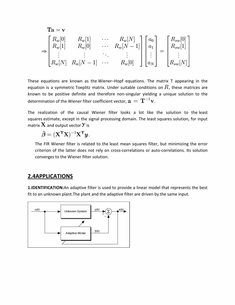
2.4APPLICATIONS

1.IDENTIFICATION:An adaptive filter is used to provide a linear model that represents the best

fit to an unknown plant.The plant and the adaptive filter are driven by the same input.

2.INVERSE MODELING: the inverse model has a transfer function that is inverse of the plant

transfer function such that the combination of the two constitutes an ideal transmission

medium.

3.PREDICTION: The present value of a random signal serves purpose of a desired response for

the filter. Past values supply the input applied to the filter.Targetis to provide best prediction of

the present value.

CHAPTER 3

3.1 STOCKHASTIC PROCESS AND MODELS

3.2 STATIONARY PROCESS

3.1STOCKHASTIC PROCESS AND MODELS

In likelihood hypothesis, a stochastic procedure or now and then random process (generally

used) is an accumulation of arbitrary qualities; this is regularly used to speak to the

advancement of some arbitrary variable, or framework, about whether. This is the probabilistic

partner to a deterministic methodology (or deterministic framework)[11]. As opposed to

portraying a methodology which can just develop in restricted (as in the case, for instance, of

results of a standard differential comparison), in a stochastic or arbitrary process there is some

indeterminacy: regardless of the fact that the introductory condition (or beginning stage) is

known, there are a few (regularly endlessly a lot of people) headings in which the procedure

might evolve.

Given a probability space and a measurable space , an S-valued stochastic

process is a collection of S-valued random variables on , indexed by a totally

ordered set T ("time"). That is, a stochastic process X is a collection

where each is an S-valued random variable on . The space S is then called the state

space of the process.

Let X be an S-valued stochastic process. For every finite sequence ,

the k-tuple is a random variable taking values in . The

distribution of this random variable is a probability measure on .

This is called a finite-dimensional distribution of X.

Under suitable topological restrictions, a suitably "consistent" collection of finite-dimensional

distributions can be used to define a stochastic process (see Kolmogorov extension in the

"Construction" section).

In econometrics and signal processing, a stochastic process is said to be ergodic if its statistical

properties (such as its mean and variance) can be deduced from a single, sufficiently long

sample (realization) of the process.[14]

the ergodicity of various properties of a stochastic process. For example, a wide-sense

stationary process has mean and

autocovariance which do not

change with time. One way to estimate the mean is to perform a time average:

If converges in squared mean to as , then the process is said to

be mean-ergodic[1] or mean-square ergodic in the first moment.

Likewise, one can estimate the autocovariance by performing a time average:

If this expression converges in squared mean to the true

autocovariance , then the

process is said to be autocovariance-ergodic or mean-square ergodic in the second moment.

A process which is ergodic in the first and second moments is sometimes called ergodic in the

wide sense.

An important example of an ergodic processes is the stationary Gaussian process with

continuous spectrum.

3.2 STATIONARY PROCESS

In statistics,a stationary methodology (or strictly) stationary procedure (or determinedly)

stationary procedure is a stochastic procedure whose joint likelihood distribution(pdf) does not

change when moved in time. Thusly, parameters, for example, the mean and change, in the

event that they are available, likewise don't change about whether and don't take after any

patterns.

Formally, let be a stochastic process and let represent

the cumulative distribution function of the joint distribution of at

times . Then, is said to be stationary if, for all , for all , and for

all ,

Since does not affect , is not a function of time.

A weaker form of stationarity commonly employed in signal processing is known as weak-sense

stationarity, wide-sense stationarity (WSS), covariance stationarity, or second-order

stationarity. WSS random processes only require that 1st moment and covariance do not vary

with respect to time. Any strictly stationary process which has amean and a covariance is also

WSS.

So, a continuous-time random process x(t) which is WSS has the following restrictions on its

mean function

and autocovariance function

The first property implies that the mean function mx(t) must be constant. The second property

implies that the covariance function depends only on the difference between and and

only needs to be indexed by one variable rather than two variables.

CHAPTER 4

4.1LEAST MEAN SQUARE ALGORITHM

4.2SYMBOL DEFINITION

4.3PROBLEM FORMULATION AND MATLAB CODE

4.4ERROR PERFORMANCE SURFACE

4.1 LEAST MEAN SQUARE ALGORITHM

The Adaptive Linear Combiner

ek = dk - XTW

ek2 = dk

2 + WTXkXkTW - 2dkXk

TW E[ek

2] = E[dk2] + WTE[XkXk

T]W - 2E[dkXkT]W

Let R = E[XkXkT] and P = e[dkXk

T] MSE = E[ek

2] = E[dk2] + WTRW - 2PTW

Least mean squares (LMS) algorithms are a class of adaptive filter used to mimic a desired filter

by finding the filter coefficients that relate to producing the least mean squares of the error

signal (difference between the desired and the actual signal). It is a stochastic gradient

descent method in that the filter is only adapted based on the error at the current time. It was

invented in 1960 by Stanford University professor Bernard Widrow and his first Ph.D.

student, Ted Hoff.

The realization of the causal Wiener filter looks a lot like the solution to the least squares

estimate, except in the signal processing domain. The least squares solution, for input

matrix and output vector is

The FIR least mean squares filter is related to the Wiener filter, but minimizing the error

criterion of the former does not rely on cross-correlations or auto-correlations. Its solution

converges to the Wiener filter solution[19]. Most linear adaptive filtering problems can be

formulated using the block diagram above. That is, an unknown system is to be identified

and the adaptive filter attempts to adapt the filter to make it as close as possible

to , while using only observable signals , and ; but

, and are not directly observable. Its solution is closely related to the Wiener filter.

4.2 Definition of symbols

is the number of the current input sample

is the filter order

(Hermitian transpose or conjugate transpose)

estimated filter; interpret as the estimation of the filter coefficients

after n samples

4.3PROBLEM FORMULATION

Example:- The One-step Predictor

R = E [ Xk XkT ]

P = E [ dk XkT ]

Now:

Using the fact that

sin2 A = 0.5(1 - cos2A) sinA sinB = 0.5[cos(A - B) - cos(A + B)] we can determine that:

Thus we can calculate R:

Now

P = E [ dk XkT ]

therefore: P = E [ dkxk-1 dkxk-2 ]T = [ xkxk-1 xkxk-2 ]T

Therefore we have:

The optimal weight vector, W* is :

W* = R-1 P =

= [ 1.6197 -1.0 ]T

CHECK THROUGH MATLAB

clc; clear all; close all;% This script implements the LMS algorithm for the sine predictor problem. x = sin((0:1000)*pi/5); w = [4;0.05]; % Initial weights

mu = 0.2; % Adaptation gain W1=[]; for k = 3:100, Xvec = [x(k-1);x(k-2)]; d(k) = x(k); y(k) = w'*Xvec; e(k) = d(k) - y(k); w = w+ 2*mu*e(k)*Xvec; W1=[W1;w]; end hold on; W1 e=e(3:100); e.^2; plot(e.^2); OUTPUT: w = 1.6233 -1.0055 Error curve

0 10 20 30 40 50 60 70 80 90 1000

1

2

3

4

5

6

7

err

or

curv

e

4.4 ERROR PERFORMANCE SURFACE

clc clear all; close all;; n = 10; m = 0; w0 = -3:0.5:3; w1 = -4:0.5:0; [X,Y]=meshgrid(w0,w1); mse = 0.5*(X.^2+Y.^2)+X.*Y*cos(2*pi/5)+2*Y*sin(2*pi/5)+2; Z=[mse]; surf(X,Y,Z) xlabel('Weight 1') ylabel('Weight 2') zlabel('Mean Square Error') view(45+n,10+m); OUTPUT:

-4-2

02

4 -4-3

-2-1

0

0

2

4

6

8

10

12

Weight 2Weight 1

Mean S

quare

Err

or

CHAPTER 5 5.1 SIGN LMS

5.2 NLMS

5.3 COMPARISON OF LMS, NLMS and SLMS

COMPARISON OF LMS, SIGN LMS and NLMS 5.1 SIGN LMS Some adaptive filter applications require you to implement adaptive filter algorithms on hardware targets, such as digital signal processing (DSP) devices, FPGA targets, and application-specific integrated circuits (ASICs). These targets require a simplified version of the standard LMS algorithm. The sign function, as defined by the following equation, can simplify the standard LMS.

algorithm.

Applying the sign function to the standard LMS algorithm returns the following three types of sign LMS algorithms.

Sign-error LMS algorithm—Applies the sign function to the error signal e(n). This algorithm updates the coefficients of an adaptive filter using the following equation: . Notice that when e(n) is zero, this algorithm does not involve multiplication operations. When e(n) is not zero, this algorithm involves only one multiplication operation.

Sign-data LMS algorithm—Applies the sign function to the input signal vector . This algorithm updates the coefficients of an adaptive filter using the following equation: . Notice that when is zero, this algorithm does not involve multiplication operations. When is not zero, this algorithm involves only one multiplication operation.

Sign-sign LMS algorithm—Applies the sign function to both e(n) and . This algorithm updates the coefficients of an adaptive filter using the following equation: . Notice that when either e(n) or is zero, this algorithm does not involve multiplication operations. When neither e(n) or is

zero, this algorithm involves only one multiplication operation.

The sign LMS algorithms involve fewer multiplication operations than other algorithms. When the step size μ equals a power of 2, the sign LMS algorithms can replace the multiplication operations with shift operations[14]. In this situation, these algorithms have only shift and addition operations. Compared to the standard LMS algorithm, the sign LMS algorithm has a slower convergence speed and a greater steady state error.

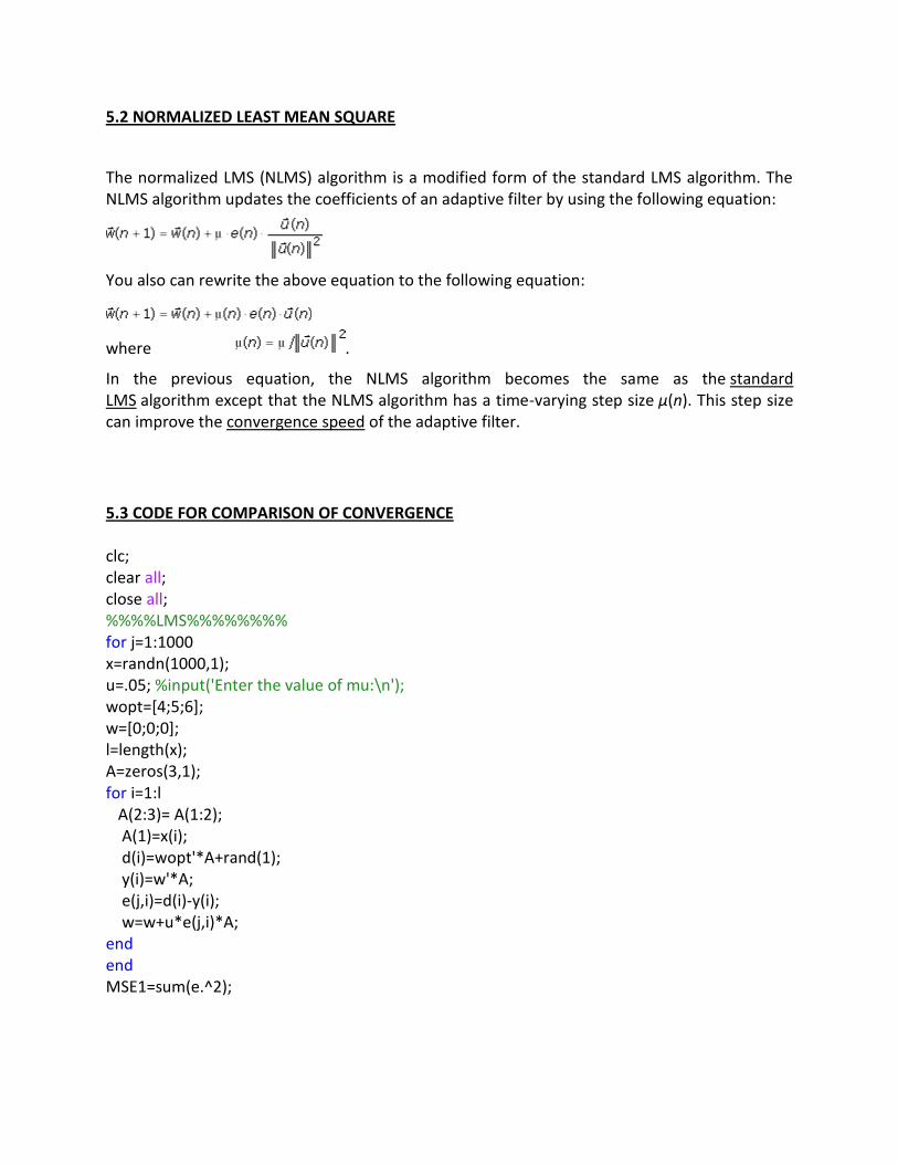
5.2 NORMALIZED LEAST MEAN SQUARE

The normalized LMS (NLMS) algorithm is a modified form of the standard LMS algorithm. The NLMS algorithm updates the coefficients of an adaptive filter by using the following equation:

You also can rewrite the above equation to the following equation:

where .

In the previous equation, the NLMS algorithm becomes the same as the standard LMS algorithm except that the NLMS algorithm has a time-varying step size μ(n). This step size can improve the convergence speed of the adaptive filter.

5.3 CODE FOR COMPARISON OF CONVERGENCE clc; clear all; close all; %%%%LMS%%%%%%%% for j=1:1000 x=randn(1000,1); u=.05; %input('Enter the value of mu:\n'); wopt=[4;5;6]; w=[0;0;0]; l=length(x); A=zeros(3,1); for i=1:l A(2:3)= A(1:2); A(1)=x(i); d(i)=wopt'*A+rand(1); y(i)=w'*A; e(j,i)=d(i)-y(i); w=w+u*e(j,i)*A; end end MSE1=sum(e.^2);

%%%%NLMS%%%%%%%% for j=1:1000 x=randn(1000,1); un=.1; %input('Enter the value of mu:\n'); wopt=[4;5;6]; w=[0;0;0]; l=length(x); A=zeros(3,1); dn=.0001; for i=1:l A(2:3)= A(1:2); A(1)=x(1); xn=A(1)^2+A(2)^2+A(3)^2; d(i)=wopt'*A+rand(1); y(i)=w'*A; e(j,i)=d(i)-y(i); w=w+(un/(dn+xn))*e(j,i)*A; end end MSE2=sum(e.^2); %%%%SLMS%%%%%%%% for j=1:1000 x=randn(1000,1); us=.05; %input('Enter the value of mu:\n'); wopt=[4;5;6]; w=[0;0;0]; l=length(x); A=zeros(3,1); dn=.0001; for i=1:l A(2:3)= A(1:2); A(1)=x(1); d(i)=wopt'*A+rand(1); y(i)=w'*A; e(j,i)=d(i)-y(i); w=w+(us)*sign(e(j,i))*A; end end MSE3=sum(e.^2); plot(MSE1,'-b');hold on; plot(MSE2,'--r');hold on;

plot(MSE3,'.-g'); leg=legend('LMS','Nlms','SLMS'); OUTPUT:

It is shown that the normalized least mean square (NLMS) algorithm is a potentially faster

converging algorithm compared to the LMS and SLMS algorithm where the design of the

adaptive filter is based on the usually quite limited knowledge of its input signal statistics.

In summary, we have described a statistical analysis of the LMS adaptive filter, and through this analysis, suggestions for selecting the design parameters for this system have been provided. While useful, analytical studies of the LMS adaptive filter are but one part of the system design process. As in all design problems, sound engineering judgment, careful analytical studies, computer simulations,and extensive real-world evaluations and testing should be combined when developing an adaptive filtering solution to any particular task.

5.4 BLOCK LMS The Block LMS Filter block implements an adaptive least mean-square (LMS) filter, where the adaptation of filter weights occurs once for every block of samples. The block estimates the filter weights, or coefficients, needed to minimize the error, e(n), between the output signal, y(n), and the desired signal, d(n).[17] Connect the signal you want to filter to the Input port. The input signal can be a scalar or a column vector. Connect the signal you want to model to the Desired port. The desired signal must have the same data type, complexity, and

0 100 200 300 400 500 600 700 800 900 10000

0.5

1

1.5

2

2.5x 10

5

LMS

Nlms

SLMS

dimensions as the input signal. The Output port outputs the filtered input signal. The Error port outputs the result of subtracting the output signal from the desired signal. The block calculates the filter weights using the Block LMS adaptive filter algorithm. This algorithm is defined by the following equations.

The weight update function for the Block LMS adaptive filter algorithm is defined as

The variables are as follows.

Variable Description

n The current time index

i The iteration variable in each block,

k The block number

N The block size

u(n) The vector of buffered input samples at step n

w(n) The vector of filter-tap estimates at step n

y(n) The filtered output at step n

e(n) The estimation error at time n

d(n) The desired response at time n

μ The adaptation step size

Use the Filter length parameter to specify the length of the filter weights vector. The Block size parameter determines how many samples of the input signal are acquired before the filter weights are updated. The number of rows in the input must be an integer multiple of the Block size parameter. The adaptation Step-size (mu) parameter corresponds to µ in the equations. You can either specify a step-size using the input port, Step-size, or enter a value in the Block Parameters: Block LMS Filter dialog box.

Use the Leakage factor (0 to 1) parameter to specify the leakage factor, , in the leaky LMS algorithm shown below.

Enter the initial filter weights as a vector or a scalar in the Initial value of filter weights text box. When you enter a scalar, the block uses the scalar value to create a vector of filter weights. This vector has length equal to the filter length and all of its values are equal to the scalar value When you select the Adapt port check box, an Adapt port appears on the block. When the input to this port is greater than zero, the block continuously updates the filter weights. When the input to this port is zero, the filter weights remain at their current values. When you want to reset the value of the filter weights to their initial values, use the Reset input parameter. The block resets the filter weights whenever a reset event is detected at the Reset port. The reset signal rate must be the same rate as the data signal input. From the Reset input list, select None to disable the Reset port. To enable the Reset port, select one of the following from the Reset input list:

Rising edge — Triggers a reset operation when the Reset input does one of the following: o Rises from a negative value to a positive value or zero

o Rises from zero to a positive value, where the rise is not a continuation of a rise from a negative value to zero (see the following figure).

Falling edge — Triggers a reset operation when the Reset input does one of the following: o Falls from a positive value to a negative value or zero

o Falls from zero to a negative value, where the fall is not a continuation of a fall from a positive value to zero (see the following figure)

Either edge — Triggers a reset operation when the Reset input is a Rising edge or Falling edge (as described above)

Non-zero sample — Triggers a reset operation at each sample time that the Reset input is not zero Select the Output filter weights check box to create a weights port on the block. For each iteration, the block outputs the current updated filter weights from this port. MATLAB CODE clc; clear all; close all; clf; size1=1000; iter=200; blk_size=8; muu=0.05; w_sys=[8 4 6 5]';l=length(w_sys); w1=zeros(l,iter); for it=1:iter x=randn(1,size1); %n=randn(1,size1);%noise w=zeros(l,1); u=zeros(1,l);%regressor vector temp=zeros(1,l); for i=1:(size1/blk_size)-1%block number is i temp=zeros(1,l); for r=0:blk_size-1 u(1,l-2:l)=u(1,1:l-1);%2:4=1:3 u(1,1)=x(i*blk_size+r); desired(i*blk_size+r)=u*w_sys+randn(1,1); %noise added estimate(i*blk_size+r)=u*w; err(it,i*blk_size+r)=desired(i*blk_size+r)-estimate(i*blk_size+r); temp=temp+err(it,i*blk_size+r).*u; end w=w+muu.*temp';%(muu'/blk_size)=muu end w1(:,it)=w; clc; fprintf('current iteration is %d ',it); end w=mean(w1,2); err_sqr=err.^2;

err_mean=mean(err_sqr,1); err_max=err_mean./max(err_mean); err_dB=10*log10(err_max); plot(err_dB); title('BLOCK LMS Algorithm'); ylabel('Mean Square Error'); xlabel('No of Iterations'); w_sys w

OUTPUT:

0 100 200 300 400 500 600 700 800 900 1000-25

-20

-15

-10

-5

0BLOCK LMS Algorithm

Mean S

quare

Err

or

No of Iterations

CHAPTER 6

6.1TRANSFORM DOMAIN ADAPTIVE FILTERS

6.2UNITARY TRANSFORMATIONS

6.3DFT LMS

6.4DCT LMS

6.1TRANSFORM DOMAIN ADAPTIVE FILTERS

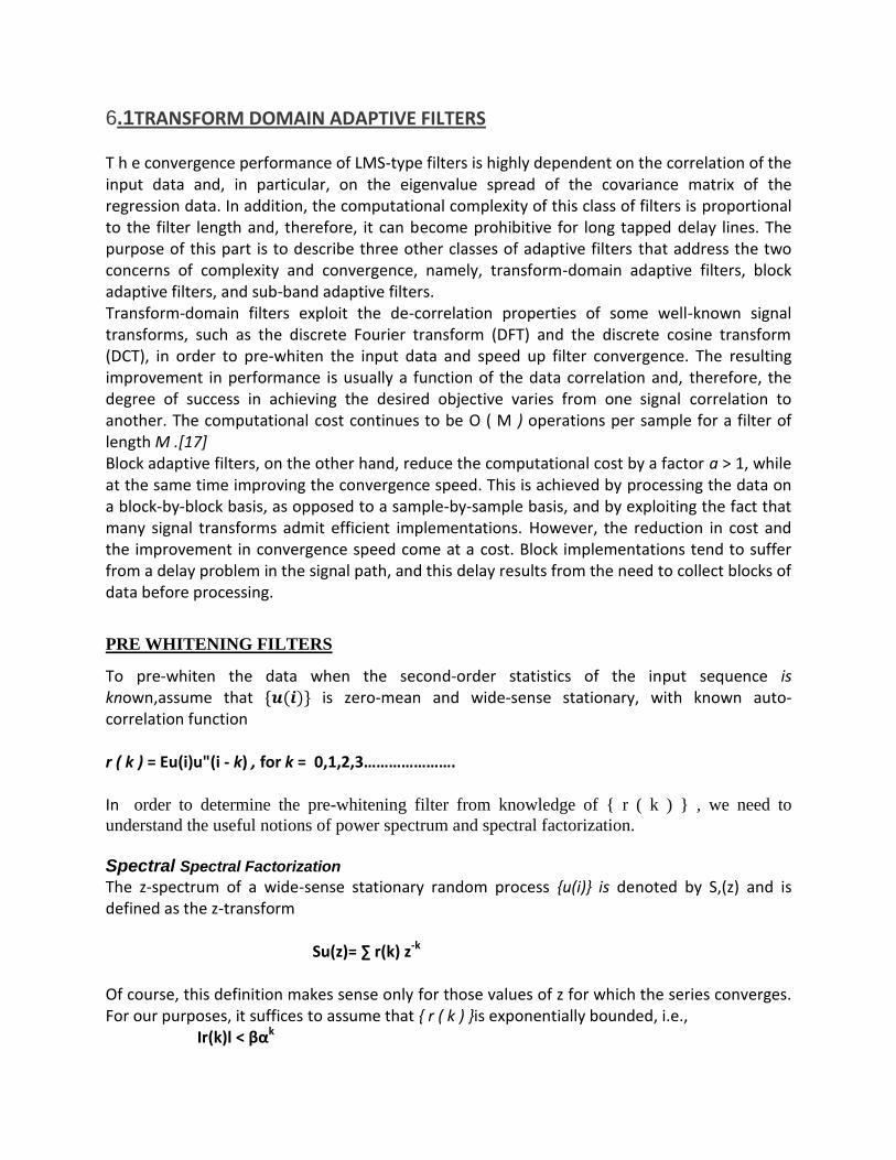
T h e convergence performance of LMS-type filters is highly dependent on the correlation of the input data and, in particular, on the eigenvalue spread of the covariance matrix of the regression data. In addition, the computational complexity of this class of filters is proportional to the filter length and, therefore, it can become prohibitive for long tapped delay lines. The purpose of this part is to describe three other classes of adaptive filters that address the two concerns of complexity and convergence, namely, transform-domain adaptive filters, block adaptive filters, and sub-band adaptive filters. Transform-domain filters exploit the de-correlation properties of some well-known signal transforms, such as the discrete Fourier transform (DFT) and the discrete cosine transform (DCT), in order to pre-whiten the input data and speed up filter convergence. The resulting improvement in performance is usually a function of the data correlation and, therefore, the degree of success in achieving the desired objective varies from one signal correlation to another. The computational cost continues to be O ( M ) operations per sample for a filter of length M .[17] Block adaptive filters, on the other hand, reduce the computational cost by a factor a > 1, while at the same time improving the convergence speed. This is achieved by processing the data on a block-by-block basis, as opposed to a sample-by-sample basis, and by exploiting the fact that many signal transforms admit efficient implementations. However, the reduction in cost and the improvement in convergence speed come at a cost. Block implementations tend to suffer from a delay problem in the signal path, and this delay results from the need to collect blocks of data before processing.

PRE WHITENING FILTERS

To pre-whiten the data when the second-order statistics of the input sequence is known,assume that is zero-mean and wide-sense stationary, with known auto-correlation function r ( k ) = Eu(i)u"(i - k) , for k = 0,1,2,3…………………. In order to determine the pre-whitening filter from knowledge of r ( k ) , we need to

understand the useful notions of power spectrum and spectral factorization.

Spectral Spectral Factorization

The z-spectrum of a wide-sense stationary random process u(i) is denoted by S,(z) and is defined as the z-transform Su(z)= ∑ r(k) z-k

Of course, this definition makes sense only for those values of z for which the series converges. For our purposes, it suffices to assume that r ( k ) is exponentially bounded, i.e., Ir(k)l < βαk

for some ,β> 0 and 0 < α < 1. In this case the series is absolutely convergent for all values of z in the annulus a < IzI < a-1, i.e., it satisfies ∑ |r(k)| |z-k

for all a < I Z I< l / a

We then say that the interval a < < a-1 defines the region of convergence (ROC) of Su(z).

Since this ROC includes the unit circle, we establish that S,(z) cannot have poles on the unit circle. Evaluating Su(z) on the unit circle then leads to what is called the power spectrum (or the power-spectral-density function) of the random process. The power spectrum has two important properties: 1.Hermitian symmetry, i.e., S,(ejω) = [S,(eω)]* and S,(eω) is therefore real.

2. Nonnegativity on the unit circle, i.e., Su(ejω) > 0 for 0 <ω <2π The first property is easily checked from the definition of Su(ejω) since r(k) = r*(-k) Actually, and more generally, the z-spectrum satisfies the para-Hermitian symmetry property Su(z) = Su (1/z*) That is, if we replace z by l/z* and conjugate the result, then we recover Su(z) again. The second claim regarding the nonnegativity of Su (ejω) on the unit circle is more demanding to establish To continue, we shall assume that S,(z) is a proper rational function and that it does not have zeros on the unit-circle so that S,(ejω)>O Then using the para-Hermitian symmetry property, it is easy to see that for every pole (or zero) at a point <, there must exist a pole (respectively a zero) at 1/<z*. In addition, it follows from the fact that Su(z) does not have poles and zeros on the unit circle that any such rational function Su ( z ) can be factored as for some positive scalar Ω, and for poles and zeros satisfying Izl < 1 and Ω I < 1. The spectral factorization of Su(z) is now defined as a factorization of the form Su(z) = aiA(z) [A(l/z*)] where u:, A ( z ) satisfy the following conditions: 1. Ω is a positive scalar. 2. A(z) is normalized to unity at infinity, i.e., A(ω) = 1. 3. A(ω) is a rational minimum-phase function (i.e., its poles and zeros are inside the unit circle). The normalization A(m) = 1 makes the choice of A ( z ) unique since otherwise infinitely many choices for Ω, A ( z ) would exist.

LMS Adaptation Consider now an LMS filter that is adapted by using ii(i)as regression data, instead of ~ ( i )as sho wn in Fig. with the reference sequence d ( i )a lso filtered by l/(a,A(z)), w(i) = w(i-1)+µ*e* (x(i))

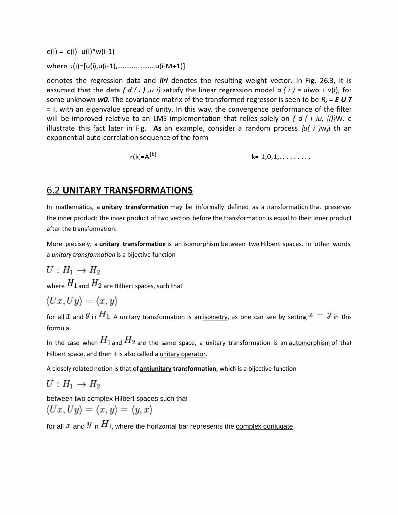
e(i) = d(i)- u(i)*w(i-1)

where u(i)=[u(i),u(i-1),…………………u(i-M+1)]

denotes the regression data and iiri denotes the resulting weight vector. In Fig. 26.3, it is assumed that the data d ( i ) ,u i satisfy the linear regression model d ( i ) = uiwo + v(i), for some unknown w0. The covariance matrix of the transformed regressor is seen to be R, = E U T = I, with an eigenvalue spread of unity. In this way, the convergence performance of the filter will be improved relative to an LMS implementation that relies solely on d ( i )u, (i)W. e illustrate this fact later in Fig. As an example, consider a random process u( i )wi th an exponential auto-correlation sequence of the form r(k)=A|k| k=-1,0,1,. . . . . . . . .

6.2 UNITARY TRANSFORMATIONS

In mathematics, a unitary transformation may be informally defined as a transformation that preserves

the inner product: the inner product of two vectors before the transformation is equal to their inner product

after the transformation.

More precisely, a unitary transformation is an isomorphism between two Hilbert spaces. In other words,

a unitary transformation is a bijective function

where and are Hilbert spaces, such that

for all and in . A unitary transformation is an isometry, as one can see by setting in this

formula.

In the case when and are the same space, a unitary transformation is an automorphism of that

Hilbert space, and then it is also called a unitary operator.

A closely related notion is that of antiunitary transformation, which is a bijective function

between two complex Hilbert spaces such that

for all and in , where the horizontal bar represents the complex conjugate.

Since the statistics of the input data are rarely known in advance, and since the data itself may not even be stationary, the design of a pre-whitening filter l / A ( t) is usually not possible in the manner explained above. Still, there are ways to approximately pre-whiten the data, with varied degrees of success depending on the nature of the data. One such way is to transform the regressors prior to adaptation by some pre-selected unitary transformation, such as the DFT or the DCT, as we now explain.

6.3 DFT LMS Consider the standard LMS implementation

W(i)=w(i-1)+µ*u(i)*[d(i)-u(i)w(i-1)]…………………(1) with regressor ui and associated covariance matrix R = Eu*ui. Let T denote an arbitrary unitary matrix of size M x M , i.e., TT' = T*T = I. For example, T could be chosen in terms of the discrete Fourier transform matrix (DFT), (1/√M )*(e^-j2πmk/M) K,m=0,1,2,………………………………M-1

The appropriate choice of scaling to achieve unitarity is , so that the energy in the

physical domain will be the same as the energy in the Fourier domain, i.e., to satisfy Parseval's

theorem. (Other, non-unitary, scalings, are also commonly used for computational

convenience; e.g., the convolution theorem takes on a slightly simpler form with the scaling

shown in the discrete Fourier transform article.)

6.3 DCT LMS

The DCT can be written as

α(k) * cos(k(2m+1)π/2*M) k,m=0,1,2,……………..M-1

where α(0)=1/√M

and α(k)=√2/M

A discrete cosine transform (DCT) expresses a finite sequence of data points in terms of a sum

of cosine functions oscillating at different frequencies. DCTs are important to numerous

applications in science and engineering, from lossy compression of audio (e.g. MP3)

and images (e.g. JPEG) (where small high-frequency components can be discarded), to spectral

methods for the numerical solution of partial differential equations.[3] The use of cosine rather

than sine functions is critical in these applications: for compression, it turns out that cosine

functions are much more efficient (as described below, fewer functions are needed to

approximate a typical signal), whereas for differential equations the cosines express a particular

choice of boundary conditions.

In particular, a DCT is a Fourier-related transform similar to the discrete Fourier

transform (DFT), but using only real numbers. DCTs are equivalent to DFTs of roughly twice the

length, operating on real data with even symmetry (since the Fourier transform of a real and

even function is real and even), where in some variants the input and/or output data are

shifted by half a sample.

ALGORITHM (DFT domain LMS) 1.The weight vector wo can be approximated iteratively via wi = Fmi, where F is the unitary DFT matrix and W(i) is updated as follows. Define the M x M diagonal matrix. S=diag1,e^-j2π/M,e^-j4π/M,………………………e^-j2π(m-1)/M 2.Then start with Xk(-l) = 6 (a small positive number), 2sr-1 = 0, E-1 = 0, and repeat for i >=0: 3.u(i)=u(i-1)*S + 1/√M u(i)-u(i-M [111…………….1] 4.u(k)=kth entry of u(i) 5.λ(k) = β*λ(i-1) + (1-β) * |u(k)|^2 6. Di = diagλ(i) 7.e(i) = d ( i ) – u(i)*W(i-1) 8.w(i)=w(i-1)+µ*(D^-1)*(e*(i))*u(i) where µ is a positive step-size (usually small) and 0 << p < 1. The computational cost of this algorithm is O(M) operations per iteration.

MATLAB CODE

clc; close all; clear all;

%%%%%%%%%%%%%%%%%%%%%%%%%%%%%%%%%%%%%%%%%%%%%%%%%%%%%%%%%%%% M=3; for k=1:M for m=1:M F(k,m)=(1/sqrt(M))*exp((-2*j*pi*(m-1)*(k-1))/M); end end for m=1:M a(m)=exp((-2*j*pi*(m-1))/M); end %%%%%%%%%%%%%%%%%%%%%%%%%%%%%%%%%%%%%%%%%%%%%%%%%%%%%%%% %signal generation yslide=zeros(1,3); mu=0.2; n=200; u=randn(1,n); h=[0.26 0.93 0.26] for i=1:n yslide(2:3)=yslide(1:2); yslide(1)=u(i); d(i)=yslide*h'; end %%%%%%%%%%%%%%%%%%%%%%%%%%%%%%%%%%%%%%%%%%% xslide=zeros(1,3); S=diag(a); lamda=0.01*ones(1,M); wbar=zeros(M,1); ubar=zeros(1,M); beta=0.8; ubar=zeros(1,3); for i=1:n p=xslide; xslide(2:3)=xslide(1:2); xslide(1)=u(i); % ubar=xslide*F ubar=ubar*S+(1/sqrt(M))*(xslide(1)-p(3))*ones(1,M); % pause lamda=beta*lamda+(1-beta)*(abs(ubar.^2)); D=diag(lamda); ubar*wbar; e(i)=d(i)-ubar*wbar; wbar=wbar+mu*inv(D)*ubar'*e(i);

sqerror(i)=e(i)^2; end v=F*wbar hold on plot(v) % subplot(1,1,1) plot(d,'r'); title('System output') ; xlabel('Samples') ylabel('True and estimated output') figure %subplot(1,2,1); semilogy((abs(e))) ; title('Error curve') ; xlabel('Samples') ylabel('Error value') figure %subplot(1,2,2); plot(h, 'k+') hold on axis([0 6 0.05 0.35])

OUTPUT:

h = 0.2600 0.9300 0.2600 v = 0.2600 - 0.0000i 0.9300 + 0.0000i 0.2600 - 0.0000i

0 20 40 60 80 100 120 140 160 180 20010

-16

10-14

10-12

10-10

10-8

10-6

10-4

10-2

100

Error curve

Samples

Err

or

valu

e

0 20 40 60 80 100 120 140 160 180 200-2.5

-2

-1.5

-1

-0.5

0

0.5

1

1.5

2

2.5System output

Samples

Tru

e a

nd e

stim

ate

d o

utp

ut

Algorithm of DCT DOMAIN LMS

The weight vector wo can be approximated iteratively via wi = CT w(i) where C is the unitary DCT matrIx and w(i) is updated as follows. Define the M x M diagonal matrix: S = diag(2cos (kπ/M), k = (0 , 1 , . . . . . . . . . . . . , M - 1) Then start with λk(-1) = € (a small positive number), w(-1) = 0, u(-1) = 0, and repeat for i >= 0: 1.a(k) = (u[i]-u[i-1])*cos (k*π/2M) k = (0 , 1 , . . . . . . . . . . . . , M - 1) 2.b(k) =(-1)^k * [u(i-M)-u(i-M-1] *cos(k*π/2M) 3.Ω(k) =[a(k)-b(k)]*α(k) 4.U(i)=u(i-1)*S – u(i-2) + [Ω(0) Ω(1) Ω(2). . . . . . . . . . . . . Ω(M-1)] 5.Ui(k) =kth entry of u(i) 6.λ k ( i ) =βλ k(i-1) + (1-β)* |u (k)|^2 7.Di =diag(λk(i)) 8.e ( i ) =d(i)-u(i)*w(i-1) 9.w(i)=w(i-1)+ µ* D^(-1)* u(i)**e(i) where µ is a positive step-size (usually small) and 0 << β < 1. The computational cost of this algorithm is O ( M ) operations per iteration. Figure compares the performance of three LMS implementations for a first-order auto-regressive process u(i) with a in chosen as 0.8. The filter order is set to M = 8 and the ensemble average learning curves are generated by averaging over 300 experiments. The step-size is set to 0.01 and the noise variance at -40 dB. It is seen from the figure that DCT-LMS and DFTLMS exhibit faster convergence.

clc clear all close all M=3; for k=1:M s(k)=2*cos(k*3.14/M); r(k)=cos(k*3.14/(2*M)); end s n=200; a=randn(1,n); u=zeros(1,3); h=[0.1 0.2 0.3]; for i=1:n u(2:3)=u(1:2); u(1)=a(i); d(i)=u*h'; end e=diag(s); e xslide=zeros(1,3); ubar=zeros(1,M); wbar=zeros(M,1); beta=0.4 lamda=0.01*ones(1,M); mu=0.4; for i=1:n for k=1:M p=xslide; xslide(2:3)=xslide(1:2); xslide(1)=a(i); v(k)=(xslide(k)-p(k))*cos(r(k)); b(k)=((-1)^k)*(xslide(1)-p(3))*cos(r(k)); c(k)=((2/M)^0.5)*(v(k)-b(k)); ubar=ubar*e-ubar+c(k); lamda=beta*lamda+(1-beta)*(abs(ubar.^2)); D=diag(lamda); f(i)=d(i)-ubar*wbar; wbar=wbar+mu*inv(D)*ubar'*f(i); sqerror(i)=f(i)^2; end end wbar D

hold on plot(d) plot(c,'r'); title('System output') ; xlabel('Samples') ylabel('True and estimated output') figure semilogy((abs(sqerror(i)))) ; title('Error curve') ; xlabel('Samples') ylabel('Error value') figure plot(h, 'k+') hold on %axis([0 6 0.05 0.35]) for j=1:1000 x=randn(1000,1); u=.05; %input('Enter the value of mu:\n'); wopt=[4;5;6]; w=[0;0;0]; l=length(x); A=zeros(3,1); for i=1:l A(2:3)= A(1:2); A(1)=x(i); d(i)=wopt'*A+rand(1); y(i)=w'*A; e(j,i)=d(i)-y(i); w=w+u*e(j,i)*A; end end MSE1=sum(e.^2); semilogy((abs(MSE1)),'--r') ; %%plot(MSE1,'-b'); hold on; semilogy((abs(e)),'-g') ; %hold on leg=legend('LMS','DCTLMS');

OUTPUT:

CONCLUSION: From the given simulations it can be found that DCT LMS converges faster than the normal LMS algorithm.

0 100 200 300 400 500 600 700 800 900 100010

-35

10-30

10-25

10-20

10-15

10-10

10-5

100

105

Samples

Err

or

valu

e

LMS

DCTLMS

CHAPTER 7

IMPLEMENTATION OF FREQUENCY DOMAIN SYSTEM IDENTIFICATION IN JAMMING

FREQUENCY DOMAIN NLMS ALGORITHM FOR ENHANCED JAM RESISTANT GPS RECEIVER

An optimal beamformer attempts to increase SNR at the array output by adapting its pattern to minimize some cost function.This is to say that, the cost function is inversely associated with the quality of the signal.[1] Therefore by minimizing the cost function we can maximize signal at the array output. The primary optimal beamforming technique discussed in this paper will be MMSE, LMS, Frequency Domain LMS for GPS multipath reduction. In case of a GPS satellite, the DOA of the desired signal is mathematically known because the position of a satellite in an orbit is fixed at a particular time instant. So in some particular adaptive antenna algorithm the DOA of the desired signal is directly given as input.

ADAPTIVE ARRAY PROCESSOR

e(t) = u(t) − whx(t)

e(t)2 = (u(t) − whx(t))2

E[e2(t)] = E[u2(t)] – 2whz+ whRw

Where

z = E[x(t)u∗(t)] is cross correlation between the reference signal and the array signal vector x(t)

R = e[x(t)xH(t)] is the correlation matrix of the array output signal

E[.] is the ensemble mean,

The need for an adaptive beamforming algorithm solution is obvious, once we put a GPS

receiver in a jamming environment is seldom constant in either terms of time or space, so the

MMSE technique is not desirable to solve the normal equation directly. Since the DOA of the

GPS signal & interferer signal both are time variable, the solution for weight vector must be

updated.[12] Furthermore, since the data required estimating the optimal solution is noisy, it is

desirable to use an update equation, which uses previous solutions for the weight vector to

smooth the estimate of the optimal response, reducing the effect of interference.

MODIFIED LMS ALGORITHM USED

The step size parameter μ governs the stability, convergence time and fluctuations of LMS adaptation process. One effective approach to overcome this dependence is to normalize the update step size with an estimate of the input signal variance σ^2u(t). Hence the weight update formula modified as w(t + 1 )= w(t) +( μ/N*(σ^2))*x(t)*e∗(t) where N is the tap length of the spatial filter . This modification leads to the asymptotic performance of the number of taps N. hence convergence is strongly dependent on number of taps N. For large number of taps results is poorer i.e., poorer convergence rate. The use

of active tap algorithm consistently improves the convergence rate of NLMS algorithm.

In frequency domain the above equation reduces to W(k + 1 )= W(k) + μ*X(k)e∗(k)/N N----Number of taps

SIMULATIONS AND RESULTS

POLAR PLOT OF FDNLMS BEAM PATTERN FOR ARRAY ANTENNA

0.2

0.4

0.6

0.8

1

30

210

60

240

90

270

120

300

150

330

180 0

System output

Samples

Tru

e a

nd e

stim

ate

d o

utp

ut

0 20 40 60 80 100 120 140 160 180 2000

0.1

0.2

0.3

0.4

0.5

0.6

0.7System output

Samples

Tru

e a

nd e

stim

ate

d o

utp

ut

CONCLUSION:

System identification can be implemented using various algorithms like LMS,NLMS,SLMS(in time domain)and DFT LMS,DCT LMS(in frequency domain).All these algorithms were simulated in MATLAB and results of their convergence behavior was studied briefly. It was found that NLMS showed the fastest convergence behavior followed by LMS and then by SLMS. The error performance for a one step predictor was calculated both mathematically and also simulated in MATLAB. It was found that results from both of the methods were same and the error performance surface was then implemented in MATLAB. Implementing a jam resistant GPS receiver using FDNLMS was also done and simulation results showed that the proposed method is a viable solution to increase the SNR in the presence of a short delay multipath environment. The combined characteristic of this study prevails over those of other techniques available presently. In addition, the prerequisite of short delay multipath causes the influences of hardware complexity in the FDNLMS adaptive filter to be insignificant. Therefore, the proposed method is a well-suited and well-balanced application in multipath mitigation. This method of enhancing signals using JAM resistant GPS receiver is being widely used nowadays in various defence applications by many developing countries of the world.

REFERENCES AND BIBILIOGRAPHY

[1]A. Kundu and A. Chakrabarty , “FREQUENCY DOMAIN NLMS ALGORITHM FOR ENHANCED

JAM RESISTANT GPS RECEIVER”, Progress In Electromagnetics Research Letters, Vol. 3, 69–78,

2008.

[2].Gu, Y.-J., Z.-G. Shi, K. S. Chen, and Y. Li, “Robust adaptive beamforming for steering vector

uncertainties based on equivalent DOAs method,” Progress In Electromagnetics Research, Vol.

79,2010

[3]Priyanka Yadav and Prof. Smita Patil ,”A COMPARATIVE BEAMFORMING ANALYSIS OF LMS &

NLMS ALGORITHMS FOR SMART ANTENNA “,International Journal of Advanced Research in

Computer Engineering & Technology (IJARCET) Volume 2 Issue 8, August 2013.

[4] G.C. Goodwin and M. Salgado. Frequency domain sensitivity functions for continuous time systems under sampled data control. Automatica, Vol. 30,100-110,August 1994. [5]M.Grattan-Guinness. Convolutions in French mathematics, 1800-1840, Vol. 2. Birkh¨auser Verlag,120-124,1990. [6] W.M. Haddad, H.H. Huang, and D.S. Berstein. Sampled-data observers with generalized holds for unstable plants. IEEE Trans. on Automatic Control, Vol. 39(1): 229–234, January 2000. [7] S. Lee and Y. Lee, “Adaptive frequency hopping for bluetooth robust to WLAN interference,” IEEE Communications Letters, vol. 13, pp. 628–630, September 2009 [8] A. Shokrollahi, “Raptor codes,” IEEE Transactions on Information Theory,Vol. 52, pp. 2551–2567, June 2006.100 [9] B. Peeters and G. De Roeck. Reference-based stochastic subspace identification for output only modal analysis. Mechanical Systems and Signal Processing, Vol. 13(6),pp. 855–878, 1999. [10] R. Pintelon, P. Guillaume, G. Vandersteen, and Y. Rolain. Analysis, development and applications of tls algorithms in frequency domain system identification. Proceedings of the Second International Workshop on Total Least Squares and Errors-in-Variables Modeling,Vol 12 pages 341–358, 1996. [11] Jr. S. Lawrence Marple. Digital Spectral Analysis. Prentice-Hall,Vol.34,1987. [12] B. Peeters and G. De Roeck. Stochastic system identification for operational modal analysis: A review. Journal of Dynamic Systems, Measurements, and Control, 2002.

[13] R. Pintelon. Frequency-domain subspace system identification using non-parametric noise models. Automatica, Vol 38,pp 295–311, 2002. [14] R. Starc and J. Schoukens. Identification of continuous-time systems using arbitrary signals. Automatical,Vol 33(5):pp 91–94, 1997. [15] R. Pintelon and K. Smith Time series analysis in the frequency domain. IEEE Transactions on Signal Processing,Vol 47, No. 1, 1999. [16]R. Ruotolo. A multiple-input multiple-output smoothing technique: Theory and application to aircraft data. Journal of Sound and Vibration, Vol 247(3):453–469, 2001. [17]J. Schoukens, Y. Rolain, J. Swevers, and J. De Cuyper. Simple methods and insight to deal with nonlinear distortions in frf measurements. Radar Systems and Signal Processing,Vol 14(4):657–666, 2000. [18] P. Van Overschee and B. De Moor. Subspace algorithms for the stochastic identification problem. Automatica, 29(3):649–660, 1993 [19]P. Van Overschee and B. De Moor. Subspace Identification for Linear Systems: Theory Implemantation-Applications. Kluwer Academic Publishers,Vol. 67,pp 67-69,1996.. [20] P. Verboven, E. Parloo, P. Guillaume, and M. Van Overmeire. Autonomous structural health monitoring - part i: Modal parameter estimation and tracking. Electrical Systems and Signal Processing, Vol 56,pp 67-69, 2003.