Journal of Environmental Protection, 2014, 5, 845-861 Published Online July 2014 in SciRes. http://www.scirp.org/journal/jep http://dx.doi.org/10.4236/jep.2014.510087

How to cite this paper: Hamdy, D., Moustafa, M.A.E. and Elbakri, W. (2014) Free Residual Chlorine Calibration by Water-CAD at El-Nozha Water Network in Alexandria Governorate, Egypt. Journal of Environmental Protection, 5, 845-861. http://dx.doi.org/10.4236/jep.2014.510087

Free Residual Chlorine Calibration by WaterCAD at El-Nozha Water Network in Alexandria Governorate, Egypt Diaa Hamdy, Medhat A. E. Moustafa, Walid Elbakri Sanitary Engineering Department, Faculty of Engineering, University of Alexandria, Alexandria, Egypt Email: diaahamdy55@gmail.com, medhat002000@yahoo.com, welbarki76@gmail.com Received 24 April 2014; revised 21 May 2014; accepted 13 June 2014

Copyright © 2014 by authors and Scientific Research Publishing Inc. This work is licensed under the Creative Commons Attribution International License (CC BY). http://creativecommons.org/licenses/by/4.0/

Abstract Most of developing countries suffer from decreasing and poor quality of drinking water which led to emergence of many dangerous diseases. In addition, there isn’t any methodology followed to predict and disinfect drinking water by using advanced software program. Maintaining water quality in the water distribution system has become a prominent issue in the study of the water network. Residual chlorine concentration is the indicator to ensure the quality of water in the wa-ter network because it eliminates contaminants in the distribution network beginning of the treat- ment plant down to the consumer. In collaboration with Alexandria (Egypt) Water Company, sam-ples were taken from El-NOZHA water plant station and El-HADARA water distribution network to know the free residual chlorine. In this paper, WaterCAD software has been used to make hydrau-lic analysis and calibration of residual chlorine in water distribution network to know the ideal chlorine dose that should be added at the water treatment plant and to know the areas of strength and weakness in the concentration of free residual chlorine in the water distribution network. In addition different scenarios have been found to know the free residual chlorine at the weakness areas after injecting chlorine in some junctions and the impact of a fire case or breaking in the water pipe distribution network on the residual chlorine. Results showed ensuring in the water quality in the distribution network by adding chlorine dose in water less than the existing dose which has been added in the El-NOZHA water treatment plant. It is possible to maintain the per-centage of free residual chlorine concentration at different locations without relying on adding chlorine only in water treatment plant by injecting low percentage of chlorine dose in the junc-tions.

Keywords Water Distribution System, Residual Chlorine Concentration (RCC), WaterCAD, Supervisory

D. Hamdy et al.

846

Control and Data Acquisition (SCADA), Geographic Information System (GIS), Water Treatment Plant (WTP)

1. Introduction Water is essential for all forms of life on the earth. A human can survive for weeks without food but only a few days without water. The water is essential for growth and preserves our bodies. The treated water which does not contain any contaminates revives and heals our body from many diseases. On the contrary if the water is polluted that’s a case setback in human health and cause many diseases that are known today [1]. Disinfection is an important step in ensuring that water is safe to drink. Water treatment plants add disinfectants to destroy mi-croorganisms that can cause disease in humans. There are several methods of disinfection\n such as chlorination, chloramines, ozone, and ultraviolet light. Other disinfection methods include chlorine dioxide, potassium per-manganate, and nanofiltration [2]. The most important methods of disinfection are chlorine dioxide (the most common disinfection method). The chlorine was discovered in 1774 by Carl Wilhelm Scheele [3]. The first use was as a weapon against humans in World War I by Germany. After that, scientists knew its advantages and its effectiveness in water disinfection [4]. Water quality management has become very important, especially with the spread of diseases transmitted by water. Computer software lets sanitary engineering make more controls at water disinfection and ensure water quality for the customer. The Alexandria Water Company setup plans to develop control methods at water quality management which includes: Application of computer software to develop the water plant station control. Using GIS and SKADA system to know strengths and weaknesses at distribution system. Encouragement scientific research and analysis of the results by using advanced software. Obtaining international certification at water quality control.

This research focuses on the water quality control by measuring the residual chlorine concentration in water distribution system and calibrates the doses system to reach the optimal chlorine dose.

2. Materials and Methods 2.1. Study Area Alexandria city consists of six districts (Table 1) in addition to Burj Al Arab city. These districts are divided in-to sixteen administrative sections. The Alexandria total area is 723,271 acres of which 73,392 acres is a con-struction area and represents 10.15% from the total area of the province. The other areas are deserts lands, agri-cultural land and surface water (Lake Mareotis) [5].

In 2007 the total population was 194.206 which represent about 32.3% of the total population of the middle district. The section consists of six subsections; it’s called Sheyakha. The total population for each subsection is shown in (Table 2) [6].

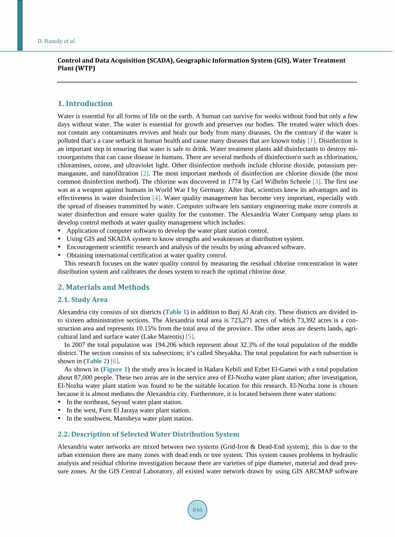
As shown in (Figure 1) the study area is located in Hadara Kebili and Ezbet El-Gamei with a total population about 87,000 people. These two areas are in the service area of El-Nozha water plant station; after investigation, El-Nozha water plant station was found to be the suitable location for this research. El-Nozha zone is chosen because it is almost mediates the Alexandria city. Furthermore, it is located between three water stations: In the northeast, Seyouf water plant station. In the west, Furn El Jaraya water plant station. In the southwest, Mansheya water plant station.

2.2. Description of Selected Water Distribution System Alexandria water networks are mixed between two systems (Grid-Iron & Dead-End system); this is due to the urban extension there are many zones with dead ends or tree system. This system causes problems in hydraulic analysis and residual chlorine investigation because there are varieties of pipe diameter, material and dead pres-sure zones. At the GIS Central Laboratory, all existed water network drawn by using GIS ARCMAP software

D. Hamdy et al.

847

Table 1. Alexandria districts.

District Area (acre) Urban construction space (acre)

Percentage from the total area

Montaza 25,530 8697 43.1%

East 13,685 1697 12.4%

Middle 9640 1711 17.75%

West 7627 1849 24.1%

El Gomrok 1102 642 58.3%

Amriya 581,000 56,558 9.7%

Burj Al-Arab 84,642 2238 2.6%

Table 2. Sheyakhat population at eastern section.

Sheyakha Population

Ibrahimiya Bahary 28,122

Ibrahimiya Kebili and Hadara Bahary 53,894

Azarita and Shatby 16,134

Hadara Kebili (study area) 56,631

Bab Sharky & Wabour El Maya 9083

Ezbet El-Gamei (study area) 30,342

Figure 1. Map showing the location of the study area.

D. Hamdy et al.

848

version 10. This facility provides the engineers and the technicians to do surveys for the water network to know detailed information about network type, diameter, length and age. Also, they can record any pipe replacement and renewal, to enable them to develop future plan, and identify the strength and weakness parts in Alexandria water company (AWCO) service area [5] [7].

2.3. Locations & Dates of Sampling Points This section covers the selection criteria of sampling points, which called lab samples in this search. The con-sideration about sampling is detailed in these following lines: The lab samples should be from multiple areas (near, centre & far) from the water plant station. The lab samples are from closed zone areas to avoid the effect of residual chlorine dose in water network

from another water station. Selected areas should have varieties of pipe material, to know the effective of the each pipe martial (wall

reaction) on the residual chlorine. Samples also should be from the dead end of pipe to ensure the residual chlorine percentage. Samples also should be taken from the water treatment plant to know the residual chlorine dose before its in-

teraction in the water distribution network. In order to maintain the above criteria, thirty three locations were selected from various parts of the studied area.

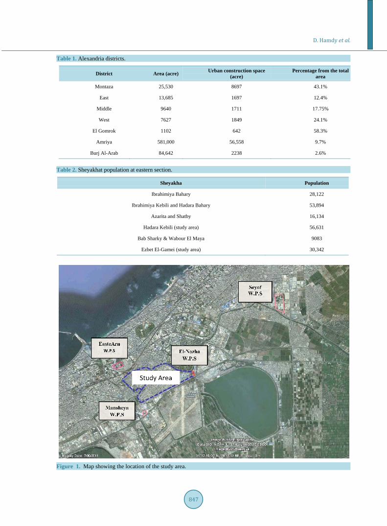
Samples were collected from the actual water consumption tap that may be at restaurant, shops or other activity place, in addition other locations were selected in a specific area which is nearly from El-Nozha water plant station as shown in (Figure 2).

Four months throughout the year were chosen (December, January, April & July), and samples were taken along the month to know the actual residual chlorine concentration in water network. These months were chosen to cover all probable seasonal variations. Total numbers of the samples were about two hundred and sixty sam-ples per month. Samples were collected two times daily; the first time at eleven o’clock a.m. and the second time at four o’clock p.m. These two times were chosen to know the chlorine concentration at two different times during the day. Samples were also taken from the water plant, which is the main source of chlorine.

2.4. Analysis Tool The WaterCAD versions started from (V4) to latest version (V8i). Each version has new options and more pos-sibilities to be useful to any sanitary engineer to do complex hydraulic analysis and ensure water quality in any

Figure 2. Lab samples locations and service area.

D. Hamdy et al.

849

distribution system. In this work Bentely WaterCAD (V8i) has been used. This software is used to perform steady-state and extended hydraulic analysis of water distribution network.

The steady state analysis determines the operating behavior of the system at a specific point in time or under steady-state conditions (flow rates and hydraulic grades remain constant over time). This type of analysis is useful for determining pressures and flow rates under minimum, average, peak, or short term effects on the system due to fire flows. For this type of analysis, the network equations are determined and solved with tanks being treated as fixed grade boundaries. The results that are obtained from this type of analysis are instantaneous values and may or may not be representative of the values of the system a few hours, or even few minute.

The extended state type of analysis allows engineer to model tanks filling and draining, regulating valves opening and closing, and pressures and flow rates changing throughout the system in response to varying demand conditions and automatic control.

WaterCAD also perform water quality simulations to determine the water source and age, or track the growth or decay of a chemical constituent throughout the network, perform fire flow analysis on the system to determine how it will behave under extreme conditions.

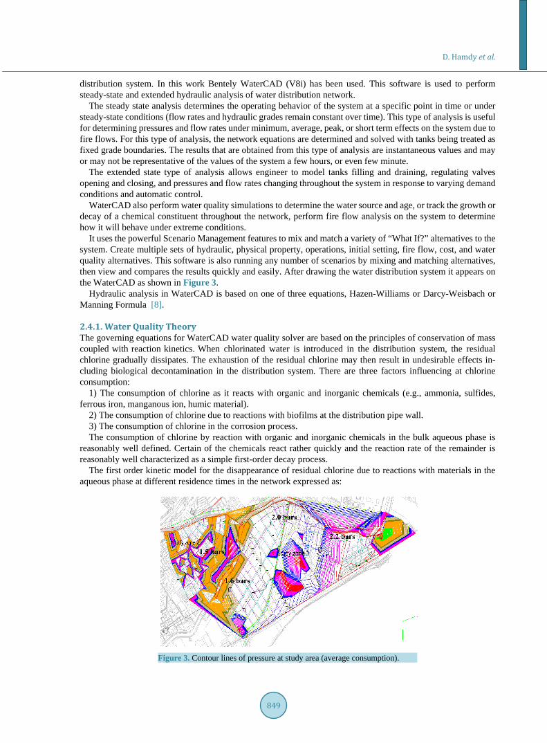
It uses the powerful Scenario Management features to mix and match a variety of “What If?” alternatives to the system. Create multiple sets of hydraulic, physical property, operations, initial setting, fire flow, cost, and water quality alternatives. This software is also running any number of scenarios by mixing and matching alternatives, then view and compares the results quickly and easily. After drawing the water distribution system it appears on the WaterCAD as shown in Figure 3.

Hydraulic analysis in WaterCAD is based on one of three equations, Hazen-Williams or Darcy-Weisbach or Manning Formula [8].

2.4.1. Water Quality Theory The governing equations for WaterCAD water quality solver are based on the principles of conservation of mass coupled with reaction kinetics. When chlorinated water is introduced in the distribution system, the residual chlorine gradually dissipates. The exhaustion of the residual chlorine may then result in undesirable effects in-cluding biological decontamination in the distribution system. There are three factors influencing at chlorine consumption:

1) The consumption of chlorine as it reacts with organic and inorganic chemicals (e.g., ammonia, sulfides, ferrous iron, manganous ion, humic material).

2) The consumption of chlorine due to reactions with biofilms at the distribution pipe wall. 3) The consumption of chlorine in the corrosion process. The consumption of chlorine by reaction with organic and inorganic chemicals in the bulk aqueous phase is

reasonably well defined. Certain of the chemicals react rather quickly and the reaction rate of the remainder is reasonably well characterized as a simple first-order decay process.

The first order kinetic model for the disappearance of residual chlorine due to reactions with materials in the aqueous phase at different residence times in the network expressed as:

Figure 3. Contour lines of pressure at study area (average consumption).

D. Hamdy et al.

850

ddc KCt= −

where c is the chlorine concentration (mg/L) and k is the first-order decay constant (min−1). The residence time is defined as the pipe length divided by the mean flow velocity in the pipe. Integrating equation gives:

( ) 0e ktC t c −=

where C(t) is the chlorine concentration (mg/L) at time t, c0 is the initial chlorine concentration (mg/L), and it is the residence time in the pipe (min). The chlorine decay constant k is site specific and must be verified by field measurements. The k values vary with: The water quality. The water temperature. The flow velocity. The pipe material. The area of contact with the pipe. The second-order rate process expressed as:

( ) ( )2 0

0

dd 1

or Ccc KC

t c tt

K=

+=−

′

where K' is a second-order rate constant. The use of this model was illustrated by Murphy (1985) [9].

2.4.2. Calibration Methodology To ensure a good investment return and correct use of the models, the model should be capable of correctly si-mulating flow conditions encountered at the site. This is achieved by calibrating the models. A calibration in-volves the process of adjusting model characteristics and parameters so that the model’s predicted flows and pressures match actual observed field data.

Calibration of a water distribution model is a complicated task. There are many uncertain parameters that need to be adjusted to reduce the discrepancy between the model predictions and field observations of junction HGL and pipe discharges. Pipe roughness coefficients are often considered for calibration. However, there are many other parameters that are uncertain and affect junction HGL and pipe flow rate such as junction demand, operation status of pipes and valves.

Calibrating water distribution network models relies upon field measurement data, such as junction pressures, pipe flows, and water levels in storage facilities, valve settings, pump operating status (on/off), and pump speeds. Among all the possible field observation data, junction HGL and pipe flows are most often used to evaluate the goodness-of-fit of the model calibration. Other parameters, such as tank levels, valve settings, and pump operating status/speed are used as boundary conditions that are recorded when collecting a set of calibration observations of junction pressures and pipe flow rates.

Traditional calibration of a water distribution model is based on a trial-and-error procedure by which an engi-neer or modeller first estimates the values of model parameters, run the model to obtain a predicted pressure and flow, and finally compares the simulated values to the observed data. If the predicted data does not compare closely with the observed data, the engineer returns to the model, makes some adjustments to the model para-meters, and calculates it again to produce a new set of simulation results. This may have to be repeated many times to make sure that the model produces a calibrated prediction of the water distribution network in the real world [10].

2.4.3. Scenario Management Scenario management feature can dramatically increase the productivity in the “What If?” areas of modelling, including calibration, operations analysis, and planning. The main advantages of scenario management are: A single project file makes it possible to generate an unlimited number of “What If?” conditions without be-

coming overwhelmed with numerous modelling files and separate results. The software maintains the data for all the scenarios in a single project, it can provide with powerful auto-

mated tools for directly comparing scenario results. Any set of results is immediately available at any time. The scenario/alternative relationship empowers to mix and match groups of data from existing scenarios

D. Hamdy et al.

851

without having to re-declare any data. The designer doesn’t have to re-enter data if it remains unchanged in a new alternative or scenario, avoiding

redundant copies of the same data. Inheritance also enables to correct a data input error in a parent scenario and automatically update the corrected attribute in all child scenarios [10].

2.4.4. Contour Map Manager The Contour Map Manager contains the information required to generate contours for a calculated network, or-ganized as follows [11]: Minimum: lowest value to be included in the contour map. Maximum: highest value for which contours will be generated. Increment: step by which the contours increase.

The created contours will be evenly divisible by the increment, and are not directly related to the minimum and maximum values. For example, a contour set with 10 minimum, 20 maximum, and an increment of 3 would result in the following set: [12, 15, 18] not [10, 13, 16, 19].

3. Results and Discussion 3.1. Hydraulic Analysis at Steady State Case The study area is divided in two zones, zone one is located nearly from the NOZHA WTP, so it’s in the circle of influence. Zone two is located nearly the EASTERN WTP. At average consumption rate = 3.04 m3/hr, hydraulic grade & pressure have been calculated. Figure 3 shows the pressures at the two zones by contour lines.

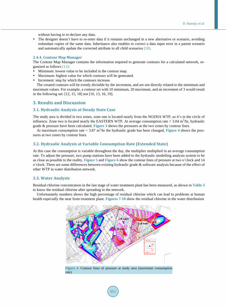
At maximum consumption rate = 3.87 m3/hr the hydraulic grade has been changed, Figure 4 shows the pres-sures at two zones by contour lines.

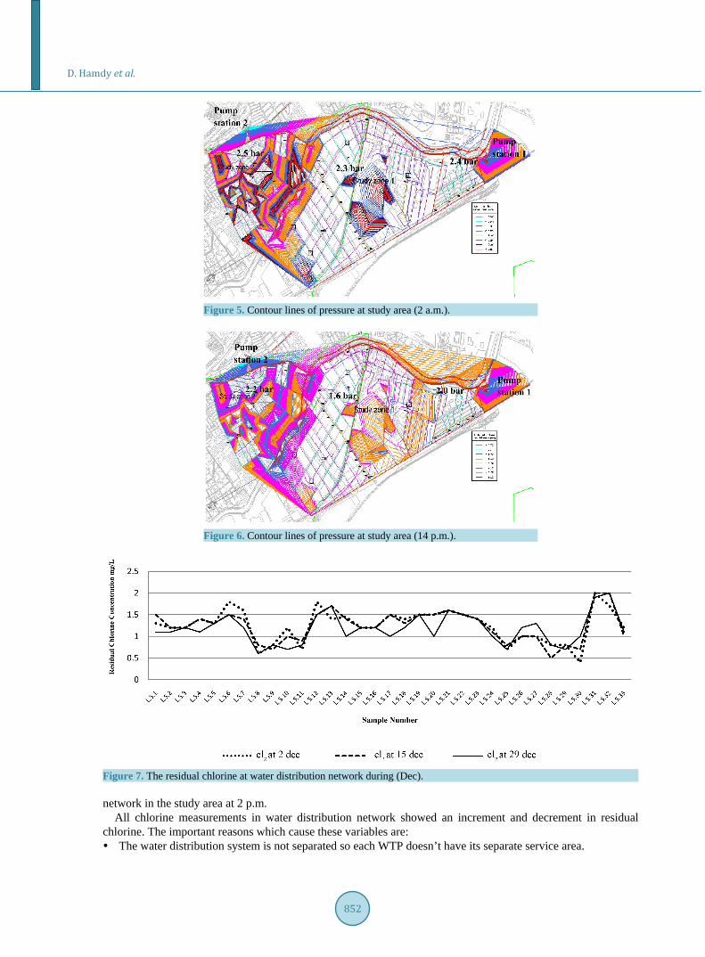
3.2. Hydraulic Analysis at Variable Consumption Rate (Extended State) At this case the consumption is variable throughout the day, the multiplier multiplied in an average consumption rate. To adjust the pressure, two pump stations have been added to the hydraulic modelling analysis system to be as close as possible to the reality. Figure 5 and Figure 6 show the contour lines of pressure at two o’clock and 14 o’clock. There are some differences between existing hydraulic grade & software analysis because of the effect of other WTP in water distribution network.

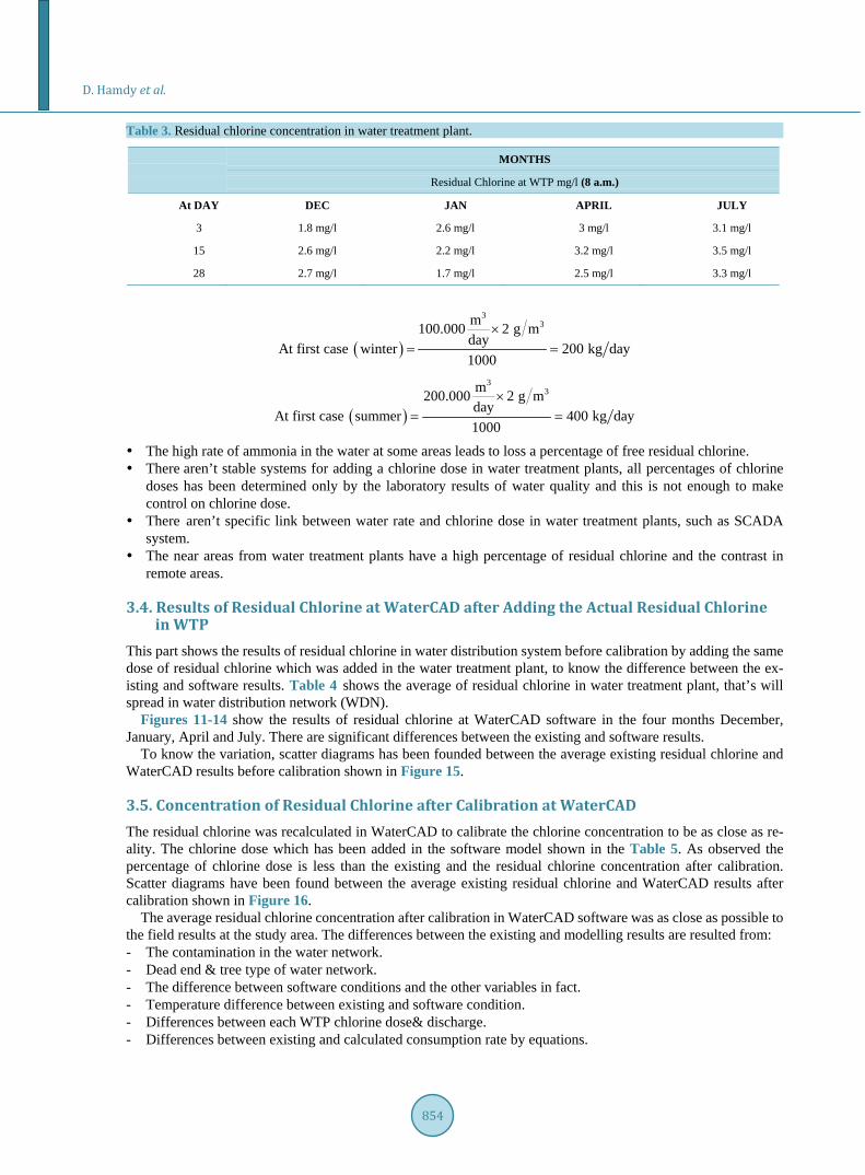
3.3. Water Analysis Residual chlorine concentration in the last stage of water treatment plant has been measured, as shown in Table 3 to know the residual chlorine after spreading in the network.

Unfortunately numbers shows the high percentage of residual chlorine which can lead to problems at human health especially the near from treatment plant. Figures 7-10 show the residual chlorine in the water distribution

Figure 4. Contour lines of pressure at study area (maximum consumption rate).

D. Hamdy et al.

852

Figure 5. Contour lines of pressure at study area (2 a.m.).

Figure 6. Contour lines of pressure at study area (14 p.m.).

Figure 7. The residual chlorine at water distribution network during (Dec). network in the study area at 2 p.m.

All chlorine measurements in water distribution network showed an increment and decrement in residual chlorine. The important reasons which cause these variables are: The water distribution system is not separated so each WTP doesn’t have its separate service area.

D. Hamdy et al.

853

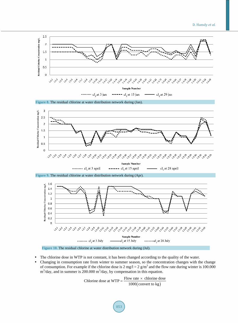
Figure 8. The residual chlorine at water distribution network during (Jan).

Figure 9. The residual chlorine at water distribution network during (Apr).

Figure 10. The residual chlorine at water distribution network during (Jul). The chlorine dose in WTP is not constant, it has been changed according to the quality of the water. Changing in consumption rate from winter to summer season, so the concentration changes with the change

of consumption. For example if the chlorine dose is 2 mg/l = 2 g/m3 and the flow rate during winter is 100.000 m3/day, and in summer is 200.000 m3/day, by compensation in this equation.

( )Flow rate chlorine doseChlorine dose at WTP

1000 convert to kg×

=

D. Hamdy et al.

854

Table 3. Residual chlorine concentration in water treatment plant.

MONTHS

Residual Chlorine at WTP mg/l (8 a.m.)

At DAY DEC JAN APRIL JULY

3 1.8 mg/l 2.6 mg/l 3 mg/l 3.1 mg/l

15 2.6 mg/l 2.2 mg/l 3.2 mg/l 3.5 mg/l

28 2.7 mg/l 1.7 mg/l 2.5 mg/l 3.3 mg/l

( )

33m100.000 2 g m

daAt first case y 200 kg day100

winter0

=×

=

( )

33m200.000 2 g m

daAt first case y 400 kg day100

summer0

=×

=

The high rate of ammonia in the water at some areas leads to loss a percentage of free residual chlorine. There aren’t stable systems for adding a chlorine dose in water treatment plants, all percentages of chlorine

doses has been determined only by the laboratory results of water quality and this is not enough to make control on chlorine dose.

There aren’t specific link between water rate and chlorine dose in water treatment plants, such as SCADA system.

The near areas from water treatment plants have a high percentage of residual chlorine and the contrast in remote areas.

3.4. Results of Residual Chlorine at WaterCAD after Adding the Actual Residual Chlorine in WTP

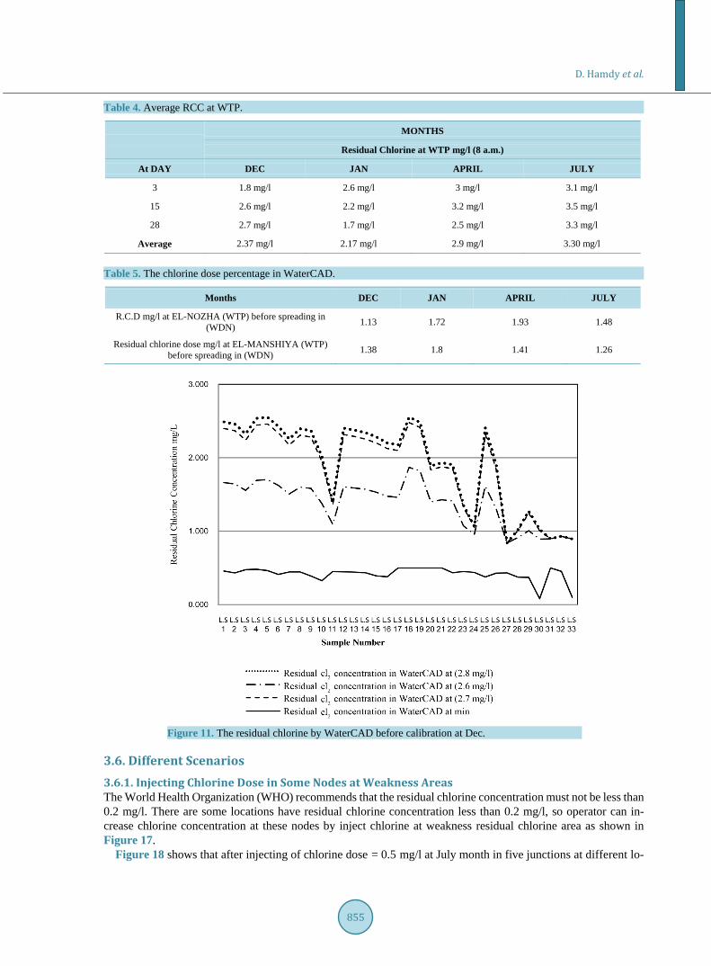
This part shows the results of residual chlorine in water distribution system before calibration by adding the same dose of residual chlorine which was added in the water treatment plant, to know the difference between the ex-isting and software results. Table 4 shows the average of residual chlorine in water treatment plant, that’s will spread in water distribution network (WDN).

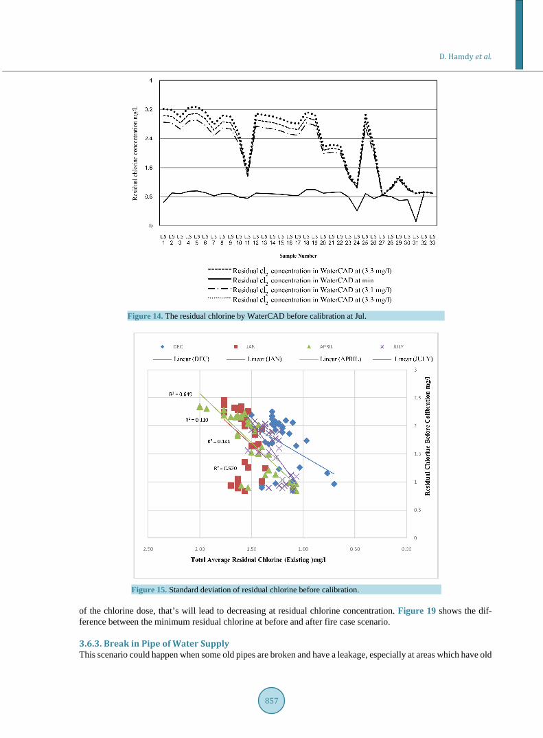
Figures 11-14 show the results of residual chlorine at WaterCAD software in the four months December, January, April and July. There are significant differences between the existing and software results.

To know the variation, scatter diagrams has been founded between the average existing residual chlorine and WaterCAD results before calibration shown in Figure 15.

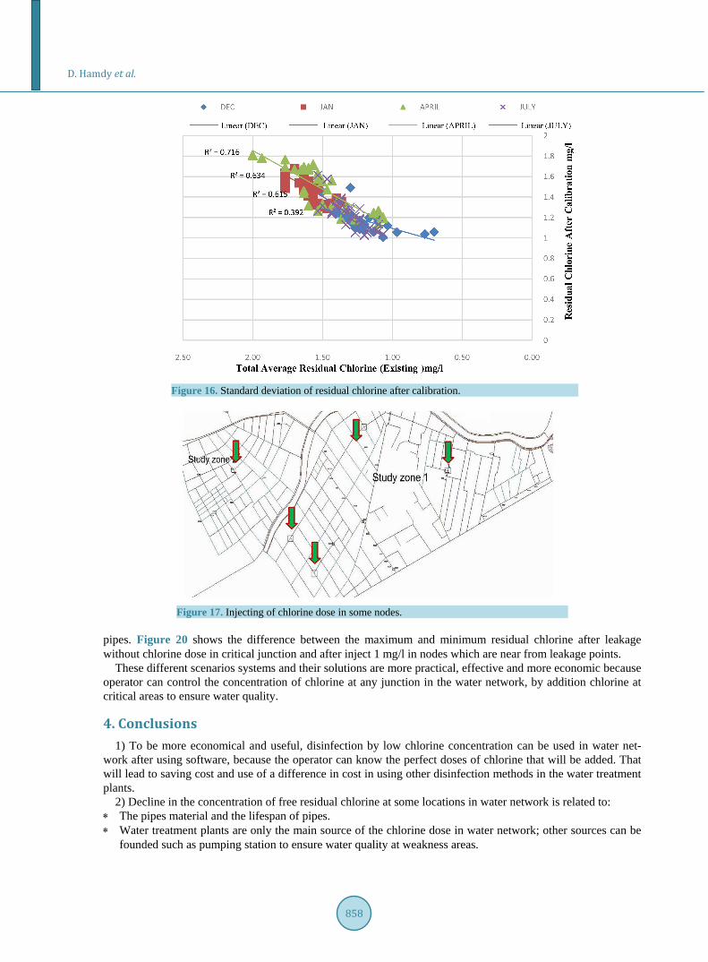
3.5. Concentration of Residual Chlorine after Calibration at WaterCAD The residual chlorine was recalculated in WaterCAD to calibrate the chlorine concentration to be as close as re-ality. The chlorine dose which has been added in the software model shown in the Table 5. As observed the percentage of chlorine dose is less than the existing and the residual chlorine concentration after calibration. Scatter diagrams have been found between the average existing residual chlorine and WaterCAD results after calibration shown in Figure 16.

The average residual chlorine concentration after calibration in WaterCAD software was as close as possible to the field results at the study area. The differences between the existing and modelling results are resulted from: - The contamination in the water network. - Dead end & tree type of water network. - The difference between software conditions and the other variables in fact. - Temperature difference between existing and software condition. - Differences between each WTP chlorine dose& discharge. - Differences between existing and calculated consumption rate by equations.

D. Hamdy et al.

855

Table 4. Average RCC at WTP.

MONTHS

Residual Chlorine at WTP mg/l (8 a.m.)

At DAY DEC JAN APRIL JULY

3 1.8 mg/l 2.6 mg/l 3 mg/l 3.1 mg/l

15 2.6 mg/l 2.2 mg/l 3.2 mg/l 3.5 mg/l

28 2.7 mg/l 1.7 mg/l 2.5 mg/l 3.3 mg/l

Average 2.37 mg/l 2.17 mg/l 2.9 mg/l 3.30 mg/l

Table 5. The chlorine dose percentage in WaterCAD.

Months DEC JAN APRIL JULY

R.C.D mg/l at EL-NOZHA (WTP) before spreading in (WDN) 1.13 1.72 1.93 1.48

Residual chlorine dose mg/l at EL-MANSHIYA (WTP) before spreading in (WDN) 1.38 1.8 1.41 1.26

Figure 11. The residual chlorine by WaterCAD before calibration at Dec.

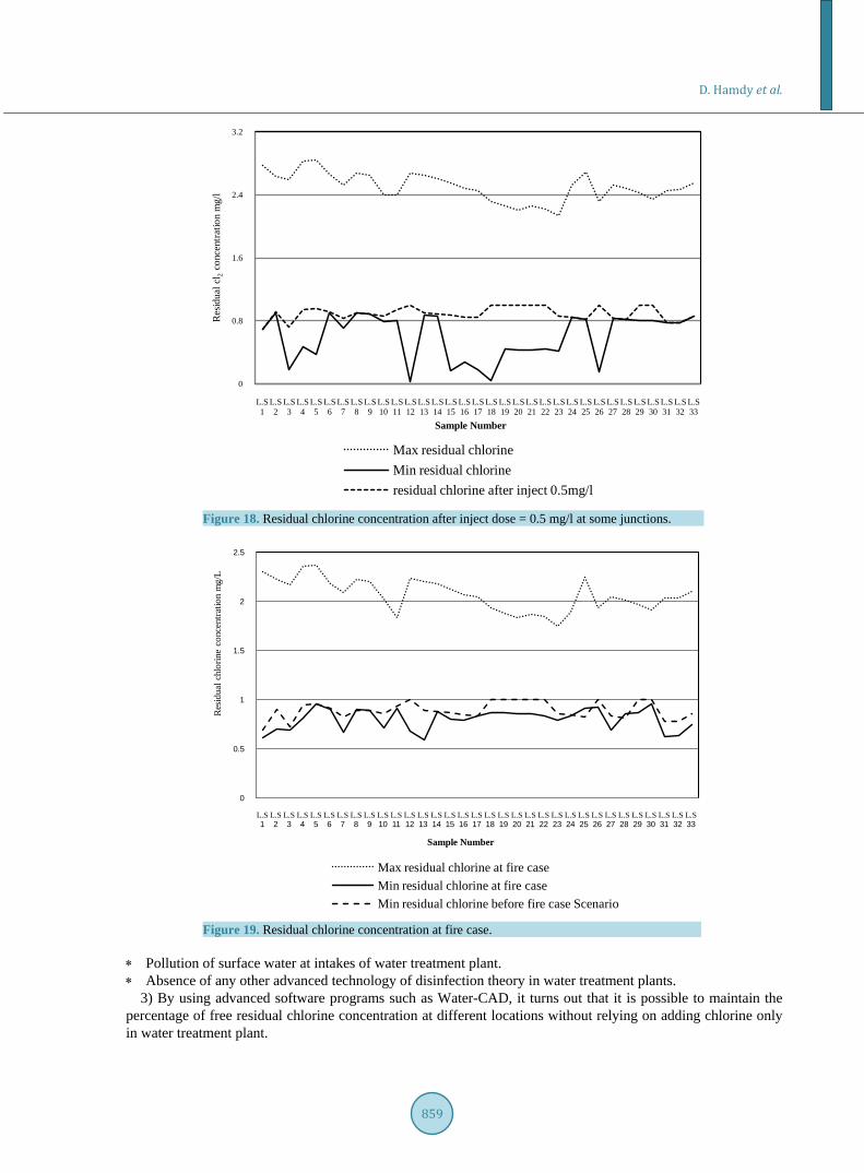
3.6. Different Scenarios 3.6.1. Injecting Chlorine Dose in Some Nodes at Weakness Areas The World Health Organization (WHO) recommends that the residual chlorine concentration must not be less than 0.2 mg/l. There are some locations have residual chlorine concentration less than 0.2 mg/l, so operator can in-crease chlorine concentration at these nodes by inject chlorine at weakness residual chlorine area as shown in Figure 17.

Figure 18 shows that after injecting of chlorine dose = 0.5 mg/l at July month in five junctions at different lo-

D. Hamdy et al.

856

Figure 12. The residual chlorine by WaterCAD before calibration at Jan.

Figure 13. The residual chlorine by WaterCAD before calibration at Apr.

cations, the minimum residual chlorine dose will increase to be at safety level.

3.6.2. Fire Flow Scenario During firefighting time the flow rate in the water network will increase to be about 1189.5 m3/hr. Which will affect on residual chlorine concentration, this case called emergency case. By increasing the rate of water pumping at the treatment plant to avoid the problems of water consumption in water distribution system without increasing

D. Hamdy et al.

857

Figure 14. The residual chlorine by WaterCAD before calibration at Jul.

Figure 15. Standard deviation of residual chlorine before calibration.

of the chlorine dose, that’s will lead to decreasing at residual chlorine concentration. Figure 19 shows the dif-ference between the minimum residual chlorine at before and after fire case scenario.

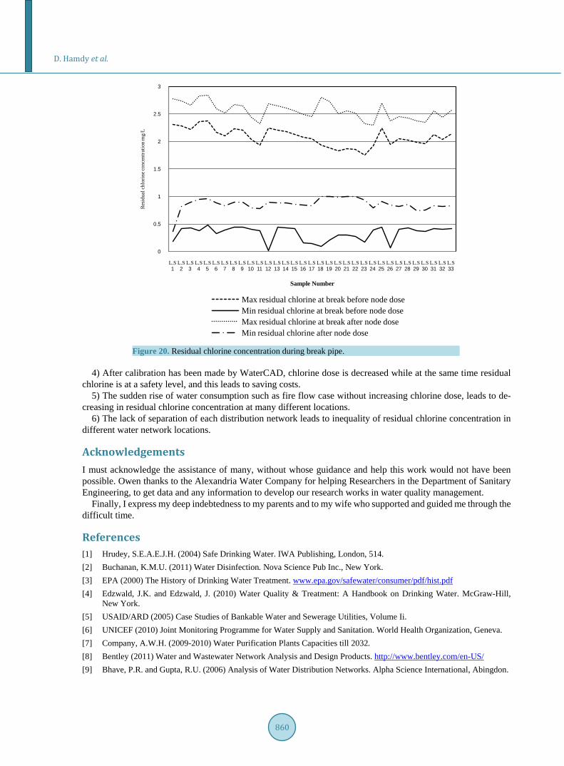
3.6.3. Break in Pipe of Water Supply This scenario could happen when some old pipes are broken and have a leakage, especially at areas which have old

D. Hamdy et al.

858

Figure 16. Standard deviation of residual chlorine after calibration.

Figure 17. Injecting of chlorine dose in some nodes.

pipes. Figure 20 shows the difference between the maximum and minimum residual chlorine after leakage without chlorine dose in critical junction and after inject 1 mg/l in nodes which are near from leakage points.

These different scenarios systems and their solutions are more practical, effective and more economic because operator can control the concentration of chlorine at any junction in the water network, by addition chlorine at critical areas to ensure water quality.

4. Conclusions 1) To be more economical and useful, disinfection by low chlorine concentration can be used in water net-

work after using software, because the operator can know the perfect doses of chlorine that will be added. That will lead to saving cost and use of a difference in cost in using other disinfection methods in the water treatment plants.

2) Decline in the concentration of free residual chlorine at some locations in water network is related to: ∗ The pipes material and the lifespan of pipes. ∗ Water treatment plants are only the main source of the chlorine dose in water network; other sources can be

founded such as pumping station to ensure water quality at weakness areas.

D. Hamdy et al.

859

Figure 18. Residual chlorine concentration after inject dose = 0.5 mg/l at some junctions.

Figure 19. Residual chlorine concentration at fire case.

∗ Pollution of surface water at intakes of water treatment plant. ∗ Absence of any other advanced technology of disinfection theory in water treatment plants.

3) By using advanced software programs such as Water-CAD, it turns out that it is possible to maintain the percentage of free residual chlorine concentration at different locations without relying on adding chlorine only in water treatment plant.

0

0.8

1.6

2.4

3.2

L.S 1

L.S 2

L.S 3

L.S 4

L.S 5

L.S 6

L.S 7

L.S 8

L.S 9

L.S 10

L.S 11

L.S 12

L.S 13

L.S 14

L.S 15

L.S 16

L.S 17

L.S 18

L.S 19

L.S 20

L.S 21

L.S 22

L.S 23

L.S 24

L.S 25

L.S 26

L.S 27

L.S 28

L.S 29

L.S 30

L.S 31

L.S 32

L.S 33

Res

idua

l cl 2

conc

entra

tion

mg/

l

Sample Number

Max residual chlorineMin residual chlorineresidual chlorine after inject 0.5mg/l

0

0.5

1

1.5

2

2.5

L.S 1

L.S 2

L.S 3

L.S 4

L.S 5

L.S 6

L.S 7

L.S 8

L.S 9

L.S 10

L.S 11

L.S 12

L.S 13

L.S 14

L.S 15

L.S 16

L.S 17

L.S 18

L.S 19

L.S 20

L.S 21

L.S 22

L.S 23

L.S 24

L.S 25

L.S 26

L.S 27

L.S 28

L.S 29

L.S 30

L.S 31

L.S 32

L.S 33

Res

idua

l chl

orin

e co

ncen

tratio

n m

g/L

Sample Number

Max residual chlorine at fire caseMin residual chlorine at fire caseMin residual chlorine before fire case Scenario

D. Hamdy et al.

860

Figure 20. Residual chlorine concentration during break pipe.

4) After calibration has been made by WaterCAD, chlorine dose is decreased while at the same time residual

chlorine is at a safety level, and this leads to saving costs. 5) The sudden rise of water consumption such as fire flow case without increasing chlorine dose, leads to de-

creasing in residual chlorine concentration at many different locations. 6) The lack of separation of each distribution network leads to inequality of residual chlorine concentration in

different water network locations.

Acknowledgements I must acknowledge the assistance of many, without whose guidance and help this work would not have been possible. Owen thanks to the Alexandria Water Company for helping Researchers in the Department of Sanitary Engineering, to get data and any information to develop our research works in water quality management.

Finally, I express my deep indebtedness to my parents and to my wife who supported and guided me through the difficult time.

References [1] Hrudey, S.E.A.E.J.H. (2004) Safe Drinking Water. IWA Publishing, London, 514. [2] Buchanan, K.M.U. (2011) Water Disinfection. Nova Science Pub Inc., New York. [3] EPA (2000) The History of Drinking Water Treatment. www.epa.gov/safewater/consumer/pdf/hist.pdf [4] Edzwald, J.K. and Edzwald, J. (2010) Water Quality & Treatment: A Handbook on Drinking Water. McGraw-Hill,

New York. [5] USAID/ARD (2005) Case Studies of Bankable Water and Sewerage Utilities, Volume Ii. [6] UNICEF (2010) Joint Monitoring Programme for Water Supply and Sanitation. World Health Organization, Geneva. [7] Company, A.W.H. (2009-2010) Water Purification Plants Capacities till 2032. [8] Bentley (2011) Water and Wastewater Network Analysis and Design Products. http://www.bentley.com/en-US/ [9] Bhave, P.R. and Gupta, R.U. (2006) Analysis of Water Distribution Networks. Alpha Science International, Abingdon.

0

0.5

1

1.5

2

2.5

3

L.S 1

L.S 2

L.S 3

L.S 4

L.S 5

L.S 6

L.S 7

L.S 8

L.S 9

L.S 10

L.S 11

L.S 12

L.S 13

L.S 14

L.S 15

L.S 16

L.S 17

L.S 18

L.S 19

L.S 20

L.S 21

L.S 22

L.S 23

L.S 24

L.S 25

L.S 26

L.S 27

L.S 28

L.S 29

L.S 30

L.S 31

L.S 32

L.S 33

Resi

dual

chlo

rine c

once

ntra

tion

mg/

L

Sample Number

Max residual chlorine at break before node doseMin residual chlorine at break before node doseMax residual chlorine at break after node doseMin residual chlorine after node dose

D. Hamdy et al.

861

[10] Walski, T.M., Chase, D.V. and Savic, D. (2001) Water Distribution Modeling. Haestad Press. http://books.google.com.eg/books?id=kx1SAAAAMAAJ

[11] Bentley (2009) WaterCAD V8i. www.bentley.com

Scientific Research Publishing (SCIRP) is one of the largest Open Access journal publishers. It is currently publishing more than 200 open access, online, peer-reviewed journals covering a wide range of academic disciplines. SCIRP serves the worldwide academic communities and contributes to the progress and application of science with its publication. Other selected journals from SCIRP are listed as below. Submit your manuscript to us via either submit@scirp.org or Online Submission Portal.