four score and seven years from now: the …eprints.lse.ac.uk/22749/1/04065.pdf · four score and...

Four Score and Seven Years from now: The “Date/Delay Effect” in temporal discounting

Daniel Read Burcu Orsel

Department of Operational Research London School of Economics and Political Science

Juwaria Rahman

Office for National Statistics, UK

and

Shane Frederick Sloan School of Management

Massachusetts Institute of Technology Author notes: Address correspondence to either: Daniel Read, Department of Operational Research, London School of Economics and Political Science, Houghton Street, London, WC2A 2AE . Email: [email protected] or to Shane Frederick, Sloan School of Management, Massachusetts Institute of Technology, 38 Memorial Drive, Building 56-317, Cambridge, MA 02142. Email: [email protected].

Working Paper LSEOR 04.65 ISBN No. 07530 1687 7

First published in Great Britain in 2004 by the Department of Operational Research

London School of Economics and Political Science

Copyright © The London School of Economics and Political Science, 2004 The contributors have asserted their moral rights. All rights reserved. No part of this publication may be reproduced, stored in a retrieval system, or transmitted in any form or by any means, without the prior permission in writing of the publisher, nor be circulated in any form of binding or cover other than that in which it is published. Typeset, printed and bound by:

The London School of Economics and Political Science Houghton Street London WC2A 2AE

Working Paper No: LSEOR 04.63 ISBN No: 07530 1685 0

The Date/Delay Effect

Abstract

We describe a new anomaly in intertemporal choice: the “date/delay effect:” Future

outcomes are discounted more when time is referred to as a delay (e.g., ‘in 6 months’)

than as a calendar date (e.g. on October 17th). The effect is demonstrated in four

experiments, using both choice and matching response modes. Moreover, hyperbolic

discounting is found only when time is referred to as a delay (discount rates are

constant when time is referred to in terms of calendar dates). We conclude by

suggesting that Rubinstein’s (2003) ‘similarity’ hypothesis as a potential explanation,

and then consider some of its practical implications.


Four Score and Seven Years from now: The “Date/Delay Effect” in temporal

discounting

Lincoln began his Gettysburg Address with a memorable and powerful

phrase: “Four-score and seven years ago.” His decision to refer in this way to the

time since the founding of a Nation was the product of careful deliberation. He would

not have been as happy with “About 90 years ago,” or “In 1776.”

In a more mundane context, researchers investigating intertemporal choices

must also decide how to describe time to their respondents. They can refer to a

temporal interval using units of delay (e.g., days, weeks, months, or years),

combinations of these units (e.g., ‘one year and six months’), or calendar dates (On

July 5th, 2006). Unlike Lincoln, however, these researchers have not considered how

their chosen temporal description will affect the results they obtain. Yet there is

abundant evidence, in other domains of judgment and choice, that the way options are

described has a profound effect on preferences. For example, identical outcomes lead

to risk seeking when they are described as losses relative to an arbitrary reference

point, and risk aversion when they are described as gains (Kahneman & Tversky,

1983); the decision weight put on unitary quantities (such as probability and time)

increase when they are decomposed into formally- identical subsidiary components

(Read, 2001; Starmer & Sugden, 1993); and choices between gambles can even be

influenced by whether the outcomes are listed in columns or rows (Harless, 1992).

The finding of description effects across so many domains, suggests they might occur

in intertemporal choice as well.

In this paper, we focus explicitly on the effects of describing time using

calendar dates or units of delay. We were prompted by the following passage from


Robert Strotz’s (1955) seminal paper on intertemporal choice (which we put to a use

rather different from that intended by Strotz himself):

The relative weight which a person may assign to the satisfaction of a

future act of consumption (the manner of discounting) may depend on

either or both of two things: (1) the time distance of the future date

from the present moment [what we call the delay], or (2) the calendar

date of the future act of consumption. The weight I assign to

my pleasure in drinking champagne next September 26 may depend

either on the fact that that date is a certain length of time away from the

present or on the fact that it is my birthday. (p. 167-168)

This passage alerts us to two ways of referring to moment at which outcomes will

occur: as delays or calendar dates, each corresponding to different ways of

conceptualising that future moment and the interval that precedes it. The concluding

sentence in the passage above also suggests that the value we place on future

outcomes will depend on which conceptualisation is cued. Strotz goes further by

speculating about the direction of this effect:

… To the extent that time-distance is important, I may assign a different (and

probably higher) weight to September 26 as it draws nigh; if only the calendar

date is important, the weight will not change as that date approaches. (p. 168).

In other words, we will discount the future less if we conceptualise time in date terms,

than if we conceptualise it in delay terms1.

Strotz’s explicit purpose when writing the passage above was to summarise a

general model of time discounting. Somewhat more formally, the model is as

follows:

),()(),( 0txuttxu iiii ∆=


That is, value of an outcome xi that will be received at time ti is the value it would

have if received immediately (the undiscounted value, ),( 0txu i ), weighted by a

discount function (0≤ )( it∆ ≤1) that reduces the value of the outcome as a function of

the time before it occurs. In the above passage, the present value of Strotz’s future

champagne consumption is determined by its undiscounted future value which may be

affected by particulars of the date (e.g. ‘the fact that it is my birthday’) and the

discount function (i.e., ‘the fact that that date is a certain length of time away from the

present.’) Our interpretation of Strotz’s passage suggests that if he had focused his

attention entirely on his birthday (the calendar date) then )( it∆ would have been 1,

and there would be no discounting, whereas if he had focused all his attention on the

delay, )( it∆ would be less than 1. The date/delay hypothesis is that when options are

described in terms of dates rather than delays, people will put less decision weight on

the ‘length of time away from the present’, with the consequence that people will

appear more patient. If people are choosing between options, date descriptions will

make them more likely to choose the larger- later over the smaller-sooner one.

In this paper, we describe four experiments testing the date/delay hypothesis.

In Experiment 1, we show that people are more likely to choose the larger- later

reward when time is referred to as a date than when it is referred to as a delay; In

Experiment 2, this is replicated using a matching procedure; and in Experiment 3 we

investigate what happens when both dates and delays are simultaneously available.

Experiment 4 shows another difference between date and delay references: hyperbolic

discounting occurs only when time is referred to as a delay. We postpone our

theoretical discussion to the conclusion.


Experiment 1

In this experiment, participants chose between smaller-sooner (SS) and larger-

later (LL) options. Outcome timing was referred to using either calendar dates or

units of delay. There were three temporal-reference conditions, summarised in Table

1. The two delay conditions (Week and Month) covered the same interval as a Date

condition. According to the date/delay hypothesis, LL should be chosen more often in

the Date condition than in either the Week or Month delay conditions.

TABLE 1 ABOUT HERE

Method

Ninety students from the London School of Economics were approached in the

library and courtyard, randomly assigned to one of the three conditions described

above and asked to check the box of the option they preferred in four questions of the

following type:

Option 1 Option 2

You receive £370 £450

When Sept 26, 2003 June 25, 2004

Your choice: r r

Half answered the four questions in the order given in Table 1, and half answered

them in the reverse order.


Analysis

Consistent with our hypothesis, LL was chosen more often by those in the

Date condition than in either the Month or Week conditions (See Table 2). We tested

this formally with an ANOVA that inc luded the proportion of choices of LL as the

dependent variable, and the three question types (Date, Month, Week) as a between-

subjects factor. The effect of question type was highly significant (F [3,111]=8.0,

p<.0001), and Tukey post-hoc tests confirmed the story told by the means. In short,

there was a clear and very strong date/delay effect.

TABLE 2 ABOUT HERE

Experiment 2

In Experiment 1, preferences were elicited using choice. Choice is usually

considered the best method for studying preference because it demands the least of the

respondent. Another widely used experimental method is matching, where the

respondent provides a missing attribute value that will make two options subjectively

equivalent, as in the following:

• $370 in 17 weeks is equa l to $450 in ___ weeks (matching on tLL).

• $370 in ___weeks is equal to $450 in 56 weeks (matching on tSS).

• $370 in 17 weeks is equal to $____ in 56 weeks (matching on xLL)

• $____ in 17 weeks is equal to $450 in 56 weeks (matching on xSS).

Where tLL is the time at which the larger- later outcome (xLL) will be received, and tSS

is the time when the smaller-sooner outcome (xSS) will be received. Matching tasks


are theoretically important because they correspond to such real-world activities as

pricing, bidding and negotiating.

Research has shown that choice and matching draw on different psychological

processes, and consequently that trade-off rates can differ dramatically between them

(e.g., Tversky, Sattath & Slovic, 1988; Frederick & Shafir, 2004). When matching,

respondents may often apply mathematical operations on the numeric attribute values

that are sensitive to irrelevant features such as whether the attribute values are exact

multiples of one another, and insensitive to relevant features such as whether the

numbers refer to hours or minutes of labour (Frederick & Shafir, 2004). Thus, we

could not assume from the choice results in Experiment 1, that the date/delay effect

would occur in matching.

Method

Participants included professionals and students from the London School of

Economics and visitors to a local business centre. One hundred sixty completed the

questionnaire, with 135 usable responses.2 Subjects equated a pair of delayed

outcomes where one of the four attribute values ( SSLLSSLL tortxx ,, ) was missing. For

half of the participants, time was referred to as a calendar date, and for half it was

referred to as a delay in months. The instructions were as follows: “Imagine that you

will receive some one off payments, which are guaranteed and that you can choose

how much you will receive and when.” Respondents were then shown an example

question like the one below:


Option 1 Option 2

You receive: £____A_____ £500

When: August 10, 2003 Nov 24, 2003

They were then told “We want you to fill in the blank to make both options equal to

you. In the example above you should state what value for A would make getting A

on August 10, 2003 just as good as getting £500 on Nov 24, 2003.”

Questions were constructed based on a 2 (Temporal reference: Date or Delay)

× 2 (Attribute left blank: x or t) × 2 (Timing of attribute left blank: ⋅SS or ⋅LL) design.

For each of the two temporal reference conditions, each participant answered four

questions, one for every attribute/timing combination. The values used for each

question are given in Table 3.

TABLE 3 ABOUT HERE

Analysis

For each question, a standardized value of the discount function, called a

discount factor, was obtained using the following formula:

( )SSLL tt

LL

SS

xx

−

=

/1

(.)δ .

Where time is measured in units of one year. We use δ(xLL) to denote values obtained

when the larger-later amount was left blank, and so on.

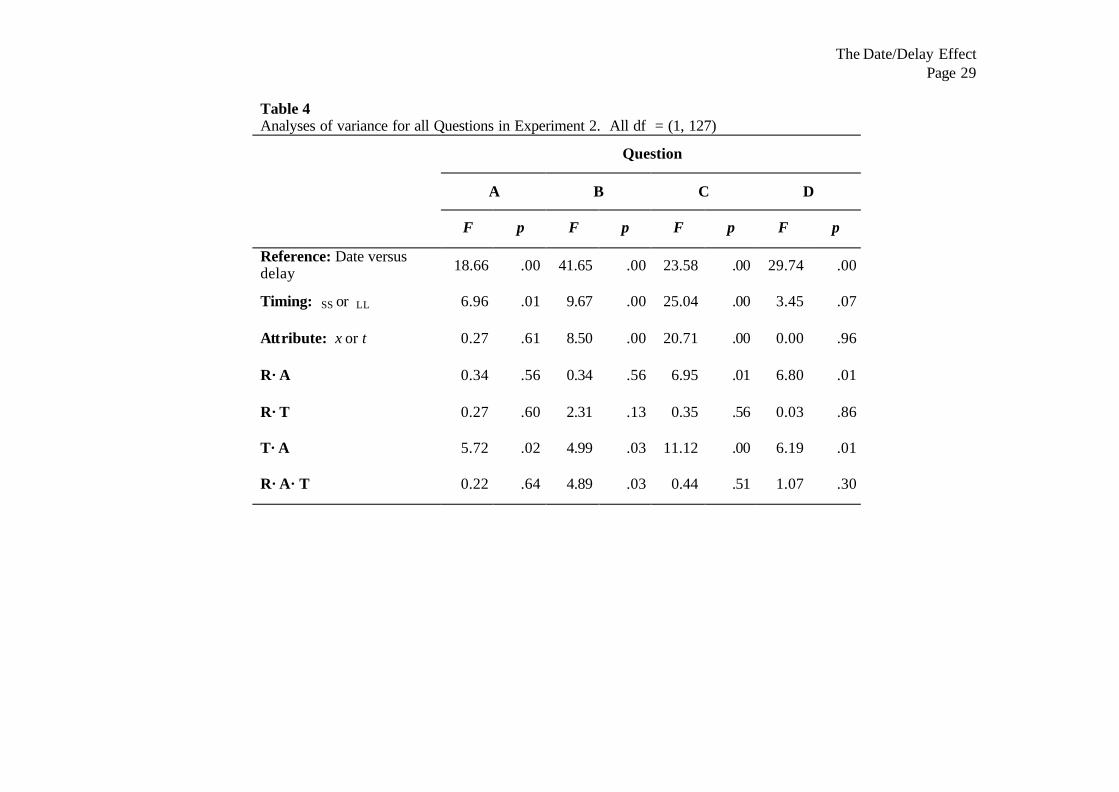
The mean values of δ, collapsed across all questions, are depicted in Figure 1.

We analysed the data by means of four 2×2×2 ANOVAs, one for each question, and

the results of these analyses are given in Table 4. We focus our discussion on the


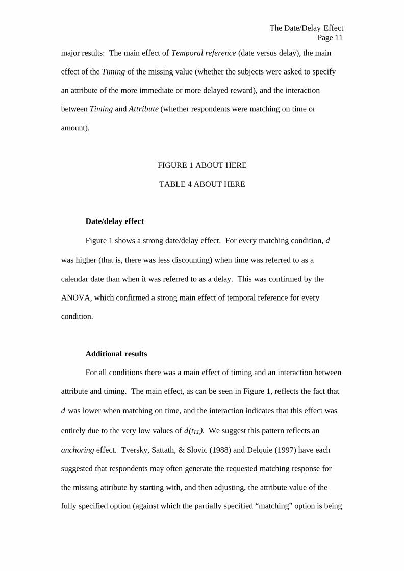
major results: The main effect of Temporal reference (date versus delay), the main

effect of the Timing of the missing value (whether the subjects were asked to specify

an attribute of the more immediate or more delayed reward), and the interaction

between Timing and Attribute (whether respondents were matching on time or

amount).

FIGURE 1 ABOUT HERE

TABLE 4 ABOUT HERE

Date/delay effect

Figure 1 shows a strong date/delay effect. For every matching condition, δ

was higher (that is, there was less discounting) when time was referred to as a

calendar date than when it was referred to as a delay. This was confirmed by the

ANOVA, which confirmed a strong main effect of temporal reference for every

condition.

Additional results

For all conditions there was a main effect of timing and an interaction between

attribute and timing. The main effect, as can be seen in Figure 1, reflects the fact that

δ was lower when matching on time, and the interaction indicates that this effect was

entirely due to the very low values of δ(tLL). We suggest this pattern reflects an

anchoring effect. Tversky, Sattath, & Slovic (1988) and Delquie (1997) have each

suggested that respondents may often generate the requested matching response for

the missing attribute by starting with, and then adjusting, the attribute value of the

fully specified option (against which the partially specified “matching” option is being


compared and, ostensibly, equated). In our stimuli, for example, a respondent asked

to provide xSS may start with xLL, and adjust that downward. To the extent that the

final response is “anchored on” or assimilated with the starting value, the adjustment

will be “insufficient” in the sense that an attribute will receive more weight when it is

the matching dimension than when it is the fully specified dimension (see Delquie,

1997). For our stimuli, this would increase δ when matching on amount (by

decreasing the difference between two amounts) and decrease δ when matching on

time (by decreasing the difference between two times). This can account for the main

effect of attribute. It does not, however, explain the the interaction (why the imputed

δ was lower when specifying the time of the later larger reward than when specifying

the time of the smaller sooner reward. One explanation, is that when matching on tLL

the standard anchoring story applies – people give a time close to tSS, thus decreasing

δ( tLL) -- but that when matching on tSS they anchor on the present t0 rather than on tLL.

This will increase the interval between the outcomes, thereby increasing δ and

producing the pattern observed in this study.

Experiment 3

Experiments 1 and 2 demonstrated the date/delay effect, and showed that

whatever distinguishes dates and delays is found in both matching and choice. We

now investigate what happens when both the date and delay perspectives are made

salient.

Method

Participants were 90 students from the LSE who were approached in the

library and courtyard and asked to complete our questionnaire.


The method was similar to that of Experiment 1. Participants chose between

pairs of outcomes where the times were referred to as either Delays in months, Dates,

or as Dates-plus-Delays, as shown below:

Option 1 Option 2

You receive: £900 £1200

When: In 4 months

Feb 27, 2004

In 20 months

June 24, 2003

The specific questions used in the experiment are summarised in Table 5.

TABLE 5 ABOUT HERE

For each participant, we obtained the proportion of times they chose LL. As

can be seen in Table 6, the pattern was clear. The Date condition yielded many more

choices of LL than the Delay condition, and the Date-and-Delay condition was much

closer to the Delay condition. An ANOVA on the average proportion choosing LL

indicated there were significant differences between the conditions, F(2,85)=4.29,

p<.02, and Tukey post-hoc tests showed that the Date condition differed from the

other two conditions, which did not differ from each other.

TABLE 6 ABOUT HERE

Thus, it appears that when both descriptions are presented concurrently people

choose as if they had seen the Delay description only. It leaves open the question of


how alternate temporal references interact when presented sequentially. If a

preference is first formed when a period is described by dates, will it be reversed

when a delay description is subsequently presented? If not, how durable is a

particular perspective? Presumably, not long, since all those people who showed such

large date/delay effects in these experiments would have, both frequently and

recently, been exposed to both types of descriptions.

Experiment 4

Hyperbolic discounting is the hypothesized tendency for the discount factor δ

to increase the farther in the future an outcome is expected to occur (Ainslie, 1975;

Strotz, 1955). Hyperbolic discounting predicts that for any pair of rewards separated

by a fixed interval (i.e., holding tLL– tSS constant), increasing the onset of that interval

(tSS) will increase the likelihood of choosing LL. Most tests of this prediction have

referred to time as a delay, and many of these have confirmed the prediction (e.g.,

Bleichrodt & Johannesson, 2001; Kirby & Herrnstein, 1995; Read & Roelofsma, 2003

Exp 1; Keren & Roelofsma, 1995 ; Van der Pol & Cairns, 2002 – though see

Ahlbrecht & Weber, 1997; Baron, 2000; Holcomb & Nelson, 1992; Read, 2001

Exp 2)3. On the other hand, in the few experiments describing time in terms of

calendar dates hyperbolic discounting has not been observed (Pender, 1996; Read,

2001; Read & Roelofsma, 2003 Experiment 2). This pattern of findings suggests

there may be a regularity, in which hyperbolic discounting occurs only (or, at least,

primarily) when time is referred to using delays. This hypothesis is tested in

Experiment 4.


Method

In this experiment, discounting was measured using a choice titration method,

as described in Read (2001). Participants chose between delayed options and, after

each choice, either xLL or xSS was adjusted until an indifference point was reached.

Participants were divided into four groups based on whether time was

described as a Date or Delay, and on whether the discounting period was Long or

Short. The stimuli are summarised in Table 6. The periods were divided into 4

intervals that spanned the interval from ti to ti+1. For example, in the Short condition

the first interval spanned the dates from August 30, 2002 to Nov 29, 2002 (1 month to

4 months), the second interval spanned the dates from Nov 29, 2002 to Feb 28, 2003

(4 months to 7 months), and so on. Hyperbolic discounting predicts that δ will

increase with interval onset.

TABLE 7 ABOUT HERE

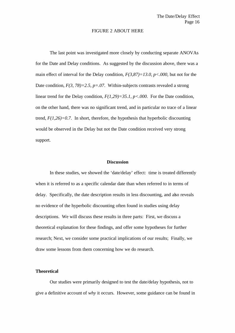
Results

The mean values of δ are depicted in Figure 2. As can be seen, δ was always

higher when time is referred to as a date than as a delay. Confirming this, there was a

significant main effect of time reference, F(1,55) = 5.6, p<.02. There was also a

main effect of interval, indicating that, consistent with the predictions of hyperbolic

discounting, δ increased for later interval onsets, F(3,165)=8.1, p<.000. However, as

can be seen in Figure 3, this increase was entirely due to the Delay condition, an

observation that is supported by the highly significant Interval by Time reference

interaction F(3,165)=9.4, p<.0001.


FIGURE 2 ABOUT HERE

The last point was investigated more closely by conducting separate ANOVAs

for the Date and Delay conditions. As suggested by the discussion above, there was a

main effect of interval for the Delay condition, F(3,87)=13.0, p<.000, but not for the

Date condition, F(3, 78)=2.5, p=.07. Within-subjects contrasts revealed a strong

linear trend for the Delay condition, F(1,29)=35.1, p<.000. For the Date condition,

on the other hand, there was no significant trend, and in particular no trace of a linear

trend, F(1,26)=0.7. In short, therefore, the hypothesis that hyperbolic discounting

would be observed in the Delay but not the Date condition received very strong

support.

Discussion

In these studies, we showed the ‘date/delay’ effect: time is treated differently

when it is referred to as a specific calendar date than when referred to in terms of

delay. Specifically, the date description results in less discounting, and also reveals

no evidence of the hyperbolic discounting often found in studies using delay

descriptions. We will discuss these results in three parts: First, we discuss a

theoretical explanation for these findings, and offer some hypotheses for further

research; Next, we consider some practical implications of our results; Finally, we

draw some lessons from them concerning how we do research.

Theoretical

Our studies were primarily designed to test the date/delay hypothesis, not to

give a definitive account of why it occurs. However, some guidance can be found in


recent articles suggesting that observed discounting behaviour is not determined by an

underlying discount function, but rather by similarity comparisons between options on

the dimensions of time and amount. Specifically, Leland (2002) and Rubinstein

(2000, 2003) propose that discounting over an interval is determined by the similarity

of the time-points marking its beginning and its end: the more similar, the less

discounting. Both authors stress the implications of their hypothesis for hyperbolic

discounting. Rubinstein argues that hyperbolic discounting occurs because the

similarity between two time-points separated by a common interval increases with the

onset of that interval: 12 months is more similar to 11 months than 2 months is to 1

month. The per-unit discount factor (δ), therefore, increases with interval onset. This

account easily fits the findings for the delay conditions of Experiment 4. If we extend

the similarity analysis to non-quantitative comparisons (implied, but not explicitly

discussed, by Rubinstein and Leland) it also fits the findings for the date conditions.

We suggest the similarity between dates separated by a common interval does not

change the later they occur. That is, the similarity of August 13, 2005 to September

22, 2005 is no greater than the similarity of August 13, 2004 to September 22, 2004.

Thus, we have hyperbolic discounting for delays, but not for dates.

Can the Rubinstein/Leland hypothesis also enlighten us about the greater

patience shown in the date condition? We suggest it can. Take as a single example

Question D from Experiment 1 (any question will do equally well): 3 months versus

16 months or August 29, 2003 versus September 24, 2004. If we use a

Rubinstein/Leland similarity metric, 3 and 16 months are pretty different, so we

should expect lots of discounting. For the date description, however, the story is

different. If we used a numerical metric, the dates are quite similar, and certainly

more similar than 3 versus 16: 29 is similar to 24; 2003 is similar to 2004. If we look


at the non-numerical months they are also similar -- August is adjacent to September

in the calendar. Indeed, most pairs of dates will be reasonably similar to one another,

and thus lead to relatively little discounting.

This perspective yields new hypotheses. For instance, the discounting

associated with dates might be influenced by the way in which they are presented.

For example, 8/29/03 might be less similar 9/24/04 than 8/29/2003 is to 9/24/2004

(because the ratio 2004/2003 is much less than 04/03); or August 1, 2003 might be

less similar to September 24, 2004 than July 24, 2003 is to September 24, 2004. We

leave these speculations, however, for future research, in which judgments of

similarity are elicited directly, rather than posited or inferred from responses to

intertemporal judgments.

Implications

The date/delay effect has important practical implications. One lesson is that

commercial retailers should refer to temporal outcomes in terms of calendar dates

when they want their clients to discount future outcomes very little (e.g. if the buyer

must incur unavoidable long shipping delays) and in terms of delays when they want

to encourage discounting (e.g. when the seller makes money from express shipping).

These implications may be greatest in the domain of investment and credit

offerings. When people think of the future in terms of calendar dates, they will be

more likely to invest and less likely to borrow, because there will be less discounting

over the interval between the present and the moment when future returns will be

received, or future payments must be made. For instance, when offering Bonds, Euro

Bills Treasury Bills, and other fixed term securities, it would be better to emphasize

the specific listed calendar date on which they mature, as this should reduce


discounting and increase willingness to invest at a given rate. Conversely, it may be

best to offer loans by referring to the delay until the loan comes due as this should

make future payments seem more distant, and therefore less onerous. In fact, this is

how Bonds and loans are advertised, although we doubt this is a strategic decision4.

Another implication is that ‘buy now, pay later…’ schemes should be more attractive

when described in delay terms (‘pay nothing for 6 months.’) than when described

using specific dates (‘pay nothing until June 2004’). An informal survey of retailers

in the UK making such offers found that the vast majority do, in fact, describe their

offerings in this way (though again we doubt that this is strategic).5

Governments could employ the date/delay effect to convey the attractiveness

of savings, and the unattractiveness of debt. It may be more effective to advertise

savings by marketing it as “If you put £1000 in a cash ISA [Individual Savings

Account] on the first day of 2004 it will be worth £1500 by Christmas, 2014,” than by

marketing it as “If you put £1000 in a cash ISA today it will be worth £1500 in less

than 11 years.” Likewise, to decrease consumer’s willingness to incur debt,

government regulation could require merchants to specify, in calendar terms, the

implications of loans, as in “… on January 28, 2004, February 27, 2004, and the last

Friday of every month thereafter until December 29, 2008, you must pay Johnson’s

Electronics $100.” Correspondingly, annuity products might seem more attractive

when payments are described as being made on a specific date each year.

Conclusion

Politicians and poets know that the quality and intensity of our responses to

acts or events is affected by how they are described. It should not surprise us,

therefore, that the way in which we refer to a temporal interval affects time


preference. Moreover, this finding is unlikely to be limited to the contrast between

date and delay descriptions, per se. For instance, dates that are “special” (e.g. may be

treated differently than other dates, particularly if the specialness is directly specified

(e.g. ‘on Christmas 2005,’ or ‘on your next birthday.’) Furthermore, there are still

other ways of referring to time, and each may be characterised by its own way of

discounting the future. For example, temporal events indexed by a person’s future

age could be discounted differently than those indexed in other ways: Someone who

is 35, might regard an outcome occurring 15 years away differently than one

occurring when they are 50, or one occurring in 2020. The perspective that

individuals spontaneously adopt think of the future, when no specific perspective is

cued, may even partly explain interindividual differences in discounting.

As a final note, our findings should also serve as a caution to researchers. As

discussed earlier, researchers usually choose temporal descriptions for arbitrary or

pragmatic reasons. Consequently, we, as researchers, often end up proposing as

general truths findings that apply only to the particular descriptions used in their

studies, a possibility given weight by the finding, in Experiment 4, that evidence for

hyperbolic discounting depends on temporal description. Perhaps we should be more

careful to follow the ‘operational approach’ advocated by Percy Bridgman (1927)

almost 80 years ago

If we have more than one set of operations [i.e., way of obtaining a result or

measuring a phenomenon], we have more than one concept, and strictly there

should be a separate name to correspond to each different set of operations. (p.

10).

When we measure effects in intertemporal choice, or in any other area of judgment

and decision making, we should be aware that those effects apply unambiguously only


to the specific set of operations we have chosen. Date-discounting and delay-

discounting are different concepts6, and the implications we draw from one kind of

discounting do not necessarily apply to the other.


References

Ahlbrecht, M., M.Weber. 1997. An empirical study on intertemporal decision making

under risk. Management Science 43(6) 813-826.

Ainslie, G. 1975. Specious reward: A behavioral theory of impulsiveness and impulse

control. Psychological Bulletin 82(4) 463-469.

Baron, J. 2000. Can we use human judgments to determine the discount rate? Risk

Analysis 20(6) 861-868.

Benzion, U., A. Rapoport, J. Yagil. 1989. Discount rates inferred from decisions - an

experimental-study. Management Science 35(3) 270-284.

Bleichrodt, H., & M. Johannesson. 2001. Time preference for health: A test of

stationarity versus decreasing timing aversion. Journal of Mathematical

Psychology 45(2) 265-282.

Bridgman, P. W. 1927. The logic of modern physics. New York.

Camerer, C. 1995. Individual decision making. J.H. Kagel, A.E. Roth, eds. The

Handbook of Experimental Economics. Princeton University Press, Princeton,

New Jersey 587-702.

Frederick, S., G. Loewenstein, T. O'Donoghue. 2002. Time discounting and time

preference: A critical review. Journal of Economic Literature 40(2) 351-401.

Frederick, S. & Shafir, E. 2004. Careless Choice and Mindless Matching: Elusive

Attribute Weights in Preference Elicitation” Working paper. Massachusetts

Institute of Technology.

Harless, D. W. 1992. Actions versus prospects: The effect of problem representation

on regret. American Economic Review 82(3) 634-649.

Holcomb, J. H., & P. S. Nelson. 1992. Another experimental look at individual time

preference. Rationality and Society 4(2) 199-220.


Kahneman D., & A. Tversky. 1984. Choices, values and frames. American

Psychologist 39(4) 341-350.

Keren, G., & P.H.M.P. Roelofsma. 1995. Immediacy and certainty in intertemporal

choice. Organizational Behavior and Human Decision Processes 63(3) 287-

297.

Kirby, K. N. 1997. Bidding on the future: Evidence against normative discounting of

delayed rewards. Journal of Experimental Psychology - General 126(1) 54-70.

Laibson, D. I. 2002. Intertemporal decision making. URL: http://

post.economics.Harvard.edu/faculty/laibson/papers/ecsmar2.pdf.

Leland, J. W. 2002. Similarity judgments and anomalies in intertemporal choice.

Economic Inquiry 40(4) 574-581.

Loewenstein, G. F. 1988. Frames of mind in intertemporal choice. Management

Science 34(2) 200-214.

Pender, J. L. 1996. Discount rates and credit markets: Theory and evidence from rural

India. Journal of Development Economics 50(2) 257-96.

Read, D. 2001. Is time-discounting hyperbolic or subadditive? Journal of Risk and

Uncertainty 23(1) 5-32.

Read, D., & P.H.M.P. Roelofsma. 2003. Subadditive versus hyperbolic discounting:

A comparison of choice and matching. Organizational Behavior and Human

Decision Processes 91(2) 140-153.

Read, D. 2004. Intertemporal choice. D. Koehler, N. Harvey, eds. Blackwell

Handbook of Judgment and Decision Making Oxford: Blackwell.

Rubinstein, A. 2000. Is it Economics and Psychology? The Case of Hyperbolic

Discounting. Working paper, University of Tel Aviv/Princeton University.


Rubinstein, A. 2003. “Economics and Psychology"? The Case of Hyperbolic

Discounting. International Economic Review 44(4) 1207-1216.

Starmer, C., R., & Sugden. 1993. Testing for juxtaposition and event –splitting

effects. Journal of Risk and Uncertainty 6(3) 235-254.

Strotz, R.H. 1955. Myopia and inconsistency in dynamic utility maximization. Review

of Economic Studies 23(3) 165-180.

Thaler, R. 1981. Some empirical evidence of dynamic inconsistency. Economics

Letters 8(3) 201-207.

Tversky, A., S., Sattath, P. Slovic. 1988. Contingent weighting in judgment and

choice. Psychological Review 95(3) 371-384.

Van der Pol, M., & J. Cairns. 2002. A comparison of the discounted utility model and

hyperbolic discounting models in the case of social and private intertemporal

preferences for health. Journal of Economic Behavior & Organization 49(1)

79-96.


Endnotes

1 It must be emphasised that Strotz was not explicitly making a claim about temporal

description, but only about the two factors that go into time discounting.

Inadvertently, he described a significant phenomenon.

2 Questionnaires were not used if they were incomplete, or if they had at least one

response implying a negative discount rate, or an uninterpretable response.

Uninterpretable responses were those in which words were used in place of numbers,

times were filled-in when amounts were required, or vice-versa.

3 Note that this list excludes a large number of studies in which interval length was not

held constant.

4 There are good reasons for the two kinds of presentation that have nothing to do with

the date/delay effect. A Euro bill offering is put on the market on one day, and

matures on a specific day, and so it is natural – and legally required – to describe the

offering in terms of dates. On the other hand, consumer loans are flexible instruments

that vary both in the time when they become available, and the repayment term.

Again, it is natural to describe the terms in more abstract ‘delay’ terms. 5 There was one curious exception. When this passage was first written in December

2003) several retailers were offering ‘Buy now, pay nothing until 2005’ credit, which

is somewhere between date and delay. But 2005 was barely more than 12 months

away (and payments are to start in January 2005), and we suspect people will perceive

the difference between 2003 and 2005 as greater than 12 months. Within a few

weeks, in January 2004, the offer had changed to ‘Buy now, pay nothing for 12

months.’

6 Later, Bridgman asserts about two kinds of measurement: ‘The practical

justification for retaining the same name is that within our present experimental limits

a numerical difference between the results of the two sorts of operations has not been

detected. (p. 16)’


Table 1

Amounts and times used in Experiment 1.

Question A B C D SS LL SS LL SS LL SS LL Amount(£) 370 450 520 740 770 1480 900 1200

Date Sept 26,

2003 June 25,

2004 July 25,

2003 Nov 26,

2004 Nov 28,

2003 May 26,

2006 Aug 29,

2003 Sept 24,

2004 Months 4 13 2 18 6 36 3 16 Weeks 17 56 9 78 26 156 13 65


Table 2 Percent choosing the later (LL) amount given different descriptions of time period in Experiment 1

Description

Question Date Month Week

A 60 29 14

B 63 18 07

C 60 43 32

D 53 18 21

Mean 591 272 192

N 30 28 28

Numbers in a row with a common superscript do not differ significantly by Tukey HSD test.


Table 3 Amounts and times used in Experiment 2.

Question

A B C D

SS LL SS LL SS LL SS LL

Amount in £ 370 450 520 740 70 1480 900 1200

Date Oct 31, 2003

July 7, 2004

Aug 29, 2003

Dec 31, 2004

Dec 26, 2003

June 30, 2006

Sept 26, 2003

Oct 29, 2004

Delay (months) 4 13 2 18 6 36 3 16


Table 4 Analyses of variance for all Questions in Experiment 2. All df = (1, 127)

Question

A B C D

F p F p F p F p

Reference: Date versus delay 18.66 .00 41.65 .00 23.58 .00 29.74 .00

Timing: ⋅SS or ⋅LL 6.96 .01 9.67 .00 25.04 .00 3.45 .07

Attribute: x or t 0.27 .61 8.50 .00 20.71 .00 0.00 .96

R×A 0.34 .56 0.34 .56 6.95 .01 6.80 .01

R×T 0.27 .60 2.31 .13 0.35 .56 0.03 .86

T×A 5.72 .02 4.99 .03 11.12 .00 6.19 .01

R×A×T 0.22 .64 4.89 .03 0.44 .51 1.07 .30


Table 5 Amounts and times used in Experiment 3.

Question

A B C D

SS LL SS LL SS LL SS LL

Amount (£) 900 1200 750 2000 520 780 465 870

Date Feb 27,

2004 June 24,

2005 April

30, 2004 Oct 31, 2008

Dec 26, 2003

Oct 28, 2005

Mar 26, 2004

Feb 23, 2007

Delay (month) 4 20 6 60 2 24 5 40


Table 6 Percent choosing the later (LL) amount given different descriptions of time period in Experiment 3

Description

Question Date Month Date-plus-month

A 47 18 23

B 50 25 33

C 33 21 13

D 30 11 13

Mean 401 192 212

N 28 30 30

Numbers with a common superscript do not differ significantly by Tukey HSD test.


Table 7 Dates, delays and interval lengths in all conditions of Experiment 4 Time points

Interval Reference t1 t2 t3 t4 t5

Date Aug 30, 2002 Nov 29, 2002 Feb 28, 2003 May 30, 2003 Aug 29, 2003 Short

Delay In 1 month In 4 months In 7 months In 10 months In 13 months

Date Oct 25, 2002 Aug 29, 2003 April 30, 2004 Jan 28, 2005 Oct 28, 2005 Long

Delay In 3 months In 12 months In 21 months In 30 months In 39 months


Figure 1 Results of Experiment 2, showing effect of Date and Delay when matching on both amount (xS and xL) and time (tS and tL).

0.2

0.3

0.4

0.5

0.6

0.7

0.8

Date Delay

δd(tSS)d(tLL)d(xSS)d(xLL)


Figure 2: Results of Experiment 4, showing effect of Date and Delay.

Short intervals

0.4

0.5

0.6

0.7

0.8

1 2 3 4

Interval

DelayDate

δ

Long intervals

0.4

0.5

0.6

0.7

0.8

1 2 3 4

Interval

DelayDate

δ

four score and seven years from now: the …eprints.lse.ac.uk/22749/1/04065.pdf · four score and...

Documents