four essays on macroprudential policy and cross-border · pdf filethis thesis was written...
TRANSCRIPT

ANNÉE 2014
THÈSE / UNIVERSITÉ DE RENNES 1sous le sceau de l’Université Européenne de Bretagne
pour le grade de
DOCTEUR DE L’UNIVERSITÉ DE RENNES 1
Mention : Sciences Économiques
École doctorale Sciences de l’Homme des Organisationset de la Société (SHOS)
présentée par
Gauthier Vermandelpréparée à l’unité de recherche CREM (UMR6211)Centre de Recherche en Economie et Management
Faculté de Sciences Économiques
Essays oncross-border bankingand macroprudentialpolicy.
Thèse soutenue à Rennesle 3 Décembre 2014devant le jury composé de :
Jean-Bernard ChatelainProfesseur, IUF, Université Paris 1 Panthéon-SorbonneRapporteur
Patrick FèveProfesseur, École d’Économie de ToulouseRapporteur
Rafael WoutersAdvisor, Banque Nationale de BelgiqueRapporteur
Laurent ClercDirecteur de la Stabilité Financière, Banque de FranceExaminateur
Marc-Alexandre SénégasProfesseur, Université de BordeauxPrésident de Jury
Samuel MaveyraudMaître de Conférences, HDR, Université de BordeauxCo-directeur
Jean-Christophe PoutineauProfesseur, Université de Rennes 1Directeur


This Ph.D. thesis should not be reported as representing the views of University of
Rennes 1. The views expressed are those of the author and do not necessarily reflect
those of the University.
L’Universite de Rennes 1 n’entend donner aucune approbation ni improbation aux opin-
ions emises dans cette these. Ces opinions doivent etre considerees comme propres a
leur auteur.


“To mitigate potential negative cross-border spillovers, national and European [macro-
prudential] authorities must work together to assess ex ante the effects of planned ac-
tions at the level of the institution, the country, the region and the Union as a whole.
Authorities should strive to minimise potential negative cross-border spillovers and to
communicate coherently and in unison.”
Mario Draghi, Chair of the ESRB
ESRB introductory statement, Brussels, 16 January 2012.


Acknowledgements
This Ph.D. dissertation, hosted and financed by the University of Rennes 1, is the result
of effort of many people, from the University of Bordeaux where I started my Ph.D. in
the first year, to the University of Rennes in the second year and finally at the ECB in
Frankfurt for my last year.
I would like to express my gratitude to my advisors Jean-Christophe Poutineau and
Samuel Maveyraud for their immeasurable support and encouragement. I am also in-
debted to the members of my dissertation committee for giving me the honor of par-
ticipating to my Ph.D. defense: Jean-Bernard Chatelain, Patrick Feve, Rafael Wouters,
Laurent Clerc and Marc-Alexandre Senegas.
This thesis was written while I was working as a Ph.D. intern at the European Central
Bank, DG-Macro-Prudential Policy and Financial Stability, Macro-Financial Linkages
Division in 2014. I thank my team division for their kindness, especially my Head of
Division Jerome Henry. I was in the perfect place with amazing conditions to work on
Macroprudential Policy for the Euro Area. I also thank Christoffer Kok and Matthieu
Darracq-Paries for giving me this opportunity to co-work on an extension of their well-
known DKR model with some ingredients from my thesis.
I also thank my office colleagues and friends at the ECB for the good moments during
the writing of my thesis dissertation, in particular Anil Ari, Codruta Boar, Thibaut
Duprey, Daniel-Oliver Garcia Macia, Sophia List, Despo Malikkidou, Madalina Minu,
Andreea Piloiu, Alexandra Popescu, Sandra Rhouma, Yves S. Schueler and Jonathan
Smith.
I’m also indebted to Miguel Casares for sharing his Matlab codes, recommending me
and encouraging me since the very beginning of my thesis. Also, I would like to thank
Ivan Jaccard for his helpful advices since we met at a CEPR event.
Most of these thesis chapters were presented in workshops and conferences. At these
occasions, I thank the seminar participants for helpful comments and suggestions, in par-
ticular Jean-Pierre Allegret, Cristina Badarau, Sophie Bereau, Frederic Boissay, Camille
Cornand, Luca Fornaro, Robert Kollmann, Dimitris Korobilis, Olivier L’haridon, Gregory
Levieuge, Fabien Moizeau, Manuel Mota Freitas Martins, Tovonony Razafindrabe, Marco
Ratto, Dominik M. Rosch, Katheryn Russ and Karl Walentin.
Finally, I also thank the editor and one of the associate editors of the Journal of Eco-
nomic Dynamics and Control as well as six anonymous referees in different peer-review
journals for their constructive remarks on three chapters of this thesis which resulted in
publications.
vii


Remerciements
Ces trois annees de these auront ete passionnantes et enrichissantes. J’ai eu la chance
d’avoir ete heberge par trois institutions differentes ou les echanges avec leurs membres
m’ont enormement apporte.
Tout d’abord, je tiens a remercier mes directeurs de these pour ce qu’ils m’ont apporte
depuis le debut, parfois dans les moments difficiles. Leurs attentions, leurs encourage-
ments a mon egard m’ont conduit a poursuivre ma these sans jamais douter. J’ai une
pensee toute particuliere pour Jean-Christophe Poutineau, dont l’exigence m’a conduit
a repousser les limites que je croyais infranchissables.
Je remercie egalement l’Universite de Rennes 1 et plus particulierement le CREM, ou
j’ai pu beneficier de conditions de travail excellentes au sein d’une unite de recherche
tres dynamique. Je remercie son directeur, Yvon Rocaboy. Le personnel de cette unite
de recherche est exceptionnel, je remercie Anne L’Azou, Helene Coda-Poirey et Julie Le
Diraison pour leur reactivite et leur aide.
Je revais de faire des etudes en informatique ou en statistiques, je termine en doctorat
d’economie. Je suis reconnaissant a ceux qui m’ont devie de ma trajectoire initiale dans
mes premieres annees a l’Universite de Bordeaux. Je pense en particulier a Bertrand
Blancheton et Samuel Maveyraud qui, des ma premiere annee de licence, m’ont en-
courage et oriente vers le Master puis le Doctorat. Je remercie Marc-Alexandre Senegas
pour son soutien lors de ma premiere annee de these malgre ses contraintes personnelles.
Je remercie egalement Henri Bourguinat, Murat Yildizoglu et Marie Lebreton pour leurs
soutiens et encouragements.
Je remercie egalement les doctorants rennais et bordelais avec qui j’ai partage ces annees
de these. Je pense a Laurent Baratin, Thibaut Cargoet, Leo Charles, Ewen Gallic,
Pauline Lectard, Laisa Roi, Isabelle Salle, Pascaline Vincent ainsi que tous les membres
de l’association rennaise PROJECT pour tous ces incroyables moments partages. J’ai
une pensee pour Pauline et Laurent, avec qui j’ai traverse la galere d’une annee sans
financement a Bordeaux, nous etions surcharges d’enseignement et sans bureau. Je pense
a eux qui sont toujours dans cette situation et leur temoigne toute mon admiration dans
leur determination a poursuivre un doctorat.
Je pense a ma famille, mes petits freres, mes parents et mes proches, qui m’ont supporte
durant cette aventure academique. Je les remercie pour tout ce qu’ils m’ont apporte en
depit de mon eloignement geographique, ils ont toujours ete la pour m’aider quand j’en
avais besoin.
ix

Enfin, je remercie une derniere fois mes directeurs de these pour la relecture de la these,
ainsi que Thibaut Cargoet, Ewen Gallic, Jeremy Rastouil et Fabien Rondeau.

Contents
Acknowledgements vii
Remerciements ix
Contents xi
General Introduction 1
1 Towards a New Normality in Economic Policy . . . . . . . . . . . . . . . 1
2 The Recent Evolution of DSGE Models . . . . . . . . . . . . . . . . . . 4
3 European Features . . . . . . . . . . . . . . . . . . . . . . . . . . . . . . 6
4 Key Contributions of the Thesis . . . . . . . . . . . . . . . . . . . . . . 10
5 Structure of the Thesis . . . . . . . . . . . . . . . . . . . . . . . . . . . . 12
1 An Introduction to Macroprudential Policy 17
1 Introduction . . . . . . . . . . . . . . . . . . . . . . . . . . . . . . . . . . 17
2 The effect of financial frictions in the case of a simple monetary policy rule 20
2.1 A Static New Keynesian Model with a Banking System . . . . . 20
2.2 The Consequences of the Procyclicality of the Financial System . 23
3 Optimal Monetary Policy and the Concern for Financial Stability . . . . 25
3.1 The Optimal Monetary Policy without a Financial Stability Concern 26
3.2 The Optimal Monetary Policy with a Financial Stability Concern 27
4 Macroprudential Policy . . . . . . . . . . . . . . . . . . . . . . . . . . . 28
4.1 The Nature of Macroprudential Policy . . . . . . . . . . . . . . . 29
4.2 The Design of Macroprudential Policy . . . . . . . . . . . . . . . 30
4.2.1 The Nash equilibrium . . . . . . . . . . . . . . . . . . . 32
4.2.2 The cooperative equilibrium . . . . . . . . . . . . . . . 34
5 Conclusion . . . . . . . . . . . . . . . . . . . . . . . . . . . . . . . . . . 36
2 Cross-border Corporate Loans and International Business Cycles in aMonetary Union 39
1 Introduction . . . . . . . . . . . . . . . . . . . . . . . . . . . . . . . . . . 39
2 Une union monetaire avec prets transfrontaliers . . . . . . . . . . . . . 41
2.1 Choix d’investissement et flux bancaires transfrontaliers . . . . . 41
2.2 Le reste du modele . . . . . . . . . . . . . . . . . . . . . . . . . . 44
2.2.1 Les menages . . . . . . . . . . . . . . . . . . . . . . . . 44
2.2.2 Les syndicats . . . . . . . . . . . . . . . . . . . . . . . . 45
xi

Contents
2.2.3 Les entreprises . . . . . . . . . . . . . . . . . . . . . . . 46
2.2.4 Le producteur de biens capitaux . . . . . . . . . . . . . 47
2.2.5 Le secteur bancaire . . . . . . . . . . . . . . . . . . . . 48
2.3 Les autorites . . . . . . . . . . . . . . . . . . . . . . . . . . . . . 50
2.4 Equilibre General . . . . . . . . . . . . . . . . . . . . . . . . . . . 50
3 Estimation des parametres du modele . . . . . . . . . . . . . . . . . . . 51
4 Effets macroeconomiques des prets transfrontaliers . . . . . . . . . . . . 55
4.1 Les consequences de chocs reel et financier asymetriques . . . . . 55
4.2 La decomposition de la variance . . . . . . . . . . . . . . . . . . 58
5 Conclusion . . . . . . . . . . . . . . . . . . . . . . . . . . . . . . . . . . 59
3 Macroprudential Policy with Cross-border Corporate Loans: Granu-larity Matters 61
1 Introduction . . . . . . . . . . . . . . . . . . . . . . . . . . . . . . . . . . 61
2 Relation to the literature . . . . . . . . . . . . . . . . . . . . . . . . . . 64
3 Cross-Border Bank Loans and the Macroprudential Setting . . . . . . . 65
3.1 Entrepreneurs and the Demand for Loans . . . . . . . . . . . . . 66
3.2 The Banking Sector and the Imperfect Pass-Through of Policy Rate 69
3.2.1 Loan supply decisions . . . . . . . . . . . . . . . . . . . 70
3.2.2 Deposit supply decisions . . . . . . . . . . . . . . . . . 71
3.3 Macroprudential Policy . . . . . . . . . . . . . . . . . . . . . . . 71
4 The rest of the model . . . . . . . . . . . . . . . . . . . . . . . . . . . . 73
4.1 Households . . . . . . . . . . . . . . . . . . . . . . . . . . . . . . 74
4.2 Firms . . . . . . . . . . . . . . . . . . . . . . . . . . . . . . . . . 75
4.3 Monetary Policy . . . . . . . . . . . . . . . . . . . . . . . . . . . 76
4.4 Capital Suppliers . . . . . . . . . . . . . . . . . . . . . . . . . . . 76
4.5 Governments . . . . . . . . . . . . . . . . . . . . . . . . . . . . . 77
4.6 Aggregation and Market Equilibrium. . . . . . . . . . . . . . . . . . . . . . . . . . . . . . . . . . . . 77
4.6.1 Goods Market . . . . . . . . . . . . . . . . . . . . . . . 78
4.6.2 Loan Market . . . . . . . . . . . . . . . . . . . . . . . . 79
4.6.3 Deposit Market . . . . . . . . . . . . . . . . . . . . . . 79
5 Estimation . . . . . . . . . . . . . . . . . . . . . . . . . . . . . . . . . . 79
5.1 Data . . . . . . . . . . . . . . . . . . . . . . . . . . . . . . . . . . 79
5.2 Calibration and Priors . . . . . . . . . . . . . . . . . . . . . . . . 80
5.3 Posteriors and Fit of the model . . . . . . . . . . . . . . . . . . . 82
6.1 The Welfare Performance of Alternative Macroprudential Schemes 87
The Welfare Performance of Alternative Macroprudential Schemes . . . 87
The Welfare Performance of Alternative Macroprudential Schemes . . . 87
6 The Ranking of Alternative Macroprudential Schemes . . . . . . . . . . 87
The Welfare Performance of Alternative Macroprudential Schemes . . . 87
6.2 Macroeconomic Performances . . . . . . . . . . . . . . . . . . . . 92
6.3 The critical role of cross-border loans . . . . . . . . . . . . . . . 92
7 The Impact of Macroprudential Policies: a counterfactual analysis . . . 93
7.1 The preventive impact of a macroprudential policy . . . . . . . . 93
7.2 The curative impact of a macroprudential policy . . . . . . . . . 95
8 Conclusion . . . . . . . . . . . . . . . . . . . . . . . . . . . . . . . . . . 97

Contents
4 Cross-border Interbank Loans and International Spillovers in a Mon-etary Union 99
1 Introduction . . . . . . . . . . . . . . . . . . . . . . . . . . . . . . . . . . 99
2 Stylized Facts and Related Literature . . . . . . . . . . . . . . . . . . . 101
2.1 Cross-border lending in the Eurozone . . . . . . . . . . . . . . . 101
2.2 A quick summary of the related literature . . . . . . . . . . . . . 103
3 A Monetary Union with Cross-border Loans . . . . . . . . . . . . . . . 105
3.1 An Heterogenous Banking System . . . . . . . . . . . . . . . . . 106
3.1.1 Illiquid Banks . . . . . . . . . . . . . . . . . . . . . . . 106
3.1.2 Liquid Banks . . . . . . . . . . . . . . . . . . . . . . . . 108
3.2 Entrepreneurs and Corporate loans . . . . . . . . . . . . . . . . . 111
4 The Rest of the Model . . . . . . . . . . . . . . . . . . . . . . . . . . . . 113
4.1 Households . . . . . . . . . . . . . . . . . . . . . . . . . . . . . . 113
4.2 Labor Unions . . . . . . . . . . . . . . . . . . . . . . . . . . . . . 114
4.3 Firms . . . . . . . . . . . . . . . . . . . . . . . . . . . . . . . . . 115
4.4 Capital Suppliers . . . . . . . . . . . . . . . . . . . . . . . . . . . 116
4.5 Authorities . . . . . . . . . . . . . . . . . . . . . . . . . . . . . . 117
4.6 Equilibrium conditions . . . . . . . . . . . . . . . . . . . . . . . . 118
5 Estimation . . . . . . . . . . . . . . . . . . . . . . . . . . . . . . . . . . 120
5.1 Data . . . . . . . . . . . . . . . . . . . . . . . . . . . . . . . . . . 120
5.2 Calibration and Prior Distribution of Parameters . . . . . . . . . 120
5.3 Posterior Estimates . . . . . . . . . . . . . . . . . . . . . . . . . 123
6 The Consequences of Cross-border Loans . . . . . . . . . . . . . . . . . 127
6.1 A Positive Shock on Total Factor Productivity . . . . . . . . . . 127
6.2 A Negative Shock on Firms Net Worth . . . . . . . . . . . . . . . 130
6.3 A Positive Shock on Bank Resources . . . . . . . . . . . . . . . . 131
7 The Driving Forces of Business and Credit Cycles . . . . . . . . . . . . . 133
7.1 The Historical Variance Decomposition . . . . . . . . . . . . . . 133
7.2 Understanding the Time Path of the Current Account . . . . . . 135
7.3 Counterfactual Analysis . . . . . . . . . . . . . . . . . . . . . . . 138
8 Conclusion . . . . . . . . . . . . . . . . . . . . . . . . . . . . . . . . . . 139
5 Combining National Macroprudential Measures with Cross-border In-terbank Loans in a Monetary Union 143
1 Introduction . . . . . . . . . . . . . . . . . . . . . . . . . . . . . . . . . . 143
2 The Institutional Background . . . . . . . . . . . . . . . . . . . . . . . . 145
2.1 The Federal Organization of Macroprudential Policy . . . . . . . 145
2.2 The granular implementation of macroprudential measures . . . 146
3 The Analytical Framework . . . . . . . . . . . . . . . . . . . . . . . . . . 148
Households . . . . . . . . . . . . . . . . . . . . . . . . . . 149
Firms . . . . . . . . . . . . . . . . . . . . . . . . . . . . . 150
Entrepreneurs . . . . . . . . . . . . . . . . . . . . . . . . . 150
Banks . . . . . . . . . . . . . . . . . . . . . . . . . . . . . 151
Capital Suppliers . . . . . . . . . . . . . . . . . . . . . . . 152
Monetary Policy . . . . . . . . . . . . . . . . . . . . . . . 152
Shocks and Equilibrium Conditions . . . . . . . . . . . . . 152
4 Estimation and Empirical Performance . . . . . . . . . . . . . . . . . . . 153

Contents
4.1 Data . . . . . . . . . . . . . . . . . . . . . . . . . . . . . . . . . . 153
4.2 Calibration and Priors . . . . . . . . . . . . . . . . . . . . . . . . 154
4.3 Posteriors and Fit of the model . . . . . . . . . . . . . . . . . . . 159
5 Macroprudential Policy . . . . . . . . . . . . . . . . . . . . . . . . . . . 161
5.1 Countercyclical Capital Buffers . . . . . . . . . . . . . . . . . . . 161
5.2 Loan-to-Income Ratio . . . . . . . . . . . . . . . . . . . . . . . . 163
6 The setting of instruments . . . . . . . . . . . . . . . . . . . . . . . . . . 164
6.1 Setting individual instruments . . . . . . . . . . . . . . . . . . . 165
6.2 Combining multiple instruments . . . . . . . . . . . . . . . . . . 166
6.3 Macroeconomic performances . . . . . . . . . . . . . . . . . . . . 170
7 Sensitivity Analysis . . . . . . . . . . . . . . . . . . . . . . . . . . . . . . 171
8 Conclusion . . . . . . . . . . . . . . . . . . . . . . . . . . . . . . . . . . 172
General Conclusion 175
A The Non-Linear Model Derivations 177
1 The Non-Linear Model . . . . . . . . . . . . . . . . . . . . . . . . . . . . 178
1.1 The households utility maximization problem . . . . . . . . . . . 179
1.2 Labor Unions . . . . . . . . . . . . . . . . . . . . . . . . . . . . . 180
1.3 The Final Goods Sector . . . . . . . . . . . . . . . . . . . . . . . 181
1.4 The Intermediate Goods Sector . . . . . . . . . . . . . . . . . . . 183
1.5 Entrepreneurs . . . . . . . . . . . . . . . . . . . . . . . . . . . . . 184
1.5.1 The Balance Sheet . . . . . . . . . . . . . . . . . . . . . 185
1.5.2 The Distribution of Risky Investment Projects . . . . . 185
1.5.3 Profit Maximization and the Financial Accelerator . . . 189
1.6 Capital Goods Producers . . . . . . . . . . . . . . . . . . . . . . 190
1.6.1 Capital Supply Decisions . . . . . . . . . . . . . . . . . 190
1.6.2 The Rentability of one Unit of Capital . . . . . . . . . 193
1.6.3 Capital Utilization Decisions . . . . . . . . . . . . . . . 193
1.7 The Banking Sector . . . . . . . . . . . . . . . . . . . . . . . . . 195
1.7.1 The Financial Intermediary (CES Packer) . . . . . . . . 195
1.7.2 The Commercial Bank . . . . . . . . . . . . . . . . . . 197
Illiquid Banks . . . . . . . . . . . . . . . . . . . . . . . . . 198
Liquid Banks . . . . . . . . . . . . . . . . . . . . . . . . . 201
The loan supply decisions . . . . . . . . . . . . . . . . . . 202
The deposit decisions . . . . . . . . . . . . . . . . . . . . . 203
1.8 Authorities . . . . . . . . . . . . . . . . . . . . . . . . . . . . . . 205
1.9 Aggregation and Market Equilibrium. . . . . . . . . . . . . . . . . . . . . . . . . . . . . . . . . . . . 207
1.9.1 Goods Market . . . . . . . . . . . . . . . . . . . . . . . 207
1.9.2 Loan Market . . . . . . . . . . . . . . . . . . . . . . . . 209
1.9.3 Interbank Market . . . . . . . . . . . . . . . . . . . . . 210
1.9.4 Deposit Market . . . . . . . . . . . . . . . . . . . . . . 210
2 Definitions for Higher-Order Approximations . . . . . . . . . . . . . . . 211
2.1 The welfare index . . . . . . . . . . . . . . . . . . . . . . . . . . 211
2.2 New Keynesian Phillips curves in a recursive fashion . . . . . . . 213

Contents
2.2.1 Sticky Price . . . . . . . . . . . . . . . . . . . . . . . . 213
2.3 Sticky Wage . . . . . . . . . . . . . . . . . . . . . . . . . . . . . . 214
2.3.1 Sticky Credit Rate . . . . . . . . . . . . . . . . . . . . . 215
2.3.2 Sticky Deposit Rate . . . . . . . . . . . . . . . . . . . . 216
B The Linear Model 217
1 Households . . . . . . . . . . . . . . . . . . . . . . . . . . . . . . . . . . 217
2 Unions . . . . . . . . . . . . . . . . . . . . . . . . . . . . . . . . . . . . . 217
3 Firms . . . . . . . . . . . . . . . . . . . . . . . . . . . . . . . . . . . . . 218
4 Entrepreneurs . . . . . . . . . . . . . . . . . . . . . . . . . . . . . . . . . 218
5 Banks . . . . . . . . . . . . . . . . . . . . . . . . . . . . . . . . . . . . . 219
6 Capital Supply Decisions . . . . . . . . . . . . . . . . . . . . . . . . . . . 220
7 International Macroeconomics Definitions . . . . . . . . . . . . . . . . . 220
8 Monetary Policy . . . . . . . . . . . . . . . . . . . . . . . . . . . . . . . 221
9 Shocks Processes . . . . . . . . . . . . . . . . . . . . . . . . . . . . . . . 221
C Additional Quantitative Results 223
1 Empirical Performances . . . . . . . . . . . . . . . . . . . . . . . . . . . 223
2 Driving Forces of Output . . . . . . . . . . . . . . . . . . . . . . . . . . 225
3 Robustness Check to the Zero Lower Bound . . . . . . . . . . . . . . . . 227
4 Historical Decomposition of Business and Credit Cycles in the UEM . . 229
References 233
List of Figures 233
List of Tables 237


General Introduction
The aim of this thesis is to evaluate the conduct of macroprudential policies in an
heterogeneous monetary union, such as the Eurozone, by borrowing on the recent theo-
retical and empirical developments of Dynamic Stochastic General Equilibrium (DSGE)
models.
This introduction briefly sketches the main building blocks of this thesis. Section 1
quickly summarizes the consequences of the recent financial crisis on the conduct of
economic policy in developed economies, by insisting more particularly on the intro-
duction of macroprudential concerns. Section 2 outlines some useful recent theoretical
and econometric progresses made by DSGE models to account for financial factors in
the determination of economic equilibrium and to provide the basis for the modeling of
macroprudential policies. Section 3 presents some main Eurozone economic and insti-
tutional specificities that we consider to be important in the building of our analytical
framework. Section 4 provides a survey of the main contributions of the thesis to the
existing literature. Section 5 describes the structure of the thesis, organized in 5 chap-
ters.
1 Towards a New Normality in Economic Policy
Over the two decades preceding the subprime crisis of 2007, a widespread consensus
identified low and stable inflation as the primary mandate of monetary policy to pro-
vide macroeconomic stability. The general agreement among macroeconomists was that
the decline in the variability of output and inflation (”the great moderation”) observed
in the data could be linked to a coherent policy framework based upon the conduct of
monetary policy using an interest rate aimed at stabilizing inflation. Controlling infla-
tion would in turn limit the output gap. In the meanwhile, mainstream macroeconomics
had taken a benign view on financial factors in amplifying output and employment fluc-
tuations. In this policy environment, the stability of the financial system was achieved
through microprudential regulation insuring the soundness and safety of individual fi-
nancial institutions.
1

2 GENERAL INTRODUCTION
Ignoring the macroeconomic implications of financial imbalances that affected the Eu-
rozone (Figure 1) proved to be extremely costly. The consequences of the US sub-prime
crisis of 2007 and the accompanying dramatic fall in output (Figure 2) and rise in
unemployment exposed the limitations of the economic framework that was successful
in providing macroeconomic stability during the ”great moderation” period.
2004 2006 2008 2010 2012
600
700
800
900
(a) Corporate Loans
2004 2006 2008 2010 2012
160
180
200
220
(b) Real Estate Loans
2004 2006 2008 2010 2012
700
800
900
1 000
(c) Interbank Loans
Time Serie 1999-2014 Linear TrendExcessive Growth Losses
Figure 1: Boom and bust cycles in the Eurozone (millions of euro per capita, sourcesECB).
2005 2010
14 000
15 000
16 000
17 000
(a) Euro Area(Billion euros)
2005 2010
14 000
16 000
18 000
(b) The United States(Billion US dollars)
Real GDP Pre-crisis Linear Trend GDP Losses
Figure 2: GDP Loss after the financial crisis episode in the Eurozone and the US(Sources FRED).
The financial crisis has accelerated the introduction of a new policy domain called macro-
prudential policy in developed countries, inspired by the early contributions of Crockett
(2000). This episode has highlighted the need to go beyond a purely microeconomic
approach to financial regulation and supervision. It has broken a general agreement
limiting financial supervision at the microeconomic level, while a new consensus has

GENERAL INTRODUCTION 3
emerged, considering that prudential measures should also be set at the aggregate level
through macroprudential measures to complete monetary policy measures.
As broadly defined by the International Monetary Fund (IMF), the final objective of
macroprudential policy is to prevent or mitigate systemic risks that arise from develop-
ments within the financial system, taking into account macroeconomic developments, so
as to avoid periods of widespread distress. The novel dimension introduced by macro-
prudential policy is to promote the stability of the financial system in a global sense, not
just focusing on individual financial intermediaries. This aggregate approach aims at
solving a fallacy of composition in the evaluation of financial distress. A simple example
makes this fallacy easy to understand: it is rational for a bank to sell assets with a
decreasing value to mitigate the risk at the individual level. However, generalizing this
decision at the aggregate level is not optimal for the economy as a whole since it leads
to a higher decrease in the price of this asset, thus amplifying financial troubles. The
definition of macroprudential measures is necessary to avoid this kind of problem.
Furthermore, as underlined by the IMF, the legislation regarding national macropruden-
tial systems should include adequate provisions regarding the objective, the functions
and the powers of the macroprudential authorities. Namely, clear objectives with ex-
plicit targets should guide the decision-making process and enhance the accountability
of authorities. The key macroprudential functions should include the identification of
systemic risks, the formulation of the appropriate policy response and the implementa-
tion of the policy response through adequate rulemaking. Finally, the macroprudential
authority should be empowered to issue regulations, collect information, supervise reg-
ulated entities and enforce compliance with applicable rules.
Today, there is a main difference between monetary policy and macroprudential policy.
There is a clear-cut consensus on the role of different instruments in the conduct of mon-
etary policy, as the policy rate is seen as the primary instrument, while non-conventional
tools should be used in situations where policy rates are close to the zero bound. In
contrast, the literature on macroprudential policy is still far from such a consensus.
Two aspects are currently debated on the conduct of macroprudential policy regarding
the choice of instruments on the one hand, and the choice of an optimal institutional
framework on the other hand.
In a series of papers, the IMF has tried to summarize existing macroprudential practices.
Lim (2011) finds that up to 34 types of instruments are used. These instruments aimed
at mitigating the building of financial imbalances can be classified along alternative
criteria. As proposed by Blanchard et al. (2013), we can distinguish measures that
are oriented towards lenders from those focusing on borrowers. Furthermore, a second
typology distinguishes cross-sectional measures (i.e., how risk is distributed at a point

4 GENERAL INTRODUCTION
in time within the financial system) and tools addressing the time-series dimension of
financial stability (coming from the procyclicality in the financial system). However in
practice, this policy appears to be rather flexible, as different instruments can be used
at the same time, depending on the national situation.
Regarding the way the macroprudential mandate should be implemented, the current
debate focuses on the nature of the authority. The main question is to determine whether
the macroprudential mandate should be given to an independent authority or whether
it should be set by the central bank in line with monetary policy decisions.
The main argument in favor of mixing both monetary and macroprudential policies
is the following: to the extent that macroprudential policy reduces systemic risks and
creates buffers, it helps the task of monetary policy in the face of adverse financial
shocks. It can reduce the risk that monetary policy runs into constraints in the face of
adverse financial shocks, such as the zero lower bound. This can help alleviate conflicts
in the pursuit of monetary policy and reduce the burden on monetary policy to “lean
against” adverse financial developments, thereby creating greater room for the monetary
authority to achieve price stability.
The main argument against this organization of the macroprudential mandate lies in
the potential conflict of interest, or at least trade-offs, between the two policies. A
monetary policy that is too loose may amplify the financial cycle or, conversely, a macro-
prudential policy that is too restrictive may have detrimental effects on credit provision
and hence on monetary policy transmission. Where low policy rates are consistent with
low inflation, they may still contribute to excessive credit growth and to the build-up of
asset bubbles and induce financial instability.
As for the choice of the macroprudential instrument, different institutional solutions
have been adopted in practice: in some cases, they involve a reconsideration of the
institutional boundaries between central banks and financial regulatory agencies (or the
creation of dedicated policymaking committees) while in other cases efforts are made
to favor the cooperation of authorities within the existing institutional structure (Nier,
2011).
2 The Recent Evolution of DSGE Models
On the theoretical side, the financial crisis has deeply affected the structure of macroeco-
nomic models. Before the financial crisis, DSGE models with nominal rigidities provided
the intellectual foundation for the analysis of monetary policy questions. This class of
models encompasses a variety of frameworks that ranges from the simple real business
cycles model of Kydland & Prescott (1982), to the new classical growth model of King et

GENERAL INTRODUCTION 5
al. (1988) or to the New Keynesian model of Smets & Wouters (2003). All these models
are solved under a common assumption where agents solve intertemporal maximization
problems under rational expectations. This assumption is deemed necessary to fix the
anomalies of the old Keynesian macroeconomic theory. Before the existence of DSGE
models, policy makers used to evaluate macroeconomic policy and perform forecast-
ing exercises through old Keynesian models derived from a dynamic version of IS-LM
model. These models did a good job in fitting and explaining Western economies until
the stagflation period of the 1970s. Large oil-price shocks led both inflation and unem-
ployment to rise. The standard approach of the Keynesian Phillips curve was unable
to explain both high inflation and high unemployment at the same time. The trade-off
between inflation and unemployment disappeared, leading policy makers to abandon
Keynesian economics for a new theory able to explain both inflation and unemploy-
ment at the same time. It became clear that policy relevant models would require both
expectations and micro-foundations to address inflation and unemployment problems.
Although DSGE models encompass a very wide class of frameworks, their development
and popularity can be closely linked to monetary policy discussions during the “great
moderation” period. The building of what has now become a benchmark framework
for policy discussions can be traced back to Kydland & Prescott (1982). Their model
describes a frictionless economy populated by households and firms, whose optimal re-
sponses to productivity shocks were able to replicate the key business cycles second
moments for the US economy. However this model was not yet relevant for policy anal-
ysis as real frictions, monetary policy and data fitting were the main missing ingredients.
Calvo (1983) was able to fill partially this gap by finding the micro-foundation of price
stickiness in a utility-maximizing framework with rational expectations1. Taylor (1993)
indirectly contributed to the improvement of DSGE models by finding empirically the
policy rule which approximated well how a central bank decides its main interest rate.
The so-called ”Taylor rule” was the missing equation which closed seminal sticky price
models such as Goodfriend & King (1997) and Clarida et al. (1999).
The financial crisis of 2007, by outlining the key role of financial factors in shaping
macroeconomic fluctuations, triggered an urgent need for a framework that could address
financial stability issues. This episode led to a renewed interest in the analysis provided
before the crisis by the contribution of Bernanke et al. (1999) linking financial distress
to the financial accelerator. They showed that, with asymmetric information in capital
markets, the balance sheet of borrowers may play a role in business cycles through their
impact on the cost of external finance. This model was good at replicating the dynamic
1In the same vein, Rotemberg (1982) developed a similar sticky price model with a different micro-foundation.

6 GENERAL INTRODUCTION
of capital markets in the US where markets play a larger role in transactions between
providers and users of capital.
Up to recently, a critical aspect of DSGE modeling was the emphasis on theoretical anal-
ysis and the lack of application (namely the fact that policy experiments were based on
calibration rather than on the estimation of structural parameters). Recent progress
exemplified by Christiano et al. (2005) and Smets & Wouters (2003, 2007) solved this
problem by extending the Bayesian econometrics to the estimation of DSGE models.
This approach provides a complete quantitative description of the joint stochastic pro-
cesses by which a set of aggregate variables evolve, and provides a direct comparison of
the simulated series with the relevant observed time series. As a consequence, DSGE
models are quickly emerging as a useful tool for quantitative policy analysis in macroe-
conomics and variants of the Smets-Wouters model are used by most central banks.
Furthermore, DSGE models provide an interesting toolkit for deriving the optimal value
of the macroprudential stance and for performing welfare and counterfactual analyses
to rank alternative macroprudential implementation schemes.
3 European Features
The aim of this thesis is to study how macroprudential policy should be conducted in
an heterogenous monetary union such as the EMU using new developments in DSGE
models. We more particularly adapt existing DSGE models to account for the main
economic and institutional particularities of this area.
On the economic ground, we account for two main stylized facts related to the
banking system that make a key difference with models developed to analyze US devel-
opments. First, the role of the banking system is much more important in the Eurozone
than in the United States. Unlike the US, capital market funding to the European econ-
omy is mediated via the banks. This implies a different framework to address external
financing in the Eurosystem: in 2012 the size of the banking sector in the European
Union was 4.5 times larger than its US counterpart (respectively 347% of EU GDP and
74% of US GDP).
Second, the adoption of the euro has foster cross-border banking between the participat-
ing countries. By eliminating currency risk, the adoption of the euro in 1999 generated
forces for a greater economic and financial integration. The single currency reshaped fi-
nancial markets and international investment patterns by enhancing cross-border bank-
ing activity between the members of the European Monetary Union (EMU). This phe-
nomenon can be measured along various complementary dimensions such as the increase

GENERAL INTRODUCTION 7
of FDI in bank activities, the diversification of bank assets and liabilities between coun-
tries, the access of local banks to international financial sources or through the increase
of banks’ lending via foreign branches and direct cross-border lending.
2000 2002 2004 2006 2008 2010 2012
500
750
1,000
1,250
1,500
1,750
2,000
2,250 billions euros
(a) Cross-border loans of MFIs residingin the euro area
Within the Euro areaBetween Euro and EU membersBetween Euro and countries outside EU
2000 2002 2004 2006 2008 2010 20120
20
40
60
80
100
120 % of nominal GDP
(b) Total Amount of Banks’ Foreign Claimsin % of nominal GDP
Euro AreaJapanUnited States
Figure 3: Globalization of banks balance sheet in Europe and abroad since 1999(Sources BIS ).
As underlined by Figure 3, cross-border lending is a distinguishing feature of financial
integration in the Eurozone. Cross-border loans have been multiplied by three in nine
years, before experiencing a 25% decrease after the recent financial crisis. The financial
crisis stopped the financial integration through cross-border banking, and made busi-
ness cycles to divergence between core and peripheral countries. At its peak value in
2008, total cross-border lending represented around 120% of GDP for Eurozone coun-
tries, while the corresponding figure was 40% for the US and 20% for Japan. However,
concentrating on the composition of cross border lending underlines the heterogenous
nature of this integration. As illustrated in Figure 4, this cross-border phenomenon
affects mainly interbank lending and corporate lending, while cross-border lending to
households is negligible.
On the institutional ground, in 2008, the European Commission tasked a High Level
Group to consider different possibilities to provide economic stability in the Eurosystem.
Among its many conclusions, De Larosiere (2009) suggested the establishment of a new
organization of financial supervision based on two pillars: the first pillar is devoted to
macro-prudential supervision comprising the European Systemic Risk Board (ESRB)
and a second pillar devoted to micro-prudential supervision comprises three different
European Supervisory Authorities (ESAs) – one for banking, one for insurance and one
for the securities markets.

8 GENERAL INTRODUCTION
2005 20100 %
10 %
20 %
30 %
(a) Interbank Loans
2005 20100 %
10 %
20 %
30 %
(b) Corporate Loans
Core Periphery
2005 20100 %
10 %
20 %
30 %
(c) Loans to Households
Figure 4: Share of cross-border loans (by loan type) between EMU participants inthe assets of core and peripheral banks of the Eurosystem. (Sources: ECB)
One year later, the legislation establishing the ESRB entered into force to monitor and
assess systemic risk in normal times for the purpose of failure of systemic components
and improving the financial system resilience to shocks. Owing to the federal structure
of the Eurozone, the institutional organization of this new policy is original with regards
to other developed economies. As underlined by Loisel (2014), this group of countries
has a single monetary authority (the European Central Bank), a common macropru-
dential authority (the European Systemic Risk Board) and national macroprudential
authorities.
As an original founding principle of the ESRB, macroprudential policy is tailored to
the situation of countries to fit the heterogeneity of national financial cycles. This
heterogeneity is underlined in Figure 5 by contrasting Eurozone core and peripheral
countries according to their status in terms of surplus or deficit of their current account2.
As reported, main differences characterize financial developments in these two groups
of countries. In particular, peripheral countries experienced an explosive growth of
corporate loans followed by a sharp drop. These heterogenous financial developments
between core and peripheral countries may, in turn, require alternative macroprudential
measures.
The problem faced by the ESRB is to accommodate these heterogeneous national fi-
nancial development with more homogenous national practices than encountered before
the recent financial crisis. Different policy initiatives have been taken since the creation
of the ESRB, and a road map has been set to enhance more homogenous practices
among countries participating to this structure. As underlined by ESRB (2013, report
October), this calendar can be analyzed as providing a smooth transition towards a
2Core countries: Austria, Belgium, Germany, Finland, France, Luxembourg and the Netherlands.Peripheral countries: Spain, Greece, Ireland, Italy and Portugal.

GENERAL INTRODUCTION 9
2004 2006 2008 2010 2012
300
400
500
(a) Corporate Loans
2004 2006 2008 2010 2012
50
100
150
(b) Real Estate Loans
2004 2006 2008 2010 2012
200
400
600
800
(c) Interbank Loans
Core Loans Core Loans Pre-crisis TrendPeripheral Loans Peripheral Loans Pre-crisis Trend
Figure 5: Structural divergences in the supply of loans before the financial crisisepisode (per capita million euro, sources Eurostats)
more centralized and symmetric system. Heterogenous business and financial cycles de-
velopments between core and peripheral economies of the Eurozone make it difficult to
implement uniform macroprudential decisions. As a simple illustration of the question
at hands, Figure 6 reports the heterogeneity in the interest rate reaction of the central
bank that should be required to accommodate regional discrepancies, according to two
simple policy rules (a Taylor rule reacting to regional inflation and an extended rule that
reacting to regional lending developments). As shown, accounting for regional financial
differences makes the two interest rate reactions more heterogenous.
2005 2010
0
2
4
6
(a) Standard Taylor RuleRecommendationsr = 2 + 1.5π
2005 2010
0
2
4
6
(b) Taylor-Augmented RuleRecommendations
r = 2 + 1.5π + 0.2∆Loans
Core Recommendation Periphery RecommendationPolicy Inefficiency
Figure 6: Regional divergences and their implications for the implementation of anhomogenous macroprudential policy (sources Eurostats).
A key problem for macroprudential authorities is to account for spillovers coming from

10 GENERAL INTRODUCTION
cross-border lending. On one hand the interest of keeping heterogeneous macropruden-
tial policy measures allows a granular treatment of financial risk in the Eurozone: as
macro-prudential policies can target specific sectors or regional developments, they may
attenuate the credit cycle heterogeneity that characterizes the euro area and support a
more balanced diffusion of monetary policy developments in the Eurozone. On the other
hand, the move towards more symmetric practices in the conduct of macroprudential
practices can be justified on an economic ground as countries belonging to the Euro-
zone constitute an integrated financial area. The transfer of macroprudential powers to
the Federal level can thus make sense as cross-border banking activities have increased
the interconnection of financial decisions in the Eurozone. As noted by Schoenmaker
(2013), even if a centralized model should not imply a uniform application of the macro-
prudential tools across the countries in the Single Supervisory Mechanism (SSM), as
the European Central Bank may wish to apply a uniform macro-prudential requirement
when a particular asset is increasing too fast in many SSM countries.
4 Key Contributions of the Thesis
To analyze the conduct of macroprudential policy in an heterogenous monetary union
such as the Eurozone, we use two country DSGE models estimated using Bayesian
techniques.
The main analytical contributions can be listed as follows:
• A new microfoundation of the financial accelerator that allows a more tractable
estimation of parameters in a two country world. Since the seminal contribution of
Bernanke et al. (1999), the financial accelerator lies at the center of DSGE models
with financial frictions on the capital market. However the estimation of this
mechanism is challenging in two country open economy models. In our setting, we
assume that the financial accelerator does not result from a moral hazard problem
but rather from a bias in the expectations of the private sector a la De Grauwe
(2010). This assumption simplifies the framework and allows us to extend and
estimate the accelerator phenomenon in an international perspective. Finally,
given the bank-based nature of finance in Europe, we reinterpret the financial
accelerator from a banking perspective by introducing banks facing the default
risk of borrowers.
• A new way of modeling cross-border banking flows between countries. The integra-
tion of the Euro area has been carried out by financial rather than by real factors.
With our new microfounded financial accelerator, we are able to offer a tractable
and simple introduction of cross-border lending in a real business cycle framework.

GENERAL INTRODUCTION 11
We use a CES aggregator that combines loans with different geographical origins
and a home bias to sum up the total amount of loans contracted in each region.
This modeling solution inspired by the New Open Economy Macroeconomics offers
an simple way to account for international spillovers in credit cycles.
• An interbank market with heterogenous banks in terms of liquidity. This aspect is
important when dealing with financial aspects in the Eurozone, owing to the size
of the banking system. As observed in the data, cross border interbank lending is
important between Eurozone members. In our modeling strategy, we assume that
this phenomenon arises from the existence of illiquid banks that borrow from liquid
banks, located either in their home economy or abroad. In our setting, we assume
that banks are similar except in their access to ECB fundings. As a consequence,
banks with excess liquidity lend to the banks that do not have access to this
refinancing operations of the central bank. Following Goodfriend & McCallum
(2007) and Curdia & Woodford (2010), we assume that the intermediation process
is costly on the interbank market which implies that liquid banks have a monitoring
technology when supplying loans.
• A richer set of financial frictions to match the business and credit cycles of an
heterogenous monetary union. More particularly, we account for the imperfect
transmission of monetary policy by assuming that credit and deposit rates are
sticky via a Calvo-type technology on these variables. Following this modeling
choice, we are able to catch up differences in the transmission of monetary pol-
icy between core and peripheral countries. Moreover, we assume that borrowing
decisions are subject to external habits to catch up the inertia in the supply of
interbank and corporate loans observed in the data.
• A welfare analysis of macroprudential policies in an international perspective based
on permanent consumption equivalent. In our policy experiments, national au-
thorities face the choice of cooperating or not to conduct macroprudential policy
actions. Under this perspective, we analyze the cooperation/deviation choice prob-
lem as a bargaining game a la Nash. This approach allows us to underline possible
conflicts between the global and the national levels in the monetary union.
• an estimation of the parameters of the models using recent progresses in the Bayesian
econometrics adapted to DSGE models. This approach, that mainly follows the
major contributions of Smets & Wouters (2003, 2007), allows us to quantify the
welfare gains following the adoption of alternative macroprudential policies.
The main results obtained in this thesis can be summarized as follows:

12 GENERAL INTRODUCTION
• As a main result, the implementation of macroprudential policy measures improves
welfare at the federal level with respect to the conduct of an optimal monetary
policy. Depending on the macroprudential instrument selected, on the number of
instruments and on the implementation scheme, welfare gains rank from 0.004%
to a 0.902% increase in permanent consumption. The highest welfare gains are ob-
served when countries use multiple instruments and when macroprudential policy
is implemented in a granular fashion.
• However, the conduct of macroprudential policy based on the maximization of the
welfare of a representative Eurozone agent is not a free lunch for participating
countries. Our results show that in most situations peripheral countries are win-
ners (in the best situation, the representative consumer of the peripheral region
of the Eurozone gets a 3.443% increase in permanent consumption) while core
countries record either smaller welfare gains or even welfare losses (in the worst
situation, core countries’ permanent consumption can decrease by 2.061%).
• The heterogeneity of welfare results observed at the national levels questions the
implementability of macroprudential schemes following national incentives. In par-
ticular reaching the Pareto optimal equilibrium of the Eurozone may incur welfare
losses for core countries. In many policy experiments, we find that there exists
an equilibrium that combines welfare increases at both the global and national
levels for all participants. this ”sustainable” equilibrium is better than the Nash
equilibrium. However, its enforceability requires a federal action, thus justifying
the existence of a coordination mechanism such as the ESRB in the Eurozone.
• Finally our results underline the critical role of cross border loans to assess the
consequences of macroprudential policy measures in the Eurozone. The possibil-
ity of banks to engage in cross border lending introduces an important spillover
channel that tends to increase the welfare gains associated with macroprudential
measures. Ignoring this phenomenon may lead to fallacious results in terms of the
welfare ranking of alternative implementation schemes.
5 Structure of the Thesis
This thesis comprises 5 essays presented in 5 chapters.
Chapter 1, entitled “An Introduction to Macroprudential Policy”, introduces the topic
of macroprudential policy in a simplified setting. The aim of this chapter is to convey the
basic ideas of what macroprudential policy is. We use a static version of the ”3-equations
New Keynesian Macroeconomics” model such as the one introduced by Bofinger et

GENERAL INTRODUCTION 13
al. (2006) to avoid technical complexities arising from a full fledge DSGE model. To
introduce the role of financial intermediaries in the determination of the macroeconomic
equilibrium, we complete the core structure of the three-equation model witha financial
friction in the IS curve to account for the fact that investment projects may be financed
with loans.
We get three main results: First, we find that monetary policy cannot fulfill a dual
mandate of price and financial stability as the macroeconomic outcome deteriorates
in terms of inflation when monetary policy has a concern for financial stability. This
illustrates the problem of a missing instrument to achieve a supplementary goal. Second,
we find that a macroprudential policy succeeds at mitigating financial imbalances and
appears as a natural solution to solve the Tinbergen problem. Finally, regarding the
interaction between monetary and macroprudential policies, we find that a cooperative
solution is better than a Nash solution in terms of social welfare to provide both price
and financial stability.
Chapter 2, entitled “Cross-border Corporate Loans and International Business Cycles
in a Monetary Union”, introduces a first DSGE framework that can address both cross-
border lending and financial heterogeneity between member countries of the Eurosystem.
We extend the model of Smets & Wouters (2007) in a two country set-up with a banking
sector, credit-constrained entrepreneurs and international corporate loan flows. This
chapter examines the macroeconomic consequences of cross-border loans using a DSGE
model of a monetary union estimated on German and French country data. To introduce
cross-border banking, we assume that entrepreneurs can subscribe loans from home and
foreign banks.
We get four main results: First, we find that cross-border corporate facilities significantly
affect the international transmission of asymmetric shocks. Second, this cross-border
channel has had more impact on France and has strengthened the dissemination of
financial shocks between the two countries. Third, our model also reveals that under
banking globalization, current account imbalances are more persistent than in banking
autarky. Finally, the variations in the ECB’s key rate became more sensitive to shocks
at the expense of real shocks.
Chapter 3, entitled “Macroprudential Policy with Cross-border Corporate Loans: Gran-
ularity Matters”, aims at measuring the welfare gains obtained through the granular im-
plementation of macroprudential measures in the Eurozone. Using Bayesian techniques,
we estimate the model of chapter 2 extended to an asymmetric two-country set-up that

14 GENERAL INTRODUCTION
accounts for cross-border bank lending and diverging business cycles between core and
peripheral countries3 of the Euro Area.
We get three main results: First as in chapter 1, macroprudential policy and monetary
policy should be kept separated in the EMU. Second, it is optimal to set macroprudential
policy parameters at the regional level since this solution dominates the uniform setting
of macroprudential parameters in terms of permanent consumption gains. Third we
outline a possible conflict between the federal and national levels in the conduct of
macroprudential policy in a monetary union. On the one hand, the Pareto optimum
equilibrium requires a regional reaction to the union wide rate of loan growth. However,
this situation implies a decrease in core country welfare with respect to an optimal
monetary policy without macroprudential concerns. On the other hand, a granular
solution reacting to the regional loan creation (i.e., taking into account the financial
sector rather than borrowers) with parameters set at the regional parameters leads to
lower welfare gains at the federal level but implies regional welfare gains in the two parts
of the monetary union.
Chapter 4, entitled “Cross-border Interbank Loans and International Spillovers in a
Monetary Union”, develops a model that fully accounts of the nature of cross border
lending in the Eurozone, by combining interbank and corporate cross-border loan flows.
We estimate the model in a similar way as in chapter 3 using a complete sample from
ECB internal backcasted time series.
We get three main results: First, we find similar results than in chapter 2, which proves
that our approach is robust to different specifications (in terms of monetary policy
issues and current account disequilibrium). Second, we find that cross-border lending
has contributed to a better mutualization of the negative consequences of the financial
crisis over the region: it has amplified the fluctuations of all core countries’ variables,
while dampening that of peripheral countries. Finally, we find that the model fit is
strongly improved with cross-border banking flows, suggesting that it is a key pattern
of the business and credit cycles of the Eurosystem that should be included in the next
generation of DSGE models for policy analysis.
Chapter 5, entitled “Combining National Macroprudential Measures with Cross-border
Interbank Loans in a Monetary Union”, aims at finding the best setting of multiple
macroprudential tools in the Eurosystem given their possible cross-border spillovers.
As in chapter 4, we account for both interbank and corporate cross-border loan flows.
The model comprises two asymmetric regions in size and in terms of financial openness.
3In the sample, countries with current accounts surpluses belong to the core group while othercountries are in the peripheral group.

GENERAL INTRODUCTION 15
Once the model is estimated using core/periphery data, we compute the welfare of the
monetary union using a second order approximation to the policy function. In our policy
experiments, national macroprudential authorities face a dual choice. First, they have
the possibility to use alternative instruments to affect either the lending or borrowing
conditions of their country. Second, they have the possibility to cooperate with other
national macroprudential authorities. We analyze the cooperation choice problem as a
bargaining game “a la Nash”.
We get three main results: First, as in chapter 3, we report a possible conflict between
the federal and the national levels in the implementation of heterogenous macropru-
dential measures based on a single instrument. On federal ground, the Pareto optimal
situation requires an asymmetric choice of instruments. However, this is a no free lunch
situation as it may create regional welfare losses. On regional grounds, more symmetric
practices should be preferred to provide welfare gains to all the participating countries.
Second, the adoption of combined instruments in each country solves this potential con-
flict as it leads to both a higher welfare increase in the Pareto optimal equilibrium and
always incurs national welfare gains. Third, the Pareto optimal equilibrium cannot be
reached on national incentives. Thus a supranational enforcing mechanism such as the
one introduced by the ESRB is necessary, independently of the nature and number of
macroprudential instruments adopted in each country.


Chapter 1
An Introduction to
Macroprudential Policy
1 Introduction
The financial turmoil of 2007 has significantly affected the landscape of short run macroe-
conomics. This episode has reassessed the amplifying role of financial factors in economic
fluctuations. On the policy side, it has induced new practices in the conduct of mone-
tary policy such as the adoption of unconventional measures. Furthermore, it has led
economists to evaluate new policy practices regarding the way risks associated to fi-
nancial decisions should be controlled to dampen output fluctuations. This episode has
broken a general agreement limiting financial supervision at the micro level. A new
consensus has emerged, considering that prudential measures should also be set at the
aggregate level to prevent or mitigate systemic risks that arise from developments within
the financial system, taking into account macroeconomic developments.
As broadly defined by the International Monetary Fund (IMF), the final objective of
macroprudential policy is to prevent or mitigate systemic risks that arise from devel-
opments within the financial system, taking into account macroeconomic developments,
so as to avoid periods of widespread distress.
Macroprudential policy should now be treated as a specific topic in intermediate macroe-
conomics courses, as the implementation such measures is becoming a generalized prac-
tice of developed economies to prevent the building of financial imbalances. However,
the literature available on this subject is generally not well suited to this teaching ob-
jective. Most of the published papers on this subject are either institutional (describing
how such practices should be introduced in existing institutional set up) or devoted to
17

18 Chapitre 1 : An Introduction to Macroprudential Policy
theoretical aspects generally based on Dynamic Stochastic General Equilibrium (DSGE)
modelling (for a survey, see for example Galati & Moessner (2013)).
The aim of this chapter is to convey the basic ideas of what macroprudential policy is.
Its objective is to bridge the gap between recent theoretical progress made by DSGE
models regarding the way macroprudential measures should be conducted and a more
standard model used to teach short run macroeconomics as encountered in undergrad-
uate textbooks. We provide a simple and compact presentation of the main elements
that could be introduced in an intermediate macroeconomics course to account for the
impact of financial factors on the determination of macroeconomic equilibrium and for
the development of policy measures designed to dampen the consequences of financial
imbalances. We more particularly discuss three related questions: (i) the consequences
of financial frictions on the transmission of shocks; (ii) the debate regarding the intro-
duction of financial stability concerns in the setting of the interest rate set by the central
bank; (iii) the consequences of macroprudential measures and the optimal institutional
design of the macroprudential mandate in relation with the conduct of the monetary
policy.
This chapter develops a static framework in line with some recent papers recently pub-
lished to present the new developments of monetary policy practices to intermediate
level students. This chapter should thus be considered as a possible complement to
Walsh (2002) (that presents the main features of inflation targeting in a pre crisis en-
vironment), Bofinger et al. (2006) (that present both a compact way of introducing the
3-equation New Keynesian Model and that introduce the students to the debate between
simple and optimal monetary rules), Friedman (2013) (that discusses the way uncon-
ventional monetary policy measures should be conducted in a New Keynesian Model
following the financial crisis), Buttet & Roy (2014) (that offer a simple treatment of the
question of conduct of monetary policy at the zero lower bound ) and Woodford (2010)
(that presents the way financial intermediation should be integrated into macroeconomic
analysis and how it should be taken into account for the conduct of monetary policy).
In this chapter, we use a static version of the “3-equations New Keynesian Macroeco-
nomics” model such as the one introduced by Bofinger et al. (2006). A static framework
helps to concentrate on the key aspects of the question: it allows the simple use of un-
dergraduate concepts (such as the IS or AD schedules or the computation of Nash and
cooperative equilibria), while neglecting technical complexities arising from a full fledged
DSGE model. To introduce the role of financial intermediaries in the determination of
the macroeconomic equilibrium, we complete the core structure of the three-equation
model on two aspects. First, as in Woodford (2010), we introduce a financial friction
in the IS curve to account for the fact that investment projects may be financed with

Chapitre 1 : An Introduction to Macroprudential Policy 19
loans. Second, we develop the description of the banking system to provide a fourth
equation that explains the determination of the interest rate for private sector loans.
This relation provides a simple channel to account for the procyclicality of financial
factors and the possibility to conduct preventive macroprudential measures.
To get a clear understanding of the question at hand, we focus on three main ”gaps”:
the output gap (i.e., the difference between actual and full employment output), the
inflation gap (i.e., the difference between the actual and the targeted inflation rate)
and the interest rate spread (i.e., the difference between the interest rate on bank loans
and the interest rate of the central bank). All along the chapter, we evaluate the
consequences of the different policy settings on these three main indicators, to help the
student understanding the way alternative policy decisions affect the macroeconomic
equilibrium.
To introduce macroprudential policy, we proceed in three steps. First, assuming that
monetary authorities follow a simple interest rate rule, we evaluate the consequences
of taking into account the working of the banking system in shaping the transmission
of supply and demand shocks. Second, we discuss the possibility to extend monetary
policy to follow financial stability objectives, assuming that the central bank implements
an optimal monetary policy. In this situation we outline the cost of this policy in terms
of price stability so that, the introduction of macroprudential measures can be useful to
solve a problem of missing instrument (Tinbergen 1952). Third, we discuss the nature of
macroprudential policy, accounting for the fact that this is a debated question regarding
both the choice of instruments and the way such decisions should be taken in relation
with the conduct of monetary policy1. To provide a clear analysis of the challenging
aspects of this policy we analyze a situation where the macroprudential instrument
is the capital requirement of the banking sector by contrasting a situation where the
macroprudential authorities are different from the central bank (Nash equilibrium) and
a situation where a common agency manages the two policy instruments (cooperative
equilibrium).
The rest of the chapter is organized as follows: Section 2 introduces the model and
evaluates how financial frictions amplify demand and supply shocks. Section 3 extends
the discussion to the case of an optimal monetary policy and discusses whether monetary
policy should account for financial stress as an additional objective. Section 4 introduces
macroprudential policy in a simplified way to discussed how such a policy should be set
1The two main institutionnal questions related to this subject that should be presented to the student(the choice of an macroprudential instrument and the relation between macroprudentail decisions andmonetary policy decisions) are briefly sketched to set the way such institutionnal aspects should be takenin consideration to present the main features of this policy.

20 Chapitre 1 : An Introduction to Macroprudential Policy
in line with monetary policy. Section 5 concludes with a summary of the main elements
of the chapter and some developments of the analysis.
2 The effect of financial frictions in the case of a simple
monetary policy rule
This first section extends a static version of the three-equations new Keynesian macroe-
conomics to take into account the role of the banking system in the determination of the
macroeconomic equilibrium. We complete existing models such as Bofinger et al. (2006)
with a fourth equation that describes the financial accelerator related to lending condi-
tions. To underline the key role of lending decisions in shaping output developments, it
is useful to provide students with a simple representation such as Figure 1.1.
2005 2010
14 000
16 000
Real GDP(billions of US Dollars)
2005 2010 2015
2 000
3 000
4 000
5 000
6 000
Real Estate Loans(billions of US Dollars)
2005 2010 2015
1 000
1 500
Commercial and Industrial Loans(billions of US Dollars)
Time Serie Pre-crisis Linear Trend Losses
Figure 1.1: Output and loan costs after the 2007 financial crisis episode for the USeconomy.
Sources: FRED database.
As observed, the financial developments of credit in the US economy move in line with
activity. In particular during the recent financial crisis, it is easy to see how the credit
crunch is in line with contraction of US output. The first step of the discussion presented
to students should thus be to understand the procyclicality of financial decisions and
the consequences of this phenomenon in the transmission of demand and supply shocks.
2.1 A Static New Keynesian Model with a Banking System
We build a static new Keynesian model that accounts for a banking system. The core
elements of the model (namely, a Phillips curve, an IS curve and a Taylor rule) are
affected by financial frictions: we assume that investment projects require loans from

Chapitre 1 : An Introduction to Macroprudential Policy 21
the banking system. As underlined by Woodford (2010) in actual economies, we observe
different interest rates that do not co-move perfectly. In real life situations, savers find
intermediaries who use these funds to lend to ultimate borrowers. Thus borrowers are
faced with an interest rate that differs from the interest rate set by monetary author-
ities. In what follows, we distinguish two interest rates in the economy. The interest
rate relevant to conduct monetary policy decisions corresponds to the one used in the
refinancing procedure conducted by most central banks. The interest rate relevant for
private decisions corresponds to the one used for financing decisions of longer maturity.
This modification in the benchmark model affects directly the structure of the IS curve.
The IS curve accounts for a nominal rate relevant to private sector spending decisions
that is different from the policy oriented interest rate used by the central bank. This
modelling feature is in line with Bernanke & Gertler (1989), Cecchetti & Li (2008),
Cecchetti & Kohler (2012) and Friedman (2013). The benchmark model is:
PC : π = π0 + σyy + εS , (1.1)
IS : y = −αr (r − rn)− αρρ+ εD, (1.2)
MP : r = rn + φyy + φπ(π − π0). (1.3)
In this model, π is the rate of inflation, y is the output gap, r is the policy relevant
interest rate and ρ is the nominal lending rate relevant to private sector funding decisions.
To get a simple static expression for all equations, we assume that monetary policy is
credible (inflation expectations are based on the targeted inflation rate, π0). Parameter
σy is the elasticity of inflation to the output gap, −αr is the elasticity of the output gap
to the policy oriented interest rate, rn is natural interest rate (so that in the absence of
shocks and financial frictions the output gap is zero and r = rn), −αρ is the elasticity of
the output gap to the interest rate on bank loans. Regarding monetary policy (MP ), φy
is the elasticity of the interest rate to the output gap and φπ ≥ 1 is the elasticity of the
interest rate to the inflation rate. Finally εS is a cost-push shock on the supply side (a
positive realization of this shock describes an exogenous increase in goods prices) and
εD is a demand shock.
This 3-equation model must be completed by the banking system to provide a relation
that determines the private sector rate of interest ρ. We borrow from Cecchetti &
Li (2008) the following description of the determination of the interest rate from the
equilibrium of the loan market. First, the amount of loans supplied by the banking
system (LS) depends on bank capital (B) and on the net amount of deposits (D) over

22 Chapitre 1 : An Introduction to Macroprudential Policy
the amount needed in terms of reserves:
LS = B + τD,
B = by,
D = δyy − δrr,
where τ is equal to one minus the rate of bank reserves. We assume that bank capital
positively reacts to the output gap, where b is the sensitivity of bank capital to the
output gap. As underlined by Woodford (2010), an increase in activity boosts the value
of the banks’ assets as loans are more likely to be repaid. This, in turn, allows a larger
volume of credit distribution for any given interest rate spread. Following Cecchetti &
Kohler (2012), deposits are positively related to the output gap (with sensitivity δy) and
negatively to the policy rate (with sensitivity −δr). Second, the level of loan demand
from households and firms (LD) is positively related to the output gap (with sensitivity
ly) and is negatively related to the lending rate (with sensitivity −lρ):
LD = lyy − lρρ.
After imposing the credit market clearing condition (LS = LD), the value of the lending
rate ρ that solves this equilibrium condition writes:
ρ = −θyy + θkr.
This relation introduces two financial channels that affect the way supply and demand
shocks are transmitted to the macroeconomic equilibrium. The first parameter θy =
[(b+ τδy)− ly] /lρ measures the elasticity of the interest rate to output gap, while the
second parameter θk = τδr/lρ accounts for the imperfect interest rate pass-through.
These two parameters summarize the way the decisions of the banking system affect the
macroeconomic equilibrium, both through the diffusion of supply and demand shocks
and through the transmission of monetary policy decisions to the rest of the economy.
The first elasticity θy accounts for the procyclicality of the financial system if (b+ τδy) >
ly. In an economy where loan supply is more reactive than loan demand to the fluctua-
tions in the output gap (namely, b+ τδy > ly), an increase in the output gap leads to a
reduction in the value of the interest rate2. The second elasticity θk relies to the diffu-
sion of monetary policy decisions to stabilize the economy. The value of this parameter
2This phenomenon can be traced to the various distortions inherent in financial relationships stem-ming from the existence of asymmetric information between banks and borrowers. In this setting anincrease in the output gap improves the collateral of borrower and lead banks to decrease lending rate.By so intermediaries may give rise to excessive risk-taking: there can be an endogenous build-up ofimbalances within the financial system that, in the case of an adverse event, could generate a systemicevent.

Chapitre 1 : An Introduction to Macroprudential Policy 23
depends on a ratio between the interest rate elasticity of loan supply (τδr) and the elas-
ticity of loan demand (lρ). The imperfect transmission of monetary policy decisions on
the loan interest rate constitutes a second financial friction in the economy, as it creates
some uncertainty on the final impact of central bank decisions on the macroeconomic
equilibrium. When loan demand is more reactive than loan supply to the fluctuations of
the central bank policy rate, commercial banks may increase their margin by dampening
the decrease of the interest rate.
In this chapter, we concentrate on the first distortion, namely the procyclicality of
financial decisions, by assuming a complete interest rate pass through (i.e., θk = 1)3
while we set θy > 1. This restriction is useful as it leads to a simple expression of the
financial accelerator (FA) as in Bernanke et al. (1999):
FA : ρ− r = −θyy. (1.4)
According to this relation, the external finance premium ρ − r is countercyclical as a
positive output gap reduces the interest rate spread. The financial accelerator operates
as follows: a positive output gap by relaxing the interest rate spread leads to more
investment decisions, that in turn implies a further increase in the output gap.
2.2 The Consequences of the Procyclicality of the Financial System
The model (1.1)-(1.4) can be solved sequentially to evaluate the effect of financial fric-
tions on key relations such as the IS and AD curves. First, combining the IS curve
with the equilibrium condition on the loan market with θk = 1, we get the financially
constrained IS-FA relation:
IS-FA : y =αrrn
(1− αρθy)− (αr + αρ)
(1− αρθy)r +
1
(1− αρθy)εD. (1.5)
The standard expression of the IS schedule is obtained when disabling credit frictions
αρ = 0. Financial frictions affect both the slope of the IS curve and the impact of
demand shocks on the situation of this schedule in the (y, r) space. Second combining
the constrained IS-FA curve (1.2) with the Taylor rule (1.3), we get the Aggregate
3In this simplified setting, keeping a unitary interest rate pass-through leads to the divine coincidenceas presented by Bofinger et al. (2006). This situation simplifies the computation of the results inthis model. An imperfect interest rate pass-through would affect the transmission of monetary policydecisions on the economy. By so, it will have consequences under an optimal monetary policy as itsuppresses the divine coincidence and reintroduces the impact of demand shocks on activity and oninflation. Although this question matters in real life situations, it is only secondary for the question athand in this chapter.

24 Chapitre 1 : An Introduction to Macroprudential Policy
Demand schedule that accounts for the Banking system (ADB) as:
ADB : y =αrrn + εD − (αr + αρ) [rn + φπ(π − π0)]
(1− αρθy) + (αr + αρ)φy.
The standard expression of the Aggregate Demand (AD) schedule is obtained without
financial frictions αρ = 0. The equilibrium of the model determines the output gap y∗
and the inflation rate π∗ as a solution to the ADB-PC system:
y∗ =αrrn + εD − (αr + αρ) [rn + φπ εS)]
(1− αρθy) + (αr + αρ) (φy + φπσy),
π = π0 +σy [αrrn + εD − (αr + αρ) rn] + [(1− αρθy) + (αr + αρ)φ
y] εS(1− αρθy) + (αr + αρ) [φy + σyφπ]
.
The consequences of financial frictions on the diffusion of supply (εS) and demand (εD)
shocks are reported in Table 1.1. As observed, in the case of high procyclicality of
financial factors (namely when θy > σy + φy), supply and demand shocks amplify the
variation of the output gap. In contrast, the inflationary consequences of the supply
shocks are dampened with financial frictions.
With financial frictions (θy > 0) Without financial frictions (θy = 0)
∂y∗/∂εD∣∣∣ 1
(1−αρθy)+(αr+αρ)(φy+φπσy)
∣∣∣ >∣∣∣ 1
1+(αr+αρ)(φy+φπσy)
∣∣∣
∂y∗/∂εS∣∣∣ −(αr+αρ)φπ
(1−αρθy)+(αr+αρ)(φy+φπσy)
∣∣∣ >∣∣∣ −(αr+αρ)φπ
1+(αr+αρ)(φy+φπσy)
∣∣∣
∂π∗/∂εD∣∣∣ σy
(1−αρθy)+(αr+αρ)(φy+φπσy)
∣∣∣ >∣∣∣ σy
1+(αr+αρ)(φy+φπσy)
∣∣∣
∂π∗/∂εS∣∣∣ (1−αρθy)+(αr+αρ)φy
(1−αρθy)+(αr+αρ)(φy+φπσy)
∣∣∣ <∣∣∣ 1+αrφy
1+(αr+αρ)(φy+φπσy)
∣∣∣
Table 1.1: Diffusion of supply and demand shocks with and without financial frictions.
To understand the results of Table 1.1, we illustrate graphically these two shocks in
Figure 1.2a and Figure 1.2b. The standard model is depicted in the (y, π) space by
the AD-PC schedules, while the model with the banking system is depicted by the
ADB-PC schedules. To understand the destabilizing features of the procyclicality of
lending, we assume that the procyclicality of the financial sector (summarized by θy) is
higher than the countercyclical factors given by the (σy + φy) (the sum of the elasticity
inflation with respect to the output gap in the Phillips curve and the elasticity of the
policy interest rate to the output gap in the Taylor rule). With θy > σy + φy, the slope
of the ADB curve is flatter than the standard AD curve.

Chapitre 1 : An Introduction to Macroprudential Policy 25
y
πPC ′
PC
AD
ADB
A
B
C
0
π0
yB
πB
yC
πCC
εs > 0
(a) Positive cost push shock εS > 0
y
π
PC
AD
ADB
AD′
ADB′
A
B
C
0
π0
yB
πB
yC
πC
A
B
C
(b) Positive demand shock εD > 0
Figure 1.2: A comparison of supply and demand shocks effects with and withoutfinancial frictions
In figure 1.2a, a positive cost push shock (εS > 0) moves the PC schedule upwards. As
a negative supply shock, it leads to a negative output gap and an increase in inflation.
The procyclicality of financial factors amplifies the negative impact of the shock as this
tends to increase the interest rate gap in the economy and, as a by-product, implies a
higher decrease in the output gap as (yC < yB). In the meanwhile, as the procyclicality
of financial factors reduces more aggregate demand in the economy, the cost-push shock
leads to less inflation (πB > πC).
In figure 1.2b, a positive demand shock (εD > 0) moves the ADB schedule rightward
further than the baseline AD curve, as θy > φy. For an unchanged PC schedule, this
amplifies both the output and the inflation gaps. Indeed, the procyclicality of financial
factors amplifies the positive impact of the shock as this tends to decrease the interest
rate gap in the economy: By improving the solvability of borrowers, a higher output
gap leads banks to decrease the interest rates on private loans. This implies a further
increase in the output gap (yC > yB), which in turn has a higher impact on the inflation
rate (πC > πB).
As illustrated by this simple model, a high procyclicality of the financial sector leads to
higher fluctuations in the output gap and, by so, may require a specific reaction of the
authorities over the standard policy of targeting inflation.
3 Optimal Monetary Policy and the Concern for Financial
Stability
As the procyclicality of financial decisions amplifies the impact of shocks on the output
gap, the natural question that arises is to determine whether monetary policy should

26 Chapitre 1 : An Introduction to Macroprudential Policy
react to the building of financial imbalances. This problem is analyzed in the context of
the choice of an optimal monetary policy. As a main interest, this approach (discussed
by Bofinger et al. (2006) in a static framework) computes the interest rate reaction to
supply and demand shocks on the basis of the minimization of the country loss function.
The sensitivity of the interest rate reaction to shocks is thus determined endogenously,
depending on the objective(s) of monetary policy.
3.1 The Optimal Monetary Policy without a Financial Stability Con-
cern
In the standard analysis of optimal monetary policy, such as the one proposed by Bofin-
ger et al. (2006), the interest rate is chosen by the authorities to minimize a quadratic
loss function (L) expressed in terms of the output gap, y, and the inflation gap (π−π0):
L =1
2y2 +
λπ2
(π − π0)2, (1.6)
subject to the supply constraint PC (equation (1.1)) of the private sector. In this
expression, λπ represents the weight imposed on inflation rate deviations with respect
to the full employment target. The first order conditions that solve this problem can be
combined to get the targeting rule as:
yopt = −σyλπ(πopt − π0). (1.7)
This targeting rule defines the desired balance that the central bank wants to reach
between full employment and price stabilization. It accounts for both society’s inflation
reluctance (λπ) and the elasticity of the inflation rate to the output gap in the Phillips
curve (σy). The marginal rate of substitution between inflation and the output gap (a
sort of ”sacrifice ratio”) is determined by:
∂(πopt − π0)
−∂yopt =1
σyλπ,
so the central bank accepts a higher increase in inflation (∂(πopt − π0)) following a 1%
reduction in the output gap (−∂yopt) when the weight associated to the objective of
price stability is lower (λπ) or for a lower elasticity of the inflation rate with respect
to the output gap (σy). The solution of the optimal monetary policy4 is summarized
in Table 1.2. As observed, we get a new version of the “divine coincidence” that also
applies to the interest rate differential5. Namely, acting optimally (i.e., setting the best
4The solution procedure is as follows: combining the targeting rule with the Phillips curve we get asolution for either the output gap or the inflation gap; combining the solution for the output gap withthe loan market equilibrium condition, we get the interest rate gap.
5An extensive presentation of this situation is proposed by Bofinger et al. (2006).

Chapitre 1 : An Introduction to Macroprudential Policy 27
value for the interest rate), the monetary authorities are able to close the output gap
following a demand shock. Acting so, they reach both the inflation target and there
is no effect of the demand shock on the interest rate gap. To support this equilibrium
monetary authorities must set their interest rate as:
ropt =(1− αρθy)λπσy
(αr + αρ)(1 + λπσ2
y
) εS +1
(αr + αρ)εD +
αrrn(αr + αρ)
3.2 The Optimal Monetary Policy with a Financial Stability Concern
In this framework, it is possible to account for the concern of financial stability by
extending the authorities’ loss function to the spread between the lending and the policy
oriented interest rates, as proposed by Cecchetti & Kohler (2012):
L =1
2y2 +
λπ2
(π − π0)2 +λρ2
(ρ− r)2.
In this expression, the relative weight regarding the inflation gap (λπ) and the interest
rate spread (λρ) are expressed with respect to the full employment target. As the au-
thorities are now making an arbitrage between three main concerns, they minimize this
function subject to the Phillips curve PC (equation (1.1)) and the financial accelerator
FA (equation (1.4)). Combining the three first order conditions that solve this mini-
mization program, we now get a targeting rule that combines the three policy concerns
as:
yopt = λπ(πopt − π0)σy + λρ(ρopt − ropt)θy.
Combining this expression with the Financial accelerator (FA), the marginal rate of
substitution between inflation and the output gap is now given as:
∂(πopt − π0)
−∂yopt =1 + θ2
yλρ
σyλπ>
1
σyγ1.
If the central bank interest rate decision accounts for financial stability as well as price
stability, it should accepts a higher increase in inflation following a 1% reduction in
the output gap. Combining the targeting rule, the Phillips curve and the financial
accelerator relation, we get the reduced form of the results as reported in the second
column of Table 1.2.
Finally, using the IS curve to compute the interest rate needed to support this equilib-
rium, we get:
ropt =(1− αρθy)λπσy
(αr + αρ)(1 + γ1σ2
y + λρθ2y
) εS +1
(αr + αρ)εD +
αrrn(αr + αρ)
.

28 Chapitre 1 : An Introduction to Macroprudential Policy
Standard PolicyExtended Policy
with Financial Stability
(π − π0)∣∣∣ 1
1+σ2yλπ
εS
∣∣∣ <∣∣∣ 1+θ2
yλρ1+θ2
yγ2+σ2yλπ
εS
∣∣∣
y∣∣∣ −σyλπ1+σ2
yγ1εS
∣∣∣ >∣∣∣ −σyλπ
1+θ2yλρ+σ2
yγ1εS
∣∣∣
(ρ− r)∣∣∣ θyσyλπ1+σ2
yλπεS
∣∣∣ >∣∣∣ σyθ2
yλρ1+θ2
yλρ+σ2yγ1εS
∣∣∣
Table 1.2: Model response to a cost push shock εS under optimal monetary policywith and without a financial concern.
The divine coincidence is still observed at the general equilibrium of the model: the
authorities are able to close the output gap, the inflation and the interest rate spread
following a demand shock. However, the picture is a bit different regarding the impact
of a cost push shock. As observed, the introduction of financial stability concerns in
the definition of an optimal monetary policy affects the macroeconomic outcome, as
it clearly stabilizes both the output and interest rate gaps, while it deteriorates the
inflation outcome. Indeed, contrasting the authorities’ interest rate reaction in the
two situations, we find that extending the mandate of monetary policy to stabilize the
interest rate spread leads to a smaller increase in the interest rate in case of supply
shocks. As monetary policy is less restrictive, inflation is higher while the interest rate
spread is lower.
Targeting financial stability as a supplementary objective of monetary policy defined in
terms of an optimal interest rate rule is sub-optimal in terms of price stability. This
may illustrate the problem of a missing instrument to achieve a supplementary goal. As
already underline by Tinbergen (1952), one further (linearly independent) policy target
requires one further (linearly independent) instrument. Thus, macroprudential policy
can be introduced as a simple solution to this missing instrument problem.
4 Macroprudential Policy
The management of financial stability as an supplementary concern of monetary policy
is a debated question. By so, the introduction of an additional macroeconomic policy
instrument aimed at mitigating financial imbalances appears as a natural solution to
solve the Tinbergen problem outlined in the previous section. To introduce the main
interest of this policy, we first provide the student with a quick survey of the two main
debated questions regarding the choice of instruments and the relation with monetary

Chapitre 1 : An Introduction to Macroprudential Policy 29
policy. We then illustrate the terms of this debate in our model. We introduce macro-
prudential concerns using bank capital requirements as an instrument and analyze how
such measures should be taken in conjunction with monetary policy decisions.
4.1 The Nature of Macroprudential Policy
As broadly defined by the International Monetary Fund (IMF), the final objective of
macroprudential policy is to prevent or mitigate systemic risks that arise from develop-
ments within the financial system, taking into account macroeconomic developments, so
as to avoid periods of widespread distress. The novel dimension introduced by macro-
prudential policy is to promote the stability of the financial system in a global sense, not
just focusing on individual financial intermediaries. This aggregate approach aims at
solving a fallacy of composition in the evaluation of financial distress. A simple example
makes this fallacy easy to understand: it is rational for a bank to sell assets with a
decreasing value to mitigate the risk at the individual level. However, generalizing this
decision at the aggregate level is not optimal for the economy as a whole since it leads
to a higher decrease in the price of this asset thus amplifying financial troubles. The
definition of macroprudential measures is necessary to avoid this kind of problem.
Furthermore, as underlined by the IMF, the legislation regarding national macropruden-
tial systems should include adequate provisions regarding the objective, the functions
and the powers of the macroprudential authorities. Namely, clear objectives with ex-
plicit targets should guide the decision-making process and enhance the accountability
of authorities. The key macroprudential functions should include the identification of
systemic risks, the formulation of the appropriate policy response and the implementa-
tion of the policy response through adequate rulemaking. Finally, the macroprudential
authority should be empowered to issue regulations, collect information, supervise reg-
ulated entities and enforce compliance with applicable rules.
Today, there is a main difference between monetary policy and macroprudential policy.
There is a clear-cut consensus on the role of different instruments in the conduct of mon-
etary policy, as the policy rate is seen as the primary instrument, while non-conventional
tools should be used in situations where policy rates are close to the zero lower bound.
In contrast, the literature on macroprudential policy is still far from such a consensus.
Two aspects are currently debated on the conduct of macroprudential policy regarding
the choice of instruments on the one hand, and the choice of an optimal institutional
framework on the other hand.
In a series of papers, the IMF has tried to summarize existing macroprudential practices.
Lim (2011) finds that up to 34 types of instruments are used. These instruments aimed
at mitigating the building of financial imbalances can be classified along alternative

30 Chapitre 1 : An Introduction to Macroprudential Policy
criteria. As proposed by Blanchard et al. (2013), we can distinguish measures that
are oriented towards lenders from those towards borrowers. Furthermore, a second
typology distinguishes cross-sectional measures (i.e., how risk is distributed at a point
in time within the financial system) and tools geared towards addressing the time-series
dimension of financial stability (coming from the procyclicality in the financial system).
However in practice, this policy appears to be rather flexible, as different instruments
can be used at the same time depending on the national situation.
Regarding the way the macroprudential mandate should be implemented, the current
debate focuses on the nature of the authority. The main question is to determine whether
the macroprudential mandate should be given to an independent authority or whether
it should be set by the central bank in line with monetary policy decisions.
The main argument in favor of mixing both monetary and macroprudential policies
is the following: to the extent that macroprudential policy reduces systemic risks and
creates buffers, this helps the task of monetary policy in the face of adverse financial
shocks. It can reduce the risk that monetary policy runs into constraints in the face of
adverse financial shocks, such as the zero lower bound. This can help alleviate conflicts
in the pursuit of monetary policy and reduce the burden on monetary policy to ‘lean
against’ adverse financial developments, thereby creating greater room for the monetary
authority to achieve price stability.
The main argument against this organization of the macroprudential mandate lies in
the potential conflict of interest, or at least trade-offs, between the two policies. A
monetary policy that is too loose may amplify the financial cycle or, conversely, a macro-
prudential policy that is too restrictive may have detrimental effects on credit provision
and hence on monetary policy transmission. Where low policy rates are consistent with
low inflation, they may still contribute to excessive credit growth and the build-up of
asset bubbles and induce financial instability.
As for the choice of the macroprudential instrument, different solutions have been
adopted in practice: in some cases, it involves a reconsideration of the institutional
boundaries between central banks and financial regulatory agencies (or the creation of
dedicated policymaking committees) while in other cases efforts are made to favor the
cooperation of authorities within the existing institutional structure Nier (2011).
4.2 The Design of Macroprudential Policy
To provide the student with a simple approach to macroprudential issues, we follow Cec-
chetti & Kohler (2012), by assuming that the instrument set by the relevant authorities
is related to bank capital requirements (k). As previously underlined, the main problem

Chapitre 1 : An Introduction to Macroprudential Policy 31
stems from the procyclicality of financial decisions. This macroprudential instrument
moderates the financial cycle, as it constrains the increase of loans in good times, while
it dampens the reduction of loans in bad times. The aggregate supply of loans now
writes6:
LS = B − κk + τD.
where parameter κ measures the sensitivity of loans supplied by the consolidated bank-
ing system to capital requirements k. Solving the equilibrium condition of the loan
market (LD = LS) for the value of the lending rate ρ, with a complete interest rate
pass-through, this new instrument affects the financial accelerator (FA′) as it drives a
wedge between the interest rate spread (ρ− r) and the output gap (y):
FA′ : ρ− r = −θyy + θkk. (1.8)
In this expression, θk = κ/lρ is the elasticity of the interest rate gap to the bank
capital requirement: it is equal to the ratio between the sensitivity of the loan supply
to this instrument and the elasticity of loan demand to the lending interest rate. In
this situation, the authorities in charge of financial stability can control the interest rate
spread with their own policy instrument, k. As a consequence, the interest rate r can
be used conventionally by the central bank to stabilize prices in the economy. As an
example, if the banking system issues too much loans with respect to the macroeconomic
performance of the economy, a rise in the value of k, by increasing the interest rate paid
on loans, may reduce the incentives to borrow. It thus reduces the incentive for risk
taking and builds up buffers ex-ante to avoid a financial crisis.
However, a new question arises as the two policy instruments can not be set indepen-
dently. First, concentrating on the FA′ relation, ceteris paribus (for a given output
gap), an increase in the interest rate r leads to a reduction of the interest rate spread
which may affect the value of k set by the macroprudential authorities. Second, the
bank capital requirement k affects the interest rate spread, and thereby the output gap,
which in turn affects the interest rate r.
To discuss monetary and macroprudential policy mix, we follow De Paoli & Paustian
(2013): we assume that the monetary authority cares about the social welfare function
except for the credit spread term, because the latter is taken care of by the macropru-
dential authority. Similarly, the macroprudential authority cares about social welfare
except for the inflation term, which it is taken care of by the monetary authority. Both
6In this simplified framework, the main difference between the capital requirement instrument andthe rate of reserves of banks is that the first instrument accounts for the whole range of bank assetswhile the second one is set on private sector deposits.

32 Chapitre 1 : An Introduction to Macroprudential Policy
authorities care about the output gap term because it is affected by nominal rigidities
and credit frictions.
To contrast different solutions in the conduct of macroprudential policy, we compare
a situation where the macroprudential agency and the central bank act independently
(we compute the Nash equilibrium of the model) with a situation where both the policy
interest rate and the bank capital requirement are determined jointly by a common
policy agency (we compute the cooperative equilibrium of the model).
4.2.1 The Nash equilibrium
In this situation, the objective of the monetary authorities is identical to the case studied
in section 3.1: they minimize the loss function L subject to the Phillips curve PC. The
targeting rule of the monetary authorities is still given by the previous relations, so the
output and inflation gaps are still given by the values reported in the first column of
Table 1.3.
Nash Equilibrium Cooperative Equilibrium
(π − π0)∣∣∣ 1
1+σ2yλπ
εS
∣∣∣ <∣∣∣ 2
(2+σ2yλπ)
εS
∣∣∣
y∣∣∣ −σyλπ1+σ2
yγ1εS
∣∣∣ >∣∣∣ −σyλπ(2+σ2
yλπ)εS
∣∣∣
ρ− r∣∣∣−σyλπθyλρ
11+σ2
yλπεS
∣∣∣ > 0
Table 1.3: A comparison of the Nash and cooperative equilibriums
The novelty in the analysis comes from the introduction of macroprudential decisions.
The role of the macroprudential authority can be set as follows: according to De Paoli
& Paustian (2013), it minimizes a loss function (M) combining the output gap and the
interest rate gap:
M =1
2y2 +
λρ2
(ρ− r)2,
subject to FA′ (equation (1.8)). The targeting rule that solves this policy problem is
defined as:
θyλρ(ρ− r) = y.
Namely, the optimal balance between both targets of the macroprudential authority
accounts for the reluctance of financial stress (λρ) in the society as well as the pro-
cyclicality parameter (θy) of financial decisions. Combining this targeting rule with the

Chapitre 1 : An Introduction to Macroprudential Policy 33
reduced form of the output gap obtained from the solution of the central bank, we get
the interest rate spread as:
(ρ− r)Nash = −σyλπθyλρ
1
1 + σ2yλπ
εS .
The Nash equilibrium is summarized in the first column of Table 1.3. The monetary
policy stance to reach this situation is obtained by introducing these values in the IS
curve (to get the optimal interest rate reaction of the authorities) while the macropru-
dential stance is obtained by combining the interest rate spread and the output gap
with the FA′ schedule. We thus get the following two instrument rules that support the
Nash equilibrium of the model:
rNash =αrrn
(αr + αρ)+
σyλπ (θyλρ + αρ)
(αr + αρ)(1 + σ2
yλπ)θyλρ
εS +1
(αr + αρ)εD,
kNash = −(1 + θ2
yλρ)σyλπ
θkθyλρ(1 + σ2
yλπ) εS .
As reported, by these two expressions, monetary policy should respond to both demand
and supply shocks, while the macroprudential instrument should only respond to supply
shocks. Given the ”divine coincidence”, the central bank can annihilate completely the
transmission of demand shocks on the macroeconomy so the macroprudential authorities
just react to supply shocks. In the Nash equilibrium, both authorities take into account
output stability in their policy decision: the central bank concentrates on the relation
between output stability and price stability while the macroprudential authorities con-
centrate on the link between output stability and financial stability. As each authorities
has to balance two objectives, they are not able to close perfectly the gaps following
supply shocks.
Furthermore, each authority neglects the fact that their policy decisions have an impact
on the other authority objectives. When the central bank sets a higher interest rate
to stabilize the output gap following an adverse supply shock, it increases the interest
rate spread, thus requiring a decrease in the value of k to keep the interest rate spread
unchanged; Inversely if the macroprudential authorities set a higher value of k, it in-
creases the interest rate spread which depresses the output gap and leads to deflation
thus requiring a decrease in the interest rate to stabilize the output gap. This kind of
conflicting situation may set the ground for creating agencies in charge of implementing
both policies in a cooperative way.

34 Chapitre 1 : An Introduction to Macroprudential Policy
4.2.2 The cooperative equilibrium
To evaluate the social benefit of cooperation in the setting of the two policy instruments,
we assume that both authorities are treated equally by a common agency that minimizes
a loss function N defined as the average of the two other authorities (i.e., N=12(L+M)).
Formally, this agency aims at minimizing:
N =1
2y2 +
λπ4
(π − π0)2 +λρ4
(ρ− r)2,
subject to the Phillips curve PC (equation (1.1)) and the financial accelerator FA′
(equation (1.8)). The targeting rule of the joint authority is now defined as:
y = −σyλπ2
(π − π0) + θyλρ2
(ρ− r).
The equilibrium solution of the model is obtained by finding five variables with only
four equations. The only possibility to get a solution in this situation is to proceed
sequentially as follows: the cooperative situation allows the joint authority to close the
interest rate spread (ρ−r = 0 in equation (1.8)), so that the macroprudential instrument
should be set according to:
k =θyθky.
This result illustrates the Mundellian Policy Assignment principle: in the cooperative
equilibrium, capital requirements should be specialized to address the procyclicality
problem. This instrument must be set (proportionally to the elasticity θy) with respect
to the fluctuations in the output gap. In this case, the targeting rule of the authorities
degenerates to:
y = −σyλπ2
(π − π0),
which combined with the Phillips curve, leads to:
y = − σyλπ(2 + σ2
yλπ)εS ,
π − π0 =2
(2 + σ2yλπ)
εS .
The cooperative equilibrium requires the policy stance to be defined as follows:
kCoop = −θyθk
σyλπ(2 + σ2
yλπ)εS ,
rCoop =αrrn
(αr + αρ)+
1
(αr + αρ)εD +
(1− αρθy)(αr + αρ)
σyλπ(2 + σ2
yλπ)εS .

Chapitre 1 : An Introduction to Macroprudential Policy 35
As reported in Table 1.3, the cooperative solution leads to better results in terms of
interest rate spread and output gap: closing the interest rate spread solves the financial
distortion in the economy which in turn has a clear dampening effect on the output gap.
In contrast the Nash equilibrium leads to a better inflation performance. These two
results can be understood as follows. First keeping independent authorities is better
for inflation performance. The specialization of the central bank allows this institution
to reach a lower inflation rate in the economy. However, in this situation, both the
output gap and the interest rate spread are higher. Thus, such a monetary policy
exacerbates financial problems, which in turn leads to more output contraction. In
the Nash equilibrium, the central bank does not take into account the effect of the
capital requirement instrument on the output gap. By neglecting the impact of k on
y through the value of ρ, it tends to increase or decrease too much the interest rate.
This leads to a higher volatility of the interest rate spread which in turn leads to too
much variability of the output gap. Second, in the cooperative solution, inflation rate
is higher because the central bank takes into account the destabilizing impact of a tight
monetary policy on financial stability. By so, the interest rate stance is lower, which
leads to more inflation but dampens the interest rate spread and, as a consequence, limits
the output contraction in the economy. The cooperative setting of both instruments has
also one main advantage: now the objective of output stability is not shared by two
distinct authorities that may take conflicting decisions in terms of instrument setting.
Cooperation thus allows the joint agency to close the interest rate spread so as to avoid
the impact of destabilizing financial decisions on activity.
The ranking of these two policies should be done by contrasting the level of welfare loss
in the economy under the two situations. Consolidating the reduced form of the three
”gaps” and the loss functions, we get:
NNash =1
2
(− σyλπ
1 + σ2yλπ
εS
)2
+λπ2
(1
1 + σ2yλπ
εS
)2
+λρ2
(−σyλπθyλρ
1
1 + σ2yλπ
εS
)2
,
and:
NCoop =1
2
(− σyλπ
2 + σ2yλπ
εS
)2
+λπ4
(2
2 + σ2yλπ
εS
)2
.
Contrasting both values of the loss function, we see that the final ranking between
the two institutional arrangements depends on some parameters related to the society
preferences with respect to price stability (λπ) and financial stability (λρ).
In Figure 1.3, we simulated the two loss functions using parameter values provided by
Cecchetti & Li (2008)7. As reported, the cooperative solution is always better, as the
7Parameters are set as follows: σy = 0.10, αr = 0.75, αρ = 0.75, b = 0.15, τ = 0.90, δy = 0.20,δr = 0.00, ly = 0.00, lρ = 1.00. The standard deviation of the supply shock is set equal to 1.00. Finally,we set λρ = 1.00

36 Chapitre 1 : An Introduction to Macroprudential Policy
loss function is lower in the cooperative regime for any value of λπ. By solving a problem
of externalities in the individual setting of policy instruments, the cooperative solution is
Pareto improving. Remarkably, the optimality of the cooperative solution increases with
the society inflation reluctance parameter. Indeed, in this situation, specializing macro-
prudential policy to close the interest rate spread has a direct stabilizing impact on the
output gap, which in turn implies less inflationary problems in the economy. Thus, the
goal of price stability should be completed with an objective of macrofinancial stability
to improve welfare in the economy. Both instruments should be set cooperatively.
0 0.2 0.4 0.6 0.8 1 1.2 1.4
0
0.5
1
Welfare loss weight on the inflation gap (λπ)
Loss
Cooperation Nash
Figure 1.3: Welfare loss for different values of λπ with Cooperative and Nash imple-mentations.
5 Conclusion
The implementation of macroprudential measures is becoming a generalized practice in
developed economies to prevent the building of financial imbalances such as the ones
that led to the crisis of 2007-2009.
In this chapter, we used a static version of the New Keynesian Macroeconomics model
to concentrate on the key aspects of the question. To get a clear understanding, we
insisted on three main ”gaps”: the output gap (i.e., the difference between actual and
full employment output), the inflation gap (i.e., the difference between the actual and
the targeted inflation rate) and the interest rate spread (i.e., the difference between the
interest rate on loans and the interest rate of the central bank).
We discussed three main points. First, assuming that monetary authorities follow a sim-
ple interest rate rule, we evaluated the consequences of taking into account the working
of the banking system in shaping the transmission of supply and demand shocks. Sec-
ond, we discussed the possibility to extend monetary policy to follow financial stability
objectives, assuming that the central bank implements an optimal monetary policy. In
this situation we outlined the cost of this policy in term of price stability so that the

Chapitre 1 : An Introduction to Macroprudential Policy 37
introduction of macroprudential measures can be useful to solve a problem of missing
instrument following Tinbergen (1952). Third, we discussed the nature of macropru-
dential policy, accounting for the fact that this is a debated question regarding both
the choice of instruments and the way such decisions should be taken in relation with
the conduct of monetary policy. We illustrated this question in a situation where the
macroprudential instrument is the capital requirement of the banking sector by con-
trasting a Nash and a cooperative equilibrium. As shown, independence in the decision
process between the two authorities leads to better results in terms of price stability
(lower inflation rate). In contrast, the cooperative solution leads to better results in
terms of output stability and lower interest rate spread.
The analysis provided in this chapter can be extended in various directions for higher
level students. To name just a few possibilities, it is easy to relax the assumption of a
unitary interest rate pass through, to evaluate the nature of the macroprudential policy
when the divine coincidence does not hold. A second interesting possibility should be to
analyze the optimal macroprudential policy in an open economy to evaluate the gain that
can obtained by coordinating national decisions in a world of perfect capital mobility.


Chapter 2
Cross-border Corporate Loans
and International Business Cycles
in a Monetary Union
1 Introduction
En eliminant le risque de change, l’adoption de l’Euro en 1999 a favorise le developpement
des prets transfrontaliers entre les pays membres de l’UEM (Forster et al., 2011; Brun-
nermeier et al., 2012). Comme on peut le voir sur la Figure 2.1.a, le montant de ces
prets a triple en 9 ans, passant de 750 milliards d’euros en 1999 a plus de 2.100 milliards
en 2008. Au moment du declenchement de la crise financiere il representait 24% du PIB
des membres de l’UEM, avant de baisser fortement, introduisant de fait un mecanisme
potentiellement recessif dans la zone euro. Le role critique de ces prets transfrontaliers
est renforce par le fait que les banques europeennes sont la source principale de finance-
ment des menages et entreprises de la zone euro. Ainsi, en 2012, le secteur bancaire de
la zone euro avait une taille 4,5 fois plus importante que le secteur bancaire americain
et representait 347% du PIB de la zone (contre seulement 74% du PIB pour le secteur
bancaire US).
L’objectif de cet article est d’apprecier dans quelle mesure le developpement des prets
transfrontaliers a affecte la diffusion des chocs asymetriques et la transmission des
decisions de politique monetaire dans la zone euro. A cette fin nous construisons un
modele DSGE a deux pays dans lequel les flux bancaires transfrontaliers sont determines
39

40 Chapter 2 : Cross-border Corporate Loans and International Business Cycles
2000 2002 2004 2006 2008 2010 2012
500
750
1,000
1,250
1,500
1,750
2,000
2,250 milliards d’euros
(a) Prets transfrontaliers des banques residantdans la zone euro
Dans la zone euroentre les membres de l’UE et de l’euroentre la zone euro et les pays hors UE
1 1.5 2 2.5 3 3.5−2
−1
0
1
2
Spread Bancaire (%)
Var
iati
onIn
vest
isse
men
t(%
)(b) L’accelerateur bancaire: relation inverse entretension bancaire et variation de l’investissement
FranceGermany
Figure 2.1: Evolution et tensions du secteur bancaire depuis la creation de l’euro.
de maniere endogene1. Ce modele, prenant en compte le mecanisme d’accelerateur fi-
nancier (comme visible sur la Figure 2.1.b), est estime a l’aide de l’econometrie bayesi-
enne sur donnees allemandes et francaises entre le premier trimestre 2003 et le quatrieme
trimestre 2012.
En comparant une situation de segmentation totale des marches bancaires nationaux
avec la situation estimee, on observe que les prets transfrontaliers amplifient la trans-
mission des chocs entre les pays. Ce canal augmente la taille de la volatilite des vari-
ables dans le pays qui subit le choc, deteriore de maniere significative la situation
macroeconomique de l’autre pays et renforce la persistance des chocs sur le solde du
compte courant et sur l’activite conjointe des deux pays. La decomposition de la variance
des principales variables d’interet du modele permet d’observer que ce canal transfrontal-
ier a eu plus d’impact sur la France que sur l’Allemagne et qu’il a renforce la diffusion des
chocs financiers entre les deux pays. De plus, on observe que le taux d’interet directeur
de la BCE est devenu plus sensible aux chocs de nature financiere (dans leur ensemble,
les chocs financiers expliquent 46,7% de la variabilite du taux d’interet directeur, contre
41,8% lorsque les marches bancaires sont segmentes) aux depends des chocs reels (qui
expliquent 40,3% de la variance du taux directeur au lieu de 44,8% lorsque les marches
bancaires sont segmentes).
1Cette dimension est nouvelle dans la litterature existante qui decrit l’UEM soit a l’aide de modeles aun pays (par exemple Gerali et al. (2010)) supposant de fait une parfaite integration du marche bancaireau sein de la zone euro, soit en utilisant des modeles a deux pays (par exemple Faia (2007); Kollmannet al. (2011)) ignorant les echanges bancaires transfrontaliers.

Chapter 2 : Cross-border Corporate Loans and International Business Cycles 41
La structure de l’article est la suivante: la Section 2 presente le modele; la Section 3 est
consacree a l’estimation du modele; la Section 4 evalue l’impact des prets transfrontal-
iers sur la diffusion de chocs asymetriques et presente la decomposition de la variance
historique des principales variables du modele. La Section 5 conclut.
2 Une union monetaire avec prets transfrontaliers
Cette section presente un modele d’union monetaire a deux pays introduisant les flux
bancaires transfrontaliers dans un cadre initialement developpe par Christiano et al.
(2005) et Smets & Wouters (2007)2. La structure generale du cadre d’analyse est resumee
par la Figure 2.2. Chaque pays i ∈ {h, f} (ou h designe le pays domestique et f le
pays etranger) est peuple de consommateurs, de syndicats, d’entreprises (intermediaires
et finale), d’entrepreneurs, de capitalistes et de banques. Concernant les autorites,
les politiques budgetaires sont menees par les gouvernements nationaux alors que la
politique monetaire est sous le controle d’une banque centrale unique. Dans cette section,
on presente successivement les determinants des flux bancaires transfrontaliers, le reste
du modele et les conditions d’equilibre general.
BanqueCentrale
Banque
Banque
Production
Production
Menages
Menages
Ch,t
Cf,t
Lsh,t
Lsf,t
Flux d’Inves-tissement
Flux deBonds
Flux deConsommation
PretsTransfrontaliers
Taux Rt deRefinancement
Figure 2.2: Le modele d’une union monetaire a deux pays avec des prets transfrontal-iers
2.1 Choix d’investissement et flux bancaires transfrontaliers
Les flux bancaires internationaux proviennent des choix effectues par l’entrepreneur
pour financer le capital utilise par les firmes qui fabriquent les biens intermediaires.
L’entrepreneur representatif e ∈ [0, 1] finance un grand nombre de projets dont la valeur
totale est Qi,tKi,t+1 (e) (avec Qi,t representant le prix du capital et Ki,t+1 (e) le montant
2Comme Smets et Wouters, nous prenons en compte de nombreuses rigidites reelles (habitudes deconsommation, couts d’ajustement sur l’investissement et habitudes de demande de pret) et nominales(une technologie de type calvo caracterise l’ajustement imparfait des prix des biens finaux, des salaireset des taux d’interet des prets) afin d’accroıtre le pouvoir explicatif de ce modele et de preciser l’originedes heterogeneites nationales lors de son estimation.

42 Chapter 2 : Cross-border Corporate Loans and International Business Cycles
de capital choisi) a l’aide de sa richesse nette (egale a Ni,t (e) en termes reels) et en em-
pruntant un montant Ldi,t+1 (e) aupres des banques domestiques et etrangeres. On sup-
pose que l’entrepreneur a des habitudes d’emprunt externes (mesurees par le parametre
hLi ) afin d’ameliorer l’estimation du modele3, et donc que le montant de pret effectif
de prets contracte par l’entrepreneur est de LHi,t+1 (e) = Ldi,t+1 (e) − hLi(Ldi,t+1 − Ldi
).
Ainsi, le bilan de cet agent s’ecrit:
Qi,tKi,t+1 (e) = LHi,t+1 (e) + P ci,tNi,t+1 (e) (2.1)
. La valeur totale des prets contractes est:
Ldi,t+1 (e) =((
1− αLi)1/ν
Ldh,i,t+1 (e)(ν−1)/ν +(αLi)1/ν
Ldf,i,t+1 (e)(ν−1)/ν)ν/(ν−1)
, (2.2)
ou le parametre ν represente l’elasticite de substitution entre les prets domestiques et
etrangers, αLi le pourcentage des prets transfrontaliers4 et Ldh,i,t+1 (e) (resp. Ldf,i,t+1 (e))
le montant de prets domestiques (resp. etrangers) demandes par l’entrepreneur e du
pays i sont determines par:
Ldh,i,t+1 (e) =(1− αLi
)[RLh,t (e)
PLi,t (e)
]−νLdi,t+1 (e) , (2.3)
Ldf,i,t+1 (e) = αLi
[RLf,t (e)
PLi,t (e)
]−νLdi,t+1 (e) , (2.4)
ou PLi,t (e) = ((1− αLi
)RLh,t (e)1−ν + αLi R
Lf,t (e)1−ν)1/(1−ν), represente le cout total des
prets contractes et RLh,t (e) (resp. RLf,t (e)) le cout des prets obtenus dans l’economie
domestique (resp. etrangere) par l’entrepreneur e du pays i.
Dans ce modele, l’entrepreneur a une mauvaise appreciation du rendement de ses projets.
Comme De Grauwe (2010), on suppose qu’il est optimiste et qu’il sur-estime ex ante ses
revenus futurs. Ce phenomene permet de generer un mecanisme d’acceleration du meme
type que celui de Bernanke et al. (1999) sans avoir recours a des couts d’agence. Dans
ce cadre, nous remplacons la distribution log-normale des contrats par une distribution
de Pareto qui permet une presentation plus simple de la forme log lineaire du modele
qui servira a l’estimation5. On suppose que chaque entrepreneur e diversifie ses projets
d’investissement sur un ensemble ω ∈ [0,+∞[ ou ω suit une loi de Pareto. Le rendement
3Ce parametre permet de tenir compte du fait que dans les donnees la maturite des prets est superieureau trimestre, unite de temps utilisee dans ce modele pour definir une periode de l’analyse.
4Ce parametre est estime dans le modele et compare a une valeur nulle afin de preciser l’influencemacroeconomique des prets transfrontaliers. Ce biais dans la demande de pret peut etre justifie ensupposant un cout plus eleve pour se procurer des prets etrangers, comme dans la litterature sur lescouts de transports iceberg a la Obstfeld & Rogoff (2001). Le lien entre le biais et les couts iceberg estpresente par Eyquem & Poutineau (2010).
5Les caracteristiques de la distribution de Pareto sont presentees en annexe.

Chapter 2 : Cross-border Corporate Loans and International Business Cycles 43
agrege des projets d’investissement est Rki,t, chaque projet ω a un rendement ωRki,t, le
profit de chaque projet est ΠEi,t (e, ω) = ωRki,tQi,t−1Ki,t (e, ω) − PLi,t−1 (e)LHi,t (e, ω). Le
seuil separant les projets viables des projets non viables ωCi,t est tel que Πi,t
(e, ωCi,t
)= 0:
ωCi,tRki,tQi,t−1Ki,t
(e, ωCi,t
)= PLi,t−1 (e)LHi,t
(e, ωCi,t
). (2.5)
En agregeant tous les projets rentables de l’entrepreneur∫ +∞ωCi,t(e)
Πi,t (e, ω)dω, on ob-
tient ωi,t(e) qui est l’esperance conditionnelle de ω sachant que les projets sont viables
(voir annexe en fin de these). Cependant on suppose que, dans sa prise de decision,
l’entrepreneur est optimiste car il tend a sur-estimer le rendement futur de son investisse-
ment (De Grauwe, 2010). On introduit cette caracteristique a l’aide de la fonction:
g(ωi,t+1, εQi,t) = γi(ωi,t+1(eε
Qi,t)1/κi)κi/(κi−1),
ou εQi,t represente un choc exogene suivant un processus AR(1)6 et κi l’elasticite de prime
de financement externe. Cette fonction est telle que ∀ωi,t > 1, g (ωi,t) > ωi,t pour des
valeurs positives des parametres γi et κi. Ex-ante, l’entrepreneur choisit un montant
de capital a financer Ki,t+1 (e) qui maximise son profit espere ΠEi,t+1 (e) compte tenu de
cette appreciation biaisee du rendement de son projet:
max{Ki,t+1(e)}
Et
{ηEi,t+1
[g
(ωi,t+1
(eεQi,t
) 1κi
)Rki,t+1Qi,tKi,t+1 (e)− PLi,t (e)LHi,t+1 (e)
]},
(2.6)
ou ηEi,t+1 est la part espere des projets viables (decrit en annexe). En utilisant les
caracteristiques de la distribution de Pareto, le spread espere demande par l’entrepreneur
s’ecrit:
Si,t (e) =EtR
ki,t+1
PLi,t (e)= γκi−1
i
[κ
κ− 1
(1−
PCi,tNi,t+1 (e)
Qi,tKi,t+1 (e)
)]κieεQi,t . (2.7)
L’ampleur de l’accelerateur est determinee par l’elasticite κi. Pour toute valeur κi > 0,
la prime de financement externe Si,t (e) est une fonction positive du ratio de solvabilite,
Qi,tKi,t+1 (e) /Ni,t+1 (e), de sorte qu’une augmentation de la richesse nette Ni,t+1 (e) in-
duit une reduction de la prime de financement externe Si,t (e)7. Quand κi = 0, le spread
disparait. Le montant de capital des projets non viables,(
1− ηEi,t)ωi,t (e)Rki,tQi,t−1Ki,t (e),
est consomme en biens domestiques. De fait, la richesse nette de l’entrepreneur evolue
6Ce choc exogene augmente la prime de risque des obligations ce qui provoque une augmentation ducout du capital et in fine une reduction des investissements (Gilchrist, Sim, & Zakrajsek, 2009). Le chocexogene qui affecte le rendement des projets est corrige par l’exposant 1/κi afin de normaliser l’impact
de ce choc a l’unite dans la forme log lineaire du modele. Enfin, γi = ω1−κi/(κi−1)
est un parametred’echelle de maniere a obtenir un etat stationnaire independant de κi.
7En definissant par xi,t la deviation logarithmique d’une variable quelconque Xi,t par rapport asa valeur stationnaire, la valeur agregee de la deviation logarithmique du spread par rapport a l’etatstationnaire (si,t) a la forme standard introduite a la suite des travaux de Bernanke et al. (1999),
si,t = Etrki,t+1 − pLi,t = κi N/K
1−N/K
(qi,t + ki,t+1 − ni,t+1
)+ εQi,t.

44 Chapter 2 : Cross-border Corporate Loans and International Business Cycles
selon l’expression:
Ni,t+1 (e) =(1− τE
) ΠEi,t (e)
eεNi,t
, (2.8)
ou εNi,t est un processus exogene de destruction de richesse nette et τE est une taxe
proportionnelle sur l’accumulation des profits de l’entrepreneur.
2.2 Le reste du modele
2.2.1 Les menages
Chaque economie est peuplee par un grand nombre de menages normalise a 1. Le
menage representatif j ∈ [0, 1] evalue son utilite en termes de consommation et d’effort
de travail. Il maximise son bien-etre defini comme la somme actualisee des utilites
courante et futures:
max{Ci,t(j),Hi,t(j),
Bi,t+1(j)
}Et
∞∑
τ=0
βτeεUi,t+τ
(Ci,t+τ (j)− hCi Ci,t−1+τ
)1−σCi1− σCi
− χiH
1+ 1
σLi
i,t+τ (j)
1 + 1σLi
, (2.9)
sous contrainte de son budget:
W hi,t
PCi,tHi,t (j) +Rt−1
Bi,t (j)
PCi,t+
Πi,t (j)
PCi,t= Ci,t (j) +
Bi,t+1 (j)
PCi,t+Ti,t (j)
PCi,t+Pi,t
PCi,tACBi,t (j) .
(2.10)
Dans ces relations:
Ci,t(j) = ((1− αCi
)1/µCh,i,t(j)
(µ−1)/µ +(αCi)1/µ
Cf,i,t (j)(µ−1)/µ
)µ/(µ−1), (2.11)
est l’indice de consommation compose de biens domestiques et etrangers ou αCi est la
part de biens etrangers dans le panier de consommation du menage et µ est l’elasticite
de substitution entre les biens domestiques et etrangers. L’indice des prix a la consom-
mation du menage s’ecrit:
PCi,t = ((1− αCi )P 1−µh,t + αCi P
1−µf,t )1/(1−µ), (2.12)
ou Pi,t = (∫ 1
0 Pi,t (i)1−εP di)1/(1−εP ) est le prix du bien final fabrique dans l’economie
i. Par ailleurs, hCi ∈ [0, 1] est un parametre qui represente les habitudes externes
de consommation de chaque menage, σCi est le taux d’aversion au risque de consom-
mation, Hi,t (j) est la fraction de temps dans une journee consacree au travail, σLi
est l’elasticite frischienne et εUi,t est un choc exogene de preference suivant un pro-
cessus AR(1). Les ressources du menage sont composees de ses revenus du travail
Hi,t (j)W hi,t/P
Ci,t, de son epargne Bi,t (j) remuneree a un taux Rt−1 et de dividendes

Chapter 2 : Cross-border Corporate Loans and International Business Cycles 45
Πi,t (j) lies a sa detention d’actions8. Du cote des depenses, le menage representatif
consomme Ci,t (j), epargne Bi,t+1 (j) et paie des impots Ti,t (j). Afin d’eviter que le
menage n’epargne indefiniment, on suppose qu’il paie des couts d’ajustement de la
forme ACBi,t (j) = χB
2 (Bi,t+1 (j)−Bi (j))2 comme suggere par Schmitt-Grohe & Uribe
(2003), ou Bi (j) est le niveau d’epargne de long terme de l’economie. Apres resolution
du probleme 2.9 sous contrainte de budget 2.10, les conditions de premier ordre se
resument a une equation d’Euler:
βRt1 + Pi,tχB (Bi,t+1 (j)−Bi (j))
= Et
eεUi,t
eεUi,t+1
PCi,t+1
PCi,t
((Ci,t+1 (j)− hCi Ci,t
)(Ci,t (j)− hCi Ci,t−1
))σCi
,
(2.13)
decrivant la trajectoire optimale de consommation et a une fonction d’offre de travail:
W hi,t
PCi,t= χiHi,t (j)
1
σLi
(Ci,t (j)− hCi Ci,t−1
)σCi . (2.14)
2.2.2 Les syndicats
De nombreuses etudes empiriques montrent que les salaires sont rigides au sens ou ils
reagissent peu aux chocs economiques et sont indexes sur l’inflation. Pour introduire
ces aspects dans le modele on suppose, comme Smets & Wouters (2007), qu’il existe un
syndicat representatif charge par le menage j ∈ [0, 1] de renegocier son salaire a chaque
periode. Le salaire desire par le menage est W hi,t (il correspond a l’utilite marginale du
travail), mais en presence de rigidites nominales celui-ci ne s’ajuste pas aux nouvelles
conditions economiques. Le syndicat intervient en negociant le salaire Wi,t (j). Toutefois,
une part θWi des syndicats echoue a negocier un changement de salaire, celui-ci reste
a sa valeur precedente, Wi,t =(πCi,t−1
)ξWiWi,t−1 et demeure indexe sur l’inflation dans
une proportion ξWi . Pour la partie 1 − θWi des syndicats en mesure de renegocier le
salaire, chaque syndicat j choisit le salaire optimal W ∗i,t (j) en maximisant cette somme
actualisee des ecarts entre le salaire desire du menage et son salaire effectif:
max{W ∗i,t(j)}
Et
∞∑
τ=0
(θWi β
)τ λci,t+τλci,t
(1− τW
)W ∗i,t (j)
P ci,t+τ
(PCi,t+j−1
PCi,t−1
)ξWi−W hi,t+τ
PCi,t+τ
Hi,t+τ (j)
,
(2.15)
sous une contrainte:
Hi,t+τ (j) = (W ∗i,t (j) /Wi,t+τ
(PCi,t+τ−1/P
Ci,t−1
)ξWi )−εWHi,t+τ , ∀τ > 0,
8Les profits sont lies a la detention d’actions de firmes ΠYi,t (j), de banques ΠB
i,t (j) et de syndicatsΠWi,t (j) tel que Πi,t (j) = ΠY
i,t (j) + ΠBi,t (j) + ΠW
i,t (j).

46 Chapter 2 : Cross-border Corporate Loans and International Business Cycles
representant la demande de travail provenant d’un agent qui agrege de maniere con-
currentielle les quantites de travail Hi,t (j) offertes par les menages9. Le parametre εW
est l’elasticite de substitution entre les differentes varietes de travail. Pour simplifier le
probleme, on suppose que les gouvernements taxent les distorsions generees par la con-
currence monopolistique τW = (1− εW )−1. La condition de premier ordre est donnee
par:
∞∑
τ=0
(θWi β
)τ λci,t+τλci,t
W
∗i,t (j)
P ci,t+τ
(P ci,t+τ−1
P ci,t−1
)ξWi− εW
(1− τW ) (εW − 1)
W hi,t+τ
PCi,t+τ
Hi,t+τ (j) = 0.
(2.16)
2.2.3 Les entreprises
Le secteur productif est peuple de deux groupes d’agents: les firmes intermediaires et la
firme finale. Les firmes intermediaires produisent des biens differencies i en combinant
du capital et du travail et fixent les prix selon une technologie a la Calvo. Le producteur
du bien final agrege l’ensemble des varietes des firmes intermediaires pour produire un
bien final homogene10. La firme intermediaire representative i ∈ [0, 1] produit une
quantite de bien intermediaire par une technologie Cobb-Douglas:
Yi,t (i) = eεAi,tKu
i,t (i)αHdi,t (i)1−α , (2.17)
en combinant du capital Kui,t (i), du travail Hd
i,t (i) et de la technologie eεAi,t . Cette tech-
nologie εAi,t est exogene et suit un processus AR(1). Le profit de la firme representative
s’ecrit, Pi,t (i)Yi,t (i)−Zi,tKui,t (i)−Wi,tH
di,t (i), ou Pi,t (i) est le prix du bien intermediaire,
Zi,t est la remuneration du capital et Wi,t le salaire nominal. Elle resout un probleme en
deux etapes. Dans une premiere etape, elle va sur le marche parfaitement concurrentiel
des facteurs de production et maximise des profits sous contrainte de production pour
atteindre un cout marginal de production MCi,t(i):
MCi,t(i) = MCi,t =1
eεAi,t
(Zi,tα
)α( Wi,t
(1− α)
)(1−α)
. (2.18)
9Cet agent agit en concurrence et maximise son profit, Wi,tHdi,t−
∫ 1
0Wi,t (j)Hi,t (j)dj, sous contrainte
de production Hdi,t = (
∫ 1
0Hi,t (j)(εW−1)/εW dj)εW /(εW−1). Les fonctions de demande pour chaque variete
j de travail s’ecrit alors, Hi,t (j) = (Wi,t(j)/Wi,t)−εW Hd
i,t, ∀j. Formellement, les menages offrentdifferentes varietes de travail aux syndicats qui negocient les salaires, les varietes de travail sont ensuiteagregees par l’agent precedemment decrit.
10Le producteur final est en concurrence parfaite et maximise son profit, Pi,tYdi,t−
∫ 1
0Pi,t (i)Yi,t (i)di,
sous contrainte de production Y di,t = (∫ 1
0Yi,t (i)(εP−1)εP di)εP /(εP−1). Les fonctions de demande pour
chaque bien intermediaire s’ecrit alors, Yi,t (i) = (Pi,t(i)/Pi,t)−εP Y di,t, ∀i. ou Y di,t est la demande agregee
pour tous les biens.

Chapter 2 : Cross-border Corporate Loans and International Business Cycles 47
Dans une deuxieme etape, les firmes fixent leurs prix en concurrence monopolistique
avec des rigidites nominales a la Calvo. A chaque periode, une fraction θPi de firmes ne
peut changer optimalement son prix et s’indexe partiellement sur l’inflation precedente a
un degre ξPi tel que Pi,t (i) = πξPii,t−1Pi,t−1 (i). Pour la fraction 1−θPi de firmes autorisees
a changer de prix, elles choisissent P ∗i,t (i) qui maximise la somme actualisee de profits,
ΠYi,t (i), qui s’ecrit:
max{P ∗i,t(i)}
Et
{ ∞∑
τ=0
(θPi β
)τ λci,t+τλci,t
[(1− τY
)P ∗i,t (i)
(Pi,t+τ−1
Pi,t−1
)ξPi−MCi,t+τ
]Yi,t+τ (i)
},
(2.19)
sous contrainte de demande Yi,t+τ (i) = ((Pi,t+τ−1/Pi,t−1)ξPi P ∗i,t (i) /Pi,t+τ )−εP Yi,t+τ des
firmes finales, ∀τ > 0 ou Yi,t represente la quantite de biens produits dans le pays i, et
τY = (εP − 1)−1 est une taxe proportionnelle qui enleve les distorsions de prix et λci,t est
l’utilite marginale d’une unite de consommation du menage. La condition du premier
ordre du probleme precedent s’ecrit:
Et
∞∑
τ=0
(θPi β
)τ λci,t+τλci,t
((Pi,t+τ−1
Pi,t−1
)ξPiP ∗i,t(i)−
εP(εP − 1) (1− τY )
MCi,t+τ
)Yi,t+τ (i) = 0
(2.20)
2.2.4 Le producteur de biens capitaux
Le producteur de biens capitaux k ∈ [0, 1] rachete le stock de capital deprecie (1− δ)Qi,tKi,t (k)
et investit un montant P Ii,tIi,t (k) afin de renouveler le stock de capital a la periode suiv-
anteQi,tKi,t+1 (k). Il maximise son profit, Πki,t (k) = Qi,tKi,t+1 (k)−(1− δ)Qi,tKi,t (k)−
P Ii,tIi,t (k) sous sa contrainte d’accumulation du capital:
Ki,t+1 (k) =(1−ACIi,t (k)
)Ii,t (k) + (1− δ)Ki,t (k) , (2.21)
ou ACIi,t (k) represente les couts d’ajustement sur l’investissement11. Le probleme que
doit resoudre chaque producteur de capitaux est:
max{Ii,t(k)}
Et
{ ∞∑
τ=0
βτλci,t+τλci,t
[Qi,t
(1− χIi
2
(Ii,t (k)
Ii,t−1 (k)− 1
)2)Ii,t (k)− P Ii,tIi,t (k)
]}.
La condition du premier ordre solution de ce probleme s’ecrit:
Qi,t = P Ii,t +Qi,t∂(Ii,tAC
Ii,t
)
∂Ii,t+ β
λci,t+1
λci,tQi,t+1
∂(Ii,t+1AC
Ii,t+1
)
∂Ii,t. (2.22)
11La presence de ces derniers permet de faire correspondre les cycles des capitaux avec les cycles reelsdes affaires. Ces couts sont de la forme ACIi,t (k) = (χIi /2) (Ii,t (k) /Ii,t−1 (k)− 1)2, ou χIi est le degrede ces couts d’ajustement.

48 Chapter 2 : Cross-border Corporate Loans and International Business Cycles
Les producteurs de capitaux achetent des biens domestiques ou etrangers. De ce fait:
Ii,t (k) = ((1− αIi )1/µIh,i,t (k)(µ−1)/µ + (αIi )1/µIf,i,t (k)(µ−1)/µ)µ/(µ−1),
et son indice des prix s’ecrit:
P Ii,t = ((1− αIi
)P 1−µh,t + αIiP
1−µf,t )1/(1−µ).
Dans cette expression, le parametre µ est l’elasticite de substitution entre biens capitaux
domestiques et etrangers et αIi est la part des biens etrangers dans ce panier. Comme
Smets & Wouters (2003), on suppose que les producteurs de capitaux decident du niveau
d’utilisation du capital dans la production intermediaire tel que, Kui,t = ui,tKi,t−1, avec
ui,t representant le degre d’utilisation du capital. Comme Bernanke et al. (1999), la
rentabilite d’une unite de capital entre t et t+ 1 s’ecrit:
EtRki,t+1
1 + Pi,tχB (Bi,t+1 (j)−Bi (j))=EtZi,t+1ui,t+1 − Φ (ui,t+1) + (1− δ)EtQi,t+1
Qi,t, (2.23)
ou Φ (ui,t+1) est la fonction cout de l’utilisation du capital12.
2.2.5 Le secteur bancaire
Dans ce modele, le secteur bancaire affecte l’equilibre macroeconomique a travers le
taux d’interet des prets, il se compose d’une infinite de banque b et d’un intermediaire
financier. La banque representative b ∈ [0, 1] du pays i opere en concurrence monop-
olistique. Elle offre une quantite Lsi,t+1 (b) de prets en les financant par des prets a la
banque centrale (factures au taux directeur Rt). Un intermediaire financier agrege toutes
les varietes de prets b pour les revendre aux entrepreneurs domestiques et etrangers
de facon concurrentielle13. L’esperance que les clients remboursent, ηi,t+1, se calcule
comme une moyenne arithmetique de ses clients domestiques et etrangers tels que
ηi,t+1 =(1− αLi
)ηEh,t+1 + αLi η
Ef,t+1, ou ηEi,t+1 est la probabilite de remboursement des
entrepreneurs du pays i. On peut alors ecrire le profit espere de la banque:
EtΠBi,t+1 (b) = Etηi,t+1R
Li,t (b)Lsi,t+1 (b)−RtLsi,t+1 (b) .
12Comme Christiano et al. (2005), cette fonction est de la forme Φ (ui,t+1) ' Z (ui,t+1 − 1) +Zψi
2(ui,t+1 − 1)2 et sa derivee en logs s’ecrit Φ′ (ui,t+1) ' ψi
1−ψi ui,t+1, ou ψi ∈ [0; 1] est l’elasticitedes couts d’utilisation du capital par rapport a sa productivite marginale.
13Cet intermediaire financier maximise les profits, RLi,tLi,t+1−∫ 1
0RLi,t (b)Lsi,t+1 (b)db, sous contrainte
de production Li,t+1 = (∫ 1
0Lsi,t+1 (b)1/µLi,tdb)µ
Li,t . Les fonctions de demande pour prets s’ecrivent alors,
Lsi,t+1 (b) =(RLi,t(i)/R
Li,t
)−µLi,t/(µLi,t−1)Li,t+1, ∀b. ou Li,t+1 est la demande agregee de prets aux banques
du pays i.

Chapter 2 : Cross-border Corporate Loans and International Business Cycles 49
Dans un premier temps, chaque banque maximise son profit en choisissant Lsi,t+1 (b).
Alors la condition du premier ordre definissant le cout marginal d’une unite de prets
s’ecrit, MCLi,t (b) = MCLi,t = Rt/Etηi,t+1. Selon cette relation, une hausse de la proba-
bilite de survie des entrepreneurs diminue le taux d’interet tandis qu’il augmente avec
le taux directeur de la BCE14.
En presence de rigidites nominales sur les taux d’interets, on suppose qu’une fraction
θLi de banques ne peut changer optimalement son taux d’interet, il evolue alors selon
RLi,t (b) =(RLi,t−1/R
Li,t−2
)ξLiRLi,t−1 (b) en s’indexant sur sa variation precedente a un
degre ξLi . La part de banques 1 − θLi qui peut choisir optimalement leur taux optimal
RL∗i,t (b), maximise la somme suivante de profits:
max{RL∗i,t (b)}
Et
∞∑
τ=0
(θLi β
)τ λci,t+τλci,t
(1− τB
)RL∗i,t (b)
(RLi,t+τ−1
RLi,t−1
)ξLi−MCLi,t+τ
Li,t+1+τ (b)
,
(2.24)
sous contrainte:
Li,t+1+τ (b) =
R
L∗i,t (b)
RLi,t+τ
(RLi,t+τ−1
RLi,t−1
)ξLi−µLi,t+τ/(µLi,t+τ−1)
Li,t+1+τ ,∀τ > 0. (2.25)
Dans cette expression, Li,t (b) est la quantite de prets bancaires demandee aupres de la
banque b, µLi,t = µL + εLi,t est la marge des banques dont µL est sa valeur stationnaire
et εLi,t est la part exogene (suivant un processus AR(1)). Pour simplifier le probleme,
on suppose que le gouvernement taxe les distorsions de prix de long terme generees par
la concurrence monopolistique au taux τB = 1 − µL. La condition du premier ordre
resolvant le probleme precedent est:
∞∑
τ=0
(θLi β
)τ λci,t+τλci,t
Li,t+1+τ (b)(µLi,t+τ − 1
)
RL∗i,t (b)
(RLi,t+τ−1
RLi,t−1
)ξLi−
µLi,t+τ(1− τB)
MCLi,t+τ
= 0
(2.26)
La rigidite introduite dans la fixation des taux d’interets sert essentiellement a integrer
de l’heterogeneite dans la reponse des systemes bancaires domestique et etranger. Plus
precisement, ξLi capte de la persistance dans les mouvements des taux du credit du pays
i. Pour le parametre θLi , il capture une rigidite dans la reponse des taux de credit des
banques du pays i aux changements du cout marginal des prets domestiques et etrangers.
Ces deux parametres sont estimes sur les donnees bancaires dans la partie suivante.
14En logs ce cout marginal s’ecrit, mcLi,t = κN/K(1 − N/K)−1((1− αLi
)(1− κh)
Qh,tKh,t+1
Nh,t+1/ +
αLi (1− κf )Qf,tKf,t+1
Nf,t+1) + rt. Il depend du ratio du capital sur la richesse nette, Qi,tKi,t/Ni,t, des en-
trepreneurs domestiques et etrangers dans une proportion 1− αLi et αLi .

50 Chapter 2 : Cross-border Corporate Loans and International Business Cycles
2.3 Les autorites
Les gouvernements nationaux financent leurs depenses publiques Pi,tGi,t par des taxes
aux menages, aux producteurs finaux, aux syndicats, aux banques et aux entrepreneurs.
On suppose que les depenses suivent un processus exogene AR(1) tel que Gi,t = GeεGi,t
comme Smets & Wouters (2007). La contrainte s’ecrit:
Pi,tGi,t = τY∫ 1
0Pi,t (i)Yi,t (i) di+ τW
∫ 1
0Wi,t (j)Hi,t (j) dj (2.27)
+ τL∫ 1
0Lsi,t+1 (b)RLi,t (b) db+ τE
∫ 1
0PCi,tN
Ei,t (e) de
La banque centrale europeenne suit une regle de Taylor standard:
RtR
=
(Rt−1
R
)ρR [(πCh,tπ
Cf,t
)φπ(
Yh,tYf,tYh,t−1Yf,t−1
)φ∆y] 1
2(1−ρr)
eηRt , (2.28)
ou ηRt est un terme d’erreur normal independant et identiquement distribue affectant de
facon exogene la politique monetaire, φπ est le parametre de ciblage de l’inflation des prix
a la consommation (l’indice des prix cible est la moyenne de l’inflation a la consommation
domestique πch,t et etrangere πcf,t) tandis que φ∆y est la cible de croissance du revenu
vise par l’autorite monetaire.
2.4 Equilibre General
Apres avoir (i) agrege l’ensemble des varietes, (ii) pose les hypotheses standards de
pays miroirs15 et d’apurement de l’ensemble des marches, (iii) substitue les fonctions
de demandes, la contrainte de ressources de l’economie domestique h s’ecrit:
Yh,t
∆Ph,t
=(1− αC
)(Ph,t
PCh,t
)−µCh,t + αC
(Ph,t
PCf,t
)−µCf,t (2.29)
+(1− αI
)(Ph,t
P Ih,t
)−µ (1 +ACIh,t
)Ih,t + αI
(Ph,t
P If,t
)−µ (1 +ACIf,t
)If,t
+ACBh,t + (1− ηh,t)ωh,tQh,tKuh,t + Φ (uh,t)Kh,t−1 + Geε
Gi,t
ou ∆Pi,t =
∫ 10 (Pi,t(i)/Pi,t)
−εP di est la dispersion des prix. Les rigidites nominales sur ce
marche font que les prix agreges evoluent selon:
P 1−εPi,t = θPi (Pi,t−1π
ξPii,t−1)1−εP +
(1− θPi
) (P ∗i,t)1−εP . (2.30)
15L’hypothese de pays miroirs suppose que les deux pays ont les memes taux d’ouverture, αsh = αs ⇔αsf = (1− αs),∀s ∈ {C, I, L}, et que les pays sont de taille similaire.

Chapter 2 : Cross-border Corporate Loans and International Business Cycles 51
L’agregation des syndicats en mesure de changer ou non leurs salaires implique que les
salaires agreges suivent:
W 1−εWi,t = θWi (Wi,t−1
(πCi,t−1
)ξWi )1−εW +(1− θWi
) (W ∗i,t
)1−εW . (2.31)
L’agregation des taux d’interet suppose que:
(RLi,t) 1
1−µLi,t = θLi
RLi,t−1
(RLi,t−1
RLi,t−2
)ξLi
1
1−µLi,t
+(1− θLi
) (RLi,t) 1
1−µLi,t , (2.32)
tandis que l’equilibre sur le marche du credit domestique s’ecrit:
Lsh,t+1 =
((1− αL
)[RLh,t
PLh,t
]−νLdh,t+1 + αL
[RLh,t
PLf,t
]−νLdf,t+1
)∆Lh,t, (2.33)
ou ∆Lh,t est la dispersion des taux du credit. L’equilibre des marches financiers et du
marche de l’epargne sont definis par, CAh,t +CAf,t = 0 et Bh,t+1 +Bf,t+1 = 0. Le solde
du compte courant de l’economie domestique h s’ecrit:
CAh,t = (Bh,t+1 −Bh,t) + [(Lh,f,t+1 − Lh,f,t)− (Lf,h,t+1 − Lf,h,t)] (2.34)
Enfin, le modele se compose de six chocs structurels par pays i ∈ {h, f} et un choc
sur la regle monetaire16. Les 13 chocs suivent un processus autoregressif de la forme,
εsi,t = ρsi εsi,t−1 +ηsi,t, ∀s = {U,A,G,Q,N,L}. L’ensemble de ces chocs AR(1) ont comme
racines les parametres ρUi , ρAi , ρGi , ρQi , ρNi , ρLi et ρR et comme termes d’erreur ηUi,t,
ηAi,t, ηGi,t, η
Qi,t, η
Ni,t, η
Li,t et ηRt mutuellement independants, non correles et normalement
distribues de moyenne nulle et de variance σ2i,U , σ2
i,A, σ2i,G, σ2
i,Q, σ2i,N , σ2
i,L et σ2R.
3 Estimation des parametres du modele
Dans cette section nous estimons le modele precedent en utilisant l’econometrie bayesienne17
pour les deux principales economies de la zone euro : l’Allemagne et la France18. Le
16Nous avons precisement 13 chocs car nous estimons dans la partie suivante le modele sur 13 seriestemporelles. Pour eviter le probleme de singularite stochastique, nous devons avoir au moins autant dechocs que de series temporelles. Le choix de ces chocs sont principalement inspires des travaux de Smetset Wouters pour la partie reelle, et de Hirakata et al. (2012) pour la partie financiere. Nous les avonschoisi de telle sorte que le modele colle au mieux aux donnees.
17Cette methode s’est imposee a la suite des travaux de Smets & Wouters (2003). Ils montrentqu’un modele DSGE avec suffisamment de parametres estimables, de chocs et de rigidites est capabled’expliquer les fluctuations macroeconomiques de la zone euro aussi bien qu’un VAR non contraint.D’autres raisons justifient l’emploi de l’inference bayesienne, les principales sont que les modeles DSGEsont mal specifies et l’information contenue dans les donnees est insuffisante, l’ajout de croyances pallieces carences informationnelles.
18Ces deux pays representent 49% du PIB de la zone Euro et 45% de la population et presentent pourinteret d’etre a la fois importateurs et exportateurs de prets bancaires.

52 Chapter 2 : Cross-border Corporate Loans and International Business Cycles
modele est estime en log deviation a partir d’un etat stationnaire symetrique. Nous
calibrons les parametres de long terme de l’economie de facon standard par rapport a
la litterature des cycles reels : le taux de depreciation du capital δ = 0.025, le facteur
d’actualisation β = 0.99, la part du capital dans la production α = 0.36, la part des
depenses publiques dans le revenu G/Y = 0.2 et les couts d’ajustement sur l’epargne
χB = 0.07%. On approxime le degre d’ouverture intrazone αC = 0.0922 et αI = 0.0439
en utilisant les calculs de Eyquem & Poutineau (2010). Du cote financier, on fixe le ratio
des capitaux sur l’autofinancement a K/N = 1/0.275 en suivant Gerali et al. (2010),
tandis que le spread entre le taux des prets bancaires par rapport a celui du refinance-
ment RL−R = 0.02100,25 est de 210 points de base annuels en moyenne pour la France
et l’Allemagne, ce qui est proche de Faia (2007) et Hirakata et al. (2009)19. Du cote
de la distribution de Pareto, on a ω ∈ [ωmin; +∞[, ω ∼ P (κ;ωmin) ou κ (parametre de
forme) et ωmin sont determines par ωmin = (κ− 1) /κ = 1 − N/K, plus de details sur
la distribution de Pareto sont donnes en annexe de la these (subsubsection 1.5.2 page
185).
Les parametres qui affectent les dynamiques conjoncturelles sont estimees sur la periode
2003T1 a 2012T4 a l’aide de 13 series temporelles20. Les donnees avec une tendance
sont rendues stationnaires en utilisant un trend lineaire et en exprimant les donnees par
tete. Les croyances a priori presentees dans la Table 2.1 sont proches de celles utilisees
communement dans la litterature. En particulier, pour σCi , σLi , hCi , θPi , ξPi , ξWi , χIi , ψi,
φπ, φ∆y et les parametres des processus de choc nous suivons Smets & Wouters (2003,
2007). Le taux d’ouverture du marche bancaire αL a une croyance peu informative avec
une distribution Beta de moyenne 0, 5 et d’ecart type 0, 15. Pour la rigidite des taux
d’interet, nos croyances sont les memes que les prix a la Calvo. Enfin pour l’elasticite de
la prime de financement externe κi, nous utilisons une distribution normale de moyenne
0, 1 et d’ecart type 0, 05 ce qui est moins informatif que Gilchrist, Ortiz, & Zakrajsek
(2009) et la litterature de l’accelerateur financier en general.
Le vecteur θ des parametres du modele presente dans la Section 2 est estime sous deux
restrictions : soit le marche bancaire est segmente (M1 (θ) avec αL = 0, ν = 0), soit
il est integre (M2 (θ) avec αL ∈ [0, 1] et ν > 0). La confrontation du modele aux
donnees permet de reviser les probabilites a priori afin d’obtenir celles a posteriori.
La distribution a posteriori combine la fonction de vraisemblance des informations a
19Cette calibration donne un taux d’echec des projets d’investissement de 1.8% ce qui est comparablea Bernanke et al. (1999).
20Produit interieur brut, depenses de consommation finale privee, formation brut de capital fixe,deflateur du produit interieur brut: approche par les depenses, en millions de monnaie nationale, prixcourants, niveaux trimestriels, donnees desaisonnalisees - sources OECD stats. Prets aux entreprises(toutes echeances, zone euro, les societes non financieres S.11), taux d’interet des banques (Credit etautres institutions; Prets a maturite d’un an) - sources ECB. Taux de Refinancement BCE: les tauxd’interet des banques centrales, un an maturite, donnees trimestrielles - sources Eurostat.

Chapter 2 : Cross-border Corporate Loans and International Business Cycles 53
priori, elle se calcule par l’algorithme Metropolis-Hastings qui en evalue la vraisemblance
marginale21. Le modele M2 (θ) a un meilleur pouvoir explicatif, sa vraisemblance
marginale (-659.38) etant plus grande que celle de M1 (θ) (-662,72). Enfin, pour le
test de significativite des flux transfrontaliers, nous testons H0 : αL = 0, ν = 0 contre
H1 : αL ∈ [0, 1], ν > 0, a partir du rapport des cotes a posteriori deM2 (θ) surM1 (θ)22.
Les probabilites a posteriori de l’hypothese nulle de non-importance des flux bancaires
etant de 28:1 nous rejetons l’hypothese nulle.
Les differences ou similitudes entre les parametres estimes dans la Table 2.1 pour la
France et l’Allemagne permettent de preciser l’origine microeconomique des asymetries
entre ces deux pays. L’aversion au risque et les habitudes de consommation sont plus
elevees chez les menages francais tandis la desutilite liee au travail est la meme entre ces
deux pays. En outre, la moyenne a posteriori de duree des contrats de prix est d’environ
8 mois. L’Allemagne presente des rigidites nominales fortes sur les prix, salaires et taux
de credit tandis que la France a des frictions reelles plus importantes, en particulier
sur le cout d’ajustement de l’investissement et les habitudes de consommation. Du
cote de l’appareil productif, la France a un appareil plus rigide que l’Allemagne du
fait que le cout d’utilisation du capital y est plus grand. L’elasticite de la prime de
financement externe est quasiment egale entre investisseurs francais et allemands, meme
si les investisseurs outre-Rhin semblent legerement plus optimistes. Cette estimation de
la prime de financement externe est plus elevee que celles pour les USA de Gilchrist,
Ortiz, & Zakrajsek (2009) et de De Graeve (2008).
21Pour obtenir la distribution a posteriori, un echantillon de 250 000 tirages a ete genere, en omettantles premiers 50 000. Le facteur d’echelle a ete choisi afin d’obtenir un taux d’acceptation entre 20 et 30pourcents.
22Pour cela, on pose une croyance identique sur chaque modele. On calcule ensuite le rapport descotes via une approximation de Laplace de la densite marginale des donnees.

54 Chapter 2 : Cross-border Corporate Loans and International Business Cycles
Dis
trib
uti
ons.
ap
rio
riD
istr
ibuti
ons
apo
ster
iori
deM
1[5
%:9
5%
]D
istr
ibuti
ons
apo
ster
iori
deM
2[5
%:9
5%
]F
orm
eM
oyen
ne
Std
.A
LL
EM
AG
NE
FR
AN
CE
AL
LE
MA
GN
EF
RA
NC
EP
roduct
ivit
est
d.
σA i
invG
am
0.1
21.1
3[0
.60
:1.6
1]
0.6
8[0
.34
:1.0
0]
1.2
0[0
.70
:1.7
4]
0.7
5[0
.37
:1.0
8]
Dep
ense
sP
ub.
std.
σG i
invG
am
0.1
22.5
1[2
.02
:2.9
9]
1.1
9[0
.94
:1.4
3]
2.5
1[2
.02
:2.9
7]
1.1
6[0
.93
:1.3
9]
Pre
fere
nce
sst
d.
σU i
invG
am
0.1
21.0
6[0
.58
:1.4
5]
1.0
4[0
.71
:1.3
9]
1.0
8[0
.61
:1.5
7]
1.0
2[0
.67
:1.3
8]
Ric
hes
seN
ette
std.
σN i
invG
am
0.1
20.2
7[0
.20
:0.3
4]
0.1
4[0
.10
:0.1
8]
0.2
8[0
.20
:0.3
6]
0.1
7[0
.12
:0.2
2]
Pri
me
de
Fi.
Exte
rne
std.
σQ i
invG
am
0.1
20.8
1[0
.59
:1.0
4]
0.9
2[0
.69
:1.1
6]
0.9
2[0
.65
:1.1
9]
1.1
7[0
.85
:1.4
9]
Marg
ede
taux
d’inte
ret
std.
σL i
invG
am
0.1
20.0
9[0
.06
:0.1
2]
0.1
0[0
.06
:0.1
3]
0.0
9[0
.06
:0.1
2]
0.1
0[0
.06
:0.1
3]
Pro
duct
ivit
eA
R(1
)ra
cine
ρA i
Bet
a0.8
50.1
0.9
8[0
.95
:1.0
0]
0.9
7[0
.93
:1.0
0]
0.9
8[0
.93
:1.0
0]
0.9
8[0
.95
:1.0
0]
Dep
ense
sP
ub.
AR
(1)
raci
ne
ρG i
Bet
a0.8
50.1
0.7
9[0
.65
:0.9
5]
0.9
2[0
.85
:0.9
9]
0.7
9[0
.64
:0.9
5]
0.9
2[0
.84
:0.9
9]
Pre
fere
nce
sA
R(1
)ra
cine
ρU i
Bet
a0.8
50.1
0.6
6[0
.47
:0.8
6]
0.7
7[0
.61
:0.9
3]
0.6
7[0
.48
:0.8
7]
0.8
1[0
.68
:0.9
5]
Ric
hes
seN
ette
AR
(1)
raci
ne
ρN i
Bet
a0.8
50.1
0.9
4[0
.90
:0.9
9]
0.9
6[0
.92
:0.9
9]
0.9
5[0
.91
:0.9
9]
0.9
5[0
.91
:0.9
9]
Pri
me
de
Fi.
Ext.
AR
(1)
raci
ne
ρQ i
Bet
a0.8
50.1
0.5
8[0
.44
:0.7
1]
0.5
2[0
.39
:0.6
6]
0.5
3[0
.40
:0.6
7]
0.4
8[0
.34
:0.6
2]
Marg
ede
taux
AR
(1)
raci
ne
ρL i
Bet
a0.8
50.1
0.5
7[0
.42
:0.7
4]
0.6
2[0
.47
:0.7
8]
0.5
8[0
.42
:0.7
3]
0.6
0[0
.44
:0.7
5]
Aver
sion
au
Ris
que
σC i
Norm
al
10.3
75
1.5
6[1
.13
:1.9
8]
1.6
7[1
.24
:2.0
8]
1.6
1[1
.17
:2.0
5]
1.6
6[1
.24
:2.1
0]
Habit
ude
de
Conso
mm
ati
on
hC i
Bet
a0.7
0.1
0.4
9[0
.34
:0.6
5]
0.6
9[0
.55
:0.8
5]
0.5
0[0
.34
:0.6
5]
0.6
8[0
.55
:0.8
3]
Des
uti
lite
du
Tra
vail
σL i
Gam
ma
20.5
3.4
4[1
.87
:4.8
8]
3.4
4[1
.80
:4.9
8]
3.5
3[1
.90
:5.0
8]
3.2
4[1
.70
:4.7
8]
Pri
xa
laC
alv
oθP i
Bet
a0.7
50.0
50.7
0[0
.60
:0.8
1]
0.6
3[0
.49
:0.7
6]
0.7
1[0
.63
:0.8
0]
0.6
5[0
.52
:0.7
8]
Index
ati
on
des
Pri
xξP i
Bet
a0.5
0.1
50.1
0[0
.03
:0.1
6]
0.1
0[0
.03
:0.1
6]
0.1
1[0
.04
:0.1
7]
0.1
0[0
.03
:0.1
7]
Sala
ires
ala
Calv
oθW i
Bet
a0.7
50.0
50.7
7[0
.68
:0.8
6]
0.7
7[0
.68
:0.8
6]
0.7
7[0
.68
:0.8
6]
0.7
7[0
.68
:0.8
6]
Index
ati
on
Sala
ires
ξW iB
eta
0.5
0.1
50.4
5[0
.20
:0.6
9]
0.4
3[0
.20
:0.6
8]
0.4
6[0
.22
:0.7
1]
0.4
4[0
.20
:0.6
9]
Taux
de
Cre
dit
ala
Calv
oθL i
Bet
a0.5
0.1
0.7
7[0
.70
:0.8
4]
0.6
9[0
.60
:0.7
8]
0.7
6[0
.68
:0.8
4]
0.7
2[0
.63
:0.8
2]
Index
ati
on
des
taux
ξb iB
eta
0.5
0.1
50.6
4[0
.42
:0.8
6]
0.5
9[0
.36
:0.8
3]
0.6
7[0
.47
:0.8
8]
0.6
1[0
.38
:0.8
5]
Cout
d’A
just
emen
tde
l’In
ves
t.χI i
Norm
al
41.5
0.8
4[0
.53
:1.1
6]
2.4
7[1
.56
:3.3
6]
1.0
9[0
.63
:1.5
7]
3.2
2[2
.02
:4.4
2]
Uti
lisa
tion
du
Capit
al
ψi
Bet
a0.5
0.0
50.5
2[0
.44
:0.6
0]
0.6
0[0
.53
:0.6
8]
0.5
3[0
.45
:0.6
2]
0.6
1[0
.54
:0.6
8]
Ela
stic
ite
Pri
me
de
Fi.
Exte
rne
κ inorm
al
0.1
0.0
50.0
7[0
.02
:0.1
3]
0.0
7[0
.01
:0.1
1]
0.0
8[0
.01
:0.1
4]
0.0
7[0
.01
:0.1
3]
Habit
ude
de
Pre
tshL i
Bet
a0.7
0.1
0.8
3[0
.74
:0.9
1]
0.8
4[0
.77
:0.9
2]
0.8
2[0
.73
:0.9
0]
0.8
5[0
.77
:0.9
2]
Taux
BC
Est
dσR
invG
am
0.1
%2
0.1
0[0
.08
:0.1
2]
0.1
0[0
.08
:0.1
2]
Taux
BC
EA
R(1
)ra
cine
ρR
Bet
a0.7
0.1
0.7
6[0
.70
:0.8
37
]0.7
7[0
.71
:0.8
3]
Cib
leB
CE
sur
l’In
flati
on
φπ
Norm
al
20.2
51.6
1[1
.21
:2.0
6]
1.6
0[1
.15
:2.1
6]
Cib
leB
CE
sur
leP
IBφ
∆y
Norm
al
0.1
25
0.0
50.1
7[0
.09
:0.2
4]
0.1
7[0
.10
:0.2
4]
Ouver
ture
Banca
ire
αL
Bet
a0.5
0.1
5-
0.2
2[0
.16
:0.2
7]
Subst
ituti
on
bie
ns
finals
µG
am
ma
10.2
1.3
8[1
.01
:1.7
5]
1.4
6[1
.09
:1.8
3]
Subst
ituti
on
Pre
tsν
Gam
ma
10.2
-0.9
3[0
.63
:1.2
4]
Log-V
rais
embla
nce
Marg
inale
-662.7
2-6
59.3
8
Table2.1:
Dis
trib
uti
ons
des
croy
ance
sa
pri
ori
etd
esa
post
erio
rid
esp
ara
met
res
stru
ctu
rels
etdes
pro
cess
us
de
choc

Chapter 2 : Cross-border Corporate Loans and International Business Cycles 55
4 Effets macroeconomiques des prets transfrontaliers
4.1 Les consequences de chocs reel et financier asymetriques
La premiere partie de la Figure 2.3 presente la transmission d’un choc de productivite
asymetrique positif affectant l’economie allemande (εAh,t) a l’aide des fonctions de reponse
impulsionnelles (IRFs, dans ce qui suit) bayesiennes. Lorsque les marches des prets
sont segmentes (ligne pointillee), le choc de productivite augmente la production, la
consommation et l’investissement, tout en diminuant le taux d’inflation dans l’economie
allemande. Comme dans les travaux de Smets & Wouters (2003, 2007), la transmission
de ce choc a l’economie francaise s’effectue par le biais des termes de l’echange, du
compte courant et de la reaction du taux d’interet directeur de la banque centrale :
la deterioration des termes de l’echange accroıt la competitivite relative des produits
allemands et leurs exportations. Dans le meme temps, une partie de la hausse de la
consommation interieure allemande va avoir des repercutions sur la demande de biens
francais et creer des tensions inflationnistes. Comme la baisse de l’inflation allemande
est superieure a la hausse des prix des biens francais, l’inflation moyenne de la zone
euro diminue, ce qui conduit la banque centrale a reduire le taux d’interet interbancaire.
En ce qui concerne l’aspect financier du modele, le ratio d’endettement (Qi,tKi,t/Ni,t)
augmente dans les deux pays. Comme le capital devient plus productif dans l’economie
allemande, les entreprises investissent plus, ce qui augmente leur demande de prets
dans ce pays. Ces resultats sont standards avec la litterature de l’accelerateur financier
(Bailliu et al., 2012). Le taux d’interet sur les prets est entraıne par l’effet de levier
des entrepreneurs et le taux interbancaire. La reduction du taux d’interet interbancaire
diminue dans un premier temps les taux d’interet sur les indices de credit nationaux et
etrangers. Cependant, comme l’endettement augmente, cela tend a accroıtre la faillite
des projets d’investissement dans les deux pays et de la meme facon, le taux d’interet
servi par les banques augmente apres 5 trimestres. En outre, les cycles du credit sont
etroitement lies aux cycles du capital, c’est pour cette raison qu’il faut au credit 80
periodes pour revenir a son etat stationnaire.
Les prets transfrontaliers (ligne pleine) agissent comme un mecanisme qui augmente
l’activite globale de l’union monetaire. L’ouverture bancaire degrade la performance
macroeconomique de l’economie francaise car l’offre de credit nationale est en partie
detournee vers l’economie allemande. Enfin, la dynamique du compte courant se trouve
elle aussi affectee par les prets transfrontaliers. En autarcie bancaire, l’ajustement du
compte courant est standard au sens ou l’economie allemande connaıt un excedent des
exportations nettes a la suite du choc de productivite domestique. En tenant compte
des prets transfrontaliers, son compte courant se deteriore clairement apres 5 trimestres

56 Chapter 2 : Cross-border Corporate Loans and International Business Cycles
car cette economie rembourse les interets sur les prets contractes aupres des banques
francaises.
La seconde partie de la Figure 2.3 reporte les IRFs faisant suite a un choc negatif affec-
tant la richesse nette des entreprises allemandes (εNh,t), suivant par exemple une chute
de la bourse. En l’absence de prets transfrontaliers (ligne pointillee), ce choc induit une
reduction de l’activite (tiree par la chute de l’investissement) et une deflation en Alle-
magne. La banque centrale reagit a la deflation en reduisant son taux d’interet interban-
caire, ce qui soutient la consommation et amortit l’impact du choc sur l’investissement.
Comme l’investissement diminue plus que l’activite, la consommation augmente. De
plus, comme la deflation est plus forte dans l’economie allemande que dans l’economie
francaise, les termes de l’echange allemands se deteriorent ce qui ameliore les exporta-
tions de cette economie et le solde de son compte courant. L’economie francaise est
affectee par le choc allemand a travers la reduction du taux d’interet directeur et a
travers les termes de l’echange. La baisse du taux directeur reduit l’indice du taux du
credit etranger. Ainsi, bien que sa situation se soit deterioree, l’economie etrangere
beneficie de la reduction du taux d’interet interbancaire. En particulier, l’augmentation
de la consommation etrangere doit etre reliee a l’amelioration des termes de l’echange
nationaux qui permet a cette economie d’acheter moins cher des biens etrangers.
Les flux bancaires transfrontaliers (ligne pleine) amplifient la transmission de ce choc
financier dans la zone euro. Comme les firmes domestiques ont acces au secteur ban-
caire etranger, elles beneficient dans un premier temps de conditions d’emprunt plus
avantageuses. Cela soutient la demande de credit domestique, conduit a une augmenta-
tion du montant des credits distribues par les banques etrangeres et augmente l’effet de
levier pour les firmes domestiques. A l’inverse, les firmes etrangeres font face a des con-
ditions d’emprunt qui se sont deteriorees, puisque le secteur bancaire etranger propose
des prets a des taux plus eleves. Ce phenomene reduit l’effet de levier et l’investissement
dans l’economie etrangere. L’investissement total de la zone baisse, ce qui renforce la
reduction de l’activite dans les deux pays par rapport a la situation de segmentation
bancaire. Ainsi, les flux transfrontaliers constituent un mecanisme d’amplification lors
de la transmission de choc financier negatif. Ce resultat est en accord avec ceux obtenus
par (Ueda, 2012) et (Hirakata et al., 2011). De ce fait, la banque centrale doit etre
en mesure de reagir plus fortement a ce type de choc en presence d’echanges bancaires
transfrontaliers. Ainsi, au cours des 30 trimestres representes dans les IRFs, la crois-
sance de l’activite de la zone est 17% inferieure a la situation de segmentation nationale
du marche des prets.

Chapter 2 : Cross-border Corporate Loans and International Business Cycles 57
10 200
1
2
Production Yh
10 200
1
2
Consommation Ch
10 200
0.5
1
1.5
Production Yh+Yf
10 200
0.2
0.4
0.6
Production Yf
10 200
0.2
0.4
0.6
Consommation Cfb
I
10 200
1
2
3
Investissement Ih
10 20
−0.3
−0.2
−0.1
0
Inflation πh
10 20
−6
−4
−2
0·10−2
Taux Interbancaire R
10 20
0
0.2
0.4
0.6
Investissement Ih
10 20
0
5
·10−2Inflation πf
b
I
10 200
2
4
Offre Credit Lshb
I
10 20
−5
0
5
·10−2Cout Credit PLh
b
I
10 20
−0.1
−0.05
0
0.05
Compte Courant CAhb
I
10 200
0.5
1
1.5
Offre Credit Lsfb
I
10 20
−6
−4
−20
·10−2Cout Credit PLf
b
I
PAYS DOMESTIQUE (Allemagne) PAYS ETRANGER (France)UEM (Zone Euro)
Choc de Productivite
10 20−3
−2
−1
0
Production Yh
10 20
0
0.5
1
Consommation Ch
10 20−1.5
−1
−0.5
0
Production Yh+Yf
10 20
−0.2
−0.1
0
0.1
Production Yf
10 20
0
0.2
Consommation Cfb
I
10 20
−10
−5
0
Investissement Ih
10 20
−0.1
−0.05
0
Inflation πh
10 20
−0.1
−0.05
0
Taux Interbancaire R
10 20−0.8−0.6−0.4−0.2
0
Investissement Ih
10 20
−8
−6
−4
−2
0·10−2
Inflation πfb
I
10 20
−20
−10
0
Offre Credit Lshb
I
10 200
0.05
0.1
0.15
Cout Credit PLhb
I
10 200
0.2
0.4
0.6
Compte Courant CAhb
I
Avec flux bancaires Sans flux bancaires10 20
−6
−4
−2
0
Offre Credit Lsfb
I
10 20−2
0
2
4
·10−2Cout Credit PLf
b
I
PAYS DOMESTIQUE (Allemagne) PAYS ETRANGER (France)UEM (Zone Euro)
Choc Financier
Figure 2.3: IRF bayesienne des modeles M2 avec prets transfrontaliers (en lignepleine) etM1 sans (en pointilles) suite a un choc positif de productivite et de destruc-
tion d’actifs financiers en Allemagne

58 Chapter 2 : Cross-border Corporate Loans and International Business Cycles
4.2 La decomposition de la variance
La Table 2.2 presente de la decomposition de la variance a posteriori des principales
variables23 des modeles M1 et M2. En tenant compte des flux bancaires transfrontal-
iers (premiere partie du tableau) on peut remarquer la dominance des chocs d’offre sur
la variance de l’investissement et la consommation. L’investissement, l’offre de pret et
le cout du credit sont principalement expliques par les chocs financiers domestiques.
Ces resultats correspondent a l’analyse de Hirakata et al. (2011) pour les USA. En con-
traste, les chocs de demande (depenses publiques et preferences) ont un role negligeable
sur toutes les variables. En outre, le modele capte les heterogeneites entre les deux
economies: les chocs financiers (de richesse nette ou de prime de financement externe)
ont un impact plus important sur l’Allemagne que sur la France. La variable refletant
plus l’heterogeneite est l’investissement: la contribution des chocs d’offre est plus grande
en France (27,4%) qu’en Allemagne (17,1%), a l’inverse des chocs financiers relativement
plus importants en Allemagne (81,2%) qu’en France (69,2%). Concernant la diffusion
des chocs entre pays, la France apparaıt plus affectee que l’Allemagne. Pour s’en conva-
incre, la contribution du choc de richesse nette francais represente 6,28% de la variance
de l’offre de pret allemand, alors que les chocs allemands expliquent 22,7% de la variance
du volume de credit francais. Ces resultats se retrouvent aussi sur les chocs d’offre. Con-
cernant la politique monetaire, les chocs allemands representent 60% de la variance du
taux de refinancement de la BCE et du compte courant bilateral. L’Allemagne semble
donc mener les cycles de la zone euro.
Une comparaison des modeles M2 et M1 montre que la France est plus affectee par
les transferts bancaires que l’Allemagne. Pour preuve, quand on ferme les frontieres
bancaires, la part de variance de l’offre de credit francais var(Lsf,t) passe de 70% a
42,1% pour les chocs de richesse nette (72,3% a 64,3% pour l’Allemagne). L’impact
sur les variables reelles reste relativement peu important, les effets les plus significatifs
de l’ouverture bancaire s’observent sur les variables financieres. Finalement, les prets
transfrontaliers semblent avoir affecte la conduite de la politique monetaire. On peut
l’observer par l’augmentation de part des chocs financiers dans la contribution de la
variance du taux de refinancement var(Rt). La BCE serait donc plus sensible au stress
financier quand il y a ouverture bancaire, comme l’a deja montree l’analyse des IRF
bayesiennes. Comme presente dans la Table 2.2, les chocs financiers cumules representent
46,7% avec integration bancaire alors qu’ils representaient 41,8% en autarcie, cela se fait
au detriment des chocs d’offre (ils passent de 44.8% a 40,3%).
23Ces variables sont l’activite, la consommation, l’investissement, l’offre de credit, l’indice de tauxd’interet paye par les emprunteurs en Allemagne et en France, le compte courant Allemand et le tauxd’interet de la BCE.

Chapter 2 : Cross-border Corporate Loans and International Business Cycles 59
Allemagne France Euro
σAall σGall σUall σNall σQall σLall σAfr σGfr σUfr σNfr σQfr σLfr σR
Avec flux bancaires transfrontaliers M2
var(Yall) 71.2 0.9 0.2 26.1 0.3 0.4 0.7 0 0 0.1 0 0 0.1var(Iall) 17.1 0.1 0 81.2 0.5 0.7 0.1 0 0 0.3 0 0 0var(Lsall) 26.1 0.1 0 64.3 0.1 0.1 3 0 0 6.3 0 0 0
var(Yfr) 2.3 0 0 1 0 0 83.1 0.7 0.4 12 0.1 0.1 0.2var(Ifr) 0.5 0 0 2 0 0 27.4 0.1 0 69.2 0.4 0.3 0var(Lsfr) 6.9 0 0 22.7 0 0 27.8 0.1 0 42.1 0.2 0.1 0
var(CAall) 14.6 0.1 0.1 47.1 0.1 0.1 13.7 0.1 0.2 23.7 0.1 0 0var(Rt) 22.3 0.6 1.2 35.3 0.2 0.3 18 0.2 4.8 11.2 0 0.1 5.5
Sans flux bancaires transfrontaliers M1
var(Yall) 68.7 1 0.2 28.1 0.4 0.6 0.8 0 0 0.1 0 0 0.1var(Iall) 15.2 0.1 0 82.7 0.7 1 0.2 0 0 0 0 0 0var(Lsall) 26.6 0.1 0 72.6 0.1 0.1 0.3 0 0 0.1 0 0 0
var(Yfr) 4.1 0 0 1 0 0 75.8 1 0.7 16.9 0.1 0.1 0.3var(Ifr) 0.9 0 0 0.4 0 0 20.2 0.2 0 77.5 0.3 0.4 0var(Lsfr) 2.1 0 0 1.3 0 0 26 0.2 0 70 0.2 0.1 0
var(CAall) 9.7 0.2 3.6 55.9 0.7 1 9 0.1 8.6 10.9 0.1 0.1 0.1var(Rt) 23.6 0.7 1.3 33 0.3 0.5 21.2 0.3 4.4 8.4 0.1 0.1 6.2
Table 2.2: Decomposition de la variance inconditionnelle a posteriori en % : elle estla part en % de variance expliquee par chaque choc selon le modele M1 (sans pretstransfrontaliers) et M2 (avec). CAall est le compte courant allemand (sachant que
CAall = −CAfr).
5 Conclusion
Cet article a etudie les consequences macroeconomiques des prets transfrontaliers a
l’aide d’un modele DSGE decrivant une union monetaire heterogene a deux pays. Il
a ete estime sur donnees allemandes et francaises entre le premier trimestre 2003 et le
quatrieme trimestre 2012. Les principaux resultats obtenus peuvent etre resumes de
la maniere suivante: tout d’abord on a observe que ces flux transfrontaliers affectaient
de maniere significative la transmission internationale des chocs asymetriques reels et
financiers et qu’ils modifiaient la contribution relative des chocs financiers et reels sur
la variance des principales variables d’interet du modele. Ce canal transfrontalier a eu
plus d’impact sur la France que sur l’Allemagne et qu’il a renforce la diffusion des chocs
financiers entre les deux pays. Enfin, les variations du taux d’interet directeur de la
BCE sont devenues plus sensibles aux chocs de nature financiere aux depends des chocs
reels.Ces resultats militent pour la prise en compte de ce canal de diffusion des chocs au
sein de l’UEM et conduisent a recommander la prise en compte de ce mecanisme dans
l’etude des mesures de surveillance du secteur bancaire en Europe.


Chapter 3
Macroprudential Policy with
Cross-border Corporate Loans:
Granularity Matters
1 Introduction
Macroprudential policy is now considered as a necessary complement to monetary policy
and microprudential supervision to manage systemic risks in the European Monetary
Union (hereafter, EMU). Owing to the federal structure of the Eurozone, the insti-
tutional organization of this new policy is original with regards to other developed
economies. As underlined by Loisel (2014), this group of countries has a single mon-
etary authority (the European Central Bank), a common macroprudential authority
(the European Systemic Risk Board, hereafter ESRB) and national macroprudential
authorities. Currently, the choice of macroprudential conduct in the Eurozone is based
on a granular scheme: supervisory and regulatory frameworks remain fragmented along
national lines, while the coordination and internalization of cross-border spillovers are
achieved at by the ESRB.
Beyond this institutional organization, the conduct of macroprudential measures in the
Eurozone should account for two conflicting economic features. On the one side, as an in-
tegrated area, this set of countries should conduct federal macroprudential measures; on
the other side, despite a deeper integration, financial cycles remain national, underlying
the key role of a national conduct of macroprudential measures. This critical dichotomy
61

62 Chapter 3 : Macroprudential Policy with Cross-border Corporate Loans
can be approached by contrasting core countries and peripheral countries1. As reported
in panel (a) of Figure 3.1 financial cycles (measured as the credit to GDP ratio in per-
centage deviation from HP trend) are more pronounced in peripheral countries, which
militate for a decentralized definition and implementation of macroprudential measures.
However, an unequal treatment of nations can be harmful given the increased cross-
border banking activity (measured though cross-border bank lending as percentage of
nominal GDP) reported in panel (b). Externalities coming from a national implemen-
tation of macroprudential measures could be dampened through a federal coordination
scheme2.
2000 2003 2006 2008 2011
−5 %
0 %
5 %
Credit-to-GDP% deviation from HP Trend
2000 2003 2006 2008 2011
50 %
100 %
Cross-Border Bank Lendingas % of Nominal GDP
Core countries Peripheral countries
Figure 3.1: Stylized facts characterizing the Eurosystem banking system: credit cyclesremain clearly national while cross-border lending experienced an explosive growth
(ESRB and BIS statistics).
This chapter discusses how national and federal concerns should be balanced in the
EMU though the choice in the degree of granularity of macroprudential actions. Two
complementary dimensions are accounted for: should macroprudential policy react to
national or federal financial developments? Should macroprudential parameters be im-
posed uniformly to all countries or tailored to the particular situation of each member?
In this chapter, we analyze countercyclical macroprudential policies. As in Fatas & et al.
(2009), Quint & Rabanal (2013) and Bailliu et al. (2012), we introduce a macroprudential
1In the first group, we aggregate data for countries with a current account surplus over the sampleperiod (Austria, Belgium, Germany, Finland, France, Luxembourg and Netherlands), while in the secondgroup, we aggregate data for countries with a current account deficit over the sample period (Spain,Greece, Ireland, Italy and Portugal) and which experienced high financial distress.
2As underlined by IMF (2013, key issues, p31), financial integration poses a range of specific challengesfor the effectiveness of national macroprudential policies. First, lack of forceful macroprudential actionin one country can increase the likelihood of crises, imposing negative externalities on other countries.Second, national policies to contain risks from a rapid build-up of domestic credit can lead to an increasein the provision of cross-border credit. Third, policies to strengthen the resilience of systemic institutionsin one country can cause their activities to migrate to other countries. Fourth, where financial institutionshave affiliates in multiple jurisdictions, this complicates the assessment of systemic risk and can lead toconflicts between home and host authorities.

Chapter 3 : Macroprudential Policy with Cross-border Corporate Loans 63
tool based on credit growth to affect the general equilibrium of the economy through the
lending conditions of commercial banks. We more particularly evaluate how the choice
of an institutional setting based on the global or regional financial developments of the
Eurozone may affect economic outcomes. We build and estimate a two-country DSGE
model that includes two key features characterizing the European banking system: cross-
border bank lending and diverging financial cycles between core and peripheral countries.
Our model accounts for several sources of rigidities to enhance the empirical relevance
of the model. The set of real rigidities encompasses consumption habits, investment
adjustment costs, loan demand habits. Regarding nominal rigidities, we account for
stickiness in final goods prices, wages and loan interest rates. The model is estimated
with Bayesian methods on Eurozone quarterly data over the sample period 1999Q1 to
2013Q3.
A first set of results focuses on the welfare consequences of alternative ways of imple-
menting macroprudential measures. We get three main results. First, macroprudential
policy and monetary policy should be kept separated in the EMU. On one side, we find
that an extended interest rate rule has no noticeable effect on welfare with respect to
the conduct of an optimal policy that reacts to output and inflation developments. On
the other side the separation of authorities allows an heterogeneous treatment of macro-
prudential policy between countries. Second, our analysis underlines that in all cases a
regional setting of parameters dominates the uniform setting of macroprudential param-
eters. In this situation, macroprudential policy is more reactive in peripheral countries
than in core countries. Third, regarding the dimension of the variable to account for in
the reaction to financial imbalances, results are not so clear. The reaction to global de-
velopments with parameters set at the regional level is Pareto optimal in the monetary
union. However, this situation implies a decrease in core county welfare with respect to
an optimal monetary policy without macroprudential concerns. In contrast, a granular
solution reacting to regional loan creation developments (i.e., taking into account the
financial sector rather than borrowers) with parameters set at the regional parameters
leads to lower welfare gains at the federal level but implies regional welfare gains in the
two parts of the monetary union.
A second set of results is devoted to a counterfactual analysis combining Eurozone finan-
cial developments with the conduct of macroprudential policy. We outline the fact that
preventive macroprudential measures leaning against the wind provide macro-financial
stability in the peripheral countries, as it decreases the variance of investment. Finally,
looking at the curative features of macroprudential measures, we find that macropru-
dential policy is able to strengthen economic recovery in peripheral countries. Again we

64 Chapter 3 : Macroprudential Policy with Cross-border Corporate Loans
find that macroprudential measures have no significative impact on core countries’ ac-
tivity. The main curative impact of this policy is observed on the peripheral investment
which recovers 6 periods after the crisis.
The chapter is organized as follows: Section 2 presents the related literature. Sec-
tion 3 describes the financial and macroprudential components of the model. Section 4
presents the standard elements of the model. Section 5 takes the model to the data.
Section 6 provides a welfare ranking of the macroprudential policies. Section 7 provides
a counterfactual analysis. Section 8 concludes.
2 Relation to the literature
To our knowledge the design of macroprudential measures in the Eurozone has initially
been addressed in estimated DSGE models by Darracq-Paries et al. (2011) and Quint
& Rabanal (2013). Darracq-Paries et al. (2011) develop a one-country DSGE model
with both corporate and housing credit markets. They evaluate the performances of
different macroprudential tools through an ad hoc loss function. They find that capital
requirements with countercyclical capital buffers and augmented Taylor rules can play
a major role in mitigating the financial distress of the Eurosystem. The authors also
explore the perspective of Basel II capital requirements that vary according to the level
of risks in the economy (i.e. the leverage of households and firms), these risk-sensitive
weights on banks assets increase the volatility of the monetary union real GDP by
5 percents and inflation by 4 percents, which induces a welfare loss for households.
Finally, they experiment the transitional dynamics of the Euro Area towards higher
capital requirements for various implementation dates in a perfect foresight equilibrium.
They find that the stabilizing effects of higher capital requirements decrease with the
time horizons of implementation.
On the other hand, Quint & Rabanal (2013) develop a two-country model with an hous-
ing credit market and compute the welfare gains from implementing macroprudential
policies based on the growth of credit supply in the monetary union. They find that
implementing macroprudential policy leads to significant gains for households in terms
of unconditional consumption. They also find that there are no negative spillover ef-
fects of regulation from one member state to another via a two-country DSGE model of
the Eurozone. Having macroprudential policies set at the national or EMU wide levels
will therefore not change the outcome. Their model focuses on the interaction between
financial and housing cycles. As a consequence, it includes a financial accelerator mech-
anism on the household side, such that changes in the balance sheet of borrowers due
to house price fluctuations affect the spread between lending and deposit rates. In their
paper, they find that there is no gain of coordinating macroprudential policy. However,

Chapter 3 : Macroprudential Policy with Cross-border Corporate Loans 65
this result is obtained in a setting that ignores cross-border bank loans, which is a key
component of financial integration in the EMU and may constitute a critical feature to
assess the systemic risk at the national level3 and, by so, to take the right macropru-
dential decision. This model is very interesting as it allows to study the international
dimension of macroprudential policy in an heterogenous monetary union, but the au-
thors focus on the mortgage market where cross-border spillovers between countries are
very low4. As underlined by the ESRB Flagship Report (2014), a key feature of na-
tional macroprudential policies is the international leakage as banks activities transcend
national borders.
In our setting, we develop a similar model as Quint & Rabanal (2013) in a two-country
set-up with international banking flows on the corporate market using a micro-founded
financial accelerator mechanism. We suppose that cross-border decisions arise from the
demand side of the credit market. International financial linkages are analogous to the
external trade channels, assuming that a CES function aggregates domestic and interna-
tional lending. This choice - that borrows from the New Open Economy Macroeconomics
(NOEM) - remains quite simplistic but offers an interesting feature when going to the
empirical estimation of the model and a simple reinterpretation of the financial accel-
erator from a banking perspective. Under this setting, we are able to fully address the
international dimension of macroprudential policy and its cross-border spillovers in an
heterogenous monetary union.
3 Cross-Border Bank Loans and the Macroprudential Set-
ting
Our model describes a monetary union made of two asymmetric regions i ∈ {c, p}(where c is for core and p for periphery) inspired by Kolasa (2009). Each area i of
the monetary union is of a relative size ni normalized to 1 such with respective size
n and 1 − n for the core and peripheral area. As shown in Figure 3.2, each country
is populated by consumers, intermediate and final producers, entrepreneurs, capital
suppliers and a banking system. Regarding the conduct of macroeconomic policy, we
assume national fiscal authorities and a common central bank. The implementation of
the macroprudential policy is left open, and discussed below. Finally, we close the model
in a different fashion than in the previous chapter, we assume that households supply
3In countries with a high share of foreign banks and in the absence of information on parent institu-tions and their exposures, it is difficult to assess domestic systemic risk. Foreign branches, in particular,can become “shadow banks” for the host supervisor and thus increase the systemic risk at the nationallevel.
4According to ECB internal data, intra-zone cross-border housing loans only represents 1% of thetotal of loans for the house purchase in the banks balance sheet of the Euro Area.
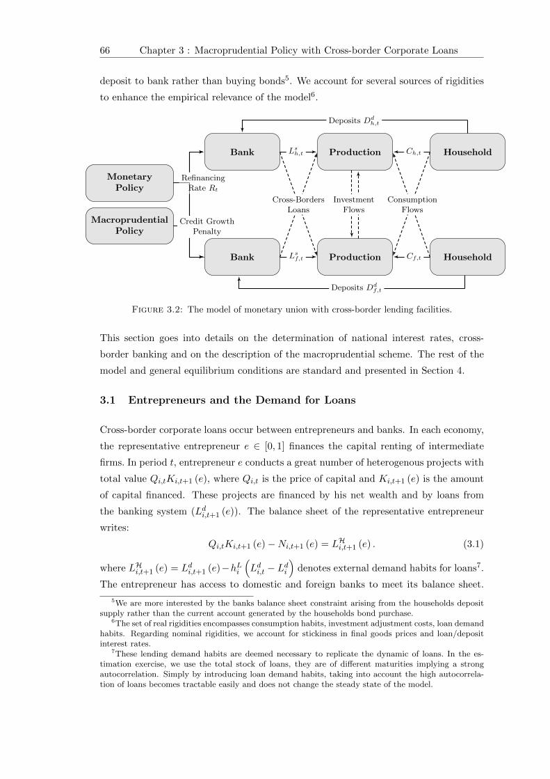
66 Chapter 3 : Macroprudential Policy with Cross-border Corporate Loans
deposit to bank rather than buying bonds5. We account for several sources of rigidities
to enhance the empirical relevance of the model6.
MonetaryPolicy
MacroprudentialPolicy
Bank
Bank
Production
Production
Household
Household
Ch,t
Cf,t
Lsh,t
Lsf,t
InvestmentFlows
ConsumptionFlows
Cross-BordersLoans
RefinancingRate Rt
Credit GrowthPenalty
Deposits Ddh,t
Deposits Ddf,t
Figure 3.2: The model of monetary union with cross-border lending facilities.
This section goes into details on the determination of national interest rates, cross-
border banking and on the description of the macroprudential scheme. The rest of the
model and general equilibrium conditions are standard and presented in Section 4.
3.1 Entrepreneurs and the Demand for Loans
Cross-border corporate loans occur between entrepreneurs and banks. In each economy,
the representative entrepreneur e ∈ [0, 1] finances the capital renting of intermediate
firms. In period t, entrepreneur e conducts a great number of heterogenous projects with
total value Qi,tKi,t+1 (e), where Qi,t is the price of capital and Ki,t+1 (e) is the amount
of capital financed. These projects are financed by his net wealth and by loans from
the banking system (Ldi,t+1 (e)). The balance sheet of the representative entrepreneur
writes:
Qi,tKi,t+1 (e)−Ni,t+1 (e) = LHi,t+1 (e) . (3.1)
where LHi,t+1 (e) = Ldi,t+1 (e)−hLi(Ldi,t − Ldi
)denotes external demand habits for loans7.
The entrepreneur has access to domestic and foreign banks to meet its balance sheet.
5We are more interested by the banks balance sheet constraint arising from the households depositsupply rather than the current account generated by the households bond purchase.
6The set of real rigidities encompasses consumption habits, investment adjustment costs, loan demandhabits. Regarding nominal rigidities, we account for stickiness in final goods prices and loan/depositinterest rates.
7These lending demand habits are deemed necessary to replicate the dynamic of loans. In the es-timation exercise, we use the total stock of loans, they are of different maturities implying a strongautocorrelation. Simply by introducing loan demand habits, taking into account the high autocorrela-tion of loans becomes tractable easily and does not change the steady state of the model.

Chapter 3 : Macroprudential Policy with Cross-border Corporate Loans 67
The total amount borrowed by the representative entrepreneur writes:
Ldi,t+1 (e) =((
1− αLi)1/ν
Ldh,i,t+1 (e)(ν−1)/ν +(αLi)1/ν
Ldf,i,t+1 (e)(ν−1)/ν)ν/(ν−1)
, (3.2)
where parameter ν is the elasticity of substitution between domestic and foreign loans,
αLi represents the percentage of cross-border loan flows in the monetary union and
Ldh,i,t+1 (e) (resp. Ldf,i,t+1 (e)) the amount of domestic (resp. foreign) loans demanded
by entrepreneur e in country i. The total cost of loans, pLi,t, is thus defined according to:
pLi,t (e) =((
1− αLi)rLh,t (e)1−ν + αLi r
Lf,t (e)1−ν
)1/(1−ν), (3.3)
where rLh,t (e) (resp. rLf,t (e)) is the cost of loans obtained from home (resp. foreign)
banks by entrepreneur e in country i. The decision to borrow from a particular bank is
undertaken on the basis of relative national interest rates:
Ldh,i,t+1 (e) =(1− αLi
)[rLh,t (e)
pLi,t (e)
]−νLdi,t+1 (e) , and, Ldf,i,t+1 (e) = αLi
[rLf,t (e)
pLi,t (e)
]−νLdi,t+1 (e) .
The investment projects undertaken by the entrepreneur are risky and differ with respect
to their individual returns. To model individual riskiness, we assume that each project
has an individual return equal to ωRki,t, i.e. that the aggregate return of investment
projects in the economy Rki,t is multiplied by a random value ω (drawn from a Pareto
distribution8). Defining the value for a profitable project by ωi,t(e) = E(ω|ω ≥ ωCi,t(e)
)
(where ωCi,t (e) is the critical value of ω that distinguishes profitable and non profitable
projects), the profit function of entrepreneur e after aggregating all projects writes:
ΠEi,t+1 (e) =
ωi,t+1
(1 + rki,t+1
)Qi,tKi,t+1 (e)−
(1 + pLi,t (e)
)LHi,t+1 (e) with probability ηEi,t+1,
0 with probability 1− ηEi,t+1,.
(3.4)
where ηEi,t+1 is the time-varying expected share of gainful projects. Since entrepreneurs
cannot screen the value of ωi,t+1 (e) ex ante, ωCi,t(e) cannot be a control variable of the
financial contract between borrowers and lenders contrary to Bernanke et al. (1999). To
introduce a financial accelerator mechanism, we borrow a concept of De Grauwe (2010)
applied in a different context, by assuming that entrepreneurs’ forecasts regarding the
8With respect to the standard framework standardly used in the literature (Bernanke et al., 1999),we assume that the heterogeneity in the return of investment project undertaken by firms is modeledusing a Pareto distribution. This device commonly used in other branches of the economic literatureprovides a series of interesting features in the analysis and allows an easier estimation of the financialamplification effect. See in appendices subsubsection 1.5.2 (page 185) for details about the computationof ω.

68 Chapter 3 : Macroprudential Policy with Cross-border Corporate Loans
aggregate profitability of a given project ωi,t(e) are optimistic (i.e., biased upwards)9.
The perceived ex ante value of profitable projects is defined by the isoleastic function:
g(ωi,t+1, ε
Qi,t
)= γi (ωi,t+1)
κi(κi−1)
(eεQi,t
) 1
(κi−1) ,
where εQi,t is an AR(1) process10, κi is the elasticity of the external finance premium11
and γi is a scale parameter12. In this expression, the exogenous shock is affected by
exponent 1/ (κi − 1) to normalize to unity the impact of the financial shock εQi,t in the
log deviation form of the model. Thus, ex-ante the entrepreneur chooses a capital value
of Ki,t+1 (e) that maximizes its expected profit defined as:
max{Ki,t+1(e)}
Et{ηEi,t+1
[g(ωi,t+1, ε
Qi,t
)(1 + rki,t+1
)Qi,tKi,t+1 (e)−
(1 + pLi,t (e)
)LHi,t+1 (e)
]}.
(3.5)
Using the characteristics of the Pareto distribution, the expected spread required by
representative entrepreneur e to undertake the decision to finance firms’ investment is:
Si,t (e) =Et(
1 + rki,t+1
)
1 + pLi,t (e)= γκi−1
i
[κ
κ− 1
(1− Ni,t+1 (e)
Qi,tKi,t+1 (e)
)]κieεQi,t . (3.6)
The size of the accelerator is determined by the elasticity of the external finance premium
κi. For κi > 0, the external finance premium is a positive function of the leverage
ratio, Qi,tKi,t+1 (e) /Ni,t+1 (e), so that an increase in net wealth induces a reduction
of the external finance premium. This phenomenon disappears if κi = 0. Concerning
the exogenous movements of the external finance premium, a positive realization of εQi,t
means that entrepreneurs require a higher expected profitability of capital Etrki,t+1 to
finance investment for a given level of lending conditions pLi,t. Furthermore, a shock that
hits the entrepreneur net wealth Ni,t+1 (e) will also affect the rentability of the physical
capital in the economy. As the rentability of capital is a cost for the intermediate sector,
a variation in the net wealth will have aggregate consequences on goods supply through
the channel of the capital market as underlined by Gilchrist, Sim, & Zakrajsek (2009).
The amount of capital of non-profitable entrepreneurs’ investment projects is consumed
9Assuming optimistic firms is motivated empirally, Bachmann & Elstner (2013) find evidence of suchexpectations for German firms using microdata. This hypothesis of the expectations of the private sectoris very close to the utility functions introduced by Goodhart et al. (2005) for bankers. In our setting,the financial accelerator does not result from a moral hazard problem but rather from a bias in theexpectations of the private sector.
10This shock affects the expected profitability of financial projects by rising in exogeneously the riskpremium implying an increase in the cost of capital and hence a reduction in investment as underlinedby Gilchrist, Sim, & Zakrajsek (2009) for the US economy.
11The elasticity of the external finance premium expresses the degree of bias in estimating the expectedrentability of entrepreneurs’ projects such that if ω > 1 and κi > 0 then g (ω) > ω. Expressed a
la De Grauwe (2010), Eoptt ωi,t+1 = Etγi (ωi,t+1)κi/(κi−1) where Eoptt is the expectation operator ofoptimistic entrepreneurs.
12This parameter is needed to make the steady state independent of κi ,such that γi = ω1/(1−κi).

Chapter 3 : Macroprudential Policy with Cross-border Corporate Loans 69
in terms of home final goods Pi,t
(1− ηEi,t
)ωi,t (e)
(1 + rki,t
)Qi,t−1Ki,t (e). Thus the net
wealth of the entrepreneur in the next period is equal to:
Ni,t+1 (e) =(1− τEi
) ΠEi,t (e)
eεNi,t
, (3.7)
where εNi,t is an exogenous process of net wealth destruction and τEi is a proportional
tax on the profits of the bank.
3.2 The Banking Sector and the Imperfect Pass-Through of Policy
Rate
The representative bank b in country i collects deposits from households and lends to
firms. The balance sheet of the bank writes:
Lsi,t+1 (b) = Di,t+1 (b) + LRFi,t+1 (b) +BKi,t+1 (b) . (3.8)
In this expression, Lsi,t is the total level of loans supplied by bank b, Di,t (b) is the total
level of deposit services offered by bank b of country i to households, LRFi,t+1 (b) is the
one-period refinancing loans to banks by the ECB and BKi,t+1 (b) is the bank capital.
The representative bank sets the rate of interest rLi,t (b) and rDi,t (b).
Banks finance heterogenous investment projects conducted by home and foreign en-
trepreneurs, some of these projects are gainful with a probability ηi,t+1. Following
Bernanke et al. (1999), if the borrower’s project is gainful, the representative bank ob-
tains ηi,t+1(1 + rLi,t (b))Lsi,t+1 (b), whereas if the entrepreneur’s project is insolvent, the
bank must pay auditing costs µB to obtain its loan13, thereby the expected value of next
period earnings is:
EtΠBi,t+1 (b) =
[Etηi,t+1 +
(1− µB
)(1− ηi,t+1)
] (1 + rLi,t (b)
)Lsi,t+1 (b)
︸ ︷︷ ︸Revenues from loan supply activities
(3.9)
− (1 + rt)LRFi,t+1 (b)
︸ ︷︷ ︸ECB refinancing cost
−(1 + rDi,t
)Di,t+1 (b)
︸ ︷︷ ︸Deposit cost
.
In this setting, we assume that there is no discrimination between borrowers, so that
the representative and risk-neutral bank serves both domestic and foreign entrepreneur
without taking into account specificities regarding the national viability of projects. Since
banks lend to both home and foreign entrepreneurs, the expected share of profitable
13i.e., banks recover(1− µB
)(1− ηi,t+1) (1 +RLi,t (b))Lsi,t+1 (b): we borrow this shortcut from Benes
et al. (2014) which is a tractable and easier way to introdue the loss given to default µB than in theinial framework of Bernanke et al. (1999) where investors have a technology to size the collateral in caseof default.

70 Chapter 3 : Macroprudential Policy with Cross-border Corporate Loans
projects is determined by a geometric average, ηi,t =(ηEh,t
)(1−αLh) (ηEf,t
)αLfη(αLh−αLf )
where η is the steady state share of profitable investment projects14. Concerning bank
capital, we follow Hirakata et al. (2009) by assuming the law of motion of the net wealth
is made of the profits of the previous period:
BKi,t+1 (b) =(1− τBi
)ΠBi,t (b) , (3.10)
where τBi denotes a proportional tax on the revenues of the bank by national govern-
ments15.
As in Darracq-Paries et al. (2011), we take into account the imperfect pass-through of
policy rate on bank lending/deposit rates. We suppose that banks set their interest
rates on a staggered basis with some degree of nominal rigidity a la Calvo.
3.2.1 Loan supply decisions
The determination of interest rate on loans is as follows: the representative bank b
maximizes expected profit from Equation 3.9 with respect to Lsi,t+1 (b) to obtain the
expression of the marginal cost of producing new loans:
1 +MCLi,t (b) =(1 + rt)
[1− µB (1− Etηi,t+1)]. (3.11)
The representative retail bank b acts monopolistically to provide loans to entrepreneurs.
It determines the interest rate on loans contracted by entrepreneurs. Assuming that it
is able to modify its loan interest rate with a probability 1 − θLi , it chooses rL∗i,t (b) to
maximize its expected sum of profits:
max{RL∗i,t (b)}
Et
{ ∞∑
τ=0
(θLi β
)τ λci,t+τλci,t
[rL∗i,t (b)−MCLi,t+τ
]Li,t+1+τ (b)
},
subject to the demand constraint, Li,t+1+τ (b) = 1ni
(rL∗i,t (b) /rLi,t+τ
)−εLLi,t+1+τ , τ > 0,
where Li,t (b) denotes the quantity of differentiated banking loans b that is used in loans
packer production. Finally, the interest rate that solves the FOC for the bank that is
allowed to modify its interest rate, it is such that:
Et∞∑
τ=0
(θLi β
)τ λci,t+τλci,t
[rL∗i,t (b)− εL
(εL − 1)MCLi,t+τ
]Li,t+1+τ (b) = 0. (3.12)
14In steady state, we suppose that banks are symmetric between countries such that when η = ηEh = ηEfand εb = εbh = εbf , then RL = RLh = RLf .
15This tax is necessary to solve up the model in steady state. Bernanke et al. (1999) and Hirakata etal. (2011) also add a proportional cost in law of motion of the net wealth.

Chapter 3 : Macroprudential Policy with Cross-border Corporate Loans 71
3.2.2 Deposit supply decisions
We proceed accordingly for the determination of deposit interest rate. The nominal
marginal cost of one unit of deposit denoted by MCDi,t is the same across banks and is
related to the ECB refinancing rate:
1 +MCDi,t (b) = 1 +MCDi,t = (1 + rt) . (3.13)
Assuming sticky deposit rates, the expected sum of profits for the bank that is allowed
to modify its interest rate with a probability 1− θDi writes:
max{RD∗i,t (b)}
Et
{∑∞τ=0
(θDi β
)τ λci,t+τλci,t
[MCDi,t+τ − rD∗i,t (b)
]Di,t+1+τ (b)
}, (3.14)
under the constraint, Di,t+1+τ (b) = 1ni
(rD∗i,t (b) /rDi,t+τ
)−µDi,t+τ/(µDi,t+τ−1)Ddi,t+1+τ , ∀τ >
0, where µDi,t = εD/(εD − 1
)+ εDi,t is the time-varying markup subject to the exogenous
deposit rate-push shock process εDi,t. The interest rate that solves the FOC for the bank
that is allowed to modify its interest rate writes:
∑∞τ=0
(θDi β
)τ λci,t+τλci,t
1
µDi,t+τ − 1
[rD∗i,t (b)− µDi,t+τMCDi,t+τ
]Di,t+1+τ (b) = 0. (3.15)
3.3 Macroprudential Policy
As in Fatas & et al. (2009), Quint & Rabanal (2013) and Bailliu et al. (2012) we introduce
a macroprudential tool based on credit growth to affect the general equilibrium of the
economy through the lending conditions of commercial banks. We more particularly
evaluate how the choice of a particular institutional setting based on the global or
regional financial developments of the Eurozone may affect economic outcomes. As
shown in Table 3.1, our analysis contrasts seven situations, combining the definition
of the global or regional value of the macroprudential instrument and the uniform or
heterogenous setting of the macroprudential parameter between member countries.
Global solutions: under this macroprudential scheme, authorities react to the average
per capita credit growth in the Monetary Union16. We contrast three possibilities: in the
first situation, the macroprudential concern of the authorities gives rise to an extended
interest rate of the central bank. The monetary policy rule is augmented to allow the
16Namely we set MPu,t =(Lsc,t/L
sc,t−1
)n (Lsp,t/L
sp,t−1
)1−n.

72 Chapter 3 : Macroprudential Policy with Cross-border Corporate Loans
policy interest rate to react to the average credit growth in Equation 3.22:
1 + rt = f (πu,t, Yu,t)× (MPu,t)φ ,
where MPu,t is the macroprudential instrument and φ is the macroprudential policy
stance on the central bank interest rate. Under this first scheme, lending and deposit
conditions are affected by macroprudential policy through the cost of bank refinancing
by the central bank open market decisions. This situation will be treated below as a
variant of the optimal monetary policy rule set by the central bank.
In the second and third situations macroprudential measures are implemented at the
commercial bank level, through the marginal cost of loan production and are totally
separated from monetary policy decisions. A tightening of credit conditions due to
macroprudential measures increases the interest rate faced by borrowers by modifying
the marginal cost of credit (see Equation 3.11) in the economy17:
1 +MCLi,t =(1 + rt) (MP i,t)φi
1− µB (1− Etηi,t+1). (3.16)
We consider that macroprudential authorities are concerned by credit growth and lean
against the build-up of emerging financial imbalances. In the second situation, macro-
prudential authorities penalize the average growth of credit by affecting proportionally
the lending rate of bank in Equation 3.16 with a common degree of penalization φh = φf
taking into account average developments in the Eurozone systemic risk. In the third
situation, macroprudential authorities penalize the average growth of credit by affecting
proportionally the lending rate of bank in Equation 3.16 with a degree of penalization
set at the regional level (φh 6= φf ).
National solutions: under this macroprudential scheme, measures take into account
the regional evolution of loans (i.e., MPh,t 6= MPf,t) but apply a similar uniform
parameter to all the participating countries (i.e., φc = φp = φ). However, as cross
border lending leads to alternative way of implementing macroprudential measures at the
national level (focussing on lenders or borrowers) we take into account two possibilities.
In the first situation, macroprudential authorities focus on the evolution of loan supply
in their economy (i.e., react to the lending decision of their national banking sector) so
that, MP i,t =(Lsi,t/L
si,t−1
)for i ∈ {c, p}. This solution provides a common reaction
of national financial developments in each part of the monetary union. In the second
situation, macroprudential authorities focus on the evolution of loan demand in their
economy (i.e., react to the borrowing decision of national entrepreneur) so that,MP i,t =
17Under staggered interest rates, the diffusion of the macroprudential policy does not work perfectlyas there is imperfect pass-through.

Chapter 3 : Macroprudential Policy with Cross-border Corporate Loans 73
Scenario InstrumentPolicyStance
PolicyChannel
Extended rule MPu,t =(Lsc,t/L
sc,t−1
)n (Lsp,t/L
sp,t−1
)1−nφc = φp = φ 1 + rt = f (πu,t, Yu,t)× (MPu,t)φ
Global 1 MPu,t =(Lsc,t/L
sc,t−1
)n (Lsp,t/L
sp,t−1
)1−nφc = φp = φ 1 +MCLi,t =
(1+rt)(MPu,t)φ
[1−µB(1−Etηi,t+1)]
Global 2 MPu,t =(Lsc,t/L
sc,t−1
)n (Lsp,t/L
sp,t−1
)1−nφc 6= φp 1 +MCLi,t =
(1+rt)(MPu,t)φi
[1−µB(1−Etηi,t+1)]
National 1 MPi,t =(Lsi,t/L
si,t−1
)for i ∈ {c, p} φc = φp = φ 1 +MCLi,t =
(1+rt)(MPi,t)φ
[1−µB(1−Etηi,t+1)]
National 2 MPi,t =(Ldi,t/L
di,t−1
)for i ∈ {c, p} φc = φp = φ 1 +MCLi,t =
(1+rt)(MPi,t)φ
[1−µB(1−Etηi,t+1)]
Granular 1 MPi,t =(Lsi,t/L
si,t−1
)for i ∈ {c, p} φc 6= φp 1 +MCLi,t =
(1+rt)(MPi,t)φi
[1−µB(1−Etηi,t+1)]
Granular 2 MPi,t =(Ldi,t/L
di,t−1
)for i ∈ {c, p} φc 6= φp 1 +MCLi,t =
(1+rt)(MPi,t)φi
[1−µB(1−Etηi,t+1)]
Table 3.1: Different levels of implementation of Macroprudential policy
(Ldi,t/L
di,t−1
)for i ∈ {c, p}. This solution is interesting as it takes into account foreign
loan supply directed towards the domestic economy (and vice-versa).
Granular solutions: granular solution combines a national appreciation of the evo-
lution of loans and a national setting of the macroprudential parameter. In the first
situation, authorities focus on lenders (i.e., on the banking system) and by so directly
affect the main origin of the distribution of loans in the economy (captured by the home
bias in loan demand). Here, MP i,t =(Lsi,t/L
si,t−1
)for i ∈ {c, p} with φc 6= φp. In this
situation, authorities are not able to address the exact quantity of loans contracted in
the economy (the quantify of loans distributed by foreign banks in the economy is not
accounted for in Lsi,t while the quantity of national loans sold to foreign entrepreneurs
is part of Lsi,t). This in turn, implies a wrong evaluation of the evolution of systemic
risk in the economy and generates externalities between member countries of the mon-
etary union (as the national macroprudential stance affects the other economy through
the lending conditions to foreign agents). In the second situation authorities focus on
borrowers (Here, MP i,t =(Ldi,t/L
di,t−1
)for i ∈ {c, p} with φc 6= φp. ). Authorities have
a better understanding of the amount of loans contracted by national agents (i.e., this
system eliminates the shadow nature of the foreign banks that operate domestically).
However in this situation they are unable to affect directly the origin of loan distribution.
4 The rest of the model
Due to the asymmetry between countries, for each variable denotedXi,t (x), we aggregate
households, firms, entrepreneurs and banks using the following aggregator for agent

74 Chapter 3 : Macroprudential Policy with Cross-border Corporate Loans
x ∈ [0, np + nc] living in the monetary union:
G (Xi,t (x)) =
{ ∫ n0 Xc,t (x) dx for i = c∫ 1nXp,t (x) dx for i = p
. (3.17)
4.1 Households
In each economy there is a continuum of identical households who consume, save and
work in intermediate firms. The total number of households is normalized to 1. The
representative household j ∈ [0, 1] maximizes the welfare index:
max{Ci,t(j),Hi,t(j),Ddi,t+1(j)}
Et∞∑
τ=0
βτeεUi,t+τ
(Ci,t+τ (j)− hCi Ci,t−1+τ
)1−σCi1− σCi
− χiH
1+σLi
i,t+τ (j)
1 + σLi
,
(3.18)
subject to:
Wi,t
PCi,tHi,t (j)+
(1 + rDi,t−1
) Ddi,t (j)
PCi,t+
ΠYi,t (j)
PCi,t+Mi (j)
PCi,t= Ci,t (j)+
Ddi,t+1 (j)
PCi,t+Ti,t (j)
PCi,t+Pi,t
PCi,tACDi,t (j)
Here, Ci,t (j) is the consumption index, hCi ∈ [0, 1] is a parameter that accounts for
external consumption habits, Hi,t (j) is labor effort, εUi,t is an exogenous AR(1) shock
to household preferences. The income of the representative household is made of labor
income (with nominal wage, Wi,t ), interest payments for deposits, (where Ddi,t (j) stands
for the deposit subscribed in period t − 1 and 1 + rDi,t−1 is the gross nominal rate of
interest between period t−1 an period t), and earnings ΠYi,t (j) from shareholdings. The
representative household spends this income on consumption, deposits and tax payments
(for a nominal amount of Ti,t (j)). Finally, he has to pay quadratic adjustment costs
to buy new deposit services (Schmitt-Grohe & Uribe, 2003), according to the function,
ACDi,t (j) =χDi2
(Ddi,t+1(j)−Ddi (j))2
Ddi (j), where Dd
i (j) is the steady state level of deposits. In
order to make the households/banks deposit problem tractable in the steady state18, we
assume that households hold a constant quantity of real money balances Mi (j).
The first order conditions that solve this problem can be summarized with an Euler
condition:
β(
1 + rDi,t
)
1 + Pi,tACD′i,t (j)= Et
{eεUi,t
eεUi,t+1
PCi,t+1
PCi,t
(Ci,t+1 (j)− hCi Ci,tCi,t (j)− hCi Ci,t−1
)σCi }, (3.19)
18The lending supply is asymmetric between the two areas wich implies asymmetric refinancing oper-ations and deposits. In order to have symmetric households in steady state between core and periphery,we suppose that households hold a constant quantity of real money balances.

Chapter 3 : Macroprudential Policy with Cross-border Corporate Loans 75
and a labor supply function:
Wi,t
PCi,t= χiHi,t (j)σ
Li(Ci,t (j)− hCi Ci,t−1
)σCi . (3.20)
The consumption basket of the representative household and the consumption price in-
dex of country i are, Ci,t(j) = ((1− αCi
)1/µCh,i,t(j)
(µ−1)/µ+(αCi)1/µ
Cf,i,t (j)(µ−1)/µ
)µ/(µ−1)
and PCi,t = ((1− αCi
)P 1−µh,t + αCi P
1−µf,t )1/(1−µ) where µ is the elasticity of substitution
between the consumption of home (Ch,i,t(j)) and foreign (Cf,i,t (j)) goods and αCi is the
degree of openness of the economy i. In this model, we assume home bias in consump-
tion, so that αCi <12 .
4.2 Firms
This sector is populated by two groups of agents: intermediate firms and final firms.
Intermediate firms produce differentiated goods i, choose labor and capital inputs, and
set prices according to the Calvo model. Final goods producers act as a consumption
bundler by combining national intermediate goods to produce the homogenous final
good19.
Concerning the representative intermediate firm i, it has the following technology, Yi,t (i) =
eεAi,tKi,t (i)αHd
i,t (i)1−α, where Yi,t (i) is the production function of the intermediate good
that combines capital Ki,t (i), labor Hdi,t (i) and technology eε
Ai,t (an AR(1) productivity
shock). Intermediate goods producers solve a two-stages problem. In the first stage,
given the input prices Wi,t and Zi,t as given, firms rent inputs Hdi,t (i) and Ki,t (i) in a
perfectly competitive factor markets in order to minimize costs subject to the production
constraint. The first order condition leads to the marginal cost expression:
MCi,t(i) = MCi,t =1
eεAi,t
(Zi,tα
)α( Wi,t
(1− α)
)(1−α)
. (3.21)
From the cost minimization problem, inputs also satisfy, αHdi,t (i)Wi,t = Zi,tKi,t (i) (1− α).
In the second-stage, firm i sets the price according to a Calvo mechanism. Each period
firm i is not allowed to reoptimize its price with probability θPi but price increases
of ξPi ∈ [0; 1] at last period’s rate of price inflation, Pi,t (i) = πξPii,t−1Pi,t−1 (i). The firm
allowed to modify its selling price with a probability 1−θPi chooses{P ∗i,t(i)
}to maximize
19Final good producers are perfectly competitive and maximize profits, Pi,tYdi,t− G (Pi,t (i)Yi,t (i)),
subject to the production function Y di,t = ((1/ni)1/εP G
(Yi,t (i)(εP−1)/εP
))εP /(εP−1). We find the inter-
mediate demand functions associated with this problem are, Yi,t (i) = (1/ni) (Pi,t(i)/Pi,t)−εP Y di,t, ∀i.
where Y di,t is the aggregate demand.

76 Chapter 3 : Macroprudential Policy with Cross-border Corporate Loans
its expected sum of profits:
max{P ∗i,t(i)}
Et
{∑∞τ=0
(θPi β
)τ λci,t+τλci,t
[P ∗i,t (i)
PCi,t+τ
τ∏k=1
πξPii,t+k−1 −
MCi,t+τ
PCi,t+τ
]Yi,t+τ (i)
},
under the demand constraint:
Yi,t+τ (i) =1
ni
(∏τk=1π
ξPii,t+k−1
P ∗i,t (i)
Pi,t+τ
)−εPY di,t+τ , ∀ τ > 0,
where Y di,t represents the quantity of the goods produced in country i and λci,t the house-
hold marginal utility of consumption.
4.3 Monetary Policy
The central bank of the monetary union follows an interest rate rule defined by:
(1 + rt1 + r
)=
(1 + rt−1
1 + r
)ρ((πCu,t)φπ
(Yu,tYu,t−1
)φ∆y)(1−ρ)
eεRt , (3.22)
where rt is the interest rate set by the central bank, ρ is the interest rate smoothing
coefficient, εRt is an exogenous AR(1) monetary policy shock common to the monetary
union members, φπ is the level of reaction to inflation, φ∆y is the GDP growth target.
In this expression, union-wide inflation and GDP growth are defined by a geometric
average that account for the relative size of each country, πCu,t =(πCc,t)n (
πCp,t)1−n
and
Yu,t = (Yc,t)n (Yp,t)
1−n.
4.4 Capital Suppliers
Capital suppliers are homogeneous and distributed over a continuum normalized to one.
The representative capital supplier k acts competitively to supply a quantity Ki,t+1 (k) of
capital. Investment is costly, i.e. the capital supplier pays an adjustment cost ACIi,t (k)
on investment, such that ACIi,t (k) =χIi2
(eεIi,tIi,t (k) /Ii,t−1 (k)− 1
)2where εIi,t is an
exogenous adjustment cost shock on investment. The capital stock of the representative
capital supplier thus evolves according to:
Ki,t+1 (k) =(1−ACIi,t (k)
)Ii,t (k) + (1− δ)Ki,t (k) .
The capital supplier produces the new capital stock Qi,tKi,t+1 (k) by buying the depre-
ciated capital Qi,t (1− δ)Ki,t (k) and investment goods P Ii,tIi,t (k) where:
Ii,t (k) =((
1− αIi)1/µ
Ihi,t (k)(µ−1)/µ +(αIi)1/µ
Ifi,t (k)(µ−1)/µ)µ/(µ−1)
,

Chapter 3 : Macroprudential Policy with Cross-border Corporate Loans 77
and:
P Ii,t =((
1− αIi)
(Ph,t)1−µ + αIi (Pf,t)
1−µ)1/(1−µ)
.
In this expression, parameter µ is the elasticity of substitution between domestic and
foreign goods in investment and αIi < 0.5 measures the degree of investment diversifi-
cation in the monetary union between home and foreign countries. The representative
capital supplier chooses Ii,t (k) to maximize profits:
max{Ii,t(k)}
Et
{∑∞τ=0
βτλci,t+τλci,t
[Qi,t
(1−ACIi,t (k)
)− P Ii,t
]Ii,t (k)
},
where βτλci,t+τλci,t
is the household stochastic discount factor. The price of capital renting
thus solves:
Qi,t = P Ii,t +Qi,t∂(Ii,t (k)ACIi,t (k)
)
∂Ii,t (k)+ βEt
λci,t+1
λci,tQi,t+1
∂(Ii,t+1 (k)ACIi,t+1 (k)
)
∂Ii,t (k).
Thus, the real return from holding one unit of capital from t to t+ 1 is determined by:
Et
(1 + rki,t+1
)
πCi,t+1
= Et
[Zi,t+1/P
Ci,t+1 + (1− δ)Qi,t+1/P
Ci,t+1
Qi,t/PCi,t
]. (3.23)
4.5 Governments
National governments finance public spending by charging proportional taxes on the
bank capital τBi , net wealth of entrepreneurs τEi and by receiving a total value of taxes
G (Ti,t (j)) from households. The budget constraint of the national government writes:
G (Ti,t (j)) + τEi G (Ni,t (e)) + τBi G (BKi,t (b)) = Pi,tGi,t = Pi,tGεGi,t,
where Gi,t is the total amount of public spending in the ith economy that follows
an AR(1) shock process. Following Smets & Wouters (2007), we assume that exoge-
nous spending is affected by the productivity shock at a degree ρagi such that εGi,t =
ρGi εGi,t−1 + ηGi,t + ρagi η
Ai,t. The government demand for home goods writes, Gi,t (i) =
(Pi,t (i) /Pi,t)−εP Gi,t.
4.6 Aggregation and Market Equilibrium
In this model, there are 8 country specific structural shocks for i ∈ {c, p} and one
common shock in the Taylor rule. For s = {U,A, I,Q,N,D}, the shocks follow a

78 Chapter 3 : Macroprudential Policy with Cross-border Corporate Loans
first order autoregressive process such that εsi,t = ρsi εsi,t−1 + ηsi,t while for exogenous
spending the process reads as follows: εGi,t = ρGi εGi,t−1 + ηGi,t + ρagηAi,t. In these first-order
autoregressive process, ρUi , ρAi , ρGi , ρIi , ρQi , ρNi , ρDi and ρR are autoregressive roots
of the exogenous variables. ηUi,t, ηAi,t, η
Gi,t, η
Ii,t, η
Qi,t, η
Ni,t, η
Di,t and ηRt are standard errors
that are mutually independent, serially uncorrelated and normally distributed with zero
mean and variances σ2i,U , σ2
i,A, σ2i,G, σ2
i,I , σ2i,Q, σ2
i,N , σ2i,D and σ2
R respectively. A general
equilibrium is defined as a sequence of quantities {Qt}∞t=0 and prices {Pt}∞t=0 such that
for a given sequence of quantities {Qt}∞t=0 and the realization of shocks {St}∞t=0, the
sequence {Pt}∞t=0 guarantees the equilibrium on the capital, labor, loan, intermediate
goods and final goods markets.
After (i) aggregating all agents and varieties in the economy, (ii) imposing market
clearing for all markets, (iii) substituting the relevant demand functions, we deduct the
general equilibrium conditions of goods, loans and deposit services markets.
4.6.1 Goods Market
The aggregate price index of the national goods evolves according to:
P 1−εPi,t = θPi
[Pi,t−1
(Pi,t−1
Pi,t−2
)ξPi]1−εP
+(1− θPi
) (P ∗i,t)1−εP . (3.24)
The equilibrium condition on the final goods market writes is defined by the aggregation
of the demand function from final goods producers, G (Yi,t (i)) = Y di,tG (Pi,t(i)/Pi,t)
−εP
where G (Yi,t (i)) = eεAi,tG
(Ki,t (i)αHd
i,t (i)1−α)
is the aggregation of intermediate goods
suppliers and Y di,t is the resources constraint. Thus, replacing the demand functions of
foreign and home goods (consumption and investment), we finally obtain the home final
goods market equilibrium in the home country:
Yc,t
∆Pc,t
=(1− αCc
)(Pc,t
PCc,t
)−µCc,t +
(1− αIc
)(Pc,t
P Ic,t
)−µ (1 +ACIc,t
)Ic,t (3.25)
+n− 1
n
(αCp
(Pc,t
PCp,t
)−µCp,t + αIp
(Pc,t
P Ip,t
)−µ (1 +ACIp,t
)Ip,t
)
+Gc,t +ACDc,t,
where ∆Pi,t = G (Pi,t (i) /Pi,t)
−εP denotes the price dispersion term, which is induced by
the assumed nature of price stickiness, is inefficient and entails output loss. To close
the model, adjustment costs on deposits are entirely home biased:
ACDi,t = G(ACDi,t (i)(εP−1)εP )
εP(εP−1) ,

Chapter 3 : Macroprudential Policy with Cross-border Corporate Loans 79
the associated demand function writes, ACDi,t (i) = (Pi,t (i) /Pi,t)−εP ACDi,t.
4.6.2 Loan Market
Concerning the equilibrium on loan market, it is defined by the aggregate demand func-
tion from retail banks, G(Lsi,t+1 (b)
)= ∆L
i,tLdi,t+1, where ∆L
i,t = G(rLi,t (b) /rLi,t
)−εLis
the credit rate dispersion term and Ldi,t+1 is the aggregate demand from home and for-
eign entrepreneurs, and is defined by, Ldi,t+1 = G (Lh,i,t+1 (e))+G (Lf,i,t+1 (e)). Recalling
that entrepreneurs e borrow to domestic and foreign banks with varieties b produced by
wholesale branches, the equilibrium finally writes in the home country:
Lsc,t+1 =
((1− αLc
)[rLc,t
pLc,t
]−νLc,t+1 +
n
n− 1αLf
[rLc,t
pLp,t
]−νLp,t+1
)∆Lc,t. (3.26)
Aggregate loan rate index evolves according to:
(rLi,t)1−εL
= θLi(rLi,t−1
)1−εL+(1− θLi
) (rLi,t)1−εL
. (3.27)
4.6.3 Deposit Market
Eventually the equilibrium on deposit market is defined by the aggregate demand for
deposits services of households and the aggregate supply from deposit packers. Ag-
gregating the demand function from deposit packers leads to the equilibrium on this
market, G (Di,t+1 (b)) = ∆Di,tG
(Ddi,t+1 (j)
), where ∆D
i,t = G(rDi,t (b) /rDi,t)−µDi,t/(µDi,t−1) is
the interest rate dispersion term, while the aggregate deposit rate index evolves accord-
ing to:(rDi,t) 1
1−µDi,t = θDi
(rDi,t−1
) 1
1−µDi,t +
(1− θDi
) (rDi,t) 1
1−µDi,t . (3.28)
5 Estimation
5.1 Data
We split the Eurozone in two groups: core and periphery. Since EMU creation, coun-
tries with current account surpluses belong to the core country group, other countries
belong to the peripheral group20. France is halfway since its current account had been
20Core countries: Austria, Belgium, Germany, Finland, France, Luxembourg and the Netherlands.Peripheral countries: Spain, Greece, Ireland, Italy and Portugal.

80 Chapter 3 : Macroprudential Policy with Cross-border Corporate Loans
positive from 1999 to 2003, we make the hypothesis that France is still a core coun-
try despite its recent current account deficits21. The model is estimated with Bayesian
methods on Eurozone quarterly data over the sample period 1999Q1 to 2013Q3, which
makes 59 quarterly observations for each variable (except for financial variables). The
dataset includes 15 times series: real GDP (Eurostats), real consumption (Eurostats),
real investment (Eurostats), the ECB refinancing operation rate (Eurostats, one year
maturity), the HICP (ECB, overall index, deseasonalized using a multiplicative decom-
position), the overnight deposit rate of households and firms (ECB), the outstanding
amount of loan and lending rate to non-financial corporations (ECB, 2003-2013, desea-
sonalized using a multiplicative decomposition). Data with a trend are made stationary
using a linear trend and are divided by the population. We also demean the data be-
cause we do not use the information contained in the observable mean. Figure 3.3 plots
the transformed data.
2000 2006 2011
−2
0
2∆ log Production
2000 2006 2011
−2
0
2
∆ log Consumption
2000 2006 2011
−5
0
5
∆ log Investment
2000 2006 2011−0.5
00.5
11.5
∆ log HICP
2000 2006 2011−4−2
024
∆ log Loan Supply
2000 2006 20112
4
6
Loan Interest Rate
Core countries Peripheral countries Euro Area
2000 2006 2011
0.5
1
1.5Deposit Rate
2000 2006 2011
2
4
ECB Interest Rate
Figure 3.3: Observable variables
5.2 Calibration and Priors
The complete set of calibrated parameters is reported in Table 3.2. We fix a small
number of parameters commonly used in the literature of real business cycles models22:
these include β the discount factor, δ the quarterly depreciation rate, α the capital
21Quint & Rabanal (2013) use the same assumption, there are reasons that justify this choice. TheFrench government bond yield remains at very low levels, house prices and the credit-minus-refinancingspread for firms remained quite stable during the financial crisis episode.
22The Euro area was created in 1999, so our sample is relatively short, following Smets & Wouters(2007) we calibrate rather than estimate structural parameters which are known to be weakly identified(we do not estimate parameters that determine the steady state of the model).

Chapter 3 : Macroprudential Policy with Cross-border Corporate Loans 81
Parameter Value Description
β 0.99 Discount factorδ 0.025 Depreciation rateα 0.36 Capital shareH 1/3 Steady state hours workedεP 10 Substitution between varietiesr − rD 1.5/400 Refinancing rate minus the deposit raterL − rD 4.3/400 Credit rate minus the deposit rateG/Y 0.24 Government expenditures to GDP ratioN/K 0.3 Net worth to capital ratioD/L 0.46 Deposit to loan ratio
BK/L 0.11 Bank capital to loans ratioµB 0.12 Auditing costs1− η 0.025/4 Insolvency share of investment projectsn 0.65 Share of core countries in total EMU
Table 3.2: Calibration of the model (all parameters are on a quarterly basis)
share in the production and H the share of steady state hours worked. The government
expenditures to GDP ratio is set at 24%23. Concerning εP the substitutability between
final good varieties, it is calibrated as in Smets & Wouters (2007) at 10 which roughly
implies a markup of 11%. Regarding financial parameters, we fix N/K the net worth to
capital ratio of entrepreneur as in Gerali et al. (2010). The steady state value of spreads
(r − rD and rL − rD) and the bank balance sheet (D/L and BK/L) are calibrated on
their average values observed in the data. The annual share of insolvent entrepreneurs’
projects 1− ηE is fixed at 2.5% and the quarterly cost of audit µB is 0.12, those values
are comparable to Bernanke et al. (1999), Hirakata et al. (2009) or Christiano et al.
(2009). Following Kolasa (2009), we set the parameter governing the relative size of the
core area n to 65%, which is the share implied by nominal GDP levels averaged over
the period 1999-2013.
Our priors are listed in Table 3.3. Overall, they are either relatively uninformative or
consistent with earlier contributions to Bayesian estimations. For a majority of new
Keynesian models’ parameters, i.e. σCi ,. σLi , hCi , θPi , ξPi , χIi , φπ, φ∆y and shocks
processes parameters, we use the prior distributions close to Smets & Wouters (2003,
2007) and Kolasa (2009). Calvo probabilities are assumed to be around 0.50 for prices,
credit rates and deposit rates, which are quite uninformative and rely largely on Smets
& Wouters (2003, 2007) and Darracq-Paries et al. (2011). Concerning international
macroeconomic parameters, our priors are inspired by Lubik & Schorfheide (2006): for
the final goods market openness αCi and αIi , we choose a beta prior of mean 0, 12 and 0.05
23On average, Euro Area households consumption represents 56% of the GDP and investment 20%,then the exogenous spending-GDP ratio is straightforward to derive.

82 Chapter 3 : Macroprudential Policy with Cross-border Corporate Loans
of standard deviation24, while for the credit market openness we choose 0.50 and 0.20
for prior distribution25. At last substituabilities between home/foreign credit and final
goods are set to 1.50 with standard deviations of 0.50. We set the prior for the elasticity
of the external finance premium κi to a beta distribution with prior mean equal to 0.05
and standard deviation 0.02 consistent with previous financial accelerator estimations
(Gilchrist, Ortiz, & Zakrajsek, 2009; Bailliu et al., 2012). Adjustment cost on deposits
χDi is supposed to fluctuate around 0.0007 with a standard deviation of 0.0004, this prior
is compatible with the findings of Schmitt-Grohe & Uribe (2003). Finally, in order to
catch up the correlation and co-movement between countries’ aggregates, we estimate
the cross-country correlation between structural shocks. Our priors are inspired by in
Jondeau et al. (2006) and Kolasa (2009), we set the mean of the prior distribution for
the shock correlations between core countries and peripheral countries to 0 with a large
standard deviation of 0.40.
5.3 Posteriors and Fit of the model
The methodology is standard to the Bayesian estimations of DSGE models26. Ta-
ble 3.3 (page 83) reports the prior and posterior distributions of the parameters of the
model. Overall, all the estimated structural parameters are mostly significantly different
from zero. Comparing our estimates of deep parameters with the baseline of Smets &
Wouters (2003) for the Euro Area, we find higher standard deviations for all the shocks,
this mainly comes from the 2007 financial crisis captured by our model as strong neg-
ative productivity and demand shocks followed by persistent financial shocks (see the
decomposition of investment growth in Figure 3.4 page 85 for further details). Concern-
ing the parameters characterizing the investment adjustment cost, consumption habits,
labour disutility and the weight on output growth, our estimates are also very close to
24The intra-zone openness is calculated by Eyquem & Poutineau (2010) at αIh = αIf = 0.04 andαCh = αCf = 0.09. Ours priors are chosen to be near these values.
25The prior for αLi is less informative than for αCi and αIi because Ueda (2012) suggests that creditmarket intrazone openness is around 0.35 in the Eurozone. Then a prior distribution with a mean 0.12would be too much opinionated.
26Interest rates data are annualized, we take into account this maturity by multiplying by 4 therates in the measurement equation. The number of shocks and observable variables are the sameto avoid stochastic singularity issue. Recalling that i ∈ {h, f}, the vectors of observables Yobst =[∆ log Yi,t,∆ log Ci,t,∆ log Ii,t, rt, π
ci,t,∆ log Lsi,t, r
Li,t, r
Di,t]′ and measurement equations Yt = [yi,t− yi,t−1,
ci,t− ci,t−1, ıi,t− ıi,t−1, 4rt, πci,t, l
si,t− lsi,t−1, 4rLi,t, 4rDi,t]
′, where ∆ denotes the temporal difference opera-
tor, Xt is per capita variable of Xt and xt is the loglinearized version of Xt. The model matches the datasetting Yobst = Y+Yt where Y is the vector of the mean parameters, we suppose this is a vector of all 0.The posterior distribution combines the likelihood function with prior information. To calculate the pos-terior distribution to evaluate the marginal likelihood of the model, the Metropolis-Hastings algorithmis employed. We compute the posterior moments of the parameters using a sufficiently large number ofdraws, having made sure that the MCMC algorithm converged. To do this, a sample of 250, 000 drawswas generated, neglecting the first 50, 000. The scale factor was set in order to deliver acceptance ratesof between 20 and 30 percent (The acceptance ratio per chains: 26.22% and 26.28%). Convergence wasassessed by means of the multivariate convergence statistics taken from Brooks & Gelman (1998). Weestimate the model using the dynare package of Adjemian et al. (2011).

Chapter 3 : Macroprudential Policy with Cross-border Corporate Loans 83
Prior distributions Posterior distribution [5%:95%]Shape Mean Std. CORE PERIPHERY
SHOCK PROCESS AR(1)Productivity σAi IG 0.1 2 0.91 [0.74:1.07] 1.25 [0.99:1.49]Gov. Spending σGi IG 0.1 2 1.34 [1.13:1.55] 2.12 [1.75:2.47]Preferences σUi IG 0.1 2 0.67 [0.50:0.85] 0.81 [0.56:1.03]Investment Adj. costs σIi IG 0.1 2 2.12 [1.61:2.58] 2.05 [1.55:2.55]Collateral σNi IG 0.1 2 0.20 [0.11:0.30] 1.01 [0.61:1.32]
External Finance σQi IG 0.1 2 0.41 [0.28:0.55] 0.47 [0.29:0.64]Bank Deposit σDi IG 0.1 2 0.04 [0.04:0.05] 0.05 [0.04:0.06]Monetary Policy σR IG 0.1 2 0.09 [0.08:0.11]Productivity root ρAi B 0.7 0.10 0.95 [0.92:0.98] 0.99 [0.99:0.99]Gov. Spending root ρGi B 0.7 0.10 0.81 [0.73:0.90] 0.91 [0.86:0.96]Preferences root ρUi B 0.7 0.10 0.71 [0.59:0.83] 0.64 [0.48:0.80]Investment A.C. root ρIi B 0.7 0.10 0.59 [0.47:0.71] 0.59 [0.44:0.72]Collateral root ρNi B 0.7 0.10 0.61 [0.40:0.81] 0.34 [0.22:0.46]
External Fin. Prem. root ρQi B 0.7 0.10 0.79 [0.69:0.88] 0.78 [0.69:0.87]Bank Deposit root ρDi B 0.7 0.10 0.70 [0.62:0.78] 0.70 [0.60:0.80]Monetary Policy root ρR B 0.7 0.10 0.40 [0.30:0.50]Spending-Productivity ρagi B 0.8 0.05 0.82 [0.74:0.90] 0.81 [0.73:0.89]Correlation Productivity corrAt N 0 0.40 0.39 [0.22:0.57]Correlation Spending corrGt N 0 0.40 0.05 [-0.17:0.25]Correlation Preferences corrUt N 0 0.40 -0.17 [-0.40:0.06]Correlation Investment corrIt N 0 0.40 0.28 [0.08:0.48]Correlation Collateral corrNt N 0 0.40 0.17 [-0.36:0.85]
Correlation EFP corrQt N 0 0.40 0.02 [-0.27:0.31]Correlation Deposits corrDt N 0 0.40 0.95 [0.92:0.98]
STRUCTURAL PARAMETERSConsumption aversion σCi G 1.5 0.20 1.21 [0.95:1.48] 1.40 [1.11:1.68]Labour Disutility σLi G 2 0.75 1.70 [0.73:2.64] 1.25 [0.52:2.00]Consumption Inertia hCi B 0.7 0.10 0.17 [0.07:0.27] 0.38 [0.27:0.49]Calvo Prices θPi B 0.5 0.10 0.71 [0.64:0.78] 0.62 [0.52:0.72]Indexation Prices ξPi B 0.5 0.15 0.17 [0.05:0.29] 0.34 [0.13:0.54]Calvo Loan Rates θLi B 0.5 0.10 0.49 [0.41:0.56] 0.59 [0.52:0.66]Calvo Deposit Rates θDi B 0.5 0.10 0.73 [0.69:0.78] 0.70 [0.63:0.76]Investment A.C. Cost X Ii N 4 1.5 4.27 [2.61:5.99] 5.52 [3.78:7.18]E.F.P. Elasticity κi N 0.05 0.02 0.05 [0.02:0.09] 0.07 [0.03:0.11]Loan Demand hLi B 0.7 0.10 0.76 [0.64:0.88] 0.82 [0.75:0.89]Deposit A.C. cost 100× χDi N 0.07 0.04 0.09 [0.03:0.15] 0.11 [0.05:0.16]Final Market Openness αCi B 0.12 0.05 0.17 [0.12:0.22] 0.15 [0.07:0.22]Inv. Market Openness αIi B 0.12 0.05 0.11 [0.05:0.17] 0.13 [0.06:0.21]Credit Market Openness αLi B 0.5 0.15 0.04 [0.01:0.08] 0.39 [0.26:0.51]Substitutability Goods µ G 1.5 0.5 2.44 [2.01:2.85]Substitutability Loans ν G 1.5 0.5 1.44 [1.14:1.74]MPR Smoothing ρ B 0.7 0.10 0.16 [0.08:0.23]MPR Inflation φπ N 1.5 0.50 2.37 [1.94:2.81]MPR GDP φ∆y N 0.125 0.05 0.85 [0.83:0.89]
Marginal log-likelihood -574.36
Table 3.3: Prior and Posterior distributions of structural parameters and shock pro-cesses.
Note: IG denotes the Inverse Gamma distribution, B the Beta, N the Normal, G the Gamma.

84 Chapter 3 : Macroprudential Policy with Cross-border Corporate Loans
Smets & Wouters (2003). Turning to the degree of price stickiness, the monetary policy
smoothing and the weight on inflation, our posterior distributions are close to the esti-
mates of Christiano et al. (2010). Finally, we find evidence that only two cross-country
correlations are significant: productivity and deposit cost-push shocks.
The main differences between core and peripheral countries explain the divergence of
business cycles since the creation of the EMU. The gap between core and periphery orig-
inates from both shocks and structural parameters. The estimated standard deviation
of shocks is larger in peripheral countries. The persistence of shocks is similar between
countries except for the collateral shock: entrepreneurs net wealth in peripheral coun-
tries experience large and volatile innovations. The disynchronization of the business
cycles are also driven by price and rate stickiness, capital demand habits and investment
adjustment costs. The diffusion of monetary policy is not symmetric, particularly for
the credit market where the rate stickiness is more important in the peripheral area
than in the core one.
Concerning the home bias in the consumption and investment baskets of households and
capital producers, the model slightly overestimates the openness of the goods market
compared to the findings of Eyquem & Poutineau (2010). The estimation of the credit
market openness is interesting, as underlined by Brunnermeier et al. (2012), cross-border
banking within the euro area experienced explosive growth, especially after around 2003,
helping to fuel property booms in Ireland and southern European countries. The model
captures this feature as the degrees of openness of the credit market in peripheral coun-
tries is 39% and 4% in core countries27.
To assess how well the model fits the data, we present in Table 3.4 and in Figure 3.6
(page 88) the second moments of the observable variables and their counterpart in
the model. The model does reasonably well in explaining the standard deviation of
all variables except for deposit rates, despite allowing for different degrees of nominal
rigidities via the introduction of Calvo contracts. Nevertheless, the model captures well
the persistence of all aggregates except for consumption in the core area. Our model
incorporates an imperfect credit market with real rigidities, this way the model does a
good job in predicting the standard deviation and persistence of investment and credit
in both area. Concerning the cross-country correlations, the model does reasonably well
in capturing the co-movement of all aggregates, however it underestimates the cross-
country correlation between home and foreign output and investment.
27This financial market openness is at odds with the data as it is overestimated in the fit exercise,but it helps in catching co-movements in the credit and investment cycles between core and peripheralcountries.

Chapter 3 : Macroprudential Policy with Cross-border Corporate Loans 85
2nd Moments - Standard Deviation
∆Y i,t ∆Ci,t ∆Ii,t ∆Lsi,t πCi,t RLi,t RDi,tEmpirical - core 0.78 0.60 1.66 1.25 0.30 1.00 0.36
Theoretical - core 0.72 0.68 1.68 1.50 0.42 1.28 0.78
Empirical - periphery 0.94 0.91 2.08 2.25 0.36 0.76 0.34
Theoretical - periphery 0.86 0.91 1.92 2.31 0.45 1.57 0.82
Table 3.4: Empirical and Theoretical Standard deviations
2000 2002 2004 2006 2008 2010 2012−8%
−6%
−4%
−2%
0%
2%
4% Investment Growth in Core Countries
2000 2002 2004 2006 2008 2010 2012−8%
−6%
−4%
−2%
0%
2%
4% Investment Growth in Peripheral Countries
Supply Demand FinancialForeign Monetary Policy ResidualObservable variable
Figure 3.4: Historical contributions to Investment (year-on-year % change generatedby the model).
Note: The solid blue line depicts the quarterly growth rate in real investment (per capita)expressed in percentage point deviations from the model’s steady state. The colored barsdepict the estimated contributions of the various groups of shocks (Supply: home productivity;Demand: home public spending, home preferences & investment adjustment costs; Financial:home external finance premium, deposit cost push & net worth; Foreign: previously mentioned
foreign shocks; Moneraty Policy: shock in the ECB taylor rule).

86 Chapter 3 : Macroprudential Policy with Cross-border Corporate Loans
0.40.50.60.70.80.9 1
0
50
100
150ρAi productivity root
0.40.50.60.70.80.9 1 1.1
0
5
10
ρGi spending root
0.2 0.4 0.6 0.8 1
0
2
4
6ρβi preferences root
0.2 0.4 0.6 0.8 1
0
2
4
ρIi investment root
0 0.2 0.4 0.6 0.8 1 1.2
0
2
4
6ρNi collateral root
0.4 0.6 0.8 1
0
2
4
6
ρQi risk premium root
0.4 0.6 0.8 1
02468
ρDi deposit root
0.5 0.6 0.7 0.8 0.9 1
02468
ρagi productivity-spending
0 0.2 0.4 0.6 0.8
0
2
4
6
ρR MPR root
0 1 2 3 4
0
0.5
1
1.5
φπ taylor inflation
−0.1 0 0.1 0.2 0.3 0.4
02468
φ∆y taylor gdp growth
0.4 0.5 0.6 0.7 0.8 0.9
0
10
20
ρR taylor smoothing
0.5 1 1.5 2 2.5
0
1
2
σCi risk consumption
−1 0 1 2 3 4 5 6
00.20.40.60.8
σLi labour disutility
0 0.2 0.4 0.6 0.8
0
2
4
6
hci consumption habits
0.4 0.6 0.8 1
0
5
hki loan habits
0 2 4 6 8 10 12
0
0.2
0.4X I
i investment cost
−5 · 10−205 · 10−20.10.150.20.25
0
10
20
κi premium elasticity
0.2 0.4 0.6 0.8
0
5
θpi calvo price
−0.20 0.20.40.60.8 1 1.2
0
2
4
6ξpi price indexation
0.20.30.40.50.60.70.8
0
5
10θLi calvo credit rate
0.30.40.50.60.70.80.9
0
5
10
15θDi calvo deposit rate
0 0.1 0.2 0.3 0.4
0
5
10
αC good openness
−0.1 0 0.1 0.2 0.3 0.4
0
5
10
αI investment openness
0 0.2 0.4 0.6 0.8
0
10
20
αL credit openness
1 1.5 2 2.5 3 3.5 4
0
0.5
1
1.5
µ home/f. good subst.
0.5 1 1.5 2 2.5
0
1
2
ν home/f. credit subst.
Prior
Posterior Core
Posterior Periphery
Posterior Eurozone
Figure 3.5: Prior and posterior distributions of parameters.

Chapter 3 : Macroprudential Policy with Cross-border Corporate Loans 87
6 The Ranking of Alternative Macroprudential Schemes
6.1 The Welfare Performance of Alternative Macroprudential Schemes
The welfare comparison of implementation schemes is based on a second order approx-
imation of household utility function combined with the equilibrium conditions of the
model28. We compute the per capita federal level welfare increase with respect to the
benchmark of the optimal monetary policy29. Results are reported in Table 3.5 (page
91).
Monetary policy: The first three rows of the table concentrate on monetary policy
by contrasting the estimated, the optimal and the extended monetary policy rule that
account for macroprudential concerns. As in Quint & Rabanal (2013), the optimized
coefficients of the estimated Taylor rule suggest stronger responses to Euro Area CPI
inflation than the estimated coefficients. The optimal monetary policy result will serve
as a benchmark in the rest of this section to compute the welfare increase coming for the
implementation of macroprudential policy in the participating countries. The empirical
rule implies a decrease in welfare representing 0.012% of permanent consumption in the
monetary union. As observed, core countries are more affected by a lower concern of
authorities on inflation than the periphery (the decrease of permanent consumption by
0.028% is around four times the decrease observed in the periphery). Regarding the
macroeconomic side, the optimal rule clearly reduces the standard deviation of inflation
but has no impact on real aggregates (the standard deviation of output and business
synchronization between Eurozone’s countries are unaffected). Finally accounting for
macroprudential concerns in the conduct of monetary policy in the extended rule has
no noticeable effect on welfare with respect to the optimal Taylor rule: all welfare gains
have already been obtained by the optimal setting of the authorities reaction to inflation
and output gap development.
This result is in line with Suh (2014): an institutional design is required to separate
macroprudential policy from monetary policy since macroprudential considerations in
the conduct of monetary policy does not affect welfare in the monetary union (with
28In the quantitative simulation, we first search for weights attached to inflation φπ and GDP growthφ∆y in the Taylor rule that gives the highest unconditional welfare of households from Equation 3.18.Here, we maintain the autoregressive parameter of the policy rule ρR at its estimated value since it haslow effects on welfare. Based on the grid search by 0.01 unit, we limit our attention to policy coefficientsin the interval (1, 3] for φπ, [0, 3] for φ∆y (Schmitt-Grohe & Uribe, 2007), and in the interval [0, 3] formacroprudential instruments φh and φf .
29We consider that the monetary authorities are concerned by the union-wide welfare,Wu,t = nWh,t+(1− n)Wf,t. Following Adjemian et al. (2008) and Woodford (2003), we account for the lower bound by
adding to the welfare index a term penalizing the nominal deposit rate variance λR(rDu,t − rDu
)2where
λR = 0.077 (Woodford, 2003).

88 Chapter 3 : Macroprudential Policy with Cross-border Corporate Loans
−1
−0.5
0
0.5
1
xi,t = ∆Yi,t
Corecorr(xh,t, xh,t+j)
Peripherycorr(xf,t, xf,t+j)
Core-Peripherycorr(xh,t, xf,t+j)
−1
−0.5
0
0.5
1
xi,t = ∆Ci,t
−1
−0.5
0
0.5
1
xi,t = ∆Ii,t
−1
−0.5
0
0.5
1
xi,t = πci,t
−1
−0.5
0
0.5
1
xi,t = ∆Lsi,t
−1
−0.5
0
0.5
1
xi,t = RLi,t
−1
−0.5
0
0.5
1
xi,t = RDi,t
−4 −2 0 2 4quarter j
−4 −2 0 2 4quarter j
−4 −2 0 2 4−1
−0.5
0
0.5
1
xi,t = Rt Data
DSGE [5%; 95%]
Figure 3.6: Dynamic correlations of the main variables: observable variables (blue)and 90% confidence band interval generated by the estimated model centered around
the asymptotic mean

Chapter 3 : Macroprudential Policy with Cross-border Corporate Loans 89
respect to the optimal rule). This result reassesses the complementarity of Macropru-
dential and monetary policy. These two instruments should remain separated: a credit
growth adjusted Taylor rule does not increase welfare according to our calculations.
Macroprudential policy reacting to federal loan developments: The first set
of macroprudential policies reported in rows 4 and 5 react to the aggregate evolution
of loans in the Eurozone (namely the average per capita level of loans contracted in
the monetary union). We distinguish a uniform reaction imposed to all participating
countries in row 4 with an heterogeneous reaction (in which macroprudential policy pa-
rameter are set at the regional level, so as to distinguish core and peripheral situations)
in row 5. As reported by “Global 1” rule, the homogenous reaction to federal devel-
opments leads to a negligible welfare improvement (representing 0.004% of permanent
consumption). The financial stress observed for peripheral countries is diluted at the
federal level and the low value obtained for the macrorpudential parameter (φ = 0.06),
has almost no consequence on the building of financial disequilibrium in the periphery
of the monetary union.
The heterogenous treatment of regions leads to a stronger reaction of macroprudential
policy in the peripheral countries. Now the penalty parameter is set at φf = 3 (the
maximum value) in the periphery while there is no reaction of macroprudential policy
in the core countries. On federal grounds, this solution is optimal as it leads to the
highest increase in Union Wide per capita welfare average (representing an increase
0.3330% of permanent consumption for a representative agent of the Eurozone). This
solution accounts for externalities coming from the cross-border loans but is also able to
correct regional financial imbalances. However, this policy is not a free lunch: peripheral
countries benefit from a high increase of welfare (representing 0.789% of permanent
consumption which is the highest figure reported in the table) while the welfare of core
countries slightly decreases (by 0.0397% of permanent consumption) with respect to the
implementation of the optimal monetary policy.
Macroprudential policy reacting to national loan developments: The two so-
lutions reported in rows 6 and 7 assume an homogenous reaction to national lending
developments. To account for the possibility of banks to engage in cross-border lending,
we contrast two situations focussing on the regional supply or demand of loans. In both
situations, we impose a common setting of the macroprudential policy stance parame-
ter on national financial developments. As observed, imposing a uniform treatment of
countries leads to rather small welfare gains (between 0.0028 and 0.0093% of permanent
consumption) at the federal level and in both cases creates welfare losses for the core
countries, with respect to the conduct of an optimal monetary policy. As underlined,

90 Chapter 3 : Macroprudential Policy with Cross-border Corporate Loans
concentrating on borrowers implies a higher penalty parameter for macroprudential pol-
icy in the Eurozone.
Granular solutions: Finally, the last two situations reported in rows 8 and 9 account
for a granular implementation of macroprudential policies. Namely, Macroprudential
policy is tailored to the regional level situation. It takes into account regional develop-
ments and the macroprudential penalty parameter is heterogenous in each part of the
monetary union. In this situation, the targeting of loan supply (i.e., concentrating on
financial intermediaries rather then on the borrowers) is the best policy. This solution
is the only one that implies welfare gains at both the federal and regional levels. In
this situation welfare increases in the two regions, even if the permanent consumption
increase is much higher in the periphery than in the core (0.4953% instead of 0.0024%).
It thus presents some particular features: it is not the Pareto optimal situation in the
Eurozone but it does not create regional welfare losses with respect to the conduct of
an optimal in peripheral countries In contrast, as reported by ”Granular 2” rule, as-
suming that national authorities are able to react to the amount of loans contracted by
entrepreneurs (i.e., they take macroprudential measures with respect to the amount of
loans that is provided in their economy by both domestic and foreign banks), the union
per capita consumption increases by 0.055%. This increase in the federal per capita level
of permanent consumption combines a net increase of per capita permanent consump-
tion of 0.01384% in core countries and a decrease of per capita permanent consumption
of 0.04621 % in the periphery). As reported, the main difference between the two im-
plementation scheme should be linked to the value of the macroprudential parameter
for the periphery which is much higher (3.00 instead of 2.44) when authorities account
for the decisions of the banking system with respect to “Granular 1” rule.
Results reported in Table 3.5 clearly distinguish two situations of interest. First, the re-
action to federal development with parameters set at the regional level is Pareto optimal
in the monetary union. However, this situation clearly implies a decrease in core county
welfare with respect to an optimal monetary policy without macroprudential concerns.
This result is in line with Jeanne & Korinek (2013). Since authorities have to find the
best balance between national and federal levels in implementing the macroprudential
framework, it is not surprising that the greater welfare gains are recorded for the coordi-
nation scheme that combines the federal decision step (to account for externalities) with
national implementation schemes (to account for the national nature of financial cycles).
Second, in contrast, a granular solution reacting to regional loan creation (i.e., taking
into account the financial sector rather than borrowers) developments with parameters
set at the regional parameters lead to lower welfare gains at the federal level but implies
regional welfare gains in the two parts of the monetary union.

Chapter 3 : Macroprudential Policy with Cross-border Corporate Loans 91
Monet
ary
Macr
opru
den
tial
Unco
ndit
ional
Macr
oec
on
om
icB
usi
nes
sP
olicy
Policy
Consu
mpti
on
Gain
s(%
)P
erfo
rman
ces
Synch
roniz
ati
on
φπ
φ∆y
φMP
cφMP
pU
nio
nC
ore
Per
iph.
sd(πu,t
)sd
(∆yu,t
)sd( ∆Ls u,t
) corr
(∆yc,t,∆yp,t
)
Est
imate
dR
ule
2.3
70.1
6-
--0
.012
-0.0
28
0.0
08
0.4
40.7
41.7
10.3
4O
pti
mal
Rule
2.7
90
--
--
-0.4
00.7
51.7
10.3
5F
eder
al
Fed
eral
1(t
aylo
r)2.7
90
00
00
0.4
00.7
51.7
10.3
5F
eder
al
22.9
30
0.0
60.0
04
-0.0
04
0.0
15
0.4
00.7
41.6
80.3
5F
eder
al
3(c
oop
erati
on)
2.4
20
03
0.3
32
-0.0
37
0.7
84
0.4
40.7
54.2
40.3
5N
ati
on
al
Nati
onal
1(s
upply
)2.8
20
0.0
60.0
028
-0.0
066
0.0
144
0.4
00.7
41.4
60.3
5N
ati
onal
2(d
emand)
2.8
80
0.1
40.0
093
-0.0
17
0.0
415
0.3
90.7
42.6
50.3
5G
ran
ula
rG
ranula
r1
(supply
)2.6
60
0.0
23
0.2
23
0.0
05
0.4
91
0.4
10.7
51.3
50.3
6G
ranula
r2
(dem
and)
30
02.4
40.0
55
0.1
41
-0.0
51
0.4
00.7
59.8
30.3
6
No
cro
ssb
ord
er
Em
pir
ical
rule
2.3
70.1
6-
--0
.0196
-0.0
280
-0.0
092
0.4
40.7
41.7
70.3
4O
pti
mal
Ru
le3
0-
--
--
0.3
90.7
51.7
80.3
4F
eder
al
Fed
eral
13
00
00
00.3
90.7
51.7
80.3
4F
eder
al
23
00.0
70.0
04
-0.0
01
0.0
10
0.3
90.7
51.7
20.3
4F
eder
al
3(c
oop
erati
on)
30
00.1
30.0
11
-0.0
06
0.0
32
0.3
90.7
51.7
40.3
4N
ati
on
al
Nati
onal
1(s
upply
)3
00.0
90.0
10
-0.0
083
0.0
325
0.3
90.7
41.6
40.3
5N
ati
onal
2(d
emand)
30
0.0
90.0
10
-0.0
083
0.0
325
0.3
90.7
41.6
40.3
5G
ran
ula
rG
ranula
r1
(supply
)3
00
0.1
50.0
18
-0.0
07
0.0
48
0.3
90.7
51.6
70.3
5G
ranula
r2
(dem
and)
30
00.1
50.0
18
-0.0
07
0.0
48
0.3
90.7
51.6
70.3
5
Table3.5:
Wel
fare
-base
dP
erfo
rman
ceof
Macr
op
rud
enti
al
Ru
les

92 Chapter 3 : Macroprudential Policy with Cross-border Corporate Loans
6.2 Macroeconomic Performances
As reported in Table 3.5, the institutional design of macroprudential policy affects the
macroeconomic performance of the monetary union.
First, the lowest value for the standard deviation of inflation is obtained with the Na-
tional 2 rule (0.39). In this situation, the weight associated to inflation in the interest
rate is the highest. In the other cases inflation performance is a bit higher (0.40) but
lower than with the estimated Taylor rule (0.44). In all cases, the weight affected to the
reaction of the central bank interest rate to inflation is lower. Thus it is not related to
the specialization of the central bank in the conduct of monetary policy.
Regarding loan developments, we find that the way macroprudential decisions are im-
plemented clearly affects the standard deviation of loans. The best performance is
obtained in the situation “Granular1” when macroprudential policy is conducted na-
tionally to target lender decisions. In this case macroprudential policy reacts to the
national supply for loans. In contrast, the highest value is observed in scenario “Global
2” when authorities react heterogeneously to federal developments in loan creation.
Finally, we find no evidence of a noticeable real impact of the macroprudential gover-
nance scheme on activity in the Monetary union. As reported, the standard deviation
of output is around 0.75 under all policy options (with or without macroprudential con-
cerns) while the synchronization of business cycles between core countries and peripheral
countries is almost unaffected by the policy option.
6.3 The critical role of cross-border loans
As previously noted, most of the papers devoted to the discussion of macroprudential
policy in the Eurozone neglect the reality of cross-border loans as a main component
of the regional financial integration. To evaluate the sensitivity of our results to this
particular feature of the analysis, we report in the lower part of Table 3.5 welfare gains
assuming loan market segmentation (αLc = αLp = 0) between the core and the periph-
ery.30
As reported, cross-border lending affects the welfare analysis in a significative way. Thus,
neglecting cross-border flows may lead to fallacious results, both in terms of policy reac-
tion and welfare gains. First, welfare gains are much lower without cross-border lending.
Without cross-border loans, financial spillovers are smaller and, by so, the permanent
consumption increase of macroprudential measures is lower. As observed, segmenting
30As a consequence, the two national scenarios of the analysis are the same as national entrepreneurscan only borrow from national banks.

Chapter 3 : Macroprudential Policy with Cross-border Corporate Loans 93
loan markets drastically reduces the macroprudential parameters in the periphery (e.g.,
now the highest value for the macroprudential policy in the periphery is, φMPp = 0.15
instead of the upper value of φMPp = 3.00 previously). Thus welfare gains are limited
to 0.018 of permanent consumption at the union level (instead of an increase repre-
senting up to 0.3332% of permanent consumption with cross border lending). Second,
the granular solution is now Pareto optimal. However, as reported by the figures the
enforceability of macroprudential measures based on the optimization of the joint wel-
fare of core and peripheral countries is difficult to assess. Indeed, without cross-border
lending, core countries are always losers, as their welfare decreases with respect to the
benchmark of the optimal monetary policy. In contrast peripheral countries are always
winners (even if the increase in permanent consumption is much lower than observed
with cross-border lending).
Finally, regarding macroeconomic performances, we observe only very slight differences
with the international banking situation (there is no real impact on inflation while the
standard deviation of activity and business cycle synchronization is slightly lower). The
main noticeable difference is observed with respect to the standard deviation of loan
growth (that reaches a maximum value of 1.67 now instead of 9.83 in the granular
situation).
7 The Impact of Macroprudential Policies: a counterfac-
tual analysis
As broadly defined by the IMF, the final objective of macroprudential policy is to prevent
or mitigate systemic risks that arise from developments within the financial system,
taking into account macroeconomic developments, so as to avoid periods of widespread
distress. As this structural model is amendable to counterfactual analysis as in Carboni
et al. (2013), this section discusses how the implementation of macroprudential measures
would have performed either task in the Eurozone. In the first counterfactual exercise,
we evaluate how the use of macroprudential instruments would have prevented financial
problems and affected the volatility of investment during the whole time period of the
analysis. In the second counterfactual simulation, we analyze wether such measures
would have mitigated the consequences of the recent financial turmoil.
7.1 The preventive impact of a macroprudential policy
We analyze how macroprudential measures could prevent boom-bust dynamics on credit
markets. Using the estimated sequence of shocks from 1999 to 2013, we simulate how
investment would have evolved in both parts of the monetary union, depending on the

94 Chapter 3 : Macroprudential Policy with Cross-border Corporate Loans
2 004 2 006 2 008 2 010 2 012
4.25
4.5
4.75
5
·105 CORE
2 004 2 006 2 008 2 010 2 0121
1.2
1.4
1.6
1.8
·105 PERIPHERY
Simple Policy Cooperative PolicyGranular Policy CEPR based Recession Indicator
Figure 3.7: Counterfactual paths of investment (million euro) under different opti-mal implementation schemes: no macroprudential policy (green crossed), coordinatedmacroprudential policy (red circled), Non coordinated macroprudential policy - Hostprinciple (blue dashed) and Non coordinated macroprudential policy - Home princi-ple (black dotted), and the CEPR Recession Indicator for Euro Area Business Cycles
(shaded area).

Chapter 3 : Macroprudential Policy with Cross-border Corporate Loans 95
Simple Cooperative GranularRule Scheme Scheme
std(∆Ih,t) 1.61 1.83 1.67
std(∆If,t) 1.95 1.64 1.70
std(∆Iu,t) 1.73 1.77 1.68
Table 3.6: Standard deviation of model generated investment under different imple-mentation schemes
implementation of macroprudential measures. Table 3.6 (page 95) and Figure 3.7 (page
94) display the model’s generated investment under the standard monetary policy and
compare it with the two most interesting way of implementing macroprudential policy
(namely the Pareto optimal situation and the granular solution) as discussed above.
This analysis focuses on investment as we previously underlined that credit shocks were
the main drivers of investment. As a consequence, macroprudential policy should be
assessed with regards to its effects on aggregate investment.
As reported by Figure 3.7, the implementation of macroprudential measures is mainly
interesting for peripheral countries, as in this region macroprudential measures have a
clear dampening impact on the time path of investment (it clearly reduces the increase
in investment up to 2010, while it has an opposite effect after 2010). In contrast,
macroprudential measures would have enhanced investment in core countries before the
financial crisis. In all cases, the Pareto optimal implementation scheme has the greater
impact on the time path of investment, while the granular solution leads to investment
fluctuation closer to the ones observed with a simple monetary policy rule.
Overall, our results suggest that leaning against the wind provides macro-financial sta-
bility in peripheral countries as it decreases the variance of investment in this region.
Comparing the three levels of implementation of macroprudential policy in Table 3.6
the Pareto optimal solution increases the standard deviation of investment at the Union
wide level (i.e., the decrease of the standard deviation in the periphery is less than the
increase in the standard deviation of investment in the core countries). In contrast, the
granular implementation scheme would have contributed to a decrease in the standard
deviation in the Eurozone, driven by that of peripheral investment.
7.2 The curative impact of a macroprudential policy
We perform a second counterfactual exercise by simulating the system response to the
estimated shock of the financial crisis (2009Q1). We report in Figure 3.8 the IRFs of an
aggregated shock as measured by the sum of all shocks that affected each part of the

96 Chapter 3 : Macroprudential Policy with Cross-border Corporate Loans
5 10 15
−3
−2
−1
0
Core Production Yh,t
5 10 15
−3
−2
−1
0
Peripheral Production Yf,t
5 10 15
−3
−2
−1
0
UEM Production Yu,t
5 10 15−10
−5
0
Investment Ih,t
5 10 15
−5
0
Investment If,t
5 10 15−8
−6
−4
−2
0
UEM Investment Iu,t
5 10 15
−2
−1
0
Core Consumption Ch,t
5 10 15
−4
−2
0
Peripheral Consumption Cf,t
5 10 15
−3
−2
−1
0
UEM Consumption Cu,t
5 10 15
−0.2
0
0.2
Inflation πch,t
5 10 15
−0.2
0
Inflation πcf,t
Standard Policy Cooperative Policy Granular Policy
5 10 15
−0.2
0
UEM Inflation πcu,t
Figure 3.8: The financial crisis episode: system response after simulating the financialcrisis (2009Q1 shocks) under the optimal policy regime and the optimal coordinated
macroprudential policy.

Chapter 3 : Macroprudential Policy with Cross-border Corporate Loans 97
Eurozone in the first quarter of 2009 (taken as the date of the diffusion of the financial
crisis in the Eurozone). We then describe the core, periphery and Eurozone responses to
this shock, depending on macroprudential policy. We contrast three situations related
to the implementation of an optimal Taylor or the implementation of macroprudential
measures (along the lines of either the Pareto optimal or granular solutions)31.
The model catches up the 2009Q1 crisis with a strong reduction in productivity (around
-3%), a rise of investment adjustment cost (roughly 6%), a negative spending shock (4%),
a collateral crunch shock of 4% in the peripheral countries and an external premium
shock of 1% in the two countries.
As shown in Figure 3.8, the impact of macroprudential measures differs across the two
parts of the monetary union. We find that macroprudential measures have a different
impact on both side on the European union, on activity and investment. In particular,
this kind of measure has no impact on core countries’ activity while it has a limited
impact on activity in the periphery, as it only dampens the negative transmission of
the shock after 10 quarters. Concerning investment, the result is more ambiguous.
The peripheral investment slow down is reduced by the macroprudential policy and
the recovery is clearly increased after 2 periods. These countries clearly benefit from
coordinated measures which in turn accelerate investment recovery.
However, we get more ambiguous results for core countries as, in this part of the mone-
tary union, investment drop is surprisingly enhanced by macroprudential policies. This
phenomenon can be explained by the fact that the optimized value of the coefficient
on inflation φπ in the interest rate rule is lower (φπ =2.42) with macroprudential pol-
icy than without (φπ =2.85). In this case monetary authorities react less to deflation
under macroprudential measures, which leads to an additional drop in core countries’
investment.
The impact of macroprudential measures on consumption is slightly negative in core
countries, while it is almost negligible for both the periphery and the monetary union
as a whole. In contrast, macroprudential measures have a positive effect on the inflation
rate, as they clearly dampen deflation and accelerate the return to a positive rate of
inflation. This effect is observed in both regions
8 Conclusion
The aim of this chapter was to measure the welfare gains obtained through the gran-
ular implementation of macroprudential measures in the Eurozone. We have built and
estimated a two-country DSGE model that includes two key features characterizing
31We do not plot the other suboptimal macroprudential policies.

98 Chapter 3 : Macroprudential Policy with Cross-border Corporate Loans
the European banking system: cross-border bank lending and diverging financial cycles
between core and peripheral countries. The model has been estimated with Bayesian
methods on Eurozone quarterly data over the sample period 1999Q1 to 2013Q3.
We find that macroprudential policy increases welfare in the Eurozone depending on the
choice of the organizing scheme. Our main results can be summarized as follows: First,
Macroprudential policy and monetary policy should be kept separated in the EMU. Sec-
ond, it is optimal to set macroprudential policy parameters at the regional level since,
in all cases, a regional setting of parameters dominates the uniform setting of macropru-
dential parameters. Third the Pareto optimum equilibrium requires a regional reaction
to the union wide rate of loan growth. However, this situation implies a decrease in core
county welfare with respect to an optimal monetary policy without macroprudential
concerns. In contrast, a granular solution reacting to regional loan creation (i.e., taking
into account the financial sector rather than borrowers) developments with parameters
set at the regional parameters leads to lower welfare gains at the federal level but implies
regional welfare gains in the two parts of the monetary union.

Chapter 4
Cross-border Interbank Loans
and International Spillovers in a
Monetary Union
1 Introduction
By eliminating currency risk, the adoption of the euro in 1999 generated forces for a
greater economic and financial integration. The single currency reshaped financial mar-
kets and international investment patterns by enhancing cross-border banking activity
between the members of the European Monetary Union (EMU). This phenomenon can
be measured along various complementary dimensions such as the increase of FDI in
bank activities, the diversification of bank assets and liabilities between countries, the
access of local banks to international financial sources or through the increase of banks’
lending via foreign branches and direct cross-border lending.
This chapter focuses more specifically on the consequences of the rise in cross-border
loan flows observed since the adoption of the Euro in 1999. Cross-border lending is a
distinguishing feature of financial integration in the Eurozone:1 it has been multiplied
by 3 in 9 years, before experiencing a 25% decrease after the recent financial crisis.
The critical role of cross-border lending in the EMU must be assessed by taking into
account the key role of banks in providing the main funding source for households and
firms in the euro area: in 2012 the banking sector in the European Union was 4.5 times
larger than its US counterpart (respectively 347% of EU GDP and 74% of US GDP).
At its peak value in 2008, total cross-border lending represented around 120% of GDP
for Eurozone countries, while the corresponding figure was 40% for the US and 20% for
1See Figure 4.1 in the text below.
99

100 Chapter 4 : Cross-border Interbank Loans and International Spillovers
Japan. Taking a closer look at the data, this cross-border phenomenon is heterogenous
as it affects mainly interbank lending and corporate lending, while cross-border lending
to households is negligible2
We develop a two-country DSGE model to document how the transmission of asym-
metric shocks in the Eurozone has been affected with a banking system that provides
cross-border interbank and corporate lending facilities. This solution is original with
respect to the existing literature of monetary policy issues in a monetary union. Indeed,
most papers related to this topic can roughly be separated in two strands. On the one
hand, one-country models such as Gerali et al. (2010), Darracq-Paries et al. (2011) and
Christiano et al. (2010), assume complete banking integration so that all countries are
impacted in the same way by the ECB monetary policy. On the other hand, two-country
models such Kollmann et al. (2011) ignore the possibility of cross-border funds. In the
meanwhile, the fewer models that adopt a middle of the road solution by assuming an
imperfect integration of the loan market (Faia (2007); Dedola & Lombardo (2012); Ueda
(2012); Dedola et al. (2013)) do not account for the above mentioned heterogeneity in
Eurozone cross-border loan flows.
Our chapter brings theoretical and empirical contributions. To keep the model tractable,
we analyze cross-border loans through home bias in the borrowing decisions concerning
interbank and corporate loans using CES function aggregates3. Cross-border banking
flows are introduced analogously to standard trade channel assuming CES function ag-
gregates. This modelling strategy is flexible as it allows to treat in a more compact
way two levels of cross-border lending related to interbank loans and corporate loans.
The heterogeneity between national financial systems is accounted for through different
interest rate set by financial intermediaries. In our setting, bonds are mainly used, as in
the intertemporal macroeconomics literature, to allow households to smooth intertem-
porally consumption and countries to finance current account deficits. Thus, our model
does not truly introduce banking but rather reinterpret the financial accelerator from a
banking perspective4.
2As underlined by Figure 4.2, European banks mainly finance foreign banks on the interbank marketand foreign firms on the corporate credit market while mortgage and deposit markets remain stronglysegmented in the Eurosystem.
3Home bias in the borrowing decisions catches up some extra costs involved by cross-border activities,such as increasing monitoring costs due to the distance, differences in legal systems and payments, etc.These iceberg costs are closely related to home biais as underlined by Obstfeld & Rogoff (2001).
4As a first modelling choice, we do not attempt to model explicitly the balance sheet of the bankingsystem but we try to capture the key elements relevant to our analysis, namely the way the acceleratoris affected by cross-border lending. We thus depart from some recent papers where the balance sheetof the banking system lies at the heart of the analysis such as Angeloni & Faia (2013) (that providean integrated framework to investigate how bank regulation and monetary policy interact when thebanking system is fragile and may be subject to runs depending on their degree of leverage) or Gertler& Karadi (2012) (where financial intermediaries face endogenously determined balance sheet constraintsto evaluate the effects of unconventional monetary policy decisions to dampen the effect of the financialcrisis).

Chapter 4 : Cross-border Interbank Loans and International Spillovers 101
To enhance the empirical relevance of the model we introduce a set of nominal, financial
and real rigidities. We estimate the model on quarterly data using Bayesian techniques
over a sample time period running from 1999Q1 to 2013Q3. The estimation procedure
is implemented by splitting the Eurozone in two groups of countries, the core and the
periphery. According to our estimates, we find that accounting for cross-border loans
strongly improves the fit of the model.
In this setting, we find evidence of the role of cross-border lending channel as an am-
plifying mechanism for the transmission of asymmetric shocks. First, using Bayesian
impulse response functions, we get two main results. In all cases, cross-border lend-
ing leads to more diverging investment cycles following either real or financial shocks
and, as a consequence, clearly affects the dynamics of the current account with respect
to the segmentation of the loan market. Furthermore, cross-border loans amplify the
transmission of a negative financial shock on aggregate activity in the Eurozone. Sec-
ond, an analysis of the historical variance decomposition shows that for most variables
cross-border lending has reduced the impact of national financial shocks on national
variables while it has increased the effect of financial shocks on the bilateral current
account between core and peripheral countries. Third, we perform a counterfactual ex-
ercise to evaluate the effect of cross-border banking in the transmission of the financial
crisis between the two groups of countries. We find that peripheral countries have been
much more affected by the crisis through a deeper impact on interbank loan shortage
and that the degree of cross-border banking affects the time path of the main national
macroeconomic indicators.
The rest of the chapter is organized as follows: Section 2 presents some stylized facts and
a quick summary of the related literature. Section 3 describes the financial component
of model. Section 4 presents the real component of the model. Section 5 presents
the data and the econometric method. Section 6 uses Bayesian IRFs to evaluate the
consequences of cross-border bank lending on the transmission of asymmetric real and
financial shocks. Section 7 provides a quantitative evaluation of the consequences of
cross-border flows on the volatility of representative aggregates. Section 8 concludes.
2 Stylized Facts and Related Literature
2.1 Cross-border lending in the Eurozone
Cross-border lending is a distinguishing feature of financial integration in the Eurozone.
As reported in panel (a) of Figure 4.1, between 1999Q1-2012Q1, cross-border loans have
increased much more between participating counties than between the Eurozone and
the European Union, and even much more than with countries outside Europe. The

102 Chapter 4 : Cross-border Interbank Loans and International Spillovers
rise in cross-border loans is peaking in 2008, where cross-border loans represented 300%
of the value initially observed in 1999. The financial crisis is characterized by a 25%
drop in cross-border lending between Euro partners. As underlined in panel (b), in
2008, cross-border lending represented around 120% of GDP for Eurozone countries at
its peak value, while the corresponding figures were 40% for the US and 20% for Japan.
However, a closer view at the data underlines the heterogeneity of bilateral flows within
2000 2002 2004 2006 2008 2010 2012
500
750
1,000
1,250
1,500
1,750
2,000
2,250 billions euros
(a) Cross-border loans of MFIs residingin the euro area
Within the Euro areaBetween Euro and EU membersBetween Euro and countries outside EU
2000 2002 2004 2006 2008 2010 20120
20
40
60
80
100
120 % of nominal GDP
(b) Total Amount of Banks’ Foreign Claimsin % of nominal GDP
Euro AreaJapanUnited States
Figure 4.1: Internationalization of credit markets in the Eurozone and abroad between1999 and 2013 (Sources ECB, BIS )
the Eurozone. In Figure 4.2, we split the Eurozone in two groups: core countries and
peripheral countries. In the first group we aggregate data for Germany and France, while
in the second group, we aggregate data for Spain, Greece, Ireland, Italy and Portugal.
We summarize the main stylized fact by contrasting interbank loans (in panel (a)),
Corporate loans (in panel (b)) and loans to households (in panel (c)). Cross border
loans are reported as the percentage of loans exported to the other economies either
by core countries (plain lines) or peripheral countries (dotted lines). Thus, each curve
represents the percentage points of loans exported by the relevant group of countries
towards the rest of the Monetary Union.
The picture clearly shows the main contribution of interbank loans to cross border
lending in the Eurozone, as they represent 25% on average over the sample period for
peripheral countries and 20% for core countries. The financial crisis of 2008 had a clear
depressing impact on cross-border lending from peripheral countries while it left cross-
border lending from core countries almost unchanged. Peripheral countries cross-border
lending to firms is low and remains constant over the sample period (averaging 2% of to-
tal loan creation) while it has clearly increased for core countries before the propagation

Chapter 4 : Cross-border Interbank Loans and International Spillovers 103
2005 20100 %
10 %
20 %
30 %
(a) Interbank Loans
2005 20100 %
10 %
20 %
30 %
(b) Corporate Loans
Core Periphery
2005 20100 %
10 %
20 %
30 %
(c) Loans to Households
Figure 4.2: Share of Cross-Border Loans between EMU participants in the assets ofCore and Peripheral Banks
of the financial crisis in the Eurozone (from 5% of total national loans in 2003 to 10%
in 2008). The financial crisis has affected cross-border lending by stabilizing its level at
around 10% over these last years for core countries, while having no noticeable effect
for peripheral countries. Finally, cross-border lending to households is almost negligible
over the sample period: it represents a constant value of 0.4% of total household loans
for core countries and almost the same value on average (with a monotone downward
trend) for peripheral countries.
2.2 A quick summary of the related literature
Recently a few authors have proposed DSGE models with cross-border lending features
to assess the relevance of financial factors in the international transmission of shocks.
Moreover, these models fall in one of the three following categories: international finan-
cial accelerators (Dedola & Lombardo (2012) and Ueda (2012)), Global banks (Kollmann
et al. (2011) and Kalemli-Ozcan et al. (2013)) and international borrowing constraint
(Faia & Iliopulos (2011) and Guerrieri et al. (2012)). However, none of these papers anal-
yses the heterogeneity in cross-border lending flows combining corporate and interbank
loans.
Concerning the first category of models of international credit cycles, Dedola & Lom-
bardo (2012) suggest that cross-border spillovers result from holding foreign assets by
domestic agents. In their model, entrepreneurs solve an endogenous portfolio choice
problem composed by home and foreign assets. A variation of asset prices in one econ-
omy has side effects on the other economy, as investors sell or buy both domestic and

104 Chapter 4 : Cross-border Interbank Loans and International Spillovers
foreign assets. Analytically, this model has to be solved using a second-order approxima-
tion to the policy function.5 In the same vein, Ueda (2012) extends the financial acceler-
ator in a two-country framework and imposes a credit constraint for both entrepreneurs
and banks using a financial accelerator mechanism. Under banking globalization, the
cost of capital in the economy depends on the capital to net wealth ratio of home and
foreign entrepreneur and banks. The model of Ueda is close to Dedola and Lombardo, as
entrepreneurs and banks maximize profits that combine an average of home and foreign
funds calibrated in steady state.
Turning to the second category, both Kollmann et al. (2011) and Kalemli-Ozcan et al.
(2013) consider a two-country environment with a global banking sector. When the
capitalization of global banks declines, it reduces credit supply and depresses economic
activity in both countries. In their setting financial frictions are reinforced by the fact
that bank losses raise intermediation costs in both countries, triggering synchronized
business fluctuations. However, these models consider an homogeneous banking system
in the Eurozone while we introduce asymmetries in lending rate settings and financial
shocks between the core and the periphery to account for financial heterogeneity in the
Eurozone.
Faia & Iliopulos (2011) develop a small open economy DSGE model with durable and
non durable goods sectors where households face a collateral constraint on the foreign
level of debt. The model offers a reduced form of the banking system and concentrates
on housing that is financed through foreign lending. We do not use this model for our
purposes given the marginal flows of cross-border loans for house purchases encountered
in Eurozone data as showed in Figure 4.2. Furthermore, as a small open country model,
it can not be kept for our analysis that requires a two-country model. Finally, in the
model developed by Guerrieri et al. (2012), banks grant loans to firms and invest in bonds
issued by home and foreign government. The model is calibrated on the Euro area. In a
two-country set-up, there are core and peripheral countries where large contractionary
shocks trigger sovereign default. This model is well suited to analyze the diffusion of
sovereign default risk in the Eurozone as shock to the value of peripheral bonds have side
effects on the core economy. The model is also very rich in terms of financial frictions.
However, the model is aimed at evaluating the diffusion of a sovereign debt crisis, a
topic not covered in this chapter.
One of the novelty of our analysis is to provide a simple way to model cross-border lend-
ing activity to account for the previous stylized facts. To take our two-country model
5Bringing the model to the data is very challenging as if the estimated variance of the shocks aretoo big (which is mainly the case with financial data), the IRFs may diverge with a second orderapproximation. The solution we adopt in this chapter does not need a second order approximationcontrary to their framework.

Chapter 4 : Cross-border Interbank Loans and International Spillovers 105
to the data easily, we assume that the banking system determines the loan interest rate
while the quantity of loans that is contracted is determined by loan demand. Thus, in
this chapter, rather than assuming that loans result of optimal portfolio choices from
the supply side of the credit market, we suppose that the cross-border decisions arise
from the demand side of credit market. International financial linkages are analogous
to the external trade channels, assuming that a CES function aggregates domestic and
international lending. This choice - that borrows from the New Open Economy Macroe-
conomics (NOEM) - remains quite simplistic but offers an interesting feature when going
to the empirical estimation of the model and a simple reinterpretation of the financial
accelerator from a banking perspective.
3 A Monetary Union with Cross-border Loans
We describe a two-country world. The two countries are equal in size and share a
common currency. Each country i ∈ {h, f} (where h is for home and f for foreign) is
populated by consumers, labor unions, intermediate and final producers, entrepreneurs,
capital suppliers and a banking system. Regarding the conduct of macroeconomic policy,
we assume national fiscal authorities and a common central bank. As in Christiano
et al. (2005) and Smets & Wouters (2003, 2007), we account for several sources of
rigidities to enhance the empirical relevance of the model. The set of real rigidities
encompasses consumption habits, investment adjustment costs, loan demand habits.
Regarding nominal rigidities, we account for stickiness in final goods prices, wages and
loan interest rates.
Central Bank
Bank
Bank
Production
Production
Household
Household
Ch,t
Cf,t
Lsh,t
Lsf,t
InvestmentFlows
BondsFlows
ConsumptionFlows
Cross-BordersLoans
RefinancingRate Rt
RefinancingRate Rt
InterbankFlows
Figure 4.3: The model of a two-country monetary union with international bank loanflows
The general structure of the model is summarized in Figure 4.3. For expository purposes,
this section describes the financial component of the model. We first outline the structure
of the banking system that gives rise to cross-border interbank loan, then we describe

106 Chapter 4 : Cross-border Interbank Loans and International Spillovers
the origin of cross-border corporate loans. The standard new Keynesian and RBC
components of the model are presented afterward in Section 4.
3.1 An Heterogenous Banking System
In each country, the banking sector finances investment projects to home and foreign
entrepreneurs by supplying one period loans. The banking system is heterogenous with
regard to liquidity, and banks engage in interbank lending at the national and interna-
tional levels. Thus, cross-border loans are made of corporate loans (between banks and
entrepreneurs) and interbank loans.
To introduce an interbank market, we suppose that the banking system combines liq-
uid and illiquid banks. Normalizing the total number of banks in each economy to
1, we assume that banks distributed over [0, λ] are illiquid (i.e. credit constrained),
while the remaining banks distributed over share [λ, 1] are liquid and supply loans to
entrepreneurs and to illiquid banks. We assume that a liquid bank is characterized by
her direct accessibility to the ECB fundings. Conversely, an illiquid bank does not have
access to the ECB fundings. This assumption is empirically motivated: in the Eurosys-
tem, only a fraction of the 2500 banks participates regularly to the bidding process in
main refinancing operations of the ECB while the others rely on interbank funding, as
underlined by Gray et al. (2008). Extending this assumption in an international per-
spective, illiquid banks can borrow from both domestic and foreign liquid banks, which
gives rise to cross-border interbank lending flows.
3.1.1 Illiquid Banks
The representative illiquid bank b ∈ [0, λ] in country i operates under monopolistic
competition to provide a quantity of loans Lsi,t+1 (b) to entrepreneurs that is financed
by interbank loans IBi,t+1 (b) from the interbank market (with a one period maturity)
at a rate P IBi,t . The balance sheet of the bank writes:
Lsi,t+1 (b) = IBHi,t+1 (b) +BKi,t+1 (b) + liabi,t, (4.1)
where Lsi,t+1 (b) is the loan supply of borrowing banks, IBHi,t+1 (b) is the interbank loans
supplied by liquid banks subject to external habits, BKi,t+1 (b) is the bank capital and
liabi,t are other liabilities in the balance sheet of the bank that are not considered in the
model6. We suppose that the demand for interbank funds are subject to external habits
6We suppose that they follow an exogenous AR(1) shock process εBi,t such that, liabi,t = eεBi,t liabi,
this shock captures some aggregate movements in the capital constraint of banks.

Chapter 4 : Cross-border Interbank Loans and International Spillovers 107
at a degree hibi where, IBHi,t+1 (b) = IBdi,t+1 (b)− hibi
(IBd
i,t+1 − IBdi
). These habits are
deemed necessary to catch up the high autocorrelation observed in the supply of loans7.
This bank engages in corporate loans. In this setting, we assume that there is no discrim-
ination between borrowers, so that the representative and risk-neutral bank serves both
domestic and foreign entrepreneurs without taking into account specificities regarding
the national viability of projects. Bank default expectation regarding entrepreneurs’
projects is defined as, ηi,t+1 ≡(1− αLi
)ηEh,t+1 +αLi η
Ef,t+1, where ηEi,t+1is the default rate
in country i ∈ {h, f} of entrepreneurs and(1− αLi
)measures the home bias in corporate
loan distribution. Thus, the marginal cost of one unit of corporate loan MCilli,t (b) pro-
vided by the illiquid bank is the solution of the expected profit EtΠBi,t+1 (b) optimization
problem:
maxLsi,t+1(b)
Etηi,t+1MCilli,t (b)Lsi,t+1 (b)− P IBi,t(Lsi,t+1 (b)−BKi,t+1 (b)− liabt (b)
). (4.2)
The marginal cost of one unit of loan, denoted MCilli,t (b), is the same across illiquid
banks:
MCilli,t (b) = MCilli,t =P IBi,t
Etηi,t+1, (4.3)
so that each bank decides the size of the spread depending on the expected failure rate
of its customers Etηi,t+1.The bank has access to domestic and foreign interbank loans to
meet its balance sheet. The total amount borrowed by the representative bank writes:
IBdi,t+1 (b) =
((1− αIBi
)1/ξIBd
h,i,t+1 (b)(ξ−1)/ξ +(αIBi
)1/ξIBd
f,i,t+1 (b)(ξ−1)/ξ)ξ/(ξ−1)
,
(4.4)
where parameter ξ is the elasticity of substitution between domestic and foreign inter-
bank funds, αIBi represents the percentage of cross-border interbank loan flows in the
monetary union and IBdh,i,t+1 (b) (resp. IBd
f,i,t+1 (b)) the amount of domestic (resp. for-
eign) loans demanded by borrowing bank b in country i. The total cost incurred by
illiquid banks to finance interbank loans, P IBi,t , is thus defined according to the CES
aggregator:
P IBi,t =((
1− αIBi) (RIBh,t
)1−ξ+ αIBi
(RIBf,t
)1−ξ)1/(1−ξ), (4.5)
where RIBh,t (resp. RIBf,t ) is the cost of loans obtained from home (resp. foreign) banks in
country i. The decision to borrow from a particular bank is undertaken on the basis of
7In the fit exercise, DSGE models with banking are estimated on the outstanding amount of loanscontracted in the economy. Since DSGE models only include one-period maturity loans, external habitsare a tractable way to catch up the high persistence in the loan contracts without modifying the steadystate. Guerrieri et al. (2012) develops a similar financial friction in the borrowing constraint of en-trepreneurs.

108 Chapter 4 : Cross-border Interbank Loans and International Spillovers
relative interbank national interest rates:
IBdh,i,t+1 (b) =
(1− αIBi
)[RIBh,t
P IBi,t
]−ξIBd
i,t+1 (b) , and IBdf,i,t+1 (b) = αIBi
[RIBf,t
P IBi,t
]−ξIBd
i,t+1 (b) .
Here, cross-border lending is measured through the values undertaken by IBdh,f,t+1 (b) ,
(i.e., interbank loans contracted by liquid foreign banks from domestic overliquid banks)
and symmetrically by IBdf,h,t+1 (b) (i.e., interbank loans contracted by liquid domestic
banks from foreign overliquid banks). Finally following Hirakata et al. (2009), the bank
capital accumulation process of illiquid banks (BKi,t+1 (b)) is determined by:
BKi,t+1 (b) =(1− τBK
)ΠBi,t (b) , (4.6)
where τBK is a proportional tax on the profits of the bank.
3.1.2 Liquid Banks
The representative liquid bank b ∈ [λ; 1] in country i operates under monopolistic com-
petition to provide a quantity of loans Lsi,t+1 (b) to entrepreneurs. It also provides a
quantity of interbank loans IBsi,t+1 (b) to illiquid banks. We suppose that the inter-
mediation process between liquid and illiquid banks is costly: we introduce a convex
monitoring technology a la Curdia & Woodford (2010) and Dib (2010) with a func-
tional form ACIBi,t+1 (b) =χIBi
2
(IBs
i,t+1 (b)− IBsi (b)
)2where parameter χIBi is the level
of financial frictions between liquid banks in country i and home and foreign illiquid
banks8. Loans created by the liquid bank are financed by one-period maturity loans
from the central bank (LECBi,t+1 (b)) at the refinancing interest rate Rt. Finally, the bank’s
balance sheet is defined by:
Lsi,t+1 (b) + IBsi,t+1 (b) = LECBi,t+1 (b) +BKi,t+1 (b) + liabt (b) .
According to the behavior of illiquid banks, we assume that there is no discrimination
between borrowers. The marginal cost of one unit of loan MC liqi,t (b) solves the profit
(ΠBi,t (b)) maximization problem:
maxLsi,t+1(b),IBi,t+1(b)
Etηi,t+1MC liqi,t (b)Lsi,t+1 (b)+RIBi,t (b) IBsi,t+1 (b)−RtLECBi,t+1 (b)−ACIBi,t+1 (b) .
(4.7)
8Contrary to Curdia & Woodford (2010) but in the same vein of Dib (2010), the monitoring technologydoes not alter the steady state of the model to keep the estimation of χIBi as simple as possible. Severalpapers refer to monitoring technology functions in the intermediation process of banks, see for exampleGoodfriend & McCallum (2007) or Casares & Poutineau (2011).

Chapter 4 : Cross-border Interbank Loans and International Spillovers 109
The marginal cost of one unit of loan is the same for all liquid banks:
MC liqi,t (b) = MC liqi,t =Rt
Etηi,t+1. (4.8)
Similarly to the illiquid bank, bank capital evolves according to Equation 4.69.
Loan interest rates: There are two interest rates to be determined: the interest rate
on the interbank market and the interest rate on corporate loans. First, on a perfectly
competitive market, the interbank rate in country i is determined from the problem 4.7:
RIBi,t (b) = χIBi(IBi,t+1 (b)− IBs
i (b))
+Rt, (4.9)
where, χIBi is a cost parameter, IBsi,t+1 (b) is the amount of interbank loans contracted
in period t with a one period maturity and IBsi (b) is the steady state value of interbank
loans.
Second, the interest rate charged by banks of country i on corporate loans accounts for
the liquidity of the national banking system. Anticipating over symmetric issues at the
equilibrium to improve the tractability of the model, we assume that all banks belonging
to a national banking system share the same marginal cost of production, reflecting the
average liquidity degree of national banks. Thus, aggregating over each group of banks,
we get,∫ λ
0 MCilli,t (b)db = MCL,illi,t , and∫ 1λMC liqi,t (b)db = MC liqi,t . Aggregate marginal
cost MCLi,t combines outputs from liquid and illiquid banks of country i according to10:
MCLi,t =(MCilli,t
)λ (MC liqi,t
)(1−λ)=
(P IBi,t
)λ(Rt)
(1−λ)
Etηi,t+1. (4.10)
Thus, the representative bank b ∈ [0; 1] of country i operates under monopolistic com-
petition to provide a quantity of loans Lsi,t+1 (b) incurring a marginal cost MCLi,t. The
marginal cost is the same for all banks b and depends on the expected failure rate of
borrowers’ projects and the central bank refinancing rate. Equation 4.10 taken in logs
becomes:
mcLi,t =1(
1− N/K)[(
1− αLi)
(1− κi) levi,t + αLi (1− κj) levj,t]
+ (1− λ) rt + λpIBi,t ,
∀i 6= j ∈ {h, f}, where, levi,t is the leverage ratio of entrepreneurs and N/K is the
steady state net worth to capital ratio. Under Calvo pricing with partial indexation,
banks set the interest rate on loans contracted by entrepreneurs on a staggered basis as
9The accumulation of bank capital is necessary to close the model but it is not binding for liquidbanks as they are not credit constrained.
10We borrow this aggregation procedure from the solution introduced by Gerali et al. (2010), toaggregate borrowing and saving households labor supply.

110 Chapter 4 : Cross-border Interbank Loans and International Spillovers
in Darracq-Paries et al. (2011). A fraction θLi of banks is not allowed to optimally set
the credit rate11 and index it by ξLi percent of the past credit rate growth, RLi,t (b) =(RLi,t−1/R
Li,t−2
)ξLiRLi,t−1 (b). Assuming that it is able to modify its loan interest rate
with a constant probability 1− θLi , it chooses RL∗i,t (b) to maximize its expected sum of
profits:
max{RL∗i,t (b)}
Et
{∑∞τ=0
(θLi β
)τ λci,t+τλci,t
ηi,t+1+τ
[(1− τL
)RL∗i,t (b) ΞLi,t,τ −MCLi,t+τ
]Li,t+1+τ (b)
},
subject to, Li,t+1+τ (b) =(
ΞLi,t,τRL∗i,t (b) /RLi,t+τ
)−µLi,t+τ/(µLi,t+τ−1)Li,t+1+τ , ∀τ > 0, where
ΞLi,t,τ =∏τk=1
(RLi,t+k−1/R
Li,t+k−2
)ξLiis the sum of past credit rate growth and Li,t (b)
denotes the quantity of differentiated banking loans b that is used by the retail banks12.
The time-varying markup is defined by, µLi,t = µL + εLi,t, so that an increase in εLi,t
can be interpreted as a cost-push shock to the credit rate equation13. As Benigno &
Woodford (2005), we introduce a proportional tax τL on profits that restores the first-
best allocation in the steady state. Allowing for a partial indexation of credit interest
rates on their previous levels (where ξLi ∈ [0; 1] is the level of indexation that catches
some imperfect interest rate pass-though with θLi ), and imposing symmetry, the log
equation of the real loan interest rate in country i is set according to:
rLi,t =1
1 + β(1 + ξLi
)
(1 + ξLi (1 + β)
)rLi,t−1 − ξLi rLi,t−2 + βEtrLi,t+1
+βθLi Etπci,t+2 −(1 + βθLi
)Etπci,t+1 + πci,t
+(1−θLi )(1−θLi β)
θbi
[mcLi,t − rLi,t
]
+ εLi,t. (4.11)
Solving this equation forward, one can see that past, current and expected future
marginal cost of loans are driving today’s loan interest rate. With fully flexible rates
(θLi = 0), the loan interest rate rLi,t is a function of the interest rate and the expected
profitability share of investment projects, that is rLi,t = mcLi,t + εLi,t = rt −Etηi,t+1 + εLi,t.
Since credit risk is measured by the level of firm leverage in the economy, credit rates
reflect both past and future risk in the economy caught up by parameters ξLi and θLi .
11This parameter, once estimated in the next section, will serve as a measure to measure the flexibilityof national banking systems in the transmission of interest rate decisions.
12Retail banks are perfectly competitive loan packers, they buy the differentiated loans and aggregatethem through a CES technology into one loan and sell them to entrepreneurs.
13Differentiated loans are imperfect substitutes, with elasticitity of substitution denoted by µL(µL−1)
.

Chapter 4 : Cross-border Interbank Loans and International Spillovers 111
3.2 Entrepreneurs and Corporate loans
Cross-border corporate loans occur between entrepreneurs and banks. In each economy,
the representative entrepreneur e ∈ [0, 1] finances the capital renting of intermediate
firms. In period t, entrepreneur e conducts a great number of heterogenous projects
with total value Qi,tKi,t+1 (e), (where Qi,t is the price of capital and Ki,t+1 (e) is the
amount of capital financed). These projects are financed by his net wealth and by
loans from the banking system (Ldi,t+1 (e)). The balance sheet of the representative
entrepreneur writes:
Qi,tKi,t+1 (e)−Ni,t+1 (e) = LHi,t+1 (e) . (4.12)
where LHi,t+1 (e) = Ldi,t+1 (e)−hLi(Ldi,t − Ldi
)denotes external demand habits for loans14.
The entrepreneur has access to domestic and foreign banks to meet its balance sheet.
The total amount borrowed by the representative entrepreneur writes:
Ldi,t+1 (e) =((
1− αLi)1/ν
Ldh,i,t+1 (e)(ν−1)/ν +(αLi)1/ν
Ldf,i,t+1 (e)(ν−1)/ν)ν/(ν−1)
,
(4.13)
where parameter ν is the elasticity of substitution between domestic and foreign loans,
αLi represents the percentage of cross-border loan flows in the monetary union and
Ldh,i,t+1 (e) (resp. Ldf,i,t+1 (e)) the amount of domestic (resp. foreign) loans demanded
by entrepreneur e in country i. The total cost of loans, PLi,t, is thus defined according
to:
PLi,t (e) =((
1− αLi)RLh,t (e)1−ν + αLi R
Lf,t (e)1−ν
)1/(1−ν), (4.14)
where RLh,t (e) (resp. RLf,t (e)) is the cost of loans obtained from home (resp. foreign)
banks by entrepreneur e in country i. The decision to borrow from a particular bank is
undertaken on the basis of relative national interest rates:
Ldh,i,t+1 (e) =(1− αLi
)[RLh,t (e)
PLi,t (e)
]−νLdi,t+1 (e) , and, Ldf,i,t+1 (e) = αLi
[RLf,t (e)
PLi,t (e)
]−νLdi,t+1 (e) .
The investment projects undertaken by the entrepreneur are risky and differ with respect
to their individual returns. To model individual riskiness, we assume that each project
has an individual return equal to ωRki,t, i.e. that the aggregate return of investment
projects in the economy Rki,t is multiplied by a random value ω (drawn from a Pareto
14These lending demand habits are deemed necessary to replicate the dynamic of loans. In the es-timation exercise, we use the total stock of loans, they are of different maturities implying a strongautocorrelation. Simply by introducing loan demand habits, taking into account the high autocorrela-tion of loans becomes tractable easily and does not change the steady state of the model.

112 Chapter 4 : Cross-border Interbank Loans and International Spillovers
distribution15). Defining the value for a profitable project by ωi,t(e) = E(ω|ω ≥ ωCi,t(e)
)
(where ωCi,t (e) is the critical value of ω that distinguishes profitable and non profitable
projects), the profit function of entrepreneur e after aggregating all projects writes:
ΠEi,t+1 (e) =
{ωi,t+1R
ki,t+1Qi,tKi,t+1 (e)− PLi,t (e)LHi,t+1 (e) with probability ηEi,t+1,
0 with probability 1− ηEi,t+1,
(4.15)
where ηEi,t+1 is the time-varying expected share of gainful projects. Since entrepreneurs
cannot screen the value of ωi,t+1 (e) ex ante, ωCi,t(e) cannot be a control variable of the
financial contract between borrowers and lenders contrary to Bernanke et al. (1999). To
introduce a financial accelerator mechanism, we borrow a concept of De Grauwe (2010)
applied in a different context, by assuming that entrepreneurs’ forecasts regarding the
aggregate profitability of a given project ωi,t(e) are optimistic (i.e., biased upwards)16.
The perceived ex ante value of profitable projects is defined by the isoleastic function:
g(ωi,t+1, ε
Qi,t
)= γi (ωi,t+1)
κi(κi−1)
(eεQi,t
) 1
(κi−1) ,
where εQi,t is an AR(1) process17, κi is the elasticity of the external finance premium18
and γi is a scale parameter19. In this expression, the exogenous shock is affected by
exponent 1/ (κi − 1) to normalize to unity the impact of the financial shock εQi,t in the
log deviation form of the model. Thus, ex-ante the entrepreneur chooses a capital value
of Ki,t+1 (e) that maximizes its expected profit defined as:
max{Ki,t+1(e)}
Et{ηEi,t+1
[g(ωi,t+1, ε
Qi,t
)Rki,t+1Qi,tKi,t+1 (e)− PLi,t (e)LHi,t+1 (e)
]}. (4.16)
15With respect to the standard framework standardly used in the literature (Bernanke et al., 1999), weassume that the heterogeneity in the return of investment project undertaken by firms is modeled using aPareto distribution. This device commonly used in other branches of the economic literature provides aseries of interesting features in the analysis and allows an easier estimation of the financial amplificationeffect. See subsubsection 1.5.2 (page 185) in appendices for further details about the computation of ω.
16Assuming optimistic firms is motivated empirally, Bachmann & Elstner (2013) find evidence of suchexpectations for German firms using microdata. The optimistic expectations hypothesis of the privatesector is very close to the utility functions introduced by Goodhart et al. (2005) for bankers. In oursetting, the financial accelerator does not result from a moral hazard problem but rather from a bias inthe expectations of the private sector.
17This shock affects the expected profitability of financial projects by rising in exogeneously the riskpremium implying an increase in the cost of capital and hence a reduction in investment as underlinedby Gilchrist, Sim, & Zakrajsek (2009) for the US economy.
18The elasticity of the external finance premium expresses the degree of bias in estimating the expectedrentability of entrepreneurs’ projects such that if ω > 1 and κi > 0 then g (ω) > ω. Expressed a
la De Grauwe (2010), Eoptt ωi,t+1 = Etγi (ωi,t+1)κi/(κi−1) where Eoptt is the expectation operator ofoptimistic entrepreneurs.
19This parameter is needed to make the steady state independent of κi ,such that γi = ω1/(1−κi).

Chapter 4 : Cross-border Interbank Loans and International Spillovers 113
Using the characteristics of the Pareto distribution, the expected spread required by
representative entrepreneur e to undertake the decision to finance firms’ investment is:
Si,t (e) =EtRki,t+1
PLi,t (e)= γκi−1
i
[κ
κ− 1
(1− Ni,t+1 (e)
Qi,tKi,t+1 (e)
)]κieεQi,t . (4.17)
The size of the accelerator is determined by the elasticity of the external finance premium
κi. For κi > 0, the external finance premium is a positive function of the leverage
ratio, Qi,tKi,t+1 (e) /Ni,t+1 (e), so that an increase in net wealth induces a reduction
of the external finance premium. This phenomenon disappears if κi = 0. Concerning
the exogenous movements of the external finance premium, a positive realization of εQi,t
means that entrepreneurs require a higher expected profitability of capital EtRki,t+1 to
finance investment for a given level of lending conditions PLi,t. Furthermore, a shock that
hits the entrepreneur net wealth Ni,t+1 (e) will also affect the rentability of the physical
capital in the economy. As the rentability of capital is a cost for the intermediate sector,
a variation in the net wealth will have aggregate consequences on goods supply through
the channel of the capital market as underlined by Gilchrist, Sim, & Zakrajsek (2009).
The amount of capital of non-profitable entrepreneurs’ investment projects is consumed
in terms of home final goods Pi,t
(1− ηEi,t
)ωi,t (e)Rki,tQi,t−1Ki,t (e). Thus the net wealth
of the entrepreneur in the next period is equal to:
Ni,t+1 (e) =(1− τE
) ΠEi,t (e)
eεNi,t
, (4.18)
where εNi,t is an exogenous process of net wealth destruction and τE is a proportional
tax on the profits of the entrepreneur.
4 The Rest of the Model
This section describes the real component of the model: Households, labour unions,
firms, capital suppliers, the authorities and the general equilibrium conditions.
4.1 Households
In each economy there is a continuum of identical households who consume, save and
work in intermediate firms. The total number of households is normalized to 1. The
representative household j ∈ [0, 1] maximizes the welfare index:
max{Ci,t(j),Hi,t(j),Bi,t+1(j)}
Et∞∑
τ=0
βτeεUi,t+τ
(Ci,t+τ (j)− hCi Ci,t−1+τ
)1−σCi1− σCi
− χiH
1+σLi
i,t+τ (j)
1 + σLi
,
(4.19)

114 Chapter 4 : Cross-border Interbank Loans and International Spillovers
subject to:
W hi,t
PCi,tHi,t (j) +Rt−1
Bi,t (j)
PCi,t+
Πi,t (j)
PCi,t= Ci,t (j) +
Bi,t+1 (j)
PCi,t+Ti,t (j)
PCi,t+Pi,t
PCi,tACBi,t (j) .
(4.20)
Here, Ci,t (j) is the consumption index, hCi ∈ [0, 1] is a parameter that accounts for
consumption habits, Hi,t (j) is labor effort, εUi,t is an exogenous AR(1) shock to household
preferences. The income of the representative household is made of labor income (with
nominal wage, W hi,t ), interest payments for bond holdings, (where Bi,t (j) stands for
the bonds subscribed in period t − 1 and Rt−1 is the gross nominal rate of interest
between period t − 1 an period t), and earnings Πi,t (j) from shareholdings20. The
representative household spends this income on consumption, bond subscription and tax
payments (for a nominal amount of Ti,t (j)). Finally, he has to pay quadratic adjustment
costs to buy new bonds (Schmitt-Grohe & Uribe, 2003), according to the function,
ACBi,t (j) = χB
2
(Bi,t+1 (j)− Bi (j)
)2, where Bi (j) is the steady state level of bonds. The
first order conditions that solve this problem can be summarized with an Euler bond
condition:
βRt
1 + Pi,tχB(Bi,t+1 (j)− Bi (j)
) = Et
eεUi,t
eεUi,t+1
PCi,t+1
PCi,t
((Ci,t+1 (j)− hCi Ci,t
)(Ci,t (j)− hCi Ci,t−1
))σCi
,
(4.21)
and a labor supply function:
W hi,t
PCi,t= χiHi,t (j)σ
Li(Ci,t (j)− hCi Ci,t−1
)σCi . (4.22)
The consumption basket of the representative household and the consumption price in-
dex of country i are, Ci,t(j) =((
1− αCi)1/µ
Ch,i,t(j)(µ−1)/µ +
(αCi)1/µ
Cf,i,t (j)(µ−1)/µ
)µ/(µ−1)
and PCi,t =((
1− αCi)P 1−µh,t + αCi P
1−µf,t
)1/(1−µ)where µ is the elasticity of substitution
between the consumption of home (Ch,i,t(j)) and foreign (Cf,i,t (j)) goods and αCi is the
degree of openness of the economy. In this model, we assume home bias in consumption,
so that αCi <12 .
4.2 Labor Unions
Households provide differentiated labor types, sold by labor unions to perfectly competi-
tive labor packers who assemble them in a CES aggregator and sell the homogenous labor
to intermediate firms. Each representative union is related to an household j ∈ [0, 1].
Assuming that the trade union is able to modify its wage with a probability 1− θWi , it
20The nominal amounts of dividends received from final good producers ΠYi,t (j) and labor unions
ΠWi,t (j) writes Πi,t (j) = ΠY
i,t (j) + ΠWi,t (j).

Chapter 4 : Cross-border Interbank Loans and International Spillovers 115
chooses the optimal wage W ∗i,t (j) to maximize its expected sum of profits:
max{W ∗i,t(j)}
Et
{∑∞τ=0
(θWi β
)τ λci,t+τλci,t
[(1− τW
)W ∗i,t (j)
PCi,t+τ
τ∏k=1
(πCi,t+k−1
)ξWi −W hi,t+τ (j)
PCi,t+τ
]Hi,t+τ (j)
},
subject to the downgrade sloping demand constraint from labor packers, Hi,t+τ (j) =(W ∗i,t (j) /Wi,t+τ
∏τk=1
(πCi,t+k−1
)ξWi)−µWi,t+τ/(µWi,t+τ−1)
Hi,t+τ , ∀τ > 0, where Hi,t (j) de-
notes the quantity of differentiated labor types j that is used in the labor packer produc-
tion with time-varying substitutability µWi,t/(µWi,t − 1
)between different labor varieties.
The first order condition results in the following equation for the re-optimized real wage:
W ∗i,t (j)
PCi,t=
µWi,t+τ(1− τW )
Et∑∞
τ=0
(θWi β)τ
(µWi,t+τ−1)λci,t+τλci,t
Whi,t+τ (j)
PCi,t+τHi,t+τ (j)
Et∑∞
τ=0
(θWi β)τ
(µWi,t+τ−1)λci,t+τλci,t
τ∏k=1
(πCi,t+k−1)ξwi
πCi,t+kHi,t+τ (j)
(4.23)
The markup of the aggregate wage over the wage received by the households is taxed
by national governments (at rate τWi that cancels the markup in steady state (Benigno
& Woodford, 2005)).
4.3 Firms
This sector is populated by two groups of agents: intermediate firms and final firms.
Intermediate firms produce differentiated goods i, choose labor and capital inputs, and
set prices according to the Calvo model. Final goods producers act as a consumption
bundler by combining national intermediate goods to produce the homogenous final
good21.
Concerning the representative intermediate firm i ∈ [0, 1], it has the following technol-
ogy, Yi,t (i) = eεAi,tKu
i,t (i)αHdi,t (i)1−α, where Yi,t (i) is the production function of the
intermediate good that combines (an effective quantity of) capital Kui,t (i), labor Hd
i,t (i)
and technology eεAi,t (an AR(1) productivity shock)22. Intermediate goods producers
solve a two-stage problem. In the first stage, taking the input prices Wi,t and Zi,t as
given, firms rent inputs Hdi,t (i) and Ku
i,t (i) in a perfectly competitive factor markets in
order to minimize costs subject to the production constraint. The first order condition
21Final good producers are perfectly competitive and maximize profits, Pi,tYdi,t−
∫ 1
0Pi,t (i)Yi,t (i)di,
subject to the production function Y di,t = (∫ 1
0Yi,t (i)(εp−1)/εpdi)εp/(εp−1). We find the intermediate
demand functions associated with this problem are, Yi,t (i) = (Pi,t(i)/Pi,t)−εp Y di,t, ∀i. where Y di,t is the
aggregate demand.22As in Smets & Wouters (2003, 2007), we assume that capital requires one period to be settled so
that, Kui,t (i) = ui,tKi,t−1 (i) given a (variable) level of capital utilization of capital ui,t, and a quantity
of capital Ki,t (i) provided to the intermediate firm in the previous period. Both the level of ui,t andthe quantity Ki,t (i) are determined below by capital suppliers.

116 Chapter 4 : Cross-border Interbank Loans and International Spillovers
leads to the marginal cost expression:
MCi,t(i) = MCi,t =1
eεAi,t
(Zi,tα
)α( Wi,t
(1− α)
)(1−α)
. (4.24)
From the cost minimization problem, inputs also satisfy, αHdi,t (i)Wi,t = Zi,tK
ui,t (i) (1− α).
In the second-stage, firm i sets the price according to a Calvo mechanism. Each period,
firm i is not allowed to reoptimize its price with probability θPi but price increases
of ξPi ∈ [0; 1] at last period’s rate of price inflation, Pi,t (i) = πξPii,t−1Pi,t−1 (i). The firm
allowed to modify its selling price with a probability 1−θPi chooses{P ∗i,t(i)
}to maximize
its expected sum of profits:
max{P ∗i,t(i)}
Et
{∑∞τ=0
(θPi β
)τ λci,t+τλci,t
[(1− τY
)P ∗i,t (i)
τ∏k=1
πξPii,t+k−1 −MCi,t+k
]Yi,t+τ (i)
},
under the demand constraint, Yi,t+τ (i) =(∏τ
k=1πξPii,t+k−1P
∗i,t (i) /Pi,t+τ
)−εPY di,t+τ , ∀
τ > 0, where Y di,t represents the quantity of the goods produced in country i, τY is
a proportional tax income on final goods producers’ profits which removes the steady
state price distortion caused by monopolistic competition (Benigno & Woodford, 2005),
λci,t is the household marginal utility of consumption. The first order condition that
defines the price of the representative firm i is:
P ∗i,t(i) =εP
(εP − 1) (1− τY )
Et
{ ∞∑
τ=0
(θPi β
)τ λci,t+τλci,t
MCi,t+kYi,t+τ (i)
}
Et
{ ∞∑
τ=0
(θPi β
)τ λci,t+τλci,t
τ∏k=1
πξPii,t+k−1Yi,t+τ (i)
} . (4.25)
4.4 Capital Suppliers
Capital suppliers are homogeneous and distributed over a continuum normalized to one.
The representative capital supplier k ∈ [0; 1] acts competitively to supply a quantity
Ki,t+1 (k) of capital. Investment is costly, i.e. the capital supplier pays an adjustment
cost ACIi,t (k) on investment, such that ACIi,t (k) =χIi2 (Ii,t (k) /Ii,t−1 (k)− 1)2. The cap-
ital stock of the representative capital supplier thus evolves according to, Ki,t+1 (k) =(1−ACIi,t (k)
)Ii,t (k) + (1− δ)Ki,t (k). The capital supplier produces the new capi-
tal stock Qi,tKi,t+1 (k) by buying the depreciated capital (1− δ)Ki,t (k) and investment
goods Ii,t (k), where Ii,t (k) =((
1− αIi)1/µ
Ih,i,t (k)(µ−1)/µ +(αIi)1/µ
If,i,t (k)(µ−1)/µ)µ/(µ−1)
.
In this expression, parameter µ is the elasticity of substitution between domestic and
foreign goods in investment and αIi measures the degree of investment diversification
in the monetary union between home and foreign countries. We assume a national

Chapter 4 : Cross-border Interbank Loans and International Spillovers 117
bias in investment choices so that, αIi < 0.5. The price index of investment is, P Ii,t =((
1− αIi)
(Ph,t)1−µ + αIi (Pf,t)
1−µ)1/(1−µ)
. The representative capital supplier chooses
Ii,t (k) to maximize profits:
max{Ii,t(k)}
Et
{∑∞τ=0
βτλci,t+τλci,t
[Qi,t
(1−ACIi,t (k)
)− P Ii,t
]Ii,t (k)
}, (4.26)
where βτλci,t+τλci,t
is the household stochastic discount factor. The price of capital renting
thus solves:
Qi,t = P Ii,t+Qi,t∂(Ii,t (k)ACIi,t (k)
)
∂Ii,t (k)+βEt
λci,t+1
λci,tQi,t+1
∂(Ii,t+1 (k)ACIi,t+1 (k)
)
∂Ii,t (k). (4.27)
As in Smets & Wouters (2003, 2007), capital requires one period to be settled so that,
Kui,t = ui,tKi,t−1 given a level of capital utilization of capital ui,t. Thus, the return from
holding one unit of capital from t to t+ 1 is determined by:
EtRki,t+1
1 + Pi,tχB(Bi,t+1 (j)− Bi (j)
) = Et[Zi,t+1ui,t+1 − Pi,t+1Φ (ui,t+1) + (1− δ)Qi,t+1
Qi,t
]
(4.28)
where Φ (ui,t+1) is the capital utilization cost function. Thus, the optimal capital utiliza-
tion determines the relationship between capital utilization and the marginal production
of capital is defined in logs by, ψi1−ψi ui,t = zi,t , where ψi ∈ [0, 1] is the elasticity of uti-
lization costs with respect to capital inputs23.
4.5 Authorities
National governments finance public spending by charging proportional taxes on profits
arising from imperfect competition to compensate price distortions in the steady state
and from entrepreneurs net wealth accumulation. Governments also receive a total value
of taxes from households. The total amount of public spending, Pi,tGi,t, is entirely home
biased in the ith economy24 and evolves according to an AR(1) exogenous shock process
23When households do not take capital supply decisions, the optimal capital utilization is determinedby solving, maxui,t (Zi,tui,t − Φ (ui,t))Ki,t. The utilization choice is defined by the first order condition,
Φ′ (ui,t) = Zi,t, up to a first-order approximation in deviation from steady states, Φ′′(u)uΦ′(u)
ui,t = zi,t.24National public spending are entirely home biased and consists of home varieties, i.e., Pi,tGi,t =
Pi,t(∫ 1
0Gi,t (i)(εP−1)/εP di)εP /(εP−1). The governement demand for home goods writes, Gi,t (i) =(
Pi,t(i)
Pi,t
)−εPGi,t.

118 Chapter 4 : Cross-border Interbank Loans and International Spillovers
Pi,tGεGi,t. The balance sheet of governments writes:
Pi,tGεGi,t =
∫ 1
0Ti,t (j) dj + τY
∫ 1
0Pi,t (i)Yi,t (i) di+ τW
∫ 1
0Wi,t (j)Hi,t (j) dj
+ τL∫ 1
0Lsi,t+1 (b)RLi,t (b) db+ τE
∫ 1
0NEi,t (e) de+ τBK
∫ 1
0BKi,t (b) db,
where Gi,t is the total amount of public spending in the ith economy that follows and
AR(1) shock process, τY = (1− εP )−1, τW =(1− µW
)and τL =
(1− µL
)are taxes
that mitigate the negative effects of monopolistic competition in steady states.
The central banks reacts to fluctuations in union wide measures of price and activity
growths. The general expression of the interest rule implemented by the monetary union
central bank writes:
RtR
=
(Rt−1
R
)ρ [(πCh,tπ
Cf,t
)φπ(
Yh,tYf,tYh,t−1Yf,t−1
)φ∆y] 1
2(1−ρ)
eεRt (4.29)
where εRt is a AR(1) monetary policy shock process, φπ is the inflation target parameter
and φ∆y is the GDP growth target.
4.6 Equilibrium conditions
In this model, there are in total 8 country specific structural shocks and one common
shock in the Taylor rule. For i ∈ {h, f}, exogenous disturbances follow a first-order
autoregressive process, εsi,t = ρsi εsi,t−1 + ηsi,t for ∀s = {U,A,Q,N,L,B} and one common
shock in the Taylor rule, εRt = ρRεRt−1 +ηRt . For the spending shock process, it is affected
by the productivity shock as follows, εGi,t = ρGi εGi,t−1 + ηGi,t + ρagi η
Ai,t; this assumption is
empirically motivated as spending also includes net exports, which may be affected by
domestic productivity developments (Smets & Wouters, 2007). The wage mark-up dis-
turbance is assumed to follow an ARMA(1,1) process, εWi,t = ρWi εWi,t−1 + ηWi,t − uWi ηWi,t−1,
where the MA term uWi is designed to capture the high-frequency fluctuations in wages.
Finally, to catch up the co-moment in financial time series, we add common financial
shocks ηst for ∀s = {Q,N,L,B}. We denote by ρUi , ρAi , ρGi , ρQi , ρNi , ρLi , ρWi , ρBi and
ρR the autoregressive terms of the exogenous variables, ηUi,t, ηAi,t, η
Gi,t, η
Qi,t, η
Ni,t, η
Li,t, η
Wi,t ,
ηBi,t and ηQt , ηNt , ηLt , ηBt , ηRt are standard errors that are mutually independent, se-
rially uncorrelated and normally distributed with zero mean and variances σ2i,U , σ2
i,A,
σ2i,G, σ2
i,Q, σ2i,N , σ2
i,L,σ2i,W , σ2
i,B and , σ2Q, σ2
N , σ2L, σ
2B, σ
2R respectively. A general equilib-
rium is defined as a sequence of quantities {Qt}∞t=0 and prices {Pt}∞t=0 such that for a
given sequence of quantities {Qt}∞t=0 and the realization of shocks {St}∞t=0, the sequence

Chapter 4 : Cross-border Interbank Loans and International Spillovers 119
{Pt}∞t=0, guarantees the equilibrium on the capital, labor, loan, intermediate goods and
final goods markets.
After (i) aggregating all agents and varieties in the economy, (ii) imposing market
clearing for all markets, (iii) assuming that countries are mirror images of one another
in terms of market openness25, (iv) substituting the relevant demand functions, the
resource constraint for the home country reads as follows:
Yh,t
∆Ph,t
=(1− αC
)(Ph,t
PCh,t
)−µCh,t + αC
(Ph,t
PCf,t
)−µCf,t (4.30)
+(1− αI
)(Ph,t
P Ih,t
)−µ (1 +ACIh,t
)Ih,t + αI
(Ph,t
P If,t
)−µ (1 +ACIf,t
)If,t
+ GεGh,t +ACBh,t +(1− ηEh,t
)ωh,tQh,tKh,t + Φ (uh,t)Kh,t−1,
where ∆Pi,t =
∫ 10 (Pi,t(i)/Pi,t)
−εP di is the price dispersion term26. The aggregation of
prices of the final goods sector leads to the expression:
P 1−εPi,t = θPi
(Pi,t−1π
ξPii,t−1
)1−εP+(1− θPi
) (P ∗i,t)1−εP . (4.31)
Concerning unions, the aggregation of unions allowed and not allowed to reoptimize
leads to the following expression of the aggregate wage index:
W
1
1−µWi,t
i,t = θWi
[Wi,t−1
(πCi,t−1
)ξWi] 1
1−µWi,t +
(1− θWi
) (W ∗i,t
) 1
1−µWi,t , (4.32)
and the equilibrium on this market reads,∫ 1
0 Hi,t (j)dj = ∆Wi,t
∫ 10 H
di,t (i)di, where ∆W
i,t =
∫ 10
(Wi,t(j)Wi,t
)−µWi,t/(µWi,t−1)dj is the wage dispersion term between different labor types.
The equilibrium on the home loan market reads:
Lsh,t+1 =
((1− αL
)[RLh,t
PLh,t
]−νLdh,t+1 + αL
[RLh,t
PLf,t
]−νLdf,t+1
)∆Lh,t,
25i.e, αsh = αs ⇔ αsf = (1− αs) for markets s = C, I, L, IB and the two countries are of equal size.26To close the model, additional costs are entirely home biased, i.e. adjustment costs on bonds ACBi,t =(∫ 1
0ACBi,t (i)(εP−1)/εP di
)εP /(εP−1)
, insolvent investment projects of entrepreneurs and capital utilization
costs from capital suppliers Ki,t =(∫ 1
0Ki,t (i)(εP−1)/εP di
)εP /(εP−1)
. The demands associated with the
previous costs are, ACBi,t (i) = (Pi,t (i) /Pi,t)−εP ACBi,t, Ki,t (i) = (Pi,t (i) /Pi,t)
−εP Ki,t.

120 Chapter 4 : Cross-border Interbank Loans and International Spillovers
where ∆Li,t =
∫ 10
(RLi,t(b)
RLi,t
)−µLi,t/(µLi,t−1)db is the dispersion term of credit rates in the
economy. The aggregation of loan prices writes:
(RLi,t) 1
1−µLi,t = θLi
RLi,t−1
(RLi,t−1
RLi,t−2
)ξLi
1
1−µLi,t
+(1− θLi
) (RLi,t) 1
1−µLi,t .
On the perfectly competitive interbank market, the market clears when the following
condition holds:
IBsh,t+1 =
λ
1− λ
(1− αIB
)[RIBh,t
P IBh,t
]−ξIBd
h,t+1 + αIB
[RIBh,t
P IBf,t
]−ξIBd
f,t+1
Asset market equilibrium implies that the world net supply of bonds is zero, the same
applies to current accounts excess and deficits, Bh,t+1 +Bf,t+1 = 0 and CAh,t+CAf,t =
0, where home current account dynamic reads as follow:
CAh,t = (Bh,t+1 −Bh,t) + [(Lh,f,t+1 − Lh,f,t)− (Lf,h,t+1 − Lf,h,t)]+ [(IBh,f,t+1 − IBh,f,t)− (IBf,h,t+1 − IBf,h,t)] .
5 Estimation
5.1 Data
The model is estimated with Bayesian methods on Euro Area quarterly data over the
sample period 1999Q1 to 2013Q3. The dataset includes 17 time series: real GDP, real
consumption, real investment, the ECB refinancing operation rate, the HICP, the real
unit labor cost index, the real index of notional stocks of corporate and interbank loans,
and the real borrowing cost of non-financial corporations. Data with a trend are made
stationary using a linear trend and are divided by the population. We also demean the
data because we do not use the information contained in the observable mean. Figure 4.4
plots the transformed data.
5.2 Calibration and Prior Distribution of Parameters
We fix a small number of parameters commonly used in the literature of real business
cycles models in Table 4.1. These include the quarterly depreciation rate δ, the quarterly
discount factor β, the capital share in the production α, the steady state of government
expenditures in output G/Y and the adjustment cost on portfolio XB (Schmitt-Grohe

Chapter 4 : Cross-border Interbank Loans and International Spillovers 121
2000 2006 2011
−2
0
2
∆ log Production
2000 2006 2011
−2
0
2
∆ log Consumption
2000 2006 2011
−5
0
5∆ log Investment
2000 2006 2011−1
−0.5
0
0.5
∆ log HICP
2000 2006 2011−4
−2
0
2
4∆ log Loan Supply
2000 2006 2011
−5
0
5
∆ log Interbank Supply
2000 2006 2011−2
0
2
Credit Rates
2000 2006 2011−2
0
2
ECB Interest Rate
2000 2006 2011−2
0
2
∆ log Real Wages
CorePeripheryEuro Area
Figure 4.4: Observable variables used in the estimation
& Uribe, 2003). Under this calibration, the share of consumption and investment in the
GDP is 56% and 20% respectively which is consistent with the Euro Area.
Regarding financial parameters, we fix the net worth to capital ratio of the private sector
on the findings of Gerali et al. (2010), while the spread between the lending rate and the
refinancing rate is calculated on the average observable variables used in the estimation
for France and Germany and has a value of 200 points basis annually. We suppose that
in steady state, the interbank rate in the Euro Area is equal to the refinancing rate
R = RIBh = RIBf . Recall that following the Pareto distribution ω ∼ P (κ;ωmin) where
κ is the shape parameter and ωmin the minimum value of ω ∈ [ωmin; +∞[. When ωC
hits the lower bound (ωC = ωmin), the economy is riskless implying Rk = RL = R so
that when ωC > ωmin there are financial frictions and defaulting entrepreneurs projects
in the steady state. Given the first order condition of banks RL = R/η, the conditions
E [ω] = 1 = κκ−1ωmin and the definition of the share of gainful projects η =
(ωmin/ω
C)κ
,
we compute κ and ωmin via the following condition ωmin = (κ− 1) /κ = 1 − N/K.
Calibrating the model without financial frictions (ω = ωmin) and without loans (L = 0)
makes the model really close to the Smets and Wouters model in a two-country set-
up. From the previous calibration, we get the quarterly entrepreneur failure rate of
1− η = 1.2%, which is comparable to Bernanke et al. (1999).
Our priors are listed in Table 4.3. Overall, they are either consistent with the previ-
ous literature or relatively uninformative. For a majority of new Keynesian models’

122 Chapter 4 : Cross-border Interbank Loans and International Spillovers
Parameter Value Description
β 0.995 Discount factorδ 0.02 Depreciation rateα 0.25 Capital shareH 1/3 Share of hours worked per dayχB 0.07% Portfolio adjustment costsG/Y 0.24 Spending to GDP ratioN/K 0.40 Net worth to capital ratio
IB/L 0.20 Interbank funds to lending ratio
BK/L 0.10 Bank capital to lending ratioRL − R 0.020.25 Loan spread
Table 4.1: Calibration of the model (all parameters are quarterly)
parameters, i.e. σCi ,. σLi , hCi , θPi , θWi , ξPi , ξWi , χIi , ψi, φπ, φ∆y and shocks processes
parameters, we use the prior distributions chosen by Smets & Wouters (2003, 2007).
Concerning international macroeconomic parameters, our priors are largely inspired by
Lubik & Schorfheide (2006) for substitution parameters µ, ν and ξ. Regarding market
openness, we use priors that are close to the observed degrees of openness: αC , αI , αL
and αIB have a beta prior of means 0.10, 0.08, 0.08 and 0.20 and standard deviations of
0.04, 0.04, 0.04 and 0.07 respectively. For Calvo credit rates parameters, our priors are
the same as the Calvo price priors. We set the prior for the elasticity of the external fi-
nance premium κi to a normal distribution with prior mean equal to 0.10 and standard
deviation 0.05 consistent with previous financial accelerator estimations (De Graeve,
2008; Gilchrist, Ortiz, & Zakrajsek, 2009). For loan demand habits for firms and banks,
we chose a very uninformative prior of mean 0.50 and standard deviation 0.20 with a
beta distribution. Finally, the monitoring cost is set to a normal distribution with mean
0.50 and variance 0.20 which is consistent with Curdia & Woodford (2010).

Chapter 4 : Cross-border Interbank Loans and International Spillovers 123
Prior distributions Posterior distribution [5%:95%]Shape Mean Std. CORE PERIPHERY EURO
Productivity std σAi IG 0.10 2 0.88 [0.67:1.08] 0.76 [0.58:0.92] -Gov. spending std σGi IG 0.10 2 1.64 [1.37:1.90] 1.66 [1.39:1.93] -Preferences std σUi IG 0.10 2 1.59 [1.08:2.07] 2.12 [1.29:2.90] -Net Wealth std σNi IG 0.10 2 0.14 [0.08:0.21] 0.15 [0.06:0.23] 0.14 [0.08:0.19]
External Finance std σQi IG 0.10 2 0.46 [0.03:0.78] 0.42 [0.03:0.79] 0.82 [0.64:1.01]
Bank cost-push std σLi IG 0.10 2 0.27 [0.03:0.48] 0.22 [0.02:0.47] 0.68 [0.45:0.90]
Bank Liab. std σBi IG 0.10 2 2.28 [1.77:2.78] 2.43 [1.80:3.03] 0.08 [0.02:0.16]
Wage cost-push std σWi IG 0.10 2 0.92 [0.56:1.24] 1.65 [0.86:2.47] -Monetary policy std σR IG 0.10 2 - - 0.09 [0.07:0.11]
Productivity AR ρAi B 0.85 0.10 0.99 [0.98:1.00] 0.99 [0.98:1.00] -Gov.spending AR ρGi B 0.85 0.10 0.93 [0.88:0.98] 0.91 [0.83:0.99] -Preferences AR ρUi B 0.85 0.10 0.81 [0.72:0.91] 0.54 [0.38:0.70] -Net Wealth AR ρNi B 0.85 0.10 0.96 [0.92:0.99] 0.96 [0.93:1.00] -
Riskiness AR ρQi B 0.85 0.10 0.47 [0.35:0.59] 0.59 [0.47:0.71] -Bank cost-push AR σLi B 0.85 0.10 0.99 [0.98:1.00] 0.90 [0.84:0.96] -Bank Liab. AR ρBi B 0.85 0.10 0.90 [0.83:0.97] 0.93 [0.88:0.99] -Wage cost-push AR σWi B 0.85 0.10 0.99 [0.99:1.00] 0.99 [0.99:1.00] -Wage MA term uWi B 0.85 0.10 0.51 [0.26:0.77] 0.28 [0.07:0.49] -Taylor AR ρRi B 0.85 0.10 - - 0.41 [0.29:0.52]
Productivity-Spending ρagi B 0.85 0.10 0.84 [0.69:0.99] 0.83 [0.69:0.99] -
Table 4.2: Prior and Posterior distributions of shock processes
5.3 Posterior Estimates
The methodology is standard to the Bayesian estimation of DSGE models27. Figure 4.5
reports the prior and posterior marginal densities of the parameters of the model, ex-
cluding the standard deviation of the shocks and the parameters driving the shocks
processes. In Figure 4.5, the data were relatively informative except for a small num-
bers of parameters for which the posterior distribution stay very close to the chosen
priors. These parameters are the risk consumption parameter σCi , the elasticity of the
27Interest rates data are associated with one-year maturity loans, we take into ac-count this maturity by multiplying by 4 the rates in the measurement equation.The number of shocks is higher (or equal) to observable variables to avoid stochas-tic singularity issue. Recalling that i ∈ {h, f}, the vectors of observables Yobst =[∆ log Yi,t,∆ log Ci,t,∆ log Ii,t, Rt,∆ logHICPi,t,∆ logWt,∆ log Lsi,t, R
Li,t,∆ log IB
s
i,t
]′and measure-
ment equations Yt =[yi,t − yi,t−1, ci,t − ci,t−1, ıi,t − ıi,t−1, 4× rt, πci,t, wt − wt−1, l
si,t − lsi,t−1, 4× rLi,t, ib
s
i,t − ibs
i,t−1
]′,
where ∆ denotes the temporal difference operator, Xt is per capita variable of Xt. The model matchesthe data setting Yobst = Y+Yt where Y is the vector of the mean parameters, we suppose this is a vectorof all 0. The posterior distribution combines the likelihood function with prior information. To calculatethe posterior distribution to evaluate the marginal likelihood of the model, the Metropolis-Hastingsalgorithm is employed. To do this, a sample of 400, 000 draws was generated, neglecting the first 50, 000.The scale factor was set in order to deliver acceptance rates of between 20 and 30 percent. Convergencewas assessed by means of the multivariate convergence statistics taken from Brooks & Gelman (1998).

124 Chapter 4 : Cross-border Interbank Loans and International Spillovers
Prior distributions Posterior distribution [5%:95%]Shape Mean Std. CORE PERIPHERY EURO
Cons. aversion σCi N 2 0.30 2.00 [1.56:2.45] 2.04 [1.57:2.49] -Cons. inertia hCi B 0.7 0.10 0.32 [0.21:0.42] 0.57 [0.46:0.68] -Labour disutility σLi G 1 0.30 0.59 [0.30:0.88] 0.66 [0.36:0.96] -Calvo prices θPi B 0.5 0.10 0.56 [0.47:0.65] 0.56 [0.47:0.65] -Indexation prices ξPi B 0.5 0.2 0.07 [0.01:0.14] 0.08 [0.01:0.16] -Calvo wages θWi B 0.5 0.10 0.67 [0.56:0.78] 0.6 [0.49:0.72] -Indexation wages ξWi B 0.5 0.10 0.46 [0.16:0.76] 0.36 [0.07:0.64] -Calvo banks rates θLi B 0.5 0.10 0.29 [0.20:0.38] 0.31 [0.18:0.43] -Indexation bank rates ξLi B 0.5 0.15 0.12 [0.01:0.22] 0.21 [0.05:0.37] -Investment adj. costs χIi N 4 1.5 0.63 [0.38:0.86] 1.87 [1.16:2.58] -Monitoring cost χIBi N 0.5 0.2 0.48 [0.28:0.68] 0.23 [0.00:0.48] -Capital utilization ψi B 0.5 0.15 0.66 [0.47:0.85] 0.68 [0.51:0.86] -EF. Premia Elasticity κi B 0.1 0.05 0.05 [0.01:0.09] 0.08 [0.02:0.15] -Firms loans habits hLi B 0.5 0.2 0.96 [0.93:0.99] 0.95 [0.92:0.98] -Interbank loans habit hBi B 0.5 0.2 0.20 [0.05:0.34] 0.21 [0.07:0.35] -Illiquid bank share λ B 0.5 0.08 - - 0.25 [0.20:0.29]
MPR smoothing ρ B 0.85 0.10 - - 0.84 [0.81:0.88]
MPR Inflation φπ N 2 0.15 - - 1.85 [1.60:2.10]
MPR GDP φ∆y N 0.12 0.05 - - 0.15 [0.08:0.23]
Cons. openness αC B 0.10 0.04 - - 0.17 [0.11:0.23]
Investment openness αI B 0.08 0.04 - - 0.06 [0.01:0.10]
Corporate openness αL B 0.08 0.04 - - 0.09 [0.03:0.15]
Interbank openness αIB B 0.2 0.07 - - 0.11 [0.05:0.17]
Subst. final good µ G 1 0.75 - - 4.43 [3.09:5.75]
Subst. corporate loan ν G 1 0.75 - - 2.02 [0.03:4.07]
Subst. interbank loan ξ G 1 0.75 - - 0.87 [0.02:1.75]
Table 4.3: Prior and Posterior distributions of structural parameters
external premium for peripheral countries κf , the inflation and GDP growth penaliza-
tion degrees in the Taylor rule φπ and φ∆y, the elasticity for loans ξ, ν and the financial
openness αL for the corporate sector28. We investigate the sources of non identification
for these parameters using methods developed by Saltelli et al. (2008), Andrle (2010) and
Iskrev (2010). We find that the low identification of parameters driving the risk aversion
coefficient σci and the substitutions of loans ν and ξ is due to their small impacts on
the likelihood. As An & Schorfheide (2007), we find that the the Taylor rule smoothing
ρ is the best identified parameter, and that it strongly interacts with other parameters
in the Taylor rule φπ and φ∆y. Indeed, using the brute force search a la Iskrev (2010),
28The elasticity of intertemporal substitution, inflation weight and output growth in the monetarypolicy rule are parameters that are frequently not well identified, see for exemple An & Schorfheide(2007) or Kolasa (2008).

Chapter 4 : Cross-border Interbank Loans and International Spillovers 125
w/ common financial shocks w/o common financial shocksM1 (θ)autarky
M2 (θ)globalization
M1 (θ)autarky
M2 (θ)globalization
Prior probability 1/2 1/2 1/2 1/2Laplace approximation -1392.0 -1389.5 -1432.1 -1412.1Posterior odds ratio 1.00 13.5 1.00 4.7×10⁸
Posterior model probability 0.07 0.93 0 1.00
Table 4.4: Prior and posterior model probabilities
we note a correlation link that involves φπ, φ∆y with ρ29. We also find a partial con-
founding with the elasticity of the external premium κf and the credit rate stickiness
θLf : since the external finance premium is mainly driven by the monetary policy shock
(De Graeve, 2008), the introduction of Calvo credit rate weakens the identification of
the external finance premium as monetary policy shocks are dampened when rates are
sticky. Finally, even if the market openness αL stay very close to the prior, identification
methods show that αL is accurately identified (even better than αC)30.
The posterior parameters’ differences or similarities between core and peripheral coun-
tries provide the microfoundations for national asymmetries as shown in Table 4.3 and
in Table 4.2. Concerning shocks parameters, there is one noticeable difference between
core and periphery in the persistence of riskiness shocks, any change in the expecta-
tions of the private sector lasts more in periphery. Regarding structural parameters,
real frictions are more important in periphery as consumption habits, capital utiliza-
tion elasticity and investment costs are higher. Turning to nominal frictions, core and
periphery face similar price rigidities as Calvo and indexation parameters for prices are
nearly equal, while wage rigidities are more pronounced in core countries. Finally for
financial frictions, the pass-through of the policy rate is not surprisingly better in core
countries as Calvo and indexation parameters for credit rate are lower than in periphery.
According to the elasticity of external premium, peripheral firms are more optimistic
than core. The monitoring technology is better for peripheral liquid banks. For the
Euro area parameters, the banking system is composed of 25% of banks in need of in-
terbank funds. Concerning market openness parameters, they are consistent with the
data and close to the findings of Eyquem & Poutineau (2010) for αC and αI while the
market openness of the interbank market is a slightly lower than its value observed in
Figure 4.2.
Since we are interested in finding evidence that cross-border loans significantly explain
a part of the business cycles, we consider θ the vector of the estimated parameters of
29See An & Schorfheide (2007) for further explanations on this correlation link.30Parameter αL does not involve any important correlation link with other parameter, its log-likelihood
is not flat and is not a weak element of the parameter set.

126 Chapter 4 : Cross-border Interbank Loans and International Spillovers
0.5 1 1.5 2 2.5 3 3.5
0
0.5
1
1.5
σCi
0 0.5 1 1.5 2
0
0.5
1
1.5
2
σLi
0 0.2 0.4 0.6 0.8
0
2
4
6
hCi
0.2 0.4 0.6 0.8 1
0
5
10
15
20
25hLi
0 0.2 0.4 0.6 0.8 1 1.2
0
1
2
3
ψi
0 2 4 6 8
0
1
2
3
χIi
−0.1 0 0.1 0.2 0.3 0.4 0.5
0
5
10
15
κi
−0.4−0.20 0.20.40.60.8 1 1.21.4
0
1
2
3
χBi
0.10.20.30.40.50.60.70.80.9
0
2
4
6
8
θPi
0 0.2 0.4 0.6 0.8
0
2
4
6
8
10
ξPi
0.2 0.4 0.6 0.8 1
0
2
4
6
θWi
−0.20 0.20.40.60.8 1 1.2
0
0.5
1
1.5
2
ξWi
0 0.10.20.30.40.50.60.7
0
2
4
6
8
θLi
−0.2 0 0.2 0.4 0.6 0.8
0
2
4
6
ξLi
−0.2 0 0.2 0.4 0.6 0.8
0
1
2
3
4
5hBi
0.5 0.6 0.7 0.8 0.9
0
5
10
15
ρ
1 1.5 2 2.5
0
1
2
φπ
−0.1 0 0.1 0.2 0.3 0.4
0
2
4
6
8
φ∆y
0 2 4 6 8 10
0
0.2
0.4
0.6
µ
0 5 10 15
0
0.2
0.4
0.6
υ
−2 0 2 4 6 8
0
0.2
0.4
0.6
0.8
ξ
0 0.1 0.2 0.3 0.4
0
2
4
6
8
10
αC
−5 · 10−205 · 10−20.10.150.20.250.3
0
5
10
15
αI
−5 · 10−205 · 10−20.10.150.20.250.3
0
2
4
6
8
10
12αL
0 0.1 0.2 0.3 0.4 0.5
0
2
4
6
8
10
αIB
0.1 0.2 0.3 0.4 0.5 0.6 0.7
0
5
10
15
λ
Prior
Posterior Core
Posterior Periphery
Posterior Eurozone
Figure 4.5: The priors and posteriors distributions of the model parameters withcross-border banking flows.

Chapter 4 : Cross-border Interbank Loans and International Spillovers 127
the model M (θ) presented in Section 3 and we estimate M (θ) under two scenarii: in
M1 (θ) there is no cross-border lending flows between countries so that, αL = αIB = 0,
ν = ξ = 0; in M2 (θ) we introduce cross-border lending flows between countries by
estimating αL, αIB ∈ [0, 1], ν, ξ ≥ 0. At last, we are interested in finding evidence that
cross-border loans significantly explain a part of the business cycles of the Eurozone.
Put differently, we examine the hypothesis H0: αL = αIB = 0, ν = ξ = 0 against
the hypothesis H1: αL, αIB ∈ [0, 1), ν, ξ > 0, to do this we evaluate the posterior
odds ratio of M2 (θ) on M1 (θ) using Laplace-approximated marginal data densities.
The posterior odds of the null hypothesis of no significance of banking flows is 13.5:1
which leads us to strongly reject the null, i.e. cross-border lending flows do matter in
explaining the business cycles of the Euro Area. This result is confirmed in terms of log
marginal likelihood. When the models are estimated without common financial shocks,
then cross-border flows have an even more important role in explaining the business
cycles as the posterior odds ratio becomes 4.7×10⁸:1.
6 The Consequences of Cross-border Loans
Once the model has been estimated, we evaluate the consequences of cross-border lending
on the national and international transmission of asymmetric shocks. We report the
Bayesian IRFs obtained from linearized models M1 and M2. We concentrate on three
main shocks that affect the core countries: an asymmetric productivity shock affecting
firms, an asymmetric financial shock that reduces the net worth of entrepreneurs and a
positive shock affecting the liquidity situation of the banking system.
6.1 A Positive Shock on Total Factor Productivity
Figure 4.6 (page 128) reports the simulated responses of the main macroeconomic and
financial variables following a positive shock to εAh,t equal in size to the standard deviation
of total factor productivity estimated in Table 4.3.
In the benchmark situation (dotted line), loan markets are segmented. As standardly
documented in the literature, this productivity shock increases production, consump-
tion and investment while decreasing the inflation rate in the core countries (Smets &
Wouters, 2003). This shock is transmitted to peripheral economies through the terms
of trade, the current account and the reaction of the central bank interest rate. The
deterioration of the core countries’ terms of trade increases the relative competitiveness
and the exports of core countries goods towards peripheral economies. The decrease of
the relative price of core countries goods depresses peripheral activity and investment.
The average union wide rate of consumption price inflation decreases, which leads the
central bank to reduce the interbank interest rate (Eyquem & Poutineau, 2010). As

128 Chapter 4 : Cross-border Interbank Loans and International Spillovers
10 200
0.20.40.60.8
1
Production Yh
10 200
0.2
0.4
0.6
0.8
Consumption Ch
10 200
0.1
0.2
0.3
0.4
Production Yh+Yf
10 20
−0.15
−0.1
−0.05
0
Production Yf
10 200
0.05
0.1
Consumption Cfb
I
10 200
0.2
0.4
0.6
0.8
Investment Ih
10 20
−0.2
−0.1
0
Inflation πh
10 20−4
−3
−2
−1
0·10−2
ECB Rate R
10 20
−0.2
−0.1
0
Investment If
10 20−6
−4
−2
0·10−2
Inflation πfb
I
10 200
0.5
1
Credit to Firms Lshb
I
10 20−4
−2
0
2
·10−2Borrowing Cost PLh
b
I
10 20
−0.5
0
Current Account CAhb
I
10 20
−0.2
0
Credit to Firms Lsfb
I
10 20−2
−1
0
·10−2Borrowing Cost PLf
b
I
10 200
0.5
1
1.5
2
Interbank funds LIBhb
I
10 200
0.2
0.4
0.6
Interbank Rate P IBhb
I
10 200
0.1
0.2
0.3
Term of Trade TTyhb
I
With cross-border banking αL = 0.22 Banking autarky αL = 0
10 20
−0.2
0
0.2
Interbank funds LIBfb
I
10 20
−5
0
5
·10−2Interbank Rate P IBf
b
I
CORE COUNTRIES PERIPHERAL COUNTRIESEURO AREA
Figure 4.6: Bayesian system response to an estimated positive productivity shockin core countries under banking globalization (αL = 9%, αIB = 11%) and autarky
(αL = αIB = 0%)

Chapter 4 : Cross-border Interbank Loans and International Spillovers 129
observed, corporate loans increase in both countries. In core countries, entrepreneurs
contract more loans to finance new investment flows after the positive supply shock.
Central bank reaction affects the banking system through the decrease of the interest
rate. This, in turn, lowers the interest rate on loans and increases corporate loan de-
mand. As observed, interbank lending also rises to allow illiquid banks to meet the
increased corporate loan demand. This increase in corporate loan demand dampens the
decrease in investment as all the new loans remain in the periphery. However the rise in
firm leverage increases the failure rate of investment projects in both countries and by
so, the interest rate served by banks increases after 5 quarters. Thus, the segmentation
of the loan market has a clear dampening effect in the periphery with regards to the
transmission of core countries’ productivity shocks.
The possibility of banks to engage in cross-border lending (plain lines) acts as a mech-
anism that mainly increases the dispersion of investment cycles in the monetary union.
As cross-border lending improves the international allocation of financial resources in
the monetary union, it amplifies the positive impact on investment in core countries and
the negative impact in the peripheral economies, while leaving unaffected the dynamics
of consumption and activity in both part of the monetary union. As a consequence, the
current account adjustment (that reflects net savings) is significantly affected by the as-
sumption regarding the degree of cross-border banking. Part of the increase in domestic
investment is fuelled by foreign loans: the increase in foreign lending increases (partly
financed by an increase in interbank lending in the peripheral countries). This implies
a net increase in foreign loan supply after 5 quarters with regard to the segmented sit-
uation. By lending to more productive domestic firms, the foreign banking system has
access to more reliable borrowers. Cross-border lending clearly impacts negatively the
foreign macroeconomic performance, as more lending resources are diverted towards the
domestic economy. This is clearly shown by the increased slump in peripheral countries’
investment. With cross-border relations, the increase in interbank lending is reflected
by a decrease in core countries’ loan supply. Part of the liquidity of domestic banks
comes from peripheral banks, through cross-border interbank lending.
Cross-border lending significantly affects the dynamics of the current account. Ignor-
ing cross-border banking, the adjustment of the current account is standard, as the
domestic economy experiences a surplus of net exports, that depicts the intertemporal
allocation of the increase in national resources over a sample time period of thirty quar-
ters. Cross-border loans clearly deteriorate core countries’ current account with respect
to the benchmark situation (dotted lines). As activity and consumption remain unaf-
fected by the integration of the loan market, and as the increase of investment is higher
in the core countries (while the decrease in investment is higher in peripheral coun-
tries), the current account of core countries deteriorates with respect to the segmented

130 Chapter 4 : Cross-border Interbank Loans and International Spillovers
situation, to reflect the increased dispersion of investment cycles. Finally, the IRFs of
the terms of trade and of the central bank interest rate are unaffected by cross-border
lending.
6.2 A Negative Shock on Firms Net Worth
The second set of IRFs, reported in Figure 4.7 (page 132), describes the consequences
of a negative shock on core countries’ firm net worth εNh,t. This negative shock can
be thought of as an overnight decrease in the value of investor capital (following, for
example a stock exchange collapse).
Without cross-border loans (dotted lines), a reduction in firms’ net worth depresses
investment and production and is deflationary in core countries. The reduction of ac-
tivity is driven by the decrease in investment decisions. The central bank reacts to
deflation by decreasing the interbank interest rate. This, in turn, increases consumption
and dampens the negative impact on core countries’ investment after 4 periods. As
investment decreases more than activity, consumption increases and, as core countries’
inflation rate decreases more than peripheral inflation rate, the domestic terms of trade
deteriorates. As a consequence, more domestic goods are exported and consumed by
peripheral households. The production of foreign goods decreases which, in turn, im-
plies a decrease in investment decisions. In the meanwhile, following the decrease in the
ECB central bank interest rate, peripheral consumption increases (this increase falls on
imported goods). Initially, the negative wealth shock increases the probability of insol-
vent projects, and leads to higher interest rates on loans, despite the reduction of the
central bank interest rate. This, in turn depresses investment. As observed, since banks
engage in less corporate loans, their liquidity situation improves and interbank lending
decreases. The improvement in core countries’ current account reflects the increase in
net savings coming from the decrease of investment in this part of the monetary union.
Finally, interbank loans remain almost unaffected in peripheral countries.
Cross-border bank activity (plain lines) acts as a mechanism that amplifies the negative
financial shock in core countries while it improves the situation of the periphery. The
positive impact observed on peripheral investment comes from the fact that part of
core countries’s loans are diverted towards the periphery. This net inflow of loans in the
periphery fuels firm investment. The second phenomenon is the drop in interbank loans:
now part of corporate loans is directly distributed by core countries’ banks to peripheral
entrepreneurs. This phenomenon is reinforced by the fact that the borrowing cost of
corporate loans is cheaper in the periphery with cross border loans, with respect to the
segmented situation. Thus, as banks engage in cross-border loans towards peripheral

Chapter 4 : Cross-border Interbank Loans and International Spillovers 131
firms, they lend less to core countries’ firms, which furthermore depresses investment
and activity in this part of the monetary union.
Taken globally, the macroeconomic performance of the currency union worsens with
cross-border bank lending, as activity slightly decreases with respect to the segmented
situation. The combination of a higher deterioration of the core countries terms of trade
and decrease in domestic investment improves the current account of core countries.
Thus cross-border lending clearly amplifies the diffusion of a negative net worth shock
in the monetary union. It also increases the heterogeneity of investment cycles and
the dispersion of current account positions. Negative consequences of net worth shocks
have already been studied in the literature with financial globalization (Ueda, 2012) and
without (Hirakata et al., 2011). Our results are in line with this literature.
6.3 A Positive Shock on Bank Resources
The third set of IRFs, reported in Figure 4.8 (page 134), describes the consequences of a
positive shock on bank resources εBh,t. This positive shock represents an increase in the
resources of the core countries’ banking system. It improves the liquidity situation of
the core countries’ banking system which in turn implies the creation of more corporate
loans and reduces the need for interbank loans.
Without cross-border loans (dotted lines), this shock induces an increase in core coun-
tries’ investment, which in turn leads to more activity. However, as it generates a
positive demand shock (the increase in investment is higher than that of activity), it
leads to more inflation and to an initial improvement in the terms of trade of core coun-
tries. This last phenomenon deteriorates the price competitiveness of core countries’
goods while increasing that of peripheral goods. As a consequence, activity increases
in the peripheral economies. In the meanwhile as this shock implies an increase in the
average inflation rate of the monetary union, the central bank reacts by increasing its
interest rate, which in turn depresses consumption and leads to a decrease in activity
and inflation after 5 periods in core countries. Lending decisions in the periphery can
be explained as follows: the increase in the interest rate of the central bank affects
positively the interest rate on loans which in turn depresses loan demand in the periph-
ery. As a consequence, the increase in peripheral investment is financed by peripheral
entrepreneur net wealth.
Cross-border bank activity (plain lines) acts as a mechanism that amplifies the trans-
mission of the core country shock on peripheral countries’ investment. Now, peripheral
entrepreneurs have access to domestic corporate loans which increases peripheral in-
vestment. With cross-border lending, interbank developments should be understood as

132 Chapter 4 : Cross-border Interbank Loans and International Spillovers
10 20
−0.8−0.6−0.4−0.2
0
Production Yh
10 20−0.1
0
0.1
0.2
Consumption Ch
10 20
−0.4
−0.2
0
Production Yh+Yf
10 20
−0.2
−0.1
0
0.1
Production Yf
10 20
0
0.05
0.1
0.15
Consumption Cfb
I
10 20−6
−4
−2
0
Investment Ih
10 20
−0.1
−0.05
0
Inflation πh
10 20−8
−6
−4
−2
0·10−2
ECB Rate R
10 20
0
0.2
0.4
Investment If
10 20−6
−4
−2
0·10−2
Inflation πfb
I
10 20
−10
−5
0
Credit to Firms Lshb
I
10 20
0
0.05
0.1
Borrowing Cost PLhb
I
10 20
0
0.5
1
1.5
Current Account CAhb
I
10 20
−1
0
1
2
Credit to Firms Lsfb
I
10 20
−1
0
1
2
·10−2Borrowing Cost PLf
b
I
10 20−20
−15
−10
−5
0
Interbank funds LIBhb
I
10 20
−6
−4
−2
0
Interbank Rate P IBhb
I
10 20
0
0.2
Term of Trade TTyhb
I
With cross-border banking αL = 0.22 Banking autarky αL = 0
10 20−4
−2
0
Interbank funds LIBfb
I
10 20
−1
−0.5
0
Interbank Rate P IBfb
I
CORE COUNTRIES PERIPHERAL COUNTRIESEURO AREA
Figure 4.7: Bayesian system response to an estimated negative net wealth shockin core countries under banking globalization (αL = 9%, αIB = 11%) and autarky
(αL = αIB = 0%)

Chapter 4 : Cross-border Interbank Loans and International Spillovers 133
follows: the further decrease in interbank loans and higher increase in peripheral coun-
tries interbank lending clearly fuels investment in the periphery. The increase in the
supply of corporate loans is channelled though the increase in interbank lending and the
increase in cross-border bank lending (more decrease in the core countries’ interbank
loans). Initially more corporate loans are distributed in the periphery. However, as it
leads to an increase in the leverage ratio of firms, it increases the probability of unpro-
ductive projects and, by so, increases the interest rate on loans after 4 periods. This, in
turn, depresses peripheral investment after 4 periods.
Cross border banking impacts the dynamics of the bilateral current account. As the
dynamics of investment in the periphery is reversed between segmented and integrated
situations, it clearly affects the time path of investment and, by so, the time path of the
current account. This reaction of investment more than compensate the impact of the
terms of trade improvement that leads to the current account deficit in the situation
with segmented loan markets.
7 The Driving Forces of Business and Credit Cycles
7.1 The Historical Variance Decomposition
Table 4.5 reports the posterior variance decomposition of the main aggregates (rate of
growth of activity, consumption, investment and loan supply), the average interest rate
paid by borrowers, the interest rate of the central bank and the current account. To
evaluate the consequences of cross-border interbank and corporate loans, we contrast the
variance decomposition reported for model M2 with corresponding benchmark figures
reported forM1 under loan market segmentation. To see the role played by the shocks on
these evolutions, we decompose each aggregate variations into the proportions explained
by supply shocks (we aggregate ηAi,t and ηWi,t ), demand shocks (we aggregate ηUi,t and ηGi,t),
financial shocks (we aggregate ηNi,t, ηQi,t, η
Bi,t and ηLi,t) and the monetary policy shock (ηRt ).
As reported, most of the variance of the growth rate of activity, consumption and in-
flation is explained by real supply shocks, while the variance of investment, loan supply
and interest rates are mainly affected by national financial shocks. These results are in
line with the ones reported by Hirakata et al. (2011). Remarkably, the contribution of
financial shocks to the fluctuations in the rate of interbank and corporate loan growth
rate are comparable (respectively around 46% and 48%).
Besides these general features, our model reports national heterogeneities regarding
financial and real supply shocks. On average, financial shocks have a higher impact on
core countries’ variables than on peripheral variables. As an example, the contribution of

134 Chapter 4 : Cross-border Interbank Loans and International Spillovers
10 20
0
0.1
Production Yh
10 20−2
0
2·10−2Consumption Ch
10 20−0.05
0
0.05
0.1
Production Yh+Yf
10 20
−2
0
2
4·10−2Production Yf
10 20−1
0
1
·10−2Consumption Cf
b
I
10 20−0.5
0
0.5
1
Investment Ih
10 20
−1
0
1
2
3·10−2
Inflation πh
10 20
−0.5
0
0.5
1
·10−2ECB Rate R
10 20
−5
0
5
·10−2Investment If
10 20
0
1
·10−2Inflation πf
b
I
10 200
0.20.40.60.8
Credit to Firms Lshb
I
10 20−0.15
−0.1
−0.05
0
Borrowing Cost PLhb
I
10 20
0
1
2
Current Account CAhb
I
10 20
0
0.05
0.1
0.15
Credit to Firms Lsfb
I
10 20
−3
−2
−1
0
·10−2Borrowing Cost PLf
b
I
10 20
−2
−1
0
Interbank funds LIBhb
I
10 20
−1
−0.5
0
Interbank Rate P IBhb
I
10 20
−2
0
2
·10−2Term of Trade TTyh
b
I
With cross-border banking αL = 0.22 Banking autarky αL = 0
10 20
−0.2
0
0.2
Interbank funds LIBfb
I
10 20−0.2
−0.1
0
Interbank Rate P IBfb
I
CORE COUNTRIES PERIPHERAL COUNTRIESEURO AREA
Figure 4.8: Bayesian system response to an estimated positive liability shock in thebalance sheet of core countries banks under banking globalization (αL = 9%, αIB =
11%) and autarky (αL = αIB = 0%)

Chapter 4 : Cross-border Interbank Loans and International Spillovers 135
the financial shocks accounts respectively for 14.6% and 1.7% of the variance of activity
and consumption in core countries, while it accounts for respectively 10.0% and 1.2%
in the periphery. As a main noticeable exception core investment is less affected by
financial shock than peripheral investment (50.1% instead of 51.4%). For activity and
consumption, real supply shocks have a stronger impact on peripheral aggregates.
As observed, fluctuations in financial indicators related to lending decisions are deeply
affected by financial shocks. Contrasting the relative contribution of national, cross-
border and common financial shocks, we find that with the noticeable exception of
investment (mainly affected by national shocks), variables are mainly affected by com-
mon shocks. In contrast, cross-border shocks have only a marginal contribution to the
fluctuations of the variables of interest. In most cases, cross-border financial shocks
have a higher contribution than cross-border real supply and demand shocks. The main
impact of cross-border shocks is observed for financial shocks on financial variables. As
an example, peripheral financial shocks account for 7.9% of the fluctuation of core coun-
tries’ corporate loan interest rate. As reported, leaving aside activity, core countries
variables are more altered by cross-border shocks than peripheral variables .
We evaluate how the transmission of shocks is affected by cross-border loans by contrast-
ing these general findings with the lower part of Table 4.5. As reported, cross-border
banking has a stabilizing effect on financial shocks for activity and consumption (this
affects all dimensions of the financial shocks) but increases the contribution of the fi-
nancial shocks on the fluctuations of the growth rate of investment. Evidence is mixed
for other national variables. However has reported, core countries get a higher profit
from the integration of the loan market in the Eurozone, as we observe more reduction
in the contribution of national financial shocks on national indicators (for 12 variables
instead of 9 for peripheral countries). Thus, cross-border lending has a per-se impact on
the diffusion of financial shocks as it significantly reduces the contribution of national
financial shocks on the fluctuations of national variables.
Finally, contrasting the two models, we find that cross-border lending reduces the contri-
bution of financial shocks to the fluctuations in the central bank interest rate (it explains
71.4% of the interest rate fluctuations instead of 77.6% if the loan market is segmented).
7.2 Understanding the Time Path of the Current Account
The last rows devoted to the modelsM2 andM1in Table 4.5 present the variance decom-
position of current account fluctuations. As reported, it is clearly affected by the inte-
gration of the loan market: under loan market segmentation, financial shocks contribute
to 57.6% of current account fluctuations, while they account for 91.8% with cross-border
banking. Remarkably, the contribution of both national and common shocks increase.

136 Chapter 4 : Cross-border Interbank Loans and International Spillovers
CORE PERIPHERY EURO
Supply Demand Financial Supply Demand FinancialCommon
Financial
Monetary
Policy
With cross-border flows
V (∆Ycore) 47.2 12.5 14.6 0.9 1.9 0.6 20.4 1.9
V (∆Ccore) 70.5 18.2 1.7 0.9 0.6 0.8 4.4 2.8
V (πcore) 24.9 18.6 12.6 1.5 2.2 5.4 20.1 14.7
V (∆Icore) 1.2 0.3 50.1 0.1 0 0.4 47.5 0.4
V (∆Lscore) 1.3 0.1 46.6 0.2 0.1 1 50.2 0.5
V(RLcore
)18.6 0.5 26.8 1.6 0.1 1.1 49.2 2.2
V (∆IBscore) 0.9 0.1 48.7 0.2 0.1 1 48.6 0.5
V(P IBcore
)15 0 37.3 0.4 0 0.8 46.5 0
V (∆Yperi) 1.2 2 1.1 53 14.8 10 17 0.8
V (∆Cperi) 0.4 0.5 0.4 76.3 17.4 1.2 2.7 1.1
V (πperi) 1.5 3.1 3.9 24.4 19.3 10.5 21.8 15.6
V (∆Iperi) 0.1 0 0.1 1.5 0.2 51.4 46.6 0.1
V(
∆Lsperi
)0.1 0.1 0.3 2 0.1 46.1 50.8 0.4
V(RLperi
)0.4 0.1 0.3 51.1 0.3 15.3 31.2 1.2
V(
∆IBsperi
)0.1 0.1 0.5 1.7 0.1 48.9 48.3 0.3
V(P IBperi
)0.1 0 0.8 47.9 0 23 28.2 0
V (R) 6 9.3 11.8 5.9 5.3 14 45.6 2.1
V (CA) 0.4 0.6 32.3 1.7 0.2 58.9 6 0
Without cross-border flows
V (∆Ycore) 45 10.3 16.3 0.5 1.3 0.9 23.8 1.7
V (∆Ccore) 75.3 13.1 2 0.4 0.5 1.2 4.8 2.6
V (πcore) 20.4 15.9 15.6 1 2 6.4 23.4 15.3
V (∆Icore) 1.3 0.3 48.9 0 0 0 49.1 0.4
V (∆Lscore) 1.3 0.1 48 0.1 0.1 0.1 49.9 0.3
V(RLcore
)18.9 0.2 30.4 0.3 0.1 0.1 48.5 1.5
V (∆IBscore) 1.2 0.1 57 0.1 0.1 0.1 41.2 0.3
V(P IBcore
)19.6 0 34.6 0.2 0 0 45.5 0
V (∆Yperi) 0.8 1.7 1.4 49.9 13.5 10.9 21.1 0.8
V (∆Cperi) 0.2 0.5 0.6 78.3 14.7 1.5 3 1.1
V (πperi) 1.1 3 5.2 19.6 16.2 12.3 26.2 16.4
V (∆Iperi) 0 0 0 1.4 0.2 48.7 49.5 0.1
V(
∆Lsperi
)0.1 0.1 0.1 1.4 0.2 43.3 54.7 0.3
V(RLperi
)0.2 0 0.1 46.7 0.2 10.6 41.4 0.8
V(
∆IBsperi
)0.1 0.1 0.1 1.3 0.2 50.9 47.3 0.2
V(P IBperi
)0.1 0 0 33 0 38.5 28.5 0
V (R) 3.8 8.6 13.8 3.6 4.5 17.2 46.6 1.9
V (CA) 9.8 16.3 20.5 8 8.3 33.4 3.7 0
Table 4.5: The unconditional variance decomposition is the share of variance ac-counted for by each shock of the model estimated with and without cross-border flows.
Note: Supply: productivity (ηAi,t) and wage cost-push (ηWi,t ); Demand: preferences (ηβi,t)
and spending (ηGi,t); Financial: collateral (ηNi,t), riskiness (ηQi,t) credit rate cost-push
(ηLi,t), and liabilities (ηBi,t); Common financial: collateral (ηNt ) riskiness (ηQt ) rate cost-
push (ηLt ), liabilities (ηBt ) and monetary policy (ηRt ).

Chapter 4 : Cross-border Interbank Loans and International Spillovers 137
The main contribution to the current account fluctuations comes from peripheral coun-
tries financial shocks, that account for 58.9% of the current account fluctuations over the
time period. Thus, despite the increased contribution of common shocks, the current
account fluctuations are more closely related to national financial developments: the
need for cross-border lending in this fit exercise is not a substitute for common shocks.
We document in panel (c) of Figure 4.9 (page 141) the time path of the current account
on a quarter-on-quarter basis by taking the point of view of peripheral countries (that has
been characterized by a persistent current account deficit between 2001Q2 and 2007Q4).
The solid line depicts the time path of the current account in deviation from the steady
state as reported by the data, while bars depict the size of shocks in the corresponding
deviation. As observed, the explanatory power of the model is quite high (the darker
component in the figure that accounts for other factors not taken into account by the
model has only a marginal contribution to the current account deficit) and we can
link the time path of the peripheral countries’ current account to shocks in a rather
reliable way. Over the considered time period, the fluctuations in the current account
are quite high (between -10% and +10%). As already noticed for the historical variance
decomposition, the contribution of real shocks (originating from both the core and the
periphery) is marginal. The contribution of core real and nominal developments is
almost constant over the sample period and negatively contributes to the current account
surplus. In contrast, peripheral real and nominal shocks that initially contributed to
the deficit, have a positive (although marginal) contribution to the peripheral current
account surplus after the occurrence of the financial crisis in the Eurozone.
Overall, financial shocks are the main drivers of the time path of the current account
over the considered period. The deterioration of the current account between 2001Q2
and 2007Q4 is clearly linked to the jointly negative contribution of peripheral, core and
common financial shocks, even if the former plays a key role in the reported time path.
The transmission of the financial crisis in 2008 on the current account surplus appears
as a combination of common and core countries’ financial shocks. Leaving aside the first
two quarters of 2009, the contribution of peripheral financial shocks remained negative
long after the beginning of the financial crisis (at least up to the middle of 2011). They
have a clear positive impact on the bilateral current account only since 2011Q3.
In Figure 4.9, we also document the time path of cross-border interbank loans on a
quarter-on-quarter basis. In panel (a) we report the cross-border loans from core to
peripheral countries while in panel (b) we present the time path of cross-border loans
from peripheral to core countries. As observed, we get a better fit of the model for
the latter phenomenon, especially after 2004Q1. Contrasting the two panels, our model
clearly shows that financial innovations are the main drivers of cross border loans, as

138 Chapter 4 : Cross-border Interbank Loans and International Spillovers
real and nominal factors contribute only marginally to the reported time path in both
cases. Common financial factor affecting both regions of the Eurozone have had a
positive impact on cross-border lending in both cross-border directions all over the time
period. In particular they are the main driver of cross-border loans from peripheral
countries. The financial situation of core countries leads to more cross-border loans
towards the periphery (they affect positively the reported time path) while it affects
negatively cross-border loans from the periphery. In contrast, financial shocks in the
periphery contribute positively to cross-border lending from the core and negatively
to the core. Putting pieces altogether clearly shows that peripheral countries have
benefited form cross border lending over the sample time period: they received more
loans than they exported, and this phenomenon has mainly been fuelled by peripheral
financial shocks, as already been noted above for the time path of the bilateral current
account.
7.3 Counterfactual Analysis
We report in Figure 4.10 the propagation of the financial crisis of 2009 on the model.
We represent it as the sum of all the shocks that affected each economy in 2009Q1. In
this figure, plain lines represent the adjustment of the corresponding variable estimated
by the model, dotted lines report the IRFs computed with perfect banking integration
and dashed lines report the IRFs computed without cross-border lending between the
two regions of the Eurozone. We get two main findings from this counterfactual exercise:
(i) peripheral countries have been much more affected by the crisis than core countries
and (ii) the degree of cross-border banking affects the time path of the main national
macroeconomic indicators (consumption being the main exception).
First, we find a deeper impact of the financial crisis on interbank loans (reported figures
for the IRFs are almost twice the value of corporate loans for each part of the Eurozone).
There is a sharp reduction in both corporate and interbank loans in the periphery while,
in the core country group, the reduction of interbank loans ’only’ diminishes by up to
-10% (instead of -40% for the periphery) and the reduction in corporate loans reaches
’only’ -3% (instead of -20% for the periphery). The persistency of the shock is also
much higher on peripheral loans. Cross border banking has deteriorated the evolution
of interbank lending in core countries while it has mildly improved the situation of
interbank lending in the periphery. In contrast, the degree of cross-border banking
estimated by the model between the two group of countries did not have a significant
effect on the time path of corporate loans or on the cost of borrowing faced by firms.
Second, the size of the fluctuations in macroeconomic aggregates are in line with the
behavior of financial variables, as the fluctuations in activity and investment are much

Chapter 4 : Cross-border Interbank Loans and International Spillovers 139
more pronounced in the periphery than in the core countries. However, in both parts
of the world, the time path of activity mimics that of investment. In the periphery, the
financial crisis has clearly led to a sharper and more persistent decrease in investment
(reaching a maximum decrease of -12% after 8 quarters instead of -2% after 5 quarters
and going back to equilibrium after 11 periods for the core country group) and activity
(reaching a maximum decrease of -1.5% after 8 quarters instead of -0.4% after 5 quar-
ters and going back to equilibrium after 11 periods for the core country group). The
contribution of cross border banking to the observed dynamics of output and invest-
ment underlines that cross-border lending has reduced the negative consequences of the
financial crisis for core countries, with respect to a segmentation of the loan market,
while it has mildly deteriorated the situation of the periphery.
As a final counterfactual exercise, we find that a perfect banking integration of the
Eurozone (in dotted lines) would have amplified the fluctuations of all core countries’
variables, while dampening that of peripheral countries. This complete integration would
have led to a transfer of volatility between the two components of the Eurozone, con-
tributing to a better mutualization of the negative consequences of the financial crisis
over the region.
8 Conclusion
In this chapter, we have developed and estimated a two-country DSGE model with
banking activity that accounts for interbank and corporate cross-border loan flows.
Using Bayesian econometrics, we have found evidence of the key role of this cross-
border channel as an amplifying mechanism in the diffusion of asymmetric shocks. In
particular, our model reveals that under banking globalization, most national variables
are less sensitive to national financial shocks while investment and current account
imbalances are more affected. In a counterfactual analysis, we have analyzed how cross
border lending has affected the transmission of the recent financial crisis between the
two groups of countries.
Our model contributes to the New Open Economy Macroeconomics literature by finding
two new channels of propagation of macroeconomic shocks between countries. Taken
altogether, our results underline the critical contribution of corporate and interbank
cross-border loans in the Eurozone to account for both the transmission of asymmetric
shocks and the effect of monetary policy decisions. In particular, they suggest the
importance of cross border loans to assess the impact of the financial accelerator in
models of the Eurozone.

140 Chapter 4 : Cross-border Interbank Loans and International Spillovers
Looking forward, our analysis outlines several areas for future research. In particular,
our model could be used as a framework to assess alternative way of supervising lending
decisions (based on the home or host principle) and thus contribute to the current
discussion of the best way of implementing macroprudential measures in the European
Monetary Union.
Data sources
Gross domestic product: expenditure approach, millions of national currency, cur-
rent prices, quarterly levels, seasonally adjusted - sources Eurostat. Private final
consumption expenditure: millions of national currency, current prices, quarterly
levels, seasonally adjusted - sources Eurostat. Gross fixed capital formation: mil-
lions of national currency, current prices, quarterly levels, seasonally adjusted - sources
Eurostat. HICP: Overall Index excluding food and energy, Deseasonalized using a mul-
tiplicative decomposition - sources ECB. Loans to Non-Financial corporations:
Index of Notional Stocks, Total maturity, Euro area (changing composition) counter-
part, Deseasonalized using a multiplicative decomposition, monthly data (aggregated to
get quarterly data) - sources ECB (internal backcasted series). Loans to MFIs: In-
dex of Notional Stocks, Total maturity, Euro area (changing composition) counterpart,
Deseasonalized using a multiplicative decomposition, monthly data (aggregated to get
quarterly data) - sources ECB (internal backcasted series). Borrowing cost: monthly
(taken in average to get quarterly data), Credit and other institutions (MFI except
MMFs and central banks); Loans up to 1 year; BS counterpart sector: Non-Financial
corporations (S.11); Outstanding amount - sources ECB. For 1999Q1-2003Q1, we ap-
proximated the series by using the interest rate on loans other than revolving loans and
overdrafts, New business. Official refinancing operation rates: central bank interest
rates, one year maturity, quarterly data - sources Eurostat. Wages: Labour cost index,
nominal value - quarterly data (NACE Rev. 2), Seasonally adjusted and adjusted data
by working days, Business economy, Wages and salaries (total) - sources Eurostat.

Chapter 4 : Cross-border Interbank Loans and International Spillovers 141
2000 2002 2004 2006 2008 2010 20120%
50%
100%
(a) Cross-border loansfrom Core to Peripheral countries
2000 2002 2004 2006 2008 2010 2012
−20%
0%
20%
40%
(b) Cross-border loansfrom Peripheral to Core countries
2000 2002 2004 2006 2008 2010 2012
−10%
0%
10%
(c) Peripheral Current Account CAf = −CAh
Core Real and Nominal Peripheral Real and Nominal Core FinancialPeripheral Financial Common Financial OtherModel Generated
Figure 4.9: The peripheral current account (quarter-on-quarter % change generatedby the model with cross-border flows).
Note: The solid blue line depicts the quarterly growth rate in real GDP and Investment(per capita), expressed in percentage point deviations from the model’s steady state.The colored bars depict the estimated contributions of the various groups of shocks(Real and Nominal: productivity, wage cost-push, spending, preferences asymmetricshocks; Financial: external finance premium, credit cost push, net worth and liabilitiesasymmetric shocks; Common Financial: external finance premium, credit cost push,
net worth, bank liabilities and monetary policy common shocks.

142 Chapter 4 : Cross-border Interbank Loans and International Spillovers
10 20 30
−0.5
0
Production yh
10 20 30
0
0.5
Consumption ch
10 20 30
−1.5
−1
−0.5
0
Production yf
10 20 30
−0.5
0
0.5
Consumption cf
10 20 30−6
−4
−2
0
2
Investment ih
10 20 30
−10
−5
0
Firms Loans Supply lsh
10 20 30
−10
−5
0
Investment if
10 20 30
−20
−10
0
Firms Loans Supply lsf
10 20 30
0
0.2
0.4
0.6
Firms Loan Cost plh
Estimated Openness
Banking Autarky
Perfect Banking Integration
10 20 30−20
−10
0
Interbank Loans ibsh
10 20 30
0
0.5
Firms Loan Cost plf
10 20 30
−40
−20
0
Interbank Loans ibsf
CORE COUNTRIES PERIPHERAL COUNTRIES
Figure 4.10: The system response during the financial crisis (2009Q1) under differentlevels of financial openness

Chapter 5
Combining National
Macroprudential Measures with
Cross-border Interbank Loans in
a Monetary Union
1 Introduction
The recent financial crisis has led Eurozone countries to reform their supervisory frame-
work. New institutions have been established following the report of De Larosiere (2009).
The new scheme is organized on two pillars: the first pillar is devoted to macro-prudential
supervision comprising the European Systemic Risk Board (ESRB) and a second pillar
devoted to micro-prudential supervision, comprising three different European Supervi-
sory Authorities (ESAs) – one for banking, one for insurance and one for the securities
markets.
The main objective of the ESRB is to promote a coordinated implementation of macro-
prudential measures among the members of the Eurozone so as to provide a more robust
macro-prudential supervisory framework. The organization of the European macropru-
dential scheme is original. First, it is the only supranational set-up yet to be observed1.
1For a synthetic presentation of the various institutional situations observed in real life practicesregarding the definition of the macroprudential mandate, see (Nier et al., 2011). In some cases, itinvolves a reconsideration of the institutional boundaries between central banks and financial regulatoryagencies (or the creation of dedicated policymaking committees), while in other cases, efforts are madeto favor the cooperation of authorities within the existing institutional structure. (Nier et al., 2011) findthat the vast majority of arrangements that are in place or are being developed across countries can beorganized in seven models, which in turn form three broad groups of models that differ in the degree ofinstitutional integration between central bank and regulatory agencies.
143

144 Chapter 5 : National Macroprudential Measures with Interbank Loans
Owing to their mutual financial integration, European countries have taken into account
the fact that financial stability should be treated as a public good and that isolated na-
tional actions may undermine the conduct of an appropriate macroprudential policy.
Second, it is the only macroeconomic policy in the Eurozone that accounts for country
heterogeneities, as monetary policy reacts to Union wide aggregates while the Stability
and Growth Pact (SGP) imposes common rules on national public debts and deficits.
The aim of this chapter is to evaluate how macroprudential instruments should be set
in a monetary union such as the Eurozone, given this federal organization. We more
particularly assess the degree of symmetry that should be promoted in the conduct of
macroprudential policies. We develop a two-country DSGE model that accounts for
some major features of the Eurozone regarding the problem at hands (key role of the
banking system, cross-border bank loans, heterogeneity credit and business cycles) to
provide a quantitative evaluation of welfare gains coming from the implementation of
macroprudential measures. In this model, heterogeneity between the member countries of
the Eurozone is accounted for by distinguishing core countries and peripheral countries2.
We introduce three major features of the Eurozone in the analysis. First, we account
for the key role of cross border loans in creating spillovers that lead to the diffusion of
national macroprudential measures to other countries. In line with the data, we dis-
tinguish between interbank and corporate cross border loans. Second, we assume that,
according to the indicative list of macroprudential instruments issued by the ESRB in
2013, national macroprudential authorities can use alternative instruments to affect ei-
ther the lending or borrowing conditions of their country. We more particularly contrast
the use of single vs multiple instruments in the conduct of macroprudential measures.
Third, we consider a granular implementation of macroprudential policies designed to
address the development of national financial imbalances.
The model, estimated with Bayesian methods on Eurozone quarterly data over the sam-
ple period 1999Q1 to 2013Q33, leads to the following results: First we report a possible
conflict between the federal and the national levels in the implementation of hetero-
geneous macroprudential measures based on a single instrument. On federal ground,
the Pareto optimal situation requires an asymmetric choice of instruments. However,
this is a no free lunch situation as it may create regional welfare losses. On regional
grounds, more symmetric practices should be preferred to provide welfare gains to all the
2The criterion to divide the Eurozone in two blocks is discussed in the following sec-tion. Core countries: Austria, Belgium, Germany, Finland, France, Luxembourg and Netherlands.Peripheral countries: Spain, Greece, Ireland, Italy and Portugal.
3To our knowledge, the design of macroprudential measures has been approached by Darracq-Parieset al. (2011), Quint & Rabanal (2013), Kannan et al. (2009), Benes & Kumhof (2011), Darracq-Parieset al. (2011), Angelini et al. (2012), Bailliu et al. (2012), Beau et al. (2012), Collard et al. (2012), Rubio& Carrasco-Gallego (2012), Angeloni & Faia (2013), Brzoza-Brzezina et al. (2013), Lambertini et al.(2013), Medina & Roldos (2013), Suh (2014) and Kincaid & Watson (2013).

Chapter 5 : National Macroprudential Measures with Interbank Loans 145
participating countries. Second, the adoption of combined instruments in each country
solves this potential conflict as it leads to both a higher welfare increase in the Pareto
optimal equilibrium and always incurs national welfare gains. Third, the Pareto optimal
equilibrium cannot be reached on national incentives. Thus a supranational enforcing
mechanism such as the one introduced by the ESRB is necessary independently of the
nature and number of macroprudential instruments adopted in each country.
The chapter is organized as follows: Section 2 describes the institutional background
and some stylized facts regarding the situation of the Eurozone. Section 3 outlines the
model. Section 4 describes the estimation and the econometric results. Section 5 de-
scribes macroprudential instruments. Section 6 presents the welfare and macroeconomic
consequences of alternative macroprudential regimes. Section 7 evaluates the sensitivity
of the results with respect to cross border lending. Finally, Section 8 concludes.
2 The Institutional Background
This section sketches the main institutional aspects regarding the conduct of macropru-
dential policy in the Eurozone and briefly discusses the interest of adopting heteroge-
neous/homogenous macroprudential measures between participating countries.
2.1 The Federal Organization of Macroprudential Policy
At the federal level, the recent financial crisis revealed serious shortcomings in the con-
duct of financial supervision in the Eurozone as the growing integration of European
financial markets and the increase in cross border banking that followed the adoption
of the Euro has not been met by the adoption of similar legislations in the participat-
ing countries. In particular the implementation and enforcement of this legislation has
ultimately been left to the discretion of Member States supervisors, according to the
principle of home country control and mutual recognition.
The European Systemic Risk Board (ESRB) is aimed at providing tools to coordinate
national macrorpudential policies. The ESRB cannot use macro-prudential instruments
directly nor it has binding powers to impose the policy to nations belonging to this orga-
nization. Instead, it can issue warnings and recommendations to national authorities and
to EU institutions4. Through the warnings or recommendations, the macro-prudential
4The ESRB has two instruments to carry out its mandate, namely warnings and recommendations.The difference between them is that warnings call for the attention of the addressees to identifiedsystemic risks, without a detailed description of the actions required, whereas recommendations includeadvice on policy actions to be taken to mitigate the identified risks. Addressees of the ESRB’s warningsand recommendations can be the European Union, individual EU Member States and the three ESAs,as well as national supervisory authorities in the EU. Recommendations may also be addressed to theEuropean Commission in respect of the relevant EU legislation. Warnings and recommendations caneither be confidential, and thus communicated only to the targeted addressees, or they can be public.

146 Chapter 5 : National Macroprudential Measures with Interbank Loans
concerns of the ESRB should be transformed into action by other authorities or bod-
ies. However, the recommendations are supported by an ‘act or explain’ mechanism
where the addressees are obliged to provide a justification in case they do not follow
the recommendations. If the ESRB considers that the reaction is inadequate, it should
inform, subject to strict confidentiality rules, the addressees, the Council and, where
appropriate, the European Supervisory Authority concerned.
As underlined by the ESRB (commentary 2) macro-prudential policy also has an im-
portant national component. First, because systemic risks can arise at the national (or
sectoral) level, as financial cycles and the structural characteristics of financial systems
typically differ between countries, and thus may require a different policy response.
Second, because the responsibility for the adoption of the measures necessary to main-
tain financial stability lies within national frameworks. Therefore, the effectiveness of
macro-prudential policy in Europe depends not only on the institutional structure at
the EU level, but also on the institutional frameworks and policy mandates at the level
of individual Member States.
The third ESRB recommendation deals with the macro-prudential mandate for national
authorities and provides a set of guiding principles for the macro-prudential frameworks
in the EU Member States. This authority should have sufficient powers to pursue
macro-prudential policy and the necessary independence to fulfill its tasks. Recently
the ESRB has proposed a classification of policy instruments according to their specific
targets as well as possible selection of a more limited set of core instruments. (since April
2013, the ESRB has provided recommendations on an indicative list of macroprudential
instruments)5.
2.2 The granular implementation of macroprudential measures
The granular implementation of macroprudential measures in the Eurozone is original
with respect to the conduct of both monetary and fiscal policies. In the later two cases,
countries are treated uniformly. Monetary policy reacts to union wide aggregates, while
national fiscal policy should respect ratios regarding deficit and debts uniformly set for
all countries participating to the Eurozone.
As an original founding principle of the ESRB, macroprudential policy is tailored to
the situation of countries to fit the heterogeneity of national financial cycles. This
heterogeneity is underlined in Figure 5.1 by contrasting Eurozone core and peripheral
countries according to their status in terms of surplus or deficit of their current account.
5In practice, Countries can set particular values for the different instruments. The rule is at follows:the national macro-prudential authorities in the EU should be able to tighten settings of instruments tolevels above those provided for in EU legislation in a timely manner based on local conditions.

Chapter 5 : National Macroprudential Measures with Interbank Loans 147
As reported main differences characterize financial developments in these two groups
of countries. In particular, peripheral countries experienced an explosive growth of
credit followed by a sharp drop as well as a rise of the corporate bond yield. These
heterogeneous financial developments between core and peripheral countries may, in
turn, require alternative macroprudential measures.
2006 2008 2010 2012 2014300
350
400
450
500
(a) Corporate Creditper capita millions euro
2005 2010
2 %
3 %
4 %
(b) Corporate Credit SpreadCredit minus refi rate
2000 2005 2010
−5 %
0 %
(c) Current Account% of GDP
Core countries Peripheral countries
Figure 5.1: Regional divergences in the UEM
The problem faced by the ESRB is to accommodate these heterogeneous national finan-
cial development with more homogeneous national practices than encountered before
the recent financial crisis. As shown in Figure 5.2, different policy initiatives have been
taken since the creation of the ESRB, and a road map has been set to enhance more
homogeneous practices among countries participating to this structure. As underlined
by ESRB (2013, report October), this calendar can be analyzed as providing a smooth
transition towards a more centralized and symmetric system.
The adoption of more homogeneous practices is a debated question. On one hand the
interest of keeping heterogeneous macroprudential policy measures allows a granular
treatment of financial risk in the Eurozone. As macro-prudential policies can be targeted
at specific sectors or regional developments, they can help attenuate the credit cycle
heterogeneity that characterizes the euro area and support a more balanced diffusion of
monetary policy developments in the Eurozone.
On the other hand, the move towards more symmetric practices in the conduct of macro-
prudential practices can be justified on an economic ground as countries belonging to
the Eurozone form an integrated financial area. In this area, banks provide the main
liquidity to the system and cross-border banking has reached a value representing 24%
of Eurozone GDP before the financial crisis of 2008. The transfer of macroprudential
powers to the Federal level can thus make sense as cross-border banking activities have

148 Chapter 5 : National Macroprudential Measures with Interbank Loans
The calendar
December 2011 : The ESRB recommends Member States to establish a legal mandatefor national macro-prudential authorities by June 2013.
December 2012 : The Council agreed on a regulation creating a single supervisory mech-anism (SSM) which will be responsible for the micro and macro-prudential supervisionof all banks in the participating countries with the ECB acting as European supervisor”responsible for the effective and consistent functioning” of the mechanism.
April 2013 : The ESRB recommends Member States to ensure a minimum set of instru-ments is available, and identifies a common benchmark for intermediate objectivesand instruments.
January 2014 : The new regulatory framework for banks enters into force (CRD4/CRR).
Summer 2014 : The SSM acquires some macro-prudential powers for instruments in-cluded in the CRD4/CRR, namely those related to banks.
December 2014 : Deadline ESRB recommendation on intermediate objectives and in-struments.
December 2015 : Deadline ESRB recommendation on strategy.
Figure 5.2: Road map of the newly created institutions in the European Union
increased the interconnection of financial decisions in the Eurozone. Setting more ho-
mogenous macroprudential rules at the union level can be considered as a solution to
a problem of externalities. Externalities arise from the fact that national authorities
do not internalize their contribution to federal financial instability. Finally, the Sin-
gle Supervisory Mechanism (SSM) initiative that promotes a uniform regulation of the
banking system across the Eurozone may modify the original organization of macro-
prudential implementation for countries participating to this structure. As noted by
shoemaker (2013) even if a centralized model should not imply a uniform application of
the macroprudential tools across the countries in the SSM, in some instances, the Eu-
ropean Central Bank may wish to apply a uniform macro-prudential requirement when
a particular asset is increasing too fast in many SSM countries.
3 The Analytical Framework
This section introduces a two-country DSGE model that accounts for the main speci-
ficities of the Eurozone for the question at hands (namely financial heterogeneities and
cross-border loans). Our framework6 describes a monetary union made of two asym-
metric areas i ∈ {c, p} (where c is for core and p for periphery parts) of relative sizes
nc and np. As shown in Figure 5.4, each part of the monetary union is populated
by consumers, intermediate and final producers, entrepreneurs, capital suppliers and a
6The whole model is presented in appendix.

Chapter 5 : National Macroprudential Measures with Interbank Loans 149
Indicative list of macro-prudential instruments
1. Mitigate and prevent excessive credit growth and leverage:Counter-cyclical capital bufferSectoral capital requirements (including intra-financial system)Macro-prudential leverage ratioLoan-to-value requirements (LTV)Loan-to-income/debt (service)-to-income requirements (LTI)
2. Mitigate and prevent excessive maturity mismatch and market illiquidity:Macro-prudential adjustment to liquidity ratio (e.g. liquidity coverage ratio)Macro-prudential restrictions on funding sources (e.g. net stable funding ratio)Macro-prudential unweighted limit to less stable funding (e.g. loan-to-deposit ratio)Margin and haircut requirements
3. Limit direct and indirect exposure concentration:Large exposure restrictionsCCP clearing requirement
4. Limit the systemic impact of misaligned incentives with a view to reducingmoral hazard:SIFI capital surcharges
5. Strengthen the resilience of financial infrastructures:Margin and haircut requirements on CCP clearingIncreased disclosureStructural systemic risk buffer
Figure 5.3: Recommendation of the European Systemic Risk Board of 4 April 2013on intermediate objectives and instruments of macro-prudential policy (ESRB/2013/1)
banking system. Regarding the conduct of macroeconomic policy, we assume national
fiscal authorities and a common central bank. We present the model anticipating the
symmetric equilibrium across households, firms and banks that populate the economy.
Households The representative household supplies Hi,t hours of work, saves Ddi,t
and maximizes utility intertemporally Et∑∞
τ=0βτeε
Ui,t+τU (Ci,t+τ , Hi,t+τ ), where Ci,t is
the consumption, β ∈ (0, 1) is the subjective discount factor and εUi,t is an exoge-
nous shock to preferences. The period utility function takes the form U (Ci,t, Hi,t) ≡(Ci,t − hCi Ci,t−1
)1−σC/(1− σC
)− χiH1+σL
i,t /(1 + σL
)where σL ≥ 0 is the curvature
coefficient in the disutility of labor, σC ≥ 0 is the risk aversion coefficient and hCi ∈[0, 1) are external consumption habits. The consumption basket of the representa-
tive household is composed of home and foreign goods Ci,t = ((1 − αCi )1/µC(µ−1)/µhi,t +
(αCi )1/µC(µ−1)/µ
fi,t )µ/(µ−1) where 1−αCi > 1/2 is the home bias in consumption and µ ≥ 0
is the elasticity of substitution between home and foreign goods.

150 Chapter 5 : National Macroprudential Measures with Interbank Loans
MonetaryPolicy
MacroprudentialPolicy
Bank
Bank
Production
Production
Household
Household
Ch,t
Cf,t
Lsh,t
Lsf,t
InvestmentFlows
InterbankFlows
CorporateLoans Flows
ConsumptionFlows
RefinancingRate Rt
LTI and CapitalRequirements
Deposits Ddh,t
Deposits Ddf,t
Figure 5.4: The model of a two-country monetary union with international bank loanflows
Firms There is a continuum of monopolistically competitive firms, each producing
differentiated goods using hours of work and capital inputs Ki,t and set production prices
Pi,t according to the Calvo model. Output supplied by firms is Yi,t = eεAi,tKα
i,tH1−αi,t where
εAi,t is an innovation to the productivity and α ∈ [0, 1] is the share of capital services in
the production. According to the Calvo mechanism, each period firms are not allowed to
reoptimize the selling price with probability θPi ∈ [0, 1) but price increases of ξPi ∈ [0, 1)
at last period’s rate of price inflation, Pi,t = πξPii,t−1Pi,t−1 where πi,t = Pi,t/Pi,t−1. Under
this setting, it is possible to derive the aggregate inflation rate of production goods, it
is defined by the function, πi,t = f (Etπi,t+1, πi,t−1,MCi,t) where MCi,t is the marginal
cost of production.
Entrepreneurs We add a financial constraint to the producing firms in order to im-
plement a banking sector in the model. We standardly introduce an entrepreneurial
sector that buys capital at price Qt in t and uses that capital in the production in
period t+ 1. Under this assumption, the capital arbitrage equation implies that the ex-
pected rate of return on capital is given by 1 + rki,t+1 = Et [Zi,t+1 + (1− δ)Qi,t+1] /Qi,t
where δ ∈ [0, 1] and and Zi,t are respectively the depreciation rate and the marginal
product of capital. Assuming that entrepreneurs are credit-constrained, they finance
capital by their net wealth Ni,t and lending LHi,t+1 subject to external habits hLi ∈ [0, 1).
The balance sheet of the entrepreneur then writes, Qi,tKi,t+1 = LHi,t+1 +Ni,t+1. The en-
trepreneur has access to domestic and foreign banks to meet its balance sheet, Li,t+1 =
((1 − αLi )1/νL(ν−1)/νhi,t+1 + (αLi )1/νL
(ν−1)/νfi,t+1 )ν/(ν−1) where αLi represents the percentage of
cross-border loan flows in the monetary union. The total cost of loans, PLi,t, is thus

Chapter 5 : National Macroprudential Measures with Interbank Loans 151
defined according to,(
1 + pLi,t
)1−ν= ((1− αLi )(1 + rLh,t)
1−ν + αLi (1 + rLf,t)1−ν where rLi,t
denotes the credit rate set by bank in country i.
The representative entrepreneur conducts a mass ω ∈ [ωmin,+∞) of heterogenous in-
vestment projects drawn from Pareto distribution. The rentability of the ωth invest-
ment project is, ω(
1 + rki,t+1
). There is a critical project ωCi,t that determines the
threshold of profitability of the firm. Aggregating projects above the threshold, we
can compute the share of profitable projects ηEi,t in the economy i. Supposing that en-
trepreneurs are optimistic as De Grauwe (2010) regarding their expected aggregated re-
turn ω on investment projects, we find the financial acceleration equation as in Bernanke
et al. (1999). The external finance premium drives a wedge between the expected
return on capital and the expected return demanded by banks and takes the form,
rki,t− pLi,t ' κif (Qi,tKi,t+1/Ni,t+1) where κi > 0 measures the elasticity of the premium
with respect to leverage.
Banks In each country, the banking sector finances investment projects to home and
foreign entrepreneurs by supplying one-period loans. The banking system is heteroge-
nous with regard to liquidity, and banks engage in interbank lending at the national
and international levels. To introduce an interbank market, we suppose that the bank-
ing system combines liquid and illiquid banks. Thus, cross-border loans are made of
corporate loans (between banks and entrepreneurs) and interbank loans (between liq-
uid and illiquid banks). We assume that banks distributed over [0, λ] are illiquid (i.e.
credit constrained), while the remaining banks distributed over share [λ, ni] are liquid
and supply loans to entrepreneurs and to illiquid banks. We assume that a liquid bank
is characterized by her direct accessibility to the ECB fundings. Conversely, an illiquid
bank does not have access to the ECB fundings. According to this assumption, the
balance sheet of the illiquid banks is Lsi,t+1 = Di,t + IBHi,t+1 + BKi,t+1 + Ei,t while the
balance sheet of the liquid bank is Lsi,t+1 + IBsi,t+1 = Di,t + LECBi,t+1 + BKi,t+1 + liabi,t,
where Lsi,t+1 (b) is the loan supply of borrowing banks, Di,t is the amount of households
deposits, IBHi,t+1 (b) is the interbank loans supplied by liquid banks subject to external
habits at a degree hBi ∈ [0, 1), IBsi,t+1 is the supply of interbank loans, BKi,t+1 is the
bank capital, liabi,t are other liabilities in the balance sheet of the bank and LECBi,t+1 is the
amount of refinancing loans supplied by the central bank. The total amount borrowed by
the representative bank writes, IB(ξ−1)/ξi,t+1 =
(1− αIBi
)1/ξIB
(ξ−1)/ξhi,t+1 +
(αIBi
)1/ξIB
(ξ−1)/ξfi,t+1 ,
where parameter ξ ≥ 0 is the elasticity of substitution between domestic and foreign
interbank funds, αIBi ∈ [0, 0.5] represents the percentage of cross-border interbank loan
flows in the monetary union. The total cost incurred by illiquid banks to finance in-
terbank loans, pIBi,t , is thus defined according to the CES aggregator,(
1 + pIBi,t
)1−ξ=
(1− αIBi
) (1 + rIBh,t
)1−ξ+ αIBi
(1 + rIBf,t
)1−ξ, where rIBh,t (resp. rIBf,t ) is the cost of loans

152 Chapter 5 : National Macroprudential Measures with Interbank Loans
obtained from home (resp. foreign) banks in country i. Following Hirakata et al.
(2009), the bank capital accumulation process of illiquid banks (BKi,t+1) is deter-
mined by, BKi,t+1 =(1− τBK
)ΠBi,t, where τBK is a proportional tax on the profits
of the bank. Concerning macroprudential policy, we suppose that banks pay a cap-
ital requirement cost Fi (·) when their bank capital-to-assets ratio deviates from its
steady state value. Regarding the interbank rate, the representative liquid bank de-
cides the interbank rate by using a convex monitoring technology a la Curdia & Wood-
ford (2010) denoted ACIBi,t+1 (b) = f(IBs
i,t+1
), in equilibrium the interbank rate is
rIBi,t = rt + f ′(IBs
i,t+1
). In the same vein as Darracq-Paries et al. (2011), we measure
the pass-through of interest rates by supposing that the representative bank sets the
deposit and credit rates in staggered basis a la Calvo. Let θLi (θDi ) denotes the country
specific probability of the bank not being able to reset it credit (deposit) interest rate,
the aggregate deposit rate writes, rDi,t = f(EtrDi,t+1, rt, ε
Di,t
)where εDi,t is a ad hoc mark-
up shock and rt is the (taylored) ECB refinancing rate. The New Keynesian Phillips
Curve for deposit rates implies that the expected future rate depends on the refinancing
rate markup and exogenous shock. Similarly, the aggregate credit rate is defined by,
rLi,t = f(EtrLi,t+1,Etηi,t+1, rt, p
IBi,t , F
L′i,t , ε
Li,t
). Solving forward rLi,t, one can see that cur-
rent and expected future ECB rate rt and firms default profitability Etηi,t+1, interbank
rate pIBi,t , Basel I capital requirement costs FL′i,t and an ad hoc mark-up shock εLi,t drive
today’s credit rates.
Capital Suppliers The representative capital producer buys deprecated capital stock
(1− δ)Ki,t and investment goods Ii,t and produces new capital goods Ki,t+1 at a price
Qi,t. Capital supplier buys home and foreign investment goods, Ii,t = ((1− αIi
)1/µI
(µ−1)/µhi,t +
(αIi)1/µ
I(µ−1)/µfi,t )µ/(µ−1) where 1− αIi > 0.5 is the home bias in its consumption basket.
Monetary Policy Finally, monetary authorities choose the nominal interest rate ac-
cording to a standard Taylor rule 1+rt = f(πCu,t,∆Yu,t, ε
Rt
)where πCu,t and ∆Yu,t are the
growth rates of price and GDP of the monetary union and εRt is an exogenous monetary
policy shock.
Shocks and Equilibrium Conditions In this model, there are 10 country specific
structural shocks for each area s = {A,G,U, P,W, I,N,L,D,B} and one common shock
in the Taylor rule. The shocks follow a first order autoregressive process such that
εsi,t = ρsi εsi,t−1 + ηsi,t and εRt = ρRεRt−1 + ηRt . In theses first-order autoregressive processes,
ρsi and ρR are autoregressive roots of the exogenous variables. Standard errors ηsi,t and ηRt
are mutually independent, serially uncorrelated and normally distributed with zero mean
and variances σ2i,s and σ2
R respectively. A general equilibrium is defined as a sequence
of quantities {Qt}∞t=0 and prices {Pt}∞t=0 such that for a given sequence of quantities

Chapter 5 : National Macroprudential Measures with Interbank Loans 153
{Qt}∞t=0 and the realization of shocks {St}∞t=0, the sequence {Pt}∞t=0 guarantees the
equilibrium on the capital, labor, loan, intermediate goods and final goods markets.
After (i) aggregating all agents and varieties in the economy, (ii) imposing market clear-
ing for all markets, (iii) substituting the relevant demand functions, (iv) normalizing
the total size of the monetary union (nc + np = 1) such that the size of the core area is
n and the peripheral area size is 1−n, we can deduct the general equilibrium conditions
of the model detailed in appendix.
4 Estimation and Empirical Performance
4.1 Data
The model is estimated with Bayesian methods on Euro Area quarterly data over the
sample period 1999Q1 to 2013Q3. The dataset includes 17 time series: real GDP, real
consumption, real investment, the ECB refinancing operation rate, the consumption
deflator, the real unit labor cost index, the real index of notional stocks of corporate and
interbank loans, and the real borrowing cost of non-financial corporations. Data with a
trend are made stationary using a linear trend and are divided by the population. We
also demean the data because we do not use the information contained in the observable
mean. Figure 5.5 plots the transformed data.
2000 2006 2011−4
−2
0
2∆ log real production
2000 2006 2011
−2
0
2
∆ log real consumption
2000 2006 2011
−5
0
5∆ log real investment
2000 2006 2011
−0.5
0
0.5
∆ log HICP
2000 2006 2011
−5
0
∆ log real firm loan
2000 2006 2011−2
0
2nominal loan rate
2000 2006 2011−0.5
0
0.5
1nominal deposit rate
Core countriesPeripheral countriesEuro Area
2000 2006 2011−2
0
2
nominal ECB Rate
2000 2006 2011
−5
0
∆ log real interbank loan
2000 2006 2011−2
0
2
∆ log real rage
Figure 5.5: Observable variables

154 Chapter 5 : National Macroprudential Measures with Interbank Loans
4.2 Calibration and Priors
The complete set of calibrated parameters is reported in Table 5.1. We fix a small
number of parameters commonly used in the literature of real business cycles models7:
these include β the discount factor, δ the quarterly depreciation rate, α the capital
share in the production and the share of steady state hours worked Hi. The government
expenditures to GDP ratio is set at 24%8. Concerning the substitutability of good
and wage varieties, it is calibrated as in Smets & Wouters (2007) at 10 which roughly
implies a markup of 11%. Regarding financial parameters, we fix N/K the net worth
to capital ratio of entrepreneur near Gerali et al. (2010). The steady state value of
spreads (r − rD and rL − rD) and the bank balance sheet (D/Ls, BK/A and IBd/A)
are calibrated on their average values observed in the data. The steady state interbank
rate is assumed to be equal to the ECB refinancing rate r = rIBc = rIBp .The annual
share of insolvent entrepreneurs’ projects ηE is fixed at 2.5% and the quarterly cost of
audit µB is 0.10, those values are comparable to Bernanke et al. (1999) and Hirakata
et al. (2009). Following Kolasa (2009), we set the parameter governing the relative size
of the core area nc to 58%, which is the share implied by nominal GDP levels averaged
over the period 1999-2013. The portfolio cost calibration χD is based on the findings of
Schmitt-Grohe & Uribe (2003) and is deemed necessary to close open economy models.
Finally, we find that parameters driving the substitutability between home and foreign
loans are weakly identified due to their small impacts on the likelihood, thus we assume
that loans are slightly substitutable such that ν, ζ = 1.10 .
Our priors are listed in Table 5.3. Overall, they are either relatively uninformative or
consistent with earlier contributions to Bayesian estimations. For a majority of new
Keynesian models’ parameters, i.e. σC , σL, hCi , θPi , ξPi , θWi , ξWi , ψi, χIi , φ
π, φ∆y and
shocks processes parameters, we use the prior distributions close to Smets & Wouters
(2003, 2007) and Kolasa (2009). All shocks process parameters are taken from Smets
& Wouters (2007) except for the productivity shocks, we use priors similar to Smets &
Wouters (2003)9. The Calvo probabilities are assumed to be around 0.75 for prices and
wages as in Smets & Wouters (2003), while credit rates and deposit rates priors rely
largely on Darracq-Paries et al. (2011) with a mean of 0.50 and a standard deviation of
0.10. Concerning international macroeconomic parameters, our priors are inspired by
Lubik & Schorfheide (2006). For the final goods market openness αCi and αIi , we choose
7The Euro area was created in 1999, so our sample is relatively short, following Smets & Wouters(2007), we calibrate rather than estimate structural parameters which are known to be weakly identified(we do not estimate parameters that determine the steady state of the model).
8On average, Euro Area households consumption represents 56% of the GDP and investment 20%,then the exogenous spending-GDP ratio is 24%.
9This prior on the productivity is necessary in the fit exercice to obtain a converging MCMC algo-rithm.

Chapter 5 : National Macroprudential Measures with Interbank Loans 155
Parameter Value Description
β 0.995 Discount factorδ 0.025 Depreciation rateα 0.38 Capital shareH 1/3 Steady state hours workedεp, εw 10 Substitution between varietiesr − rD 1.66/400 Refinancing rate minus the deposit raterL − rD 3.67/400 Credit rate minus the deposit rateG/Y 0.24 Government expenditures to GDP ratioN/K 0.40 Net worth to capital ratioD/Ls 0.46 Deposit to loan ratio
BK/A 0.10 Bank capital to assets ratio
IBd/A 0.20 Interbank loans demand to assets ratio
µB 0.10 Share of loss given default1− ηE 2.50/400 Insolvency share of investment projectsn 0.58 Share of core countries in total EMUν, ζ 1.10 Substitutability of loansχD 0.0007 Deposit adjustment cost
Table 5.1: Calibration of the model (all parameters are on a quarterly basis). Note:A term denotes the assets of the bank, it is Ls for illiquid banks and ¯IB
s+ Ls for liquid
ones.
priors in line with the findings of Eyquem & Poutineau (2010). The substitutability
between different goods varieties is set at 1.50 with for standard deviation 0.50 which
is inspired by Lubik & Schorfheide (2006). For the credit market openness, we choose
priors coherent with the observed market openness over the period 1999-2013 and differ
between Core and Periphery. The prior distribution mean of the corporate loan market
openness is set at 4% for the core area and 8% for the Periphery. In the same vein, the
interbank market openness is 20% and 25% for the Core and Periphery respectively. We
set the prior for the elasticity of the external finance premium κi to a beta distribution
with prior mean equal to 0.05 and standard deviation 0.03 consistent with previous fi-
nancial accelerator estimations (Gilchrist, Ortiz, & Zakrajsek, 2009; Bailliu et al., 2012).
In order to catch up the correlation and co-movement between countries’ aggregates, we
estimate the cross-country correlation between structural shocks. Our priors are inspired
by in Jondeau et al. (2006) and Kolasa (2009), we set the mean of the prior distribution
for the shock correlations between core countries and peripheral countries to 0.20 with a
standard deviation of 0.20. For loan demand habits for firms and banks, we chose a very
uninformative prior of mean 0.50 and standard deviation 0.15 with a beta distribution.
We use a similar uninformative prior for the share of illiquid banks. The capital require-
ment cost χKRi has a prior mean of 15 with standard deviation 2.50 which is between
the assumption of Gerali et al. (2010) and Darracq-Paries et al. (2011). Finally, the
monitoring cost χBi on the interbank market is set to a normal distribution with mean

156 Chapter 5 : National Macroprudential Measures with Interbank Loans
0.05 and variance 0.02 with an inverse gamma distribution, which is consistent with
Curdia & Woodford (2010).

Chapter 5 : National Macroprudential Measures with Interbank Loans 157
0.8 0.85 0.9 0.95 1 1.05
0
10
20
ρAi productivity root
0 0.2 0.4 0.6 0.8 1 1.2
0
2
4
6
ρGi spending root
−0.20 0.20.40.60.8 1
0
2
4
ρUi preferences root
0.2 0.4 0.6 0.8 1
02468
ρIi investment root
−0.2 0 0.2 0.4 0.6 0.8 1
0
2
4
6ρPi inflation root
−0.2 0 0.2 0.4 0.6 0.8 1
0
2
4ρWi inflation root
0.2 0.4 0.6 0.8 1
0
10
20
ρNi collateral root
0 0.2 0.4 0.6 0.8 1 1.2
0
2
4ρLi rate cost push root
0.2 0.4 0.6 0.8 1
0
10
20
ρDi deposit root
0.2 0.4 0.6 0.8 1
0
10
20
30
ρEi equity root
−1 −0.5 0 0.5 1
0
1
2
corAi productivity
−0.6−0.4−0.20 0.20.40.60.8
0
1
2
3
corGi spending
−0.6−0.4−0.20 0.20.40.60.8
0
1
2
3
corUi preferences
−0.4−0.20 0.20.40.60.8 1
0
2
4
corIi investment
−0.5 0 0.5 1
0
1
2
3
corPi inflation
−0.4−0.2 0 0.2 0.4 0.6 0.8
0
1
2
3
corWi investment
−0.4−0.20 0.20.40.60.8 1
0
2
4
corNi collateral
−0.4−0.20 0.20.40.60.8 1
0
2
4
6
8corDi deposit
0 0.2 0.4 0.6 0.8
0
2
4
6
ρR refi root
1 1.5 2 2.5
0
1
2
φπ taylor inflation
0 0.1 0.2 0.3 0.4
0
5
10φ∆y taylor gdp growth
0.2 0.4 0.6 0.8
0
5
10
15
ρ taylor smoothing
0.5 1 1.5 2
0
1
2
3
σCi risk consumption
0 1 2 3 4 5
0
0.5
1
1.5
σLi labour disutility
0.2 0.4 0.6 0.8 1
0
2
4
hci consumption habits
0 2 4 6 8 10 12 14
0
0.1
0.2
0.3
0.4X I
i investment cost
0.2 0.4 0.6 0.8
02468
ψi capital utilization
0 0.1 0.2 0.3 0.4 0.5
0
5
10
15
κi premium elasticity
0.5 0.6 0.7 0.8 0.9 1
0
5
10
θpi calvo price
−0.20 0.20.40.60.8 1
0
2
4
ξpi price indexation
0.4 0.6 0.8
0
5
10
θLi calvo credit rate
0.3 0.4 0.5 0.6 0.7 0.8
0
10
20
θDi calvo deposit rate
0.2 0.4 0.6 0.8 1
0
5
10
hLi firm loan habits
−0.20 0.20.40.60.8 1
0
2
4
6
hibi bank loan habits
0 5 · 10−20.1 0.15
0
20
40
X ibi interbank monitoring cost
0.10.20.30.40.50.60.7
0
2
4
6
8λ share of illiquid banks
0 10 20 30 40
0
5 · 10−2
0.1
0.15
χkri capital requirements
0 0.1 0.2 0.3
0
5
10
15
αCi good openness
−5 · 10−205 · 10−20.1 0.15 0.2
0
10
20
αIi investment openness
−5 · 10−205 · 10−20.10.150.20.25
0
10
20
30
αLi credit openness
0.1 0.2 0.3 0.4 0.5
0
5
10
αIBi interbank openness
0 0.5 1 1.5 2 2.5 3 3.5
0
0.5
1
1.5
µ home/f. good subst.
Prior
Posterior Core
Posterior Periphery
Posterior Eurozone
Figure 5.6: Prior and posterior distributions of parameters.

158 Chapter 5 : National Macroprudential Measures with Interbank Loans
Prior distributions Posterior distribution [5%:95%]Shape Mean Std. CORE PERIPHERY
Standard DeviationProductivity σAi IG 0.40 0.50 0.31 [0.14:0.47] 0.26 [0.12:0.41]Spending σGi IG 0.10 0.50 1.22 [1.01:1.43] 1.51 [1.26:1.76]Preferences σUi IG 0.10 0.50 1.08 [0.64:1.48] 1.35 [0.86:1.81]Investment cost σIi IG 0.10 0.50 3.48 [1.92:5.02] 3.44 [2.09:4.80]Firms cost-push σPi IG 0.10 0.50 0.17 [0.13:0.21] 0.38 [0.29:0.47]Wage cost-push σWi IG 0.10 0.50 0.51 [0.41:0.62] 0.72 [0.58:0.86]Collateral crunch σNi IG 0.10 0.50 0.41 [0.29:0.53] 0.34 [0.25:0.43]Deposit cost-push σDi IG 0.10 0.50 0.36 [0.26:0.46] 0.79 [0.55:1.02]Bank liabilities σEi IG 0.10 0.50 5.12 [4.20:6.01] 8.86 [7.29:9.35]Loans cost-push σLi IG 0.10 0.50 2.18 [1.69:2.64] 1.83 [1.42:2.26]Monetary Policy σR IG 0.10 0.50 0.08 [0.07:0.10]AR(1) RootProductivity ρAi B 0.95 0.02 0.95 [0.92:0.98] 0.95 [0.91:0.98]Spending ρGi B 0.50 0.20 0.87 [0.78:0.96] 0.68 [0.5:0.85]Preferences ρUi B 0.50 0.20 0.31 [0.10:0.51] 0.81 [0.68:0.95]Investment cost ρIi B 0.50 0.20 0.86 [0.76:0.95] 0.81 [0.69:0.93]Firms cost-push ρNi B 0.50 0.20 0.21 [0.03:0.38] 0.14 [0.02:0.25]
Wage cost-push ρQi B 0.50 0.20 0.23 [0.05:0.40] 0.21 [0.03:0.37]Collateral crunch ρNi B 0.50 0.20 0.92 [0.87:0.96] 0.95 [0.92:0.98]Deposit cost-push ρDi B 0.50 0.20 0.93 [0.91:0.96] 0.94 [0.92:0.97]Bank equity ρEi B 0.50 0.20 0.94 [0.91:0.99] 0.97 [0.95:1.00]Loans cost-push ρLi B 0.50 0.20 0.62 [0.44:0.80] 0.64 [0.47:0.81]Monetary policy ρRi B 0.50 0.20 0.24 [0.13:0.35]CorrelationProductivity corAt N 0.20 0.20 0.25 [-0.09:0.58]Spending corGt N 0.20 0.20 0.11 [-0.08:0.31]Preferences corUt N 0.20 0.20 0.16 [-0.04:0.35]Investment cost corIt N 0.20 0.20 0.43 [0.27:0.59]Firms cost-push corPt N 0.20 0.20 0.19 [0.00:0.38]Wage cost-push corWt N 0.20 0.20 0.26 [0.09:0.44]Collateral crunch corNt N 0.20 0.20 0.50 [0.34:0.66]Deposit cost-push corDt N 0.20 0.20 0.81 [0.71:0.90]Bank equity corEt N 0.20 0.20 0.07 [-0.12:0.26]Loans cost-push corLt N 0.20 0.20 0.78 [0.70:0.88]Spending-productivity coragt N 0.20 0.20 -0.03 [-0.31:0.25] 0.05 [-0.28:0.40]
Table 5.2: Prior and Posterior distributions of shock processes

Chapter 5 : National Macroprudential Measures with Interbank Loans 159
4.3 Posteriors and Fit of the model
The methodology is standard to the Bayesian estimations of DSGE models10. Table 5.3
reports the prior and posterior distributions of the parameters of the model. Overall,
all estimated structural parameters are significantly different from zero. Comparing our
estimates of deep parameters with the baseline of Smets & Wouters (2003) for the Euro
Area, we find higher standard deviations for most of the shocks, this mainly comes from
the 2007 financial crisis captured by our model as strong demand shocks followed by
persistent financial shocks. Concerning the parameters characterizing the investment
adjustment cost, Calvo wage, consumption habits, labour disutility and the weight on
output growth, our estimates are also very close to Smets & Wouters (2003). Turning to
the degree of price stickiness, the monetary policy smoothing and the weight on inflation,
our posterior distributions are close to the estimates of Christiano et al. (2010).
The main differences between core and peripheral countries explain the divergence of
business cycles since the Eurozone creation. The gap between core and periphery origi-
nates from both shocks and structural parameters. Estimated standard deviation of real
shocks are similar between the two areas, while nominal and financial shocks is larger in
peripheral countries. The persistence of shocks is similar between countries except for
the preference shock: households in peripheral countries experience large and volatile
innovations. The disynchronization of the business cycles are also driven by the capi-
tal utilization cost elasticity, the external finance premium elasticity and the demand
habits on the financial markets. The diffusion of monetary policy is not homogeneous
and symmetric, particularly for the deposit market where the rate stickiness is more
important in the peripheral area than in the core one.
Concerning the home bias in the consumption, investment, corporate loans and inter-
bank loans baskets, the model’s estimates are consistent with the data, suggesting that
the peripheral countries import more than the core countries, implying current account
deficits. The estimation of the credit markets openness is interesting, as underlined by
10Interest rates data are annualized, we take into account this maturity by multiplying by 4the rates in the measurement equation. The number of shocks and observable variables are thesame to avoid stochastic singularity issue. Recalling that i ∈ {c, p}, the vectors of observables
Yobst = [∆ log Yi,t,∆ log Ci,t,∆ log Ii,t, rt, πci,t,∆ log Lsi,t, r
Li,t, r
Di,t,∆ log IB
s
i,t]′ and measurement equa-
tions Yt = [yi,t − yi,t−1, ci,t − ci,t−1, ıi,t − ıi,t−1, 4rt, πci,t, l
si,t − lsi,t−1, 4rLi,t, 4rDi,t, ib
s
i,t − ibs
i,t−1]′, where
∆ denotes the temporal difference operator, Xt is per capita variable of Xt and xt is the loglinearizedversion of Xt. The model matches the data setting Yobst = Y + Yt where Y is the vector of the meanparameters, we suppose this is a vector of all 0. The posterior distribution combines the likelihood func-tion with prior information. To calculate the posterior distribution to evaluate the marginal likelihoodof the model, the Metropolis-Hastings algorithm is employed. We compute the posterior moments ofthe parameters using a sufficiently large number of draws, having made sure that the MCMC algorithmconverged. To do this, a sample of 150, 000 draws was generated, neglecting the first 50, 000. The scalefactor was set in order to deliver acceptance rates of between 20 and 30 percent. Convergence wasassessed by means of the multivariate convergence statistics taken from Brooks & Gelman (1998).

160 Chapter 5 : National Macroprudential Measures with Interbank Loans
Prior distributions Posterior distribution [5%:95%]Shape Mean Std. CORE PERIPHERY
Consumption aversion σC G 1.50 0.25 0.92 [0.69:1.13]Labour disutility σL G 2.00 0.75 0.76 [0.29:1.21]Consumption inertia hCi B 0.70 0.10 0.51 [0.38:0.64] 0.49 [0.36:0.61]Calvo prices θPi B 0.75 0.05 0.77 [0.7:0.84] 0.80 [0.74:0.87]Indexation prices ξPi B 0.50 0.15 0.27 [0.1:0.43] 0.33 [0.13:0.53]Calvo wage θWi B 0.75 0.05 0.84 [0.79:0.89] 0.86 [0.81:0.91]Indexation wage ξWi B 0.50 0.15 0.37 [0.21:0.53] 0.26 [0.12:0.39]Calvo loan rates θLi B 0.50 0.10 0.75 [0.68:0.82] 0.75 [0.69:0.8]Calvo deposit rates θDi B 0.50 0.10 0.76 [0.73:0.79] 0.69 [0.64:0.74]Investment cost χIi N 4.00 1.50 6.37 [4.58:8.23] 6.53 [4.39:8.4]Capital utilization ψi N 0.50 0.07 0.53 [0.43:0.63] 0.72 [0.64:0.8]Premium elasticity κi N 0.05 0.03 0.24 [0.15:0.32] 0.17 [0.12:0.23]Loan demand habits hLi B 0.50 0.15 0.74 [0.62:0.87] 0.86 [0.8:0.92]Share of illiquid banks λ B 0.50 0.10 0.38 [0.29:0.46]Interbank demand habits hBi B 0.50 0.15 0.29 [0.07:0.48] 0.13 [0.02:0.23]Interbank monitoring cost χBi G 0.05 0.02 0.05 [0.02:0.08] 0.03 [0.01:0.05]Capital requirements χKRi G 15 3.00 13.3 [9.14:17.37] 15.22 [10.48:20.13]Goods openness αCi B 0.12 0.04 0.08 [0.04:0.12] 0.1 [0.05:0.15]Investment openness αIi B 0.12 0.04 0.05 [0.02:0.07] 0.07 [0.03:0.11]Corporate openness αLi B 0.04/0.08 0.03 0.03 [0.01:0.04] 0.08 [0.03:0.12]Interbank openness αIBi B 0.20/0.25 0.03 0.28 [0.22:0.33] 0.30 [0.25:0.35]Goods substitution µ G 1.50 0.50 1.16 [0.73:1.59]MPR smoothing ρ B 0.50 0.20 0.85 [0.81:0.88]MPR inflation φπ N 2.00 0.15 1.67 [1.42:1.93]MPR GDP φ∆y N 0.125 0.05 0.20 [0.13:0.27]
Marginal log-likelihood -1004.2
Table 5.3: Prior and Posterior distributions of structural parameters and shock pro-cesses. Note: IG denotes the Inverse Gamma distribution, B the Beta, N the Normal,
G the Gamma.

Chapter 5 : National Macroprudential Measures with Interbank Loans 161
Brunnermeier et al. (2012), cross-border banking within the euro area experienced ex-
plosive growth, especially after around 2003, helping to fuel property booms in Ireland
and southern European countries. The model captures this feature as the degrees of
openness of the credit market in peripheral countries is larger than in core countries.
To assess how well the model fits the data, we present in Table 5.4 and in Figure 5.7
the second moments of the observable variables and their counterpart in the model.
The model does reasonably well in explaining the standard deviation of most of the
variables except for some of the financial variables, despite allowing for different degrees
of nominal rigidities via the introduction of Calvo contracts and habits. Nevertheless,
the model captures well the persistence of all aggregates except for inflation in the
core area. Concerning the cross-country correlations, the model does reasonably well
in capturing the co-movement of all aggregates, however the model underestimates the
cross-country correlation between home and foreign output and investment.
2nd Moments - Standard Deviation
∆Y i,t ∆Ci,t ∆Ii,t πci,t ∆W ri,t ∆Lsi,t rLi,t rDi,t ∆IBs
i,t
Empirical - Home 0.80 0.67 1.68 0.18 0.48 1.22 1.12 0.27 2.76Theoretical - Home 0.86 0.69 2.61 0.24 0.52 1.15 1.51 0.60 5.88Empirical - Foreign 0.86 0.93 2.25 0.38 0.72 2.05 1.05 0.44 3.87Theoretical - Foreign 0.95 0.91 2.87 0.41 0.74 1.73 1.08 0.74 7.80
Table 5.4: Empirical and Theoretical Standard deviations
5 Macroprudential Policy
As reported by Lim (2011), a number of instruments may be effective in addressing sys-
temic risks in the financial sector. In this chapter, we take into account the classification
initially introduced by Blanchard et al. (2013). We assume that macroprudential policy
is implemented through two instruments: one directed towards the financial stability of
the lender, the other towards the borrower.
5.1 Countercyclical Capital Buffers
First regarding lenders, we assume that macroprudential policy accounts for a ratio
related to the Basel I-like capital requirement of the banking system augmented with

162 Chapter 5 : National Macroprudential Measures with Interbank Loans
−1
−0.5
0
0.5
1
xi,t = ∆Yi,t
Corecorr(xc,t, xc,t+j)
Peripherycorr(xp,t, xp,t+j)
Core-Peripherycorr(xh,t, xf,t+j)
−1
−0.5
0
0.5
1
xi,t = ∆Ci,t
−1
−0.5
0
0.5
1
xi,t = ∆Ii,t
−1
−0.5
0
0.5
1
xi,t = πci,t
−1
−0.5
0
0.5
1
xi,t = ∆Wi,t
−1
−0.5
0
0.5
1
xi,t = ∆Lsi,t
−1
−0.5
0
0.5
1
xi,t = ∆IBsi,t
−1
−0.5
0
0.5
1
xi,t = RLi,t
−1
−0.5
0
0.5
1
xi,t = RDi,t
−4 −2 0 2 4quarter j
−4 −2 0 2 4quarter j
−4 −2 0 2 4−1
−0.5
0
0.5
1
xi,t = Rt Data
DSGE [5%; 95%]
Figure 5.7: Dynamic correlations of the main variables: observable variables (blue)and 90% confidence band interval generated by the estimated model centered around
the asymptotic mean

Chapter 5 : National Macroprudential Measures with Interbank Loans 163
counter-cyclical capital buffers (Darracq-Paries et al., 2011):
Fi
(BKi,t+1
Arwi,t+1
, ccbi,t
)= 0.5χKRi
(BKi,t+1
Arwi,t+1
− ccbi,t)2
, (5.1)
where F (·) implies that the bank must pay a quadratic cost whenever the bank capital to
risk weighted assets ratio BKi,t+1/Arwi,t+1 moves away from a time-varying optimal target
ccbi,t11. Since Basel III uses the gap between the credit-to-GDP ratio and its long-term
trend as a guide for setting countercyclical capital buffers12, we introduce time-varying
capital requirements with a target bank capital ratio implemented in country i that
follows a rule of the form:
ccbi,t =
(ctgu,tctgu
)φCCBi
, (5.2)
where ctgu,t is the credit-to-GDP ratio of the monetary union ctgu,t = (ctgh,t)n (ctgf,t)
1−n
with ctgi,t =(Lsi,t + IBs
i,t
)/Yi,t and φCCBi denotes the reaction degree of countercyclical
capital buffers to a deviation from the long term credit-to-GDP ratio of the monetary
union. Under this setting, the borrower oriented instrument is based on a common
objective (the credit to GDP) but allows for some heterogeneity in the way capital
buffers are released, such that φccbc 6= φccbp .
5.2 Loan-to-Income Ratio
Second, regarding borrowers, we assume that macroprudential policy accounts for the
evolution of the loan-to-income ratio of firms (Gelain et al., 2012). The rule of loan-to-
income is defined by:
LTIi,t =
(Ldi,t+1/Yi,t
Ldi /Yi
)φLTIi
, (5.3)
where Ldi,t+1 denotes the lending demand from the home private sector and Yi,t is the
output. Thus when LTIi,t increases, it is interpreted by macroprudential authorities as
an excessive growth to credit in comparison to activity.
As noticed, in these two expressions (5.1) and (5.3), the value of loans that is taken into
account differs in the two instruments, given the possibility of national banks to engage
11According to the Basel I accords, the banks assets are weighted according to their risk. LettingγLrw and γIBrw denote the risk weighting of the Basel I regulatory framework, the risk-weighted assets forilliquid banks are defined by Arwi,t+1 = γLrwL
si,t +
(1− γLrw
)Lsi , while for liquid banks it is determined
by Arwi,t+1 = γLrwLsi,t +
(1− γLrw
)Lsi + γIBrw IB
si,t +
(1− γIBrw
)IB
si . Following the Basel accords (2004),
interbank loans are given a (fixed) risk weight of 20 percent (γIBrw = 0.20), whereas the risk weightattached to corporate loans is 100 percent (γLrw = 1).
12See Drehmann & Tsatsaronis (2014) for further discussions about the credit to GDP ratio as thedrivers of countercyclical buffers.

164 Chapter 5 : National Macroprudential Measures with Interbank Loans
in cross-border lending and in the interbank market. Thus, the instrument directed
toward the lending side of the economy accounts for the supply of loans in the country,
while the instrument directed towards the borrowing side accounts for the fact that
national agents can borrow from different national sources. However, neglecting the
possibility for banks to engage in cross-border activities would make both instruments
substitutable in the evaluation of systemic risk at the national level.
In this set-up, macroprudential instruments affect the general equilibrium of the model
through the lending conditions of commercial banks. A tightening of credit conditions
due to macroprudential measures will thus increase the interest rate faced by borrowers.
In the presence of macroprudential regulations, the corporate loan marginal cost of liquid
banks is affected by the macroprudential policy,
1 +MCilli,t =[(
1 + pIBi,t)
+ FL′i,tBKilli,t+1
] LTIi,t1− µBηi,t
,
as well as the corporate loan marginal cost of liquid banks:
1 +MC liqi,t =[(1 + rt) + FL′i,tBK
liqi,t+1
] LTIi,t1− µBηi,t
,
and the interbank rate are affected by macroprudential policy:
1 + rIBi,t = (1 + rt) +ACIB′i,t + F IB′i,t BKliqi,t+1,
where F ′L and F ′IB denote the derivative of F (·) in Lsi,t and IBsi,t.
6 The setting of instruments
This section discusses how macroprudential policy should be conducted in the mone-
tary union when taking into account the possibility for countries to adopt heterogeneous
practices. We successively consider the consequences of choosing symmetric/asymmet-
ric individual instruments and the consequences of implementing the macroprudential
policy using multiple instruments at the regional level. We report in four different tables
(Table 5.5, Table 5.6, Table 5.8 and Table 5.9) the households unconditional consump-
tion gains or losses from leaving the benchmark situation where the European Central
Bank implements an optimal monetary policy rule.
In the quantitative simulation, we first search for weights attached to inflation φπ and
GDP growth φ∆y in the Taylor rule that gives the highest unconditional welfare of
households. Here, we maintain the autoregressive parameter of the policy rule ρR at its
estimated value since it has low effects on welfare. Based on the grid search by 0.01 unit,
we limit our attention to policy coefficients in the interval (1, 3] for φπ, [0, 3] for φ∆y

Chapter 5 : National Macroprudential Measures with Interbank Loans 165
as Schmitt-Grohe & Uribe (2007), and in the interval [0, 10] for macroprudential in-
struments φCCBi and φLTIi . Our grid search interval for macroprudential instruments is
consistent with the findings of Gerali et al. (2010). The size of this interval is arbitrary.
However, we assume that policy coefficients larger than 10 would be difficult to commu-
nicate to policymakers or the public (this assumption is in line with Schmitt-Grohe &
Uribe (2007)).
6.1 Setting individual instruments
The indicative list of macroprudential instruments selected by the ESRB provides the
member countries with a wide selection of macroprudential measures tailored to address
its financial problems. In this subsection, we concentrate on the implementation of
single instrument macroprudential policy measures at the regional level.
We report in Table 5.5 four possibilities of combining macroprudential instruments de-
pending on the adoption of either a lender or a borrower instrument in each part of
the Eurozone. Payoffs are defined in terms of permanent consumption gains. In all
cases the implementation of macroprudential policy leads to welfare gains at the federal
level. However, the macroprudential stance in each region (the values of φCCBi and ϕLTIi )
depends on the instrument adopted in the other part of the monetary union and may
imply a regional decrease in welfare with respect to the benchmark situation.
First, the degree of symmetry in the choice of instruments affects national outcomes.
Symmetric practices (in regimes (a) and (b)) lead to welfare gains in both parts of the
monetary union, while the asymmetric choices of instruments in regimes (b) and (c)
leads to welfare losses in the region implementing macroprudential policy using the a
lender instrument. In contrast, the region adopting the borrower instruments records
very high permanent consumption gains.
Second, leaving member countries choosing the macroprudential instrument (i.e., com-
puting the Nash equilibrium) we find that regions are naturally encouraged to select
regime (d) as the equilibrium. In this situation, they adopt symmetrical borrower in-
struments, as both countries experience welfare gains. However, on federal ground this
situation is not optimal, as the average union wide permanent consumption increase
(Wu = 0.382%) is much lower than the one encountered in regime (b) (Wu = 0.785%).
Third, the optimal federal situation reached in (b) requires an asymmetric choice of
instruments between regions of the Eurozone: the periphery should select a borrower
instrument, while the core should select a lender instrument. This makes sense regarding
to the fact that peripheral countries are net importers of loans in the Eurozone. How-
ever, while the average union welfare increase represents Wu = 0.785 % of permanent

166 Chapter 5 : National Macroprudential Measures with Interbank Loans
consumption, it leads to high inequalities between regions: the periphery is a net winner
(with a permanent consumption increase of Wp = 3.443 %), while welfare decreases in
the core (with a permanent consumption decrease of Wc = −2.061 %). This optimal
equilibrium is thus difficult to implement, as the core may disagree to participate to the
macroprudential scheme with the peripheral countries.
Fourth, another equilibrium should be considered, combining the highest possible federal
permanent consumption increase subject to positive welfare gains in both regions. Under
this simple criterion, the best possible outcome is regime (a), i.e., the adoption of
symmetric macroprudential measures using lender instruments. In this situation the
increase of welfare represents Wc = 0.301% of permanent consumption in the core
countries, Wp = 1.006% of permanent consumption in the core countries, leading to an
average increase of permanent consumption ofWu = 0.599% in the Eurozone. However,
to be enforceable this equilibrium requires a supranational coordination mechanism such
as the ESRB. This situation is more interesting than the Nash equilibrium (d), for
peripheral countries and less interesting for core countries.
6.2 Combining multiple instruments
The previous subsection has outlined the federal optimality of macroprudential policy
using asymmetric instruments. However, symmetric practices should be preferred on
national grounds, as they lead to permanent consumption increases in both parts of the
Eurozone. A simple way to reconcile these two sets of results is to combine both instru-
ments in each region of the Eurozone. The use of multiple instruments at the regional
level may be helpful to address the various natures of financial imbalances, while the
symmetric implementation of macroprudential instruments among the members of the
monetary union increases both region welfare. This approach is in line with Lim (2011)
that report many country experiences based on a combination of several instruments
while the use of a single instrument to address systemic risk is rare. The rationale for
using multiple instruments is to provide a greater assurance of effectiveness by tackling
a risk from various angles.

Chapter 5 : National Macroprudential Measures with Interbank Loans 167
CO
RE
PERIPHERYLender ToolφCCBp ≥ 0
Borrower ToolϕLTIp ≥ 0
Lender ToolφCCBc ≥ 0
Wc = 0.301, Wp = 1.006Wu = 0.599
φCCBc = 7.78, φCCBp = 5.42
(a)
Wc = −0.197, Wp = 2.111Wu = 0.785
φCCBc = 9.22, ϕLTIp = 0.02
(b)
Borrower ToolϕLTIc ≥ 0
Wc = 1.64, Wp = −1.919Wu = 0.156
ϕLTIc = 0.02, ϕCCBp = 6.76
(c)
Wc = 0.568, Wp = 0.126Wu = 0.382
ϕLTIc = 0, ϕLTIp = 0.04
(d)
Table 5.5: Homogenous/heterogenous practices in the conduct of MacroprudentialPolicy between different areas in the Euro Area: Nash equilibrium payoffs matrix interms of unconditional consumption gains from leaving the standard optimal monetary
policy.
CO
RE
PERIPHERYCoordination
φCCBp = 2.52, ϕLTIp = 0.03No Coordination
φCCBp = 0, ϕLTIp = 0.01
CoordinationφCCBc = 10, ϕLTIc = 0
Wc = 0.167, Wp = 1.813Wu = 0.866
(e)
Wc = −2.061, Wp = 3.443Wu = 0.307
(f)
No CoordinationφCCBc = 1.77, ϕLTIc = 0.03
Wc = 1.176, Wp = −0.586Wu = 0.437
(g)
Wc = 0.308, Wp = −0.386Wu = 0.015
(h)
Table 5.6: National macroprudential policy coordination dilemma: Nash EquilibriumPayoffs Matrix (in terms of unconditional consumption gains from leaving the simple
optimal policy)

168 Chapter 5 : National Macroprudential Measures with Interbank Loans
Mon
etar
yU
nio
nC
ore
Per
iph
ery
sd(πu)
sd(yu)
sd(∆ctg u
)sd
(πc)
sd(∆y c
)sd
(∆ctg c
)sd
(πp)
sd(∆y p
)sd
(∆ctg p
)
Op
tim
al0.
100.
84.
260.
060.
712.
720.
160.9
36.3
9E
mp
iric
al0.
110.
864.
220.
060.
762.
690.
181.0
06.3
3
wit
hin
div
idu
al
inst
rum
ents
:(a
)0.
100.
83.
150.
060.
711.
930.
160.9
34.8
3(b
)0.
110.
83.
510.
060.
711.
640.
170.9
36.0
9(c
)0.
100.
792.
790.
060.
712.
530.
150.9
13.1
4(d
)0.
100.
793.
180.
060.
702.
680.
160.9
13.8
7
wit
hco
mbi
ned
inst
rum
ents
:(e
)0.
100.
802.
720.
050.
711.
590.
160.9
24.2
9(f
)0.
110.
814.
080.
060.
721.
70.
170.9
47.3
7(g
)0.
100.
792.
660.
060.
712.
010.
160.9
13.5
6(h
)0.
100.
83.
610.
060.
711.
950.
160.9
25.9
Table5.7:
Macr
oec
on
om
icp
erfo
rman
ces
of
diff
eren
tp
oli
cyre
gim
es

Chapter 5 : National Macroprudential Measures with Interbank Loans 169
First, the cooperative solution based on the regional use of multiple instruments is re-
ported as regime (e) in Table 5.6. As observed, welfare increase at the federal level
(Wu = 0.866%) is higher than the one previously reached with the asymmetric imple-
mentation of a single instrument (Wu = 0.785%). Remarkably, each part of the mon-
etary union gets welfare gains, even if the periphery situation (Wp = 1.813%) clearly
improves with respect to the situation of the core countries (Wc = 0.167%).
The interest of adopting a granular determination of the value of the instruments can be
underlined by contrasting the figures obtained in the regime (e) with the ones obtained
by imposing a uniform value to the parameters. In the latter situation, the figures are
obtained as follows: Wu = 0.005%, Wc = −0.146%, Wp = 0.210% with instrument set
uniformly as, φCCBc = φCCBp = 3.58 and ϕLTIc = ϕLTIp = 0. In this situation, the federal
welfare gains are negligible while the center incur losses (instruments are set too high)
and the welfare gains of the periphery are limited (as the instruments are set too low).
Second, we evaluate the interest of creating a supranational mechanism such as the
ESRB to promote the coordination between countries belonging to the monetary union
by studying the enforceability of the optimal cooperative solution with a Nash bargain-
ing game as in Nash Jr (1950, 1953). Following the bargaining theory, we examine how
the surplus generated by macroprudential policy will be split between EMU participants
when national governments may have an incentive to set unilaterally macroprudential
instruments. Here, there are two participants in the game i = c, p. Each player considers
two possible strategies: coordination and no coordination. If both players choose to co-
ordinate macroprudential instruments, they maximize the welfare index of the monetary
union Wu. If one country i chooses to deviate singly, it maximizes the welfare index of
its countryWi to the detriment of the monetary union. In this situation the existence of
an enforceability mechanism is necessary to reach the cooperative equilibrium, as each
country may have an incentive to deviate from the cooperative equilibrium. Indeed,
as reported in the table, the cooperative equilibrium does not coincide with the Nash
equilibrium : i.e., the best situation can not be reached without an external mechanism
such as the ESRB.
As reported in Table 5.6 (page 167), we find that each country would choose to follow the
non cooperative strategy because incentives to deviate from the cooperative equilibrium
are too large. Leaving countries to choose macroprudential governance with multiple
instruments set regionally would lead to regime (h). In this situation the increase of
welfare represents Wc = 0.308% of permanent consumption in the core countries, the
decrease of welfare in the periphery represents Wp = −0.386% of permanent consump-
tion, both figures leading to a slight average increase of permanent consumption of
Wu = 0.015%, far away from the cooperative outcome of regime (e).

170 Chapter 5 : National Macroprudential Measures with Interbank Loans
In summary, as already underlined in the case of a single instrument, the Pareto optimal
equilibrium cannot be reach on the basis of national incentives. It would thus be nec-
essary to enforce cooperation through federal institutional incentives, such as the one
developed through the ESRB initiative.
6.3 Macroeconomic performances
Table 5.7 (page 168) reports the macroeconomic performances of macroprudential policy
regimes presented above. We more particularly concentrate our analysis on the conse-
quences of the macroprudential policy on the standard deviation of activity, inflation
and the credit to GDP ratio (measuring the evolution of financial imbalances) for the
monetary union and for each region.
First, looking at federal figures, we observe that the organization of macroprudential
policy has only a marginal impact on both the standard deviation of inflation and ac-
tivity. In contrast, the choice of the macroprudential regime clearly affects the standard
deviation of the credit to GDP ratio. In particular, this standard deviation (reaching
4.26 without macroprudential measures) can falls to 2.72 under the optimal regime (e)
combining two macroprudential instruments in both regions.
Second, turning to regional figures, the model reports high heterogeneities regarding
both macroeconomic and financial indicators. Overall the core countries are character-
ized by less instability (the three standard deviations are much lower) than peripheral
countries. On average the standard deviation of inflation is one third of the peripheral
figure, while the standard deviation of output is around 20% less than the peripheral
figure. The choice of macroprudential instruments affects this macroeconomic hetero-
geneity.
Third, the most striking heterogeneity between regions is reported for the regional stan-
dard deviation of the credit to GDP ratio. This standard deviation moves from 2.72
(without macroprudential measures) to 1.59 (in the optimal regime (e)) for the core
countries, while it fluctuates sharply between 7.37 (regime (f)) to 3.14 (regime (c)). No-
ticeably, the lowest value for the standard deviation of the credit to growth ratio does
not correspond to the optimal policy regime nor does the highest value corresponds to
the optimal monetary policy situation. This feature can be explained by the fact that
the criterion used to reach the optimality of the macroprudential policy accounts for the
interdependence of regions in the currency union. However, the standard deviation is
quite low in the periphery under the optimal macroprudential regime (e)
To understand why the optimal situation in terms of welfare does not corresponds to
the situation with the best macroeconomic record, one has to remember that welfare

Chapter 5 : National Macroprudential Measures with Interbank Loans 171
depends on consumption and labour effort. In particular, the consumption smoothing
component is a key aspect of welfare. However, the Pareto optimal situation leads to
federal macroeconomic results that are rather good as the value for the three standard
deviation is rather low. Nevertheless, as observed the lowest value for the standard
deviation of the credit to growth ratio is obtained for regime (g) which is not the optimal
one.
7 Sensitivity Analysis
In this last section we evaluate the sensitivity of the previous results with a key assump-
tion of the model, namely the possibility of banks to engage in cross border interbank
and corporate loans. We more particularly concentrate on the welfare implication re-
lated to international financial spillovers by considering a situation where banks do not
engage in cross border loans (i.e. we impose, αLi = αIBi = 0 in the model).
As reported in Table 5.8 (page 174), if each part of the monetary union selects one
instrument, the outcome regarding the symmetric/asymmetric choice of the macropru-
dential tool previously underlined becomes irrelevant with banking autarky, as regional
outcomes are positive across all policy regimes (a)-(d). As there is no spillover related
to cross border lending, the choice of the macroprudential policy of the other region
is clearly nationally less painful in the case of the choice of asymmetric instruments.
However, as reported, the choice of the instrument in the core countries has a deep
impact on national and federal welfare. The adoption of the lender instrument should
be preferred as it leads to a much higher increase in permanent consumption growth.
In contrast the choice of the instrument in the peripheral countries has only a very low
impact on the final result.
Remarkably, the optimal policy regime on federal grounds is still regime (b). In this sit-
uation core countries select an instrument to target the banking sector, while peripheral
countries select the instrument oriented towards the borrowers. However, cross-border
loan flows are a critical feature to address cooperation incentives issues, as we observe a
Nash equilibrium reversal in banking autarky. Now, the Nash equilibrium corresponds
to the optimal choice of instruments on union wide welfare. National incentives lead to
the optimal outcome: as each country is able to target the origin of regional imbalances
(i.e., impose constrains on either lenders or borrowers) without creating spillovers to
the other part of the monetary union, there is no need to homogenize instruments as
we previously found with cross border lending. Furthermore, as the Nash and optimal
equilibria are the same, there is no need to create an exogenous mechanism to reach
the optimal equilibrium as long as each part of the monetary union can select a well
tailored macroprudential instrument. This result is similar to the one obtained by Quint

172 Chapter 5 : National Macroprudential Measures with Interbank Loans
& Rabanal (2013) in a model ignoring cross border lending, showing that there was no
gain to get from the coordination of macroprudential instruments between the members
of a monetary union.
In Table 5.9 (page 174), we report results when both instruments are combined in
each region of the Eurozone. As previously noticed for cross border lending, the use
of multiple instruments in each region increases welfare in the monetary union. The
welfare increase now represents 0.902% of permanent consumption instead of 0.884%
when using a single instrument. Furthermore, the core has less incentive to deviate
from the coordinated scheme, as it is neutral with respect to this choice. The picture
is different for the periphery as peripheral countries clearly favour the non cooperation
scheme. Thus combining individual strategies makes the equilibrium indeterminate as
it can lie either on regimes (f) and (h).
However, in both regimes (f) and (h) the average union wide permanent consumption
increase is lower than the one encountered in the optimal regime (e). Thus cooperation
still requires the use of a supranational enforcing mechanism such as the one represented
by the ESRB. However, the difference in the value of permanent consumption increases is
not as high as the one reported for the situation with cross border lending. As there is no
spillover related to cross border lending, there is less loss in welfare increase related to the
deviation from the optimal cooperative equilibrium. Thus, implementing uncoordinated
regional macroprudential policy without cross border lending is less painful, as there is
less spillovers that may dilute the effect of inappropriate macroprudential decisions in
other side of the monetary union.
8 Conclusion
This chapter has discussed the degree of homogeneity to be imposed to macroprudential
measures for countries belonging to the Eurozone. Assessing the fact that the imple-
mentation of the macroprudential mandate has been set on cooperative decisions, we
have developed a two-country DSGE model that accounts for some major features of
the Eurozone (such as the key role of the banking system, cross-border bank loans or
the heterogeneity in financial factors) to provide a quantitative evaluation of welfare
gains coming from a more symmetric treatment of countries in the implementation of
macroprudential measures. We have separated the Eurozone in two parts (the core and
the periphery) and evaluated how a macroprudential policy combining two instruments
(namely, bank capital requirements and the evolution of the loan-to-income ratio) should
be implemented.

Chapter 5 : National Macroprudential Measures with Interbank Loans 173
Our main conclusions underline a possible conflict between the federal and the national
levels in the implementation of heterogeneous macroprudential measures based on a
single instrument as the Pareto optimal situation computed on a federal ground requires
an asymmetric choice of instruments, while more symmetric practices should be preferred
on regional ground. Second, the adoption of combined instruments in each country
solves this potential conflict as it leads to both a higher welfare increase in the Pareto
optimal equilibrium and always incurs national welfare gains. However, in all cases,
the Pareto optimal equilibrium cannot be reached on national incentives and requires a
supranational enforcing mechanism.
These elements should be useful to analyze the proposed evolution of macroprudential
policy organization in the Eurozone. There are important welfare gains in implement-
ing national adjusted macroprudential measures, but a federal institution is necessary
to oblige EU members to cooperate. Without a federal constraint on macroprudential
policy implementation, the Euro members may choose not to coordinate which may
significantly reduce the welfare of the Eurosystem.

174 Chapter 5 : National Macroprudential Measures with Interbank Loans
CO
RE
PERIPHERYLender ToolφCCBp ≥ 0
Borrower ToolϕLTIp ≥ 0
Lender ToolφCCBc ≥ 0
Wc = 0.877, Wp = 0.719Wu = 0.811
φCCBc = 10, φCCBp = 2.94
(a)
Wc = 0.944, Wp = 0.801Wu = 0.884
φCCBc = 10, ϕLTIp = 0.01
(b)
Borrower ToolϕLTIc ≥ 0
Wc = 0.040, Wp = 0.317Wu = 0.157
ϕLTIc = 0.01, ϕCCBp = 4.37
(c)
Wc = 0.040, Wp = 0.326Wu = 0.161
ϕLTIc = 0.01, ϕLTIp = 0.03
(d)
Table 5.8: Homogenous/heterogenous practices in the conduct of MacroprudentialPolicy between different areas in the Euro Area in banking autarky: Nash equilibriumpayoffs matrix in terms of unconditional consumption gains from leaving the standard
optimal monetary policy.
CO
RE
PERIPHERYCoordination
φCCBp = 1.29, ϕLTIp = 0.03No Coordination
φCCBp = 2.45, ϕLTIp = 0.02
CoordinationφCCBc = 10, ϕLTIc = 0
Wc = 0.94, Wp = 0.849Wu = 0.902
(e)
Wc = 0.923, Wp = 0.860Wu = 0.896
(f)
No CoordinationφCCBc = 10, ϕLTIc = 0.00
Wc = 0.940, Wp = 0.849Wu = 0.902
(g)
Wc = 0.923, Wp = 0.860Wu = 0.896
(h)
Table 5.9: National macroprudential policy coordination dilemma in banking autarky:Nash Equilibrium Payoffs Matrix (in terms of unconditional consumption gains from
leaving the simple optimal policy)

General Conclusion
The aim of this thesis is to evaluate the conduct of macroprudential policies in an het-
erogenous monetary union, such as the Eurozone, by borrowing on the recent theoretical
and empirical developments of Dynamic Stochastic General Equilibrium (DSGE) mod-
els. Since cross-border lending has become the most important channel of transmission
of shocks during the financial episode, a key problem for macroprudential authorities
is to account for spillovers coming from international banking. We developed a flexible
and tractable framework that accounts for a financial accelerator mechanism with cross
border lending and interbank fundings. After the fit exercise, we are able to perform
some counterfactual analysis and rank different macroprudential schemes.
The main results obtained in this thesis can be summarized as follows. First regarding
the international business cycles generated by cross-border lending, we find that the
current account variance since the Euro Area creation has mainly been driven by fi-
nancial international banking flows. Furthermore, cross-border lending has contributed
to a better mutualization of the negative consequences of the financial crisis over the
region by transferring the volatility from peripheral to core countries. In addition, we
find that the model fit is strongly improved with cross-border banking flows, suggesting
that it is a key pattern of the business and credit cycles of the Eurosystem that should
be included in the next generation of open economy models for policy analysis.
Second, turning to macroprudential policy implementation, we find that macropruden-
tial policy improves welfare at the global level with respect to the conduct of an optimal
monetary policy. Among all the implementation schemes, the highest welfare gains are
observed when countries use multiple instruments and when macroprudential policy is
implemented in a granular fashion.
However, the conduct of macroprudential policy based on the maximization of the wel-
fare of a representative Eurozone agent is not a free lunch for participating countries as
in most situations, peripheral countries are winners while core countries record either
smaller welfare gains or even welfare losses.
175

176 GENERAL CONCLUSION
Third, the heterogeneity of welfare results observed at the national levels questions the
implementability of macroprudential schemes following national incentives. In particular
reaching the Pareto optimal equilibrium of the Eurozone may incur welfare losses for
core countries. In many policy experiments, we find that there exists an equilibrium that
combines welfare increases at both the global and national levels for all participants, but
its enforceability requires a federal action (thus justifying the existence of a coordination
mechanism such as the ESRB in the Eurozone).
Finally our results underline the critical role of cross-border loans to assess the conse-
quences of macroprudential policy measures in the Eurozone. The possibility of banks
to engage in cross-border lending introduces an important spillover channel that tends
to increase the welfare gains associated to macroprudential measures. Ignoring this phe-
nomenon may lead to fallacious results in terms of the welfare ranking of alternative
implementation schemes.
Looking forward, our analysis outlines several areas for future research. In particular,
our model could be used as a framework to assess the interaction between unconventional
monetary policy and macroprudential policy. It could be also extended to account for
time-varying share of liquid/illiquid bank on the interbank market to offer an alternative
to the canonical model of Gertler & Karadi (2011) for unconventional monetary policy
analysis. Finally, some robustness check could be performed regarding the results after
incorporating an housing market in the model.

Appendix A
The Non-Linear Model
Derivations
This appendix presents the derivations of Chapter 5 model, as it is the most advanced
and complete model of the thesis that accounts for main features of the analysis. This
appendix aims at helping the reader in understanding how to derive the models of
Chapter 2, Chapter 3 and Chapter 4. There are some differences between all the models
developed in this thesis either the size of each area, the way of closing the model or the
microfoundation of mark-up shocks.
First in Chapter 2 and Chapter 4, we develop a symmetric model with countries equal
in size such that nc = np = 1 (or nh = nf = 1). Then the aggregation function become
simple to handle:
G (Xi,t (x)) =
{ ∫ 10 Xi,t (x) dx for i = c (or h)∫ 1
0 Xi,t (x) dx for i = p (or f)
while for countries/areas not equal in size nc 6= np (Chapter 3 and Chapter 5), we have,
G (Xi,t (x)) =
{ ∫ nc0 Xi,t (x) dx for i = c
∫ nc+npnc
Xi,t (x) dx for i = p(A.1)
Second, we use two different ways of closing open-economy models in this thesis. In
Chapter 2 and Chapter 4, as we are interested in the spillovers of cross-border lending on
the current account, we close the model by assuming that home and foreign households
exchange risk-free bonds. Thus, asset market equilibrium implies that the world net
supply of bonds is zero, the same applies to current accounts excess and deficits, Bh,t+1+
Bf,t+1 = 0 and CAh,t + CAf,t = 0. In contrast in Chapter 3 and Chapter 5, we focus
177

178 Appendix A The Non-Linear Model Derivations
on the bank balance sheet constraint, households savings are given to banks as deposits.
As consequence, deposits appear in the bank balance sheet (e.g. Di,t + LRFi,t = Lsi,t in
Chapter 3).
Third, in Chapter 2 and Chapter 4, we simplify the steady state assuming that mark-ups
are canceled by governments as Benigno & Woodford (2005). This assumption is helpful
in solving the financial contract of entrepreneurs in the non-stochastic steady state. In
Chapter 3, we use micro-founded time-varying markups for credit and deposits rates.
This version is interesting for the fit exercise, but in the log-linear version of the model,
mark-up shocks are affected by the calvo probability. As consequence the size of mark-
ups shocks are not clearly comparable. In Chapter 5, we follow the implicit assumption
of Smets & Wouters (2003) by correcting mark-up shocks by a scale parameter that
normalizes to unity the impact of shocks in the log-deviation form of the model. This
way, we are able to compare mark-up shocks on a common basis.
Finally, for any interest rate denoted Rt, we use the following notation: Rt = 1 + rt..
The rest of this appendix is organized as follows: Section 1 presents the non-linear model
used in Chapter 5. Section 2 introduces computational tricks to perform higher order
approximations to the policy function.
1 The Non-Linear Model
The two countries share a common currency but are not equal in size. Our model
describes a monetary union made of two asymmetric countries i ∈ {c, p} (where c is for
Core and p for periphery) of relative sizes nc and np inspired by (Kolasa, 2009). Each
country is populated by households that consume save and supply labor. Intermediate
firms supply differentiated goods in a monopolistically competitive market and set prices
in a staggered basis. Final producers are CES packers, they aggregate the differentiated
goods from intermediate firms and sell it to households and capital producers. Capital
producers recycle the used capital stock and invest new capitals. Entrepreneurs buy
capitals from capital producers and sell it to intermediate firms. Entrepreneurs are
credit constrained, they borrow funds to the banking system. Banks provide loans
to entrepreneurs and deposit services in a monopolistically competitive market and set
interest rate in staggered contracts. Banks are not homogenous, they are either liquid or
illiquid according to their access to ECB fundings leading to an international interbank
market where liquid banks provides interbank loans to both home and foreign banks.

Appendix A The Non-Linear Model Derivations 179
We aggregate households, firms, entrepreneurs and banks using the following aggregator
for agent x ∈ [0, 1],
G (Xi,t (x)) =
{ ∫ nc0 Xi,t (x) dx for i = c
∫ nc+npnc
Xi,t (x) dx for i = p(A.2)
1.1 The households utility maximization problem
In each economy there is a continuum of identical households who consume, save and
work in intermediate firms. The total number of households is normalized to 1. The
representative household j maximizes the welfare index:
max{Ci,t(j),Hi,t(j),Ddi,t+1(j)}
Et∞∑
τ=0
βτeεUi,t+τ
(Ci,t+τ (j)− hCi Ci,t−1+τ
)1−σC
1− σc − χiHi,t+τ (j)1+σL
1 + σL
,
(A.3)
subject to:
W hi,t
PCi,tHi,t (j)+
(1 + rDi,t−1
) Ddi,t (j)
PCi,t+
ΠYi,t (j)
PCi,t+Mi (j)
PCi,t= Ci,t (j)+
Ddi,t+1 (j)
P ci,t+Ti,t (j)
PCi,t+Pi,t
PCi,tACDi,t (j) .
(A.4)
Here, Ci,t (j) is the consumption index, hCi ∈ [0, 1] is a parameter that accounts for
consumption habits, Hi,t (j) is labour effort, εUi,t is an exogenous AR(1) shock to house-
hold preferences. The income of the representative household is made of labour in-
come (with the desired nominal wage W hi,t and the consumption price index PCi,t), in-
terest payments for deposit services, (where Ddi,t (j) stands for the deposits services
supplied by banks and subscribed in period (t − 1) and rDi,t−1 is the nominal rate of
deposits between period t − 1 an period t), and earnings from shareholdings (where
ΠYi,t (j) are the nominal amount of dividends he receives from final good producers).
The representative household spends this income on consumption, deposits and tax
payments (for a nominal amount of Ti,t (j)). Finally, we assume that the household
has to pay quadratic adjustment costs to buy new deposits, according to the function,
ACDi,t (j) =χDi2 (Dd
i,t+1 (j) − Di (j))2/Di (j), where Di (j) is the steady state level of
deposits.
Letting λci,t denotes the Lagrangian multiplier of the household budget balance sheet, the
first order conditions that solve this problem can be summarized with a Euler deposit
condition:
β(
1 + rDi,t
)
1 + Pi,tACD′i,t (j)= Et
eεUi,t
eεUi,t+1
PCi,t+1
PCi,t
((Ci,t+1 (j)− hCi Ci,t
)(Ci,t (j)− hCi Ci,t−1
))σC
, (A.5)

180 Appendix A The Non-Linear Model Derivations
and a labour supply function:
W hi,t
PCi,t= χiHi,t (j)σ
L (Ci,t (j)− hCi Ci,t−1
)σC. (A.6)
1.2 Labor Unions
Households provide differentiated labor types j, sold by labor unions to perfectly com-
petitive labor packers who assemble them in a CES aggregator and sell the homogenous
labor to intermediate firms. Labor packers are perfectly competitive and maximize
profits subject to the supply curve:
maxHi,t(j)Wi,tHdi,t − G (Wi,t (j)Hi,t (j))
s.t.Hdi,t =
[(1ni
)1/εW G(Hi,t (j)(εW−1)/εW
)]εW /(εW−1)
where Hdi,t is the aggregate demand from intermediate firms. Thus relative labour de-
mand writes:
Hi,t (j) =1
ni
(Wi,t(j)
Wi,t
)−εWHdi,t, ∀j. (A.7)
Using the zero profit condition, the aggregate wage index of all labor varieties in the
economy writes:
Wi,t =
[1
niG(Wi,t (j)1−εW
)] 11−εW
. (A.8)
Concerning the representative unions j, they are an intermediate between households
and the labor packers. The wage evolves according to:
Wi,t(j) =
W ∗i,t (j) with probability 1− θWi(πCi,t−1
)ξWiWi,t−1 (j) with probability θWi
.
Trade unions are not allowed to renegotiate the wage with probability θWi , then the wage
is partially indexed on previous inflation of consumption goods at a degree ξWi ∈ [0, 1].
Assuming that the trade union is able to modify its wage with a probability 1− θWi , it
chooses the optimal wage W ∗i,t (i) to maximize its expected sum of profits by solving:
max{W ∗i,t(j)}
Et
{∑∞τ=0
(θWi β
)τ λci,t+τλci,t
[W ∗i,t (j)
PCi,t+τ
τ∏k=1
(πCi,t+k−1
)ξWi −W hi,t+τ (j)
PCi,t+τ
]Hi,t+τ (j)
},
subject to the downgrade sloping demand constraint from labor packers:
Hi,t+τ (j) =1
ni
(W ∗i,t (j)
Wi,t+τ
∏τk=1
(πCi,t+k−1
)ξWi)−εW
Hi,t+τ , ∀τ > 0,

Appendix A The Non-Linear Model Derivations 181
where Hi,t (j) denotes the quantity of differentiated labor types j that is used in the
labor packer production with time-varying substitutability εW between different labor
varieties. The first order condition results in the following equation for the re-optimized
real wage:
W ∗i,t (j)
P ci,t=
Et∑∞
τ=0
(θWi β
)τ λci,t+τλci,t
εWεW−1e
γWi εWi,t+τWhi,t+τ (j)
PCi,t+τHi,t+τ (j)
Et∑∞
τ=0
(θWi β
)τ λci,t+τλci,t
τ∏k=1
(πCi,t+k−1)ξWi
πCi,t+kHi,t+τ (j)
, (A.9)
where εWi,t is an ad hoc cost-push shock to the real wage equation following an AR(1)
process and γWi ≥ 0 is a parameter1.
In Figure A.1, we plot alternative indicators to assess how well the model can fit the
data using a nominal friction on wage adjustments. As reported, we see that the wage
stickiness tends to dampen the wage response to both supply and demand shocks in
Figure A.1.a and b. We also see that the model is able to replicate the distribution of
the real wage growth observed in the data. Finally, we observe in Figure A.1.d and e
that this friction does not improve the autocorrelation and the dynamic correlation with
output fits.
1.3 The Final Goods Sector
This sector is populated by two groups of agents: intermediate firms and one final firm.
Intermediate firms produce differentiated goods i, decide on labour and capital inputs on
a perfectly competitive inputs market, and set prices according to the Calvo model. The
final good producer act as a consumption bundler by combining national intermediate
goods to produce the homogenous final good.
The final good producers is perfectly competitive and maximizes profits subject to the
supply curve:
maxYi,t(i) Pi,tYdi,t − G (Pi,t (i)Yi,t (i))
s.t. Y di,t =
[(1ni
)1/εP G(Yi,t (i)(εP−1)/εP
)]εP /(εP−1) .
We find the intermediate demand functions associated with this problem are:
Yi,t (i) =1
ni
(Pi,t(i)
Pi,t
)−εPY di,t, ∀i, (A.10)
1The exogenous shock is affected by γWi to normalize to unity (or very close to unity) the impactof the shock εWi,t in the log deviation form of the model as in Smets & Wouters (2007), such thatγWi = θWi /
[(1− βθWi
) (1− θWi
)].

182 Appendix A The Non-Linear Model Derivations
2 4 6 8
0
0.2
0.4
0.6
0.8
(a) Wages response ∆wc,t toa supply shock εAc > 0
2 4 6 8
−0.02
0
0.02
(b) Wages response ∆wc,t toa demand shock εGc > 0
−4 −2 0 2
0
0.01
0.02
(c) Distribution of modelgenerated Wages
−5 0 5
0
0.5
1
j
(d) Wages dynamic auto-correlation corr(∆wc,t,∆wc,t+j)
−5 0 5
−0.5
0
j
(e) Wages-ouput dynamiccorrelation corr(∆wc,t,∆yc,t+j)
θWc = 0.20
θWc = 0.67 (estimated)
θWc = 0.90Data
Figure A.1: The role of sticky wages in matching the business cycles of the Euro Area(generated from chapter 4 model).

Appendix A The Non-Linear Model Derivations 183
where Y di,t is the aggregate demand. Thus the aggregate price index of all varieties in
the economy writes:
Pi,t =
[1
niG(Pi,t (i)1−εP
)] 11−εP
. (A.11)
1.4 The Intermediate Goods Sector
The representative intermediate firm i has the following technology:
Yi,t (i) = eεAi,tKi,t (i)αHd
i,t (i)1−α , (A.12)
where Yi,t (i) is the production function of the intermediate good that combines capital
Ki,t (i), labour demand Hdi,t (i) to household and technology eε
Ai,t . Here, eε
Ai,t is an AR(1)
productivity shock.
Intermediate goods producers solve a two-stage problem. In the first stage, taken the
input prices Wi,t and Zi,t as given, firms rent inputs Hdi,t (i) and Ki,t (i) in a perfectly
competitive factor market in order to minimize costs subject to the production constraint
in Equation A.12. Combining the first order conditions with the production function
leads to the real marginal cost expression:
MCi,t (i)
PCi,t=MCi,t
PCi,t=
1
eεAi,t
(Zi,t
PCi,t
)α(Wi,t
PCi,t
)(1−α)
(1− α)−(1−α) αα. (A.13)
Inputs must also satisfy:
αWi,t
PCi,tHdi,t (i) = (1− α)
Zi,t
PCi,tKi,t (i) . (A.14)
In the second-stage, firm i set prices according to a Calvo mechanism, each period firm i
is not allowed to reoptimize its price with probability θPi but price increases of ξPi ∈ [0, 1]
at last period’s rate of price inflation, Pi,t (i) = πξPii,t−1Pi,t−1 (i). The final firm allowed
to modify its selling price with a probability 1 − θPi chooses{P ∗i,t(i)
}to maximize its
expected sum of profits:
max{P ∗i,t(i)}
Et
{∑∞τ=0
(θPi β
)τ λci,t+τλci,t
[P ∗i,t (i)
τ∏k=1
πξPii,t+k−1 −MCi,t+k
]Yi,t+τ (i)
},
under the demand constraint from final goods producers:
Yi,t+τ (i) =1
ni
(P ∗i,t (i)
Pi,t+τ
∏τk=1π
ξPii,t+k−1
)−εPY di,t+τ , ∀ τ > 0,

184 Appendix A The Non-Linear Model Derivations
where Y di,t represents the quantity of the goods demanded in country i and λci,t is the
household marginal utility of consumption. The first order condition that defines the
price of the representative firm i is:
P ∗i,t(i) =
Et
{ ∞∑
τ=0
(θPi β
)τ λci,t+τλci,t
εP(εP−1)e
γPi εPi,tMCi,t+kYi,t+τ (i)
}
Et
{ ∞∑
τ=0
(θPi β
)τ λci,t+τλci,t
τ∏k=1
πξPii,t+k−1Yi,t+τ (i)
} . (A.15)
where εPi,t is an ad hoc cost-push shock to the inflation equation following an AR(1)
process and γPi ≥ 0 is a parameter2.
In Figure A.4 , we plot alternative ways to address issues related the model fit. In
Figure A.4.a and b, we see that the stickier the price are, the lower is the price response
to supply and demand shocks. We also note that the model is able to replicate the data
distribution in Figure A.4.c. This nominal friction is also useful to account for the price
autocorrelation compared to a situation where price are very sticky. In the last figure,
we see this friction does not help in catching up the dynamic correlation with output.
1.5 Entrepreneurs
Each intermediate firm hires labour freely, but requires funds to finance the renting of
capital needed to produce the intermediate good. The amount of capital to be financed
by the representative entrepreneur is equal to Qi,tKi,t+1 (e), where Qi,t is the price of
capital. This quantity is financed by two means: the net wealth of entrepreneur e,
Ni,t (e), and the amount that is borrowed by the entrepreneur from the banking system,
Li,t+1 (e).
Entrepreneurs
QtKt = Nt + Lt
Capital Suppliers
QtKt = f(It,Kt−1)
Banks
Lt
Goods Producers
Yt = f(Kt, Ht)
Uncertainty on Capital
Rentability : risky for En-
trepreneurs
Loans Lt
New Capital
QtKt
Kt
Figure A.2: Implementing the financial accelerator in a real business cycle model
2The exogenous shock is affected by γPi to normalize to unity (or very close to unity) the impactof the shock εPi,t in the log deviation form of the model as in Smets & Wouters (2007), such thatγPi = θPi /
[(1− βθPi
) (1− θPi
)].

Appendix A The Non-Linear Model Derivations 185
1.5.1 The Balance Sheet
The entrepreneur balance sheet writes:
Qi,tKi,t+1 (e) = LHi,t+1 (e) +Ni,t+1 (e) , (A.16)
where LHi,t+1 (e) stands for lending demand with external habits hLi to fit the data im-
plying that:
LHi,t+1 (e) = Li,t+1 (e)− hLi(Li,t − Li
).
Concerning these external habits, LHi,t+1 (e), when there is no habits such that hLi = 0,
then LHi,t+1 (e) = Li,t+1 (e), thus loans habits disappears in steady state LHi (e) = Li (e).
In Figure A.6, we plot different indicators to assess the role of demand habits in catching
the business cycles statistics of the Euro Area. First, we observe this friction tends to
increase the credit growth persistence after a shock (Figure a and b). We also see on
Figure c that these habits slightly deteriorate the distribution fit with the data, however
the high persistence of the credit supply is perfectly caught by the model as underlined
by the autocorrelation in Figure c. Finally, this friction does not improve the fit of the
correlation with output growth.
1.5.2 The Distribution of Risky Investment Projects
We assume that each entrepreneur e conducts a mass ω ∈ [ωmin,+∞) of heteroge-
neous investment projects, they are risky so that some of the projects will have negative
profits. To model individual riskiness, we assume that the aggregate return of invest-
ment projects rki,t is multiplied by a random value ω, so that the net return of its
individual project is, ω(
1 + rki,t
). Since he must repay to the bank LHi,t+1 (e) given a
borrowing rate pLi,t (e), the net profit of the project ω is ω(
1 + rki,t
)Qi,t−1Ki,t (e, ω) −
(1 + pLi,t−1 (e)
)LHi,t (e, ω). To separate profitable investment project from non-profitable
ones, there exists a critical value (a cutoff point) defined as ωCi,t (e) such that the project
just breaks even. Thereby the threshold is computed by:
ωCi,t (e)(
1 + rki,t
)Qi,t−1Ki,t
(e, ωCi,t
)=(1 + pLi,t−1 (e)
)LHi,t
(e, ωCi,t
). (A.17)
We assume that the level of the individual profitability affects the survival of the en-
trepreneur:
• for a high realization of the ω, namely ω ≥ ωCi,t (e) , the entrepreneur’s ωth project
is profitable;

186 Appendix A The Non-Linear Model Derivations
2 4 6 8
−0.4
−0.2
0
(a) Prices response πCc,t to
a supply shock εAc > 0
2 4 6 8
0
0.02
0.04
0.06
0.08
(b) Prices response πCc,t to
a demand shock εGc > 0
−2 −1 0 1 2
0
0.01
0.02
(c) Distribution of modelgenerated Prices
−5 0 5
0
0.5
1
j
(d) Prices dynamic auto-correlation corr(πC
c,t, πCc,t+j)
−5 0 5
−0.5
0
0.5
j
(e) Prices-ouput dynamiccorrelation corr(πC
c,t,∆yc,t+j)
θPc = 0.20
θPc = 0.55 (estimated)
θPc = 0.90Data
Figure A.4: The role of sticky prices in matching the business cycles of the Euro Area(generated from chapter 4 model).

Appendix A The Non-Linear Model Derivations 187
• for a low realization of ω, namely ω < ωCi,t, the entrepreneur’s ωth project is not
gainful, and he does not make any repayment to the banking system.
Ex ante Investment Project
Etg (ω)Rki,t+1Qi,tKi,t+1
Ex post losses —————————————-
Entrepreneur: 0 —————————————
Bank: (1 − µB)(1 − ηEi,t)ωi,tRktQi,t−1Ki,t ——-
ω<ω ci,t+1
not gainful
Ex post profits to share ————————–
Entrepreneur: ηEi,t(ωi,tRktQi,t−1Ki,t −RL
i,tLdi,t) -
Bank: ηEi,tRLi,tLi,t ————————————-ω
≥ ωci,t+1
gainful
Figure A.3: Profit sharing between the entrepreneur and the bank (in chapter 2 and4, µB = 1).
By assuming that entrepreneurs projects are drawn from a Pareto distribution, then
ω ∼ P (κ, ωmin) where ω ∈ [ωmin,+∞[, κ is the shape parameter and ωmin is the mini-
mum bound of ω. Aggregating the financial contracts, we define the conditional expec-
tation of ω when entrepreneur’s project is gainful by, ηEω =∫∞ωCωf (ω)dω, while the
conditional expectation of ω when entrepreneur’s project is insolvent by,(1− ηE
)ω =
∫ ωCωmin
ωf (ω)dω. The share of profitable projects is computed as, ηE = Pr[ω ≥ ωC
]=
∫∞ωCf (ω)dω =
(ωmin/ω
C)k
. The conditional expectation is computed via, ω = E[ω|ω ≥ ωC
]=
∫∞ωCωf (ω)dω/
∫∞ωCf (ω)dω = κ
κ−1ωC . Since E [ω] = ηEE
[ω|ω ≥ ωC
]+(1− ηE
)E[ω|ω < ωC
]=
1, then ω =(1− ηEω
)/(1− ηE
).
0.7 0.75 0.8 0.85 0.9 0.95 10
2
4
95%
ωc
ωmin
A
ω
f(ω
)
Probability of default∫ ωc
−∞ f (x) dx = 5%
Probability of solvency∫ +∞ωc f (x) dx = 95%
Figure A.5: Pareto distribution of heterogenous entrepreneurs’ projects ω ∈[ωmin,+∞[

188 Appendix A The Non-Linear Model Derivations
2 4 6 8
−0.02
0
0.02
0.04
0.06
(a) Loan Supply response ∆lsc,t to
a supply shock εAc > 0
2 4 6 8
−0.02
0
0.02
(b) Loan Supply response ∆lsc,t to
a demand shock εGc > 0
−10 0 10
0
0.01
0.02
(c) Distribution of modelgenerated Loan Supply
−5 0 5
0
0.5
1
j
(d) Loan Supply dynamic auto-correlation corr(∆lsc,t,∆l
sc,t+j)
−5 0 5
−0.5
0
0.5
j
(e) Loan Supply-ouput dynamiccorrelation corr(∆lsc,t,∆yc,t+j)
hLc = 0.2
hLc = 0.74 (estimated)
hLc = 0.95Data
Figure A.6: The role of loan demand habits in matching the business cycles of theEuro Area (generated from chapter 5 model).

Appendix A The Non-Linear Model Derivations 189
The aggregation of financial projects ω,∫ +∞ωi,t+1
ωRki,t+1Qi,tKi,t+1 (e, ω)dF (ω), leads to
the following expression of the expected profitability:
ΠEi,t+1 (e) = Et
ωi,t+1
(1 + rki,t+1
)Qi,tKi,t+1 (e)−
(1 + pLi,t (e)
)LHi,t+1 (e) with probability ηEi,t+1
0 with probability 1− ηEi,t+1
.
(A.18)
1.5.3 Profit Maximization and the Financial Accelerator
To introduce a financial accelerator mechanism, we borrow a concept of De Grauwe
(2010) applied in a different context, by assuming that entrepreneurs’ forecasts regarding
the aggregate profitability of a given project ωi,t(e) are optimistic (i.e., biased upwards)3.
The perceived ex ante value of profitable projects is defined by the isoleastic function:
g(ωi,t+1, ε
Qi,t
)= γi (ωi,t+1)
κi(κi−1) ,
where κi is the elasticity of the external finance premium4 and γi is a scale parameter5.
Thus, ex-ante the entrepreneur chooses a capital value of Ki,t+1 (e) that maximizes its
expected profit defined as:
max{Ki,t+1(e)}
Et{ηEi,t+1
[g (ωi,t+1)
(1 + rki,t+1
)Qi,tKi,t+1 (e)−
(1 + pLi,t (e)
)LHi,t+1 (e)
]}.
(A.19)
Using the characteristics of the Pareto distribution, the expected spread required by
representative entrepreneur e to undertake the decision to finance firms’ investment is:
Si,t (e) =1 + Etrki,t+1
1 + pLi,t (e)= γκi−1
i
[κ
κ− 1
(1− Ni,t+1 (e)
Qi,tKi,t+1 (e)
)]κi. (A.20)
The size of the accelerator is determined by the elasticity of the external finance premium
κi. For κi > 0, the external finance premium is a positive function of the leverage
ratio, Qi,tKi,t+1 (e) /Ni,t+1 (e), so that an increase in net wealth induces a reduction of
the external finance premium. This phenomenon disappears if κi = 0. Furthermore, a
3Assuming optimistic firms is motivated empirally, Bachmann & Elstner (2013) find evidence of suchexpectations for German firms using microdata. This hypothesis of the expectations of the private sectoris very close to the utility functions introduced by Goodhart et al. (2005) for bankers. In our setting,the financial accelerator does not result from a moral hazard problem but rather from a bias in theexpectations of the private sector.
4The elasticity of the external finance premium expresses the degree of bias in estimating the expectedrentability of entrepreneurs’ projects such that if ω > 1 and κi > 0 then g (ω) > ω. Expressed a
la De Grauwe (2010), Eoptt ωi,t+1 = Etγi (ωi,t+1)κi/(κi−1) where Eoptt is the expectation operator ofoptimistic entrepreneurs.
5This parameter is needed to make the steady state independent of κi ,such that γi = ω1/(1−κi).

190 Appendix A The Non-Linear Model Derivations
shock that hits the entrepreneur net wealth Ni,t+1 (e) will also affect the rentability of the
physical capital in the economy. As the rentability of capital is a cost for the intermediate
sector, a variation in the net wealth will have aggregate consequences on goods supply
through the channel of the capital market as underlined by Gilchrist, Sim, & Zakrajsek
(2009). The amount of capital of non-profitable entrepreneurs’ investment projects
is consumed in terms of home final goods Pi,t
(1− ηEi,t
)ωi,t (e)
(1 + rki,t
)Qi,t−1Ki,t (e).
Thus the net wealth of the entrepreneur in the next period is equal to,
Ni,t+1 (e) =(1− τEi
) ΠEi,t (e)
eεNi,t
, (A.21)
where εNi,t is an exogenous process of net wealth destruction and τEi is a proportional
tax on the profits of the bank.
In Figure A.7, we examine different indicators to assess the role of the financial acceler-
ator in explaining the data. As reported, our micro-founded financial accelerator is able
to replicate the acceleration effect on the volatility of investment after a supply and a
demand shock (Figure a and b). However, the financial accelerator has a very low effect
on the data fit. As explained in Chapter 4, this mainly comes from the fact that the
calvo lottery parameter on credit rates catches all the information in the data to the
detriment of the elasticity of the external premium. Even if this financial friction has
negligible impacts in the fit exercise, it is a key parameter in our model when studying
the international transmission of the risk in the economy.
1.6 Capital Goods Producers
The capital supplier is an alternative decentralization scheme in which a new type of
firms, capital producers, make the capital supply and utilization decisions.
1.6.1 Capital Supply Decisions
The suppliers of capitals lend capital to the intermediate firms, once it is financed by
the entrepreneurs. Capital suppliers are homogeneous and distributed over a continuum
normalized to one. The representative capital supplier k acts competitively to supply a
quantity of capital Ki,t+1 (k) to intermediate firms and invest a quantity of final goods
Ii,t (k) to keep it productive. We assume that it is is costly to invest, i.e. it has to pay
an adjustment cost on investment:
ACIi,t (k) = χIi
(eεIi,tIi,t (k)
Ii,t−1 (k)− 1
)2
(A.22)

Appendix A The Non-Linear Model Derivations 191
where χIi is the adjustment cost. Thus the capital stock of the representative capital
supplier evolves according to:
Ki,t+1 (k) =(1−ACIi,t (k)
)Ii,t (k) + (1− δ)Ki,t (k) (A.23)
The capital producer produces the new capital stock Qi,tKi,t+1 (k) by buying the dep-
recated capital and investment goods. The project of the representative supplier thus
writes:
Πki,t (k) = Qi,tKi,t+1 (k)− (1− δ)Qi,tKi,t (k)− P Ii,tIi,t (k) , (A.24)
Replacing Equation A.23 in Equation A.24, the representative capital supplier chooses
Ii,t (k) to maximize profits:
max{Ii,t(k)}
Et
{∑∞τ=0
βτλci,t+τλci,t
Πkt+τ (k)
},
where βτλci,t+τλci,t
is the household subjective discount factor. The price of capital renting
thus solves:
Qi,t = P Ii,t +Qi,t∂(Ii,t (k)ACIi,t (k)
)
∂Ii,t (k)+ βEt
λci,t+1
λci,tQi,t+1
∂(Ii,t+1 (k)ACIi,t+1 (k)
)
∂Ii,t (k).
(A.25)
Ignoring investment adjustment costs in this last expression (i.e. imposing χI = 0), we
simply get, Qi,t = P Ii,t. Qi,t stands for the asset price given the adjustment costs on
investment production function. The derivatives of ACIi,t in Ii,t are:
∂[Ii,tAC
Ii,t
]
∂Ii,t=χIi2
3
(eεIi,tIi,tIi,t−1
)2
+ 1− 4eεIi,tIi,tIi,t−1
,
∂[Ii,t+1AC
Ii,t+1
]
∂Ii,t= χIi
((eεIi,t+1
Ii,t+1
Ii,t
)2
−(eεIi,t+1
Ii,t+1
Ii,t+1
)3).
As underlined by Figure A.8, we compare up to five different indicators to assess how
well investment adjustment cost improve the model results in matching capital cycles
with the business cycles. First, adjustment costs on investment dampen the response to
both supply and demand shocks (figure a and b). These costs also adjust the theoretical
variance of investment growth to the empirical variance observed in the data (figure
c). Turning to the autocorrelations, we see that the model performs well at replicating
the observed autocorrelation up to two lags (figure d). We find similar results for the
correlation between output and investment growths (figure e).

192 Appendix A The Non-Linear Model Derivations
2 4 6 8
0.02
0.04
(a) Investment response ∆ic,t toa supply shock εAc > 0
2 4 6 8
−0.02
−0.01
0
(b) Investment response ∆ic,t toa demand shock εGc > 0
−20 0 20
0
0.01
0.02
(c) Distribution of modelgenerated Investment
−5 0 5
0
0.5
1
j
(d) Investment dynamic auto-correlation corr(∆ic,t,∆ic,t+j)
−5 0 5
0
0.5
1
j
(e) Investment-ouput dynamiccorrelation corr(∆ic,t,∆yc,t+j)
κc = 0
κc = 0.05 (estimated)κc = 0.25Data
Figure A.7: The role of the financial accelerator in matching the business cycles ofthe Euro Area (generated from chapter 4 model).

Appendix A The Non-Linear Model Derivations 193
1.6.2 The Rentability of one Unit of Capital
The return of holding one unit of capital from t− 1 to t is determined by:
Et−1
(1 + rki,t
)=Zi,t + (1− δ)Qi,t
Qi,t−1. (A.26)
Equation A.26 takes into account the assumption that households make the capital
accumulation. The capital supplier is actually an alternative decentralization scheme
in which firms make the capital supply decisions. To get the equation of the ex post
rentability of one unit of capital, we must suppose that the household supplies capital by
investing P Ii,tIi,t (j) and earning revenues from renting capital Zi,tKi,t (j). Maximizing
utility under capital accumulation constraint (Equation A.23), the FOCs write:
(∂Bi,t+1 (j)) : Et
{eεUi,tλci,t
eεUi,t+1λci,t+1
PCi,t+1
PCi,t
}=
β(
1 + rDi,t
)
1 +ACD′i,t (j),
(∂Ki,t+1 (j)) : λki,t + βEtλci,t+1 [Pi,t+1Φ (ui,t+1)− Zi,t+1ui,t+1]− β (1− δ)Etλki,t+1,
where λci,t (λki,t) is the Lagrangian multiplier on the budget constraint (capital accumu-
lation constraint). Tobin’s Q is defined by Qt = λki,t/λci,t, then replacing in the FOC
(∂Ki,t+1 (j)):
Qi,t = βλci,t+1
λci,t[Zi,t+1ui,t+1 − Pi,t+1Φ (ui,t+1) +Qi,t+1 (1− δ)] .
Combining the previous equation with FOC(∂Dd
i,t+1 (j))
leads to the no arbitrage
condition between deposits and capital assets:
1 + rDi,t
1 +ACD′i,t (j)= Et
[Zi,t+1ui,t+1 − Pi,t+1Φ (ui,t+1) +Qi,t+1 (1− δ)]Qi,t
eεUi,t
eεUi,t+1
.
Following Bernanke et al. (1999) we lag the previous equation and replace rDt+1 by rki,t+1
to get the ex post return of capital. Since capital supply decisions are decentralized, we
suppose that they are independent of preference shocks, we apply the same hypothesis
for adjustment costs on deposits.
1.6.3 Capital Utilization Decisions
As in Smets & Wouters (2003, 2007), we assume that capital requires one period to be
settled so that:
Kui,t+1 = ui,tKi,t, (A.27)

194 Appendix A The Non-Linear Model Derivations
2 4 6 8
−1
0
1
(a) Investment response ∆ic,t toa supply shock εAc > 0
2 4 6 8
−1
−0.5
0
0.5
(b) Investment response ∆ic,t toa demand shock εGc > 0
−100 0 100
0
0.01
0.02
(c) Distribution of modelgenerated Investment
−5 0 5
−0.5
0
0.5
1
j
(d) Investment dynamic auto-correlation corr(∆ic,t,∆ic,t+j)
−5 0 5
−0.5
0
0.5
1
j
(e) Investment-ouput dynamiccorrelation corr(∆ic,t,∆yc,t+j)
χIc = 0
χIc = 0.63 (estimated)
χIc = 4
Data
Figure A.8: The role of investment adjustment costs in matching the business cyclesof the Euro Area (generated from chapter 4 model).

Appendix A The Non-Linear Model Derivations 195
given a level of capital utilization of capital ui,t. The total amount of capital services in
the production function is ui,tKi,t, total revenues from renting capital are Zi,tui,tKi,t.
The benefit of increased utilization must be weighted against utilization costs, expressed
by Φ (ui,t)Ki,t . We defined the capital utilization cost function via:
Φ (ui,t) = Z (ui,t − 1) + Zψi2
(ui,t − 1)2 .
This relationship is determined by:
maxui,t
Zi,tui,tKi,t − Φ (ui,t)Ki,t.
The first order condition writes:
Zi,t = Φ′ (ui,t) ,
taken in logs:
zi,t 'ψi
1− ψiui,t, (A.28)
where ψi ∈ [0, 1] is the elasticity of utilization costs with respect to capital inputs.
In Figure A.9, we plot alternative indicators to show why variable capital utilization
is helpful in explaining business cycles. As reported, we see that this variable capital
utilization has almost no effect on both supply and demand shocks and on dynamic
auto-correlations. The only sensible result concerns the fitting of the distribution of
observed versus model generated data. We include this real friction in chapter 2, 4 and
5.
1.7 The Banking Sector
This sector is made up of two distinct branches: a continuum of monopolistic commercial
banks and a financial intermediary. Monopolistic banks b provide different types of loans
and deposit services and set interest rate in a Calvo basis. The financial intermediary is
a CES packer, he produces one homogenous loan and deposit service using the different
varieties from banks. Banks may engage in cross-border loans but deposit system remain
closed.
1.7.1 The Financial Intermediary (CES Packer)
The financial intermediary has deposit and loan activities, it acts as a loan and deposit
bundler in a perfectly competitive market. Wholesale branches supply differentiated
types b of deposits and loans packed by retail branches. It maximizes profits subject to

196 Appendix A The Non-Linear Model Derivations
2 4 6 8
0
0.2
0.4
0.6
(a) Output response ∆yc,t toa supply shock εAc > 0
2 4 6 8
0
0.2
0.4
(b) Output response ∆yc,t toa demand shock εGc > 0
−4 −2 0 2 4
0
0.01
0.02
(c) Distribution of modelgenerated Output
−5 0 5
0
0.5
1
j
(d) Output dynamic auto-correlation corr(∆yc,t,∆yc,t+j)
−5 0 5
0
0.5
1
j
(e) Output-ouput dynamiccorrelation corr(∆yc,t,∆yc,t+j)
ψc = 0.25
ψc = 0.71 (estimated)ψc = .9Data
Figure A.9: The role of variable capital utilization in matching the business cycles ofthe Euro Area (generated from chapter 4 model).

Appendix A The Non-Linear Model Derivations 197
the supply curve:
maxDi,t+1(b),Lsi,t(b)rDi,tD
di,t+1 + rLi,tL
di,t+1 − G
(rDi,t (b)Di,t+1 (b)
)+ G
(rLi,t (b)Lsi,t+1 (b)
)
s.t. Ddi,t+1 =
[(1ni
) 1εD G
(Di,t+1 (b)
(εD−1)εD
)] εD(εD−1)
s.t. Ldi,t+1 =
[(1ni
) 1εL G
(Lsi,t+1 (b)
(εL−1)εL
) εL(εL−1)
]
Where Ldi,t+1 is the loans demand from home and foreign entrepreneurs and G (.) is
the aggregator function. Deposits and loans are imperfect substitute with elasticity of
substitution εD < −1 and εL > 1. We find the intermediate demand functions associated
from the previous problem are:
Di,t+1 (b) =1
ni
(rDi,t(b)
rDi,t
)−εDDdi,t+1, ∀b, (A.29)
and:
Lsi,t+1 (b) =1
ni
(rLi,t(b)
rLi,t
)−εLLdi,t+1, ∀b. (A.30)
Thus the aggregate price index of all varieties in the economy writes,
rDi,t =
[1
niG(rDi,t (b)1−εD
)] 11−εD
, (A.31)
rLi,t =
[1
niG(rLi,t (b)1−εL
)] 11−εL
. (A.32)
1.7.2 The Commercial Bank
In each country, the banking sector finances investment projects to home and foreign
entrepreneurs by supplying one-period loans. The banking system is heterogenous with
regard to liquidity, and banks engage in interbank lending at the national and interna-
tional levels. Thus, cross-border loans are made of corporate loans (between banks and
entrepreneurs) and interbank loans.
To introduce an interbank market, we suppose that the banking system combines liq-
uid and illiquid banks. We assume that a share of banks λ are illiquid (i.e. credit
constrained), while the remaining banks share 1− λ are liquid and supply loans to en-
trepreneurs and to illiquid banks. We assume that a liquid bank is characterized by
her direct accessibility to the ECB fundings. Conversely, an illiquid bank does not have

198 Appendix A The Non-Linear Model Derivations
access to the ECB fundings. This assumption is empirically motivated: in the Eurosys-
tem, only a fraction of the 2500 banks participates regularly to the bidding process in
main refinancing operations of the ECB while the others rely on interbank funding, as
underlined by Gray et al. (2008). Extending this assumption in an international per-
spective, illiquid banks can borrow from both domestic and foreign liquid banks, which
gives rise to cross-border interbank lending flows.
Central Bank
Banking System
Banking System
Liquid
Liquid
Illiquid
Illiquid
Entrepreneur
Entrepreneur
InterbankLoan Flows
IBsc,t
IBsp,t
Lsc,t
Lsp,t
CorporateLoan Flows
RefinancingLoans LECBt
Figure A.10: Implementing the interbank market in a New Keynesian Framework
Illiquid Banks The representative share λ of illiquid bank b in country i operates
under monopolistic competition to provide a quantity of loans Lsi,t+1 (b) to entrepreneurs
that is financed by deposits Di,t+1 (b) from households, interbank loans IBi,t+1 (b) from
the interbank market (with a one-period maturity) at a rate P IBi,t . The balance sheet of
the bank writes:
Lsi,t+1 (b) = IBHi,t+1 (b) +BKi,t+1 (b) + liabi,t (b) , (A.33)
where Lsi,t+1 (b) is the loan supply of borrowing banks, IBHi,t+1 (b) is the interbank loans
supplied by liquid banks subject to external habits, BKi,t+1 (b) is the bank capital and
liabi,t (b) are other liabilities in the balance sheet of the bank that are not considered
in the model6, to close the model, we assume that the cost of these liabilities is decided
by the central bank. We suppose that the demand for interbank funds are subject to
external habits at a degree hBi where IBHi,t+1 (b) = IBdi,t+1 (b)−hBi (IBd
i,t+1−IBdi ). These
6We suppose that they follow an exogenous AR(1) shock process εBi,t such that, liabi,t = eεBi,t liabi,
this shock captures some aggregate movements in the funding constraint of banks.

Appendix A The Non-Linear Model Derivations 199
habits are deemed necessary to catch-up the autocorrelation observed in the supply of
loans7.
This bank engages in international corporate loans. In this setting, we assume that there
is no discrimination between borrowers, so that the representative and risk-neutral bank
serves both domestic and foreign entrepreneurs without taking into account specifici-
ties regarding the national viability of projects. Under this assumption, bank default
expectation regarding entrepreneurs’ projects is defined by a geometric average:
ηi,t = ηEi,t
(ηEi,tη
)−αLi (ηEj,tη
)αLj, ∀i 6= j ∈ {c, p} , (A.34)
where ηEi,t+1is the default rate in country i ∈ {c, p} of entrepreneurs and(1− αLi
)measures
the home bias in corporate loan distribution and η is the steady state level share of prof-
itable projects8. The profits of the representative illiquid bank are:
EtΠilli,t+1 (b) =
[Etηi,t+1 +
(1− µB
)(1− ηi,t+1)
] (1 + rLi,t (b)
)Lsi,t+1 (b)
︸ ︷︷ ︸Revenues from loan supply activities
−(1 + rDi,t (b)
)Di,t+1 (b)
︸ ︷︷ ︸Deposit cost
(A.35)
−(1 + pIBi,t
)IBd
i,t+1 (b)︸ ︷︷ ︸
Interbank cost
− (1 + rt) liabi,t (b)︸ ︷︷ ︸exogenous funds cost
− Fi(
Lsi,t+1 (b)
BKilli,t+1 (b)
)BKill
i,t+1 (b)
︸ ︷︷ ︸Basel I capital requirements
,
where µB ∈ [0, 1] denotes the loss-given-default, i.e. the percentage of the amount owed
on a defaulted loan that the bank is not able to recover and Fi (·) denotes the basel
I-like capital requirement penalty function paid in terms of bank capital and reads as in
Gerali et al. (2010),
Fi (xt) = 0.5χKRi (xt − x)2
where χKRi is the estimated size of the penalty cost function. Thus, the marginal cost
of one unit of corporate loan MCilli,t (b) provided by the illiquid bank is the solution of
the expected profit EtΠilli,t+1 (b) optimization problem:
maxLsi,t+1(b),IBdi,t+1(b)
EtΠilli,t+1 (b) (A.36)
7In the fit exercise, DSGE models with banking are estimated on the outstanding amount of loanscontracted in the economy. Since DSGE models only include one-period maturity loans, external habitsare a tractable way to catch up the high persistence in the loan contracts without modifying the steadystate. Guerrieri et al. (2012) develops a similar financial friction in the borrowing constraint of en-trepreneurs.
8We divide respectively ηEi,t and ηEj,t by η to have a symmetric steady state such that ηEi = ηc = ηp,this hypothesis is neutral on the log-linear version of the model.

200 Appendix A The Non-Linear Model Derivations
We assume that rates are sticky as Darracq-Paries et al. (2011), banks must solve a
two-stage problem. In the first stage, banks choose the optimal supply of credit and
deposit services in a perfectly competitive input markets. The marginal cost of one unit
of loan, denoted MCilli,t (b), is the same across illiquid banks and writes:
1 +MCilli,t (b) = 1 +MCilli,t =1 + pIBi,t + FL′i,t
Etηi,t+1, (A.37)
so that each bank decides the size of the spread depending on the expected failure
rate of its customers Etηi,t+1, the interbank rate in the economy and the penalty costs
when bank capital to asset ratio deviate from its steady state9. The bank has access
to domestic and foreign interbank loans to meet its balance sheet. The total amount
borrowed by the representative bank writes:
IBdi,t+1 (b) =
((1− αIBi
)1/ξIBd
h,i,t+1 (b)(ξ−1)/ξ +(αIBi
)1/ξIBd
f,i,t+1 (b)(ξ−1)/ξ)ξ/(ξ−1)
,
(A.38)
where parameter ξ is the elasticity of substitution between domestic and foreign inter-
bank funds, αIBi represents the percentage of cross-border interbank loan flows in the
monetary union and IBdh,i,t+1 (b) (resp. IBd
f,i,t+1 (b)) the amount of domestic (resp. for-
eign) loans demanded by borrowing bank b in country i. The total cost incurred by
illiquid banks to finance interbank loans, 1 +P IBi,t , is thus defined according to the CES
aggregator:
1 + pIBi,t =((
1− αIBi) (
1 + rIBh,t)1−ξ
+ αIBi(1 + rIBf,t
)1−ξ)1/(1−ξ), (A.39)
where 1 + rIBh,t (resp. 1 + rIBf,t ) is the cost of loans obtained from home (resp. foreign)
banks in country i. The decision to borrow from a particular bank is undertaken on the
basis of relative interbank national interest rates:
IBdh,i,t+1 (b) =
(1− αIBi
)[
1 + rIBh,t
1 + pIBi,t
]−ξIBd
i,t+1 (b) , and IBdf,i,t+1 (b) = αIBi
[1 + rIBf,t
1 + pIBi,t
]−ξIBd
i,t+1 (b) .
Here, cross-border lending is measured through the values undertaken by IBdh,i,t+1 (b),
(i.e., interbank loans contracted by liquid foreign banks from domestic overliquid banks).
Finally following Hirakata et al. (2009), the bank capital accumulation process of illiquid
banks (BKilli,t+1 (b)) is determined by:
BKilli,t+1 (b) =
(1− τ illi
)Πilli,t (b) , (A.40)
where τ illi is a proportional tax on the profits of the bank.
9FL′i,t denotes the derivate in Lsi,t+1 (b) of the capital requirement cost function Fi (·).

Appendix A The Non-Linear Model Derivations 201
Liquid Banks The representative share of 1 − λ liquid bank b in country i operates
under monopolistic competition to provide a quantity of loans Lsi,t+1 (b) to entrepreneurs.
It also provides a quantity of interbank loans IBsi,t+1 (b) to illiquid banks. We suppose
that the intermediation process between liquid and illiquid banks is costly: we introduce
a convex monitoring technology a la Curdia & Woodford (2010) and Dib (2010) with a
functional form ACIBi,t+1 (b) =χIBi
2
(IBs
i,t+1 (b)− IBsi (b)
)2where parameter χIBi is the
level of financial frictions between liquid banks in country i and home and foreign illiquid
banks10. Loans created by the liquid bank are financed by one-period maturity loans
from the central bank (LECBi,t+1 (b)) at the refinancing interest rate Rt. Finally, the bank’s
balance sheet is defined by:
Lsi,t+1 (b) + IBsi,t+1 (b) = LECBi,t+1 (b) +BKi,t+1 (b) +Di,t + liabi,t (b) .
According to the behavior of illiquid banks, we assume that there is no discrimination
between borrowers. The one-period profit of the bank is determined by:
Πliqi,t (b) =
(1− µBEtηi,t+1
) (1 + rLi,t (b)
)Lsi,t+1 (b) +
(1 + rIBi,t (b)
)IBs
i,t+1 (b)
− (1 + rt)LECBi,t+1 (b)−ACIBi,t+1 (b) (1 + rt) liabi,t (b)
− Fi(Lsi,t+1 (b) + IBs
i,t+1 (b)
BK liqi,t+1 (b)
)BK liq
i,t+1 (b) .
The representative bank solves he profit maximization problem:
maxLsi,t+1(b),IBsi,t+1(b),LECBi,t+1(b)
Πliqi,t (b) , (A.41)
under the balance sheet constraint. The marginal cost of one unit of loan MC liqi,t (b) that
solves the maximization problem is:
1 +MC liqi,t (b) = 1 +MC liqi,t =1 + rt + FL′i,t
Etηi,t+1. (A.42)
Similarly to the illiquid bank, bank capital evolves according to Equation A.40, such
that,
BK liqi,t+1 (b) =
(1− τ liqi
)Πliqi,t (b) .
There are two interest rates to be determined: the interest rate on the interbank market
and the interest rate on corporate loans. First, on a perfectly competitive market, the
10Contrary to Curdia & Woodford (2010) but in the same vein of Dib (2010), the monitoring technologydoes not alter the steady state of the model to keep the estimation of χIBi as simple as possible. Severalpapers refer to monitoring technology functions in the intermediation process of banks, see for exampleGoodfriend & McCallum (2007) or Casares & Poutineau (2011).

202 Appendix A The Non-Linear Model Derivations
interbank rate in country i is determined from the problem in Equation A.41:
1 + rIBi,t (b) = χBi(IBi,t+1 (b)− IBs
i (b))
+ (1 + rt) + F IB′i,t , (A.43)
where χBi is a cost parameter, IBsi,t+1 (b) is the amount of interbank loans contracted in
period t with a one period maturity and IBsi (b) is the steady state value of interbank
loans.
In Figure A.11, we plot some indicators to understand how the introduction of an
heterogenous banking system is an important feature that drives the credit cycles of a
monetary union. First, we see that this friction has a procyclical effect on the volatility
of the supply of interbank loans: the more illiquid is the banking system, the more it is
volatile. Under this setting, this friction allows us to fit the artificial standard deviation
of the interbank loan supply to its empirical counterpart as underlined by Figure A.11.c.
This friction also slightly helps in catching up the dynamic correlation with output and
its autocorrelation.
The loan supply decisions In the second stage problem solved by banks, the interest
rate charged by banks of country i on corporate loans accounts for the liquidity of
the national banking system. Anticipating over symmetric issues at the equilibrium
to improve the tractability of the model, we assume that all banks belonging to a
national banking system share the same marginal cost of production, reflecting the
average liquidity degree of national banks. Aggregate marginal cost MCLi,t combines
outputs from liquid and illiquid banks of country i according to11:
1 +MCLi,t =(
1 +MCilli,t
)λ (1 +MC liqi,t
)(1−λ). (A.44)
Under Calvo pricing, banks operates under monopolistic competition and sets the inter-
est rate on loans contracted by entrepreneurs on a staggered basis as in Darracq-Paries
et al. (2011). A fraction θLi of banks is not allowed to optimally set the credit rate such
that, rLi,t (b) = rLi,t−1 (b). Assuming that it is able to modify its loan interest rate with a
constant probability 1 − θLi , it chooses rL∗i,t (b) to maximize its expected sum of profits
ΠLi,t (b):
max{RL∗i,t (b)}
Et
{∑∞τ=0
(θLi β
)τ λci,t+τλci,t
[rL∗i,t (b)−MCLi,t+τ
]Lsi,t+1+τ (b)
}, (A.45)
11We borrow this aggregation procedure from the solution introduced by Gerali et al. (2010), toaggregate borrowing and saving households labor supply.

Appendix A The Non-Linear Model Derivations 203
subject to the demand constraint from retail banks:
Lsi,t+1+τ (b) =
(rL∗i,t (b)
rLi,t+τ
)−εLLdi,t+1+τ , τ > 0, (A.46)
where Lsi,t+1 represents the quantity of the loans produced in country i, λci,t is the
household marginal utility of consumption.
Finally, the first order condition writes:
∑∞τ=0
(θLi β
)τ λci,t+τλci,t
[rL∗i,t (b)− εL
(εL − 1)eγ
Li ε
Li,t+τMCLi,t+τ
]Li,t+1+τ (b) = 0, (A.47)
where εLi,t is an ad hoc time-varying mark-up shock to the deposit rate equation and
γLi ≥ 0 is a parameter12.
In Figure A.12, we run different diagnostics to understand why sticky credit rates help
in catching up the business cycle statistics. First, we see on figure a and b that sticky
rates strongly dampen the effects of both shocks. This in turn reduces the variance of
the model-generated credit rates and helps in fitting the observed distribution with the
artificial one (figure c). We see that there are still very important differences between
the model generated distribution and the empirical one, the difference between these dis-
tributions is absorbed exogenously by the mark-up shock εLi,t. This suggests that some
additional frictions are missing to fit well the credit rates in a new Keynesian frame-
work. Finally, the interest rate stickiness significantly improves the fit of the observed
correlation with its artificial counterpart while it is neutral the dynamic correlation with
output13.
The deposit decisions When taking their deposit supply decisions, banks also solves
a two-stages problem due to imperfect price adjustments on this market. The deposit
market is very special since households supply deposits to banks, but banks decides of
the remuneration of deposits. Following Gerali et al. (2010) and Darracq-Paries et al.
(2011), we suppose that the marginal cost of one unit of deposit is determined by the
central bank:
MCDi,t (b) = MCDi,t = rt. (A.48)
so that each bank decides the size of the spread depending on the expected failure rate
of its customers.12The exogenous shock is affected by γLi to normalize to unity (or very close to unity) the impact
of the shock εLi,t in the log deviation form of the model as in Smets & Wouters (2007), such thatγLi = θLi /
[(1− βθLi
) (1− θLi
)].
13However, the model catches remarkably well the correlation with output (no lag) independently ofthe level of rate stickiness.

204 Appendix A The Non-Linear Model Derivations
2 4 6 8
0
0.1
0.2
(a) Interbank response ∆IBsc,t to
a supply shock εAc > 0
2 4 6 8
0.02
0.04
0.06
(b) Interbank response ∆IBsc,t to
a demand shock εGc > 0
−20 0 20
0
0.01
0.02
(c) Distribution of modelgenerated Interbank
−5 0 5
0
0.5
1
j
(d) Interbank dynamic auto-correlation corr(∆IBs
c,t,∆IBsc,t+j)
−5 0 5
−0.5
0
0.5
j
(e) Interbank-ouput dynamiccorrelation corr(∆IBs
c,t,∆yc,t+j)
λ = 0.10
λ = 0.25 (estimated)λ = 0.6Data
Figure A.11: The role of an heterogenous banking system in matching the businesscycles of the Euro Area (generated from chapter 4 model).

Appendix A The Non-Linear Model Derivations 205
Under Calvo pricing, banks sets the interest rate on deposits supplied by households
on a staggered basis as in Darracq-Paries et al. (2011). A fraction θDi of banks is not
allowed to optimally set the credit rate such that, rDi,t (b) = rDi,t−1 (b). Assuming that it
is able to modify its loan interest rate with a constant probability 1 − θDi , it chooses
rD∗i,t (b) to maximize its expected sum of profits ΠDi,t (b):
max{RD∗i,t (b)}
Et
{∑∞τ=0
(θDi β
)τ λci,t+τλci,t
[MCDi,t+τ − rD∗i,t (b)
]Di,t+1+τ (b)
}, (A.49)
subject to the demand constraint from retail banks:
Di,t+1+τ (b) =
(rD∗i,t (b)
rDi,t+τ
)−εDDdi,t+1+τ , τ > 0, (A.50)
where Lsi,t+1 represents the quantity of the loans produced in country i, λci,t is the
household marginal utility of consumption.
Finally, the first order condition writes:
∑∞τ=0
(θDi β
)τ λci,t+τλci,t
[rD∗i,t (b)− εD
εD − 1eγ
Di ε
Di,tMCDi,t+τ
]Di,t+1+τ (b) = 0 (A.51)
where εDi,t is an ad hoc time-varying mark-up shock to the deposit rate equation and
γDi ≥ 0 is a parameter14.
Figure A.13 underlines the critical role of sticky deposit rates in fitting the data. First,
deposit stickiness tends to decrease the system response to both supply and demand
shocks. At a first sight, the interest rate stickiness helps in catching up the relatively
low standard deviation of deposit rates (figure c), suggesting that the estimated Calvo
probability is too low. However figure d shows that a high level of stickiness strongly
deteriorates the auto-correlation fit with the data. As a consequence, the model considers
a calvo probability that makes the model explain reasonably well both autocorrelation
and distribution. Finally, the model is good at replicating the dynamic correlation with
output independently the value of θDc .
1.8 Authorities
National governments finance public spending by charging a proportional taxes on the
net wealth of banks τBK , entrepreneurs τE and by receiving a total value of taxes
14The exogenous shock is affected by γDi to normalize to unity (or very close to unity) the impactof the shock εDi,t in the log deviation form of the model as in Smets & Wouters (2007), such thatγDi = θDi /
[(1− βθDi
) (1− θDi
)].

206 Appendix A The Non-Linear Model Derivations
2 4 6 8
−0.04
−0.03
−0.02
−0.01
(a) Credit Rate response rLc,t to
a supply shock εAc > 0
2 4 6 8
0.02
0.04
(b) Credit Rate response rLc,t to
a demand shock εGc > 0
−10 0 10
0
0.01
0.02
(c) Distribution of modelgenerated Credit Rate
−5 0 5
−1
−0.5
0
0.5
1
j
(d) Credit Rate dynamic auto-correlation corr(rLc,t, r
Lc,t+j)
−5 0 5
−1
−0.5
0
0.5
1
j
(e) Credit Rate-ouput dynamiccorrelation corr(rLc,t,∆yc,t+j)
θLc = 0
θLc = 0.75 (estimated)
θLc = 0.9Data
Figure A.12: The role of sticky credit rates in matching the business cycles of theEuro Area (generated from chapter 5 model).

Appendix A The Non-Linear Model Derivations 207
G (Ti,t (j)) from households. The budget constraint of the national government writes:
G (Ti,t (j)) + τEG(PCi,tNi,t (e)
)+ τBKG
(PCi,tBKi,t (b)
)= Pi,tGi,t
= Pi,tG
(Gi,t (i)
εP−1
εP
) εPεP−1
= Pi,tGiεGi,t,
Gi,t is the total amount of public spending in the ith economy that follows and AR(1)
shock process. The government demand for home goods writes, Gi,t (i) =(Pi,t(i)Pi,t
)−εPGi,t.
Concerning federal monetary policy, the general expression of the interest rule imple-
mented by the monetary union central bank writes:
1 + rt1 + r
=
(1 + rt−1
1 + r
)ρ((πCu,t)φπ
(Yu,tYu,t−1
)φ∆y)(1−ρr)
eεRt , (A.52)
where εRt is a monetary policy shock common to the monetary union members, φπ
is the inflation target parameter, φ∆y is the GDP growth target. Recall that πCu,t =(πCc,t)n (
πCp,t)1−n
and Yu,t = (Yc,t)n (Yp,t)
1−n.
1.9 Aggregation and Market Equilibrium
After (i) aggregating all agents and varieties in the economy, (ii) imposing market clear-
ing for all markets, (iii) substituting the relevant demand functions, (iv) normalizing
the total size of the monetary union (nc + np = 1) such that the size of the core area is
n and the peripheral area size is 1−n, we can deduct the general equilibrium conditions
of the model. Now we can express the aggregation function of variable Xt (x) as:
G (Xi,t) =
{ ∫ n0 Xi,t (x) dx for i = c∫ 1nXi,t (x) dx for i = p
(A.53)
1.9.1 Goods Market
From Equation A.11, the aggregate price index of the national goods evolves according
to:
P 1−εPi,t = θPi
[Pi,t−1
(Pi,t−1
Pi,t−2
)ξPi]1−εP
+(1− θPi
) (P ∗i,t)1−εP (A.54)

208 Appendix A The Non-Linear Model Derivations
2 4 6 8
−0.02
−0.01
0
(a) Deposit Rate response rDc,t to
a supply shock εAc > 0
2 4 6 8
0
0.01
0.02
(b) Deposit Rate response rDc,t to
a demand shock εGc > 0
−4 −2 0 2 4
0
0.01
0.02
(c) Distribution of modelgenerated Deposit Rate
−5 0 5
0.4
0.6
0.8
1
j
(d) Deposit Rate dynamic auto-correlation corr(rDc,t, r
Dc,t+j)
−5 0 5
0
0.5
j
(e) Deposit Rate-ouput dynamiccorrelation corr(rDc,t,∆yc,t+j)
θDc = 0.20
θDc = 0.76 (estimated)
θDc = 0.90Data
Figure A.13: The role of sticky deposit rates in matching the business cycles of theEuro Area (generated from chapter 5 model).

Appendix A The Non-Linear Model Derivations 209
The equilibrium condition on the final goods market writes is defined by the aggregation
of Equation A.10:
G (Yi,t (i)) = Y di,tG
(Pi,t(i)
Pi,t
)−εP
where G (Yi,t (i)) = eεAi,tG
(Ki,t (i)αHd
i,t (i)1−α)
is the aggregation of intermediate goods
suppliers and Y di,t is the resources constraint:
Y di,t =
Ch,i,t + Cf,i,t +(
1 +ACIh,i,t
)Ih,i,t
+(
1 +ACIf,i,t
)If,i,t +Gi,t +ACDi,t
Thus, replacing the demand functions of foreign and home goods (consumption and
investment), we finally obtain the home final goods market equilibrium:
Yc,t
∆Pc,t
=(1− αCc
)(Pc,t
PCc,t
)−µCc,t +
(1− αIc
)(Pc,t
P Ic,t
)−µ (1 +ACIc,t
)Ic,t (A.55)
+n− 1
n
(αCp
(Pc,t
PCp,t
)−µCp,t + αIp
(Pc,t
P Ip,t
)−µ (1 +ACIp,t
)Ip,t
)(A.56)
+Gc,t +ACDc,t
where ∆Pi,t = G
(Pi,t(i)Pi,t
)−εPdenotes the price dispersion term, which is induced by the
assumed nature of price stickiness, is inefficient and entails output loss. Since we perform
a first approximation of the model, the price dispersion terms disappears. For the foreign
economy:
Yp,t
∆Pp,t
=(1− αCp
)(Pp,t
PCp,t
)−µCp,t +
(1− αIp
)(Pp,t
P Ip,t
)−µ (1 +ACIp,t
)Ip,t (A.57)
+n
n− 1
(αCc
(Pp,t
PCc,t
)−µCc,t + αIc
(Pp,t
P Ic,t
)−µ (1 +ACIc,t
)Ic,t
)(A.58)
+Gp,t +ACDp,t
To close the model, adjustment costs on deposits are entirely home biased ACDi,t =
G(ACDi,t (i)(εP−1)/εP
)εP /(εP−1), the associated demand function writes, ACDi,t (i) =
(Pi,t(i)Pi,t
)−εPACDi,t.
1.9.2 Loan Market
The equilibrium on loan market is defined by the aggregate demand function from loans
packers in Equation A.30:
G(Lsi,t+1 (b)
)= ∆L
i,tLdi,t+1

210 Appendix A The Non-Linear Model Derivations
where ∆Li,t = G
(rLi,t(b)
rLi,t
)−εLis the interest rate dispersion term and Ldi,t+1 is the aggregate
demand from home and foreign entrepreneurs, and is defined by:
Ldi,t+1 = G (Lh,i,t+1 (e)) + G (Lf,i,t+1 (e))
Recalling that entrepreneurs e borrow to domestic and foreign banks with varieties b
produced by wholesale branches, the equilibrium finally writes:
Lsc,t+1 =
((1− αLc
) [ 1+rLc,t1+pLc,t
]−νLc,t+1 + n
n−1αLp
[1+rLc,t1+pLp,t
]−νLp,t
)∆Lc,t
Lsp,t+1 =
((1− αLp
) [ 1+rLp,t1+pLp,t
]−νLp,t+1 + n−1
n αLc
[1+rLp,t1+pLc,t
]−νLc,t
)∆Lp,t
(A.59)
Aggregate loan rate index evolves according to:
(rLi,t)1−εL
= θLi(rLi,t−1
)1−εL+(1− θLi
) (rLi,t)1−εL
(A.60)
1.9.3 Interbank Market
On the perfectly competitive interbank market, it clears when the following condition
holds for each area:
IBsc,t+1 = λ
1−λ
((1− αIBc
) [1+rIBc,t1+pLc,t
]−ξIBd
c,t+1 + nn−1α
IBp
[1+rIBc,t1+pIBp,t
]−ξIBd
p,t
)
IBsp,t+1 = λ
1−λ
((1− αIBp
) [ 1+rIBp,t1+pIBp,t
]−ξIBd
p,t+1 + n−1n αIBc
[1+rLp,t1+pLc,t
]−ξIBd
c,t
) (A.61)
1.9.4 Deposit Market
The equilibrium on deposit market is defined by the aggregate demand for deposits
services of households and the aggregate supply from deposit packers. Aggregating the
demand function from deposit packers in Equation A.29 leads to the equilibrium on this
market:
G (Di,t+1 (b)) = ∆Di,tG
(Ddi,t+1 (j)
)(A.62)
where ∆Di,t = G
(rDi,t(b)
rDi,t
)−εDis the interest rate dispersion term, while the aggregate
deposit rate index evolves according to:
(rDi,t)1−εD
= θDi(rDi,t−1
)1−εD+(1− θDi
) (rDi,t)1−εD
(A.63)

Appendix A The Non-Linear Model Derivations 211
2 Definitions for Higher-Order Approximations
To compte an accurate value of welfare, we compute a second order approximation
around the steady state. To that purpose, we need to specify to dynare the non-linear
equations (more than 170) of our model to let dynare handle all the non-linearities and
approximate the policy function up to a second order. We need to re-write all the new
Keynesian Phillips curves and the welfare criterion by removing the infinite sum that
cannot be handled directly by any computer.
2.1 The welfare index
In each country, we compute the fraction of consumption stream from alternative mone-
tary policy regime to be added (or subtracted) to achieve the benchmark reference. The
welfare of aggregate households in country i writes:
Wi,t = Et∑∞
τ=0βτUi (Ci,t+τ , Hi,t+τ ) , i = c, p (A.64)
where the utility function is defined by:
U (Ci,t, Hi,t) = eεUi,t
(Ci,t − hCi Ci,t−1
)1−σC
1− σC − χiH
1+σL
i,t
1 + σL
− λR (rt − r)2 (A.65)
Following Darracq-Paries et al. (2011) and Woodford (2003), we account for the zero
lower bound by adding to the utility function a term λR (rt − r)2 that makes the proba-
bility of hitting the zero lower bound shrink. Assuming that the Eurosytem authorities
are concerned by the mean welfare of the two countries, we defined the welfare objective
Wu,t of the monetary union by the arithmetical average according to the size of each
area composing the union:
Wu,t = nWc,t + (1− n)Wp,t (A.66)
We consider Wbi,t and Wa
i,t the welfare indexes generated by policy regimes b and a.
Parameter ψ denotes the cost of leaving regime a for the regime b in terms of uncondi-
tional consumption for households populating the economy. The no-arbitrage condition
between implementing the regimes a and b is determined by the following equality:
Wau,t
(Cau,t+τ , H
au,t+τ
)=Wb
u,t
((1− ψ)Cbu,t+τ , H
bu,t+τ
), τ ≥ 0 (A.67)
Where ψ ×100 measures the welfare cost in percentage points of permanent consumption
of leaving regime a for the regime b.

212 Appendix A The Non-Linear Model Derivations
Developing Equation A.67 leads to:
Wau,t = (1− ψ)1−σCWb
u,t +(
(1− ψ)1−σC − 1)Hbu,t
Where Hbu,t writes:
Hbu,t = Et∞∑
τ=0
βτ
e
εUu,t+τχu
(Hbu,t+τ
)1+σL
1 + σL+ λR
(rbt+τ − r
)2
Put in a recursive fashion, for each country, Hbi,t, writes:
Hbu,t = χueεUu,t
(H
b
u,t
)1+σL
1 + σL+ λR
(rbt − r
)2+ βEtHbu,t+1 (A.68)
To sum up ours calculations, we add in the model 4 equations. First, the equations that
define the welfare index of home and foreign country are:
{Wc,t = Uc (Cc,t, Hc,t) + βEtWc,t+1
Wp,t = Up (Cp,t, Hp,t) + βEtWp,t+1
(A.69)
and equations that are required to convert welfare in terms of unconditional consumption
are: Hc,t = χce
εUc,tH
1+σL
c,t
1+σL+ λR (rt − r)2 + βEtHc,t+1
Hp,t = χpeεUp,t
H1+σL
p,t
1+σL+ λR (rt − r)2 + βEtHp,t+1
(A.70)
After solving the model under regime a and b, we obtain the asymptotic mean, denoted
E [.], of Wac,t, Wa
p,t, Wbc,t, Wb
p,t Hbc,t, Hbp,t. We measure the welfare cost by finding the
value of ψ that solves:
nE[Wac,t
]+ (1− n)E
[Wap,t
]= n
((1− ψ)1−σC
(E[Wbh,t
]+ E
[Hbh,t
])− E
[Hbh,t
])
(A.71)
+ (1− n)(
(1− ψ)1−σC(E[Wbp,t
]+ E
[Hbp,t
])− E
[Hbp,t
])
We cannot find an analytical solution of the problem, we use matlab solver to get the
numerical solution.
On the other hand, the consumption loss ψi experienced by households living in country
i is determined by:
E[Wai,t
]= (1− ψi)1−σC
(E[Wbi,t
]+ E
[Hbi,t
])− E
[Hbi,t
](A.72)

Appendix A The Non-Linear Model Derivations 213
2.2 New Keynesian Phillips curves in a recursive fashion
2.2.1 Sticky Price
Denoting by p∗i,t the relative price defined by, p∗i,t = P ∗i,t/PCi,t, then we divide by
(PCi,t
)1−εP,
the aggregate price:
1 =(1− θPi
) (p∗i,t)1−εP + θPi
π
ξPii,t−1
πCi,t
1−εP
(A.73)
the dispersion term, ∆Pi,t = G
(Pi,t(i)Pi,t
)−εP, written in a recursive fashion is determined
by:
∆Pi,t =
(1− θPi
) (p∗i,t)−εP + θPi
πCi,t
πξPii,t−1
εP
∆Pi,t−1 (A.74)
Denoting the real marginal cost mci,t = MCi,t/PCi,t and p∗i,t = P ∗i,t/P
Ci,t, we rewrite in real
terms the first order condition of intermediate firms under ex ante symmetry hypothesis:
Et∞∑
τ=0
βτλci,t+τλci,t
τ∏j=1
πξPii,t−1+j
πCi,t+j
1−εP
p∗i,t −εP
εP − 1eγ
Pi ε
Pi,t+τ
τ∏j=1
πξPii,t−1+j
πCi,t+j
−εP
mci,t+τ
Yi,t+τ = 0
to simplify the equation, we split the sum:
S1i,t = Et
∑∞τ=0
(βθPi
)τ λci,t+τλci,t
(∏τj=1
πξPii,t−1+j
πCi,t+j
)1−εPp∗i,tYi,t+τ
S2i,t = Et
∑∞τ=0
(βθPi
)τ λci,t+τλci,t
(∏τj=1
πξPii,t−1+j
πCi,t+j
)−εPεP
(εP−1)eγPi ε
Pi,t+τmci,t+τYi,t+τ
S1i,t = S2
i,t
Thus we can write the sums S1i,t and S2
i,t in a recursive fashion. Finally, the new Keynesian
Phillips curve writes:
S1i,t =
(p∗i,t)−εP
Yi,t + βθPi Etλci,t+1
λci,t
(πξPii,t
πCi,t+1
)1−εP (p∗i,t+1
p∗i,t
)εP S1i,t+1
S2i,t =
(p∗i,t)−1−εP
Yi,tmci,tεP
(εP−1)eγPi ε
Pi,t + βθPi Et
λci,t+1
λci,t
(πξPii,t
πCi,t+1
)−εP (p∗i,t+1
p∗i,t
)1+εP S2i,t+1
S1i,t = S2
i,t
(A.75)
To summarize, we use Equation A.73, Equation A.74 and Equation A.75 to perform
higher-order approximations of the sticky price model.

214 Appendix A The Non-Linear Model Derivations
2.3 Sticky Wage
Denoting by w∗i,t the real optimal wage defined by, w∗i,t = W ∗i,t/PCi,t and wi,t = Wi,t/P
Ci,t
the real wage, then we divide by(PCi,t
)1−εP, the aggregate real wage writes:
wi,t =(1− θWi
) (w∗i,t)1−εW + θWi
wi,t−1
(πCi,t−1
)ξWi
πCi,t
1−εW
(A.76)
the dispersion term, ∆Wi,t = G
(Wi,t(i)Wi,t
)−εW, written in a recursive fashion is determined
by:
∆Wi,t =
(1− θWi
)(w∗i,twi,t
)−εW+ θWi
wi,t−1
wi,t
πCi,t(πCi,t−1
)ξWi
εW
∆Wi,t−1 (A.77)
Under ex ante symmetry hypothesis, the first order condition of the bank allowed to
reset its wage reads as follows:
w∗i,t =Et∑∞
τ=0
(θWi β
)τ λci,t+τλci,t
εWεW−1e
γWi εWi,t+τwhi,t+τHdi,t+τ
Et∑∞
τ=0
(θWi β
)τ λci,t+τλci,t
τ∏k=1
(πCi,t+k−1)ξWi
πCi,t+kHdi,t+τ
where whi,t+τ = W hi,t+τ/P
Ci,t+τ is the households real marginal utility of supplying labour.
To simplify the equation, we split the sum:
V1i,t = Et
∑∞τ=0
(θWi β
)τ λci,t+τλci,t
τ∏k=1
(πCi,t+k−1)ξwi
πCi,t+kw∗i,tH
di,t+τ ,
V2i,t = Et
∑∞τ=0
(θWi β
)τ λci,t+τλci,t
εWεW−1e
γWi εWi,t+τwhi,t+τHdi,t+τ ,
V1i,t = V2
i,t.
Thus we can write the sums V1i,t and V2
i,t in a recursive fashion. Finally, the new Keynesian
Phillips curve writes:
V1i,t =
(wi,tw∗i,t
)εWHdi,tw∗i,t + βθWi Et
λci,t+1
λci,t
(w∗i,t(πCi,t)
ξWi
w∗i,t+1πCi,t+1
)1−εWV1i,t+1,
V2i,t = εW
(εW−1)eγWi εWi,t
(w∗i,twi,t
)−εWHdi,tw
hi,t + βθWi Et
λci,t+1
λci,t
(w∗i,t(πCi,t)
ξWi
w∗i,t+1πCi,t+1
)−εWV2i,t+1,
V1i,t = V2
i,t.
(A.78)
To summarize, we use Equation A.76, Equation A.77 and Equation A.78 to perform
higher-order approximations of the sticky wage model.
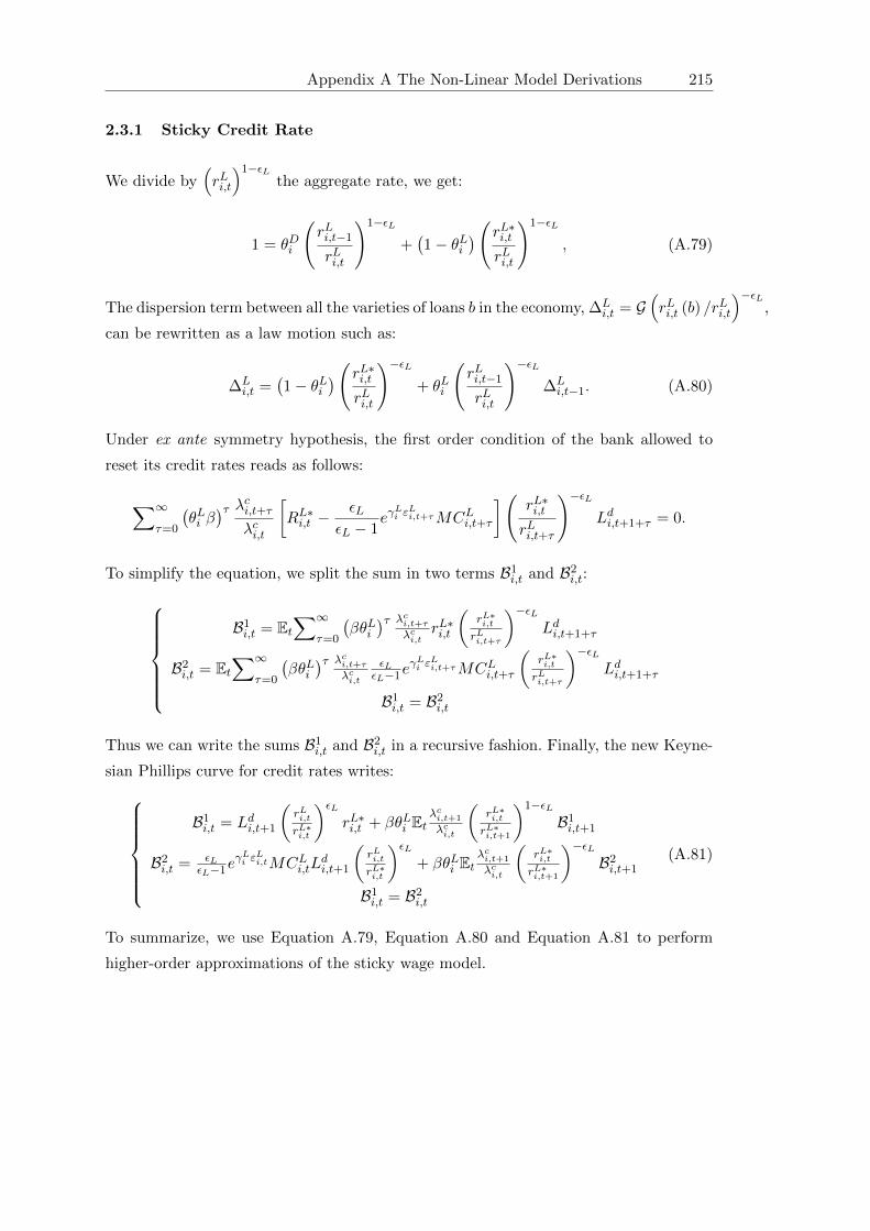
Appendix A The Non-Linear Model Derivations 215
2.3.1 Sticky Credit Rate
We divide by(rLi,t
)1−εLthe aggregate rate, we get:
1 = θDi
(rLi,t−1
rLi,t
)1−εL+(1− θLi
)(rL∗i,trLi,t
)1−εL, (A.79)
The dispersion term between all the varieties of loans b in the economy, ∆Li,t = G
(rLi,t (b) /rLi,t
)−εL,
can be rewritten as a law motion such as:
∆Li,t =
(1− θLi
)(rL∗i,trLi,t
)−εL+ θLi
(rLi,t−1
rLi,t
)−εL∆Li,t−1. (A.80)
Under ex ante symmetry hypothesis, the first order condition of the bank allowed to
reset its credit rates reads as follows:
∑∞τ=0
(θLi β
)τ λci,t+τλci,t
[RL∗i,t −
εLεL − 1
eγLi ε
Li,t+τMCLi,t+τ
](rL∗i,trLi,t+τ
)−εLLdi,t+1+τ = 0.
To simplify the equation, we split the sum in two terms B1i,t and B2
i,t:
B1i,t = Et
∑∞τ=0
(βθLi
)τ λci,t+τλci,t
rL∗i,t
(rL∗i,trLi,t+τ
)−εLLdi,t+1+τ
B2i,t = Et
∑∞τ=0
(βθLi
)τ λci,t+τλci,t
εLεL−1e
γLi εLi,t+τMCLi,t+τ
(rL∗i,trLi,t+τ
)−εLLdi,t+1+τ
B1i,t = B2
i,t
Thus we can write the sums B1i,t and B2
i,t in a recursive fashion. Finally, the new Keyne-
sian Phillips curve for credit rates writes:
B1i,t = Ldi,t+1
(rLi,trL∗i,t
)εLrL∗i,t + βθLi Et
λci,t+1
λci,t
(rL∗i,trL∗i,t+1
)1−εLB1i,t+1
B2i,t = εL
εL−1eγLi ε
Li,tMCLi,tL
di,t+1
(rLi,trL∗i,t
)εL+ βθLi Et
λci,t+1
λci,t
(rL∗i,trL∗i,t+1
)−εLB2i,t+1
B1i,t = B2
i,t
(A.81)
To summarize, we use Equation A.79, Equation A.80 and Equation A.81 to perform
higher-order approximations of the sticky wage model.

216 Appendix A The Non-Linear Model Derivations
2.3.2 Sticky Deposit Rate
We divide by(rDi,t
)1−εD, the aggregate rate writes:
1 = θDi
(rDi,t−1
rDi,t
)1−εD+(1− θDi
)(rD∗i,trDi,t
)1−εD(A.82)
the dispersion term, ∆Di,t = G
(rDi,t(b)
rDi,t
)−εDis defined by:
∆Di,t =
(1− θDi
)(rD∗i,trDi,t
)−εD+ θDi
(rDi,t−1
rDi,t
)−εD∆Di,t−1 (A.83)
Under ex ante symmetry hypothesis, the first order condition of the bank allowed to
reset its deposit rates reads as follows:
∑∞τ=0
(θDi β
)τ λci,t+τλci,t
[rD∗i,t −
εDεD − 1
eγDi ε
Di,t+τMCLi,t+τ
](rD∗i,trDi,t+τ
)−εDLdi,t+1+τ = 0
to simplify the equation, we split the sum:
D1i,t = Et
∑∞τ=0
(βθDi
)τ λci,t+τλci,t
rD∗i,t
(rD∗i,trLi,t+τ
)−εDDdi,t+1+τ ,
D2i,t = Et
∑∞τ=0
(βθDi
)τ λci,t+τλci,t
eγDi ε
Di,t+τ εD
εD−1MCDi,t+τ
(rD∗i,trDi,t+τ
)−εDDdi,t+1+τ ,
D1i,t = D2
i,t.
Thus we can write the sums D1i,t and D2
i,t in a recursive fashion. Finally, the new Key-
nesian Phillips curve for deposit rates writes:
D1i,t = Dd
i,t+1
(rDi,trD∗i,t
)εDRD∗i,t + βθDi Et
λci,t+1
λci,t
(rD∗i,trD∗i,t+1
)1−εDD1i,t+1,
D2i,t = eγ
Di ε
Di,t εDεD−1MCDi,t+τD
di,t+1
(rDi,trD∗i,t
)εD+ βθDi Et
λci,t+1
λci,t
(rD∗i,trD∗i,t+1
)−εDD2i,t+1,
D1i,t = D2
i,t.
(A.84)

Appendix B
The Linear Model
This appendix presents the log-linearized version of the model described in Chapter 2.
We rewrite all the equations in real terms as in open economy model prices posses a
random walk component.
1 Households
Euler Equation 2.13 taken in logs:
σCh(Etch,t+1 −
(1 + hCh
)ch,t + hCh ch,t−1
)=(1− hCh
) (rt − EtπCh,t+1 + εUh,t+1 − εUh,t − CχB bh,t
)
σCf
(Etcf,t+1 −
(1 + hCf
)cf,t + hCf cf,t−1
)=(
1− hCf)(
rt − EtπCf,t+1 + εUf,t+1 − εUf,t + CχB bh,t
) .
(B.1)
The hours supply Equation 2.14 is determined by:
whi,t =1
σLihi,t +
σCi(1− hCi
) (ci,t − hCi ci,t−1
). (B.2)
2 Unions
The staggered real wage equation Equation 2.16 combined with aggregate wage index
equation Equation 2.31 give rise to the new Keynesian Phillips curve for wages:
(1 + β) wi,t = ξWi πCi,t−1 + wi,t−1 −
(1 + βξWi
)πCi,t + βEt
(wi,t+1 + πCi,t+1
)(B.3)
+
(1− βθWi
) (1− θWi
)
θWi
(whi,t − wi,t
).
217

218 Appendix B The Linear Model
3 Firms
The production function in Equation 2.17 writes:
yi,t = εAi,t + αkui,t + (1− α) hi,t. (B.4)
The marginal cost in Equation 2.18 is:
mci,t = αzi,t + (1− α) wi,t − εAi,t, (B.5)
and inputs are linked by:
wi,t + hi,t = kui,t + zi,t. (B.6)
Taking in logs, Equation 2.20 and Equation 2.30 give rise to the new Keynesian Phillips
curve for prices:
(1 + ξPh
)πCh,t = ξPh π
Ch,t−1 + βEtπCh,t+1 +
(1−βθPh )(1−θPh )θPh
(mch,t + αC T oT t
)
(1 + ξPf
)πCf,t = ξPf π
Cf,t−1 + βEtπCf,t+1 +
(1−βθPf )(1−θPf )θPf
(mcf,t − αC T oT t
) . (B.7)
The home final demand in Equation 2.29 is:
yh,t =C
Y
((1− αC
)ch,t + αC cf,t
)+I
Y
((1− αI
)ıh,t + αI ıf,t
)+G
YεGh,t + ZKuh,t (B.8)
+ 2µ
(C
YαC(1− αC
)+I
YαI(1− αI
))T oT t,
and its foreign counterpart:
yf,t =C
Y
((1− αC
)cf,t + αC ch,t
)+I
Y
((1− αI
)ıf,t + αI ıh,t
)+G
YεGf,t + ZKuf,t (B.9)
− 2µ
(C
YαC(1− αC
)+I
YαI(1− αI
))T oT t.
As in Bernanke et al. (1999), we assume that the defaulting share of investment projects
is second order (i.e. we neglect them in our first order approximation of our equilibrium
conditions).
4 Entrepreneurs
The net wealth law of motion in Equation 2.8 writes:
ni,t =(1− τE
) VNvi,t − εNi,t. (B.10)

Appendix B The Linear Model 219
The one-period-profit equation of entrepreneurs reads:
vi,t = (1− κ) (1− κi)ηk
ηk − 1
(qi,t−1 + ki,t−1 − ni,t−1
)+ rki,t + qi,t−1 + ki,t−1, (B.11)
where ηk = N/K. The balance sheet of entrepreneurs in Equation 2.1 is:
(1− ηk
)(ldi,t − hLi ldi,t−1
)+ ηkni,t = qi,t + ki,t. (B.12)
The external premium (or the firm’s spread) in Equation 2.7 is:
si,t = κiηk
ηk − 1
(qi,t + ki,t − ni,t
)+ εQi,t, (B.13)
where:
si,t = Etrki,t+1 − pLi,t. (B.14)
The ex post threshold in Equation 2.5 reads as follows:
ωci,t + rki,t + qi,t−1 + ki,t−1 = pLi,t−1 + ldi,t−1 − hLi ldi,t−2. (B.15)
The expected rate of insolvent investment projects is defined by:
ηEi,t = −κωci,t. (B.16)
5 Banks
Credit market equilibrium from equation writes:
lsh,t =(1− αL
)ldh,t + αL ldf,t + αL2ν
(1− αL
) [rLf,t + πCf,t − rLh,t − πCh,t
]
lsf,t =(1− αL
)ldf,t + αL ldh,t − αL2ν
(1− αL
) [rLf,t + πCf,t − rLh,t − πCh,t
] . (B.17)
The real marginal cost of one unit of loan in Equation 2.33 is defined by:
mcLi,t = κηk
ηk − 1
((1− αL
)(1− κi)
(qi,t + ki,t − ni,t
)+ αL (1− κ−i)
(q−i,t + k−i,t − n−i,t
))
(B.18)
+(rt − Etπci,t+1
).

220 Appendix B The Linear Model
Mixing Equation 2.26 and Equation 2.32 gives rise to the real credit rate dynamic:
rLi,t =1
1 + β(1 + ξLi
)
(1 + ξLi (1 + β)
)rLi,t−1 − ξLi rLi,t−2 + βEtrLi,t+1
+βθLi EtπCi,t+2 −(1 + βθLi
)EtπCi,t+1 + πCi,t
+(1−θLi )(1−θLi β)
θLi
[mcLi,t − rLi,t
]
+ εLi,t, (B.19)
and the banking spread is:
sLi,t = rLi,t −(rt − EtπCi,t+1
). (B.20)
6 Capital Supply Decisions
The ex post return on capital in Equation 2.23 taken in logs becomes:
{Et−1r
kh,t = Z
Rkzh,t + (1−δ)
Rkqh,t − qh,t−1 − εUh,t+1 + εUh,t + C
RkχB bh,t−1
Et−1rkf,t = Z
Rkzf,t + (1−δ)
Rkqf,t − qf,t−1 − εUf,t+1 + εUf,t − C
RkχB bh,t−1
. (B.21)
The law of motion of capital is standard in Equation 2.21 is:
δıi,t = ki,t − (1− δ) ki,t−1, (B.22)
and the capital utilized by the intermediate sector is:
kui,t = ui,t + ki,t−1. (B.23)
The capital utilization rate is:ψi
1− ψiui,t = zi,t (B.24)
the first order condition of capital producers in real terms in Equation 2.22 writes:
{qh,t +
(αC − αI
)T oT t = χIh (ıh,t − ıh,t−1)− βχIh (Etıh,t+1 − ıh,t) ,
qf,t −(αC − αI
)T oT t = χIf (ıf,t − ıf,t−1)− βχIf (Etıf,t+1 − ıf,t) .
(B.25)
7 International Macroeconomics Definitions
Home and foreign consumption price inflation indexes are:
πCh,t = πh,t + αC(T oT t − T oT t−1
),
πCf,t = πf,t − αC(T oT t − T oT t−1
).
(B.26)

Appendix B The Linear Model 221
The credit rate index in real terms is:
pLh,t =(1− αL
)rLh,t + αLrLf,t + αLEt
(πCf,t+1 − πCh,t+1
). (B.27)
From the home country perspective, the terms of trade is:
T oT t = πf,t − πh,t + T oT t−1. (B.28)
The home bonds law of motion:
bh,t − bh,t−1 =C
YαC(cf,t − ch,t +
(2µ(1− αI
)− 1)T oT t
)(B.29)
+I
YαI(if,t − ih,t +
(2µ(1− αC
)− 1)T oT t
).
The home current account dynamic:
cah,t = C(bh,t − bh,t−1
)+ LαL
(RL − 1
) (ldf,t − ldh,t +
(1− 2αC
)T oT t
)(B.30)
+ LαL(RL − 1
) (2ν(1− αL
)− 1) (rLf,t + πCf,t − rLh,t − πCh,t
).
8 Monetary Policy
And finally, the Taylor rules follows the law of motion in Equation 2.28:
rt = ρRrt−1 +1
2
(1− ρR
) [φπ(πCh,t + πCf,t
)+ φ∆y (yh,t − yh,t−1 + yf,t − yf,t−1)
]+ ηRt .
(B.31)
9 Shocks Processes
The shock processes are defined by:
εAi,t = ρAi εAi,t−1 + ηAi,t, (B.32)
εGi,t = ρGi εGi,t−1 + ηGi,t, (B.33)
εUi,t = ρUi εUi,t−1 + ηUi,t, (B.34)
εQi,t = ρQi εQi,t−1 + ηQi,t, (B.35)
εNi,t = ρNi εNi,t−1 + ηNi,t, (B.36)
εLi,t = ρLi εLi,t−1 + ηLi,t. (B.37)


Appendix C
Additional Quantitative Results
This appendix presents some additional results that are not necessary for the analysis of
macroprudential policy and cross-border lending. We develop a model with quantitative
properties similar to Smets & Wouters (2003) in a two-country perspective augmented
with an international banking system that considers the short-run divergences in the
business cycles of the Eurozone.
This appendix is organized as follows: Section 1 presents the prediction performances
of the Chapter 4 estimated model. Section 2 presents the driving forces of the busi-
ness cycles since the Eurosystem creation. Section 3 evaluates the robustness of our
quantitative exploration to the zero lower bound. Section 4 examines the historical
decomposition of business and credit cycles.
1 Empirical Performances
While obtaining the highest possible data fit was not the primary objective of building
our model, it may be useful to take a close look at the forecasting performance of the
model. Figure C.1 presents a simple tool to assess the empirical performance of a DSGE
model, that consists in casting its one-side Kalman filter predictions of the observable
variables against their realizations. The Kalman filter generates projections or forecasts
of the state of the linear approximate solution of the DSGE model given an information
set of observed macro time series (see for instance Guerron-Quintana & Nason (2012)
for more informations). Thus, we can compare the prediction performances of output,
consumption, inflation, investment, loan supply, credit rates, interbank supply, real
wages and ECB refinancing rate.
Overall, our model does a good job at tracking the main variables of the Euro Area with
some noticeable exceptions:
223

224 Appendix C Additional Quantitative Results
2000 2002 2004 2006 2008 2010 2012
−2
0
2
Core ∆ log Production
2000 2002 2004 2006 2008 2010 2012
−2
0
Periph. ∆ log Production
2000 2002 2004 2006 2008 2010 2012
0
2
Core ∆ log Consommation
2000 2002 2004 2006 2008 2010 2012
−2
0
2
Periph. ∆ log Consommation
2000 2002 2004 2006 2008 2010 2012−1
−0.5
0
0.5
Core ∆ log CPI
2000 2002 2004 2006 2008 2010 2012−1
−0.5
0
0.5
Periph. ∆ log CPI
2000 2002 2004 2006 2008 2010 2012
−10
−5
0
5
Core ∆ log Investment
2000 2002 2004 2006 2008 2010 2012
−5
0
Periph. ∆ log Investment
2000 2002 2004 2006 2008 2010 2012−2
0
2
Core ∆ log Loan Supply
2000 2002 2004 2006 2008 2010 2012−4
−2
0
2
4
Periph. ∆ log Loan Supply
2000 2002 2004 2006 2008 2010 2012
−2
0
2
∆Core Credit Rate
2000 2002 2004 2006 2008 2010 2012
−2
0
2
∆Periph. Credit Rate
2000 2002 2004 2006 2008 2010 2012
−5
0
5
∆Core ∆ log Interbank Loans
2000 2002 2004 2006 2008 2010 2012
−5
0
5
∆Periph. ∆ log Interbank Loans
2000 2002 2004 2006 2008 2010 2012−2
0
2
Core ∆ log Real Wages
2000 2002 2004 2006 2008 2010 2012
−1
0
1
2
Periph. ∆ log Real Wages
2000 2002 2004 2006 2008 2010 2012−2
0
2
ECB Refinancing Rate
One-step-ahead forecastData
Figure C.1: Data and one-step-ahead forecasts generated from Chapter 4 model.

Appendix C Additional Quantitative Results 225
First, the model does not capture the volatility in real wage growth. This issue may be
solved by replacing the labour supply equation (i.e. the households marginal utility of
labour) and the sticky wage model with a better micro-founded labor market friction
such as from search-matching models a la Christiano et al. (2011).
Second, the model clearly fails at explaining the pre-crisis credit boom for firms in core
countries as well as the after-crisis sharp drop in the credit supply from the core banking
system. To enhance the forecasting performances of the credit supply in the core area,
a more sophisticated bank balance sheet that incorporates housing loans and sovereign
bonds could help in catching up these aggregate fluctuations.
In addition, the model performs well at predicting core countries consumption fluctua-
tions but not its volatility size. This failure on consumption has a clear side-effect on the
output growth prediction. This problem regarding consumption forecasting is probably
related to the real wage growth prediction.
Altogether, the overall in-sample fit of our model seems to be acceptable if one takes
into account a highly restrictive nature of the DSGE framework.
2 Driving Forces of Output
As Smets & Wouters (2007), we can study the driving force of output in the Euro
Area since its creation in 1999. In Figure C.2, we plot the forecast variance error
decomposition of output in core and peripheral areas. All the shocks are gathered
according to their type: Supply (ηAi,t); Demand (ηGi,t and ηUi,t); Financial (ηQi,t, ηNi,t, η
Li,t
and ηBi,t and the common shocks); Wage mark-up (ηWi,t ) and Monetary policy (ηRt ).
First, two areas are pretty similar in the forces that drive output fluctuations in the
sample period either in the short and in the long run. Supply shocks accounts for about
20% to 35% of business cycles variations. This result is comparable to the Smets &
Wouters (2007)’s findings for the US economy. On the other hand, demand shocks
only account for 10% of output variations, they are replaced by financial shocks, which
appear to be the main drivers of the Euro Area business cycles. This result is not
surprising, as banking shocks had a very important role in fuelling the propriety boom
followed by a bust cycle, justifying the need for macroprudential measures. In the short
run (i.e. within a year), real GDP is primarily driven by supply shocks which affects
the production function and prices in the Eurozone. In the long run (more than 40
quarters), supply shocks are slightly replaced by financial shocks. In comparison, wage
mark-up shocks remain pretty constant over the forecasting horizon.

226 Appendix C Additional Quantitative Results
Q1 Q2 Q4 Q10 Q40 Q100
0
20
40
60
80
100
Core GDP Growth ∆yc,t
Q1 Q2 Q4 Q10 Q40 Q100
0
20
40
60
80
100
Periph. GDP Growth ∆yp,t
Supply DemandFinancial Wage Mark-upMonetary Policy
Figure C.2: Forecast error variance decomposition of GDP growth at the mean ofthe posterior distribution generated by the model in Chapter 4.

Appendix C Additional Quantitative Results 227
3 Robustness Check to the Zero Lower Bound
In the quantitative simulations of Chapter 3 and Chapter 5, we performed monetary
policy coefficients optimization exercises without considering the perspective of hitting
the zero lower bound (ZLB). In DSGE models, the zero lower bound has initially been
addressed by McCallum (2000) and Woodford (2002). In our simulations, we optimize
the policy coefficient on inflation using a welfare criterion in Chapter 5, given our grid
search φπ ∈ [1, 3] we found that the optimal parameter that penalizes inflation is φπ = 3,
which is higher than the estimated coefficient. A high value of φπ increases the volatility
of the nominal interest rate and, in turn, increases the probability of violating the zero
lower bound.
In this section, we check whether the model conclusions rely on realistic scenarios by
computing the ZLB probability. To do so, we first consider the estimated model in
Chapter 5 and generate artificial series for the Euro area given the estimated standard
deviations of shocks. As example, in Figure C.3, we generate 110 draws of the ECB
nominal interest rate and we neglect the first 10 draws. As observed, with high value
of φπ, the probability to violate the zero lower bound increases as the interest rate
approaches zero. For the estimated and the optimized scenarios, the interest rates
remain far from zero.
To get the probability of hitting the zero lower bound using the model asymptotic
properties, we generate a larger sample of 1,000 draws and we compute the number of
times the interest rate is below 0. To compute a confidence interval, we reiterate the
operation 100 times. Finally, we do this exercise for various values of φπ.
Figure C.4 reports the results. We find that on policy coefficients lying in the interval
(1, 3] for φπ is relevant as the ZLB is clearly below 2%, which is faily low. Considering a
larger grid search interval could lead to fallacious results. For instance, Quint & Rabanal
(2013) explore monetary policy coefficients in the interval (1, 5] without computing the
zero lower bound probability, this could lead to fallacious results in terms of welfare
ranking of alternative implementation schemes. In the same vein, Darracq-Paries et al.
(2011) consider wider intervals for monetary policy coefficients than Quint & Rabanal
(2013) and they probably face a ZLB probability higher than 20% in their quantitative
simulations.

228 Appendix C Additional Quantitative Results
0 10 20 30 40 50 60 70 80 90 100
1
2
3
anchorφπ = 1.6 and φ∆y = 0.20 (estimated)anchorφπ = 3 and φ∆y = 0 (optimized)anchorφπ = 10 and φ∆y = 0 (counterfactual)
Figure C.3: ECB nominal interest rate simulated by the model of Chapter 5.
1 2 3 4 5 6 7 8 9 100
5
10
15
20
Inflation Penalization φπ
%
anchorZLB probabilityanchor90% Interval
Figure C.4: Zero lower bound probability for various values of the monetary policyreaction parameter to inflation generated by the model of Chapter 5.

Appendix C Additional Quantitative Results 229
4 Historical Decomposition of Business and Credit Cycles
in the UEM
In Figure C.5 and Figure C.6, we perform an historical decomposition of the dynamics
of the four main variables of interest (activity, inflation, corporate and interbank loan
supplies) as in Smets & Wouters (2007). The aim of the exercise is to investigate the
consequences of the financial crisis of 2007 on the driving forces of activity, investment
and corporate and interbank loan supplies. We plot the same figure as Smets & Wouters
(2007): we gather the shocks in five groups: supply (productivity), demand (investment
costs, spending and preferences), financial (deposit and credit rates mark-ups, collat-
eral crunch, bank liabilities crunch), monetary policy and mark-ups (inflation and real
wages).
In Figure C.5, we observe that the financial crisis episode was triggered by a demand
shock followed by persistent financial shocks for core countries. The story is different for
peripheral countries as the financial turmoil started with large and persistent financial
shocks. The model also catches up the fiscal consolidation period after 2011 via a slow-
down in the positive contribution of demand shocks. Financial shocks have a significant
impact on inflation fluctuations in core countries inflation fluctuations. In this environ-
ment, monetary and macroprudential policies can play a major role in dampening such
macroeoconomic developments. Turning to peripheral countries, we get the same kind
of result during the post crisis period: the deflation that hits peripheral countries is
explained by the model by depressed and persistent financial cycles.
Figure C.6 reports financial cycles (corporate and interbank loan supplies in the two
regions). Remarkably, corporate loan cycles are mainly driven by financial shocks. We
observe that the the financial crisis episode was triggered by a demand shock followed
by persistent financial shocks for core countries. Volatility is much higher for peripheral
countries. Postcrisis developments a clearly impacted by the curative measures under-
taken in this area. The picture for interbank loans is a bit different, as demand shocks
play an important role in the observed fluctuations of this varible in both parts of the
Eurozone. This feature can be link to the household preference shock that increases
saving, and conversely, the size of deposit in the banking system. As banks are capital
constrained, the balance sheet of this agent plays an important role on macroeocnomic
developments. One interesting feature observed is that the US subprime crisis depressed
interbank supply one year before the beginning of Eurozone economic slump. This kind
of result underlines the interest of focussing the interbank loan developements as an
early warning signal of a forthcoming crisis event.

230 Appendix C Additional Quantitative Results
2000 2002 2004 2006 2008 2010 2012−4 %
−2 %
0 %
2 %log ∆yc,t GDP Growth in Core Countries
2000 2002 2004 2006 2008 2010 2012
−2 %
0 %
2 %log ∆yp,t GDP Growth in Peripheral Countries
2000 2002 2004 2006 2008 2010 2012
−0.5 %
−0.25 %
0 %
0.25 %
0.5 %
log ∆πCc,t Inflation in Core Countries
2000 2002 2004 2006 2008 2010 2012
−0.75 %−0.5 %−0.25 %
0 %0.25 %0.5 %
0.75 %
log ∆πCp,t Inflation in Peripheral Countries
Supply Demand FinancialMark-up Monetary Policy ResidualData
Figure C.5: The historical decomposition of output and inflation generated by themodel in Chapter 5.

Appendix C Additional Quantitative Results 231
2000 2002 2004 2006 2008 2010 2012
−2 %
0 %
2 %
log ∆lsc,t Corporate Loan Supply Growth in Core Countries
2000 2002 2004 2006 2008 2010 2012−6 %
−4 %
−2 %−1 %
0 %1 %2 %3 %4 %
log ∆lsp,t Corporate Loan Supply Growth in Peripheral Countries
2000 2002 2004 2006 2008 2010 2012
−6 %
−4 %
−2 %
0 %
2 %
4 %
6 %
8 %log ∆ibc,t Interbank Loan Supply Growth in Core Countries
2000 2002 2004 2006 2008 2010 2012
−10 %−8 %−6 %−4 %−2 %
0 %2 %4 %6 %8 %
10 %log ∆ibp,t Interbank Loan Supply Growth in Peripheral Countries
Supply Demand FinancialMark-up Monetary Policy ResidualData
Figure C.6: The historical decomposition of corporate and interbank credit supplygenerated by the model in Chapter 5.


List of Figures
1 Boom and bust cycles in the Eurozone (millions of euro per capita, sourcesECB). . . . . . . . . . . . . . . . . . . . . . . . . . . . . . . . . . . . . . 2
2 GDP Loss after the financial crisis episode in the Eurozone and the US(Sources FRED). . . . . . . . . . . . . . . . . . . . . . . . . . . . . . . . 2
3 Globalization of banks balance sheet in Europe and abroad since 1999(Sources BIS ). . . . . . . . . . . . . . . . . . . . . . . . . . . . . . . . . 7
4 Share of cross-border loans (by loan type) between EMU participants inthe assets of core and peripheral banks of the Eurosystem. (Sources: ECB) 8
5 Structural divergences in the supply of loans before the financial crisisepisode (per capita million euro, sources Eurostats) . . . . . . . . . . . . 9
6 Regional divergences and their implications for the implementation of anhomogenous macroprudential policy (sources Eurostats). . . . . . . . . . 9
1.1 Output and loan costs after the 2007 financial crisis episode for the USeconomy.Sources: FRED database. . . . . . . . . . . . . . . . . . . . . . . . . . . 20
1.2 A comparison of supply and demand shocks effects with and withoutfinancial frictions . . . . . . . . . . . . . . . . . . . . . . . . . . . . . . . 25
1.3 Welfare loss for different values of λπ with Cooperative and Nash imple-mentations. . . . . . . . . . . . . . . . . . . . . . . . . . . . . . . . . . . 36
2.1 Evolution et tensions du secteur bancaire depuis la creation de l’euro. . 40
2.2 Le modele d’une union monetaire a deux pays avec des prets transfrontaliers 41
2.3 IRF bayesienne des modeles M2 avec prets transfrontaliers (en lignepleine) et M1 sans (en pointilles) suite a un choc positif de productiviteet de destruction d’actifs financiers en Allemagne . . . . . . . . . . . . . 57
3.1 Stylized facts characterizing the Eurosystem banking system: credit cy-cles remain clearly national while cross-border lending experienced anexplosive growth (ESRB and BIS statistics). . . . . . . . . . . . . . . . . 62
3.2 The model of monetary union with cross-border lending facilities. . . . . 66
3.3 Observable variables . . . . . . . . . . . . . . . . . . . . . . . . . . . . . 80
3.4 Historical contributions to Investment (year-on-year % change generatedby the model). . . . . . . . . . . . . . . . . . . . . . . . . . . . . . . . . 85
3.5 Prior and posterior distributions of parameters. . . . . . . . . . . . . . . 86
3.6 Dynamic correlations of the main variables: observable variables (blue)and 90% confidence band interval generated by the estimated model cen-tered around the asymptotic mean . . . . . . . . . . . . . . . . . . . . . 88
233

List of Figures
3.7 Counterfactual paths of investment (million euro) under different optimalimplementation schemes: no macroprudential policy (green crossed), co-ordinated macroprudential policy (red circled), Non coordinated macro-prudential policy - Host principle (blue dashed) and Non coordinatedmacroprudential policy - Home principle (black dotted), and the CEPRRecession Indicator for Euro Area Business Cycles (shaded area). . . . . 94
3.8 The financial crisis episode: system response after simulating the financialcrisis (2009Q1 shocks) under the optimal policy regime and the optimalcoordinated macroprudential policy. . . . . . . . . . . . . . . . . . . . . 96
4.1 Internationalization of credit markets in the Eurozone and abroad be-tween 1999 and 2013 (Sources ECB, BIS ) . . . . . . . . . . . . . . . . . 102
4.2 Share of Cross-Border Loans between EMU participants in the assets ofCore and Peripheral Banks . . . . . . . . . . . . . . . . . . . . . . . . . 103
4.3 The model of a two-country monetary union with international bank loanflows . . . . . . . . . . . . . . . . . . . . . . . . . . . . . . . . . . . . . . 105
4.4 Observable variables used in the estimation . . . . . . . . . . . . . . . . 121
4.5 The priors and posteriors distributions of the model parameters withcross-border banking flows. . . . . . . . . . . . . . . . . . . . . . . . . . 126
4.6 Bayesian system response to an estimated positive productivity shock incore countries under banking globalization (αL = 9%, αIB = 11%) andautarky (αL = αIB = 0%) . . . . . . . . . . . . . . . . . . . . . . . . . . 128
4.7 Bayesian system response to an estimated negative net wealth shock incore countries under banking globalization (αL = 9%, αIB = 11%) andautarky (αL = αIB = 0%) . . . . . . . . . . . . . . . . . . . . . . . . . . 132
4.8 Bayesian system response to an estimated positive liability shock in thebalance sheet of core countries banks under banking globalization (αL =9%, αIB = 11%) and autarky (αL = αIB = 0%) . . . . . . . . . . . . . 134
4.9 The peripheral current account (quarter-on-quarter % change generatedby the model with cross-border flows).Note:The solid blue line depicts the quarterly growth rate in real GDP andInvestment (per capita), expressed in percentage point deviations fromthe model’s steady state. The colored bars depict the estimated contri-butions of the various groups of shocks (Real and Nominal:productivity,wage cost-push, spending, preferences asymmetric shocks; Financial:externalfinance premium, credit cost push, net worth and liabilities asymmetricshocks; Common Financial:external finance premium, credit cost push,net worth, bank liabilities and monetary policy common shocks. . . . . . 141
4.10 The system response during the financial crisis (2009Q1) under differentlevels of financial openness . . . . . . . . . . . . . . . . . . . . . . . . . . 142
5.1 Regional divergences in the UEM . . . . . . . . . . . . . . . . . . . . . . 147
5.2 Road map of the newly created institutions in the European Union . . . 148
5.3 Recommendation of the European Systemic Risk Board of 4 April 2013on intermediate objectives and instruments of macro-prudential policy(ESRB/2013/1) . . . . . . . . . . . . . . . . . . . . . . . . . . . . . . . . 149
5.4 The model of a two-country monetary union with international bank loanflows . . . . . . . . . . . . . . . . . . . . . . . . . . . . . . . . . . . . . . 150
5.5 Observable variables . . . . . . . . . . . . . . . . . . . . . . . . . . . . . 153

List of Figures LIST OF FIGURES 235
5.6 Prior and posterior distributions of parameters. . . . . . . . . . . . . . . 157
5.7 Dynamic correlations of the main variables: observable variables (blue)and 90% confidence band interval generated by the estimated model cen-tered around the asymptotic mean . . . . . . . . . . . . . . . . . . . . . 162
A.1 The role of sticky wages in matching the business cycles of the Euro Area(generated from chapter 4 model). . . . . . . . . . . . . . . . . . . . . . 182
A.2 Implementing the financial accelerator in a real business cycle model . . 184
A.4 The role of sticky prices in matching the business cycles of the Euro Area(generated from chapter 4 model). . . . . . . . . . . . . . . . . . . . . . 186
A.3 Profit sharing between the entrepreneur and the bank (in chapter 2 and4, µB = 1). . . . . . . . . . . . . . . . . . . . . . . . . . . . . . . . . . . 187
A.5 Pareto distribution of heterogenous entrepreneurs’ projects ω ∈ [ωmin,+∞[. . . . . . . . . . . . . . . . . . . . . . . . . . . . . . . . . . . . . . . . . 187
A.6 The role of loan demand habits in matching the business cycles of theEuro Area (generated from chapter 5 model). . . . . . . . . . . . . . . . 188
A.7 The role of the financial accelerator in matching the business cycles ofthe Euro Area (generated from chapter 4 model). . . . . . . . . . . . . . 192
A.8 The role of investment adjustment costs in matching the business cyclesof the Euro Area (generated from chapter 4 model). . . . . . . . . . . . . 194
A.9 The role of variable capital utilization in matching the business cycles ofthe Euro Area (generated from chapter 4 model). . . . . . . . . . . . . . 196
A.10 Implementing the interbank market in a New Keynesian Framework . . 198
A.11 The role of an heterogenous banking system in matching the businesscycles of the Euro Area (generated from chapter 4 model). . . . . . . . . 204
A.12 The role of sticky credit rates in matching the business cycles of the EuroArea (generated from chapter 5 model). . . . . . . . . . . . . . . . . . . 206
A.13 The role of sticky deposit rates in matching the business cycles of theEuro Area (generated from chapter 5 model). . . . . . . . . . . . . . . . 208
C.1 Data and one-step-ahead forecasts generated from Chapter 4 model. . . 224
C.2 Forecast error variance decomposition of GDP growth at the mean of theposterior distribution generated by the model in Chapter 4. . . . . . . . 226
C.3 ECB nominal interest rate simulated by the model of Chapter 5. . . . . 228
C.4 Zero lower bound probability for various values of the monetary policyreaction parameter to inflation generated by the model of Chapter 5. . . 228
C.5 The historical decomposition of output and inflation generated by themodel in Chapter 5. . . . . . . . . . . . . . . . . . . . . . . . . . . . . . 230
C.6 The historical decomposition of corporate and interbank credit supplygenerated by the model in Chapter 5. . . . . . . . . . . . . . . . . . . . 231


List of Tables
1.1 Diffusion of supply and demand shocks with and without financial fric-tions. . . . . . . . . . . . . . . . . . . . . . . . . . . . . . . . . . . . . . 24
1.2 Model response to a cost push shock εS under optimal monetary policywith and without a financial concern. . . . . . . . . . . . . . . . . . . . 28
1.3 A comparison of the Nash and cooperative equilibriums . . . . . . . . . 32
2.1 Distributions des croyances a priori et des a posteriori des parametresstructurels et des processus de choc. . . . . . . . . . . . . . . . . . . . . . . . . . . . . . . . . . . . . . . . . 54
2.2 Decomposition de la variance inconditionnelle a posteriori en % : elle estla part en % de variance expliquee par chaque choc selon le modele M1
(sans prets transfrontaliers) et M2 (avec). CAall est le compte courantallemand (sachant que CAall = −CAfr). . . . . . . . . . . . . . . . . . 59
3.1 Different levels of implementation of Macroprudential policy . . . . . . 73
3.2 Calibration of the model (all parameters are on a quarterly basis) . . . 81
3.3 Prior and Posterior distributions of structural parameters and shock pro-cesses. . . . . . . . . . . . . . . . . . . . . . . . . . . . . . . . . . . . . . 83
3.4 Empirical and Theoretical Standard deviations . . . . . . . . . . . . . . 85
3.5 Welfare-based Performance of Macroprudential Rules . . . . . . . . . . 91
3.6 Standard deviation of model generated investment under different imple-mentation schemes . . . . . . . . . . . . . . . . . . . . . . . . . . . . . . 95
4.1 Calibration of the model (all parameters are quarterly) . . . . . . . . . 122
4.2 Prior and Posterior distributions of shock processes . . . . . . . . . . . 123
4.3 Prior and Posterior distributions of structural parameters . . . . . . . . 124
4.4 Prior and posterior model probabilities . . . . . . . . . . . . . . . . . . 125
4.5 The unconditional variance decomposition is the share of variance ac-counted for by each shock of the model estimated with and without cross-border flows.Note:Supply: productivity (ηAi,t) and wage cost-push (ηWi,t ); Demand: pref-
erences (ηβi,t) and spending (ηGi,t); Financial: collateral (ηNi,t), riskiness (ηQi,t)
credit rate cost-push (ηLi,t), and liabilities (ηBi,t); Common financial: collat-
eral (ηNt ) riskiness (ηQt ) rate cost-push (ηLt ), liabilities (ηBt ) and monetarypolicy (ηRt ). . . . . . . . . . . . . . . . . . . . . . . . . . . . . . . . . . . 136
5.1 Calibration of the model (all parameters are on a quarterly basis). Note:A term denotes the assets of the bank, it is Ls for illiquid banks and¯IBs
+ Ls for liquid ones. . . . . . . . . . . . . . . . . . . . . . . . . . . 155
237

List of Tables
5.2 Prior and Posterior distributions of shock processes . . . . . . . . . . . 158
5.3 Prior and Posterior distributions of structural parameters and shock pro-cesses. Note: IG denotes the Inverse Gamma distribution, B the Beta,N the Normal, G the Gamma. . . . . . . . . . . . . . . . . . . . . . . . 160
5.4 Empirical and Theoretical Standard deviations . . . . . . . . . . . . . . 161
5.5 Homogenous/heterogenous practices in the conduct of MacroprudentialPolicy between different areas in the Euro Area: Nash equilibrium payoffsmatrix in terms of unconditional consumption gains from leaving thestandard optimal monetary policy. . . . . . . . . . . . . . . . . . . . . . 167
5.6 National macroprudential policy coordination dilemma: Nash Equilib-rium Payoffs Matrix (in terms of unconditional consumption gains fromleaving the simple optimal policy) . . . . . . . . . . . . . . . . . . . . . 167
5.7 Macroeconomic performances of different policy regimes . . . . . . . . . 168
5.8 Homogenous/heterogenous practices in the conduct of MacroprudentialPolicy between different areas in the Euro Area in banking autarky: Nashequilibrium payoffs matrix in terms of unconditional consumption gainsfrom leaving the standard optimal monetary policy. . . . . . . . . . . . 174
5.9 National macroprudential policy coordination dilemma in banking au-tarky: Nash Equilibrium Payoffs Matrix (in terms of unconditional con-sumption gains from leaving the simple optimal policy) . . . . . . . . . 174

References
Adjemian, S., Bastani, H., Juillard, M., Mihoubi, F., Perendia, G., Ratto, M., & Ville-
mot, S. (2011). Dynare: Reference manual, version 4. Dynare Working Papers,
1 .
Adjemian, S., Darracq Paries, M., & Smets, F. (2008). A quantitative perspective on
optimal monetary policy cooperation between the us and the euro area.
An, S., & Schorfheide, F. (2007). Bayesian analysis of dsge models. Econometric reviews,
26 (2-4), 113–172.
Andrle, M. (2010). A note on identification patterns in dsge models (Tech. Rep.).
European Central Bank Frankfurt.
Angelini, P., Neri, S., & Panetta, F. (2012). Monetary and macroprudential policies.
Angeloni, I., & Faia, E. (2013). Capital regulation and monetary policy with fragile
banks. Journal of Monetary Economics, 60 (3), 311–324.
Bachmann, R., & Elstner, S. (2013). Firms optimism and pessimism (Tech. Rep.).
National Bureau of Economic Research.
Bailliu, J., Meh, C. A., & Zhang, Y. (2012). Macroprudential rules and monetary policy
when financial frictions matter. Bank of Canada.
Beau, D., Clerc, L., & Mojon, B. (2012). Macro-prudential policy and the conduct of
monetary policy. Banque de France.
Benes, J., & Kumhof, M. (2011). Risky bank lending and optimal capital adequacy
regulation. International Monetary Fund.
Benes, J., Kumhof, M., & Laxton, D. (2014). Financial crises in dsge models: A
prototype model.
Benigno, P., & Woodford, M. (2005). Inflation stabilization and welfare: The case
of a distorted steady state. Journal of the European Economic Association, 3 (6),
1185–1236.
239

Bibliography
Bernanke, B., & Gertler, M. (1989). Agency costs, net worth, and business fluctuations.
American Economic Review , 79 (1), 14–31.
Bernanke, B., Gertler, M., & Gilchrist, S. (1999). The financial accelerator in a quan-
titative business cycle framework. Handbook of macroeconomics, 1 , 1341–1393.
Blanchard, O. J., Dell’Ariccia, M. G., & Mauro, M. P. (2013). Rethinking macro policy
ii: getting granular. International Monetary Fund, Staff Discussion Note, 13 (3).
Bofinger, P., Mayer, E., & Wollmershauser, T. (2006). The bmw model: a new frame-
work for teaching monetary economics. The Journal of Economic Education, 37 (1),
98–117.
Brooks, S., & Gelman, A. (1998). General methods for monitoring convergence of
iterative simulations. Journal of computational and graphical statistics, 7 (4), 434–
455.
Brunnermeier, M., De Gregorio, J., Eichengreen, B., El-Erian, M., Fraga, A., & Ito,
T. (2012). Banks and cross-border capital flows: Policy challenges and regulatory
responses. Brookings Committee on International Economic Policy and Reform.
Brzoza-Brzezina, M., Kolasa, M., & Makarski, K. (2013). Macroprudential policy in-
struments and economic imbalances in the euro area (Tech. Rep.).
Buttet, S., & Roy, U. (2014). A simple treatment of the liquidity trap for intermediate
macroeconomics courses. The Journal of Economic Education, 45 (1), 36–55.
Calvo, G. (1983). Staggered prices in a utility-maximizing framework. Journal of
monetary Economics, 12 (3), 383–398.
Carboni, G., Darracq Paries, M., & Kok Sorensen, C. (2013). Exploring the nexus
between macro-prudential policies and monetary policy measures: Evidence from an
estimated dsge model for the euro area. Becker Friedman Institute for Research in
Economics Working Paper(2013-005).
Casares, M., & Poutineau, J.-C. (2011). Short-run and long-run effects of banking in a
new keynesian model. The BE Journal of Macroeconomics, 11 (1).
Cecchetti, S., & Kohler, M. (2012). When capital adequacy and interest rate policy are
substitutes (and when they are not). Bank for International Settlements, Working
Paper , 379 .
Cecchetti, S., & Li, L. (2008). Do capital adequacy requirements matter for monetary
policy? Economic Inquiry , 46 (4), 643–659.

Bibliography REFERENCES 241
Christiano, L., Eichenbaum, M., & Evans, C. (2005). Nominal rigidities and the dynamic
effects of a shock to monetary policy. Journal of political Economy , 113 (1), 1–45.
Christiano, L., Motto, R., & Rostagno, M. (2009). Financial factors in economic
fluctuations (preliminary) (Tech. Rep.). Citeseer.
Christiano, L., Motto, R., & Rostagno, M. (2010). Financial factors in economic fluc-
tuations.
Christiano, L., Trabandt, M., & Walentin, K. (2011). Introducing financial frictions and
unemployment into a small open economy model. Journal of Economic Dynamics and
Control , 35 (12), 1999–2041.
Clarida, R., Galı, J., & Gertler, M. (1999). The science of monetary policy: a new
keynesian perspective (Tech. Rep.). National Bureau of Economic Research.
Collard, F., Dellas, H., Diba, B., & Loisel, O. (2012). Optimal monetary and prudential
policies. Banque de France.
Crockett, A. (2000). Marrying the micro-and macro-prudential dimensions of financial
stability. BIS speeches, 21 .
Curdia, V., & Woodford, M. (2010). Credit spreads and monetary policy. Journal of
Money, Credit and Banking , 42 , 3–35.
Darracq-Paries, M., Kok-Sørensen, C., & Rodriguez-Palenzuela, D. (2011). Macroeco-
nomic propagation under different regulatory regimes: Evidence from an estimated
dsge model for the euro area. International Journal of Central Banking , 7 (4), 49–113.
Dedola, L., Karadi, P., & Lombardo, G. (2013). Global implications of national uncon-
ventional policies. Journal of Monetary Economics, 60 (1), 66–85.
Dedola, L., & Lombardo, G. (2012). Financial frictions, financial integration and the
international propagation of shocks. Economic Policy , 27 (70), 319–359.
De Graeve, F. (2008). The external finance premium and the macroeconomy: Us post-
wwii evidence. Journal of Economic Dynamics and Control , 32 (11), 3415–3440.
De Grauwe, P. (2010). The scientific foundation of dynamic stochastic general equilib-
rium (dsge) models. Public choice, 144 (3-4), 413–443.
De Larosiere, J. (2009). The high-level group on financial supervision in the eu: report.
European Commission.
De Paoli, B., & Paustian, M. (2013). Coordinating monetary and macroprudential
policies. Federal Reserve Bank of New York, Staff Report , 653 .

Bibliography
Dib, A. (2010). Banks, credit market frictions, and business cycles (Tech. Rep.). Bank
of Canada Working Paper.
Drehmann, M., & Tsatsaronis, K. (2014). The credit-to-gdp gap and countercyclical
capital buffers: questions and answers1. International banking and financial market
developments, 3 , 55.
Eyquem, A., & Poutineau, J.-C. (2010). Markets integration and macroeconomic dis-
persion in a monetary union. Louvain Economic Review , 76 (1), 5–30.
Faia, E. (2007). Finance and international business cycles. Journal of Monetary Eco-
nomics, 54 (4), 1018–1034.
Faia, E., & Iliopulos, E. (2011). Financial openness, financial frictions and optimal
monetary policy. Journal of Economic Dynamics and Control , 35 (11), 1976–1996.
Fatas, A., & et al. (2009). Lessons for monetary policy from asset price fluctuations.
Flagship report on macroprudential policy in the banking sector. (2014).
Forster, K., Vasardani, M., & Zorzi, C. (2011). Euro area cross-border financial flows
and the global financial crisis. (126).
Friedman, B. (2013). The simple analytics of monetary policy: A post-crisis approach
(Tech. Rep.). National Bureau of Economic Research.
Galati, G., & Moessner, R. (2013). Macroprudential policy–a literature review. Journal
of Economic Surveys, 27 (5), 846–878.
Gelain, P., Lansing, K. J., & Mendicino, C. (2012). House prices, credit growth, and
excess volatility: Implications for monetary and macroprudential policy. International
Journal of Central Banking .
Gerali, A., Neri, S., Sessa, L., & Signoretti, F. (2010). Credit and banking in a dsge
model of the euro area. Journal of Money, Credit and Banking , 42 (s1), 107–141.
Gertler, M., & Karadi, P. (2011). A model of unconventional monetary policy. Journal
of Monetary Economics, 58 (1), 17–34.
Gertler, M., & Karadi, P. (2012). A framework for analyzing large scale asset purchases
as a monetary policy tool*.
Gilchrist, S., Ortiz, A., & Zakrajsek, E. (2009). Credit risk and the macroeconomy:
Evidence from an estimated dsge model. Unpublished manuscript, Boston University .
Gilchrist, S., Sim, J., & Zakrajsek, E. (2009). Uncertainty, credit spreads, and investment
dynamics (Tech. Rep.). Boston University mimeo.

Bibliography REFERENCES 243
Goodfriend, M., & King, R. (1997). The new neoclassical synthesis and the role of
monetary policy. , 231–296.
Goodfriend, M., & McCallum, B. (2007). Banking and interest rates in monetary
policy analysis: A quantitative exploration. Journal of Monetary Economics, 54 (5),
1480–1507.
Goodhart, C. A., Sunirand, P., & Tsomocos, D. P. (2005). A risk assessment model for
banks. Annals of Finance, 1 (2), 197–224.
Gray, S., Chailloux, A., & McCaughrin, R. (2008). Central bank collateral frameworks:
Principles and policies. IMF Working Papers, 1–67.
Guerrieri, L., Iacoviello, M., & Minetti, R. (2012). Banks, sovereign debt and the
international transmission of business cycles.
Guerron-Quintana, P. A., & Nason, J. M. (2012). Bayesian estimation of dsge models.
Hirakata, N., Sudo, N., & Ueda, K. (2009). Chained credit contracts and financial
accelerators (Tech. Rep.). Institute for Monetary and Economic Studies, Bank of
Japan.
Hirakata, N., Sudo, N., & Ueda, K. (2011). Do banking shocks matter for the us
economy? Journal of Economic Dynamics and Control , 35 (12), 2042–2063.
International convergence of capital measurement and capital standards: a revised frame-
work. (2004).
Iskrev, N. (2010). Local identification in dsge models. Journal of Monetary Economics,
57 (2), 189–202.
Jeanne, O., & Korinek, A. (2013). Macroprudential regulation versus mopping up after
the crash (Tech. Rep.). National Bureau of Economic Research.
Jondeau, E., Sahuc, J.-G., & de France, B. (2006). Optimal monetary policy in an
estimated dsge model of the euro area with cross-country heterogeneity. Banque de
France.
Kalemli-Ozcan, S., Papaioannou, E., & Perri, F. (2013). Global banks and crisis trans-
mission. Journal of International Economics, 89 (2), 495–510.
Kannan, P., Rabanal, P., & Scott, A. (2009). Monetary and macroprudential policy
rules in a model with house price booms. International Monetary Fund, Research
Department.

Bibliography
Kincaid, G. R., & Watson, M. (2013). The role of macroprudential policies and im-
plications for international policy coordination. In a chatham house workshop and
available at http://www. sant. ox. ac. uk/pefm/publications. html.
King, R., Plosser, C., & Rebelo, S. (1988). Production, growth and business cycles: I.
the basic neoclassical model. Journal of monetary Economics, 21 (2), 195–232.
Kolasa, M. (2008). Structural heterogeneity or asymmetric shocks? poland and the
euro area through the lens of a two-country dsge model.
Kolasa, M. (2009). Structural heterogeneity or asymmetric shocks? poland and the
euro area through the lens of a two-country dsge model. Economic Modelling , 26 (6),
1245–1269.
Kollmann, R., Enders, Z., & Muller, G. (2011). Global banking and international
business cycles. European Economic Review , 55 (3), 407–426.
Kydland, F., & Prescott, E. (1982). Time to build and aggregate fluctuations. Econo-
metrica: Journal of the Econometric Society , 1345–1370.
Lambertini, L., Mendicino, C., & Teresa Punzi, M. (2013). Leaning against boom–bust
cycles in credit and housing prices. Journal of Economic Dynamics and Control ,
37 (8), 1500–1522.
Lim, C. H. (2011). macroprudential policy: What instruments and how to use them?
lessons from country experiences. International Monetary Fund.
Loisel, O. (2014). Discussion of monetary and macroprudential policy in an estimated
dsge model of the euro area. International Journal of Central Banking, forthcoming .
Lubik, T., & Schorfheide, F. (2006). A bayesian look at the new open economy macroe-
conomics. In Nber macroeconomics annual 2005, volume 20 (pp. 313–382). MIT
Press.
McCallum, B. (2000). Theoretical analysis regarding a zero lower bound on nominal
interest rates (Tech. Rep.). National bureau of economic research.
Medina, J. P., & Roldos, J. (2013). Monetary and macroprudential policies to manage
capital flows. forthcoming IMF/WP .
Nash, J. (1953). Two-person cooperative games. Econometrica: Journal of the Econo-
metric Society , 128–140.
Nash Jr, J. F. (1950). The bargaining problem. Econometrica: Journal of the Econo-
metric Society , 155–162.

Bibliography REFERENCES 245
Nier, E. (2011). Macroprudential policy-taxonomy and challenges. National Institute
Economic Review , 216 (1), R1–R15.
Nier, E., & Osinski, J. (2013). Key aspects of macroprudential policy.
Nier, E., Osinski, J., Jacome, L., & Madrid, P. (2011). Towards effective macropruden-
tial policy frameworks: An assessment of stylized institutional models (Tech. Rep.).
International Monetary Fund.
Obstfeld, M., & Rogoff, K. (2001). The six major puzzles in international macroeco-
nomics: is there a common cause? , 339–412.
Quint, D., & Rabanal, P. (2013). Monetary and macroprudential policy in an estimated
dsge model of the euro area. IMF Working Paper.
Rotemberg, J. (1982). Monopolistic price adjustment and aggregate output. The Review
of Economic Studies, 49 (4), 517–531.
Rubio, M., & Carrasco-Gallego, J. A. (2012). Macroprudential measures, housing mar-
kets, and monetary policy (Tech. Rep.). CEPREMAP.
Saltelli, A., Ratto, M., Andres, T., Campolongo, F., Cariboni, J., Gatelli, D., . . . Taran-
tola, S. (2008). Global sensitivity analysis: the primer. John Wiley & Sons.
Schmitt-Grohe, S., & Uribe, M. (2003). Closing small open economy models. Journal
of international Economics, 61 (1), 163–185.
Schmitt-Grohe, S., & Uribe, M. (2007). Optimal simple and implementable monetary
and fiscal rules. Journal of monetary Economics, 54 (6), 1702–1725.
Schoenmaker, D. (2013). An integrated financial framework for the banking union: Dont
forget macro-prudential supervision.
Smets, F., & Wouters, R. (2003). An estimated dynamic stochastic general equilibrium
model of the euro area. Journal of the European Economic Association, 1 (5), 1123–
1175.
Smets, F., & Wouters, R. (2007). Shocks and frictions in us business cycles: A bayesian
dsge approach. American Economic Review , 97 (3).
Suh, H. (2014). Dichotomy between macroprudential policy and monetary policy on
credit and inflation. Economics Letters, 122 (2), 144–149.
Taylor, J. (1993). Discretion versus policy rules in practice. In Carnegie-rochester
conference series on public policy (Vol. 39, pp. 195–214).

Bibliography
Tinbergen, J. (1952). On the theory of economic policy.
Ueda, K. (2012). Banking globalization and international business cycles: Cross-border
chained credit contracts and financial accelerators. Journal of International Eco-
nomics, 86 (1), 1–16.
Walsh, C. (2002). Teaching inflation targeting: An analysis for intermediate macro.
The Journal of Economic Education, 33 (4), 333–346.
Woodford, M. (2002). Interest and prices. book manuscript, home page of Woodford,
Princeton University .
Woodford, M. (2003). Interest and prices: Foundations of a theory of monetary policy.
princeton university press.
Woodford, M. (2010). Financial intermediation and macroeconomic analysis. The
Journal of Economic Perspectives, 21–44.


VU :
Le Directeur de Thèse (Nom et Prénom)
VU : Le Responsable de l'École Doctorale
VU pour autorisation de soutenance
Rennes, le
Le Président de l'Université de Rennes 1
Guy CATHELINEAU
VU après soutenance pour autorisation de publication :
Le Président de Jury, (Nom et Prénom)


Essais sur l’integration bancaire et la politique macroprudentielle
L’objectif de cette these est d’evaluer la conduite des politiques macroprudentielles dans une unionmonetaire heterogene, comme la zone euro, en s’appuyant sur les tres recents developpementstheoriques et empiriques des modeles en equilibre general dynamique stochastique (DSGE) et del’econometrie Bayesienne. Dans notre analyse, nous considerons deux faits majeurs caracterisantl’Eurosysteme: la divergence des cycles economiques entre le coeur et la peripherie de la zone etl’integration bancaire a l’origine de spillovers lors de la mise en oeuvre de politiques macropruden-tielles. Voici les resultats que nous tirons de nos experimentations. D’abord, la mise en oeuvredes mesures de politique macroprudentielle ameliore le bien-etre au niveau de l’union. Les gainsde bien-etre plus eleves sont observes lorsque les pays utilisent plusieurs instruments et lorsque lapolitique macroprudentielle est mise en oeuvre de maniere granulaire. Cependant, la conduite dela politique macroprudentielle n’est pas forcement benefique pour tous les pays participants: dansla plupart des cas, les pays peripheriques sont gagnants tandis que les pays du coeur enregistrentdes faibles gains de bien-etre voire parfois des pertes. Dans nos simulations, nous constatons qu’ilexiste un equilibre favorisant le bien-etre a la fois aux niveaux mondial et national pour tous lesparticipants mais sa realisation necessite une intervention d’une autorite federale telle l’ESRB. En-fin, l’introduction de prets transfrontaliers ouvre un nouveau canal de transmission internationalimportant qui tend a augmenter les gains de bien-etre associees a des mesures macroprudentielles.Ignorer ces prets bancaires transfrontaliers peut conduire a des resultats fallacieux dans le classe-ment des differents plans d’instauration de la politique macroprudentielle.Mots cles : Macroeconomie; Zone Euro; Cycles d’Affaires; Modeles DSGE; Economtrie Bayesienne;Politique Macroprudentielle; Politique Monetaire; Finance Internationale.
Essays on cross-border banking and macroprudential policy
The aim of this thesis is to evaluate the conduct of macroprudential policies in an heterogenousmonetary union, such as the Eurozone, by borrowing on the very recent theoretical and empiricaldevelopments of Dynamic Stochastic General Equilibrium (DSGE) models and Bayesian economet-rics. We account for two main patterns of the Eurosystem: the business cycles divergence betweencore and peripheral countries and the globalization of banking and its spillovers when implementingmacroprudential policies. As a main result, the implementation of macroprudential policy measuresimproves welfare at the global level. The highest welfare gains are observed when countries use mul-tiple instruments and when macroprudential policy is implemented in a granular fashion. However,the conduct of macroprudential policy is not a free lunch for participating countries: in most sit-uations, peripheral countries are winners while core countries record either smaller welfare gainsor even welfare losses. In many policy experiments, we find that there exists an equilibrium thatcombines welfare increases at both the global and national levels for all participants but its enforce-ability requires a federal action, thus justifying the existence of a coordination mechanism suchas the ESRB in the Eurozone. Finally, the possibility of banks to engage in cross border lendingintroduces an important spillover channel that tends to increase the welfare gains associated tomacroprudential measures. Ignoring this phenomenon may lead to fallacious results in terms of thewelfare ranking of alternative implementation schemes.
Keywords : Macroeconomics; Eurozone; Business Cycles; DSGE models; Bayesian Econometrics;Macroprudential Policy; Monetary Policy; Cross-border Banking.