macroprudential policy and household wealth inequality · macroprudential policy and household...

ECINEQ WP 2017 - 442

Working Paper Series

Macroprudential policy and household

wealth inequality

Jean-Francois Carpantier

Javier Olivera

Philippe Van Kerm

ECINEQ 2017 - 442June 2017

www.ecineq.org

Macroprudential policy and household

wealth inequality

Jean-Francois Carpantier†

University of Aix-Marseille, France

Javier Olivera

Luxembourg Institute of Socio-Economic Research

Philippe Van Kerm

Luxembourg Institute of Socio-Economic Research and University ofLuxembourg

Abstract

Macroprudential policies, such as caps on loan-to-value (LTV) ratios, have become part ofthe policy paradigm in emerging markets and advanced countries alike. Given that housing isthe most important asset in household portfolios, relaxing or tightening access to mortgagesmay affect the distribution of household wealth in the country. In a stylised model we showthat the final level of wealth inequality depends on the size of the LTV ratio, housing prices,credit cost and the strength of a bequest motive; ultimately with no unequivocal effect ofLTV ratios on wealth inequality. These trade-offs are illustrated with estimations of “GiniRecentered Inuence Function”regressions on household survey data from 12 eurozone countriesthat participated in the first wave of the Household Finance and Consumption Survey (HFCS).The results show that, among the households with active mortgages, high LTV ratios at thetime of acquisition are related to high contributions to wealth inequality today, while houseprice increases are negatively related to inequality contributions. A proxy for the strength ofbequest motives tends to be negatively related with wealth inequality, but credit cost does notshow a significant link to the distribution of wealth.

Keywords: Household Finance, Macroprudential policy, Inequality, LTV ratio, Wealth dis-

tribution.

JEL Classification: D31, E5, E21, G21.

†Contact details: J.-F. Carpantier is at CERGAM, University of Aix-Marseille, Email:[email protected]; J. Olivera is at LISER, the University of Leuven and the PontificiaUniversidad Catolica del Peru, Email: [email protected]; P. Van Kerm is at LISER and the University ofLuxembourg, Email: [email protected].

1. Introduction

Macroprudential policies, such as caps on loan-to-value (LTV), loan-to-income (LTI), debt-service-to-income (DSTI) ratios, limits on credit growthand other balance sheets restrictions, have become part of the policy paradigmin emerging markets and advanced countries alike. National authorities withexplicit macroprudential mandate have been established in most EU coun-tries under the auspices of the European Systemic Risk Board (ESRB) inthe last 3 years and the Capital Requirements Directive 2013/36/EU nowgives to the macroprudential authorities a new set of policy instruments toaddress financial stability risks more effectively.

According to the Annual Report 2015 of the ESRB, published in July2016, more than 130 new macroprudential measures were taken in the EUin the course of 2015. As Claudio Borio presciently suggested in 2009, para-phrasing Milton Friedman, “we are all macroprudentialists now”.

The empirical literature on the effectiveness of the newly activated macro-prudential tools is growing and mainly assesses whether, and how much,bank credit and house prices respond to the activation of the macropruden-tial policies. See among others Cerutti et al. (2016) for a comprehensivepanel analysis of 119 countries over 2000-2013, Tressel and Zhang (2016)for a Euro area perspective, Claessens et al. (2013) for a 48 countries panelanalysis based on bank-level data or Gross and Poblacion Garcia (2016) foran analysis based on EU household survey data.

Despite these efforts, much remains to be studied. As pointed out byTressel and Zhang (2016) and Claessens (2014) little is known empiricallyabout their effectiveness in mitigating systemic risks, about their channelof transmission and about the tools’ costs. Most empirical studies to datehave focused on the potential benefits of macroprudential policies, whiletheir potential costs have received less attention (exceptions include Behnet al. (2016) and Arregui et al. (2013), which examine output losses resultingfrom banks’ responses to higher capital requirements).

The objective of this paper is to bridge the literature on macroprudentialpolicy and the literature on wealth inequality. Stiglitz (2015) has alreadynoted that increases in the wealth-to-income ratio and in inequality are re-lated to the increase in rents and in the value of land, and to the financialsystem. He specifically shows that “a lowering of collateral requirements orof banks’ capital adequacy requirements does not result in an increase inthe overall efficiency of the economy, but leads to more inequality.” In thesame vein, Galbraith (2012) argues that the rise in U.S. inequality is mainlydriven by financial and macroeconomic policy choices. More specifically, our

2

ECINEQ WP 2017 - 442 June 2017

paper examines the connection between macroprudential policy and wealthinequality, both theoretically and empirically. It also brings specific inequal-ity tools in the wider toolkit of the empirical literature on macroprudentialpolicy effectiveness.

Looking at the impact of macroprudential policies on inequality matters,and is not disconnected of policy makers’ concerns. Macroprudential poli-cies are widely known to have redistributive effects. Policy makers illustratethis concern when they modulate LTVs caps, as is the case in Ireland wherethe central bank has imposed a 90% cap for first-time-buyers of propertiesup to EUR220,000 and of 80% otherwise. By documenting the impact ofmacroprudential policies on inequality, our paper is also designed to pro-vide some indirect guidance on inequality-mitigating devices such as theone implemented in Ireland.

We first present a model able to highlight the main trade-offs and linksbetween credit market, housing market and household wealth inequality inthe society. We specifically show the links between LTV ratios, house prices,cost of financing and bequest motives. We then explore the effects of LTVratios on ‘within generations’ inequality by means of simulations. We showthat LTV ratios have a non-monotonic effect on wealth inequality, that theintensity of inter-generational transfers is key in determining the relationshipbetween LTV policies and wealth inequality and that a higher cost of creditassociated to loose LTV policies can reduce wealth inequality.

We then implement the so-called “Gini recentered influence function”(Gini-RIF) regressions (see Firpo et al. (2009) and Choe and Van Kerm(2014)) to assess the relationship of LTV ratios and other covariates on netwealth inequality. The empirical work relies on the Eurosystem HouseholdFinance and Consumption Survey (HFCS) dataset, which is a harmonizedhousehold survey initiated and coordinated by the European Central Bank.The survey includes a large set of core questions inquiring about assets,debt, income, bequests and demographics of the household.

The main contributions of this paper are the following. First, we providea unique assessment of the impact of macroprudential policies (limited inthis paper to the specific LTV tool) on inequality. Second, this paper isone of the few exploiting household-level dataset to assess macroprudentialpolicies (the only other one we know is Ampudia et al. (2014) who specifi-cally assess the impact of macroprudential policies on the loss given default(LGD) of households). Third, we bring some analytical tools utilized in theempirical literature of income distribution to study some macroprudentialpolicy variables and their (unintended) effects on wealth inequality.

The rest of the paper is structured as follows. Section 2 reviews the lit-

3


erature on macroprudential policy effectiveness and its side effects. Section3 presents the model and the simulations designed to illustrate the links be-tween LTV ratios and inequality. Section 4 presents the Household Financeand Consumption Survey data, outlines the econometric approach and in-terprets the results. Section 5 concludes and discusses potential extensions.

2. Review of literature

The literature on the effectiveness of macroprudential tools is growingfast. The most comprehensive analysis so far is by Cerutti et al. (2016)for a panel analysis of 119 countries over 2000-2013. Their main finding isthat the activation of macroprudential policies is generally associated withlower growth in credit and that this relationship is weaker in financiallymore developed and open economies. They also find that the effectivenessof macroprudential policies depends on the financial cycle, and that theywork less well in busts (also see McDonald (2015)).

Other key empirical references include Kuttner and Shim (2013) whoperform panel regressions over 57 countries and three decades and find thathousing credit growth is significantly affected by changes in the maximumdebt-service-to-income ratio, the maximum LTV ratio and limits on expo-sure to the housing sector. Vandenbussche et al. (2012) study Central, East-ern and South-Eastern Europe, known to have used a rich set of prudentialinstruments over the last decades. Their evidence suggests that the mosteffective measures were changes in the minimum capital adequacy ratio andnon-standard liquidity measures (marginal reserve requirements on foreignfunding, marginal reserve requirements linked to credit growth). Using datafrom 49 countries, Lim et al. (2011) evaluate the effectiveness of macropru-dential instruments in reducing systemic risk over time and across institu-tions and markets. Their analysis suggests that tightened LTV and debt-to-income ratios, reserve requirements, dynamic provisioning and ceilings oncredit growth (also in foreign currency) all seem to reduce the pro-cyclicalityof credit growth. Claessens et al. (2013) take an alternative approach andanalyze how changes in balance sheets of some 2,800 banks in 48 countriesfrom 2000 to 2010 respond to specific macroprudential policies. They findthat measures aimed at borrowers (caps on debt-to-income and LTV ratios)and at financial institutions (limits on credit growth and foreign currencylending) are effective in reducing asset growth.

Beside the panel analyses, country-specific analyses are now growingabundant for the U.S. (Berger and Bouwman, 2013, Carlson et al., 2013),Hong-Kong (Craig and Hua, 2011), Spain (Jimenez et al., 2013), the U.K.

4


(Aiyar et al., 2012), Korea (Igan and Kang, 2011), Ireland (Kelly et al.,2015) the Netherlands (Verbruggen et al., 2015) and France (Dietsch andWelter-Nicol, 2014, Avouyi-Dovi et al., 2014). Two preliminary conclusionsemerge from these empirical studies. First, macroprudential policies aregenerally found to have an impact on credit growth, but less effectively onprice dynamics. Second, most papers are mainly concerned by the benefits(lower probability and impact of financial crises) of macroprudential policies,and less by their costs.

Some references take the costs into consideration. Behn et al. (2016)investigate the effects of policy-induced shocks to banking sector capitaliza-tion on the probability of future banking crises while accounting for potentialendogenous responses that higher banking sector capitalization may implyfor macro-financial variables. Their model integrates the costs, understoodin terms of output losses that might result from banks responses to highercapital requirements. Similarly, Arregui et al. (2013)) propose a “cookbook”to evaluate the net benefits of macroprudential policy, with the costs definedas arising from an increase in the cost of intermediation and its effect onlong-run output.

Still, inequality, a very specific cost not directly captured by outputlosses, is widely overlooked as a potential collateral damage of macropruden-tial policies. Along with Stiglitz (2015)—cited above—who demonstratedthat lower collateral requirement “does not result in an increase in the overallefficiency of the economy, but leads to more inequality”, some recent paperschallenge the view that the distribution of income and wealth is irrelevant tomacroeconomic stability. According to the study of Perugini et al. (2016) oninequality, credit and the financial crisis, policy makers should cast the netwider than monetary policy and regulatory reforms and consider the effectsof changes to distributive patterns. Social impacts are examined by Ampu-dia et al. (2014) who study how caps on the LTV ratio affect the loss givendefault of the households, and more generally the household distress in caseof crisis. To our knowledge, this paper and ours are, so far, the first ones toexploit the household-level data from the HFCS for macroprudential policyeffectiveness analyses. Igan and Kang (2011) propose an extension wherethey utilize information on individual households using a national survey onmortgages and housing demand conducted annually by the central bank ofSouth Korea. We finally note that the national studies often rely on loan-level national databases such as Dietsch and Welter-Nicol (2014) and Kellyet al. (2015).

5


3. Wealth inequality and Loan-To-Value ratios in an overlappinggenerations model

We first build a simple overlapping generations (OLG) model to showhow LTV ratios can affect wealth inequality (see Deaton and Laroque (2001)and Gary-Bobo and Nur (2015) for similar modelling approaches). Themodel is designed to highlight the links between LTV ratios, house prices,cost of financing and willingness of inter-generational transfers (so-called be-quest motives). We then utilize a inequality index able to take into accountfor ‘within generations’ inequality (Shorrocks (1980)). The use of a OLGis motivated by its clear mechanisms of accumulation and transmission ofwealth between generations and because it offers the possibility to accountfor life-cycle effects on the accumulation of wealth. This is particularly im-portant in the estimation of wealth inequality as the distribution of wealthin the society is significantly affected by where the individuals stand alongthe life-span. We finally derive comparative statics in view to see how LTVratios affect inequality, and how this relationship is affected by the cost ofcredit and bequest motives.

3.1. An OLG modelWe consider a stylised economy where individuals live for two periods.

The first period of life comprises the full length of the active life (earlyand mid adulthood) in which the individual chooses consumption and thequantity of housing to be acquired. Consumption and housing are financedout of a bank loan and an anticipated bequest given at the beginning ofthe first period. There are not unintentional bequests. For brevity, weabstract from any other form of saving different of housing and other sourceof income. The loan is taken at the beginning of the first period and paidback in full at the beginning of the second period. The bank lends a shareθ of the house market value and charges an interest rate equal to r.

The second period of life corresponds to old age where the individualchooses consumption and the bequest given to the children. Consumptionin the second period is financed out of the updated value of the house—whichis the only way to finance inter-temporal consumption—and after repayingthe loan and leaving a bequest to the child.

There is no specific amenity associated with a house. The house appearsin the utility function due to the resources it provides in the future. Thehouse is described by housing units and by a price per unit. Without lossof generality, the housing units can also be interpreted as quality measures.It is assumed that each old agent will have only one child.

6


The loan-to-value ratio (θ in the model) is a parameter that indicatesthe ratio of the loan over the value of the house. As this ratio is generallylower than one, then 1−θ is the down-payment required by the bank. In thissetting, all adults borrow as much as they can to buy the biggest possiblehouse, and therefore the saving can be seen as the down-payment, and theloan as the maximum amount that a bank accepts to lend. Such situationoccurs in countries where house price expectations are high, or where thedemand is highly elastic compared to the supply. These are precisely thecases that we want to capture since these are the cases where housing pricesare affected by credit supply and where specific wealth inequality issuesarise. Similarly, Bover (2016) argue that an increase in the regulatory LTVratio can be modelled as an increase in the demand of credit.

Although house prices are typically endogenous and affected by the creditsupply, our model treats prices as exogenous. This might be criticized as asituation where the LTV is fixed (in other words where agents all borrowas much as the banks allow), but at least this choice allows to simplify theidentification of the channels by which LTV affect wealth inequality.

The consumption restrictions of adult and old individuals are the follow-ing:

bt +Htptθ = c1,t +Htpt (1)

Htpt+1 = c2,t+1 +Htptθ(1 + r) + bt+1 (2)

where c1,t and c2,t+1 are first period consumption in adulthood and sec-ond period consumption when old, bt is the bequest received in t, Ht is thehousing units, pt is the price per housing unit in t, θ is the LTV, r is theinterest rate on the bank loan. Furthermore, in this setting bt ≥ 0 for all t(no Ponzi game). Individuals derive utility from consumption in both peri-ods and from the ‘joy of giving’ motive (Abel and Warshawsky (1988)) ofleaving a bequest bt+1 to their children. The utility function of an individualborn at time t is:

Ut = ln(c1,t) + β ln(c2,t+1) + γ ln(bt+1) (3)

The optimal values for Ht and bt+1 are obtained from the maximizationof the utility function subject to both consumption restrictions, and thegrowth of prices is assumed constant (pt+1

pt= 1 + π). The optimal values

are:

7


Ht =β + γ

(1 + β + γ)pt(1− θ)(bt) (4)

bt+1 =γ(1 + π − θ(1 + r))(1 + β + γ)(1− θ) (bt) (5)

It is easy to observe that dHtpt/dθ > 0 and dHtpt+1/dπ > 0, but for thebequest: dbt+1/dθ > 0 if π − r > 0.

3.2. Wealth inequalityAlthough we are aware of the challenges in the conceptualization and

measurement of wealth inequality (a recent survey is Cowell and Van Kerm(2015)) we need an operational definition to be able to track changes in thewealth stock of the two types of agents overlapping in one period in ourmodel. We will look at any period t + 1 where the adult and the old indi-viduals overlap and focus on inequality between and within generations:

wealth in adulthood: W1,t+1 = W1

wealth in old age: W2,t+1 = W2

Measuring inequality at the very beginning of t + 1 means that we areonly considering the initial wealth of the adult (the bequest received) andthe house of the old. In contrast, if we consider the very end of periodt+ 1, the adult would have a house, but the old will have zero wealth (thereare not accidental bequests). So, in order to circumvent this limitation, wedefine net wealth for each agent as the market value of the house minuscredit debt in t+ 1.

W1 = Ht+1pt+1 −Ht+1pt+1θ(1 + r) (6)

W1 =(β + γ)γ(1 + π − θ(1 + r))(1− θ(1 + r))

(1− θ)2(1 + β + γ)2(bt) (7)

W2 = Ht+1pt+1 −Htptθ(1 + r) (8)

W2 =(β + γ)(1 + π − θ(1 + r))

(1− θ)(1 + β + γ)(bt) (9)

8


The population n in t+1 is composed of n1 adults and n2 old individuals,with n = n1 + n2. Wealth of each agent i is:

W1i = α1bit , with α1 =(β + γ)γ(1 + π − θ(1 + r))(1− θ(1 + r))

(1− θ)2(1 + β + γ)2(10)

W2i = α2bit , with α2 =(β + γ)(1 + π − θ(1 + r))

(1− θ)(1 + β + γ)(11)

Equations (10) and (11) indicate that wealth observed in t + 1 for theadult and old generation is a function of the bequests received in period t.This setting allows to find closed form solutions for some inequality mea-sures. Wealth inequality is measured for the total population n, and giventhat this can be subdivided in two groups, we use an inequality index thatcan be additively decomposed by groups with desirable properties. This isthe case of the generalized entropy family of indices (Bourguignon (1979),Cowell (1980), Shorrocks (1980)).

Ie(W ) =1n

1e(e− 1)

n∑

1

[(Wi

µ)e − 1] with e 6= 0, 1 (12)

The popular Theil index of entropy is obtained with e = 1 and the meanlog deviation is the limiting case with e = 0. For being able to find closedsolutions, we will use I2, that is equivalent to half the squared coefficient ofvariation:

I2(W ) =1

2n

n∑

1

[(Wi

µ)2 − 1] (13)

For a partition of the population into two distinct subgroups—here thetwo generations alive at any time t—generalized entropy measures can be de-composed into a component measuring within-group inequality (Iw) and an-other component measuring between-group inequality (Ib): I2(W ) = Ib+Iw.The between group component captures differences in average wealth be-tween the two groups. The within group component is a population andwealth weighted average of inequality within the groups. We focus on thewithin component. The reason is that this metric is not affected by in-equality arising from comparing the group of adult individuals with that

9


of old individuals. Inter-generational inequality is significantly affected bylife-cycle effects, i.e. by the position of the individual in the life-cycle. Ourmain purpose is to highlight the effects of macroprudential policy on thedistribution of wealth within the same generation of individuals. Given theyounger individuals need to finance out down-payments due to binding LTVcaps, the OLG framework allows to include parental bequest transfers thatwill be used to pay these down-payments and consumption. Thus, thoughwe need to make explicit this transmission mechanism from the old to theyoung, measuring wealth differences between both generations is not ourprimary focus.

We insert equations (10) and (11) into equation (13). The population ofadults (n1) is always equal to that of old individuals (n2), i.e. each individualhas one child, which is a consequence of no including fertility decisions in themodel. We obtain the following expression for the within inequality index:

Iw =α2

1 + α22

(α1 + α2)2A1 ,with A1 =

1n

m∑

1

[b2i − b2

(∑m

1 bi)2] > 0 (14)

Where n1 = n2 = m = n/2. The expression A1 must be positive becauseparents cannot transmit debts to children. In addition, A1 was determinedin period t and hence this is taken as a constant in period t+1, which is ourperiod of evaluation for wealth inequality. Therefore, A1 will be treated as aconstant in the comparative statics performed in t+1. In short, the source ofheterogeneity in this model is the distribution of bequest amounts receivedby the adult individuals, which will allow them to accumulate different valuesof wealth through the acquisition of housing. Interestingly, the term A1

somewhat captures this distribution of bequests for the adults.

3.3. Comparative staticsWe study the effects of changes in LTV and other parameters on wealth

inequality. It is easy to see that

dIwdθ

=(1 + β)(1− θ) + rθγ

((1 + β + 2γ)(1− θ)− rθγ)32rγ(1 + β + γ)A1 (15)

And therefore,

Sign[dIwdθ

] = Sign[(1 + β + 2γ)(1− θ)− rθγ] (16)

10


dIwdθ will tend to be positive for large values of θ or γ. However, this

derivative can become negative if both interest rate r and the joy of givingγ are large enough. The following expression shows the relationship be-tween the parameter values that will assure dIw

dθ > 0, meaning that wealthinequality will increase with ’easy’ credit:

r <(1 + β + 2γ)(1− θ)

θγ(17)

Wealth inequality will decrease with ‘easy’ credit dIwdθ < 0 if:

r >(1 + β + 2γ)(1− θ)

θγ(18)

Figure 1 shows, by means of simulations, in which cases the effect ofa change in θ on wealth inequality is positive or negative. The first panel(Figure 1(a)) reports the effects on inequality by LTV ratio and mortgagecost. All the combinations of these values falling on the dark shaded areaindicate a negative effect of LTV ratio on inequality, while the combinationsfalling on the light shaded area indicate a positive effect of LTV ratio oninequality. For example, for a given value r = 0.33 (which is the totalfinancial cost of a mortgage of 30 years with a yearly interest rate of 2%) weobserve that a rise in the LTV ratio increases wealth inequality up to theLTV is about 0.92, but then the effect becomes negative for larger valuesof LTV. So, easy credit can have positive effects in the reduction of wealthinequality only if the LTV is sufficiently large. Furthermore, larger values ofr increase the number of cases where a rise of LTV ratio can reduce wealthinequality. So, when the cost of credit is high enough, easy credit can reducewealth inequality. Richer individuals (in our case, the individuals with largerbequests) can benefit more from loose credit to acquire more housing, and inthis way, increase wealth inequality. But, a high financial cost will neutralizeor reverse this impact.

INSERT FIGURE 1 HERE

Figure 1(b) shows that the intensity of the bequest motive is importantin determining the relationship between easy credit and wealth inequality.Similar to before, Figure 1(b) shows the direction of the effect of a changein θ on wealth inequality by LTV ratio and the strength of the bequest mo-tive. The combinations of LTV ratios and values of bequest motive falling

11


on the dark (light) shaded area indicate a negative (positive) effect of LTVratio on inequality. In general, it is more likely to observe a reduction inwealth inequality due to an increase in the LTV ratio when the intensity ofthe bequest motive is higher. Therefore, it is important to investigate thestrength of the bequest motive in order to better assess the relationship be-tween credit and wealth inequality. In a similar vein, some studies in wealthtaxation have pointed out that much more must be done to understand whatis the incidence of bequest motives because the responses to estate taxationcrucially depend on these motives (Kopczuk (2013), Pestieau and Thibault(2012), Cremer and Pestieau (2011) and Cigno et al. (2011)).

4. Wealth inequality and Loan-to-Value in the Household Financeand Consumption Survey

Our theoretical model suggests that the relationship between wealth in-equality and LTV regulations is ambiguous, even in a very simple model. Inthis Section, we exploit the Eurosystem Household Finance and Consump-tion Survey (HFCS) to provide empirical evidence about how LTV ratiosare related to wealth inequality.

We first present the HFCS data and describe the variables used in theempirical exercise. We then present ‘Gini recentered influence function re-gressions’ to illustrate the empirical relationship between levels of LTV ra-tios and households contributions to wealth inequality in twelve eurozonecountries.

Our analysis here is avowedly descriptive. The results shed light onhow much LTV ratios and other covariates highlighted in our model arerelated to observed wealth inequality in our data. Identification of a causalrelationship between LTV ratios (or regulations affecting LTV ratios) andwealth inequality is beyond the scope of the analysis. For example, wecannot capture the impact of LTV ratio caps on affordability of housing; thatis, we cannot see the impact on inequality of mortgages not taken becauseof LTV restrictions.1 Causal analysis would require exogenous variationsthat are not available in the sort of cross-section sample that we are ableto examine to date. However, at the very least, the analysis illustrates howincome distribution methods can be applied to macroprudential policy issuesat the household level and reveals a robust and relatively strong empiricalassociation between LTV ratios and wealth inequality.

1In other words, we examine variation of LTV ratios at the ‘intensive’ margin ratherthan at the ‘extensive’ margin.

12


4.1. The dataThe Eurosystem Household Finance and Consumption Survey (HFCS) is

a harmonized household survey initiated and coordinated by the EuropeanCentral Bank. The survey has been implemented in all eurozone countries.It is nationally representative of the resident household population in eachparticipating country. It includes a large set of core questions inquiringabout assets, debt, income and demographics of the household and somecountry-specific questions. The HFCS resembles the US Survey of ConsumerFinances, which is considered the gold standard for household surveys onwealth. See European Central Bank (2014) for details. Two waves of HFCSdata have been collected around 2010 and 2014 (but only the first wave wasavailable at the time of preparing this paper).

Although the first wave of HFCS is available in 15 countries, we only use12 countries. Finland and France are excluded from our analysis becausethey do not have information on key variables (such as the means of acqui-sition of the house of main residence), and Slovenia is left out because of itssmall sample size.

The population of households is divided into two distinct ‘generations’:adult households aged 25–59 and old households aged 60–84. Regressionanalysis of the relationship of LTV ratios and other variables with wealthinequality is performed on the sample of adult households. The age andother demographic characteristics are drawn from the ‘reference’ person inthe household, which is identified in the HFCS as the person who is at thecentre of the household’s finances. The initial sample size consists of 20,477households from 12 countries: Austria, Belgium, Cyprus, Germany, Spain,Greece, Italy, Luxembourg, Malta, the Netherlands, Portugal and Slovakia.

Our main variable of interest for the distributional analysis is house-hold net worth which is the value of total assets (excluding public andprivate occupational pension entitlements) minus household’s total liabil-ities. Household net worth is the concept most commonly used for wealthinequality analysis. As an alternative, we also compute a variable of ‘nethousing wealth’, which is the current self-reported value of the householdmain residence (HMR) minus the outstanding balance of the correspondingmortgage. This variable only measures the wealth that is related to housing,a significant part of wealth for the majority of households (see, e.g., Boveret al., 2016, Cowell and Van Kerm, 2015).2

2Missing data in the HFCS data have been multiply imputed by the data providers. Inall our analyses we repeat estimations on each of the five completed data replicates and

13


Table 1 shows various summary measures about the distribution of networth in each of our national samples for households aged 25–59. Table2 provides corresponding statistics for households aged 60–84. These sum-mary statistics reveal large cross-country differences in the level of net worthinequality. The Gini coefficient for example ranges between 0.46 (in Slo-vakia) and 0.78 (in Germany) among ‘young’ households and between 0.40(in Slovakia) and 0.70 (in Austria) among ‘old’ households. In all countries,inequality is lower in ‘old’ households than in ‘young’ households, but thelevels are not systematically lower among young households. Note that, inline with much of the literature on wealth inequality, we examine the dis-tribution across households, not across individuals, and do not apply anyequivalence scale adjustment to account for household size and composition(Cowell and Van Kerm, 2015).

INSERT TABLES 1 AND 2 HERE

On the other side of the equation, we examine the role of the LTVratio of the mortgage obtained by households, a measure similar to θ inthe theoretical model. We focus on loans obtained to finance acquisition ofthe household main residence (which has been collateralised for obtaining amortgage). The LTV ratio—LTV for short—is obtained as the ratio betweenthe amount of the loan and the value of the house at the time of acquisitionof the property. This information is only reported by households with anoutstanding balance on a mortgage. No LTV is defined for households notowning their main residence, households who have repaid their loans andhouseholds owning their homes through inheritance, gifts, or ex-ante savings.

On average, the LTV is 0.77 for all countries, and about 13% of house-holds have a LTV larger than 1.3 Tables 1 and 2 indicate that there arehowever large country differences. For example, in the Netherlands, 14% ofhouseholds aged 25–59 have a LTV equal to 1, 37% have and LTV largerthan 1 and the average LTV is 0.88, while in Austria the LTV mean is0.58 and only 7% of households have an LTV larger than 1. In almost allcountries, young households have larger average LTV than old households.

Table 3 shows how net worth varies according to the presence and ageof the mortgage and their LTV (among young households). Unsurprisingly,the current wealth of households with older mortgages is generally higher

report average estimates, as prescribed, e.g., in Reiter (2003).3The LTV values that are unlikely to be realistic (larger than 2) were recoded as missing

(in few cases, they were larger than 2)

14


than that of households with younger mortgages. This reflects both an ageeffect (young mortgages are generally held by younger households amongour group of ‘young’ households) and the fact that a larger share of themortgage has been repaid for older mortgages so household liabilities aregenerally lower and net worth correspondingly higher. Households with lowLTV (conditionally on the age of the mortgage) generally have higher networth. This holds for houses acquired up to 5 years ago (that is, afterapproximately 2005), but also for houses acquired more than 10 years ago(before, approximately, 2000). For mortgages contracted between 2000 and2005 approximately, the relationship is much less clear.

INSERT TABLE 3 HERE

The association between the LTV on a mortgage contracted in the pastand current net worth can arise from various causes. A low LTV ratio on amortgage may be explained by credit constraints to the households—itselfeither imposed by regulatory policies, or by discretionary risk assessmentsof the banks. This is the context considered in our theoretical model andis likely to be more realistic for relatively ‘poor’ households (at the timethe loan is taken) who are not able to offer enough collateral guarantees,and in countries with stronger macroprudential regulations. But a low LTVratio may also reflect household preferences, in which case the decision toborrow less than the value of the asset is not constrained and the LTVratio does not reflect credit constraints. This is more likely to happen forrelatively ‘rich’ households that are able to bring in large downpaymentsand prefer to reduce interest rate payments on mortgages. This is also likelyto happen when interest rates are high at the time the loan is taken. Wetherefore expect the income and wealth position of households at the timeof taking the loan to be an important determinant of the observed LTV, andthis association also contributes to the association that we observe betweencurrent wealth and LTV.

Unfortunately the HFCS data do not contain information about pastwealth and incomes that we can use as a control in our regressions. Oneshould therefore not interpret the relationship between LTV and currentwealth that we illustrate as a causal effect of past credit constraints toonaively. To mitigate this problem, our regression analysis includes variablesthat attempt to absorb some of the variations in past wealth positions, suchas human capital, in addition to other variables such as age, sex, householdgross income, and its square, and dummies of year periods of the acquisitionof the household main residence.

15


Other variables entering the theoretical model are the interest rate, thebequest motive and house price variations. These can also be assessed em-pirically in the HFCS. We measure the financial cost of the loan (similar tor in the theoretical model) by the percentage of the principal that must bepaid at the end of the mortgage. Construction of this variable combines in-formation on annual interest rates, principal and duration of the mortgage.4

However, some households in Belgium, Cyprus, Italy, the Netherlands, Por-tugal and Slovakia present missing information on interest rates. This ismostly problematic in Italy and Portugal, where 47% and 34% of householdswith LTV information do not have information on interest rates. Economet-ric results employing the financial cost of the loan in those countries mustbe taken with caution.

The strength of the bequest motive is more difficult to capture. As an in-dicator of the motives of the old generations, we create for young householdsa dummy variable indicating whether the household has received a substan-tial gift or inheritance or expects to receive it in the future. Note thatSpanish households do not have information on bequest expectations, whileItalian households lack information on both received and expected bequests.Therefore, the role of bequest is not analysed in Italy, while the econometricresults for Spain are not perfectly comparable with other countries.

Finally, house price variations are computed as the average yearly vari-ation between the value of acquisition of the HMR and the current valuereported by the household.

4.2. LTV and inequality: Gini recentered influence function regressionsDescriptive statistics suggest that low LTV are associated with high

net worth, even conditionally on the age of the mortgage. To examinethe implications of this observation for wealth inequality, we explore “Ginirecentered influence function” (Gini-RIF) regressions (Firpo et al., 2009,Choe and Van Kerm, 2014).

Gini-RIF regressions consist of two stages. First, we calculate the “influ-ence” on the net wealth Gini coefficient of each household in our samples asa function of their net wealth and of the distribution of net wealth in theircountry—this is the influence function calculation (Hampel, 1974). Intu-itively, households in the tails of the distribution of net wealth have positive

4The interest rate of the mortgage corresponds to the current interest rate on the loanreported by the individual, which is either the current fixed interest rate or the currentadjustable interest rate resulting from the most recent rate fixation

16


influence on inequality—all else equal, more of them will tend to increasethe Gini coefficient—whereas households in the middle of the distributionwill have negative influence—more of them will tend to reduce the Gini co-efficient. Second, we regress households’ “influence” on the Gini on varioushousehold characteristics in order to see what are the important drivers ofhouseholds contributions to inequality. Formally, the regression coefficientstell us how the Gini coefficient would respond to an infinitesimal shift inthe distribution of a regressor, holding the distribution of other covariatesconstant (Firpo et al., 2009).

By including LTV as a regressor (along with other covariates), we can as-sess whether the LTV of household’s mortgages is associated to their presentcontribution to inequality. A positive coefficient for LTV would indicate thathigher LTV tends to increase (future) net wealth inequality: that is, house-holds that can finance the acquisition of their main residence through largerborrowing—notably, because of easier access to credit—tend to have (fu-ture) net wealth levels in the segments of the net wealth distribution thathave positive influence on the Gini coefficient.

The key limitation discussed above remain however: one should interpretthis association carefully as it does not necessarily represent a causal effectof credit constraints on future net worth, but also captures heterogeneityin household preferences and initial wealth positions. Also, remember thisapproach only examines the role of LTV at the ‘intensive margin’. Tightaccess to credit can also lead to mortgages not being granted altogether andthis is not captured by the regressions.

More formally, let ν(F ) be the inequality functional of interest calculatedover the distribution F of a random variable y (here the net worth distri-bution among ‘young households’). Our functional of interest is the Giniindex. The influence function of ν is a function of y and F and is definedas:

IF(y; ν, F ) = limε→0

ν((1− ε)F + ε∆y)− ν(F )ε

(19)

The IF captures the effect on ν(F ) of an infinitesimal ‘contamination’of F at point mass y. Expressions for IF(y; ν, F ) can be derived usingdifferential calculus and have been published for a wide range of statistics;see, for example, Essama-Nssah and Lambert (2012) for a catalogue of IFsrelevant to income distribution analysis. The IF for the Gini coefficient isgiven, for example, in Cowell and Flachaire (2007). To fix ideas, Figure 2shows the influence function for the Gini coefficient of Germany estimated

17


in our HFCS data. The figure is a plot of IF(yi; ν, F ) against net worth yifor each household in the sample.

Households with net worth below 41,300 euros or above 1’132,750 eurostend to influence inequality positively: if the number of households withsuch net worth were to increase infinitesimally, the Gini coefficient wouldincrease. Conversely households with net worth between those values tendto decrease the Gini with the maximum reduction achieved for householdswith the average net worth. The illustration is for Germany but the shape ofthe function is similar across countries—although thresholds and curvaturevaries with the underlying distribution of net worth.

Figure 2, apart from showing the IF estimated for all households, showsthe IF of three distinctive groups of households: home owners with activemortgages, home owners without active mortgages (the house is fully owned)and non home owners. In general, households owning a house without ac-tive mortgages are the richest, followed by owners with active mortgagesand then households that are non-owners. This translates in non-ownershaving the largest influence on overall wealth inequality. For example, inGermany, the IF mean is 0.88 for non-owners, 0.70 for home owners withoutactive mortgages and 0.57 for the owners with active mortgages. This showsthat contributions to inequality are not simply picking which households arerichest.

INSERT FIGURE 2 HERE

RIF regression consists in regressing RIF(yi; ν, F ) = IF(yi; ν, F ) − ν(F )on LTV and a set of additional controls. Note that regression analysis isfocused on investigating the effects of LTV on wealth inequality only amonghouseholds for whom the LTV exists, i.e. the group of households with activemortgages.

The relationship between the regression coefficients and Gini coefficientrelies on a linear approximation and the magnitude of the coefficient is tobe interpreted for marginal changes in the LTV from the observed situation.To help interpretation, we also report regression coefficients divided by 100and expressed as a fraction of the Gini coefficient so that the magnitudeobtained is an approximation of the percentage change in the Gini for a onepercentage point increase in LTV (holding other regressors constant).

4.3. ResultsTables 4 to 7 show our Gini RIF regression results. The model specifi-

cations always include as regressors LTV ratio and a set of control variables

18


(sex, age, education, gross income and its square and period of HMR acqui-sition). Alternative specifications add, one by one, other covariates drawnfrom the theoretical discussion. Control variables are included because theaccess to a mortgage and its conditions can be determined by the age andsocio-economic status of households. We only report the coefficients onLTV ratios and other covariates related to credit and housing conditions.The complete econometric results of the control variables are available uponrequest.

Table 4 shows that LTV has a positive contribution to wealth inequalityin all 12 countries. The sign of the effect is consistent across countries,although it is not statistically significant in the Netherlands, Portugal andAustria. The greater the LTV on a household’s mortgage, the greater is thehousehold’s contribution to inequality of current net wealth. Regressionsallowing the effect of LTV to vary by net worth position—distinguishinghouseholds with net worth above the median and below the median—revealthat much of this positive effect is driven by the relationship at the bottomof the distribution (results are not reported but available on request). Thesign of the relationship at the top of the distribution differs across countriesand is only large and significant in Germany (a positive relationship) andin Portugal (a negative relationship). So, we find a positive relationshipbetween LTV and wealth inequality in all countries which mostly reflectthe fact that households with higher LTV end up in the lower segments ofthe wealth distribution where they tend to push inequality upwards. Thereis therefore no obvious indication from these descriptive regressions thatpromoting larger LTV would help reducing wealth inequality. This situationis similar to observing increases in LTV within the light shaded areas in theplots of Figure 1.

We also observe that the magnitude of estimated coefficients on LTVtends to be larger in countries with a lower number of households with HMRmortgages (e.g., in Greece, Italy and Slovakia). The correlation between theLTV coefficients and the share of households with mortgages across thetwelve countries is –0.47. It is interesting to note that the LTV has a largerinfluence on wealth inequality in countries where mortgages are more scarce.This suggests that a policy seeking to restrict the housing credit, i.e., throughlower LTV caps, may also reduce wealth inequality more significantly incountries with a more limited mortgages market.

INSERT TABLE 4 HERE

The model specification of Table 5 adds the financial cost of the mort-gage. Eight countries keep a positive and significant effect of LTV on wealth

19


inequality. There is no clear result for the effect of financial cost as this isonly statistically significant in four countries. The effect is positive in Ger-many, Portugal and Italy and negative in the Netherlands.5 For the caseswhere LTV and mortgage cost are statistically significant (Germany andItaly), their coefficients are both positive, i.e. these countries are located inthe light shaded area of Figure 1(a).

The bequest motive is added in the specification of Table 6. LTV is stillsignificant and positive in eight countries over eleven (Italy does not haveinformation on bequest motives). The bequest motive has a negative effecton wealth inequality in Germany, Luxembourg, Malta and Portugal, but apositive effect in Spain. A negative effect of bequests on wealth inequalitycan indicate that the households located in lower and middle sections of thewealth distribution benefit relatively more from these transfers than richerhouseholds.

INSERT TABLES 5 AND 6 HERE

The price variation of the HMR is added in the model specification inTable 7. As before, the coefficient of LTV is always positive and this timeit is statistically significant in ten of twelve countries. So, LTV is neversignificant in any of the specifications for the Netherlands and Portugal,the two countries with the largest LTVs in our samples (see Table 1). Theeffect of price variation, when significant, is always negative. This occurs inseven countries. This suggests that house price increases mostly benefitedhouseholds in the middle of the distribution.

INSERT TABLE 7 HERE

We reiterated estimation using net housing wealth (HMR value minusmortgage debt) instead of net worth and have not observed changes in thedirections of the effects. The effects of LTV and housing price variation areonly more precisely estimated. We also estimated models using dummies forLTVs set at [0.6−0.8], [0.8−0.98], [0.98−1.02] and > 1.02 in order to allowfor potential non-linearities. Results are in Tables 8 to 11. Coefficients ofthe dummies for LTV ranges increase with the value of LTV, although notall the dummy coefficients are significant. The largest impacts are obtainedfor the largest LTV ranges (above 1). Households with loans larger than thevalue of the asset appear to contribute most to wealth inequality.

5We also used annual interest rate instead of the financial cost, but the results are evenless precisely estimated.

20


INSERT TABLES 8 TO 11 HERE

5. Concluding remarks

This paper present a simple model that highlights the main trade-offsand links between the credit market, housing market and household wealthinequality. In particular, we focus on the effects of LTV caps on wealthinequality as this is one of the relevant tools at disposal for macroprudentialpolicy. It is generally acknowledged that LTV caps are able to reduce thesupply of mortgages and prompt a better selection of household risk profilesby the banks. In the end, it is an important aim to keep prudent levelsof household indebtedness and reduce the risk of crisis. However, policymakers should be aware that these credit regulations also have effects onthe accumulation of wealth by households and on its distribution. Somepolicy makers in Ireland, Finland or Cyprus have recently imposed LTVregimes with caps depending on the household status (first-time buyer ornot; value of the house).

There is no unequivocal effect of LTV ratios on household wealth inequal-ity in the model, but we illustrate possible trade-offs between LTV ratios,loan financial costs, housing prices and bequests. We illustrate this first bysimulations of our theoretical model, and then with household survey datadrawn from HFCS. We employ Gini-RIF regressions to explore the effectsof those variables on wealth inequality.

Results show that, in the sample of households with active mortgages,households with higher LTV ratios (at the time of acquisition of the prop-erty) tend to contribute positively to wealth inequality (at present time),that is, they are in the tails of the wealth distribution—especially the lowertail. This suggests that easier credit and higher LTV is unlikely to reducewealth inequality. On the contrary, house price increases and gifts and inher-itances tend to contribute negatively to inequality—they appear to benefitmostly households in the middle of the distribution. Credit costs do notshow a significant role on the distribution of wealth.

Our analysis exposes promising directions for research that incorporatesinsights from the income distribution literature into the analysis of macro-prudential policy, but we cannot emphasize too much that our results areexploratory by nature. With cross-section data and no means to captureexogenous variation in LTV ratios in the countries and time period coveredby our data, any causal interpretation is clearly hazardous. It will be inter-esting to re-examine the effects of macroprudential policy on inequality as

21


additional waves of HFCS data become available and cover a period whichwitnessed policy changes over time.

22


References

Abel, A. and Warshawsky, M. (1988). Specification of the joy of giving: In-sights from altruism. The Review of Economics and Statistics, 70(1):145–149.

Aiyar, S., Calomiris, C. W., and Wieladek, T. (2012). Does macropru leak?Evidence from a UK policy experiment. Bank of England working papers445, Bank of England.

Ampudia, M., van Vlokhoven, H., and Zochowski, D. (2014). Financialfragility of euro area households. Working Paper Series 1737, EuropeanCentral Bank.

Arregui, N., Benes, J., Krznar, I., Mitra, S., and Santos, A. O. (2013).Evaluating the Net Benefits of Macroprudential Policy; A Cookbook. IMFWorking Papers 13/167, International Monetary Fund.

Avouyi-Dovi, S., Labonne, C., and Lecat, R. (2014). The housing market:the impact of macroprudential measures in France. Financial StabilityReview, (18):195–206.

Behn, M., Gross, M., and Peltonen, T. (2016). Assessing the costs andbenefits of capital-based macroprudential policy. Working Paper Series1935, European Central Bank.

Berger, A. N. and Bouwman, C. H. (2013). How does capital affect bankperformance during financial crises? Journal of Financial Economics,109(1):146–176.

Bourguignon, F. (1979). Decomposable income inequality measures. Econo-metrica, 47:901–920.

Bover, O., Casado, J. M., Costa, S., Caju, P. D., McCarthy, Y., Siermin-ska, E., Tzamourani, P., Villanueva, E., and Zavadil, T. (2016). TheDistribution of Debt across Euro-Area Countries: The Role of IndividualCharacteristics, Institutions, and Credit Conditions. International Jour-nal of Central Banking, 12(2):71–128.

Carlson, M., Shan, H., and Warusawitharana, M. (2013). Capital ratios andbank lending: A matched bank approach. Journal of Financial Interme-diation, 22(4):663–687.

23


Cerutti, E. M., Claessens, S., and Laeven, L. (2016). The use and effec-tiveness of macroprudential policies: New evidence. Journal of FinancialStability, Forthcoming.

Choe, C. and Van Kerm, P. (2014). Foreign workers and the wage distri-bution: Where do they fit in? Technical Report 2014-02, LuxembourgInstitute of Socio-Economic Research, Esch-sur-Alzette, Luxembourg.

Cigno, A., Pestieau, P., and Reesz, Z. (2011). Introduction to the symposiumon taxation and the family. CESifo Economic Studies, 57(3):203–215.

Claessens, S. (2014). An Overview of Macroprudential Policy Tools. IMFWorking Papers 14/214, International Monetary Fund.

Claessens, S., Ghosh, S. R., and Mihet, R. (2013). Macro-prudential poli-cies to mitigate financial system vulnerabilities. Journal of InternationalMoney and Finance, 39(C):153–185.

Cowell, F. and Van Kerm, P. (2015). Wealth inequality: A survey. Journalof Economic Surveys, 29(4):671–710.

Cowell, F. A. (1980). On the structure of additive inequality measures.Review of Economic Studies, 47:521–531.

Cowell, F. A. and Flachaire, E. (2007). Income distribution and inequalitymeasurement: The problem of extreme values. Journal of Econometrics,141:1044–1072.

Craig, R. S. and Hua, C. (2011). Determinants of Property Prices in HongKong SAR: Implications for Policy. IMF Working Papers 11/277, Inter-national Monetary Fund.

Cremer, H. and Pestieau, P. (2011). The tax treatment of intergenerationalwealth transfers. CESifo Economic Studies, 57(2):365–401.

Deaton, A. and Laroque, G. (2001). Housing, Land Prices, and Growth.Journal of Economic Growth, 6(2):87–105.

Dietsch, M. and Welter-Nicol, C. (2014). Do LTV and DSTI caps makebanks more resilient? Debats economiques et financiers, Banque deFrance.

Essama-Nssah, B. and Lambert, P. (2012). Influence functions for policyimpact analysis. Research on Economic Inequality, 20(6):135–159.

24


European Central Bank (2014). Household finance and consumption survey.Statistical micro-level database, European Central Bank, Frankfurt amMain, Germany.

Firpo, S., Fortin, N., and Lemieux, T. (2009). Unconditional quantile re-gressions. Econometrica, 77(3):953–973.

Galbraith, J. K. (2012). Inequality and Instability: A Study of the WorldEconomy Just Before the Great Crisis. Oxford University Press.

Gary-Bobo, R. J. and Nur, J. (2015). Housing, Capital Taxation and Be-quests in a Simple OLG Model. CEPR Discussion Papers 10774, C.E.P.R.Discussion Papers.

Gross, M. and Poblacion Garcia, F. J. (2016). Assessing the efficacy ofborrower-based macroprudential policy using an integrated micro-macromodel for European households. Working Paper Series 1881, EuropeanCentral Bank.

Hampel, F. (1974). The influence curve and its role in robust estimation.Journal of the American Statistical Association, 69(346):383–393.

Igan, D. and Kang, H. (2011). Do Loan-To-Value and Debt-To-IncomeLimits Work? Evidence From Korea. IMF Working Papers 11/297, In-ternational Monetary Fund.

Jimenez, G., Ongena, S., Peydro, J.-L., and Saurina, J. (2013). Macro-prudential policy, countercyclical bank capital buffers and credit supply:Evidence from the Spanish dynamic provisioning experiments. EconomicsWorking Papers 1315, Department of Economics and Business, Universi-tat Pompeu Fabra.

Kelly, R., McCann, F., and O’Toole, C. (2015). Credit conditions, macro-prudential policy and house prices. Research Technical Papers 06/RT/15,Central Bank of Ireland.

Kopczuk, W. (2013). In Auerbach A., Chetty R., F. M. S. E., editor, Hand-book of Public Economics, chapter Taxation of intergenerational transfersand wealth, pages 329–390. Elsevier.

Kuttner, K. N. and Shim, I. (2013). Can non-interest rate policies stabilisehousing markets? Evidence from a panel of 57 economies. BIS WorkingPapers 433, Bank for International Settlements.

25


Lim, C., Columba, F., Costa, A., Kongsamut, P., Otani, A., Saiyid, M.,Wezel, T., and Wu, X. (2011). Macroprudential Policy: What Instrumentsand How to Use them? Lessons From Country Experiences. IMF WorkingPapers 11/238, International Monetary Fund.

McDonald, C. (2015). When is macroprudential policy effective? BIS Work-ing Papers 496, Bank for International Settlements.

Perugini, C., Holscher, J., and Collie, S. (2016). Inequality, credit andfinancial crises. Cambridge Journal of Economics, 40(1):227–257.

Pestieau, P. and Thibault, E. (2012). Love thy children or money - reflectionson debt neutrality and estate taxation. Economic Theory, 20:31–57.

Reiter, J. P. (2003). Inference for partially synthetic, public use microdatasets. Survey Methodology, 29:181–188.

Shorrocks, A. F. (1980). The Class of Additively Decomposable InequalityMeasures. Econometrica, 48(3):613–625.

Stiglitz, J. E. (2015). New Theoretical Perspectives on the Distribution ofIncome and Wealth among Individuals: Part IV: Land and Credit. NBERWorking Papers 21192, National Bureau of Economic Research, Inc.

Tressel, T. and Zhang, Y. S. (2016). Effectiveness and channels of macro-prudential instruments; lessons from the euro area. IMF Working Papers16/4, International Monetary Fund.

Vandenbussche, J., Vogel, U., and Detragiache, E. (2012). MacroprudentialPolicies and Housing Price: A New Database and Empirical Evidence forCentral, Eastern, and Southeastern Europe. IMF Working Papers 12/303,International Monetary Fund.

Verbruggen, J., van der Molen, R., Jonk, S., Kakes, J., and Heeringa, W.(2015). Effects of further reductions in the LTV limit. DNB OccasionalStudies 1302, Netherlands Central Bank, Research Department.

26


Tables and Figures

27


Table

1:

House

hold

net

wort

hdis

trib

uti

on

and

mean

and

media

nLT

V(h

ouse

hold

saged

25–59)

Hou

seho

ldne

tw

orth

LTV

Cou

ntry

Nm

ean

med

ian

P10

/P50

P25

/P50

P75

/P50

P90

/P50

M2M

RG

ini

HSC

V2

mea

nm

edia

n

Aus

tria

1,44

729

2,29

876

,410

0.01

0.14

3.71

8.03

3.83

0.77

4.46

0.58

0.56

Bel

gium

1,33

929

0,06

818

1,26

00.

010.

162.

043.

431.

600.

611.

460.

830.

84C

ypru

s96

073

4,81

129

7,63

00.

060.

382.

245.

232.

470.

693.

210.

730.

74G

erm

any

1,98

618

8,77

044

,129

0.00

0.12

4.14

9.09

4.28

0.78

7.41

0.71

0.70

Spai

n2,

962

268,

920

177,

633

0.02

0.39

1.77

3.14

1.51

0.58

2.78

0.86

0.88

Gre

ece

2,00

715

9,85

111

2,31

40.

020.

271.

893.

291.

420.

560.

790.

810.

85It

aly

4,05

024

7,97

016

2,00

00.

020.

141.

893.

331.

530.

621.

460.

750.

76L

uxem

bour

g66

758

0,14

727

9,79

50.

010.

132.

114.

102.

070.

704.

220.

780.

78M

alta

472

403,

339

225,

175

0.10

0.48

1.72

2.90

1.79

0.61

7.87

0.70

0.73

Net

herl

ands

698

138,

732

85,9

37-0

.14

0.12

2.51

4.27

1.61

0.69

1.00

0.88

1.00

Por

tuga

l2,

317

134,

225

74,1

760.

010.

212.

143.

791.

810.

642.

230.

840.

96Sl

ovak

ia1,

571

83,0

3062

,528

0.19

0.61

1.64

2.62

1.33

0.46

0.57

0.77

0.75

M2M

Rst

ands

for

mea

n-to

med

ian

rati

o.H

SCV

2st

ands

for

half

the

squa

red

coeffi

cien

tof

vari

atio

n.LT

Vst

atis

tics

are

for

hous

ehol

dsw

ith

acti

vem

ortg

age

only

.

28


Table

2:

House

hold

net

wort

hdis

trib

uti

on

and

mean

and

media

nLT

V(h

ouse

hold

saged

60–84)

Hou

seho

ldne

tw

orth

LTV

Cou

ntry

Nm

ean

med

ian

P10

/P50

P25

/P50

P75

/P50

P90

/P50

M2M

RG

ini

HSC

V2

mea

nm

edia

n

Aus

tria

768

251,

252

109,

857

0.03

0.15

2.26

4.63

2.29

0.70

3.52

0.45

0.36

Bel

gium

844

461,

294

288,

978

0.04

0.52

1.89

3.37

1.60

0.56

1.01

0.70

0.70

Cyp

rus

251

592,

038

227,

295

0.02

0.28

2.52

6.39

2.60

0.69

1.93

0.45

0.48

Ger

man

y1,

376

224,

677

97,6

790.

030.

152.

685.

072.

300.

693.

230.

630.

65Sp

ain

2,97

133

7,80

520

0,28

60.

150.

521.

883.

491.

690.

563.

200.

820.

83G

reec

e73

413

6,74

190

,957

0.11

0.55

1.82

3.10

1.50

0.52

0.70

0.66

0.63

Ital

y3,

532

327,

508

204,

000

0.04

0.38

1.79

3.17

1.61

0.59

2.03

0.69

0.60

Lux

embo

urg

256

1,05

1,08

963

3,50

30.

150.

641.

752.

981.

660.

542.

130.

980.

92M

alta

352

303,

966

190,

923

0.06

0.36

2.03

3.82

1.59

0.56

0.77

0.29

0.29

Net

herl

ands

592

242,

256

179,

090

0.03

0.20

1.96

3.04

1.35

0.55

0.71

0.72

0.78

Por

tuga

l1,

900

186,

233

80,9

210.

020.

362.

144.

252.

300.

6910

.44

0.78

0.93

Slov

akia

340

75,7

4258

,632

0.38

0.63

1.52

2.33

1.29

0.40

0.49

0.53

0.22

M2M

Rst

ands

for

mea

n-to

med

ian

rati

o.H

SCV

2st

ands

for

half

the

squa

red

coeffi

cien

tof

vari

atio

n.LT

Vst

atis

tics

are

for

hous

ehol

dsw

ith

acti

vem

ortg

age

only

.

29


Table

3:

Net

wealt

hof

diff

ere

nt

adult

house

hold

gro

ups

(25–59

years

old

)(d

ivid

ed

by

media

nw

ealt

hin

each

countr

y)

No

hous

eow

ner

Hou

seow

ner

wit

hout

acti

vem

ortg

age

hou

seacq

uir

edu

pto

5yea

rsago

hou

seacq

uir

ed5−

10

yea

rsago

hou

seacq

uir

ed>

10

yea

rsago

LT

V:

<0.7

50.7

5-1

.0>

1.0

Tota

l<

0.7

50.7

5-1

.0>

1.0

Tota

l<

0.7

50.7

5-1

.0>

1.0

Tota

l

Aus

tria

0.91

7.48

4.29

0.63

1.06

3.49

6.75

3.63

5.35

5.96

7.81

3.51

1.95

6.42

Bel

gium

0.35

2.89

1.77

1.07

1.09

1.33

1.80

1.68

1.66

1.72

2.83

1.97

1.51

2.23

Cyp

rus

0.71

3.72

1.96

0.94

0.90

1.50

2.22

1.63

0.69

1.84

6.13

4.89

1.05

5.17

Ger

man

y1.

0213

.42

6.47

2.48

1.16

4.53

4.88

3.02

3.01

4.02

4.59

4.22

4.42

4.47

Spai

n0.

422.

151.

680.

800.

350.

982.

301.

270.

631.

412.

291.

361.

131.

65G

reec

e0.

362.

091.

200.

960.

360.

991.

231.

022.

601.

242.

181.

851.

051.

84It

aly

0.27

2.36

2.40

1.06

0.20

1.60

2.19

0.84

0.69

1.50

2.91

1.28

0.88

2.03

Lux

embo

urg

0.47

5.31

2.15

1.51

0.59

1.57

2.54

2.17

0.78

2.21

2.25

2.33

1.09

2.23

Mal

ta0.

301.

811.

310.

680.

471.

081.

261.

020.

001.

151.

241.

230.

491.

15N

ethe

rlan

ds0.

514.

471.

000.

470.

940.

842.

461.

500.

631.

494.

082.

851.

582.

91P

ortu

gal

0.46

2.84

2.98

1.00

0.97

1.56

2.92

1.49

0.89

1.95

4.05

1.60

1.42

2.22

Slov

akia

0.20

1.49

1.00

0.62

0.47

0.78

1.91

0.92

1.89

1.58

3.11

1.07

0.88

1.68

30


Table 4: Gini RIF regression coefficients on LTV ratio for net worth inequalityamong households aged 25–59

CountryLTV

Gini (Coef/100)/Gini %Coef s.e. n

Austria 0.125 (0.087) 164 0.771 0.16%Belgium 0.183*** (0.07) 404 0.613 0.30%Cyprus 0.128** (0.065) 245 0.691 0.19%Germany 0.24*** (0.077) 342 0.779 0.31%Spain 0.197*** (0.073) 756 0.578 0.34%Greece 0.32*** (0.068) 254 0.559 0.57%Italy 0.3*** (0.062) 351 0.617 0.49%Luxembourg 0.232*** (0.069) 235 0.697 0.33%Malta 0.222*** (0.079) 62 0.615 0.36%Netherlands 0.145 (0.264) 210 0.691 0.21%Portugal 0.013 (0.121) 644 0.642 0.02%Slovakia 0.227** (0.097) 128 0.457 0.50%

*sig. at 10%, **sig. at 5%, ***sig. at 1%. Robust standard errors are inparenthesis. Each row contains the coefficient of OLS regressions performedon household Recentered Influence Function (IF) for each country. The RIFof each household was computed, in a first stage, as the influence of thehousehold net wealth on the Gini index of net wealth in the country. Othercovariates included in the regressions are sex, age and education level of thereference person in the household, household gross income and its square,dummies of year periods for the acquisition of the household main residence.

31


Table 5: Gini RIF regression coefficients on LTV ratio and mortgage cost fornet worth inequality among households aged 25–59

CountryLTV ratio Mortgage cost

Gini (Coef/100)/Gini %Coef s.e. n Coef s.e.

Austria 0.109 (0.097) 155 -0.029 (0.081) 0.771 0.14%Belgium 0.211*** (0.063) 324 0.093 (0.084) 0.613 0.34%Cyprus 0.093 (0.069) 186 -0.019 (0.069) 0.691 0.13%Germany 0.222*** (0.077) 321 0.167* (0.088) 0.779 0.29%Spain 0.179** (0.081) 751 0.069 (0.059) 0.578 0.31%Greece 0.337*** (0.068) 250 -0.024 (0.039) 0.559 0.60%Italy 0.218*** (0.081) 184 0.173** (0.074) 0.617 0.35%Luxembourg 0.214*** (0.064) 234 0.097 (0.112) 0.697 0.31%Malta 0.223*** (0.08) 62 0.014 (0.066) 0.615 0.36%Netherlands -0.08 (0.253) 175 -0.462* (0.249) 0.691 -0.12%Portugal 0.106 (0.144) 425 0.1*** (0.03) 0.642 0.17%Slovakia 0.253** (0.107) 107 -0.011 (0.062) 0.457 0.55%

*sig. at 10%, **sig. at 5%, ***sig. at 1%. Robust standard errors are in parenthe-sis. Each row contains the coefficient of OLS regressions performed on householdRecentered Influence Function (IF) for each country. The RIF of each householdwas computed, in a first stage, as the influence of the household net wealth on theGini index of net wealth in the country. Other covariates included in the regressionsare sex, age and education level of the reference person in the household, householdgross income and its square, dummies of year periods for the acquisition of thehousehold main residence.

32


Table 6: Gini RIF regression coefficients on LTV ratio and bequest for networth inequality among households aged 25–59

CountryLTV ratio Bequest

Gini (Coef/100)/Gini %Coef s.e. n Coef s.e.

Austria 0.128 (0.085) 164 0.04 (0.097) 0.771 0.17%Belgium 0.193*** (0.074) 404 0.036 (0.037) 0.613 0.31%Cyprus 0.112* (0.065) 245 -0.054 (0.037) 0.691 0.16%Germany 0.187** (0.079) 342 -0.13*** (0.039) 0.779 0.24%Spain 0.198*** (0.072) 756 0.134* (0.071) 0.578 0.34%Greece 0.321*** (0.068) 254 0.084 (0.071) 0.559 0.57%Italy 0.617 0.00%Luxembourg 0.216*** (0.072) 235 -0.063* (0.038) 0.697 0.31%Malta 0.215*** (0.076) 62 -0.075** (0.037) 0.615 0.35%Netherlands 0.118 (0.269) 210 -0.189 (0.128) 0.691 0.17%Portugal -0.04 (0.136) 644 -0.122** (0.056) 0.642 -0.06%Slovakia 0.228** (0.097) 128 0.005 (0.066) 0.457 0.50%

*sig. at 10%, **sig. at 5%, ***sig. at 1%. Robust standard errors are inparenthesis. Each row contains the coefficient of OLS regressions performed onhousehold Recentered Influence Function (IF) for each country. The RIF of eachhousehold was computed, in a first stage, as the influence of the household netwealth on the Gini index of net wealth in the country. Other covariates includedin the regressions are sex, age and education level of the reference person in thehousehold, household gross income and its square, dummies of year periods forthe acquisition of the household main residence.

33


Table 7: Gini RIF regression coefficients on LTV ratio and house price variationfor net worth inequality among households aged 25–59

CountryLTV ratio House price ∆

Gini (Coef/100)/gini %Coef s.e. n Coef s.e.

Austria 0.141* (0.085) 164 -0.16 (0.19) 0.771 0.18%Belgium 0.19*** (0.07) 404 -0.228* (0.132) 0.613 0.31%Cyprus 0.154** (0.061) 245 -0.501*** (0.174) 0.691 0.22%Germany 0.279*** (0.078) 342 -0.732*** (0.227) 0.779 0.36%Spain 0.218*** (0.075) 756 -0.855** (0.34) 0.578 0.38%Greece 0.344*** (0.067) 254 -0.989*** (0.271) 0.559 0.62%Italy 0.307*** (0.06) 351 -0.206 (0.205) 0.617 0.50%Luxembourg 0.221** (0.087) 235 0.248 (0.689) 0.697 0.32%Malta 0.272*** (0.084) 62 -1.214*** (0.339) 0.615 0.44%Netherlands 0.165 (0.271) 210 -1.061 (1.371) 0.691 0.24%Portugal 0.024 (0.121) 644 -1.338*** (0.435) 0.642 0.04%Slovakia 0.248** (0.108) 128 -0.158 (0.297) 0.457 0.54%

*sig. at 10%, **sig. at 5%, ***sig. at 1%. Robust standard errors are in parenthe-sis. Each row contains the coefficient of OLS regressions performed on householdRecentered Influence Function (IF) for each country. The RIF of each householdwas computed, in a first stage, as the influence of the household net wealth on theGini index of net wealth in the country. Other covariates included in the regressionsare sex, age and education level of the reference person in the household, householdgross income and its square, dummies of year periods for the acquisition of thehousehold main residence.

34


Table 8: Gini RIF regression coefficients on ranges of LTV ratios for net worthinequality among households aged 25–59

LTV [0.6,0.8[ LTV [0.8,0.98[ LTV [0.98,1.02[ LTV >= 1.02

coeff coeff coeff coeff

Austria 0.027 0.08 0.056 0.045Belgium 0.053 0.09 0.147** 0.181***Cyprus 0.103** 0.086* 0.09 0.081Germany 0.089* 0.111** 0.208** 0.198***Spain 0.007 -0.023 0.098 0.185***Greece 0.077* 0.156*** 0.183*** 0.286***Italy -0.027 0.14*** 0.205*** 0.289***Luxembourg 0.019 0.092 0.081 0.189***Malta 0.078 0.091 0.066 0.254***Netherlands 0.335 0.028 0.074 0.233Portugal -0.134 -0.13 -0.04 0.092Slovakia 0.099 0.151** 0.287*** 0.275***

*sig. at 10%, **sig. at 5%, ***sig. at 1%. Robust standard errors are in parenthe-sis. Each row contains the coefficient of OLS regressions performed on householdRecentered Influence Function (IF) for each country. The RIF of each householdwas computed, in a first stage, as the influence of the household net wealth on theGini index of net wealth in the country. The reference variable for the LTV dummiesis a dummy variable taking value 1 if LTV < 0.6, and 0 otherwise. Other covariatesincluded in the regressions are sex, age and education level of the reference personin the household, household gross income and its square, dummies of year periodsfor the acquisition of the household main residence.

35


Table 9: Gini RIF regression coefficients on ranges of LTV ratios and mortgagecost for net worth inequality among households aged 25–59

LTV [0.6,0.8[ LTV [0.8,0.98[ LTV [0.98,1.02[ LTV >= 1.02 financial cost

coeff coeff coeff coeff coeff

Austria 0.022 0.074 0.059 0.033 -0.03Belgium 0.1 0.113** 0.211** 0.184*** 0.083Cyprus 0.084 0.087 0.079 0.048 -0.019Germany 0.096* 0.092* 0.188** 0.193*** 0.161*Spain 0.014 -0.021 0.098 0.181*** 0.06Greece 0.088** 0.159*** 0.191*** 0.343*** -0.026Italy -0.028 0.088 0.151** 0.249*** 0.163**Luxembourg 0.017 0.073 0.074 0.176*** 0.087Malta 0.087 0.095 0.044 0.279*** 0.077Netherlands 0.372 -0.002 0.089 0.071 -0.471*Portugal -0.101 -0.102 -0.014 0.089 0.101***Slovakia 0.069 0.193** 0.305*** 0.308*** -0.001

*sig. at 10%, **sig. at 5%, ***sig. at 1%. Robust standard errors are in parenthesis. Each row contains thecoefficient of OLS regressions performed on household Recentered Influence Function (IF) for each country.The RIF of each household was computed, in a first stage, as the influence of the household net wealthon the Gini index of net wealth in the country. The reference variable for the LTV dummies is a dummyvariable taking value 1 if LTV < 0.6, and 0 otherwise. Other covariates included in the regressions are sex,age and education level of the reference person in the household, household gross income and its square,dummies of year periods for the acquisition of the household main residence.

Table 10: Gini RIF regression coefficients on ranges of LTV ratios and bequestfor net worth inequality among households aged 25–59

LTV [0.6,0.8[ LTV [0.8,0.98[ LTV [0.98,1.02[ LTV >= 1.02 bequest motive


Austria 0.025 0.084 0.06 0.054 0.042Belgium 0.052 0.094 0.153** 0.188*** 0.038Cyprus 0.102** 0.081* 0.081 0.065 -0.061*Germany 0.078* 0.085* 0.178** 0.159** -0.131***Spain 0.004 -0.012 0.11* 0.184*** 0.137*Greece 0.081* 0.159*** 0.183*** 0.292*** 0.09ItalyLuxembourg 0.03 0.097 0.067 0.184*** -0.069*Malta 0.088 0.079 0.093 0.228*** -0.067Netherlands 0.33 0.026 0.06 0.221 -0.19Portugal -0.144 -0.139 -0.074 0.062 -0.116**Slovakia 0.101 0.154** 0.291*** 0.277*** 0.016


36


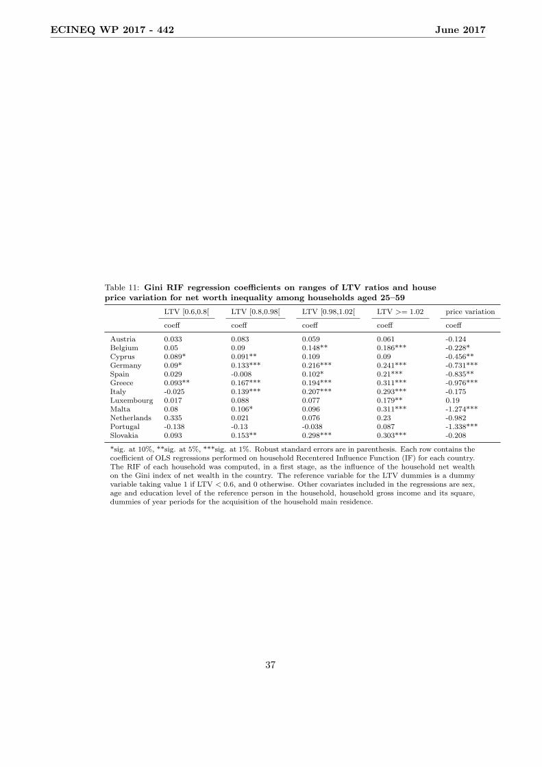
Table 11: Gini RIF regression coefficients on ranges of LTV ratios and houseprice variation for net worth inequality among households aged 25–59

LTV [0.6,0.8[ LTV [0.8,0.98[ LTV [0.98,1.02[ LTV >= 1.02 price variation


Austria 0.033 0.083 0.059 0.061 -0.124Belgium 0.05 0.09 0.148** 0.186*** -0.228*Cyprus 0.089* 0.091** 0.109 0.09 -0.456**Germany 0.09* 0.133*** 0.216*** 0.241*** -0.731***Spain 0.029 -0.008 0.102* 0.21*** -0.835**Greece 0.093** 0.167*** 0.194*** 0.311*** -0.976***Italy -0.025 0.139*** 0.207*** 0.293*** -0.175Luxembourg 0.017 0.088 0.077 0.179** 0.19Malta 0.08 0.106* 0.096 0.311*** -1.274***Netherlands 0.335 0.021 0.076 0.23 -0.982Portugal -0.138 -0.13 -0.038 0.087 -1.338***Slovakia 0.093 0.153** 0.298*** 0.303*** -0.208


37


(a) Effects on inequality by LTV ratio and mortgage cost.All the combinations of LTV ratios and mortgage falling onthe darker (lighter) area indicate a negative (positive) effectof LTV ratio on inequality (with β=0.90; γ=0.90)

(b) Effects on inequality by LTV ratio and bequest motive.All the combinations of LTV ratios and the strength of thebequest motive falling on the darker (lighter) area indicatea negative (positive) effect of LTV ratio on inequality (withβ=0.90; r=0.70)

Figure 1: Effects of LTV ratio changes (θ) on within inequality (Iw)

38


Fig

ure

2:

Influen

cefu

nct

ion

for

the

net

wort

hG

ini

coeffi

cien

tfo

rG

erm

any,

house

hold

saged

25–59

39


macroprudential policy and household wealth inequality · macroprudential policy and household...

Documents