foundations of modern macroeconomics - chapter …foundations of modern macroeconomics: chapter 11 2...
TRANSCRIPT

Foundations of Modern Macroeconomics: Chapter 11 1
Foundations of Modern MacroeconomicsB. J. Heijdra & F. van der Ploeg
Chapter 11: The Open Economy
Foundations of Modern Macroeconomics – Chapter 11 Version 1.06 – January 2005Ben J. Heijdra

Foundations of Modern Macroeconomics: Chapter 11 2
Aims of this lecture
• opening up the IS-LM model (sequel to material from Chapter 1): Mundell-Fleming
• fiscal and monetary policy in the open economy
– degree of capital mobility
– exchange rate system (fixed, flexible, managed)
• two-country IS-LM-AS models
– shock transmission
– international policy coordination
• open economy perfect foresight models (sequel to Chapter 4 material)
– role of price stickiness
– degree of capital mobility
– monetary accommodation
Foundations of Modern Macroeconomics – Chapter 11 Version 1.06 – January 2005Ben J. Heijdra
Foundations of Modern Macroeconomics: Chapter 11 3
National Income and Monetary Accounting
• For the open economy we have from the national accounts:
Y ≡ C + I + G + (EX − IM ) (A)
– Y is aggregate output
– C is private consumption
– I is investment
– G is government consumption
– EX is exports (demand by RoW for our products)
– IM is imports (demand by us for RoW’s products)
• We often write:
Y ≡ A + (EX − IM )
– A is absorption; EX − IM is net exportsFoundations of Modern Macroeconomics – Chapter 11 Version 1.06 – January 2005
Ben J. Heijdra

Foundations of Modern Macroeconomics: Chapter 11 4
• Remember output measurement:
– Gross Domestic Product (GDP): output produced within the country (“produced
where”)
– Gross National Product (GNP): output produced by the country’s residents
domestic (“produced by whom?”)
– difference: net factor payments from abroad
• We can add transfers (TR) and deduct taxes (T ) from (A) to get:
Y + TR − T︸ ︷︷ ︸(a)
≡ C + I + (G − T ) + (EX + TR − IM︸ ︷︷ ︸(b)
) (B)
– item (a): disposable income of residents
– item (b): current account CA (of the BoP)
Foundations of Modern Macroeconomics – Chapter 11 Version 1.06 – January 2005Ben J. Heijdra
Foundations of Modern Macroeconomics: Chapter 11 5
• Private sector saving:
S ≡ Y + TR − T − C (C)
• Combining (B) and (C):
(S − I) + (T − G) ≡ (EX + TR − IM ) ≡ CA
– current account surplus is sum of saving surpluses of private and public sectors
– CA measures additions to net external assets (CA > 0 means that domestic
country is lending to RoW):
∆NFA ≡ CA
≡ (S − I) + (T − G)
Foundations of Modern Macroeconomics – Chapter 11 Version 1.06 – January 2005Ben J. Heijdra

Foundations of Modern Macroeconomics: Chapter 11 6
• Now some monetary accounting: how does ∆NFA affect the monetary side of the
economy?
– look at ∆NFAcb (cb stands for Central Bank)
– stylized balance sheet:
Balance Sheet of the Central Bank
Assets Liabilities
Net foreign assets NFAcb
Domestic credit DC High powered money H
——– ——
Foundations of Modern Macroeconomics – Chapter 11 Version 1.06 – January 2005Ben J. Heijdra
Foundations of Modern Macroeconomics: Chapter 11 7
– NFAcb: foreign exchange reserves less liabilities to foreign official holders
– DC : securities held by CB (e.g. government bonds), loans, other credit
– H : stock of high-powered money (“base money”):
H ≡ CP + RE
where CP is currency and RE is commercial bank deposits held at CB
– by definition we get in first differences:
∆NFAcb ≡ ∆H − ∆DC (D)
Foundations of Modern Macroeconomics – Chapter 11 Version 1.06 – January 2005Ben J. Heijdra
Foundations of Modern Macroeconomics: Chapter 11 8
• Expression (D) yields important insights:
– if CB intervenes in foreign exchange market then, barring changes in DC , this
will affect (base) money supply: ∆NFAcb ≡ ∆H
– but CB can break link between NFAcb and H temporarily by sterilization:
manipulate DC to keep base money supply unchanged (∆NFAcb ≡ −∆DC
so that ∆H = 0). Example : sale of forex by CB =⇒ ∆NFAcb < 0,
expansionary open market operation (purchase of domestic bonds) =⇒
∆DC > 0.
• Final remark: in fractional reserve system we have that money supply is proportional
to base money, i.e. MS = µH and thus ∆MS = µ∆H .
Foundations of Modern Macroeconomics – Chapter 11 Version 1.06 – January 2005Ben J. Heijdra

Foundations of Modern Macroeconomics: Chapter 11 9
Open Economy IS-LM Model
• The IS curve for the open economy can be written as follows:
Y = A(r−, Y
+) + G + X(Y
−, Q
+),
Q ≡EP ∗
P
– A (r, Y ) is part of domestic absorption depending on r and Y ; partial
derivatives Ar < 0 (investment) and 0 < AY < 1 (MPC)
– X (Y,Q) is net exports; partial derivatives XY < 0 (import demand) and
XQ > 0 (Marshall-Lerner condition)
– Q is the relative price of foreign goods:
∗ E is nominal exchange rate (dimension Euro/US$)
∗ P is domestic price level (dimension Euro’s)
∗ P ∗ is foreign price level (dimension US$)
Foundations of Modern Macroeconomics – Chapter 11 Version 1.06 – January 2005Ben J. Heijdra
Foundations of Modern Macroeconomics: Chapter 11 10
• The LM curve for the open economy is represented by:
MD/P = L(r−, Y
+)
MS = µ[NFA
cb + DC]
MD = MS = M
• “Supply side.” Horizontal aggregate supply curves:
P = P ∗ = 1
Foundations of Modern Macroeconomics – Chapter 11 Version 1.06 – January 2005Ben J. Heijdra
Foundations of Modern Macroeconomics: Chapter 11 11
Capital Mobility and Economic Policy
• Alternative assumptions regarding “financial openness” of an economy:
– capital immobility: no trade in financial assets at all (1940s, early 1950s)
– perfect capital mobility: no barriers; equalization of yields (1980s onward)
– imperfect capital mobility: intermediate case
• Balance of payments:
B ≡ X(Y,Q) + KI (r − r∗) ≡ ∆NFAcb
– B is Balance of Payments
– X is trade account (ignoring international transfers, TR)
– KI is net capital inflow: if KI > 0 then domestic agents sell more assets to
RoW than RoW is buying from us; net borrowing from RoW.
– r∗ is interest rate in RoW
Foundations of Modern Macroeconomics – Chapter 11 Version 1.06 – January 2005Ben J. Heijdra
Foundations of Modern Macroeconomics: Chapter 11 12
• Cases mentioned above:
– capital immobility:
∗ KI (r − r∗) ≡ 0 regardless of r and r∗
∗ BoP equilibrium (B = 0) identical to trade balance equilibrium (X(Y,Q) = 0)
– perfect capital mobility:
∗ arbitrage ensures that r = r∗ (represented by KI r → +∞)
– imperfect capital mobility:
∗ differences in r and r∗ can persist (represented by 0 < KI r ≪ +∞)
– Note: in latter two cases, BoP equilibrium is such that X(Y,Q) = −KI (r− r∗)
• Three cases are drawn in Figure 11.1 .
Foundations of Modern Macroeconomics – Chapter 11 Version 1.06 – January 2005Ben J. Heijdra
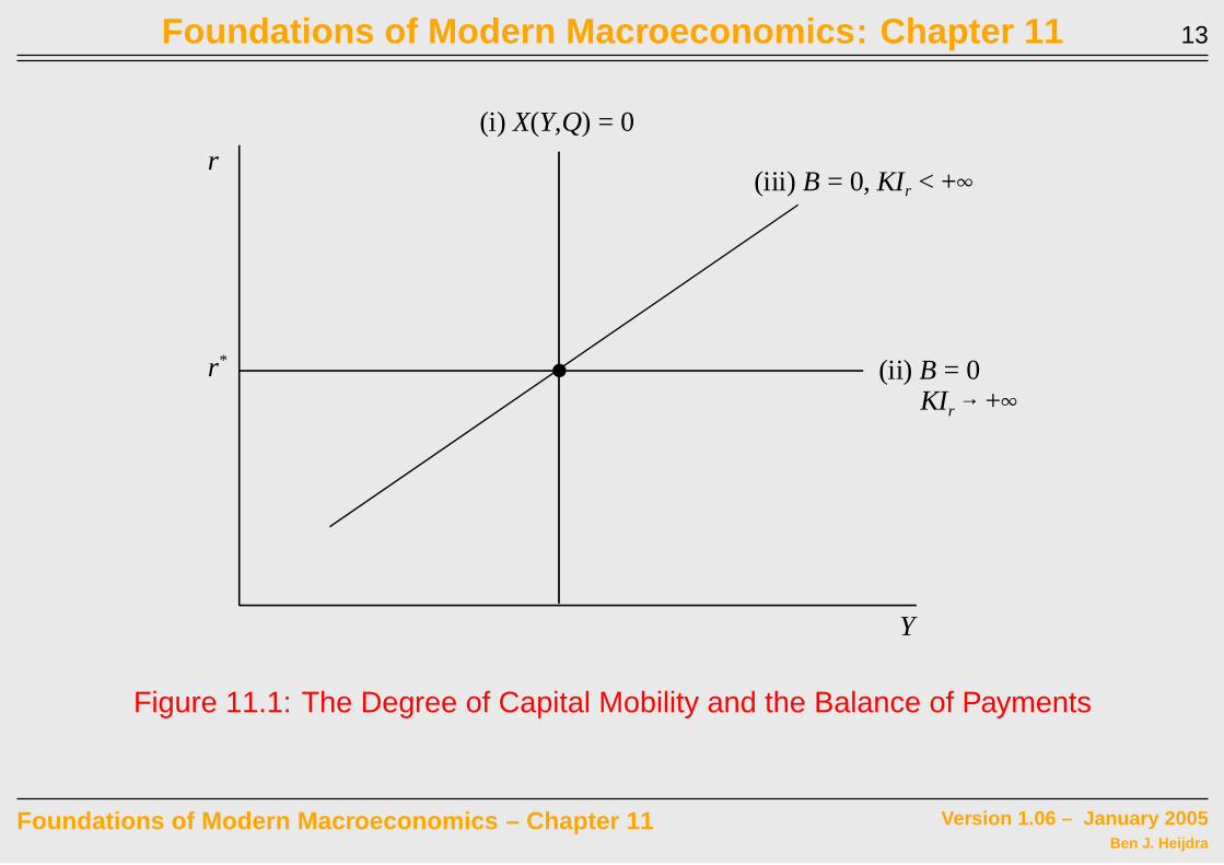
Foundations of Modern Macroeconomics: Chapter 11 13
r
Y
(iii) B = 0, KIr < +4
(i) X(Y,Q) = 0
(ii) B = 0r*!
KIr 6 +4
Figure 11.1: The Degree of Capital Mobility and the Balance of Payments
Foundations of Modern Macroeconomics – Chapter 11 Version 1.06 – January 2005Ben J. Heijdra

Foundations of Modern Macroeconomics: Chapter 11 14
Immobile Capital and Fixed Exchange Rates
• Assumptions:
– capital immobile: KI (r − r∗) ≡ 0
– monetary authority maintains exchange rate at E0
• Case is drawn in Figure 11.2 .
– IS downward sloping, LM upward sloping, X (Y,E0) = 0 line vertical
– to right (left) of X (Y,E0) = 0 imports too high (low) and B = X < 0 (> 0)
– initial equilibrium at point e0
Foundations of Modern Macroeconomics – Chapter 11 Version 1.06 – January 2005Ben J. Heijdra

Foundations of Modern Macroeconomics: Chapter 11 15
r
Y
X(Y,E0) = 0
X > 0 X < 0
Y0
r0
!
!
!
!
LM(M1)
LM(M0)
LM(M2)
IS(G0)
IS(G1)
YF
e0
e1
eN
eO
!
r1
Figure 11.2: Monetary and Fiscal Policy with Immobile Capital and Fixed Exchange Rates
Foundations of Modern Macroeconomics – Chapter 11 Version 1.06 – January 2005Ben J. Heijdra

Foundations of Modern Macroeconomics: Chapter 11 16
• Monetary policy:
– open market operation: purchase of bonds by CB, ∆DC > 0
– money supply goes up (from M0 to M1)
– LM to the right; economy to point e′
– at e′ there is excess demand for forex
– to keep exchange rate constant, CB must intervene (sell forex)
– money supply gradually falls; LM shifts to left
– economy back to e0
– Conclusion: no long-run effect on r and Y
Foundations of Modern Macroeconomics – Chapter 11 Version 1.06 – January 2005Ben J. Heijdra

Foundations of Modern Macroeconomics: Chapter 11 17
• Fiscal policy:
– bond financed increase in government consumption
– IS to the right; economy to point e′′
– at e′′ there is excess demand for forex
– to keep exchange rate constant, CB must intervene (sell forex)
– money supply gradually falls; LM shifts to left
– economy moves to e1
– Conclusion: no long-run effect on Y but r higher
– crowding out of investment
Foundations of Modern Macroeconomics – Chapter 11 Version 1.06 – January 2005Ben J. Heijdra

Foundations of Modern Macroeconomics: Chapter 11 18
Perfectly Mobile Capital and Fixed Exchange Rates
• Assumptions:
– capital perfectly mobile: r = r∗
– monetary authority maintains exchange rate at E0
– BP curve is horizontal in Figure 11.3
– economy initially at e0
• Monetary policy:
– OMO increases DC and money supply; LM to right
– at e′ excess demand for forex (investors want to buy foreign assets)
– CB intervenes and loses its foreign reserves; LM back
– adjustment is instantaneous, so monetary policy ineffective even in short run
Foundations of Modern Macroeconomics – Chapter 11 Version 1.06 – January 2005Ben J. Heijdra

Foundations of Modern Macroeconomics: Chapter 11 19
• Fiscal policy:
– bond financed increase in government consumption
– IS to the right; economy to point e′′
– at e′′ there is excess supply of forex (investors dump foreign assets)
– to keep exchange rate constant, CB must intervene (buy forex)
– money supply increases; LM to the right, economy moves to e1
– adjustment is instantaneous: no effect on r but Y higher
– fiscal policy highly effective
Foundations of Modern Macroeconomics – Chapter 11 Version 1.06 – January 2005Ben J. Heijdra

Foundations of Modern Macroeconomics: Chapter 11 20
r
YY0
r*
!
!
!
!
LM(M1)
LM(M0)
IS(G0)
IS(G1)
Y1
e0e1
eN
eO
Figure 11.3: Monetary and Fiscal Policy with PCM and Fixed Exchange Rates
Foundations of Modern Macroeconomics – Chapter 11 Version 1.06 – January 2005Ben J. Heijdra

Foundations of Modern Macroeconomics: Chapter 11 21
Perfect Capital Mobility and Flexible Exchange Rates
• the flexible exchange rate ensures BoP equilibrium:
B ≡ ∆NFAcb = 0 ⇔
X(Y,E) + KI (r − r∗) = 0
– imports: cause demand for forex
– exports: cause supply of forex
– capital imports: cause supply of forex
– Recall: no exchange rate intervention by CB, so stock of forex in hands of CB
constant. Change in DC affects money supply. Money supply can be controlled.
• focus on case with perfect capital mobility (PCM)
Foundations of Modern Macroeconomics – Chapter 11 Version 1.06 – January 2005Ben J. Heijdra
Foundations of Modern Macroeconomics: Chapter 11 22
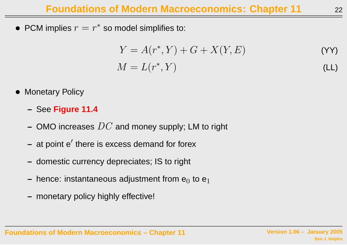
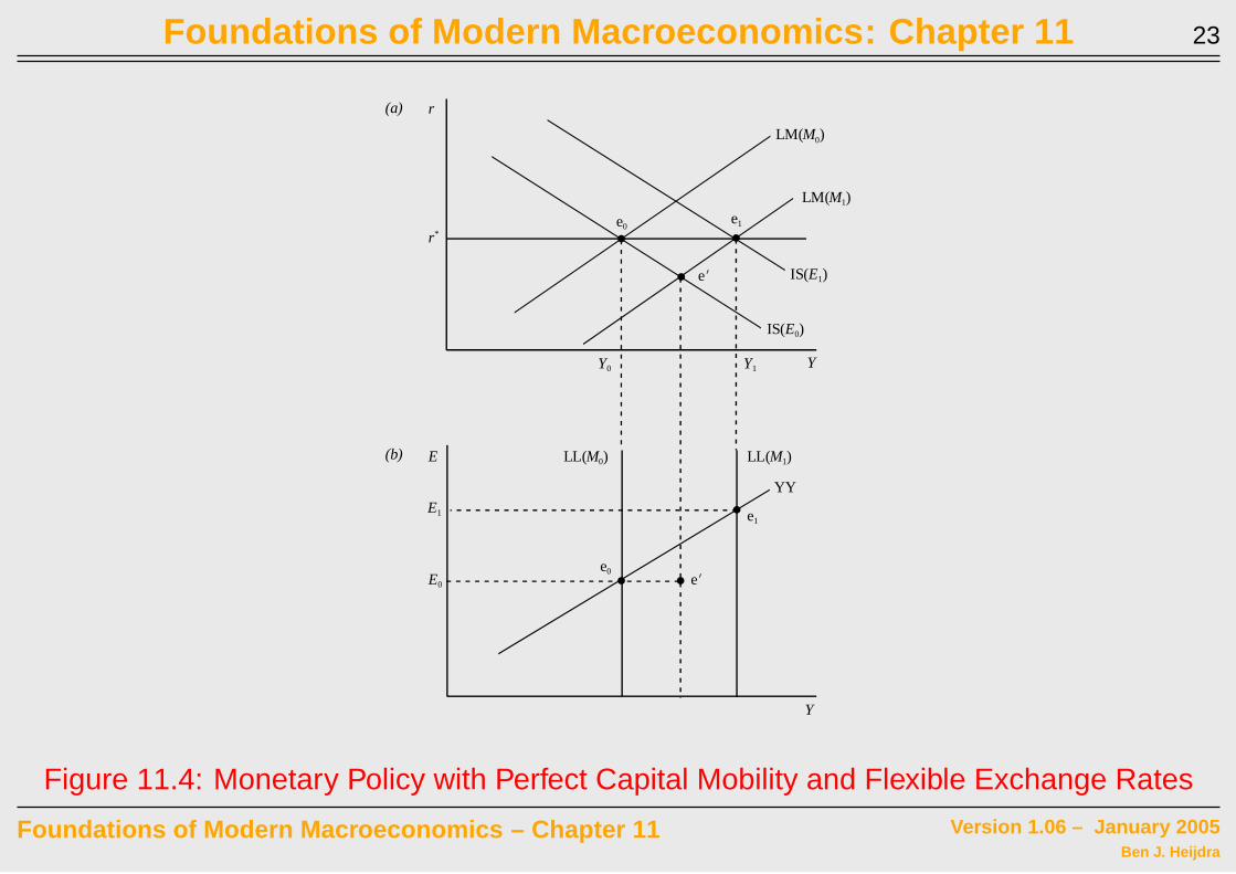
• PCM implies r = r∗ so model simplifies to:
Y = A(r∗, Y ) + G + X(Y,E) (YY)
M = L(r∗, Y ) (LL)
• Monetary Policy
– See Figure 11.4
– OMO increases DC and money supply; LM to right
– at point e′ there is excess demand for forex
– domestic currency depreciates; IS to right
– hence: instantaneous adjustment from e0 to e1
– monetary policy highly effective!
Foundations of Modern Macroeconomics – Chapter 11 Version 1.06 – January 2005Ben J. Heijdra
Foundations of Modern Macroeconomics: Chapter 11 23
r
YY0
r*!
!
!
LM(M1)
LM(M0)
IS(E0)
IS(E1)
Y1
e0e1
eN
e0
e1
eN!
!
!
YY
LL(M0) LL(M1)
E0
E1
E
Y
(a)
(b)
Figure 11.4: Monetary Policy with Perfect Capital Mobility and Flexible Exchange Rates
Foundations of Modern Macroeconomics – Chapter 11 Version 1.06 – January 2005Ben J. Heijdra

Foundations of Modern Macroeconomics: Chapter 11 24
• Fiscal Policy
– See Figure 11.5
– bond financed increase in government consumption; IS to right
– at point e′ there is excess supply of forex
– domestic currency appreciates; IS to left
– hence: economy stays at e0
– fiscal policy completely ineffective!
Foundations of Modern Macroeconomics – Chapter 11 Version 1.06 – January 2005Ben J. Heijdra

Foundations of Modern Macroeconomics: Chapter 11 25
r
YY0
r*
!
!
LM
IS(G1,E0)
e0
eN
e0
e1
eN!
!
!
LL
YY(G0)
E0
E1
E
Y
IS(G0,E0)
IS(G1,E1)
YY(G1)
(a)
(b)
Figure 11.5: Fiscal Policy with Perfect Capital Mobility and Flexible Exchange Rates
Foundations of Modern Macroeconomics – Chapter 11 Version 1.06 – January 2005Ben J. Heijdra

Foundations of Modern Macroeconomics: Chapter 11 26
• Insulation Property
– flexible exchange rates insulate small open economy from foreign shocks
(provided r∗ is unaffected).
– Example: RoW spending boom. Our exports rise, YY curve to the right, exchange
rate appreciates, no effect on output. Shock not transmitted to quantities.
• For global shocks no insulation property:
– Example: boost in RoW driving up world interest rate, r∗
– See Figure 11.6
– LL to right; YY up; domestic currency appreciates; output increases
Foundations of Modern Macroeconomics – Chapter 11 Version 1.06 – January 2005Ben J. Heijdra

Foundations of Modern Macroeconomics: Chapter 11 27
r
YY0
r0
!
!
LM
IS(E1)
Y1
e0
e0
e1
!
!
YY(r0)
E0
E1
E
Y
IS(E0)
YY(r1)
e1
r1
LL(r1)LL(r0)
(a)
(b)
Figure 11.6: World Interest Rate Shock with PCM and Flexible Exchange Rates
Foundations of Modern Macroeconomics – Chapter 11 Version 1.06 – January 2005Ben J. Heijdra
Foundations of Modern Macroeconomics: Chapter 11 28
Summary on Open Economy IS-LM-BP Model
• exchange rate regime matters a lot
– completely fixed exchange rates
– completely flexible exchange rates
– intermediate case: managed float (see below)
• mobility of financial capital matters a lot
– no mobility
– perfect mobility
– intermediate case: imperfect capital mobility (see Figure 11.7 and Table 11.1 )
Foundations of Modern Macroeconomics – Chapter 11 Version 1.06 – January 2005Ben J. Heijdra

Foundations of Modern Macroeconomics: Chapter 11 29
r
YY0
r1 !
!
!
LM(M1)LM(M0)
IS(E0)
IS(E1)
Y1
e0
e1
eN
r0
BP(E0)
BP(E1)
Figure 11.7: Monetary Policy with Imperfect Capital Mobility and Flexible Exchange Rates
Foundations of Modern Macroeconomics – Chapter 11 Version 1.06 – January 2005Ben J. Heijdra
Foundations of Modern Macroeconomics: Chapter 11 30
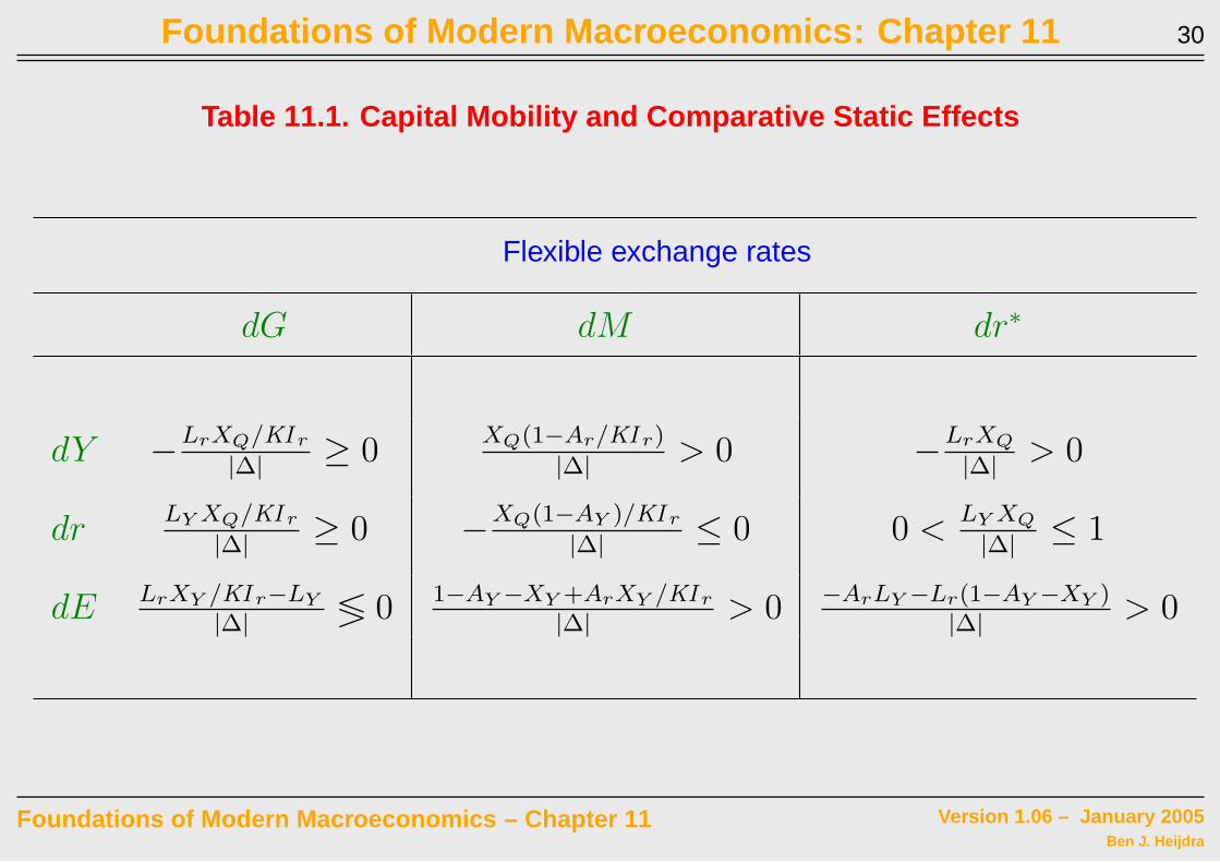
Table 11.1. Capital Mobility and Comparative Static Effects
Flexible exchange rates
dG dM dr∗
dY −LrXQ/KI r
|∆|≥ 0
XQ(1−Ar/KI r)
|∆|> 0 −
LrXQ
|∆|> 0
drLY XQ/KI r
|∆|≥ 0 −
XQ(1−AY )/KI r
|∆|≤ 0 0 <
LY XQ
|∆|≤ 1
dE LrXY /KI r−LY
|∆|≶ 0 1−AY −XY +ArXY /KI r
|∆|> 0 −ArLY −Lr(1−AY −XY )
|∆|> 0
Foundations of Modern Macroeconomics – Chapter 11 Version 1.06 – January 2005Ben J. Heijdra

Foundations of Modern Macroeconomics: Chapter 11 31
Table 11.1. Capital Mobility and Comparative Static Effects (continu ed)
Fixed exchange rates
dG dE dr∗
dY 1|Γ|
> 0XQ(1−Ar/KI r)
|Γ|> 0 Ar
|Γ|< 0
dr −XY /KI r
|Γ|≥ 0 −
(1−AY )XQ/KI r
|Γ|< 0 0 < 1−AY −XY
|Γ|≤ 1
dM LY −LrXY /KI r
|Γ|≷ 0 |∆|
|Γ|> 0 ArLY +Lr(1−AY −XY )
|Γ|< 0
Foundations of Modern Macroeconomics – Chapter 11 Version 1.06 – January 2005Ben J. Heijdra

Foundations of Modern Macroeconomics: Chapter 11 32
Supply Side
• assumed so far: horizontal AS curves in the domestic economy and in the RoW:
P = P ∗ = 1 (constant)
• adding the supply side important because:
– “microeconomic” foundation behind demand/supply curves
– consistent treatment of cost-of-living indexes
– used later to study international shock transmission
Foundations of Modern Macroeconomics – Chapter 11 Version 1.06 – January 2005Ben J. Heijdra
Foundations of Modern Macroeconomics: Chapter 11 33
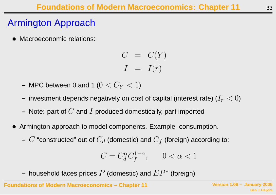
Armington Approach
• Macroeconomic relations:
C = C(Y )
I = I(r)
– MPC between 0 and 1 (0 < CY < 1)
– investment depends negatively on cost of capital (interest rate) (Ir < 0)
– Note: part of C and I produced domestically, part imported
• Armington approach to model components. Example consumption.
– C “constructed” out of Cd (domestic) and Cf (foreign) according to:
C = Cαd C1−α
f , 0 < α < 1
– household faces prices P (domestic) and EP ∗ (foreign)
Foundations of Modern Macroeconomics – Chapter 11 Version 1.06 – January 2005Ben J. Heijdra
Foundations of Modern Macroeconomics: Chapter 11 34
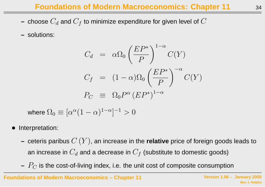
– choose Cd and Cf to minimize expenditure for given level of C
– solutions:
Cd = αΩ0
(EP ∗
P
)1−α
C(Y )
Cf = (1 − α)Ω0
(EP ∗
P
)−α
C(Y )
PC ≡ Ω0Pα (EP ∗)1−α
where Ω0 ≡ [αα(1 − α)1−α]−1 > 0
• Interpretation:
– ceteris paribus C (Y ), an increase in the relative price of foreign goods leads to
an increase in Cd and a decrease in Cf (substitute to domestic goods)
– PC is the cost-of-living index, i.e. the unit cost of composite consumption
Foundations of Modern Macroeconomics – Chapter 11 Version 1.06 – January 2005Ben J. Heijdra

Foundations of Modern Macroeconomics: Chapter 11 35
• We can use the same trick for investment and for government consumption:
– assume same α (as for C) for simplicity:
I = Iαd I1−α
f
G = GαdG1−α
f
– solutions:
Id = αΩ0
(EP ∗
P
)1−α
I(r)
If = (1 − α)Ω0
(EP ∗
P
)−α
I(r)
Gd = αΩ0
(EP ∗
P
)1−α
G
Gf = (1 − α)Ω0
(EP ∗
P
)−α
G
Foundations of Modern Macroeconomics – Chapter 11 Version 1.06 – January 2005Ben J. Heijdra
Foundations of Modern Macroeconomics: Chapter 11 36
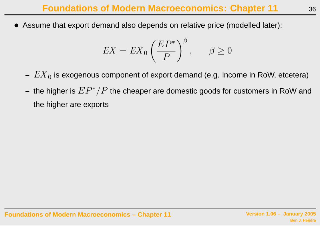
• Assume that export demand also depends on relative price (modelled later):
EX = EX 0
(EP ∗
P
)β
, β ≥ 0
– EX 0 is exogenous component of export demand (e.g. income in RoW, etcetera)
– the higher is EP ∗/P the cheaper are domestic goods for customers in RoW and
the higher are exports
Foundations of Modern Macroeconomics – Chapter 11 Version 1.06 – January 2005Ben J. Heijdra
Foundations of Modern Macroeconomics: Chapter 11 37
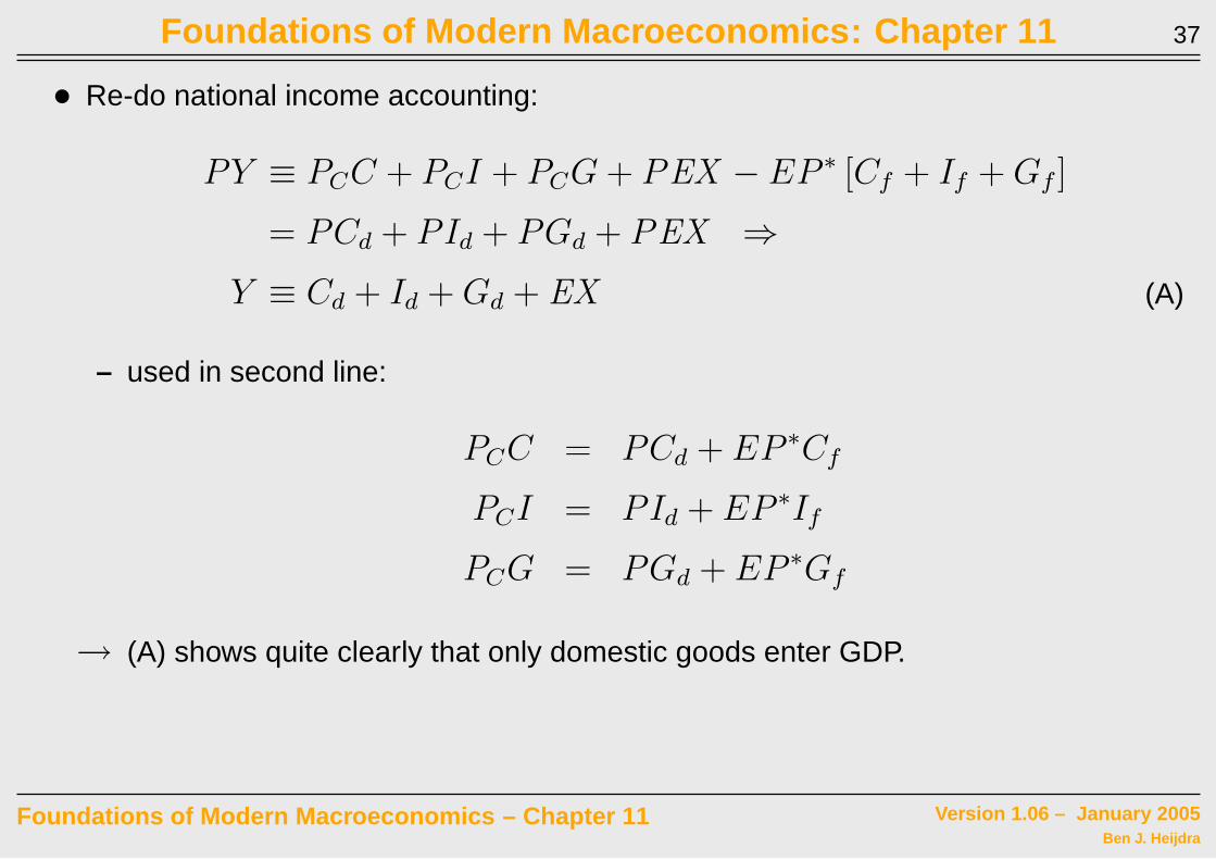
• Re-do national income accounting:
PY ≡ PCC + PCI + PCG + PEX − EP ∗ [Cf + If + Gf ]
= PCd + PId + PGd + PEX ⇒
Y ≡ Cd + Id + Gd + EX (A)
– used in second line:
PCC = PCd + EP ∗Cf
PCI = PId + EP ∗If
PCG = PGd + EP ∗Gf
→ (A) shows quite clearly that only domestic goods enter GDP.
Foundations of Modern Macroeconomics – Chapter 11 Version 1.06 – January 2005Ben J. Heijdra
Foundations of Modern Macroeconomics: Chapter 11 38
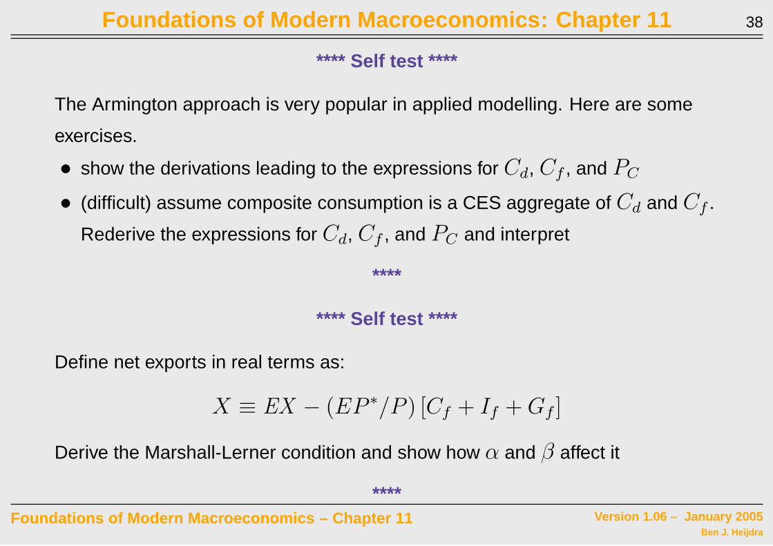
**** Self test ****
The Armington approach is very popular in applied modelling. Here are some
exercises.
• show the derivations leading to the expressions for Cd, Cf , and PC
• (difficult) assume composite consumption is a CES aggregate of Cd and Cf .
Rederive the expressions for Cd, Cf , and PC and interpret
****
**** Self test ****
Define net exports in real terms as:
X ≡ EX − (EP ∗/P ) [Cf + If + Gf ]
Derive the Marshall-Lerner condition and show how α and β affect it
****Foundations of Modern Macroeconomics – Chapter 11 Version 1.06 – January 2005
Ben J. Heijdra
Foundations of Modern Macroeconomics: Chapter 11 39
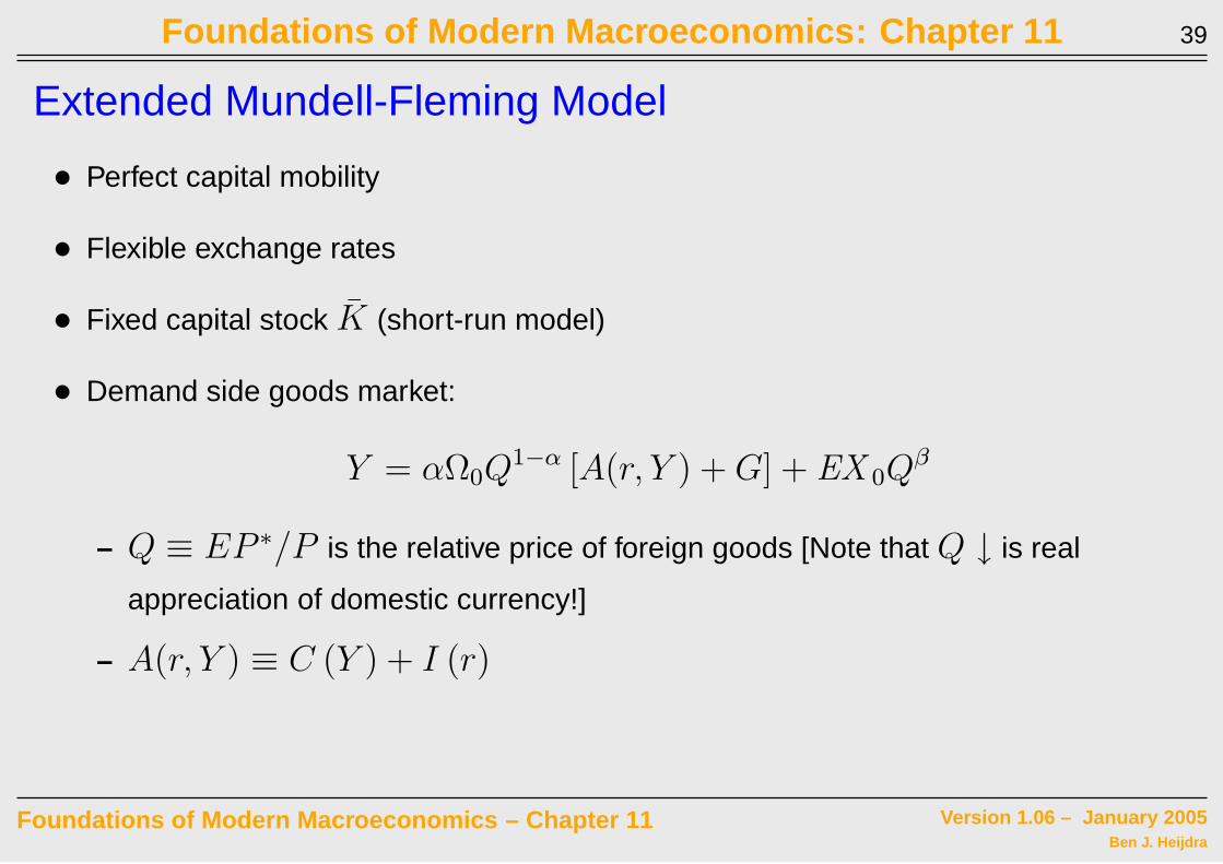
Extended Mundell-Fleming Model
• Perfect capital mobility
• Flexible exchange rates
• Fixed capital stock K (short-run model)
• Demand side goods market:
Y = αΩ0Q1−α [A(r, Y ) + G] + EX 0Q
β
– Q ≡ EP ∗/P is the relative price of foreign goods [Note that Q ↓ is real
appreciation of domestic currency!]
– A(r, Y ) ≡ C (Y ) + I (r)
Foundations of Modern Macroeconomics – Chapter 11 Version 1.06 – January 2005Ben J. Heijdra
Foundations of Modern Macroeconomics: Chapter 11 40
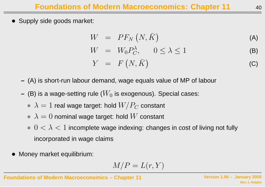
• Supply side goods market:
W = PFN
(N, K
)(A)
W = W0PλC , 0 ≤ λ ≤ 1 (B)
Y = F(N, K
)(C)
– (A) is short-run labour demand, wage equals value of MP of labour
– (B) is a wage-setting rule (W0 is exogenous). Special cases:
∗ λ = 1 real wage target: hold W/PC constant
∗ λ = 0 nominal wage target: hold W constant
∗ 0 < λ < 1 incomplete wage indexing: changes in cost of living not fully
incorporated in wage claims
• Money market equilibrium:
M/P = L(r, Y )
Foundations of Modern Macroeconomics – Chapter 11 Version 1.06 – January 2005Ben J. Heijdra

Foundations of Modern Macroeconomics: Chapter 11 41
• Perfect capital mobility:
r = r∗
• The model can be analyzed
– . . . mathematically by log-linearizing it—see Table 11.2 for the key expressions.
– . . . graphically by means of Figure 11.8 .
Foundations of Modern Macroeconomics – Chapter 11 Version 1.06 – January 2005Ben J. Heijdra
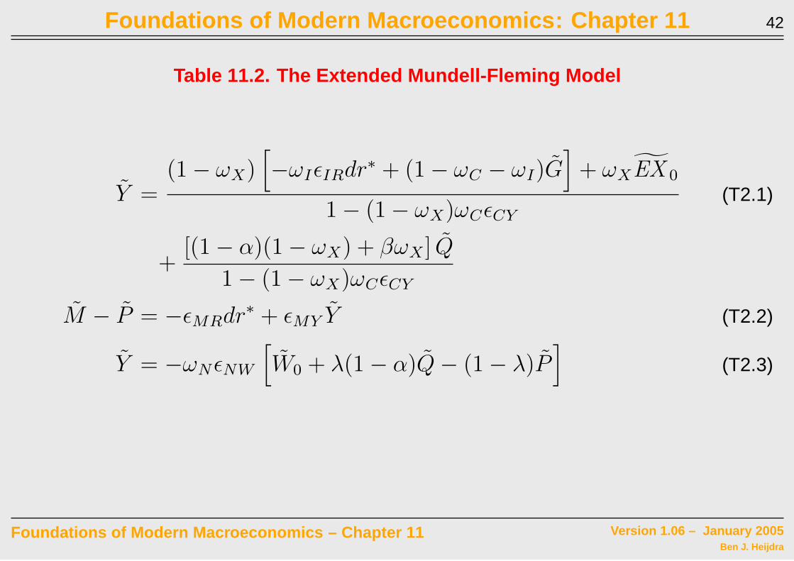
Foundations of Modern Macroeconomics: Chapter 11 42
Table 11.2. The Extended Mundell-Fleming Model
Y =(1 − ωX)
[−ωIǫIRdr∗ + (1 − ωC − ωI)G
]+ ωXEX 0
1 − (1 − ωX)ωCǫCY
(T2.1)
+[(1 − α)(1 − ωX) + βωX ] Q
1 − (1 − ωX)ωCǫCY
M − P = −ǫMRdr∗ + ǫMY Y (T2.2)
Y = −ωNǫNW
[W0 + λ(1 − α)Q − (1 − λ)P
](T2.3)
Foundations of Modern Macroeconomics – Chapter 11 Version 1.06 – January 2005Ben J. Heijdra
Foundations of Modern Macroeconomics: Chapter 11 43
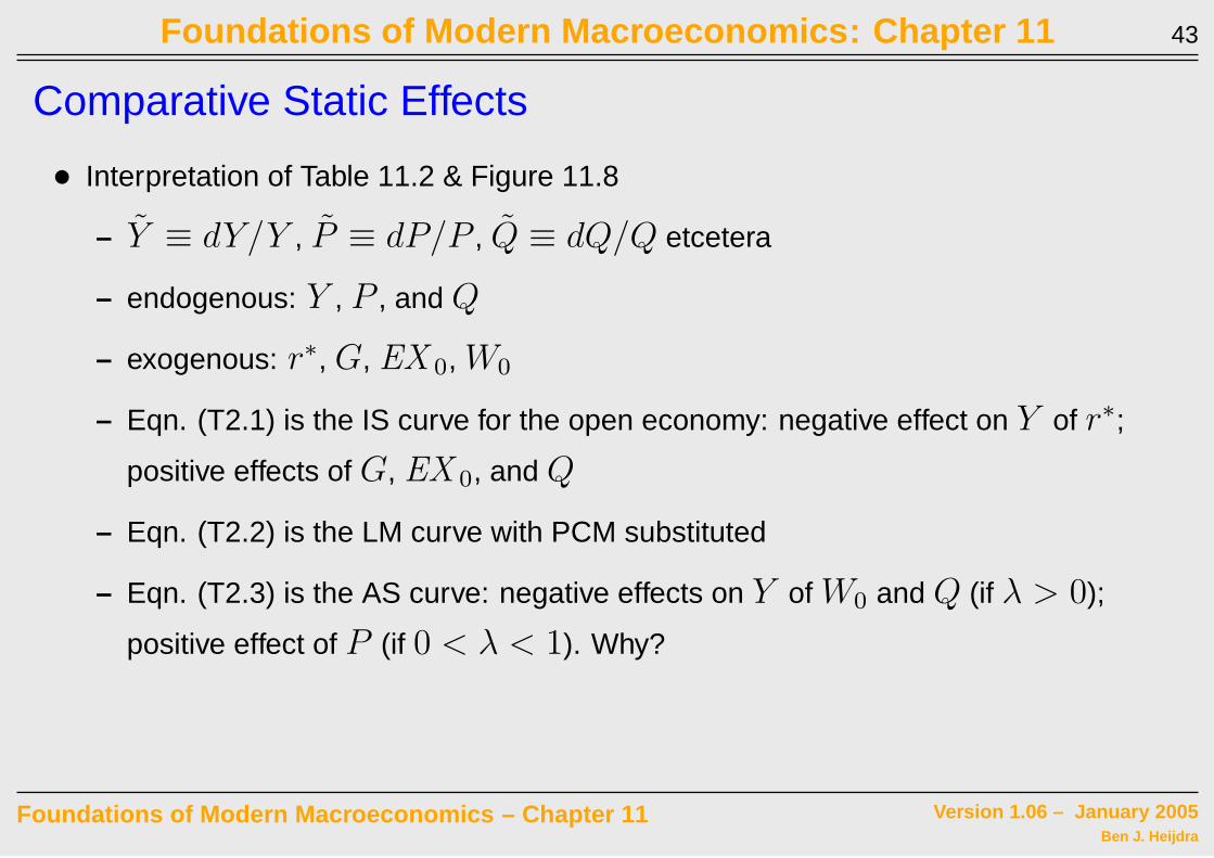
Comparative Static Effects
• Interpretation of Table 11.2 & Figure 11.8
– Y ≡ dY/Y , P ≡ dP/P , Q ≡ dQ/Q etcetera
– endogenous: Y , P , and Q
– exogenous: r∗, G, EX 0, W0
– Eqn. (T2.1) is the IS curve for the open economy: negative effect on Y of r∗;
positive effects of G, EX 0, and Q
– Eqn. (T2.2) is the LM curve with PCM substituted
– Eqn. (T2.3) is the AS curve: negative effects on Y of W0 and Q (if λ > 0);
positive effect of P (if 0 < λ < 1). Why?
Foundations of Modern Macroeconomics – Chapter 11 Version 1.06 – January 2005Ben J. Heijdra
Foundations of Modern Macroeconomics: Chapter 11 44
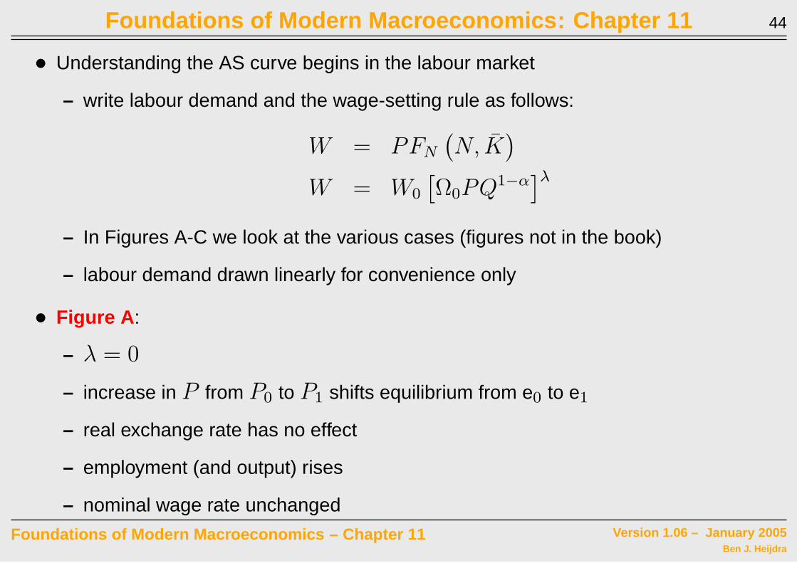
• Understanding the AS curve begins in the labour market
– write labour demand and the wage-setting rule as follows:
W = PFN
(N, K
)
W = W0
[Ω0PQ1−α
]λ
– In Figures A-C we look at the various cases (figures not in the book)
– labour demand drawn linearly for convenience only
• Figure A :
– λ = 0
– increase in P from P0 to P1 shifts equilibrium from e0 to e1
– real exchange rate has no effect
– employment (and output) rises
– nominal wage rate unchanged
Foundations of Modern Macroeconomics – Chapter 11 Version 1.06 – January 2005Ben J. Heijdra
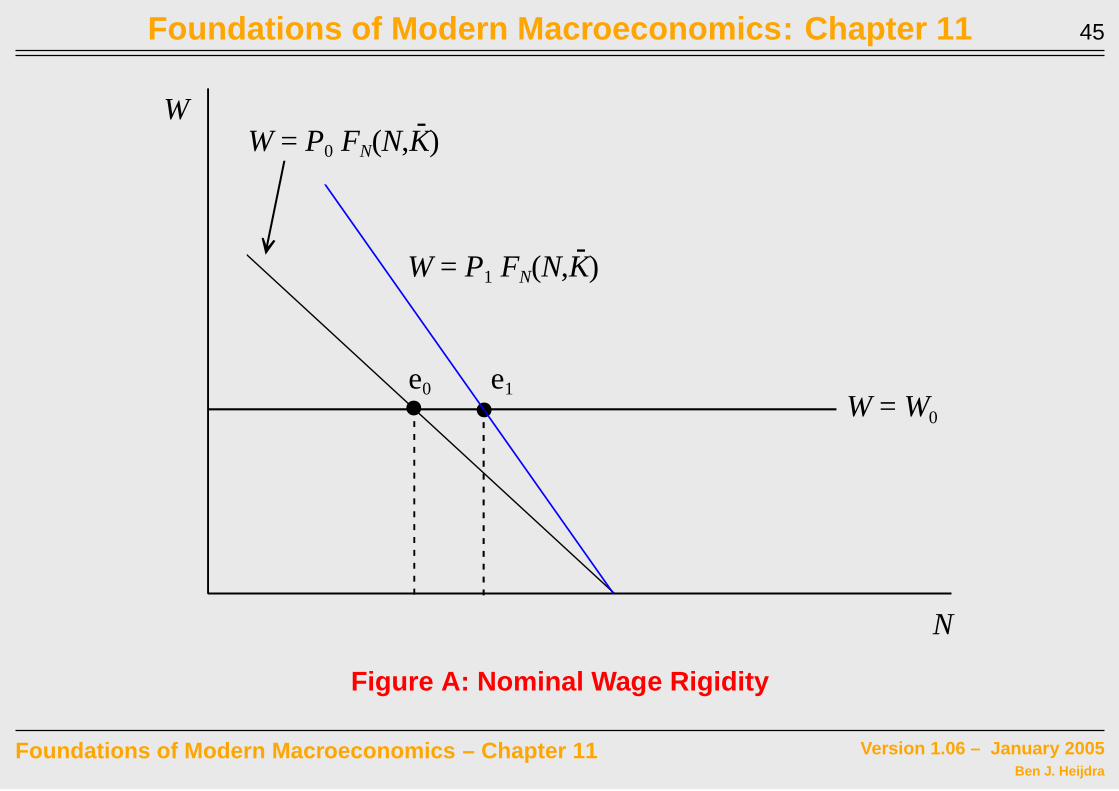
Foundations of Modern Macroeconomics: Chapter 11 45
W
N
! !
W = P0 FN(N,K)-
e0 e1
W = P1 FN(N,K)-
W = W0
Figure A: Nominal Wage Rigidity
Foundations of Modern Macroeconomics – Chapter 11 Version 1.06 – January 2005Ben J. Heijdra
Foundations of Modern Macroeconomics: Chapter 11 46
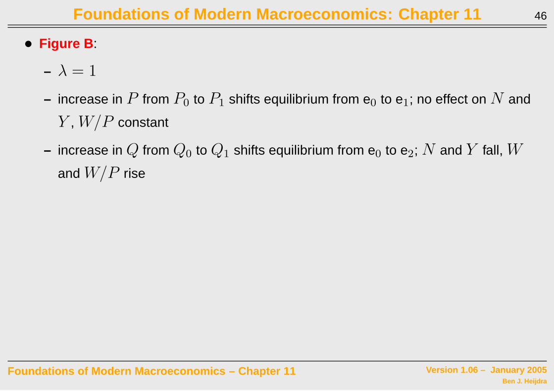
• Figure B :
– λ = 1
– increase in P from P0 to P1 shifts equilibrium from e0 to e1; no effect on N and
Y , W/P constant
– increase in Q from Q0 to Q1 shifts equilibrium from e0 to e2; N and Y fall, W
and W/P rise
Foundations of Modern Macroeconomics – Chapter 11 Version 1.06 – January 2005Ben J. Heijdra

Foundations of Modern Macroeconomics: Chapter 11 47
W
N
!
!
W = P0 FN(N,K)-
e0
e1
W = P1 FN(N,K)-
W = W0 S0 P1 Q1-"0
W = W0 S0 P0 Q1-"0
W = W0 S0 P1 Q1-"1e2
!
Figure B: Real Wage Rigidity
Foundations of Modern Macroeconomics – Chapter 11 Version 1.06 – January 2005Ben J. Heijdra
Foundations of Modern Macroeconomics: Chapter 11 48
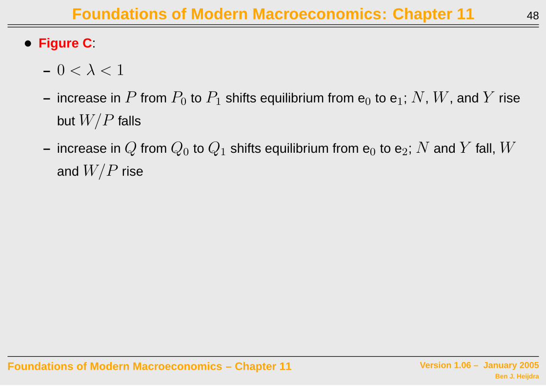
• Figure C :
– 0 < λ < 1
– increase in P from P0 to P1 shifts equilibrium from e0 to e1; N , W , and Y rise
but W/P falls
– increase in Q from Q0 to Q1 shifts equilibrium from e0 to e2; N and Y fall, W
and W/P rise
Foundations of Modern Macroeconomics – Chapter 11 Version 1.06 – January 2005Ben J. Heijdra

Foundations of Modern Macroeconomics: Chapter 11 49
W
N
!
!
W = P0 FN(N,K)-
e0
e1
W = P1 FN(N,K)-
W = W0 S0 P1 Q8(1-")0
8 8 8
e2
!
W = W0 S0 P0 Q8(1-")1
8 8 8
W = W0 S0 P0 Q8(1-")0
8 8 8
Figure C: Incomplete Wage Indexing
Foundations of Modern Macroeconomics – Chapter 11 Version 1.06 – January 2005Ben J. Heijdra

Foundations of Modern Macroeconomics: Chapter 11 50
P
Y0
Q1
!
! !
LMAS(LM)
IS(G1)
IS(G0)Y1
e0
e1
Q0
Y
Q
AS(LM)(8 = 0)
(8 > 0)
Q2P1P0
!
!
e2e0
e1
Figure 11.8: Aggregate Demand Shocks under Wage Rigidity
Foundations of Modern Macroeconomics – Chapter 11 Version 1.06 – January 2005Ben J. Heijdra
Foundations of Modern Macroeconomics: Chapter 11 51
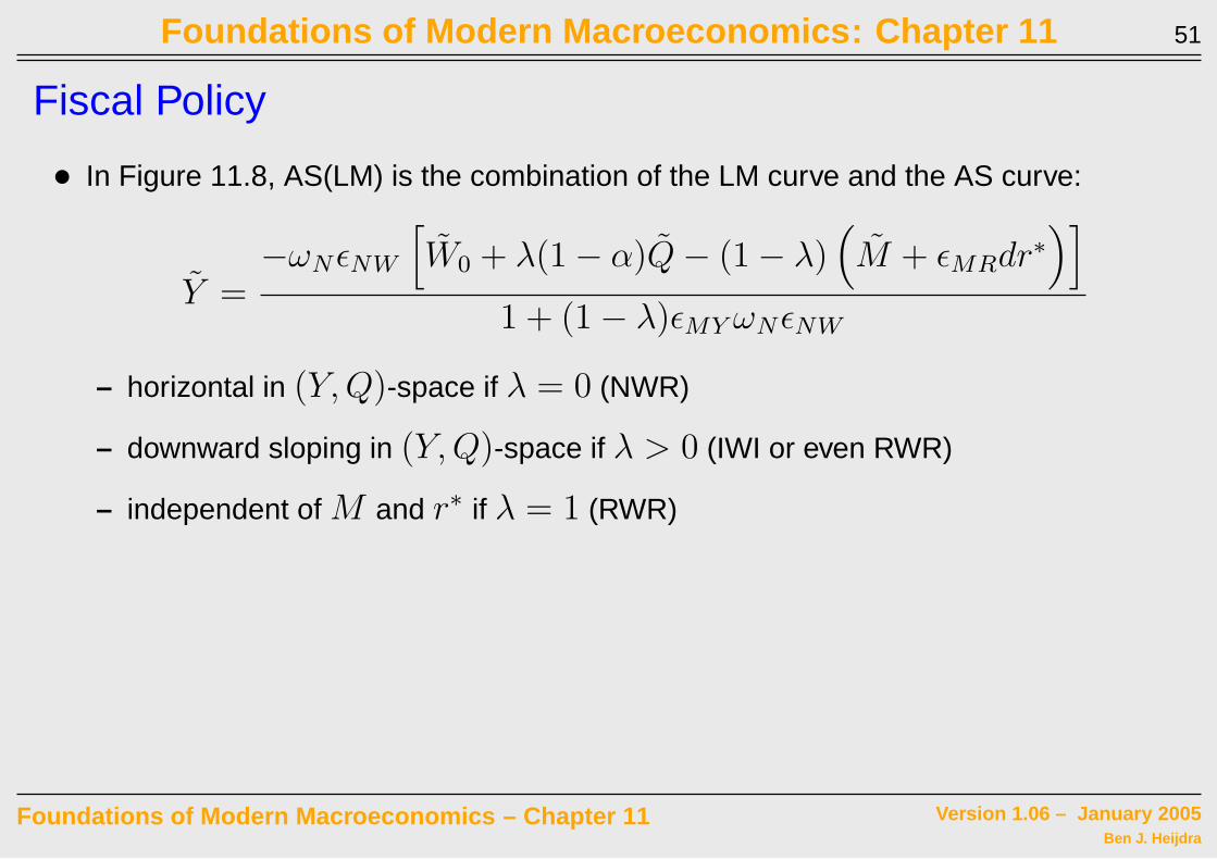
Fiscal Policy
• In Figure 11.8, AS(LM) is the combination of the LM curve and the AS curve:
Y =−ωNǫNW
[W0 + λ(1 − α)Q − (1 − λ)
(M + ǫMRdr∗
)]
1 + (1 − λ)ǫMY ωNǫNW
– horizontal in (Y,Q)-space if λ = 0 (NWR)
– downward sloping in (Y,Q)-space if λ > 0 (IWI or even RWR)
– independent of M and r∗ if λ = 1 (RWR)
Foundations of Modern Macroeconomics – Chapter 11 Version 1.06 – January 2005Ben J. Heijdra
Foundations of Modern Macroeconomics: Chapter 11 52
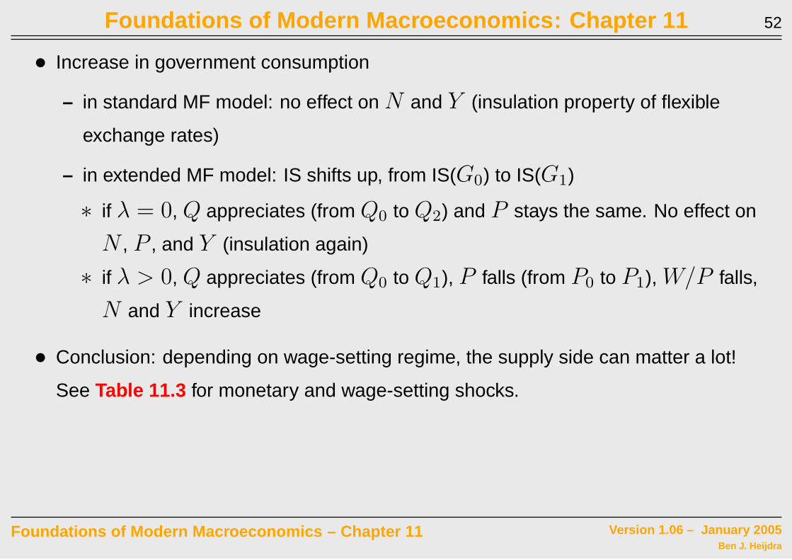
• Increase in government consumption
– in standard MF model: no effect on N and Y (insulation property of flexible
exchange rates)
– in extended MF model: IS shifts up, from IS(G0) to IS(G1)
∗ if λ = 0, Q appreciates (from Q0 to Q2) and P stays the same. No effect on
N , P , and Y (insulation again)
∗ if λ > 0, Q appreciates (from Q0 to Q1), P falls (from P0 to P1), W/P falls,
N and Y increase
• Conclusion: depending on wage-setting regime, the supply side can matter a lot!
See Table 11.3 for monetary and wage-setting shocks.
Foundations of Modern Macroeconomics – Chapter 11 Version 1.06 – January 2005Ben J. Heijdra
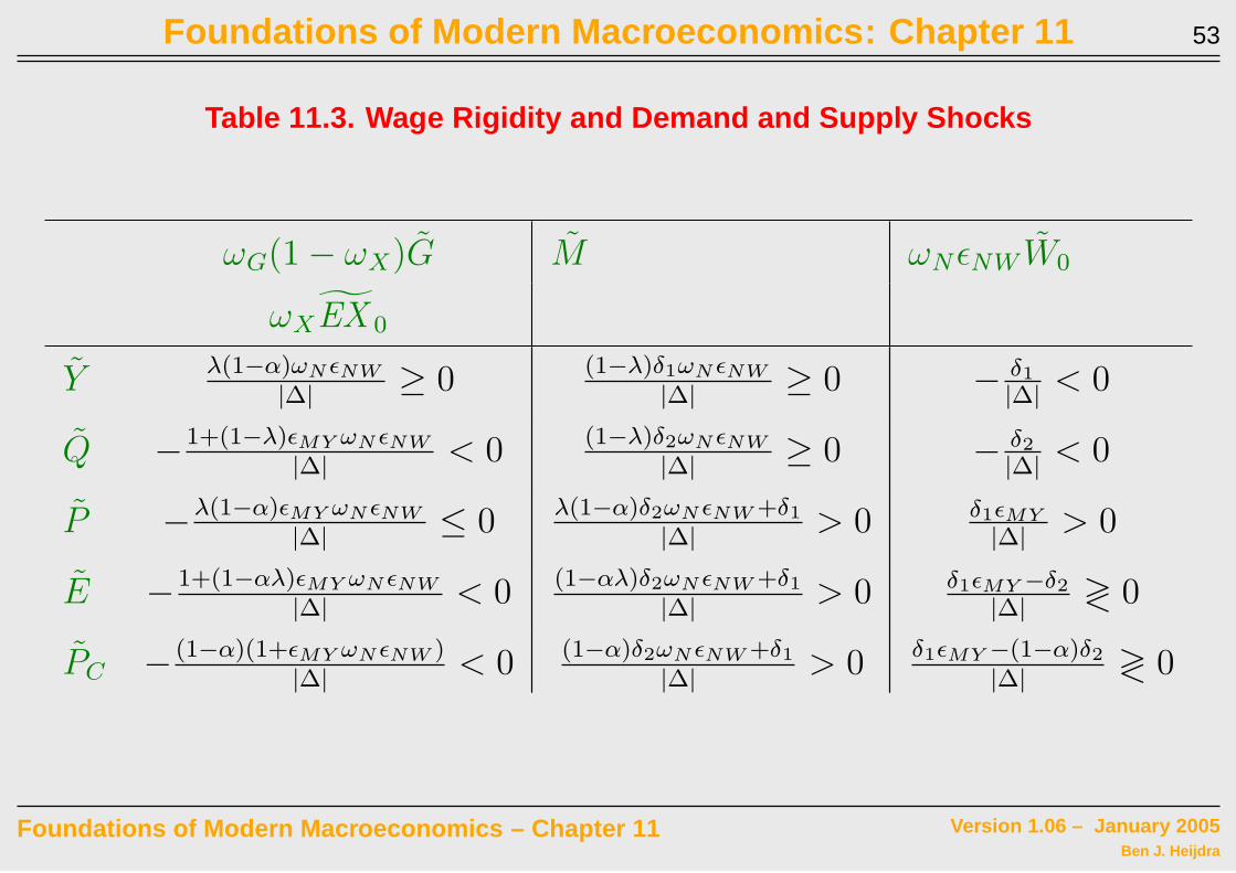
Foundations of Modern Macroeconomics: Chapter 11 53
Table 11.3. Wage Rigidity and Demand and Supply Shocks
ωG(1 − ωX)G M ωNǫNW W0
ωXEX 0
Y λ(1−α)ωN ǫNW
|∆|≥ 0 (1−λ)δ1ωN ǫNW
|∆|≥ 0 − δ1
|∆|< 0
Q −1+(1−λ)ǫMY ωN ǫNW
|∆|< 0 (1−λ)δ2ωN ǫNW
|∆|≥ 0 − δ2
|∆|< 0
P −λ(1−α)ǫMY ωN ǫNW
|∆|≤ 0 λ(1−α)δ2ωN ǫNW +δ1
|∆|> 0 δ1ǫMY
|∆|> 0
E −1+(1−αλ)ǫMY ωN ǫNW
|∆|< 0 (1−αλ)δ2ωN ǫNW +δ1
|∆|> 0 δ1ǫMY −δ2
|∆|≷ 0
PC −(1−α)(1+ǫMY ωN ǫNW )
|∆|< 0 (1−α)δ2ωN ǫNW +δ1
|∆|> 0 δ1ǫMY −(1−α)δ2
|∆|≷ 0
Foundations of Modern Macroeconomics – Chapter 11 Version 1.06 – January 2005Ben J. Heijdra
Foundations of Modern Macroeconomics: Chapter 11 54
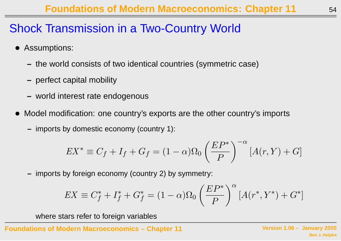
Shock Transmission in a Two-Country World
• Assumptions:
– the world consists of two identical countries (symmetric case)
– perfect capital mobility
– world interest rate endogenous
• Model modification: one country’s exports are the other country’s imports
– imports by domestic economy (country 1):
EX∗ ≡ Cf + If + Gf = (1 − α)Ω0
(EP ∗
P
)−α
[A(r, Y ) + G]
– imports by foreign economy (country 2) by symmetry:
EX ≡ C∗f + I∗f + G∗
f = (1 − α)Ω0
(EP ∗
P
)α
[A(r∗, Y ∗) + G∗]
where stars refer to foreign variables
Foundations of Modern Macroeconomics – Chapter 11 Version 1.06 – January 2005Ben J. Heijdra
Foundations of Modern Macroeconomics: Chapter 11 55
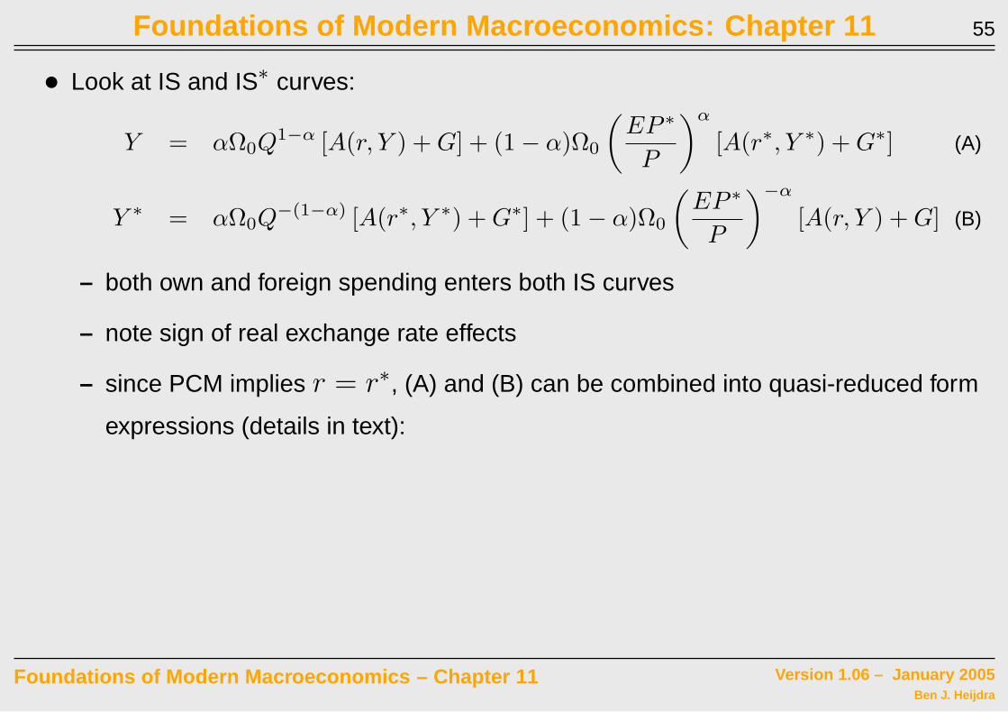
• Look at IS and IS∗ curves:
Y = αΩ0Q1−α [A(r, Y ) + G] + (1 − α)Ω0
(EP ∗
P
)α
[A(r∗, Y ∗) + G∗] (A)
Y ∗ = αΩ0Q−(1−α) [A(r∗, Y ∗) + G∗] + (1 − α)Ω0
(EP ∗
P
)−α
[A(r, Y ) + G] (B)
– both own and foreign spending enters both IS curves
– note sign of real exchange rate effects
– since PCM implies r = r∗, (A) and (B) can be combined into quasi-reduced form
expressions (details in text):
Foundations of Modern Macroeconomics – Chapter 11 Version 1.06 – January 2005Ben J. Heijdra

Foundations of Modern Macroeconomics: Chapter 11 56
Y = Ψ
[r∗−
, G++
, G∗
+, Q
+
]
Y ∗ = Φ
[r∗−
, G+, G∗
++, Q−
]
∗ own fiscal policy effect greater than spillover effect (assumed)
∗ interest rate effect same in both countries (via investment)
∗ real exchange rate effect different sign (for obvious reasons)
• From here on we work with logarithmic version of the two-country model. See Table
11.4.
Foundations of Modern Macroeconomics – Chapter 11 Version 1.06 – January 2005Ben J. Heijdra
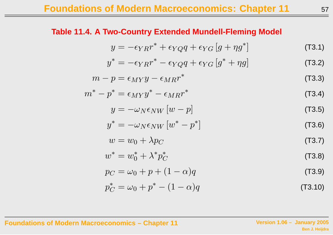
Foundations of Modern Macroeconomics: Chapter 11 57
Table 11.4. A Two-Country Extended Mundell-Fleming Model
y = −ǫY Rr∗ + ǫY Qq + ǫY G [g + ηg∗] (T3.1)
y∗ = −ǫY Rr∗ − ǫY Qq + ǫY G [g∗ + ηg] (T3.2)
m − p = ǫMY y − ǫMRr∗ (T3.3)
m∗ − p∗ = ǫMY y∗ − ǫMRr∗ (T3.4)
y = −ωN ǫNW [w − p] (T3.5)
y∗ = −ωN ǫNW [w∗ − p∗] (T3.6)
w = w0 + λpC (T3.7)
w∗ = w∗0 + λ∗p∗C (T3.8)
pC = ω0 + p + (1 − α)q (T3.9)
p∗C = ω0 + p∗ − (1 − α)q (T3.10)
Foundations of Modern Macroeconomics – Chapter 11 Version 1.06 – January 2005Ben J. Heijdra

Foundations of Modern Macroeconomics: Chapter 11 58
Economic Policy and the World Economy
• to build intuition we first look at some symmetric cases:
– nominal wage rigidity (NWR) in both countries
– real wage rigidity (RWR) in both countries
• next, we look at asymmetric case:
– NWR in foreign country (say the United States)
– RWR in domestic country (say Europe)
Foundations of Modern Macroeconomics – Chapter 11 Version 1.06 – January 2005Ben J. Heijdra
Foundations of Modern Macroeconomics: Chapter 11 59
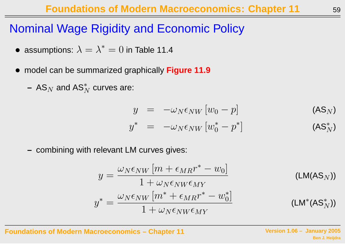
Nominal Wage Rigidity and Economic Policy
• assumptions: λ = λ∗ = 0 in Table 11.4
• model can be summarized graphically Figure 11.9
– ASN and AS∗N curves are:
y = −ωNǫNW [w0 − p] (ASN )
y∗ = −ωNǫNW [w∗0 − p∗] (AS∗
N )
– combining with relevant LM curves gives:
y =ωNǫNW [m + ǫMRr∗ − w0]
1 + ωNǫNW ǫMY
(LM(ASN ))
y∗ =ωNǫNW [m∗ + ǫMRr∗ − w∗
0]
1 + ωNǫNW ǫMY
(LM∗(AS∗N ))
Foundations of Modern Macroeconomics – Chapter 11 Version 1.06 – January 2005Ben J. Heijdra
Foundations of Modern Macroeconomics: Chapter 11 60
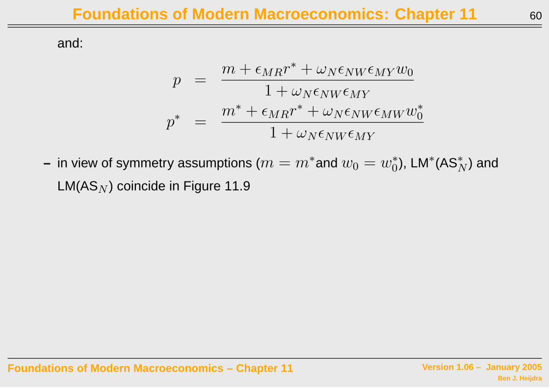
and:
p =m + ǫMRr∗ + ωNǫNW ǫMY w0
1 + ωNǫNW ǫMY
p∗ =m∗ + ǫMRr∗ + ωNǫNW ǫMW w∗
0
1 + ωNǫNW ǫMY
– in view of symmetry assumptions (m = m∗and w0 = w∗0), LM∗(AS∗
N ) and
LM(ASN ) coincide in Figure 11.9
Foundations of Modern Macroeconomics – Chapter 11 Version 1.06 – January 2005Ben J. Heijdra

Foundations of Modern Macroeconomics: Chapter 11 61
– combining LM(ASN ) with IS and LM∗(AS∗N ) with IS∗ yields:
r∗ =(1 + ωNǫNW ǫMY ) [ǫY Qq + ǫY G(g + ηg∗)]
ǫY R(1 + ωNǫNW ǫMY ) + ωNǫNW ǫMR
+ωNǫNW [w0 − m]
ǫY R(1 + ωNǫNW ǫMY ) + ωNǫNW ǫMR
(GMEN )
r∗ =(1 + ωNǫNW ǫMY ) [−ǫY Qq + ǫY G(g∗ + ηg)]
ǫY R(1 + ωNǫNW ǫMY ) + ωNǫNW ǫMR
+ωNǫNW [w∗
0 − m∗]
ǫY R(1 + ωNǫNW ǫMY ) + ωNǫNW ǫMR
(GME∗N )
– in Figure 11.9 these curves are drawn (notice slopes)
Foundations of Modern Macroeconomics – Chapter 11 Version 1.06 – January 2005Ben J. Heijdra

Foundations of Modern Macroeconomics: Chapter 11 62
• Fiscal Policy in Domestic Economy (g up)
– GMEN and GME∗N shift up (former by more if η < 1 “dominant own effect”)
– equilibrium from e0 to e1
– real exchange rate domestic economy appreciates
– output in both countries rises! Locomotive policy : one country drags itself and
the other country out of a recession (real wages fall)
• Fiscal Policy in Foreign Economy (g∗ up): exercise
– r∗ up; y and y∗ up by same amount
– Used below: ζ = ζ∗ = 1
Foundations of Modern Macroeconomics – Chapter 11 Version 1.06 – January 2005Ben J. Heijdra

Foundations of Modern Macroeconomics: Chapter 11 63
y, y* q1
!
!
LM(ASN) GMEN(g1)
e0
e1
q0
r*
q
!
!
e0
e1
y1 = y1* y0 = y0
*
GMEN(g0)
LM*(ASN)*
0
GMEN(g0)*
*GMEN(g1)
Figure 11.9: Fiscal Policy with Nominal Wage Rigidity in Both Countries
Foundations of Modern Macroeconomics – Chapter 11 Version 1.06 – January 2005Ben J. Heijdra

Foundations of Modern Macroeconomics: Chapter 11 64
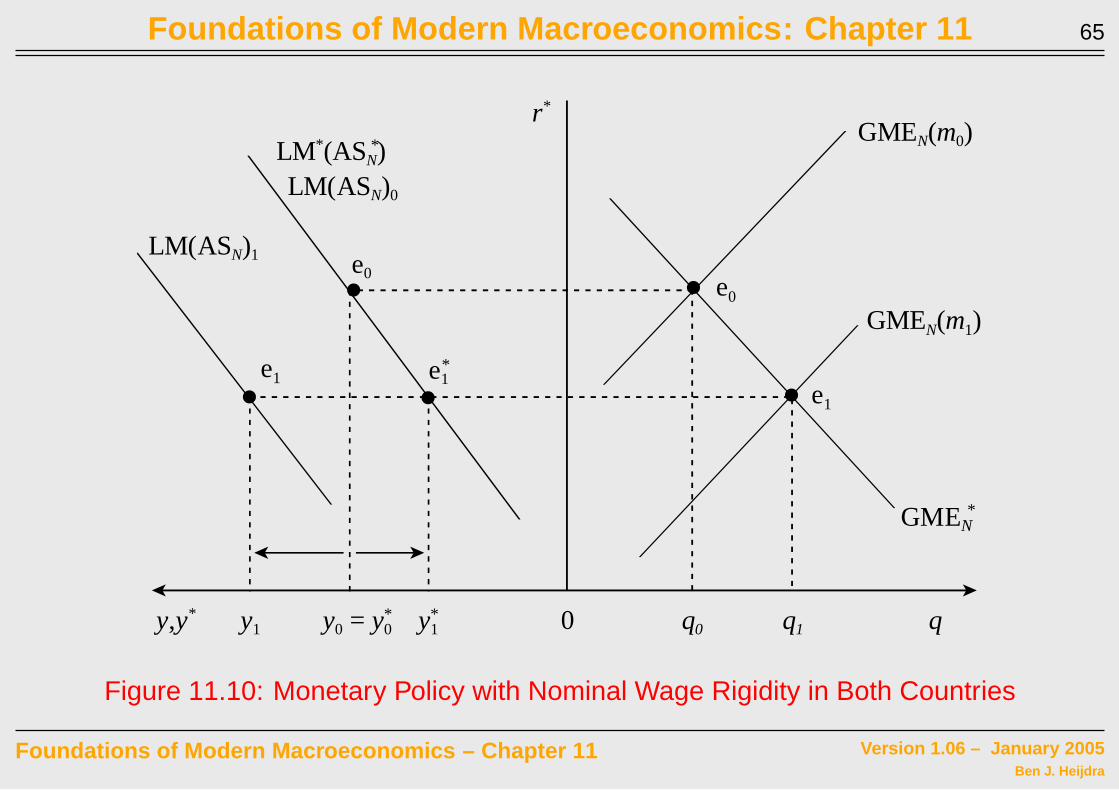
• Monetary Policy in Domestic Economy (m up)
– see Figure 11.10
– GMEN goes down
– LM(ASN ) to the left
– equilibrium from e0 to e1 in right-hand panel
– in left-hand panel, domestic economy from e0 to e1; foreign economy from e0 to
e∗1
– domestic economy gains at expense of foreign country: Beggar-Thy-Neighbour
Policy
• Monetary Policy in Foreign Economy (m∗ up): exercise
Foundations of Modern Macroeconomics – Chapter 11 Version 1.06 – January 2005Ben J. Heijdra
Foundations of Modern Macroeconomics: Chapter 11 65
y,y* q1
!
!
LM(ASN)1
GMEN(m0)
e0
e1
q0
r*
q
!
e0
e1
y1*y0 = y0
*
GMEN(m1)
y1
!!
0
e1*
LM*(ASN)*
LM(ASN)0
*GMEN
Figure 11.10: Monetary Policy with Nominal Wage Rigidity in Both Countries
Foundations of Modern Macroeconomics – Chapter 11 Version 1.06 – January 2005Ben J. Heijdra
Foundations of Modern Macroeconomics: Chapter 11 66
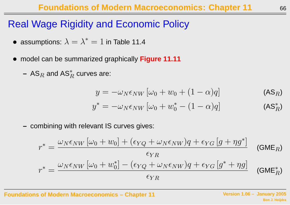
Real Wage Rigidity and Economic Policy
• assumptions: λ = λ∗ = 1 in Table 11.4
• model can be summarized graphically Figure 11.11
– ASR and AS∗R curves are:
y = −ωNǫNW [ω0 + w0 + (1 − α)q] (ASR)
y∗ = −ωNǫNW [ω0 + w∗0 − (1 − α)q] (AS∗
R)
– combining with relevant IS curves gives:
r∗ =ωNǫNW [ω0 + w0] + (ǫY Q + ωNǫNW )q + ǫY G [g + ηg∗]
ǫY R
(GMER)
r∗ =ωNǫNW [ω0 + w∗
0] − (ǫY Q + ωNǫNW )q + ǫY G [g∗ + ηg]
ǫY R
(GME∗R)
Foundations of Modern Macroeconomics – Chapter 11 Version 1.06 – January 2005Ben J. Heijdra

Foundations of Modern Macroeconomics: Chapter 11 67
• Fiscal Policy in Domestic Economy (g up)
– GMER and GME∗R shift up (former by more if η < 1 “dominant own effect”)
– equilibrium from e0 to e1
– real exchange rate domestic economy appreciates; interest rate rises
– output rises in domestic economy but falls in foreign economy!
Beggar-Thy-Neighbour Policy : the domestic expansion hurts the other country
(producer real wage falls domestically but rises abroad)
• Fiscal Policy in Foreign Economy (g∗ up): exercise
– y∗ up, y down.
– Used below: ζ = ζ∗ = −1
• Monetary Policy has no real effects: exercise
Foundations of Modern Macroeconomics – Chapter 11 Version 1.06 – January 2005Ben J. Heijdra

Foundations of Modern Macroeconomics: Chapter 11 68
y,y*
q1
!
!
GMER(g0)
e0
e1
q0
r*
q
!
e0
e1
y1*
y0 = y0*
GMER(g1)
y1
!
!
0
e1*
ASR*
ASR
GMER(g1)*
*GMER(g0)
Figure 11.11: Fiscal Policy with Real Wage Rigidity in Both Countries
Foundations of Modern Macroeconomics – Chapter 11 Version 1.06 – January 2005Ben J. Heijdra
Foundations of Modern Macroeconomics: Chapter 11 69
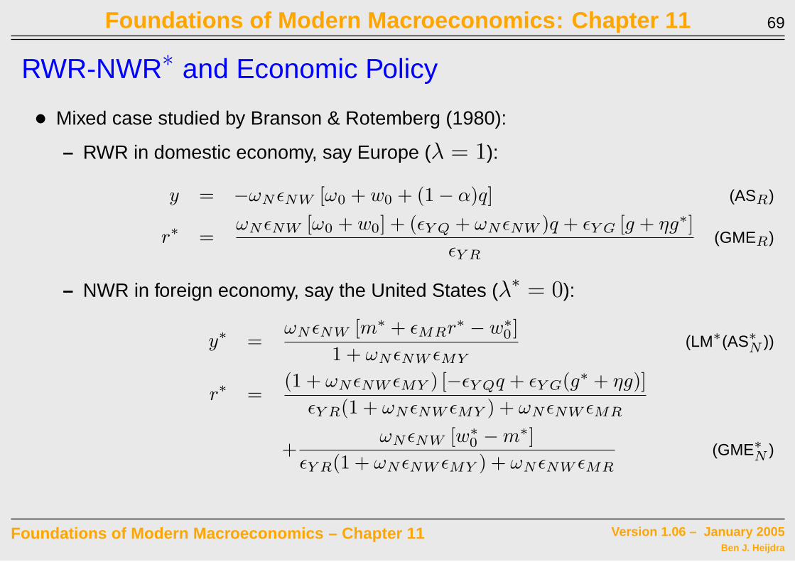
RWR-NWR∗ and Economic Policy
• Mixed case studied by Branson & Rotemberg (1980):
– RWR in domestic economy, say Europe (λ = 1):
y = −ωN ǫNW [ω0 + w0 + (1 − α)q] (ASR)
r∗ =ωN ǫNW [ω0 + w0] + (ǫY Q + ωN ǫNW )q + ǫY G [g + ηg∗]
ǫY R
(GMER)
– NWR in foreign economy, say the United States (λ∗ = 0):
y∗ =ωN ǫNW [m∗ + ǫMRr∗ − w∗
0 ]
1 + ωN ǫNW ǫMY
(LM∗(AS∗
N ))
r∗ =(1 + ωN ǫNW ǫMY ) [−ǫY Qq + ǫY G(g∗ + ηg)]
ǫY R(1 + ωN ǫNW ǫMY ) + ωN ǫNW ǫMR
+ωN ǫNW [w∗
0 − m∗]
ǫY R(1 + ωN ǫNW ǫMY ) + ωN ǫNW ǫMR
(GME∗
N )
Foundations of Modern Macroeconomics – Chapter 11 Version 1.06 – January 2005Ben J. Heijdra

Foundations of Modern Macroeconomics: Chapter 11 70
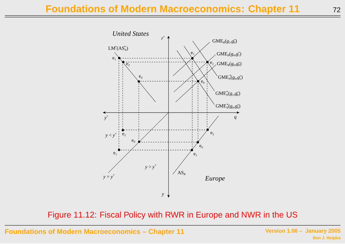
• Fiscal Policy in Domestic Economy (g up): see Figure 11.12
– GMER and GME∗N shift up (former by more if η < 1 “dominant own effect”)
– equilibrium from e0 to e1
– real exchange rate domestic economy appreciates; interest rate rises
– output rises in both economies. Locomotive Policy : the domestic expansion
benefits the other country (producer real wage falls domestically but rises abroad)
– Used below: 0 < ζ∗ < 1
Foundations of Modern Macroeconomics – Chapter 11 Version 1.06 – January 2005Ben J. Heijdra

Foundations of Modern Macroeconomics: Chapter 11 71
• Fiscal Policy in Foreign Economy (g∗ up): see Figure 11.12
– GMER and GME∗N shift up (latter by more if η < 1 “dominant own effect”)
– equilibrium from e0 to e2
– real exchange rate domestic economy depreciates; interest rate rises
– output falls in domestic economy but rises in the foreign economy!
Beggar-Thy-Neighbour Policy : the foreign expansion hurts the domestic
economy (real wage rises domestically but falls abroad)
– Used below: ζ < 0
Foundations of Modern Macroeconomics – Chapter 11 Version 1.06 – January 2005Ben J. Heijdra
Foundations of Modern Macroeconomics: Chapter 11 72
e0
e2
e1
!
GMER(g1,g0)*
United States
Europe
q
r*
y*
y
!
!
!
!
y = y*
y > y*
y < y*
e0
e0
e0
!
!!
!!e1 e1
! e2
e1
!e2
GMER(g0,g0)*
GMER(g0,g1)*
ASR
GMEN(g0,g0)* *
GMEN(g1,g0)* *
GMEN(g0,g1)* *
LM*(ASN)*
e2
Figure 11.12: Fiscal Policy with RWR in Europe and NWR in the US
Foundations of Modern Macroeconomics – Chapter 11 Version 1.06 – January 2005Ben J. Heijdra

Foundations of Modern Macroeconomics: Chapter 11 73
• Monetary Policy in Domestic Economy (m up) has no real effects
• Monetary Policy in Foreign Economy (m∗ up): see Figure 11.13
– GME∗N down and LM∗(AS∗
N ) to the left
– equilibrium from e0 to e1
– real exchange rate domestic economy appreciates; interest rate falls
– output rises in both economies (largest increase in domestic economy)!
Locomotive Policy : the foreign monetary expansion benefits the other country
(producer real wage falls in both countries)
Foundations of Modern Macroeconomics – Chapter 11 Version 1.06 – January 2005Ben J. Heijdra

Foundations of Modern Macroeconomics: Chapter 11 74
e0
e1
United States
Europe
q
r*
y*
y
!
!!
y = y*y > y*
y < y*
e0e0
e0!
!!e1 e1
e1
GMER
ASR
GMEN(m1)* *
GMEN(m0)* *
LM*(ASN)1*
!
!
LM*(ASN)0*
Figure 11.13: Monetary Policy with RWR in Europe and NWR in the US
Foundations of Modern Macroeconomics – Chapter 11 Version 1.06 – January 2005Ben J. Heijdra

Foundations of Modern Macroeconomics: Chapter 11 75
International Policy Coordination
• Policy question: is international coordination of policy welfare enhancing or not?
– international spillovers
– quantitative theory of economic policy [cf. Chapter 10]
• Summarize the insights from symmetric two-country model as follows:
y = g + ζg∗ (A)
y∗ = g∗ + ζ∗g (B)
– g and g∗ are indexes of fiscal policy
– NWR in both countries: ζ = ζ∗ = 1
– RWR in both countries: ζ = ζ∗ = −1
– RWR in home country, NWR in foreign country: ζ < 0 and 0 < ζ∗ < 1
Foundations of Modern Macroeconomics – Chapter 11 Version 1.06 – January 2005Ben J. Heijdra
Foundations of Modern Macroeconomics: Chapter 11 76
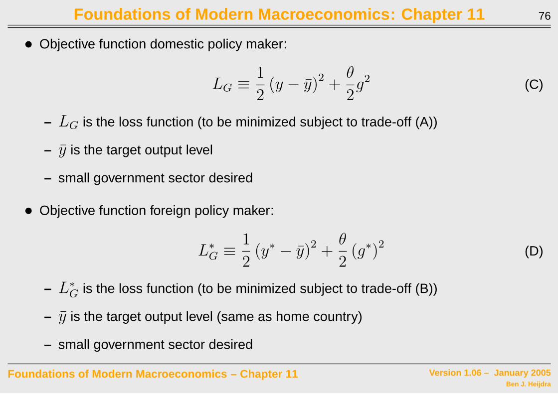
• Objective function domestic policy maker:
LG ≡1
2(y − y)2 +
θ
2g2 (C)
– LG is the loss function (to be minimized subject to trade-off (A))
– y is the target output level
– small government sector desired
• Objective function foreign policy maker:
L∗G ≡
1
2(y∗ − y)2 +
θ
2(g∗)2
(D)
– L∗G is the loss function (to be minimized subject to trade-off (B))
– y is the target output level (same as home country)
– small government sector desired
Foundations of Modern Macroeconomics – Chapter 11 Version 1.06 – January 2005Ben J. Heijdra

Foundations of Modern Macroeconomics: Chapter 11 77
Uncoordinated Fiscal Policy
• Policy makers choose own fiscal policy, ignoring international spill-overs
– Domestic policy maker chooses g to minimize LG subject to (A). FONC:
∂LG
∂g= (g + ζg∗ − y) + θg = 0 ⇒
g =y − ζg∗
1 + θ(RR)
– Foreign policy maker chooses g∗ to minimize L∗G subject to (B). FONC:
∂L∗G
∂g∗= (g∗ + ζ∗g − y) + θg∗ = 0 ⇒
g∗ =y − ζ∗g
1 + θ(RR∗)
– (RR) and (RR∗) are so-called reaction functions: a country’s best response, given
what the other country does.
Foundations of Modern Macroeconomics – Chapter 11 Version 1.06 – January 2005Ben J. Heijdra
Foundations of Modern Macroeconomics: Chapter 11 78
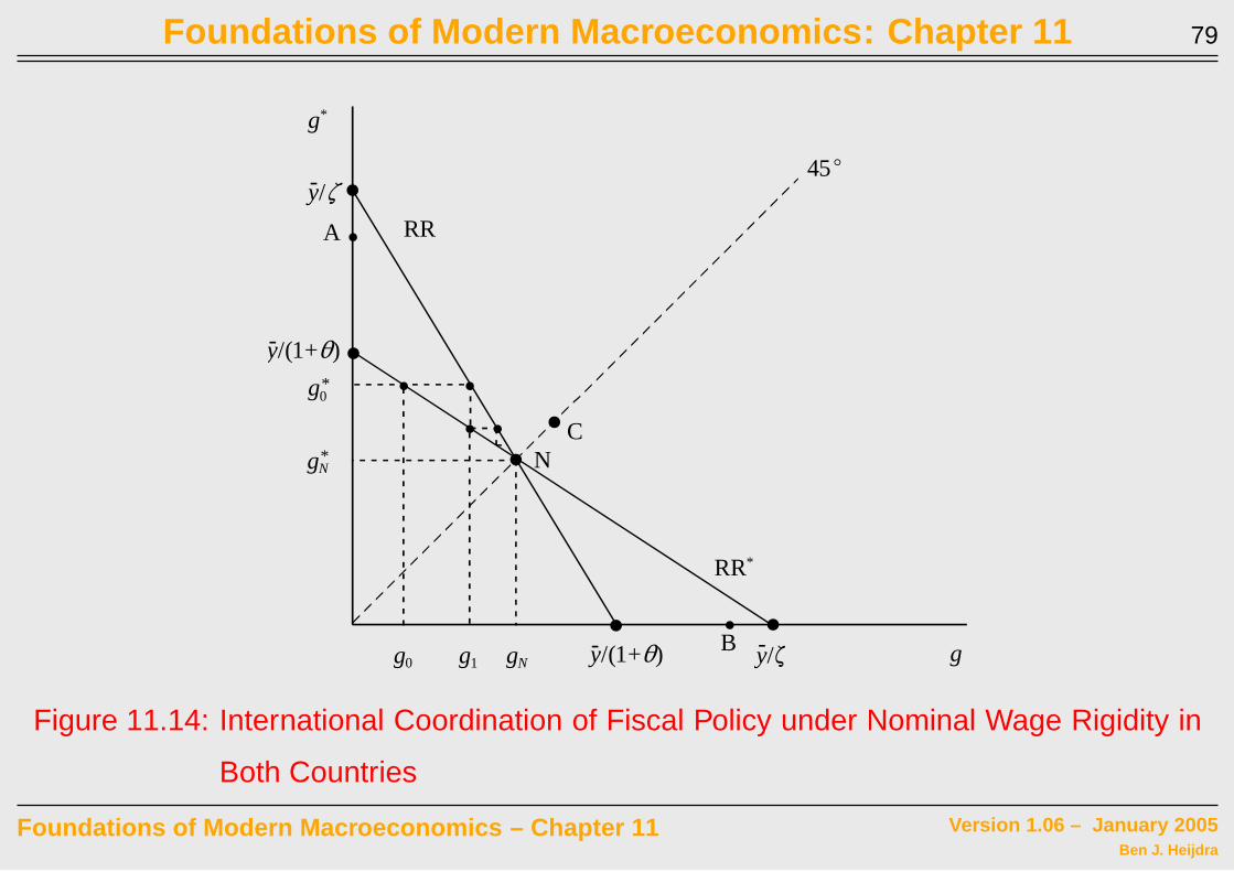
– see Figures 11.14-11.15 for the two pure cases. Non-cooperative Nash
Equilibrium is at the intersection of RR and RR∗
– for symmetric case (ζ = ζ∗) we have:
gN = g∗N =
y
1 + ζ + θ(Symmetric)
• NWR in both countries: ζ = ζ∗ = 1
– Figure 11.14 : reaction functions downward sloping
– unique non-cooperative Nash equilibrium at point N
– stable: possible sequence is g∗0 → g1 → g∗
1 → g2 → · · · g∗N−1 → gN
• RWR in both countries: ζ = ζ∗ < 0
– Figure 11.15 : reaction functions upward sloping
– unique stable non-cooperative Nash equilibrium at point N
Foundations of Modern Macroeconomics – Chapter 11 Version 1.06 – January 2005Ben J. Heijdra
Foundations of Modern Macroeconomics: Chapter 11 79
!
!
CN
RR*
RR
45E
g*
g
y/(1+2)-
y/.-
y/(1+2)- y/.-gN
gN*
g0
g0*
g1
! !
! !
! !
!
!
!
!
A
B
Figure 11.14: International Coordination of Fiscal Policy under Nominal Wage Rigidity in
Both Countries
Foundations of Modern Macroeconomics – Chapter 11 Version 1.06 – January 2005Ben J. Heijdra

Foundations of Modern Macroeconomics: Chapter 11 80
!
!
C
NRR*
RR45Eg*
gy/(1+2)-
y/(1+2)-!
!
Figure 11.15: International Coordination of Fiscal Policy under Real Wage Rigidity in Both
Countries
Foundations of Modern Macroeconomics – Chapter 11 Version 1.06 – January 2005Ben J. Heijdra

Foundations of Modern Macroeconomics: Chapter 11 81
Coordinated Fiscal Policy
• Is fiscal policy too expansionary?
• What would a coordinated fiscal policy look like?
• national policy makers give control over fiscal policy to international agency which
sets g and g∗ in order to minimize LG + L∗G subject to the trade-offs (A)-(B)
– formally:
ming∗,g
LG + L∗G ≡
1
2(g + ζg∗ − y)2 +
1
2(g∗ + ζ∗g − y)2
+θ
2g2 +
θ
2(g∗)2
Foundations of Modern Macroeconomics – Chapter 11 Version 1.06 – January 2005Ben J. Heijdra
Foundations of Modern Macroeconomics: Chapter 11 82
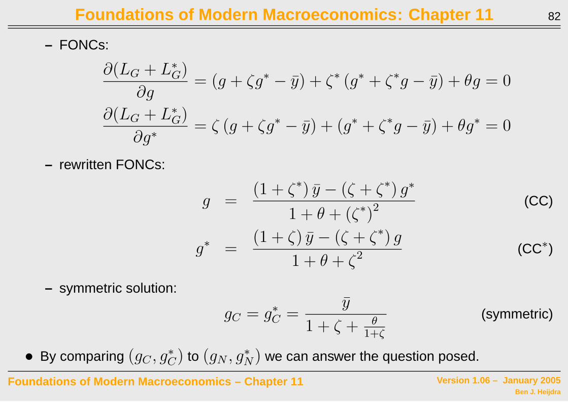
– FONCs:
∂(LG + L∗G)
∂g= (g + ζg∗ − y) + ζ∗ (g∗ + ζ∗g − y) + θg = 0
∂(LG + L∗G)
∂g∗= ζ (g + ζg∗ − y) + (g∗ + ζ∗g − y) + θg∗ = 0
– rewritten FONCs:
g =(1 + ζ∗) y − (ζ + ζ∗) g∗
1 + θ + (ζ∗)2 (CC)
g∗ =(1 + ζ) y − (ζ + ζ∗) g
1 + θ + ζ2 (CC∗)
– symmetric solution:
gC = g∗C =
y
1 + ζ + θ1+ζ
(symmetric)
• By comparing (gC , g∗C) to (gN , g∗
N) we can answer the question posed.
Foundations of Modern Macroeconomics – Chapter 11 Version 1.06 – January 2005Ben J. Heijdra

Foundations of Modern Macroeconomics: Chapter 11 83
• NWR in both countries: ζ = ζ∗ = 1
– gN < gC and g∗N < g∗
C (see Figure 11.14)
– too little spending in non-cooperative equilibrium
– fiscal policy is a locomotive policy; positive spill-over effect only taken into
account in coordinated policy
• RWR in both countries: ζ = ζ∗ = −1
– gN > gC and g∗N > g∗
C (see Figure 11.15)
– too much spending in non-cooperative equilibrium
– fiscal policy is a beggar-thy-neighbour policy; negative spill-over effect only taken
into account in coordinated policy
Foundations of Modern Macroeconomics – Chapter 11 Version 1.06 – January 2005Ben J. Heijdra
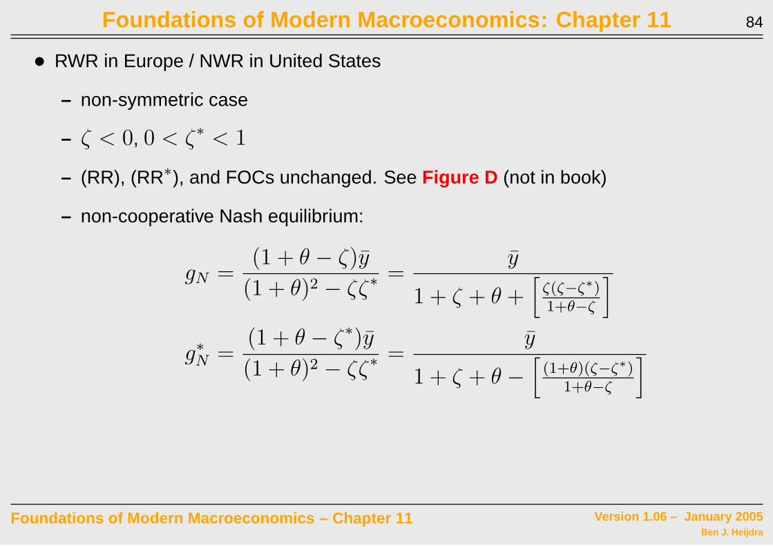
Foundations of Modern Macroeconomics: Chapter 11 84
• RWR in Europe / NWR in United States
– non-symmetric case
– ζ < 0, 0 < ζ∗ < 1
– (RR), (RR∗), and FOCs unchanged. See Figure D (not in book)
– non-cooperative Nash equilibrium:
gN =(1 + θ − ζ)y
(1 + θ)2 − ζζ∗ =y
1 + ζ + θ +[
ζ(ζ−ζ∗)1+θ−ζ
]
g∗N =
(1 + θ − ζ∗)y
(1 + θ)2 − ζζ∗ =y
1 + ζ + θ −[
(1+θ)(ζ−ζ∗)1+θ−ζ
]
Foundations of Modern Macroeconomics – Chapter 11 Version 1.06 – January 2005Ben J. Heijdra

Foundations of Modern Macroeconomics: Chapter 11 85
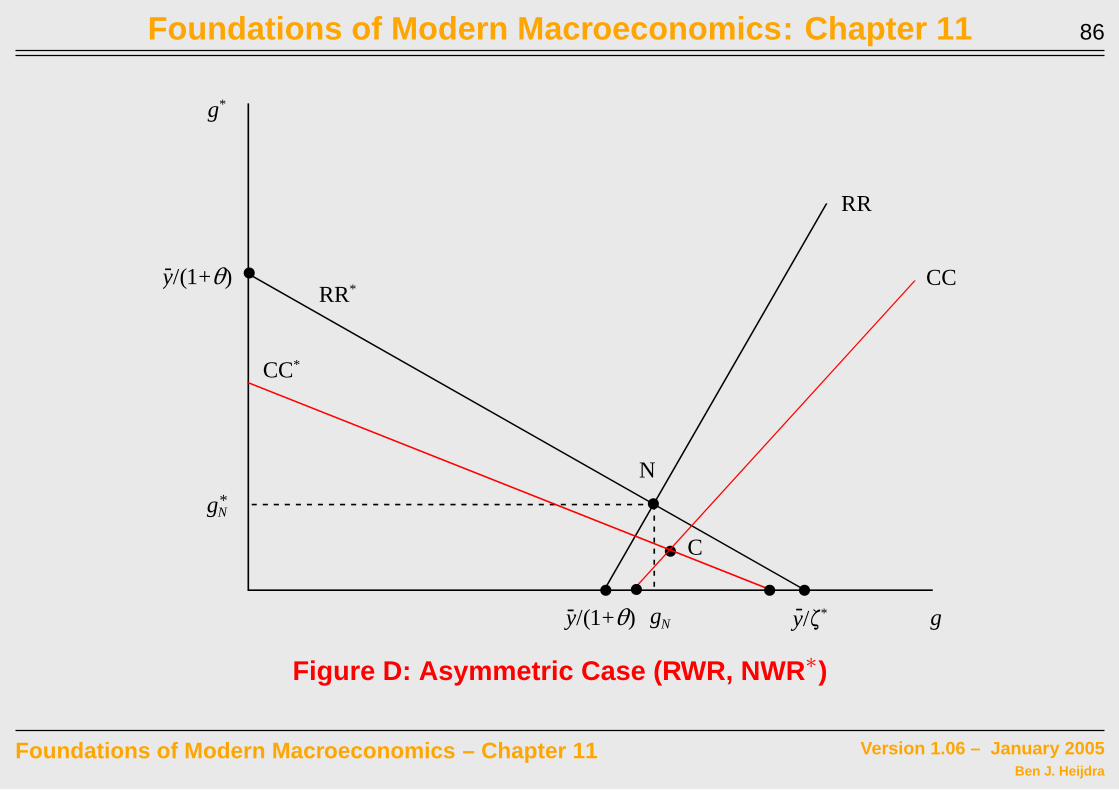
– comparison:
gC > gN
g∗C < g∗
N
– intuition:
∗ in absence of coordination, Europe spends too little (locomotive) and the US
spends too much (beggar-thy-neighbour)
∗ interest rate too high, dollar too strong, unemployment in Europe too high
(conclusion not relevant in 2005 but was deemed relevant in early 1980s)
Foundations of Modern Macroeconomics – Chapter 11 Version 1.06 – January 2005Ben J. Heijdra
Foundations of Modern Macroeconomics: Chapter 11 86
!
!
C
N
RR*
RR
g*
g
y/(1+2)-
y/(1+2)- y/.*-gN
gN*
!
!
! CC
! !
CC*
Figure D: Asymmetric Case (RWR, NWR ∗)
Foundations of Modern Macroeconomics – Chapter 11 Version 1.06 – January 2005Ben J. Heijdra
Foundations of Modern Macroeconomics: Chapter 11 87
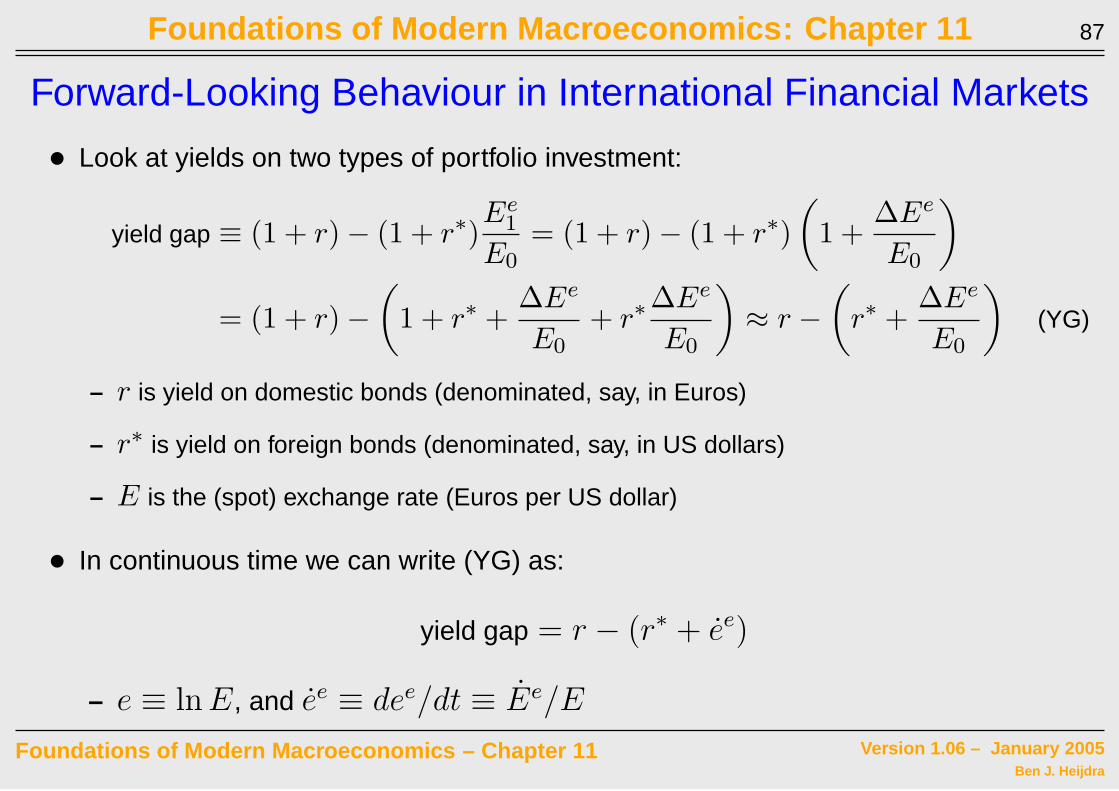
Forward-Looking Behaviour in International Financial Markets
• Look at yields on two types of portfolio investment:
yield gap ≡ (1 + r) − (1 + r∗)Ee
1
E0= (1 + r) − (1 + r∗)
(1 +
∆Ee
E0
)
= (1 + r) −
(1 + r∗ +
∆Ee
E0+ r∗
∆Ee
E0
)≈ r −
(r∗ +
∆Ee
E0
)(YG)
– r is yield on domestic bonds (denominated, say, in Euros)
– r∗ is yield on foreign bonds (denominated, say, in US dollars)
– E is the (spot) exchange rate (Euros per US dollar)
• In continuous time we can write (YG) as:
yield gap = r − (r∗ + ee)
– e ≡ ln E, and ee ≡ dee/dt ≡ Ee/E
Foundations of Modern Macroeconomics – Chapter 11 Version 1.06 – January 2005Ben J. Heijdra

Foundations of Modern Macroeconomics: Chapter 11 88
• Arbitrage in world financial marlets will ensure that like assets will earn like yields,
i.e. uncovered interest parity holds:
r = r∗ + ee (UIP)
• Under flexible exchange rates the agents must form an expectation regarding future
exchange rates:
– so far we have used the assumption of inelastic expectations:
ee = 0 (SEH)
– from here on we will use the perfect foresight hypothesis:
ee = e (PFH)
• Rudiger Dornbusch (1942-2002) added (UIP) and (PFH) to the IS-LM model and
investigated the effects of monetary and fiscal policy
Foundations of Modern Macroeconomics – Chapter 11 Version 1.06 – January 2005Ben J. Heijdra
Foundations of Modern Macroeconomics: Chapter 11 89
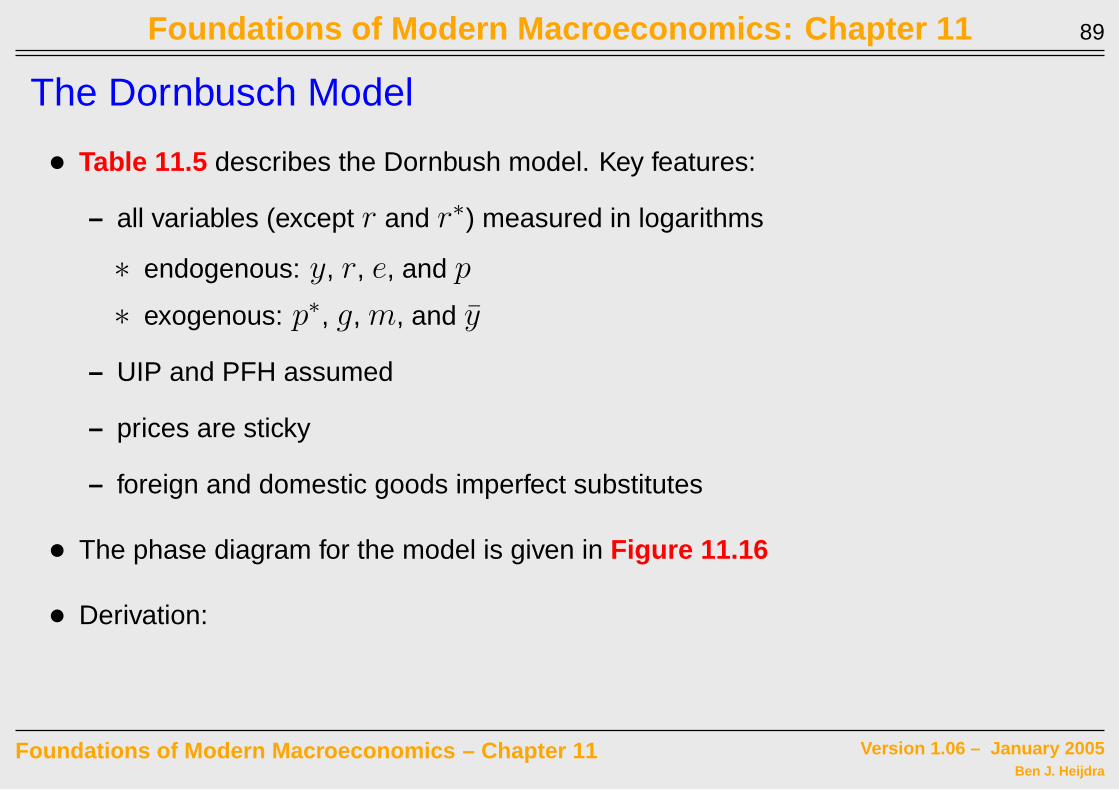
The Dornbusch Model
• Table 11.5 describes the Dornbush model. Key features:
– all variables (except r and r∗) measured in logarithms
∗ endogenous: y, r, e, and p
∗ exogenous: p∗, g, m, and y
– UIP and PFH assumed
– prices are sticky
– foreign and domestic goods imperfect substitutes
• The phase diagram for the model is given in Figure 11.16
• Derivation:
Foundations of Modern Macroeconomics – Chapter 11 Version 1.06 – January 2005Ben J. Heijdra
Foundations of Modern Macroeconomics: Chapter 11 90
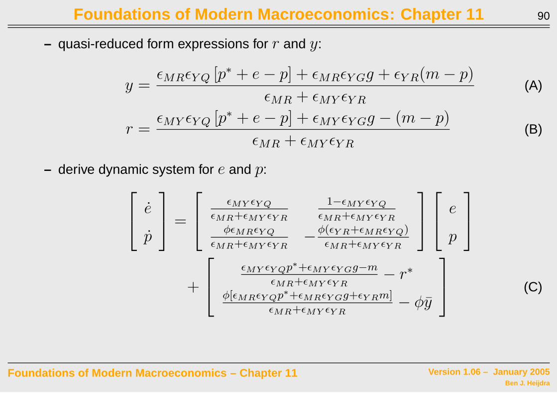
– quasi-reduced form expressions for r and y:
y =ǫMRǫY Q [p∗ + e − p] + ǫMRǫY Gg + ǫY R(m − p)
ǫMR + ǫMY ǫY R
(A)
r =ǫMY ǫY Q [p∗ + e − p] + ǫMY ǫY Gg − (m − p)
ǫMR + ǫMY ǫY R
(B)
– derive dynamic system for e and p: e
p
=
ǫMY ǫY Q
ǫMR+ǫMY ǫY R
1−ǫMY ǫY Q
ǫMR+ǫMY ǫY R
φǫMRǫY Q
ǫMR+ǫMY ǫY R−
φ(ǫY R+ǫMRǫY Q)
ǫMR+ǫMY ǫY R
e
p
+
ǫMY ǫY Qp∗+ǫMY ǫY Gg−m
ǫMR+ǫMY ǫY R− r∗
φ[ǫMRǫY Qp∗+ǫMRǫY Gg+ǫY Rm]
ǫMR+ǫMY ǫY R− φy
(C)
Foundations of Modern Macroeconomics – Chapter 11 Version 1.06 – January 2005Ben J. Heijdra
Foundations of Modern Macroeconomics: Chapter 11 91
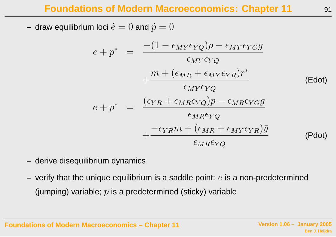
– draw equilibrium loci e = 0 and p = 0
e + p∗ =−(1 − ǫMY ǫY Q)p − ǫMY ǫY Gg
ǫMY ǫY Q
+m + (ǫMR + ǫMY ǫY R)r∗
ǫMY ǫY Q
(Edot)
e + p∗ =(ǫY R + ǫMRǫY Q)p − ǫMRǫY Gg
ǫMRǫY Q
+−ǫY Rm + (ǫMR + ǫMY ǫY R)y
ǫMRǫY Q
(Pdot)
– derive disequilibrium dynamics
– verify that the unique equilibrium is a saddle point: e is a non-predetermined
(jumping) variable; p is a predetermined (sticky) variable
Foundations of Modern Macroeconomics – Chapter 11 Version 1.06 – January 2005Ben J. Heijdra
Foundations of Modern Macroeconomics: Chapter 11 92
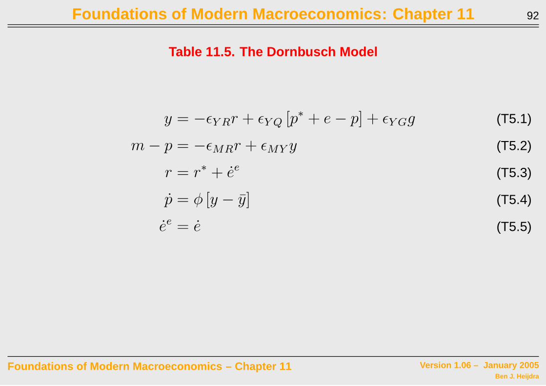
Table 11.5. The Dornbusch Model
y = −ǫY Rr + ǫY Q [p∗ + e − p] + ǫY Gg (T5.1)
m − p = −ǫMRr + ǫMY y (T5.2)
r = r∗ + ee (T5.3)
p = φ [y − y] (T5.4)
ee = e (T5.5)
Foundations of Modern Macroeconomics – Chapter 11 Version 1.06 – January 2005Ben J. Heijdra

Foundations of Modern Macroeconomics: Chapter 11 93
e = 0.
p = 0.
e
p
!
!
A
AN
B
a0
!
C
CN!
!
BN!
!
!
!
D
DNSP
e0
p0
Figure 11.16: Phase Diagram for the Dornbusch Model
Foundations of Modern Macroeconomics – Chapter 11 Version 1.06 – January 2005Ben J. Heijdra

Foundations of Modern Macroeconomics: Chapter 11 94
Economic Policy in the Dornbusch Model
• Under PFH timing of policy is crucial (as in perfect foresight models of Chapter 4)
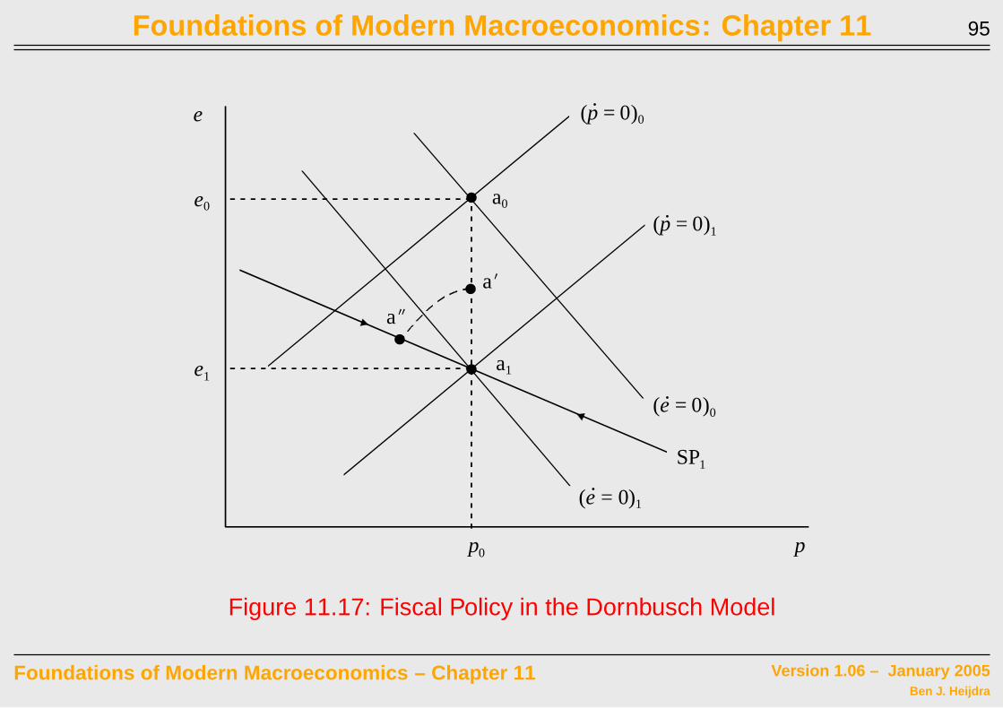
• Fiscal policy: unanticipated / permanent increase in g
– see Figure 11.17
– e = 0 and p = 0 shift down
– equilibrium from a0 to a1; immediate appreciation of currency
– no price change and no transitional dynamics
– conclusion same as standard Mundell-Fleming model
• Fiscal policy: anticipated / permanent increase in g
– heuristic solution principle of Chapter 4
– adjustment path jump from a0 to a′, gradual move from a′ to a′′ and then to a1
– intuition: self-test
Foundations of Modern Macroeconomics – Chapter 11 Version 1.06 – January 2005Ben J. Heijdra
Foundations of Modern Macroeconomics: Chapter 11 95
e
p
!
aN
a0!
!
!
SP1
e1
p0
aO
a1
(e = 0)1
.
(e = 0)0
.
(p = 0)0
.
(p = 0)1
.e0
Figure 11.17: Fiscal Policy in the Dornbusch Model
Foundations of Modern Macroeconomics – Chapter 11 Version 1.06 – January 2005Ben J. Heijdra

Foundations of Modern Macroeconomics: Chapter 11 96
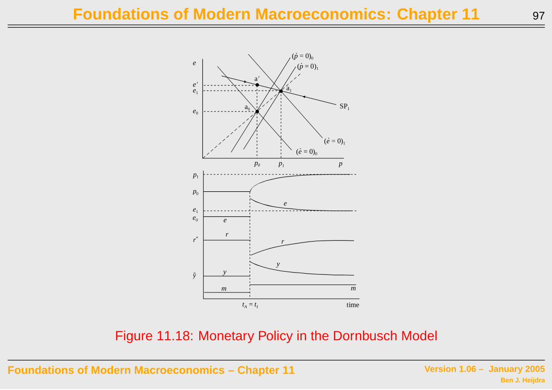
• Monetary policy: unanticipated / permanent increase in m
– see Figure 11.18
– e = 0 and p = 0 to the right
– long-run equilibrium from a0 to a1 (real exchange rate unaffected in long run)
– transitional dynamics: impact jump from a0 to a′; thereafter gradual move from a′
to a1
– conclusion: the nominal exchange rate overshoots its long-run value in the short
run! intuition for overshooting:
∗ agents expect long-run depreciation of currency (e from e0 to e1)
∗ domestic assets less attractive, at impact r ↓ (net capital outflow) and e ↑
∗ during transition investors must be compensated for r < r∗ by appreciating
exchange rate (e < 0)
• Monetary policy: anticipated / permanent increase in m: self-test
Foundations of Modern Macroeconomics – Chapter 11 Version 1.06 – January 2005Ben J. Heijdra
Foundations of Modern Macroeconomics: Chapter 11 97
p0
rr
m
p1
tA = tI time
a1!
!
p0 p1 p
e
SP1
!
yy
.(e = 0)1
.(e = 0)0
a0
aN
e0
eNe1
.(p = 0)0
.(p = 0)1
e
e
m
e1
e0
y-
r*
Figure 11.18: Monetary Policy in the Dornbusch Model
Foundations of Modern Macroeconomics – Chapter 11 Version 1.06 – January 2005Ben J. Heijdra

Foundations of Modern Macroeconomics: Chapter 11 98
Overshooting: Sensitivity Analysis
• What are the key assumptions leading to the overshooting result?
– role of price stickiness?
– role of imperfect capital mobility?
– role of monetary accommodation?
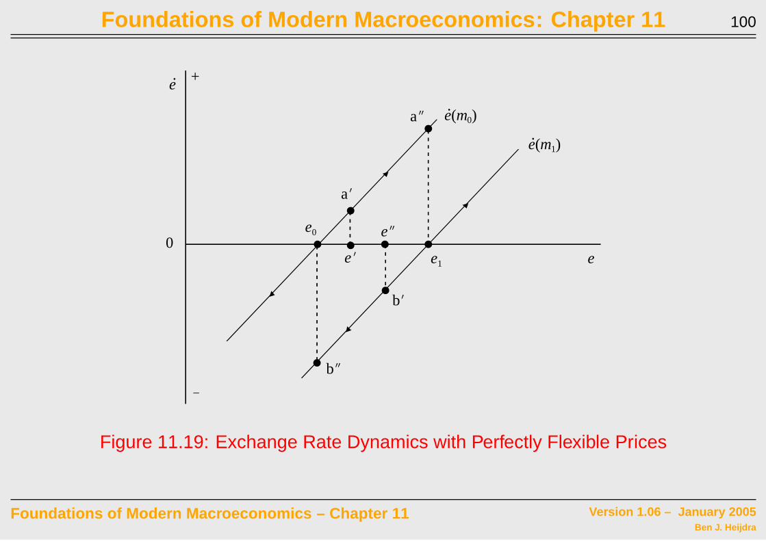
• Perfectly Flexible Prices in the Dornbush model
– φ → ∞, so y = y always
– domestic interest rate:
r =(ǫY QǫMY − 1)y + ǫY Q(p∗ + e) + ǫY Gg − ǫY Qm
ǫY R + ǫY QǫMR
Foundations of Modern Macroeconomics – Chapter 11 Version 1.06 – January 2005Ben J. Heijdra

Foundations of Modern Macroeconomics: Chapter 11 99
– (unstable) differential equation for e:
e =(ǫY QǫM − 1)y + ǫY Q(p∗ + e) + ǫY Gg − ǫY Qm
ǫY R + ǫY QǫMR
− r∗
– unanticipated / permanent increase in m results in a once-off increase in e
(depreciation): no overshooting!
– see Figure 11.19
Foundations of Modern Macroeconomics – Chapter 11 Version 1.06 – January 2005Ben J. Heijdra
Foundations of Modern Macroeconomics: Chapter 11 100
e0 !
!
!
e. +
!
e0
e1
e(m1).
e(m0).
eN
eO
!
!!
!
!
aN
aO
bN
bO
Figure 11.19: Exchange Rate Dynamics with Perfectly Flexible Prices
Foundations of Modern Macroeconomics – Chapter 11 Version 1.06 – January 2005Ben J. Heijdra

Foundations of Modern Macroeconomics: Chapter 11 101
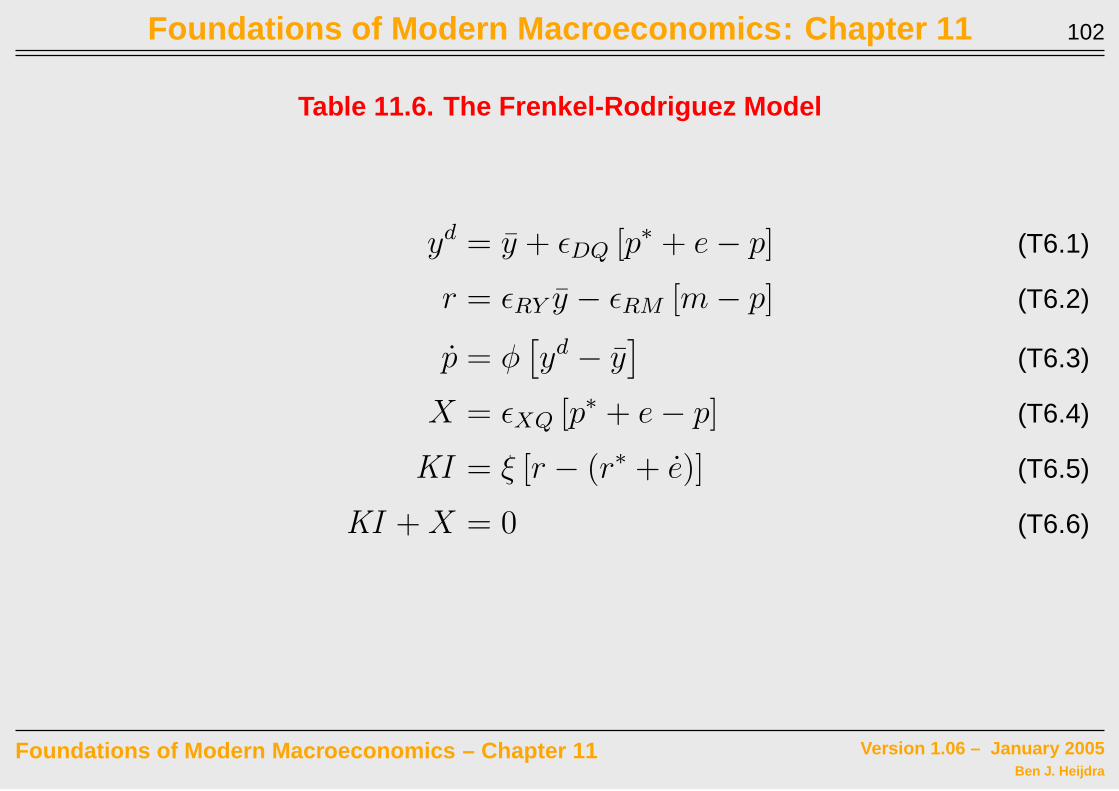
• Imperfect Capital Mobility in the Dornbusch model
– Frenkel & Rodriguez (1982)
– model given in Table 11.6
– phase diagram with low capital mobility in Figure 11.20 : no overshooting
– phase diagram with high capital mobility in Figure 11.21 : overshooting
– lesson: sticky prices necessary but not sufficient condition for overshooting result
to occur
Foundations of Modern Macroeconomics – Chapter 11 Version 1.06 – January 2005Ben J. Heijdra
Foundations of Modern Macroeconomics: Chapter 11 102
Table 11.6. The Frenkel-Rodriguez Model
yd = y + ǫDQ [p∗ + e − p] (T6.1)
r = ǫRY y − ǫRM [m − p] (T6.2)
p = φ[yd − y
](T6.3)
X = ǫXQ [p∗ + e − p] (T6.4)
KI = ξ [r − (r∗ + e)] (T6.5)
KI + X = 0 (T6.6)
Foundations of Modern Macroeconomics – Chapter 11 Version 1.06 – January 2005Ben J. Heijdra
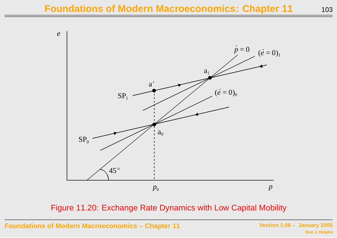
Foundations of Modern Macroeconomics: Chapter 11 103
e
p
!
aN
a0
!
!
SP0
p0
a1
(e = 0)1
.
(e = 0)0
.
p = 0.
SP1
45E
Figure 11.20: Exchange Rate Dynamics with Low Capital Mobility
Foundations of Modern Macroeconomics – Chapter 11 Version 1.06 – January 2005Ben J. Heijdra
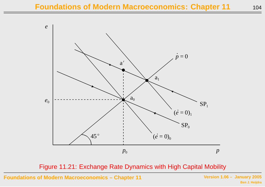
Foundations of Modern Macroeconomics: Chapter 11 104
e
p
!
aN
a0
!
!
SP1
p0
a1
(e = 0)1
.
(e = 0)0
.
p = 0.
e0
SP0
45E
Figure 11.21: Exchange Rate Dynamics with High Capital Mobility
Foundations of Modern Macroeconomics – Chapter 11 Version 1.06 – January 2005Ben J. Heijdra

Foundations of Modern Macroeconomics: Chapter 11 105
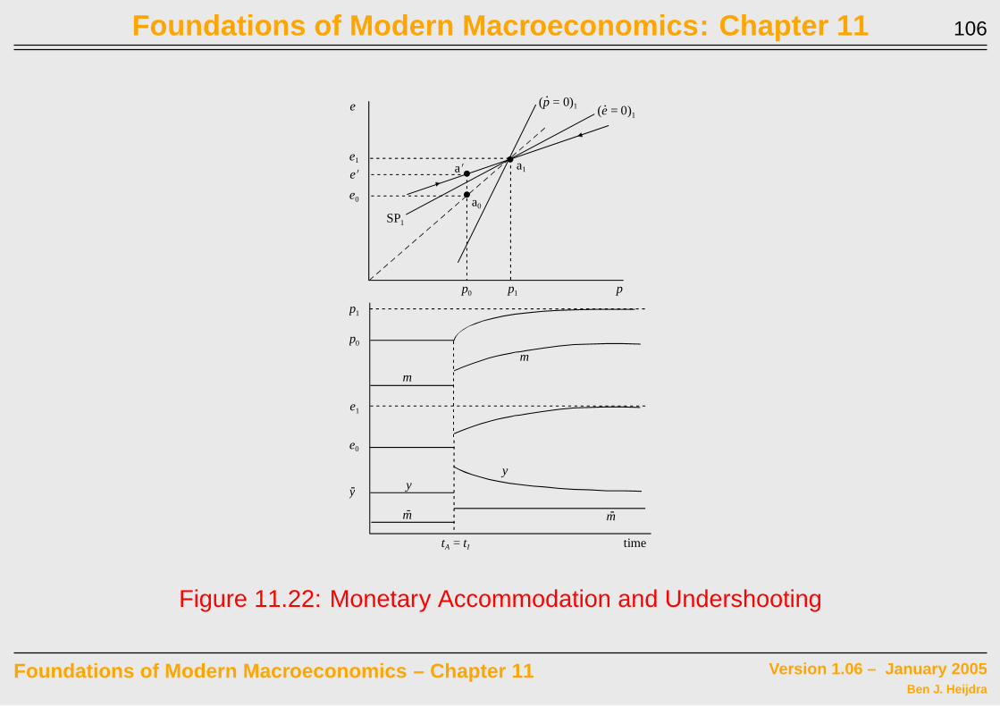
• Monetary Accommodation in the Dornbusch model
– policy maker may accommodate price shocks:
m = m + δp
∗ δ = 0 in Dornbush model (“pure float” of the exchange rate)
∗ 0 < δ < 1 here (“dirty float”)
– phase diagram with no accommodation in Figure 11.18: overshooting
– phase diagram with strong accommodation (δ high) in Figure 11.22 : no
overshooting
– lesson: by engaging in monetary accommodation, the policy maker can prevent
overshooting to occur
Foundations of Modern Macroeconomics – Chapter 11 Version 1.06 – January 2005Ben J. Heijdra
Foundations of Modern Macroeconomics: Chapter 11 106
p0
p1
tA = tI time
a1!
!
p0 p1 p
e
SP1
!
yy
.(e = 0)1
a0
aN
e0
eN
e1
.(p = 0)1
m
m-
e1
e0
y-
m-
m
Figure 11.22: Monetary Accommodation and Undershooting
Foundations of Modern Macroeconomics – Chapter 11 Version 1.06 – January 2005Ben J. Heijdra

Foundations of Modern Macroeconomics: Chapter 11 107
Punchlines
• crucial aspects open economy:
– financial openness
– type of exchange rate system
• effects of fiscal and monetary policy depend on both aspects
• from the supply side another aspect is highlighted: the wage setting rule
• in a two-country setting, shocks generally spill over across countries
• coordinated policy is generally different from uncoordinated policy
– direction of change depends on wage setting rule in place
– (positive or negative) spill-overs internalized
Foundations of Modern Macroeconomics – Chapter 11 Version 1.06 – January 2005Ben J. Heijdra

Foundations of Modern Macroeconomics: Chapter 11 108
• forward-looking sticky-price model with perfect capital mobility
– overshooting: financial shocks cause volatility
– determinants of overshooting
Foundations of Modern Macroeconomics – Chapter 11 Version 1.06 – January 2005Ben J. Heijdra