Forward and Inverse Forward and Inverse Modeling Modeling

of Atmospheric COof Atmospheric CO22

Scott Denning, Nick Parazoo, Kathy Corbin, Marek Uliasz, Andrew Schuh, Dusanka Zupanski, Ken Davis, and Peter Rayner

Acknowledgements:Support by US NOAA, NASA, DoE

Signal? Noise? Which is which?Signal? Noise? Which is which?

Cape Grim

Usual approach is to exclude“spikes” as non-“background”

Law et al inverted the “spikes” instead!

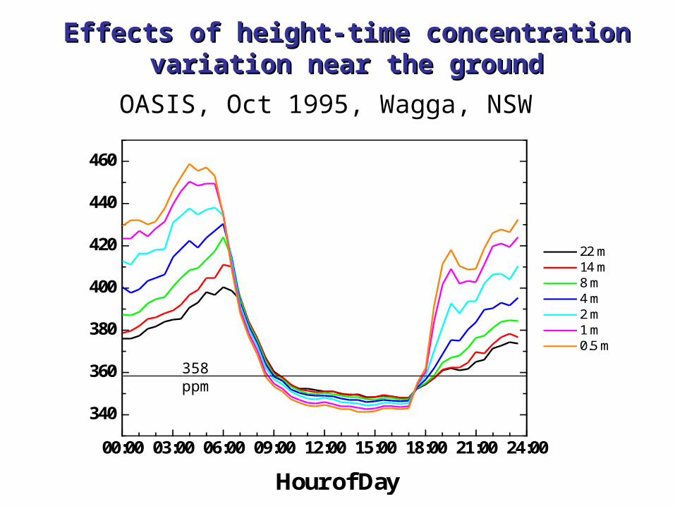
Effects of height-time concentration Effects of height-time concentration variation near the groundvariation near the ground

00:00 03:00 06:00 09:00 12:00 15:00 18:00 21:00 24:00

340

360

380

400

420

440

460

22 m 14 m 8 m 4 m 2 m 1 m 0.5 m

Hour of Day

358 ppm

OASIS, Oct 1995, Wagga, NSW

Continental NEE and [COContinental NEE and [CO22]]

• Variance in [CO2] is strongly dominated by diurnal and seasonal cycles, but target is source/sink processes on interannual to decadal time scales

• Diurnal variations are controlled locally by nocturnal stability (variations in ecosystem resp are secondary!)

• Seasonal variations are controlled hemispherically by phenology

• Synoptic variations controlled regionally, over scales of 100 - 1000 km. Let’s target these.

wplsobs

frs

sgp

wkt

hrv

amtlef

ring

Seasonal and Synoptic Seasonal and Synoptic VariationsVariations

• Strong coherent seasonal cycle across stations

• SGP shows earlier drawdown (winter wheat), then relaxes to hemispheric signal

• Synoptic variance of 10-20 ppm, strongest in summer

• Events can be traced across multiple sites

• What causes these huge coherent changes?

Daily min [CO2], 2004

Modeling & Analysis ToolsModeling & Analysis Tools(alphabet soup)(alphabet soup)

• Ecosystem model (Simple Biosphere, SiB)

• Weather and atmospheric transport (Regional Atmospheric Modeling System, RAMS)

• Large-scale continental inflow (Parameterized Chemical Transport Model, PCTM)

• Airmass trajectories(Lagrangian Particle Dispersion Model, LPDM)

• Optimization procedure to estimate persistent model biases upstream (Maximum Likelihood Ensemble Filter, MLEF)

Frontal Composites of Frontal Composites of WeatherWeather

GGρ =∇ρg∇∇ρ

• The time at which magnitude of gradient of density (ρ) changes the most rapidly defines the trough (minimum GG ρ, cold front) and ridge (maximum GG)

Frontal Locator Function

Oklahoma Wisconsin Alberta

Frontal COFrontal CO22 “Climatology”“Climatology” • Multiple cold fronts

averaged together (diurnal & seasonal cycle removed)

• Some sites show frontal drop in CO2, some show frontal rise … controls?

• Simulated shape and phase similar to observations

• What causes these?

wplsobs

frs

sgp

wkt

hrv

amtlef

ring

Deformational FlowDeformational Flow

• Anomalies organize along cold front

• dC/dx ~ 15ppm/3-5°

Dg

Dt

∂C∂x

+∂C∂y

⎛⎝⎜

⎞⎠⎟=−

∂ug

∂x∂C∂x

+∂vg

∂x∂C∂y

⎛⎝⎜

⎞⎠⎟−

∂ug

∂y∂C∂x

+∂vg

∂y∂C∂y

⎛⎝⎜

⎞⎠⎟

shear deformation- tracer field rotated by shear vorticity

stretching deformation- tracer field deformed by stretching

gradientstrength

ΔC

Δt= u

ΔC

Δx→ C day+1 =

uΔtΔC

Δx=

5ms−1 * 3600s * 24hr *15 ppm

5° *100km= 12 ppm

Lateral Boundary ForcingLateral Boundary Forcing

• Flask sampling shows N-S gradients of 5-10 ppm in [CO2] over Atlantic and Pacific

• Synoptic waves (weather) drive quasi-periodic reversals in meridional (v) wind with ~5 day frequency

• Expect synoptic variations of ~ 5 ppm over North America, unrelated to NEE!

• Regional inversions must specify correct time-varying lateral boundary conditions

• Sensitivity exp: turn off all NEE in Western Hemisphere, analyze CO2(t)

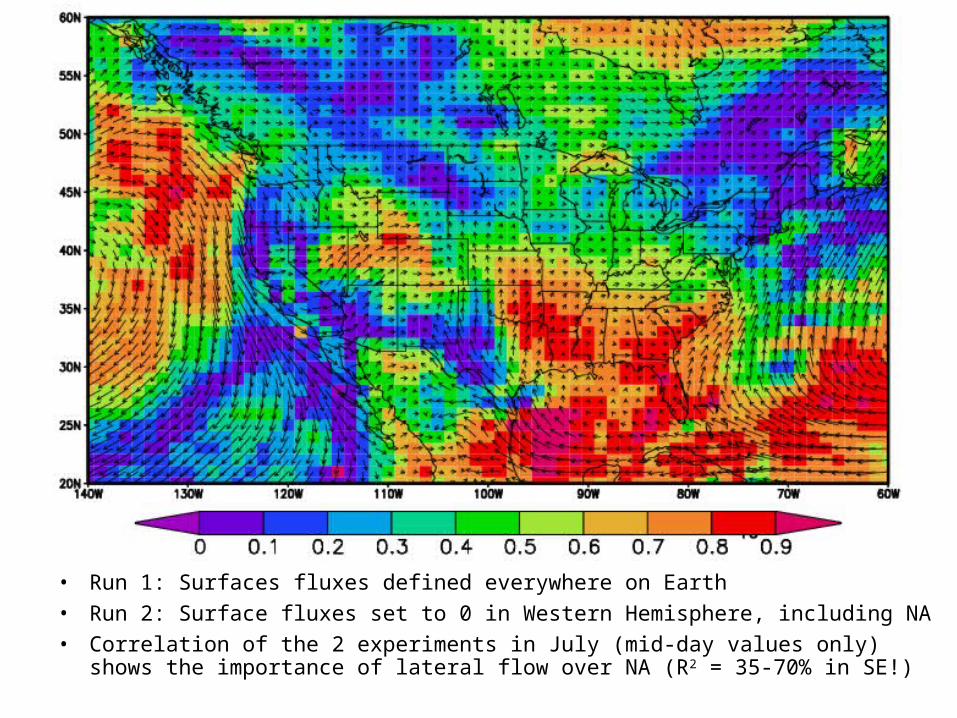
• Run 1: Surfaces fluxes defined everywhere on Earth• Run 2: Surface fluxes set to 0 in Western Hemisphere, including NA• Correlation of the 2 experiments in July (mid-day values only) shows

the importance of lateral flow over NA (R2 = 35-70% in SE!)

Regional Fluxes are Hard!Regional Fluxes are Hard!

• Eddy covariance flux footprint is only a few hundred meters upwind

• Heterogeneity of fluxes too fine-grained to be captured, even by many flux towers– Temporal variations ~ hours to days– Spatial variations in annual mean ~ 1 km

• Some have tried to “paint by numbers,” – measure flux in a few places and then apply

everywhere else using remote sensing

• Annual source/sink isn’t a result of vegetation type or LAI, but rather a complex mix of management history, soils, nutrients, topography not easily seen by RS

A Different StrategyA Different Strategy• Divide carbon balance into “fast” processes that

we know how to model, and “slow” processes that we don’t

• Use coupled model to simulate fluxes and resulting atmospheric CO2

• Measure real CO2 variations• Figure out where the air has been • Use mismatch between simulated and observed

CO2 to “correct” persistent model biases

• GOAL: Time-varying maps of sources/sinks consistent with observed vegetation, fluxes, and CO2 as well as process knowledge

FCO2 (x, y, t) =R(x,y,t)−GPP(x,y,t)

Treatment of Variations for Treatment of Variations for InversionInversion

• Fine-scale variations (hourly, pixel-scale) from weather forcing, NDVI as processed by forward model logic (SiB-RAMS)

• Multiplicative biases (caused by “slow” BGC that’s not in the model) derived by from observed hourly [CO2]

FCO2 (x, y, t) =βR(x,y)R(x,y,t)−βGPP (x,y)GPP(x,y,t)

SiB SiB

unknown!

unknown!

Ck ,m = βR,i, jRi, j ,nCRk,m,i, j ,n* + βA,i, jAi, j ,nCAk,m,i, j ,n

*( )i, j ,n∑ ΔtfΔxΔy+ CIN

Flux-convolved influence functions derived from SiB-RAMS

Average NEESiB-RAMS Simulated Net Ecosystem Exchange (NEE)SiB-RAMS Simulated Net Ecosystem Exchange (NEE)

QuickTime™ and aPNG decompressor

are needed to see this picture.

Filtered: diurnal cycle removed

Filtered: diurnal cycle removed

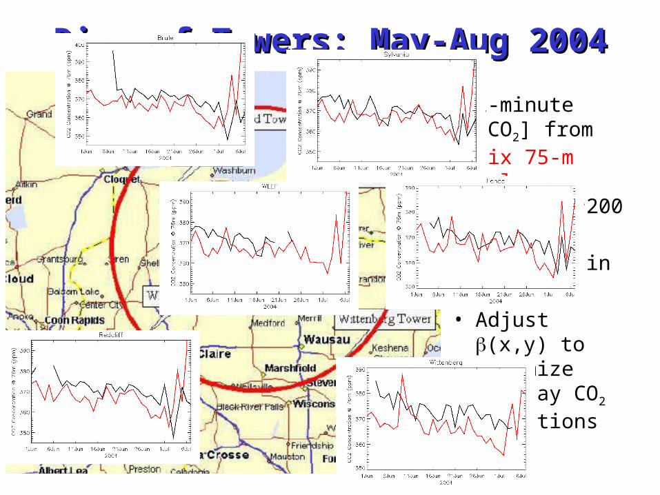
Ring of Towers: May-Aug 2004Ring of Towers: May-Aug 2004

• 1-minute [CO2] from six 75-m telecom towers, ~200 km radius

• Simulate in SiB-RAMS

• Adjust β(x,y) to optimize mid-day CO2 variations

Back-trajectory “Influence Back-trajectory “Influence Functions”Functions”

• Release imaginary “particles” every hour from each tower “receptor”

• Trace them backward in time, upstream, using flow fields saved from RAMS

• Count up where particles have been that reached receptor at each obs time

• Shows quantitatively how much each upstream grid cell contributed to observed CO2

• Partial derivative of CO2 at each tower and time with respect to fluxes at each grid cell and time

∂[CO2(t)]∂β (x,y)

QuickTime™ and aH.264 decompressor

are needed to see this picture.

31 Towers in 200731 Towers in 2007∂[CO2(t)]∂β (x,y)

Estimating the Estimating the ββ’s’s

• Full Kalman Filter (Bayesian synthesis)

• Maximum Likelihood Ensemble Filter (MLEF, Zupanski et al)

• Markov-Chain Monte Carlo (MCMC)• Problem is terribly underconstrained!• The science (art?) is in the

specification of covariance structures• Marek and Andrew will discuss …