forecast jumpiness: good or bad? - dtcenter.org · forecast jumpiness: good or bad? zoltan toth....

1

FORECAST JUMPINESS: GOOD OR BAD?

Zoltan Toth

Global Systems DivisionNOAA/OAR/ESRL

Ackn.: Yuejian Zhu, Malaquias Pena, Yuanfu Xie, and Olivier Talagrand (1)

(1) : Ecole Normale Superior and LMD, Paris, France

http://wwwt.emc.ncep.noaa.gov/gmb/ens/index.html

2

OUTLINE / SUMMARY• Definition of jumpiness

– Changes in forecast error• Magnitude• Pattern

• Forecaster’s desire– Small error– Low jumpiness

• NWP principles– Jumpiness increases in single forecast as error variance is decreased

• Solution– Ensemble forecasting

• Must be “jump-free”

• Measure of jumpiness– Time consistency histogram

• After analysis rank (Talagrand) histogram

• Cloud verification examples from Local Analysis and Prediction System (LAPS)– Interest in collaboration

3

BACKGROUND• NWP forecast error characteristics

– Originate from imperfect• Initial conditions• Numerical models

– Amplify due to chaotic dynamics

• Definition of forecast jumpiness– When successive forecasts for same verifying event (in time/space) look

different =>– Error in successive forecasts are different

• Either size or pattern of error

• Successive initial conditions may have errors different in – Size or – Patterns

• Some model errors may be systematic– Stable from one initial condition to next

• Jumpiness is not verification statistic– Diagnostic of a DA/forecast system

• Verification metrics traditionally focus on error variance only– Not error pattern

4

JUMPINESS & USERS• Objective of NWP development

– Reduce forecast error variance

• Reduced error variance equals to– Reduced jumpiness

• Measure of forecast jumpiness at a given level of error variance– How correlated error patterns are in successive forecasts verifying at

same time/space

• Preference of some/most/all (?) forecasters– NO JUMPINESS

• Users don’t like big changes in forecasts

• Limitation of single value forecasts– Represent only one scenario

• Does not convey forecast uncertainty

• Proper and only defendable format of forecasts– Probabilistic

• Practical solution - Ensembles

5

JUMPINESS & NWP

• Is jumpiness a good or bad diagnostic feature for NWP systems?

• Good observing and analysis system– Error in analysis should be uncorrelated to error in background forecast

=>• Low jumpiness is necessary condition for good observing/DA systems

– Not sufficient as low error variance is also a necessary condition

• Forecasters’ desire for low jumpiness contradicts NWP principles– Lowering error variance necessarily leads to increased jumpiness

• Goal is not to increase jumpiness, that’s an artifact of decreasing error variance– Removing temporally correlated errors from DA/forecast system

6

EXAMPLE OF GLOBAL NWP FORECASTSFORECAST ERROR VARIANCE

A

DC

B

Pena et al

7

CORRELATION BETWEEN ANALYSIS & FORECAST ERRORS

A

D

C

B

Pena et al

8

JUMPINESS & ENSEMBLE FORECASTS• Jumpiness is a virtue of single (control) NWP forecasts

– Is it true for ensembles?

• Ensembles designed to capture forecast uncertainty– Successive ensembles must convey reduced uncertainty

• Shorter range ensemble cloud must statistically lay within longer range cloud

• How to measure if an ensemble performs as it should?

• Method related to how we assess statistical consistency between ensemble and verifying analysis– Analysis Rank (or Talagrand) Histogram

• Measure temporal consistency in successive ensembles– Time consistency histogram

• Toth, Z., O. Talagrand, G. Candille, and Y. Zhu, 2002: Probability and ensemble forecasts (final draft). In: Environmental Forecast Verification: A practitioner's guide in atmospheric science. Ed.: I. T. Jolliffe and D. B. Stephenson. Wiley, pp.137-164.

• Role of analysis taken by members in succeeding ensemble

9

ANALYSIS RANK HISTOGRAM (TALAGRAND DIAGRAM)MEASURE OF RELIABILITY

EXAMPLE FOR 3 ENSEMBLES

10

• Canadian• Ensemble filter

• Low time consistency between successive perturbations

• Noise added to observations• ECMWF

• Singular vectors• Too low spread at short lead time• No time consistency between

successive perturbations

• NCEP• Ensemble Transform

• Strong time conistency• No noise added

• No model related perturbations

Zhu et al

11

OUTLINE / SUMMARY• Definition of jumpiness

– Changes in forecast error• Magnitude• Pattern

• Forecaster’s desire– Small error– Low jumpiness

• NWP principles– Jumpiness increases in single forecast as error variance is decreased

• Solution– Ensemble forecasting

• Must be “jump-free”

• Measure of jumpiness– Time consistency histogram

• After analysis rank (Talagrand) histogram

• Cloud verification examples from Local Analysis and Prediction System (LAPS)– Interest in collaboration

An Evaluation of Various WRF-ARW Microphysics Using Simulated GOES Imagery for an Atmospheric River Event

Affecting the California Coast

Isidora Jankov, Lewis D. Grasso, Manajit Sengupta, Paul J. Neiman, Dusanka Zupanski, Milija Zupanski, Daniel Lindsey, and Renate Brummer

Accepted for publication in JHM

o The main purpose of the present study was to assess value of synthetic satellite imagery as a tool to evaluate the performance of a model in addition to more traditional approaches.

o Use of synthetic imagery is a unique way to indirectly evaluate the performance of various microphysical schemes available within current models for NWP.

o For this purpose, synthetic GOES-10 imagery at 10.7 µm was produced using output from the WRF-ARW model.

o Simulation of an atmospheric river event that occurred on 30 December 2005 was performed.

MOTIVATION

EXPERIMENT DESIGNSIMULATIONS

• 24hr simulation starting 30 December 2005 at 12 UTC

• WRF-ARW 20km horizontal grid spacing mother domain with 5km grid spacing nest

• 5 different Microphysics Lin, WSM6, Thompson, Schultz and double moment Morrison

• YSU PBL

• LAPS analysis and 40 km Eta LBCs

Brightness temperatures observed from GOES-10 and simulated by model runs using Lin,

WSM6, Thompson, Schultz and 2-moment Morrison microphysics, valid on 31 December 2005 at 00 UTC.

Probability of occurrence histograms

Objective Skill Measures

POD, TS, FAR, Bias for 12-hour brightness temperature forecasts, valid at 00 UTC 30 December 2005, for the five different model solutions.

SUMMARY

o All of the evaluated microphysical schemes, except Lin, performed generally well in simulating high clouds, while the lower cloud coverage was somewhat underestimated, especially at earlier times.

o The Lin microphysics showed tendency to produce too many high clouds.

o Results suggest that synthetic satellite imagery can be very useful as a tool to evaluate the performance of a model.

o Further more, synthetic satellite imagery can be potentially useful in better understanding and improvement of the existing microphysical schemes

Verification by using simulated vs. observed reflectivity (NSF project cases)

Analysis6-hr Diabatically (LAPS) initialized

WRF-ARW forecast

13 June 2002

Jankov & Albers

Bias & ETS June 13 2002Jankov & Albers

16 June 2002

3-hr ForecastAnalysis

Jankov & Albers

Bias & ETS June 16 2002

0246

0 15 30 45 60 75 90 105 120 135 150 165

Bias

Forecast Minutes

Bias 20dBZ

LIN-Kessler

WSM6-Kessler

SCH-Kessler

0246

0 15 30 45 60 75 90 105 120 135 150 165

Bias

Forecast Minutes

Bias 30dBZ

LIN-Kessler

WSM6-Kessler

SCH-Kessler

0

5

10

0 15 30 45 60 75 90 105 120 135 150 165

Bias

Forecast Minutes

Bias 40dBZ

LIN-Kessler

WSM6-Kessler

SCH-Kessler

00.20.40.60.8

0 15 30 45 60 75 90 105 120 135 150 165

ETS

Forecast Minutes

ETS 20dBZ

LIN-Kessler

WSM6-Kessler

SCH-Kessler

00.20.40.6

0 15 30 45 60 75 90 105 120 135 150 165ET

SForecast Minutes

ETS 30dBZ

LIN-Kessler

WSM6-Kessler

SCH-Kessler

00.20.40.6

0 15 30 45 60 75 90 105 120 135 150 165

ETS

Forecvast Minutes

ETS 40dBZ

LIN-Kessler

WSM6-Kessler

SCH-Kessler

Jankov & Albers

Ongoing Long-wave-radiation(analysis and fcsts with observations overlaid)

Downward Solar Radiation Fcst. vs. Observations Albers et al

26

BACKGROUND

27

OUTLINE / SUMMARY• SCIENCE OF FORECASTING

– GOAL OF SCIENCE Forecasting– VERIFICATION Model development, user feedback

• GENERATION OF PROBABILISTIC FORECASTS– SINGLE FORECASTS Statistical rendition of pdf– ENSEMBLE FORECASTS NWP-based, case-dependent pdf

• ATTRIBUTES OF FORECAST SYSTEMS– RELIABILITY Forecasts look like nature statistically– RESOLUTION Forecasts indicate actual future developments

• VERIFICATION OF PROBABILSTIC & ENSEMBLE FORECASTS– UNIFIED PROBABILISTIC MEASURES Dimensionless– ENSEMBLE MEASURES Evaluate finite sample

• STATISTICAL POSTPROCESSING OF FORECASTS– STATISTICAL RELIABILITY Make it perfect– STATISTICAL RESOLUTION Keep it unchanged

28

SCIENCE OF FORECASTING • Ultimate goal of science

– Forecasting• Meteorology is in forefront

– Weather forecasting constantly in public’s eye

• Approach– Observe what is relevant and available

• Analyze data– Build general knowledge about nature based on analysis

• Generalization & abstraction – Laws, relationships– Build model of reality based on general knowledge

• Conceptual• Quantitative/numerical, including various physical etc processes• Analog

– Predict what’s not observable in• Space – eg, data assimilation• Time - eg, future weather• Variables / processes

– Verify (ie, compare with observations)• Determine to what extent model represents reality• Assess if predictions have any utility

– Improve general knowledge and model

29

PREDICTIONS IN TIME

• Method– Use model of nature for projection in time– Start model with estimate of state of nature at “initial” time

• Sources of errors– Discrepancy between model and nature

• Added at every time step– Discrepancy between estimated and actual state of nature

• Initial error

• Chaotic systems– Common type of dynamical systems

• Characterized with at least one perturbation pattern that amplifies– All errors project onto amplifying directions

• Any initial and/or model error– Predictability limited

• Ed Lorenz’ legacy• Verification quantifies situation

30

MOTIVATION FOR ENSEMBLE FORECASTING• FORECASTS ARE NOT PERFECT - IMPLICATIONS FOR:

– USERS:• Need to know how often / by how much forecasts fail• Economically optimal behavior depends on

– Forecast error characteristics– User specific application

» Cost of weather related adaptive action» Expected loss if no action taken

– EXAMPLE: Protect or not your crop against possible frostCost = 10k, Potential Loss = 100k => Will protect if P(frost) > Cost/Loss=0.1• NEED FOR PROBABILISTIC FORECAST INFORMATION

– DEVELOPERS:• Need to improve performance - Reduce error in estimate of first moment

– Traditional NWP activities (I.e., model, data assimilation development)• Need to account for uncertainty - Estimate higher moments

– New aspect – How to do this?• Forecast is incomplete without information on forecast uncertainty • NEED TO USE PROBABILISTIC FORECAST FORMAT

31

GENERATION OF PROBABILISTIC FORECASTS

• How to determine forecast probability?– Fully statistical methods – losing relevance– Numerical modeling

• Liouville Equations provide pdf’s– Not practical (computationally intractable)

• Finite sample of pdf– Single or multiple (ensemble) integrations

» Increasingly finer resolution estimate in probabilities

• How to make (probabilistic) forecasts reliable?– Construct pdf

• Assess reliability– Construct frequency distribution of observations following forecast

classes• Replace form of forecast with associated frequency distribution of

observations– Production and verification of forecasts connected in operations

32

FORECASTING IN A CHAOTIC ENVIRONMENT –PROBABILISTIC FORECASTING BASED ON A SINGLE FORECAST –

One integration with an NWP model, combined with past verification statisticsDETERMINISTIC APPROACH - PROBABILISTIC FORMAT

•Does not contain all forecast information

•Not best estimate for future evolution of system

•UNCERTAINTY CAPTURED IN TIME AVERAGE SENSE -

•NO ESTIMATE OF CASE DEPENDENT VARIATIONS IN FCST UNCERTAINTY

33

SCIENTIFIC BACKGROUND:WEATHER FORECASTS ARE UNCERTAIN

Buizza 2002

34

FORECASTING IN A CHAOTIC ENVIRONMENT - 2DETERMINISTIC APPROACH - PROBABILISTIC FORMAT

PROBABILISTIC FORECASTING -Based on Liuville Equations

Continuity equation for probabilities, given dynamical eqs. of motion

• Initialize with probability distribution function (pdf) at analysis time• Dynamical forecast of pdf based on conservation of probability values• Prohibitively expensive -

• Very high dimensional problem (state space x probability space)• Separate integration for each lead time• Closure problems when simplified solution sought

35

FORECASTING IN A CHAOTIC ENVIRONMENT - 3DETERMINISTIC APPROACH - PROBABILISTIC FORMAT

MONTE CARLO APPROACH – ENSEMBLE FORECASTING

• IDEA: Sample sources of forecast error• Generate initial ensemble perturbations• Represent model related uncertainty

• PRACTICE: Run multiple NWP model integrations• Advantage of perfect parallelization• Use lower spatial resolution if short on resources

• USAGE: Construct forecast pdf based on finite sample• Ready to be used in real world applications• Verification of forecasts• Statistical post-processing (remove bias in 1st, 2nd, higher moments)

CAPTURES FLOW DEPENDENT VARIATIONSIN FORECAST UNCERTAINTY

36

T00Z

80m

6hrs

T06Z

80m

T12Z

80m

T18Z

80m

Up to 16-d

Up to 16-d

Up to 16-d

Up to 16-d

Re-scaling

Re-scaling

Re-scaling

Re-scaling

6 hours ET / breeding cycle

Next T00Z

37

USER REQUIREMENTS:PROBABILISTIC FORECAST INFORMATION IS CRITICAL

38

USER REQUIREMENTS• General characteristics of forecast users

– Each user affected in specific way by• Various weather elements at • Different points in time & • Space

• Requirements for optimal decisions related to operations affected by weather– Possible weather scenarios with covariances across

• Variables, space, and time

• Provision of weather information– Specific information needed by each user can’t be foreseen or provided

• Only vanilla-type often used probabilistic info can be distributed– Ensemble data must be made accessible to users in statistically reliable form

• All forecast info can be derived from this, including vanilla probabilistic products

• IT infrastructure requirements– Staging ground for ensemble data (disc)– Sophisticated data access / interrogation tools

• Subset ensemble data, derive required parameters– Technical achievements - NOMADS, AWIPS2

– Telecommunication (bandwidth)

39

AVIATION EXAMPLE• Recovery of a carrier from weather related

disruptions– Operational decisions depend on multitude of

factors• Based on United / Hemispheres March 2009 article, p.

11-12

• Factors affecting operations– Weather

• Over large region / CONUS during coming few days– Federal regulations / aircraft limitations

• Dispatchers / load planners– Aircraft availability

• Scheduling / flight planning– Maintenance

• Pre-location of spare parts & other assets where neededRti

40

SELECTION OF OPTIMAL USER PROCEDURES• Generate ensemble weather scenarios ei, i = 1,

n• Assume weather is ei, define optimal operation

procedures oi• Assess cost/loss cij using oi over all weather

scenarios ej• Select oi with minimum expected (mean)

cost/loss ci over e1,…en as optimum operation

COST/LOSS cijGIVEN ej

WEATHER & oiOPERATIONS

ENSEMBLE SCENARIOS

e1 e2 . en

o1 c11 c12 . cn c1

o2 c21 c22 . c2n c2

. . . . . .

on cn1 cn2 . cnn cn

OP

ER

ATIO

NP

RO

CE

DU

RE

S

EXP

EC

TED

CO

ST

41

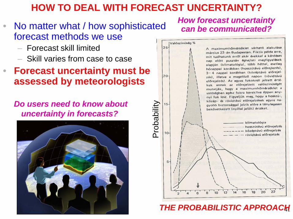
• No matter what / how sophisticated forecast methods we use– Forecast skill limited– Skill varies from case to case

• Forecast uncertainty must be assessed by meteorologists

Do users need to know about uncertainty in forecasts?

HOW TO DEAL WITH FORECAST UNCERTAINTY?How forecast uncertainty can be communicated?

Prob

abilit

y

THE PROBABILISTIC APPROACH

42

Weeks

Type

of G

uida

nce

Warnings & Alert Coordination

Watches

Forecasts

Threat Assessments

Guidance

Outlook

Minutes DaysHours Years

Lead Time

SeasonsMonths

Forecast Uncertainty

Protection of Life/Property

Flood mitigationNavigation

TransportationFire weather

HydropowerAgriculture

EcosystemHealth

CommerceEnergy

SOCIO-ECONOMIC BENEFITS OFSEAMLESS WEATHER/CLIMATE FORECAST SUITE

Reservoir controlRecreation

43

ENSEMBLE FORECASTS

• Definition– Finite sample to estimate full probability distribution

• Full solution (Liouville Eqs.) computationally intractable

• Interpretation (assignment of probabilities)– Crude

• Step-wise increase in cumulative forecast probability distribution– Performance dependent on size of ensemble

– Enhanced• Inter- & extrapolation (dressing)

– Performance improvement depends on quality of inter- & extrapolation» Based on assumptions

Linear interpolation (each member equally likely)» Based on verification statistics

Kernel or other methods (Inclusion of some statist. bias-correction)

46

144 hr forecast

Verification

Poorly predictable large scale waveEastern Pacific – Western US

Highly predictable small scale waveEastern US

50

FORECAST EVALUATION • Statistical approach

– Evaluates set of forecasts and not a single forecast• Interest in comparing forecast systems

– Forecasts generated by same procedure– Sample size affects how fine stratification is possible

• Level of details is limited– Size of sample limited by available obs. record (even for hind-casts)

• Statistical significance in comparative verification– Error in proxy for truth

• Observations or numerical analysis

• Types– Forecast statistics

• Depends only on forecast properties– Verification statistics

• Comparison of forecast and proxy for “truth” in statistical sense– Depends on both natural and forecast systems– Nature represented by “proxy”

» Observations (including observational error)» Numerical analysis (including analysis error)

51

FORECAST VERIFICATION

• Types– Measures of quality

• Environmental science issues– Main focus here

– Measures of utility• Multidisciplinary

– Social & economic issues, beyond environmental sciences– Socio-economic value of forecasts is ultimate measure

» Approximate measures can be constructed

• Quality vs. utility– Improved quality

• Generally permits enhanced utility (assumption)– How to improve utility if quality is fixed?

• Providers communicate all available information– E.g., offer probabilistic or other information on forecast uncertainty

» Engage in education, training• Users identify forecast aspects important to them

– Can providers selectively improve certain aspects of forecasts?» E.g, improve precipitation forecasts without improving circulation forecasts?

52

EVALUATING QUALITY OF FORECAST SYSTEMS

• Goal– Infer comparative information about forecast systems

• Value added by– New methods– Subsequent steps in end-to-end forecast process (eg., manual changes)

• Critical for monitoring and improving operational forecast systems

• Attributes of forecast systems– Traditionally, forecast attributes defined separately for each fcst format– General definition needed

• Need to compare forecasts – From any system &– Of any type / format

» Single, ensemble, categorical, probabilistic, etc• Supports systematic evaluation of

– End-to-end (provider-user) forecast process» Statistical post-processing as integral part of system

53

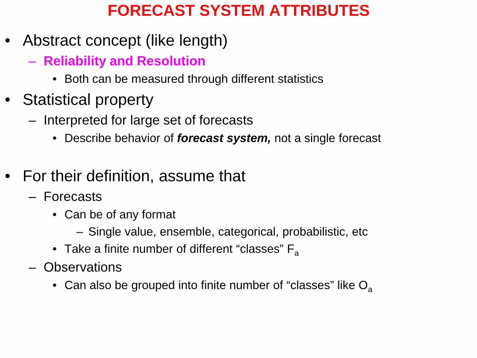
FORECAST SYSTEM ATTRIBUTES

• Abstract concept (like length)– Reliability and Resolution

• Both can be measured through different statistics

• Statistical property– Interpreted for large set of forecasts

• Describe behavior of forecast system, not a single forecast

• For their definition, assume that– Forecasts

• Can be of any format– Single value, ensemble, categorical, probabilistic, etc

• Take a finite number of different “classes” Fa

– Observations• Can also be grouped into finite number of “classes” like Oa

54

STATISTICAL RELIABILITY – TEMPORAL AGGREGATESTATISTICAL CONSISTENCY OF FORECASTS WITH OBSERVATIONS

BACKGROUND:• Consider particular forecast class – Fa• Consider frequency distribution of observations that follow forecasts Fa - fdoa

DEFINITION:• If forecast Fa has the exact same form as fdoa, for all forecast classes,

the forecast system is statistically consistent with observations =>The forecast system is perfectly reliable

MEASURES OF RELIABILITY:• Based on different ways of comparing Fa and fdoa

EXAMPLES:CONTROL FCST ENSEMBLE

55

STATISTICAL RESOLUTION – TEMPORAL EVOLUTIONABILITY TO DISTINGUISH, AHEAD OF TIME, AMONG DIFFERENT OUTCOMES

BACKGROUND:• Assume observed events are classified into finite number of classes, like OaDEFINITION:• If all observed classes (Oa, Ob,…) are preceded by

– Distinctly different forecasts (Fa, Fb,…)– The forecast system “resolves” the problem =>

The forecast system has perfect resolutionMEASURES OF RESOLUTION:• Based on degree of separation of fdo’s that follow various forecast classes • Measured by difference between fdo’s & climate distribution• Measures differ by how differences between distributions are quantified

FORECASTS OBSERVATIONSEXAMPLES

56

CHARACTERISTICS OF RELIABILITY & RESOLUTION• Reliability

– Related to form of forecast, not forecast content• Fidelity of forecast

– Reproduce nature when resolution is perfect, forecast looks like nature– Not related to time sequence of forecast/observed systems– How to improve?

• Make model more realistic– Also expected to improve resolution

• Statistical bias correction: Can be statistically imposed at one time level – If both natural & forecast systems are stationary in time &– If there is a large enough set of observed-forecast pairs– Link with verification:

» Replace forecast with corresponding fdo

• Resolution – Related to inherent predictive value of forecast system– Not related to form of forecasts

• Statistical consistency at one time level (reliability) is irrelevant– How to improve?

• Enhanced knowledge about time sequence of events– More realistic numerical model should help

» May also improve reliability

57

CHARACTERISTICS OF FORECAST SYSTEM ATTRIBUTES

RELIABILITY AND RESOLUTION ARE

• General forecast attributes– Valid for any forecast format (single, categorical, probabilistic, etc)

• Independent attributes– For example

• Climate pdf forecast is perfectly reliable, yet has no resolution• Reversed rain / no-rain forecast can have perfect resolution and no reliability

– To separate them, they must be measured according to general definition• If measured according to traditional, narrower definition

– Reliability & resolution can be mixed

• Function of forecast quality– There is no other relevant forecast attribute

• Perfect reliability and perfect resolution = perfect forecast system =– “Deterministic” forecast system that is always correct

• Both needed for utility of forecast systems– Need both reliability and resolution

• Especially if no observed/forecast pairs available (eg, extreme forecasts, etc)

58

FORMAT OF FORECASTS – PROBABILSITIC FORMAT

• Do we have a choice?– When forecasts are imperfect

• Only probabilistic format can be reliable/consistent with nature

• Abstract concept – Related to forecast system attributes

• Space of probability – dimensionless pdf or similar format– For environmental variables (not those variables themselves)

• Definition1. Define event

• Function of concrete variables, features, etc– E.g., “temperature above freezing”; “thunderstorm”

2. Determine probability of event occurring in future– Based on knowledge of initial state and evolution of system

59

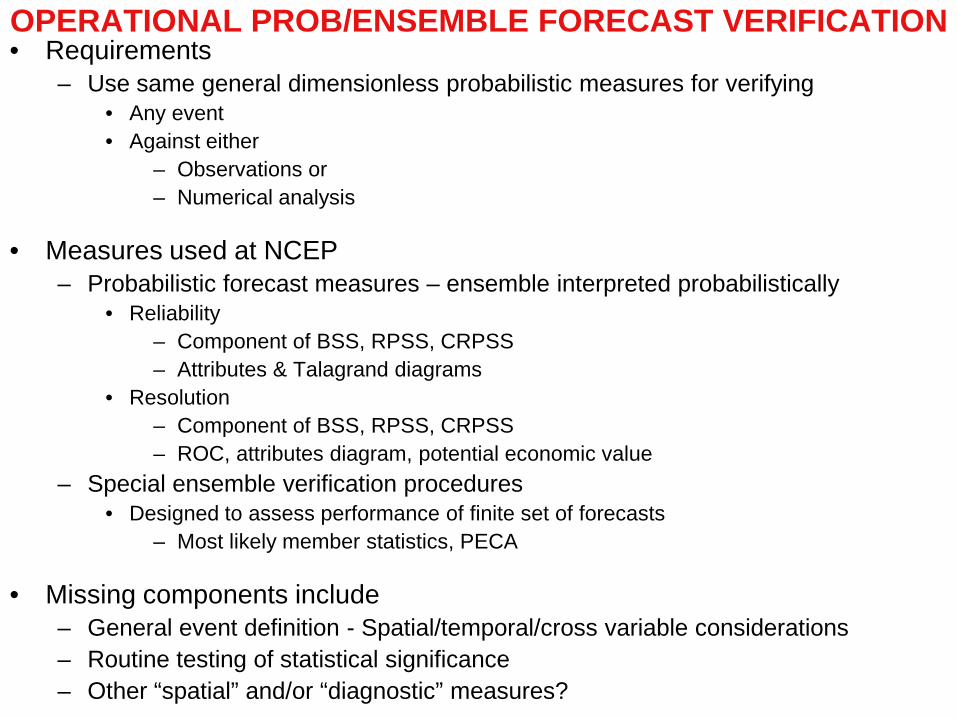
OPERATIONAL PROB/ENSEMBLE FORECAST VERIFICATION• Requirements

– Use same general dimensionless probabilistic measures for verifying• Any event• Against either

– Observations or– Numerical analysis

• Measures used at NCEP– Probabilistic forecast measures – ensemble interpreted probabilistically

• Reliability– Component of BSS, RPSS, CRPSS– Attributes & Talagrand diagrams

• Resolution– Component of BSS, RPSS, CRPSS– ROC, attributes diagram, potential economic value

– Special ensemble verification procedures• Designed to assess performance of finite set of forecasts

– Most likely member statistics, PECA

• Missing components include– General event definition - Spatial/temporal/cross variable considerations– Routine testing of statistical significance– Other “spatial” and/or “diagnostic” measures?

60

FORECAST PERFORMANCE MEASURES

MEASURES OF RELIABILITY:DESCRIPTION:Statistically compares any sample of forecasts with sample of corresponding observations

GOAL:To assess similarity of samples (e.g., whether 1st and 2nd moments match)EXAMPLES:Reliability component of

Brier ScoreRanked Probability Score

Analysis Rank HistogramSpread vs. Ens. Mean errorEtc.

MEASURES OF RESOLUTION:DESCRIPTION:Compares the distribution of observations that follows different classes of forecasts with the climate distribution (as reference)GOAL:To assess how well the observations are separated when grouped by different classes of preceding fcstsEXAMPLES:Resolution component of

Brier ScoreRanked Probability Score

Information contentRelative Operational CharacteristicsRelative Economic ValueEtc.

COMMON CHARACTERISTIC: Function of both forecast and observed values

COMBINED (REL+RES) MEASURES: Brier, Cont. Ranked Prob. Scores, rmse, PAC,…

61

EXAMPLE – PROBABILISTIC FORECASTS

RELIABILITY:Forecast probabilities for given event

match observed frequencies of thatevent (with given prob. fcst)

RESOLUTION:Many forecasts fall into classes

corresponding to high or lowobserved frequency of given event

(Occurrence and non-occurrence ofevent is well resolved by fcstsystem)

63

PROBABILISTIC FORECAST PERFORMANCE MEASURESTO ASSESS TWO MAIN ATTRIBUTES OF PROBABILISTIC FORECASTS:

RELIABILITY AND RESOLUTIONUnivariate measures: Statistics accumulated point by point in spaceMultivariate measures: Spatial covariance is considered

BRIER SKILL SCORE (BSS)COMBINED MEASURE OF RELIABILITY AND RESOLUTION

EXAMPLE:

64

BRIER SKILL SCORE (BSS)

METHOD:Compares pdf against analysis • Resolution (random error)• Reliability (systematic error)

EVALUATIONBSS Higher betterResolution Higher betterReliability Lower better

RESULTSResolution dominates initiallyReliability becomes important later• ECMWF best throughout

– Good analysis/model?• NCEP good days 1-2

– Good initial perturbations?– No model perturb. hurts later?

• CANADIAN good days 8-10– Model diversity helps?

May-June-July 2002 average Brier skill score for the EC-EPS (grey lines with fullcircles), the MSC-EPS (black lines with open circles) and the NCEP-EPS (black lineswith crosses). Bottom: resolution (dotted) and reliability(solid) contributions to theBrier skill score. Values refer to the 500 hPa geopotential height over the northernhemisphere latitudinal band 20º-80ºN, and have been computed considering 10equally-climatologically-likely intervals (from Buizza, Houtekamer, Toth et al, 2004)

COMBINED MEASURE OF RELIABILITY AND RESOLUTION

65

BRIER SKILL SCORECOMBINED MEASURE OF RELIABILITY AND RESOLUTION

66

RANKED PROBABILITY SCORECOMBINED MEASURE OF RELIABILITY AND RESOLUTION

67

0%

100%

50%

p07 p09p08p06p03p02p01 p04 p05 p10

Obs (truth)

∫+∞

∞−

−−= dxxxHxFCRPS 20 )]()([

Continuous Rank Probability Score

X

Xo

Heaviside Function H

{ )(0)(10 )( o

o

xxxxxxH ≤

>=−

Order of 10 ensemble members (p01, p02,…,p10)

c

fc

CRPSCRPSCRPSCRPSS −=CRP Skill Score is

68

ANALYSIS RANK HISTOGRAM (TALAGRAND DIAGRAM)MEASURE OF RELIABILITY

69

ENSEMBLE MEAN ERROR VS. ENSEMBLE SPREAD

Statistical consistency between the ensemble and the verifying analysis means that the verifying analysis should be statistically indistinguishable from the ensemble members =>

Ensemble mean error (distance between ens. mean and analysis) should be equal to ensemble spread (distance between ensemble mean and ensemble members)

MEASURE OF RELIABILITY

In case of a statistically consistent ensemble, ens. spread = ens. mean error,and they are both a MEASURE OF RESOLUTION. In the presence of bias, both rms error and PAC will be a combined measure of reliability and resolution

70

INFORMATION CONTENTMEASURE OF RESOLUTION

71

RELATIVE OPERATING CHARACTERISTICSMEASURE OF RESOLUTION

72

ECONOMIC VALUE OF FORECASTSMEASURE OF RESOLUTION

73

PERTURBATION VS. ERROR CORRELATION ANALYSIS (PECA)

METHOD: Compute correlation between ens perturbtns and error in control fcst for

– Individual members– Optimal combination of members– Each ensemble – Various areas, all lead time

EVALUATION: Large correlation indicates ens captures error in control forecast

– Caveat – errors defined by analysisRESULTS:

– Canadian best on large scales• Benefit of model diversity?

– ECMWF gains most from combinations• Benefit of orthogonalization?

– NCEP best on small scale, short term• Benefit of breeding (best estimate initial

error)?– PECA increases with lead time

• Lyapunov convergence• Nonlilnear saturation

– Higher values on small scales

MULTIVATIATE COMBINED MEASURE OFRELIABILITY & RESOLUTION

74

WHAT WE NEED FOR POSTPROCESSING TO WORK?

• LARGE SET OF FCST – OBS PAIRS• Consistency defined over large sample – need same for post-processing• Larger the sample, more detailed corrections can be made

• BOTH FCST AND REAL SYSTEMS MUST BE STATIONARY IN TIME• Otherwise can make things worse• Subjective forecasts difficult to calibrate

HOW WE MEASURE STATISTICAL INCONSISTENCY?

• MEASURES OF STATIST. RELIABILITY • Time mean error• Analysis rank histogram (Talagrand diagram)• Reliability component of Brier etc scores• Reliability diagram

75

SOURCES OF STATISTICAL INCONSISTENCY• TOO FEW FORECAST MEMBERS

• Single forecast – inconsistent by definition, unless perfect• MOS fcst hedged toward climatology as fcst skill is lost

• Small ensemble – sampling error due to limited ensemble size(Houtekamer 1994?)

• MODEL ERROR (BIAS)• Deficiencies due to various problems in NWP models

• Effect is exacerbated with increasing lead time

• SYSTEMATIC ERRORS (BIAS) IN ANALYSIS• Induced by observations

• Effect dies out with increasing lead time• Model related

• Bias manifests itself even in initial conditions

• ENSEMBLE FORMATION (INPROPER SPREAD)• Not appropriate initial spread• Lack of representation of model related uncertainty in ensemble

• I. E., use of simplified model that is not able to account for model related uncertainty

76

HOW TO IMPROVE STATISTICAL CONSISTENCY?

• MITIGATE SOURCES OF INCONSISTENCY • TOO FEW MEMBERS

• Run large ensemble• MODEL ERRORS

• Make models more realistic• INSUFFICIENT ENSEMBLE SPREAD

• Enhance models so they can represent model related forecast uncertainty

• OTHERWISE =>

• STATISTICALLY ADJUST FCST TO REDUCE INCONSISTENCY• Unpreferred way of doing it• What we learn can feed back into development to mitigate problem at sources• Can have LARGE impact on (inexperienced) users• Two separate issues

• Bias correct against NWP analysis• Reduce lead time dependent model behavior

• Downscale NWP analysis• Connect with observed variables that are unresolved by NWP models

78

OUTLINE / SUMMARY• SCIENCE OF FORECASTING

– GOAL OF SCIENCE Forecasting– VERIFICATION Model development, user feedback

• GENERATION OF PROBABILISTIC FORECASTS– SINGLE FORECASTS Statistical rendition of pdf– ENSEMBLE FORECASTS NWP-based, case-dependent pdf

• ATTRIBUTES OF FORECAST SYSTEMS– RELIABILITY Forecasts look like nature statistically– RESOLUTION Forecasts indicate actual future developments

• VERIFICATION OF PROBABILSTIC & ENSEMBLE FORECASTS– UNIFIED PROBABILISTIC MEASURES Dimensionless– ENSEMBLE MEASURES Evaluate finite sample

• STATISTICAL POSTPROCESSING OF FORECASTS– STATISTICAL RELIABILITY Make it perfect– STATISTICAL RESOLUTION Keep it unchanged

79

http://wwwt.emc.ncep.noaa.gov/gmb/ens/ens_info.htmlToth, Z., O. Talagrand, and Y. Zhu, 2005: The Attributes of Forecast Systems: A Framework for the Evaluation and Calibration ofWeather Forecasts. In: Predictability Seminars, 9-13 September 2002, Ed.: T. Palmer, ECMWF, pp. 584-595. Toth, Z., O. Talagrand, G. Candille, and Y. Zhu, 2003: Probability and ensemble forecasts. In: Environmental Forecast Verification: A practitioner's guide in atmospheric science. Ed.: I. T. Jolliffe and D. B. Stephenson. Wiley, p. 137-164.

80

BACKGROUND

81

NOTES FOR NEXT YEAR

• Define predictand– Exhaustive set of events, eg

• Continuous temperature• Precipitation type (Categorical)

82

SUMMARY• WHY DO WE NEED PROBABILISTIC FORECASTS?

– Isn’t the atmosphere deterministic? YES, but it’s also CHAOTICFORECASTER’S PERSPECTIVE USER’S PERSPECTIVEEnsemble techniques Probabilistic description

• WHAT ARE THE MAIN ATTRIBUTES OF FORECAST SYSTEMS?– RELIABILITY Stat. consistency with distribution of corresponding observations– RESOLUTION Different events are preceded by different forecasts

• WHAT ARE THE MAIN TYPES OF FORECAST METHODS?– EMPIRICAL Good reliability, limited resolution (problems in “new” situations)– THEORETICAL Potentially high resolution, prone to inconsistency

• ENSEMBLE METHODS– Only practical way of capturing fluctuations in forecast uncertainty due to

• Case dependent dynamics acting on errors in– Initial conditions– Forecast methods

• HOW CAN PROBABILSTIC FORECAST PERFORMANCE BE MEASURED?Various measures of reliability and resolution

• STATISTICAL POSTPROCESSING Based on verification statistics – reduce statistical inconsistencies

83

OUTLINE

• STATISTICAL EVALUATION OF FORECAST SYSTEMS– ATTRIBUTES OF FORECAST SYSTEMS

• FORECAST METHODS– EMPIRICALLY BASED– THEORETICALLY BASED

• LIMITS OF PREDICTABILITY– LIMITING FACTORS– ASSESSING PREDICTABILITY

• Ensemble forecasting

• VERIFICATION MEASURES– MEASURING FORECAST SYSTEM ATTRIBUTES

• STATISTICAL POST-PROCESSING OF FORECASTS– IMPROVING STATISTICAL RELIABILITY

84

CRPS Decomposition

Yuejian Zhu

Environmental Modeling CenterNOAA/NWS/NCEP

Acknowledgements: Zoltan Toth EMC

85

0%

100%

50%

p07 p09p08p06p03p02p01 p04 p05 p10

Obs (truth)

∫+∞

∞−


Continuous Rank Probability Score

X

Xo

Heaviside Function H

{ )(0)(10 )( o

o

xxxxxxH ≤

>=−


c

fc

CRPSCRPSCRPSCRPSS −=CRP Skill Score is

86

0%

100%

50%

p07 p09p08p06p03p02p01 p04 p05 p10

OBS (truth)

∫+∞

∞−


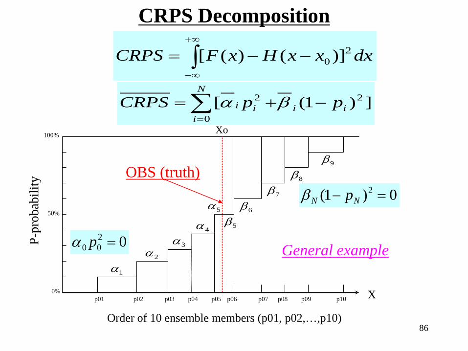
CRPS Decomposition

X

Xo


])1([ 2

0

2ii

N

iii ppCRPS −+=∑

=

βα

1α

3α2α

5α

4α 5β6β

7β8β

9β

P-pr

obab

ility

0200 =pα

0)1( 2 =− NN pβ

General example

87

0%

100%

50%

p07 p09p08p06p03p02p01 p04 p05 p10

OBS (truth)

CRPS Decomposition

X

Xo


])1([ 2

0

2ii

N

iii ppCRPS −+=∑

=

βα

1α

3α2α

5α

4α

6α7α

8α9α

P-pr

obab

ility

0200 =pα

10αExample of outlier (right)

88

0%

100%

50%

p07 p09p08p06p03p02p01 p04 p05 p10

OBS (truth)

CRPS Decomposition

X

Xo


])1([ 2

0

2ii

N

iii ppCRPS −+=∑

=

βα

1β

3β2β

4β5β

6β7β

8β9β

P-pr

obab

ility

0)1( 2 =− NN pβ

0β

Example of outlier (left)

89

CRPS Decomposition

])1([ 2

0

2ii

N

iii ppCRPS −+=∑

=

βα

∑=

−=N

iiii pogRELI

0

2)(

∑=

−+−=N

iiiiii popogCRPS

0

22 ])1()1[(

URESORELICRPS +−=

∑=

=N

iii ogRESO

0

2 ∑=

=N

iii ogU

0

ii

iio

βαβ+

=iiig βα +=Where:

90

0%

100%

50%

p07 p09p08p06p03p02p01 p04 p05 p10

CRPS Decomposition

X


])1([ 2

0

2ii

N

iii ppCRPS −+=∑

=

βα

1α

3α

2α

5α

4α

5β

6β7β

8β9β

P-pr

obab

ility

0200 =pα

0)1( 2 =− NN pβ

General example

8α

7α

6α

9α

1β2β

3β4β

ii

iio

βαβ+

=

ip

io

CDF of

CDF of

Observation frequency

Time, space average

91

CRPS Decomposition

0 10 20 30 40 50 60 70 80 90 100

Forecast probability (%)

Obs

erve

d re

lativ

e fr

eque

ncy

(%)

0

10

20

30

40

50

60

70

80

90

100

1g

3g

2g

5g

4g

7g

6g

9g

8g

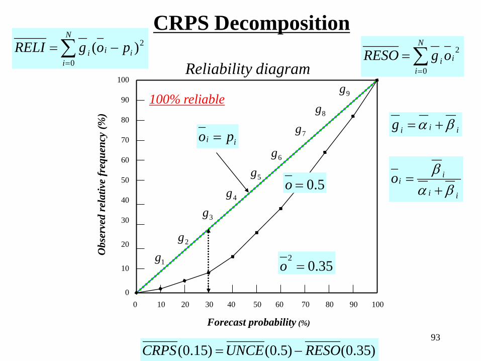
Reliability diagram

iiig βα +=∑=

−=N

iiii pogRELI

0

2)(

ii op −

io∑=

=N

iii ogRESO

0

2

ii

iio

βαβ+

=

92

CRPS Decomposition

0 10 20 30 40 50 60 70 80 90 100


Obs

erve

d re

lativ

e fr

eque

ncy

(%)

0

10

20

30

40

50

60

70

80

90

100

1g

3g

2g

5g

4g

7g

6g

9g

8g

Reliability diagram

iiig βα +=

∑=

−=N

iiii pogRELI

0

2)(

ii op −

0=io

∑=

=N

iii ogRESO

0

2

ii

iio

βαβ+

=

1=io Left outlier

Right outlier

RELICRPS =

100% unreliable

93

CRPS Decomposition

0 10 20 30 40 50 60 70 80 90 100


Obs

erve

d re

lativ

e fr

eque

ncy

(%)

0

10

20

30

40

50

60

70

80

90

100

1g

3g

2g

5g

4g

7g

6g

9g

8g

Reliability diagram

iiig βα +=

∑=

−=N

iiii pogRELI

0

2)( ∑=

=N

iii ogRESO

0

2

ii

iio

βαβ+

=

ii po =

100% reliable

35.02=o

5.0=o

)35.0()5.0()15.0( RESOUNCECRPS −=

94

CRPS Decomposition

CRPS : 0 ---------------- 1.0

RELI: 0 --------------- 0.5

RESO: 0 ---------------- 1.0

UNCE: 0 ---------------- 1.0

95

Ranked Probabilistic ScoreRanked (ordered) Probability Score (RPS) is to verify multi-category probability forecasts, to measure both reliability and resolution which based on climatologically equally likely bins

−

−−= ∑∑ ∑

== =

i

nn

k

i

i

nn OP

kRPS

1

2

1 1)(

111

c

cf

RPSRPSRPS

RPSS−

−=

1and

x

Verify AnalysisEnsemble Forecast

OBS On

FCST PROB Pn

0 00 01 00 00 0

0% 20%10% 0%10%30% 20% 0%0%10%

i=1

i=2

i=3

i=4

i=5

i=6

i=7

i=8

i=9

i=10 = k : number of categories

2)0.00.0( −

2)0.03.0( −

2)0.01.0( −

2)0.19.0( −

2)0.16.0( −

2)0.19.0( −

2)0.17.0( −

2)0.10.1( −

2)0.10.1( −

2)0.10.1( −

2

11)( ∑∑

==

−i

nn

i

nn OP

Example of 10 climatologically equally likely bins, 10 ensembles

96

RMSE and Spread Mean and absolute errors

CRPSS

10 meter wind (u-component)

Less biased,

There is less room to improve the skill by bias-correction only

97

RPSS .vs CRPSS

ROC score

Winter 2006-2007

NH 2m temperature

For

NCEP raw forecast (black)

NCEP bias corrected forecast (red)

NAEFS forecast (pink)

24h improvement by NAEFS

98

Brier Score (and decomposition)

1. BS (Brier Score)

∑=

−=n

kkk oy

nBS

1

2)(1

ref

f

refperf

reff

BSBS

BSBSBSBS

BSS −=−

−= 1

Where y is a forecast probability and o is an observation (probability), index k denotes a number of the n forecast event/pairs. y and o are limited from 0 to 1 in the probability sense. BS=0 is a perfect forecast, and BS=1 is missing everything

ref is the reference which is mostly climatology, BSperf=0 for perfect forecast, BSS is ranged from 0-1.

2. BSS (Brier Skill Score)

See <<Statistical Methods in the Atmospheric Science>> by D. S. Wilks, Chapter 7: Forecast Verification

Resolution – Reliability

Uncertainty=

99

Brier Score (and decomposition)3. Algebraic Decomposition of the Brier Score

After some algebra, the Brier Score can be expressed as three separated terms

∑∑==

−+−−−=I

iii

I

iiki ooooN

noyN

nBS

1

2

1

2 )1()(1)(1

∑∈

==iNk

ki

ii oN

yopo 1)|( 1

Reliability Resolution Uncertainty

Conditional probability of observed and sample climatology

∑=

=I

iiNn

1where

∑=

=n

kko

no

1

1and

100

Brier Score (and decomposition)4. Example for BS calculation

Ens(1) Ens(2) Ens(3) Ens(4) Ens(5) anlPoint 1 25 23 20 24 28 23Point 2 21 23 30 25 20 28Point 3 27 20 28 19 19 27Point 4 29 27 31 29 27 28Point 5 20 26 18 20 21 19

BinsC b< 22

F A22<= Cn <26

F ACa>=26

F APoint 1 0.2 0.0 0.6 1.0 0.2 0.0Point 2 0.4 0.0 0.4 0.0 0.2 1.0Point 3 0.6 0.0 0.0 0.0 0.4 1.0Point 4 0.0 0.0 0.0 0.0 1.0 1.0Point 5 0.8 1.0 0.0 0.0 0.2 0.0

Summary 0.120 0.064 0.216

The average Brier Score is 0.133 for this case, BS=0.133 (range from 0 to 1)

By considering three equally likely bins: Cb<22, 22<=Cn<26 and Ca>26

101

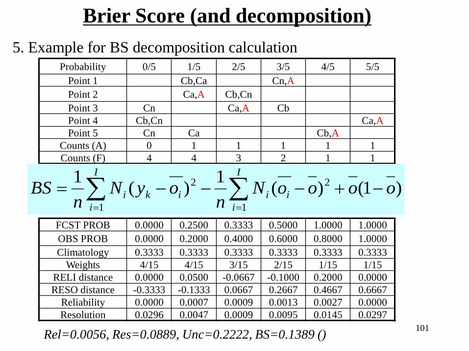
Brier Score (and decomposition)5. Example for BS decomposition calculation

Probability 0/5 1/5 2/5 3/5 4/5 5/5Point 1 Cb,Ca Cn,APoint 2 Ca,A Cb,CnPoint 3 Cn Ca,A CbPoint 4 Cb,Cn Ca,APoint 5 Cn Ca Cb,A

Counts (A) 0 1 1 1 1 1Counts (F) 4 4 3 2 1 1

FCST PROB 0.0000 0.2500 0.3333 0.5000 1.0000 1.0000OBS PROB 0.0000 0.2000 0.4000 0.6000 0.8000 1.0000Climatology 0.3333 0.3333 0.3333 0.3333 0.3333 0.3333

Weights 4/15 4/15 3/15 2/15 1/15 1/15RELI distance 0.0000 0.0500 -0.0667 -0.1000 0.2000 0.0000RESO distance -0.3333 -0.1333 0.0667 0.2667 0.4667 0.6667

Reliability 0.0000 0.0007 0.0009 0.0013 0.0027 0.0000Resolution 0.0296 0.0047 0.0009 0.0095 0.0145 0.0297

Rel=0.0056, Res=0.0889, Unc=0.2222, BS=0.1389 ()

∑∑==

−+−−−=I

iii

I

iiki ooooN

noyN

nBS

1

2

1

2 )1()(1)(1

102

Prob. Evaluation (multi-categories)4. Reliability and possible calibration ( remove bias ):

For period precipitation evaluation

Calibrated forecast

Raw forecast

Skill line

Resolution line

Climatological prob.

Obs

erve

d Fr

eque

ncy

(%)

0.16

forecast jumpiness: good or bad? - dtcenter.org · forecast jumpiness: good or bad? zoltan toth....

Documents