formworks-plus: improved pre-processor for vector analysis software

FORMWORKS-PLUS: IMPROVED PRE-PROCESSOR

FOR VECTOR ANALYSIS SOFTWARE

by

Vahid Sadeghian

A thesis submitted in conformity with the requirements

for the degree of Master of Applied Science

Graduate Department of Civil Engineering

University of Toronto

© Copyright Vahid Sadeghian (2012)

ii

FORMWORKS-PLUS: IMPROVED PRE-PROCESSOR

FOR VECTOR ANALYSIS SOFTWARE

Vahid Sadeghian

Master of Applied Science

Department of Civil Engineering

University of Toronto

2012

Abstract

VecTor© is a suite of computer programs developed for nonlinear finite element analysis of reinforced

concrete. A graphics-based pre-processor (FormWorks) was developed for 2D concrete membrane

structures, greatly contributing to the software’s utility and success. However, modeling other types of

structures is a time consuming process, requiring manual definition of the finite element mesh, loads and

analysis parameters in standard text files. A user-friendly pre-processor is required for the entire suite of

programs if they are to be of greater use to design engineers.

The purpose of this study is to develop an updated version of FormWorks, FormWorks 3.5, which is

more user-friendly and compatible with the improvements made in VecTor2 over the past ten years. In

addition, an extended version of FormWorks, FormWorks-Plus, will be created for the remaining VecTor

programs with a wide range of viewing features, and facilities for specification of node coordinates,

elements, loads and material properties.

iii

Acknowledgements

My greatest appreciation goes to my supervisor, Professor Frank J. Vecchio, for all his support, expert

advice, patience, and understanding throughout my graduate studies. I have felt privileged to be his

student and immensely enjoyed working with him. I would also like to thank Professor Evan C. Bentz

for his valuable advice while reviewing this thesis.

I would like to thank to my friends and colleagues who have helped me throughout my Masters degree:

Trevor Hrynyk, Fady El Mohandes, Seong-Cheol Lee, Luca Facconi, Serhan Güner, Heather Trommels,

and David Carnovale.

I would like to acknowledge the generous financial support that I received from NSERC, LEA

Consulting Ltd., the Department of Civil Engineering, and Professor Vecchio.

Last but not least, I thank my father, mother and brother for their constant help, support and

encouragement.

iv

Table of Contents

Abstract ii

Acknowledgements iii

List of Tables ix

List of Figures x

Notation xv

Chapter 1: Introduction and Program Structure 1

1.1 Introduction 1

1.2 Structure of Program 5

1.2.1 Background Information 5

1.2.2 FormWorks Architecture 7

Chapter 2: The Basics of FormWorks 14

2.1 Type of Structure 14

2.2 The FormWorks Screen 15

2.2.1 Menu Bar 15

2.2.2 Toolbar 15

2.2.2.1 Main Toolbar 16

2.2.2.2 Zooming Toolbar 18

2.2.2.3 View Toolbar 18

2.2.2.4 Save Toolbar 26

2.2.2.5 Analysis Toolbar 26

2.2.2.6 Job Item 27

2.2.2.7 Structural Toolbar 27

2.2.2.8 Load Toolbar 29

2.2.3 Structure Limits and Load Limits 30

v

2.2.4 Element Attribute 31

Chapter 3: New Features for Modeling 2D Plane Membrane Structures 33

3.1 Introduction 33

3.2 The Job Data 34

3.2.1 The Job Control Page 34

3.2.1.1 Job Data Group 34

3.2.1.2 Structure Data Group 35

3.2.1.3 Load Data Group 35

3.2.1.4 Analysis Parameters Group 40

3.2.2 The Models Page 42

3.2.2.1 Concrete Models 43

3.2.2.2 Reinforcement Models 47

3.2.2.3 Bond Models 48

3.2.2.4 Analysis Models 48

3.2.3 The Auxiliary 0

3.2.3.1 General 50

3.2.3.2 Dynamics Analysis 52

3.2.3.3 Tension Softening 53

3.2.3.4 Masonry Structures 55

3.2.3.5 Material Resistance/Creep Factors 57

3.3 Reinforced Concrete Material Types 58

3.3.1 Reinforced Concrete 60

3.3.1.1 Ductile Steel Reinforcement 63

3.3.1.2 Prestressing Steel 64

3.3.1.3 Tension (or Compression) Only Reinforcement 65

3.3.1.4 External Bonded FRP Fabric 65

3.3.1.5 Steel-Fibre-Hooked (or Straight) 65

3.3.1.6 Shape Memory Alloy Type 1 and Type 2 68

3.3.2 Structural Steel 69

vi

3.3.3 Masonry 71

3.3.4 Wood (fixed orthotropic) 73

3.3.5 Concrete-Steel Laminate 76

3.3.6 Concrete-SFRC Laminate 78

3.3.7 Masonry-SFRC Laminate 81

3.3.8 Concrete-Ortho Laminate 82

Chapter 4: Modeling 3D Solid Structures 84

4.1 Introduction 84

4.2 The Job Data 85

4.3 The Structure Data 87

4.3.1 Specifying Material Types 88

4.3.1.1 Reinforced Concrete Material Types 88

4.3.1.2 Reinforcement Material Types 89

4.3.2 Defining Nodes 90

4.3.3 Defining Elements 91

4.3.4 Assigning Materials 97

4.3.5 Restraining The Structure 97

4.4 The Load Data 97

4.4.1 Nodal Loads 98

4.4.1.1 Joint Loads 98

4.4.1.2 Support Displacements 98

4.4.1.3 Vapour Pressure 99

4.4.1.4 Nodal Thermal Loads 99

4.4.1.5 Lumped Masses 101

4.4.1.6 Impulse Forces 102

vii

4.4.2 Element Loads 103

4.4.2.1 Gravity Loads 103

4.4.2.2 Temperature Loads 103

4.4.2.3 Concrete Prestrains 103

4.4.3 Ground Acceleration 104

4.5 A Simple Example in VecTor3 104

Chapter 5: Modeling 3D Shell Structures 110

5.1 Introduction 110

5.2 The Job Data 111



5.3.1.1 Reinforced Concrete Material Types 113

5.3.1.2 Reinforcement Material Types 115

5.3.2 Defining Nodes 115

5.3.3 Defining Elements 116


5.3.5 Support Restraints 118


5.4.1 Nodal Loads 120

5.4.1.1 Concentrated Loads 120

5.4.1.2 Prescribed Node Displacements 120

5.4.2 Element Loads 121

5.4.2.1 Uniformly Distributed Loads 121

5.4.2.2 Hydrostatic Loads 121

5.4.2.3 Temperature Loads 122

5.4.2.4 Gravitational Loads 122

viii


Chapter 6: Modeling 2D Plane Frame Structures 129

6.1 Introduction 129

6.2 The Job Data 130



6.3.1.1 General Properties 133

6.3.1.2 Concrete Layer Properties 133

6.3.1.3 Longitudinal Reinforcing Bar Layer Properties 134

6.3.2 Defining Nodes and Members 134


6.3.4 Support Restraints 135


6.4.1 Member End Actions 135

6.4.2 Concentrated Loads 136

6.4.3 Uniformly Distributed Loads 137


Chapter 7: Summary and Recommendations 142

7.1 Summary 142

7.2 Recommendations 143

References 145

ix

List of Tables

Chapter 1: Introduction and Program Structure

Table 1-1 Comparing features of FormWorks 2.0 and FormWorks 3.5 2

Table 1-2 Viewing features of FormWorks 2.0 and FormWorks-Plus 3

Table 1-3 Element types supported by FormWorks 2.0 and FormWorks-Plus 3

Table 1-4 FormWorks application core classes 7

Table 1-5 Load and material types supported by FormWorks 2.0 and FormWorks-Plus 10

Chapter 2: The Basics of FormWorks

Table 2-1 Structure Types 14

Chapter 3: New Features for Modeling 2D Plane Membrane Structures

Table 3-1 Default values for Fibre Bond Strength, in MPa 67

Chapter 4: Modeling 3D Solid Structures

Table 4-1 Different types of wedge element 94

Table 4-2 Different types of Standard Fire Curves (Zhou, 2004) 100

Table 4-3 Material properties 107

Chapter 5: Modeling 3D Shell Structures

Table 5-1 (A) Material properties defined in FormWorks-Plus - Concrete Properties 126

Table 5-1 (B) Material properties defined in FormWorks-Plus - Reinforcement Components 127

Chapter 6: Modeling 2D Plane Frame Structures

Table 6-1 (A) Material properties defined in FormWorks-Plus – General properties 140

Table 6-1 (B) Material properties defined in FormWorks-Plus – Concrete layer properties 140

Table 6-1 (C) Material properties defined in FormWorks-Plus – Reinforcement layer properties 141

x

List of Figures

Chapter 1: Introduction and Program Structure

Figure 1-1 Simple example to show Document and View definitions (Horton, 2008) 6

Figure 1-2 Graphical representation of Document, View and Frame Window interrelationships 7

(Prosise, 1999)

Figure 1-3 FormWorks Source Code Structure 9

Chapter 2: The Basics of FormWorks

Figure 2-1 Structure Data window 14

Figure 2-2 FormWorks graphical user interface 15

Figure 2-3 The status bar shows the description of menu item or toolbar button 16

Figure 2-4 Three Workspace child windows: Workspace1, Workspace2 and Workspace3 17

are created and the third Workspace is currently active

Figure 2-5 Display Options window 19

Figure 2-6 Set XY View window 22

Figure 2-7 3D View program graphical user interface 24

Figure 2-8 3D View program outputs: (a) solid view, (b) mesh view and (c) nodal view 24

Figure 2-9 Section and projection views in FormWorks-Plus 25

Figure 2-10 Input and output files for FormWorks and VecTor 26

Figure 2-11 Structure and Load information dialog boxes 30

Figure 2-12 Structure and load limits dialog boxes 31

Figure 2-13 Element Attributes window 32

Chapter 3: New Features for Modeling 2D Plane Membrane Structures

Figure 3-1 Job Control Page in Job window 36

Figure 3-2 Monotonic Type Loading (Wong, 2002) 36

Figure 3-3 Cyclic Type Loading (Wong, 2002) 37

Figure 3-4 Reversed Cyclic Type Loading (Wong, 2002) 37

Figure 3-5 Models Page in Job window 42

Figure 3-6 Auxiliary Page in Job window 50

Figure 3-7 Tension Softening parameters in Auxiliary Page for FRC (fib Model Code 2010) 54

Figure 3-8 Inverse analysis of beam in bending performed to obtain stress - crack opening relation 55

(fib Model Code 2010)

xi

Figure 3-9 Typical results from a bending test on a softening material (fib Model Code 2010) 55

Figure 3-10 Determining the principal direction wrt x-axis for Masonry Structures 56

(Schlöglmann, 2004)

Figure 3-11 Determining Joint Shear Strength Ratio for Masonry Structures (Schlöglmann, 2004) 57

Figure 3-12 Define Reinforced Concrete Properties window when Reinforced Concrete 60

type is selected as the main material type

Figure 3-13 Types of reinforcement which can be used as Reinforced Concrete components 62

Figure 3-14 Influence of prestressing on load-deformation response (Collins and Mitchell, 1997) 64

Figure 3-15 The External Bonded FRP Fabric properties 65

Figure 3-16 The Steel-Fibre-Hooked (or Straight) properties 66

Figure 3-17 The stress-strain response for Shape Memory Alloy 1 68

Figure 3-18 The stress-strain response for Shape Memory Alloy 2 68

Figure 3-19 The stress-strain curve for steel material (Collins and Mitchell, 1997) 69

Figure 3-20 Define Reinforced Concrete Properties window when Structural Steel type 71

is selected as the main material type

Figure 3-21 Define Reinforced Concrete Properties window when Masonry type is selected 73

as the main material type

Figure 3-22 The stress-strain curve for wood material (Hasebe, et al., 1989) 75

Figure 3-23 The Define Reinforced Concrete Properties window when Wood type is selected 75

as the main material type

Figure 3-24 A typical Concrete-Steel Laminate (Vecchio, et al., 2011) 76

Figure 3-25 The Define Reinforced Concrete Properties window when the main material type 77

is Concrete Steel Laminate and its component Steel Skin Plate

Figure 3-26 Comparison of typical tensile stress-strain response of fibre reinforced concrete 78

containing: (a) low fibre volume content, and (b) high fibre volume content (Naaman, 2003)

Figure 3-27 The compressive stress-strain curve of steel fibre reinforced concrete: (a) influence 79

of fibre content, and (b) influence of fibre aspect ratio (Fanella and Naaman, 1985)

Figure 3-28 Define Reinforced Concrete Properties window when the main material type 79

is Concrete – SFRC Laminate


is Masonry – SFRC Laminate


is Concrete– Ortho Laminate

xii

Chapter 4: Modeling 3D Solid Structures

Figure 4-1 The Job Control Page for 3D Solid Structures 85

Figure 4-2 The Auxiliary Page for 3D Solid Structures 86

Figure 4-3 Cosine directions for defining reinforcement orientation 88

Figure 4-4 Define Reinforced Concrete Properties window for 3D Solid Structures 89

Figure 4-5 Create Nodes window for 3D Solid Structures 90

Figure 4-6 (A) A simple example of node increment feature - input data 90

Figure 4-6 (B) A simple example of node increment feature – 3D view 91

Figure 4-6(C) A simple example of node increment feature – Sectional view 91

Figure 4-7 A sample hexahedral element 92

Figure 4-8 (A) A simple example of creating brick elements using increment feature – 3D view 93

Figure 4-8 (B) A simple example of creating brick elements using increment feature – Sectional view 93

Figure 4-8 (C) A simple example of creating brick elements using increment feature – Input data 94

Figure 4-9 Different types of wedge element 95

Figure 4-10 (A) Create Wedge Elements window 95

Figure 4-10 (B) The Increment feature for wedge elements – Different views 96

Figure 4-11 Create Support Restraints window 97

Figure 4-12 Apply Nodal Loads window 98

Figure 4-13 Apply Support Displacements window 98

Figure 4-14 Apply External Nodal Vapour window 99

Figure 4-15 Apply Nodal Thermal Loads window 99

Figure 4-16 Apply Lumped Masses window 102

Figure 4-17 Apply Impulse Forces window 102

Figure 4-18 Apply Gravity Loads window 103

Figure 4-19 Apply Ground Acceleration window 104

Figure 4-20 Test arrangement for bending-torsion beam (Osongo, 1978) 104

Figure 4-21 The cross sectional properties 105

Figure 4-22 The mesh used for the finite element model 105

Figure 4-23 Finite element mesh generated by FormWorks and the location of each material type 106

Figure 4-24 Torsion and moment acting on the structural model 108

Figure 4-25 Load-deflection response of the beam 108

Figure 4-26 Deformed shape of structure under combined torsion and moment loads 109

xiii

Chapter 5: Modeling 3D Shell Structures

Figure 5-1 A 9-node heterosis element 110

Figure 5-2 The Auxiliary Page for Shell Structures 112

Figure 5-3 Local coordinates in VecTor4 (Seracino, 1995) 114

Figure 5-4 Define Reinforced Concrete Properties window for Shell Structures 114

Figure 5-5 Define Reinforcement Properties window for Shell Structures 115

Figure 5-6 Create Nodes window for Shell Structures 116

Figure 5-7 A sample heterosis element 117

Figure 5-8 A Create Heterosis Elements window 117

Figure 5-9 Create Support Restraints window 118

Figure 5-10 Nodal coordinate system in VecTor4 (Seracino, 1995) 119



Figure 5-13 Apply Uniformly Distributed Loads window 121


Figure 5-15 Apply Temperature Loads window 122

Figure 5-16 Apply Gravity Loads window 123

Figure 5-17 A view of the shaft at the ground level, showing deterioration of concrete 123

due to environmental effects (Mital, et al., 2008)

Figure 5-18 Dimensions of the structure 124

Figure 5-19 The cross sectional properties 124

Figure 5-20 The mesh used for the finite element model-element numbering 125

Figure 5-21 The mesh used for the finite element model-node numbering 125

Figure 5-22 The finite element model created with FormWorks 126

Figure 5-23 Deflected shape of structure 127

Figure 5-24 Load-deflection response of structure 128

Chapter 6: Modeling 2D Plane Frame Structures

Figure 6-1 The Auxiliary Page for Plane Frame Structures 130

Figure 6-2 A Reinforced Concrete Frame: (a) B- and D-Regions; (b) Bending Moment 131

Distribution (Schlaich et al., 1987)

Figure 6-3 Define Reinforced Concrete Properties window for Plane Frame Structures 132

xiv

Figure 6-4 Member reference types (Guner, 2008) 133

Figure 6-5 Orientation of frame members (Guner, 2008) 134

Figure 6-6 Apply End Action Loads window 135

Figure 6-7 Positive end actions directions for Node1 and Node2 136

Figure 6-8 Apply Concentrated Loads window 136

Figure 6-9 Positive directions for concentrated loads 137


Figure 6-11 “a“ and “b” definitions for defining Uniformly Distributed Loads 138

Figure 6-12 Sectional properties of the frame (Vecchio, et al., 1992) 138

Figure 6-13 Model created in FormWorks-Plus 139

Figure 6-14 Deformed shape of structure 141

xv

Notation

1, 2 = principal axis

= maximum aggregate size

= reinforcement ratio

= width of the specimen

= cement volume

= thermal expansion coefficient for concrete

= thermal expansion coefficient for steel

= cyclic load factor increment

= crack mouth opening displacement at j

= distance from top of the section

= diameter of reinforcing bar

= thickness of concrete layer

= fibre diameter

= initial tangent stiffness of concrete

= wood elastic modulus for the longitudinal direction

, = masonry initial elastic modulus in x and y directions

= initial tangent stiffness of reinforcement

= wood elastic modulus for the transverse direction

= concrete cylinder uniaxial compressive strength

= wood compressive strength in the longitudinal direction

= wood compressive strength in the transverse direction

, = masonry compressive strength in x and y directions

, = residual flexural tensile strength corresponding with CMOD

= uniaxial cracking strength of concrete

= wood tensile strength in the longitudinal direction

= wood tensile strength in the transverse direction

= ultimate strength of reinforcement

= unloading stress

= yield strength of reinforcement

= load corresponding with CMOD

1 , 3 = fibre residual flexural strength

xvi

= fibre tensile strength

= concrete fracture energy

= distance between the notch tip and the top of the specimen

, , = direction cosines

= thermal diffusivity

= span length

= fibre length

= final load factor

= initial load factor

= load factor increment

= number of concrete layers

= centerline offset

= number of repetitions

= ratio of the transverse reinforcement

= ratio of the out-of-plane reinforcement

= average crack spacing

= thickness

= thickness of one steel plate

= fibre bond strength

= longitudinal shear strength of the wood

= fibre volume fraction

= water volume

= width of the cross section

, = global axis

, = orthotropy axis

= location of the reinforcement layer from the top of the cross section

= a constant equal to 1 for rounded aggregates and 1.44 for crushed aggregates

= direction of the bed joints with respect to x axis

= angle between the axes and 1

= angle between the axes and 1

= elastic strain offset of the reinforcement relative to the unstrained concrete

= concrete compressive strain, corresponding to f’c

= maximum strain

xvii

= strain offset

, = reference strains

= reinforcement strain hardening strain

= reinforcement ultimate strain

= shear strength reduction factor for masonry structures

= initial Poisson’s ratio

= initial Poisson’s ratio for longitudinal stress-transverse strain

= initial Poisson’s ratio for transverse stress-longitudinal strain

= creep coefficient of concrete

= relaxation coefficient for the pre-stressing steel

1

Chapter 1

Introduction and Program Structure

1.1 Introduction

Satisfying performance-based design codes, designing complex infrastructure, and analyzing structural

behavior under extreme load conditions all have combined to create a need for nonlinear finite element

programs to analyze reinforced concrete structures. The VecTor© suite of programs has been developed

at the University of Toronto to analyze different types of structures such as beams (VecTor1), 2D

membrane structures (VecTor2), 3D solid structures (VecTor3), plates and shells (VecTor4), plane

frames (VecTor5), and axisymmetric solids (VecTor6). Several experimental programs with different

types of specimens have been undertaken at the University of Toronto and elsewhere to verify the

accuracy of the programs. In addition, analyzing real-world structures including frames, slabs, shear

walls, silos, bridges, offshore platforms, crash barriers and nuclear containment structures have been

demonstrated the value of the VecTor programs in determining the complex nonlinear behaviour of

concrete structures.

A user-friendly pre-processor is required for the entire suite of programs if they are to be of greater use to

design engineers. A pre-processor would aid in creating appropriate structural models, inputting and

checking data, selecting proper analysis parameters, and specifying appropriate loads. In addition, its

graphing capabilities would allow the user to see the structure from different views, cut various sections

and permit a wide range of plots to demonstrate the structure shape, material specifications and applied

loads. A graphics-based pre-processor (FormWorks) was developed for program VecTor2 by Peter

Wong (2002), greatly contributing to the software’s utility and success. However, the remaining VecTor

programs do not have pre-processors and they run in a DOS environment from Fortran executable files;

standard text editors are used to create input data files.

This master thesis consists of two main parts. The first part describes a new version of FormWorks,

FormWorks 3.5, that is compatible with the improvements made in VecTor2 over the past ten years.

The second part describes an extended version of FormWorks, FormWorks-Plus, that can be used with

the remaining VecTor programs and is capable of modeling different types of structures.

The first objective of this thesis was to improve the previous version of FormWorks to support different

types of materials. Formwork 3.5 (a further developed version of FormWorks 2.0) is compatible with

2

VecTor2 program and allows the user to select from a wide range of material types. Table 1-1 shows new

features of FormWorks 3.5:

FormWorks Version

Material Types

Type Components

FormWorks 2.0

Reinforced Concrete Ductile Steel Reinforcement

Reinforcement ---

Bond ---

FormWorks 3.5

Reinforced Concrete

Ductile Steel Reinforcement

Prestressing Steel

Tension Only Reinforcement Compression Only

Reinforcement External Bonded FRP Fabric

Steel-Fibre-Hooked

Steel-Fibre-Straight

Shape Memory Alloy Type 1

Shape Memory Alloy Type 2

Structural Steel ---

Masonry ---

Wood (fixed orthotropic) ---

Concrete-Steel Laminate Steel Skin Plate

Concrete-SFRC Laminate SFRC Laminate-Hooked Fibre

SFRC Laminate-Straight Fibre

Masonry-SFRC Laminate SFRC Laminate-Hooked Fibre

SFRC Laminate-Straight Fibre

Concrete-Ortho Laminate Orthotropic Laminate

Reinforcement ---

Bond ---

Table 1-1 – Comparing features of FormWorks 2.0 and FormWorks 3.5

Note: all the new features of FormWorks 3.5 are also available in FormWorks-Plus.

The second objective of this thesis was to develop FormWorks to support the remaining VecTor

programs. FormWorks 2.0, developed by Peter Wong in 2002, is a 2D program in the XY plane which

only supports elements, loads and material properties associated with the VecTor2 program. The new

extended edition of FormWorks, FormWorks-Plus, allows the user to view 3D structures in different

planes, and take sections at any location; it has the feature of “quick section” to locate nodes and create

section at those locations automatically. Previous versions of FormWorks only used the Microsoft

Foundation Classes (MFC) of Microsoft Visual C++ program. These classes cannot provide advanced

3

graphical utilities for drawing 3D elements and structures. However, FormWorks-Plus is supported by a

program called 3D view which uses applications to draw complex three-dimensional shapes. In addition,

new types of elements, loads, and material properties were added to FormWorks-Plus to make it

compatible with the remaining VecTor programs. The following tables compare the features of

FormWorks-Plus with previous versions:

FormWorks Version

Viewing Features

FormWorks 2.0 XY plane

FormWorks-Plus

1. XY, XZ, ZY planes

2. Sectional view

3. Projection view

4. Supported by 3D view program

Table 1-2 – Viewing features of FormWorks 2.0 and FormWorks-Plus

Table 1-3 – Element types supported by FormWorks 2.0 and FormWorks-Plus

4

Before the features of the new versions of FormWorks can be explained in detail, it is necessary to

become familiar with the structure of program. The next part of this chapter explains the methods of

programming that were used in writing and developing FormWorks.

1.2 Structure of Program

1.2.1 Background Information

As discussed previously, FormWorks is a pre-processor software that generates input files for the

VecTor suite of nonlinear finite element analysis programs for reinforced concrete structures. The role of

FormWorks is to provide the user an interface for generating, visualizing and checking finite element

models.

The FormWorks program was written in the C++ programming language using Microsoft Foundation

Classes, and compiled with Microsoft Visual C++ Version 6.0. The Microsoft Foundation Classes

(MFC) are a set of predefined classes upon which Windows programming with Visual C++ is built.

These classes represent an object-oriented approach (which is a method of using "objects" – data

structures consisting of data fields and methods together with their interactions – to design applications

and computer programs) to Windows programming that encapsulates the Windows API. (All of the

communications between any Windows application and Windows itself uses the Windows Application

Programming Interface, otherwise known as the Windows API). The process of writing a Windows

program involves creating and using MFC objects, or objects of classes derived from MFC. The objects

of these MFC-based class types incorporate member functions for communicating with Windows, for

processing Windows messages, and for sending messages to each other. These derived classes inherit all

of the members of their base classes. These inherited functions do practically all of the general routine

work necessary for a Windows application to work (Horton, 2008).

FormWorks or any other Windows program written using MFC has a fundamental class name

CWinApp. An object of this class includes everything necessary for starting, initializing, running and

closing the application. FormWorks needs a window as the interface to the user, referred to as a frame

window. The MFC class CFrameWnd is designed specifically for this purpose (Prosise, 1999).

The structure of the FormWorks application consist of two main classes — a document and a view. A

document is the name given to the collection of data in the application with which the user interacts.

Handling application data in this way enables standard mechanisms to be provided within MFC for

managing a collection of application data as a unit. These mechanisms are inherited by the document

class from the base class defined in the MFC library, so one gets a broad range of functionality built-in to

5

the application automatically, without having to write any code. A view always relates to a particular

document object. A document contains a set of application data in the program, and a view is an object

that provides a mechanism for displaying some or all of the data stored in a document. It defines how the

data is to be displayed in a window and how the user can interact with it (Horton, 2008). The following

simple example shows that each view displays the data that the document contains in a different form:

Figure 1-1 – Simple example to show Document and View definitions (Horton, 2008).

MFC incorporates a mechanism for integrating a document with its views, and each frame window with

a currently active view. A document object automatically maintains a list of pointers to its associated

views, and a view object has a data member holding a pointer to the document that it relates to. Each

frame window stores a pointer to the currently active view object. Figure 1-2 shows graphical

representation of these interrelationships (Prosise, 1999).

In MFC programming, one has a choice as to whether the program deals with just one document at a

time or with several. The Single Document Interface is supported by the MFC library for programs that

only require one document to be open at a time. A program using this interface is referred to as an SDI

application. For programs needing several documents to be open at one time, like FormWorks, one must

use the Multiple Document Interface, which is usually referred to as MDI. With the MDI, as well as

being able to open multiple documents of one type, the program can also be organized to handle

documents of different types simultaneously with each document displayed in its own window (Horton,

2008).

6

Figure 1-2 – Graphical representation of Document, View and Frame Window interrelationships (Prosise,

1999).

Previous versions of FormWorks used the MFC library to draw structures. MFC encapsulates the

Windows interface to the screen and printer and relieves the user of the need to worry about much of the

detail involved in programming graphical output. To display 2D structures with simple elements, this

method worked sufficiently well; for 3D structures with complex elements shapes, the program should

be supported with more advanced graphical tools. FormWorks-Plus uses a supporting program named

3D View which is written with the MFC library and OpenGL (Open Graphics Library). OpenGL is a

standard specification defining a cross-platform for writing applications that produce 2D and 3D

computer graphics. The interface consists of over 250 different function calls which can be used to draw

complex three-dimensional scenes from the simplest geometric objects that the system can handle (Segal

and Akeley, 2006).

1.2.2 FormWorks Architecture

The FormWorks-Plus application consists of a total of 331 files; 311 files are Visual C++ project files

which should be copied directly into a project folder, and 17 files are resource files that must be placed in

a folder named “res” which is located in the project folder. The 3 remaining files are input files which

provide initial information to run the program.

FormWorks-Plus consists of 140 classes which were created either manually or via the creation of

resources such as dialog boxes, property sheets, property pages, and menus. Following the C++

convention, each class is generally described by two files: a header file with the *.h extension and a

7

source file with the *.cpp extension. The class names are the same as their corresponding header and

source file names, with the ‘C’ prefix.

Header files contain definitions of functions and variables which can be incorporated into any class by

using the pre-processor #include statement. The source files are ‘implementation’ files for the class.

They contain the source code that implements the member functions.

As discussed before, each Windows Application has a number of core classes which are created by

Visual C++ AppWizard. The core classes for FormWorks can be summarized in Table 1-4.

FormWorks Application Core Classes

Class Name Definition

1 CPr1App: CWinApp The base class from which a Windows application object is derived.

2 CMainFrame : CMDIFrameWnd Provides the functionality of a Windows multiple document interface (MDI) frame window, along with members for managing the window.

3 CChildFrame: CMDIChildWnd Provides the functionality of a Windows multiple document interface (MDI) child window, along with members for managing the window.

4 CPr1Doc : Cdocument Provides the basic functionality for user-defined document classes.

5 CPr1View : CScrollView Provides the basic functionality for user-defined view classes with scrolling capabilities.

Table 1-4 – FormWorks application core classes

Note: the project name for FormWorks application is Pr1.

The Document/View structure of FormWorks application contains instances of several major classes:

CJobData, CStructureData, CLoadData, CAttributeData, CWMultiPolygon and CBandWidth. Each of

these classes contains instances of smaller classes or utilizes them in data structures. Additionally, the

CPr1Doc class contains the Serialize() member function to save data. The view class CPr1View, among

other purposes, contains functions for drawing to the screen, printing and interacting with the mouse. The

flow chart in Figure 1-3 summarizes the program structure.

8

Figure 1-3 – FormWorks Source Code Structure

The CJobData class contains all the member variables and functions required to store and generate the

Job Data for one VecTor analysis. This class consists of three main classes:

1. CJobControlPage: Manages different load cases and stores Analysis Parameters.

2. CJobMatModelPage: Contains all the member variables related to Concrete Models,

Reinforcement Models, Bond Models and Analysis Models.

9

3. CJobAuxiliaryPage: Contains all the member variables related to Dynamic Analysis, Tension

Softening, Masonry Structures and Material Resistance Factors.

Member functions are provided to interface with the Job Data dialog classes.

The CStructureData class contains all the member variables and functions required to store and

generate the Structure Data for one VecTor analysis. This class consists of three main parts and each part

consists of several classes:

1. Element part: Contains all the information to store and generate elements. FormWorks-Plus is

able to generate 10 different types of elements.

2. Material part: Contains all the information to define material properties and assign them to

elements. Previous versions of FormWorks had three material types: Reinforced Concrete,

Reinforcement, and Bond which worked only with the VecTor2 program. FormWorks-Plus not

only contains more material types for VecTor2 (see Table 1-5 for detailed information about

material types), but also allows the user to define material properties related to other VecTor

programs and assign them to elements.

3. Node Coordinate part: Contains all the information to define and store Node Coordinates. Since

each VecTor program has its own definition of nodes, FormWorks-Plus uses four different types

of node coordinate definitions to support all the VecTor programs. The First type is for defining

2D node coordinates for 2D programs which include VecTor2, VecTor5 and VecTor6. The

second type is able to generate 3D node coordinates for VecTor3. The third and fourth types are

for VecTor4; one of them allows the user to define top and bottom coordinates and the other is

for defining centerline coordinates.

The CStructureData class contains instances of other classes as elements of CList class. For example, to

access the information for hexahedral elements, CStructureData defines m_ListStrHexaElem member

variable from CList class whose elements are CStrHexaElem objects.

The CLoadData class contains all the member variables and functions required to store and generate the

Load Case Data for one load case in a VecTor analysis. The CPr1Doc class contains five instances of the

CLoadData class, one for each load case. CLoadData class contains instances of other classes as

elements of CList class. For example, to define and store a uniform load, CLoadData has a CList

member variable called m_ListLoadUni whose elements are CLoadUni objects. FormWorks-Plus allows

the user to define and apply 6 types of nodal loads and 11 types of element loads.

10

FormWorks Version

VecTor Type

Load and Material Types

FW 2.0 VT2: 2D Nodal loads: Joint Loads; Support Displacements; Lumped Mass; Impulse Forces 2DElement Loads: Gravity Loads; Element Temperature; Concrete Prestrain; Ground Acceleration Material Types: Reinforced Concrete; Reinforcement; Bond

FW-Plus

VT2:

2D Nodal loads: Joint Loads; Support Displacements; Nodal Temperature; Lumped Mass; Impulse Forces 2DElement Loads: Gravity Loads; Element Temperature; Concrete Prestrain; Ground Acceleration Material Types: Reinforced Concrete; Reinforcement; Bond; Masonry; Wood; Structural Steel; Concrete Steel Laminate; Concrete SFRC Laminate; Masonry SFRC Laminate; Concrete Ortho Laminate

VT3: 3D Nodal loads: Joint Loads; Support Displacements; Nodal Temperature; Lumped Mass; Impulse Forces; Vapour Pressure 3DElement Loads: Gravity Loads; Element Temperature; Concrete Prestrain; Ground Acceleration Material Types: Reinforced Concrete; Reinforcement; Bond

VT4: 3D Nodal loads: Joint Loads; Support Displacements; Lumped Mass; Impulse Forces 3DElement Loads: Gravity Loads; Element Temperature; Concrete Prestrain; Ground Acceleration; Hydrostatic Loads; Uniform Loads Material Types: Reinforced Concrete; Reinforcement

VT5:

2D Nodal loads: Joint Loads; Support Displacements; Lumped Mass; Impulse Forces 2DElement Loads: Gravity Loads; Element Temperature; Concrete Prestrain; Ground Acceleration; End Action Loads; Concentrated Loads; Uniform loads Material Types: Reinforced Concrete (allows the user to define different types of layers)

VT6: 2D Nodal loads: Joint Loads; Support Displacements; Nodal Temperature; Impulse Forces 2DElement Loads: Gravity Loads; Element Temperature; Concrete Prestrain; Ground Acceleration Material Types: Reinforced Concrete; Reinforcement

Table 1-5 – Load and material types supported by FormWorks 2.0 and FormWorks-Plus

11

The CList is a data structure that is commonly used by many of the classes. This data structure permits

dynamic allocation so that the size of the list need not be predefined. The CList data structure utilizes

POSITION type variables to iterate through the list. However the CList data structure does not permit

random access in the manner of an array.

One of the useful features of FormWorks is that by selecting each node or element, the user can see all

the properties that assigned to that node or element such as: loads, material properties, and coordinates.

The CAttributeData class stores all this information. In addition, this class utilizes instances of other

classes to draw nodes and elements. The CAttributeData class consists of two main classes:

1. CElmtAttribute: Contains information of each element and allows the user to draw elements and

see their properties.

2. CNodeAttribute: Contains information of each node and allows the user to draw nodes.

The m_ListElmtAttribute member variable stores information about each defined element using the

CElmtAttribute class. The m_ListNodeAttribute member variable stores information about each defined

node by utilizing the CNodeAttribute class. These lists are initialized by the member function

CAttributeData::InitializeAllAttributes().

The CWMultiPolygon class stores information for the automatic mesh generation. It contains the

member variables necessary for defining the meshing boundaries and parameters and the member

functions to generate the mesh. The CWMultiPolygon class makes use of following classes in CList

member variables.

1. CWPolygon: Describes a single polygon region.

2. CWPolygonVoid: Describes a single polygon void.

3. CWLine: Describes a line path.

4. CWPoint: Describes a single point.

CWPolygon, CWPolygonVoid and CWLine all use lists of CWPoint objects to define the boundaries and

line paths. The class is called CWMultiPolygon because the mesh generation proceeds from a CList of

CWPolygon objects. FormWorks accepts mesh generation input in theCWPolygon, CWPolygonVoid,

CWLine and CPoint lists. The voids, lines and points are then assigned to lists in the enclosing polygon

object(s).

As discussed above, in the FormWorks source code, core classes utilize instances of other minor classes.

Each of these minor classes has a dialog class which is used to create Dialog Box that permits the user to

12

input data. When viewing the source code in the Visual C++ “ClassView”, it is apparent that the names

of the dialog classes are similar to those of user defined classes; ‘Dlg’ is added to the end of the dialog

class name. These pairs of classes maybe thought of as companion classes. The member variables in the

dialog class often parallel those of the companion user defined class (Wong, 2002).

There are two different types of dialog class in FormWorks: modal dialogs and modeless dialogs. They

work in completely different ways. While a modal dialog remains in effect, all operations in the other

windows in the application are suspended until the dialog box is closed, usually by clicking an OK or

Cancel button. With a modeless dialog, the user can move the focus back and forth between the dialog

box and other windows in the application just by clicking them, and the dialog box can be used at any

time until the user close it. The Node Coordinates window (CStrNodeCoordDlg) is an example of a

modeless dialog; the Define Job window is modal.

Different versions of FormWorks use different file extensions to save and open files. Previous versions

of FormWorks stored data as a *.fws file. FormWorks 3.5 saves files with *.fwk extension and finally

FormWorks-Plus uses *.fwp extension. Using different file extensions makes it easier for the user to

recognize which version of FormWorks was used to create the file.

The method that FormWorks source code uses to store and retrieve data is called serialization. It is the

process of writing or reading an object to or from a persistent storage medium. The basic idea of

serialization is that an object should be able to write its current state, usually indicated by the value of its

member variables, to persistent storage. Later, the object can be re-created by reading, or deserializing,

the object's state from the storage (Horton, 2008).

MFC uses an object of the CArchive class as an intermediary between the object to be serialized and the

storage medium. This object is always associated with a CFile object, from which it obtains the

necessary information for serialization, including the file name and whether the requested operation is a

read or write.

In addition to the Visual C++ project files, FormWorks needs two other types of files to compile. The

first type are resource files, and they must be placed in a folder named “res”. Resource files contain a

collection of icons, menus, dialog boxes and toolbars. The second type are input text files, needed to

initialize and run the FormWorks; they should be placed in the folder where FormWorks is located.

1. JobOpt file: Contains information to initialize the JobControlPage, JobModelPage and

JobAuxiliaryPage

13

2. StrOpt file: Contains information of material reference types and maximum allowable number

of elements, nodes and material types.

3. LoadOpt file: Contains maximum allowable number of nodal loads and element loads.

14

Chapter 2

The Basics of FormWorks

The FormWorks graphical user interface is used to model and display the structure intended for analysis.

This chapter introduces some of the basic concepts of the graphical user interface. The exact

configuration of the FormWorks screen elements may vary with the operating system and display

hardware.

2.1 Type of Structure

After starting the program, a window automatically pops up requiring the user to specify the type of

structure that is going to be modeled. By selecting the type of structure, FormWorks-Plus activates the

related VecTor program. This implies that all the material types, loads, node types and element types

which are related to that VecTor program will be activated. The following figure and table show the

starting window and different structure types. The default value for Structure Type is option 2, Plane

Membrane (2D). FormWorks 3.5 supports modeling of 2D Plane membranes only.

Note that it is possible for the user to change the Structure Type in the next steps. In the Job Control page

there is an option to change Structure Type which will be discussed in Job Data section.

Figure 2-1 –Structure Data window

Structure Data Window

Structure type VecTor program

1 Plane Membrane (2D) VecTor 2

2 Solid (3D) VecTor 3

3 Shell VecTor 4

4 Plane Frame (2D) VecTor 5

5 Axisymmetric Solid VecTor 6

6 Mixed type Unavailable Table 2-1 – Structure Types

15

2.2 The FormWorks Screen

After selecting the type of structure, the FormWorks graphical user interface appears on the screen and

looks similar to Figure 2-2. The various parts of the interface are labelled in the figure and are described

as follows.

Figure 2-2 – FormWorks graphical user interface

2.2.1 Menu Bar

The menus on the Menu Bar contain almost all of the operations that can be performed using

FormWorks. Those operations are called menu commands, or simply commands. Each menu

corresponds to a basic type of operation. The operations are described later in this chapter.

2.2.2 Toolbar

The buttons on the toolbars provide quick access to many commonly used operations. If one holds the

mouse cursor on one of these buttons, a “tool tip” will pop up showing the function of the button, as

shown in Figure 2-3. A status bar appears at the bottom of the FormWorks window. A prompt on the left

Main Title BarMenu Bar

Display Title Bar

Status Bar Cursor Coordinates

Active Display Window

Active Toolbar Inactive Toolbar

Coordinates Axes

16

side of the status bar describes the function of menu items and toolbar buttons as the mouse pointer

lingers over them.

Figure 2-3 – The status bar shows the description of menu item or toolbar button

One can move the toolbars around to any of the four sides of the main window, or have them float over

the display windows by dragging them to the desired location. The buttons on the toolbars can be chosen

by clicking the down arrow and selecting the buttons. One can use these methods to create custom

toolbars of frequently used operations. Some buttons of the toolbar appear greyed-out and become

enabled as the finite element model proceeds.

The toolbars in FormWorks program can be categorized into several types:

2.2.2.1 Main Toolbar

Consists of New, Open, Save and Print options.

New

This icon allows the user to create a new document. By default, the name of the document is

“Workspace” and the name reflects the order of their creation. For instance, three Workspace child

windows, Workspace1, Workspace2 and Workspace3 appear in Figure 2-4. The FormWorks

window is titled FormWorks-Workspace3, indicating that the third Workspace is currently active.

Save

It is advisable to regularly save the Workspace for backup and later retrieval as the finite element

model progresses. A user can select the File/Save menu item. Alternatively, the user can click the

17

Save toolbar button to activate the Save As dialog box. By saving the file, a new Workspace file is

created in the specified directory. The extension of the file depends on the version of the

FormWorks. Previous versions of FormWorks used the *.fws extension; FormWorks 3.5 uses the

*.fwk extension and FormWorks-Plus uses the *.fwp extension to save Workspace files.

Figure 2-4 – Three Workspace child windows: Workspace1, Workspace2 and Workspace3 are created and

the third Workspace is currently active

Open

This option is used to open saved Workspace files. One can select the File/Open menu item, or

click the Open toolbar button, to activate the Open dialog box.

Print

FormWorks allows the finite element model to be printed with a standard printer. The entire finite

element model is scaled to fit the selected page format and printed with the same attributes that are

shown in the Workspace view (Wong, 2002).

To print the finite element model, one must complete the following procedure:

1. Select the File/Print Setup… menu item. Select the desired paper properties and click Ok

18

2. Select the File/Print Preview menu item to preview the finite element model.

3. Select the File/Print menu item or click the Print toolbar button.

4. Click Ok to print the Workspace.

2.2.2.2 Zooming Toolbar

Consists of Zoom All, Zoom In, Zoom Out, Zoom Window and Pan icons.

Zoom All

Select View/Zoom/Zoom All menu item, or click the Zoom All button, to activate this option.

Zoom All allows the user to see the entire structural model in the workspace view.

Zoom In and Zoom Out

Select View/Zoom/Zoom In (or Zoom Out) menu item, or click the Zoom In (or Zoom Out)

button, to activate these options. One can zoom-in to see more detail, or zoom-out to see more of the

structure. Zooming in and out is performed with10% increments.

Zoom Window

Select View/Zoom/Zoom Window menu item, or click the Zoom Window button, to activate this

option. The user can zoom in on a part of the structure using the mouse by dragging a window

around the area of interest while holding down the left mouse button.

Pan

Select View/Pan menu item, or click the Pan button, to activate this option. Panning allows the

structure to be moved dynamically around the Display Window by holding down the left mouse

button while dragging the mouse in the window.

2.2.2.3 View Toolbar

Consists of Display Options, XY View, XZ View, ZY View, Quick

Section and 3D View options.

19

Display Options

The display options hides or reveal attributes of the finite element model in the Workspace view.

Select the View/Display Options menu item or click the Display Options toolbar button to display

the Display Options dialog box shown in Figure 2-5.

Figure 2-5 –Display Options window

Node Options:

- Node Numbers (In/Top):

Check to reveal the node number beside each node of the finite element model. Note that for the

VecTor4 program, this option reveals the In (or Top) node numbers (see Figure 5-7) of the

structure.

20

- Node Numbers (Out/Bot.):

This option appears greyed-out and is disabled for all VecTor programs except VecTor4. For

VecTor4 program, it should be checked to reveal the Out (or Bottom) node number beside each

node of the finite element model.

- Restraints:

Check to reveal the support restraints on each node.

- Nodal Loads:

Select to reveal applied nodal forces for the current load case.

- Support Displacements:

Select to reveal imposed displacements for the current load case.

- Lumped Masses:

Select to reveal Lumped Masses for dynamic analysis for the current load case.

- Impulse Forces:

Select to reveal time-varying forces for the current load case.

- Vapour pressure:

Select to reveal applied vapour pressures for the current load case.

- Nodal Thermal Loads:

Select to reveal nodal thermal loads for the current load case.

- None:

Select to hide the above load types for the current load case.

Element Options:

- Element Number:

Check to reveal the element number in the center of each element of the finite element model.

- Material Colour:

Check to display elements with the colour of the assigned material type or default colour.

Uncheck to view elements drawn in black and white.

21

- Material Type Number:

Select to reveal the material type labels in the center of each element.

- Gravity Loads:

Select to reveal the density in kg/m3 for G-forces applied to concrete elements in the load case.

- Element Temperature:

Select to reveal the temperature in degrees Celsius for concrete and reinforcement elements in

the current load case.

- Concrete Prestrains:

Select to reveal the elastic strain offset in millistrain applied to concrete elements in the load

case.

- Ingress Pressure:

Select to reveal ingress pressures in MPa, applied to concrete elements in the load case.

- Time-Varying Element Temperature:

Select to reveal the temperature gradients in degrees Celsius for shell or frame elements in the

current load case.

- Hydrostatic Loads:

Select to reveal the hydrostatic pressure in MPa for shell elements in the current load case.

- Shell Uniform Loads:

Select to reveal the uniformly distributed loads in MPa for shell elements in the current load

case.

- Element End Action:

Select to reveal applied axial forces, shears and moments at the ends of frame elements in the

current load case.

- Frame Concentrated Loads:

Select to reveal applied axial force, shear and moment on frame elements in the current load

case.

- Frame Uniform Loads:

Select to reveal imposed uniformly distributed loads on frame elements in the current load case.

22

- None:

Select to hide the above load types for the current load case.

Elements Filters:

The Element Filters reveals or hides element types or makes them ineligible for mouse selection.

- Heterosis, Hexahedral, Wedge, Rectangular, Quadrilateral and Triangle:

Check to hide the element attributes, but not the element itself, and make the elements ineligible

for mouse selection.

- Frame, Truss, Link, Interface and Ring Bars:

Check to hide the elements and their attributes, and make the elements ineligible for mouse

selection.

Note: If the structure type is Plane Frame (2D) then automatically the Truss option changes to

Frame option.

XY View, XZ View and ZY View

This facility allows the user to view the finite element model from different planes. Select the

View/View/Set XY Plane (or other planes) menu item, or click the Set XY Plane (or other planes)

toolbar button, to display the dialog box shown in Figure 2-6.

Figure 2-6 –Set XY View window

For each plane, there are two viewing options to select. The first option is a sectional view which

allows making a section in a specified coordinate. For instance, to make a section in XY view one

must specify the Z-coordinate of the section and then click the OK button. The second option is to

view the projection of the structure on different planes. This can be helpful when the user wants to

view the change in material types or loads in entire finite element model. For each Viewing dialog

box there are two projection views. One displays the projection of the structure to the right (top)

23

side and the other shows the projection to the left (bottom) side. At the bottom of the main window,

the status bar shows the active plane and the location of the section.

The default viewing option is the XY plane with Z equal to zero. Note that only in 3D models XY

View, XZ View and ZY View options are enabled. For 2D models these options appear greyed-out

and all the drawings are displayed in the XY plane.

Quick Section

With complex finite element models, finding the exact coordinates of the nodes and making a section

at those points is not easy and takes time. This feature helps the user to automatically find the next

(or previous) node and make a section at that location. Select the View/View/Next Section (or

Previous Section) menu item or click the Next Section (or Previous Section) toolbar button to

activate it. The Quick Section feature is only available with 3D models; in 2D models it appears

greyed-out.

3D View

As discussed in the first chapter, since the graphical tools of MFC library cannot handle 3D shapes

very well, FormWorks-Plus uses a supportive program named “3D View” which, in turn, uses

OpenGL (an advance graphical tool) to display complex 3D models. Select the View/View/Set 3D

View menu item or click the Set 3D View toolbar button to activate it. This item is only available in

3D models; in 2D models it appears greyed-out.

Important Note: 3D View program uses the “Job” and “Struct” files to communicate with

FormWorks. Thus, before clicking on the 3D view button, the user must save or update the “Job”

and “Struct” files.

Figure 2-7 shows different parts of 3D View program.

24

Figure 2-7 – 3D View program graphical user interface

The following figures show different viewing options in FormWorks-Plus:

(a) (b) (c)

Figure 2-8 – 3D View program outputs: (a) solid view, (b) mesh view and (c) nodal view

Display Solid 3D Structure

Display 3D Mesh

Display Nodes

Refresh the View

Open the File

25

Figure 2-9 – Section and projection views in FormWorks-Plus

26

2.2.2.4 Save Toolbar

To run a VecTor analysis, four input files are required. The save toolbar allows the user to generate these

required input files. The first item is the Save Job File which stores the Job and Auxiliary data in two

separate text files with the extensions of *.JOB and *.AUX. Note that to run a VecTor analysis, the job

file’s name must be “VecTor“. The VecTor programs will not recognize any other name for the job file.

The second and third items are the Save Structural File and Save Load File buttons. They save the

structural and load information in two separate text files. The extension of the files depends on the type

of VecTor program that is going to be used for analysis. For example, if the user is going to run a shell

structure model in the VecTor4 program, FormWorks will save files with the extensions of *.S4R and

*.L4R. Figure 2-10 shows how FormWorks generates input files for the VecTor programs.

Expanded Structure File

(S2E, S3E, S4E, S5E or S6E)

JobOpt

For

mW

ork

s

Job File

Vec

Tor

(FWD) (JOB) Expanded Load File

(L2E, L3E, L4E, L5E or L6E)

LoadOpt Structure File

(FWD) (S2R, S3R, S4R, S5R or S6R)

Expanded Analysis Data File

StrOpt Load File (A2E, A3E, A4E, A5E or A6E)

(FWD) (L2R, L3R, L4R, L5R or L6R)

Reduced Analysis Data File

(A2R, A3R, A4R, A5R or A6R)

Figure 2-10 – Input and output files for FormWorks and VecTor

2.2.2.5 Analysis Toolbar

The analysis toolbar allows FormWorks to communicate with other programs. The first item is the Run

VecTor Processor button. Before selecting this item, the user must make sure all the input files required

for a VecTor analysis have been saved or updated. The second and third items are the Run Augustus

Post-processor and Run Janus Post-processor buttons. The post-processors aid in interpreting and

visualizing analysis results. Augustus is an advanced 2D post-processor program which can open

VecTor2 and VecTor6 output files. To visualize analysis results of the other VecTor programs the basic

27

Janus post-processor can be used. Janus was mainly developed for VecTor3 but most of its features are

also compatible with VecTor4 and VecTor5.

2.2.2.6 Job Item

The Job item allows the user to define and store Job file’s parameters. The Job window consists of three

pages: Control page, Model page and Auxiliary page. The following chapters of this thesis will discuss

all the member variables of Job window in detail. Select the Job/Define Job menu item or click the Job

toolbar button to open Job dialog box.

2.2.2.7 Structural Toolbar

The Structural toolbar consists of several parts:

Structure Information

Select the Structure/Structure Information menu item or click the Structure Information toolbar

button to determine the number of defined materials types, nodes and elements currently defined in

the model. The Structure Information dialog appears as shown in Figure 2-11. These values are

updated as the model is constructed.

Material Properties

Select the Structure/Define Reinforced Concrete Materials (or other types of material)menu item

or click the Define Reinforced Concrete Materials (or other types of material)toolbar button to

open related material properties page.

Define and Mesh Structure

Select the Structure/Define and Mesh Structure menu item, or click the Define and Mesh

Structure toolbar button, to start the auto meshing process of model. Note that this feature is only

available for 2D finite element models which will be run with VecTor2.

28

Create Nodes

Select the Structure/Create Nodes menu item, or click the Create Nodes toolbar button, to define

the nodes. As discussed before, FormWorks-Plus uses four different types of defining node

coordinates to support all the VecTor programs. The first type is for defining 2D node coordinates

for 2D programs which include VecTor2, VecTor5 and VecTor6. The second type is able to

generate 3D node coordinates for VecTor3. The third and fourth types are designed for VecTor4;

one allows the user to define top and bottom coordinates and the other is to define centerline

coordinates.

Create Support Restraints

Select the Structure/Create Support Restraints menu item, or click the Create Support

Restraints toolbar button, to define support restraints.

Create Elements

Select the Structure/Create Elements menu item, or click the Create Elements toolbar button, to

define new elements. Depending on the type of structure, the types of elements which are irrelevant

appear greyed-out.

Assign Material Types

Select the Structure/Assign Material Types menu item, or click the Assign Material Types

toolbar button, to assign material types to elements. Note that this item appears greyed-out if no

material type or element has been defined.

Delete Structure

Select the Structure/Delete Structure menu item, or click the Delete Structure toolbar button, to

delete an element. Note that this item appears greyed-out if no node or element has been defined.

29

2.2.2.8 Load Toolbar

The Load toolbar consist of several parts:

Load Information

Select the Load/Load Information menu item, or click the Load Information toolbar button, to

determine the number of nodal loads and element loads currently defined in the model for each load

case. The Load Information dialog appears as shown in Figure 2-11. These values are updated as

the model is constructed.

Load case

Before assigning any loads, select the Load/Select Load Case menu item, or click the Load Case

tool bar button, to choose the load case to which the loads will be added. Only the load cases that

are active in the Job Data may be selected.

Apply Loads

Select the Load/Apply Nodal Loads (or Apply Element Loads) menu item, or click the Apply

Loads (or Apply Element Loads) toolbar button, to apply loads to nodes or elements. Depending

on the type of structure being analyzed, the load types which are irrelevant appear greyed-out.

Delete Load

Select the Load/Delete Load menu item, or click the Delete Load toolbar button, to delete an

applied load. This item appears grey-out when there is no applied load.

30

Figure 2-11 – Structure and Load information dialog boxes

2.2.3 Structure Limits and Load Limits

The VecTor programs have limitations for both the number of elements and the number of applied loads

that can be modeled. Select the Structure/Structure Limits menu item to view limits on structural

parameters such as: the number of material types, nodes, elements and a maximum bandwidth. Select

the Load/Load Limits menu item to view limits on nodal and element loads in each load case. Figure 2-

12 shows the Structure Limits and the Load Limits dialog boxes.

31

Figure 2-12 – Structure and load limits dialog boxes

2.2.4 Element Attributes

To view a summary of the attributes of an element, the user can position the mouse cross-hairs within the

boundaries of the desired element and click the left mouse button. The selected element appears

highlighted in green and the Element Attributes dialog box appears as shown in Figure 2-13. The

element number, element type, incident nodes and their coordinates, material types and assigned loads

are shown.

32

Figure 2-13 – Element Attributes window

33

Chapter 3

New Features for Modeling 2D Plane Membrane Structures

3.1 Introduction

VecTor2 is a nonlinear finite element analysis (NLFEA) program for modeling 2D reinforced concrete

membrane structures. The theoretical bases of VecTor2 are the Modified Compression Field Theory

(Vecchio and Collins, 1986) and the Disturbed Stress Field Model (Vecchio, 2000) – analytical models

for predicting the response of reinforced concrete elements subjected to in-plane normal and shear

stresses. The program uses a smeared, rotating-crack formulation to model concrete structures. To

produce a stable and robust nonlinear solution, VecTor2 uses total-load iterative procedure with the

secant stiffness formulation.

Incorporated into the program’s analysis algorithms are material nonlinearity effects including

compression softening due to transverse cracking, tension stiffening, tension softening, tension splitting

and other mechanisms important in making a precise assessment of cracked reinforced concrete

behaviour. In addition, the program is capable of modeling concrete expansion and confinement, cyclic

loading and hysteretic response, construction and loading chronology for repair applications, bond slip,

crack shear slip deformations, reinforcement dowel action, reinforcement buckling, and crack allocation

process (Wong, 2002).

To create finite element models, VecTor2 utilizes a fine mesh of low-powered elements. The program’s

element library includes a 4-node rectangular or quadrilateral element (8 d.o.f.), a 3-node triangular

element (6 d.o.f.), and a 2-node truss bar element (4 d.o.f.). The solid elements can be used to model

reinforced concrete structures. The recent version of VecTor2 is also capable of modeling steel

structures, masonry, wood, concrete-steel laminates, concrete-SFRC laminates, masonry-SFRC

laminates, and concrete-ortho laminates. Reinforcement can be modeled either as smeared within the

solid elements, or as discrete bars using the truss elements. A 2-node link and a 4-node interface element

are also available to model bond-slip mechanisms.

VecTor2 is currently configured to accommodate: 6000 elements, 5200 nodes, 3200 bandwidth, 25

concrete material types, 25 reinforcement types, and 4 smeared reinforcement components per material

type.

34

In the last 10 years, many new features have been added to VecTor2 such as additional behavioural

models and several types of materials. As the main program developed, there was a need to update its

pre-processor. A new version of FormWorks, FormWorks 3.5, was developed to support the recently

added features of VecTor2 in the last 10 years.

The new features of FormWorks 3.5 can be categorized according to the following objectives:

Enable the user to define different types of materials including steel structures, masonry,

wood, concrete-steel laminates, concrete-SFRC laminates, masonry-SFRC laminates, and

concrete-ortho laminates, and assign them to elements.

Update the Job Page to include the most recent behavioural models and analysis parameters.

Display the geometry of the finite element model properly; improve the Zooming features of

the program.

Add a new load type named Nodal Thermal Load to the program.

Improve the performance of the rectangular and truss elements.

The different types of materials and new features in the Job Page will be discussed in this chapter. The

other changes in FormWorks 3.5, including improvements in the Zooming tools, load types, and element

types, are minor changes and should be self-evident.

3.2 The Job Data

The first step in creating the VecTor input files is to define the Job Data. At the time of analysis,

FormWorks generates the *.JOB file based on the defined Job Data. Select the Job/Define Job menu

item or click the Job toolbar button to open the Job dialog box. This window consists of three pages:

the Control Page, the Model Page, and the Auxiliary Page.

3.2.1 The Job Control Page

The Job Control Page includes information about the Structure Type, Loading Data and Analysis

Parameters. Figure 3-1 shows the Job Control Page window.

3.2.1.1 Job Data Group

These entry fields manage the creation of the *.JOB file.

Job File Name

Enter an alpha-numeric file name up to 8 characters long without spaces. This defines the file

name to which FormWorks appends the *.JOB extension when saving the Job Data file.

35

Job Title

Enter a descriptive identifier up to 30 characters long to differentiate this analysis from others.

Date

Enter the date in a string up to 30 characters long.

3.2.1.2 Structure Data Group

These entry fields manage the creation of the *.S2R file.

Structure File Name


name to which FormWorks appends the *.S2R extension when saving the Structure Data file.

Structure Title

Enter a descriptive identifier up to 30 characters long for the structure being analyzed.

Structure Type

Select Plane Membrane (2D) for a VecTor2 analysis.

3.2.1.3 Load Data Group

FormWorks allows the definition of five different load cases. Each load case consists of a load file name,

load case title, initial factor, final factor, increment factor, load type, repetitions, and cyclic increment

factor. While all load cases act simultaneously on the structure, different load cases can have different

load factors. For example, the user can define the gravity load as a constant in Load Case 1 and a

monotonically increasing lateral load in Load Case 2, both of them acting simultaneously on the

structure.

Each load case is assigned one of the three loading types, Monotonic, Cyclic and Reversed Cyclic.

Examples of each are illustrated in Figure 3-2 to 3-4.

36

Figure 3-1 – Job Control Page in Job window

Figure 3-2 – Monotonic Type Loading. (Wong, 2002)

37

Figure 3-3 – Cyclic Type Loading. (Wong, 2002)

Figure 3-4 – Reversed Cyclic Type Loading. (Wong, 2002)

The size of the load steps, which is controlled by the size of the load factor increment, can appreciably

impact the efficiency of the solution convergence. Many small load increments may be preferable to

fewer large load increments, especially when the structure is at an advanced state of distress. Smaller

load increments allow the solution to properly converge in a fewer number of iterations before the

analysis proceeds to the next load step. Excessively large load increments may result in incomplete

convergence. Given the overall softening response of concrete, improper converge may overestimate the

38

strength for an imposed displacement, and underestimate the displacement for an imposed load (Wong,

2002).

The following entry fields are common to all load cases. They define the name of the *.A2E and *.A2R

output files generated by VecTor2 and the number of loads stages to be analyzed. As the analysis

proceeds, VecTor2 generates output files having the name LoadCaseID_N.A2E and/or

LoadCaseID_N.A2R, where N is the current load stage number.

Load Case ID


name to which VecTor2 appends the *.A2E and/or *.A2R extension when storing analysis

results.

Starting Load Stage Number

Enter an integer greater than or equal to 1. This defines the number of the first *.A2E or *.A2R

file that is stored by VecTor2. When resuming an analysis, enter an integer greater than the last

completed load stage to avoid overwriting previously generated output files.

No. of Load Stages

Enter an integer greater than or equal to 1. This defines the number of load stages analyzed by

VecTor2. The total number of required stages is defined by equation 3.1.

To create a load case, complete the following steps:

1. Check the load Case box to activate the load case. Only active load cases can be modified.

2. Complete the following entry fields for the activated load case.

Load File Name


name to which FormWorks appends the *.L2R extension when generating the Load Case Data

files.

Load Case Title

Enter a descriptive identifier up to 30 characters long to differentiate the load case.

Initial Factor

Enter the load factor of the first load stage.

39

Final Factor

For monotonic loading, enter the load factor of the last load stage. For cyclic and reversed

loading, enter the maximum load factor of the first set of repetitions.

Inc. Factor

Enter the change in load factor from one load stage to the next.

Load Type

Select the desired loading type from the drop-list.

Repetitions

Enter the number of cycles per set (for cyclic and reversed cyclic loading only).

Cyclic Inc. Factor

Enter the change in final load factor from one set of repetitions to the next. For uniformity in

load stage increments, the value should be a multiple of the load stage load factor increment.

(For cyclic and reversed cyclic loading only)

Initial Load Stage

Enter the load stage number from which the load case should be activated.

Having specified the load factors and load factor increments, the number of load stages required to

analyze all load stages can be computed as follows:

Equation 3.1 – Number of Load Stages (Wong, 2002).

Where is the initial load factor, is the final load factor, is the load factor increment for each

load stage, R is the number of repetitions, S is the number of sets of full repetitions and is the cyclic

load factor increment.

40

3.2.1.4 Analysis Parameters Group

This group controls the progress of the iterative solution procedure and the analysis output:

Seed File Name

Enter NULL if no seed file is used. Otherwise, enter the file name of the *.A2R file.

Max. No. of Iterations

Enter the maximum number of iterations VecTor2 performs for each load stage. Regardless of

the convergence quality, VecTor2 proceeds to the next load stage when this limit is reached.

Averaging Factor

Enter the weighting factor between 0 and 1 used to update the value of the material stiffness

coefficients between iterations. Structures exhibiting less stability such as lightly reinforced

structures require values closer to zero. Alternatively, select the dynamic averaging factor to

allow VecTor2 to automatically choose a value based on response of the structure.

Convergence Limit

Enter a value greater than 1.0 for the maximum ratio of the convergence criteria that must be

satisfied before the VecTor2 proceeds from one load stage to the next. As the value approaches

1.0, the more stringent the convergence criterion becomes.

Convergence Criteria

Select one of the following parameters by which the solution convergence is judged against the

convergence limit before VecTor2 proceeds to the next load step.

1. Secant Moduli - Weighted Average

2. Displacements - Weighted Average

3. Displacements - Maximum Value

4. Reactions - Weighted Average

5. Reactions - Maximum Value

The default parameter is option 2, Displacements - Weighted Average.

Analysis Mode

Select one of the following options for analysis mode.

0. Linear Elastic

1. Static Nonlinear - Load Step

2. Static Nonlinear - Time Step

41

3. Dynamic Nonlinear - General

4. Dynamic Nonlinear - EQ Record

The default mode is Static Nonlinear-Load Step. If utilizing time varying loads such as impulse

forces or ground acceleration loads, select Static Nonlinear-Time Step from the drop-list. The

last two options are for Dynamic analysis.

Results Files

Select one of the following file types for the analysis output. ASCII files are extended analysis

files that can be read by text editors. Binary files are reduced analysis files that may be used as

seed files.

1. ASCII and binary files

2. ASCII files only

3. Binary files only

4. Last load stage only

The default parameter is option 2, ASCII files only.

Output Format

Select To Computer.

42

3.2.2 The Models Page

The second page in the Job Data window is the Models Page which includes information about material

and behavioural models. Figure 3-5 shows the Models Page.

Figure 3-5 – Models Page in Job window

FormWorks 3.5 provides two default options for Models Page parameters, Basic Default and Advanced

Default. For most analyses, it is advisable to select the VecTor2 basic default models.

43

3.2.2.1 Concrete Models

Compression Pre-Peak Response

Select one of the following options for the ascending branch of the average concrete

compression stress-strain response.

0. Linear

1. Hognestad (Parabola)

2. Popovics (NSC)

3. Popovics (HSC)

4. Hoshikuma et al

5. Smith-Young

6. Lee et al 2011 (FRC)

The basic default parameter is option 1, Hognestad (Parabola).

The advanced default parameter is option 4, Hoshikuma et al.

Compression Post-Peak Response

Select one of the following options for the descending branch of the average concrete

compression stress-strain response.

0. Base Curve

1. Modified Park-Kent

2. Montoya 2003

3. Popovics / Mander

4. Hoshikuma et al

5. Saenz / Spacone

6. Lee et al 2011 (FRC)

The basic default parameter is option 1, Modified Park-Kent.

The advanced default parameter is option 4, Hoshikuma et al.

Compression Softening

Select one of the following models for reducing the concrete compressive strength and stiffness,

relative to the presence of coexisting transverse tensile strains.

0. No Compression Softening

1. Vecchio 1992-A (e1/e2-Form)

2. Vecchio 1992-B (e1/e0-Form)

3. Vecchio-Collins 1982

44

4. Vecchio-Collins 1986

Both the basic and the advanced default models are option 1, Vecchio 1992-A (e1/e2-Form).

Tension Stiffening

Select one of the following models for the post-cracking average tensile stress-strain response of

reinforced concrete.

0. No tension stiffening

1. Modified Bentz 2003

2. Vecchio 1982

3. Collins-Mitchell 1987

4. Bentz 1999

5. Izumo, Maekawa Et Al

6. Tension Chord Model (Kaufmann)

7. Lee 2010 (w/ Post-Yield)

The basic default model is option 1, Modified Bentz 2003.

The advanced default model is option 7, Lee 2010 (w/ Post-Yield).

Tension Softening

Select one of the following models for the post-cracking average tensile stress-strain response of

plain concrete.

0. Not Considered

1. Linear

2. Bilinear

3. Nonlinear (Yamamoto)

4. Nonlinear (Hordijk)

5. Exponential

6. Custom Input (Strain Based)

7. Custom Input (Crack Based)

8. FRC (fib Model Code 2010)

The basic default model is option 1, Linear Model.

The advanced default model is option 7, Bilinear Model.

FRC Tension

Select one of the following models for the post-cracking response of FRC in tension.

0. Not Considered

45

1. SDEM – Monotonic

2. SDEM - Cyclic

3. DEM (Lee et al 2011)

4. VEM (Voo& Foster 2003)

5. Fib Model Code 2010

The basic default model is option 1, SDEM – Monotonic.

The advanced default model is option 2, SDEM - Cyclic.

Confined Strength

Select one of the following models for strength and ductility enhancement of concrete subjected

to biaxial or triaxial compressive stress states.

0. Strength Enhancement Neglected

1. Kupfer / Richart

2. Montoya / Ottosen

3. Selby

The basic default model is option 1, Kupfer / Richart Model.

The advanced default model is option 2, Montoya / Ottosen Model.

Dilation

Select one of the following models for computing the post-cracking Poisson’s effect for

expansion in the direction transverse to compressive stresses.

0. Constant Poisson's Ratio

1. Variable - Kupfer

2. Variable - Montoya 2003

3. Variable - Montoya w/ Limit

The basic default model is option 1, Variable – Kupfer Model.

The advanced default model is option 3, Variable - Montoya w/ Limit Model.

Cracking Criterion

Select one of the following models for determining the concrete cracking strength based on the

stress or strain state of an assumed failure condition.

0. Uniaxial Cracking Stress

1. Mohr-Coulomb (Stress)

2. Mohr-Coulomb (Strain)

3. CEB-FIP

46

4. Gupta 1998

5. Mohr-Coulomb (w/ Strain History)

Both the basic and the advanced default models are option 1, Mohr-Coulomb (Stress) Model.

Crack Stress Calculation

Select one of the following models for calculating the stress at the cracks.

0. Crack Stress Calcs Omitted

1. Basic (DSFM/MCFT)

2. Advanced (Lee 2009)

The basic default model is option 1, Basic (DSFM/MCFT) Model.

The advanced default model is option 2, Advanced (Lee 2009) Model.

Crack Width Check

Select one of the following crack width beyond which the average concrete compressive stress is

reduced to reflect the inability of the concrete to transmit compressive stresses across large crack

widths.

0. Stability Check Omitted

1. Agg/2.5 Max Crack Width

2. Agg/5.0 Max Crack Width

3. 10 mm Max Crack Width




Both the basic and the advanced default models are option 1, check based on Agg/2.5 Max Crack

Width.

Crack Slip Calculation

Select one of the following models for determining the crack slip strains as a component of the

total strains. If Not Considered is selected, VecTor2 conducts the analysis based on Modified

Compression Field Theory. If any other option is selected, VecTor2 conducts the analysis based

on the Disturbed Stress Field Model.

0. Not Considered

1. Walraven (Monotonic)

2. Vecchio-Lai (Cyclic)

3. Maekawa (Monotonic)

47

4. Hybrid I (Walraven)

5. Hybrid II (Vecchio-Lai)

6. Hybrid III (Maekawa)

The basic default model is option 1, Walraven (Monotonic).

The advanced default model is option 2, Vecchio-Lai (Cyclic).

Concrete Creep and Relaxation:

This option is not currently available.

Hysteretic Response

Select one of the following models for the average stress-strain response of concrete when

subjected to unloading and the resulting plastic strain offsets.

0. Linear w/ No Plastic Offsets

1. Linear w/ Plastic Offsets

2. Nonlinear w/ Plastic Offsets

3. Palermo 2002 (w/ Decay)

The basic default model is option 2, Nonlinear w/ Plastic Offsets.

The advanced default model is option 3, Palermo 2002 (w/ Decay).

3.2.2.2 Reinforcement Models

Hysteretic Response

Select one of the following models for the average stress-strain response of reinforcement when

subjected to unloading and the resulting plastic strain offsets.

0. Linear

1. Bauschinger Effect (Seckin)

2. Elastic-Hardening (Curvilinear)

3. Elastic-Hardening (Trilinear)

4. Elastic-Plastic (Bilinear)

5. Seckin (w/ Local Accumulation)

Both the basic and the advanced default models are option 1, Bauschinger Effect (Seckin).

Dowel Action

Select one of the following models for determining the contribution to shear resistance of the

reinforcing bars crossing cracks.

0. Not Considered

48

1. Tassios (Crack Slip)

2. Tassios (Strength)

Both the basic and the advanced default models are option 1, Tassios (Crack Slip).

Buckling

Select the model for determining the failure of truss bar elements in compression due to buckling

and associated splitting of the concrete cover. Note that to use these models the truss bar

elements must be connected to the concrete with bond elements.

0. Not Considered

1. Refined Dhakal-Maekawa

2. Dhakal-Maekawa 2002

3. Asatsu

Both the basic and the advanced default models are option 1, Refined Dhakal-Maekawa.

3.2.2.3 Bond Models

Concrete Bond or Adhesion

Select one of the following models for the bond stress-slip relationship of between concrete and

embedded reinforcing bars.

0. Perfect Bond

1. Eligehausen

2. Gan-Vecchio

3. Harjli

4. Fujii

5. Eligehausen (No Cyclic Damage)

6. Gan (No Cyclic Damage)

The basic default model is option 1, Eligehausen Model.

The advanced default model is option 2, Gan-Vecchio.

3.2.2.4 Analysis Models

Strain History:

Previous loading should be considered in analyses involving cyclic and reversed cyclic loading,

so as to be available for the hysteretic response models. Both the basic and the advanced default

options are Previous Loading Considered.

49

Strain Rate Effects:

Select one of the following models for determining the strain rate effects.

0. Not Considered

1. CEB (Full)

2. CEB (Approx)

Both the basic and the advanced default models are option 0, Not Considered.

Structural Damping:

Select one of the following models for determining the damping of the structure.

0. Not Considered

1. Rayleigh Damping

2. Alternative Damping

The basic default is option 0, Not Considered.

The advanced default is option 1, Rayleigh Damping.

Geometric Nonlinearity:

Determine to consider Geometric Nonlinearity or not.

0. Not Considered

1. Considered

Both the basic and the advanced default options are to consider Geometric Nonlinearity.

Crack Process:

Select one of the following models for determining the crack allocation process.

0. Uniform

1. Variable (Sato 2002)

The basic default model is option 0, Uniform.

The advanced default model is option 1, Variable (Sato 2002).

50

3.2.3 The Auxiliary Page

The third page of the Job Data window is the Auxiliary Page which includes information about material

properties, masonry structures and dynamic analysis options. Figure 3-6 shows the Auxiliary Page.

Figure 3-6 – Auxiliary Page in Job window

FormWorks 3.5 provides default options for Auxiliary Page parameters. In most of the analysis, it is

advisable to select the VecTor2 default models.

3.2.3.1 General

Stiffness Matrix Solver

Select the solver to use. Currently, only Solver 1 (Cholesky decomposition) is available.

51

Quadrilateral Element Type

Select one of the following types of quadrilateral element to use in the finite element mesh.

1. Isoparametric

2. Degenerate

Degenerate elements allow for a mixture of both quadrilateral and triangular elements.

Isoparametric quadrilateral elements are convenient for structures with complex geometries,

however are more computationally intensive. The default option is Isoparametric type.

Concrete Aggregate Type

Select one of the following options for concrete aggregate type. The two options are

1. Carbonate

2. Siliceous

The only difference between the two aggregate types with respect to nonlinear finite element

analysis is their response to thermal loading. The default value is Carbonate type.

Concrete Thermal Conductivity

Enter the concrete thermal conductivity. The default value is 2.19 W/mK.

Concrete Fracture Energy

Enter the concrete fracture energy. The default value is calculated based on the following

formula when input parameter is 0:

G.

.

.

.

..

Bazant (2002)

1.44

0.35

Prestressing Friction Coefficient

Enter the prestressing friction coefficient. The default value is 0.30 /rad.

Prestressing Wobble Coefficient

Enter the prestressing wobble coefficient. The default value is 0.0025/m.

52

Thermal Time Stepping Factor

Enter the thermal time stepping factor. This factor determines the time step used in the Crank-

Nicolson Method. In general, the accuracy of the result will decrease with increasing time step

size. The default value is 2/3 or 0.666667.

3.2.3.2 Dynamic Analysis Options

Newmark Beta Factor

Enter the Newmark Beta Factor to be used in the analysis. The default value in VecTor2 is

β 0.25 which defines constant acceleration in Newmark’s method of direct integration. For

the linear acceleration method, β 1/6 can be used. Caution is advised when using any other

value for β.

Newmark Gamma Factor

Enter the Newmark Gamma Factor. The default value is 0.5.

Reference Mode #1

Enter the first mode shape number to be used in Rayleigh damping. The default value is 1.

Reference Mode #2

Enter the second mode shape number to be used in Rayleigh damping. The default value is 2.

Damping Factor #1

Enter the damping factor assigned to Reference Mode #1. The default value is 0 (no damping).

Damping Factor #2

Enter the damping factor assigned to Reference Mode#2. The default value is 0 (no damping).

Ground Acceleration in x-direction

Choose ‘Considered’ or ‘Not Considered’ for the ground acceleration in the x-direction. The

Considered option is to be chosen when the Analysis Mode on the Job Control page is set to

Dynamic Nonlinear—General.

Ground Acceleration in y-direction

Choose ‘Consider’ or ‘Not Consider’ for the ground acceleration in the y-direction. The

Considered option is to be chosen when the Analysis Mode on the Job Control page is set to

Dynamic Nonlinear—General.

53

3.2.3.3 Tension Softening Options

By specifying tension softening points, a custom tension softening curve can be developed.

Tension Softening Pt. 1: Strain

Enter the strain, expressed in units of millistrain, for the first tension softening point.

Tension Softening Pt. 1: Stress

Enter the stress, expressed in MPa, for the first tension softening point.


Enter the strain for the second point on the tension softening curve.


Enter the stress for the second point on the tension softening curve.


Enter the strain for the third point on the tension softening curve.


Enter the stress for the third point on the tension softening curve.


Enter the strain for the fourth point on the tension softening curve.


Enter the stress for the fourth point on the tension softening curve.

Note: If in the Models Page, Custom Input (Crack Based) is selected as the Tension Softening Model,

then the strain points are in terms of crack width (mm).

Note: If in the Models Page, FRC (fib Model Code 2010) is selected as the Tension Softening Model, the

Tension Softening part in Auxiliary Page changes as shown in Figure 3-7.

54

Figure 3-7 – Tension Softening parameters in Auxiliary Page when FRC (fib Model Code 2010) is selected as

Tension Softening Model

Residual Flexural Strength, Fr1k:

Enter the residual flexural strength of Fiber Reinforced Concrete, Fr1k.

Residual Flexural Strength, Fr3k:

Enter the residual flexural strength of Fiber Reinforced Concrete, Fr3k.

Note: The residual flexural strength can be calculated by the formula expressed in fib Model Code 2010:

f , 3F L

2bh

where:

f , is the residual flexural tensile strength corresponding with Crack Mouth Opening Displacement

at j CMOD

F is the load corresponding with CMOD

L is the span length (mm)

b is the width of the specimen (mm)

h is the distance between the notch tip and the top of the specimen (mm)

55

Figure 3-8 – Inverse analysis of beam in bending performed to obtain stress - crack opening relation (fib

Model Code 2010).

Figure 3-9 – Typical results from a bending test on a softening material (fib Model Code 2010).

3.2.3.4 Masonry Structures

Principal Direction wrt x-axis:

In degrees, enter the direction of Joint 1, as shown in Figure 3-10. Once the direction of Joint 1 is

set, Joint 2 is considered to be perpendicular to it. The default value of the principal direction in

VecTor2 is 0 degrees, meaning that it is assumed to be aligned with the x-axis (ie. horizontal).

56

Figure 3-10 – Determining the principal direction wrt x-axis for Masonry Structures (Schlöglmann, 2004).

Masonry Joint 1: Thickness:

Enter the thickness of Joint 1, th1, in millimeters. The default value is 10 mm.

Masonry Joint 2: Thickness:

Enter the thickness of Joint 2, th2, in millimeters. The default value is 10 mm.

Joint Shear Strength Ratio:

Enter the Joint Shear Strength Ratio, c/f , for the masonry structure. This is the ratio between

the shear strength of the joints, c, and the compressive strength in y-direction, f .The default

value is 0.01.

Masonry Strength Ratio:

Enter the masonry strength ratio , f /f . This defines the ratio between the compressive

strength of masonry in x-direction, f , and the compressive strength of masonry in y direction,

f . The default value is 0.5.

57

Figure 3-11 – Determining Joint Shear Strength Ratio for Masonry Structures (Schlöglmann, 2004).

Elastic Modulus Ratio:

Enter the elastic modulus ratio, E /E . This defines the ratio between the initial elastic

modulus in y-direction, E , and the initial elastic modulus in x-direction, E . The default

value is 0.5.

Friction Angle:

Enter the friction angle, φ, of the joints, in degrees. The friction angle is illustrated in the Joint

Shear Strength Ratio subsection. The default value is 37 degrees.

Brick Strength Ratio:

Enter the brick strength ratio. This defines the ratio between the tensile strength of masonry in

the x-direction, evaluated when α 0, and the compressive strength, f . The default value is

0.1

Strength Reduction Factor:

Enter the shear strength reduction factor, μ. This is the reduction factor for the f strength,

applicable in cases of uniaxial compression. The reduction factor, μ, accounts for the decrease in

stress parallel to the bed joints under uniaxial compression. The default value is 1.

3.2.3.5 Material Resistance/Creep Factors

Concrete Resistance Factor:

Enter the concrete resistance factor. The default value is 1.

58

Rebar Steel Resistance Factor:

Enter the rebar steel resistance factor. The default value is 1.

P/S Steel Resistance Factor:

Enter the prestressing steel resistance factor. The default value is 1.

Structural Steel Resistance Factor:

Enter the structural steel resistance factor. The default value is 1.

Masonry/Mortar Resistance Factor:

Enter the masonry/mortar resistance factor. The default value is 1.

Wood/Ortho Resistance Factor:

Enter the wood resistance factor. The default value is 1.

Concrete Creep Coefficient:

Enter the creep coefficient of concrete, . The default value is 0 (no creep).

1

P/S Relaxation Coefficient:

Enter the relaxation coefficient for the prestressing steel, . The default value is 0 (no

relaxation).

1

3.3 Reinforced Concrete Material Types

As discussed before, reinforced concrete materials in the FormWorks include concrete materials, as well

as other materials, that are modeled with or without smeared reinforcement components or laminate

components. In VecTor2, reinforced concrete is applied to solid elements including rectangular,

quadrilateral, or triangular elements. To add, modify or delete concrete material types, click the

Structure/Define Reinforced Concrete Materials menu item or click the Define Reinforced Concrete

Materials toolbar button.

Although referred to as Reinforced Concrete, a wide variety of materials can be analyzed in VecTor2 and

modeled in FormWorks 3.5 (or FormWorks-Plus).

59

Reinforced Concrete materials can include:

Reinforced concrete Structural steel Masonry Wood (fixed orthotropic) Concrete-steel laminate Concrete-SFRC laminate Masonry-SFRC laminate Concrete-ortho laminate

The materials listed above can be modeled with or without smeared reinforcement. The reinforcement

components that are available to be used with the above material types are:

Ductile steel reinforcement Prestressing steel Tension only reinforcement Compression only reinforcement External bonded FRP Fabric Steel-fibre—hooked Steel-fibre—straight Steel skin plate (for concrete-steel laminates only) SFRC laminate—hooked fibre (for concrete-SFRC laminates only) SFRC laminate—straight fibre (for concrete-SFRC laminates only) Orthotropic laminate (for concrete-ortho laminates only) Shape Memory Alloy Type 1 Shape Memory Alloy Type 2

Brief descriptions of how to model the above concrete materials and reinforcement components in

FormWorks are included in the following sections.

To Add Concrete Material Types, complete the following steps:

1. Enter the properties in the Concrete Properties group. Note that properties marked by * are

assigned default values when ‘0’ are entered in their fields.

2. Click Add in the Concrete Types group. The newly added concrete type appears in the Concrete

Types list box and the reinforcement component properties fields are enabled.

To Modify Concrete Material Types, complete the following steps:

1. In the Concrete Types list box, select the concrete type to be modified.

2. Re-enter the properties in the Concrete Properties group as desired.

3. Click Update in the Concrete Types group to store the modified concrete properties.

60

To Delete Concrete Material Types, complete the following steps:

1. In the Concrete Types list box, select the concrete type to be deleted.

2. Click Delete in the Concrete Types group. The concrete material type is deleted from the list box

and the remaining concrete types are renumbered.

Perform the same process to add, update or delete Reinforcement Components Properties.

3.3.1 Reinforced Concrete

The Define Reinforced Concrete Properties dialog box appears as shown in Figure 3-12 when

Reinforced Concrete is selected as the main material type.

Figure 3-12 – Define Reinforced Concrete Properties window when Reinforced Concrete type is selected as

the main material type

Enter the following properties in the Concrete Properties group:

Thickness, T :

Enter the out of plane thickness of the concrete, in millimeters.

Cylinder Compressive Strength, f’c:

Enter the peak compressive stress of a standard concrete test cylinder, in MPa.

61

Tensile Strength, f’t:

Enter the uniaxial cracking strength of concrete, in MPa. The default value is f 0.33 f MPa

Initial Tangent Modulus, Ec:

Enter the tangent stiffness of the concrete stress-strain response at zero-strain, in MPa. The

default value is 3320 6900 MPa.

Cylinder Strain at f’c, eo:

Enter the compressive strain, , corresponding to f’c, as a positive value, in millistrain. The

default value is 1.8 0.0075 millistrain.

Poisson’s Ratio, Mu:

Enter the initial Poisson’s ratio, , of the concrete as a positive value. The default value is 0.15.

Thermal Expansion Coefficient, Cc:

Enter the concrete strain increase per temperature increase of 1°C. The default value is 10

10 /°C.

Maximum Aggregate Size, a:

Enter the maximum aggregate size, in millimeters. The default value is 10 mm.

Density:

Enter the mass density of the concrete, in kg/m . The default value is 2400 kg/m .

Thermal Diffusivity, Kc:

Enter the rate at which temperature changes occur in the concrete. The default value is 1.20

mm /s.

Colour:

Select the display colour of the concrete material type in the FormWorks Workspace.

Average Crack Spacing:

Enter the crack control parameter indicating the spacing of cracks perpendicular to the x-axis

(Sx), and perpendicular to the y-axis (Sy), in millimeters. The default values are computed by the

CEB-FIP model, unless the Tension Chord (Kauffmann) model is selected for tension stiffening.

62

Select one of the following types of reinforcement from the drop list in the Reinforcement Component

Properties group:

1. Ductile Steel Reinforcement 2. Prestressing Steel 3. Tension Only Reinforcement 4. Compression Only Reinforcement 5. External Bonded FRP Fabric 6. Steel-Fibre-Hooked 7. Steel-Fibre-Straight 8. Shape Memory Alloy Type 1 9. Shape Memory Alloy Type 2

(a) Steel Reinforcement (b) Steel-Fibre-Hooked

(c) FRP Fabric (d) Steel-Fibre-Straight

Figure 3-13 – Types of reinforcement which can be used as Reinforced Concrete components

63

3.3.1.1 Ductile Steel Reinforcement

Enter the following properties in the Reinforcement Component Properties group:

Out of Plane Reinforcement:

Check this box to orient the reinforcement perpendicularly to the XY plane.

Reinforcement Direction from X-Axis:

For in-plane reinforcement, enter the inclination of the reinforcement axis, measured

counterclockwise from the positive x-axis in degrees. Enter a value between 0° and 360°.

Reinforcement Ratio, rho:

Enter the ratio of cross-sectional area of the reinforcement to the area of concrete over which it is

smeared, expressed as a percentage.

Reinforcement Diameter, Db:

Enter the diameter of the reinforcing bar, in millimeters.

Yield Strength, Fy:

Enter the yield stress of the reinforcement, in MPa.

Ultimate Strength, Fu:

Enter the maximum stress the reinforcement can attain before rupturing, in MPa. The ultimate

strength must be greater than the yield strength.

Elastic Modulus, Es:

Enter the stiffness of the initial linear-elastic branch of the stress-strain response, in MPa.

Strain Hardening Strain, esh:

Enter the strain at which the reinforcement stress-strain response begins to ascend from the yield

plateau to the ultimate strength, in millistrain. The value must be greater than or equal to the

yield strain, Fy/Es.

Ultimate Strain, :

Enter the strain at which the reinforcement ruptures, in millistrain.

Thermal Expansion Coefficient, Cs:

Enter the reinforcement strain increase per temperature increase of 1°C. The default value is

10 10 /°C.

64

Prestrain, :

Enter the elastic strain offset of the reinforcement relative to the unstrained concrete, in

millistrain.

Unsupported Length Ratio, / :

Enter the unsupported length ratio of the reinforcement, where b is the effective spacing of the

supports (e.g. ties or anchors) and t is the diameter of the bar or thickness of the plate.

3.3.1.2 Prestressing Steel

Prestressing is a method by which the steel reinforcement is been tensioned against the concrete. To

satisfy the equilibrium of internal stresses, tensile stresses in the steel must be equal to compressive

stresses in the concrete. This will cause a pre-compression force in the concrete which increases its

cracking load and improves the concrete response in tension. Figure 3-14 compares the axial response of

non-prestressed, partially prestressed, and fully prestressed members in tension (Collins and Mitchell,

1997).

In FormWorks, the input parameters for defining Prestressing Steel are the same as Ductile Steel

Reinforcement. For more information refer to Section 3.1.1.

3-14 Influence of prestressing on load-deformation response (Collins and Mitchell, 1997).

65

3.3.1.3 Tension (or Compression) Only Reinforcement

The input parameters are the same as Ductile Steel Reinforcement. For more information see Section

3.1.1.

3.3.1.4 External Bonded FRP Plate/Fabric

For External Bonded FRP Plate/Fabric, the input parameters are the same as Ductile Steel

Reinforcement except, instead of defining Reinforcement Ratio (As) and Reinforcement Diameter (Db),

the Thickness of the plate (or fabric) must be defined.

Figure 3-15 – The External Bonded FRP Fabric properties

3.3.1.5 Steel-Fibre-Straight (or Hooked)

The two types of steel fibres that can be modeled in VecTor2 are straight fibres and hooked fibres. The

main difference between the two types of fibres is in the quality of bond between the fibres and the

66

concrete matrix. The deformed ends of the hooked fibres enable a stronger bond between the steel fibres

and the concrete compared to straight fibres.

The effect of fibres on the behaviour of concrete is dependent on fibre volume content, fibre length, fibre

aspect ratio, fibre tensile strength, concrete strength, and fibre orientation. The majority of these are

required inputs in FormWorks. To define the Steel-Fibre-Hooked or the Steel-Fibre-Straight components

enter the parameters as shown in Figure 3-16.

Figure 3-16 – The Steel-Fibre-Hooked (or Straight) properties

Fibre Volume Fraction, :

Enter the fibre volume fraction, in %.

Fibre Length, :

Enter the fibre length, in millimetres.

Fibre Diameter, :

Enter the fibre diameter, in millimetres.

67

Fibre Tensile Strength, :

Enter the fibre tensile strength, in MPa.

Fibre Bond Strength, :

Enter the fibre bond strength, in MPa. Enter zero for the default value, defined as the following:

Fibre Bond Strength

( )

Material Type Component Type Formula

Concrete Hooked 2.5 0.33

Straight 1.2 0.33

Mortar Hooked 2.0 0.33

Straight 1.0 0.33 Table 3-1 – Default values for Fibre Bond Strength, in MPa

Note: If maximum aggregate size ( , 2.0 the material is considered as mortar.

Residual Flexural Strength:

Enter the fibre Residual Flexural Strength (Fr1k and Fr3k), in MPa. This parameter is required

only when FRC (fib Model Code 2010) is selected as the Tension Softening Model.

3.3.1.6 Shape Memory Alloy Type 1 and Type 2

Shape Memory Alloy (SMA) materials can be used to replace conventional reinforcing steel under

seismic loading conditions, and are useful due to the material’s ability to dissipate large amounts of

energy without excessive permanent deformation. The hysteresis for conventional reinforcing steel

includes large strain offsets; after an earthquake, the structure may be left with a large residual

displacement. Shape memory alloys minimize or eliminate these large strain offsets such that after a

seismic event, the structure will retain its original shape or the deformations will be much smaller than if

conventional reinforcing steel was used.

The idealized behaviour of SMA, with no strain offsets is modeled with Shape Memory Alloy 1. Shape

Memory Alloy 1 has a flag-shaped hysteresis, as shown in Figure 3-17.

Developed at the University of Ottawa, the hysteresis for Shape Memory Alloy 2 differs from SMA 1 in

that it incorporates strain hardening as well as small strain offsets (Palermo, et al., 2011). In the

FormWorks, the input parameters are same as Ductile Steel Reinforcement. For more information see

Section 3.1.1.

68

Figure 3-17 – The stress-strain response for Shape Memory Alloy 1

Figure 3-18 – The stress-strain response for Shape Memory Alloy 2

Figure 3-18 illustrates the stress-strain curve and hysteresis for SMA 2.

69

Where,

f Yield Stress

f Unloading Stress

ε Strain Offset

ε , ε Reference Strains

ε Maximum Strain

3.3.2 Structural Steel

Structural Steel is modeled in VecTor2 as a linear-elastic material up to the point of yielding, after which

plastic deformation and strain hardening occur. Figure 3-19 shows the stress-strain curve for steel

material.

Figure 3-19 –The stress-strain curve for steel material (Collins and Mitchell, 1997).


Structural Steel is selected as the main material type. Enter the following properties in the Concrete

Properties group. Properties marked by * are assigned default values when ‘0’ are entered in their

fields.

Thickness, T:

Enter the out of plane thickness of the steel, in millimetres.

70

Yield Strength, :

Enter the stress of the yield plateau, in MPa.

Ultimate Strength, :

Enter the maximum stress the steel can attain before rupturing, in MPa. The ultimate strength must

be greater than the yield strength. The default value is 1.5 MPa.

Elastic Modulus, :

Enter the stiffness of the initial linear-elastic branch of the stress-strain response, in MPa. The

default value is 200 000 MPa.

Strain Hardening Strain, :

Enter the strain at which the steel stress-strain response begins to ascend from the yield plateau to

the ultimate strength, in millistrain. The value must be greater than or equal to the yield strain,

Fy/Es. The default value is 5 me.

Ultimate Strain, :

Enter the strain at which the steel ruptures, in millistrain. The default value is 150 me.

Thermal Expansion Coefficient, :

Enter the steel strain increase per temperature increase of 1 ° . The default value is 10 10

/°C.

Poisson’s Ratio, :

Enter the initial Poisson’s ratio, , of the steel as a positive value. The default value is 0.30.

Density:

Enter the mass density of the steel, in kg/m . The default value is ρ 7850 kg/m .

Thermal Diffusivity, :

Enter the thermal diffusivity of the steel, in mm /s.

Unsupported Length Ratio, / :

Enter the unsupported length ratio of the steel.

71

Figure 3-20 – Define Reinforced Concrete Properties window when Structural Steel type is selected as the

main material type

3.3.3 Masonry

Masonry is a composite material consisting of masonry units and mortar joints. Masonry is an

orthotropic material, due to the geometry and different mechanical properties of the units and joints, as

shown in the Figure 3.10. As with the smeared crack approach to the analysis of cracked concrete, for

sufficiently large masonry structures, the masonry can be modeled as a continuum with average

properties where joint failures are smeared across the single finite element (Lourenco, 1996).


Masonry is selected as the main material type. Enter the following properties in the Concrete

Properties group. Properties marked by * are assigned default values when ‘0’ are entered in their

fields.

Thickness, T:

Enter the out of plane thickness of the masonry, in millimetres. Note that it is the thickness of

gross section.

72

Cylinder Compressive Strength, :

Enter the peak compressive stress, in MPa. As explained in the VecTor2 manual, the maximum

compressive masonry strength, , is entered as the cylinder compressive strength, .

Tensile Strength, :

Enter the uniaxial cracking strength of the masonry, in MPa. The default value is

0.33 MPa.

Initial Tangent Elastic Modulus, :

Enter the tangent stiffness of the masonry stress-strain response at zero-strain, in MPa. According

to the Eurocode 6, the default value is MPa (if 0); 1000 MPa (if 0).

Cylinder Strain at , :

Enter the compressive strain, , corresponding to , as a positive value, in millistrain. The

default value is (if 0); 1.8 0.0075 me (if 0).


Enter the initial Poisson’s ratio, , of the masonry as a positive value. The default value is

0.15.

Thermal Expansion Coefficient, :

Enter the masonry strain increase, per temperature increase of 1 ° . The default value is

10 10 /°C.


Enter the maximum aggregate size, in millimetres. The default value is a = 20 mm.

Density:

Enter the mass density of the masonry, in kg/m3. The default value is 2400 kg/m3.

Thermal Diffusivity, :

Enter the thermal diffusivity of the masonry, in mm2/s. The default value is 1.20 mm2/s.

73

Joint Spacing:

Enter the joint spacing perpendicular to the x-axis for , and perpendicular to the y-axis for .

and are defined as the spacings between the head joints and bed joints. See Figure 3-10 for

more information.

Figure 3-21 –Define Reinforced Concrete Properties window when Masonry type is selected as the main

material type

3.3.4 Wood- Fixed Orthotropic

In VecTor2, wood is modeled as a fixed orthotropic material. The two directions of orthotropy are

parallel to the grain and perpendicular to the grain. The longitudinal direction is defined as parallel to the

grain; the transverse direction is perpendicular to the grain. When modeling wood in the FormWorks,

the user must define the properties in both the longitudinal and transverse directions. No default values

will be applied by VecTor2 if an input is left blank.

The stress-strain curve for wood is shown in Figure 3-22 (Hasebe & Usuki, 1989).

The Define Reinforced Concrete Properties dialog box appears as shown in Figure 3-23 when wood is

selected as the main material type. Enter the following properties in the Concrete Properties group.

74

Thickness, T:

Enter the thickness of the wood in the out-of-plane direction, in millimetres.

Longitudinal Direction from x-axis:

Enter the longitudinal direction of the wood, defined counterclockwise from the x-axis, in degrees.

In wood material models, the longitudinal direction is the direction of the grain of the wood.

Compressive Strength-Longitudinal, :

Enter the compressive strength in the longitudinal direction, in MPa.

Compressive Strength-Transverse, :

Enter the compressive strength in the transverse direction, perpendicular to the direction of the

grain, in MPa.

Tensile Strength-Longitudinal, :

Enter the tensile strength in the longitudinal direction, in MPa.

Tensile Strength-Transverse, :

Enter the tensile strength in the transverse direction, perpendicular to the direction of the grain, in

MPa.

Shear Strength:

Enter the shear strength, v , in MPa. This is the shear strength parallel to the grain; that is, the

longitudinal shear strength of the wood. The shear strength varies depending on the type of wood,

and the water content of the wood.

Density:

Enter the density of the wood, in kg/m3.

Elastic Modulus-Longitudinal, :

Enter the elastic modulus for the longitudinal direction, in MPa.

Elastic Modulus-Transverse, :

Enter the elastic modulus for the transverse direction, in MPa.

Poisson’s Ratio-Long. Stress-Trans. Strain, :

Specify the initial Poisson’s ratio for longitudinal stress-transverse strain.

Poisson’s Ratio-Trans. Stress-Long. Strain, :

75

Specify the initial Poisson’s ratio for transverse stress-longitudinal strain.

Figure 3-22 – The stress-strain curve for wood material (Hasebe & Usuki, 1989).

Figure 3-23 – The Define Reinforced Concrete Properties window when Wood type is selected as the main material type

76

3.3.5 Concrete-Steel Laminate

Steel-concrete composite wall elements typically consist of a thick concrete core integrated with two thin

steel faceplates. Forces are generally transferred between the concrete and the steel mainly by shear

studs. In VecTor2, the DSFM is the basis for the analysis of Concrete-Steel Laminates. As VecTor2 is a

2D finite element program, the different materials must be modeled as a smeared/combined element with

properties representative of the two materials, as outlined below and described fully by Vecchio and

McQuade (2011).

A typical Concrete-Steel Laminate is illustrated in Figure 3-24.

Figure 3-24 –A typical Concrete-Steel Laminate (Vecchio & McQuade, 2011)

When using this concrete type, the Steel Skin Plate must also be specified as one of the types of

reinforcements. After the two materials, the concrete and reinforcement, are defined in FormWorks,

VecTor2 creates a combined material stiffness which is used for the analysis. Regular Ductile Steel

Reinforcement can also be specified as a reinforcement component for the concrete in the Concrete-

Steel Laminate, although it is not required. If specified, the ductile steel reinforcing bars will also be

incorporated into the combined material stiffness matrix. In general, when using the concrete-steel

laminate material type, no embedded reinforcement is used.

77

The Define Reinforced Concrete Properties dialog box appears as shown below when Concrete-Steel

Laminate is selected as the main material type.

Figure 3-25 – The Define Reinforced Concrete Properties window when the main material type is Concrete

Steel Laminate and its component Steel Skin Plate

The same concrete properties must be entered as are required to define regular Reinforced Concrete.

Refer to Section 3.1 for the required concrete inputs. Note that that the thickness entered in the

Concrete Properties section is the thickness of the concrete core only and does not include the Steel

Skin Plate, the thickness of which is specified in the Reinforcement Component Properties section.

For the most part, the input properties required for the Steel Skin Plate are similar to the input

requirements for the other Steel Reinforcement types. For further instruction on how to enter these

parameters, see Section 3.1. The input parameters unique to the Steel Skin Plate reinforcement are:

Laminate Thickness, :

Enter the thickness of one of the steel plates, in millimetres.


Enter the initial Poisson’s ratio, ν , for the steel plate.

78

3.3.6 Concrete-SFRC Laminate

Similar to the Concrete-Steel Laminate, a Concrete-SFRC Laminate combines a concrete core with steel-

fibre reinforced concrete faceplates. Using an SFRC laminate will result in a higher capacity and a more

ductile response. A common application of the SFRC laminate is in strengthening of RC slabs, whereby

a thin layer of SFRC is attached to an existing RC slab. There are also benefits in shear capacity. An

overlay of SFRC allows for increased post-cracking residual stress as the steel fibres are efficient at

controlling large cracks in most circumstances (Bonaldo, Barros, & Lourenco, 2005).

Figure 3-26 –Comparison of typical tensile stress-strain response of fibre reinforced concrete containing: (a)

low fibre volume content, and (b) high fibre volume content (Naaman, 2003).

To define Concrete-SFRC Laminate properly in FormWorks, in the Define Reinforced Concrete

Properties tab, in the Concrete Properties subgroup, the reference type must be set to Concrete-SFRC

Laminate. In the Reinforcement Component Properties subgroup, the reference type must be set to

either SFRC Laminate-Hooked Fibre or SFRC Laminate-Straight Fibre. The difference between the

two fibre types is discussed briefly in Section 3.1 of this Chapter. The user can also choose to include

normal ductile reinforcing steel in the concrete, although this is not required.

79

Figure 3-27 – The compressive stress-strain curve of steel fibre reinforced concrete: (a) influence of fibre

content, and (b) influence of fibre aspect ratio (Fanella and Naaman, 1985).


Concrete-SFRC Laminate is selected as the main material type.

Figure 3-28 – Define Reinforced Concrete Properties window when the main material type is Concrete –

SFRC Laminate

80

The same concrete properties must be entered as are required to define Reinforced Concrete. Refer to

Section 3.1 for the required concrete inputs.

Enter the following properties in the Reinforcement Component Properties group. Properties marked

by * are assigned default values when ‘0’ are entered in their fields. The same properties must be

entered regardless of whether a Hooked Fibre or Straight Fibre laminate is used.

Fibre Volume Fraction, :

Enter the fibre volume fraction as a percentage (%).

Fibre Length, :

Enter the fibre length used in the SFRC, in millimetres.

Fibre Diameter, :

Enter the fibre diameter, in millimetres.

Fibre Tensile Strength, :

Enter the fibre tensile strength, in MPa. The default value is 1100 MPa.

Fibre Bond Strength, :

Enter the fibre bond strength, in MPa. Enter zero for the default value defined as Table 3-1.

Cylinder Compressive Strength, :

Enter the peak compressive stress, in MPa.

Tensile Strength, :

Enter the uniaxial cracking strength of the SFRC, in MPa. The default value is 0.33 MPa.

Initial Tangent Elastic Modulus, :

Enter the tangent stiffness of the SFRC stress-strain response at zero-strain, in MPa. The default

value is 3320 6900 MPa.

Cylinder Strain at , :

Enter the compressive strain, , corresponding to , as a positive value, in millistrain. The

default value is 1.8 0.0075 me.


Enter the maximum aggregate size, in millimetres. The default value is 20 mm.

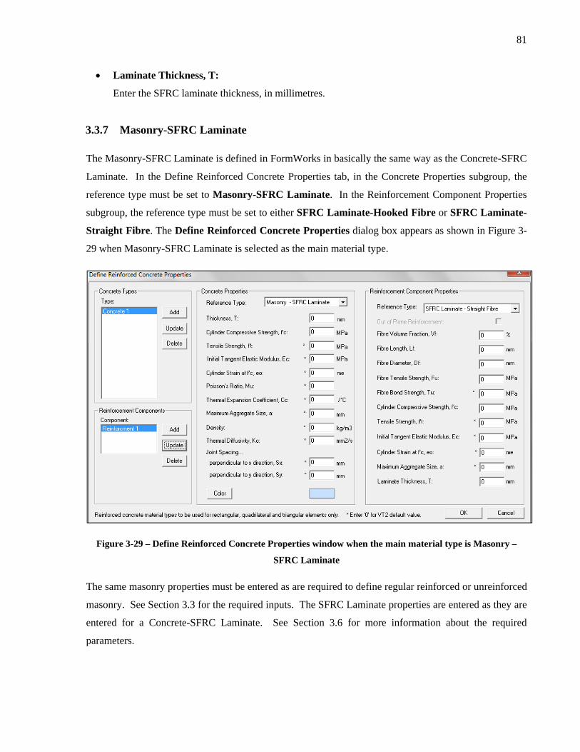
81

Laminate Thickness, T:

Enter the SFRC laminate thickness, in millimetres.

3.3.7 Masonry-SFRC Laminate

The Masonry-SFRC Laminate is defined in FormWorks in basically the same way as the Concrete-SFRC

Laminate. In the Define Reinforced Concrete Properties tab, in the Concrete Properties subgroup, the

reference type must be set to Masonry-SFRC Laminate. In the Reinforcement Component Properties

subgroup, the reference type must be set to either SFRC Laminate-Hooked Fibre or SFRC Laminate-

Straight Fibre. The Define Reinforced Concrete Properties dialog box appears as shown in Figure 3-

29 when Masonry-SFRC Laminate is selected as the main material type.

Figure 3-29 – Define Reinforced Concrete Properties window when the main material type is Masonry –

SFRC Laminate

The same masonry properties must be entered as are required to define regular reinforced or unreinforced

masonry. See Section 3.3 for the required inputs. The SFRC Laminate properties are entered as they are

entered for a Concrete-SFRC Laminate. See Section 3.6 for more information about the required

parameters.

82

3.3.8 Concrete-Ortho Laminate

The Concrete-Ortho Laminate is a combination of a concrete core and wood (or other orthotropic

material) faceplates. Concrete-wood laminates are commonly used in both floor and beam construction.

In new floor construction, solid concrete is typically placed on timber floor beams or a solid layer of

wood. The wood layer functions to replace the cracked concrete-steel reinforcement section of a solid

concrete slab, and also reduces the need for formwork. Similarly, deep beams benefit from concrete-

wood composite construction, as wood can help reduce or eliminate the high tensile stresses in the

concrete. Hence, bridges can also utilize composite concrete-timber decks. As with other laminates,

forces must be transferred between the concrete and the wood, most likely through shear studs. For the

stress-strain behaviour of orthotropic wood, see Figure 3-22 (Gutkowski, et al., 2010).

In the Define Reinforced Concrete Properties tab, in the Concrete Properties subgroup, the reference type

must be set to Concrete-Ortho Laminate. In the Reinforcement Component Properties subgroup, the

reference type must be set to Orthotropic Laminate. The Define Reinforced Concrete Properties

dialog box appears as shown in Figure 3-30 when Concrete-Ortho Laminate is selected as the main

material type.

Figure 3-30 – Define Reinforced Concrete Properties window when the main material type is Concrete–

Ortho Laminate

83

The same concrete properties must be entered as are required to define regular reinforced concrete. See

Section 3.1 for the required concrete inputs.

In Reinforcement Component Properties group, the inputs required are the same as for the Wood (Fixed

Orthotropic) material type, with the exception of density. The wood density is not a required input for

Orthotropic Laminate. The required inputs are specified in Section 3.3.4.

84

Chapter 4

Modeling 3D Solid Structures

4.1 Introduction

VecTor3 is a nonlinear finite element analysis (NLFEA) program for modeling 3D reinforced concrete

solid structures. The theoretical bases of VecTor3 are the Modified Compression Field Theory (Vecchio

and Collins, 1986) and the Disturbed Stress Field Model (Vecchio, 2000). The program uses a smeared,

rotating-crack formulation to analyze the structures. To produce a stable and robust nonlinear solution,

VecTor3 uses a total-load iterative procedure with a secant stiffness formulation.

Incorporated into the program’s analysis algorithms are material nonlinearity effects including

compression softening due to transverse cracking, tension stiffening, shear slip along crack surfaces, and

other mechanisms important in making a precise assessment of cracked reinforced concrete behaviour. In

addition, the program is capable of modeling nonlinear expansion and confinement, cyclic loading,

effects of slip distortion on element compatibility relations, and application to the analysis of repaired or

rehabilitated structures. To consider each of the above mentioned constitutive responses and mechanisms

properly, the program supports a wide range of material models (Selby, 1990).

To create finite element models, VecTor3 utilizes a fine mesh of low-powered elements. The program’s

element library includes an 8-node brick element (24 d.o.f.), a 6-node wedge element (18 d.o.f.), and a 2-

node truss bar element (6 d.o.f.). The solid elements can be used to model reinforced concrete structures.

Reinforcement can be modeled either as smeared within the solid elements, or as discrete bars using the

truss elements. Calculating the stiffness matrix coefficients explicitly for each of the elements makes the

computational time shorter and avoids numerical instabilities such as zero energy nodes or shear locking

in the program analysis (Selby, 1990).

VecTor3 is currently configured to accommodate: 12000 elements, 15000 nodes, 45 concrete material

types, 15 steel material types, and 4 smeared reinforcement components per material type.

Previous versions of FormWorks were only compatible with VecTor2. The remaining VecTor programs

did not have pre-processors and they ran in a DOS environment from Fortran executable files; standard

text editors were used to create input data files. A new version of FormWorks, FormWorks-Plus, has

been developed to create finite element models compatible with the remaining VecTor programs

including VecTor3. FormWorks-Plus is able to create 3D solid finite element models, apply different

85

types of loads, assign material properties, and specify analysis parameters which are compatible with

VecTor3. This chapter will discuss the different parts of FormWorks-Plus that are involved in modeling

a 3D solid structure to be analyzed by VecTor3.

4.2 The Job Data

For the most part, the input properties required to define the Job Page for the 3D Solid Structures are

similar to the input requirements for the 2D Plane Membrane Structures. For further instruction on how

to enter these parameters, see Section 2 in Chapter 3. Figure 4-1 and 4-2 show the analysis parameters in

the Job Control Page and Auxiliary Page unique to VecTor3.

Figure 4-1 – The Job Control Page for 3D Solid Structures

86

Figure 4-2 – The Auxiliary Page for 3D Solid Structures

The input parameters unique to the 3D Solid Structures are:

Initial Load Stage

In the Job Control Page, Enter the load stage number from which the load case should be

activated. The default value is 0.

Time Integration Method

In the Auxiliary Page, Select one of the following Time Integration methods for Dynamic

Analysis. As shown in the following, each method has its own Newmark Beta Factor (β and

Gamma Factor (γ . The default option is the Newmark Constant method.

87

1. Newmark Constant: β 0.25 and γ 0.5.

2. Newmark Linear: β 1/6 and γ 0.5.

3. Newmark Beta: β 0.25 and γ 0.5.

Ground Acceleration in z-direction

In the Dynamic Analysis part of the Auxiliary Page, Choose ‘Considered’ or ‘Not Considered’

for the ground acceleration in the z-direction. The Considered option is to be chosen when the

Analysis Mode on the Job Control page is set to Dynamic Nonlinear—General.

Note that although all the input parameters in the Models Page are similar to the 2D Plane Membrane

Structures, each drop list contains models which are only applicable to the 3D Solid Structures.

4.3 The Structure Data

After defining the analysis parameters and behavioural models in the Job Data Page, the next step is to

define the Structure Data which creates the structure file with a *.S3R extension. This file contains all

the information about the finite element mesh including material properties, node numbers and

coordinates, elements, and restraints.

The first step is to simplify the actual structure so it can be modeled easily with FormWorks-Plus using

cubic and wedge elements. In defining complex finite element models, drawing a sketch can help to have

a better understanding of the model. The sketch should include the simplified geometry of structure,

different reinforced concrete material types, the location of reinforcements and boundary conditions.

Currently FormWorks-Plus is not capable of meshing 3D Solid Structures automatically; only the

manual method is available. Although defining the nodes and elements manually is time consuming, it

gives complete control over the mesh topology and its computational characteristics to the user. To

define the finite element mesh the following steps should be taken:

1. Define material properties

2. Specify nodal coordinates

3. Define elements

4. Assign materials to elements

5. Define restraints

There are several parameters that can affect the finite element mesh such as element types, location of

loads, placement of restraints, number of material types, the required degree of accuracy and processing

88

limits (Wong, 2002). One of the important parameters in meshing the structure is the size of elements.

VecTor3 uses the formulation of the Modified Compression Field Theory to analyze structures. Elements

should be sized so that the distributions of the stress and crack stay uniform within elements. Checking

the analysis results and stress variations in elements may indicate the need for refining the mesh.

4.3.1 Specifying Material Properties

VecTor3 includes two types of materials: reinforced concrete and reinforcement.

4.3.1.1 Reinforced Concrete

For the most part, the input properties required to define the reinforced concrete material in VecTor3 are

similar to the input requirements for VecTor2. For further instruction on how to enter these parameters,

see the FormWorks manual. The input parameters unique to VecTor3 are:

Average Crack Spacing perpendicular to z-reinforcement:

Enter the crack control parameter indicating the spacing of cracks planes perpendicular to the z-

axis for Sz, in millimeters. The default value is computed by the CEB-FIP model, unless the

Tension Chord (Kauffmann) model is selected for tension stiffening.

Reinforcement Orientation:

In VecTor3, instead of defining the “Out-of-Plane Reinforcement” and “Reinforcement Direction

from X-Axis”, direction cosines are used to define the orientation of smeared reinforcement.

Figure 4-3 – Cosine directions for defining reinforcement orientation

89

k, l, and m are direction cosines, defined as the following:

Figure 4-3 demonstrates the definition of the cosine directions. For instance, to define a smeared

reinforcement in the X-direction the input parameters are k = 1, l = 0, and m = 0.

Figure 4-4 – Define Reinforced Concrete Properties window for 3D Solid Structures

4.3.1.2 Reinforcement

The input properties required to define discrete reinforcement in VecTor3 are similar to the input

requirements for VecTor2. For further instruction on how to enter these parameters, see the FormWorks

manual.

90

4.3.2 Defining Nodes

Select the Structure/Create Nodes menu item or click the Create Nodes toolbar button. The Create

Nodes dialog box appears as shown in Figure 4-5. This section explains the procedures to add or delete

nodes. There are two rules for defining the nodes in VecTor programs. The first is that all the nodes of a

finite element mesh must be numbered consecutively starting from 1. The second rule is that all the

nodes must be attached to at least one element.

FormWorks-Plus checks both rules to make sure all nodes are defined correctly. For the first rule the

program allows nodes to be arbitrarily numbered, but when generating the structure file it checks the

node numbers and if the rule is violated FormWorks-Plus renumbers the nodes automatically. For the

second rule, if there is any node which is not attached to an element FormWorks-Plus sends a warning

message to the user.

Renumbering the nodes is a useful feature which allows modifying an existing mesh instead of defining a

new one. But it is recommended that the user follows the above mentioned rules in defining the nodes,

and not rely on the renumbering feature whenever possible.

Figure 4-5 – Create Nodes window for 3D Solid Structures

The coordinates of each node must be defined in the Create Nodes window. Since creating nodes one by

one takes considerable time, FormWorks-Plus has a node increment feature which helps to define several

nodes in the X, Y, and Z directions simultaneously. The following example shows how to use node

increment feature.

Figure 4-6 (A) – A simple example of node increment feature - input data

91

Figure 4-6 (B) – A simple example of node increment feature – 3D view

Figure 4-6(C) – A simple example of node increment feature – Sectional view

By adding or deleting the nodes, the total number of nodes and the drop list in the drop box, showing the

list of the nodes, will be updated automatically. Note that by deleting the nodes, all the nodal loads

assigned to them are also deleted.

4.3.3 Defining Elements

As explained before, VecTor3 has three types of elements: hexahedral elements, wedge elements, and

truss bars. This section explains how to use the VecTor3 elements to create the finite element model in

the FormWorks-Plus. Note that all the elements of a finite element mesh must be numbered

consecutively starting from 1. FormWorks-Plus allows elements to be arbitrarily numbered but, when

generating the structure file, it checks the element numbers and if the rule is violated FormWorks-Plus

Increment by 200 mm in Z direction

Increment by 100 mm in X direction

Increment by 50 mm in Y direction

X=50 Node 1 Y=75 Z=100

92

renumbers the elements automatically. Renumbering the elements is a useful feature which allows

modifying an existing mesh instead of defining a new one.

Hexahedral Elements

The hexahedral element (or brick element) is an 8-node element with 24 degrees of freedom. Select the

Structure/Create Hexahedral Elements menu item or click the Create Hexahedral Elements toolbar

button. The Create Hexahedral Elements dialog box appears as shown in Figure 4-8 (C).

To generate an element, enter all 8 nodes and click the add button. The drop list in the drop box shows

the list of all defined elements. To delete an element, select it from the drop list and click the delete

button. The total number of elements and the drop list contents will be updated automatically by adding

or deleting any element. The default colour for hexahedral elements is white.

FormWorks-Plus has two rules in defining hexahedral elements:

1. The first four nodes must have equal z coordinates and the value must be greater than the last four

nodes z coordinates. This implies that, the first four nodes must be located at the front face and the

last four nodes must be in the back face. (Z1=Z2=Z3=Z4 > Z5=Z6=Z7=Z8)

2. All the element nodes must be defined in a counter-clockwise order in the XY plane.

Figure 4-7 shows a sample hexahedral element defined in FormWorks-Plus:

Figure 4-7 – A sample hexahedral element

Element’s nodes must be entered manually in the dialog box. To save time, FormWorks-Plus has an

element increment feature which allows defining several number of elements simultaneously in two

directions. The following example shows how to use the increment feature for brick elements.

Y

X

Z

93

Figure 4-8 (A) – A simple example of creating brick elements using increment feature – 3D view

Figure 4-8 (B) – A simple example of creating brick elements using increment feature – Sectional view

Z

X Y

Increment in X direction

Increment in Y direction

Element 1

94

Figure 4-8 (C) – A simple example of creating brick elements using increment feature – Input data

Wedge Elements

The wedge element is a 6- node element with 18 degrees of freedom which assumes linear displacement

fields similar to brick elements. Select the Structure/Create Wedge Elements menu item or click the

Create Wedge Elements toolbar button. The Create Wedge Elements dialog box appears as shown in

Figure 4-10 (A).

To generate a wedge element, enter all 6 nodes and click the add button. The drop list in the drop box

shows the list of all the defined elements. To delete an element, select it from the drop list and click the

delete button. The total number of elements and the drop list contents will be updated automatically by

adding or deleting any element. The default colour for wedge element is white.

FormWorks-Plus allows defining three types of wedge elements. Table 4-1 describes the different types

of wedge elements available and the rules to generate these elements. Note that, same as with hexahedral

elements, in wedge elements all the nodes must be defined in a counter-clockwise order.

Wedge Element Types

Type Rules

1

1. In XY plane, The first three nodes must be located at front face and last three nodes must be in back face.

(Z1=Z2=Z3) > (Z4=Z5=Z6)

2. The first node in each face must have the maximum Y coordinate. (Y1>Y2&Y3) , (Y4>Y5&Y6)

2

1. In XZ plane, The first three nodes must be located at front face and last three nodes must be in back face.

(Y1=Y2=Y3) > (Y4=Y5=Y6)

2. The first node in each face must have the maximum Z coordinate. (Z1>Z2&Z3) , (Z4>Z5&Z6)

3

1. In ZY plane, The first three nodes must be located at front face and last three nodes must be in back face.

(X1=X2=X3) > (X4=X5=X6)

2. The first node in each face must have the maximum Z coordinate. (Z1>Z2&Z3) , (Z4>Z5&Z6)

Table 4-1 –Different types of wedge element

95

As explained in Table 4-1, the triangular faces of elements must be parallel to one of the main planes.

The current version of FormWorks-Plus is not capable of modeling an arbitrary shape of wedge element.

Figure 4-9 illustrates the three types of wedge elements available in FormWorks-Plus.

An element’s nodes must be entered manually in the dialog box. To save time, FormWorks-Plus has an

element increment feature which allows defining several number of elements simultaneously in two

directions. The following example shows how to use increment feature for wedge elements.

Figure 4-9 –Different types of wedge element

Figure 4-10 (A) – Create Wedge Elements window

96

Figure 4-10 (B) – The Increment feature for wedge elements – Different views

Truss Elements

The third type of element in VecTor3 is the Truss Bar. Truss elements are mainly used to model

reinforcement discretely. Select the Structure/Create Truss Elements menu item or click the Create

Truss Elements toolbar button to define truss bars.

To generate a truss element enter two node numbers that define the end nodes of element and click the

add button. The drop list in the drop box shows the list of all the defined elements. To delete an element,

select it from the drop list and click the delete button. The total number of elements and the drop list

contents will be updated automatically by adding or deleting any element. The default colour for truss

elements is magenta.

Increment elements in Z direction

97

As with hexahedral and wedge elements, the element increment feature can be used to define multiple

truss bars in two directions simultaneously.

4.3.4 Assigning Materials

The input properties required to assign material types in VecTor3 are similar to the input requirements

for VecTor2. For further instruction on how to enter these parameters, see the FormWorks manual.

4.3.5 Support Restraints

Without restraining the structure, the finite element model is not complete and FormWorks-Plus will not

allow generating the structure file. To add or delete restraints, select the Structure/Create Support

Restraints menu item or click the Create Support Restraints toolbar button. The Create Support

Restraints dialog box appears, as shown in Figure 4-11.

Figure 4-11 – Create Support Restraints window

For the most part, the input properties required to define the support restraints in VecTor3 are similar to

the input requirements for VecTor2. For further instruction on how to select the nodes and enter these

parameters, refer to the FormWorks manual. The only unique input parameter for 3D Solid Structures is

DZ which restraints the selected nodes against displacement in the Z-direction.

4.4 The Load Case Data

The last step in defining the finite element model is assigning the loads. VecTor3 supports six types of

nodal loads, three types of element loads, and ground acceleration load. This section will discuss all

different types of loads and required input parameters.

98

4.4.1 Nodal Loads

4.4.1.1 Joint Loads

Select the Load/Apply Nodal Loads menu item or click the Nodal Loads toolbar button. The Apply

Nodal Loads dialog box appears as shown in Figure 4-12.

Figure 4-12 – Apply Nodal Loads window

The procedure for adding Joint Loads in VecTor3 is similar to that in VecTor2. For further instruction on

how to select the nodes and enter the parameters, refer to the FormWorks manual. The unique entry

fields are described as follows:

Fz:

Enter the joint force acting in Z-direction, in kN. Positive values represent the force in the

direction of positive X-axis, while negative values are in the opposite direction.

dFz:

Enter the increment of the force in Z-direction for the selected nodes, in kN.

4.4.1.2 Support Displacements

Select the Load/Apply Support Displacement menu item or click the Support Displacement toolbar

button. The Apply Support Displacement dialog box appears as shown in Figure 4-13.

Figure 4-13 – Apply Support Displacements window

99

The procedure for adding Joint Loads in VecTor3 is similar to that in VecTor2. For further instruction on

how to select the nodes and enter the parameters, refer to the FormWorks manual. The only unique entry

field is degree of freedom (D.O.F) in the Z-direction. Select the X, Y or Z direction to apply nodal

displacement to the selected nodes. To apply displacements in two or three directions, separate entries

are required.

4.4.1.3 Vapour Content

Select the Load/Apply Nodal Vapour Content menu item or click the Nodal Vapour Content toolbar

button. The Apply Nodal Vapour Content dialog box appears as shown in Figure 4-14.

Figure 4-14 – Apply External Nodal Vapour window

Enter the node number or use the select button to specify the nodes with external vapour content. To

delete a vapour content select the entry either from the drop list or using the select feature and click the

delete button.

4.4.1.4 Nodal Thermal Loads

Select the Load/Apply Nodal Thermal Loads menu item or click the Nodal Thermal Loads toolbar

button. The Apply Nodal Thermal Loads dialog box appears as shown in Figure 4-15.

Figure 4-15 – Apply Nodal Thermal Loads window

100

Enter the node number or use the select feature to specify the nodes with thermal loads. To define a

thermal load, complete the following input parameters.

Table 4-2 – Different types of Standard Fire Curves (Zhou, 2004)

101

Surface:

Specify the surface for which the temperature parameters are going to be defined.

1. Atmosphere

2. Element Surface

The default option is to apply the temperature parameters of the atmosphere.

Fire Curve Type:

Enter one of the following Standard Fire Curves:

1. Steady- State

2. Three-Key-Node Linear Model

3. Compartment Simplified Fire Model

4. ASTM-E119 Fire Model

5. ISO-834 Fire Model

The default model is number 1, Steady-State. For more information about the different types of

Standard Fire Curves see Table 4-2.

Tm (n):

Enter the time, in seconds, at which the temperature Tp (n) occurs.

Tp (n):

Enter the temperature, in °C, corresponding to Tm (n).

Tcool:

Enter the time, in seconds, at which the cooling process starts.

To delete a thermal load select the entry either from the drop list or using the select feature and click the

delete button.

4.4.1.5 Lumped Masses

Select the Load/Apply Lumped Masses menu item or click the Lumped Masses toolbar button. The

Apply Lumped Masses dialog box appears as shown in Figure 4-16. Note that this load type is only

applicable when performing dynamic analysis.

102

Figure 4-16 – Apply Lumped Masses window

Enter the node number or use the select feature to specify the nodes with lumped mass. To define a

lumped mass load complete the following input parameters:

DOF:

Select the Degree Of Freedom (DOF) in which Lumped Mass is applied. It is possible to select

more than one direction.

Mass:

Enter the lumped mass, in kg, acting on the selected nodes.

GF-X, Y or Z:

Enter the factor of ground acceleration acting in X, Y, and Z direction, expressed in g (9.81 m/

s .

Note: In VecTor4, the ground acceleration values are in m/s , not in terms of g. For instance to

apply 4g ground acceleration in the X-direction, the input parameter in VecTor3 must be 4, while

in VecTor4 it must be 4 9.81 39.24 / .

Vo-X, Y or Z:

Enter the initial velocities, in m/s, acting on the selected nodes in X, Y, and Z direction.

4.4.1.6 Impulse Forces

Select the Load/Apply Impulse Forces menu item or click the Impulse Forces toolbar button. The

Apply Impulse Forces dialog box appears as shown in Figure 4-17.

Figure 4-17– Apply Impulse Forces window

103

The procedure for adding the impulse forces in VecTor3 is similar to that in VecTor2. For further

instruction on how to select the nodes and enter the parameters, refer to the FormWorks manual. The

only unique entry field is the Degree Of Freedom (D.O.F.) in the Z-direction. Select one of the X, Y, or

Z directions to apply impulse forces to the selected nodes. To apply impulse forces in two or three

directions at the same node, separate entries are required.

4.4.2 Element Loads

4.4.2.1 Gravity Loads

Select the Load/Apply Gravity Loads menu item or click the Gravity Loads toolbar button. The Apply

Gravity Loads dialog box appears as shown in Figure 4-18.

Figure 4-18 – Apply Gravity Loads window

The procedure for adding the gravity loads in VecTor3 is similar to that in VecTor2. For further

instruction on how to select the nodes and enter the parameters, refer to the FormWorks manual. The

only unique entry field is the G-force acting in the Z-direction, GZ. For gravity forces acting in the

positive direction of Z-axis enter positive values. The GZ parameter can be used when the coordinate

axes have been rotated and a component of the gravitational load is acting in the Z-direction.

4.4.2.2 Temperature Loads

The input properties required to apply temperature loads in VecTor3 are similar to the input requirements

for VecTor2 program. For further instruction on how to enter these parameters, refer to the FormWorks

manual.

4.4.2.3 Concrete Prestrains

The input properties required to apply concrete prestrains in VecTor3 are similar to the input

requirements for VecTor2 program. For further instruction on how to enter these parameters, refer to the

FormWorks manual.

104

4.4.3 Ground Accelerations

Select the Load/Apply Ground Acceleration menu item or click the Ground Acceleration toolbar

button. The Apply Ground Acceleration dialog box appears as shown in Figure 4-19.

Figure 4-19 – Apply Ground Acceleration window

The procedure for adding the ground acceleration in VecTor3 is similar to that in VecTor2. For further

instruction on how to select the nodes and enter the parameters, see the FormWorks manual. The only

unique entry field is Acc Z (G). Acc Z (G) is the ground acceleration in the Z direction, in m/s2,

occurring at the specified time.

4.5 A Simple Example in VecTor3 In this section, a simple example illustrating the FormWorks-Plus modeling procedure for 3D solid

structures is presented. The objective of the example is to create a finite element model for a reinforced

concrete beam with hollow section, and investigate the response of the structure under combined flexure

and torsion. The beam to be modeled is one tested by Onsongo in 1978. Figure 4-20 and 4-21

demonstrate the testing arrangement and the cross sectional properties, respectively.

Figure 4-20 – Test arrangement for bending-torsion beam (Osongo, 1978).

105

Figure 4-21 – The cross sectional properties

To save time in performing the analysis, only a part of the test beam considered in the finite element

model. Since the beam is subjected to constant moment and torque along its length this simplification

does not affect the results. Figure 4-22 shows the detailed meshing of the structure created by

FormWorks-Plus. For modeling the transverse reinforcements properly, three elements were used

through the thickness of the webs and flanges. To maintain the size of elements reasonable in all

directions, 10 layers of elements were used along the length of the structure.

Figure 4-22 – The mesh used for the finite element model

106

Both the longitudinal and hoop reinforcement were modeled as smeared. To make the theoretical model

more realistic, two-thirds of the hoop reinforcement was smeared in the outermost layer of elements. The

remaining area of the reinforcement was smeared over the inner two layers of elements (Vecchio, et al.,

1990). Table 4-3 and Figure 4-23(a) show the material type’s properties and the location of each material

type in the structural model, respectively.

Following figure demonstrates the finite element mesh, generated by FormWorks-Plus.

Figure 4-23 – The finite element mesh generated by FormWorks-Plus and the location of each material type

107

Material Type

Concrete Properties Reinforcement Component Properties

Colour F'c F't Ec e0 Other

Properties Comp.

#

Orientation ρ Db Fy Fu Es esh eu

MPa MPa MPa me k l m % mm MPa MPa MPa me me

1

34.8 1.95 32445 3.1 default 1 1 0 0 1.229 12.7 393 600 200000 10 100

2 0 0 1 1.016 12.7 393 600 200000 10 100

2

34.8 1.95 32445 3.1 default 1 0 1 0 1.229 12.7 393 600 200000 10 100

2 0 0 1 0.793 9.525 401 600 200000 10 100

3

34.8 1.95 32445 3.1 default 1 1 0 0 1.229 12.7 393 600 200000 10 100

2 0 0 1 9.352 25.4 436 600 200000 10 100

4

34.8 1.95 32445 3.1 default 1 0 1 0 4.914 12.7 393 600 200000 10 100

2 0 0 1 1.016 12.7 393 600 200000 10 100

5

34.8 1.95 32445 3.1 default 1 0 1 0 4.914 12.7 393 600 200000 10 100

2 0 0 1 9.352 25.4 436 600 200000 10 100

6

34.8 1.95 32445 3.1 default 1 1 0 0 4.914 12.7 393 600 200000 10 100

2 0 0 1 1.016 12.7 393 600 200000 10 100

7

34.8 1.95 32445 3.1 default 1 0 1 0 4.914 12.7 393 600 200000 10 100

2 0 0 1 0.793 9.525 401 600 200000 10 100

8

34.8 1.95 32445 3.1 default 1 1 0 0 4.914 12.7 393 600 200000 10 100

2 0 0 1 9.352 25.4 436 600 200000 10 100

9

34.8 1.95 32445 3.1 default

1 1 0 0 4.914 12.7 393 600 200000 10 100

2 0 1 0 4.914 12.7 393 600 200000 10 100

3 0 0 1 1.016 12.7 393 600 200000 10 100

10

34.8 1.95 32445 3.1 default

1 1 0 0 4.914 12.7 393 600 200000 10 100

2 0 1 0 4.914 12.7 393 600 200000 10 100

3 0 0 1 9.352 25.4 436 600 200000 10 100

11

34.8 1.95 32445 3.1 default

1 1 0 0 1.229 12.7 393 600 200000 10 100

2 0 1 0 1.229 12.7 393 600 200000 10 100

3 0 0 1 1.016 12.7 393 600 200000 10 100

12

34.8 1.95 32445 3.1 default

1 1 0 0 1.229 12.7 393 600 200000 10 100

2 0 1 0 1.229 12.7 393 600 200000 10 100

3 0 0 1 9.352 25.4 436 600 200000 10 100

Table 4-3 – Material properties

108

The bending moments and torques were applied as nodal forces at the end of the beam. The ratio of the

torsion to moment was 1.47. To avoid end failure and facilitate load transfer, a stiffer material was

assigned to the elements in the final layer. Two load cases were defined in FormWorks-Plus, the Torsion

load case and the Moment load case. The load factor was increased monotonically from zero to failure in

increments of 1. Following is the VecTor3 analysis results:

& (Note: T/M factor equals to 1.47)

Figure 4-24 –Torsion and moment acting on the structural model

Figure 4-25 –Load-deflection response of the beam

0

1

2

3

4

5

6

7

8

0 1 2 3 4 5

Loa

d f

acto

r

dx (mm)

Load-Displacement Response

109

Figure 4-26 –Deformed shape of structure under combined torsion and moment loads

110

Chapter 5

Modeling Shell Structures

5.1 Introduction

VecTor4 is a nonlinear finite element analysis (NLFEA) program for reinforced concrete shell and plate

structures. The theoretical basis for VecTor4 is the Disturbed Stress Field Model (Vecchio, 2000) which

is derived from the Modified Compression Field Theory (Vecchio and Collins, 1986). The program uses

a smeared rotating-crack formulation to analyze concrete structures. VecTor4 assumes a constant normal

shear strain through the thickness of the elements to account for transverse shear deformations.

To generate a finite element model, VecTor4 utilizes degenerated quadratic isoparametric shell elements;

specifically, a 9-node heterosis element with 42 degrees of freedom. Using quadratic shape functions

allows the program to model curved surfaces. All side and corner nodes have three translational and two

rotational degrees of freedom; the central ninth node has only the two rotational degrees of freedom. A

principal advantage of the Heterosis element is that it exhibits good behaviour for both thick and thin

shells (Seracino, 1995). Since it is one of the Mindlin type elements, its formulation is based on the

following assumptions:

1. ‘Normals’ to the mid-surface remain straight but not necessarily normal after deformation, and

2. Resultant stresses normal to the mid-surface are negligible.

Figure 5-1 shows a typical 9-node heterosis element used in the program formulation.

Figure 5-1 – A 9-node heterosis element

Incorporated into the program’s analysis algorithms are material nonlinearity effects such as compression

softening due to transverse cracking, tension stiffening, shear slip along crack surfaces, and other

mechanisms important in accurately representing the behaviour of cracked reinforced concrete structures.

To model material properties, VecTor4 employs a layered element formulation. Each material type can

have up to 50 layers of concrete, where each layer has the same thickness and concrete properties. Steel

111

layers are superimposed to model the in-plane reinforcement. Out-of-plane (transverse shear)

reinforcement is defined as a property of the concrete layers.

The program is currently configured to accommodate: 600 elements, 3000 nodes. 35 concrete/steel

material types, 50 concrete layers per material type, and 10 smeared reinforcement components per

material type.

VecTor4 does not have pre-processor; it runs in a DOS environment from Fortran executable files.

Creating finite element models without any graphical tool, especially with the complex heterosis

element, is time consuming and can cause meshing problems. A user-friendly pre-processor,

FormWorks-Plus, has been developed to create finite element models compatible with the analysis

program. FormWorks-Plus is able to create shell element models, apply different types of loads, assign

material properties, and specify analysis parameters that are compatible with VecTor4. This chapter will

discuss the different parts of FormWorks-Plus that are involved in modeling a shell structure to be

analyzed by VecTor4.

5.2 The Job Data

For the most part, the input properties required to define the Job Page for the Shell Structures are similar

to the input requirements for the 3D Solid Structures. For further instruction on how to enter these

parameters, see Section 2 in Chapter 4. The Auxiliary page is the only part that has input parameters

unique to Shell Structures:

Shear Analysis Mode

Select one of the following models for the shear analysis mode:

1. Uniform Shear Strain

2. Parabolic Shear Strain

3. No Out-of-Plane Shear

The default model is option 2, Parabolic Shear Strain.

Mass Factor due to Self-Weight

In dynamic analysis, to consider the nodal lumped masses due to the self-weight of the structure,

a nonzero factor must be applied. Note that self-masses are only used in dynamic analyses; they

are not converted to static forces. The default value is 1.0 which corresponds to the unfactored

self-mass of the structure.

112

Figure 5-1 shows unique analysis parameters for VecTor4 in the Auxiliary Page.

Figure 5-2 – The Auxiliary Page for Shell Structures

Note that although all the input parameters in the Models Page are similar to the inputs for the previous

types of structures discussed in Chapter 3 and 4, each drop list contains models which are only applicable

to Shell Structures.


After defining all analysis parameters and behavioural models in the Job Data Page, the next step is to

define the Structure Data which creates a structure file with the *.S4R extension. This file contains

information about the finite element mesh including material properties, node numbers and coordinates,

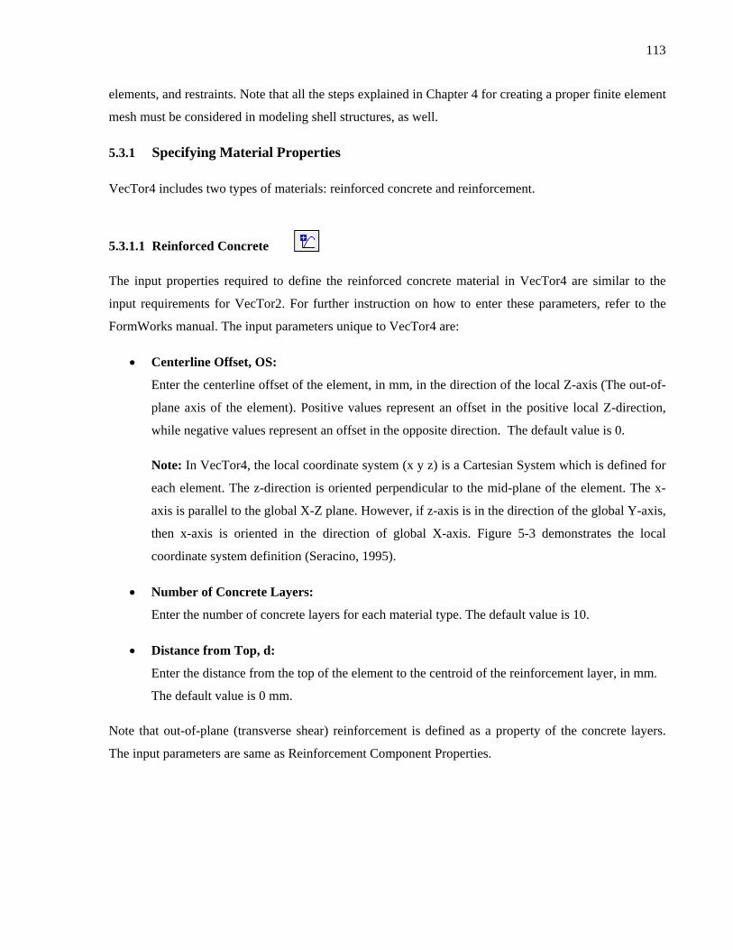
113

elements, and restraints. Note that all the steps explained in Chapter 4 for creating a proper finite element

mesh must be considered in modeling shell structures, as well.


VecTor4 includes two types of materials: reinforced concrete and reinforcement.

5.3.1.1 Reinforced Concrete

The input properties required to define the reinforced concrete material in VecTor4 are similar to the

input requirements for VecTor2. For further instruction on how to enter these parameters, refer to the

FormWorks manual. The input parameters unique to VecTor4 are:

Centerline Offset, OS:

Enter the centerline offset of the element, in mm, in the direction of the local Z-axis (The out-of-

plane axis of the element). Positive values represent an offset in the positive local Z-direction,

while negative values represent an offset in the opposite direction. The default value is 0.

Note: In VecTor4, the local coordinate system (x y z) is a Cartesian System which is defined for

each element. The z-direction is oriented perpendicular to the mid-plane of the element. The x-

axis is parallel to the global X-Z plane. However, if z-axis is in the direction of the global Y-axis,

then x-axis is oriented in the direction of global X-axis. Figure 5-3 demonstrates the local

coordinate system definition (Seracino, 1995).

Number of Concrete Layers:

Enter the number of concrete layers for each material type. The default value is 10.

Distance from Top, d:

Enter the distance from the top of the element to the centroid of the reinforcement layer, in mm.

The default value is 0 mm.

Note that out-of-plane (transverse shear) reinforcement is defined as a property of the concrete layers.

The input parameters are same as Reinforcement Component Properties.

114

Figure 5-3 – Local coordinates in VecTor4 (Seracino, 1995).

Figure 5-4 – Define Reinforced Concrete Properties window for Shell Structures

115

5.3.1.2 Reinforcement

For the most part, the input properties required to define the reinforcement material in VecTor4 are

similar to the input requirements for VecTor2. For further instruction on how to enter these parameters,

refer to the FormWorks manual. The only unique input parameter to VecTor4 is Centerline Offset (OS)

which has been explained in Section 3.1.1.

Figure 5-5 – Define Reinforcement Properties window for Shell Structures

5.3.2 Defining Nodes

Select the Structure/Create Nodes menu item or click the Create Nodes toolbar button. The Create

Nodes dialog box appears as shown in Figure 5-6. This section explains the procedures for adding or

deleting nodes. Note that the rules for defining the nodes, discussed in Section 3.2 of Chapter 4, must be

considered for Shell Structures as well. FormWorks-Plus checks the rules to make sure all nodes are

defined correctly.

116

Figure 5-6 – Create Nodes window for Shell Structures

As discussed in the first chapter, FormWorks-Plus has two options for specifying node coordinates: Top

(In) and Bottom (Out) or Centerline node coordinates. The default option is Top/Bottom coordinate type.

To display the bottom coordinates of the nodes on the screen, check the Node Numbers (Out/Bot.) box in

the Display Options window. By selecting Centerline coordinate type from the drop list, the input

parameters for coordinates will reduce from 6 to 3 automatically. The Top (In) and Bottom (Out)

coordinates option is mainly used for modeling curved structures; Centerline coordinates are suitable for

modeling slabs and beams.

For Shell Structures, the coordinates of each node must be defined manually in the Create Nodes

window. Since creating nodes one by one is a time consuming process, as with other structural types,

FormWorks-Plus allows the user to define the nodes by a node increment feature.

By adding or deleting the nodes, the total number of nodes and the drop list in the drop box, showing the

list of the nodes, will be updated automatically. Note that by deleting nodes, all the nodal loads assigned

to them are also deleted.

5.3.3 Defining Elements

VecTor4 has two types of elements: heterosis shell elements and truss bars. This section explains how to

use these elements to create a finite element model in FormWorks-Plus. Note that all the elements of a

finite element mesh must be numbered consecutively starting from 1. As with other structural types,

FormWorks-Plus allows heterosis elements to be arbitrarily numbered. However, when generating the

structure file, FormWorks-Plus checks the element numbers and if the rule is violated, it renumbers the

elements automatically.

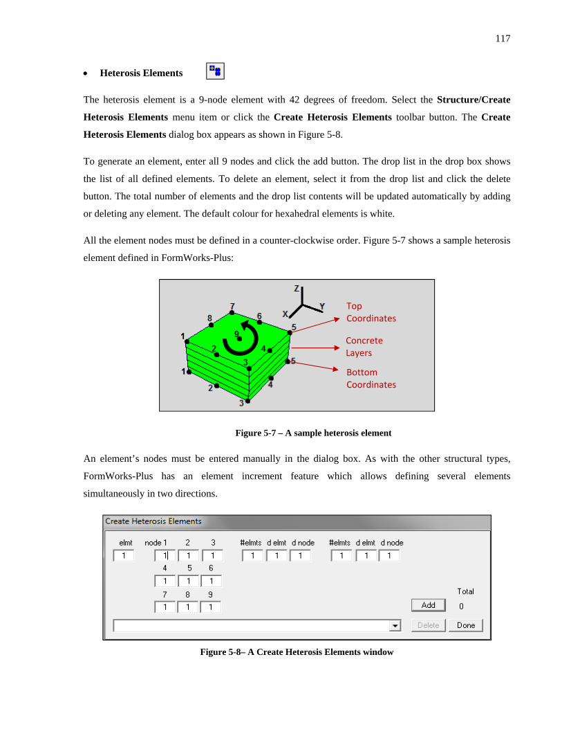
117

Heterosis Elements

The heterosis element is a 9-node element with 42 degrees of freedom. Select the Structure/Create

Heterosis Elements menu item or click the Create Heterosis Elements toolbar button. The Create

Heterosis Elements dialog box appears as shown in Figure 5-8.

To generate an element, enter all 9 nodes and click the add button. The drop list in the drop box shows

the list of all defined elements. To delete an element, select it from the drop list and click the delete

button. The total number of elements and the drop list contents will be updated automatically by adding

or deleting any element. The default colour for hexahedral elements is white.

All the element nodes must be defined in a counter-clockwise order. Figure 5-7 shows a sample heterosis

element defined in FormWorks-Plus:

Figure 5-7 – A sample heterosis element

An element’s nodes must be entered manually in the dialog box. As with the other structural types,

FormWorks-Plus has an element increment feature which allows defining several elements

simultaneously in two directions.

Figure 5-8– A Create Heterosis Elements window

Top Coordinates

Bottom Coordinates

Concrete Layers

118

Truss Elements

The second type of element in VecTor4 is the Truss Bar. Truss elements are mainly used to model

reinforcement discretely. They can also be used to model external “springs”. Select the

Structure/Create Truss Elements menu item or click the Create Truss Elements toolbar button to

define truss bars.



for VecTor2. For further instruction on how to enter these parameters, refer to the FormWorks manual.


Without restraining the structure, the finite element model is not complete and FormWorks-Plus will not

allow generating the structure file. To add or delete restraints, select the Structure/Create Support

Restraints menu item or click the Create Support Restraints toolbar button. The Create Support

Restraints dialog box appears as shown in Figure 4-11.

Figure 5-9 – Create Support Restraints window

For the most part, the input properties required to define the support restraints in VecTor4 are similar to

the input requirements for VecTor3. The unique input parameters for Shell Structures are rotational

restraints. Check the R1 and R2 boxes to restraint the selected nodes against rotations about the local

and directions.

Note: In VecTor4, is the nodal coordinate system defined at each nodal point. Its origin

lies on the midsurface of the element, where the subscript k indicates node k. Vector is defined by

the line joining the bottom coordinates of the node k to the top coordinates of node k. Vector is

oriented perpendicular to and parallel to the XZ global plane. However, if is oriented in the

global Y-direction, then is oriented in the global X-direction. Finally, vector is oriented

119

perpendicular to the plane formed by vector and . Figure 5-10 demonstrates the nodal coordinate

system defined in VecTor4.

R1 and R2 are the rotations about the local and directions, respectively. By calculating the

components of rotations, R1 and R2 can be expressed for each element in terms of local coordinate

system, where R1 is the rotation about local y-direction and R2 is the rotation about local x-direction.

Refer to Figure 5-3 for the local coordinate system definition.

Figure 5-10 – Nodal coordinate system in VecTor4 (Seracino, 1995).


The last step in defining the finite element model is assigning the loads. VecTor4 supports four types of

nodal loads, five types of element loads, and ground acceleration load. This section will discuss the

different types of loads and required input parameters. Note that the load types, including Ground

Acceleration, Impulse Forces, Lumped Masses, and Concrete Prestrains, and the input parameters that

are similar to VecTor3 are not described in this section. For instruction on how to define these load types

and input parameters, see Section 4 in Chapter 4.

120

5.4.1 Nodal Loads

5.4.1.1 Concentrated Loads

Select the Load/Apply Concentrated Loads menu item or click the Concentrated Loads toolbar

button. The Apply Concentrated Loads dialog box appears as shown in Figure 5-11.


The unique input parameters to Shell Structures are:

Mxz:

Enter the magnitude of the concentrated bending moment about direction, in kNm. It implies

a bending moment about the local y-direction.

Myz:

Enter the magnitude of the concentrated bending moment about direction, in kNm. It implies

a bending moment about the local x-direction.

5.4.1.2 Prescribed Node Displacements




The unique input parameters to Shell Structures are R1 and R2 which are described in Section 3.5.

121

5.4.2 Element Loads

5.4.2.1 Uniformly Distributed Loads

Select the Load/Apply Uniformly Distributed Loads menu item or click the Uniformly Distributed

Loads toolbar button. The Apply Uniformly Distributed Loads dialog box appears as shown in Figure

5-13. Enter the element number or use the select feature to specify the elements with uniformly

distributed loads. To delete a load, select the entry either from the drop list or using the select feature and

click the delete button.

The pressure input parameter is the magnitude of the uniformly distributed load applied normal to the

elements surface, in MPa, in the direction of local z-axis. A negative value represents a pressure acting

from the top to the bottom surface of the element, while a positive value is a pressure acting in the

opposite direction.

Figure 5-13 – Apply Uniformly Distributed Loads window

5.4.2.2 Hydrostatic Loads

Select the Load/Apply Hydrostatic Loads menu item or click the Hydrostatic Loads toolbar button.

The Apply Hydrostatic Loads dialog box appears as shown in Figure 5-14.


Enter the following input parameters for defining the load:

122

Load:

Enter the maximum value of the hydrostatic load, in MPa, in the direction normal to the surface

of the structure.

Z:

Enter the global coordinate of zero hydrostatic pressure, in mm, in the Z-direction.

5.4.2.3 Temperature Loads

Select the Load/Apply Temperature Loads menu item or click the Temperature Loads toolbar button.

The Apply Temperature Loads dialog box appears as shown in Figure 5-15.

The unique input parameters to VecTor4 are:

Final Bottom:

Enter the final temperature change of the bottom surface of the element, in °C.

Initial Bottom:

Enter the initial temperature change of the bottom surface of the element, in °C.

Final Top:

Enter the final temperature change of the top surface of the element, in °C.

Initial Top:

Enter the initial temperature change of the top surface of the element, in °C.

Elapsed:

Enter the elapsed time between the initial and final temperatures, in hours.

Figure 5-15 – Apply Temperature Loads window

5.4.2.4 Gravitational Loads

Select the Load/Apply Gravitational Loads menu item or click the Gravitational Loads toolbar

button. The Apply Gravitational Loads dialog box appears as shown in Figure 5-16. The only unique

123

input parameter to Shell Structures is Gamma, the angular velocity with respect to the global Z-

direction, in m/s.

Figure 5-16 – Apply Gravity Loads window

5.5 A Simple Example in VecTor4

In this section, a simple example illustrating the FormWorks-Plus modeling procedure for Shell

Structures is presented. The purpose is to analyze the failure of a reinforced concrete tank used to supply

agricultural water for farms in India. The problem was referred to the Department of Civil Engineering

of Uttar Pradesh for the remedial measures. Figure 5-17 demonstrates deterioration of concrete due to

environmental effects at the ground level of the tank (Mital, et al., 2008).

Figure 5-17 – A view of the tank at the ground level, showing deterioration of concrete due to environmental

effects (Mital, et al., 2008).

124

Unfortunately, the exact detailed design of the reinforced concrete tank is not available. Figure 5-18 and

5-19 shows the geometry and the cross sectional properties of a water tank which is similar to the one

that failed in India.

Figure 5-18 – Dimensions of the structure

Figure 5-19 – The cross sectional properties

125

The finite element model created by FormWorks-Plus includes 60 nodes and 30 elements for each

circumferential band, with 10 bands of elements used to model the entire height. This results in a total

number of 1260 nodes and 300 shell elements. Figure 5-20 and 5-21 show the element numbering and

node numbering in the finite element model, respectively.

Figure 5-20 – The mesh used for the finite element model-element numbering

Figure 5-21 – The mesh used for the finite element model-node numbering

Eac

h of

the

is 5

00 m

m

5 layers of concrete

126

Figure 5-22 – The finite element model created with FormWorks-Plus

Material Type

Concrete Properties

Colour T # of

Layers

F'c F't Ec e0 Out‐of‐ PlaneReinforcement mm MPa MPa MPa me

1 304.8 5 27.6 1.73 27504 2.007 ‐‐‐

2 304.8 5 27.6 1.73 27504 2.007 ‐‐‐

Table 5-1 (A) – Material properties defined in FormWorks-Plus- Concrete Properties

127

Material Type

Reinforcement Component Properties

Comp. #

Direction As Dist. ‐ Top Db Fy Fu Es esh eu

Degree mm^2/m mm mm MPa MPa MPa me me

1

1 90 947 50.8 19.05 414 500 200000 20 200

2 90 947 254 19.05 414 500 200000 20 200

3 0 315 50.8 19.05 414 500 200000 20 200

4 0 315 254 19.05 414 500 200000 20 200

2

1 90 710 50.8 19.05 414 500 200000 20 200

2 90 710 254 19.05 414 500 200000 20 200

3 0 315 50.8 19.05 414 500 200000 20 200

4 0 315 254 19.05 414 500 200000 20 200

Table 5-1 (B) – Material properties defined in FormWorks-Plus- Reinforcement Components

The structure is analyzed under two load cases, self-weight and water pressure. The gravity load type

with zero increment is used to apply the self-weight of structure. To define water pressure, the pressure

corresponding to each layer of elements is calculated and applied as a uniformly distributed load in

FormWorks-Plus. Figure 5-24 and 5-25 shows the deflected shape and load-deformation response of

structure, respectively.

Figure 5-23 – Deflected shape of structure

128

Figure 5-24 – Load-deflection response of structure

0

10

20

30

40

50

60

70

80

90

0 5 10 15 20 25 30 35 40 45 50 55 60 65

y reaction (KN)

y displacement (mm)

129

Chapter 6

Modeling 2D Frame Structures

6.1 Introduction

VecTor5 is a nonlinear sectional analysis program for reinforced concrete plane frame structures.

Temperature, static and dynamic loading conditions are available in VecTor5. Temperature loads include

nonlinear thermal gradients; static loads include monotonic, cyclic and reversed-cyclic load cases;

dynamic loads include base accelerations (time-history analysis under an input accelerogram), impulse,

impact and blast loads, initial velocity and constant acceleration load cases. Based on the Disturbed

Stress Field Model (Vecchio, 2000) which is derived from the Modified Compression Field Theory

(Vecchio and Collins, 1986), VecTor5 uses a smeared rotating crack approach for reinforced concrete

based on a total load, secant stiffness formulation.

The computational algorithm performs two interrelated analyses. First, VecTor5 performs a global frame

analysis based on direct stiffness method. In the next step, by using a distributed nonlinearity fibre model

approach, rigorous sectional analyses of concrete member cross sections are performed at various

sections along the lengths of the members. The computed responses are enforced with the use of an

unbalanced force approach where the unbalanced forces are reduced to zero iteratively (Guner, 2008).

VecTor5 is capable of considering second order effects including material and geometric nonlinearities,

time- and temperature-related effects, membrane action, nonlinear degradation of concrete and

reinforcement under elevated temperatures, concrete compression softening, tension stiffening and

tension softening, shear slip along crack surfaces, nonlinear concrete expansion, confinement effects,

previous loading history, effects of slip distortions on element compatibility relations, concrete prestrains

and reinforcement dowel action.

The program is currently configured to accommodate: 1200 elements, 1000 nodes. 50 material types, 110

concrete layers per material type, and 30 rebar components per material type.

Creating the structural model in text files without any graphical tool is a complex and time consuming

process. FormWorks-Plus is a user-friendly pre-processor, capable of defining plane frame structures,

applying different types of loads, assigning material properties, and specifying analysis parameters which

are compatible with VecTor5. The program allows the user to define nodes and members based on the

geometry, including joint regions, and specify the properties of concrete layers and rebar components for

130

each material type. This chapter will discuss the different parts of FormWorks-Plus that are involved in

the modeling of a 2D frame structure to be analyzed with VecTor5.

6.2 The Job Data

For the most part, the input properties required to define the Job Page for VecTor5 are similar to the

input requirements for VecTor4. For further instruction on how to enter these parameters, see Section 2

in Chapter 5. The Auxiliary page is the only part that has input parameters unique to Plane Frame

Structures:

Figure 6-1 – The Auxiliary Page for Plane Frame Structures

131

Section Analysis Mode

Select one of the following models for the Section Analysis Mode:

1. Nonlinear Section Analysis

2. Effective Stiffness (Branson’s formula)

3. Cracked/Uncracked (ACI349)

4. Uncracked (Using gross section stiffness)

5. Fully Cracked (Using cracked section stiffness)

The default model is option 1, Nonlinear Section Analysis.

Shear Protection

Experience with VecTor5 has shown that regions where strain distribution is significantly

nonlinear such as near concentrated loads, corners, supports and other discontinuities are

vulnerable to premature shear failures (Guner, 2008). To account for this phenomenon in

discontinuity regions, commonly known as D-regions, an algorithm called shear protection was

introduced into the proposed analysis procedure. Figure 6-2 shows D- and B-regions (where B

refers to beam) for a reinforced concrete frame (Schlaich et al., 1987).

Figure 6-2 – A Reinforced Concrete Frame: (a) B- and D-Regions; (b) Bending Moment Distribution (Schlaich et al., 1987)

In FormWorks-Plus, the shear protection algorithm is considered by default. To turn this feature

off, select “Not Considered” from the drop list.

132

Reference Temperature

The reference temperature is the ambient temperature, in °C, against which the top and bottom

sectional temperatures are defined in a thermal analysis.


Having the extension *.S5R, the Structure Data File contains information regarding nodal coordinates,

member indices, support restraints, member specifications, concrete layers, rebar layers, and detailed

member output list.


VecTor5 and FormWorks-Plus allow the user to define up to 50 material types. Each material type

contains a number of concrete layers and reinforcement components which must be defined from the top

of the section. Some of the input properties required to define the reinforced concrete material are similar

to the input requirements for VecTor2. For further instruction on how to enter these parameters, refer to

the FormWorks manual. The input parameters unique to VecTor5 are shown in Figure 6-3 with

highlighted boxes:

Figure 6-3 – Define Reinforced Concrete Properties window for Plane Frame Structures

133

6.3.1.1 General Properties

Reference type:

Select one of the reference types shown in Figure 6-4 to specify the member behaviour and nodal

degrees-of-freedom.

Figure 6-4 – Member reference types (Guner, 2008)

Transverse Reinforcing Bar Properties:

Enter the properties of the transverse and out-of-plane reinforcement.

6.3.1.2 Concrete Layer Properties

Thickness, Dc:

Enter the thickness of the layer, in mm.

134

Width, Wc:

Enter the width of the cross section, in mm.

Transverse Reinf. Ratio, Rho-t:

Enter the ratio of the transverse reinforcement in the corresponding concrete layer, in %.

Out-of-Plane Reinf. Ratio, Rho-z:

Enter the ratio of the out-of-plane reinforcement in the corresponding concrete layer, in %.

Number of Layers, Nx:

Enter the number of concrete layers with identical details. The default value is 1.

6.3.1.3 Longitudinal Reinforcing Bar Layer Properties

The only unique input parameter is Ys, the location of the longitudinal reinforcement layer measured

from the top of the cross section, in mm.

6.3.2 Defining Nodes and Members

The procedure for defining nodes and members for 2D Frame Structures is similar to defining nodes and

truss bars for Plane Membrane Structures. VecTor5 uses 2-node frame members which are defined based

on orientations described in Figure 6-5, where 1 and 2 show the input order specified by the user for

node numbers; NODE1 and NODE2 are the node numbers that the program uses.

Figure 6-5 – Orientation of frame members (Guner, 2008)

135








The last step in defining the finite element model is assigning the loads. VecTor5 supports four types of

nodal loads, six types of element loads, and ground acceleration load. This section will discuss the

different types of loads and required input parameters. Note that the load types, including Nodal Loads,

Nodal Displacements, Gravity Loads, Temperature Loads, Ground Acceleration, Impulse Forces,

Lumped Masses, and Concrete Prestrains, and the input parameters that are similar to the other types of

structures are not described in this section. For instruction on how to define these load types and input

parameters, see Section 4 in Chapter 4.

6.4.1 Member End Actions

Select the Load/Apply Member End Actions menu item or click the Member End Actions toolbar

button. The Apply Member End Actions dialog box appears as shown in Figure 6-6. Enter the element

number or use the select feature to specify the elements with Member End Actions. To delete a load,

select the entry either from the drop list or using the select feature and click the delete button.

Figure 6-6 – Apply End Action Loads window

136

Enter axial forces and shear forces, in kN, and bending moments, in kNm, for Node1 and Node2.

Positive directions of the member end actions are defined in Figure 6-7.

Figure 6-7 – Positive end actions directions for Node1 and Node2

6.4.2 Concentrated Loads



Figure 6-8 – Apply Concentrated Loads window

Concentrated Loads are defined relative to the member-oriented coordinate system as following:

Fx:

Enter the force acting in a direction oriented from the bottom to the top of the member, in kN.

Fy:

Enter the force acting in the orientation of the member, in kN.

Mz:

Enter the moment acting in the counterclockwise direction, in kNm.

X/L:

Enter the ratio of the distance from NODE1 of the member to the concentrated load application

point to the length of the member.

137

Figure 6-9 shows the positive directions for concentrated loads.

Figure 6-9 – Positive directions for concentrated loads

6.4.3 Uniformly Distributed Loads

Select the Load/Apply Uniformly Distributed Loads menu item or click the Uniformly Distributed

Loads toolbar button. The Apply Uniformly Distributed Loads dialog box appears as shown in Figure

6-10.


Enter the following input parameters for defining the load:

W:

Enter the uniform load acting in a direction oriented from the top to the bottom of the member, in

kN/m.

a/L:

Enter the ratio of the distance from NODE1 of the member to the starting point of the uniformly

distributed load, to the length of the member.

138

b/L:

Enter the ratio of the distance from NODE1 of the member to the ending point of the uniformly

distributed load, to the length of the member.

Figure 6-11 – “a“ and “b” definitions for defining Uniformly Distributed Loads

6.5 A Simple Example in VecTor5

In this section, a simple example illustrating the FormWorks-Plus modeling procedure for Plane Frame

Structures is presented. The objective of the example is to analyze a one-span two-story frame tested at

the University of Toronto to investigate shear-related effects on frame deformation, load capacity and

failure mechanism. The large-scale frame was designed with a center-to-center span of 3500 mm, a story

height of 2000 mm, and an overall height of 4600 mm. Figure 6-12 shows the sectional properties of the

frame.

Figure 6-12 – Sectional properties of the frame (Vecchio, et al., 1992).

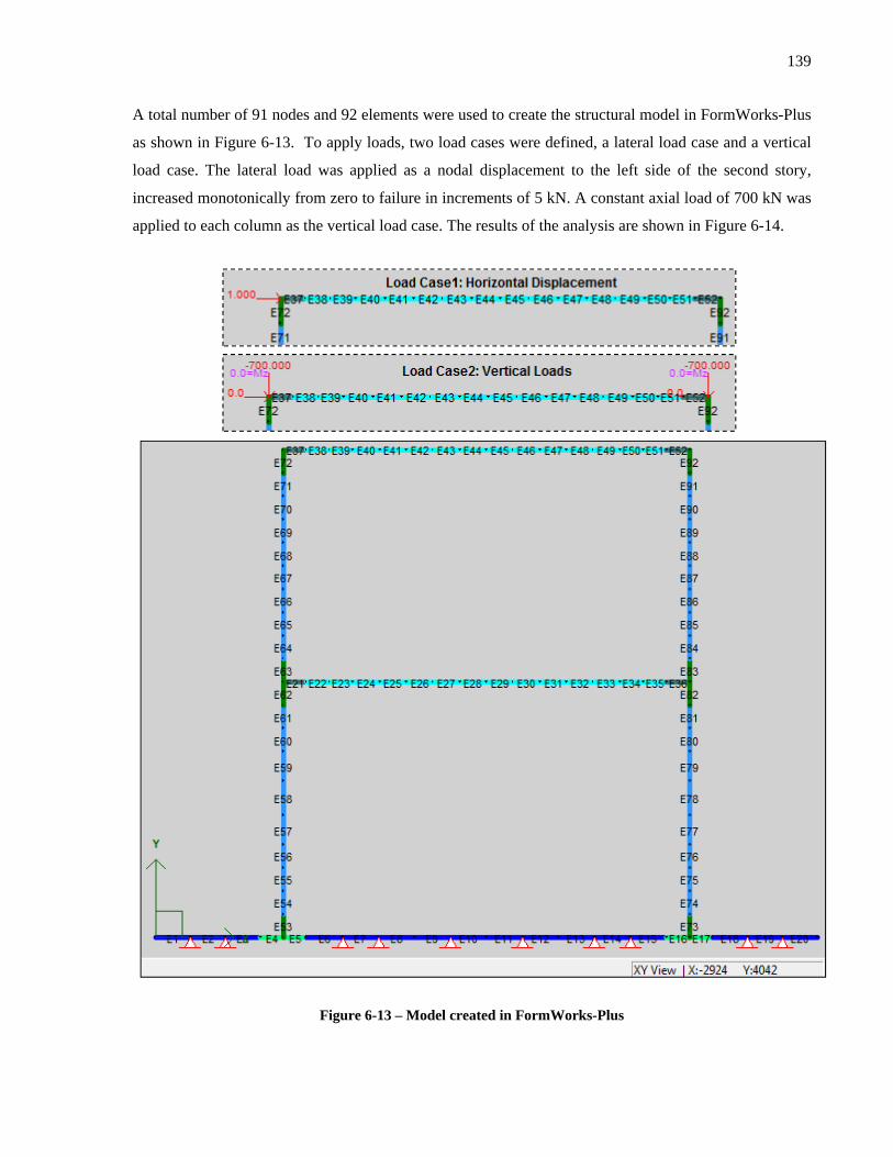
139

A total number of 91 nodes and 92 elements were used to create the structural model in FormWorks-Plus

as shown in Figure 6-13. To apply loads, two load cases were defined, a lateral load case and a vertical

load case. The lateral load was applied as a nodal displacement to the left side of the second story,

increased monotonically from zero to failure in increments of 5 kN. A constant axial load of 700 kN was

applied to each column as the vertical load case. The results of the analysis are shown in Figure 6-14.

Figure 6-13 – Model created in FormWorks-Plus

140

Material Type

General Properties

Concrete Properties Transverse Reinforcing Bars Properties

Colour F'c Ec e0 Other

Properties

St Dbt Fyz Fyt Fut Est eu esht

MPa MPa me mm mm MPa MPa MPa MPa me me

1 30 27386 2.025 default 125 11.3 454 454 640 200000 100 10

2 30 27386 2.025 default 125 11.3 454 454 640 200000 100 10

3 30 27386 2.025 default 200 11.3 454 454 640 200000 100 10

4 30 27386 2.025 default 125 11.3 454 454 640 200000 100 10

5 30 27386 2.025 default 125 11.3 454 454 640 200000 100 10

6 30 27386 2.025 default 200 11.3 454 454 640 200000 100 10

Table 6-1 (A) – Material properties defined in FormWorks-Plus – General properties

Concrete Layer Properties (from top of the section)

Type Colour Comp #

Dc Wc Rho‐t Rho‐z Nx Type Colour

Comp#

Dc Wc Rho‐t Rho‐z Nx

mm mm % % mm

mm % %

1

1 10 800 0 0.92 4

4

1 10 300 0 1.6 3

2 10 800 0.25 0.92 2 2 10 300 1.066 1.6 2

3 10 800 0.25 0.92 5 3 10 300 1.066 1.6 5

4 10 800 0.25 0 18 4 10 300 1.066 0 20

5 10 800 0.25 0.92 5 5 10 300 1.066 1.6 5

6 10 800 0.25 0.92 2 6 10 300 1.066 1.6 2

7 10 800 0 0.92 4 7 10 300 0 1.6 3

2

1 10 300 0 0.89 2

5

1 10 300 0 1.78 2

2 10 300 0.533 0.89 2 2 10 300 1.066 1.78 2

3 10 300 0.533 0.89 5 3 10 300 1.066 1.78 5

4 10 300 0.533 0 22 4 10 300 1.066 0 22

5 10 300 0.533 0.89 5 5 10 300 1.066 1.78 5

6 10 300 0.533 0.89 2 6 10 300 1.066 1.78 2

7 10 300 0 0.89 2 7 10 300 0 1.78 2

3

1 10 800 0 0.46 4

6

1 10 800 0 0.92 4

2 10 800 0.125 0.46 2 2 10 800 0.25 0.92 2

3 10 800 0.125 0.46 5 3 10 800 0.25 0.92 5

4 10 800 0.125 0 18 4 10 800 0.25 0 18

5 10 800 0.125 0.46 5 5 10 800 0.25 0.92 5

6 10 800 0.125 0.46 2 6 10 800 0.25 0.92 2

7 10 800 0 0.46 4 7 10 800 0 0.92 4

Table 6-1 (B) – Material properties defined in FormWorks-Plus – Concrete layer properties

141

Longitudinal Reinforcing Bar Layer Properties (from top of the section)

Type Colour Comp #

Ys As Db Fy Fu Es eu esh

mm mm^2 mm MPa MPa MPa me me

1 1 50 1200 19.5 418 596 200000 100 10

2 350 1200 19.5 418 596 200000 100 10

2 1 40 1200 19.5 418 596 200000 100 10

2 360 1200 19.5 418 596 200000 100 10

3 1 60 3000 19.5 418 596 200000 100 10

2 340 3300 19.5 418 596 200000 100 10

4 1 50 2400 19.5 418 596 200000 100 10

2 350 2400 19.5 418 596 200000 100 10

5 1 40 2400 19.5 418 596 200000 100 10

2 360 2400 19.5 418 596 200000 100 10

6 1 60 6000 19.5 418 596 200000 100 10

2 340 6600 19.5 418 596 200000 100 10

Table 6-1 (C) – Material properties defined in FormWorks-Plus – Reinforcement layer properties

Figure 6-14– Deformed shape of structure

142

Chapter 7

Summary and Recommendations

7.1 Summary

The VecTor(c) suite of programs has been developed at the University of Toronto for nonlinear analysis

of reinforced concrete structures. A graphics-based pre-processor, FormWorks, previously developed for

use specifically with VecTor2, greatly facilitates the modeling process of 2D Membrane Structures.

However, a user-friendly pre-processor is required for the entire suite of programs if they are to be of

greater use by potential users.

The first objective of this thesis was to develop an updated version of FormWorks, FormWorks 3.5,

which is more user-friendly and compatible with newer versions of VecTor2. The second objective was

to create a new version of FormWorks, FormWorks-Plus, capable of modeling different types of

structures including 2D Membrane Structures, 3D Solid Structures, Shell Structures, Plane Frame

Structures, and Axisymmetric Solid Structures.

FormWorks 3.5 was mainly developed to model the different types of materials now available in

VecTor2 including Reinforced Concrete, Structural Steel, Masonry, Wood, Concrete-Steel Laminate,

Concrete-SFRC Laminate, Masonry-SFRC Laminate, Concrete-Ortho Laminate, Reinforcement, and

Bond. In addition, the Job Page was updated with the most recent behavioural models and analysis

parameters. The zooming feature of FormWorks was improved to display the geometry of the finite

element model properly. A new load type, Nodal Thermal Load, was added to the program allowing the

user to define thermal loads for nodes. The performance of the truss and rectangular elements was

improved. Finally, updated dialog boxes for nodes, elements, restraints, and load types were added to

facilitate the modifying process of finite element model.

FormWorks-Plus is a new version of FormWorks, compatible with entire suite of VecTor programs. In

addition to the XY, XZ, and ZY plane views, sectional and projection views were added to the program,

greatly contributing to its utility. FormWorks-Plus also uses a supporting program called 3D View which

is written with the MFC library and OpenGL (Open Graphics Library), allowing the user to see a 3D

view of the structural model. In addition, four different types of node coordinate definitions, five types of

elements, several load types, and new material properties are added to the software, making it compatible

with the remaining VecTor programs.

143

7.2 Recommendations

The following is a list of features and options that can be added to FormWorks-Plus to improve the

program’s performance and facilitate the modeling process:

In the current version of FormWorks-Plus, nodes and elements must be defined manually using

the increment feature which gives complete control over the mesh topology, but may be time

consuming for complicated geometries. Having an automatic meshing feature or using

predefined structures such as beams, columns, slabs, silos, tanks, and frames would allow easier

redefinition or refinement of the mesh and save much time.

Most graphical-based programs have Undo (reverses the last action performed) and Redo

(undoes the last Undo action) features allowing the user to easily correct mistakes. Work needs

to be done to add these useful features to the program.

In order to find node coordinates for modeling complex structures, the user is required to draw

the model in another program like AutoCAD and then add them in FormWorks-Plus manually.

To avoid this time consuming process, an Insert feature can be added to the program to import

node coordinates, created by a drawing software, from a text file.

Defining sectional properties including concrete and reinforcing bar layers for Plane Frame

Structures is complicated and requires an expert user with a good understanding of VecTor5.

Another method that could be implemented to define sections only based on general properties

and compute remaining material parameters automatically.

The addition of a help option which provides a description of each part of the program would be

beneficial.

The current version of FormWorks-Plus is only capable of displaying the 3D view of a structural

model. It would be useful to be able to modify the finite element model such that specifying

loads, assigning material types, and redefining the mesh could be done in 3D view as well.

Works need to be done to improve the displaying capabilities of the program for element loads.

For instance, for uniformly distributed loads or pressure loads it would be more useful to display

the load pattern with arrows or colour contours instead of just numbers on the elements.

Different versions of FormWorks use different file extensions to save and open files. Previous

versions of FormWorks stored data as a *.fws file. FormWorks 3.5 saves files with a *.fwk

144

extension and finally FormWorks-Plus uses a *.fwp extension. Using different file extensions

makes it easier for the user to recognize which version of FormWorks was used to create the file.

It would be beneficial to make the program capable of opening all these file extensions.

145

References

Bazant, Z. P. (2002), “Concrete Fracture Models: Testing and Practice,” Engineering Fracture

Mechanics, V. 69, pp 165-205.

Bonaldo, E., de Barros, J. A. O., and Lourenco, P. B. (2006), “Efficient Strengthening Technique for

Reinforced Concrete Slabs,” Measuring, Monitoring and Modeling Concrete Properties, pp 125-131.

CEB-FIP (2010), “Model Code 2010,” Comité EURO-International du Béton, Paris, V.1, 311 pp.

Collins, M. P. and Mitchell, D. (1997), “Prestressed Concrete Structures,” Response Publications, 766

pp.

Fanella, D. A. and Naaman, A. (1985), “Stress-Strain Properties of Fiber Reinforced Mortar in

Compression,” ACI Journal, 82 (4), pp 475-483.

Guner, S. (2008), “Performance Assessment of Shear-Critical Reinforced Concrete Plane Frames,” PhD.

Thesis, Department of Civil Engineering, University of Toronto, 464 pp.

Gutkowski, R. M., Balogh, J., and To, L. G. (2010), “Finite-Element Modeling of Short-Term Field

Response of Composite Wood-Concrete Floors/Decks,” Journal of Structural Engineering, pp 707-714.

Hasebe, K. and Usuki, S. (1987), “Application of Orthotropic Failure Criterion to Wood,” Journal of

Engineering Mechanics, Vol. 115, No. 4, pp 867-872.

Heiduschke, A. and Kasal, B. (2003), “Composite Cross Section with High Performance Fibre reinforced

Concrete and Timbre,” Forest Products Journal, V. 53, No. 10, pp 74-78.

Horton, I. (2008), “Beginning Visual C++ 2008,” Indiana: Wiley Publishing Inc., 1356 pp.

Lourenco, P. J. B. (1996), “Computational Strategies for Masonry Structures,” PhD. Thesis, Department

of Civil Engineering, University of Delft, 220 pp.

Mital, V. P., Masood, A., Ahmad, T., and Arif, M. (2008), “Failure of Overhead Water Tank in the State

of Uttar Pradesh in India - A Case Study,” First International Conference on Construction in Developing

Countries, Karachi, Pakistan.

Naaman, A. E. (2003), “Engineered Steel Fibers with Optimal Properties for Reinforcement of Cement

Composites,” Journal of Advanced Concrete Technology, V. 1, No. 3, pp 241-252.

146

Onsongo, W. (1978), “The Diagonal Compression Field Theory for Reinforced Concrete Beams

Subjected to Combined Torsion, Flexure and Axial Load,” PhD. Thesis, Department of Civil

Engineering, University of Toronto.

Palermo, D., Abdulridha, A., and Foo, S. (2011), “Super elastic SMA Reinforced Concrete Elements:

Applicability and Practicality,” fib Symposium, Session 2B-9, Prague.

Polak, M. A. (1992), “Nonlinear Analysis of Reinforced Concrete Shells,” PhD. Thesis, Department of

Civil Engineering, University of Toronto, 195 pp.

Prosise, J. (1999), “Programming Windows with MFC,” Washington: Microsoft Press.

Schlaich, J., Schäfer, K., and Jennewein, M. (1987), “Toward a Consistent Design of Structural

Concrete,” PCI Journal, Issue 32, pp 74-150.

Schlöglmann, K. H. (2004), “Structural Behaviour of Masonry Panels and their Rehabilitation Focussing

on Lifeline Structures Subjected to Seismic Loads,” Diploma Thesis, Institute for Structural Concrete,

Graz, 216 pp.

Segal, M. and Akeley, K. (2006), “The OpenGL Graphics System,” California: Silicon Graphics Inc.,

333 pp.

Selby, R. G. (1990), “Nonlinear Finite Element Analysis of Reinforced Concrete Solids,” M.A.Sc.


Seracino, R. (1995), “Towards Improving Nonlinear Analysis of Reinforced Concrete Shells,” M.A.Sc.


Vecchio, F. J. (2000), “Disturbed Stress Field Model for Reinforced Concrete: Formulation,” Journal of

Structural Engineering, V.126, No.9, pp 1070-1077.

Vecchio, F. J. and Collins, M. P. (1986), “The Modified Compression-Field Theory for Reinforced

Concrete Elements Subjected to Shear,” ACI Journal, V.83, No.2, pp 219-231.

Vecchio, F. J. and Emara, M. B. (1992), “Shear Deformations in Reinforced Concrete Frames,” ACI

Structural Journal, pp 46-56.

147

Vecchio, F. J. and McQuade, I. (2011), “Towards Improved Modelling of Steel-Concrete Composite

Wall Elements,” Nuclear Engineering and Design, 241, pp 2629-2642.

Vecchio, F. J. and Selby, R. G. (1990), “Toward Compression-Field Analysis of Reinforced Concrete

Solids,” Journal of Structural Engineering, V. 117, No. 6, pp 1740-1757.

Vecchio, F. J. and Zhou, C. E. (2004), “Nonlinear Finite Element Analysis of Reinforced Concrete

Structures Subjected to Transient Thermal Loads,” Computers and Concrete, V. 2, No. 6, pp 455-479.

Wong, P. (2002), “User Facilities for 2D Nonlinear Finite Element Analysis of Reinforced Concrete,”

M.A.Sc. Thesis, Department of Civil Engineering, University of Toronto, 213 pp.

formworks-plus: improved pre-processor for vector analysis software

Documents