Formulations for Analysis of Probe-Fed

Printed Antennas in SuperNEC

Mmamolatelo E. Mathekga

A dissertation submitted to the Faculty of Engineering and the Built Environment, University of the

Witwatersrand, Johannesburg, in fulfilment of the requirements for the degree of Master of Science in

Engineering.

Johannesburg, 2008

i

Declaration

I declare that this dissertation is my own, unaided work, except where otherwise acknowledged. It is being

submitted for the degree of Master of Science in Engineering in the University of the Witwatersrand,

Johannesburg. It has not been submitted before for any degree or examination in any other university.

Signed this day of 20

Mmamolatelo E. Mathekga

ii

Dedicated to my mother - Ms. N.T. Mathekga

iii

Abstract

Formulations for analysis of printed antenna structures are derived and compared, to determine one to

implemented in SuperNEC based on the efficiency of its numerical solution in terms of memory usage and

solution time. SuperNEC is a software application for computing the response of electromagnetic structures

to electromagnetic fields. SuperNEC cannot be used for simulation of printed antenna structures. This is

because the formulation that is implemented in SuperNEC does not account for the effect of the substrates

that the radiating elements of the antenna structure are printed on, and it is also not intended for antenna

structures whose radiating elements are surfaces. Two MoM (Method of Moments) formulations and a FEM

(Finite Element Method)-MoM formulation are presented, together with different models for the antenna

feed. The FEM-MoM formulation is selected for implementation in SuperNEC because it is argued that it

is likely to be more memory efficient when compared to the MoM formulations, and also that less time

is required to fill the matrices resulting from the numerical solution of the formulation. The formulation

is implemented in a stand alone software application, which will be integrated into SuperNEC. Numerical

results that are computed using the software application are presented to illustrate correct implementation of

the formulation. The results are compared to: an exact solution, results from another publication, and results

computed using a different formulation. Good agreement is obtained in each case.

iv

Acknowledgements

I would like to extend my acknowledgements to my family particularly my mother. Your constant support -

financial or otherwise - is really appreciated and it is what kept me going. Thank you and God bless.

I would also like to thank Prof. A.R. Clark for the discussions, advice and trust. But more importantly I

would like to say thank you for letting me do it my way.

I also like to thank the people at Poynting for their help.

And, Heather Fraser. The Electromagnetics Laboratory would have been a dull place without you.

v

Preface

This dissertation is presented to the University of the Witwatersrand, Johannesburg for the degree of Master

of Science in Engineering.

The dissertation is entitled Formulations for Analysis of Probe-Fed Printed Antennas in SuperNEC. The

derivation of three formulations that can be used for analysis of probe-fed printed antennas are presented,

with various models for the antenna feed. One of the formulations is chosen for implementation in SuperNEC

based on the efficiency of its numerical solution in terms of memory usage and solution time. The chosen

formulation is implemented as a stand alone software application, which will be integrated into SuperNEC

and numerical results that were computed using the software application are presented.

This document complies with the university’s paper model format. The paper contains the main results of

the research. The appendices present in detail the work conducted during the research.

Appendix A presents:� Detailed derivation of the three formulations, which can be used for the analysis of probe-fed printed

antenna structures.� Discussion on the choice of the formulation of the formulation to be implemented in SuperNEC.

Appendix B presents the numerical results computed using the software application, which implements the

FEM-MoM formulation.

Appendix C presents the application of MoM for reducing the MoM formulation part of the FEM-MoM

formulation into a matrix equation.

Appendix D presents the application of FEM for reducing the FEM formulation part of the FEM-MoM

formulation into a matrix equation.

Appendix E presents the procedure for solving the matrix equations, which were derived in appendices B

and C.

Appendix F is the user manual of the software application that was developed to implement the FEM-MoM

formulation.

vi

Contents

Declaration i

Abstract iii

Acknowledgements iv

Preface v

Contents vi

List of Figures xii

List of Tables xiv

I Introduction . . . . . . . . . . . . . . . . . . . . . . . . . . . . . . . . . . . . . . . . . . . 1

II Formulations . . . . . . . . . . . . . . . . . . . . . . . . . . . . . . . . . . . . . . . . . . . 2

III MoM Formulations . . . . . . . . . . . . . . . . . . . . . . . . . . . . . . . . . . . . . . . 2

III-A Field Scattered by Conducting Surfaces . . . . . . . . . . . . . . . . . . . . . . . . 3

III-B Fields Scattered by Substrate . . . . . . . . . . . . . . . . . . . . . . . . . . . . . . 3

III-B1 Using the Volume Equivalence Principle . . . . . . . . . . . . . . . . . . 3

III-B2 Using the Surface Equivalence Principle . . . . . . . . . . . . . . . . . . 3

III-C Integral Equations . . . . . . . . . . . . . . . . . . . . . . . . . . . . . . . . . . . . 4

III-C1 Using the Volume Equivalence Principle . . . . . . . . . . . . . . . . . . 4

III-C2 Using the Surface Equivalence Principle . . . . . . . . . . . . . . . . . . 4

IV FEM-MoM Formulation . . . . . . . . . . . . . . . . . . . . . . . . . . . . . . . . . . . . . 4

IV-A FEM Formulation . . . . . . . . . . . . . . . . . . . . . . . . . . . . . . . . . . . . 5

IV-B MoM Formulation . . . . . . . . . . . . . . . . . . . . . . . . . . . . . . . . . . . 5

V Feed Model . . . . . . . . . . . . . . . . . . . . . . . . . . . . . . . . . . . . . . . . . . . 5

vii

V-A Magnetic Frill Generator . . . . . . . . . . . . . . . . . . . . . . . . . . . . . . . . 5

V-A1 Use with the MoM Formulation . . . . . . . . . . . . . . . . . . . . . . . 5

V-A2 Use with the FEM Formulation . . . . . . . . . . . . . . . . . . . . . . . 6

V-B Delta Gap Model . . . . . . . . . . . . . . . . . . . . . . . . . . . . . . . . . . . . 6

V-B1 Use with the MoM Formulation . . . . . . . . . . . . . . . . . . . . . . . 6

V-B2 Use with the FEM Formulation . . . . . . . . . . . . . . . . . . . . . . . 6

V-C Probe Feed Model . . . . . . . . . . . . . . . . . . . . . . . . . . . . . . . . . . . 6

VI Choice of Formulation . . . . . . . . . . . . . . . . . . . . . . . . . . . . . . . . . . . . . 6

VI-A Numerical Implementation . . . . . . . . . . . . . . . . . . . . . . . . . . . . . . . 7

VI-B Numerical Results . . . . . . . . . . . . . . . . . . . . . . . . . . . . . . . . . . . 7

VII Conclusion . . . . . . . . . . . . . . . . . . . . . . . . . . . . . . . . . . . . . . . . . . . . 7

References . . . . . . . . . . . . . . . . . . . . . . . . . . . . . . . . . . . . . . . . . . . . . . . 8

A Derivation of the Formulations for Radiation of Probe-Fed Printed Antennas A.1

A.1 Introduction . . . . . . . . . . . . . . . . . . . . . . . . . . . . . . . . . . . . . . . . . . . A.1

A.2 MoM Formulations . . . . . . . . . . . . . . . . . . . . . . . . . . . . . . . . . . . . . . . A.2

A.2.1 Fields Scattered by the Conducting Surface . . . . . . . . . . . . . . . . . . . . . . A.2

A.2.2 Fields Scattered by the Substrate . . . . . . . . . . . . . . . . . . . . . . . . . . . . A.4

A.2.2.1 Using the Volume Equivalence Principle . . . . . . . . . . . . . . . . . . A.4

A.2.2.2 Using the Surface Equivalence Principle . . . . . . . . . . . . . . . . . . A.4

A.2.3 Integral Equations . . . . . . . . . . . . . . . . . . . . . . . . . . . . . . . . . . . . A.6

A.2.3.1 Using the Volume Equivalence Principle . . . . . . . . . . . . . . . . . . A.6

A.2.3.2 Using the Surface Equivalence Principle . . . . . . . . . . . . . . . . . . A.7

A.2.4 Discussion . . . . . . . . . . . . . . . . . . . . . . . . . . . . . . . . . . . . . . . . A.7

A.3 FEM-MoM Formulation . . . . . . . . . . . . . . . . . . . . . . . . . . . . . . . . . . . . . A.8

A.3.1 FEM Formulation . . . . . . . . . . . . . . . . . . . . . . . . . . . . . . . . . . . . A.9

A.3.2 MoM Formulation . . . . . . . . . . . . . . . . . . . . . . . . . . . . . . . . . . . A.10

A.3.3 Discussion . . . . . . . . . . . . . . . . . . . . . . . . . . . . . . . . . . . . . . . . A.10

A.4 Feed Model . . . . . . . . . . . . . . . . . . . . . . . . . . . . . . . . . . . . . . . . . . . A.10

A.4.1 Magnetic Frill Generator . . . . . . . . . . . . . . . . . . . . . . . . . . . . . . . . A.11

viii

A.4.1.1 Use with the MoM Formulation . . . . . . . . . . . . . . . . . . . . . . . A.11

A.4.1.2 Use with the FEM Formulation . . . . . . . . . . . . . . . . . . . . . . . A.12

A.4.2 Delta Gap Model . . . . . . . . . . . . . . . . . . . . . . . . . . . . . . . . . . . . A.12

A.4.2.1 Use with the MoM Formulation . . . . . . . . . . . . . . . . . . . . . . . A.12

A.4.2.2 Use with the FEM Formulation . . . . . . . . . . . . . . . . . . . . . . . A.12

A.4.3 Probe Feed Model . . . . . . . . . . . . . . . . . . . . . . . . . . . . . . . . . . . A.12

A.5 Choice of Formulation . . . . . . . . . . . . . . . . . . . . . . . . . . . . . . . . . . . . . A.13

A.5.1 Memory Usage . . . . . . . . . . . . . . . . . . . . . . . . . . . . . . . . . . . . . A.14

A.5.1.1 Storage of Matrices . . . . . . . . . . . . . . . . . . . . . . . . . . . . . A.14

A.5.1.2 Solution of Matrix Equations . . . . . . . . . . . . . . . . . . . . . . . . A.15

A.5.2 Solution Time . . . . . . . . . . . . . . . . . . . . . . . . . . . . . . . . . . . . . . A.16

A.5.2.1 Matrix Fill Time . . . . . . . . . . . . . . . . . . . . . . . . . . . . . . . A.16

A.5.2.2 Matrix Solution Time . . . . . . . . . . . . . . . . . . . . . . . . . . . . A.16

A.5.3 Discussion . . . . . . . . . . . . . . . . . . . . . . . . . . . . . . . . . . . . . . . . A.17

A.6 Conclusion . . . . . . . . . . . . . . . . . . . . . . . . . . . . . . . . . . . . . . . . . . . . A.17

References . . . . . . . . . . . . . . . . . . . . . . . . . . . . . . . . . . . . . . . . . . . . . . . A.17

B Numerical Results B.1

B.1 Introduction . . . . . . . . . . . . . . . . . . . . . . . . . . . . . . . . . . . . . . . . . . . B.1

B.2 Radar Cross Section of PEC Sphere . . . . . . . . . . . . . . . . . . . . . . . . . . . . . . B.1

B.2.1 Monostatic Radar Cross Section . . . . . . . . . . . . . . . . . . . . . . . . . . . . B.2

B.2.2 Bistatic Radar Cross Section . . . . . . . . . . . . . . . . . . . . . . . . . . . . . . B.2

B.3 Printed Antenna Impedance . . . . . . . . . . . . . . . . . . . . . . . . . . . . . . . . . . . B.2

B.4 Conclusion . . . . . . . . . . . . . . . . . . . . . . . . . . . . . . . . . . . . . . . . . . . . B.6

References . . . . . . . . . . . . . . . . . . . . . . . . . . . . . . . . . . . . . . . . . . . . . . . B.6

C Reduction of MoM Formulation into a Matrix Equation C.1

C.1 Introduction . . . . . . . . . . . . . . . . . . . . . . . . . . . . . . . . . . . . . . . . . . . C.1

C.2 MoM Formulation . . . . . . . . . . . . . . . . . . . . . . . . . . . . . . . . . . . . . . . . C.2

C.3 Overview of the Method of Moments . . . . . . . . . . . . . . . . . . . . . . . . . . . . . C.2

ix

C.4 Basis and Testing Functions . . . . . . . . . . . . . . . . . . . . . . . . . . . . . . . . . . C.3

C.4.1 Basis Functions . . . . . . . . . . . . . . . . . . . . . . . . . . . . . . . . . . . . . C.3

C.4.2 Testing Functions . . . . . . . . . . . . . . . . . . . . . . . . . . . . . . . . . . . . C.5

C.5 Formulation of System Matrices . . . . . . . . . . . . . . . . . . . . . . . . . . . . . . . . C.5

C.6 Evaluation of the Integrals . . . . . . . . . . . . . . . . . . . . . . . . . . . . . . . . . . . C.6

C.6.1 Evaluation of I1 . . . . . . . . . . . . . . . . . . . . . . . . . . . . . . . . . . . . . C.7

C.6.1.1 Testing with RWG Function . . . . . . . . . . . . . . . . . . . . . . . . . C.7

C.6.1.2 Testing with n�RWG Function . . . . . . . . . . . . . . . . . . . . . . . C.9

C.6.2 Evaluation of I2 . . . . . . . . . . . . . . . . . . . . . . . . . . . . . . . . . . . . . C.10

C.6.3 Evaluation of I3 . . . . . . . . . . . . . . . . . . . . . . . . . . . . . . . . . . . . . C.10

C.6.3.1 Testing with RWG Function . . . . . . . . . . . . . . . . . . . . . . . . . C.11

C.6.3.2 Testing with n�RWG Function . . . . . . . . . . . . . . . . . . . . . . . C.13

C.6.4 Numerical Integration . . . . . . . . . . . . . . . . . . . . . . . . . . . . . . . . . . C.14

C.6.4.1 Line Integrals . . . . . . . . . . . . . . . . . . . . . . . . . . . . . . . . . C.14

C.6.4.2 Surface Integrals . . . . . . . . . . . . . . . . . . . . . . . . . . . . . . . C.17

C.7 Conclusion . . . . . . . . . . . . . . . . . . . . . . . . . . . . . . . . . . . . . . . . . . . . C.18

References . . . . . . . . . . . . . . . . . . . . . . . . . . . . . . . . . . . . . . . . . . . . . . . C.18

D Reduction of FEM Formulation into a Matrix Equation D.1

D.1 Introduction . . . . . . . . . . . . . . . . . . . . . . . . . . . . . . . . . . . . . . . . . . . D.1

D.2 Formulation . . . . . . . . . . . . . . . . . . . . . . . . . . . . . . . . . . . . . . . . . . . D.2

D.3 Overview of the Finite Element Method . . . . . . . . . . . . . . . . . . . . . . . . . . . . D.2

D.4 Domain Discretisation . . . . . . . . . . . . . . . . . . . . . . . . . . . . . . . . . . . . . . D.3

D.5 Selection of Interpolation Functions . . . . . . . . . . . . . . . . . . . . . . . . . . . . . . D.4

D.5.0.3 Simplex Coordinates . . . . . . . . . . . . . . . . . . . . . . . . . . . . . D.5

D.6 Formulation of the System Matrices . . . . . . . . . . . . . . . . . . . . . . . . . . . . . . D.7

D.7 Evaluation of Integrals . . . . . . . . . . . . . . . . . . . . . . . . . . . . . . . . . . . . . D.7

D.7.1 Volume Integrals . . . . . . . . . . . . . . . . . . . . . . . . . . . . . . . . . . . . D.7

D.7.2 Surface Integral . . . . . . . . . . . . . . . . . . . . . . . . . . . . . . . . . . . . . D.9

D.8 Conclusion . . . . . . . . . . . . . . . . . . . . . . . . . . . . . . . . . . . . . . . . . . . . D.10

x

References . . . . . . . . . . . . . . . . . . . . . . . . . . . . . . . . . . . . . . . . . . . . . . . D.11

E Solution of Matrix Equations E.1

References . . . . . . . . . . . . . . . . . . . . . . . . . . . . . . . . . . . . . . . . . . . . . . . E.2

F fmsolver User Manual F.1

F.1 Introduction . . . . . . . . . . . . . . . . . . . . . . . . . . . . . . . . . . . . . . . . . . . F.1

F.2 Program Input and Output . . . . . . . . . . . . . . . . . . . . . . . . . . . . . . . . . . . F.2

F.2.1 Mesh File . . . . . . . . . . . . . . . . . . . . . . . . . . . . . . . . . . . . . . . . F.2

F.2.1.1 Continous Conducting Surfaces . . . . . . . . . . . . . . . . . . . . . . . F.4

F.2.1.2 Dielectric Volumes . . . . . . . . . . . . . . . . . . . . . . . . . . . . . . F.4

F.2.1.3 Probe-Fed Printed Antenna Structure . . . . . . . . . . . . . . . . . . . . F.5

F.2.2 Input File . . . . . . . . . . . . . . . . . . . . . . . . . . . . . . . . . . . . . . . . F.6

F.2.2.1 Problem Data . . . . . . . . . . . . . . . . . . . . . . . . . . . . . . . . . F.6

F.2.2.2 Geometry Data . . . . . . . . . . . . . . . . . . . . . . . . . . . . . . . . F.7

F.2.2.3 Analysis Request . . . . . . . . . . . . . . . . . . . . . . . . . . . . . . . F.7

F.2.3 Output File . . . . . . . . . . . . . . . . . . . . . . . . . . . . . . . . . . . . . . . F.8

F.3 Commands . . . . . . . . . . . . . . . . . . . . . . . . . . . . . . . . . . . . . . . . . . . . F.8

F.3.1 MFP Command . . . . . . . . . . . . . . . . . . . . . . . . . . . . . . . . . . . . . F.8

F.3.2 STR Command . . . . . . . . . . . . . . . . . . . . . . . . . . . . . . . . . . . . . F.8

F.3.2.1 Conducting Surface . . . . . . . . . . . . . . . . . . . . . . . . . . . . . F.9

F.3.2.2 Probe-Fed Printed Antenna . . . . . . . . . . . . . . . . . . . . . . . . . F.9

F.3.2.3 Dielectric Volume . . . . . . . . . . . . . . . . . . . . . . . . . . . . . . F.10

F.3.3 EX Command . . . . . . . . . . . . . . . . . . . . . . . . . . . . . . . . . . . . . . F.10

F.3.3.1 Plane Wave . . . . . . . . . . . . . . . . . . . . . . . . . . . . . . . . . . F.10

F.3.3.2 Probe Feed . . . . . . . . . . . . . . . . . . . . . . . . . . . . . . . . . . F.11

F.3.3.3 No Excitation . . . . . . . . . . . . . . . . . . . . . . . . . . . . . . . . . F.12

F.3.4 FR Command . . . . . . . . . . . . . . . . . . . . . . . . . . . . . . . . . . . . . . F.12

F.3.5 DE Command . . . . . . . . . . . . . . . . . . . . . . . . . . . . . . . . . . . . . . F.12

F.3.6 FS Command . . . . . . . . . . . . . . . . . . . . . . . . . . . . . . . . . . . . . . F.13

xi

F.3.7 NF Command . . . . . . . . . . . . . . . . . . . . . . . . . . . . . . . . . . . . . . F.13

F.3.8 FP Command . . . . . . . . . . . . . . . . . . . . . . . . . . . . . . . . . . . . . . F.13

F.3.9 CD Command . . . . . . . . . . . . . . . . . . . . . . . . . . . . . . . . . . . . . . F.14

F.3.10 EF Command . . . . . . . . . . . . . . . . . . . . . . . . . . . . . . . . . . . . . . F.15

F.4 Error Messages . . . . . . . . . . . . . . . . . . . . . . . . . . . . . . . . . . . . . . . . . F.15

F.5 Example Input File . . . . . . . . . . . . . . . . . . . . . . . . . . . . . . . . . . . . . . . F.15

References . . . . . . . . . . . . . . . . . . . . . . . . . . . . . . . . . . . . . . . . . . . . . . . F.16

xii

List of Figures

1 Example probe fed printed antenna. . . . . . . . . . . . . . . . . . . . . . . . . . . . . . . 2

2 Substrate (a) with outer (b) and inner (c) equivalent problems. . . . . . . . . . . . . . . . . 3

3 Cross-section of a probe-fed printed antenna without substrate (a) and the feed opening (b). 5

4 Positions of the current filaments (solid black lines) using the strip model. . . . . . . . . . 6

5 Geometry of patch antenna with dimensions. . . . . . . . . . . . . . . . . . . . . . . . . . 7

6 Reactance of patch antenna as a function of frequency. . . . . . . . . . . . . . . . . . . . . 7

7 Impedance magnitude as a function of frequency. . . . . . . . . . . . . . . . . . . . . . . . 8

8 Reactance of patch antennas as a function of frequency for a fine and coarse meshes. . . . 8

A.1 Example probe fed printed antenna. . . . . . . . . . . . . . . . . . . . . . . . . . . . . . . A.1

A.2 PEC Conductor (a) and equivalent problem (b). . . . . . . . . . . . . . . . . . . . . . . . . A.3

A.3 Substrate (a) with outer (b) and inner (c) equivalent problems. . . . . . . . . . . . . . . . . A.5

A.4 Arbitrary printed antenna structure (a) with inner (b) and outer (c) equivalent problems. . . A.9

A.5 Cross-section of a probe-fed printed antenna without substrate (a) and the feed opening (b). A.11

A.6 Positions of the current filaments (solid black lines) using the strip model. . . . . . . . . . A.13

B.1 PEC sphere illuminated by plane wave. . . . . . . . . . . . . . . . . . . . . . . . . . . . . B.2

B.2 Monostatic RCS of a PEC sphere. . . . . . . . . . . . . . . . . . . . . . . . . . . . . . . . B.3

B.3 Coated PEC sphere illuminated by a plane wave. . . . . . . . . . . . . . . . . . . . . . . . B.3

B.4 Bistatic RCS of PEC sphere of radius 0.3367 m for � = 00 and 00 � �1800 . . . . . . . . . B.4

B.5 Geometry of patch antenna structure with dimensions. . . . . . . . . . . . . . . . . . . . . B.4

B.6 Reactance of the patch antenna as a function of frequency. . . . . . . . . . . . . . . . . . . B.5

B.7 Impedance magnitude as a function of frequency. . . . . . . . . . . . . . . . . . . . . . . . B.5

B.8 Results for a coarse and fine mesh of the antenna structure. . . . . . . . . . . . . . . . . . B.6

C.1 Triangles with parameters related to the definition of the RWG basis function. . . . . . . . C.4

C.2 Triangular domain with definition of variables used for evaluation of the integrals. . . . . . C.9

xiii

C.3 Triangle in different coordinate systems. . . . . . . . . . . . . . . . . . . . . . . . . . . . . C.16

D.1 Enumeration of the edges, and nodes for a triangle and tetrahedron. . . . . . . . . . . . . . D.4

D.2 Triangle. . . . . . . . . . . . . . . . . . . . . . . . . . . . . . . . . . . . . . . . . . . . . . D.5

D.3 Tetrahedron. . . . . . . . . . . . . . . . . . . . . . . . . . . . . . . . . . . . . . . . . . . . D.6

F.1 Cross-section of the volumetric region where the electric field distribution is computed. . . F.1

F.2 Continuos surface (a), and surface with a branch (b). . . . . . . . . . . . . . . . . . . . . . F.3

F.3 Triangle (b) and Tetrahedron (b) with node definitions. . . . . . . . . . . . . . . . . . . . . F.3

F.4 Example probe-fed printed antenna structure. . . . . . . . . . . . . . . . . . . . . . . . . . F.5

F.5 Surface with details of the front and back views of the antenna structure in figure F.4. . . . F.5

F.6 Open surface with four reference points. . . . . . . . . . . . . . . . . . . . . . . . . . . . . F.9

xiv

List of Tables

A.1 Matrices generated for the different formulations. . . . . . . . . . . . . . . . . . . . . . . . . A.14

C.1 Weights and points for the 3-point Gaussian-Legendre integration rule. . . . . . . . . . . . . . C.14

C.2 Weights and points for the 7-point Gaussian quadrature rule. . . . . . . . . . . . . . . . . . . C.17

F.1 Format of the input file . . . . . . . . . . . . . . . . . . . . . . . . . . . . . . . . . . . . . . F.6

F.2 Commands for the problem data section of input file . . . . . . . . . . . . . . . . . . . . . . F.7

F.3 Commands for specifying additional information about the mesh elements. . . . . . . . . . . . F.7

F.4 Commands for specifying additional information about the mesh elements. . . . . . . . . . . . F.8

F.5 Definition of the arguments of STR CS . . . command. . . . . . . . . . . . . . . . . . . . . . . F.9

F.6 Definition of the arguments of STR PA command . . . . . . . . . . . . . . . . . . . . . . . . . F.10

F.7 Excitation options for EX command . . . . . . . . . . . . . . . . . . . . . . . . . . . . . . . F.11

F.8 Definition of the arguments of EX 0 . . . command . . . . . . . . . . . . . . . . . . . . . . . . F.11

F.9 Definition of the arguments of EX 1 . . . command . . . . . . . . . . . . . . . . . . . . . . . . F.11

F.10 Definition of the arguments of FR . . . command . . . . . . . . . . . . . . . . . . . . . . . . . F.12

F.11 Definition of the arguments of DE . . . command . . . . . . . . . . . . . . . . . . . . . . . . . F.12

F.12 Coordinate system options for NF command . . . . . . . . . . . . . . . . . . . . . . . . . . . F.13

F.13 Definition of the arguments of NF command. . . . . . . . . . . . . . . . . . . . . . . . . . . F.14

F.14 Definition of the arguments of FP command. . . . . . . . . . . . . . . . . . . . . . . . . . . . F.14

Part 1

Paper: Formulations for Analysis of Probe-Fed

Printed Antennas in SuperNEC

1

Formulations for Analysis of Probe-Fed Printed Antennas in

SuperNEC

Mmamolatelo E. Mathekga

Abstract—Formulations for analysis of printed antenna structures are

derived and compared, to determine one to implemented in SuperNEC

based on the efficiency of its numerical solution in terms of memory usage

and solution time. SuperNEC is a software application for computing

the response of electromagnetic structures to electromagnetic fields.

SuperNEC cannot be used for simulation of printed antenna structures.

This is because the formulation that is implemented in SuperNEC does

not account for the effect of the substrates that the radiating elements

of the antenna structure are printed on, and it is also not intended

for antenna structures whose radiating elements are surfaces. Two MoM

(Method of Moments) formulations and a FEM (Finite Element Method)-

MoM formulation are presented, together with different models for the

antenna feed. The FEM-MoM formulation is selected for implementation

in SuperNEC because it is argued that it is likely to be more memory

efficient when compared to the MoM formulations, and also that less time

is required to fill the matrices resulting from the numerical solution of the

formulation. The formulation is implemented in a stand alone software

application, which will be integrated into SuperNEC. Input impedance

computed using the software application, for a probe-fed printed antenna

are presented and compared with results from a previous publication and

good agreement is obtained.

Index Terms—FEM, Formulation, MoM, Printed Antenna, Probe Feed

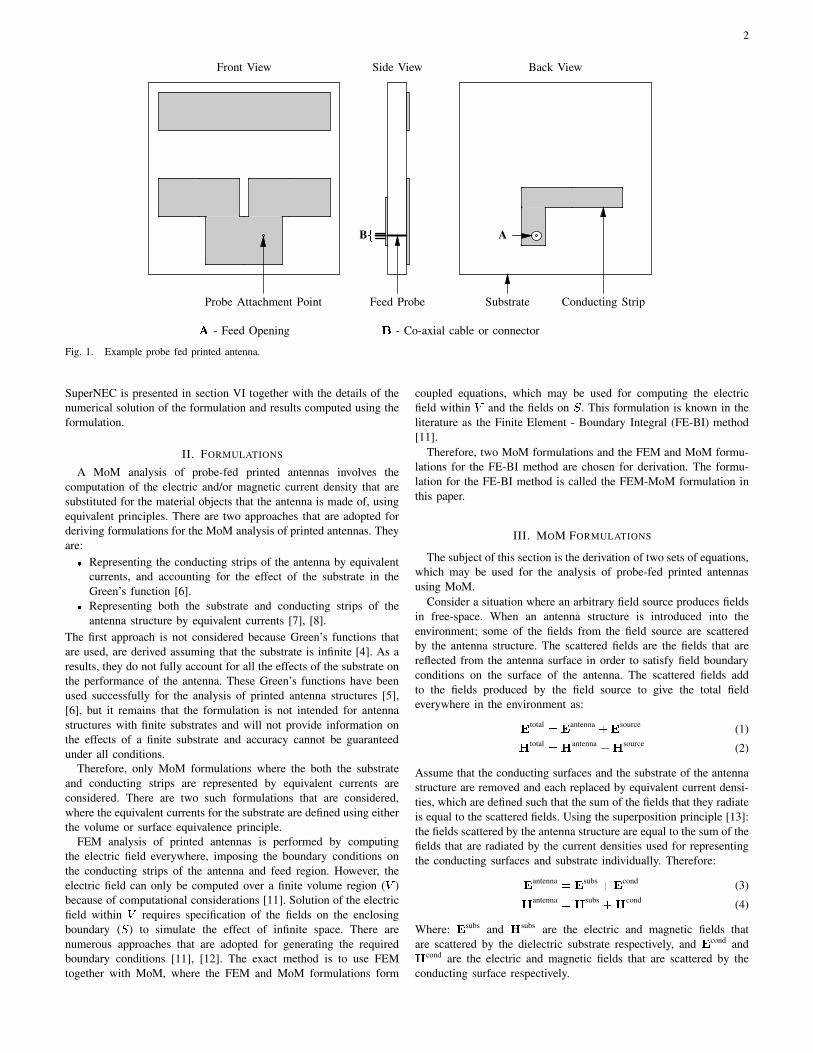
I. INTRODUCTION

THE use of higher frequencies for communication and the need

for miniaturisation, has made printed antennas the antennas of

choice. Printed antennas are antennas that are made from a conducting

strips bonded to a substrate as shown figure 1. The substrate and the

conducting strips may be shaped as necessary to meet the antenna

design requirements. The probe-feed is one of the methods that are

used for feeding these types of antennas, particularly when using a

coaxial cable to connect the antenna to the electronic device that it is

used with. It consists of a conducting wire (usually the inner wire of

a coaxial cable), which goes through a hole on one of the conducting

strips and connects to the other conducting surface on the opposite

side of the substrate. Fields from the cable enter the antenna through

the hole on one of the conducting surfaces. Details of the co-axial

feed can be seen in figure 1.

These antennas are popular because of their many advantages.

Some of the advantages are: low production costs, ability to conform

to surfaces, and they do not have protruding parts and are not

susceptible to breakage like wire antennas.

Simulation forms an integral part of design. This is because designs

have become so complex that creating a prototype is not feasible until

the design can be confirmed to some extent. Thus, the need arises

for more accurate simulation software to minimise development time

and cost, since an accurate simulation means a more accurate first

prototype.

SuperNEC is software application for computing the response

of electromagnetic structures to electromagnetic fields. It is a C++

implementation of the formulation of NEC-2 (Numerical Electro-

magnetics Code) [1] used for treating wire structures with a hybrid

MoM (Method of Moments) - UTD (Unified Theory of Diffraction)

solver. However, SuperNEC cannot be used for simulation of probe-

fed printed antenna structures with dielectric substrates. The reason

for this is that: the formulation implemented in SuperNEC is meant

for conducting wires radiating in free-space or in the presence of

other conducting structures [1].

SuperNEC is also unsuitable for analysis of probe-fed printed

antenna structures such as the one in figure 1. The reason for this

is that conducting strips of printed antennas are surfaces and not

wires. Therefore, simulation of these types of antennas in SuperNEC,

ignoring the fact that the effect of the substrate is not taken into

account; is performed by representing the conducting strips as a wire

grid.

The practice of modeling conducting surfaces as wire grids has

been used successfully by Richmond in [2] and satisfactory results

have been obtained for monostatic RCS (Radar Cross-Section) of

conducting plates and bodies of revolution. Guidelines for creating

wire grids that can be used for modeling conducting surfaces in NEC-

2 are presented in [1] and [3]. The wire grid model of a conducting

surface is found to be accurate for far field parameters but, its validity

for near field parameters cannot be confirmed [1].

The fact that accurate solutions have been obtained cannot be

denied. However, the formulation is not intended for modeling

conducting surfaces. Therefore, accurate results cannot be guaranteed,

especially when one considers that refining the wire grid does not

necessarily result in a more accurate solution as would be expected

[4, Chapter 5]. This is because of the thin-wire approximations that

are made in the derivation of the formulation. Therefore, a different

formulation is required for analysis of printed antennas in SuperNEC.

Analysis of printed antennas has been performed using MoM and

FEM (Finite Element Method) [5], [6], [7], [8], [9], [10] and different

formulations have been used with both numerical techniques. The

subject of this paper is the:� Selection of MoM and FEM formulations for use in SuperNEC.� Derivation of the selected formulations with different source

models for the feed.� Selection of one of the formulations for implementation in

SuperNEC based on the efficiency of its numerical solution in

terms of memory usage and solution time.� Presentation of the results computed using the selected formu-

lation.

The presentation in this paper is structured as follows. The different

formulations that can be used for analysis of probe-fed printed

antennas are presented and the ones that may be used in SuperNEC

are chosen in section II. Then, the derivation of the selected for-

mulation and models for the feed are presented in sections III, IV,

and V. The choice for the formulation that will be implemented in

2

Front View Side View Back View

SubstrateFeed ProbeProbe Attachment Point Conducting Strip

ABfA - Feed Opening B - Co-axial cable or connector

Fig. 1. Example probe fed printed antenna.

SuperNEC is presented in section VI together with the details of the

numerical solution of the formulation and results computed using the

formulation.

II. FORMULATIONS

A MoM analysis of probe-fed printed antennas involves the

computation of the electric and/or magnetic current density that are

substituted for the material objects that the antenna is made of, using

equivalent principles. There are two approaches that are adopted for

deriving formulations for the MoM analysis of printed antennas. They

are:� Representing the conducting strips of the antenna by equivalent

currents, and accounting for the effect of the substrate in the

Green’s function [6].� Representing both the substrate and conducting strips of the

antenna structure by equivalent currents [7], [8].

The first approach is not considered because Green’s functions that

are used, are derived assuming that the substrate is infinite [4]. As a

results, they do not fully account for all the effects of the substrate on

the performance of the antenna. These Green’s functions have been

used successfully for the analysis of printed antenna structures [5],

[6], but it remains that the formulation is not intended for antenna

structures with finite substrates and will not provide information on

the effects of a finite substrate and accuracy cannot be guaranteed

under all conditions.

Therefore, only MoM formulations where the both the substrate

and conducting strips are represented by equivalent currents are

considered. There are two such formulations that are considered,

where the equivalent currents for the substrate are defined using either

the volume or surface equivalence principle.

FEM analysis of printed antennas is performed by computing

the electric field everywhere, imposing the boundary conditions on

the conducting strips of the antenna and feed region. However, the

electric field can only be computed over a finite volume region (V )

because of computational considerations [11]. Solution of the electric

field within V requires specification of the fields on the enclosing

boundary (S) to simulate the effect of infinite space. There are

numerous approaches that are adopted for generating the required

boundary conditions [11], [12]. The exact method is to use FEM

together with MoM, where the FEM and MoM formulations form

coupled equations, which may be used for computing the electric

field within V and the fields on S. This formulation is known in the

literature as the Finite Element - Boundary Integral (FE-BI) method

[11].

Therefore, two MoM formulations and the FEM and MoM formu-

lations for the FE-BI method are chosen for derivation. The formu-

lation for the FE-BI method is called the FEM-MoM formulation in

this paper.

III. MOM FORMULATIONS

The subject of this section is the derivation of two sets of equations,

which may be used for the analysis of probe-fed printed antennas

using MoM.

Consider a situation where an arbitrary field source produces fields

in free-space. When an antenna structure is introduced into the

environment; some of the fields from the field source are scattered

by the antenna structure. The scattered fields are the fields that are

reflected from the antenna surface in order to satisfy field boundary

conditions on the surface of the antenna. The scattered fields add

to the fields produced by the field source to give the total field

everywhere in the environment as:Etotal = Eantenna +Esource(1)Htotal = Hantenna +Hsource(2)

Assume that the conducting surfaces and the substrate of the antenna

structure are removed and each replaced by equivalent current densi-

ties, which are defined such that the sum of the fields that they radiate

is equal to the scattered fields. Using the superposition principle [13]:

the fields scattered by the antenna structure are equal to the sum of the

fields that are radiated by the current densities used for representing

the conducting surfaces and substrate individually. Therefore:Eantenna = Esubs +Econd(3)Hantenna = Hsubs +Hcond(4)

Where: Esubs and Hsubs are the electric and magnetic fields that

are scattered by the dielectric substrate respectively, and Econd andHcond are the electric and magnetic fields that are scattered by the

conducting surface respectively.

3

A. Field Scattered by Conducting Surfaces

Using the surface equivalence principle with the field conditions

inside and on the boundary of the finite volume conductor, which

is assumed to be perfectly conducting: the conductor is represented

by equivalent electric current density on a closed fictitious surface,

which encloses the conductor and is chosen equal to the surface of

the conductor. Given that fields inside the conductor are equal to zero:

the conductor is removed and region inside the fictitious surface is

filled with free-space material.

This reduces the problem to an electric current density on the

fictitious surface radiating in free-space. The electric current density

is defined as: Jcondeq = n�Htotal

(5)

Where: n is the outward pointed unit normal on the surface of the

conductor, and Htotal is the magnetic field in free-space. Using the

notation from [11]: the fields that are scattered by the conductor are

given by: Econd = �Z0L(Jcondeq ) (6)Hcond = �K(Jcond

eq ) (7)L and K are operators, which are defined as:L(X) = jk0�SX(r0)G(r; r0)ds0+jk20 �S r0 �X(r0)rG(r; r0)ds0 (8)

And: K(X) = �SX(r0)�rG(r; r0)ds0 (9)

Where:� G(r; r0) = e�jkjr�r0j=4�jr � r0j, is the free-space Green’s

function� Z0 =p�0=�0 is the wave impedance of free-space.� k = 2�=� is the wavenumber.� S is the surface over which X is defined.� r and r0 are the position vectors everywhere in the environment

and on S respectively.

The above derivation may also be applied for computing the fields

that are scattered by a real conductor. Fields in a real conductor

are confined to a thin layer on the surface at high frequencies. The

conductivity value of conductors are large enough that the tangential

electric field can be assumed to be negligible.

B. Fields Scattered by Substrate

Fields that are scattered by the substrate are computed using the

volume and surface equivalence principles.

1) Using the Volume Equivalence Principle: The substrate is

replaced by equivalent electric and magnetic current densities, which

are defined as [11]:Jsubseq (r) = j!(�� �0)Etotal(r) (10)Msubseq (r) = j!(�� �0)Htotal(r) (11)

Where: � and � are the permittivity and permeability of the substrate

material respectively. Antenna substrates are not magnetic materials

and � = �0. Therefore, the the equivalent volume magnetic current

density is zero. The fields that are scattered by the substrate are given

by [11]:Esubs(r) = �jkZ0�Vsubs

Jsubseq (r0)G(r; r0)dv0�jkZ0 �Vsubs

r0 � Jsubseq (r0)rG(r; r0)dv0 (12)

�; �Etotal;Htotal �0; �0Etotal;Htotal

n

�0; �0E;H = 0 �0; �0Etotal;Htotal

nMsubseq Jsubs

eq

�; �Etotal;Htotal �; �E;H = 0n�Msubseq �Jsubs

eq

(a)

(c)

(b)

Fig. 2. Substrate (a) with outer (b) and inner (c) equivalent problems.

And: Hsubs(r) = ��Vsubs

Jsubseq (r0)�rG(r; r0)dv0 (13)

Where: Vsubs is the region occupied by the substrate, and r0 is an

arbitrary position vector in Vsubs.

The above formulation may be applied when the substrate is

both homogeneous and inhomogeneous. When the substrate is in-

homogeneous; the different regions of the substrate with different

electromagnetic properties are represented by different volume equiv-

alent electric current densities, which are defined by equation (10);

substituting values of � as necessary.

2) Using the Surface Equivalence Principle: Using Love’s equiv-

alence principle [14]: the fields that are scattered by the substrate and

those inside the substrate are computed using the problems (b) and

(c) in figure 2 respectively. Both problems involve equivalent electric

and magnetic current densities on a fictitious surface (dotted lines),

which is selected equal to the surface of the substrate.

The current densities in the two problems are equal in magnitudes

but are in opposite direction, as indicated in figure 2. Their magni-

tudes are equal because of the continuity of tangential fields at the

free-space dielectric boundary.

Only the problem in figure 2 (b) is required for computation of the

scattered fields. The problem in figure 2 (c) is included to provide

an additional boundary condition that is required for computation of

the equivalent current densities.

4Jsubseq and Msubs

eq are given by [14]:Jsubseq = n�Htotal (14)Msubseq = �n�Etotal (15)

And, the scattered fields are given by:Esubs(r) = �Z0L(Jsubseq ) +K(Msubs

eq ) (16)Hsubs(r) = � 1Z0L(Msubseq )�K(Jsubs

eq ) (17)

The field inside the substrate are given by:Esubs(r) = ZL(Jsubseq )�K(Msubs

eq ) (18)Hsubs(r) = 1Z L(Msubseq ) +K(Jsubs

eq ) (19)

Where Z =p�=�.The above formulation can only applied when the dielectric sub-

strate is homogenous.

C. Integral Equations

It is concluded from the previous sections that:� Two equations are required for solution of Jcond and Jsubseq when

using the volume equivalence principle for computation of the

field scattered by the substrate,� And, three equations are required for solution of: Jcond, Jsubseq ,

and Msubseq when using the surface equivalence principle for

computation of the field scattered by the substrate.

The required equations are derived by imposing the field boundary

conditions.

The first boundary condition, which is common when using the

volume or surface equivalence principles is the electric field boundary

condition on the conducting surfaces of the antenna structure. This

boundary condition is imposed using the following equation:n�Etotal = 0 (20)�n�Esource = n�Econd + n�Esubs(21)

Where: n is the unit normal on the conducting surfaces of the antenna

structure (Scond), Econd is given by equation (6), and Esubs is given

by equation (12) when using the volume equivalence principle for

computation of fields scattered by the substrate, or equation (16)

otherwise.

Equation (21) may be used on open conducting surfaces even

though Econd is formulated for a closed conducting surface [15].

An open conducting surfaces is an infinitesimally thin surfaces with

defined boundaries and is used for representing conducting plates or

strip of zero thickness. It is considered as the limiting case when the

thickness of the closed surface approaches zero, in which case the

equivalent electric current density (Jcond) is the sum of the current on

the top and bottom surfaces of the closed surface [15]. Therefore, the

equations presented in section III-A may also be used for computing

the fields scattered by the conducting strips of the antenna.

The additional equations that are required are derived in the

following sections.

1) Using the Volume Equivalence Principle: The additional equa-

tion that is required is derived using the definition of the volume

equivalent electric current density (i.e. equation (10)), and is given

by: �j Jeq(r)!(�� �0) = Esource +Econd +Esubs(22)

Where: Esubs is given by equation (12), and Econd is given by equation

(6).

2) Using the Surface Equivalence Principle: The two additional

equations that are required for solution of the current densities

are derived by imposing the boundary condition on the fictitious

boundary for both equivalent problems in figure 2. This is achieved

using either the definition of the equivalent electric or magnetic

current densities in either case. However, equations that result from

such a derivation do not give unique solutions for frequencies that

correspond to the resonant frequencies of the cavity formed by the

fictitious surface [11].

This problem is avoided by using the CFIE (Combined Field

Integral Equation) for imposing field boundary conditions. The CFIE

is defined as: �EFIE + Z0(1� �)n� MFIE

Where:� � is a dimensionless number between zero and one.� Z0 is the intrinsic impedance.� EFIE (Electric Field Integral Equation) and MFIE (Magnetic

Field Integral Equation) are the equations, which results from

using the definitions of the equivalent magnetic and electric

current densities respectively.� is chosen as 0.5 for this application in-line with the argument in [11,

p. 465] that choosing � as such, results in the optimum combination

of the EIFE and MFIE.

The EFIE and MFIE for the problem in figure 2 (b) are derived

using equations (14) and (15) respectively, and are given by:�Msubseq = n�Econd + n�Esubs + n�Esource

(23)Jsubseq = n�Hcond + n�Hsubs + n�Hsource

(24)

Where r and n are the position vector and unit normal on the surface

of the substrate. The required CFIE is given by:n�Esource�Zn� n�Hsource = �Zn� Jsubseq �Msubs

eq +Zn� n�Hcond � n�Econd+Zn� n�Hsubs � n�Esubs

(25)

Where: Econd and Hcond given by equations (6) and (7) respectively,

and Esubs and Hsubs are given by equations (16) and (17) respectively.

The CFIE for the problem in figure 2 (c) is derived following a

similar procedure, but the equivalent current densities are equal to

those for the problem in figure 2 (b) multiplied by minus one. The

problem in figure in figure 2 (c) only involves equivalent current

densities radiating in an infinite homogeneous medium, therefore:Etotal = Esubs(26)Htotal = Hsubs(27)Esubs and Hsubs are given by equations (18) and (19) respectively.

The resulting CFIE is given by:n�Esubs + Zn� n�Hsubs =Msubseq + Zn� Jsubs

eq (28)

IV. FEM-MOM FORMULATIONV from section II is selected as the region occupied by the antenna

structure and is enclosed by a fictitious surface (S), which does not

touch the conducting surfaces of the antenna structure.

Solution of the electric field within V requires specification of the

fields on S to simulate the effect of infinite space, and the fields on Sare not known. Since the interest is only on the electric field insideS, the problem is reduced to an equivalent problem using Love’s

equivalence principle. This is done by setting the fields outside S to

zero. Doing this requires introduction of equivalent current densities

5

on S to satisfy the field boundary conditions. The equivalent current

densities are therefore, given by:Jeq = �n�H (29)Meq = n�E (30)

Where: n is the outward pointing normal on S, E and H are

the fields within V on S. Either Jeq or Meq may be used as the

required boundary condition on S, but since the electric field is being

computed it is easier to use Jeq as the boundary condition. However,Jeq and Meq are not known. Since Meq is related to E: there are

two unknowns (i.e. Jeq and E). The formulation for the FEM analysis

gives a relation between Jeq and E. Therefore, an additional equation

is required for solution of Jeq and E.

The additional equation is derived using a problem that is equiva-

lent to the antenna problem outside S. This problem is derived using

Love’s equivalence principle by setting the field inside S equal to

zero, which means that the antenna can be removed and the region

inside S filled with free-space material, resulting in a problem similar

to the one shown in figure 2 (b), where: S is represented by the dotted

line. This is easily analysed using MoM as is done in section III-B.

A. FEM Formulation

The boundary value problem for the FEM problem described above

is given by:8><>: r� � 1�r�E�� !�E = �j!J+ r�M� in Vn�E = 0 on Scondn�r�E = j!�Jeq on SWhere Scond is the surface of conducting strips within V . Using the

Rayleigh-Ritz method: the required variational principle is given by

[13, p. 159]:F (E) =12�V � 1�r (r�E) � (r�E)� k20�rE � E�dV+�V E � �j!J+ r�M� �dV+ jk0Z0�S (E � Jeq) dS (31)

This equation gives the relation between E within V and Jeq onS. The tangential field on the conducting strips of the antenna are

imposed as a Dirichlet boundary condition.

B. MoM Formulation

The formulation for the problem involving the region outside V is

derived following the procedure described in section III-C2, and is

given by: Meq + Z0Jeq + n�E+ Zn� n�H = 0 (32)

V. FEED MODEL

The antenna is fed by an ideal voltage source applied between the

inner and outer conductors of the probe feed at the feed opening (see

figure 1). This source voltage creates electric and magnetic fields

inside the feed opening and the field mode can be assumed to be

TEM for most practical purposes [16](see figure 3 (b)).

Numerous approaches for modeling the feed have been proposed

in the literature [13], [14], [11]. The common approach is to specify

the field across the feed opening. Two methods that are used for

specifying the fields across the feed opening are [14, p. 722-726]:

the magnetic frill generator, and the delta-gap model. The other less

ri

ro(0,0,0)

rpc

H(b)

(a)

Inner

Conductor

Outer

Conductor

EFig. 3. Cross-section of a probe-fed printed antenna without substrate (a)

and the feed opening (b).

common approach is to specify the current distribution on the inner

conductor (see figure 3). This approach has been used successfully

with FEM formulations [17] and is discussed here for use with the

FEM-MoM formulation only.

A. Magnetic Frill Generator

A ring of infinitesimally thin, circumferentially directed equivalent

magnetic current density is placed across the feed opening with this

model. This equivalent magnetic current density is defined as [18]:Msourceeq = �2n�Eaperture

(33)

Where: Eaperture is the electric field across the feed opening, and n is

the normal at the feed opening, which points away from the coaxial

cable. Given that TEM mode fields are assumed in the feed opening,Eaperture is given by [14]:Eaperture(r) = 8<: Vapp2jr� rpcjln(ro=ri) r 2 Saperture0 otherwise

(34)

Where: Vapp is the voltage across the inner and outer conductors at the

feed opening, Saperture is the feed opening region, and the definitions

of rpc, ro, and ri can be seen in figure 3.

The magnetic current density in equation (33) is defined using the

surface equivalence principle in conjunction with image theory [18],

assuming that the feed opening exists on an infinite PEC ground

plane. Therefore, this source model is appropriate for cases where

the feed opening exist on a conducting strip that is large enough for

the infinite PEC ground plane approximation to be valid, and is not

near the edges of the conducting strip.

1) Use with the MoM Formulation: This feed is incorporated into

the MoM formulation using fields radiated by the magnetic frill

current as Esource and Hsource, i.e. [14]:Esource(r) = K(Msourceeq ) (35)Hsource(r) = �Z0L(Msource

eq ) (36)

The feed opening and inner conductor are treated as part of the

conducting strips, and the zero tangential electric field boundary

condition is applied on their surfaces.

6

2) Use with the FEM Formulation: The feed model is incorporated

into the FEM formulation by substituting the magnetic current density

of equation (33) in the FEM formulation (equation (31)), and the inner

conductor is treated as part of Scond and the tangential electric field

component is set to zero on its surface.

B. Delta Gap Model

With the delta gap model: the electric field across the coaxial

aperture is assumed to be constant such that:Eaperture(r) = Vapp(ro � ri) r (37)Haperture(r) = jEaperturejZ � (38)

This model is accurate for cases where ro � ri is small compared to

the wavelength for a constant field distribution to be assumed across

the feed opening.

1) Use with the MoM Formulation: This source model is also

incorporated into the MoM formulations via the Esource term. Using

the above equations, the source electric and magnetic fields are given

as: Esource(r) = (Eaperture(r) r 2 saperture0 otherwise(39)

And: Hsource(r) = 8<: jEaperturejZ � r 2 saperture0 otherwise

(40)

The feed opening and inner conductor are treated as part of the

conducting strips, and the zero tangential electric field boundary

condition is applied on their surfaces.

2) Use with the FEM Formulation: The feed voltage is incorpo-

rated into the FEM formulation as a Dirichlet boundary condition,

and the inner conductor is treated as a part of the conducting strips.

C. Probe Feed Model

The inner conductor (see figure 3) of the antenna feed is replaced

by an infinitesimally thin current filament whose length equals that of

the inner conductor. A constant electric current density (J) is assumed

throughout the length of the current filament. The feed opening is

treated as part of the conducting strip that it exist on.

Assuming a z directed inner conductor: the electric current density

in equation (31) is given by [13]:J(r) = IÆ(x� xs)Æ(y � ys)z (41)

Where: I is the magnitude of the current on the probe-feed, andxs and ys are the x and y components of the center of the inner

conductor of the probe-feed. This feed model is incorporated into

the FEM formulation by substituting the electric current density of

equation (41) into equation (31). The feed opening is treated as a

part of the conducting surfaces.

This source model gives accurate results for antennas with thin

dielectric substrates and for instances where the diameter of the

inner conductor can be ignored [11]. When the diameter of the inner

conductor cannot be ignored the strip model [19] may be used; where

the inner conductor is represented by two current filaments placed as

shown in figure 4. w in figure 4 is given by:w = 4ric (42)

Where ric is the radius of the inner conductor of the coaxial cable.

w=2 w=2Axis through center of inner conductor

Fig. 4. Positions of the current filaments (solid black lines) using the strip

model.

VI. CHOICE OF FORMULATION

The formulations presented in this paper have been used success-

fully for analysis of printed antennas in [5], [6], [7], [8], [9], [10].

All the formulations are expected to be equally accurate given that

no simplifying assumptions are made during their derivations, except

with feed models, which are used with all the formulations. Therefore,

criterion for the formulation to be implemented in SuperNEC is based

on the efficiency of its numerical solution in terms of memory usage

and solution time.

The memory required for a numerical solution of the formulation

is for storage of the matrices that are generated during the numerical

solution process, and for solution of the resulting matrix equations.

The memory required for solution of the resulting matrix equations

depends on the matrix solver that is used and is not used as a selection

criterion.

The amount of memory required to store a matrix, which results

from a FEM formulation is less than �NM , where: � is the largest

number of entries per row or column (typically less than 20), Nnumber of unknowns, and M is the amount of memory that is

required to store a matrix entry. The memory that is required for

storing a matrix, which results from a MoM formulation is N2M .

Printed antennas analysed using FEM results in more unknowns

than an equivalent problem analysed using MoM, because: the free-

space region around the antenna has to be discretised as well, and

FEM meshes require finer discretisations to reduce the dispersion

error [4]. Therefore, matrices resulting from the FEM formulations

are larger than the MoM matrices of an equivalent problem. However,

given that the memory required for storing a matrix that results from

a FEM formulation is proportional to N and that for storing a matrix

for a MoM formulation is proportional to N2; the memory required

for storing a FEM matrix is likely to be less than that required to

store a MoM matrix for an equivalent antenna problem and will scale

favourably with an increasing number of unknowns. This can be seen

by considering that the memory required for a FEM problem with

60000 unknowns is equivalent to that required for a MoM problem

with 949 unknowns (� = 15).

Given the above and the fact that: the MoM formulation using

the surface equivalence principle requires 9 full populated matrices,

that using the volume equivalence principle requires 4 fully populated

matrices, and that for the FEM-MoM formulation requires 4 matrices;

2 fully populated and 2 sparse; the FEM-MoM formulation is

expected to be more memory efficient when compared to the other

formulations for an equivalent printed antenna problem.

The solution time for the numerical solution of the formulations

depends on the time it takes to fill the matrices that are generated

during the solution process and time required to solve for the

unknowns. The time it takes to solve the matrices depends on the

matrix solver used and is not used as a selection criterion. The time

required to generate the entries for the matrices of the FEM-MoM

formulation is expected to be less than that required to generate the

7

matrices for the other formulations, for an equivalent problem. This

is due to the fact that:� It requires considerably less time to compute an entry for the

FEM formulation than it does for a MoM formulation. Matrix

entries for a MoM implementation require the evaluation of two

integrals: the testing integral and the integral in the formulation

equations. In addition to that, additional terms are introduced if

the integrand is singular over the integration domain [11]. Matrix

entries for the FEM formulation only require one integration and

are less complicated than those for the MoM formulations.� The integral terms for the MoM formulation are more compli-

cated than those of the FEM formulations.

Therefore, the FEM-MoM formulation is chosen for implementation

in SuperNEC. Matrices resulting from the FEM formulation can be

solved efficiently both in terms of memory usage and solution time

using an iterative solver and the pre-conditioner proposed in [20].

A. Numerical Implementation

The formulation presented in section IV was implemented using

the probe feed model for the antenna feed in a stand alone software

application, which will be incorporated in SuperNEC.

The finite volume region for the FEM analysis is divided into

tetrahedrons and Whitney elements [11] are used for expanding

the electric field within the tetrahedrons. The enclosing surface of

the volume region is divided into triangles, which are the faces

of the outer tetrahedrons and RWG basis functions [21] are used

for representing both the equivalent electric and magnetic current

densities. The MoM formulation is tested using RWG + n � RWG

for the EFIE part of the formulation and n�RWG for the MFIE part

of the formulation.

The matrices resulting from the numerical solutions of the FEM

and MoM formulations are solved using the outward looking ap-

proach [11, p. 470-471].

B. Numerical Results

The application was used for computing the input impedance of

the structure in figure 5 to verify the implementation. This structure

has previously been analysed in [22] using a hybrid FEM-MoM

formulation, which is different from the one implemented here. Their

formulation uses the FEM for treatment of the substrate as is done

using the surface and volume equivalence principles.

The probe feed model is also used for the results in [22]. The

reactance and magnitude of the computed impedance are shown

compared to those of [22] in figures 6 and 7 respectively. Satisfactory

agreement is obtained in each case. The phase shift above 1100 MHz

is due to the discretisation errors [4]. A coarse mesh of the structure

was used to limit the number of unknowns because a direct solver was

used for solution of the matrix equations resulting from the numerical

solution of the formulation. The results may be improved by using a

finer discretisation.

This is seen in figure 8, which shows the reactance of the antenna

computed using a coarse and a fine meshes. The results for the fine

mesh are those in figure 6, and the fine mesh is obtained by increasing

the tetrahedron density around the source region of the course mesh.

It can clearly be seen that refining the mesh improves the results.

The results from [22] were compared with measured results and

compared well.

1.6 mm

71 mm

103 mm84 mm

21 mm

Back ViewSide ViewFront View

Substrate

PEC

Feed Point

Fig. 5. Geometry of patch antenna with dimensions.

600 700 800 900 1000 1100 1200 1300 1400−40

−30

−20

−10

0

10

20

30

40

50

Frequency (MHz)

Re

acta

nce

(O

hm

s)

Computed

Ji, Hubing, and Drewniak

Fig. 6. Reactance of patch antenna as a function of frequency.

VII. CONCLUSION

Potential formulations for simulation of probe-fed printed antennas

in SuperNEC are identified, and their derivations are presented

together with different models for the feed. The identified techniques

are: two MoM formulation using the surface and volume equivalence

principles for deriving the current density that is used for representing

the dielectric substrate, and a FEM-MoM formulation using both

FEM and MoM for analysis, where the MoM formulation part is

introduced to help evaluate the boundary conditions.

The FEM-MoM formulation is chosen for implementation in

SuperNEC because it is argued that its numerical solution is likely to

be more memory efficient when compared to the other formulations

and less time will be required for filling the matrices, which result

during the numerical solution process.

The formulation is then implemented using the probe-feed model

in a stand alone software application, which will be integrated

into SuperNEC. Numerical solution details of the formulation are

also presented. Impedance results computed for a probe-fed printed

antenna structure are presented and compared to results from a

previous publication, and satisfactory agreement is obtained.

8

600 700 800 900 1000 1100 1200 1300 14000

10

20

30

40

50

60

70

80

90

Frequency (MHz)

Imp

ed

an

ce

Ma

gn

itud

e (

Oh

ms)

Computed

Ji, Hubing, and Drewniak

Fig. 7. Impedance magnitude as a function of frequency.

600 700 800 900 1000 1100 1200 1300 1400−40

−30

−20

−10

0

10

20

30

40

50

Frequency (MHz)

Re

acta

nce

(O

hm

s)

Fine Mesh

Coarse Mesh

Fig. 8. Reactance of patch antennas as a function of frequency for a fine

and coarse meshes.

REFERENCES

[1] G. Burke and A. Pogio. “Numerical Electromagnetics Code (NEC) -

Method of Moments. Part 1: Program Description-Theory.” Tech. Rep.

Report UCID 18834, Lawrence Livermore National Laboratory, 01 1981.

[2] J. H. Richmond. “A Wire-Grid Model for Scattering by Conducting

Bodies.” IEEE Transactions on Antennas and Propagation, vol. 14,

no. 06, pp. 782–786, 11 1966.

[3] C. Trueman and S. Kubina. “Fields of Complex Surfaces Using Wire

Grid Modelling.” IEEE Transactions on Magnetics, vol. 27, no. 05, pp.

4262–4267, 09 1987.

[4] D. B. Davidson. Computational Electromagnetics for RF and Microwave

Engineering. Cambridge, first ed., 2005.

[5] J. Mosig and F. Gardiol. “General Integral Equation Formulation for

Microstrip Antennas and Scatterers.” Proceedings of the IEE, vol. 132,

pp. 424–432, 12 1985.

[6] P. Katehi and N. Alexopoulos. “On the Effect of Substrate Thickness and

Permittivity on Printed Circuit Dipole Properties.” IEEE Transactions

on Antennas and Propagation, vol. 31, pp. 34 – 39, 01 1983.

[7] B. Salman and A. McCowen. “The CFIE Technique Applied to Finite-

Size Planar and Non-Planar Microstrip Antenna.” pp. 338–341. IEE, 04

1996.

[8] T. K. Sarkar, S. M. Rao, and A. R. Djordjevi� . “Electromagnetic

Scattering and Radiation from Finite Microstrip Structures.” IEEE

Transactions on Microwave Theory and Techniques, vol. 38, no. 11,

pp. 1568–1575, 11 1990.

[9] M. W. Ali, T. H. Hubing, and J. L. Drewniak. “A Hybrid FEM/MOM

Technique for Electromagnetic Scattering and Radiation from Dielectric

Objects with Attached Wires.” IEEE Transactions on Electromagnetic

Compatibility, vol. 39, no. 04, pp. 304–314, 11 1997.

[10] S. Makarov, S. Kulkarni, A. Marut, and L. Kempel. “Method of Mo-

ments Solution for a Printed Patch/Slot Antenna on Thin Finite Dielectric

Substrate Using the Volum Integral Equation.” IEEE Transactions on

Antennas and Propagation, vol. 54, no. 04, pp. 1174–1184, 04 2006.

[11] J. Jin. The Finite Element Method in Electromagnetics. New York: John

Wiley and Sons, Inc., second ed., 2002.

[12] M. M. Botha and J.-M. Jin. “On the Variational Formulation of Hy-

brid Finite Element-Boundary Integral Techniques for Electromagnetic

Analysis.” IEEE Transactions on Antennas and Propagation, vol. 52,

no. 11, pp. 3037–3047, 11 2004.

[13] L. K. J.L. Volakis, A. Chatterjee. Finite Element Method for Electro-

magnetics: Antennas, Microwave Circuits, and Scattering Applications.

New York: IEEE Press, first ed., 2001.

[14] C. A. Balanis. Advanced Engineering Electromagnetics. John Wiley

and Sons, first ed., 1989.

[15] E. Newman and D. Pozar. “General Integral Equation Formulation for

Microstrip Antennas and Scatters.” IEE Proceedings, vol. 132, no. 12,

pp. 424–432, 7 1985.

[16] J. Gong and J. L. Volakis. “An Efficient and Accurate Model of a Coax

Cable Feeding Structures for FEM Simulations.” IEEE Transactions on

Antennas and Propagation, vol. 43, no. 12, pp. 1474–1478, 12 1995.

[17] J.-M. Jin and J. L. Volakis. “A Hybrid Finite Element Method for

Scattering and Radiation by Microstrip Patch Antennas and Arrays

Residing in a Cavity.” IEEE Transactions on Antennas and Propagation,

vol. 39, no. 11, pp. 1598–1604, 11 1991.

[18] L. L. Tsai. “A Numerical Solution for the Near and Far Fields of an

Annular Ring of Magnetic Current.” IEEE Transactions on Antennas

and Propagation, vol. 20, no. 05, pp. 569–576, 09 1972.

[19] H. Wang, Y. Jin, and T. H. Hubing. “Finite-Element of Coaxial

Cable Feeds and Vias in Power-Bus Structure.” IEEE Transactions on

Electromagnetic Compatibility, vol. 40, no. 04, pp. 569–574, 11 2002.

[20] J. Lui and J.-M. Jin. “A Highly Effective Preconditioner for Solving the

Finite Element-Boundary Integral Matrix Equation of 3-D Scattering.”

IEEE Transactions on Antennas and Propagation, vol. 50, no. 9, pp.

1212–1221, 9 2002.

[21] S. Rao, D. Wilton, and A. Glisson. “Electromagnetic Scattering by

Surfaces of Arbitrary Shape.” IEEE Transactions on Antennas and

Propagation, , no. 30, pp. 409–418, 05 1982.

[22] Y. Ji, T. Hubing, and J. Drewniak. “Finite Element Modelling of Patch

Antenna and Cavity Sources.” In IEEE International Symposium on

Electromagnetic Compatibility, 2000, vol. 2, pp. 811–814. 08 2000.

ISBN: 0-7803-5677-2.

9

I hate this thing

Part 2

Appendices

A.1

Appendix A

Derivation of the Formulations for Radiation of

Probe-Fed Printed Antennas

A.1 Introduction

Printed antennas are antennas that are made from a conducting strips bonded to a substrate as shown figure

A.1. The substrate and the conducting strips may be shaped as necessary to meet the antenna design

requirements. The probe-feed is one of the methods that are used for feeding these types of antennas,

particularly when using a coaxial cable to connect the antenna to the electronic device that it is used with.

It consists of a conducting wire (usually the inner wire of a coaxial cable), which goes through a hole on

one of the conducting strip and connects to the other conducting strip on the opposite side of the substrate.

Fields from the cable enter the antenna through the hole on one of the conducting strips.

Front View Side View Back View

SubstrateFeed ProbeProbe Attachment Point Conducting Strip

ABfA - Feed Opening B - Co-axial cable or connector

Figure A.1: Example probe fed printed antenna.

The subject of this appendix is: the derivation of three formulations that may be used for analysis of probe-

fed printed antenna structures together with models for the feed, and selection of one the formulations for

implementation in SuperNEC. The three formulations that are presented are: two MoM (Method of Moments)

formulations using the volume and surface equivalence principles, and a FEM (Finite Element Method)-MoM

formulation. SuperNEC is software application for computing the response of electromagnetic structures to

electromagnetic fields. It is a C++ implementation of the formulation of NEC-2 (Numerical Electromagnetics

Code) [1] used for treating wire structures with a hybrid MoM-UTD(Unified Theory of Diffraction) solver.

A.2

The presentation is structured as follows. The derivation of the MoM formulations is presented in section

A.2, and that for the FEM-MoM formulation is presented in section A.3. The different models for the feed

are presented in section A.4. Choice of the formulation that will be implemented in SuperNEC is presented

in section A.5.

A.2 MoM Formulations

A MoM formulation is integral equations that may be used for the analysis of the probe-fed printed antenna

when using MoM. Integral equations in CEM (Computational Electromagnetics) relate the current densities

to fields (electric and magnetic) that they produce: where the current densities are part of the integrand. The

analysis of the probe-fed printed antennas using integral equation model involves computing current densities

to satisfy field boundary conditions.

Consider a situation where a field source produces fields in an environment (e.g. free-space). When an

antenna structure is introduced in the environment; some of the fields that are produced by the field source

are scattered from the antenna. The scattered fields are the fields that are reflected at the antenna surface in

order to satisfy field boundary conditions on the surface of the antenna. These fields add to the fields that

are produced by the field source to give the total fields everywhere in the environments as:Etotal(r) = Eantenna(r) +Esource(r) (A.1)Htotal(r) = Hantenna(r) +Hsource(r) (A.2)

Assume that the conducting strips and the substrate of the antenna structure are removed and each replaced

by current densities, which are defined such that the sum of the fields they radiate is equal to the scattered

fields. Using the superposition principle [2]: the fields scattered by the antenna structure are equal to the

sum of the fields that are radiated by the current densities used for representing the conducting strips and

substrate individually. Therefore: Eantenna(r) = Esubs(r) +Econd(r) (A.3)Hantenna(r) = Hsubs(r) +Hcond(r) (A.4)

The total field intensities in equations (A.1) and (A.2) become:Etotal = Econd(r) +Esubs(r) +Esource(r) (A.5)Htotal = Hcond(r) +Hsubs(r) +Hsource(r) (A.6)

A.2.1 Fields Scattered by the Conducting Surface

The conducting strips of the substrate are reffered to as conducting surfaces in this section. Fields that are

scattered from the conducting surface are computed using the surface equivalence principle.

By the surface equivalence principle: fields inside or outside an arbitrary closed fictitious surface may be

computed using equivalent electric and magnetic current densities on the fictitous surface, where [3], [4]:� The equivalent current densities are defined using field boundary conditions at the enclosing surface as:Jeq(r) = n� (Houtside(r)�Hinside(r)) (A.7)Meq(r) = n� (Einside(r)�Eoutside(r)) (A.8)

Where: (Einside;Hinside) and (Eoutside;Houtside) are the fields inside and outside the fictitious surface

respectively, and n is the outward directed unit normal on the fictitious surface, and r is the position

vector on the fictitious surface.� The fields inside the fictitious surface may be made anything when using the equivalent current densities

for computing the fields outside the fictitious surface and vice versa.

A.3

�; �Etotal = Htotal = 0Etotal;Htotal�0; �0n

�0; �0Etotal = Htotal = 0 Etotal;Htotal�0; �0n

McondeqJcondeq

(a)(b)

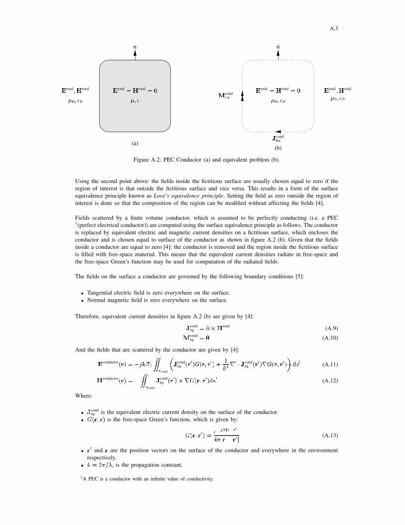
Figure A.2: PEC Conductor (a) and equivalent problem (b).

Using the second point above: the fields inside the fictitious surface are usually chosen equal to zero if the

region of interest is that outside the fictitious surface and vice versa. This results in a form of the surface

equivalence principle known as Love’s equivalence principle. Setting the field as zero outside the region of

interest is done so that the composition of the region can be modified without affecting the fields [4].

Fields scattered by a finite volume conductor, which is assumed to be perfectly conducting (i.e. a PEC1(perfect electrical conductor)) are computed using the surface equivalence principle as follows. The conductor

is replaced by equivalent electric and magnetic current densities on a fictitious surface, which encloses the

conductor and is chosen equal to surface of the conductor as shown in figure A.2 (b). Given that the fields

inside a conductor are equal to zero [4]: the conductor is removed and the region inside the fictitious surface

is filled with free-space material. This means that the equivalent current densities radiate in free-space and

the free-space Green’s function may be used for computation of the radiated fields.

The fields on the surface a conductor are governed by the following boundary conditions [5]:� Tangential electric field is zero everywhere on the surface.� Normal magnetic field is zero everywhere on the surface.

Therefore, equivalent current densities in figure A.2 (b) are given by [4]:Jcondeq = n�Htotal

(A.9)Mcondeq = 0 (A.10)

And the fields that are scattered by the conductor are given by [4]:Econductor(r) = �jkZ0�scond

�Jcondeq (r0)G(r; r0) + 1k2r0 � Jcond

eq (r0)rG(r; r0)�ds0 (A.11)Hconductor(r) = ��scond

Jcondeq (r0)�rG(r; r0)ds0 (A.12)

Where:� Jcondeq is the equivalent electric current density on the surface of the conductor.� G(r; r) is the free-space Green’s function, which is given by:G(r; r0) = e�jkjr�r0 j4�jr� r0j (A.13)� r0 and r are the position vectors on the surface of the conductor and everywhere in the environment

respectively.� k = 2�=�, is the propagation constant.

1A PEC is a conductor with an infinite value of conductivity.

A.4� Z0 =q�0�0 , is the characteristic impedance of the environment.� �0 is the permeability of the environment.� �0 is the permittivity of the environment.� ! = 2�f , where f is the frequency in Hz.

The derivation above may also be used for computing the fields that are scattered by a real conductor2 even

though a PEC was assumed during the derivation. This is because fields in a conductor are confined to a

thin layer on the surface at high frequencies, and the conductivity values of conductors are large enough for

the tangential field on the surface of the conductor to can be assumed negligible. Therefore, the boundary

conditions for a PEC are satisfied approximately in a real conductor.

A.2.2 Fields Scattered by the Substrate

Fields scattered by the substrate are computed using the volume and surface equivalence principles. The

details for computing the scattered fields using both principles are presented in the following sections.

A.2.2.1 Using the Volume Equivalence Principle

The substrate is removed and replaced by the equivalent volume electric and magnetic current densities,

which are defined by [6]: Jsubseq (r) = j!(�� �0)Etotal(r) (A.14)Msubseq (r) = j!(�� �0)Htotal(r) (A.15)

Where:� r is an arbitrary position vector in Vsubs, which is the region occupied by the antenna substrate.� � and � are the permittivity and permeability of the substrate material respectively.

Given that antenna substrates are non-magnetic material � = �0, and the volume equivalent magnetic current

density is zero.

The scattered fields are given by [6]:Esubstrate(r) = �jkZ�Vsubs

�Jsubseq (r0)G(r; r0) + 1k2r0 � Jsubs

eq (r0)rG(r; r0)�dv0 (A.16)Hsubstrate(r) = ��V Jsubseq (r0)�rG(r; r0)dv0 (A.17)

Where: r0 is arbitrary position vector in Vsubs, and r is an arbitrary position vector in the environment

including Vsubs.

A.2.2.2 Using the Surface Equivalence Principle

Using Love’s equivalence principle: fields that are scattered by the substrate and those inside the substrate are

computed using the equivalent problems that are shown in figure A.3 (b) and figure A.3 (c) respectively. The

dotted lines in figure A.3 represent the fictitious surface with equivalent current densities, and it is chosen

equal to the outer surface of the substrate. Using equations (A.7) and (A.8), and the continuity of tangential

fields: the equivalent current densities for both problems have equal magnitudes but are in opposite directions,

as indicated in figure A.3.

2A real conductor is used here to refer to a conductor with a finite conductivity value.

A.5

�; �Etotal;Htotal �0; �0Etotal;Htotal

n

�; �Etotal;Htotal �; �E;H = 0n�Msubseq �Jsubs

eq

�0; �0E;H = 0 �0; �0Etotal;Htotal

nMsubseq Jsubs

eq

(a)

(b) (c)

Figure A.3: Substrate (a) with outer (b) and inner (c) equivalent problems.

The equivalent current densities for the problem in figure A.3 (b) are given by:Jsubseq = n�Htotal

(A.18)Msubseq = �n�Etotal

(A.19)

And, the scattered fields are given by:Esubs(r) =� jkZ0"s�Jsubseq (r0)G(r; r0) + 1k2r0 � Jsubs

eq (r0)rG(r; r0)�ds0+"sMsubseq (r0)�rG(r; r0)ds0 (A.20)Hsubs(r) =� j kZ0 "s�Msubs

eq (r0)G(r; r0) + 1k2r0 �Msubseq (r0)rG(r; r0)�ds0�"s Jsubs

eq (r0)�rG(r; r0)ds0 (A.21)

Where: r0 is the position vector on the fictitious surface, r is the position vector everywhere in the

environment, and G(r; r0) is given by equation (A.13).

Fields inside the substrate are given by:Esubs(r) =jkZ"s�Jsubseq (r0)G(r; r0) + 1k2r0 � Jsubs

eq (r0)rG(r; r0)�ds0�"sMsubseq (r0)�rG(r; r0)ds0 (A.22)Hsubs(r) =j kZ "s�Msubs

eq (r0)G(r; r0) + 1k2r0 �Msubseq (r0)rG(r; r0)�ds0+"s Jsubs

eq (r0)�rG(r; r0)ds0 (A.23)

Where: r0 is the position vector on the fictitious surface, r is the position vector everywhere in the

environment, and G(r; r0) is given by equation (A.13) with k = !p��.

A.6

A.2.3 Integral Equations

It is concluded from the previous sections that:Etotal = Econd(Jcondeq ) +Esubs(Jsubs

eq ) +Esource(A.24)Htotal = Hconductor(Jcond

eq ) +Hsubs(Jsubseq ) +Esource

(A.25)

When using the volume equivalence principle for computation of the fields that are scattered by the substrate,

and: Etotal = Econd(Jcondeq ) +Esubs(Jsubs

eq ;Msubseq ) +Esource

(A.26)Htotal = Hcond(Jcondeq ) +Hsubs(Jsubs

eq ;Msubseq ) +Esource

(A.27)

When using the surface equivalence principle for computation of the fields that are scattered by the substrate.

Therefore, two equations are required for solution of Jcondeq and Jsubs

eq when using the volume equivalence

principle and three equations are required for solution of: Jcondeq , Jsubs

eq , and Msubseq ; when using the surface

equivalence principle. The required equations are derived by imposing field boundary conditions.

The first boundary condition, which is common when using the volume and surface equivalence principles is

the zero tangential electric field on the conducting surfaces of the antenna structure. This boundary condition

is imposed using the following equation:0 = n�Etotal(r) (A.28)0 = n�Econd(r) + n�Esubs(r) + n�Esource(r) (A.29)

Where: n is the outward pointing unit normal on the surface of the conductor, and r is the position vector on

the surface of the conductor. Econd is given by equation (A.11). Esubs depends on the equivalence principle

used for the computing the fields scattered by the substrate: it is given by (A.16) if the volume equivalence

principle is used, and equation (A.20) otherwise.

Equation (A.29) may be used on open conducting surfaces even though Econd is formulated for a closed

conducting surface [7]. An open conducting surfaces is an infinitesimally thin surfaces with defined boundaries

and is used for representing conducting plates of zero thickness. It is considered as the limiting case when

the thickness of the closed surface approaches zero, in which case the equivalent electric current density

(Jcondeq ) is the sum of the current on the top and bottom surfaces of the closed surface [7].

Derivation of the additional integral equations is presented in the following sections.

A.2.3.1 Using the Volume Equivalence Principle

The additional equation that is required is derived using the definition of the volume equivalent electric

current density (equation (A.14)).

The definition of the equivalent electric current density is re-written in terms of the total electric as follows:Etotal(r) = j!(�0 � �)Jsubseq (r) r 2 Vsub (A.30)

Substituting Etotal from equation (A.5) into the above equation gives:Econductor(r) +Esubstrate(r) +Esource(r) = j!(�0 � �)Jeq(r) r 2 Vsub (A.31)Econd and Esubs are given by equations (A.11) and (A.16) respectively.

A.7

A.2.3.2 Using the Surface Equivalence Principle

The two additional equations that are required for solution of the current densities are derived by imposing

the boundary conditions on the fictitious surface for both the problems in figure A.3 (b) and (c). This is

achieved using either the definition of the equivalent electric or magnetic current densities in either case.

However, the equations that results from using the definitions of the equivalent electric and magnetic current

densities for both the inner and outer equivalent problems, do not give unique solutions at the frequencies

that are equal to the resonant frequencies of the cavity formed by the fictitious surface [6]. This problem

is averted by using the CFIE (Combined Field Integral Equations), which is the weighted sum of the EFIE

(Electric Field Integral Equation) and MFIE (Magnetic Field Integral Equation) given by [6]:�EFIE + Z(1� �)n� MFIE

Where:� � is a dimensionless number between zero and one.� Z0 is the intrinsic impedance.� EFIE and MFIE are the equations, which results from using the definitions of the equivalent magnetic

and electric current densities respectively.� is chosen as 0.5 for this application in-line with the argument in [6, p. 465] that choosing � as such,

results in the optimum combination of the EIFE and MFIE.

The EFIE and MFIE for the problem in figure A.3 (b) are derived using equations (A.18) and (A.19)

respectively, and are given by:�Msubseq (r) = n�Econd(r) + n�Esubs(r) + n�Esource(r) (A.32)Jsubseq (r) = n�Hcond(r) + n�Hsubs(r) + n�Hsource(r) (A.33)

Where r and n are the position vector and unit normal on the surface of the substrate. The required CFIE

is given by: n�Esource(r)� Zn� n�Hsource(r) =Zn� n�Hcond(r)� n�Econd(r)+Zn� n�Hsubs(r)� n�Esubs(r)�Msubseq (r)� Zn� Jsubs

eq (r) r 2 Ssub

(A.34)

Where: Econd(r) and Hcond(r) given by equations (A.11) and (A.12) respectively, and Esubs(r) and Hsubs(r)given by equations (A.20) and (A.21) respectively.

The CFIE for the problem in figure A.3 (c) is derived following a similar procedure, but the equivalent current

densities of the inner equivalent problem are equal to those of the problem in figure A.3 (b) multiplied by

minus one. The problem in figure A.3 (c) only involves equivalent current densities radiating in an infinite

homogeneous medium, therefore: Etotal = Esubstrate(A.35)Htotal = Hsubstrate(A.36)Esubs and Hsubs are given by equations (A.22) and (A.23) respectively. The resulting CFIE is given by:n�Esubstrate(r) + Zn� n�Hsubstrate(r) =Msubs

eq + Zn� Jsubseq r 2 Ssub (A.37)

A.2.4 Discussion

The MoM formulations are given by:

1) Equations (A.29) and (A.31). These equations may be used for computing Jcondeq and Jsubs

eq , which may

then be used for computing the neccessary antenna parameters.

A.8

2) Equations (A.29), (A.34), and (A.37). These equations may be used for computing Jcondeq , Jsubs

eq andMsubseq , which may then be used for computing the neccessary antenna parameters.

Both formulations may be used with printed antennas of arbitrary configuration. However, only the

formulation using the volume equivalence principle may be used for the analysis of antennas with

inhomogeneous substrates, where: the different regions of the substrate with different electromagnetic

properties are represented by different volume equivalent electric current densities, which are defined by

equation (A.14); substituting values of � as necessary.

A.3 FEM-MoM Formulation

One of the strong points FEM is the straight forward treatment of complex geometries and material

inhomogeneities [8, p. 15]. The probe-fed printed antenna structure is a complex structure, given that it

is composed of an arbitrary configuration of: conducting strips, conducting wires, and, a dielectric (which

can be inhomogeneous). Therefore, FEM is better suited for the analysis of these structures.

FEM analysis of these structures involves computing the electric field in the region that the structure occupies,

imposing the necessary boundary conditions on the conducting regions and feed area. The electric field is

computed using the electric field wave equation, which is given by:r�� 1�r�E�� !2�E = �j!J+r� M� (A.38)

Where J and M are the impressed electric and magnetic current densities within the substrate of the antenna

structure.

The solution of equation (A.38) for the electric field using FEM, can be computed only over a finite volume

region (V ) and not all space. This is because the FEM solution involves reducing the equation that governs

the problem into a matrix equation, and the size of the matrix in the equation is proportional to the volume

region. Therefore, V is defined here as the region occupied by the antenna and is enclosed by a fictitious

surface (S), which does not touch the conducting surfaces of the antenna structure.

Solution of equation (A.38) within V requires specification of the fields on S to make it seem as if the

volume region is infinite and not truncated [2]. Since the interest is only on the electric field inside S, the

problem is reduced to a problem that is equivalent to the original problem inside S. This is done using

Love’s equivalence principle, and the equivalent problem is shown in A.4 (b) with Meq and Jeq given by:Jeq = n�H (A.39)Meq = �n�E (A.40)

Either Meq or Jeq may be used as the required boundary condition on S, but since the electric field is being

computed it is easier to use Jeq as a boundary condition since its directly related to the tangential magnetic

field on S.

However, Meq and Jeq are not known. Since Meq is related to E: there are only two unknowns, i.e. E orJeq. The formulation for the FEM analysis gives the relation between E and Jeq. Therefore, another equation

is required for solution of E and Jeq.

The additional equation is derived using a problem derived using Love’s equivalence principle, which is

equivalent to the antenna problem outside S. This problem is shown in figure A.4 (c), and it involves

equivalent current densities on S radiating in free-space. The analysis of this problem for Meq and Jeq is

performed using MoM as it resembles the problems of section A.2.

A.9

Substrate

ScondJM �; � �0; �0E;H(a)

E;H = 0�0; �0 E;H�0; �0n

Meq Jeq

(c)

SJM �; ��0; �0 �0; �0E;H = 0E;H Vn�Meq

-Jeq

(b)

Figure A.4: Arbitrary printed antenna structure (a) with inner (b) and outer (c) equivalent problems.

A.3.1 FEM Formulation

FEM formulation is the equation that is solved using FEM for the electric field. There are two methods that

are used for deriving the FEM formulation, namely: the Rayleigh-Ritz and Garlerkin methods. These methods

are discussed in detail in [6], [2], [5]. The formulation in this section is derived using the Rayleigh-Ritz

method, where the formulation is a functional or variational principle. This is a function, which is formulated

in terms of the electric field and is made stationary by the electric field that satisfies equation (A.38) under

given boundary conditions [6], [8].

The generalised variational principle that is presented in [6, Chapter 6] is used as the FEM formulation. It

is given by: F (E) =12�V � 1�r (r�E) � (r�E)� k20�rE �E�dV+�S � e2 (n�E) � (n�E) +E �U�dS+�V �jk0Z0E � J+E � (r� M� )� dV (A.41)

Where e and U are parameters that are related to the boundary conditions. The unknown Jeq is incorporated

into the formulation as follows. The first variation of the equation (A.41) gives the integrand of the surface

integral, which equals to zero for: 1�r n� (r�E) + en� (n�E) = U (A.42)

Maxwell’s electric field curl equation is given by:r�E(r) = �j!�H(r) (A.43)

The dot product of the unit normal on S with equation (A.43) results in:n� (r�E(r)) = �j!�n�H(r) (A.44)

A.10

The above equation is equal to equation (A.42), for: e = 0 (A.45)U = �j!�0H(r) (A.46)

Therefore, setting e and U as above in equation (A.41) results in:F (E) =12�V � 1�r (r�E) � (r�E)� k20�rE �E� dV+�V �jk0Z0E � J+E � (r� M� )�dV�jk0Z0"S E � (n�H)dS (A.47)

Which can be written in another form using equation (A.39) and figure A.4, as:F (E) =12�V � 1�r (r�E) � (r�E)� k20�rE �E� dV+�V �jk0Z0E � J+E � (r� M� )�dV+jk0Z0"S E � JeqdS (A.48)

A.3.2 MoM Formulation

Following section A.2.3.2; a CFIE is also used here as the MoM formulation. The required CFIE is derived

using the definitions of the equivalent electric and magnetic current densities, and is given by:Meq(r)� Z0n� Jeq(r) = �n�E(r)� n� n�H(r) r 2 S (A.49)E and H are the fields that are radiated by the equivalent currents, and they are given by:E(r) =� jkZ"s�Jeq(r0)G(r; r0) + 1k2r0 � Jeq(r0)rG(r; r0)�ds0+"sMeq(r0)�rG(r; r0)ds0 r0 2 S (A.50)

And: H(r) =� j kZ "s�Meq(r0)G(r; r0) + 1k2r0 �Meq(r0)rG(r; r0)�ds0�"s Jeq(r0)�rG(r; r0)ds0 r0 2 S (A.51)

A.3.3 Discussion

Equations (A.48) and (A.49) may be used for solution of: Jeq and Meq on S, and E within V . Jeq andMeq may then be used for computing the fields radiated by the antenna everywhere, except inside V .

A.4 Feed Model

The antenna is fed by an ideal voltage source applied between the inner and outer conductors of the probe

feed at the feed opening (see figures A.1 and A.5). This source voltage creates electric and magnetic fields

inside the feed opening and the field mode can be assumed to be TEM for most practical purposes [9](see

figure A.5 (b)).

Numerous approaches have been proposed for modeling this type of feed in the literature [2], [4], [6].

The common approach is to specify the fields in the feed opening. Two popular methods that are used for

A.11

ri

ro(0,0,0)

rpc

H(b)(a)

Coaxial Aperture

Inner Conductor

Outer ConductorEFigure A.5: Cross-section of a probe-fed printed antenna without substrate (a) and the feed opening (b).

specifying the fields across the coaxial aperture are [4, p. 722-726]: the magnetic frill generator, and the

delta-gap model. The other less common approach is to specify the current distribution on the inner conductor

(see figure A.5) of the feed. This approach has been used successfuly with FEM formulation [10], therefore,

it is discussed for use with the FEM formulation only.

A.4.1 Magnetic Frill Generator

A ring of infinitesimaly thin, circumferentially directed equivalent magnetic current density is placed across

the feed opening with this model. This equivalent magnetic current density is defined as [11]:Msourceeq = �2n�Eaperture

(A.52)

Where: Eaperture is the electric field across the feed opening, and n is the normal at the feed opening, which

points away from the coaxial cable. Given that TEM mode fields are assumed in the feed opening, Eaperture

is given by [4]: Eaperture(r) = 8<: Vapp2jr� rpcjln(ro=ri) r 2 saperture0 otherwise

(A.53)

Where: Vapp is the voltage across the inner and outer conductors of the coaxial feed at the point where the

coaxial cable attaches to the antenna structure, Saperture is the feed opening region, and the definitions of rpc,

ro, and ri can be seen in figure A.5.

The magnetic current density in equation (A.52) is defined using the surface equivalence principle in

conjunction with image theory [11], assuming that the aperture exists on an infinite PEC ground plane.

Therefore, this source model is appropriate for cases where the feed opening exist on a conducting strip that

is large enough for the formulation to be valid, and is not near the edges of the conducting strip.

A.4.1.1 Use with the MoM Formulation

This feed is incorporated into the MoM formulation by, using fields radiated by the magnetic frill current asEsource and Hsource, i.e. [4]:Esource(r) = �sMsourceeq (r0)�rG(r; r0)ds0 (A.54)Hsource(r) = �j kZ "s�Msource

eq (r0)G(r; r0) + 1k2r0 �Msourceeq (r0)rG(r; r0)�ds0 (A.55)

Where G(r; r0) is the free-space Green’s function. The feed opening and inner conductor are treated as part

of the conducting strips, and the zero tangential electric field boundary condition is applied on their surfaces.

A.12

A.4.1.2 Use with the FEM Formulation

This feed model is incorporated into the FEM formulation by substituting the magnetic current density of

equation (A.52) in the FEM formulation (equation (A.48)), and the inner conductor of the feed is treated as

part of Scond and the tangential electric field component is set to zero on its surface.

A.4.2 Delta Gap Model

With the delta gap model: the electric field across the coaxial aperture is assumed to be constant such that:Eaperture(r) = Vapp(ro � ri) r (A.56)

And: Haperture(r) = jEaperturejZ � (A.57)

This model is accurate for cases where ro � ri is small compared to the wavelength (at the frequency of

simulation) for a constant field distribution to be assumed across the feed opening.

A.4.2.1 Use with the MoM Formulation

This source model is also incorporated into the MoM formulations via the Esource and Hsource terms. Using

the above equations, the source electric and magnetic fields are given as:Esource(r) = (Eaperture(r) r 2 saperture0 otherwise(A.58)

And: Hsource(r) = 8<: jEaperturejZ � r 2 saperture0 otherwise

(A.59)

The feed opening and inner conductor are treated as part of the conducting strips, and the zero tangential

electric field boundary condition is applied on their surfaces.

A.4.2.2 Use with the FEM Formulation

The feed voltage is incorporated into the FEM formulation as a Dirichlet boundary condition and is imposed

the same way the zero tangential field boundary condition on Scond is imposed. The inner conductor is treated

as a part of Scond.

A.4.3 Probe Feed Model

The inner conductor (see figure A.5 (a)) is replaced by an infinitesimally thin current filament of the same

length. A constant electric current density (J) is assumed throughout the length of the current filament. The

feed opening is treated as part of the conducting strip that the coaxial cable attaches to.

Assuming a z directed inner conductor; the electric current density in equation (A.47) is given by [2]:J(r) = IÆ(x� xs)Æ(y � ys)z (A.60)

Where: I is the magnitude of the current on the probe-feed, and xs and ys are the x and y components of

the center of the inner conductor. This feed model is incorporated into the FEM formulation by substituting

A.13

the electric current density of equation (A.60) into equation (A.47). The feed opening is treated as part of

the conducting strips of the antenna structure.

This source model gives accurate results for antennas with thin dielectric substrates and for instances where

the diameter of the inner conductor can be ignored [6]. When the diameter of the inner conductor cannot be

ignored the strip model [12] may be used; where the inner conductor is represented by two current filaments

placed as shown in figure A.6. w in figure A.6 is given by:w = 4ric (A.61)

Where ric is the radius of the inner conductor of the coaxial cable.

Axis through center of inner conductor

w/2 w/2

Figure A.6: Positions of the current filaments (solid black lines) using the strip model.

A.5 Choice of Formulation

The formulations presented in this paper have been used successfully for analysis of printed antennas in

[13], [14], [15], [16], [17]. All the formulations are expected to be equally accurate given that no simplifying

assumptions are made during their derivations, except with feed models, which are used with all the

formulations. Therefore, criterion for the formulation to be implemented in SuperNEC is based on the

efficiency of its numerical solution in terms of:� Memory usage� Solution Time

The formulations presented in the preceding sections are solved for the unknown quantities (i.e. current

densities and/or electric field) using FEM and/or MoM. The approach that is adopted with both numerical

techniques is to reduce the formulation into a matrix equation, which can be solved using a computer. This

is done by expanding the unknown quantities by a sum of weighted basis functions, and the weights become

the new unknowns. The weights are determined by reducing each of the formulation equations into a matrix

equation involving the sum of a square matrix-column vector product, for each of the unknown quantities in

the equation. The resulting matrix equations for each of the formulation equations are then solved together

for the unknown weights.

The memory usage criterion above is important because the matrices that are generated during the solution

process can be large for problems involving printed antennas. These matrices have to be stored and the

solution of the matrix equations also requires memory. The time required to fill and solve the resulting

matrices is also important because the antenna structure can only be analysed for the parameter of interest

(e.g. input impedance) per frequency using the formulations presented in this appendix and the variation of

the impedance might be required for a large frequency band.

A.14

The memory requirement and solution time for the numerical solution of the formulations presented in the

preceding sections, are compared and the formulation, which requires the least memory and time for solution

of the unknown quantities is chosen for implementation in SuperNEC.

A.5.1 Memory Usage

The memory that is required for a numerical solution using FEM and MoM is for storage of the matrices

that are generated during the solution process and solution of the resulting matrix equations.

A.5.1.1 Storage of Matrices

The amount of memory required for storage of a matrix that results for a problem with n-unknowns is:� Less than �nM when using FEM [6, p. 586]. Where: � is the largest number of elements that an

unknown variable is associated with, and M is the amount of memory required to store a matrix entry.

This is because FEM formulations result in sparse matrices with a large number of matrix entries equal

to zero, and only the non-zero entries are stored.� Equal to n2M when using MoM. This is because MoM formulations result in full matrices.

Therefore, MoM implementations require more memory when compared to FEM implementations for a

problem with an equal number of unknowns.

Printed antenna problems analysed using FEM generally result in more unknowns than equivalent problem

analysed using MoM. This is because the FEM analysis includes the region surrounding the structure while

only the structure is considered with MoM. Matrices resulting from a FEM analysis do not necessarily

require more memory for storage when compared to the matrices that result from a MoM analysis of the

same problem. To give an example: a problem that is analysed using FEM with 60000 unknowns requires

the amount of memory, which is less than that required by an equivalent problem analysed using MoM

with 949 unknowns; assuming that � = 15. It unlikely that an equivalent MoM problem analysed using

the formulations presented in this appendix will have the number of unknowns less than 949, based on

experience.

Table A.1: Matrices generated for the different formulations.

Formulation Matrix Quantity Size Sparse/Full

MoM Formulation (Volume Equivalence Principle) Jcondeq 2 Nc� Nc FullJsubseq 2 NV

s � NVs Full

MoM Formulation (Surface Equivalence Principle) Jcondeq 3 Nc� Nc FullJsubseq 3 NS

s� Nc FullMsubseq 3 NS

s� NSs Full

FEM-MoM Formulation Jeq (MoM) 1 Nb� Nb FullJeq (FEM) 1 Nb� Nb SparseMeq (MoM) 1 Nb� Nb FullE (FEM) 1 Ne� Ne Sparse

Table A.1 gives a breakdown of the matrices that are generated for the numerical solution of the different

formulations. The variables for the sizes of the matrices are defined as follows:� Nc is the number of unknowns that are associated with the electric current density on the conducting

surface of the structure.� NSs is the number of unknowns that are associated with the equivalent electric and magnetic current

densities on the surface of the substrate.

A.15� Nd is the number of unknowns that are associated with the equivalent electric and magnetic current

densities on the enclosing surface of the FEM problem domain.� NVs is the number of unknowns that are associated with the equivalent volume electric current density.� Ne is the number of unknowns that are associated with the electric field within the FEM problem domain.

The variables above, are presented in order of increasing value and their values are proportional to the size of

the antenna and the frequency at which the analysis is performed. The exact values of the variables depend

on a particular problem, but the following relation holds in general:� Nc is always smaller than all the variables,� The values of NSs and Nd are comparable.� NV

s is considerably larger than NSs and Nd.� Ne is the largest and its value is greater than the sum of all the other variables combined. Its value

depends on the structure that is being simulated, but it will most likely not be more than 50*NVs .

Based on table A.1 and the above paragraph: the amount of memory required for storage of the matrices

resulting from the FEM-MoM formulation is expected to be less than that required for storage of the resulting

matrices from the numerical solutions of the other formulations for an equivalent problem. This is because:� The numerical solution of the MoM formulation results in 6 matrices, which are comparable to two

of the matrices of the FEM-MoM formulation resulting from the MoM formulation part, in size. With

regard to the matrices resulting from the FEM formulation part; there are 7 more full matrices compared

to two sparse matrices resulting from the FEM formulation: one of the matrices is the same size as

the matrices resulting from the MoM formulations, but requires less memory for storage, and the other

is appreciably larger than all the matrices, but since its sparse the memory required is less than that

required for storage of most of the matrices.� The memory required by the MoM formulation using the volume equivalence principle is expected to

be greater than that required by the FEM-MoM formulation. The two matrices, which result from the

MoM formulation part are smaller than those from the MoM formulation using the volume equivalence

principle, for the volume equivalent current term. This is because matrices from the MoM formulation

part of the FEM-MoM formulation result from the discretisation of the surface, which encloses the FEM

problem domain and those from the MoM formulation using surface equivalence principle results from

the volume discretisation of the substrate. Even though the size of Ne is larger than that of NVs ; the

amount of memory required to store the matrix for the electric field will be equal or comparable to that

for storing the matrix for the volume equivalent current density term for Ne appreciably larger than NVs .

The number of unknowns depends on the problem being solved, and it cannot be readily shown that the FEM-

MoM formulation will require less memory. However, if one considers that the amount of memory that is

required to store a matrix resulting from a FEM formulation increases linearly with the number of unknowns

and that resulting from the MoM formulation increases quadratically with the number of unknowns, then it

can be appreciated that the FEM-MoM formulation is likely the more memory efficient formulation, since

antenna simulation problem generally result in a large number of unknowns.

A.5.1.2 Solution of Matrix Equations

The memory required for solution of the resulting matrix depends on the method used for solving the resulting

matrices.

When using direct solvers, the required memory depends on the size of the matrix being solved. The resulting

matrix equation for the FEM-MoM formulation will require more memory for solution using a direct solver

because of the large number of unknowns associated with a FEM analysis.

When using an iterative solver the amount of memory required for solution of the matrix equation depends

on: the size of the matrix (but is considerably less than that required by a direct solver), and the properties

of the matrices. The memory required by iterative solvers is for computation of the matrix-vector product.

Matrices resulting from the FEM-MoM formulation are sparse, and matrix multiplication with a sparse matrix

A.16

is memory efficient. It is shown in [6, p. 470-480] that the matrices resulting from the FEM-MoM formulation

can be solved with relatively less memory using iterative solvers.

Therefore, it is not clear which formulation will require more memory for solution of the resulting matrix

equations since it depends on the method used for solving the resulting matrix equations.

A.5.2 Solution Time

Solution time for both numerical methods is determined by the time required to fill the required matrices

and time required to solve the matrix equations.

A.5.2.1 Matrix Fill Time

The time required to generate a matrix entry for the FEM formulation is appreciably less than that required

to generate an entry for the MoM formulation. This is so because:� The terms for the MoM matrices involves evaluation of two integrals, compared to a single integral

with FEM: the two integrals are the testing integral (see appendix C) and integral in the formulation

equations.� The integral terms of the MoM formulation are more complicated than those of the FEM formulations.� The singularities in the integrands of the MoM formulation, require introduction of additional terms for

evaluation [6]. This increase the time it takes to compute a matrix entry.� Each unknown in a MoM system is coupled with all the other unknowns, resulting in full matrices,

and with FEM the unknowns are only related to a few of the elements (15 at most as indicated above).

Therefore, fewer terms are evaluated for FEM formulations as compared to MoM formulations.

The time required to fill the matrices for the FEM-MoM formulation is expect to be less than that required

to fill the matrices for the other formulations. This is because:� 4 fully populated matrices have to be filled with the MoM formulation using the volume equivalence

principle.� 9 fully populated matrices have to be filled with the MoM formulation using the surface equivalence

principle.� 2 fully populated and 2 sparse matrices are filled using the FEM-MoM hybrid formulation.

A.5.2.2 Matrix Solution Time

The time required to solve the resulting matrices depends on the matrix solver that is used. The solution

time is proportional to the size of the matrix when using a direct solver. The solution time is proportional

to the time it take to compute a the matrix-vector product and the number of iterations before convergence.

The matrix-vector product depends on the number of elements contained in the matrix, i.e. whether is full

or sparse, as the matrix-vector product can be computed efficiently using for a sparse matrix. The number of

iterations depends on the condition number of the matrix, which may be improved by using a pre-conditioner

[6].

Therefore, more time will be required for solution of the matrices resulting from the FEM-MoM formulation

since the size of the matrix resulting from the FEM formulation is large. However, the the matrices resulting

from the FEM-MoM formulation may be solved in less time using a pre-conditioner that is developed in

[18], which may also be computed efficiently.

Therefore, it is not clear which formulation will require more time for solution of the resulting matrix

equations since it depends on the method used for solving the resulting matrix equations.

A.17

A.5.3 Discussion

The FEM-MoM formulation is chosen for implementation in SuperNEC because it is likely to be more

memory efficent when compared to the other formulations given that the matrices resulting from the FEM

formulation part are sparse and the amount of memory required for storage increases linearly with the number

of unknowns, and the time required to fill the matrices resulting from the formulation is less than that for

the other formulations. The memory and time required for solution of the resulting matrices depend on the

matrix solver that is used and are therefore not used as a selection criterion.

A.6 Conclusion

The derivation of two MoM formulations and a FEM-MoM formulation for analysis of probe-fed printed

antennas have been presented together with different models for representing the antenna feed. The

formulations are then compared on the basis of memory usage and time required for solution of the unknown

parameters.

The FEM-MoM formulation is selected for implementation in SuperNEC. It is argued that its numerical

solution using FEM and MoM will be more memory efficient and that is will require less time to fill the

matrices generated for the formulation when compared to the two MoM formulations. The memory and time

required for solution of the resulting matrix equations is not used as a criterion because it depends on the

matrix solver that is used.

References

[1] G. Burke and A. Pogio. “Numerical Electromagnetics Code (NEC) - Method of Moments. Part 1: Program

Description-Theory.” Tech. Rep. Report UCID 18834, Lawrence Livermore National Laboratory, 01 1981.

[2] L. K. J.L. Volakis, A. Chatterjee. Finite Element Method for Electromagnetics: Antennas, Microwave Circuits, and

Scattering Applications. New York: IEEE Press, first ed., 2001.

[3] K. Chen. “A Mathematical Formulation of the Equivalent Principle.” IEEE Transactions on Microwave Theory and

Techniques, vol. 37, no. 10, pp. 1576–1581, 10 1989.

[4] C. A. Balanis. Advanced Engineering Electromagnetics. John Wiley and Sons, first ed., 1989.

[5] P. P. Silvester and G. Pelosi. Finite Element for Wave Electromagnetics. IEEE Press, first ed., 1994.

[6] J. Jin. The Finite Element Method in Electromagnetics. New York: John Wiley and Sons, Inc., second ed., 2002.

[7] E. Newman and D. Pozar. “General Integral Equation Formulation for Microstrip Antennas and Scatters.” IEE

Proceedings, vol. 132, no. 12, pp. 424–432, 7 1985.

[8] D. B. Davidson. Computational Electromagnetics for RF and Microwave Engineering. Cambridge, first ed., 2005.

[9] J. Gong and J. L. Volakis. “An Efficient and Accurate Model of a Coax Cable Feeding Structures for FEM

Simulations.” IEEE Transactions on Antennas and Propagation, vol. 43, no. 12, pp. 1474–1478, 12 1995.

[10] J.-M. Jin and J. L. Volakis. “A Hybrid Finite Element Method for Scattering and Radiation by Microstrip Patch

Antennas and Arrays Residing in a Cavity.” IEEE Transactions on Antennas and Propagation, vol. 39, no. 11, pp.

1598–1604, 11 1991.

[11] L. L. Tsai. “A Numerical Solution for the Near and Far Fields of an Annular Ring of Magnetic Current.” IEEE

Transactions on Antennas and Propagation, vol. 20, no. 05, pp. 569–576, 09 1972.

[12] H. Wang, Y. Jin, and T. H. Hubing. “Finite-Element of Coaxial Cable Feeds and Vias in Power-Bus Structure.” IEEE

Transactions on Electromagnetic Compatibility, vol. 40, no. 04, pp. 569–574, 11 2002.

[13] P. Katehi and N. Alexopoulos. “On the Effect of Substrate Thickness and Permittivity on Printed Circuit Dipole

Properties.” IEEE Transactions on Antennas and Propagation, vol. 31, pp. 34 – 39, 01 1983.

[14] B. Salman and A. McCowen. “The CFIE Technique Applied to Finite-Size Planar and Non-Planar Microstrip

Antenna.” pp. 338–341. IEE, 04 1996.

[15] T. K. Sarkar, S. M. Rao, and A. R. Djordjevi� . “Electromagnetic Scattering and Radiation from Finite Microstrip

Structures.” IEEE Transactions on Microwave Theory and Techniques, vol. 38, no. 11, pp. 1568–1575, 11 1990.

A.18

[16] M. W. Ali, T. H. Hubing, and J. L. Drewniak. “A Hybrid FEM/MOM Technique for Electromagnetic Scattering

and Radiation from Dielectric Objects with Attached Wires.” IEEE Transactions on Electromagnetic Compatibility,

vol. 39, no. 04, pp. 304–314, 11 1997.

[17] S. Makarov, S. Kulkarni, A. Marut, and L. Kempel. “Method of Moments Solution for a Printed Patch/Slot Antenna

on Thin Finite Dielectric Substrate Using the Volum Integral Equation.” IEEE Transactions on Antennas and

Propagation, vol. 54, no. 04, pp. 1174–1184, 04 2006.

[18] J. Lui and J.-M. Jin. “A Highly Effective Preconditioner for Solving the Finite Element-Boundary Integral Matrix

Equation of 3-D Scattering.” IEEE Transactions on Antennas and Propagation, vol. 50, no. 9, pp. 1212–1221, 9

2002.

B.1

Appendix B

Numerical Results

B.1 Introduction

The FEM (Finite Element MEthod)-MoM (Method of Moments) formulation presented in section A.3 of

appendix A is implemented in a software application using the probe feed model. The software application is

developed as a stand alone executable, which will be integrated into SuperNEC. The software was developed

using C++ with certain modules created using Matlab. It can be used for analysis of probe-fed printed

antennas using the probe-feed model (see section A.4.3 of appendix A). Details of the software application

may be obtained in appendix F.

Structures that are analysed using the software application are represented as a connection of tetrahedrons for

three dimensional objects and a connection triangles for are two dimensional objects. These connections of

triangles and tetrahedrons are called meshes, and are discussed in more detail in appendix F. The size of the

triangles or tetrahedrons in the mesh depends on the frequency at which the structure is being analysed. The

rule of thumb for the sizes of the triangles or tetrahedrons is that [1, p. 5]: the triangles must be constructed

such that there are 100 segments per square wavelengths, and the tetrahedrons must be constructed such

that there are 1000 segments per cubic wavelength. The segments in the preceding statements are the line

segments, which connects the different corners of the triangle or tetrahedron. The above are just guidelines

and better results are obtained using more segments per square or cubic wavelength.

Numerical results computed using the software application for the radar cross section of a PEC (perfect

electrical conductor) sphere and the input impedance of a probe-fed printed antenna are presented to illustrate

correct implementation of the formulation. The presentation is structured as follows. The results for the radar

cross section of a sphere are presented in section B.2, and those for the input impedance of a probe-fed

printed antenna are presented in section B.3.

B.2 Radar Cross Section of PEC Sphere

Computed results for the monostatic and bistatic radar cross sections of a PEC sphere are presented. Results

for the monostatic rcs (radar cross section) are computed using the MoM formulation part of the FEM-

MoM formulation, and those for the bistatic rcs are computed using the FEM-MoM formulation. The results

computed using the MoM formulation are compared to the Mie-series solution, and those computed using the

FEM-MoM formulation are compared to those computed using the MoM formulation for a similar problem.

The MoM formulation part of the formulation is used for analysis of a PEC sphere by setting the Meq

contribution to zero, which according to section A.2.1 of appendix A, is equivalent to setting the tangential

component of the electric field equal to zero.

B.2

B.2.1 Monostatic Radar Cross Section

The configuration for this example is shown in figure B.1, where a PEC sphere of radius 0.1 m is excited

by a -z-directed plane wave with a y directed linearly polarised electric field vector. The rcs is computed for

the following frequency range: 100 MHz to 3050 MHz.

x z y

EH r

Figure B.1: PEC sphere illuminated by plane wave.

The computed rcs is shown together with the Mie-series solution in figure B.2. It can be seen in the figure that

the computed rcs compares well with the Mie-series solution. The difference at higher frequencies starting at

around 2 GHz is due to interpolation errors. The mesh used for representing the structure is not fine enough

for the frequencies above 2 GHz. This may be improved by using finer mesh, i.e. increasing the number of

segments per square wavelength.

B.2.2 Bistatic Radar Cross Section

A sphere covered by a dielectric coat is used with the FEM-MoM formulation, where the electromagnetic

properties of the dielectric coat are similar to those of free-space. The thickness of the coat is selected such

that only a single layer of tetrahedrons represents the coat in the mesh. The MoM solution was computed

using a the same problem configuration as in section B.2.1 with a different radius sphere.

The problem configuration of the coated sphere is shown in figure B.3. The excitation plane wave is a -z

directed plane wave with a y directed linearly polarised plane wave. The rcs is computed at � = 00 and00 � � � 1800 .

The computed results are shown in figure B.4. It can be seen that there is excellent agreement between results

obtained using the MoM and FEM-MoM formulations.

B.3 Printed Antenna Impedance

In this section the results for computation of the input impedance of a probe-fed patch antenna in figure B.5

are presented. The input impedance is computed for the following frequency range: 600 MHz to 1300 MHz.

B.3

0 0.5 1 1.5 2 2.5 3 3.50

0.02

0.04

0.06

0.08

0.1

0.12

Frequency (GHz)

Monosta

tic R

CS

(m

2)

Mei−Series

Computed

Figure B.2: Monostatic RCS of a PEC sphere.

R1

R2Dielectric Coat

R1 = 436.7 mm

R2 = 336.7 mmx z y

HE r

Figure B.3: Coated PEC sphere illuminated by a plane wave.

The computed input reactance and magnitude of the input impedance are shown compared with the results

from [2]. Results from [2] are computed using a hybrid FEM-MoM formulation where the FEM formulation

is used for the analysis of the substrate and MoM for conducting outside the substrate [3]. Their results

compare successfully with measurement, and they were computed using a similar feed model.

The phase shift at around 1250 MHz is due to discretisation errors. A coarse mesh is used to limit the

number of unknown because a direct solver is used for solution of the resulting matrices. The results may be

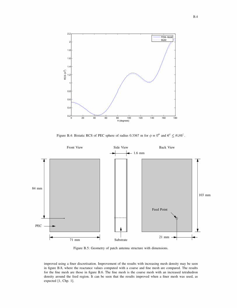
B.4

0 20 40 60 80 100 120 140 160 1800.2

0.4

0.6

0.8

1

1.2

1.4

1.6

1.8

2

2.2

θ (degrees)

RC

S (

m2)

FEM−MoM

MoM

Figure B.4: Bistatic RCS of PEC sphere of radius 0.3367 m for � = 00 and 00 � �1800 .

1.6 mm

71 mm

103 mm

84 mm

21 mm

Back ViewSide ViewFront View

Substrate

PEC

Feed Point

Figure B.5: Geometry of patch antenna structure with dimensions.

improved using a finer discretisation. Improvement of the results with increasing mesh density may be seen

in figure B.8, where the reactance values computed with a coarse and fine mesh are compared. The results

for the fine mesh are those in figure B.6. The fine mesh is the coarse mesh with an increased tetrahedron

density around the feed region. It can be seen that the results improved when a finer mesh was used, as

expected [1, Chp. 1].

B.5

600 700 800 900 1000 1100 1200 1300 1400−40

−30

−20

−10

0

10

20

30

40

50

Frequency (MHz)

Reacta

nce (

Ohm

s)

Computed

Ji, Hubing, and Drewniak

Figure B.6: Reactance of the patch antenna as a function of frequency.

600 700 800 900 1000 1100 1200 1300 14000

10

20

30

40

50

60

70

80

90

Frequency (MHz)

Impedance M

agnitude (

Ohm

s)

Computed

Ji, Hubing, and Drewniak

Figure B.7: Impedance magnitude as a function of frequency.

B.6

600 700 800 900 1000 1100 1200 1300 1400−40

−30

−20

−10

0

10

20

30

40

50

Frequency (MHz)

Reacta

nce (

Ohm

s)

Fine Mesh

Coarse Mesh

Figure B.8: Results for a coarse and fine mesh of the antenna structure.

B.4 Conclusion

Numerical results computed using the software application for the radar cross section of a PEC (perfect

electrical conductor) sphere and the input impedance of a probe-fed printed antenna are presented. Results

for the monostatic and bistatic rcs of a sphere, computed using the MoM and FEM-MoM formulations

respectively are shown and compared to the Mie-series solution and MoM formulation respectively. Results

for the input impedance are shown compared to result from a previous publication.

Excellent agreement is obtained for all the radar cross sections results. The input impedance results compared

well with the results from a previous publication but there was a notable phase shift at high frequencies,

which is believed to be due to interpolation errors and could be improved using a mesh with more segments

per cubic wavelengths.

References

[1] D. B. Davidson. Computational Electromagnetics for RF and Microwave Engineering. Cambridge, first ed., 2005.

[2] Y. Ji, T. Hubing, and J. Drewniak. “Finite Element Modelling of Patch Antenna and Cavity Sources.” In IEEE

International Symposium on Electromagnetic Compatibility, 2000, vol. 2, pp. 811–814. 08 2000. ISBN: 0-7803-5677-

2.

[3] M. W. Ali, T. H. Hubing, and J. L. Drewniak. “A Hybrid FEM/MOM Technique for Electromagnetic Scattering

and Radiation from Dielectric Objects with Attached Wires.” IEEE Transactions on Electromagnetic Compatibility,

vol. 39, no. 04, pp. 304–314, 11 1997.

C.1

Appendix C

Reduction of MoM Formulation into a Matrix

Equation

C.1 Introduction

MoM (Method of Moments) is a numerical technique for solving boundary-value problems [1]. The boundary-

value problem is solved using MoM by reducing the equation that governs it, into a matrix equation that can

be solved using a computer [1], [2]. The boundary-value problems that are solved in CEM (Computational

Electromagetics) using MoM; are represented as integral equations. These integral equations relate the electric

and/or magnetic currents to the electric and/or magnetic fields that they produce.

The reduction of the MoM formulation part of the FEM (Finite Element Method)-MoM formulation used

for the analysis of probe-fed printed antennas, to a matrix equation is presented. Derivation of the FEM-

MoM formulation is presented in section A.3 of appendix A. The analysis is performed by firstly reducing the

problem into two coupled problem, using the surface equivalence principle. The antenna structure is enclosed

within a fictitious surface, which does not touch conducting strips of the structure. Then the following

problems are defined, using the surface equivalence principle:

1) The first problem involves the region enclosed by the fictitious surface defined above with equivalent

electric and magnetic current densities on the fictitious surface and fields set to zero everywhere outside

the fictitious surface. Analysis of this problem for the electric field inside volume region is performed

using FEM, where the FEM formulation relates the electric field within the volume region and the

equivalent electric current density on the fictitious surface.

2) The second problem involves the region outside the fictitious surface also with equivalent electric and

magnetic current densities on a fictitious surface, fields everywhere inside the fictitious surface set to

zero and the region inside the fictitious replaced by free-space material. Analysis of this problem is

performed using MoM, where the MoM formulation gives a relation between equivalent electric and

magnetic current densities.

The equivalent current densities in the two problems above are defined using the field boundary conditions,

where it is found that the magnitudes of the corresponding current densities are equal but the current densities

are in opposite directions. Therefore, the FEM and MoM formulations form two coupled equations, which

are used for solution of the electric field inside the fictitious surface and the equivalent electric current density

on the fictitious surface. The equivalent magnetic current density on the fictitious surface is obtained from

the electric field within the region enclosed by the fictitious surface.

The presentation is structured as follows. The MoM formulation, which is derived in appendix A is presented.

Then, an overview of the MoM procedure for solution of the boundary value problems is presented. This is

followed by the implementation of the procedure that is discussed in the overview, in the following sections.

Lastly the evaluation of the matrix element equations is discussed in detail.

C.2

C.2 MoM Formulation

The derivation of the integral equation model (i.e. MoM formulation) for the FEM-MoM formulation is

discussed in section A.3.2 of appendix A, and it is given as:n�Einci(r)� Zn� n�Hinci(r) =Zn� n�K(Jeq) + Zn�P(Jeq)�n� n�P(Meq)� n�K(Meq)�Meq(r)� Zn� Jeq(r) (C.1)

Using the notation from [1] where, P and K are defined as:P(X) = jk"S �XG(r; r0) + 1k2r0 �XrG(r; r0)�ds0 (C.2)K(X) = "SX�rG(r; r0)ds0 (C.3)

Where: S is the surface, which encloses the FEM problem domain, r0 is the position vector on S, r is the

position vector for an arbitrary point in the environment, and Einci andHinci are the electric and magnetic fields

of a plane wave. The plane wave is introduced here because it used extensively for testing the implementation

of the formulation. Einci and Hinci are given by:Einci = ee�jk(p�r) (C.4)Hinci = p�EinciZ (C.5)

Where: e is the polarisation vector of the electric field for the plane wave, and p is the propagation direction.

Equation (C.1) can also be written as:n�Einci(r)� Zn� n�Hinci(r) =Zn� n� eK(Jeq) + Zn�P(Jeq)�n� n�P(Meq)� n� eK(Meq)�12Meq(r)� Z2 n� Jeq(r) (C.6)

Where: eK is the principal value integral. It is the integral that is defined by K, with the singular point (r = r0)removed [1, p. 464-465],i.e.: eK(X) = lime!0�s�se X�rG(r; r0)ds0 (C.7)

Where: se is circular disk centered at r with radius e.

Equation (C.6) gives the relation between the equivalent electric and magnetic current densities, which are

not known. The MoM solution procedure is applied in the following section to reduce the equation into a

matrix equation.

C.3 Overview of the Method of Moments

MoM procedure for solving integral equations is presented in [2] and chapter 14 of [1], and most of the

details presented in this overview are adopted from [1].

Given a boundary value problem, which is represented by following equation:L(f) = g (C.8)

Where: L is an integral operator, g is known, f is an unknown function to be determined, and the problem

domain is denoted by . The solution of the above equation for f is obtained using MoM as follows.

The unknown function is expanded as a sum of weighted basis functions, i.e.:f = NXn anfn (C.9)

C.3

Where: an is the nth weight, fn is the nth basis function, and N the number of basis functions used for

representing f . fn is known and its choice is dictated by: the problem boundary conditions, and the properties

of the operator [2]. an is unknown and its definition depends on the choice of fn. Approximation of f as is

done in equation (C.9) is to reduce the problem to that of determining numbers instead of a function whose

form can be anything.

Substituting equation (C.9) into equation (C.8) results in an equation with N unknowns, i.e.:NXn=1 anL(fn) = g (C.10)

It is a well known fact that: N conditions or equations are required in order to obtain a unique solution for

an equation with N unknowns. Therefore, N equations are required for solution of an values. The required

equations are generated by taking the inner product of equation (C.10) with a N functions wm, which are

in the range of the operator (L); i.e.:NXm NXn hwm;L(fn)i = NXm hwm; gi (C.11)

Where hh; ri is the inner product between h and r over an arbitrary domain S. wm are called testing or

weighting functions [1]. Equation (C.11) is then written in matrix form as follows:[Z℄fIg = fV g (C.12)

Where: Z is a square matrix, I and V are column vectors. These variables are given by:Zmn = hwm;Lfni (C.13)Vm = hwm; gi (C.14)In = an (C.15)

If Z is not singular, the unknown weights can be determined by inverting Z and multiplying it with V , i.e.:fIg = [Z℄�1fV g (C.16)

Then the solution of equation (C.8) is calculated using equation (C.9).

Following the above presentation and [1, Chapter 14]; the steps that are involved in reducing an MoM

formulation into a matrix equations are:� Selection of the basis and testing functions.� Formulation of the matrix equation by taking the inner product of the formulation with the set of testing

functions.

C.4 Basis and Testing Functions

The choice of the basis functions for representing the unknown electric and magnetic current densities is

presented together with the choice of testing function used for the discretisation of the integral equation.

C.4.1 Basis Functions

The unknown electric and magnetic current densities of equation (C.6) are approximated using sub-domain

basis functions. Sub-domain basis functions are basis function that are defined only over a part of the

problem domain and their use requires that the problem domain be divided into simpler geometric shapes

[1]. Therefore, the surface that supports the current distributions is divided into triangles. Triangles are used

for this purpose because of their ability to conform to any boundary [3].

The RWG (Rao-Wilton-Glisson) function is used as the basis function for both electric and magnetic current

densities. This function is used in the CEM (computational electromagnetics) community for representing

C.4

O

r+ r�rr

l

T+T�

Figure C.1: Triangles with parameters related to the definition of the RWG basis function [3].

current distributions over triangular domains. It is named after: S.M. Rao, D.R. Wilton, and A.W. Glisson,

who introduced it in 1982 [4]. It is defined with reference to figure C.1 as [3]:fn(r) = 8>>>><>>>>: ln2A+n (r� r+n ); r 2 T+nln2A�n (r� r�n ); r 2 T�n0; otherwise

(C.17)

Where:� A+n and A�n , are the areas of triangles T+ and T� respectively.� r+n and r�n , are the vectors from the origin of the reference coordinate system to the nodes in triangles

T+ and T� that are opposite the shared edges.� r is vector from the origin of the reference coordinate system to an arbitrary point on either T+ or T�.� The subscript n is a variable used to identify the shared edge.

The RWG function is defined with reference to an edge that is shared by two triangles. Therefore, only those

edges of the triangle that are shared with another triangle will have an associated RWG basis function. It

guarantees continuity of the normal component of the current density on the shared edge [3]. The weights

(an) are defined as the magnitude of the normal component of the current density on the edge that the

function is defined relative to.

Another property of the RWG function, which makes it particularly suited for use with the FEM-MoM

formulation, is that it is related to the basis functions that are used for approximating the electric field in a

triangular domain (see section D.5 of appendix D). The relation is given by [1], [4]:RWG = n�NED (C.18)

Where: NED denotes the basis functions that are used for representing electric and magnetic field over

triangular domain in FEM. The relation of equation (C.18), agrees with the definition of the equivalent

electric and magnetic current densities, which are given by:Jeq(r) = n�H(r) (C.19)Meq(r) = �n�E(r) (C.20)

C.5

Where: r is the position vector on the fictitious surface of the equivalent problem that is formulated using

MoM. The weights when usingNED for representing the electric and magnetic fields over triangular domains

are also defined relative to the triangle edges. Therefore, the relations in equations (C.19) and (C.20) are

enforced by equating the weights.

C.4.2 Testing Functions

Two different sets of basis functions are used for discretising the integral equation of equation (C.6). Equation

(C.6) is called a CFIE (Combined Field Integral Equation), which is defined as [5]:�EFIE + Z(1� �)n� MFIE

Where: EFIE and MFIE are the acronyms for Electric Field Integral Equation and Magnetic Field Integral

Equation respectively, and � is a number between one and zero. The value of � is chosen equal to 0.5 in

the CFIE of equation (C.6). This choice is in-line with the argument in [1, p. 465] that choosing � = 0:5results in the optimum combination of the EFIE and MFIE.

The testing functions are chosen as the RWG + n � RWG for the EFIE part of the integral equation andn �RWG for the MFIE part. The EFIE part of the CFIE in equation (C.6) on the right hand side of the

equal sign is given by the: second, fourth, and fifth terms, and the remaining terms belong to the MFIE. This

choice is shown to give the most accurate results in [6].

C.5 Formulation of System Matrices

The matrix equation required for solution of equation (C.6) is of the form:[ZMeq ℄fIMeqg+ [ZJeq ℄fIJeqg = fV g (C.21)

If the RWG basis function is denoted by f , then equation (C.6) is written as:n�Einci(r)� Zn� n�Hinci(r) =NeXe=1 NXn IJeqn Z �n� n� eK(fn) + n�P(fn)� 12 n� fn(r)��NeXe=1 NXn IMeqn �n� n�P(fn) + n� eK(fn) + 12 fn(r)� for edge n in Se (C.22)

Where: Se is eth triangle, which supports the RWG functions, and Ne is the total number of triangles that

the enclosing boundary of the FEM problem region is divided into. ZMeq , ZJeq , and V are given by the

following equation, using the testing functions from the previous section.ZJeqmn = NeXe NXm NXn Z�hn� fm; n� n� eK(fn)� 12 n� fni+hfm + n� fm; n�P(fn)i� (C.23)ZMeqmn = NeXe NXm NXn �hfm + n� fm; n� eK(fn) + n� 12 fni+hn� fm; n� n�P(fn)i� (C.24)Vm = NeXe NXm �hfm + n� fm; n�Eincii � hn� fm; Zn� n�Hincii� (C.25)

The equations above are valid for edges m and n within triangle e. The inner product is defined as:hh; i = �S h� � dS (C.26)

C.6

Where: h and are arbitrary vector variables, � denotes complex conjugation, and S is the domain where

the inner product is evaluated.

The element of ZMeqmn , ZJeqmn, and Vm require the evaluation of the following integrals with the testing functions

equal to f and n� f :I1mn = �sm tm(r) ��sn rG(r; r0)r0s � fn(r0)ds0ndsm (C.27)

I2mn = �sm tm(r) ��sn G(r; r0)fn(r0)ds0ndsm (C.28)

I3mn = �sm tm(r) ��sn rG(r; r0)� fn(r0)ds0ndsm (C.29)

I4m(C) = �sm tm(r) �C(r)ds0ndsm (C.30)

I5m = �sm tm(r) ��sn f(r0)ds0ndsm (C.31)

Where:� tm denotes the testing functions.� fn denotes the RWG basis functions which is used for representing the magnetic and electric current

densities.� sm is the triangular domain, which tm.� sn is the triangular domain, which fn.� C is a place holder for either Einc or Hinc.

The above integrals are performed over a triangular domains, because the RWG basis functions are non-zero

only within two triangular domains (see equation (C.17)).ZMeqmn , ZJeqmn, and Vm are then given by:ZJeqmn = NXn NXm Z�jk(I2RWGmn � I2nRWGmn ) + jk (I1RWGmn � I1

nRWGmn )� 12 I5RWGmn � I3

nRWGmn �(C.32)ZMeqmn = NXn NXm �12(I5nRWGmn � I5

RWGmn ) + (I3nRWGmn � I3RWGmn ) + jk I1

nRWGmn + jkI2nRWGmn �

(C.33)Vmn = NXm=1 I4RWGm (Ei) + I4

nRWGm (Einc) + ZI4RWGm (Hinc) (C.34)

C.6 Evaluation of the Integrals

The integrals of equations (C.27), (C.28), (C.29), (C.30), and (C.31); are evaluated numerically. This is

because there is no known analytical solution for the integrals of equations (C.27), (C.28), and (C.29).

Integrals of equations (C.30) and (C.31) can be integrated analytically but are integrated numerically as well.

The integrands of the inner integrals of equations (C.27), (C.28), and (C.29); are singular. The singularity

results from the Green’s function (i.e. G(r; r0)) when the source and observation points are equal (i.e. r = r0).This occurs when the triangles where fn is defined is same as the one where tn is defined, i.e., sm = sn.

Numerical integration methods do not give accurate results when the integration domain contains a singularity

[5], or when the integrand is nearly singular, which occurs when sm and sn are near each other. For the

two conditions just described, the inner integrals are performed by replacing the Green’s function with the

following: G(r; r0) = �G(r; r0)� 14�jr� r0j + k28� jr� r0j�+ 14�jr� r0j � k28� jr� r0j (C.35)

The term in parenthesis, in equation (C.35) is the Green’s function minus two terms. Subtraction of the two

terms from the Green’s function results in a function, which is not singular and has a continuous derivative

C.7

when r = r0 [5]. Therefore, the inner integrals involving the term in parenthesis are evaluated numerically. The

fourth term in equation (C.35) is singular and the inner integrals, which involve it, are evaluated analytically.

The fifth term is not singular, but the inner integrals, which involve it are also evaluated analytically since

their integrals are known.

The evaluation of integrals I1, I2, and I3 for singular and nearly singular conditions is discussed in the

following sections.

C.6.1 Evaluation of I1

I1 has a singularity of order 1/jr � r0j2. This is caused by the gradient operation on the Green’s function.

C.6.1.1 Testing with RWG Function

When tm = fm equation (C.27) becomes:

I1RWGmn = �sm fm(r) � r�sn G(r; r0)r0s � fn(r0)ds0ds (C.36)

Where: r0 and r are the position vectors on sn and sm respectively. The order of the singularity is reduced

to 1/jr � r0j by moving the gradient operator from the Green’s function and onto the testing function [3].

This is done as follows [3].

Using the following vector identity: r � (ab) = ar � b+ b � ra (C.37)

With: a = �sn G(r; r0)r0s � fn(r0)ds0 (C.38)b = fm(r) (C.39)

Equation (C.36), becomes:

I1RWGmn =�sm r ��fm(r)�sn G(r; r0)r0s � fn(r0)ds0�ds��sm r � fm(r) ��sn G(r; r0)r0s � fn(r0)ds0ds (C.40)

The gradient operator is then decomposed into the surface and normal gradient operators, i.e.:r = rs +rn (C.41)

The meanings of the surface and normal gradient operators can be inferred from the following, equations:rn� = (r� � n)n (C.42)rs� = r��rn� (C.43)

Where: � is an arbitrary scalar variable. Equation (C.40) then becomes:

I1RWGmn =�sm rs ��fm(r)�sn G(r; r0)r0s � fn(r0)ds0� ds��sm rs � fm(r) ��sn G(r; r0)r0s � fn(r0)ds0ds (C.44)

This is because: fm and fn do not have components normal on sm and sn respectively, i.e.:rn � fm = rn � fn = 0 (C.45)

Using the surface divergence theorem, i.e. [1]:�srs � gds = �C m � gdC (C.46)

C.8

Where: m is the outward directed unit normal to the contour C. Equation (C.44), then becomes:

I1RWGmn =�C m � fm(r)�sn G(r; r0)r0s � fn(r0)ds0dC��sm rs � fm(r) ��sn G(r; r0)r0s � fn(r0)ds0ds (C.47)

Since contour C is a triangle, m is defined by: m = 3Xi=1 mi (C.48)

Where: mi is the unit normal to side i of the triangle. The RWG function has a normal component only on

the edge that it is associated with (see section C.4.1) and is parallel to the other edges. Therefore:3Xi mi � fm(r0) = mi0 � fm(r0) (C.49)

Where: i0 is the index of the edge of the triangle that the RWG function is associated with. Substituting

(C.49) in equation (C.47) results in:

I1RWGmn =�C mi0 � fmr)�sn G(r; r0)r0s � fnr0)ds0dC��sm rs � fm(r) ��sn G(r; r0)r0s � fnr0)ds0ds (C.50)

Replacing fm(r) with the definition of the RWG function (equation (C.17)) gives:

I1RWGmn = lmA+m �C+ mi0 � (r� p+)�sn G(r; r0)r0s � fn(r0)ds0dC�lmA�m �C� mi0 � (p� � r)�sn G(r; r0)r0s � fn(r0)ds0dC+�sm rs � fm(r) ��sn G(r; r0)r0s � fnr0)ds0ds (C.51)

Where, it can be noticed that: lm2A+m mi0 � (r� p+) = lm2A�m mi0 � (p� � r) = 1 (C.52)

This is because the area of a triangle is equal to the length of side 1 (one of the sides of the triangle)

multiplied by perpendicular distance from the node opposite side 1 to a point on side 1. The perpendicular

distance is equal to mi0 � (r � p+) and mi0 � (r � p�) in the negative and positive triangles respectively;

in-line with the definition of the RWG function. p� and p+ that are opposite the shared edge in the negative

and positive triangles respectively. As a results, the first two terms in equation (C.51) cancel and the equation

reduces to:

I1RWGmn = ��sm rs � fm(r) ��sn G(r; r0)r0s � fn(r0)ds0ds (C.53)= � lmlnAmAn �sm �sn G(r; r0)ds0ds (C.54)

At this stage, the Green’s function is substituted with that of equation (C.35), and the result of the substitution

is:

I1RWGmn =� lmlnAmAn �sm �sn e�jkjr�r0j4�jr� r0j � 14�jr� r0j + k28� jr� r0j! ds0ds� lmln4�AmAn �sm �sn 1jr� r0jds0ds+ lmlnk28�AmAn �sm �sn jr� r0jds0ds (C.55)

The inner integrals of the second and third integrals in equation (C.53), are given by [5]:�sn 1jr� r0jds0 = 3Xi=1 �t0i I�1i � jNobsj�i� (C.56)�sn jr� r0jds0 = Nobs23 �sn 1jr� r0jds0 + 13 3Xi=1 t

0i I1i (C.57)

C.9

n uv(U1, V1)

V1U1U2 U3

t+1 t�1R�1R+1rlocal = (Uobs;Vobs;Nobs)� = (Uobs;Vobs; 0)

Uobs

Vobs

s1 = 0 t01R01s1 m1

s+1s�1

Figure C.2: Triangular domain with definition of variables used for evaluation of the integrals.

Where: Ini = 1n+ 1 �s+i (R+i )n � s

�i (R�i )n + nR0i 2In�2i � n = 1; 3; 5; : : : (C.58)�i = arctan

�t0i s+i(R0i )2 + jNobsjR+i �� arctan

�t0i s�i(R0i )2 + jNobsjR�i � (C.59)I�1i = ln

�R+i + s+iR�i + s�i � (C.60)

The variables used in the equations above are defined in figure C.2.

C.6.1.2 Testing with n�RWG Function

When tm = n� fm equation (C.27) becomes:

I1nRWGmn = �sm n� fm(r) � r�sn G(r; r0)r0s � fn(r0)ds0ds (C.61)

Firstly the order of the singularity is reduced. The procedure for doing this is discussed in [5] and is repeated

here in a more detailed manner. Using equation (C.37), with:a = �sn G(r; r0)r0s � fm(r0)ds0ds (C.62)b = n� fm(r) (C.63)

Equation (C.61), becomes:

I1nRWGmn =�sm rs ��n� fm(r)�sn G(r; r0)r0s � fn(r0)ds0�ds��sn rs � (n� fm(r))�sn G(r; r0)r0s � fn(r0)ds0ds (C.64)

However: rs � (n� fm(r)) = (rs � n) � fm(r)� n � (r0s � f(r)) = 0 (C.65)

This is because: rs � fm(r) = 0 (C.66)

Therefore:

I1nRWGmn = �sm rs � �n� fm(r)�sn G(r; r0)r0s � fn(r0)ds0�ds (C.67)

C.10

And, using the surface divergence theorem (equation (C.46)):

I1nRWGmn =��sm m(r) ��n� fm(r)�sn G(r; r0)r0s � fn(r0)ds0�dl (C.68)=r0s � fn(r0) ��sm m(r) ��n� fm(r)�sn G(r; r0)ds0�dl (C.69)= lmln2AnAm 3Xi=1 ��sm mi(r) ��n� (r� p)�sn G(r; r0)ds0�dl (C.70)

It is assumed in equation (C.70), that the outer surface integral is performed over the positive testing triangle.

The inner integral of equation (C.70) is similar to that of equation (C.53) and is evaluated using a similar

procedure.

C.6.2 Evaluation of I2

The singularity of I2 is of order 1/jr�r0j and is not simplified further like I1. Since no further simplification

are made the integral is treated the same when testing with RWG and n� RWG functions.

Substituting the definition of G(r; r0) in equation (C.35), into equation (C.28) results in:

I2mn =�sm tm(r) ��sn fn(r0) e�jkjr�r0j4�jr� r0j � 14�jr� r0j + k28� jr� r0j! ds0ndsm+14� �sm tm(r) ��sn fn(r0) 1jr� r0jds0ndsm�k28� �sm tm(r) ��sn fn(r0)jr� r0jds0ndsm (C.71)

Replacing the RWG basis function with its definition from (C.17), results in:

I2mn =�sm tm(r) ��sn fn(r0) e�jkjr�r0j4�jr� r0j � 14�jr� r0j + k28� jr� r0j! ds0ndsm+ln8�An �sm tm(r) ��sn r0 � p+0jr� r0j ds0ndsm�lnk216�An �sm tm(r) ��sn(r0 � p+0)jr� r0jds0ndsm (C.72)

It is assumed that sn is the positive triangle for the RWG function, and the second and third integrals can

simply be multiplied by a negative number when sn is the negative triangle for the above equation to be

valid. Then, the inner integrals of the second and third integrals in the equation above are given by [5]:�sn r0 � qjr� r0jds0 = 3Xi=1 miI1i + (�� q)�sn 1jr� r0jds0 (C.73)�sn(r0 � q)jr� r0jds0 = 13 3Xi=1 miI3i + (�� q)�sn jr� r0jds0 (C.74)

Where the integrals in equations (C.73) and (C.74), are given by equations (C.56) and (C.57) respectively.

C.6.3 Evaluation of I3

I3 is zero when the sm = sn, or when they lie on the same plane. This is because:rG(r; r0) = G(r; r0)jr� r0j2 (r� r0) (C.75)r�r0 is on the same plane as fn(r0), when the sm and sn triangles are on the same plane or equal. Therefore,

the cross product in equation (C.29) results in a vector that is normal on the surface of sn. The dot product

of fm(r0) with the normal vector is zero, if the sm and sn are equal or lie on the same plane.

C.11

Therefore, even though the inner integral of I3 is singular when sm = sn, the outer integral is zero. I3 has

a singularity of order 1/jr � r0j and the order cannot be reduced. Since the singularity is of high order, the

numerical integration becomes inaccurate when the source and the testing triangles are near each other or

when touching but not on a similar plane as in figure C.1 [5].

C.6.3.1 Testing with RWG Function

When tm = fm, equation (C.29) becomes:

I3RWGmn = �sm fm(r) ��sn rG(r; r0)� f(r0)ds0ds (C.76)

The integral is first simplified, before removing the singular term and integrating it analytically. This is

done, by first representing the RWG functions explicitly with primed variables representing parameters on

the source triangle.

I3RWGmn = lmln4AnAm �sm (r� p) ��sn rG(r; r0)� (r0 � p0)ds0ds (C.77)

Let: (r0 � p0) = (r0 � r) + (r� p) + (p� p0) (C.78)

Thus:

I3RWGmn = lmln4AnAm �sm(r� p) ��sn rG(r; r0)� (r0 � r)ds0ds+lmln4AnAm �sm(r� p) ��sn rG(r; r0)� (r� p)ds0ds+lmln4AnAm �sm(r� p) ��sn rG(r; r0)� (p� p0)ds0ds (C.79)

The first term in equation (C.79) equals 0, because:rG(r; r0)� (r0 � r) = 0 (C.80)

The second term also equals zero, because the source and testing functions are similar; this can be illustrated

using the following vector identity: r� (ab) = ra� b+ a(r� b) (C.81)

On the second term in equation (C.79), and the result is:

I3RWGmn = lmln4AnAm �sm(r� p) ��sn r� �G(r; r0)(r� p)� ds0ds�lmln4AnAm �sm(r� p) ��sn G(r; r0) (r� (r� p)) ds0ds+lmln4AnAm �sm(r� p) ��sn rG(r; r0)� (p� p0)ds0ds (C.82)

Using Leibnitz’s integral theorem and the fact that:r� r = ~0 (C.83)

And: r� p = ~0 (C.84)

Equation (C.82) reduces to:

I3RWGmn = lmln4AnAm �sm(r� p) � r ��sn G(r; r0)(r� p)ds0ds+lmln4AnAm �sm(r� p) ��sn rG(r; r0)� (p� p0)ds0ds (C.85)

Again, applying the vector identity:r � (a� b) = b � (r� a)� a � (r� b) (C.86)

C.12

To the first term of equation (C.85), with:a = r� p (C.87)b = (r� p)�sn G(r; r0)ds0 (C.88)

Equation (C.85) becomes:

I3RWGmn = lmln4AnAm �sm r ��(r� p)� (r� p)�sn G(r; r0)ds0�ds+lmln4AnAm �sm (r� (r� p)) � �(r� p)�sn G(r; r0)ds0�ds+lmln4AnAm �sm(r� p) ��sn rG(r; r0)� (p� p0)ds0ds (C.89)

The first and the second terms in the above equation evaluate to zero, and I3 becomes:

I3RWGmn = lmln4AnAm �sm(r� p) ��sn rG(r; r0)� (p� p0)ds0ds (C.90)= lmln4AnAm �sm(r� p) � (p� p0)��sn r0G(r; r0)ds0ds (C.91)

Equation (C.91) involves the integral of the gradient of the green’s function with reference to the source

variables. Using the fact that [7]: r0G(r; r0) = �rG(r; r0) (C.92)

Equation (C.90) can be written as:

I3RWGmn = � lmln4AnAm �sm(r� p) � (p� p0)��sn rG(r; r0)ds0ds (C.93)

To integrate the above equation for near singular conditions, the Green’s function is replaced by that in

equation (C.35).

I3RWGmn =� lmln4AnAm �sm(r� p) � (p� p0)��sn r�G(r; r0)� 14�jr� r0j + k28� jr� r0j� ds0ds�lmln16�AnAm �sm(r� p) � (p� p0)��sn r� 1jr� r0j�ds0ds+k2lmln32�AnAm �sm(r� p) � (p� p0)��sn r �jr� r0j� ds0ds

(C.94)

The first integral above is regular and is integrated numerically. The inner integral of the second integral has

a logarithmic singularity [5], which causes inaccuracies when the outer integral is evaluated numerically. To

avoid this difficulty, the gradient operator is decomposed into the normal and surface components and the

terms involving each are evaluated separately; i.e.:lmln16�AnAm �sm(r� p) � (p� p0)��sn �rn� 1jr� r0j�+rs� 1jr� r0j��ds0ds (C.95)

The normal gradient term evaluates to [8]:�sn rn� 1jr� r0j�ds0ds = Nobs

�sn 1jr� r0j3 ds0ds (C.96)= sgn(Nobs) 3Xi=1 �i (C.97)

The integral involving the surface gradient operation, is integrated by using the surface gradient theorem [1]

to convert the inner integral into a line integral, and then changing the order of integration. Doing this avoids

the logarithmic singularity discussed above [5]. Let:

VRWG = �sm(r� p) � (p� p0)��sn rs� 1jr� r0j�ds0ds (C.98)

C.13

The procedure described above results in:

VRWG = �sm(r� p) � (p� p0)� 3Xi=1 mi ��sn � 1jr� r0j��s0ds (C.99)= 3Xi=1 ��sn((p� p0)� mi) ��sm (r� p)jr� r0j ds�s0 (C.100)

The inner integral is given by equation (C.73), and the outer integral is evaluated numerically. And lastly

the inner integral of the third integral of equation (C.94) is given by:�sn r �jr� r0j� ds0 = Nobsn�sn jr� r0jds0 � 3Xi=1 miI1i (C.101)

C.6.3.2 Testing with n�RWG Function

When tm = n� fm, equation (C.29) becomes:

I3nRWGmn = �sm(n(r)� fm(r)) ��sn rG(r; r0)� f(r0)ds0ds (C.102)

By representing the testing RWG function explicitly, the above equation becomes:

I3nRWGmn = lmln4AnAm �sm(n� (r� p)) ��sn rG(r; r0)� (r0 � p0)ds0ds (C.103)

The next step is to let: rG(r; r0) = �r0G(r; r0) (C.104)(r0 � p0) = (r0 � r) + (r� p0) (C.105)

Then, equation (C.103) becomes:

I3nRWGmn = lmln4AnAm �sm(n� (r� p)) ��sn(r0 � r)�r0G(r; r0)ds0ds+lmln4AnAm �sm(n� (r� p)) ��sn(r0 � p0)�r0G(r; r0)ds0ds (C.106)

Where, as shown earlier: (r0 � r)�rG(r; r0) = ~0 (C.107)

Therefore:

I3nRWGmn = lmln4AnAm �sm(n� (r� p)) � (r� p0)��sn r0G(r; r0)ds0ds (C.108)

Substitution of the Green’s function definition of equation (C.35) into the equation above results in:

I3nRWGmn = lmln4AnAm �sm(n� (r� p)) � (r� p0)��sn r0�G(r; r0)� 14�jr� r0j + k28� jr� r0j�ds0ds+ lmln16�AnAm �sm(n� (r� p)) � (r� p0)��sn r0� 1jr� r0j�ds0ds� lmln32�AnAm �sm(n� (r� p)) � (r� p0)��sn r0 �jr� r0j� ds0ds

(C.109)

The first integral is regular and is integrated numerically. The second and third integrals are treated as with

I3RWGmn , except for the surface gradient term of the second integral, which is treated as follows. Let:

VnRWG = 14� �sm(n� (r� p)) � (r� p0)��sn r0s� 1jr� r0j�ds0ds (C.110)

Using the surface divergence on the inner integral results in:

VnRWG = 14� 3Xi=1�sm(n� (r� p)) � (r� q)� ��sn mi� 1jr� r0j��s0ds (C.111)

C.14

To simplify the above equation and to change the order of integration:(r� p0) = (r� p) + (p� p0) (C.112)

This results in:

VnRWG = 14� 3Xi=1 ��sn((p� q)� mi) ��n(r)��sm r� pjr� r0jds��l0+14� 3Xi=1 ��sn mi � n(r)�sm jr� pj2jr� r0j ds�l0 (C.113)

Where: jr� pj2jr� r0j = jr� r0j+ 2(r0 � p) � (r� p)jr� r0j � jr� pj2 1jr� r0j (C.114)

Therefore, the inner integral of the second integral of equation (C.110) becomes:

VnRWG = 14� 3Xi=1 ��sn((p� p0)� mi) � �n(r)��sm jr� r0jds��l0+14� 3Xi=1 ��sn(mi � n(r))�sm jr� r0jds�l0+12� 3Xi=1 ��sn(mi � n(r))(r0 � p) ��sm r� pjr� r0jds�l0�14� 3Xi=1 ��sn(mi � n(r))jr0 � pj2�sm 1jr� r0jds�l0 (C.115)

C.6.4 Numerical Integration

Integrals of equations: (C.27), (C.28), (C.29), (C.30), (C.31) and are evaluated numerically, even when the

integrand of the inner integrals becomes singular; because the outer integral is not. Therefore, numerical

integration plays an important role in the evaluation of the integrals.

The implementation of the line and surface integrals using numerical integration methods is presented.

C.6.4.1 Line Integrals

The line integrals are performed using the 3-point Guassian-Legendre quadrature formula, where the integral

is approximated by a sum of weighted integrand values that are evaluated at predetermined points; i.e. [1]:� 1�1 h(s)ds = 3Xi=1 Wih(si) (C.116)

Where: Wi is the ith weight, and si the ith predetermined points where the integrand (h(s)) is evaluated.

The weights and corresponding points for the 3-point Guassian-Legendre formula are shown in table C.1.

The line integrals of I1nRWG, I3RWG, and I3nRWG for singular or nearly singular conditions are of the form:

Table C.1: Weights and points for the 3-point Gaussian-Legendre integration rule [1].

Weight(Wi) Evaluation Point (si)5=9 �p3=58=9 05=9 p3=5� a0 h(r)ds

C.15

Where, a is the length of the side of the triangle and:r = (x; y; z) (C.117)

To perform the integration r must be represented in terms of s. Before representing r in terms of s, the

coordinate system is transformed into one where the one of the coordinate axis is perpendicular to the plane

of the triangle. This is the transformation from figure C.3 (a) to figure C.3 (b). This reduces the number of

components that are required to represent points on the line segment that represents the side of the triangle

to two instead of three to simplify the analysis. The transformation is performed using the following matrix

equation: 8<: uvn 9=; = 24 u � x u � y u � zv � x v � y v � zn � x n � y n � z 358<: x� x2y � y2z � z2 9=; (C.118)

Where:� u is the unit vector parallel to the side formed by nodes n2 and n3 in figure C.3 (a); pointing from n2to n3� n is the unit vector normal to the plane of the triangle.� v is a unit vector that is parallel to both u and n

Using the new coordinate system: r = (u; v; 0) (C.119)

And: s =q(v � vstart)2 + (u� ustart)2 (C.120)s is the distance between points (u; v) and (ustart; vstart)1. To represent u and v in terms of s a new parameter� is introduced. It is defined as the angle that is formed by the line segment that represents the side of the

triangle and the u-axis, and is given by:� = ar tan� vstart � vendustart � uend

�(C.121)

Then u and v, are represented using s and � as:u = s os�+ ustart (C.122)v = s sin�+ vstart (C.123)

Replacing the components of r in equation (C.119), with those in the equations above permits the

representation of the line integrals as: � a0 h(r)ds = � a0 h(s)ds (C.124)

The integral of equation (C.116) is from -1 to 1, and can therefore not be used to directly for the evaluation

of equation (C.124). The limits of the integral in equation (C.124) are changed from 0 to a to those from

-1 to 1. With this alteration, the integration variable is also altered to preserve the meaning of the integral.

The new integration variable is s0 and is defined as:s0 = ms+ (C.125)

Where: m accounts for the scaling of the axis, and accounts for the offset (the limits of integration start

from -1 instead of 0). m and s are solved using the following equations:a = m+ s0 = a; when s = 1 (C.126)0 = �m s0 = 0; when s = �1 (C.127)

The solution of m and from the above equations is:m = = a2 (C.128)

Therefore: s = 2as0 + 1 (C.129)

1The coordinate of one of the ends of the side of the triangle

C.16

x yz

uv

st

z1y1z2

x2 y3x3n1

n2n3

u2u3v3n1 n2n3

11

n1 n2n3 t = 1� s

(a)

(b)

(c)

Figure C.3: Triangle in different coordinate systems.

And: ds = 2ads0 (C.130)

Substituting s and ds from the above equations in equation (C.124) results in:� a0 h(s)ds = � 1�1 h�2as0 + 1� 2ads= 2a � 1�1 h�a2 s0i + a2�ds0= 2a 3Xi=1 Wih�2as0i + 1� (C.131)

Where s0i are the evaluation points in table C.1.

C.17

C.6.4.2 Surface Integrals

The surface integral are performed using the 7-point Gaussian quadrature rule. As with the line integral, the

integral is replaced by a weighted sum of values of the integrand evaluated at predetermined point in the

domain of the triangle (figure C.3 (c)); i.e. [9]:� t=1t=0 � s=1�ts=0 h(r)dsdt = 7Xi=1 Wih(ri)(ri) (C.132)

Where: Wi is defined as in the line integral case, and ri are the corresponding inside the triangle domain

and are given by: ri = (si; ti; 0) (C.133)

Values of Wi and ri for the 7-point Gaussian quadrature formula are given in table C.2.

Table C.2: Weights and points for the 7-point Gaussian quadrature rule [9].

Weight s t9=80 1=3 1=3(155 +p15)=2400 (6 +p15)=21 (6 +p15)=21(155 +p15)=2400 (9� 2p15)=21 (6 +p15)=21(155 +p15)=2400 (6 +p15)=21 (9� 2p15)=21(155 �p15)=2400 (6�p15)=21 (6 �p15)=21(155 �p15)=2400 (9 +p15)=21 (6 �p15)=21(155 �p15)=2400 (6�p15)=21 (9 +p15)=21The triangles that are used for representing the surface that supports the current distributions, are generally

not right angled and they are oriented arbitrarily as in figure C.3. This means that points on the triangles

will have 3 components, i.e.: r = (x; y; z) (C.134)

Therefore, the triangles must be transformed into a coordinate system where one of the coordinate axis is

perpendicular to the plane of the triangle, since the integration points are given for a coordinate system with

two component. This transformation is performed using equation (C.118).

Using the new coordinate system: r = (u; v; 0) (C.135)

Surface integral that must be evaluated are of the form:� vendvstart

� uendustart

h(r)dudvThe limits of the integration above have to be altered to resemble those of equation (C.132), in order to use the

7-point Gaussian quadrature formula to evaluate the integral. This is performed by transforming the integration

domain to one where the integration domain becomes a right angled triangle; this the transformation from

figure C.3 (b) to figure C.3 (c).

The transformation is performed using the following eqaution:� uv � = � u3 u10 v1 �� st � (C.136)

Equation (C.136) is obtained by solving the following couple equations:u = As+ Bt+ C (C.137)v = Ds+ Et+ F (C.138)

Where A,B,C,D, and E; are computed using the fact the nodes of the triangle in the uv coordinate system

transform to the corresponding node in the st coordinate system; see figure C.3 (b) and (c). Using these

C.18

conditions, the following equation are generated:8>>>>>><>>>>>>: u1v100u309>>>>>>=>>>>>>; = 26666664 0 1 1 0 0 00 0 0 0 1 10 0 1 0 0 00 0 0 0 0 11 0 1 0 0 00 0 0 1 0 1

377777758>>>>>><>>>>>>: A

B

C

D

E

F

9>>>>>>=>>>>>>; (C.139)

Which when solved for A, B, C, D, E, and F; yield:8>>>>>><>>>>>>: A

B

C

D

E

F

9>>>>>>=>>>>>>; = 8>>>>>><>>>>>>: u3u100v109>>>>>>=>>>>>>; (C.140)

Therefore, the relation between u, v, s and t is given as:u = u3s+ u1t (C.141)v = v1t (C.142)

Using the above equations [10]: duds = u3v1dsdt (C.143)

Therefore: � vendvstart

� uendustart

h(r)dudv = � t=1t=0 � s=1�ts=0 h(r)u3v1dsdt= u3v1 � t=1t=0 � s=1�ts=0 h(r)dsdt= u3v1 7Xi=1 Wih(ri) (C.144)

Where: r = (u3s+ u1t; v1t) (C.145)

C.7 Conclusion

An overview of MoM procedure for reducing a MoM formulation to a matrix equation is presented, and

applied in reducing the MoM formulation part of the FEM-MoM formulation used for analysis of printed

antennas to a matrix equation.

The MoM formulation gives the relation between the equivalent electric and magnetic current densities on

an arbitrary surface. The arbitrary surface, which supports the current densities is divided into triangles and

RWG basis functions are used for expanding both current densities within the triangles. The formulation

is then reduced to a matrix equation by testing the EFIE part of the formulation using RWG + n � RWG

function and the MFIE part by n�RWG. Equations for the resulting matrix equations are presented and the

detailed instructions for evaluation of integrals terms of the formulation are presented.

References

[1] J. Jin. The Finite Element Method in Electromagnetics. New York: John Wiley and Sons, Inc., second ed., 2002.

[2] R. F. Harrington. “Matrix Methods for Field Problems.” Proceedings of the IEEE, vol. 55, no. 02, pp. 136–149, 02

1967.

C.19

[3] S. Rao, D. Wilton, and A. Glisson. “Electromagnetic Scattering by Surfaces of Arbitrary Shape.” IEEE Transactions

on Antennas and Propagation, , no. 30, pp. 409–418, 05 1982.

[4] D. B. Davidson. Computational Electromagnetics for RF and Microwave Engineering. Cambridge, first ed., 2005.

[5] P. Yla-Olijala and M. Taskinen. “Calculation of CFIE Impedance Matrix Elements With RWG and n�RWG

Functions.” IEEE Transactions on Antennas and Propagation, vol. 51, pp. 1837 – 1846, 08 2003.

[6] X. Sheng, J. Jin, J. Song, W. Chew, and C. Lu. “Solution of Combined-Field Integral Equation Using Multilevel Fast

Multipole Algorithm for Scattering by Homogeneous Bodies.” IEEE Transactions on Antennas and Propagation,

vol. 46, no. 11, pp. 1718–1726, 11 1998.

[7] C. A. Balanis. Advanced Engineering Electromagnetics. John Wiley and Sons, first ed., 1989.

[8] R. D. Graglia. “On the Numerical Integration of the Linear Shape Functions Times the 3-D Green’s Function or its

Gradient on a Plane Triangle.” IEEE Transactions on Antennas and Propagation, vol. 41, no. 10, pp. 1448–1455,

10 1993.

[9] Y. Renard and J. Pommier. GetFEM++, Documentation Part 3: Description of Finite Element and Integration

Methods, 04 2006.

[10] G. James. Advanced Modern Engineering Mathematics. Addison-Wesles, second ed., 1999.

D.1

Appendix D

Reduction of FEM Formulation into a Matrix

Equation

D.1 Introduction

FEM (Finite Element Method) is a numerical technique for obtaining approximate solutions to boundary-value

problems [1]. It is used in CEM (Computational Electromagnetics) for solving boundary-value problems that

are formulated in terms of partial differential equations. The differential equations are solved by reducing

the equation that governs the problem being solved into a matrix equation, which can be solved using a

computer.

The reduction of the FEM formulation part of the FEM-MoM (Method of Moments) formulation used

for the analysis of probe-fed printed antennas, to a matrix equation is presented. Derivation of the FEM-

MoM formulation is presented in section A.3 of appendix A. The analysis is performed by firstly reducing

the problem into two coupled problem, using the surface equivalence principle. The antenna structure is

enclosed within a fictitious surface, which does not touch conducting regions of the structure. Then the

following problems are defined, using the surface equivalence principle:

1) The first problem involves the region enclosed by the fictitious surface defined above with equivalent

electric and magnetic current densities on the fictitious surface and fields set to zero everywhere outside

the fictitious surface. Analysis of this problem for the electric field inside volume region is performed

using FEM, where the FEM formulation relates the electric field within the volume region and the

equivalent electric current density on the fictitious surface.

2) The second problem involves the region outside the fictitious surface also with equivalent electric and

magnetic current densities on a fictitious surface, fields everywhere inside the fictitious surface set to

zero and the region inside the fictitious replaced by free-space material. Analysis of this problem is

performed using MoM, where the MoM formulation gives a relation between equivalent electric and

magnetic current densities.

The equivalent current densities in the two problems above are defined using the field boundary conditions,

where it is found that the magnitudes of the corresponding current densities are equal but the current densities

are in opposite directions. Therefore, the FEM and MoM formulations form two coupled equations, which

are used for solution of the electric field inside the fictitious surface and the equivalent electric current density

on the fictitious surface. The equivalent magnetic current density on the fictitious surface is obtained from

the electric field within the region enclosed by the fictitious surface.

The presentation is structured as follows. The FEM formulation, which is derived in appendix A is presented,

followed by an overview of the FEM procedure for solution of the boundary value problems. This is followed

by implementation of the procedure that is discussed in the overview, in the following sections. Then, the

closed form expressions for the integral terms in the formulation are derived.

D.2

D.2 Formulation

As indicated in the introduction, the derivation of the FEM formulation for the first problem is presented in

section A.3.1 of appendix A. The formulation is derived using the Rayleigh-Ritz method and the required

functional is given by: F (E) =12�V � 1�r (r�E) � (r�E)� k20�rE �E� dV+jk0Z0�V E � JdV + jk0Z0"S E � JeqdS (D.1)

This is for the following boundary value problem, which requires solution of:r�� 1�r�E(r)�� !2�E(r) = �j!J(r) r 2 V (D.2)

For the electric field within a region (V ), given the following boundary conditions:n�E(r) = 0 r 2 Scond (D.3)

And: n� (r�E(r)) = �j!�n�H(r) r 2 S (D.4)

Where:� J is the impressed electric current density used for modelling the probe feed and is given by:J(r) = IÆ(x� xs)Æ(y � ys)z (D.5)

Assuming that the filament (see section A.4.3 of appendix A.3), which supports the current is z directed.� V is the region that encloses the antenna structure such that the enclosing boundary does not touch

conducting regions of the antenna structure.� Scond is the surfaces of conducting regions within V .� S is the enclosing surface of V (i.e. the fictitious surface).

The boundary condition of equation (D.3) is enforced by setting the tangential field values on the conducting

values to zero.

D.3 Overview of the Finite Element Method

Given a boundary problem of the form: L(f) = g (D.6)

Where: L is a differential operator for FEM problems in CEM, g is a known excitation, f is an unknown

function to be determined, and the problem domain is denoted by V . The solution of the above equation forf is obtained using FEM as follows.V is divided into simpler geometric shapes, which will be assumed to be triangles in this section. Then, fis expanded as a sum of weighted interpolation or basis functions within each of the triangles, i.e.:f e = NXn=1�nf en (D.7)

Where: f e is the unknown function within the eth triangle, f en is the nth basis function within eth triangle,�n is the weight of the nth basis function, and N is the total number of basis functions within a triangle.

The weights (�n) are the numbers and are related to the unknown functions, e.g., they could be the value

of the unknown function at a one of the triangle nodes. The unknown function within V becomes:f = NeXe=1 f e(D.8)

D.3Ne is the total number of triangles that V has been divided into. Representation of f as above is done to

reduce the problem to that of determining numbers instead of a functions, which is a simpler problem.

It is a well known fact that a unique solution for a problem with x unknowns requires x equations or

conditions. Solution of the unknown weights also requires equations, which are equal to the number of

weights. The required equations are generated using either Garlerkin or Rayleigh-Ritz methods. These two

methods are discussed in [1], [2], and only the Rayleigh-Ritz method is discussed here since the formulation

in section D.3 is derived using the Rayleigh-Ritz method.

When using the Rayleigh-Ritz method: the problem is represented by a function F , which depends on f . This

function is called a variational principle or simply functional and is defined such that it is made stationary

by f , which satisfies equation (D.6) under given boundary conditions [1], i.e:ÆF (f) = �F (f)�f = 0 (D.9)

The above equation states that the first variation of F with respect to f is equal to zero, which is a condition

that is required in order to make the functional stationary. This reduces the problem to that of determiningf which satisfies equation (D.9). However, f is represented by a weighted sum of known functions and

the weights are the unknowns. Therefore, the problem actually reduces to that of determining the weights

to satisfy equation (D.9) since the functional is a function of �n. Equation (D.9) is satisfied by setting the

partial derivatives of the functional with respect to each of the unknown weights to zero [3], i.e.:�F (f)��n = 0; n = 1; 2; : : : ; NT (D.10)

Where NT is the total number of weights. The above results in the number of equations that are required for

a unique solution of the unknown weights. These equations are then put into matrix form and solved using

linear algebra methods.

Following the above presentation and [1]; a finite element analysis of boundary value problems includes the

following steps:� Domain Discretisation.� Selection of the interpolation or basis functions� Formulation of the system of equations.� Solution of the system of equations.

The presentation in this appendix is concerned with the first three points, because the subject of this appendix

is, the reduction of equation (D.1) into a matrix equation. The last point is the subject of appendix B.

The presentation above is a simplified version of the FEM solution procedure, and a lot of detail has been

left out for brevity. A detailed procedure may be obtained in the [1], [2], [3].

D.4 Domain Discretisation

Tetrahedron are chosen for discretisation of the problem domain (V ). An example tetrahedron is shown in

figure D.5 (b). These elements are selected for this purpose because of their ability to represent arbitrary

domains [1], which means regions an arbitrary composition will be represented accurately. Discretisation of

the domain must be done such that electromagnetic properties in each tetrahedron are constant.

Representation of V using a connection of tetrahedrons means that S and Scond are represented by a connection

of triangles.

D.4

edge 1edge 2

edge 3

1 2

3

(a)

edge 1 edge 2

edge 3 edge 4

edge 5

edge 61

2

3

4

(b)

Figure D.1: Enumeration of the edges, and nodes for a triangle and tetrahedron.

D.5 Selection of Interpolation Functions

The electric field within tetrahedrons is represented using Whitney elements or basis functions, which are

defined as follows [1, Chapter 8]: Nei = liWjk = li(LejrLek � LekrLej) (D.11)

Where:� Lj and Lk are simplex coordinates and are defined in section D.5.0.3.� li is the length of the ith edge (see figure D.5) of the tetrahedron.� j and k, are the indices for the start and end nodes of the line segment, which forms edge i of the

tetrahedron.

These functions are used for interpolating the electric field within the tetrahedron given the magnitudes of

the tangential electric field across the edges of the tetrahedrons. Therefore, the weights are the magnitudes

of the tangential electric field across the edges of the tetrahedron.

They are selected for use here because they [4]:� Are tangentially continuous and normally discontinuous between adjacent tetrahedrons, which are the

properties of the electric field at a source free boundary between materials with different electromagnetic

properties. This makes for straight forward treatment of inhomogeneous media since tangential continuity

is guaranteed.� Are better at handling field singularities, which may occur for a sharp metal edges. This is particularly

important for the application under consideration since V contains metal surfaces.� Eliminate spurious modes, which are non-physical solutions field solutions with non-zero divergence

that may occur in FEM solutions.

The electric field within V , using the above functions is given by:E(r) = NVXi0=1Ei0Ni0(r) (D.12)

Where: i0 is the index for the edges of the structure, Ni0 is the corresponding edge basis function whose

definition depends on the tetrahedron that r is in, Ei0 is the magnitude of the tangential component of E on

edge i0, and NV is the total number of edges in V .

The choice of the basis function is used for interpolating the equivalent electric current density (Jeq) within

triangles on S is discussed in section C.4 of appendix C. RWG (Rao-Wilton-Glisson) basis functions are

used for this purpose, and they are denoted by R in this appendix. These functions are used for interpolating

D.5

current densities given the magnitude of the normal component of the electric current density through the

triangle edges. Therefore, the weights when using these functions is the magnitude of the normal component

of the electric current density across the edges.

Therefore, Jeq is written as: Jeq(r) = NSXj0=1 Ij0Rj0(r) (D.13)

Where: j0 is the index for the edges of the triangles that S is divided into, Rj0 is the corresponding RWG

basis function whose definition depends on the triangles r is in, Ii0 is the magnitude of the normal component

of Jeq on edge j0, and NS is the total number of edges on S.

D.5.0.3 Simplex Coordinates

1 (x1; y1) 2 (x2; y2)

3 (x3; y3)

P (xP ; yP )

Figure D.2: Triangle.

Simplex coordinates are defined in two and three dimensions over triangular and tetrahedron domains

respectively. In two dimensions they are defined with reference to figure D.2 as [2]:Lei (xp; yp) = Area 4pjkArea 4123 (D.14)

Which is the area of the triangle formed by nodes pjk divided by the area of the element (i.e. triangle), and:� i is the index used to refer to the subtriangle that is referred to as 4pjk. i is further defined such that

it assumes the number of the node that does not form part of the subtriangle (4pjk), i.e. if j = 1 andk = 2 then i = 3.� j and k are the numbers of the nodes that together with point p form 4pjk.� e is the index used to refer to the mesh discretising element.

Therefore: Le1(xp; yp) = Area 4p23Area 4123Le2(xp; yp) = Area 4p13Area 4123Le3(xp; yp) = Area 4p12Area 4123 (D.15)

Equation (D.14), can be written more compactly as:Lei (xp; yp) = 12Ae (ai + bix+ iy) (D.16)

And the symbols in the equation (D.16) are defined as:0� 1 1 1x1 x2 x3y1 y2 y3 1A�1 = 12Ae 0� a1 b1 1a2 b2 2a3 b3 3 1A (D.17)

D.6Ae = 12 ������ 1 x1 y11 x2 y21 x3 y3 ������ = 12(b1 2 � b2 1) (D.18)

For three dimensional domains, the simplex coordinates are defined with reference to figure D.3 as:

1 (x1; y1; z1)

2 (x2; y2; z2)

3 (x3; y3; z3)

4 (x4; y4; z4)

P (xP ; yP ; zP )

Figure D.3: Tetrahedron.Lei (xp; yp; zp) = Volume pjklVolume 1234 (D.19)

Which is the volume of the tetrahedron formed by nodes pjkl divided by the volume of the the element (i.e.

tetrahedron formed by nodes ijkl), and the i, j, k and l are have similar definitions as in the two dimensional

case. Thus: Le1(xp; yp; zp) = Volume p234Volume 1234Le2(xp; yp; zp) = Volume p134Volume 1234Le3(xp; yp; zp) = Volume p124Volume 1234Le4(xp; yp; zp) = Volume p123Volume 1234 (D.20)

As with the two dimensional case equation (D.19), can be written as:Lei (xp; yp; zp) = 16V e (ai + bix+ iy + diz) (D.21)

And the symbols in equation (D.21) are given by:0BB� 1 1 1 1x1 x2 x3 x4y1 y2 y3 y4z1 z2 z3 z4 1CCA�1 = 16V e 0BB� a1 b1 1 d1a2 b2 2 d2a3 b3 3 d3a4 b4 4 d4 1CCA (D.22)V e = 16 �������� 1 x1 y1 z11 x2 y2 z21 x3 y3 z31 x4 y4 z4 �������� (D.23)

The simplex coodinates have the following properties [5]:� Lei (r) � 1 for r in the domain of the triangle.� Pki=1 Lei (r) = 1, k equals 3 for simplex coordinates over triangular domains and 4 over tetrahedron

domains.� The gradient of each simplex coordinate is constant and normal to the edge/face 1 that is opposite the

1Edge in two dimensions and face in three dimensions

D.7

node that the simplex coordinate is defined relative to, e.g. rLe1(r) is normal to the edge formed by

nodes 2 and 3 in 2D (see figure D.2), and normal to the face formed by nodes 2, 3 and 4 in 3D (see

figure D.3). It can be seen in equations (D.24) and (D.25) that the gradient is constant.rLei = (bi; i)2A (D.24)rLei = (bi; i; di)6V (D.25)

D.6 Formulation of the System Matrices

The formulation is reduced to a matrix equation by substituting the electric field and equivalent electric

current density from equations (D.12) and (D.13) into the functional of equation (D.1). Then the partial

derivative of the functional taken with respect to the unknown weights is set to zero, and that results in the

following matrix equation: NXi0=1 NXj0=1 ([Ki0j0 ℄fEj0g � [Bi0j0 ℄fIj0g) = NXi0=1fCi0g (D.26)

Where: Ki0j0 = �V � 1�r (r�Ni0) � (r�Nj0)� k20�rNi0 �Nj0� dV (D.27)Bi0j0 = jk0Z0"SNi0 � (Rj0)dS for edges i0 and j0 on S (D.28)Ci0 = �jk0Z0�V Ni0 � JdV (D.29)

D.7 Evaluation of Integrals

Integration is a linear operation and since V has been divided into tetrahedrons, the integrals of equations

(D.27) and (D.29) are performed per tetrahedron and the resulting integral is the sum of the integrals over

each tetrahedron. This also applies to the integrals of equation (D.29), which are performed per triangle that

is part of the S and the resulting integral is the sum of the integrals over each of the triangles.

The evaluation of the volume and surface integrals of section D.6 is presented.

D.7.1 Volume Integrals

The volume integrals of equations (D.27) and (D.29) are evaluated. Following the discussion above, the

volume integrals are represented as:Ki0j0 = NtetXe=1�V e 6Xi0=1 6Xj0=1� 1�er (r�Ni0) � (r�Nj0)�k20�rNi0 �Nj0�dVfor edges i0 and j0in V e (D.30)

And: Ci0 = �jk0Z0 NeXe=1�V e 4Xi0=1Ni0 � JdV for edge i0 in V e(D.31)

Where: V e is the tetrahedron over which the integral is evaluated, Ntet is the total number of tetrahedrons,

and �er is the relative permittivity of the medium that tetrahedron e is part of.

D.8

The integral involving the first term of the integrand of equation (D.30) over a tetrahedron is given by:�V e(r�Nei ) � (r�Nei0)dVWhere: r�Nei0 = r� li0(Lei01rLei02 � Lei02rLei01) (D.32)= li0 (r� (Lei01rLei02)�r� (Lei02rLei01)) (D.33)i01 and i02 are the indices of the nodes at the ends of edge i. The indices are the numbers assigned to the

nodes of the tetrahedrons, i.e., the bold numbers in figure D.5. Using the following vector identity:r� (�A) = r��A+ �r�A (D.34)

With: A = rL and � = L; equation (D.33) becomes:r�Nei0 = li0 (rLei01 �rLei02 + Lei01r�rLei02 �rLei02 �rLei01 � Lei02r�rLei01) (D.35)

The curl of the divergence of an arbitrary scalar variable is equal to zero, i.e.:r�r� = 0 (D.36)

Where � is an arbitrary scalar variable. Therefore, equation (D.35) becomes:r�Nei0 = li0 (rLei01 �rLei02 �rLei02 �rLei01) (D.37)= 2li (rLei01 �rLei02) (D.38)= li18(ve)2 ( i01di02 � i02di01; di01bi02 � di02bi01; bi01 i02 � bi02 i01) (D.39)

If F irs is defined as: F irs = ( rds � sdr; drbs � dsbr; br s � bs r) (D.40)

Where i is the edge index. Then, it can be shown that:�V e(r�Nei0) � (r�Nej0)dV = li0 lj0324(ve)3F i0i01i02:F j0j01j02 (D.41)

Where ve is the volume of tetrahedron V e.

The integral involving the second term of the integrand of equation (D.30) over a tetrahedron is given by:�V e Nei0 �Nej0dVWhere: Ni0 �Nej0 = li0 lj0(Lei01rLei02 � Lei02rLei01) � (Lej01rLej02 � Lej02rLej01) (D.42)

The above equation is expanded using the distributive property of the vector dot product, into:Ni0 �Nej0 = li0 lj0(Lei01Lej01(rLei02 � rLej02)� Lei01Lej02(rLei02 � rLej01)�Lei02Lej01(rLe101 � rLej02) + Le102Lej02(rLei01 � rLej01)) (D.43)

If Cst is defined as: Cst = rLs � rLt (D.44)= bsbt + s t + dsdt (D.45)

Then equation (D.43) is written in a more simplified form as:Nei �Nei0 = li0 lj0 �Ci02j02Lei01Lej01 � Ci02j01Lei01Lej02 �Ci01j02Lei02Lej01 + Ci01j01Lei02Lek02� (D.46)

Thus:�V e Nei �Nei0dV =�V e lei lei0fCkk0LejLej0 � Ckj0LejLek0 � Cjk0LekLej0 + Cjj0LekLek0gdV (D.47)

Where: �V e LelLendV = ve20 (1 + Æln) (D.48)

Using the following equation [1]:�V e(Le1)k(Le2)l(Le3)m(Le4)ndV = k!l!m!n!(k + l+m+ n)! 6V e(D.49)

D.9l and n in equation (D.48) are the indices of the tetrahedron or triangle nodes, and Æln is defined as follows:Æln = � 1 if l = n0 otherwise(D.50)

Therefore: �V e Nei0 �Nej0dV = V elei0 lej020 fCi02j02(1 + Æi01j01)� Ci02j01(1 + Æi01j02)�Ci01j02(1 + Æi02j01) + Ci01j01(1 + Æi02j02)g (D.51)

The volume integral of equation (D.31) is evaluated as follows. Firstly the definition of the impressed electric

current density (equation (D.5)) is substituted into the volume integral part to give:

I

�V v 4Xi0=1Ni0 � zÆ(x� xs)Æ(y � ys)dV (D.52)

The delta functions (Æ(x�xs) and Æ(y�ys)), reduce the volume integral into a line integral over the z-axis.

Where only the basis function, which has a non-zero tangential component in the direction of the z-axis

contributes to the integral. This is because of the vector dot product with vector that is tangential to the

z-axis, i.e., z. Therefore, the integral evaluates to:�V e NXi0=1Ni0 � (IÆ(x� xs)Æ(y � ys)z)dV = Ijze � zsj (D.53)

Where ze and zs are the z components of the nodes at the start and end points of edge i0.D.7.2 Surface Integral

Following the discussion in section D.7, the surface integral is represented as:"SNi0 �Rj0dS = NtriXe �SeNei0 �Rej0dSWhere: Se is one of the triangles that are part of S, and Ntri is the number of triangles that S is divided

into. The integral over the triangle is evaluated in this section, i.e.:�SeNei0 �Rej0dSUsing the definition of R from section C.4.1 of appendix C the integral above is expanded as follows:�SeNei0 �Rej0dS = �Se lei0 lej02se (r� rn) �Wej0k0dS (D.54)= �Se lei0 lej02se (r �Wej0k0)dS ��Se lei0 lej02se (rn �Wej0k0)dS (D.55)= lei0 lej02se ��Se r �Wej0k0dS ��Se rn �Wej0k0dS� (D.56)

Where: se is the area of Se, rn is the position vector at the node of the triangles, which is opposite the edgej0, and it is assumed that Se is positive inline with the definition of the RWG basis function. The integral

of the first term, of the integrand in equation (D.56) is given by:�Se r �Wei01i02dS = �Se r � ((rLei02)Lei01 � (rLei01)Lei02) dS (D.57)= �Se(r � rLei02)Lei01dS ��Se(r � rLei01)Lei02dS (D.58)

Equation (D.58) is then expanded into:�Se r �Wei01i02dS = 14se2 �Se �(bi02u+ i02v)(ai01 + bi01u+ i01v)�(bi01u+ i01v)(ai02 + bi02u+ i02v)�dS (D.59)

D.10

Simplifying the above equation and adding ai01ai02 � ai01ai02 gives:�Se r �Wei01i02dS = 14se2 �Se �ai01(ai02 + bi02u+ i02v)�ai02(ai01 + bi01u+ i01v)�dS (D.60)

The above equation can be written in compact form as:�Se r �Wei01i02dS = 12se �Se �aj0Lek0 � ak0Lej0�dS (D.61)= 12se �ai01�Se Lei02dS � ai02�Se Lei01dS� (D.62)

Using the following relation for simplex coordinates on triangles [1]:�Se(Le1)l(Le2)m(Le3)ndS = l!m!n!(l+m+ n+ 2)!2se (D.63)

Equation (D.62) becomes: �Se r �Wei01i02d = (aj0 � ak0)2se 2se3! (D.64)= ai01 � ai026 (D.65)

The integrand of the second integral in equation (D.56) is expanded as follows:�SeWei01i02dS = �Se �(rLei02)Lei01 � (rLei01)Lei02�dS (D.66)= �Se(rLei02)Lei01dS ��Se(rLei01)Lei02dS (D.67)= rLei02�Se Lei01dS �rLei01�Se Lei02dS (D.68)= (rLei02 �rLei01)2se6 (D.69)= 16(bi02 � bi01; i02 � i01) (D.70)

Therefore: �Se Nei0 �RejdS = lei0 lej12se�(ai01 � ai02)� rn � (bi02 � bi01; i02 � i01)� (D.71)

And if Se is negative in-line with the definition of the RWG basis function, the integral becomes:�SeNei0 �Rej0dS = li0 lj012se�rn � (bi02 � bi01; i02 � i01)� (ai01 � ai02)� (D.72)

D.8 Conclusion

An overview of the FEM procedure for reducing a FEM formulation to a matrix equation is presented, and

applied in reducing the FEM formulation part of the FEM-MoM formulation used for analysis of printed

antennas to a matrix equation.

The FEM formulation gives the relation between the electric field within a volume region and the equivalent

electric current density on the bounding surface of the volume region. The region where the electric field

is computed is represented as a connection of tetrahedrons, and the electric field within each tetrahedron is

expanded using vector edge basis functions whose unknowns are the magnitude of the tangential component

of the electric field across the edge. Since the tetrahedrons are used for representing the region where the

electric field is computed: the enclosing surface is represented by a connection of triangles, which are the

faces of the tetrahedrons on the enclosing surface. The RWG basis functions are used for expanding the

equivalent electric current density on the enclosing surface. Equations for the resulting matrix equations are

presented and the closed form expressions for the integrals are derived.

D.11

References

[1] J. Jin. The Finite Element Method in Electromagnetics. New York: John Wiley and Sons, Inc., second ed., 2002.

[2] L. K. J.L. Volakis, A. Chatterjee. Finite Element Method for Electromagnetics: Antennas, Microwave Circuits, and

Scattering Applications. New York: IEEE Press, first ed., 2001.

[3] M. Sadiku. Numerical Techniques in Electromagnetics. London: CRC Press, second ed., 2001.

[4] J. Webb. “Edge Elements and What They Can Do for You.” IEEE Transactions on Magnetics, vol. 29, no. 2, pp.

1460–1465, 3 1993.

[5] D. B. Davidson. Computational Electromagnetics for RF and Microwave Engineering. Cambridge, first ed., 2005.

E.1

Appendix E

Solution of Matrix Equations

MoM (Method of Moments) and FEM (Finite Element Method) formulations part of the hybrid FEM-MoM

formulation derived for the analysis of probe-fed printed antennas in section A.3 of appendix A, were reduced

to matrix equations in appendices C and D respectively. The subject of this appendix is the solution of the

matrix equations from appendices C and D for the unknown quantities.

The matrix equations that resulted form the reductions are given by equations (E.1) and (E.2), for the FEM

and MoM formulations respectively. [K℄fEg + [B℄fIJeqg = fCg (E.1)[ZMeq ℄fIMeqg+ [ZJeq ℄fIJeqg = fV g (E.2)

Where:� [K℄ is a NV �NV sparse matrix.� [B℄ is a NS �NS sparse matrix.� [ZJeq ℄ and [ZMeq ℄ are NS �NS fully populated matrices.� fEg is an NV � 1 column vector.� fIJeqg and fIMeqg are NS � 1 column vectors.

The above equations are solved using a procedure, which is termed the outward looking approach in the

literature [1]. Equation (E.2) is written in terms of fIJeqg as follows:fIJeqg = [ZJeq ℄�1 �fV g � [ZMeq ℄fIMeqg� (E.3)fIJeqg in the equation above is then substituted into equation (E.1) and the resulting equation is given by:[K℄fEg + [B℄[ZJeq ℄�1 �fV g � [ZMeq ℄fIMeqg� = fCg (E.4)

Corresponding entries of fEg and fIMeqg are equal in magnitude, but have different signs; i.e. one is positive

while the others are negative. This is for the edges on S in fEg. Therefore, equation (E.4) becomes:�[K℄� [B℄[ZJeq ℄�1[ZMeq ℄� fEg = fCg � [B℄[ZJeq ℄�1fV g (E.5)

Let: [K0℄ = [K℄� [B℄[ZJeq ℄�1[ZMeq ℄ (E.6)fC0g = fCg � [B℄[ZJeq ℄�1fV g (E.7)

Substituting the above equations in equation (E.5) gives:[K0℄fEg = fC0g (E.8)

The above equation can then be used for solution of fEg. The relevant entries of fIJeqg are then obtained

from fEg and used in equation (E.2) for solution of fIMeqg.[K0℄ is will usually be a large matrix with more that 1000 columns and rows; and this is for small problems.

Therefore, it will require a considerable amount of memory if solved using a direct solver and an iterative

solver must be used to keep the memory usage low and to take advantage or sparsity of the matrix. An

efficient pre-conditioner, which may be used with the iterative solver is presented in [1, p. 471-480].

E.2

References

[1] J. Jin. The Finite Element Method in Electromagnetics. New York: John Wiley and Sons, Inc., second ed., 2002.

F.1

Appendix F

fmsolver User Manual

F.1 Introduction

fmsolver (Finite Element Method - Method of Moments Solver) is a software application for the analysis

of probe-fed printed antennas. The analysis is performed using coupled differential and integral equation

formulations. The differential equation formulation relates the field within a volumetric region that encloses

the antenna structure and the tangential magnetic field on the boundary of the region. The integral equation

relates the tangential electric and magnetic fields at the enclosing boundary. Solution of the differential and

integral equations are performed numerically using FEM (Finite Element Method) and MoM (Method of

Moments) respectively.

Free-Space

Enclosing Boundary

Conducting Surface

Substrate

Boundary Separation Distance

Substrate Thickness

Boundary Separation Distance

Boundary Separation Distance

Substrate Thickness

Boundary Separation Distance

(a)

(b)

Figure F.1: Cross-section of the volumetric region where the electric field distribution is computed.

The volume region where the electric field is computed, is created by enclosing the antenna structure within

an enclosure such that the boundary of the enclosure does not touch conducting surface/s of the antenna.

F.2

This is because the implementation of the formulation does not account for the case where the boundary of

the region touches conducting surface/s within the region. Figure F.1 shows the cross-section of an example

region, where it can be seen that the boundary surfaces in both (a) and (b) do not touch any of the conducting

surfaces. The boundary of the enclosing region can assume any shape but it must be made conformal to the

antenna structure that it encloses for efficiency reasons. The enclosing boundary can also touch the side of

the substrate that does not have any conducting surfaces as shown in figure F.1 (b).

Only antenna structures with homogenous substrates can be analysed and antenna parameters that can be

computed are:� Input impedance� Radiation/Scattering pattern� Near electric field distribution

The formulation can also be used for the scattering of dielectric structure with/without embedded conducting

surfaces. Integral and differential equation formulations can be used separately for the analysis of:� Conducting surfaces excited by plane wave.� Eigen-mode solutions of dielectric cavities with conducting outer walls.

Parameters that can be computed for the above structures are:� Scattering pattern� Near fields� Current magnitude distribution� Resonant frequencies of a cavity

First three parameters for a conducting surface, and the last one for the cavity with conducting walls. The

integral equation formulation can only be applied for continuous surfaces with no branches, see figure F.2.

Conducting surfaces with branches can be analysed using the hybrid formulation by embedding the surface

within a dielectric whose dielectric properties are similar to those of free space.

The information in the manual is presented as follows. The input and output specification of the fmsolver are

presented in section F.2. Commands that can be used with the fmsolver are presented in section F.3. Then,

the error messages that are generated by the fmsolver are discussed in section F.4 and an example input file

is presented in section F.5.

F.2 Program Input and Output

Input into the application is specified via two files, namely: the input file and mesh file/s. input file contains

the commands for specifying the required analysis, parameters to be computed, and additional data about the

structure that must be analysed. This file must have a “.fm” extension. The mesh file/s contains the geometric

elements that the structure to be analysed is divided into. This is because structures to be analysed have

to be divided into either triangles or tetrahedrons: triangles for surfaces and tetrahedrons for 3D objects.

Simulation results from the application are presented in the output file. The output file has the same name

as the input file and a “.out” extension.

Details of the files that are discussed above are presented in the following sections.

F.2.1 Mesh File

Structures to be analysed must be divided into either triangles or tetrahedrons, as already indicated. These

triangles or tetrahedrons must be specified in a mesh file.

F.3

Conducting Surface

Branch Surface

(a)

(b)

Figure F.2: Continuos surface (a), and surface with a branch (b).

Geometric details of all the structures, which can be analysed using fmsolver except the probe-fed printed

antenna are represented by one mesh file. The geometric details of the probe-fed printed are presented using

two mesh files and the format for one of the mesh files is similar to that for the other structures. The

specification of the mesh file that is common for all the structures is presented.

node 1 node 2

node 3

(a)

node 1

node 2

node 3

node 4

(b)

Figure F.3: Triangle (b) and Tetrahedron (b) with node definitions.

The mesh file must contain the following data:� A list of all the nodes that result from the division of the structure into either triangles or tetrahedrons

(see figure F.3). The list of the nodes must be ordered, i.e. the position of the node in the list must

correspond to the tag of the node. A tag is the number that is used for identifying the nodes instead of

using coordinate values. The following data must be specified: x, y, and z components of the coordinate

of the node. The tag may be specified as part of the data, but it is not necessary as the position of the

F.4

node in the node list is used as a tag. This is the reason why it is important that the nodes be ordered

according to tag values.� A list of tetrahedrons and/or triangles. The data that is required for the triangle and the tetrahedron is:

– tags of the nodes that are part of the triangle or tetrahedron (see figure F.3) specified in any order.

– A region tag, which is a number that associates the triangle or tetrahedron with a region of the mesh.

Consider a 3D structure made by gluing two dielectric substrates with different electromagnetic

properties together. This structure is represented by a mesh of tetrahedrons. In order to analyse the

structure; the different substrates are assigned region tags, which are assigned to the tetrahedrons

that are part of the substrate and will be used for identifying them so they can be assigned the

electromagnetic properties of the substrate.

This application can read mesh files that are created using Gmsh. It automatically sorts the nodes in the

mesh such that the first node in the list has a tag value of 1 and so on. This is done because the nodes of

meshes that are created using Gmsh are not sorted in general. Therefore, mesh files that are used with this

application must use mesh file format used in Gmsh (www.guez.org/gmsh).

F.2.1.1 Continous Conducting Surfaces

Continuous conducting surfaces can be used for modeling:� Conducting surface, which may be open or closed.� Conducting wires using the strip approximation (see [1, p. 456]).

These structures are represented by a mesh of triangles.

Structures that are made of more than one continuous surface but are not joined can also be analysed. An

example of such a structure is two conducting plates placed a distance from one another.

F.2.1.2 Dielectric Volumes

Dielectric volumes can be used for modeling:� Dielectric bodies that are both homogeneous and inhomogeneous.� Conducting surfaces, which must be embedded within a dielectric region whose electromagnetic

properties are similar to those of free-space unless the conducting surface is actually embedded inside

a dielectric.� Cavities with conducting walls.

These structures are represented by a mesh of tetrahedrons.

If the structure has embedded conducting surfaces, then the triangles that are part of the conducting surface/s

must be specified in the mesh file. The embedded conducting surfaces can be open or closed and the open

surfaces do not have to be continuous. However, it is more efficient to represent continuous conducting

surfaces as triangles so that they can be solved using the integral equation formulation.

region tags must be assigned to the different regions of an inhomogeneous dielectric volume, with similar

electromagnetic properties. The region tags must then be assigned to the tetrahedrons that are part of the

different regions of the dielectric volume. Then region tags together with the electromagnetic properties of

the regions are specified in the input file. Triangles that represent embedded conducting surface must also

be assigned a region tag, which will be used for identifying them when they are available in the mesh file.

The region tag for the triangles must also be specified in the input file.

Lastly, the outer surface of a dielectric cavity are assumed to be a PEC (perfect electrical conductor) when

computing the resonant frequencies of a dielectric cavity.

F.5

F.2.1.3 Probe-Fed Printed Antenna Structure

This structure consists of a dielectric substrate of finite thickness with conducting surfaces on the top and

bottom sides of the substrate. An example probe-fed printed antenna structure is shown in figure F.4. The

probe feed for this structures is represented by a line of constant current distribution.

Front View Side View Back View

SubstrateFeed ProbeProbe Attachment Point Conducting Strip

ABfA - Feed Opening B - Co-axial cable or connector

Figure F.4: Example probe-fed printed antenna structure.

These structures are represented by a mesh of tetrahedrons. They are described in this application using two

mesh files: one mesh file contains the nodes and triangles for the discretisation of the surface that contains the

details of the conducting regions of the antenna, and the other mesh file contains a listing of the tetrahedrons

that the structure is divided into. It is assumed that the antenna structures have conducting surfaces on

opposite sides of the substrate.

Conducting Surface of Bottom Layer

Conducting Surfaces of Top Layer

Probe-Feed Point

Substrate Bondary

Figure F.5: Surface with details of the front and back views of the antenna structure in figure F.4.

Meshes for these structures are created as follows:

F.6� Details of the sides of the antenna structure with conducting surfaces are represented on a surface

structure that is similar to the one shown in figure F.5. The surface structure must be similar to substrate

as shown in figure F.5. This is on condition that the edges of the conducting on neither side of the

antenna structure are on the substrate boundary (see figure F.5), otherwise an additional boundary is

required to ensure that no part of the boundary touches conducting surfaces of the antenna structure.� The next step is to create a triangle mesh of the surface from the previous step. The mesh file must

contain the following:

– Triangles that are part of the top conducting surface/s, bottom conducting surface/s, substrate, and

free-space region with appropriate region tags.

– Triangles that are not part of the top and bottom conducting surfaces, also with appropriate region

tags.

– Nodes for feed or shorting pins, which must also be assigned region tag/s.

The region tags above are used for identifying the different regions in the mesh and must be specified

in the input file.� Then the mesh file from the previous step is used as input for the Matlab function tetmesh, which uses

the node data in the mesh file to create tetrahedrons that make up the 3D structure together with the

additional tetrahedrons for the free space region that is required to ensure that the boundary of the

region does not coincide with conducting surfaces of the structure. The mesh file must be sorted before

using it as input into the Matlab function, this is done using the mshsort application provided with

this application. This function produces a file called tetrahedron.out, which contain tetrahedron that the

structure is divided into. It must be used together with the mesh file as input into this application.

F.2.2 Input File

The format of the input file is shown in table F.1. The file is divided into three sections: the problem data,

geometry data, and analysis request sections. These three different sections are discussed in the following

sections.

Table F.1: Format of the input file

MFP . . .

STR . . .

EX . . .

FR . . .

GDB

.

.

.

. . . electric and magnetic properties of the tetrahedrons making-up the structure . . .

.

.

.

GDE

ARB

.

.

.

. . . analysis requests . . .

.

.

.

ARE

F.2.2.1 Problem Data

The problem data section of the input file is used for specifying, the following information to the solver:� Path of the mesh file.

F.7� Type of structure that is represented by the elements in the mesh file.� Information regarding the elements making-up the mesh.� Excitation for the structure.� Simulation frequency/frequencies.

The information above is specified using the commands in table F.2, and the commands in this section of

the file, must be specified exactly in the order that is shown in table F.1, otherwise the program will give an

error.

Table F.2: Commands for the problem data section of input file

Command Purpose

MFP For specifying the path of the mesh file

STR For specifying the type of the structure that is described by the mesh file

EX For specifying the excitation for the structure

FR For specifying the simulation frequency/frequencies

F.2.2.2 Geometry Data

The section of the input file between GDB (Geometry Data Begin) and GDE (Geometry Data End) and

contains information regarding the mesh elements that the structure is divided into. This is information such

as; the region tags used to identify elements that represent different regions of the structure represented by

the mesh and the electromagnetic properties (permittivity and permeability) of the regions. The information

is specified using the commands shown in table F.3.

Table F.3: Commands for specifying additional information about the mesh elements.

Command Purpose

DE For specifying electric and magnetic properties of the tetrahedrons, which compose the dielectric

region of the structure.

FS For identifying the tetrahedrons in the mesh file, which compose the free-space region of the

structure.

F.2.2.3 Analysis Request

This is the section of the input file between ARB (Analysis Request Begin) and ARE (Analysis Request End).

The following parameters can be requested:� Near fields for conducting surfaces and probe-fed printed antenna structures.� Radiation/Scattering pattern for conducting surfaces and probe-fed printed antenna structures.� Current density distributions: electric current density distributions for all structures except the dielectric

volume with no excitation, and magnetic current distributions for all structures except dielectric volume

with no excitation and conducting surfaces.� Electric field within a dielectric volume.

The input impedance of the probe-fed printed antenna that is excited by a probe-feed is computed by default

and does not need to be requested.

The commands that are used to request computation of the parameters above are shown in table F.4

F.8

Table F.4: Commands for specifying additional information about the mesh elements.

Command Purpose

NF Request computation of near fields.

FP Request computation of the scattering/radiation pattern.

CD Request computation of current distribution.

EF Request computation of field inside a dielectric volume.

F.2.3 Output File

The output files contains:� Information about the structure being simulated. This is: the name of the structure, and the number of

elementary geometric elements that are part of the structure.� Time taken to compute matrices for solution of the different formulations and the solution time.� Simulation results.

Simulation results are presented in table form. Each table has a title to indicate the data that is presented in

the table. Columns of each table are labeled and the labels indicate the data that is presented in the column

with the units. The current density data is specified as the magnitude of the current density at the nodes of

the triangles that are part of the structure (for conducting surface) or the enclosing boundary of the structure

(for dielectric volume and probe-fed printed antenna). This data is specified per triangle, and the entries will

be repeated.

F.3 Commands

Detailed specification of the commands that are discussed in section F.2.2 are presented.

F.3.1 MFP Command

The MFP command has the following form:� MFP file path

Where: file path is the full path of the mesh file. E.g.; c:nmeshesnsphere.msh, for a mesh file with name

sphere.msh residing in a folder called meshes on the drive with letter c on a machine running Microsoft

Windows. As stated this command must be the first command in the input file.

F.3.2 STR Command

The STR is used for specifying the type of structure that is represented by the mesh. Structures that can be

specified are: metal surface, probe-fed printed antenna, and dielectric volumes. Each of these structures are

specified by adding the following strings after the STR command:� CS: for conducting surface.� PA: for probe-fed printed antenna.� DV: for dielectric volume.

F.9

Input arguments options change, depending on the structure that is specified. The different command options

for different structures are presented in the following sections.

F.3.2.1 Conducting Surface

For conducting surface structures, the command takes the following form:� STR CS x comp y comp z comp cs rgn tag

The definitions of the input arguments for the above command are given in table F.5. x comp, y comp,

and z comp are the components of the reference point, which is the point that is used as a reference when

computing the normals of the triangles. E.g., when the surface is a closed, the reference point is any point

inside the structure. This reference point is used to guarantee that the normals of the triangles point towards

the outside of the structure. The reference point for open surfaces must be selected such that all the triangles

have consistent normals; e.g.: only points P1 and P2 will result in consistent normals for the open surface

of figure F.6, and points P3 and P4 will result in inward pointing normals for one section of the surface

and outward pointing normal for the other section of the surface.

P1P2

P3 P4Open Surface

Figure F.6: Open surface with four reference points.

Table F.5: Definition of the arguments of STR CS . . . command.

Parameter Type Function

x comp

y comp

z comp

float X, Y, and Z components of the reference point in meters.

cs rgn tag int region tag for the triangles in the mesh that are part of the conducting surface.

F.3.2.2 Probe-Fed Printed Antenna

The command assumes the following form for a probe-fed printed antenna structure:� STR PA no pins [pin rgn tag] top cs tag not top cs tag bot cs tag not bot cs tag sbstrt rgn tag

bndry rgn tag bndry sep dist sbstrt thickness

F.10

The definitions of the input arguments for the above command are given in table F.6.

Table F.6: Definition of the arguments of STR PA command . . .

Parameter Type Function/Options

no pins int Number pins (for either probe-feed and/or shorting pin) that are available

in the structure. If the excitation is the plane wave and this variable is not

set to zero, then all the pins will be assumed to be representing shorting

pins.

pin rgn tag int The region tag assigned to the node/s on the mesh for the pin/s. The number

of this variables that are available is specified by no pins: e.g., if no pins

= 0, then there will be no entry for this field and it must be skipped.

top cs tag

bot cs tag

sbstrt rgn tag

bndry rgn tag

int region tags that are assigned to the triangles that are part of the top

conducting surface, bottom conducting surface, substrate, and free-space

region parts in the mesh of the surface that contains the details of the top

and bottom parts of the antenna structure respectively.

not top cs tag

not bot cs tag

int region tags that are assigned to the triangles on the top and bottom layers of

the antenna structure that do not form part of the top or bottom conducting

surfaces in the mesh file. This value should be set to zero if no such triangles

exist.

sbstrt thickness

bndry sep dist

float The thickness of the substrate and the height of outer boundary above and

below the top and bottom surfaces of the substrate in meters; see figure F.1.

F.3.2.3 Dielectric Volume

For a dielectric volume, the command takes the following form:� STR DV cs rgn tag;

Where: cs rgn tag is the region tag for the triangles that are part of any conducting surface/s that are

embedded inside the dielectric volume. If such a surface does not exist then the value of this argument

should be set to zero.

F.3.3 EX Command

The EX command is used for specifying the excitation for the problem. Available excitations are: the plane

wave and probe-feed (for probe-fed printed structures only). This command takes different input arguments

depending on the type of excitation used. The general form of the command is:� EX type . . .

Where: type is used for specifying the type of excitation used. Available excitations are shown in table F.7.

F.3.3.1 Plane Wave

For plane wave excitation the command takes the following form:� EX 0 re x im x re y im y re z im z no phi no theta strt phi strt theta incr phi incr theta

F.11

Table F.7: Excitation options for EX command

Option Function

0 Plane Wave excitation.

1 Probe-Feed excitation.

2 no excitation. This can only be specified for dielectric volume only and the

eigenmode solution will be computed, assuming that the structure has perfectly

conducting walls.

The input parameter for the above command are defined in table F.8.

Table F.8: Definition of the arguments of EX 0 . . . command

Parameter Type Function/Options

re x

im x

re y

im y

re z

im z

float Real and imaginary parts of the components for the polarisation vector of

the plane wave in Volts/meter.

no phi

no theta

int Number of azimuth and elevation angles for the direction vector of the

plane wave.

strt phi

strt theta

float Start values of the azimuth and elevation angles in degrees.

incr phi

incr theta

float Incremental values of the azimuth and elevation angles in degrees.

F.3.3.2 Probe Feed

For probe-feed excitation the command takes the following form:� EX 1 no sources [src tag src current]

Definitions of the parameters above are shown in table F.9. no sources values of src tag and src current

values must be specified.

Table F.9: Definition of the arguments of EX 1 . . . command

Parameter Type Function

no sources int The number of probe-feeds in the antenna. This variable indicates the

number of src edge tag and src current variables that have been provided.

src edge tag int The region tag assigned to the node/s on the mesh for the source pin/s. The

number of this variables that are available is specified by no sources: e.g.,

if no sources = 2, then there will be 2 entries of this field and src current.

The order of the variables must be preserved.

src current float The magnitude of the current on the source in Amperes. See comment for

src edge tag.

F.12

F.3.3.3 No Excitation

No additional parameters are required when no excitation has been specified (i.e. for type equal to 2).

F.3.4 FR Command

FR (Frequency), used for specifying the simulation frequency or frequencies. The full command with the

arguments is:� FR freq incr mode no freqs start freq incr freq

The arguments of the command are defined as:

Table F.10: Definition of the arguments of FR . . . command

Parameter Type Function

incr mode int Specifies the manner in which the frequency must be incremented when a

frequency range is specified.

- 0 for LINEAR increments, where subsequent frequency values are

obtained by adding the incremental frequency to the previous fre-

quencies.

- 1 for MULTIPLICATIVE increments, where subsequent frequency

values are obtained by multiplying the incremental frequency with

the previous frequencies.

no vals int Required number of frequency values.

start float Starting frequency value in MHz.

incr float Incremental frequency value in MHz.

F.3.5 DE Command

The DE command has the following form:� DE rgn tag real epsilon imag epsilon real mu imag mu

The arguments are defined in table F.11.

Table F.11: Definition of the arguments of DE . . . command

Parameter Type Function

rgn tag int region tag for the tetrahedrons that compose the dielectric region of the

structure, whose properties are being specified.

real mu

real epsilon

imag mu

imag epsilon

float The real and imaginary components of the relative permittivity and perme-

ability for the dielectric region.

F.13

F.3.6 FS Command

The FS command has the following form:� FS tag

Where: tag is the number that identifies the tetrahedrons that are part of the free-space region. It is a special

case of the DE command with:� real mu = 1� imag mu equal = 0� real epsilon = 1� imag epsilon = 0

F.3.7 NF Command

As already specified, this command is used for requesting the computation of near fields. It cannot be used

for dielectric volume structure with no excitation. It also takes different forms depending on the coordinate

system that is used to specify the points where the field values are to be evaluated. The general form of the

command is:� NF fld crd sys ...

Where: crd sys is used for specifying the coordinate system that is used for specifying the points where the

near fields are to be computed. The different coordinate system options are shown in table F.12. The input

options for the fld are shown in table F.13. When the cartesian coordinate system is used for specifying the

Table F.12: Coordinate system options for NF command

Option Function

0 Rectangular coordinate system.

1 Spherical coordinate system.

input values, the command takes the following form:� NF fld 0 no x no y no z strt x strt y strt z x incr y incr z incr

When the sphererical coordinate system is used for specifying the input values, the command takes the

following form:� NF fld 1 no r no phi no theta strt r strt phi strt theta r incr phi incr theta incr

The input parameters for both forms of the command are defined in table F.13.

F.3.8 FP Command

The FP command takes the following form:� FP mode no theta no phi strt theta strt phi incr theta incr phi rad dist

Parameters for the command are defined in table F.14.

F.14

Table F.13: Definition of the arguments of NF command.

Parameter Type Function/Options

no x

no y

no z

no r

no phi

no theta

int Required number of x, y, z, r, phi, and theta values.

fld char For specifying the type of near field that is required. The options are:� H: for h-field.� E: for e-field.

strt x

strt y

strt z

strt r

strt phi

strt theta

incr x

incr y

incr z

incr r

incr phi

incr theta

float For start values of x, y, z, r, phi, and theta. As well as for specifying values

that must be used for modifying the values of the different coordinate axes.

Table F.14: Definition of the arguments of FP command.

Parameter Type Function/Options

mode int Specifies whether the monostatic or bi-static RCS is required. The different

options are:� 0: for Monostatic RCS.� 1: for Bi-static RCS.

no theta

no phi

int The number of phi and theta values that are required.

strt theta

strt phi

incr theta

incr phi

float For specifying start values of theta and phi. And for specifying values that

must be used for modifying the values of theta and phi.

F.3.9 CD Command

The form of the CD command is:� CD current

The options for current are:� J: for the electric current distribution.� M: for the magnetic current distribution.

F.15

F.3.10 EF Command

The form of the command is:� EF rgn tag

Where: rgn tag is the tag of the dielectric region for which the electric field must be computed.

F.4 Error Messages

Error messages produced by this application are divided into two categories, and fmsolver terminates each

time an error condition is encountered. The two categories of error messages are:� Error messages for errors caused by the user input.� Error messages for errors caused by invalid data in the application.

Error messages that are caused by user input are self explanatory. These errors are usually caused by incorrect

syntax in the input file.

The format of the errors that are caused by invalid data is:

- Error in class name::function: description

Where: class name is the name of the class where the error originated, function is the class method where

the error occurred, and description is the description of the error that occurred. These types of errors are

caused by invalid data in the mesh file. The other cause is the specification of a reference point (see section

F.3.2.1) that is on the surface of conducting surface for continuous conducting surface structures.

Using surface mesh file with an incorrect tetrahedron.out file for a probe-fed printed antenna structure, is

a fatal error and causes the application to crash. Specification of input file, which does not exist is a fatal

error and also causes the application to crash.

F.5 Example Input File

An example mesh file using most of the commands that were presented is shown below.

MFP patch_antenna.msh

STR PA 1 1 2 6 3 7 5 4 0.002 0.0016

EX 1 1 1 1

FR 0 8 665 10

GDB

DE 2 4.3 -0.086 1 0

GDE

ARB

FP 1 181 1 0 0 1 0

ARE

F.16

This is an input file for the simulation of a probe-fed printed antenna of a substrate whose: thickness equals

2 mm, and relative permittivity equals 4:3� 0:086i. The simulation is performed starting from 665 MHz to

737 MHz in increments of 8 MHz; and the power radiation density and input impedance are computed for

each simulation frequency. The power radiation density is computed for � = 00 and 00 � � � 1800.

References

[1] C. A. Balanis. Antenna Theory: Analysis and Design. John Wiley and Sons, second ed., 1997.