1

Formation of field induced absorption in the probe response signal of a four-level ‘V’

type atomic system: a theoretical study

Khairul Islam1, Arindam Ghosh1, Dipankar Bhattacharyya2 and Amitava Bandyopadhyay1*

1Department of Physics, Visva-Bharati, Santiniketan, PIN 731 235, West Bengal, India 2Department of Physics, Santipur College, Santipur, Nadia, PIN 741 404, West Bengal, India

Abstract: A density matrix based analytical model is developed to study the coherent probe

field propagation through a four-level ‘V’ type system in presence of a coherent control field.

The model allows coupling of the probe field from the upper ground level to both of the

excited levels keeping the control field locked to a particular transition. The addition of an

extra ground level to a conventional three-level ‘V’ type system creates extra decay paths to

the ground levels for the upper level population. A set of sixteen density matrix based

equations are formed and then solved analytically under rotating wave approximation to

study the probe response under steady state condition. The simulated probe absorption

spectra shows absorption dip at the centre of a transparency window only under Doppler

broadened condition although the conventional EIT window appears under Doppler free

condition. The dependence of the field induced absorption signal on the Rabi frequency of

the control field, population transfer rate among the ground levels and temperature of the

vapour medium has been studied in details.

*Corresponding author

Email: khislam1986@gmail.com (K. Islam), arindam.ghosh.phy@gmail.com (A. Ghosh),

bh.dipankar@gmail.com (D. Bhattacharyya), m2amitava@gmail.com (A. Bandyopadhyay).

2

1. Introduction Electromagnetically induced transparency (EIT) [1-5], a prime example of quantum

interference effect, has been the centre of attraction to a large section of researchers who are

engaged in the field of quantum optics. When the frequency difference between the control

and the probe beams is set equal to the separation between the ground levels or two excited

levels of a multi-level system under consideration, EIT occurs [2] and an otherwise

absorptive medium becomes transparent to a resonant (or detuned) low power coherent probe

beam in presence of a coherent high-power control beam due to the formation of ‘dark state’.

Alternatively, depending upon the choice of level schemes, this may also be explained on the

basis of the splitting of the energy level, which is common to both the probe and the pump

beams, as seen by the probe beam [2]. The reason behind the worldwide attraction of EIT

among researchers is of course the potential application of EIT in developing future optical

devices that are supposed to be used in optical logic gates, all optical switches [6,7], optical

delay generators [8] etc. In addition to this, pure academic interest is also driving researchers

to investigate this effect using various level schemes like inverted-Y [9, 10], four-level

cascade [10], M and N-type systems [11, 12] etc. The effect of thermal velocity averaging

also influences the EIT line shape in a way so as to reduce its width compared to the Doppler

free condition. The Doppler broadening affects the dispersive properties of a medium

substantially. The extremely low line width of the EIT window under Doppler broadened

regime corresponds to a very steep dispersion that results in very low group velocity of a

probe pulse passing through a medium in presence of high power control field. This

phenomenon points towards a possibility to manipulate the probe pulse propagation through

an atomic vapour medium. In fact, the theoretical prediction [13] has been well supported by

the experimental demonstration of reduction of the group velocity of a probe pulse

propagating through hot 87Rb vapour [14]. The deceleration and storage of a light pulse in an

atomic vapour and then its release on demand ultimately fulfilled the dream of stopping and

storage of light. The observation of EIT is most easily realized in a three-level Λ type system

[15] although in reality it is almost impossible to form a true three-level Λ type system even

in the alkali atomic vapour medium. All most all alkali atoms have complex multilevel

atomic structure. Many reports in this regard can be found in the literature. Vasant Natarajan

et. al. [16] has demonstrated experimentally how the Doppler averaging in a rubidium vapour

cell at room temperature reduces the EIT line width to sub-natural value for a Λ type system.

They have also presented a simple theoretical model in this connection. Very recently D.

3

Bhattacharyya et. al. [17] showed the formation of EIT with sub-natural line width in a six-

level Λ type system in 87Rb as well as 85Rb vapour at room temperature. An analytical model

has been presented there to explain the sub-natural line width of the observed EIT signal.

They have also stated there that the inclusion of all the hyperfine levels in the theoretical

modelling has helped them to reproduce the experimentally observed spectra. But in three-

level ‘V’ and cascade type systems too EIT can be produced. D. J. Fulton et. al. [15] reported

a comparative study of EIT in ‘V’, Λ and cascade (Ξ) type systems along with their

experimental findings. They have explained why the Λ type system is the most well suited to

study EIT on the basis of coherence dephasing rate between the dipole-forbidden transitions.

There has been very large number of reports on both the theoretical and experimental studies

on EIT [15-17 and the references in 17] as well as electromagnetically induced absorption

(EIA) [18, 19] using Λ type level scheme. Although the three-level systems serve well in

understanding the physical picture behind formation of EIT, these are hard to be found in

reality. Formation of hyperfine levels in atoms almost everywhere makes the level scheme

complicated enough to consider more than three energy levels in the theoretical models in

order to explain the experimentally observed spectra. In this report, we shall present a

theoretical investigation on the propagation of a resonant weak probe field through a four-

level ‘V’ type atomic system in presence of a strong coupling field known as the pump field

or control field. The treatment is completely analytic and the simulated probe absorption

spectra exhibits formation of a field induced absorption dip on the background of an EIT

peak under the Doppler broadened regime whereas under Doppler free condition a

transparency window in the probe absorption profile is created. We shall also demonstrate

how the different velocity groups of atoms contribute to the probe absorption profile and

form the absorption dip. The dispersion property of the system will be studied too.

2. Theoretical Model: We shall now describe the four-level system in details. There are two ground levels and two

close upper levels. We have set the separation between the two excited states |3> and |4> to

be equal to 266.6 MHz and that between the ground levels as 6.8 GHz following the energy

level of 87Rb [20]. The frequency of the probe beam is scanned from the upper ground state

|2> to the excited states |3> and |4>. Hence it couples both the upper states |3> and |4> to the

ground level |2>. The frequency of the pump beam is kept locked between the levels |2> and

|3>. The coupling of the probe beam to both the upper levels makes the formulation different

4

from the conventional ‘V’ type system where the probe field couples one of the upper states

from the ground level and the control (pump) field acts between the ground level and the

other upper level. The spontaneous decay of the population from the uppermost level |4> to

the ground level |2> is dipole-allowed whereas that of population from the uppermost level

|4> to the lowest ground level |1> may or may not be dipole-allowed. We assume that the

population of the level |3> can always decay spontaneously to both the ground levels |1> and

|2>. The provision of population transfer between the two ground levels has been kept in the

theoretical formulation so that the collision induced transfer of population among the ground

levels may be taken into consideration if so desired. Fig. 1 below shows the level diagram

schematically. The population decay rates of the level |푖> (푖 = 3, 4) to level |푗> (푗 = 1, 2) have

been represented by 훾ij whereas the circular frequencies of probe and control fields are

symbolized by 휔p and 휔c respectively.

Fig.1: Schematic diagram of the level scheme. The dotted lines represent the decay of

population. The frequencies of the control and probe fields are represented by 휔 and 휔 .

Now we can write the Hamiltonian of the above level scheme in the following manner,

H = H0 + HI………………..................................................... (1)

Here H, H0 and HI represent the total Hamiltonian, unperturbed Hamiltonian and the

interaction Hamiltonian of the system.

H0 = ℏ∑ 휔 |푖 >< 푖|= ℏ휔1|1><1|+ ℏ휔2|2><2|+ ℏ휔3|3><3|+ ℏ휔4|4><4|. ……………... (2)

HI = −x1ℏ {|2><3|푒 + |3><2|푒 }−x1

ℏ {|2><3|푒 ( ∆/ ) + |3><2|푒 ( ∆/ ) }

5

−푥 ℏ {|2><4|푒 ( ∆/ ) +|4><2|푒 ( ∆/ ) }……………..…..………………………(3)

Here the control and probe Rabi frequencies are defined by 훺 = μij.Ec/ℏ and 훺 = μij.Ep/ℏ.

The transition (|푖> ⟶ |푗>) dipole matrix element is μij. Ec(p) is the amplitude of the

applied control (probe) field. Δ = (휔 − 휔 ) = 266.6 MHz, where ℏ휔 corresponds to the

energy of the 푖thlevel (푖 = 1, 2, 3, 4).The relative strengths of the two transitions |2> → |3>

and |2> → |4> are given by x1 and x2 respectively. A set of sixteen equations involving the

population and coherence terms of the four-level system are derived by using the Liouville’s

equation of motion [21, 22]

= −ℏ[H, 휌] + 훬……………………………………………. (4)

with, 훬 = [휎 휎 휌 + 휌휎 휎 − 2휎 휌휎 ], 훤 stands for the atomic decay rates. The atomic

transition operators are given by휎+ and 휎 and they are complex conjugate of each other [21,

22]. The population and the coherence terms are (diagonal and off-diagonal elements of the

density matrix respectively) obtained by solving the following equations and their complex

conjugates analytically following rotating wave approximation [21, 22]:

γ 휌 + γ 휌 + γ 휌 −γ 휌 =0...…………………………….…………................. (5)

푥 휌 − 휌 +푥 {휌 − 휌 }+푥 휌 − 휌

+γ 휌 − γ 휌 + γ 휌 + γ 휌 = 0 ….....…….………...……....……....………..…. (6)

푥 {휌 − 휌 } − (γ + γ )휌 + γ 휌 = 0 ........………………...…..……………. (7)

푥 휌 − 휌 − (γ + γ + γ )휌 = 0….………..……………......…….……….. (8)

(훤 +푖훥 )휌 − 푥 (휌 − 휌 )+(훤 +푖훥 )휌 − 푥 (휌 − 휌 ) − 푥 휌 = 0 ..(9)

(훤 +푖훥 )휌 − 푥 (휌 − 휌 ) − 푥 휌 − 푥 휌 = 0 ….……...………….....(10)

{훤 +푖(훥 − 훥 )}휌 − 푥 ( + )휌 + 푥 휌 + 푥 휌 =0 ....…...………... (11)

We have considered, 휌 (푡) = 휌 푒 + 휌 푒 ( ∆/ ) , 휌 (푡) = 휌 푒 ( ∆/ )

subject to the boundary condition 휌 + 휌 + 휌 + 휌 = 1. The probe absorption and

dispersion are determined by using the imaginary and real parts of the coherence terms

induced by the probe between the levels |2> and |3> (휌 ), |2> and |4> (휌 ) [17, 21, 22]. The

analytical expression of the 휌 and휌 can be derived by solving sixteen optical Bloch

equations (OBE) under steady state condition.

휌 = [−푥 푥 훺 + 훺 (푎 + 푖푎 )(휌 − 휌 )

6

+푥 (푎 + 푖푎 )(푎 − 푖푎 )(휌 − 휌 ) − (푎 + 푖푎 )(푎 − 푖푎 )] ..........................(12) 휌 = [푥 (푎 + 푖푎 )(푎 + i푎 )(휌 − 휌 ) − 푥 푥 훺 + 훺 (푎 + 푖푎 )

(휌 − 휌 ) + 푥 푥 ( + )(훥 − 훥 )(푎 + 푖푎 ){푅푒(휌 )− 푖퐼푚(휌 )}]..….. (13)

with, Im(휌 )= ( )

[ ( ) ](휌 − 휌 ), 푅푒(휌 )=

(∆ )

[ ( ) ](휌 − 휌 )

푎 =훤 훤 − 훥 (훥 − 훥 )+ 훺 + 훺 푎 =훤 (훥 − 훥 ) + 훤 훥

푎 =푎 훤 + 푎 훥 +푥 훤 , 푎 = 푎 훥 − 푎 훤 − 푥 훥

푎 =푎 훤 + 푎 훥 +푥 훤 , 푎 =푎 훥 − 푎 훤 − 푥 훥

푎 = , 푎 =

푎 = , 푎 =

푎 = 푅푒(휌 )(푎 푎 + 푎 푎 ) − 퐼푚(휌 )(푎 푎 − 푎 푎 )

푎 + 푎

푎 = 푅푒(휌 )(푎 푎 − 푎 푎 ) + 퐼푚(휌 )(푎 푎 + 푎 푎 )

푎 + 푎

푎 =훤 훤 + 훥 (훥 − 훥 )+ 훺 , 푎 = 훤 (훥 − 훥 ) − 훤 훥

푎 =푎 훤 − 푎 훥 +푥

훤 ,푎 =푎 훥 + 푎 훤 − 푥

훥 The nature of probe absorption and probe dispersion can be obtained by simulating (휌 +

휌 ) and then plotting its imaginary and real parts separately as functions of probe detuning

(훥 ).

3. Simulation:

The analytical expressions for (휌 + 휌 ) given in Eq.(12) and Eq.(13) have been used to

simulate the probe absorption and probe dispersion under different conditions. We have

noticed distinctly different absorptive and dispersive properties of the atomic system under

Doppler free and Doppler broadened condition. We have used the data available in the

literature for the D2 transition of 87Rb [20] atoms in the simulation process in order to make

the theoretical study realistic and useful to the experimentalists as well. The spontaneous

decay rates (γij, 푖 = 3, 4; 푗 = 1,2) of population from both the upper levels to the ground levels

have been taken to be 6 MHz each although we have put γ41= 0, i. e. the spontaneous decay

7

of population from |4> to |1> is kept dipole forbidden in most of this work if not specified

otherwise. The control field has been kept locked to the transition from |2> to |3>, hence the

corresponding detuning of the control field (훥 ) is kept equal to zero during the entire

simulation process. We shall first compare the simulated probe absorption spectra under

Doppler free condition with that under Doppler broadened regime. The probe Rabi frequency

(훺 ) has been kept equal to 1 MHz whereas the Rabi frequency (훺 ) of the control field has

been varied from 10 MHz to 50 MHz in steps of 10MHz. The difference in the absorption

line shape under the two conditions is visible. At zero probe field detuning (훥 = 0, 휔p = 휔4

– 휔2), the control and the probe fields are on resonant to the transitions |2>→ |3> and |2> →

|4> respectively. A ‘V’ type system is formed and EIT signal in the probe absorption is

expected to appear around훥 = 0. But in addition to a transparency peak, an absorption dip

at the middle of the transparency window is also visible at훥 = 0 under Doppler broadened

condition (Fig.2). We shall term this as field induced absorption.

-800 -600 -400 -200 0 200 400 600 800-0.0025

-0.0020

-0.0015

-0.0010

-0.0005

0.0000

-60 -40 -20 0 20 40 60

-0.0020

-0.0015

-0.0010

-0.0005

0.0000

Im(

p 23+ p 24

)

Probe detuning (p) in MHz

Im(

p 23+ p 24

)

Probe detuning (p42) in MHz

c= 10 MHz, p = 1 MHz

c= 20 MHz, p = 1 MHz

c= 30 MHz, p = 1 MHz

c= 40 MHz, p = 1 MHz

c= 50 MHz, p = 1 MHz

Fig.2: Plot of imaginary part of (휌 + 휌 )vs. probe frequency detuning(훥 )under the

Doppler broadened regime (T = 300 K). The values of the control (훺 ) and probe (훺 ) Rabi

frequencies have been mentioned in the figure.

The absorption dip created on the background of the transparency window under Doppler

broadened condition is found to enhance with increase in the Rabi frequency of the control

8

field. At the same time a regular shift of the absorption dip on the background of the

transparency window can also be noticed with increase in the control Rabi frequency (inset of

Fig.2). But under Doppler free regime we are only getting two absorption lines in the

simulated probe response. The separation between these two absorption dips is equal to the

separation between the two upper levels |3> and |4> (266.6 MHz)with a transparency window

appearing at 훥 = 0on the background of the absorption dip when the frequency difference

between the control and probe fields equals the frequency difference between the upper levels

|3> and |4> (Fig.3). This is the usual EIT signal.

-300 -200 -100 0 100

-0.0040

-0.0035

-0.0030

-0.0025

-0.0020

-0.0015

-0.0010

-0.0005

0.0000

0.0005

-40 -20 0 20 40-0.005

-0.004

-0.003

-0.002

-0.001

0.000

Im(

p 23+ p 24

)

Probe detuning (p) in MHz

Im(

p 23+ p 24

)

Probe detuning (p42

) in MHz

c= 10 MHz,

p = 1 MHz

c= 20 MHz,

p = 1 MHz

c= 30 MHz,

p = 1 MHz

c= 40 MHz,

p = 1 MHz

c= 50 MHz,

p = 1 MHz

Fig.3: Plot of imaginary part of the (휌 + 휌 )vs. probe frequency detuning(훥 ) under the

Doppler free condition. The values of the control (훺c) and probe (훺p) Rabi frequencies have

been mentioned in the figure.

A transparency like peak at훥 = −266.6 MHz is generated in the Doppler broadened probe

response spectra (Fig.2) but the Doppler free condition shows only an absorption dip at this

value of the probe detuning. At this condition, both the pump and the control fields are on-

resonant with the |2> → |3> transition. The probe absorption decreases here since the control

9

field creates a hole in the population of the zero velocity groups of atoms, hence the probe

field would see less population to interact with. This is similar to saturation absorption

spectroscopy and formations of Lamb dip [23]. The width of this EIT like peak created under

Doppler broadened condition is seen to increase with increase in the control Rabi frequency

(Fig.2).The formation of an absorption dip on the background of a transparency window in

the probe absorption spectra and the corresponding shift with increase in the control Rabi

frequency are present only under Doppler broadened regime (please compare Fig. 2 and Fig.

3 around훥 = 0). These features cannot be observed in the probe absorption spectra for a

simple three-level ‘V’ type system [24]. The presence of an extra ground level (|1> in this

case) provides an extra decay channel to the population pumped to the upper levels. To get an

idea of the contribution of the non-zero velocity groups of atoms towards the probe response

we have plotted imaginary part of (휌 + 휌 ) vs. probe detuning (훥 ) for specific velocity

groups (Fig.4). At zero probe field detuning, the contribution towards the probe absorption by

different velocity groups adds up to create the observed absorption dip in Fig.2.

-40 -20 0 20 40-0.00005

-0.00004

-0.00003

-0.00002

-0.00001

0.00000

Im(

p 23+ p 24

)

Probe detuning (p42) in MHz

+1 m/s -1 m/s + 2 m/s -2 m/s + 3 m/s -3 m/s + 4 m/s - 4 m/s + 5 m/s - 5 m/s +10 m/s -10 m/s

Fig.4: Plot of Im(휌 + 휌 ) vs. probe frequency detuning 훥 for different velocity groups

of atoms (as shown in the figure).

10

The interaction of the non-zero velocity group of atoms with the probe field causes an

increased absorption around 훥 = 0.The coupling of the probe field to both the upper levels

means when it is on resonant with the |2> → |4> transition (휔p =휔4 – 휔2), it is still sending

atoms with velocity ‘v’ (for which 휔4 – 휔3 = 휔p(v/c)) [21] to level |3>. The atoms thus

pumped to |3> are allowed to decay spontaneously to both the ground levels |2>and |1>.

Under Doppler free situation this extra coupling is not possible. If we does not allow the

probe field to couple both the excited states (|3> and |4>, Fig.1) in the theoretical model and

allow the probe to couple |2> with |4> only, no such absorption dip in the EIT window

at훥 =0 can be found. This has been shown in the fig.5 below for different values of the

control Rabi frequency.

-400 -200 0 200 400

-0.0012

-0.0010

-0.0008

-0.0006

-0.0004

-0.0002

0.0000

c= 10 MHz, p = 1 MHz

c= 20 MHz, p = 1 MHz

c= 30 MHz, p = 1 MHz

c= 40 MHz, p = 1 MHz

c= 50 MHz, p = 1 MHz

Im(

p 23+ p 24

)

Probe detuning (p42) in MHz

Fig.5: Plot of Im(휌 ) vs. probe frequency detuning 훥 at different values of control Rabi

frequency for 4-level V-type system. Pump couples |2>→ |3>, probe couples |2>→ |4>.

If we vary the temperature of the ensemble, we observe variation of the width of the field

induced absorption (Fig.6). We have also shown the zoomed absorption dip at different

temperature in the inset of Fig.6 below.

11

-500 -400 -300 -200 -100 0 100 200

-0.0025

-0.0020

-0.0015

-0.0010

-0.0005

0.0000

-8 -4 0 4 8 12-0.001000

-0.000975

-0.000950

-0.000925

-0.000900

-0.000875

Im[

p 23+

p 24]

Probe detuning (p42

) in MHz

Im[

p 23+

p 24]

Probe detuning (p42) in MHz

T = 250 K T = 300 K T = 350 K T = 400 K

p = 1 MHz, c = 20 MHz

Fig.6: Plot of Im(휌 + 휌 ) vs. probe frequency detuning (훥 ) at different temperatures (as

shown in the figure). The pump and probe Rabi frequencies are 20 MHz and 1 MHz

respectively.

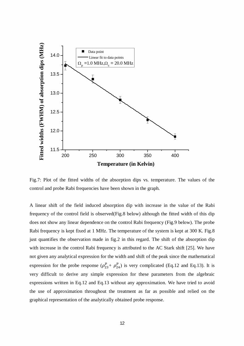
A plot of temperature vs. fitted width of the field induced absorption at fixed values of the

control and probe Rabi frequencies (훺 = 1 MHz, 훺 = 20 MHz) has been given in the figure

below (Fig.7) to establish that thermal broadening is indeed playing a vital role in generating

the line shape. The linear variation of the fitted width of the absorption dip with temperature

is seen. The effect of the thermal averaging on reducing the line width of the absorption dip is

thus confirmed. As usual, no shift of the absorption dip with temperature is found. Increase in

the ensemble temperature broadens the Doppler profile.

12

200 250 300 350 40011.5

12.0

12.5

13.0

13.5

14.0Data point Linear fit to data points

p =1.0 MHz,c = 20.0 MHz

Fitt

ed w

idth

s (FW

HM

) of a

bsor

ptio

n di

ps (M

Hz)

Temperature (in Kelvin)

Fig.7: Plot of the fitted widths of the absorption dips vs. temperature. The values of the

control and probe Rabi frequencies have been shown in the graph.

A linear shift of the field induced absorption dip with increase in the value of the Rabi

frequency of the control field is observed(Fig.8 below) although the fitted width of this dip

does not show any linear dependence on the control Rabi frequency (Fig.9 below). The probe

Rabi frequency is kept fixed at 1 MHz. The temperature of the system is kept at 300 K. Fig.8

just quantifies the observation made in fig.2 in this regard. The shift of the absorption dip

with increase in the control Rabi frequency is attributed to the AC Stark shift [25]. We have

not given any analytical expression for the width and shift of the peak since the mathematical

expression for the probe response (휌 + 휌 ) is very complicated (Eq.12 and Eq.13). It is

very difficult to derive any simple expression for these parameters from the algebraic

expressions written in Eq.12 and Eq.13 without any approximation. We have tried to avoid

the use of approximation throughout the treatment as far as possible and relied on the

graphical representation of the analytically obtained probe response.

13

10 20 30 40 50

0.0

0.5

1.0

1.5

2.0

2.5

3.0

3.5

4.0Data points Linear fit to data points

Shift

of t

he a

bsor

ptio

n di

p (M

Hz)

Control Rabi frequency (c) in MHz

Fig.8: A plot of the shift (in MHz) of the absorption dips vs. control Rabi frequency (in MHz)

at T = 300 K. The probe Rabi frequency is held fixed at 1 MHz throughout the simulation.

10 20 30 40 508

10

12

14

Fitt

ed a

bsor

ptio

n di

p w

idth

(FW

HM

in M

Hz)

Control Rabi frequency (c) in MHz

Data points Fit to data points

Fig.9: A plot of the fitted widths (FWHM in MHz) of the absorption dips vs. control Rabi

frequency (in MHz) at T = 300 K. Probe Rabi frequency is 1 MHz for all the data points.

14

A plot of the real part of (휌 + 휌 ) vs. probe detuning (훥 ) under both the Doppler free and

Doppler broadened regimes allows us to get an idea of the dispersive properties of the atomic

medium under the two different conditions. These are shown in Fig.10 and Fig.11 below. The

steepness of the dispersion at 훥 = 0 under the Doppler free condition decreases with the

increase in the Rabi frequency of the control field although under Doppler broadened

condition we expect modification in the dispersive behaviour of the atomic vapour. This

information will be useful to prepare a medium in which a sudden variation in the dispersive

property within a very short range is required. The intensity of the control field acting on the

energy levels of the atomic vapour system will be one of the main controlling factors of the

nature of the dispersion curve.

-400 -300 -200 -100 0 100-0.004

-0.003

-0.002

-0.001

0.000

0.001

0.002

0.003

0.004

-60 -40 -20 0 20 40 60-0.004

-0.003

-0.002

-0.001

0.000

0.001

0.002

0.003

0.004

Probe detuning in (p42) MHz

Re(p 23

p 24

)

Re(p 23

+ p 24

)

Probe detuning in (p42) MHz

c=10 MHz,

p=1MHz

c=20 MHz,

p=1MHz

c=30 MHz,

p=1MHz

c=40 MHz,

p=1MHz

c=50 MHz,

p=1MHz

Fig.10: Plot of R푒(휌 + 휌 ) vs. probe detuning (MHz) under Doppler free condition.

It is evident from the above figure that with increase in the Rabi frequency of the control field

the probe dispersion will get flatter and flatter. Under Doppler broadened regime the

steepness of the dispersion curve however decreases with increase in the Rabi frequency of

the control field, a feature just similar to that of Doppler free condition (please compare

15

Fig.10 and Fig.11). A kink like structure is appearing in the dispersion curve around the zero

probe field detuning (훥 = 0, fig. 11 below). This kink becomes prominent at higher

intensities of the control field. This has been shown in the inset of Fig.11 below. This kink

modulates the probe dispersion around zero probe detuning. This may have useful application

in studying the probe pulse propagation through such an atomic vapour system. This will be

quantified in a future correspondence.

-800 -600 -400 -200 0 200 400 600-0.0015

-0.0010

-0.0005

0.0000

0.0005

0.0010

0.0015

-40 -20 0 20 400.0000

0.0005

0.0010

Re(p 23

p 24

)

Probe detuning in (p42) MHz

Re(p 23

+ p 24

)

Probe detuning in (p42) MHz

c=10 MHz,p=1MHz

c=20 MHz,p=1MHz

c=30 MHz,p=1MHz

c=40 MHz,p=1MHz

c=50 MHz,p=1MHz

Fig.11: Plot of R푒(휌 + 휌 ) vs. probe detuning (in MHz) under Doppler broadened

conditions.

Till now we have been interested in studying the probe response under both the Doppler

broadened and Doppler free conditions by allowing the decay of the population from excited

level |3> to both the ground levels |1> and |2> but that from the level |4>has been restricted

only to level |2>. If the population from the state |4> is allowed to decay spontaneously to

both the ground levels we shall get alteration in the probe response. The appearance of the

absorption dip at and around the zero probe field detuning (훥 = 0) in the transparency

background as seen in Fig.2 will be absent at lower values of the Rabi frequency of the

16

control field. With increase in the Rabi frequency of the control field we can get back the

absorption dip at the same position but with lesser strength as compared to Fig.2. This has

been shown in the Fig.12 below.

-800 -600 -400 -200 0 200 400 600-0.0025

-0.0020

-0.0015

-0.0010

-0.0005

0.0000

-60 -40 -20 0 20 40 60-0.0020

-0.0015

-0.0010

-0.0005

Im(

p 23

p 24)

Probe detuning in (p42) MHz

c=10 MHz,

p=1MHz

c=20 MHz,

p=1MHz

c=30 MHz,

p=1MHz

c=40 MHz,

p=1MHz

c=50 MHz,

p=1MHz

Im(

p 23+ p 24

)

Probe detuning in (p42) MHz

Fig.12: Plot of imaginary part of the (휌 + 휌 )vs. probe frequency detuning (훥 ) under the

Doppler broadened regime (T = 300 K) with γ41 = 6 MHz. The values of the control (훺 ) and

probe (훺 ) Rabi frequencies have been mentioned in the figure.

In the inset of the above figure we have shown the zoomed probe response around zero probe

field detuning. If this is compared (Fig.13 below) with the zoomed part of Fig.2 we can see

that the absorption dip starts appearing when the Rabi frequency of the control field is

increased to 30 MHz and beyond but the absorption dips are not as prominent as in Fig.2. The

introduction of the extra decay channel in the theoretical model enhances the transparency by

diminishing the absorption at and around 훥 = 0. We can compare the field induced dips

formed in the background of the transparency window for both the cases with and without

nonzero contribution from γ41 under Doppler broadened regime.

17

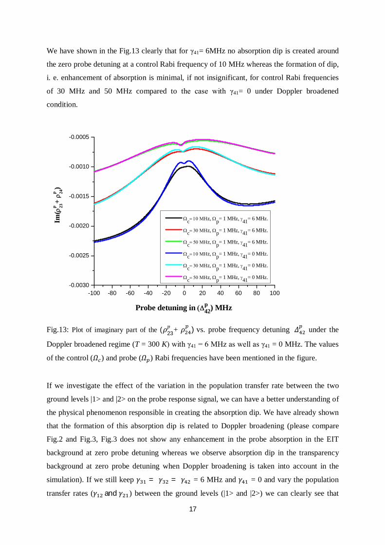
We have shown in the Fig.13 clearly that for γ41= 6MHz no absorption dip is created around

the zero probe detuning at a control Rabi frequency of 10 MHz whereas the formation of dip,

i. e. enhancement of absorption is minimal, if not insignificant, for control Rabi frequencies

of 30 MHz and 50 MHz compared to the case with γ41= 0 under Doppler broadened

condition.

-100 -80 -60 -40 -20 0 20 40 60 80 100-0.0030

-0.0025

-0.0020

-0.0015

-0.0010

-0.0005

Im(

p 23+ p 24

)

Probe detuning in (p42) MHz

cz, p= 1 MHz, 41= 6 MHz.

cz, p= 1 MHz, 41= 6 MHz.

cz, p= 1 MHz, 41= 6 MHz.

cz, p= 1 MHz, 41= 0 MHz.

cz, p= 1 MHz, 41= 0 MHz.

cz, p= 1 MHz, 41= 0 MHz.

Fig.13: Plot of imaginary part of the (휌23푝 + 휌 )vs. probe frequency detuning 훥 under the

Doppler broadened regime (T = 300 K) with γ41 = 6 MHz as well as γ41 = 0 MHz. The values

of the control (훺 ) and probe (훺 ) Rabi frequencies have been mentioned in the figure.

If we investigate the effect of the variation in the population transfer rate between the two

ground levels |1> and |2> on the probe response signal, we can have a better understanding of

the physical phenomenon responsible in creating the absorption dip. We have already shown

that the formation of this absorption dip is related to Doppler broadening (please compare

Fig.2 and Fig.3, Fig.3 does not show any enhancement in the probe absorption in the EIT

background at zero probe detuning whereas we observe absorption dip in the transparency

background at zero probe detuning when Doppler broadening is taken into account in the

simulation). If we still keep 훾 = 훾 = 훾 = 6 MHz and 훾 = 0 and vary the population

transfer rates (훾 and훾 ) between the ground levels (|1> and |2>) we can clearly see that

18

the dip appearing at the zero probe detuning is becoming more and more prominent with

increase in훾 . This is shown in the fig.14 below along with the statistics of fits in table-1.

For each of the graphs in Fig.14 we used훾 = 훾 .

-60 -40 -20 0 20 40 60-0.003

-0.002

-0.001

Im(

p 23+ p 24

)

Probe detuning in (p42) MHz

12=0.1MHz

12=0.3MHz

12=0.5MHz

12=0.7MHz

12

=0.9MHz 12=1.0MHz

Fig.14: Plot of imaginary part of the (휌23

푝 + 휌 )vs. probe frequency detuning(훥 ) under the

Doppler broadened regime (T = 300 K) with γ41 = 0 MHz. The values of the control (훺 ) and

probe (훺 ) Rabi frequencies have been kept fixed at 1 MHz and 30 MHz respectively. The

values of γ12 (population transfer rate from |1> to |2>) have been mentioned in the figure.

Table - 1

Population Transfer rate 훾 (from |1> to |2>) in MHz

Area under the absorption dip (in arb. unit)

Standard error of fit (Area)

Amplitude of the absorption dip (in arb. unit)

0.1 4.56467×10-4 6.68900×10-6 2.63097 ×10-5 0.3 5.92954 ×10-4 1.3208 0×10-5 4.06860 ×10-5 0.5 6.87988 ×10-4 1.39241 ×10-5 4.61169 ×10-5 0.7 7.33530 ×10-4 2.40127 ×10-5 4.79099 ×10-5 0.9 8.1815 0×10-4 4.0020 0×10-5 5.01683 ×10-5 1.0 8.9389 0×10-4 4.9221 0×10-5 5.2222 0×10-5

19

The availability of more atoms in the level |2> means these atoms would interact with the

coherent fields and thereby reduce the transparency at the zero probe detuning (under

Doppler broadened regime) when the population transfer rate from |1> to |2>is increased. In

the Fig.15 below we have also shown that the increase of the area under the absorption dip

with respect to 훾 is approximately linear. The values of the control and probe Rabi

frequencies have been kept fixed at 20 MHz and 1 MHz respectively.

0.2 0.4 0.6 0.8 1.00.0004

0.0006

0.0008

0.0010

Are

a un

der

the

abso

rptio

n di

p (in

arb

. uni

t)

Population transfer rate between |1> and |2> (

) (MHz)

Data point Linear fit to the data points

Fig.15: A linear fit to the plot of the area under the absorption dip (appearing around the zero

probe detuning) vs. 훾 . The values of the control and probe Rabi frequency used in the

simulation are 20 MHz and 1 MHz respectively.

4. Conclusion We have mainly shown here the effect of the addition of an extra ground level in a three-level

‘V’ type system and the role played by extra decay channels of the excited level population

on the probe response. The theoretical model has been developed to incorporate a probe field

coupling both the upper levels and a control field locked to a specific transition. The effect of

the inclusion and non-inclusion of different possible decay channels on the probe absorption

spectra has been shown under various conditions. The effect of Doppler broadening and the

formation of a field induced absorption signal on the background of a transparency window

on the probe response signal have been shown. The dependence of this field induced

20

absorption on various parameters like temperature, Rabi frequency of the control field etc.

has also been investigated in details. In fact, to the best of our knowledge, formation of an

absorption dip on the transparency background in a four-level ‘V’ type system is shown here

for the first time through a complete analytical treatment. The approach has been to

incorporate the experimental conditions to the closest possible way in the simulation. A

scheme is also presented on the basis of the outcome of this theoretical study for producing a

dispersive medium where rapid manipulation of the group velocity of the probe pulse

propagation can be achieved within a very small range of probe frequency detuning. The

model can also be used to study the effect of dephasing and other collision related population

transfer phenomena among the ground levels on the probe response. We believe that this

simple analytical model will be useful in probing the ‘V’ type system in further details in the

future and exciting new results can be obtained.

Acknowledgements: AB acknowledges Department of Science & Technology (DST), New

Delhi for granting a research project under the start-up research grant (Young Scientists)

(sanction order no. SR/FTP/PS-079/2010, dated: 14/08/2013) and the University Grants

Commission (UGC), New Delhi for granting a major research project (F. No. – 43-

527/2014(SR) dated: 28/09/2015). DB thanks the University Grants Commission (UGC) for a

research project (Sanction order no. F PSW-205/13-14 dated 01/08/2014). KI and AG

acknowledge Visva-Bharati for providing research fellowship. The authors thank Prof.

Swapan Mandal (Department of Physics, Visva-Bharati) for sharing his experiences and

resources.

References:

1. K-J Boller, A. Imamoglu and S.E. Harris, Phys. Rev. Lett. 66 2593 (1991).

2. S.E. Harris, Phys. Today 50 36 (1997).

3. G. Alzetta, L. Moi and G. Orriols, Nuovo Cimento B 52 209 (1979).

4. F. Magnus, A.L. Boatwright, A. Flodinand and R.C. Shiell, J. Opt. B: Quantum

Semiclass. Opt.7 109 (2005).

5. S. Chakrabarti, A. Pradhan, B. Ray and P.N. Ghosh, J. Phys. B: At. Mol. Opt. Phys.

38 4321 (2005).

6. J. Clarke, H. Chen and A. Van Wijngaarden, Appl. Opt. 40 2047 (2001).

7. A. Ray, Md. S. Ali and A. Chakrabarti, Opt. Laser. Technol. 60 107 (2014).

8. I. Novikova, D.F. Phillips and R.L. Walsworth, Phys. Rev. Lett. 99 173604 (2007).

21

9. A. Joshi and M. Xiao, Phys. Lett. A 317 370 (2003).

10. L. Zhang, F. Zhou, Y. Niu, J. Zhang and S. Gong, Opt. Commun.284 5697 (2011).

11. K. Pandey, Phys. Rev. A 87 043838 (2013).

12. L.B. Kong, X.H. Tu, J. Wang, Y. Zhu and M.S. Zhan, Opt. Commun. 269 362 (2007).

13. A. Fleischhauer and M.D. Lukin, Phys. Rev. Lett. 84, 5094 (2000).

14. D.F. Phillips, A. Fleischhauer, A. Mair A and R.L. Walsworth, Phys. Rev. Lett. 86

783 (2001).

15. D.J. Fulton, S. Shepherd, R.R. Moseley, B.D. Sinclair and M.H. Dunn, Phys. Rev. A

52 2302 (1995).

16. S.M. Iftiquar, G.R. Karve and V. Natarajan, Phys. Rev. A 77 063807 (2008).

17. D. Bhattacharyya, A. Ghosh, A. Bandyopadhyay, S. Sahaand S. De, J. Phys. B At.

Mol. Opt. Phys.48 175503 (2015).

18. H.H. Kim, M.H. Ahn, K. Kim, J.B. Kim and H.S. Moon, J. Korean Phy. Soc. 46 1109

(2005).

19. S.R. Chanu, K. Pandey and V. Natarajan, Euro Phys. Lett.9844009 (2012).

20. D.A. Steck, Rubidium 87 D line data (2009) http://steck.us/alkalidata.

21. S.C. Rand, Lectures on Light - Nonlinear and Quantum Optics using the Density

Matrix, 1st Ed. (Oxford University Press, 2010), ISBN No. 978-0-19-957487-2.

22. M.O. Scully and M.S. Zubairy M, Quantum Optics (London: Cambridge University

Press, 1997).

23. W. Demtroder, Laser Spectroscopy: 2nd Ed. Springer-Verlag.

24. M. A. Kumar and S. Singh, Phys. Rev. A 87 065801 (2013).

25. C. Wei, D. Suter, A.S.M. Windsor and N.B. Manson, Phys. Rev. A 58 2310 (1998).