Formalization of Discret-Time Markov Chains in HOL

Liya Liu, Osman Hasan, and Sofiene Tahar

Department of Electrical and Computer Engineering,Concordia University, Montreal, Canada

liy liu,o hasan,tahar@ece.concordia.ca

Technical Report April 2011

Abstract

The mathematical concept of Markov chains is widely used to model and analyze many engineering

and scienti?c problems. Markovian models are usually analyzed using computer simulation, and more

recently using probabilistic model-checking but these methods either do not guarantee accurate analysis

or are not scalable. As an alternative, we propose to use higher-order-logic theorem proving to reason

about properties of systems that can be described as Markov chains. As the ?rst step towards this goal,

this paper presents a formalization of time homogeneous ?nite-state Discrete-time Markov chains and

the formal veri?cation of some of their fundamental properties, such as Joint probabilities, Chapman

Kolmogorov equation and steady state probabilities, using the HOL theorem prover. For illustration

purposes, we utilize our formalization to analyze a simpli?ed binary communication channel.

1

In probability theory, Markov chains are used to model time varying random phenomenathat exhibit the memoryless property [3]. In fact, most of the randomness that we encounterin engineering and scientific domains has some sort of time-dependency. For example, noisesignals vary with time, duration of a telephone call is somehow related to the time it is made,population growth is time dependant and so is the case with chemical reactions. Therefore,Markov chains have been extensively investigated and applied for designing systems in manybranches of science and engineering. Some of their important applications include functionalcorrectness and performance analysis of telecommunication and security protocols, relia-bility analysis of hardware circuits, software testing, internet page ranking and statisticalmechanics.

Traditionally, simulation has been the most commonly used computer-based analysis tech-nique for Markovian models. The approximate nature of simulation poses a serious prob-lem in highly sensitive and safety critical applications, such as, nuclear reactor control andaerospace software engineering. To improve the accuracy of the simulation results, MarkovChain Monte Carlo (MCMC) methods [15], which involve sampling from desired probabilitydistributions by constructing a Markov chain with the desired distribution, are frequentlyapplied. The major limitation of MCMC is that it generally requires hundreds of thousandsof simulations to evaluate the desired probabilistic quantities and becomes impractical wheneach simulation step involves extensive computations. Other state-based approaches to an-alyze Markovian models include software packages, such as Markov analyzers and reliabilityor performance evaluation tools, which are all based on numerical methods [26]. Althoughthese software packages can be successfully applied to analyze large scale Markovian models,the results cannot be guaranteed to be accurate because the underlying iterative methodsare not 100% precise. Another technique, Stochastic Petri Nets (SPN ) [9], has been foundas a powerful method for modeling and analyzing Markovian systems because it allows localstate modeling instead of global modeling. The key limiting factor of the application of SPNmodels using this approach is the complexity of their analysis.

Formal methods are able to conduct precise system analysis and thus overcome the inac-curacies of the above mentioned techniques. Due to the extensive usage of Markov chainsin analyzing safety-critical systems, probabilistic model checking [23] has been recently pro-posed for analyzing Markov chains. It offers exact solutions but is limited by the state-spaceexplosion problem [2] and the time of analyzing a system is largely dependent on the conver-gence speed of the underlying algorithms. Similarly, we cannot verify generic mathematicalproperties using probabilistic model checking due to the inherent state-based nature of theapproach. Thus, the probabilistic model checking approach, even though is capable of pro-viding exact solutions automatically, is quite limited in terms of handling a variety of systemsand properties.

In this paper, we propose to use higher-order-logic theorem proving [7] as a complemen-tary technique for analyzing Markovian models and thus overcome the limitations of theabove mentioned techniques. Time-homogeneousity is an important concept in analyzingMarkovian models. In particular, we formalize a time-homogeneous Discrete-Time MarkovChain (DTMC) with finite state space in higher-order logic and then, building upon thisdefinition, formally verify some of the fundamental properties of a DTMC, such as, JointProbability Distribution, Chapman-Kolmogorov Equation, and Steady-state Probabilities [3].These properties play a vital role in reasoning about many interesting characteristics whileanalyzing the Markovian models of real-world systems as well as pave the path to the verifi-cation of more advanced properties related to DTMC. In order to illustrate the effectivenessof our work and demonstrate its utilization, we present the formal analysis of a simplified

2

binary communication channel.

1 Related Work

As described above, Markov Analyzers, such as MARCA [16] and DNAmaca [14], whichcontain numerous matrix manipulation and numerical solution procedures, are powerfulautonomous tools for analyzing large-scale Markovian models. Unfortunately, most of theiralgorithms are based on iterative methods that begin from some initial approximation andend at some convergent point, which is the main source of inaccuracy in such methods.

Many reliability evaluation software tools integrate simulation and numerical analyzersfor modeling and analyzing the reliability, maintainability or safety of systems using Markovmethods, which offer simplistic modeling approaches and are more flexible compared totraditional approaches, such as Fault Tree [5]. Some prevalent tool examples are Mobius [18]and Relex Markov [?]. Some other software tools for evaluating performance, e.g. MACOM[24] and HYDRA [19], take the advantages of a popular Markovian algebra, i.e., PEPA[21], to model systems and efficiently compute passage time densities and quantities inlarge-scale Markov chains. However, the algorithms used to solve the models are based onapproximations, which leads to inaccuracies.

Stochastic Petri Nets provide a versatile modeling technique for stochastic systems. Themost popular softwares are SPNP [4] and GreatSPN [8]. These tools can model, validate,and evaluate the distributed systems and analyze the dynamic events of the models usingsomething other than the exponential distribution. Although they can easily manage the sizeof the system model, the iterative methods employed to compute the stationary distributionor transient probabilities of a model result in inaccurate analysis.

Probabilistic model checking [1, 23] is the state-of-the-art formal Markov chain analysistechnique. Numerous probabilistic model checking algorithms and methodologies have beenproposed in the open literature, e.g., [6, 20], and based on these algorithms, a number oftools, e.g., PRISM [22] and VESTA [25] have been developed. They support the analysis ofprobabilistic properties of DTMC, Continuous-Time Markov chains, Markov decision pro-cesses and Semi-Markov Process and have been used to analyze many real-world systemsincluding communication and multimedia protocols. But they suffer from state-space explo-sion as well as do not support the verification of generic mathematical expressions. Also,because of numerical methods implemented in the tools, the final results cannot be termed100% accurate. The proposed HOL theorem proving based approach provides another wayto specify larger systems and accurate results.

HOL theorem proving has also been used for conducting formal probabilistic analysis.Hurd [13] formalized some measure theory in higher-order logic and proposed an infras-tructure to formalize discrete random variables in HOL. Then, Hasan [10] extended Hurd’swork by providing the support to formalize continuous random variables [10] and verify thestatistical properties, such as, expectation and variance, for both discrete and continuousrandom variables [10, 11]. Recently, Mhamdi [17] proposed a significant formalization of mea-sure theory and proved Lebesgue integral properties and convergence theorems for arbitraryfunctions. But, to the best of our knowledge, the current state-of-the-art high-order-logictheorem proving based probabilistic analysis do not provide any theory to model and verifyMarkov systems and reasoning about their corresponding probabilistic properties. The maincontribution of the current paper is to bridge this gap. We mainly build upon Hurd’s workto formalize DTMC and verify some of their basic probabilistic properties. The main reasonbehind choosing Hurd’s formalization of probability theory for our work is the availability of

3

formalized discrete and continuous random variables in this framework, as described above.These random variables can be utilized along with our formalization of DTMC to formallyrepresent real-world systems by their corresponding Markovian models in higher-order logicand reason about these models in a higher-order-logic theorem prover.

2 Probability Theory and Random Variables in HOL

A measure space is defined as a triple (Ω,Σ, µ) where Ω is a set, called the sample space, Σrepresents a σ-algebra of subsets of Ω and the subsets are usually referred to as measurablesets, and µ is a measure with domain Σ. A probability space is a measure space (Ω,Σ,Pr)such that the measure, referred to as the probability and denoted by Pr, of the sample spaceis 1.

The measure theory developed by Hurd [13] defines a measure space as a pair (Σ, µ).Whereas the sample space, on which this pair is defined, is implicitly implied from thehigher-order-logic definitions to be equal to the universal set of the appropriate data-type.Building upon this formalization, the probability space was also defined in HOL as a pair(E ,P), where the domain of P is the set E , which is a set of subsets of infinite Booleansequences B∞. Both P and E are defined using the Caratheodory’s Extension theorem,which ensures that E is a σ-algebra: closed under complements and countable unions.

Now, a random variable, which is one of the core concepts in probabilistic analysis, isa fundamental probabilistic function and thus can be modeled in higher-order logic as adeterministic function, which accepts the infinite Boolean sequence as an argument. Thesedeterministic functions make random choices based on the result of popping the top mostbit in the infinite Boolean sequence and may pop as many random bits as they need fortheir computation. When the functions terminate, they return the result along with theremaining portion of the infinite Boolean sequence to be used by other programs. Thus, arandom variable which takes a parameter of type α and ranges over values of type β can berepresented in HOL by the following function.

F : α→ B∞ → β ×B∞

As an example, consider a Bernoulli(12) random variable that returns 1 or 0 with equal

probability 12 . It has been formalized in higher-order logic as follows

∀ s. bit s = if shd s then 1 else 0, stl s

where the functions shd and stl are the sequence equivalents of the list operations ’head’ and’tail’, respectively. The function bit accepts the infinite Boolean sequence s and returns apair. The first element of the returned pair is a random number that is either 0 or 1,depending on the Boolean value of the top most element of s. Whereas, the second elementof the pair is the unused portion of the infinite Boolean sequence, which in this case is thetail of the sequence.

Once random variables are formalized, as mentioned above, we can utilize the formalizedprobability theory infrastructure to reason about their probabilistic properties. For example,the following Probability Mass Function (PMF) property can be verified for the function bit

using the HOL theorem prover.

` P s | FST (bit s) = 1 = 12

4

where the function FST selects the first component of a pair and x|C(x) represents a setof all x that satisfy the condition C.

The above approach has been successfully used to formally verify most basic probabilitytheorems [13], such as the law of additivity, and conditional probability related properties[12]. For instance, the conditional probability has been formalized as:

Definition: Conditional Probability` ∀ A B.

cond prob A B = P(A⋂

B) / P(B)which plays a vital role in our work. Another frequently used formally verified theorem, inour work, is the Total Probability Theorem [12], which is described, for a finite, mutuallyexclusive, and exhaustive sequence Bi of events and an event A, as follows

Pr(A) =

n−1∑i=0

Pr(Bi)Pr(A|Bi). (1)

We also verified the following closely related property in HOL

Pr(B)Pr(A|B) = Pr(A)Pr(B|A) (2)

where events A and B are measurable. This property will be used in verifying some importantMarkov chain properties later.

3 Formal Modeling of Discrete-Time Markov Chains

Given a probability space, a stochastic process Xt : Ω → S represents a sequence ofrandom variables X, where t represents the time that can be discrete (represented by non-negetive integers) or continuous (represented by real numbers) [3]. The set of values takenby each Xt, commonly called states, is referred to as the state space. The sample space Ω ofthe process consists of all the possible sequences based on a given state space S. Now, basedon these definitions, a Markov process can be defined as a stochastic process with Markovproperty. If a Markov process has finite or countably infinite state space, then it is called aMarkov chain and satisfies the following Markov property.

For all k and p, if p < t, k < p and xt+1 and all the states xi (i ∈ [k, t)) are in the statespace, then

PrXt+1 = xt+1|Xt = xt, . . . , Xp = xp . . . , Xk = xk =

PrXt+1 = xt+1|Xt = xt.(3)

Additionally, if t ranges over nonnegative integers or, in other words, the time is a discretequantity, and the states are in a finite state space, then such a Markov chain is called aFinite-state Discrete-Time Markov Chain. A Markov chain, if with the same conditionalprobabilities Pr(Xn+1 = a | Xn = b), is referred to as the time-homogeneous Markov chain[3]. Time-homogeneousity is an important concept in analyzing Markovian models andtherefore, in our development, we focus on formalizing Time-homogeneous Discrete-TimeMarkov Chain with finite space, which we refer to in this paper as DTMC. A DTMC isusually expressed by specifying:

• an initial distribution defined by π0(s) = Pr(X0 = s), π0(s) ≥ 0(∀s ∈ S), and∑s∈S π0(s) = 1.

5

• transition probabilities pij defined as ∀i, j ∈ S, pij = PrXt+1 = j|Xt = i, pij ≥ 0and

∑j∈S pij = 1

Based on the above mentioned definitions, we formalize the notion of a DTMC in HOLas the following predicate:

Definition 1:Time homogeneous Discrete-Time Markov Chain with Finite state space` ∀ f l x Linit Ltrans.

Time homo mc f l x Linit Ltrans =

(∀ i. (i < l) ⇒(Ps | FST (f 0 s) = xi = EL i Linit) ∧(∑l−1

k=0(EL i Linit = 1))) ∧(∀ t i j. (i < l) ∧ (j < l) ⇒

(Ps | FST (f (t + 1) s) = xj|s | FST (f t s) = xi =

(EL (i * l + j) Ltrans)) ∧(∑l−1

k=0(EL (i * l + k) Ltrans = 1))) ∧(∀ t k. (k < l) ⇒ measurable s | FST (f t s) = xk) ∧(∀ t.

⋃l−1k=0 s | FST (f t s) = xk = UNIV) ∧

(∀ t u v. (u < l) ∧ (v < l) ∧ (u 6= v) ⇒disjoint (s | FST (f t s) = xu s | FST (f t s) = xv)) ∧

(∀ i j m r t w L Lt.

((∀ k. (k ≤ r) ⇒ (EL k L < l)) ∧ (i < l) ∧ (j < l) ∧(Lt ⊆ [m, r]) ∧ (m ≤ r) ∧ (w + r < t)) ⇒(P(s | FST (f (t + 1) s) = xj|s | FST (f t s) = xi

⋂(⋂kεLt s | FST (f (w + k) s) = x(EL k L))) =

P(s | FST (f (t + 1) s) = xj|s | FST (f t s)= xi))) ∧(∀ t n i j.

(i < l) ∧ (j < l) ⇒(P(s | FST (f (t + 1) s) = xj|s | FST (f t s) = xi) =

P(s | FST (f (n + 1) s) = xj|s | FST (f n s) = xi)))

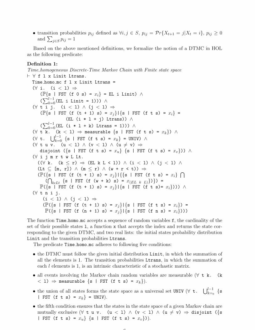
The function Time homo mc accepts a sequence of random variables f, the cardinality of theset of their possible states l, a function x that accepts the index and returns the state cor-responding to the given DTMC, and two real lists: the initial states probability distributionLinit and the transition probabilities Ltrans.

The predicate Time homo mc adheres to following five conditions:

• the DTMC must follow the given initial distribution Linit, in which the summation ofall the elements is 1. The transition probabilities Ltrans, in which the summation ofeach l elements is 1, is an intrinsic characteristic of a stochastic matrix.

• all events involving the Markov chain random variables are measurable (∀ t k. (k

< l) ⇒ measurable s | FST (f t s) = xk).

• the union of all states forms the state space as a universal set UNIV (∀ t.⋃l−1k=0s

| FST (f t s) = xk = UNIV).

• the fifth condition ensures that the states in the state space of a given Markov chain aremutually exclusive (∀ t u v. (u < l) ∧ (v < l) ∧ (u 6= v) ⇒ disjoint (s| FST (f t s) = xu s | FST (f t s) = xv)).

6

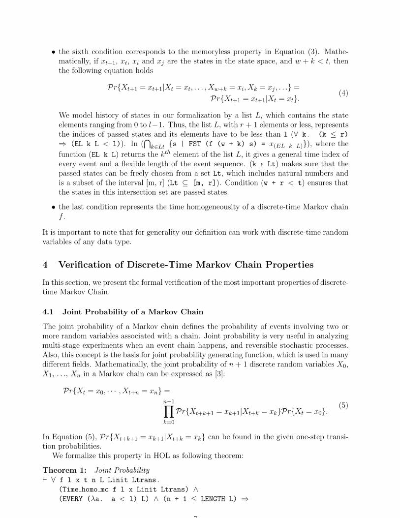
• the sixth condition corresponds to the memoryless property in Equation (3). Mathe-matically, if xt+1, xt, xi and xj are the states in the state space, and w + k < t, thenthe following equation holds

PrXt+1 = xt+1|Xt = xt, . . . , Xw+k = xi, Xk = xj , . . . =

PrXt+1 = xt+1|Xt = xt.(4)

We model history of states in our formalization by a list L, which contains the stateelements ranging from 0 to l−1. Thus, the list L, with r + 1 elements or less, representsthe indices of passed states and its elements have to be less than l (∀ k. (k ≤ r)

⇒ (EL k L < l)). In (⋂k∈Lt s | FST (f (w + k) s) = x(EL k L)), where the

function (EL k L) returns the kth element of the list L, it gives a general time index ofevery event and a flexible length of the event sequence. (k ε Lt) makes sure that thepassed states can be freely chosen from a set Lt, which includes natural numbers andis a subset of the interval [m, r] (Lt ⊆ [m, r]). Condition (w + r < t) ensures thatthe states in this intersection set are passed states.

• the last condition represents the time homogeneousity of a discrete-time Markov chainf .

It is important to note that for generality our definition can work with discrete-time randomvariables of any data type.

4 Verification of Discrete-Time Markov Chain Properties

In this section, we present the formal verification of the most important properties of discrete-time Markov Chain.

4.1 Joint Probability of a Markov Chain

The joint probability of a Markov chain defines the probability of events involving two ormore random variables associated with a chain. Joint probability is very useful in analyzingmulti-stage experiments when an event chain happens, and reversible stochastic processes.Also, this concept is the basis for joint probability generating function, which is used in manydifferent fields. Mathematically, the joint probability of n + 1 discrete random variables X0,X1, . . ., Xn in a Markov chain can be expressed as [3]:

PrXt = x0, · · · , Xt+n = xn =

n−1∏k=0

PrXt+k+1 = xk+1|Xt+k = xkPrXt = x0.(5)

In Equation (5), PrXt+k+1 = xk+1|Xt+k = xk can be found in the given one-step transi-tion probabilities.

We formalize this property in HOL as following theorem:

Theorem 1: Joint Probability` ∀ f l x t n L Linit Ltrans.

(Time homo mc f l x Linit Ltrans) ∧(EVERY (λa. a < l) L) ∧ (n + 1 ≤ LENGTH L) ⇒

7

P(⋂nk=0s | FST (f (t + k) s) = x(EL k L)) =∏n−1

k=0P(s | FST (f (t + k + 1) s) = x(EL (k+1) L)|s | FST (f (t + k) s) = x(EL k L))

Ps | FST (f t s) = x(EL 0 L)

The variables above are used in the same context as Definition 1. The first assumptionensures that f is a Markov chain. All the elements of the indices sequence L are less thanl and the length of L is larger than or equal to the length of the segment considered in thejoint events. The conclusion of the theorem represents Equation (5) in higher-order logicbased on the probability theory formalization, presented in Section 2. The proof of Theorem1 is based on induction on the variable n, Equation (1) and some arithmetic reasoning.

4.2 Chapman-Kolmogorov Equation

The well-known Chapman-Kolmogorov equation [3] is a widely used property of time ho-mogeneous Markov chains as it facilitates the use of a matrix theory for analyzing largeMarkov chains. It basically gives the probability of going from state i to j in m + n steps.Assuming the first m steps take the system from state i to some intermediate state k, whichis in the state space Ω and the remaining n steps then take the system from state k to j,we can obtain the desired probability by adding the probabilities associated with all theintermediate steps.

pij(m+ n) =∑k∈Ω

pkj(n)pik(m) (6)

The notation pij(n) denotes the n-step transition probabilities from state i to j.

pij(n) = PrXt+n = xj |Xt = xi (7)

Based on Equation (6), and Definition 1, the Chapman-Kolmogorov equation is formalizedas follows

Theorem 2: Chapman-Kolmogorov Equation` ∀ f i j x l m n Linit Ltrans.

(Time homo mc f l x Linit Ltrans) ∧ (i < l) ∧ (j < l) ∧(∀ r. (r < l) ⇒ (0 < Ps | FST (f 0 s) = xr)) ⇒P(s | FST (f (m + n) s) = xj|s | FST (f 0 s) = xi) =∑l−1

k=0(P(s | FST (f n s) = xj|s | FST (f 0 s) = xk)P(s | FST (f m s) = xk|s | FST (f 0 s) = xi))

The variables m and n denote the steps between two states and both of them represent time.The first assumption ensures that the random process f is a time homogeneous DTMC, usingDefinition 1. The following two assumptions, i < l and j < l, define the allowable bounds forthe index variables. The last assumption is used to exclude the case when PrX0 = xj = 0.Because it makes no sense to analyze the conditional probability when the probability of astate existing is 0. The conclusion of the theorem formally represents Equation (6).

The proof of Theorem 2 again involves induction on the variable n and both of the baseand step cases are discharged using the following lemma.

Lemma 1: Multistep Transition Probability` ∀ f i j x n Linit Ltrans.

8

(Time homo mc f l x Linit Ltrans) ∧ (i < l) ∧ (j < l) ∧(0 < Ps | FST (f 0 s) = xi) ⇒P(s | FST (f (n + 1) s) = xj|s | FST (f 0 s) = xi) =∑l−1

k=0P(s | FST (f 1 s) = xj|s | FST (f 0 s) = xk)P(s | FST (f n s) = xk|s | FST (f 0 s) = xi)

The proof of Lemma 1 is primarily based on the Total Probability theorem (1).

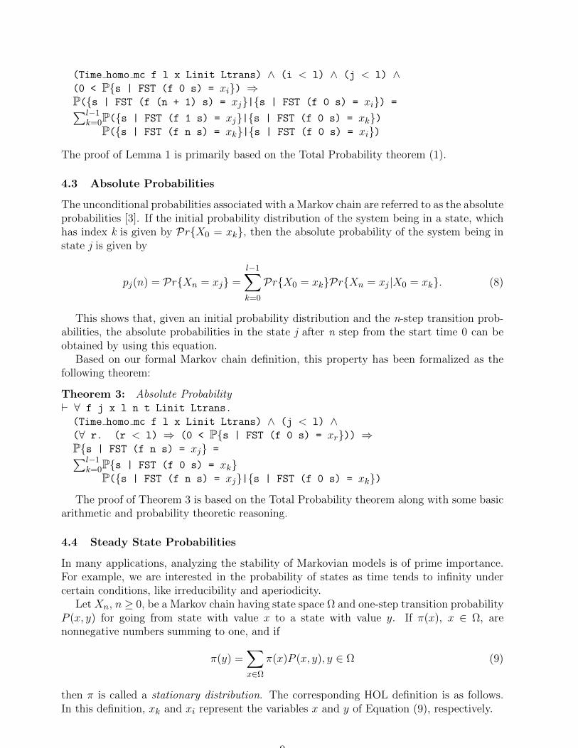
4.3 Absolute Probabilities

The unconditional probabilities associated with a Markov chain are referred to as the absoluteprobabilities [3]. If the initial probability distribution of the system being in a state, whichhas index k is given by PrX0 = xk, then the absolute probability of the system being instate j is given by

pj(n) = PrXn = xj =

l−1∑k=0

PrX0 = xkPrXn = xj |X0 = xk. (8)

This shows that, given an initial probability distribution and the n-step transition prob-abilities, the absolute probabilities in the state j after n step from the start time 0 can beobtained by using this equation.

Based on our formal Markov chain definition, this property has been formalized as thefollowing theorem:

Theorem 3: Absolute Probability` ∀ f j x l n t Linit Ltrans.

(Time homo mc f l x Linit Ltrans) ∧ (j < l) ∧(∀ r. (r < l) ⇒ (0 < Ps | FST (f 0 s) = xr)) ⇒Ps | FST (f n s) = xj =∑l−1

k=0Ps | FST (f 0 s) = xkP(s | FST (f n s) = xj|s | FST (f 0 s) = xk)

The proof of Theorem 3 is based on the Total Probability theorem along with some basicarithmetic and probability theoretic reasoning.

4.4 Steady State Probabilities

In many applications, analyzing the stability of Markovian models is of prime importance.For example, we are interested in the probability of states as time tends to infinity undercertain conditions, like irreducibility and aperiodicity.

Let Xn, n ≥ 0, be a Markov chain having state space Ω and one-step transition probabilityP (x, y) for going from state with value x to a state with value y. If π(x), x ∈ Ω, arenonnegative numbers summing to one, and if

π(y) =∑x∈Ω

π(x)P (x, y), y ∈ Ω (9)

then π is called a stationary distribution. The corresponding HOL definition is as follows.In this definition, xk and xi represent the variables x and y of Equation (9), respectively.

9

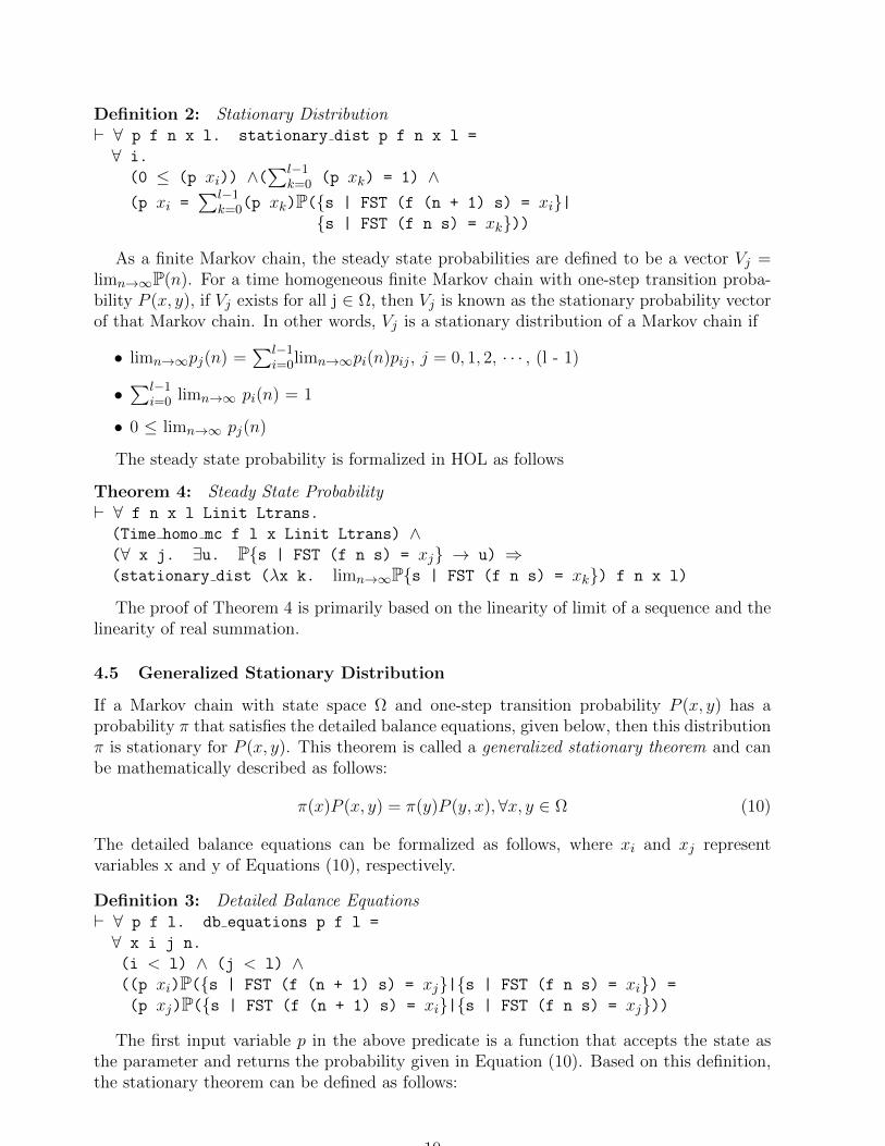
Definition 2: Stationary Distribution` ∀ p f n x l. stationary dist p f n x l =

∀ i.

(0 ≤ (p xi)) ∧(∑l−1

k=0 (p xk) = 1) ∧(p xi =

∑l−1k=0(p xk)P(s | FST (f (n + 1) s) = xi|

s | FST (f n s) = xk))

As a finite Markov chain, the steady state probabilities are defined to be a vector Vj =limn→∞P(n). For a time homogeneous finite Markov chain with one-step transition proba-bility P (x, y), if Vj exists for all j ∈ Ω, then Vj is known as the stationary probability vectorof that Markov chain. In other words, Vj is a stationary distribution of a Markov chain if

• limn→∞pj(n) =∑l−1

i=0limn→∞pi(n)pij , j = 0, 1, 2, · · · , (l - 1)

•∑l−1

i=0 limn→∞ pi(n) = 1

• 0 ≤ limn→∞ pj(n)

The steady state probability is formalized in HOL as follows

Theorem 4: Steady State Probability` ∀ f n x l Linit Ltrans.

(Time homo mc f l x Linit Ltrans) ∧(∀ x j. ∃u. Ps | FST (f n s) = xj → u) ⇒(stationary dist (λx k. limn→∞Ps | FST (f n s) = xk) f n x l)

The proof of Theorem 4 is primarily based on the linearity of limit of a sequence and thelinearity of real summation.

4.5 Generalized Stationary Distribution

If a Markov chain with state space Ω and one-step transition probability P (x, y) has aprobability π that satisfies the detailed balance equations, given below, then this distributionπ is stationary for P (x, y). This theorem is called a generalized stationary theorem and canbe mathematically described as follows:

π(x)P (x, y) = π(y)P (y, x), ∀x, y ∈ Ω (10)

The detailed balance equations can be formalized as follows, where xi and xj representvariables x and y of Equations (10), respectively.

Definition 3: Detailed Balance Equations` ∀ p f l. db equations p f l =

∀ x i j n.

(i < l) ∧ (j < l) ∧((p xi)P(s | FST (f (n + 1) s) = xj|s | FST (f n s) = xi) =

(p xj)P(s | FST (f (n + 1) s) = xi|s | FST (f n s) = xj))

The first input variable p in the above predicate is a function that accepts the state asthe parameter and returns the probability given in Equation (10). Based on this definition,the stationary theorem can be defined as follows:

10

1

1

Fig. 1: State Diagram and Channel Diagram of the Binary Channel Model

Theorem 5: Generalized Stationary Distribution` ∀ f x l n Linit Ltrans.

(db equations (λx i. Ps | FST (f n s) = xi) f l) ∧(Time homo mc f l x Linit Ltrans) ⇒(stationary dist (λx k. Ps | FST (f n s) = xk) f n x l)

Here, π(x) is specified as a function λx i. Ps | FST (f n s) = xi. The proof of Theorem 5is based on the Total Probability theorem, given in Equation (1), and the following Lemma:

Lemma 3: Summation of Transition Probability` ∀ f x l i n Linit Ltrans.

(Time homo mc f l x Linit Ltrans) ∧ (i < l) ⇒∑l−1j=0P(s | FST (f n s) = xj|s | FST (f 0 s) = xi = 1

The proof script1for the formalization of Markov chain, presented in this section, consistsof approximately 2600 lines of HOL code. These results not only ensure the correctness ofour formal Markov chain definitions, presented in Section 3, but also play a vital role inanalyzing real-world systems that are modeled by DTMC, as will be demonstrated in thenext section.

5 Application: Binary Communication Channel

In order to illustrate the usefulness of the proposed approach, we use our results to analyzea simplified binary communication channel model [27]. Also, we compare the analysis of thesame example using probabilistic model checking.

A binary communication channel is a channel with binary inputs and outputs. Thetransmission channel is assumed to be noisy or imperfect, i.e., it is likely that the receivergets the wrong digit. This channel can be modeled as a two-state time homogenous DTMCwith the following state transition probabilities.

PrXn+1 = 0 | Xn = 0 = 1 - a; PrXn+1 = 1 | Xn = 0 = a;

PrXn+1 = 0 | Xn = 1 = b; PrXn+1 = 1 | Xn = 1 = 1 - b

The corresponding state diagram and channel diagram are given in Fig. 1. The binarycommunication channel is widely used in telecommunication theory as more complicatedchannels are modeled by cascading several of them. Here, variables Xn−1 and Xn denotethe digits leaving the systems (n − 1)th stage and entering the nth one, respectively. a andb are the crossover bit error probabilities. Because variables X0 is also a random variable,the initial state is not determined, Pr (X0 = 0) and Pr (X0 = 1) could not be 0 or 1.

Although the initial distribution is unknown, the given binary communication channelhas been formalized in HOL as a generic model, using Definition 2.

1Available at http://users.encs.concordia.ca/∼liy liu/code.html

11

Definition 4: Binary Communication Channel Model` ∀ f x a b p q.

(binary communication channel model f a b p q) =

(Time homo mc f (2:num) x [p; q] [1 - a; a; b; 1 - b]) ∧(|1 - a - b| < 1) ∧ (0 ≤ a ≤ 1) ∧ (0 ≤ b ≤ 1) ∧(p + q = 1) ∧ (0 < p < 1) ∧ (0 < q < 1)

In this formal model, variable f represents the Markov chain and variables a, b, p andq are parameters of the functions of initial distribution and transition probabilities. Thevariable x represents a function that provides the state at a given index.

The first condition ensures that f is a time-homogeneous DTMC, with which the numberof states l is 2, because there are only two states in the state space. List [p; q] correspondsto Linit in Definition 1 and another list [1 - a; a; b; 1 - b] gives the one-step transi-tion probability matrix by combining all the rows into a list and corresponds to Ltrans inDefinition 1. The next three conditions define the allowable intervals for parameters a andb to restrict the probability terms in [0,1]. It is important to note that, |1 - a - b| <

1 ensures that both a and b cannot be equal to 0 and 1 at the same time and thus avoidsthe zero transition probabilities. The remaining conditions correspond to one-step transitionprobabilities.

Next, we use our formal model to reason about the following properties.

Theorem 6: nth step Transition Probabilities` ∀ f x a b n p q.

(binary communication channel model f x a b p q) ⇒(P(s|FST (f n s)=x0|s|FST (f 0 s))=x0)= b+a(1−a−b)n

a+b ) ∧(P(s|FST (f n s)=x1|s|FST (f 0 s))=x0)=a−a(1−a−b)n

a+b ) ∧(P(s|FST (f n s)=x0|s|FST (f 0 s))=x1)= b−b(1−a−b)

n

a+b ) ∧(P(s|FST (f n s)=x1|s|FST (f 0 s))=x1)=a+b(1−a−b)n

a+b )

Theorem 7: Limiting State Probabilities` ∀ f x a b p q.

(binary communication channel model f x a b p q) ⇒(limn→∞P(s|FST (f n s)=x0|s|FST (f 0 s))=x0)= b

a+b) ∧(limn→∞P(s|FST (f n s)=x1|s|FST (f 0 s))=x0)= a

a+b) ∧(limn→∞P(s|FST (f n s)=x0|s|FST (f 0 s))=x1)= b

a+b) ∧(limn→∞P(s|FST (f n s)=x1|s|FST (f 0 s))=x1)= a

a+b)

Theorem 6 has been verified by performing induction on n and then applying Theorem 2and Lemma 3 and along with some arithmetic reasoning. Theorem 6 is then used to verifyTheorem 7 along with limit of real sequence principles.

Now, we modeled the binary communication channel in the PRISM probabilistic modelchecker and tried to evaluate the same nth-step transition probabilities, given in Theorems4 to 7. For this purpose, we have to specify exact values for probabilities a and b and thenumber of steps n. We experimented by sweeping variables a and b in the interval [0; 1]with a step size 0.1, and setting n = 4. The results are depicted graphically in Figure 2.

This small case study clearly illustrates the main strength of the proposed theorem prov-ing based technique against the probabilistic model checking approach. In the proposedapproach, we verified the desired probabilistic characteristics as generic theorems that are

12

Fig. 2: The 4-step transition probabilities with resolution 0.1

universally quantified for all allowable values of variables a, b and n. Thus, we can evalu-ate the exact probabilities corresponding to any particular set of these three parameters bysimply substituting the desired values in the corresponding theorems. On the other hand,probabilistic model checking provides solutions for a particular set of given parameters andthus we cannot have results for all the possible values of the parameters, which kind of in-troduces some degree of inaccuracy in the results. Table 1 illustrates this point by providingthe analysis time against the resolution of the analysis using a dual quad-core SunRay serverrunning at 2.75GHz with 8GB of RAM. We observed that the analysis time increases expo-nentially with an increase in the resolution and PRISM was not able to handle resolutionsbeyond 0.0001. Now, it is important to note here that if we cannot go beyond a resolution of0.0001 for our case study that is represented by a very small 2-state Markov chain, the erectof increasing the resolution would be much more profound in the case of analyzing largersystems. State-space explosion is another major limitation of probabilistic model checking,as mentioned earlier. Though, we did not experience this problem for our relatively smallmodel for moderate resolutions but this would also become a major bottleneck as the systemsize increases.

6 Conclusions

This report presents the formal verification of discrete-time Markov chain using theoremproving. The state of the art in the area of analysis of Markov chain models shows a lotof contributions on related research. Hurd [13] developed an infrastructure to specify andverify probabilistic algorithms based on a formalized probabilistic space. Building uponHurd’s formalization, most of commonly used discrete and continuous random variables [10][11] have been formalized. Their work is fundamental to the proposed formalization of bothDTMC and CTMC. We built upon the formalization of discrete-time Markov chains andverified three of the most fundamental discrete-time Markov chains properties using the HOLtheorem prover. This exercise convinces us that it is feasible to build up an infrastructureto integrate higher-order-logic theorem proving in the domain of analysis of Markov chainbased system models, as a complementary approach to those simulation based or numericalmethods based techniques.

For illustration purposes, we analyzed a binary communication channel. Our resultsexactly matched the corresponding paper-and-pencil based analysis, which ascertains the

13

precise nature of the proposed approach. Some more applications will be verified in thefuture based on our proposed approach.

To the best of our knowledge, this report proposes research that is the first of its kindand opens the doors for a new, but very promising research direction for the modeling andverification of systems, which behavior can be expressed as Markov chains.

References

[1] C. Baier, B. Haverkort, H. Hermanns, and J.P. Katoen. Model Checking Algorithmsfor Continuous Time Markov Chains. IEEE Transactions on Software Engineering,29(4):524–541, 2003.

[2] C. Baier and J. Katoen. Principles of Model Checking. MIT Press, 2008.

[3] R. N. Bhattacharya and E. C. Waymire. Stochastic Processes with Applications. JohnWiley & Sons, 1990.

[4] G. Ciardo, J. K. Muppala, and K. S. Trivedi. SPNP: Stochastic Petri Net Package. InWorkshop on Petri Nets and Performance Models, pages 142–151, 1989.

[5] M. Tessmer D. H. Jonassen and W. H. Hannum. Task Analysis Methods for InstructionalDesign. Lawrence Erlbaum, 1999.

[6] L. de Alfaro. Formal Verification of Probabilistic Systems. PhD Thesis, Stanford Uni-versity, Stanford, USA, 1997.

[7] M.J.C. Gordon. Mechanizing Programming Logics in Higher-0rder Logic. In Curren-t Trends in Hardware Verification and Automated Theorem Proving, pages 387–439.Springer, 1989.

[8] GreatSPN. http://www.di.unito.it/∼greatspn/index.html, 2011.

[9] P. J. Haas. Stochastic Petri Nets: Modelling, Stability, Simulation. Springer, 2002.

[10] O. Hasan. Formal Probabilistic Analysis using Theorem Proving. PhD Thesis, ConcordiaUniversity, Montreal, QC, Canada, 2008.

[11] O. Hasan, N. Abbasi, B. Akbarpour, S. Tahar, and R. Akbarpour. Formal Reasoningabout Expectation Properties for Continuous Random Variables. In Formal Methods,volume 5850 of LNCS, pages 435–450. Springer, 2009.

[12] O. Hasan and S. Tahar. Reasoning about Conditional Probabilities in a Higher-Order-Logic Theorem Prover. Journal of Applied Logic, 9(1):23 – 40, 2011.

[13] J. Hurd. Formal Verification of Probabilistic Algorithms. PhD Thesis, University ofCambridge, UK, 2002.

[14] W. J. Knottenbelt. Generalised Markovian Analysis of Timed Transition Systems. Mas-ter’s thesis, Department of Computer Science, University of Cape Town, South Africa,1996.

[15] D.J.C. MacKay. Introduction to Monte Carlo Methods. In Learning in Graphical Models,NATO Science Series, pages 175–204. Kluwer Academic Press, 1998.

[16] M ARCA. http://www4.ncsu.edu/∼billy/MARCA/marca.html, 2011.

14

[17] T. Mhamdi, O. Hasan, and S. Tahar. On the Formalization of the Lebesgue IntegrationTheory in HOL. In Interactive Theorem Proving, volume 6172 of LNCS, pages 387–402.Springer, 2010.

[18] Mobius. http://www.mobius.illinois.edu/, 2011.

[19] W. J. Knottenbelt N. J. Dingle and P. G. Harrison. HYDRA - Hypergraph-basedDistributed Response-time Analyser. In International Conference on Parallel and Dis-tributed Processing Technique and Applications, pages 215 – 219, 2003.

[20] D. Parker. Implementation of Symbolic Model Checking for Probabilistic System. PhDThesis, University of Birmingham, UK, 2001.

[21] PEPA. http://www.dcs.ed.ac.uk/pepa/, 2011.

[22] PRISM. http://www.prismmodelchecker.org, 2011.

[23] J. Rutten, M. Kwaiatkowska, G. Normal, and D. Parker. Mathematical Techniques forAnalyzing Concurrent and Probabilisitc Systems, volume 23 of CRM Monograph Series.American Mathematical Society, 2004.

[24] M. Sczittnick. MACOM - A Tool for Evaluating Communication Systems. In In-ternational Conference on Modelling Techniques and Tools for Computer PerformanceEvaluation, pages 7–10, 1994.

[25] K. Sen, M. Viswanathan, and G. Agha. VESTA: A Statistical Model-Checker and An-alyzer for Probabilistic Systems. In IEEE International Conference on the QuantitativeEvaluation of Systems, pages 251–252, 2005.

[26] W. J. Steward. Introduction to the Numerical Solution of Markov Chain. PrincetonUniversity Press, 1994.

[27] K. S. Trivedi. Probability and Statistics with Reliability, Queuing, and Computer ScienceApplications. John Wiley & Sons, 2002.

15