formality of the little n-disks operad pascal lambrechts

Formality of the little N-disks operad

Pascal Lambrechts

Ismar Volic

Author address:

Universite catholique de Louvain, IRMP

2 Chemin du Cyclotron

B-1348 Louvain-la-Neuve, Belgium

E-mail address : [email protected]

Department of Mathematics

Wellesley College

Wellesley, MA 02482

E-mail address : [email protected]

Contents

Acknowledgments vii

Chapter 1. Introduction 11. Plan of the paper 7

Chapter 2. Notation, linear orders, weak partitions, and operads 92.1. Notation 92.2. Linear orders 92.3. Weak ordered partitions 102.4. Operads and cooperads 10

Chapter 3. CDGA models for operads 13

Chapter 4. Real homotopy theory of semi-algebraic sets 19

Chapter 5. The Fulton-MacPherson operad 235.1. Compactification of configuration spaces in RN 245.2. The operad structure 265.3. The canonical projections 295.4. Decomposition of the boundary of C[n] into codimension 0 faces 305.5. Spaces of singular configurations 335.6. Pullback of a canonical projection along an operad structure map 345.7. Decomposition of the fiberwise boundary along a canonical projection 445.8. Orientation of C[A] 455.9. Proof of the local triviality of the canonical projections 46

Chapter 6. The CDGAs of admissible diagrams 636.1. Diagrams 63

6.2. The module D(A) of diagrams 656.3. Product of diagrams 666.4. A differential on the space of diagrams 676.5. The CDGA D(A) of admissible diagrams 70

Chapter 7. Cooperad structure on the spaces of (admissible) diagrams 73

7.1. Construction of the cooperad structure maps Ψν and Ψν 73

7.2. Ψν and Ψν are morphisms of algebras 777.3. Ψν is a chain map 787.4. Proof that the cooperad structure is well-defined 85

Chapter 8. Equivalence of the cooperads D and H∗(C[•]) 87

Chapter 9. The Kontsevich configuration space integrals 91

iii

iv CONTENTS

9.1. Construction of the Kontsevich configuration space integral I 91

9.2. I is a morphism of algebras 93

9.3. Vanishing of I on non-admissible diagrams 94

9.4. I and I are chain maps 97

9.5. I and I are almost morphisms of cooperads 103

Chapter 10. Proofs of the formality theorems 107

Appendix. Index of notation 113

Bibliography 117

Abstract

The little N -disks operad, B, along with its variants, is an important tool inhomotopy theory. It is defined in terms of configurations of disjoint N -dimensionaldisks inside the standard unit disk in RN and it was initially conceived for detectingand understanding N -fold loop spaces. Its many uses now stretch across a varietyof disciplines including topology, algebra, and mathematical physics.

In this paper, we develop the details of Kontsevich’s proof of the formality of littleN -disks operad over the field of real numbers. More precisely, one can consider thesingular chains C∗(B;R) on B as well as the singular homology H∗(B;R) of B. Thesetwo objects are operads in the category of chain complexes. The formality thenstates that there is a zig-zag of quasi-isomorphisms connecting these two operads.The formality also in some sense holds in the category of commutative differentialgraded algebras. We additionally prove a relative version of the formality for theinclusion of the little m-disks operad in the little N -disks operad when N ≥ 2m+1.

The formality of the little N -disks operad has already had many important ap-plications. For example, it was used in a solution of the Deligne Conjecture, inTamarkin’s proof of Kontsevich’s deformation quantization conjecture, and in thework of Arone, Lambrechts, Turchin, and Volic on determining the rational homo-topy type of spaces of smooth embeddings of a manifold in a large euclidean space,such as the space of knots in RN , N ≥ 4.

Received by the editor August 10, 2012.2010 Mathematics Subject Classification. Primary: 55P62; Secondary: 18D50.Key words and phrases. Operad formality, little cubes operad, Fulton-MacPherson operad,

trees, configuration space integrals.The first author is Maıtre de Recherches au F.R.S-FNRS..The second author was supported in part by the National Science Foundation grants DMS

0504390 and DMS 1205786.

v

Acknowledgments

Our deepest gratitude goes to Greg Arone for his encouragement, support, andpatience. We also thank Victor Turchin for his encouragement and for explainingthe proof of Theorem 8.1 to us. We also thank Nathalie Wahl for pointing out someerrors and some weaknesses in exposition in an earlier version of this paper. We aregrateful to Paolo Salvatore for pointing out to us the reference [22, Lemma 6.4].Parts of this paper were written while the first author was visiting the Universityof Virginia, Wellesley College, and the Center for Deformation and Symmetry atUniversity of Copenhagen and while the second author was visiting University ofLouvain, Massachusetts Institute of Technology, and the University of Virginia.We would like to thank these institutions for their hospitality and support. Lastly,we wish to thank the referee for a thorough reading of the paper and for helpfulsuggestions and comments.

vii

CHAPTER 1

Introduction

In this paper we give a detailed proof of Kontsevich’s theorem on the formality ofthe little N -disks operad. The theorem, whose proof was sketched in [21, Theorem2], asserts that the singular chains on the little N -disks operads is weakly equivalentto its homology in the category of operads of chain complexes. We also improvethat result in three directions:

(1) Formality is in the category of CDGA (commutative differential gradedalgebras) which, following Sullivan and Quillen, models rational homotopytheory;

(2) For us, the little disks operad has an operation in arity 0 while Kontsevichdiscards that nullary operation;

(3) We establish a relative formality result, namely formality of the inclusionof the little m-disks operad into the little N -disks operad for N ≥ 2m+1.

Our motivation for proving these results comes from applications to the study of therational homology of the space Emb(M,RN ) of smooth embeddings of a compactmanifold M into RN . Goodwillie-Weiss manifold calculus [33, 17] approximatesthis embedding space by homotopical constructions based on a category O∞ ofopen subsets of M diffeomorphic to finitely many open balls with inclusions asmorphisms. This category is closely related to the little balls operad. On theother hand, formality theorems can often lead to collapse results for spectral se-quences. Combining manifold calculus with formality, the authors, along with GregArone, were thus able to prove in [3] the collapse of a spectral sequence computingH∗(Emb(M,RN );Q), where Emb(M,RN ) is a slight variation of Emb(M,RN ). Aspecial case of this approach also led the authors, jointly with Victor Turchin, tothe proof in [24] of the collapse of the Vassiliev spectral sequence computing therational homology of the space of long knots in RN for N ≥ 4.

To explain the formality results that we prove here, fix an integer N ≥ 1 and recallthe classical little N -disks operad BN = BN (n)n≥0, where BN (n) is the space ofconfigurations of n closed N -disks with disjoint interiors contained in the unit diskof RN [4]. The integer N will usually be understood so we will just denote thisoperad by B and often simply say “little balls operad”. This operad is homotopyequivalent to many other operads, such as the little N -cubes operad, or the Fulton-MacPherson operad C[•] = C[n]n≥0 of compactified configurations of points inRN . The latter will be important in our proofs and we will say more about it inChapter 5.

Fix a unital commutative ring K. The functor

S∗(−;K) : Top −→ ChK

1

2 1. INTRODUCTION

of singular chains with coefficients in K is symmetric monoidal. Therefore S∗(B;K)is an operad of chain complexes. In addition, its homology H∗(B;K) can be viewedas an operad of chain complexes with differential 0. One of the main results thatwe will prove in detail is

Theorem 1.1 (Kontsevich [21]; Tamarkin for N = 2 [32]). The little N -disksoperad is stably formal over the real numbers, that is, there exists a chain of weakequivalences of operads of chain complexes

S∗(BN ;R)≃←− · · · ≃−→ H∗(BN ;R).

The proof of this theorem was sketched in [21, Section 3.3] but we felt that itwould be useful to develop it in full detail. In this paper, B(0) is the one-pointspace, contrary to [21] where it is the empty set. This fact makes our proof moredelicate, but in the application we have in mind it will be important to have B(0) = ∗(operad composition with this corresponds to the operation of forgetting a ball froma configuration of little balls).

Morally, singular chains with coefficients in Q encode the rational stable homotopytype of spaces or topological operads, and with coefficients in R we get the “realstable homotopy type”. This is why in Theorem 1.1 we talk about stable formality.The unstable real (or more correctly, rational) homotopy type of spaces is encodedby commutative differential graded algebras (CDGAs for short), as was discoveredby Sullivan using the functor APL of polynomial forms (see Chapter 3). One thenhas the important notion of a CDGA model for a space X , which by definition isa CDGA weakly equivalent to APL(X). Any CDGA model (over the field Q) fora simply-connected space with finite Betti numbers contains all the informationabout its rational homotopy type. We can define an analogous notion of a CDGAmodel for a topological operad, although the definition is a little bit more intricate(see Definition 3.1). We then have the following unstable version of Theorem 1.1.

Theorem 1.2. For N 6= 2, a CDGA model over R of the little N -disks operadis given by its cohomology algebra, that is, it is formal over R (in the sense ofDefinition 3.1).

As explained in Chapter 3, one reason for which our definition of a CDGA modelfor an operad is not as direct as one might wish is that APL(B) is not a cooperad.This is because the contravariant functor APL is not comonoidal. It might bebetter to consider the coalgebra of singular chains S∗(B;R), which is indeed anoperad of differential coalgebras. However, we do not know how to prove thatthis operad is weakly equivalent to its homology in the category of differentialcoalgebras. Moreover, that category is not very suitable for doing real homotopytheory because of the lack of strict cocommutativity.

In Theorem 1.2, we assumed N 6= 2. Our proof in the case N = 2 fails becausesome of our CDGAs become Z-graded instead of non-negatively graded as requiredin rational homotopy theory. We still however obtain some results in the caseN = 2 and we believe that our proof can be adapted to include that case as well;see Chapter 10.

1. INTRODUCTION 3

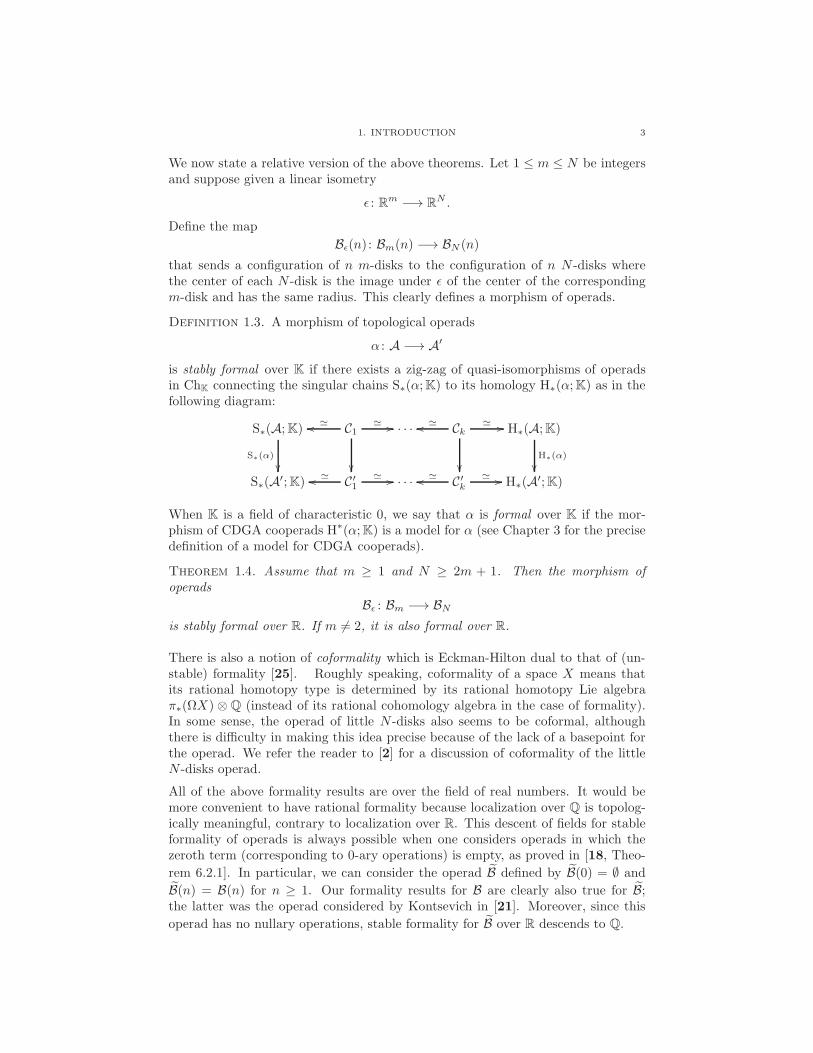
We now state a relative version of the above theorems. Let 1 ≤ m ≤ N be integersand suppose given a linear isometry

ǫ : Rm −→ RN .

Define the map

Bǫ(n) : Bm(n) −→ BN (n)

that sends a configuration of n m-disks to the configuration of n N -disks wherethe center of each N -disk is the image under ǫ of the center of the correspondingm-disk and has the same radius. This clearly defines a morphism of operads.

Definition 1.3. A morphism of topological operads

α : A −→ A′

is stably formal over K if there exists a zig-zag of quasi-isomorphisms of operadsin ChK connecting the singular chains S∗(α;K) to its homology H∗(α;K) as in thefollowing diagram:

S∗(A;K)

S∗(α)

C1≃oo ≃ //

· · · Ck≃oo ≃ //

H∗(A;K)

H∗(α)

S∗(A′;K) C′1

≃oo ≃ // · · · C′k≃oo ≃ // H∗(A′;K)

When K is a field of characteristic 0, we say that α is formal over K if the mor-phism of CDGA cooperads H∗(α;K) is a model for α (see Chapter 3 for the precisedefinition of a model for CDGA cooperads).

Theorem 1.4. Assume that m ≥ 1 and N ≥ 2m + 1. Then the morphism ofoperads

Bǫ : Bm −→ BNis stably formal over R. If m 6= 2, it is also formal over R.

There is also a notion of coformality which is Eckman-Hilton dual to that of (un-stable) formality [25]. Roughly speaking, coformality of a space X means thatits rational homotopy type is determined by its rational homotopy Lie algebraπ∗(ΩX) ⊗ Q (instead of its rational cohomology algebra in the case of formality).In some sense, the operad of little N -disks also seems to be coformal, althoughthere is difficulty in making this idea precise because of the lack of a basepoint forthe operad. We refer the reader to [2] for a discussion of coformality of the littleN -disks operad.

All of the above formality results are over the field of real numbers. It would bemore convenient to have rational formality because localization over Q is topolog-ically meaningful, contrary to localization over R. This descent of fields for stableformality of operads is always possible when one considers operads in which thezeroth term (corresponding to 0-ary operations) is empty, as proved in [18, Theo-

rem 6.2.1]. In particular, we can consider the operad B defined by B(0) = ∅ and

B(n) = B(n) for n ≥ 1. Our formality results for B are clearly also true for B;the latter was the operad considered by Kontsevich in [21]. Moreover, since this

operad has no nullary operations, stable formality for B over R descends to Q.

4 1. INTRODUCTION

For our applications to embedding spaces [3, 24], however, it is important to takethe usual little balls operad, B, which is only formal over R. In those applications,this weaker formality is sufficient essentially because the main results there areabout collapse of spectral sequences, and these collapse results do not depend onwhich field of characteristic 0 is used. The proof of descent of formality in [18,Section 6] does not generalize easily to the case with nullary operations because ofthe lack of minimal models when these degeneracy operations occur.

The formality of the operad B implies the formality overQ of each space B(n), in thesense that the CDGA APL(B(n)) is weakly equivalent to its cohomology algebra,H∗(B(n);Q). Paolo Salvatore has recently proved using a computer that, for n = 4and N = 2, the space B2(4) is not formal over the ring Z/2, i.e. its cohomologyalgebra, H∗(B2(4);Z/2), and its algebra of singular cochains, S∗(B2(4);Z/2), arenot quasi-isomorphic. We do not know whether the (non-symmetric) little disksoperad is stably formal over some field of positive characteristic.

As a final comment, the Tamarkin’s and Kontsevich’s proofs of formality for N = 2have been compared in [27] where it is proved that the weak equivalences obtainedin those two proofs are homotopic.

We end this introduction by explaining the general idea of Kontsevich’s proof offormality that we develop in this paper. The main ingredient is a combinatorialCDGA cooperad D = D(n)n≥0 of admissible diagrams and an explicit CDGAmap

(1.1) I : D(n) −→ ΩPA(C[n])

which we will call the Kontsevich configuration space integral . Here C[n] are com-pact manifolds homotopy equivalent to B(n), and ΩPA is a semi-algebraic analogof the deRham CDGA of differential forms ΩDR. A combinatorial argument willshow that the cooperad D is quasi-isomorphic to the cohomology of the little ballsoperad. We will also show that I is a quasi-isomorphism and, since I also respectsthe cooperad structures, the desired result will follow.

Let us elaborate on D(n) and I a bit further. We will work with the Fulton-MacPherson operad C[•] = C[n]n≥0 which is homotopy equivalent to the littleballs operad. The space C[n] is a compact manifold with corners obtained by addinga boundary to the open manifold Fn(R

N ), the space of configurations of n pointsin RN , that is,

Fn(RN ) := (z1, . . . , zn) ∈ (RN )n : zi 6= zj for i 6= j

(after normalizing by modding out by translations and positive dilations). Arnold[1] computed the cohomology algebra of Fn(R

2) = Fn(C) and in fact proved thatthese spaces are formal over C. His argument is as follows:

Consider the complex smooth differential one-forms

(1.2) ωij :=d(zj − zi)

zj − zi= d log(zj − zi) ∈ Ω1

DR(Fn(C);C)

which are cocycles and can easily be shown to be cohomologically independent for1 ≤ i < j ≤ n. A direct computation shows that these forms satisfy the 3-termrelation

(1.3) ωij ∧ ωjk + ωjk ∧ ωki + ωki ∧ ωij = 0.

1. INTRODUCTION 5

It is convenient to represent this relation by the diagram pictured in Figure 1.1.

+

ji1 k nj1 1 i ji k n k n

+

Figure 1.1. Diagrammatic description of the 3-term relation.

In this figure, the vertices on the line correspond to the labels of the points z1, . . . , znof a configuration and each edge (u, v) between two vertices represents a differentialform ωuv.

The subalgebra of ΩDR(Fn(C);C) generated by the ωij is

∧(ωij : 1 ≤ i < j ≤ n)

(ωij ∧ ωjk + ωjk ∧ ωki + ωki ∧ ωij).

This algebra has a trivial differential and it maps to the cohomology algebraH∗(Fn(C);C). A Serre spectral sequence argument shows that this map is ac-tually an isomorphism. In other words, the cohomology embeds in the deRhamalgebra of forms, and hence Fn(C) is formal.

Arnold’s argument for N = 2 can be generalized to all N as follows. Consider thedifferential forms ωij = θ∗ij(vol) where

θij : Fn(RN ) −→ SN−1

(z1, . . . , zn) 7−→ zj − zi‖zj − zi‖

,

and vol ∈ ΩN−1DR (SN−1) is the symmetric volume form on the sphere SN−1 that

integrates to 1. For N = 2, these are analogous to (1.2). It is well known by workof F. Cohen that these forms generate the cohomology algebra of Fn(R

N ) and thatthe 3-term relation holds in cohomology. However, the relation is not always trueat the level of forms. One only knows that, for each i, j, and k, there exists somedifferential form β such that

(1.4) dβ = ωij ∧ ωjk + ωjk ∧ ωki + ωki ∧ ωij .

The key idea now is to describe an algorithm which constructs in a natural way sucha cobounding form β. To explain this, suppose that n = 3 and (i, j, k) = (1, 2, 3).Consider the projection

(1.5) π : F4(RN ) −→ F3(R

N )

that forgets the fourth point of the configuration. It is a fibration with fiber

F = RN \ z1, z2, z3.

We will obtain β by integration along the fiber of π of some suitable differentialform α on F4(R

N ). To ensure convergence of the integral, we replace the spacesin the fibration (1.5) by their Fulton-MacPherson compactifications C[4] and C[3]so that the fiber becomes diffeomorphic to a closed disk in RN with three smallopen disks removed. We will denote this fiber by F . Intuitively, each of the threeinner boundary spheres of F corresponds to points z4 becoming infinitesimaly close

6 1. INTRODUCTION

to z1, z2, or z3, (which we denote by z4 ≃ zi), and the outer boundary sphere ofF corresponds to the point z4 going to infinity (which we denote by z4 ≃ ∞)).

Now consider the map

(1.6) θ := (θ14, θ24, θ34) : C[4] −→ SN−1 × SN−1 × SN−1.

The pullback form

θ∗(vol× vol× vol)

is a cocycle in Ω3N−3DR (C[4]) and is exactly

ω14 ∧ ω24 ∧ ω34.

Integration along the fiber of π is a linear map

π∗ =

F

: Ω3N−3DR (C[4]) −→ Ω2N−3

DR (C[3])

α 7−→

F

α.

The integration takes place along the variable z4 in the fiber F which corresponds tothe fourth component of a configuration z ∈ C[4]. The map π∗ satisfies a fiberwiseStokes formula

(1.7) d(

F

α) =

F

d(α) ±

∂F

α.

When α = ω14 ∧ω24 ∧ω34, the first term on the right side of (1.7) vanishes becauseα is a cocyle. We study its second term. One of the boundary components of Fcorresponds to z4 ≃ z1 ⊂ ∂F , and θ14 restricts to a diffeomorphism

θ14 : z4 ≃ z1∼=−→ SN−1.

We then have

z4≃z1

ω14∧ω24∧ω34 =

z4≃z1

ω14∧ω21∧ω31 =

ˆ

SN−1

vol

·ω21∧ω31 = ω21∧ω31.

Similarly the components corresponding to z4 ≃ z2 and z4 ≃ z2 give the two othersummands of the 3-term relation (1.3). Another argument shows that the integralalong the outer boundary corresponding to z4 ≃ ∞ vanishes. Thus

β :=

F

α

satisfies Equation (1.4) and is naturally defined.

This algorithm for constructing β can be encoded by a diagram Γ as pictured inFigure 1.2. In this diagram, vertices 1, 2, 3 (pictured on a line segment) are calledexternal and vertex 4 is called internal.

The three edges (1, 4), (2, 4), and (3, 4) correspond to the three components of themap θ from (1.6). To such a diagram we have associated the differential form

(1.8) I(Γ) :=

fiber

θ∗14(vol) ∧ θ∗24(vol) ∧ θ∗34(vol) = π∗(θ∗(×

3vol))

1. PLAN OF THE PAPER 7

4

1 2 3

Figure 1.2. The diagram Γ that cancels the 3-term relation from Figure 1.1.

where the points of the fiber are those labeled by internal vertices in the diagramΓ (that is, not on the horizontal line, which is z4 in this case).

We define the coboundary of such a diagram Γ by taking the sum over all possiblecontractions of an edge with not all endpoints on the line. In particular, for Γ asin Figure 1.2, its coboundary is exactly the diagrams of Figure 1.1 correspondingto the 3-term relation specialized to n = 3 and (i, j, k) = (1, 2, 3). Applying I,defined similarly as in (1.8), to the diagrams of Figure 1.1 gives the right hand sideof (1.4), which we have shown to be d(I(Γ)). In other words, I commutes with thedifferential in this example.

The vector space of all such “admissible” diagrams will be denoted by D and willbe endowed with the structure of a cooperad in CDGA. The generalization ofFormula (1.8) will define the Kontsevich configuration space integral I from (1.1).An algebraic computation will show that D(n), where n is the number of externalvertices (the ones drawn on the horizontal line segment), is quasi-isomorphic toH∗(C[n]), from which we will deduce that I in (1.1) is a quasi-isomorphism andhence that C[n] is formal. Since these quasi-isomorphisms respect the cooperadicstructure, this will prove the formality of the operad C[•] which is equivalent to thelittle disks operad.

There is one last technical issue. The operad structure on C[n] corresponds tothe inclusions of various faces of the boundary of C[n]. Therefore, in order for I tobe a map of cooperads, it is essential that the forms I(Γ) are well-defined on thisboundary. However, the projection

π : C[n+ l] −→ C[n]

is unfortunately not a smooth submersion on the boundary ∂ C[n] (see Exam-ple 5.9.1), and hence I(Γ) need not be a smooth form on this boundary. To fixthis problem we will replace ΩDR by the CDGA ΩPA of PA forms as defined in[23, Appendix]. These were studied in great detail in [19] and are reviewed inChapter 4.

1. Plan of the paper

For a faster run through this paper, the reader could, after reading the Introduction,jump directly to the beginning of Chapter 9 to get a better idea of the constructionof the quasi-isomorphism of operads

I : D(•) −→ ΩPA(C[•])

8 1. INTRODUCTION

which is central to our proofs. Along the way, a quick look at Sections 5.1 and6.1–6.2 will supply a better sense of the Fulton-MacPherson operad C[•] and theCDGA cooperad of admissible diagrams D(•), respectively.The plan of the paper is as follows (see also the Table of Contents at the beginningof the paper).

• In Chapter 2 we fix some notation, and in particular establish some terminol-ogy relating to linear orders and weak ordered partitions which will be useful indescribing the operad structure maps.

• In Chapter 3 we define in detail what we mean by formality for operads. This isnot as straighforward as one might wish because the Sullivan-deRham functor APL

(or its semi-algebraic analog ΩPA) does not turn operads into genuine cooperadsof CDGAs. Our definition, however, is practical enough for applications.

• In Chapter 4 we review the functor ΩPA of PA forms. This is the analog forsemi-algebraic spaces of the deRham functor ΩDR of differential forms for smoothmanifolds. We review the main results we will need from this theory, such asthe notion of semi-algebraic chains C∗(X) on a semi-algebraic set X , which areweakly equivalent to singular chains; the fact that ΩPA encodes (monoidaly) thereal homotopy type of compact semi-algebraic sets; and the important notion ofintegration along the fiber, or pushforward, of a “minimal” PA form along a semi-algebraic bundle.

• In Chapter 5 we define and study in detail the Fulton-MacPherson operad C[•]and prove the results about this operad that are necessary for establishing certainproperties of the Kontsevich configuration space integral. We also review the factthat the Fulton-MacPherson operad is equivalent to the little balls operad.

• In Chapter 6 we construct the combinatorial CDGA D(n) of admissible diagrams

(on n external vertices), built from a larger companion CDGA D(n) of diagrams.The CDGA D(n) will later be shown to be quasi-isomorphic to both ΩPA(C[n])and its cohomology.

• In Chapter 7 we endow first D and then D with the structure of a cooperad.The cooperad structure is obtained by considering condensations , which will havealready appeared in the study of the Fulton-MacPherson operad in Chapter 5.

• In Chapter 8, we prove that the cooperadD is quasi-isomorphic to the cohomologyof the Fulton-MacPherson operad.

• In Chapter 9 we construct the Kontsevich configuration space integrals, whichare CDGA maps

I : D(n) −→ ΩPA(C[n]) and I : D(n) −→ ΩPA(C[n]).

We prove that they are (almost) morphisms of cooperads. The arguments use manyproperties of the Fulton-MacPherson operad developed in Chapter 5.

• In Chapter 10 we collect the results of the previous two chapters to deduce ourmain formality results. In particular, we prove that I is a quasi-isomorphism.

• Lastly, for the convenience of the reader we have included an index of notationin the Appendix.

CHAPTER 2

Notation, linear orders, weak partitions, and

operads

In this chapter we fix some notation, most of which is standard. We also review thenotion of linear orders and introduce the notion of a weak ordered partition whichis useful in describing the operad structure maps.

2.1. Notation

K will be a commutative ring with unit, often R.

An integer N ≥ 1 (which gives the ambient dimension) will be fixed.

For a set A we denote by |A| its cardinality. We denote by Perm(A) the group ofpermutations of A. For a nonnegative integer n, we set n = 1, . . . , n. We willsometimes identify n and the set n. The set of all functions from a set X to a setY is denoted by Y X .

When f : X → Y is a map and A ⊂ X , we denote the restriction of f to A by f |A.We denote the one-point space by ∗.We use the notation x := def to state that the left hand side is defined by the righthand side.

An extended index of notation is in the Appendix.

2.2. Linear orders

Definition 2.2.1. A linearly ordered (or a totally ordered) set is a pair (L,≤)where L is a set and ≤ is a reflexive, transitive, and antisymmetric relation on Lsuch for any x, y ∈ L we have x ≤ y or y ≤ x. We write x < y when x ≤ y andx 6= y.

Given two disjoint linearly ordered sets (L1,≤1) and (L2,≤2) their ordered sum isthe linearly ordered set L1 < L2 := (L1 ∪ L2,≤) such that the restriction of ≤ toLi is the given order ≤i and such that x1 ≤ x2 when x1 ∈ L1 and x2 ∈ L2.

More generally if Lpp∈P is a family of linearly ordered sets indexed by a linearlyordered set P , its ordered sum

<p∈P

Lp

is the disjoint union ∐p∈PLp equipped with a linear order ≤ whose restriction toeach Lp is the given order on that set and such that x < y when x ∈ Lp and y ∈ Lq

with p < q in P .

9

10 2. NOTATION, LINEAR ORDERS, WEAK PARTITIONS, AND OPERADS

It is clear that the ordered sum < is associative but not commutative.

We define the position function on a linearly ordered finite set (L,≤) as the uniqueorder-preserving isomorphism

pos : L −→ 1, . . . , |L|.We write pos(x : L) for pos(x) when we want to emphasize the underlying orderedset L.

2.3. Weak ordered partitions

The following terminology will be useful in the description of operad structures inthe next section.

Definition 2.3.1. A weak partition of a finite set A is a map ν : A→ P , where Pis a finite set. The preimages ν−1(p), for p ∈ P , are the elements of the partition.Since we do not ask ν to be surjective, some of the elements ν−1(p) can be empty,and hence the adjective weak. The weak partition is degenerate if ν is not surjective,and non-degenerate otherwise. We will simply say partition for a non-degenerateweak partition. The (weak) partition ν is ordered if its codomain P is equippedwith a linear order. The undiscrete partition is the partition ν : A → 1 whoseonly element is A.

2.4. Operads and cooperads

Here we review the definition of operads that we will use. Let (C,⊗,1) be a sym-metric monoidal category. Let IsoFin be the category whose objects are finite sets(including the empty set) and whose morphisms are bijections between them. Thiscategory is equivalent to the category with one object for each integer n ≥ 0 alongwith the symmetric group Σn = Perm(n) as its set of automorphisms, and no othermorphisms. A symmetric sequence in C is a functor

O : IsoFin −→ C.Thus a symmetric sequence in C is determined by a sequence (O(n))n≥0 of objectsof C together with an action of Σn on O(n).An operad O is a symmetric sequence together with a unit map

u : 1 −→ O(1)and, for each ordered weak partition ν : A→ P , natural operad structure maps

(2.1) Θν : O(P ) ⊗ ⊗p∈PO(ν−1(p)) −→ O(A)

satisfying the usual associativity, unital, and equivariance conditions. Here themonoidal product ⊗

p∈Pis taken of course in the linear order of P .

A cooperad is an operad in the opposite category.

Our operads have an objectO(0) = O(∅) in arity 0. If we were working with operadswithout a nullary term, then we would only need non-degenerate partitions ν.

When investigating (co)operads, we will often fix the following setting:

2.4. OPERADS AND COOPERADS 11

Setting 2.4.1. Fix an ordered weak partition ν : A→ P , with A and P finite, andP linearly ordered. We assume that 0 6∈ P and set

(2.2) P ∗ := 0< P

where < is the ordered sum defined in Section 2.2. Set Ap = ν−1(p) for p ∈ P , andA0 = P .

Under this setting the structure maps (2.1) become

Θν : ⊗p∈P∗

O(Ap) −→ O(A).

CHAPTER 3

CDGA models for operads

In this chapter we give precise meaning to the notion of a CDGA model for a topo-logical operad or for a morphism of topological operads. Our definition, althoughnot difficult, is perhaps not so elegant, but it suffices for the applications we have inmind. At the end of the chapter we sketch an alternative, more concise definition.

Recall that Sullivan [31] (see [8] or [12] for a complete development of the theory)constructed a contravariant functor of piecewise polynomial forms over a field K ofcharacteristic 0,

APL(−;K) : Top −→ CDGA

which mimics the deRham differential algebra of smooth differential forms on a man-ifold. Here CDGA is the category of commutative differential graded K−algebras(or CDGA for short) which are non-negatively graded. Sometimes we will also con-sider Z-graded CDGAs which can be non trivial in negative degree, but those arenot the objects of the category CDGA. A CDGA (A, d) is a CDGA model (over K)for a space X if the CDGAs (A, d) and APL(X ;K) are weakly equivalent, by whichwe mean that there exists a chain of quasi-isomorphisms of CDGAs connectingthem:

(A, d)≃←− · · · ≃−→ APL(X ;K).

The main feature of the theory is that when X is a simply-connected topologi-cal space with finite Betti numbers and K = Q, then any CDGA model for Xdetermines the rational homotopy type of X . Moreover, many rational homotopyinvariants, like the rational cohomology algebra H∗(X ;Q) or the rational homotopyLie algebra π∗(ΩX)⊗ Q can easily be recovered from the model (A, d). For fieldsK other than the rationals, we have

APL(−;K) = APL(−;Q)⊗Q K,

and by extension we say that the quasi-isomorphism type of APL(X ;K) determinesthe K-homotopy type of X . We just write APL(X) when the field K is understood.

Also, if f : X → Y is a map of spaces, we say that a CDGA morphism

φ : (B, dB) −→ (A, dA)

is a CDGA model for f if there exists a zig-zag of weak equivalences connecting φand APL(f ;K), that is, if there exists a commutative diagram of CDGAs

(B, dB)

φ

•≃oo ≃ //

· · · •≃oo ≃ //

APL(Y ;K)

APL(f ;K)

(A, dA) •≃oo ≃ // · · · •≃oo ≃ // APL(X ;K)

13

14 3. CDGA MODELS FOR OPERADS

in which the horizontal arrows are quasi-isomorphisms.

We would like to define a similar notion of a CDGA model for a topological operadO. A naive definition would be that such a model is a cooperad A of CDGAsthat is connected by weak equivalences of CDGA cooperads to APL(O). However,there is a problem with this definition because the contravariant functor APL is notcomonoidal as there is no suitable natural map

(3.1) APL(X × Y ) −→ APL(X)⊗APL(Y ).

Therefore it seems that there is no cooperad structure on APL(O) naturally inducedfrom the operad structure on O. On the other hand, APL is monoidal through theKunneth quasi-isomorphism

(3.2) κ : APL(X)⊗APL(Y )≃−→ APL(X × Y ).

This morphism becomes an isomorphism in the homotopy category, and its inverseshould correspond to the homotopy class of the missing map (3.1). We would thuslike to say that APL(O) is a cooperad “up to homotopy”. However, this sort of“up to homotopy” structure needs to be handled with more care than is necessaryfor our purpose, and so we will not pursue this in detail here and will just give anindication of such a notion at the end of the chapter. Instead we will propose inDefinition 3.1 an ad hoc definition of a CDGA model for an operad.

There is a second difficulty which we will have do deal with and which comesfrom the proof of the formality itself. Namely, in Kontsevich’s proof of the weakequivalence between the (up to homotopy) cooperad APL(B) and its cohomology,a functor ΩPA (to be reviewed in Chapter 4) is used. This functor is weaklyequivalent to APL(−;R) but is defined only after restriction to a subcategory of Top,namely the category of compact semi-algebraic sets. This is analogous to the factthat the deRham CDGA of smooth differential forms ΩDR is weakly equivalent toAPL(−;R) after restriction to the subcategory of smooth manifolds. Consequently,our modeling functors will sometimes be defined on some subcategory u : T → Top.

To finally define our notion of a CDGA model for an operad, we will need a fewdefinitions.

Two cooperads of CDGAs, A and A′, are weakly equivalent if they are connectedby a chain of quasi-isomorphism of CDGA cooperads,

A ≃←− · · · ≃−→ A′.

Let (T ,×,1) be a symmetric monoidal category and let

u : T −→ Top

be a symmetric strongly monoidal covariant functor, where by strongly we meanthat the natural map

(3.3) u(X)× u(Y )∼=−→ u(X × Y )

is an isomorphism and u(1) = ∗ is the one-point space.

For us, a contravariant functor

Ω: T −→ CDGA

3. CDGA MODELS FOR OPERADS 15

is symmetric monoidal if it is equipped with a natural map

(3.4) κ : Ω(X)⊗ Ω(Y ) −→ Ω(X × Y )

satisfying the usual axioms and such that Ω(1) = K. In particular APL u issymmetric monoidal.

A natural monoidal quasi-isomorphism between two such contravariant symmetricmonoidal functors Ω and Ω′ is a natural transformation

θ : Ω −→ Ω′

that induces an isomorphism in homology and that commutes with the monoidalstructure maps. Two symmetric monoidal contravariant functors are weakly equiv-alent if they are connected by a chain of natural monoidal quasi-isomorphisms. If Ωis weakly equivalent to APLu then the morphism κ of (3.4) is a quasi-isomorphismbecause the corresponding one for APL in (3.2) is as well and because of the iso-morphism (3.3).

Our definition of CDGA models for cooperads is then

Definition 3.1. A CDGA cooperad A is a CDGA model for a topological operadO if there exist

• a CDGA cooperad A′ weakly equivalent to A;• a symmetric monoidal category (T ,×,1);• a symmetric strongly monoidal covariant functor u : T → Top;• an operad O′ in T such that u(O′) is weakly equivalent to O;• a symmetric monoidal contravariant functor Ω weakly equivalent to APL u;• for each n ≥ 0 a Σn-equivariant quasi-isomorphism

Jn : A′(n)≃−→ Ω(O′(n))

such that, for each k ≥ 0 and n1, . . . , nk ≥ 0 with n = n1 + · · ·+ nk, thefollowing diagram commutes:

A′(n)Jn

≃//

Ψ

Ω(O′(n))

Ω(Φ)

Ω(O′(k)×O′(n1)× · · · × O′(nk))

A′(k)⊗A′(n1)⊗ . . .A′(nk)≃

Jk⊗Jn1⊗···⊗Jnk

// Ω(O′(k))⊗ Ω(O′(n1))⊗ · · · ⊗ Ω(O′(nk)).

κ≃

OO

Here Ψ and Φ are the (co)operad structure maps onA′ andO′ respectively,and the composition

A′(1)J1−→ Ω(O′(1))

Ω(η)−→ Ω(1) ∼= K

is required to be the counit of A′, where η is the unit of O′.

16 3. CDGA MODELS FOR OPERADS

If κ was an isomorphism, then κ−1 Ω(Φ) would define a cooperad structure onΩ(O′) and the above diagram would simply mean that the cooperads A′ and Ω(O′)are weakly equivalent.

The main examples of the above that we will consider are:

• the category T = CompactSemiAlg of compact semi-algebraic sets (Chap-ter 4);• the forgetful functor u : CompactSemiAlg→ Top;• the functor Ω = ΩPA of semi-algebraic forms (Chapter 4);• the topological operad of little balls O = BN ;• the Fulton-MacPherson semi-algebraic operad O′ = C[•] (Chapter 5), and• its cohomology A = H∗(C[•]);• the cooperad of admissible diagrams A′ = D (Chapters 6-7); and• the Kontsevich configuration space integral Jn = I: D(n) → ΩPA(C[n])(Chapter 9).

We will let the reader generalize Definition 3.1 in an obvious way to say when amorphism of CDGA cooperads

φ : A1 −→ A2

is a CDGA model for a morphism of topological operads

f : O2 −→ O1.

Definition 3.2. A topological operad is formal over K if the induced cohomologyalgebra cooperad is a CDGA model for this operad over K.

A morphism of topological operads is formal if the induced morphism in cohomologyis a CDGA model for this operad morphism.

This definition, albeit perhaps a bit ad hoc, is good enough for the applications wehave in mind. A more elegant definition would have to use a precise notion of a(co)operad up to homotopy as follows.

Recall, for example from [16, §1.2], that an operad can be seen as a functor on thecategory of trees. More precisely let Tree be the category whose objects are rootedplanar trees and morphisms compositions of contractions of non-terminal edges.Given trees S, T1, . . . , Tk where S has k leaves and each Ti has ni leaves, one canbuild a new tree S(T1, . . . , Tk) with n1+ · · ·+nk leaves by grafting the root of eachtree Ti to the corresponding leaf of S. For n ≥ 0 we denote by 〈n〉 the tree with nleaves and no internal vertex, that is a tree which is indecomposable with respectto the grafting operation. Then an operad O in a symmetric monoidal category Ccan be seen as a functor

O : Tree −→ Cwhere O(〈n〉) = O(n), for n ≥ 0. In order for a functor O to define an operad oneasks for isomorphisms

α(S,T1,...,Tk) : O(S(T1, . . . , Tk))∼=−→ O(S) ⊗⊗k

i=1O(Ti)

satisfying obvious associativity, unital, and equivariance relations.

There is a morphism in Tree given by

〈k〉(〈n1〉, . . . , 〈nk〉) −→ 〈n1 + · · ·+ nk〉

3. CDGA MODELS FOR OPERADS 17

and its image under the functor O composed with the inverse of the isomorphismα gives the structure maps of the operad.

An operad up to homotopy is an analogous functor O except that one only asksα(S,T1,...,Tk) to be a weak equivalence instead of an isomorphism. Similarly we candefine cooperads up to homotopy.

If O is a topological operad, then APL(O) naturally becomes a cooperad up tohomotopy in this sense, with the weak equivalences α constructed from the Kun-neth quasi-isomorphism (3.2). There is also an obvious notion of morphisms of(co)operads up to homotopy and of weak equivalences. One could check that ifa CDGA cooperad A is a CDGA model for a topological operad O in the senseof Definition 3.1, then A and APL(O) are also weakly equivalent as cooperads upto homotopy. This therefore might give a better definition of an operad model,but it is possible that some further “∞-version” would be necessary for obtainingsomething useful.

CHAPTER 4

Real homotopy theory of semi-algebraic sets

In this chapter we give a brief review of Kontsevich and Soibelman’s theory of semi-algebraic differential forms which is outlined in [23, §8]. In particular we discuss thefunctor ΩPA which is analogous to the deRham functor ΩDR for smooth manifolds.That functor and the way it encodes real homotopy theory of semi-algebraic setswas developed in full detail by the authors jointly with Robert Hardt and VictorTurchin in [19].

Definition 4.1 ([6]). A semi-algebraic set is a subset of Rp that is obtained byfinite unions, finite intersections, and complements of subsets defined by polynomialequations and inequalities. A semi-algebraic map is a continuous map betweensemi-algebraic sets whose graph is a semi-algebraic set.

We will consider the categories SemiAlg (and CompactSemiAlg) of (compact) semi-algebraic sets. Endowed with the cartesian product, this category becomes sym-metric monoidal and the obvious forgetful functor

u : SemiAlg −→ Top

is strongly symmetric monoidal because of the natural homeomorphism

u(X)× u(Y )∼=−→ u(X × Y ).

We have for a semi-algebraic set X a functorial chain complex of semi-algebraicchains C∗(X) [19, Definition 3.1], which is weakly equivalent to singular chains.A typical element of Ck(X) is represented by a semi-algebraic map g : M → Xfrom a semi-algebraic compact oriented manifold M of dimension k. This elementis denoted by g∗(JMK) ∈ Ck(X). In particular, taking g = idM ,

(4.1) JMK ∈ Ck(M)

represents a canonically defined fundamental class of the manifold M at the levelof semi-algebraic chains. Also, a semi-algebraic map f : X → Y induces a chainmap

(4.2) f∗ : C∗(X) −→ C∗(Y ).

We in addition have a contravariant functor of minimal forms [19, Section 5.2]

(4.3) Ωmin : SemiAlg −→ CDGA .

By definition, a minimal form of degree k on X is represented by a linear combi-nation of

µ = f0 · df1 ∧ · · · ∧ dfk

wheref0, f1, . . . , fk : X −→ R

19

20 4. REAL HOMOTOPY THEORY OF SEMI-ALGEBRAIC SETS

are semi-algebraic maps. Even though the fi’s may not be everywhere smooth, wecan define a differential dµ which is again a minimal form. Also for a compact semi-algebraic oriented manifoldM of dimension k and a semi-algebraic map g : M → X ,we can evaluate the form µ on g∗(JMK) ∈ Ck(X) by the formula

(4.4) 〈µ , g∗JMK〉 :=ˆ

M

g∗(f0 · df1 ∧ · · · ∧ dfk).

The convergence of the integral on the right is a consequence of the semi-algebraicityof M . Indeed that integral is the same as

(4.5)

ˆ

f∗(g∗(M))

x0 · dx1 ∧ · · · ∧ dxk

where f∗(g∗(M)) is the image of M in Rk+1 (counted with multiplities) under thecomposition of g and f := (f0, f1, . . . , fk). Thus f∗(g∗(M)) is a compact semialgebraic-set of dimension ≤ k, which implies that its k-volume is finite (this wouldnot be true for non semi-algebraic compact sets.) Hence the integral in Equa-tion (4.5) converges. See [19, Theorem 2.4 and beginning of Section 3] for moredetails.

In this paper, the only minimal forms that we will use are the standard volumeform on the sphere and its pullbacks along semi-algebraic maps.

The CDGA of minimal forms embeds in that of PA forms [19, Section 5.4] (“PA”stands for “piecewise algebraic”)

(4.6) ΩPA : SemiAlg −→ CDGA .

Roughly speaking, PA forms are obtained by integration along the fiber of min-imal forms along oriented semi-algebraic bundles, which are recalled below. Theimportant feature is the following

Theorem 4.2 ([19, Theorem 7.1]). When restricted to the category of compactsemi-algebraic sets, the contravariant symmetric monoidal functors ΩPA andAPL(u(−);R) are weakly equivalent.

Another important feature of minimal and PA forms is that classical integrationalong the fiber for smooth forms can be extended to the semi-algebraic framework.To explain, we have from [19, Section 8] the notion of a semi-algebraic bundle, orSA bundle for short, which is the obvious generalization of the usual definition ofa locally trivial bundle.

An SA bundleπ : E −→ B

is oriented if its fibers are compact oriented semi-algebraic manifolds, with orien-tation which is locally constant in an obvious sense. For each b ∈ B we then havethe fundamental class of the fiber over b,

(4.7) Jπ−1(b)K ∈ Ck(π−1(b)),

where k is the dimension of the fiber.

Given an oriented SA bundle π : E → B whose fibers are compact SA manifolds,there exists a subbundle

(4.8) π∂ : E∂ → B

4. REAL HOMOTOPY THEORY OF SEMI-ALGEBRAIC SETS 21

whose fibers are the boundaries of the fibers of π. This subbundle is called thefiberwise boundary of π (see [19, Definition 8.1]). An example is the map

proj1 : E := [0, 1]× [0, 1]→ [0, 1]

which projects onto the first factor. In this case the fiberwise boundary is E∂ =[0, 1]× 0, 1, but this is not the boundary of E.

For an oriented SA bundle with k-dimensional fiber, there is a linear map of degree−k [19, Definition 8.3],

(4.9) π∗ : Ω∗+kmin (E) −→ Ω∗

PA(B),

which correponds to integration along the fiber, also called pushforward. In somesense PA forms are obtained as (generalized) pushforwards of minimal forms [19,Definition 5.20]. Properties of the pushforward that we will need here are collectedin [19, Section 8.2]. They are analogous to the standard properties of integration ofsmooth differential forms along the compact fiber of a smooth bundle. In particularone has a fiberwise Stokes formula which we will need later.

CHAPTER 5

The Fulton-MacPherson operad

Fix N ≥ 1. In this chapter we review the Fulton-MacPherson operad

C[•] = C[n]n≥0

which is weakly equivalent to the little N -disks operad. As a space, each C[n] is acompactification of the space C(n) of normalized ordered configurations of n pointsin RN . It is a compact semi-algebraic manifold with boundary, and so its real ho-motopy type is encoded by the semi-algebraic analog of deRham theory, ΩPA(C[n]).The operad structure maps correspond essentially to inclusions of various faces ofthe boundary ∂ C[n].

We will also in this chapter study canonical projections

π : C[n+ l] −→ C[n]

given by forgetting some points of the configuration and will prove that they areSA bundles with compact manifolds as fibers. This fact will be used in Section 9.1to construct the Kontsevich configuration space integral I : D(n) → ΩPA(C[n]) of(1.1) via integration along the fiber of π. We will also study the interaction of thesecanonical projections with the operad structure in order to later prove that I is amap of cooperads.

The plan of this chapter is the following:

5.1: We define the compactification C[n], compute its dimension, and charac-terize its boundary.

5.2: We describe the operad structure on C[n]n≥0 and recall that this operadis equivalent to the operad of little balls.

5.3: We study the canonical projection π : C[n + l] → C[n] and state that itdefines a bundle whose fibers are oriented compact manifolds.

5.4: We decompose the boundary ∂ C[n] into faces which are images of the i(“circle-i”) operad maps.

5.5: We construct singular configuration spaces which are variations of spacesC[n] and will be needed for some technical points.

5.6: In this (long) section, we investigate the pullback of a canonical projec-tion along an operad structure map. This will be needed for provingthat the Kontsevich configuration space integral respects the (co)operadicstructures. We introduce at the beginning of this section the notion of acondensation which will also be needed for the definition of the cooperadstructure on the space of diagrams in Chapter 7.

5.7: We describe a decomposition of the fiberwise boundary of the total spaceC[n + l] of a canonical projection. This will be used in proving thatKontsevich’s configuration space integral is a chain map.

23

24 5. THE FULTON-MACPHERSON OPERAD

5.8: We fix an orientation of C[n]; this will be important when we integrateforms over this manifold.

5.9: We prove Theorem 5.3.2, stated in Section 5.3, which asserts that thecanonical projections are oriented SA bundles. This section also containsan example showing that the canonical projections are not smooth bun-dles.

On a first pass of this chapter, the reader may just concentrate on Sections 5.1-5.4to acquire a good sense of the Fulton-McPherson operad. The last five sections aremore technical and are needed only for the details of the proof of certain propertiesof the Kontsevich configuration space integral in Chapter 9. However, the readershould still look at Definition 5.6.1 of a condensation in Section 5.6, as this will beneeded in Chapter 7 to define the cooperadic structure on the spaces of diagrams

D(n).

5.1. Compactification of configuration spaces in RN

We first recall the Fulton-MacPherson compactification C[n] of the configurationspace C(n) of n points in RN . This compactification (or at least some variation ofit) was defined in [13], with the operad structure given in [15], and alternativelyby Kontsevich in [21, Definition 12] and [22, Section 5.1]. We follow Kontsevich’sapproach, which was corrected by Gaiffi in [14, Section 6.2] and developed in detailby Sinha in [28] (the equivalence of the Kontsevich and the Fulton-MacPhersondefinitions follows from Sinha’s work as well).

Let A be a finite set of cardinality n which will serve as a set of labels for the pointsof the configurations. Consider the space

(5.1) Inj(A,RN ) := x : A → RNof all injective maps from A to RN . An element x ∈ Inj(A,RN ) is an (ordered)configuration (x(a))a∈A of n distinct points in RN . This space is topologized as asubspace of the product (RN )A =

∏a∈A RN .

The space Inj(A,RN ) is a smooth open manifold of dimension N · |A|. The group oforientation-preserving similarities RN⋊R+

0 acts by translation and positive dilationon RN , and hence diagonally on Inj(A,RN ). We denote its orbit space by

(5.2) C(A) := Inj(A,RN )/(RN ⋊R+0 ).

(This space is denoted by Cn(RN ) in [28, Definition 3.9].)

When |A| ≥ 2 the action is free and smooth and hence C(A) is a manifold ofdimension

dimC(A) = N · |A| −N − 1,

and when |A| ≤ 1 then C(A) is a one-point space because the action is transitive.

Define the barycenter of a map x : A→ RN as the point

(5.3) barycenter(x) = barycenter(x(a) : a ∈ A) :=1

|A|∑

a∈A

x(a)

and its radius as the real number

(5.4) radius(x) = radius(x(a) : a ∈ A) := max(‖x(a) − barycenter(x)‖ : a ∈ A).

5.1. COMPACTIFICATION OF CONFIGURATION SPACES IN RN 25

When |A| ≥ 2, C(A) is homeomorphic to the space of normalized configurations

(5.5) Inj10(A,RN ) :=

x ∈ Inj(A,RN ) : barycenter(x) = 0 and radius(x) = 1

.

We will use C(A) and Inj10(A,RN ) interchangeably. Most of the time in this paper,

a configuration will be denoted by x or y (maybe with some decoration) and, whenseen as an element of Inj10(A,R

N ), its components will be points x(a) for a anelement of the set of labels of the components, A.

Denote by SN−1 the unit sphere in RN . Given two distinct elements a, b ∈ A,consider the map

θa,b : C(A) −→ SN−1(5.6)

x 7−→ x(b)− x(a)

‖x(b)− x(a)‖which gives the direction between two points of the configuration.

For three distinct elements a, b, c ∈ A, also define

δa,b,c : C(A) −→ [0,+∞](5.7)

x 7−→ ‖x(a)− x(b)‖‖x(a)− x(c)‖

which gives the relative distance of 3 points of a configuration.

Set

A2 = (a, b) ∈ A×A : a 6= bA3 = (a, b, c) ∈ A×A×A : a 6= b 6= c 6= a

and consider the map

ι : C(A) −→ (SN−1)A2 × [0,+∞]A

3

x 7−→((θa,b(x))(a,b)∈A2 , (δa,b,c(x))(a,b,c)∈A3

).

Up to translation and dilation, any configuration x : A → RN can be recovered fromthe directions θa,b(x) and relative distances δa,b,c(x). Hence ι is a homeomorphismonto its image [28, Lemma 3.18] and we will identify C(A) with ι(C(A)).

Definition 5.1.1. The Fulton-MacPherson compactification C[A] of C(A) is thetopological closure of the image of ι, that is,

C[A] := ι(C(A)).

Intuitively, one should think of x ∈ C[A] as a “virtual” configuration in whichsome points are possibly infinitesimally close to each other in such a way that thedirection between any two points and the relative distance between three points isalways well-defined. These directions and relative distances are given by the mapsθa,b and δa,b,c, which obviously extend to C[A]. Moreover an element x ∈ C[A] iscompletely characterized by the values θa,b(x) ∈ SN−1 and δa,b,c(x) ∈ [0,+∞], fordistinct a, b, c ∈ A. By abuse of terminology an element x ∈ C[A] will be called aconfiguration and we will talk informally of its components x(a) ∈ RN , for a ∈ A.


The following notation will be useful: For a, b, c distinct in A and x ∈ C[A], whenδa,b,c(x) = 0 we write

(5.8) x(a) ≃ x(b) relx(c).

This happens exactly when the points x(a) and x(b) are infinitesimaly close toeach other in comparison to their distance to x(c). Pictorial interpretations of thissituation are given below in Example 5.2.1. In particular Figure 5.2 represents aconfiguration x ∈ C[6] with N = 2.

The space C(A) ⊂ (RN )A and the map ι are clearly semi-algebraic, therefore sois the closure C[A]. Moreover, by [7] or [28], C[A] is a compact manifold withcorners. It is easy to see that the atlases given in those papers are semi-algebraic,and hence C[A] is a compact semi-algebraic manifold with boundary (charts aregiven in Lemma 5.9.3).

In conclusion, we have

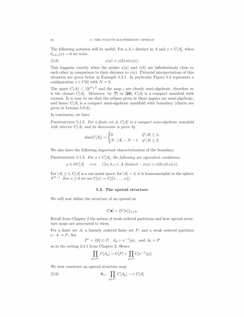
Proposition 5.1.2. For a finite set A, C[A] is a compact semi-algebraic manifoldwith interior C(A) and its dimension is given by

dim(C[A]) =

0 if |A| ≤ 1;

N · |A| −N − 1 if |A| ≥ 2.

We also have the following important characterization of the boundary

Proposition 5.1.3. For x ∈ C[A], the following are equivalent conditions:

x ∈ ∂ C[A] ⇐⇒ (∃ a, b, c ∈ A distinct : x(a) ≃ x(b) relx(c)).

For |A| ≤ 1, C[A] is a one-point space; for |A| = 2, it is homeomorphic to the sphereSN−1. For n ≥ 0 we set C[n] := C[1, . . . , n].

5.2. The operad structure

We will now define the structure of an operad on

C[•] = C[n]n≥0.

Recall from Chapter 2 the notion of weak ordered partitions and how operad struc-ture maps are associated to them.

Fix a finite set A, a linearly ordered finite set P , and a weak ordered partitionν : A→ P . Set

P ∗ = 0< P, Ap = ν−1(p), and A0 = P

as in the setting 2.4.1 from Chapter 2. Hence∏

p∈P∗

C[Ap] = C[P ]×∏

p∈P

C[ν−1(p)].

We now construct an operad structure map

(5.9) Φν :∏

p∈P∗

C[Ap] −→ C[A]

5.2. THE OPERAD STRUCTURE 27

as follows. Intuitively the configuration x = Φν((xp)p∈P∗) is obtained by replacing,for each p ∈ P , the p-th component x0(p) of the configuration x0 ∈ C[P ] by theconfiguration xp ∈ C[Ap] made infinitesimal. To illustrate, we first give an example.

Example 5.2.1. Consider P = α, β, γ, δ (with the linear order α < β < γ < δ),A = 1, 2, 3, 4, 5, 6, and let ν : A→ P be given by

ν(a) =

α, for a = 1, 2;

β, for a = 3, 4, 5;

δ, for a = 6.

Consider

x0 ∈ C[P ] ∼= C[4];

xα ∈ C[1, 2] ∼= C[2];

xβ ∈ C[3, 4, 5] ∼= C[3];

xγ ∈ C[∅] ∼= C[0] = ∗;xδ ∈ C[6] ∼= C[1] = ∗

and suppose that these configurations are for example as in Figure 5.1 (withN = 2).

6

βx0 =γ

δα

xα =

2

1 xβ =

5

4

3

xγ = xδ =

Figure 5.1

This kind of pictorial representation of compactified configuration spaces first ap-peared in [28]. The plane represents RN and the “funnels” represent infinitesimalconfigurations. Thus for example, in the picture of x0, points labeled by α and δare infinitesimally close to each other from the point of view of β and γ. In notationof relation (5.8), x0(α) ≃ x0(δ) relx0(β) and x0(α) ≃ x0(δ) relx0(γ). Similarly inthe picture of x in Figure 5.2 below, points (labeled by) 4, 3, and 5 are infinites-imally close to each other from the point of view of 6, 1, and 2, but 3 and 5 areinfinitesimally close to each other from the point of view of 4, as are 1 and 2 fromthe point of view of 6.

Then the configuration x = Ψν(x0, xα, xβ , xγ , xδ) can be represented as in Figure5.2.

More precisely, x = Φν((xp)p∈P∗) ∈ C[A] is characterized by, for distinct a, b, c ∈ A,

θa,b(x) =

θa,b(xp), if a, b ∈ Ap for some p ∈ P, that is ν(a) = ν(b) = p;

θν(a),ν(b)(x0), if ν(a) 6= ν(b),


6

1

x =

4

3 52

Figure 5.2

and

δa,b,c(x) =

δa,b,c(xp), if a, b, c ∈ Ap for some p ∈ P ;

δν(a),ν(b),ν(c)(x0), if ν(a), ν(b), and ν(c) are all distinct;

0, if ν(a) = ν(b) 6= ν(c);

1, if ν(a) 6= ν(b) = ν(c);

+∞, if ν(a) = ν(c) 6= ν(b).

There is an obvious action of the group Perm(A) of permutations of the set A onC[A], and in particular of the symmetric group Σn on C[n]. We define the unit inC[1] as its unique point (or more precisely the unique map u : ∗ → C[1]).

The following is straightforward to check (see for example [29, Section 4]).

Proposition 5.2.2. The above data endows C[•] = C[n]n≥0 with the structureof an operad of compact semi-algebraic sets.

The relevance of the Fulton-MacPherson operad for us is that it is weakly equivalentto the little balls operad, as proved by P. Salvatore:

Proposition 5.2.3. [26, Proposition 4.9] The Fulton-MacPherson operad C[•] ofconfigurations in RN and the little N -disks operad B are weakly equivalent as topo-logical operads.

For the sake of keeping this paper as self-contained as possible, we summarizeSalvatore’s proof here.

Summary of proof of Proposition 5.2.3. Recall the W construction ofBoardman-Vogt [5] which associates to a topological operad O(•) another operadWO consisting of planar rooted trees τ whose internal edges have length between0 and 1 and whose internal vertices of valence i+1 are decorated by an element ofO(i). The operad WO is a cofibrant replacement of O. The main idea of the proofis then to construct a map R : WB → C[•] that sends a decorated tree τ to the con-figuration of the centers of the configuration of balls obtained by multicompositionof all the configurations of balls associated to the vertices of τ (after rescaling theconfiguration of balls at each internal vertex in a way that depends on the length of

5.3. THE CANONICAL PROJECTIONS 29

the adjacent edge, length 1 corresponding to an infinitesimal rescaling). It turns outthat R is a homotopy equivalence of operads and, since WB is homotopy equivalentto B, this proves the proposition.

In particular, the formality of the little balls operad will follow from that of theFulton-MacPherson operad.

5.3. The canonical projections

Let V be a finite set containing A as a subset. Set I = V \A. There is an obvioussemi-algebraic map

(5.10) π : C[V ] −→ C[A]

given by forgetting from the configuration y ∈ C[V ] all the points labeled by I.This map π can also be defined as an operad structure map. Indeed choose anarbitrary linear order on V and consider the inclusion ι : A → V as a weak orderedpartition. For v ∈ V , ι−1(v) is either empty or a singleton v. Since C[∅] andC[v] are both one-point spaces, the projection on the first factor

proj: C[V ]×∏

v∈V

C[ι−1(v)]∼=−→ C[V ]

gives a homeomorphism which we use to identify these two spaces. Then the operadstructure map

C[V ] = C[V ]×∏

v∈V

C[ι−1(v)]Φι−→ C[A]

is exactly the map π.

Definition 5.3.1. The map π : C[V ] → C[A] of (5.10) is called the canonicalprojection (associated to the inclusion A ⊂ V ).

The Kontsevich configuration space integral will be defined through a pushforwardof some minimal semi-algebraic forms along such canonical projections. For this tobe possible, canonical projections have to be oriented SA bundles (that is, semi-algebraic bundles whose fibers are compact oriented manifolds; see Chapter 4 and[19, Definition 8.1]):

Theorem 5.3.2. Let A be a finite set and let I be a linearly ordered finite setdisjoint from A. The canonical projection

π : C[A ∪ I] −→ C[A]

is an oriented SA bundle with fiber of dimension

dim(fiber(π))

= N · |I|, if |A| ≥ 2 or I = ∅;< N · |I|, otherwise.

Assume moreover that |A| ≥ 2. Then the fiber of π is the space of configurations of|I| points in RN \A compactified by adding a boundary to this open manifold.

• When N is odd the orientation of the fiber of π depends on the linear orderof I. A transposition of that linear order reverses the orientation.• When N is even the orientation of the fiber is independent of the linearorder on I.


For example, when |I| = 1 and |A| ≥ 2, the fiber of π is a closed N -ball with |A|disjoint open balls removed from its interior.

The proof of this theorem is not very difficult but it is long. Since techniques used inthe proof are not used anywhere else in the paper we decided to delay it until Section5.9. Notice however that although C[n] are smooth manifolds with corners, it is nottrue that the canonical projections are smooth bundles, because their restrictionsto the boundary are usually not submersions, as shown in Example 5.9.1. This isthe reason why we have to work with semi-algebraic forms instead of smooth forms.

Canonical projections can also be used to construct retractions to the operad struc-ture maps associated to a non-degenerate partition (see Definition 2.3.1) as in thefollowing easy-to-prove proposition and corollary.

Proposition 5.3.3. Let ν : A → P be an ordered weak partition and set Ap =ν−1(p) for p ∈ P as in the setting 2.4.1. For q ∈ P denote by πq the canonicalprojection associated to the inclusion Aq ⊂ A. Then the composition

C[P ]×∏

p∈P

C[Ap]Φν−→ C[A]

πq−→ C[Aq]

is the projection on that factor.

Suppose moreover that ν is non-degenerate, that is, it is surjective. Use any sectionof ν to identify P as a subset of A and let π0 be the associated canonical projection.Then the composition

C[P ]×∏

p∈P

C[Ap]Φν−→ C[A]

π0−→ C[P ]

is the projection on the first factor.

Corollary 5.3.4. If ν : A → P is a non-degenerate ordered partition, then theoperad structure map

Φν : C[P ]×∏

p∈P

C[Ap] −→ C[A]

is injective and admits a continuous semi-algebraic retraction.

Proof. A retraction is given by (πp)p∈P∗ where πp is as in the previous propo-sition.

This corollary is clearly wrong when the weak partition ν is degenerate.

5.4. Decomposition of the boundary of C[n] into codimension 0 faces

In this section we show that the boundary of C[n] decomposes as the union of theimages of certain operad structure maps. Indeed, Proposition 5.4.1 below gives apartition of ∂C[n] (up to codimension 1 intersections) whose pieces are images of“i” operations. Most of the operad structure on C[•] can in fact be understood asan explicit decomposition of the boundary of C[n] as a union of faces homeomorphicto products of the form C[k]×C[n1]× · · · ×C[nk]. This is not true for the nullarypart though.

5.4. DECOMPOSITION OF THE BOUNDARY OF C[n] INTO CODIMENSION 0 FACES 31

Let V be a finite set. We will study the boundary of the manifold C[V ]. Recallthat the elements of that boundary are characterized in Proposition 5.1.3. For anon-empty subset W of V , we will consider the configurations y ∈ C[V ] such thatthe points y(w) labeled by w ∈ W are infinitesimally closer to each other withrespect to any other point y(v) labeled by v ∈ V \W . We will show that thesesubsets of configurations give a decomposition of ∂ C[V ] into codimension 0 faces(Proposition 5.4.1) when W runs over proper subsets of cardinality ≥ 2.

For a non-empty subset W ⊂ V , let V/W be the quotient set of V in which all theelements ofW are identified to a single element. In particular |V/W | = |V |−|W |+1.Suppose given a linear order on V/W and consider the projection to the quotient

q : V −→ V/W

which is an ordered non-degenerate partition of V . One then has a structure map

Φq : C[V/W ]×∏

p∈V/W

C[q−1(p)] −→ C[V ].

Since q−1(p) is either a singleton v or the subset W and since C[v] is a one-point space, we can identify the domain of Φq with C[V/W ] × C[W ]. This definesa map

(5.11) ΦW := Φq : C[V/W ]× C[W ] −→ C[V ]

that we will denote by ΦVW when we want to emphasize the set V .

In terms of operads, the map ΦW corresponds to a “circle-i” operadic operationi, up to some permutation. Indeed, when V = 1, . . . , n + k = n+ k and W =i, . . . , i+ k ∼= k + 1 then V/W ∼= n and ΦW is exactly

i : C[n]× C[k + 1] −→ C[n+ k].

The image of ΦW consists of configurations in C[V ] such that the points labeled byW are infinitesimaly close to each other compared to any point labeled by V \W .This condition is empty when V = W or when W is a singleton; in other words forsuch a W the image of ΦW is all of C[V ]. For proper subsets W ⊂ V of cardinality≥ 2, the image of ΦW is in the boundary of C[V ]. Actually, the next propositionshows that the images of all these ΦW supply a decomposition of ∂ C[V ]. The piecesof this decomposition are indexed by the “boundary faces” set

(5.12) BF(V ) := W ⊂ V : W 6= V and |W | ≥ 2.Proposition 5.4.1.

(i) The boundary of C[V ] decomposes as

∂ C[V ] =⋃

W∈BF(V )

im(ΦW );

(ii) For W ∈ BF(V ),

dim(im(ΦW )) = N · |V | −N − 2 = dim(∂ C[V ]);

(iii) For W1 6= W2 in BF(V ),

dim(im(ΦW1) ∩ im(ΦW2)) < N · |V | −N − 2.


Proof. (i) By Proposition 5.1.3, im(ΦW ) ⊂ ∂ C[V ] for W ∈ BF(V ). We willprove that the boundary is contained in the union of the images of the ΦW . Lety ∈ ∂ C[V ]. By Proposition 5.1.3 there exist distinct elements u0, v0, w0 ∈ V suchthat

y(v0) ≃ y(w0) rel y(u0).

Set

W = w ∈ V : y(v0) ≃ y(w) rel y(u0).Then v0, w0 ∈W and u0 ∈ V \W , and hence W ∈ BF(V ). Consider the canonicalprojections

π1 : C[V ] −→ C[(V \W ) ∪ w0] ∼= C[V/W ] and π2 : C[V ] −→ C[W ].

Then y = ΦW (π1(y), π2(y)). This proves (i).

(ii) For W ∈ BF(V ), the map ΦW is injective (by Corollary 5.3.4) and hence, bycompactness, it is a homeomorphism onto its image. Since |W | ≥ 2 and |V/W | ≥ 2,Proposition 5.1.2 implies that

dim(imΦW ) = dimC[V/W ] + dimC[W ]

= (N · |V/W | −N − 1) + (N · |W | −N − 1

= N · |V | −N − 2.

(iii) Let W1,W2 ∈ BF(V ) with W1 6= W2. We consider three cases.

Case 1: Suppose that W1 ∩W2 = ∅. Then im(ΦW1)∩ im(ΦW2) is the image of thecomposition

C[(V/W2)/W1]× C[W1]× C[W2]

(Φ

V/W2W1

)×id

−→ C[V/W2]× C[W2]ΦV

W2−→ C[V ]

and an analogous computation as in (ii) implies that this image is ofdimension N · |V | −N − 3.

Case 2: Suppose that W1 ⊂ W2 (or the other way around). Then im(ΦW1) ∩im(ΦW2 ) is the image of the composition

C[V/W2]× C[W2/W1]× C[W1]id×

(Φ

W2W1

)

−→ C[V/W2]× C[W2]ΦV

W2−→ C[V ]

and again this image is of dimension N · |V | −N − 3.Case 3: Suppose that W1 ∩ W2 6= ∅, W1 6⊂ W2, and W2 6⊂ W1. Choose a ∈

W1 ∩W2, b ∈ W1 \W2, and c ∈ W2 \W1. For y ∈ im(ΦW1)∩ im(ΦW2) wesimultaneously have

y(a) ≃ y(b) rel y(c) and y(a) ≃ y(c) rel y(b),

which is impossible. Thus im(ΦW1) ∩ im(ΦW2) is empty.

More generally the operad structure maps

Φν : C[k]× C[n1]× · · · × C[nk] −→ C[n]

map homeomorphically to faces of codimension (k−2) in the boundary ∂ C[n] when2 ≤ k < n, n = n1 + · · · + nk, and n1, . . . , nk ≥ 1. This in fact gives a completestratification of that boundary, but we will not use this fact. However, when ni = 0

5.5. SPACES OF SINGULAR CONFIGURATIONS 33

for some 1 ≤ i ≤ k, then Φν is not an inclusion, and in this case the study of Φν

can require a more careful treatment as will be the case for example in Section 5.6.

5.5. Spaces of singular configurations

Remark 5.5.1. This and the next four sections discuss some of the more tech-nical properties of the Fulton-MacPherson operad which will be needed for thecorresponding technical parts of the proof of the properties of the Kontsevich con-figuration space integral in Chapter 9. The reader can thus safely skip Sections5.5-5.9 for the time being and jump to Chapter 6, except for the notion of conden-sation in Definition 5.6.1 which is necessary for defining the cooperad structure onthe space of diagrams in Chapter 7.

At times we will need to consider variations of the configuration spaces C[V ] inwhich some components of a configuration are allowed to coincide exactly, that is,without extra infinitesimal information to distinguish the points. The goal of thissection is to make this situation precise.

Let A, I1, I2 be disjoint finite sets. Set Vi = A∪ Ii for i = 1, 2 and V = A∪ I1 ∪ I2.Hence we have a pushout of sets V = V1 ∪A V2. Consider the following pullbackwhere π1 and π2 are canonical projections:

(5.13) Csing[V1, V2]q1 //

q2

pullback

C[V1]

π1

C[V2] π2

// C[A].

Intuitively, Csing[V1, V2] can be seen as a compactified singular space of configu-rations of points in RN labeled by v ∈ V . By “singular” we mean that, for aconfiguration y, the component y(i1) labeled by i1 ∈ I1 may coincide with anothercomponent y(i2) labeled by i2 ∈ I2.

Since Vi ⊂ V , we have for i = 1, 2 the canonical projections

ρi : C[V ] −→ C[Vi].

As π1ρ1 = π2ρ2, we have a surjective map

(5.14) ρ : C[V ] −→ Csing[V1, V2]

to the pullback induced by (ρ1, ρ2). Intuitively, when y(i1) and y(i2) are infinites-imally close in y ∈ C[V ], ρ(y) is the singular configuration in which we forget theinfinitesimal data associated to those components.

Consider the canonical projections π : C[V ] → C[A] and πV1 : C[V ] → C[V1], andthe composition

π′ := q1 π1 = q2 π2 : Csing[V1, V2] −→ C[A].

Recall the notation JMK for semi-algebraic chains from (4.1), (4.2), and (4.7) inChapter 4.


Lemma 5.5.2. There is a commutative diagram

C[V ]ρ //

πV1 ""

Csing[V1, V2]

q1yyrrr

rrrrrrr

C[V1]

where πV1 and q1 are orientable SA bundles. If moreover |V1| ≥ 2, then for eachx ∈ C[V1]

ρ∗(JπV1

−1(x)K)= ±Jq1

−1(x)K.

In other words, ρ induces a map of degree ±1 between the fibers of πV1 and q1.

Similarly there is a commutative diagram

C[V ]ρ //

π""

Csing[V1, V2]

π′

yyrrrrrrrrrr

C[A],

and if |A| ≥ 2, then ρ induces a map of degree ±1 between the fibers of π and π′.

Proof. Theorem 5.3.2 states that canonical projections are oriented SA bun-dles, and hence so are πV1 and π2. Therefore q1 is also an oriented SA bundle as thepullback of π2 along π1 [19, Proposition 8.4]. When |V1| ≥ 2, the fiber πV1

−1(x) ofπV1 over any x ∈ C[V1] is a compact manifold whose interior can be identified withthe space of injections

Inj(I2,RN \ V1) = y : I2 → RN \ V1

where V1 is seen as a fixed subset in RN . From the pullback (5.13) the fiber of q1is the same as the fiber of π2 whose interior can similarly be identified with

Inj(I2,RN \A).

Thus ρ maps the interior of the fiber πV1−1(x) homeomorphically to a dense subset

of the fiber q1−1(x), and hence induces a degree ±1 map between the fibers of πV1

and q1.

The proof of the second part of the lemma is similar.

5.6. Pullback of a canonical projection along an operad structure map

In Chapter 9 we will define the Kontsevich configuration space integral I along thelines of (1.8) in the Introduction, and will want to prove that it is a morphism of(almost) cooperads. Since this integral is defined using pushforward along a canon-ical projection, we need to investigate the pullback of a canonical projection alongan operad structure map, as in Diagram (5.15) below. This is the aim of this sec-tion. The main results are Proposition 5.6.2 (complemented by Proposition 5.6.6)and Proposition 5.6.5. This section is technical and is only needed in Section9.5, except for the notion of condensation in Definition 5.6.1, which, as mentionedbefore, is needed to define the cooperad stucture on the space of diagrams.

5.6. PULLBACK OF A CANONICAL PROJECTION 35

Throughout this section we fix a weak ordered partition ν : A→ P and set

P ∗ = 0< P, Ap = ν−1(p), and A0 = P

as in the setting 2.4.1. We also have an associated operad structure map

Φν : C[P ]×∏

p∈P

C[Ap] =∏

p∈P∗

C[Ap] −→ C[A]

from (5.9). We also fix a linearly ordered finite set I disjoint from A and P and setV = A ∪ I. Thus we can consider the canonical projection

π : C[V ] −→ C[A]

associated to A ⊂ V as in (5.10). The elements of I := V \A will be called internalvertices, the elements of A external vertices, and the elements of V vertices. Asthe case |A| ≤ 1 is somewhat degenerate and has to be treated separately, we willalways in this section assume that |A| ≥ 2.

Define C[V, ν] as the pullback

(5.15) C[V, ν]Φ′

ν //

π′ν

pullback

C[V ]

π

∏p∈P∗

C[Ap]Φν

// C[A],

where π is the canonical projection (5.10) and Φν is the operad structure map (5.9).

The main goal of this section is to show that this pullback decomposes as a union

(5.16) C[V, ν] =⋃

λ

C[V, λ]

(Proposition 5.6.2) such that the restrictions Φ′λ := Φ′

ν |C[V, λ] are closely related tosome operad structure maps Φ′

λ (Proposition 5.6.5). Moreover (5.16) is “almost” apartition, in the sense that the intersections C[V, λ]∩C[V, µ] are of lower dimensionfor λ 6= µ (Proposition 5.6.6).

Let us first give a rough idea of how we will show this. To make it easier, let ustemporarily make an additional assumption that ν is non-degenerate (that is, eachAp is non-empty) and that P contains at least two elements. In that case, the mapΦν is the inclusion of some part of the boundary of C[A]. More precisely, im(Φν)consists of all configurations x ∈ C[A] such that, for a, b, c ∈ A, if ν(a) = ν(b) 6= ν(c)then x(a) ≃ x(b) relx(c). We will say that such a configuration x ∈ C[A] is ν-condensed. In other words, a configuration x ∈ im(Φν) can be thought of as afamily indexed by p ∈ P of clusters of points, where the p-th cluster consist ofpoints x(a) indexed by a ∈ Ap = ν−1(p). For example, the configuration x ∈ C[6]from Figure 5.2 in Section 5.2 is ν-condensed for the partition ν given at beginningof Example 5.2.1.

As Φν is an inclusion (because of our extra assumption), the pullback C[V, ν] isthe subset of C[V ] consisting of all configurations y ∈ C[V ] such that x := π(y) isν-condensed. Consider such a y ∈ C[V, ν]. One can then look at the position of thepoints y(i), for i ∈ I, with respect to the various clusters of points x(a) : a ∈ Ap,for p ∈ P . Such a point y(i) could be inside or infinitesimally close to some cluster


indexed by p ∈ P , in which case we say that, for this configuration, i is p-local ;or y(i) could be close to none of the clusters in which case we say that i is global.These cases can be encoded by a function

λ : I −→ P ∗

with λ(i) = p if i is p-local, and λ(i) = 0 if i is global. It is natural to extend λto V by letting λ|A = ν. Such a map λ : V → P ∗ will be called a condensation(Definition 5.6.1 below), and there is a natural partition of C[V, ν] as a union of thesubspaces C[V, λ] consisting of λ-condensed configurations y. Moreover, under ourextra assumption, each C[V, λ] is homeomorphic to the product

∏p∈P∗ C[Vp] where

V0 = λ−1(0)∪P and Vp = λ−1(p) for p ∈ P , and through this homeomorphism therestriction Φ′

ν |C[V, λ] is an operad structure map.

The precise description of the decomposition of C[V, ν] is a bit more delicate whenthe weak partition ν is degenerate, that is, when our extra assumption does nothold. We now proceed with the details and first define the notion of a condensation.

Definition 5.6.1. Let A be a finite set, ν : A→ P be a weak ordered partition, Ibe a finite linearly ordered set disjoint from A, P ∗ := 0<P , and V := A∐ I. SetAp = ν−1(p) for p ∈ P and A0 = P . Elements of V are called vertices as above.

• A condensation of V relative to ν is a map

λ : V −→ P ∗

such that λ|A = ν.• The set of all such condensations λ is denoted by Cond(V, ν), or simplyCond(V ) when ν is understood.• Given a condensation λ ∈ Cond(V ), a vertex v ∈ V is p-local if λ(v) = pfor some p ∈ P , and it is global if λ(v) = 0.• A configuration y ∈ C[V ] is λ-condensed if for each u, v, w ∈ V andp ∈ P such that u and v are p-local and w is not p-local we have y(u) ≃y(v) rel y(w).• A condensation λ ∈ Cond(V, ν) is essential if for each p ∈ λ(I) wehave that |Ap| ≥ 2. We denote the set of essential condensations byEssCond(V, ν), or simply EssCond(V ) when ν is understood.

The terminology condensation comes from the idea that a λ-condensed configura-tion x ∈ C[V ] consists of clusters of points condensed together according of thevalues of λ on their vertices.

It is easy to convince oneself that a configuration y ∈ C[V ] is λ-condensed if and

only if it is in the image of an operad structure map Φλ, where λ is some weak

partition of V constructed from λ (see (5.22) and (5.23) below for definitions of λand Φλ).

A condensation is essential if there are no internal p-vertices when |Ap| ≤ 1, p ∈ P ,and no global (internal) vertices when |P | ≤ 1. We will see latter that non-essentialcondensations are in some sense negligible. For example they are not needed in thedecomposition of C[V, ν] in Proposition 5.6.2 below and their contribution to theKontsevich configuration space integral is zero as we will see in Lemma 9.5.3.


For λ a condensation of V relative to ν, set

(5.17) C[V, λ] := g ∈ C[V, ν] : Φ′ν(g) is λ-condensed

where C[V, ν] and Φ′ν are from (5.15).

Recall that in this section we assume |A| ≥ 2. Our first important result is thefollowing decomposition of the pullback C[V, ν].

Proposition 5.6.2. For |A| ≥ 2, there is a decomposition

C[V, ν] =⋃

λ∈EssCond(V,ν)

C[V, λ]

where λ runs over all essential condensations relative to ν.

Proof. Recall the pullback C[V, ν] of diagram (5.15) and let

g = (y, (xp)p∈P∗) ∈ C[V, ν]

with y ∈ C[V ], xp ∈ C[Ap], and π(y) = Φν ((xp)p∈P∗). We need to construct anessential condensation λ such that g ∈ C[V, λ]. For i ∈ I and p ∈ P we say that iis p-local for g if

(i) |Ap| ≥ 2, and(ii) ∀a, b ∈ A : (ν(a) = p and ν(b) 6= p) =⇒ (y(a) ≃ y(i) rel y(b)).

If i is p-local, then it cannot be q-local for q 6= p because otherwise there wouldexist a ∈ Ap and b ∈ Aq (since |Ap|, |Aq| ≥ 2), with both y(a) ≃ y(i) rel y(b) andy(b) ≃ y(i) rel y(a), which is impossible.

Define a condensation λ : V → P ∗ by

λ(v) =

ν(v), if v ∈ A;

p, if v ∈ I and v is p-local for g, for some p ∈ P ;

0, if v ∈ I and there is no p ∈ P for which v is p-local for g.

Let us show that λ is essential. If p ∈ λ(I) ∩ P then |Ap| ≥ 2 by condition (i).If 0 ∈ λ(I) then |P | ≥ 2 because otherwise P is a singleton p1 (as P cannot beempty since |A| ≥ 2), in which case every i ∈ I is p1-local (except if |Ap1 | < 2which is again impossible since we assume in this section that |A| ≥ 2). Thereforeλ is an essential condensation relative to ν.

We now show that g ∈ C[V, λ]. Let u, v, w ∈ V such that λ(u) = λ(v) = p 6= 0 andλ(w) 6= p. We need to show that

(5.18) y(u) ≃ y(v) rel y(w).

If |Ap| ≤ 1 then u, v ∈ Ap since no internal vertex can be p-local due to (i). Henceu = v and (5.18) is obvious. Suppose now that |Ap| ≥ 2. As λ(w) 6= p, there aretwo cases:

(A) w ∈ Aq for some q 6= p, or(B) w ∈ I and there exists a ∈ Ap and b ∈ Aq for some q 6= p such that

y(a) 6≃ y(w) rel y(b).


In case (A) we can pick a ∈ Ap and, whether u ∈ I or u ∈ Ap, we have y(a) ≃y(u) rel y(w). Similarly y(a) ≃ y(v) rel y(w). By transitivity we get (5.18).

In case (B) we have y(a) 6≃ y(w) rel y(b). Since y(a) ≃ y(u) rel y(b) we deduce thaty(a) ≃ y(u) rel y(w). Similarly y(a) ≃ y(v) rel y(w). Again by transitivity we get(5.18).

The various C[V, λ] that appear in the union of the previous proposition are notnecessarily pairwise disjoint. However, their intersection is of positive codimensionas we will see in Proposition 5.6.6. We have assumed in this section that |A| ≥ 2;when |A| < 2 it is possible that there are no essential condensations at all, in whichcase the decomposition from the last proposition cannot hold.

Let λ : V → P ∗ = P ∪ 0 be an essential condensation. Our next goal is to showthat the restriction of Φ′

ν : C[V, ν]→ C[V ] to C[V, λ] is closely related to a map

Φ′λ :

∏

p∈P∗

C[Vp] −→ C[V ],

where Vp = λ−1(p) for p ∈ P , V0 = λ−1(0) ∪ P , and the map Φ′λ can be identified

with an explicit operad structure map Φλ. Here λ is some refined partition of λ.In short, this amounts to saying that λ-condensed configurations are exactly theimage of a certain operad structure map. This is the content of Proposition 5.6.5.

To prove this, we will need to construct various maps that are collected in thefollowing diagram for reader’s convenience, along with numbers of equations wherethey can be found. The two identifications are due to the fact that

∏i∈I0

C[i] isa one-point space.

C[V0]×∏

i∈I0

C[i]×∏p∈P

C[Vp]

id

proj //GF

@A BCΦ

λ

(5.23)

OO

C[V +0 ]×

∏i∈I0

C[i] ×∏

p∈P+

C[Vp]

id

ED

BCΦ

λ+

operad mapoo

C[V0]×∏p∈P

C[Vp]ρ0×id

(5.21)//

(5.31)πλ

##

(5.31)ρλ

Φ′

λ

(5.24)

&&

Csing[V +0 , P ]×

∏p∈P

C[Vp]

∼= (Lm. 5.6.3)

Φ′′λ

tt

C[V, λ]

(5.31)π′λ

(5.17)

ww

C[V +0 ]×

∏

p∈P+

C[Vp]

Φ′λ+ (5.25)

C[V, ν]

Φ′ν

//

π′ν

pullback (5.15)

C[V ]

π

∏p∈P∗

C[Ap]Φν

// C[A]


First we show that C[V, λ] is homeomorphic to the product of configuration spaces

C[Vp], p ∈ P , and another, maybe singular, configuration space Csing[V +0 , P ]. Let

us construct the Vp’s. Recall that Ap = ν−1(p) = A ∩ λ−1(p) for p ∈ P , A0 = P ,and V = A∐ I. For p ∈ P ∗, set

(5.19) Ip = I ∩ λ−1(p) and Vp = Ap ∪ Ip,

so Vp = λ−1(p) for p ∈ P , and V0 = λ−1(0) ∪ P . The linear order of I restricts tolinear orders on Ip for p ∈ P ∗. Moreover we order V0 as (remember that A0 = P )

V0 = I0 < P.

Also define the subsets

P+ := p ∈ P : Ap 6= ∅ ⊂ P

and

V +0 := I0 ∪ P+ ⊂ V0.

Hence we have a pushout of sets V0 = V +0 ∪P+ P . Consider the following pullback

(5.20) Csing[V +0 , P ]

qV

+0 //

qP

pullback

C[V +0 ]

π+

C[P ]

π′+

// C[P+],

where π+ and π′+ are the canonical projections. This defines a singular configura-tion space as in Section 5.5. When ν is non-degenerate then P+ = P , V +

0 = V0, and

Csing[V +0 , P ] is just the configuration space C[V0]. In any case we have an induced

map, as in (5.14),

(5.21) ρ0 : C[V0] −→ Csing[V +0 , P ],

which, by Lemma 5.5.2, induces a degree ±1 map between the fibers.

Define the weak ordered partition

λ : V −→ V0(5.22)

v 7−→ λ(v) =

v, if λ(v) = 0;

λ(v), otherwise.

There is an associated operad structure map

(5.23) Φλ : C[V0]×

∏

i∈I0

C[i]×∏

p∈P

C[Vp]

−→ C[V ].

Since C[i] are one-point spaces, the domain of Φλ is homeomorphic to∏

p∈P∗ C[Vp]

(through the obvious projection), and the composition of this homeomorphism withΦλ gives a map

(5.24) Φ′λ :

∏

p∈P∗

C[Vp] −→ C[V ].

We next show that Φ′λ factors through the composition of Φ′

ν |C[V, λ] with a home-

omorphism Φ′′λ between Csing[V +

0 , P ]×∏p∈P C[Vp] and C[V, λ].


By definition P+ = im(ν) and, since λ is essential, im(λ) ⊂ P+∪0. Therefore theweak partition λ factors as the composition of an ordered non-degenerate partition

λ+ : V −→ V +0

and the inclusion V +0 → V0.

For p ∈ P \ P+ we have Ap = ∅, and hence Vp = ∅ because λ is essential, and soC[Vp] = ∗. Also C[i] = ∗ for i ∈ I0. Thus the projections induce a homeomor-phism

C[V +0 ]×

∏

p∈P

C[Vp] ∼= C[V +0 ]×

∏

i∈I0

C[i]×∏

p∈P+

C[Vp].

The composition of this homeomorphism with the operad structure map Φλ+ is amap

(5.25) Φ′λ+ : C[V +

0 ]×∏

p∈P

C[Vp] −→ C[V ].

Recall qV +0

and qP from (5.20), let

πp : C[Vp]→ C[Ap]

be the canonical projections, and consider the two maps

Φ′λ+ (qV +

0× id) : Csing[V +

0 , P ]×∏

p∈P

C[Vp] −→ C[V ]

and

qP × (×p∈Pπp) : Csing[V +0 , P ]×

∏

p∈P

C[Vp] −→ C[P ]×∏

p∈P

C[Ap] =∏

p∈P∗

C[Ap].

They induce a map

(5.26) Φ′′λ : Csing[V +

0 , P ]×∏

p∈P

C[Vp] −→ C[V, ν]

into the pullback (5.15).

Lemma 5.6.3. Φ′′λ of (5.26) is a homeomorphism onto C[V, λ] ⊂ C[V, ν].

Proof. Since the domain of Φ′′λ is compact, it is enough to prove that Φ′′

λ isinjective and that its image is C[V, λ]. This is in fact not hard to see using thepictorial interpretations of virtual configurations. Here is a more formal proof.

For injectivity, let

z = (z0, (zp)p∈P ) and z′ = (z′0, (z′p)p∈P ) ∈ Csing[V +

0 , P ]×∏

p∈P

C[Vp]

be such that Φ′′λ(z) = Φ′′

λ(z′). Since π′

ν Φ′′λ = qP ×

(×

p∈Pπp

), we get that

(5.27) qP (z0) = qP (z′0).

As λ+ is a non-degenerate partition, by Corollary 5.3.4 Φ′λ+ is injective. Since

Φ′ν Φ′′

λ = Φ′λ+ (qV +

0× id), we deduce that

(5.28) (qV +0(z0), (zp)p∈P ) = (qV +

0(z′0), (z

′p)p∈P ).

From (5.27) and (5.28) we deduce that z = z′ using the pullback diagram (5.20).


The image of Φλ consists of λ-condensed configurations, and hence im(Φ′′λ) ⊂

C[V, λ]. Let us prove surjectivity. Let

g = (y, (xp)p∈P∗) ∈ C[V, λ].

As y ∈ C[V ] is λ-local it belongs in the image of Φ′λ. Since

Φ′λ = Φ′

λ+ (qV +0× id) (ρ0 × id),

we can set

y = Φ′λ+(z

+0 , (zp)p∈P ) for some (z+0 , (zp)p∈P ) ∈ C[V +

0 ]×∏

p∈P

C[Vp].

Since π(y) = Φν((xp)p∈P∗), using π+ and π′+ from (5.20), we deduce that π+(z+0 ) =π′+(x0) (this can be seen for example by factoring ν through a non-degenerate

partition ν+ : A→ P+ and using Corollary 5.3.4). Set z0 = (z+0 , x0) ∈ Csing[V +0 , P ].

Then g = Φ′′λ(z0, (zp)p∈P ).

Define the product of canonical projections

(5.29) πλ := ×p∈P∗πp :∏

p∈P∗

C[Vp] −→∏

p∈P∗

C[Ap]

and the restriction

(5.30) π′λ := (π′

ν |C[V, λ]) : C[V, λ] −→∏

p∈P∗

C[Ap]

where π′ν is from (5.15). Define also

ρλ := Φ′′λ (ρ0 × id) :

∏

p∈P∗

C[Vp] −→ C[V, λ].

So we get the following commutative diagram we are aiming for

(5.31)∏

p∈P∗ C[Vp]ρλ //

πλ''PP

PPPP

PPPP

PPC[V, λ]

π′λxxqqq

qqqqqqqq

∏p∈P∗ C[Ap].

Lemma 5.6.4. πλ and π′λ are orientable SA bundles with fibers of dimension N · |I|.

Proof. For πλ, this is a direct consequence of Theorem 5.3.2 since πλ is aproduct of canonical projections. Since λ is essential, |Ap| ≥ 2 or Ip = ∅ for eachp ∈ P ∗, which yields the formula for the dimension of the fiber.

For π′λ, the result comes from the homeomorphism Φ′′

λ (Lemma 5.6.3) throughwhich π′

λ can be identified with qP × ×p∈P

πp, and from the fact that qP is also an

oriented SA bundle as it is the pullback of the canonical projection π+ along π′+

in Diagram (5.20).

We fix the orientations of the fibers of πλ and π′λ as follows. For the fibers of πλ,

we orient them as the product, in the linear order of P ∗, of the fibers of πp orientedas in Theorem 5.3.2 with respect to the linear order of Ip restricted from that of I.For the fibers of π′

λ, they are connected codimension 0 submanifolds of the fibers


of π′ν , which are canonically identified with the fibers of π because of the pullback

(5.15). We orient then the fibers of π′λ by the orientation of the fibers of π defined

in Theorem 5.3.2 from the given linear order on I.

We will see that ρλ in (5.31) induces a change of orientation of the fibers accordingto the sign

(5.32) σ(I, λ) := (−1)N ·|S(I,λ)|

where

(5.33) S(I, λ) := (v, w) ∈ I × I : v < w and λ(v) > λ(w).

Recall the fundamental class of the fiber of an oriented SA bundle as in (4.7). Thesecond main result of this section can then be summarized in the following

Proposition 5.6.5. Let λ ∈ EssCond(V, ν) be an essential condensation relativeto ν and consider Diagram (5.31) above.

(i) πλ and π′λ are oriented SA bundles with fibers of dimension N · |I|.

(ii) ρλ induces a map of degree σ(I, λ) = ±1 between the fibers. More pre-cisely, for x ∈∏p∈P∗ C[Ap],

ρλ∗(Jπ−1λ (x)K) = σ(I, λ) · Jπ′

λ−1

(x)K

in C∗(π−1λ (x)), where σ(I, λ) = ±1 is defined in (5.32)-(5.33).

(iii) The composition Φ′ν ρλ is the map

(5.34) Φ′λ :

∏

p∈P∗

C[Vp] −→ C[V ]

of (5.24) which can be identified with the operad structure map Φλ of(5.23).

Proof. (i) is Lemma 5.6.4 with the orientations given right after it.

For (ii), remember that ρλ = Φ′′λ (ρ0 × id) where Φ′′

λ is a homeomorphism byLemma 5.6.3. When |P | ≥ 2, Lemma 5.5.2 implies that ρ0 induces a map of degree±1 between the fibers over C[P ], and when |P | ≤ 1, using that λ is essential, ρ0 isthe identity map. Hence in both cases ρλ induces a map of degree ±1 between thefibers over

∏p∈P∗

C[Ap]. We have fixed the orientations so that the fibers of πλ are

oriented according to the linear order of <p∈P∗Ip and the fibers of π′λ are oriented

according to the linear order of I. The number of transpositions needed to reorder<p∈P∗Ip as I is exactly the cardinality of S(I, λ). So the sign of the degree of ρλon the fibers is a consequence of the change of orientation rule in Theorem 5.3.2.

For (iii), the equation Φ′ν ρλ = Φ′

λ follows from the construction of ρλ and Φ′λ.

The identification of that map with the operad structure map Φλ is through thecanonical homeomorphism

C[V0]×

∏

i∈I0

C[i]×∏

p∈P

C[Vp]

∼=−→

∏

p∈P∗

C[Vp]

induced by the projection (see (5.23) and (5.24)).


Recall from Proposition 5.6.2 the decomposition

C[V, ν] =⋃

λ∈EssCond(V,ν)

C[V, λ].

We just proved that the fibers π′−1λ (x) of each

π′λ : C[V, λ]→

∏

p∈P∗

C[Ap]

are of dimension N · |I|. Our next proposition can then be interpreted as sayingthat the pairwise intersections of the terms in this union are of codimension ≥ 1.In other words, the above union is a partition of C[V, ν] “up to codimension 1”.

Proposition 5.6.6. If λ 6= µ in EssCond(V, ν), then for each x ∈ ∏p∈P∗ C[Ap],

dim(π′−1λ (x) ∩ π′−1

µ (x))< N · |I|.

Proof. Let x ∈ ∏p∈P∗ C[Ap] and pick v ∈ I such that λ(v) 6= µ(v). For

concreteness suppose that λ(v) = k where k = max(P ). Set Vp = V ∩ λ−1(p), forp ∈ P , and V0 = λ−1(0) ∪ P . Hence v ∈ Vk.

If (y, x) ∈ C[V, λ] ∩C[V, µ] then, as y ∈ C[V ] is λ-local,

(5.35) ∀a ∈ Ak, ∀b ∈ Ap with p 6= k : y(a) ≃ y(v) rel y(b)

and, as y is also µ-local,

(5.36) ∀a, a′ ∈ Ak : y(a) ≃ y(a′) rel y(v).

Consider the following diagram in which π′′ and πv are products of canonical pro-jections, Φ2 : C[2]×C[Ak]×C[v]→ C[Ak ∪v] is an operad structure map, andthe upper left square is a pullback:

Ej //

π′′

pullback

∏p∈P∗ C[Vp]

ρλ //

π′′

C[V, λ]

π′λ

ss

∏p<k C[Ap]× (C[2]×C[Ak]× C[v])

j:=id×Φ2 // ∏p<k C[Ap]×C[Ak ∪ v]

πv

∏p∈P∗ C[Ap].

The proximity relations (5.35) and (5.36) imply that

C[V, λ] ∩ C[V, µ] ⊂ im(ρλ j).Therefore

dim(π′−1λ (x) ∩ π′−1

µ (x))

= dim(fiber(π′λ) ∩ C[V, µ])

≤ dim(fiber(πv π′′) ∩ j(E))

= dim(fiber(πv j π′′))

= dim(fiber(πv j)) + dim(fiber(π′′))

= dim(C[2]) + dim(fiber(π′′))

= (N − 1) +N · (|I| − 1) < N · |I|.


5.7. Decomposition of the fiberwise boundary along a canonical

projection

We turn now to a fiberwise version of the decomposition of the boundary, extendingthe results of Section 5.4. These results will be needed in Section 9.4 to prove thatthe Kontsevich configuration spaces integral I is a chain map.

Let A ⊂ V and consider the canonical projection

π : C[V ] −→ C[A]

which is a bundle whose fibers are oriented compact manifolds by Theorem 5.3.2(which we will prove in Section 5.9). Recall from (4.8) and [19, Definition 8.1] thefiberwise boundary of an oriented SA bundle. The fiberwise boundary of π is

(5.37) C∂ [V ] :=⋃

x∈C[A]

∂(π−1(x))

which is a closed subspace of C[V ]. This space is not the same as

∂ C[V ] or⋃

x∈C[A]

π−1(x) ∩ ∂ C[V ]

(see the example of [0, 1]× [0, 1]→ [0, 1] right after (4.8)).

We also consider the restriction map

π∂ := (π|C∂ [V ]) : C∂ [V ] −→ C[A].

Recall from (5.12) in Section 5.4 the set BF(V ) indexing the faces of ∂ C[V ] anddefine

(5.38) BF(V,A) = W ∈ BF(V ) : A ⊂W or |W ∩ A| ≤ 1.The following is a fiberwise version of Proposition 5.4.1.

Proposition 5.7.1. There is a decomposition

C∂ [V ] =⋃

W∈BF(V,A)

im(ΦW )

where ΦW are the maps defined in (5.11) of Section 5.4.

Proof. Recall that C(A) is the interior of the compact manifold C[A], that is

C(A) = C[A] \ ∂ C[A].

Then

C∂ [V ] ∩ π−1(C(A)) = (∂ C[V ]) ∩ π−1(C(A)).

Since C∂ [V ] is a bundle over C[A] and C[A] = C(A), we get that

C∂ [V ] = C∂ [V ] ∩ π−1(C(A)) = (∂ C[V ]) ∩ π−1(C(A))

where by E we mean the topological closure of the subspace E.

For W ∈ BF(V ), if A 6⊂ W and |W ∩ A| ≥ 2, then π(imΦW ) ⊂ ∂ C[A] becauseW ∩ A ∈ BF(A) and π(imΦW ) is in the image of

ΦAW∩A : C[A/(W ∩ A)]× C[W ∩A] −→ C[A].

5.8. ORIENTATION OF C[A] 45

Therefore, using Proposition 5.4.1(i),

C∂ [V ] = ∂ C[V ] ∩ π−1(C(A))

= ∪W∈BF(V ) im(ΦW ) ∩ π−1(C(A))

= ∪W∈BF(V,A)im(ΦW ) ∩ π−1(C(A))

= ∪W∈BF(V,A) im(ΦW ).

5.8. Orientation of C[A]

In this section, we fix an orientation on C[A]. This will be important since we willintegrate over this manifold. The orientation will be canonical when N is even andwill depend on a linear order on A when N is odd. We will also fix an orientationon the sphere SN−1.

We first review a few classical facts and fix our conventions about orientation:

• A codimension 0 submanifold of an oriented manifold inherits that orien-tation;• Conversely, the orientation of a connected manifold is determined by theorientation of any non-empty codimension 0 connected submanifold;• The product M1 × M2 of two oriented manifolds has a canonical ori-entation. Exchanging the factors preserves or reverses that orientationaccording to the sign

(−1)dim(M1)·dim(M2);

• R, and hence RN = R×· · ·×R, is equipped with the standard orientation;• When M is an oriented smooth manifold and ω is a smooth differentialform with compact support of maximal degree on M , one can considerthe integral

ˆ

M

ω ∈ R;

• The orientation of a non-empty connected smooth manifold M corre-sponds to an equivalence class of a smooth differential form α of maxi-mal degree with connected non-empty bounded non-vanishing set, so that´

Mα > 0;

• We orient the boundary of a manifold so that the Stokes’ formula holdswithout a sign, that is,

ˆ

∂M

ω =

ˆ

M

dω

for a smooth differential form ω with compact support and of maximaldegree on the smooth oriented manifold M .

When |A| ≤ 1 then C[A] is a one-point space and we choose the positive orientationon it. Suppose now that |A| ≥ 2 and suppose given a linear order on A. We thenhave a natural orientation on the codimension 0 submanifold

Inj(A,RN ) ⊂∏

a∈A

RN


defined in (5.1), where the product is taken in the linear order of A. A transpositionin the linear order of A changes this orientation by a sign (−1)N .

Set

Inj0(A,RN ) =

x ∈ Inj(A,RN ) : barycenter(x) = 0

.

This is a manifold without boundary. We have a diffeomorphism

Inj0(A,RN )× RN ∼=−→ Inj(A,RN )

(x, b) 7−→ x+ b

defined by (x + b)(a) := x(a) + b, for a ∈ A. We fix the unique orientation onInj0(A,R

N ) for which the above diffeomorphism preserves the orientation. Considerthe codimension 0 submanifold

Inj≤10 (A,RN ) :=

x ∈ Inj0(A,R

N ) : radius(x) ≤ 1⊂ Inj0(A,R

N )

with the induced orientation. This is a manifold with boundary and its boundaryinherits the orientation.

Identifying C(A) with Inj10(A,RN ) from (5.5), we have

C(A) = ∂ Inj≤10 (A,RN )

and this defines our prefered orientation on C(A), and hence on C[A].

We orient the sphere SN−1 so that the map

θa,b : C([a, b]) ∼=−→ SN−1

from (5.6) is orientation-preserving when the set a, b is ordered by a < b.

Consider a permutation σ ∈ Perm(A) of the set A. It induces an obvious automor-phism C[σ] of the manifold C[A]. We then have

Proposition 5.8.1. For a permutation σ of A, the induced homeomorphism

C[σ] : C[A] −→ C[A]

is orientation-preserving or orientation-reversing according to the sign

(sign(σ))N

where sign(σ) = ±1 is the signature of the permutation σ.

5.9. Proof of the local triviality of the canonical projections

The only aim of this long section is to prove Theorem 5.3.2, which asserts that thecanonical projection

π : C[V = A ∐ I] −→ C[A]

is a semi-algebraic oriented fiber bundle with fibers of prescribed dimension. Thesefibers should be thought of as a compactification of the configuration space of |I|points in RN with |A| points removed. In particular, when I is a singleton, the fiberof π is homeomorphic to a closed ball DN with |A| disjoint open balls removed.

That the projection C(V )→ C(A) is a bundle is a classical result due to Fadell andNeuwirth [11]. The proof for the compactified version is more technical becauseof the existence of a boundary. Note that, although the spaces C[V ] and C[A] aresmooth manifolds with corners, it is not true that π : C[V ] → C[A] is a always a

5.9. PROOF OF THE LOCAL TRIVIALITY OF THE CANONICAL PROJECTIONS 47

smooth bundle since it is not necessarily a submersion as the following exampleshows.

Example 5.9.1. We now show that π : C[4] → C[3] is not a smooth bundle. FixN = 1, that is, consider configurations of n points on the real line. In that dimen-sion, C[n] consists of n! copies of the connected component Cincr[n] correspondingto configurations (x1, . . . , xn) with x1 < · · · < xn. For the remainder of this ex-ample we only consider this connected component but drop the superscript incr tosimplify notation.

The space C[n] is exactly the Stasheff associahedron Kn−2 [30]. In particular C[3]is homeomorphic to the interval [0, 1] and C[4] is homeomorphic to a pentagon.Label the 4 points of a configuration in C[4] by V = a, b, c, d and set A = a, b, c.The five vertices of the pentagon are indexed by all possible way of parenthesiz-ing the product abcd in the most refined way as (ab)(cd), (a(bc))d, etc. Eachparenthetisation encodes the proximity relations of the points of the configurations(a, b, c, d) ∈ C[4], as shown in Figure 5.3.

ab(cd)

(ab)(cd)

a(b(cd))

(a(bc))d a((bc)d)

((ab)c)dabcd

a(bc)d

a(bcd)

(ab)cd

(abc)d

Figure 5.3. Stasheff associahedron K2 depicting the structure of C[4].

Each of these five vertices corresponds to a point on the boundary of C[4]. Forexample, the vertex a((bc)d) corresponds to the limit, as r → 0+, of the configura-tions

(0, 1− r − r2, 1− r, 1) ∈ C(4).

Similarly C[3] is an interval whose endpoints are labeled as (ab)c and a(bc).

A smooth chart of the manifold with corners C[4] about the point a((bc)d) is givenby the unique continuous map

f : [0, 1)× [0, 1) −→ C[4]

whose restriction to (0, 1)× (0, 1) is defined by the map

(0, 1)× (0, 1) −→ C(4) ⊂ C[4]

(r, s) 7→ (0, 1− r, 1− r + rs, 1).

Also, there is a chart

g : (0, 1] −→ C[3]


defined, for 0 < t < 1, by

g(t) = (0, t, 1) ∈ C(3) ⊂ C[3],

and extented continuously to (0, 1].

We then have the following commutative diagram of smooth maps between mani-folds with corners

[0, 1)× [0, 1)f //

p

C[4]

π

(0, 1]

g // C[3]

where

p(r, s) =1− r

1− r + rs.

The partial derivatives of p are

∂p

∂r(r, s) =

s

(1 − r + rs)2

∂p

∂s(r, s) =

−r(1− r)

(1 − r + rs)2.

When r = 0 and s = 0, corresponding to the point f(0, 0) = a((bc)d), both thesepartial derivatives are 0, showing that p is not a submersion at (0, 0). Hence π isnot a submersion at a((bc)d). Therefore π is not a smooth bundle.

We now come to the proof of Theorem 5.3.2. The composition of two oriented SAbundles is again an oriented SA bundle [19, Proposition 8.5], and therefore it isenough to prove that

π : C[n+ 1] −→ C[n]

is an oriented SA bundle. For n ≤ 1, this is trivial, so we assume that n ≥ 2. Inthat case the fiber F of π will be homeomorphic to a disk DN with n disjoint opendisks removed.

We first give a rough idea of the proof in an example. Take n = 9 and considerthe virtual configuration x0 ∈ C[9] as in Figure 5.4 (see Example 5.2.1 for anexplanation of what such a figure represents). We need to build some neighborhoodV of x0 such that the restriction of π over V is equivalent to the projection V ×F →V .

For this configuration we have proximity relations such as

x0(1) ≃ x0(2) relx0(4),

x0(1) ≃ x0(4) relx0(5),

etc.

All these relations are encoded in the rooted tree T of Figure 5.5.

To the virtual configuration x0 we associate a configuration of nested balls in RN

as in Figure 5.6, with one ball Bv for each vertex v ∈ 1, . . . , 9, a, b, c, root of thetree T , so that Bv ⊂ Bw iff w is below v in the tree and such that any two balls areeither disjoint or one is contained in the other. The centers of the balls labeled by


21 3

4 9875

6

Figure 5.4. A virtual configuration x0 ∈ C[9].

4

1

root

2

7 98

3

a

b c5 6

Figure 5.5. The tree T associated to x0 ∈ C[9].

the leaves define a configuration x1 = (x1(1), . . . , x1(9)) ∈ C(9). We also assumethat each ball is centered at the barycenter of the centers of the balls immediatelycontained in that one. For example, Bb is centered at the barycenter of the centersof Ba and B4. Also, the largest ball Broot is centered at the origin.

Consider a self-map

φr : RN −→ RN

parametrized by 0 < r ≤ 1 whose effect is to iteratively shrink each ball Bv by ahomothety of factor r and extend gradually up to the identity map outside of asmall neighborhood of the ball. For r = 1, φr is just the identity, but as r → 0, theimage of the configuration x1 under φr tends to the virtual configuration x0.

Now take a point z anywhere inside the outermost closed ball Broot but outsideof the innermost open balls Bi for 1 ≤ i ≤ 9. Let y1 = (x1, z) ∈ C(10) be theconfiguration obtained by adjoining the point z to the configuration x1. Then theimage of y1 under lim

r→0φr gives an element in the fiber π−1(x0) ⊂ C[10]. By choosing

the maps φr with care, we can ensure that the fiber π−1(x0) is covered by such z’s,giving a homeomorphism F ∼= π−1(x0) where F is a closed ball with 9 small disjointopen balls removed.

We want to prove the local triviality of π, so allow now the centers of the nested ballsto move a bit around their initial value while preserving the barycentric relations.Moreover, bound the shrinking of each ball Bv below by some parameter τ(v) ∈[0, 1], for v a vertex other than the root or a leaf i = 1, . . . , 9. Then applying φr

to the configuration of the centers of the balls labeled by the leaves and letting


c

5

6

2

4

3

1

7

8

9

root

a

b

Figure 5.6. A configuration of nested balls associated to x0 ∈ C[9].

r → 0 describes a neighborhood V of x0 in C[9]. A parametrized (by V ) versionof the above construction will then give a trivialization V × F ∼= π−1(V ) of π overV . This trivialization can be made semi-algebraic and this will prove that π is asemi-algebraic bundle with an oriented compact generic fiber F .

We now proceed with the details of the proof of Theorem 5.3.2. Our goal is to builda neighborhood V of x0 in C[n] and a diagram (Diagram (5.59))

W × [0, r1]V∗

0 × FΦ //

proj

C[n+ 1]

π

W × [0, r1]

V∗0

Φ∼=

// V ⊂ C[n].

such that Φ is a semi-algebraic homeomorphism on V and Φ is a semi-algebraichomeomorphism on π−1(V ). Here F is the fiber which will be homeomorphic to aunit disk DN with n open disjoint balls removed. For the domain W × [0, r1]

V∗0 of

the chart Φ, W is a neighborhood in some products of configuration spaces, andV∗0 is the set of internal vertices of the tree T associated to x0.

5.9.1. A stratification of C[n].

We first review a classical stratification of the Fulton-MacPherson configurationspaces indexed by trees (see also [7, appendix] and [28]).

Definition 5.9.2. A rooted tree T with labels in n = 1, . . . , n is a tree (that is, anisomorphism class of a simply connected 1-dimensional finite simplicial complex)with one distinguished vertex called the root of valence ≥ 2 and such that none ofthe other vertices is bivalent. The univalent vertices are called the leaves and arein bijection with the set n.


An example is given in Figure 5.5 for n = 9.

Denote by V the set of vertices of the tree T , including the root and the leaves.The leaves are identified with the subset n ⊂ V . Set

V0 := V \ root, V∗ := V \ n, V∗0 := V∗ ∩ V0.

Define a partial order on V by letting w ≤ v when the shortest path in the treejoining v to the root contains w. We write w < v when w ≤ v and w 6= v. Theroot is then the minimum of V . Two vertices v1, v2 are not comparable if neitherv1 ≤ v2 nor v2 ≤ v1. For a non-root vertex v we define its predecessor

pred(v) := maxw ∈ V : w < v.For a non-leaf vertex w we define its output set

output(w) := v ∈ V : w = pred(v).The height function

height: V −→ N

is defined inductively by height(root) = 0 and height(v) = height(pred(v))+1 whenv is not the root.

For example, in the tree of Figure 5.5 we have: b ≤ 1; pred(4) = b; output(root) =b, 5, 6, c; b and 7 are not comparable; and height(a) = 2. For any w ∈ V∗,| output(w)| ≥ 2.

For a rooted tree T with leaves labeled by n and set of vertices V , consider theproduct of configuration spaces

CT :=∏

w∈V∗

C(output(w)).

We now recall how CT can be identified, via a homeomorphism hT (see (5.40) be-low), to a stratum in C[n].Let ξ = (ξw)w∈V∗ ∈ CT . Thus, identifying C(output(w))with Inj10(output(w),R

N ) from (5.5), for w ∈ V∗ we have

ξw : output(w) → RN ,

with

barycenter(ξw) = 0 and radius(ξw) = 1.

For v ∈ V0 we set

ξ(v) := ξpred(v)(v).

For r > 0 and v ∈ V , define(5.39) x(ξ, r, v) :=

∑

w∈V0w≤v

ξ(w) · rheight(w).

The latter formula is equivalent to the inductive definition

x(ξ, r, root) = 0

x(ξ, r, v) = x(ξ, r, pred(v)) + rheight(v)ξ(v).

For r > 0 small enough,

(x(ξ, r, i)1≤i≤n)


determines a configuration in C(n). When r → 0 this configuration converges to avirtual configuration in C[n] whose proximity relations are described by the tree T .Define

(5.40) hT : CT −→ C[n]

by

hT (ξ) = limr→0+

(x(ξ, r, i))1≤i≤n) .

Then hT is a homeomorphism onto its image and the family of im(hT ), indexedby all rooted trees T with labels in n, gives a stratification of C[n] [7, Appendix](see also [28, Sections 2 and 3]). The maximal stratum is C(n), which is the imageof hT0 where T0 is the tree for which all leaves are of height 1.

A comment about the notation in this section might be in order. Along the rest ofthe proof, and as it has already appeared above, we will need to consider many con-figurations in C(A) = Inj10(A,R

N ) or C[A], for some A ⊂ V . They will sometimescome with various decorations and arguments, such as

(5.41) ξw, ξw0 , x(ξ, r), x0, x1, x(ξ, r), x(ξ, τ, r), x1 , y , y1 , y2, etc.

We will also consider the components of these configurations in RN , such as

(5.42) ξw(v), ξ(w), x(ξ, r, v), x(ξ, τ, r1, root), ξ0(i), x1(u), etc.

It might therefore sometimes be confusing whether the notation corresponds to aconfiguration in C[A] or to one of its components in RN . As a rule of thumb, thenotation will correspond to a point in RN when the last argument is a vertex, thatis an element of V , like

v, w, i, root, 1, . . . , n, u, p, q, v1, v2, . . . ∈ V ,as in (5.42). Otherwise it will be a configuration, as in (5.41). In particular, in ξw

the vertex w is a superscript and not an argument, and indeed ξw is a configurationbut ξ(v) is a point in RN .

5.9.2. The chart Φ about x0.

Let x0 ∈ C[n]. Our first goal is to build a neighborhood V of x0 over which π willbe trivial and a chart Φ of that neighborhood. We have

(5.43) x0 = hT (ξ0)

for some tree T and some ξ0 ∈ CT .

For a finite set A of at least two elements and for ζ ∈ Inj10(A,RN ) = C(A) (see

(5.5)) define

δ(ζ) := min‖ζ(a)− ζ(b)‖ : a, b ∈ A, a 6= b ∈ (0, 2].

Set

(5.44) r1 :=1

4minδ(ξw0 ) : w ∈ V∗,

which is a positive number and set

W := ξ ∈ CT : ∀ v ∈ V0, ‖ξ(v)− ξ0(v)‖ ≤ rn+11

which is a compact neighborhood of ξ0 in CT .


Consider now any functionτ : V∗

0 −→ [0, r1]

that we extend to V by τ(root) = 0 and τ(i) = 0 for 1 ≤ i ≤ n. Define for ξ ∈ Wand 0 ≤ r ≤ r1, by induction on the height of v ∈ V ,(5.45)

x(ξ, τ, r, root) = 0x(ξ, τ, r, v) = x(ξ, τ, r, pred(v)) + ξ(v) · ∏

root≤u<v

max(r, τ(u)) ∈ Rn

Note that x(ξ, τ, r, w) is the barycenter of the points x(ξ, τ, r, v) for v ∈ output(w).Note also that when τ is bounded above by r then x(ξ, τ, r, v) = x(ξ, r, v) from(5.39).

Finally define

Φ: W × [0, r1]V∗

0 −→ C[n](5.46)

(ξ, τ) 7−→ limr→0+

(x(ξ, τ, r, i))1≤i≤n) .

Lemma 5.9.3. Φ is a semi-algebraic homeomorphism onto a compact neighborhoodof x0 in C[n].

(Statements similar to this one appear in [28], but without the semi-algebraiccondition.)

Proof. Let us first show that Φ is semi-algebraic. The map

ϕ : W × [0, r1]V∗

0 × (0, r1] −→ C[n]× (0, r1]

(ξ, τ, r) 7−→ ((x(ξ, τ, r, i)1≤i≤n, r)

is semi-algebraic, and hence the graph of ϕ is a semi-algebraic set. This map canbe continuously extented to a function

ϕ : W × [0, r1]V∗

0 × [0, r1] −→ C[n]× [0, r1]

whose restriction to r = 0 is the limit function Φ (after projection on the first fac-tor). The graph of ϕ is also semi-algebraic as it is the closure of a semi-algebraic set.Therefore ϕ, and hence Φ as well, is semi-algebraic. (This argument is analogousto [6, Proposition 2.9.1].)

Next we prove the injectivity of Φ. Let y be in the image of Φ, that is

y = limr→0+

(x(ξ, τ, r, i))1≤i≤n) .

We want to show that we can uniquely determine ξ and τ from y. Define inductively,for w ∈ V , y(w) as the (virtual) barycenter of the points y(v) for v ∈ output(w).Then

ξw = (y(v) : v ∈ output(w))

and the function τ can be recovered by comparing the radii of the various setsy(v) : v ∈ output(w), w ∈ V∗. This proves the injectivity of Φ.

Since the domain of Φ is compact, Φ is a homemorphism onto its image and it isclear that this image is a neighborhood of x0 = Φ(ξ0, 0).

We denote this compact neighborhood of x0 in C[n] by

(5.47) V := Φ(W × [0, r1]V∗

0 ).


5.9.3. Shrinking balls to the limit configurations Φ(ξ, τ).

We now build a configuration of nested balls of centers x1(ξ, v) ∈ RN (for ξ ∈W ⊂ CT and v a vertex in V) and of suitable radii ǫ(v), as well as semi-algebraicself-maps φr of RN which will shrink these balls (φr will depend on r > 0, but also

on ξ ∈ W and τ ∈ [0, r1]V∗

0 not appearing in the notation).

The important features are

(1) Applying the shrinking map φr to the configuration of centers of inner-most balls (x1(ξ, i))1≤i≤n ∈ C(n) gives the configurations x(ξ, τ, r, i)1≤i≤n

which serves, as r→ 0, to define the chart Φ in (5.46) (Lemma 5.9.6).(2) The complement of the innermost balls inside the outermost ball will serve

as the fiber of the projection π (this will appear in the next section andwill be based on the properties of Lemma 5.9.5 (2).)

We define first the centers x1(ξ, v) and the radii ǫ(v) of the balls that we willconsider. Suppose given ξ ∈ W and recall the map x defined in (5.39) and theradius r1 > 0 from (5.44). For v ∈ V , we set

(5.48) x1(ξ, v) := x(ξ, r1, v)

and

ǫ(v) := 4 · rheight(v)+11 .

The balls B[x1(ξ, v) , ǫ(v)] satisfy the following nesting properties:

Lemma 5.9.4.

(1) If w < v in V then

B[x1(ξ, v), ǫ(v)] ⊂ B[x1(ξ, w), ǫ(w)/3].

(2) If v1 and v2 are not comparable in V then

B[x1(ξ, v1), ǫ(v1)] ∩ B[x1(ξ, v2), ǫ(v2)] = ∅.

Proof. To simplify notation, we set r = r1 in this proof. Note that r ≤ 1/2because δ(ξw0 ) ≤ 2.

For w < v,

x1(ξ, v) = x1(ξ, w) +∑

w<u≤v

ξ(u) · rheight(u).

Therefore

‖x1(ξ, v)− x1(ξ, w)‖ + ǫ(v) ≤∑

w<u≤v

‖ξ(u)‖ · rheight(u) + 4 · rheight(v)+1

≤(

supw<u≤v

‖ξ(u)‖)· r

height(w)+1

1− r+ 4 · rheight(v)+1

≤ rheight(w)+1

(1

1− r+ 4 · r

)

≤ (4/3) · rheight(w)+1

= ǫ(w)/3.

This proves the first part of the lemma.


For the second part, suppose first that v1 and v2 have a common predecessor w.Then

‖ξ(v2)− ξ(v1)‖ ≥ ‖ξ0(v2)− ξ0(v1)‖ − ‖ξ(v1)− ξ0(v1)‖ − ‖ξ(v2)− ξ0(v2)‖≥ δ(ξw0 )− 2 · rn+1

≥ 4 · r − 2 · rn+1

> 2 · r.Since height(v1) = height(v2) we get

‖x1(ξ, v1)− x1(ξ, v2)‖ = ‖ξ(v1)− ξ(v2)‖ · rheight(v1)

> 2 · r · rheight(v1)= ǫ(v1) + ǫ(v2).

This implies the desired formula when v1 and v2 have a common predecessor.

For the general case, since v1 and v2 are not comparable, there exists w1 ≤v1 and w2 ≤ v2 such that w1 and w2 have a common predecessor. ThereforeB[x1(ξ, w1), ǫ(w1)] ∩B[x1(ξ, w2), ǫ(w2)] = ∅. Combining this with the fact that, bythe first part of the proposition, B[x1(ξ, vi), ǫ(vi)] ⊂ B[x1(ξ, wi), ǫ(wi)], for i = 1, 2,we deduce the desired formula.

We next define a suitable morphism shrinking a given ball.

Lemma 5.9.5. There exists a continuous semi-algebraic map

φ : RN × [0, 1]× [0, 2]× RN −→ RN

(c, r, ǫ, x) 7→ φc,ǫr (x)

with the following properties:

(1) the map x 7→ φc,ǫr (x)

(a) is radial, centered at c;(b) is the identity outside of the ball B(c, ǫ);(c) restricts on B[c, ǫ/3] to a homothety of rate r;(d) when r > 0, it is a self-homeomorphism of RN ;(e) when r = 0, its restriction to RN \B[c, ǫ/2] is a homeomorphism onto

RN \ c, and φc,ǫ0 (B[c, ǫ/2]) = c;

(2) let r > 0 and let x(1), . . . , x(n) be n ≥ 2 distinct points in B[c, ǫ/3]; then(a) (φc,ǫ

r (x(1)), . . . , φc,ǫr (x(n))) determines a configuration in C(n) which

does not depend on r; hence its limit as r→ 0+ determines the sameconfiguration;

(b) if z1, z2 are two distinct points in B(c, ǫ/2) and are different from thex(p)’s for 1 ≤ p ≤ n, then

yi := limr→0+

(φc,ǫr (x(1)), . . . , φc,ǫ

r (x(n)), φc,ǫr (zi))

determines two different configurations y1 and y2 in C(n + 1) suchthat yi(p) 6≃ yi(q) rel yi(n+ 1) for 1 ≤ p 6= q ≤ n and i = 1, 2;

(c) if z ∈ RN \ B(c, ǫ/2) theny := lim

r→0+(φc,ǫ

r (x(1)), . . . , φc,ǫr (x(n)), φc,ǫ

r (z))


determines a configuration in C[n+1] such that y(p) ≃ y(q) rel y(n+1) for 1 ≤ p, q ≤ n.

Proof. The proof consists of explicitly constructing the semi-algebraic func-tion φ. Define first a semi-algebraic function

g : [0, 1]× R+ −→ [0, 1]

(r, u) 7−→ g(r, u)

by

g(r, u) =

r, if 0 ≤ u ≤ 1/3;r

3−6u , if 1/3 ≤ u ≤ 1/2 and√r ≤ 3− 6u;√

r, if 1/3 ≤ u ≤ 1/2 and√r ≥ 3− 6u;

2√r(1− u) + 2u− 1, if 1/2 ≤ u ≤ 1;

1, if u ≥ 1.

In other words, the function g is determined by the picture in Figure 5.7 where thecurve inside the second rectangle is the parabola

√r = 3− 6u.

1

+2√r(1 − u)

2u− 1

r3−6u

√r

1r

r = 1

r = 0

0u

1/3 1/2

Figure 5.7. Definition of the function (r, u) 7−→ g(r, u).

For c ∈ Rn, ǫ > 0, and r ≥ 0 define

φc,ǫr : RN −→ RN(5.49)

x 7−→ φc,ǫr (x) = c+ (x − c) · g

(r ,‖x− c‖

ǫ

).

Properties (1a-e) of x 7→ φc,ǫr (x) are then immediate.

(2a) follows from (1c).

(2b-c) are consequences of the following properties of g as r → 0:


• For u < 1/2, the map

u 7→ limr→0

g(r, u)

r

is the constant 1 over [0, 1/3] and gives a semi-algebraic homeomorphismbetween [1/3, 1/2) and [1,+∞).• For u ≥ 1/2,

limr→0+

g(r, u)

r= +∞

and the map

u 7→ limr→0

g(r, u)

is a homeomorphism between [1/2, 1] and [0, 1].

Fix ξ ∈ W and τ ∈ [0, r1]V∗

0 . Recall that we extend τ to V by 0 on the root andthe leaves. For v ∈ V and 0 < r ≤ r1, set

φvr := φ

x1(ξ,v),ǫ(v)max(r,τ(v))/r1

.

Note that φvr depends on ξ and τ even if this does not appear in the notation.

Then φvr is a self-map of RN which is the identity outside of B[x1(ξ, v), ǫ(v)], and

shrinks the ball B[x1(ξ, v), ǫ(v)/3] by a homothety of rate max(r, τ(v))/r1. We willcompose all these maps φv

r for v ∈ V .If v1, v2 ∈ V are two distinct vertices of the same height, then they are non compa-rable and Lemmas 5.9.5 (1b) and 5.9.4 (2) imply that

(5.50) φv1r φv2

r = φv2r φv1

r .

Let hmax := maxheight(v) : v ∈ V. For h = 1, . . . , hmax we define

φ[h]r :=

v∈V0, height(v)=hφvr

which is the composition of the maps φvr for all vertices v of height h, the order of

composition being irrelevant because of (5.50). Finally we set

φr := φ[1]r φ[2]

r · · · φ[hmax]r

which is a self-map of RN which has the effect of iteratively shrinking all the ballsof center x1(ξ, v) starting with the innermost ones first.

Using φr, we can recover the x(ξ, τ, r, i), which appears in the chart Φ from (5.46),as follows:

Lemma 5.9.6. For r > 0 and 1 ≤ i ≤ n, we have, in RN ,

φr(x1(ξ, i)) = x(ξ, τ, r, i).

Proof. Set, for w ∈ V ,

(5.51) xr(w) :=

φr(x1(ξ, w)), if w is a leaf;

barycenter(xr(v) : v ∈ output(w)), otherwise.


Since x(ξ, τ, r, v) defined in (5.45) satisfies a barycentric relation analoguous to(5.51), the idea of the proof is to compare, by induction on the height of v ∈ V ,

xr(v) and x(ξ, τ, r, v).

For the sake of the proof, define for h ≥ 1 and w ∈ V

φ≥[h]r := φ[h]

r φ[h+1]r · · · φ[hmax]

r

φ≤[h]r := φ[1]

r φ[2]r · · · φ[h]

r

x≥[h]r (w) :=

φ≥[h]r (x1(ξ, w)), if w is a leaf;

barycenter(x≥[h]r (v) : v ∈ output(w)), otherwise.

In particular, φr = φ≥[1]r and xr(v) = x

≥[1]r (v).

We begin by proving three claims on the relations between these self-maps andconfigurations.

Claim 1: For w ∈ V∗, h = height(w), and v > w,

(5.52) x≥[h]r (v) = φw

r

(x≥[h+1]r (v)

).

The claim is proved by induction on v > w. If v is a leaf then

x≥[h]r (v) = φ[h]

r (x≥[h+1]r (v)) = φw

r (x≥[h+1]r (v)).

Suppose that the claim has been proved when v is replaced by any u ∈ output(v)in (5.52). Then

x≥[h]r (v) = barycenter(x≥[h]

r (u) : u ∈ output(v))induction

= barycenter(φwr (x

≥[h+1]r (u)) : u ∈ output(v)).(5.53)

Set

(5.54) Bw := B[x1(ξ, w), ǫ(w)/3].

By Lemma 5.9.5 (1c), the restriction φwr |Bw is a homothety and hence commutes

with taking the barycenter. Since x≥[h+1]r (u) ∈ Bw for u > w, we deduce from

(5.53) that

x≥[h]r (v) = barycenter(φw

r (x≥[h+1]r (u)) : u ∈ output(v))

= φwr (barycenter(x

≥[h+1]r (u) : u ∈ output(v)))

= φwr (x

≥[h+1]r (v)).

This proves Claim 1.

Claim 2: For v ∈ V ,

x≥[height(v)]r (v) = x1(ξ, v).


The proof of Claim 2 is by induction. The claim is clear when v is a leaf. Supposethat the claim is true for all v ∈ output(w) and set h = height(w). Then

x≥[h]r (w) = barycenter(x≥[h]

r (v) : v ∈ output(w))Claim 1= barycenter(φw

r (x≥[h+1]r (v)) : v ∈ output(w))

induction hyp.= barycenter(φw

r (x1(ξ, v)) : v ∈ output(w))

φwr |Bw homothety

= φwr (barycenter(x1(ξ, v)) : v ∈ output(w))

= φwr (x1(ξ, w))

= x1(ξ, w),

which proves Claim 2.

As a special case we have

(5.55) xr(root) = x1(ξ, root) = 0.

Claim 3: For v ∈ V0 and h = height(v),

xr(v) = φ≤[h−1]r (x1(ξ, v)) = φ≤[h]

r (x1(ξ, v)).

Let w = pred(v). Then the restriction of φ≤[h−1]r to Bw is a composition of homo-

theties and hence commutes with taking the barycenter. Since xr(v) is defined byiterated barycenters from a collection of points

xr(i) = φ≤[h−1]r (x≥[h]

r (i))

which belong to the convex Bw (because i are leaves above w), we deduce that

xr(v) = φ≤[h−1]r (x≥[h]

r (v))Claim 2= φ≤[h−1]

r (x1(ξ, v)).

Finally, since

φ[h]r (x1(ξ, v)) = φv

r(x1(ξ, v)) = x1(ξ, v)

we have

φ≤[h−1]r (x1(ξ, v)) = φ≤[h]

r (x1(ξ, v)).

This proves Claim 3.

We are ready for the proof of the lemma. Let w ∈ V∗. Recall that the restriction

of φ≤[height(w)]r to Bw is a composition of homotheties of total rate

Rw :=∏

root<u≤w

max(r, τ(u))

r1.

Consider the normalization map

N : Inj(A,RN ) −→ Inj10(A,RN ) = C[A]

that translates the barycenter to the origin and rescales to radius = 1. This mapis invariant under homotheties of the arguments. Therefore

N(xr(v) : v ∈ output(w))Claim 3= N(φ≤[height(w)]

r (x1(ξ, v) : v ∈ output(w))homotheties

= N(x1(ξ, v) : v ∈ output(w))

= ξw.(5.56)


Also

radius(xr(v) : v ∈ output(w)) = radius(φ≤[height(w)]r (xr(v)) : v ∈ output(w))

= Rw · radius((x1(ξ, v) : v ∈ output(w))

= Rw · rheight(w)1

=∏

root<u≤w

max(r, τ(u)).(5.57)

Comparing Equations (5.55), (5.56) and (5.57) with (5.45), we deduce that for allv ∈ V ,

xr(v) = x(ξ, τ, r, v).

The statement of the lemma is the special case when v is a leaf.

5.9.4. The chart Φ of π−1(V ).

We are ready to define the trivialization Φ of the canonical projection π. Set

F := B[0, n+ 1] \ ∪ni=1 B(i, 1/4).

This is a closed ball with n disjoint open balls removed and will serve as the genericfiber of π. For ξ ∈ W , also set

Fξ := B[x1(ξ, root), ǫ(root)/2] \ ∪ni=1 B(x1(ξ, i), ǫ(i)/2).

It is easy to build semi-algebraic homeomorphisms

Θξ : F∼=−→ Fξ

that depend continuously and semi-algebraically on ξ ∈W since W is “small”.

Recall the homeomorphism

Φ: W × [0, r1]V∗

0∼=−→ V ⊂ C[n]

from (5.46) and Lemma 5.9.3. Define

Φ : W × [0, r1]V∗

0 × F −→ C[n+ 1]

by

(5.58) Φ(ξ, τ, z0) := limr→0+

(φr(x1(ξ, 1)), . . . , φr(x1(ξ, n)), φr(Θξ(z0))) .

By (5.46), (5.58), and Lemma 5.9.6, the following diagram commutes:

(5.59) W × [0, r1]V∗

0 × FΦ //

proj

C[n+ 1]

π

W × [0, r1]

V∗0

Φ∼=

// V ⊂ C[n].

We want to show that Φ is a homeomorphism onto π−1(V ), where V = imΦ is

from (5.47). Fix (ξ, τ) ∈ W × [0, r1]V∗

0 . It is enough to show that Φ restricts to ahomeomorphism on the fibers:

φ : Fξ

∼=−→ π−1(Φ(ξ, τ))(5.60)

z 7−→ Φ(ξ, τ,Θ−1ξ (z)).


We first show that φ is injective. Let z1, z2 be two distinct elements in Fξ. Set

yi = φ(zi) ∈ C[n+ 1] for i = 1, 2. We treat different cases.

• Suppose that there exists a vertex v ∈ V such that z1 ∈ B(x1(ξ, v), ǫ(v)/2)but z2 6∈ B(x1(ξ, v), ǫ(v)/2) (or the other way around). By definition ofFξ, v is not a leaf. Thus v has at least two distinct outputs and we choosetwo leaves p and q above each of these outputs. Using Lemma 5.9.5 (2b-c),we get

y1(p) 6≃ y1(q) rel y1(n+ 1)

but

y2(p) ≃ y2(q) rel y2(n+ 1).

Thus y1 6= y2.• Suppose that the highest vertex v ∈ V such that z1 ∈ B(x1(ξ, v), ǫ(v)/2) isthe same as the highest vertex w ∈ V such that z2 ∈ B(x1(ξ, w), ǫ(w)/2),that is v = w. Choose again two leaves p, q above two distinct outputsof v. Set

φ≥vr := φ[height(v)]

r · · · φ[heightmax]r .

By Lemma 5.9.5 (2b), we have that

limr→0

(φ≥vr (zi), φ

≥vr (x1(ξ, p)), φ

≥vr (x1(ξ, q)))

defines two distinct configurations in C(3). Then applying

limr→0

φ[0]r · · · φ[height(v)−1]

r ,

which is a composition of homotheties of a ball containing the configura-tions, still gives two distinct configurations in C(3). Therefore the imagesof y1 and y2 under some canonical projection π : C[n + 1] → C[3] aredistinct. Thus y1 6= y2.• It remains to treat the case when there is no v ∈ V such that zi ∈B(x1(ξ, v), ǫ(v)/2) for i = 1 or i = 2. Then z1, z2 ∈ ∂ B[x1(ξ, root), ǫ(root)/2]are in the boundary of the largest ball which is centered at the origin. Inthat case

θ1,n+1(yi) = zi/‖zi‖where θ1,n+1 from (5.6) gives the direction between the first and the lastpoint of the configuration, and these two directions are distinct. Thusy1 6= y2.

This proves that φ is injective. For surjectivity, since Fξ and π−1(Φ(ξ, τ)) are

compact connected manifolds, it is enough to show that φ is surjective on theintersection of the boundary with the fiber. This boundary consists of virtualconfigurations y ∈ C[n+ 1] such that:

(a) either for some 1 ≤ i ≤ n and for all j ∈ n \ i, we have: y(i) ≃y(n+ 1) rel y(j);

(b) or for all 1 ≤ i, j ≤ n, we have: y(i) ≃ y(j) rel y(n+ 1).

It is clear that φ maps ∂ B[x1(ξ, i), ǫ(i)/2] surjectively onto the boundaries of type(a) and ∂ B[x1(ξ, root), ǫ(root)/2] onto that of type (b).


This proves that φ from (5.60) is a homeomorphism and hence that Φ in Diagram(5.59) is a homeomorphism onto π−1(V ). Thus

π : C[n+ 1] −→ C[n]

is an SA bundle. For n ≥ 2, its fiber F is a compact manifold of dimension Nwhose interior is homeomorphic to RN with n points removed. For n = 0 the fiberis a point and for n = 1 the fiber is an (N − 1)-dimensional sphere SN−1.

Thus π : C[V := A∐I]→ C[A] is an oriented SA bundle, as it is the composition oforiented SA bundles π : C[n+ 1]→ C[n] [19, Proposition 8.5]. When |A| ≥ 2, theinterior of the fiber of π can be identified with Inj(I,RN \A) which is of codimension0 inside (RN )I . The latter manifold has a canonical orientation when N is even orwhen N is odd and I is linearly ordered, and in the second case a transposition inthe linear order reverses the orientation.

This finishes the proof of Theorem 5.3.2.

CHAPTER 6

The CDGAs of admissible diagrams

In this chapter we introduce the CDGA of admissible diagrams D(A), where Ais a finite set, for example A = n = 1, . . . , n. As we will prove later, thisdifferential algebra is a model for both ΩPA(C[A]) and its cohomology, and it willserve as an intermediate model in the formality proof. In Chapter 7 we will endowD := D(n)n≥0 with the structure of a cooperad.

The CDGA D(A) could be defined directly but we will describe it as a quotient of a

larger CDGA of diagrams D(A) that we will introduce first. One reason for doing

so is that it will be easier to define a cooperad structure on D := D(n)n≥0 andestablish some of its properties, and then induce from this the cooperad structurefor D.In this entire chapter we fix an integer N ≥ 2 which is the ambient dimension anda unital commutative ring K. The case N = 1 is somewhat special, although trivial,and will be treated separately in Chapter 10.

6.1. Diagrams

Roughly speaking, a diagram is a finite oriented graph where the vertices comein two flavors, external and internal, and where the sets of edges and internalvertices are linearly ordered. An example is given in Figure 6.1 and explained inExample 6.1.2 below. The precise definition is as follows.

Definition 6.1.1. A diagram is a quintuple Γ = (AΓ, IΓ, EΓ, sΓ, tΓ) where

• AΓ is a finite set;• IΓ is a linearly ordered finite set disjoint from AΓ;• EΓ is a linearly ordered finite set; and• sΓ, tΓ : EΓ → AΓ ∐ IΓ are functions.

We fix the following terminology and notation:

• the elements of AΓ are the external vertices, the elements of IΓ are theinternal vertices, and we set VΓ := AΓ ∐ IΓ; this is the set of all vertices.We extend the order of IΓ to a partial order on VΓ by letting a < i whena ∈ AΓ and i ∈ IΓ;• the elements of EΓ are the edges ;• sΓ(e) is the source and tΓ(e) is the target of the edge e; both are theendpoints of the edge;• two distinct vertices are called adjacent if they are the endpoints of someedge;

63

64 6. THE CDGAS OF ADMISSIBLE DIAGRAMS

• we say that the edge e is oriented from sΓ(e) to tΓ(e);• we partition the set of edges into the following four families:

– a loop is an edge whose endpoints are identical;– a chord is an edge between two distinct external vertices;– a dead end is an edge that is not a loop and such that at least one if

its endpoints is internal and has only one adjacent vertex;– a contractible edge is an edge that is neither a chord, nor a loop, nor

a dead end;• we denote by Econtr

Γ the set of contractible edges of Γ;• the valence of a vertex is the number of edges for which the vertex is anendpoint, with loops adding two to the valence;• an edge e is simple if there exists no other edge with the same set ofendpoints;• double edges are distinct edges having the same set of endpoints, that is,a pair e1, e2 such that sΓ(e1), tΓ(e1) = sΓ(e2), tΓ(e2);• two vertices v and w are connected if there exists a path of edges join-ing them (ignoring orientations), that is, if there exists a sequence ofedges e1, . . . , ek such that v ∈ sΓ(e1), tΓ(e1), w ∈ sΓ(ek), tΓ(ek), andsΓ(ei), tΓ(ei) ∩ sΓ(ei+1), tΓ(ei+1) 6= ∅ for 1 ≤ i < k;• given a finite set A, a diagram on A is a diagram Γ such that AΓ = A;• a diagram on A is a unit if it has no internal vertices or edges. We denotea unit by 1. In other words 1 = (A, ∅, ∅, ∅, ∅);• two diagrams Γ and Γ′ are isomorphic if AΓ = AΓ′ and there exist two

order-preserving bijections φE : EΓ

∼=−→ EΓ′ and φI : IΓ∼=−→ IΓ′ (that we

extend into a bijection φV := idAΓ ∐ φI : VΓ

∼=−→ VΓ′) such that φV sΓ =sΓ′ φE and φV tΓ = tΓ′ φE .

We will abuse notation by denoting a diagram and its isomorphism class by thesame letter Γ.

One should be careful about the definition of a dead end. Our definition is notequivalent to saying that a dead end is an edge with a univalent internal vertex.Indeed in Example 6.1.2 and Figure 6.1 below, the edge (12, 14)1 is a dead end(because the vertex 14 is internal and has only 12 as an adjacent vertex), althoughneither of its endpoints 12 and 14 is of valence 1. However, when a diagram has noloops or double edges, dead ends appear only with univalent internal vertices. Thereason for distinguishing dead ends from contractible edges will be given in Remark6.5.3

Example 6.1.2. Consider the diagram in Figure 6.1. By convention, all the externalvertices are drawn on a horizontal line which is not a part of the graph. This picturerepresents a diagram Γ with

• the set of external vertices AΓ = 1, . . . , 5;• the set of internal vertices IΓ = 6, . . . , 15 with its natural order;• the set EΓ consists of eighteen edges, each one oriented from the lower tothe higher vertex and ordered as follows (right lexicographic order):

(3, 4) < (1, 6) < (2, 6) < (3, 7) < (6, 7)1 < (6, 7)2 < (7, 8) << (8, 8) < (8, 9) < (4, 10) < (5, 10) < (11, 12) < (11, 13) << (12, 13) < (12, 14)1 < (12, 14)2 < (14, 14)1 < (14, 14)2.

6.2. THE MODULE D(A) OF DIAGRAMS 65

There are three loops, at vertices 14 and 8; three dead ends, (8, 9), (12, 14)1and (12, 14)2; a chord (3, 4); double contractible edges (6, 7)1 and (6, 7)2;and nine other simple contractible edges. The valence of the vertex 3 is2, that of 8 is 4, that of 14 is 6, that of 15 is 0, etc.

9

11

13

14

1215

7

10

2 43 5

6

1

8

Figure 6.1. An example of a diagram (see Example 6.1.2.)

Remark 6.1.3. Given two diagrams Γ1 and Γ2 with the same set of external ver-tices, we can always find a diagram Γ′

2 isomorphic to Γ2 such that the sets IΓ1andIΓ′

2, and EΓ1 and EΓ′

2respectively, are disjoint. This will be used in the definition

of the product of two (isomorphism classes of) diagrams in Section 6.3. Also, ifA and P are disjoint sets and Γ is a diagram on A, we can assume (after maybereplacing diagram Γ by an isomorphic one) that P and IΓ are disjoint.

6.2. The module D(A) of diagrams

We will define the K-module generated by isomorphism classes of diagrams modulosome signed relations when the linear order of internal vertices or edges is permuted,or the orientation of some edge is reversed. To make this precise, we need thefollowing:

Definition 6.2.1. Let Γ and Γ′ be two diagrams with the same set of externalvertices.

• Γ and Γ′ differ by an inversion of an edge if, up to isomorphism, thesetwo diagrams have the same ordered sets of internal vertices and edges,there exists an edge e such that sΓ′(e) = tΓ(e) and tΓ′(e) = sΓ(e), and sΓand sΓ′ (respectively, tΓ and tΓ′) agree on all the other edges.• Γ and Γ′ differ by a transposition in the linear order of internal vertices,if, up to isomorphism, they have the same ordered set of edges, the sameunderlying set of internal vertices I, the same source and target functions,and there exists a transposition σ = (a, b) in the group of permutationsof the set I, for some pair of distinct internal vertices a and b, such thatfor all internal vertices i1, i2 ∈ I we have that i1 ≤IΓ i2 if and only ifσ(i1) ≤IΓ′ σ(i2).


• Γ and Γ′ differ by a transposition in the linear order of the edges, if, upto isomorphism, they have the same ordered set of internal vertices, thesame underlying set of edges E, the same source and target functions,and there exists a transposition σ = (a, b) in the group of permutations ofthe set E, for some pair of distinct edges a and b, such that, for all edgese1, e2 ∈ E, e1 ≤EΓ e2 if and only if σ(e1) ≤EΓ′ σ(e2).

Definition 6.2.2. Fix an integer N ≥ 1. The space of diagrams on a set A is

the free K-module D(A) generated by the isomorphism classes of diagrams withthe set of external vertices A, modulo the equivalence relation ≃ generated by thefollowing:

• Γ ≃ (−1)NΓ′ if Γ and Γ′ differ by an inversion of an edge;• Γ ≃ (−1)NΓ′ if Γ and Γ′ differ by a transposition in the linear order ofinternal vertices;• Γ ≃ (−1)N+1Γ′ if Γ and Γ′ differ by a transposition in the linear order ofedges.

When we want to emphasize the ambient dimension N , we will denote the space of

diagrams by DN (A).

By abuse of notation we will denote by the same symbol a diagram and its equiv-

alence class in D(A).

Because of the relations, when N is odd (respectively even) and 1/2 ∈ K, a diagramwith a loop (respectively a double edges) vanishes in the space of diagrams. Othersymmetries of a diagram can also make it vanish. Also because of the relations,when N is even the orientation of the edges and the linear order on internal verticesare irrelevant; when N is odd it is the linear order on the edges which is irrelevant.

When 1/2 ∈ K, D(A) is a free K−module generated by a suitable collection ofdiagrams (if 1/2 6∈ K the relation ≃ produces 2-torsion.)

Definition 6.2.3. The degree of a diagram Γ is defined to be

deg(Γ) = |EΓ| · (N − 1)− |IΓ| ·Nwhere |EΓ| is the number of edges and |IΓ| is the number of internal vertices.

The motivation for defining deg(Γ) as such comes from the fact that in Chapter 9we will construct a differential form I(Γ) ∈ ΩPA(C[A]) whose degree is exactly that.The integration producing this form is what motivates the signs in Definition 6.2.2.

The degree is compatible with the equivalence relation ≃, and so D(A) becomes agraded K-module.

6.3. Product of diagrams

Let Γ1 and Γ2 be two isomorphism classes of diagrams on the same set A. By Re-mark 6.1.3, we can assume that the sets IΓ1and IΓ2 , and EΓ1 and EΓ2 respectively,are disjoint. Remember the sum of linearly ordered sets < defined in Section 2.2.Define the product diagram Γ = Γ1 · Γ2 by

• AΓ := A;

6.4. A DIFFERENTIAL ON THE SPACE OF DIAGRAMS 67

• IΓ := IΓ1 < IΓ2 ;• EΓ := EΓ1 < EΓ2 ;• sΓ|EΓi = sΓi and tΓ|EΓi = tΓi .

Example 6.3.1. An example of a product of two isomorphism classes of diagramsis represented in Figure 6.2. In each picture the edges are oriented from the lower-labeled to the higher-labeled vertex and are ordered by the right lexicographic orderas in Example 6.1.2.

6

3 4213 421 3 421

65 8

7

9

87

=·

5 5

Figure 6.2. Example of a product of two diagrams.

Proposition 6.3.2. The above product extends to a degree 0 linear map

D(A)⊗ D(A) −→ D(A)which endows D(A) with the structure of a commutative Z-graded algebra.

Proof. The multiplication has been defined on generators and we extend itbilinearly. This multiplication is compatible with the equivalence relation ≃ ondiagrams. It is also clearly associative and

deg(Γ1 · Γ2) = deg(Γ1) + deg(Γ2).

The unit diagram 1 = (A, ∅, ∅, ∅, ∅) is of degree 0 and is indeed a unit for the prod-uct.It remains to check that the multiplication is graded-commutative. Let Γi =(A, Ii, Ei, si, ti), for i = 1, 2, be two diagrams. We distinguish two cases.

• Suppose that N is odd. The diagrams Γ1 · Γ2 and Γ2 · Γ1 differ by theorder of the edges, which is irrelevant in this case, and the order of internalvertices. The number of pairs of transposed vertices is |I1| · |I2|. Since N isodd, |Ii| ≡ deg(Γi) mod 2. Therefore Γ2 · Γ1 = (−1)deg(Γ1)·deg(Γ2)Γ1 · Γ2.• Suppose that N is even. The argument is the same as for N odd afterexchanging the roles of the linear orders of edges and the internal vertices.

6.4. A differential on the space of diagrams

We define now a differential on the K-module D(A) by “contracting edges” on dia-grams. Recall from Definition 6.1.1 the notion of a contractible edge in a diagram.Also remember that in Definition 6.1.1 we extended the linear order on internalvertices into a partial order on the set of all vertices by making external verticesprecede internal ones. In particular, if e is a contractible edge of a diagram Γ thenthe pair sΓ(e), tΓ(e) is linearly ordered.


Definition 6.4.1. Let Γ be a diagram and let e be a contractible edge of Γ. Thediagram obtained from Γ by contraction of the edge e is the diagram Γ/e definedas follows:

• AΓ/e := AΓ

• IΓ/e := IΓ \ max(sΓ(e), tΓ(e))• EΓ/e := EΓ \ e• sΓ/e := q sΓ and tΓ/e := q tΓ where q is defined by:

q : VΓ −→ VΓ/e

v 7−→

min(sΓ(e), tΓ(e)), if v = max(sΓ(e), tΓ(e));v, otherwise,

where the linear orders on IΓ/e and EΓ/e are the restrictions of those on IΓ and EΓ.

Notice that Γ/e is well-defined because max(sΓ(e), tΓ(e)) is internal since e is nota chord, and min(sΓ(e), tΓ(e)) 6= max(sΓ(e), tΓ(e)) since e is not a loop.

When e′ is an edge distinct from a contractible edge e, we will denote by e′ theedge of Γ/e corresponding to e′ in Γ through the inclusion EΓ/e → EΓ.

Example 6.4.2. An example of contraction of an edge is given in Figure 6.3 (where

we omit precise ordering and orientation of the edges). The edge (8, 7) is the edge(8, 4) in the diagram after contraction of the edge (4, 7).

53 421

6 8

5

7

(4, 7)

=

3 421

6 8

Figure 6.3. Contraction of an edge.

Before defining the differential d, we need to introduce some signs. Recall fromSection 2.2 the position function pos associated to linearly ordered sets such as IΓand EΓ. Define ǫ(Γ, e) = ±1 according to the following table (where s := sΓ andt := tΓ are the source and the target of edges)

Value of ǫ(Γ, e)N odd N even

(−1)pos(max(s(e),t(e)):IΓ) if s(e) < t(e) (−1)pos(e:EΓ)

−(−1)pos(max(s(e),t(e)):IΓ) if s(e) > t(e)

Let Γ be a diagram on a set of external vertices A. Define its differential d(Γ) ∈D(A) by the formula

(6.1) d(Γ) :=∑

e∈EcontrΓ

ǫ(Γ, e) · Γ/e

where the sum runs over all contractible edges e in Γ and the sign ǫ(Γ, e) is from theabove table. An example of this is the diagram Γ in Figure 1.2 of the Introduction

6.4. A DIFFERENTIAL ON THE SPACE OF DIAGRAMS 69

for which d(Γ) is the diagram of Figure 1.1 with k = 3, (i, j, l) = (1, 2, 3), and witha suitable orientation and ordering of the edges.

Lemma 6.4.3. Formula (6.1) induces a linear map d : D(A)→ D(A).

Proof. The proof that d is compatible with the equivalence relation ≃ ofDefinition 6.2.2 is straightforward (but tedious). We give the sketch of the argumentin one case (the one for which the proof is more complicated) and leave the othersto the reader. Proofs of analogous statements can be find in [9, Theorem 4.2].

Assume thatN is odd and let Γ and Γ′ be two diagrams that differ by a transpositionin the linear order of internal vertices. Then Γ ≃ −Γ′.

Let a and b be the transposed vertices. Since any transposition of the linear order ofinternal vertices is obtained as a composition of transpositions of adjacent vertices,we can assume without loss of generality that a and b are consecutive in VΓ, so

pos(b : IΓ) = pos(a : IΓ) + 1.

Moreover, since it is easy to check that the differential is compatible with inversionof orientations of edges, we can assume that each contractible edge e of Γ is orientedso that sΓ(e) ≤ tΓ(e) in VΓ.

Let e be a contractible edge. We need to show that

ǫ(Γ, e) · Γ/e ≃ −ǫ(Γ′, e) · Γ′/e.

We distinguish three cases.

(1) Suppose that sΓ(e), tΓ(e) = a, b. Since s(e) and t(e) are permuted,we have that ǫ(Γ, e) = −ǫ(Γ′, e). On the other hand, Γ/e ≃ Γ′/e since oneof the two consecutive vertices a or b disappears.

(2) Suppose that sΓ(e), tΓ(e)∩a, b = ∅. In that case ǫ(Γ, e) = ǫ(Γ′, e) butΓ/e ≃ −Γ′/e.

(3) Suppose that sΓ(e), tΓ(e) ∩ a, b is a singleton. We have assumed thata and b are consecutive in VΓ and that sΓ(e) ≤ tΓ(e). Moreover sΓ(e) 6=tΓ(e) since e is contractible. Therefore we have four possibilities for theorder of a, b, sΓ(e), tΓ(e) in VΓ:(a) a = sΓ(e) < b < tΓ(e). Then ǫ(Γ, e) = ǫ(Γ′, e) and Γ/e ≃ −Γ′/e.(b) a < sΓ(e) = b < tΓ(e). Then ǫ(Γ, e) = ǫ(Γ′, e) and Γ/e ≃ −Γ′/e.(c) sΓ(e) < a < b = tΓ(e). Then ǫ(Γ, e) = −ǫ(Γ′, e) and Γ/e ≃ Γ′/e.(d) sΓ(e) < a = tΓ(e) < b. Then ǫ(Γ, e) = −ǫ(Γ′, e) and Γ/e ≃ Γ′/e.

In all cases we have ǫ(Γ, e) · Γ/e = −ǫ(Γ′, e) · Γ′/e. This proves that d(Γ) = −d(Γ′)as desired.

Lemma 6.4.4. d is homogeneous of degree +1.

Proof. This is clear from Definition 6.2.3 of degree since, for a contractibleedge e of a diagram Γ, the diagram Γ/e has one fewer edge and one fewer internalvertex than Γ.

Lemma 6.4.5. d satisfies the Leibniz rule, that is,

d(Γ · Γ′) = d(Γ) · Γ′ + (−1)deg(Γ)Γ · d(Γ′).


Proof. Recall that EΓ·Γ′ = EΓ < EΓ′ . It is clear than an edge is contractiblein Γ or Γ′ if and only if it is contractible in Γ · Γ′. Moreover if e is a contractibleedge of Γ then (Γ · Γ′)/e = (Γ/e) · Γ′, and if e′ is a contractible edge of Γ′ then(Γ · Γ′)/e′ = Γ · (Γ′/e′). It remains to study the signs ǫ which appear in thedifferentials, which is straightforward.

Lemma 6.4.6. d2 = 0.

Proof. Let Γ be a diagram and let e1 and e2 be distinct edges. If e1 iscontractible, denote by e2 the edge in Γ/e1 corresponding to e2. It is easy to checkthat e2 is contractible in Γ/e1 if and only the following two conditions hold:

• e1 and e2 are contractible in Γ, and• e1 and e2 do not have the same endpoints, and if e1 and e2 have oneendpoint in common, then another endpoint of e1 or e2 is an internalvertex.

Since these conditions are symmetric, we deduce that e2 is contractible in Γ/e1 ifand only if e1 is contractible in Γ/e2, where e1 is the edge in Γ/e2 correspondingto e1 in Γ. Moreover, in that case (Γ/e1)/e2 is isomorphic to (Γ/e2)/e1. Therefore

(6.2) d2(Γ) =∑

e1<e2

ǫ(Γ, e1) · ǫ(Γ/e1, e2) + ǫ(Γ, e2) · ǫ(Γ/e2, e1) · (Γ/e1)/e2,

where the sum runs over each pair e1, e2 of distinct contractible edges of Γ suchthat e1 < e2 and the other condition above making e2 contractible in Γ/e1 holds.It is straightforward to check that the brackets in this sum vanish.

Theorem 6.4.7. (D(A), d) is a commutative differential Z-graded algebra.

Proof. This is a consequence of Proposition 6.3.2 and Lemmas 6.4.3–6.4.6.

6.5. The CDGA D(A) of admissible diagrams

Definition 6.5.1. A diagram is admissible if it contains no loops, no double edges,no internal vertices of valence ≤ 2, and if each of its internal vertices is connectedto some external vertex. Otherwise a diagram is non-admissible. We denote by

N (A) the graded submodule of D(A) generated by the non-admissible diagrams.

An admissible diagram does not have dead ends either, because a dead end impliesthe existence of an internal vertex of valence 1, or of a loop, or of a double edge.Hence an admissible diagram consists only of simple chords and simple contractibleedges.

Lemma 6.5.2. The module of non-admissible diagrams N (A) is a differential ideal

of D(A).

Proof. It is easy to check that N (A) is an ideal of the algebra D(A).We show that N (A) is preserved by the differential d. Let Γ be a non-admissiblediagram.

6.5. THE CDGA D(A) OF ADMISSIBLE DIAGRAMS 71

• If Γ contains a loop or a dead end then the same is true for each term ofd(Γ) since loops and dead ends are not contracted.• If Γ contains a double edge then each term of d(Γ) contains a double edgeor a loop (when one of the double edges is contracted).• If Γ contains a path component with all vertices internal, then the sameis true for each term of d(Γ).• If Γ contains an internal vertex i of valence 2 but no double edges or deadends, then for most of the terms of d(Γ), i is still a bivalent internal vertex,except for the two terms obtained by contracting each of the two edgeswith endpoint i. These two terms cancel each other .• If Γ has an internal vertex of valence 1 then it has a dead end, and thiscase is treated in the first bullet above.• If Γ has an internal vertex of valence 0 then it has a connected componentwith all vertices internal, and this case is treated in the third bullet above.

This proves that d(N (A)) ⊂ N (A)).

Remark 6.5.3. The previous lemma would be wrong if in the definition of thedifferential d we allowed contractions of dead ends. This is why dead ends are notdefined as contractible edges in Definition 6.1.1.

Definition 6.5.4. The Z-graded CDGA of admissible diagrams is the quotient

D(A) := D(A)/N (A).

We write DN (A) = D(A) when we want to emphasize the ambient dimension N .

By abuse of notation we will denote by the same symbol a diagram on A, its

equivalence class in D(A), and its larger equivalence class in D(A). The contextshould always clear up any ambiguity. As a K-module, D(A) is generated byadmissible diagrams.

A (co)chain complex is said to be connected if it is concentrated in non-negativedegrees and is isomorphic to K in degree 0.

Proposition 6.5.5. If N ≥ 3, then DN (A) is a connected CDGA.

Proof. Let Γ = (A, I, E, s, t) be an admissible diagram different from theunit. We think of an edge of Γ as the union of two half-edges, each with oneendpoint which is a vertex of Γ. Since Γ is not the unit and since internal verticesare connected to some external one, there is at least one half-edge whose endpointis an external vertex. Since each internal vertex is of valence ≥ 3, there are at least3 · |I| other half-edges. Therefore |E| ≥ 1

2 (1 + 3|I|). We deduce that

deg(Γ) = |E| · (N − 1)− |I| ·N

≥ 1

2(1 + 3|I|) · (N − 1)− |I| ·N

=N − 1

2+ |I| · N − 3

2> 0.

Remark 6.5.6. It is in fact true that DN (A) is (N−3)-connected for N ≥ 3. Indeedif |I| = 0 then deg(Γ) = |E| · (N − 1) ≥ N − 1 and if |I| ≥ 1 then the inequalities


in the above proof show that deg(Γ) ≥ N−12 + 1 · N−3

2 = N − 2. When N ≥ 4 wecan refine this argument by treating separately the cases |I| = 1 and |I| = 2 anddeducing that DN (A) is in fact (N − 2)-connected and of finite type. On the otherhand, for N = 3 it is not true that it is 1-connected as can be seen from an easyexample with 2|E| = 1+3|I|. Also DN (A) cannot be (N−1)-connected for |A| ≥ 2since its homology is the homology of configuration spaces in RN , as we will see inTheorem 8.1.

However, for N = 2, D2(A) is not concentrated in non-negative degrees, and is thusnot a CDGA which is suitable for modeling a rational homotopy type, even if itscohomology is non-negatively graded (since it is the cohomology of a configurationspace).

CHAPTER 7

Cooperad structure on the spaces of (admissible)

diagrams

In this chapter we will endow the sequence of CDGAs D(n)n≥0 with the structure

of a cooperad. We will do this by first endowing D(n)n≥0 with the structure ofa cooperad of graded K-algebras (not differential!). We fix an ambient dimensionN ≥ 2.

The plan is as follows. First we construct in Section 7.1 the cooperad structure

maps Ψ and Ψ on D and D using the notion of condensation from Definition 5.6.1.Then we prove in Section 7.2 that these are morphisms of algebras, and in Section

7.3 we show that Ψ is a chain map (this is not the case for Ψ.) Finally we prove inCection 7.4 that this defines the structure of a cooperad of CDGAs on D; this isour main result, Theorem 7.4.3.

For the several following sections, fix a weak ordered partition ν : A → P and setP ∗ = 0< P , Ap = ν−1(p), and A0 = P , as in the setting 2.4.1.

7.1. Construction of the cooperad structure maps Ψν and Ψν

In this section we build maps

Ψν : D(A) −→ D(P )⊗ ⊗p∈PD(Ap) and

Ψν : D(A) −→ D(P )⊗ ⊗p∈PD(Ap)

which will serve as cooperad structure maps. Of course, the tensor product overp ∈ P is taken in the order fixed on P . Since A0 = P we have

D(P )⊗ ⊗p∈PD(Ap) = ⊗

p∈P∗D(Ap).

Let us first describe roughly the idea of Ψν . Let Γ be a diagram on A with the setof vertices VΓ. Recall from Definition 5.6.1 that a condensation of VΓ relative to νis a map

λ : VΓ → P ∗

such that λ|A = ν. For each condensation λ ∈ Cond(VΓ, ν), we first construct

diagrams Γ(λ, 0) ∈ D(P ) and Γ(λ, p) ∈ D(Ap) as follows. For p ∈ P , the diagramΓ(λ, p) on Ap is the full subgraph of Γ whose vertices are the p-locals (that is, thosein λ−1(p)). The diagram Γ(λ, 0) on P is obtained from Γ by shrinking each subgraph

Γ(λ, p) into a single external vertex p, for p ∈ P . Then Ψν(Γ) ∈ D(P )⊗⊗p∈P D(Ap)

73

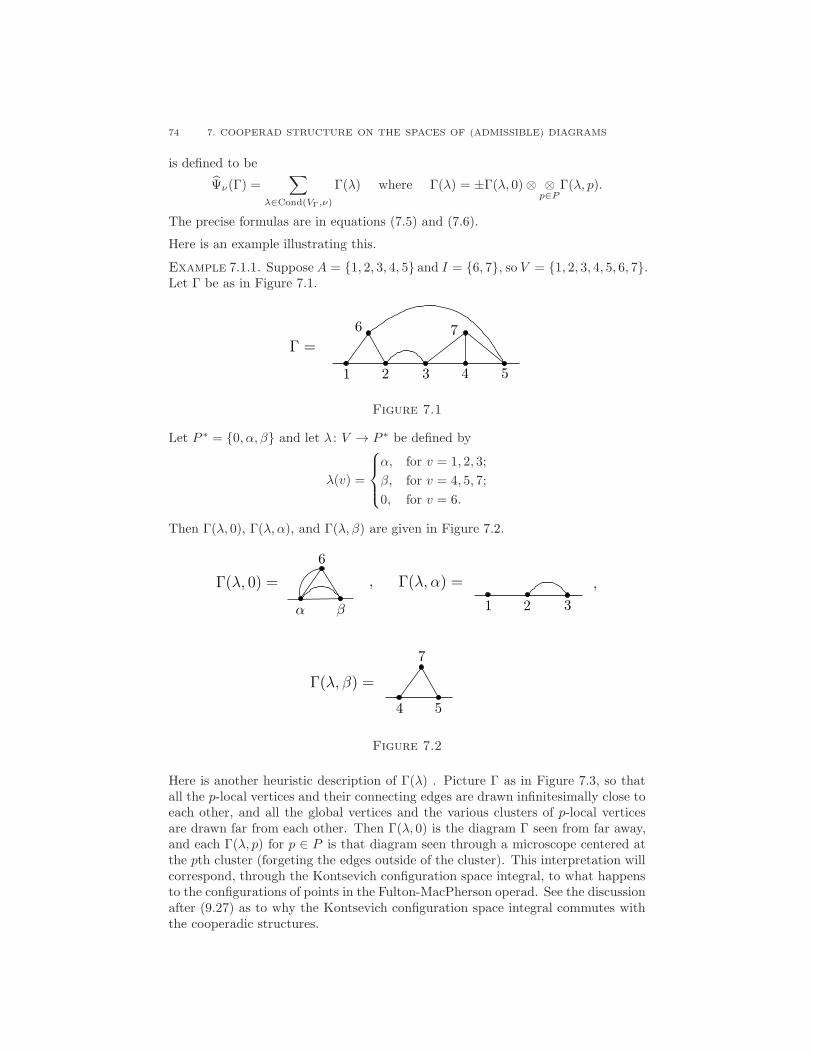
74 7. COOPERAD STRUCTURE ON THE SPACES OF (ADMISSIBLE) DIAGRAMS

is defined to be

Ψν(Γ) =∑

λ∈Cond(VΓ,ν)

Γ(λ) where Γ(λ) = ±Γ(λ, 0)⊗ ⊗p∈P

Γ(λ, p).

The precise formulas are in equations (7.5) and (7.6).

Here is an example illustrating this.

Example 7.1.1. Suppose A = 1, 2, 3, 4, 5 and I = 6, 7, so V = 1, 2, 3, 4, 5, 6, 7.Let Γ be as in Figure 7.1.

Γ =

3 421 5

6 7

Figure 7.1

Let P ∗ = 0, α, β and let λ : V → P ∗ be defined by

λ(v) =

α, for v = 1, 2, 3;

β, for v = 4, 5, 7;

0, for v = 6.

Then Γ(λ, 0), Γ(λ, α), and Γ(λ, β) are given in Figure 7.2.

,Γ(λ, 0) =

α β

6

321

Γ(λ, α) =

4 5

Γ(λ, β) =

7

,

Figure 7.2

Here is another heuristic description of Γ(λ) . Picture Γ as in Figure 7.3, so thatall the p-local vertices and their connecting edges are drawn infinitesimally close toeach other, and all the global vertices and the various clusters of p-local verticesare drawn far from each other. Then Γ(λ, 0) is the diagram Γ seen from far away,and each Γ(λ, p) for p ∈ P is that diagram seen through a microscope centered atthe pth cluster (forgeting the edges outside of the cluster). This interpretation willcorrespond, through the Kontsevich configuration space integral, to what happensto the configurations of points in the Fulton-MacPherson operad. See the discussionafter (9.27) as to why the Kontsevich configuration space integral commutes withthe cooperadic structures.

7.1. CONSTRUCTION OF THE COOPERAD STRUCTURE MAPS Ψν AND Ψν 75

βα

6

1 2 3 4 5

7

Γ =

Figure 7.3

Definition 7.1.2. Let ν : A → P be a weak ordered partition, let P ∗ = 0< P ,let Γ be a diagram on A and assume that IΓ ∩ P = ∅.

• A condensation λ on Γ is a condensation of VΓ relative to ν as in Defini-tion 5.6.1, that is, it is a map λ : VΓ → P ∗ such that λ|A = ν. We considerthe set Cond(Γ, ν) := Cond(VΓ, ν) of all condensations on Γ relative to ν,and write Cond(Γ) when ν is understood.• The extension to the edges of the condensation λ on Γ is the map

λE : EΓ −→ P ∗

defined by

λE(e) =

λ(sΓ(e)), if λ(sΓ(e)) = λ(tΓ(e)),0, otherwise.

• Given a condensation λ of Γ, a vertex v (respectively an edge e) is p-local,for p ∈ P , if λ(v) = p (respectively λE(e) = p). It is global if λ(v) = 0(respectively λE(e) = 0).

The terminology condensation is motivated in the case of diagrams (as it was in Def-inition 5.6.1 for configurations) by the idea explained right before Definition 7.1.2that the diagram should be pictured as in Figure 7.3 with its vertices condensedinto clusters depending on the values of λ.

Clearly the set of condensations on Γ is in bijective correspondence with the set ofmaps from IΓ to P ∗, since the value of a condensation λ on an external vertex ais determined by λ(a) = p for a ∈ Ap, that is, λ(a) = ν(a). An edge is p-local ifand only if both of its endpoints are. Otherwise it is global. Also, a global vertexis always internal but a global edge can be a chord.

Let Γ be a diagram on A and let λ ∈ Cond(Γ). Without loss of generality we canassume that IΓ ∩ P = ∅ (see Remark 6.1.3). For p ∈ P ∗ we define a diagram

(7.1) Γ(λ, p) := (Ap, Ip, Ep, sp, tp)

with

• Ip = IΓ ∩ λ−1(p);

• Ep = λ−1E (p);

• – For p ∈ P , sp and tp are the restrictions of sΓ and tΓ to Ep;


– For p = 0, s0 = λ sΓ and t0 = λ tΓ where

λ : VΓ −→ P ∪ I0

is defined by λ(v) = v if λ(v) = 0, and λ(v) = λ(v) otherwise.

The set of edges (respectively of internal vertices) of Γ is the disjoint union forp ∈ P ∗ of the set of edges (respectively of internal vertices) of the diagrams Γ(λ, p).

Even if Γ is admissible, Γ(λ, p) may not be. Note also that λ above is the same asin (5.22).

The equivalence class of Γ(λ, p) in D(Ap) with respect to the relation ≃ of Defini-tion 6.2.2, or even ⊗p∈P∗Γ(λ, p), is not an invariant of the equivalence class of Γ in

D(A). To correct this we introduce some signs. Define for I = IΓ and E = EΓ,

S(I, λ) := (v, w) ∈ I × I : v < w and λ(v) > λ(w)(which was already introduced in (5.33)), and

S(E, λ) := (e, f) ∈ E × E : e < f and λE(e) > λE(f).Define the signs

σ(I, λ) := (−1)N ·|S(I,λ)| ,(7.2)

σ(E, λ) := (−1)(N−1)·|S(E,λ)| , and(7.3)

σ(Γ, λ) := σ(I, λ) · σ(E, λ)(7.4)

(The sign σ(I, λ) was already defined in (5.32).) The proof of the following isstraightforward.

Lemma 7.1.3. For a diagram Γ and a condensation λ on Γ, the element

σ(Γ, λ) · ⊗p∈P∗

Γ(λ, p) ∈ ⊗p∈P∗D(Ap)

depends only on the equivalence class of Γ in D(A).

For a diagram Γ on A and a condensation λ of Γ we set

(7.5) Γ(λ) := σ(Γ, λ) · ⊗p∈P∗

Γ(λ, p) ∈ ⊗p∈P∗D(Ap),

where σ(Γ, λ) = ±1 is from (7.4) and Γ(λ, p) is from (7.1). By Lemma 7.1.3 we geta linear map

Ψν : D(A) −→ ⊗p∈P∗D(Ap)

defined on generators by

(7.6) Ψν(Γ) :=∑

λ∈Cond(Γ,ν)

Γ(λ).

Recall N (Ap) ⊂ D(Ap), the differential ideal of non-admissible diagrams (Defini-tion 6.5.1 and Lemma 6.5.2). Set

(7.7) N (ν) :=∑

p∈P∗

⊗q∈P∗

q<p

D(Aq)⊗N (Ap)⊗ ⊗q∈P∗

q>p

D(Aq),

7.2. Ψν AND Ψν ARE MORPHISMS OF ALGEBRAS 77

which is a differential ideal in ⊗p∈P∗D(Ap). Since D(Ap) = D(Ap)/N (Ap), we havean isomorphism of CDGAs (Z-graded if N = 2)

(7.8)

(⊗

p∈P∗D(Ap)

)/N (ν) ∼= ⊗

p∈P∗D(Ap)

Lemma 7.1.4. Ψν(N (A)) ⊂ N (ν).

Proof. Let Γ be a non-admissible diagram on A and let λ ∈ Cond(Γ).

• If Γ has a loop at a vertex v, then Γ(λ, λ(v)) also has a loop.• If Γ has double edges e1 and e2, then so does Γ(λ, λE(e1)).• If Γ has an internal vertex v of valence ≤ 2, then the same is true forΓ(λ, λ(v)) because the valence of v can only decrease.• If, for some p ∈ P , Γ has an internal p-local vertex that is not connected toany external vertex, then the same is true for Γ(λ, p). If Γ has a connectedcomponent consisting only of internal global vertices, then the same is truefor Γ(λ, 0).

In all cases we see that if Γ is not admissible, then the same is true for Γ(λ, p) for

some p ∈ P ∗. Therefore Γ(λ) ∈ N (ν) and Ψν(N (A)) ⊂ N (ν).

Proposition 7.1.5. Ψν defined in (7.6) induces a linear map

Ψν : D(A) −→ D(P ) ⊗ ⊗p∈PD(Ap).

Proof. This is an immediate consequence of the isomorphism (7.8) andLemma 7.1.4.

Thus, for an admissible diagram Γ, Ψν(Γ) is obtained as the sum (7.6) in whichnon-admissible terms are set to zero. Actually, there are many condensations λfor which Γ(λ) is not admissible and therefore does not contribute to Ψν(Γ). Inparticular, only admissible condensations (to be defined in Definition 7.3.3) cancontribute to the sum, and hence we can use the sum (7.11) below, which has manyfewer terms, to define Ψν(Γ).

7.2. Ψν and Ψν are morphisms of algebras

The aim of this section is to prove

Proposition 7.2.1. Ψν and Ψν are morphisms of algebras.

Proof. We first prove the statement for Ψν . Let Γ1 and Γ2 be two diagramson A and suppose that IΓ1 and IΓ2 , EΓ1 and EΓ2 respectively, are disjoint.

Define the function

Cond(Γ1)× Cond(Γ2) −→ Cond(Γ1 · Γ2), (λ1, λ2) 7−→ λ1 · λ2

by (λ1 · λ2)(v) = λi(v) when v ∈ VΓi for i = 1, 2. This map is well-defined becauseif v ∈ VΓ1 ∩ VΓ2 then v is external and λ1(v) = λ2(v) = ν(v). Moreover, it is abijection whose inverse is given by λ 7→ (λ|VΓ1 , λ|VΓ2).


Since

Γ1(λ1, p) · Γ2(λ2, p) = (Γ1 · Γ2)(λ1 · λ2, p)

it is easy to see that

⊗p∈P∗

(Γ1 · Γ2)(λ1 · λ2, p) = η(Γ1, λ1,Γ2, λ2) ·(⊗

p∈P∗Γ1(λ1, p)

)·(⊗

q∈P∗Γ2(λ2, q)

).

where

η(Γ1, λ1,Γ2, λ2) := (−1)s with s =∑

p,q∈P∗

q<p

deg(Γ1(λ1, p)) · deg(Γ2(λ2, q)).

We have

Ψν(Γ1 · Γ2) =∑

λ∈Cond(Γ1·Γ2)

σ(Γ1 · Γ2, λ) · ⊗p∈P∗

(Γ1 · Γ2)(λ, p)

=∑

λ1∈Cond(Γ1)

∑

λ2∈Cond(Γ2)

σ(Γ1 · Γ2, λ1 · λ2) · ⊗p∈P∗

(Γ1 · Γ2)(λ1 · λ2, p)

=∑

λ1∈Cond(Γ1)

∑

λ2∈Cond(Γ2)

σ(Γ1 · Γ2, λ1 · λ2) · η(Γ1, λ1,Γ2, λ2)(7.9)

·(⊗

p∈P∗Γ1(λ1, p)

)·(⊗

q∈P∗Γ2(λ2, q)

)

On the other hand

Ψν(Γ1) · Ψν(Γ2) =∑

λ1∈Cond(Γ1)

∑

λ2∈Cond(Γ2)

Γ1(λ1) · Γ2(λ2)

=∑

λ1∈Cond(Γ1)

∑

λ2∈Cond(Γ2)

σ(Γ1, λ1) · σ(Γ2, λ2)(7.10)

·(⊗

p∈P∗Γ1(λ1, p)

)·(⊗

q∈P∗Γ2(λ2, q)

)

It remains to check that the signs of (7.9) and (7.10) agree, which is straightforward..

For Ψν , the statement is a consequence of the definition of Ψν in Proposition 7.1.5and of the fact that (7.8) is an isomorphism of algebras.

7.3. Ψν is a chain map

This section is devoted to the proof of the following

Proposition 7.3.1. Ψν commutes with the differentials.

The analog for Ψν is not true, as illustrated in the following example.

Example 7.3.2. Here we will show that Ψν is not a chain map. Consider thediagram Γ given in Figure 7.4, with the set of external vertices A = a. Theinternal vertices 1, 2, 3, 4 have their natural order and each edge is oriented fromthe lower to the higher vertex. Suppose also that N is odd, and hence the order ofedges is irrelevant. Set P = α and consider the unique ordered partition

ν : a −→ α.

7.3. Ψν IS A CHAIN MAP 79

The boundary of Γ is given by the diagram pictured on the top right of Figure 7.4(obtained as an alternating sum of three such diagrams).

Then Ψν(dΓ) is a sum of eight terms corresponding to the eight condensations

λ : 1, 2, 3 −→ P ∗ = 0, α.Using that dead ends are not contractible and diagrams with loops vanish when Nis odd (because of the relations ≃ of Definition 6.2.2), one computes that

d(Ψν(dΓ)) ∈ D(α)⊗ D(a)consists of a single term, corresponding to the condensation λ(1) = α , λ(2) =λ(3) = 0, and represented by the bottom picture of Figure 7.4.

3

,

a

dΓ =

21 3

a

Γ =

23

4

1

,

α

⊗d(Ψν(dΓ)) =

a

1

Figure 7.4. A diagram Γ for which d(Ψνd(Γ)) 6= 0.

Thus

d(Ψνd(Γ)) 6= 0.

On the other hand

d(dΨν(Γ)) = 0

since d2 = 0. Therefore Ψν is not a chain map.

In fact, the equality Ψνd = dΨν is not really expected to hold. Indeed, if Γ is adiagram with l internal vertices then there are l|P |+1 terms in Ψν(Γ), correspondingto the various condensations. On the other hand, for each contractible edge e in Γ,Ψν(Γ/e) has only (l−1)|P |+1 terms. Thus there is no clear correspondence between

the terms of the sums Ψνd(Γ) and of dΨν(Γ), and hence no evidence that these twosums should be equal.

This explains why the proof below that Ψν is a chain map is quite elaborate.The idea is to restrict to condensations of Γ for which Γ(λ) is admissible and toestablish Lemma 7.3.8, which amounts to exhibiting a 1–1 correspondence betweencondensations of Γ and of Γ/e.

Let Γ be a diagram on A.


Definition 7.3.3. A condensation λ of Γ is admissible if for each internal vertex iand each p ∈ P there is an equivalence

λ(i) = p ⇐⇒ i admits at least two distinct adjacent p-local vertices.

Denote by AdmCond(Γ) the set of admissible condensations on Γ.

This terminology is motivated by the following:

Lemma 7.3.4. If λ is not admissible then Γ(λ) ∈ N (ν).

Proof. Suppose that i is a p-local internal vertex for some p ∈ P , and supposethat it does not have two adjacent p-local vertices. Then i is internal of valence< 2 in Γ(λ, p), and hence Γ(λ, p) ∈ N (Ap).

Suppose that i is an internal vertex that is not p-local but that has two adjacentp-local vertices for some p ∈ P . Then in Γ(λ, 0), the external vertex p is connectedby a double edge to either i (if λ(i) = 0) or to the external vertex q (if λ(i) = q ∈P \ p). Thus Γ(λ, 0) ∈ N (P ).

Lemma 7.3.4 implies that, in ⊗p∈P∗D(Ap) and for Γ admissible,

(7.11) Ψν(Γ) =∑

λ∈AdmCond(Γ,ν)

Γ(λ).

Lemma 7.3.5. Let λ1, λ2 be two admissible condensations on Γ. If λ1 and λ2

coincide on all vertices except possibly on one, then λ1 = λ2.

Proof. Let u be a vertex of Γ such that λ1(v) = λ2(v) for v 6= u. If u isexternal then the values of λi(u) are determined by ν, and hence λ1 = λ2. Supposethat u is internal. If u has two adjacent vertices that are p-local (for both λ1 andλ2) for some p ∈ P , then λi(u) = p by admissibility. Otherwise λi(u) = 0, againby admissibility.

For a condensation λ of Γ, recall the extension to vertices λE from Definition 7.1.2and Γ(λ, p) from Equation (7.1).

Definition 7.3.6. An edge e of Γ is λ-contractible if it is contractible in Γ(λ, λE(e)).

Lemma 7.3.7. Assume that Γ is admissible and let λ be an admissible condensation.An edge e of Γ is λ-contractible if and only if the following conditions hold:

(1) e is contractible in Γ, and(2) λ(sΓ(e)) = λ(tΓ(e)) or min(λ(sΓ(e)), λ(tΓ(e))) = 0.

Condition (2) of the lemma is equivalent to having either both endpoints of e p-localfor some p ∈ P or some endpoint being global.

Proof. First we show that (1) and (2) are necessary conditions. If (1) doesnot hold then e is a chord in Γ (because Γ is admissible). Therefore e is also achord in Γ(λ, λE(e)), and hence it is not λ-contractible. If (2) does not hold then eis a chord in Γ(λ, 0) joining the external vertices λ(sΓ(e)) and λ(tΓ(e)). Thereforee is not λ-contractible.


Suppose now that (1) and (2) hold. We will prove that e is a contractible edge inΓ(λ, λE(e)). Let v and w be the endpoints of e. As Γ is admissible, e is not a loopand v 6= w. We distinguish three cases.

• Case 1: λ(v) = λ(w) = p ∈ P .Since e is contractible, v or w is internal in Γ, and hence the same istrue in Γ(λ, p). Clearly e is neither a chord, nor a loop there. Since λ isadmissible, if v is internal, then it has an adjacent p-local vertex, distinctfrom w. Therefore v also has another adjacent vertex in Γ(λ, p). The sameis true for w if it is internal. Therefore e is not a dead end in Γ(λ, p). Thuse is λ-contractible.• Case 2: λ(v) = λ(w) = 0.Then e is an edge of Γ(λ, 0) joining two distinct internal vertices v and w.In particular e is neither a chord nor a loop. Since e is not a dead end inΓ, there exists a vertex v′ 6= w that is adjacent to v in Γ. If v′ is globalthen it is also a vertex of Γ(λ, 0) and if v′ is p-local, for some p ∈ P , thenit becomes an external vertex p in Γ(λ, 0). In both cases in Γ(λ, 0), v hasan adjacent vertex distinct from w. Similarly w has an adjacent vertex inΓ(λ, 0) distinct from v. Therefore e is not a dead end in Γ(λ, 0) and e isλ-contractible.• Case 3: λ(v) = 0 and λ(w) = p ∈ P (or the other way).Then e is an edge of Γ(λ, 0) joining the internal vertex v to the externalvertex p. Since e is not a dead end in Γ, there is a vertex v′ adjacent to vin Γ and distinct from w. Since λ is admissible, we have that λ(v′) 6= p,and hence v′ is either global, or q-local for some q 6= p. Then, in Γ(λ, 0),v′ either is an internal vertex or becomes the external vertex q. In bothcases it is a vertex distinct from p and adjacent to v. This proves that eis not a dead end. Thus e is λ-contractible.

Let e be a contractible edge in Γ. Let v and w be the endpoints of e with v < w.Thus VΓ/e = VΓ \ w. Define the function

(7.12) λ/e : VΓ/e −→ P ∗

by

(λ/e)(z) =

λ(z), if z 6= v or z = v is external;max(λ(v), λ(w)), if z = v is internal.

It is clear that λ/e is a condensation of Γ/e. Notice also that if e is λ-contractiblethen (λ/e)(v) = max(λ(v), λ(w)).

Assume that Γ is an admissible diagram. Consider the sets


Ω =(e, λ) : e ∈ EΓ, λ ∈ AdmCond(Γ), e λ-contractible,

(Γ/e)(λ/e) 6= 0 in ⊗p∈P∗

D(Ap),

Ω =(e, λ) : e ∈ EΓ, e contractible, λ ∈ Cond(Γ/e),

(Γ/e)(λ) 6= 0 in ⊗p∈P∗ D(Ap),

and the map

ω : Ω −→ Ω

(e, λ) 7−→ (e, λ/e).

Lemma 7.3.8. ω is a bijection.

Proof. We first show that ω is injective. Let e be a contractible edge and, fori = 1, 2, let λi be admissible condensations of Γ such that e is λi-contractible and(Γ/e)(λi/e) 6= 0. Assume that λ1/e = λ2/e. We will show that λ1 = λ2.

Set λ = λ1/e = λ2/e. This is an admissible condensation because (Γ/e)(λ) 6= 0 in⊗p∈P∗D(Ap) and because of Lemma 7.3.4. Let v and w be the endpoints of e withv < w. Thus VΓ/e = VΓ \ w. We know that λi agrees with λ on VΓ \ v, w, andtherefore we only need to show that λ1(v) = λ2(v) and λ1(w) = λ2(w). Moreover,since each λi is admissible, by Lemma 7.3.5 it is enough to prove only one of thesetwo equations.

If v is external, then λ1(v) = λ2(v) is determined and hence λ1 = λ2. Supposethat v is internal. If λ(v) = 0 then, since λ(v) = max(λi(v), λi(w)), we get λi(v) =λi(w) = 0 for i = 1, 2, and hence λ1 = λ2. Suppose that λ(v) = p ∈ P . Byadmissibility of λ, there exist two vertices x and y other than v and w that areadjacent to v in Γ/e and with λ(x) = λ(y) = p. This implies that λi(x) = λi(y) = pfor i = 1, 2. Then in Γ, either x and y are both adjacent to v (respectively tow), or x is adjacent to v and y is adjacent to w (or the other way around). Inthe first case we get by admissibility of λi that λ1(v) = λ2(v) = p (respectivelyλ1(w) = λ2(w) = p), and hence λ1 = λ2 by Lemma 7.3.5. In the second case, sincep = λ(v) = max(λ1(v), λ1(w)), we get that λ1(v) = p or λ1(w) = p. Let us saythat λ1(v) = p, the other case being analogous. Then w is adjacent to v and toeither x or y, and thus w is adjacent to two p-local vertices (for the condensationλ1), and hence we also have λ1(w) = p by admissibility. The same argument showsthat λ2(v) = λ2(w) = p. This proves injectivity of ω.

To show ω is surjective, let e be a contractible edge of Γ and let λ be a condensationof Γ/e such that (Γ/e)(λ) 6= 0. We will construct an admissible condensation λ of Γsuch that e is λ-contractible and λ/e = λ. Let v and w again be the endpoints of ewith v < w. For z ∈ VΓ \ v, w, set λ(z) = λ(z). We need to define λ(v) and λ(w)and to check that λ has the desired properties. We consider the following cases.

(1) Suppose v is external. Then λ(v) = λ(v) = p ∈ P is prescribed by ν.(a) Suppose that there exists a vertex x in Γ different from v and adjacent

to w such that λ(x) = p. In that case, set λ(v) = λ(w) = p. Then


λ is admissible at the vertex w because it has two p-local adjacentvertices v and x. It is easy to check that λ is also admissible at theother internal vertices of Γ, using the fact that λ is. Moreover e is λ-contractible by Lemma 7.3.7 since it is contractible and λ(v) = λ(w).

(b) Suppose that w is not adjacent to any p-local vertex other than v. Inthat case, set λ(v) = p and λ(w) = 0. The vertex w is not adjacent inΓ to two vertices x and y such that λ(x) = λ(y) = q ∈ P with q 6= pbecause otherwise (Γ/e)(λ, 0) would contain a double edge joiningp and q, and hence Γ/e ∈ N (ν), contrary to our hypothesis. Thisproves that λ is admissible at w and the admissibility at other verticesis a consequence of the admissibility of λ. Also e is λ-contractible.

(2) Suppose that v is internal. Then w is also internal since v < w.(a) Suppose that λ(v) = 0. In that case set λ(v) = λ(w) = 0. By

admissibility of λ, there do not exist two vertices x, y ∈ VΓ \ v, wadjacent in Γ to either v or w with λ(x) = λ(y) ∈ P . It is easy to seethat λ is admissible and e is λ-contractible.

(b) Suppose that λ(v) = p ∈ P . By admissibility of λ there exist twodistinct vertices x, y ∈ VΓ \ v, w adjacent in Γ to either v or w suchthat λ(x) = λ(y) = p.• If v is not adjacent to any vertices in (VΓ \ v, w) ∩ λ−1(p)

then set λ(v) = 0 and λ(w) = p.• If w is not adjacent to any vertices in (VΓ \ v, w) ∩ λ−1(p)

then set λ(v) = p and λ(w) = 0.• If both v and w are adjacent to some vertices in (VΓ \ v, w)∩

λ−1(p) then set λ(v) = λ(w) = p.In each case it is easy to see that λ is admissible and that e is λ-contractible.

This proves surjectivity of ω.

Lemma 7.3.9. If Γ is admissible, if λ is admissible, and if e is a λ-contractible edgeof Γ, then, for p ∈ P ∗, we have in D(Ap):

(Γ/e)(λ/e, p) =

Γ(λ, p)/e, if p = λE(e);Γ(λ, p), otherwise.

Proof. Let v and w be the endpoints of e with v < w. Then VΓ/e = VΓ \ wand EΓ/e = EΓ \ e. It is easy to see that the equations to prove are equivalent to

λ/e = λ|(VΓ \ w)

(λ/e)E = λE |(EΓ \ e)

Since e is λ-contractible, by Lemma 7.3.7, λ(v) = λ(w) or min(λ(v), λ(w)) = 0.If λ(v) < λ(w) then λ(v) = 0 which implies that v is internal, and the same forw because v < w, in which case we can transpose the order of v and w to getan equivalent diagram (up to sign) in which the roles of v and w are exchanged.Therefore, without loss of generality we can always assume that λ(v) ≥ λ(w). Thisimplies that (λ/e)(v) = λ(v). Also for z 6= v, w we have (λ/e)(z) = λ(z). Thusλ/e = λ|VΓ \ w.


It remains to prove that (λ/e)E = λE |(EΓ \ e). Let f 6= e be an edge of Γ. If wis not an endpoint of f , then, since λ/e = λ|VΓ \ w, (λ/e)E(f) = λE(f). Supposethat w is an endpoint of f . If λ(w) = λ(v) then (λ/e)E(f) = λE(f). Otherwiseλ(w) = 0 and λ(v) = p ∈ P , and hence f is global in Γ. As Γ is admissible andf 6= e, the other endpoint of f is not v. Since λ is admissible and since w is notr-local but is adjacent to the p-local vertex v, we get that the other endpoint of f isnot p-local. This implies that f is global in Γ/e, and hence (λ/e)E(f) = λE(f) = 0.This proves that (λ/e)E = λE |(EΓ \ e).

Proof of Proposition 7.3.1. Let Γ be an admissible diagram on A. Forp ∈ P ∗ and for a condensation λ of Γ, define the sign

η(Γ, λ, p) := (−1)s with s =∑

q∈P∗

q<p

deg(Γ(λ, q)).

We have

d(Ψν(Γ))(7.11)= d

∑

λ∈AdmCond(Γ)

Γ(λ)

=∑

λ∈AdmCond(Γ)

∑

p∈P∗

σ(Γ, λ) · η(Γ, λ, p)·(7.13)

· ⊗q<p

Γ(λ, q)⊗ d (Γ(λ, p))⊗ ⊗q>p

Γ(λ, q)

=∑

λ∈AdmCond(Γ)

∑

p∈P∗

∑

e∈EcontrΓ(λ,p)

σ(Γ, λ) · η(Γ, λ, p) · ǫ(Γ(λ, p), e)·

· ⊗q<p

Γ(λ, q)⊗ Γ(λ, p)/e⊗ ⊗q>p

Γ(λ, q)

Lemma 7.3.9=

∑

(e,λ)∈Ω

σ(Γ, λ) · η(Γ, λ, λE(e)) · ǫ(Γ(λ, λE(e)), e)·(7.14)

·(⊗

p∈P∗(Γ/e)(λ/e, p)

).(7.15)

On the other hand,

Ψν(d(Γ)) = Ψν

∑

e∈EcontrΓ

ǫ(Γ, e) · Γ/e

=∑

(e,λ)∈Ω

ǫ(Γ, e) · σ(Γ/e, λ) ·(⊗

p∈P∗(Γ/e)(λ, p)

)

Lemma 7.3.8=

∑

(e,λ)∈Ω

ǫ(Γ, e) · σ(Γ/e, λ/e) ·(⊗

p∈P∗(Γ/e)(λ/e, p)

)(7.16)

It remains to check that the signs of (7.15) and (7.16) agree, which is straighforward.

7.4. PROOF THAT THE COOPERAD STRUCTURE IS WELL-DEFINED 85

7.4. Proof that the cooperad structure is well-defined

We show in this section that Ψν and Ψν endow D and D with the cooperadicstructure (the former in the category of vector spaces and the latter in the categoryof chain complexes), when ν runs over all weak ordered partitions.

First let us show the associativity of the structure maps. Suppose given a weakordered partition ν : A → P as before. Suppose moreover that A is itself linearlyordered, that ν is increasing, and that P ∗ ∩ A = ∅. Let ξ : B → A be an orderedweak partition of a finite set B. Set Ba = ξ−1(a) for a ∈ A. Also set A∗ = 0<A.

We then have a natural bijection

∐a∈A

Ba∼= ∐

p∈P∐

a∈Ap

Ba.

For p ∈ P , the partition ξ restricts to a weak ordered partition

ξp : ∐a∈Ap

Ba −→ Ap.

The associativity of Ψ amounts to the following lemma whose proof is straightfor-ward.

Lemma 7.4.1. The following diagram is commutative:(7.17)

D(∐

p∈P

(∐

a∈Ap

Ba

))

Ψνξ

D(∐

a∈ABa

)

Ψξ

D(P )⊗ ⊗

p∈PD(∐

a∈Ap

Ba

)

id⊗ ⊗p∈P

Ψξp

D(A) ⊗ ⊗a∈AD(Ba)

Ψν⊗id

D(P )⊗ ⊗p∈P

(D(Ap)⊗ ⊗

a∈Ap

D(Ba)

)∼=

τ//(D(P )⊗ ⊗

p∈PD(Ap)

)⊗ ⊗

a∈AD(Ba)

The horizontal bottom isomorphism τ is the obvious reordering of factors (with theusual Koszul sign).

We next define an action of the group Perm(A) of permutation of the finite set A ondiagrams on A. Given a permutation σ ∈ Perm(A) and a diagram Γ = (A,E, I, s, t),we define a new diagram

σ · Γ = (A,E, I, σ s, σ t)where the bijection σ : A

∼=−→ A is extended to all vertices by σ(i) = i for i ∈ I.The following is immediate.

Proposition 7.4.2. There is an induced action of (Z-graded) CDGA of Perm(A)

on D(A) and D(A).

To define the counits of the cooperad structure, consider the CDGA maps

η : D(1) −→ K and η : D(1) −→ K


defined by η(1) = 1 and η(Γ) = 0 for a diagram other than the unit, and similarlyfor η.

Theorem 7.4.3. The structure maps Ψν and Ψν , for all weak ordered partitions ν,the symmetric action, and the counits η and η described above define:

• the structure of a cooperad of Z-graded K-algebras on D, and• the structure of a cooperad of CDGAs on D (Z-graded if N = 2).

Proof. The associativity of the structure maps Ψ required for a cooperadstructure is exactly Lemma 7.4.1. We have the corresponding associativity for Ψ

since, by Proposition 7.1.5, that structure map is induced by Ψ. It is easy to checkthat η and η are counits. The equivariance is also easy to check.

Note that the cooperad structures developed here are related to cooperad strucureson the category of sets (as developed in [29]).

CHAPTER 8

Equivalence of the cooperads D and H∗(C[•])

We show in this chapter that the CDGA cooperad D of admissible diagrams isweakly equivalent to the cohomology algebra of the Fulton-MacPherson cooperadH∗(C[•];K) for any commutative ring with unit K and ambient dimension N ≥ 2.

Fix a finite set A. We first recall the computation of the algebra H∗(C[A];K) due

to F. Cohen [10]. Denote by [vol] ∈ HN−1(SN−1;K) the orientation class of thesphere. For a, b which are distinct in A, recall the map θab : C[A] → SN−1 from(5.6) which gives the direction between two points of the configuration, and set

(8.1) gab := θ∗ab([vol]) ∈ HN−1(C[A];K).

Then as graded algebras we have

H∗(C[A];K) =∧ (gab : a, b ∈ A, a 6= b)

(3-term relation ; (gab)2 ; gab − (−1)Ngba)

where ∧(gab) is the free commutative graded K-algebra generated by the gab’s,and the 3-term relation is

gabgbc + gbcgca + gcagab

for all distinct a, b, c ∈ A. Here we follow the standard conventions in rationalhomotopy theory and denote by ∧Z the free commutative graded algebra generatedby a graded vector space Z. This is thus the tensor product of the symmetric algebraon Zeven and the exterior algebra on Zodd.

For a, b distinct in A, denote by

(8.2) Γ〈a, b〉the diagram on A with no internal vertices and whose only edge is a chord from ato b. This is an admissible cocycle of degree N − 1.

We endow the cohomology algebra with a zero differential to make it a CDGA.

Theorem 8.1. For N ≥ 2, there is a quasi-isomorphism of CDGAs (Z-graded ifN = 2)

I : D(A) ≃−→ (H∗(C[A];K), 0)

characterized byI(Γ〈a, b〉) = gab, for a, b distinct in A;

I(Γ) = 0, for a diagram Γ with internal vertices.

Moreover I is a weak equivalence of cooperads.

87

88 8. EQUIVALENCE OF THE COOPERADS D AND H∗(C[•])

The rest of the chapter is devoted to the proof of this theorem.

Consider the submodule D(0)(A) of D(A) generated by admissible diagrams withoutinternal vertices. Then

D(0)(A) =∧ (Γ〈a, b〉 : a, b ∈ A, a 6= b)

((Γ〈a, b〉)2 ; Γ〈a, b〉 − (−1)NΓ〈b, a〉) .

Therefore we have a surjective algebra map

I0 : D(0)(A) −→ H∗(C[A];K)

defined by I0(Γ〈a, b〉) = gab.

Lemma 8.2.

I0(D(0)(A) ∩ d(D(A))) = 0.

Proof. It is enough to prove that I0(dΓ) = 0 when Γ is an admissible diagramconsisting of one internal vertex i and n edges connecting it to the external verticesa1, . . . , an. In that case,

I0(dΓ) =

n∑

k=1

(−1)kga1akga2ak

. . . gak−1akgakak+1

. . . gakan .

The right side vanishes as can be seen using an easy induction on n ≥ 3 and the3-term relation

ga1akga2ak

= ga1a2(ga2ak− ga1ak

).

from (1.3) (which corresponds to the case n = 3).

When K = R, an alternative non-computational proof is possible: The Kontsevichconfiguration space integral

I : D(n)→ ΩPA(C[n])

(to be defined in Chapter 9) commutes with the differential (Proposition 9.4.1),and hence

I0(dΓ) = [I(dΓ)] = [dI(Γ)] = 0

in H(ΩPA(C[n])) ∼= H∗(C[n];R).

This lemma implies that we can define the CDGA morphism I by

(8.3) I(Γ) =

I0(Γ), if Γ has no internal vertices;

0, otherwise.

It is straightforward to check that this induces a morphism of cooperads.

Since I induces a surjection in homology, in order to prove that it is a quasi-isomorphism we only need to establish the following

Lemma 8.3. The graded K-modules H∗(D(A)) and H∗(C[A];K) are isomorphic.

The proof of this lemma will take up the rest of this chapter.

A diagram Γ on A induces a partition of A into its path-connected components,and we denote this partition by νΓ. In other words, two external vertices a and bbelong to the same element C ∈ νΓ (see Definition 2.3.1 for definitions regarding

8. EQUIVALENCE OF THE COOPERADS D AND H∗(C[•]) 89

partitions) if and only if they are connected by a path of unoriented edges in Γ.For a partition ν of A, denote by

D(A)〈ν〉the submodule of D(A) generated by admissible diagrams Γ whose partition ofconnected components is ν. It is clear that D(A)〈ν〉 is a subcomplex of D(A). Inthe particular case of the indiscrete partition ν = A, we get the subcomplex ofconnected admissible diagrams

D˜(A) := D(A)〈A〉.

We have an isomorphism of complexes

(8.4) D(A) ∼= ⊕ν⊗

C∈νD˜(C)

where the sum runs over all partitions ν of the set A.

The Poincare series of the homology of the configuration space C[A] is given by[10]

(8.5) (1 + t)(1 + 2t) . . . (1 + (|A| − 1)t)

with t of degree N − 1. In particular the top degree Betti number is

(8.6) dimH(N−1)(|A|−1)(C(A);K) = (|A| − 1)!

In view of the isomorphism (8.4) and formulas (8.5) and (8.6), Lemma 8.3 will bea direct consequence of the following

Lemma 8.4. For A non-empty,

dimHi(D˜(A)) =

(|A| − 1)!, if i = (N − 1) · (|A| − 1),0, otherwise.

Before proving this lemma, we introduce further submodules. Fix an element a ∈ Aand consider the following submodules of D

˜(A):

• U0 is the submodule generated by connected admissible diagrams with aof valence 1 and such that the only edge with endpoint a is contractible;• U1 is the submodule generated by connected admissible diagrams with aof valence ≥ 2;• D˜′(A) is the submodule generated by all connected admissible diagrams

that are neither in U0 nor in U1.

It is clear that D˜′(A) is a subcomplex of D

˜(A).

Lemma 8.5. The inclusion

D˜′(A) → D

˜(A)

is a quasi-isomorphism.

Proof. Consider the quotient complex U := D˜(A)/D

˜′(A). We need to show

that U is acyclic.

Identify U in the obvious way with the graded K-module U0⊕U1, and define an in-creasing filtration on U where elements of filtration ≤ p are the linear combinationsof diagrams in U0 with less than p edges and diagrams in U1 with less than p − 1

90 8. EQUIVALENCE OF THE COOPERADS D AND H∗(C[•])

edges. The differential preserves the filtration. Consider the spectral sequence asso-ciated to this filtration and which converges to the homology of U . The differentialat the 0th page

d0 : U0 −→ U1consists of contracting the only edge with endpoint a. It is an isomorphism becausethere is an inverse given by “blowing up” the vertex a of a diagram Γ ∈ U1 intoa contractible edge (a, a′) as in Figure 8.1. Therefore the page E1 of the spectralsequence is trivial and hence U is acyclic.

3 42a=1

5

a′

3 42a=1

5

Figure 8.1. Example of blowing up vertex a = 1 into a con-tractible edge (a, a′).

We are now ready for the

Proof of Lemma 8.4. The proof is by induction on the cardinality of A.

If A is a singleton then D˜′(A) = K · 1, where 1 is the unit diagram with a single

external vertex and no internal vertices or edges. Lemma 8.4 is then a consequenceof Lemma 8.5.

Let A be of cardinality k ≥ 2 and suppose that the lemma has been proved for< k external vertices. Fix a ∈ A. Any diagram in D

˜′(A) has exactly one edge with

endpoint a and it is a chord. We have an isomorphism of complexes

D˜′(A) ∼= ⊕

b∈A\aΓ〈a, b〉 · D

˜(A \ a).

Using Lemma 8.5 we conclude that

dimHi(D˜(A)) = (|A| − 1) · dimHi−(N−1)(D

˜(A \ a))

and deduce the desired conclusion using the induction hypothesis.

We now finish the

Proof of Lemma 8.3. An elementary computation by induction on |A| usingisomorphism (8.4) and Lemma 8.4 shows that the Poincare series of H∗(D(A)) isexactly (8.5), and this is also the Poincare series of H∗(C[A]).

This finishes the proof of Theorem 8.1.

CHAPTER 9

The Kontsevich configuration space integrals

In the previous chapter we built a quasi-isomorphism

I: D(n) ≃−→ H∗(C[n])

of cooperads. The goal of this section is to construct a CDGA morphism

I: D(n) −→ ΩPA(C[n])

which will turn out to be a quasi-isomorphism as well as “almost” a morphism ofcooperads (see Proposition 9.5.1 below for the precise meaning of this.) In thisentire chapter the ground ring is the field of real numbers K = R. We also fixan integer N ≥ 2 which is the dimension of the euclidean space RN on which weconsider the configuration spaces C[n], as well as the underlying dimension of thespace of admissible diagrams D = DN .

We will throughout use many constructions related to semi-algebraic forms that wequickly reviewed in Chapter 4 and which are fully developed in [19].

The plan of this chapter is as follows.

9.1: We construct a linear map

I : D(n) −→ ΩPA(C[n]).

9.2: We prove that I is a map of algebras.

9.3: We show that I induces the desired map I on D(n) by showing that itvanishes on non-admissible diagrams.

9.4: We prove that I, and hence I, commutes with the differentials.

9.5: We prove that I and I are almost morphisms of cooperads.

Before reading on, the reader might want to look at the last part of the introductionwhere some intuition about the integrals defined in this chapter is given.

9.1. Construction of the Kontsevich configuration space integral I

Fix a finite set A. We construct a linear map

I : D(A) −→ ΩPA(C[A])

as follows.

Let Γ be a diagram on A. Let vol be the standard normalized volume form on thesphere SN−1 ⊂ RN defined as

(9.1) vol = κN ·N∑

i=1

(−1)iti dt1 ∧ · · · ∧ dti ∧ · · · ∧ dtN

91

92 9. THE KONTSEVICH CONFIGURATION SPACE INTEGRALS

where t1, . . . , tN are the standard coordinates in RN , dti means dti is omitted, andκN ∈ R is a normalizing constant such that

ˆ

SN−1

vol = 1.

Since all the functions in (9.1) are polynomials, and are hence semi-algebraic, vol ∈ΩN−1

min (SN−1) is what was called in Chapter 4 a minimal form. More generally, forany linearly ordered finite set E, consider the product of spheres

(SN−1)E =∏

e∈E

SN−1,

and denote by volE the top volume form in that product, that is,

(9.2) volE := ×e∈E vole ∈ Ωmin((SN−1)E)

where the products are taken in the order of E and vole is the standard normalizedvolume form on the eth factor.

For v and w two distinct vertices in VΓ, recall from (5.6) the map

θv,w : C[VΓ] −→ SN−1

which associates to a configuration x the direction from x(v) to x(w). By conven-tion, when v = w, we set θv,v to be the constant map to a fixed basepoint of thesphere. For an edge e of Γ we set θe = θsΓ(e),tΓ(e) and we define

θΓ := (θe)e∈EΓ: C[VΓ] −→ (SN−1)EΓ .

Recall the definition of a minimal form from Equation (4.3). We then have such aform

(9.3) θ∗Γ(volEΓ) ∈ Ωmin(C[VΓ])

which is of degree l = |EΓ| · (N − 1).

By Theorem 5.3.2, the canonical projection

(9.4) πΓ : C[VΓ] −→ C[A]

is an oriented SA bundle. When |A| ≥ 2, the fiber of πΓ is of dimension N · |IΓ|and integration along the fiber [19, Definition 8.3] gives a pushforward map

(9.5) (πΓ)∗ : Ωlmin(C[VΓ]) −→ Ω

l−N ·|IΓ|PA (C[A]).

When |A| ≥ 2, define I(Γ) as the pushfoward

(9.6) I(Γ) := (πΓ)∗(θ∗Γ(volEΓ)) ∈ ΩPA(C[A]).

For example when Γ is the diagram from Figure 1.2 in the Introduction, I(Γ) cor-responds to formula (1.8).

If A is empty or a singleton we just set

(9.7) I(Γ) :=

1, if Γ is the unit diagram;

0, otherwise.

The reason we treat the case |A| ≤ 1 separately is that the dimension of thefiber of πΓ is then smaller than expected when there are internal vertices (see

9.2. I IS A MORPHISM OF ALGEBRAS 93

Theorem 5.3.2). Therefore we should in those cases consider the pushforward πΓ∗

of (9.5) to be 0. Formula (9.7) is a clean way to do this.

Lemma 9.1.1. For any finite set A, formulas (9.6) and (9.7) induce a degree 0linear map

I : D(A) −→ ΩPA(C[A]).

Proof. This is clear for |A| ≤ 1. Suppose that |A| ≥ 2. It is easy to checkthat (9.6) is compatible with the equivalence relation ≃ of Definition 6.2.2 (it is the

compatibility with I which is the motivation for the definition of ≃). We extend it

by linearity. It is clear that I is of degree 0 (recall Definition 6.2.3 of the degree ofa diagram).

9.2. I is a morphism of algebras

In this section we prove

Proposition 9.2.1. I is a morphism of algebras.

Proof. If |A| ≤ 1 then the proposition is obvious. Suppose now that |A| ≥ 2.Let Γ1 and Γ2 be two diagrams on A and suppose, without loss of generality, thatthey have disjoint sets of internal vertices and of edges. Notice that VΓ1·Γ2 =VΓ1 ∪A VΓ2 and consider the pullback

(9.8) Csing[VΓ1 , VΓ2 ]

q1

q2 //

pullback

C[VΓ2 ]

π2

C[VΓ1 ]

π1 // C[A]

which defines a singular configuration space as in Section 5.5.

Set π′ = πi qi : Csing[VΓ1 , VΓ2 ]→ C[A]. Consider the canonical projections

π : C[VΓ1·Γ2 ] −→ C[A]

and

ρi : C[VΓ1·Γ2 ] −→ C[VΓi ]

for i = 1, 2, and the induced map to the pullback

ρ : C[VΓ1·Γ2 ] −→ Csing[VΓ1 , VΓ2 ].

By the second part of Lemma 5.5.2, π and π′ are oriented SA bundles and ρ inducesa map of degree ±1 between their fibers. It is easy to check that it is actually ofdegree +1 because it preserves their orientations (which depend, when N is odd, onthe linear order of IΓ1 < IΓ2). Therefore by [19, Proposition 8.10], for any minimalform µ ∈ Ωmin(P ), we have

(9.9) π′∗(µ) = π∗(ρ

∗(µ)).


We have then

I(Γ1 · Γ2) = π∗(θ∗Γ1·Γ2

(volEΓ1<EΓ2))

= π∗(ρ∗(q∗1θ

∗Γ1(volEΓ1

) ∧ q∗2θ∗Γ2(volEΓ2

)))

Equation (9.9)= π′

∗

(q∗1θ

∗Γ1(volEΓ1

) ∧ q∗2θ∗Γ2(volEΓ2

))

[19, Proposition 8.15]= π1∗(θ

∗Γ1(volEΓ1

)) ∧ π2∗(θ∗Γ2(volEΓ2

))

= I(Γ1) · I(Γ2).

9.3. Vanishing of I on non-admissible diagrams

Recall from Definition 6.5.1 the ideal N (A) of non-admissible diagrams. In thissection we prove

Proposition 9.3.1. I(N (A)) = 0.

Remark 9.3.2. The ideal N (A) is not the entire kernel of I since for examplethere are admissible diagrams of arbitrarily high degrees but Ω∗

PA(C[A]) is boundedabove.

Since D(A) = D(A)/N (A), we deduce the following

Corollary 9.3.3. I induces a map of algebras

I : D(A) −→ ΩPA(C[A]).

Definition 9.3.4. The maps

I : D(A) −→ ΩPA(C[A]) and I : D(A) −→ ΩPA(C[A]).

are called the Kontsevich configuration space integrals.

The proof of Proposition 9.3.1 consists of Lemmas 9.3.5–9.3.9.

Lemma 9.3.5. I vanishes on diagrams with loops.

Proof. If |A| ≤ 1 the lemma is obvious. Suppose that |A| ≥ 2 and let Γbe a diagram with a loop. One of the components of the map θΓ to the product(SN−1)EΓ is a constant map. Therefore θΓ factors through a space of dimension< (N − 1) · |EΓ|. By [19, Proposition 5.24] we deduce that the pullback of the

maximal degree form volEΓ by θΓ is zero, and hence the same is true for I(Γ).

Lemma 9.3.6. I vanishes on diagrams with double edges.

Proof. If |A| ≤ 1 the lemma is obvious. Suppose that |A| ≥ 2 and let Γ be adiagram with double edges. The two components of the map θΓ corresponding tothe double edges factor through the diagonal map

∆: SN−1 −→ SN−1 × SN−1.

Therefore θΓ factors through a space of dimension < (N − 1) · |EΓ|. The conclusionis the same as in the proof of Lemma 9.3.5.

9.3. VANISHING OF I ON NON-ADMISSIBLE DIAGRAMS 95

Lemma 9.3.7. I vanishes on diagrams containing an internal vertex not connectedto any external vertices.

Proof. The lemma is trivial if |A| ≤ 1. Assume that |A| ≥ 2. Let Γ be adiagram as in the statement. We have a factorization Γ = Γ1 · Γ2 where Γ1 isa diagram with at least one internal vertex and such that all edges are between

internal vertices. Since I is a morphism of algebras, it is enough to prove that

I(Γ1) = 0. So without loss of generality we assume that Γ = Γ1.

The canonical projection πΓ factors as

C[VΓ]ρ−→ C[IΓ]× C[A]

q−→ C[A]

where ρ is induced by the canonical projections on each factors, and q is the pro-jection on the second factor. Since we have assumed that the edges of Γ are onlybetween internal vertices, there is a factorization θΓ = θ′ ρ for some map

θ′ : C[IΓ]× C[A] −→ (SN−1)EΓ .

Since Γ contains at least one internal vertex, Proposition 5.1.2 implies that

dim(C[IΓ]) ≤ N · |IΓ| −N.

Therefore for x ∈ C[A] we have

dim(q−1(x)) < N · |IΓ| = dim(π−1Γ (x)))

and [19, Proposition 8.14] implies that

I(Γ) = πΓ∗(θΓ(volEΓ)) = πΓ∗(ρ∗(θ′∗(volEΓ))) = 0.

Lemma 9.3.8. I vanishes on diagrams containing a univalent internal vertex.

Proof. If |A| ≤ 1, lemma is trivial. Suppose that |A| ≥ 2. Let Γ be a diagramwith an internal vertex i of valence 1 and let v be the only vertex adjacent to i.Then VΓ has at least three vertices. Consider the projection

ρ : C[VΓ] −→ C[i, v]× C[VΓ \ i]induced by the canonical projections on each factor. Since (i, v) is the only edgewith endpoint i we have a factorization θΓ = θ′ ρ for some map

θ′ : C[i, v]× C[VΓ \ i] −→ (SN−1)EΓ .

Since i is internal we get a map

q : C[i, v]× C[VΓ \ i] −→ C[A]

obtained as the projection on the second factor followed by the canonical projection,and πΓ = q ρ. For x ∈ C[A],

dim(q−1(x)) < dim(π−1Γ (x)).

Then [19, Proposition 8.14] implies that

I(Γ) = πΓ∗(θΓ(volEΓ)) = πΓ∗(ρ∗θ′∗(volEΓ)) = 0.

Lemma 9.3.9. I vanishes on diagrams containing a bivalent internal vertex.


Proof. Lemma is trivial when |A| ≤ 1. Assume that |A| ≥ 2. We will useKontsevich’s trick from [20, Lemma 2.1]. Let Γ be a diagram with an internalvertex i of valence 2 and let v and w be its adjacent vertices. The key idea willbe to consider the automorphism of C[VΓ] which replaces the point labeled by i bya point symmetric to it with respect to the barycenter of the points labeled by v

and w, and to use this symmetry to show that I(Γ) is equal to its negative. Forconcreteness, suppose that the two edges at i are oriented as (v, i) and (w, i), andordered by (v, i) < (w, i) as the last two edges of the ordered set EΓ.

To give the idea of the proof suppose first that the diagram consists only of thesethree vertices and two edges, with v and w external. Set θ = (θv,i, θw,i), which inthis special case is exactly θΓ, and set π = πΓ.

Consider the continuous involution

χ : C[v, w, i] ∼=−→ C[v, w, i]

defined on C(v, w, i) by

χ(y) = (y(v) , y(w) , y(v) + y(w)− y(i))

where y(v)+y(w)−y(i) is the point symmetric to y(i) with respect to the barycentery(v) and y(w). This is a semi-algebraic automorphism of degree (−1)N .

Let

A : SN−1 −→ SN−1

be the antipodal map and let

(9.10) τ : SN−1 × SN−1 −→ SN−1 × SN−1

be the interchange of factors which is of degree (−1)N−1. By construction of χ, thefollowing diagram commutes

(9.11) C[v, w, i]χ

θ // SN−1 × SN−1

τ(A×A)

C[v, w, i] θ // SN−1 × SN−1

By symmetry of vol, we have A∗(vol) = ± vol, so

(τ (A×A))∗(vol× vol) = (−1)N−1(vol× vol)

and hence

(9.12) χ∗θ∗(volEΓ) = (−1)N−1θ∗(volEΓ).

On the other hand the restriction of χ to each fiber π−1(x), x ∈ C[A], is an SAhomeomorphism of degree (−1)N . By [19, Proposition 8.10],

(9.13) π∗(χ∗(θ∗(volEΓ))) = (−1)Nπ∗(θ

∗(volEΓ)).

We deduce that

9.4. I AND I ARE CHAIN MAPS 97

I(Γ) = π∗(θ∗ volEΓ)

Equation (9.13)= (−1)Nπ∗(χ

∗θ∗ volEΓ)

Equation (9.12)= (−1)N−1(−1)Nπ∗(θ

∗ volEΓ)

= −I(Γ),and hence I(Γ) = 0.

For the case of a general diagram, consider the fiber product

(9.14) P

//

pullback

C[v, w, i]π1

C[VΓ \ i] π2

// C[v, w]

where π1 and π2 are the canonical projections. Since π1χ = π1, the automorphismχ of C[v, w, i] can be mixed with the identity map on on C[VΓ \ i] to give anautomorphism of P that we also denote by χ. The canonical projections

C[VΓ] −→ C[VΓ \ i] and C[VΓ] −→ C[v, w, i]induce a map ρ : C[VΓ] → P . We have a factorization πΓ = π ρ for some mapπ : P → C[A] which is an oriented SA bundle.

Since the only edges with endpoint i are (v, i) and (w, i), there is a factorizationθΓ = θ ρ for some map

θ : P −→(SN−1

)EΓ\(v,i),(w,i) × SN−1 × SN−1.

For each x ∈ C[A] the restriction of ρ to the interior of π−1Γ (x) is an oriented home-

omorphism onto a dense image in the fiber π−1(x). By naturality of integrationalong the fiber [19, Proposition 8.10],

(9.15) πΓ∗(θ∗Γ(volEΓ)) = π∗(θ

∗(volEΓ)).

As for the Diagram (9.11), we have θχ = (id×τ (A×A))θ. The rest of the proofis the same as in the special case treated above, starting with Equation (9.12).

Proof of Proposition 9.3.1. A non admissible diagram satisfies the hy-pothesis of one of Lemmas 9.3.5–9.3.9.

9.4. I and I are chain maps

This section is devoted to the proof of the following.

Proposition 9.4.1. The Kontsevich configuration space integrals commute withthe differential, that is,

I d = d I and I d = d I.

Let A be a finite set and let Γ be a diagram on A. We will prove that I(d(Γ)) =

d(I(Γ)), which by Corollary 9.3.3 implies the analogous result for I. If |A| ≤ 1


then this is obvious. Also if Γ is non-admissible, then by Proposition 9.3.1 andLemma 6.5.2 we have

d(I(Γ)) = 0 = I(d(Γ)).

So now we assume that |A| ≥ 2 and that Γ is admissible.

From now on we will drop Γ from the notation when it appears as an index, soΓ = (A, I, E, s, t), V := VΓ, π := πΓ, etc. Also, to easily define orientations ofcertain configuration spaces we assume that A is equipped with an arbitrary linearorder and that V = A < I.

On one side, by definition of d(Γ) in (6.1),

(9.16) I(d(Γ)) =∑

e∈Econtr

ǫ(Γ, e) · I(Γ/e).

To develop the other side d(I(Γ)), we will need the results from Sections 5.4 and5.7 on the decomposition of the fiberwise boundary of C[V ] into faces which arethe images of operadic maps ΦW defined in (5.11), mainly Propositions 5.4.1 and5.7.1. Recall from (5.37) the fiberwise boundary of π,

π∂ : C∂ [V ] −→ C[A].

Since I(Γ) = π∗(θ∗(volE)) and θ∗(volE) is a cocycle, the fiberwise Stokes formula

of [19, Proposition 8.12] implies that

(9.17) d(I(Γ)) = (−1)deg(Γ) · π∂∗

((θ∗ volE)|C∂ [V ]

),

where (θ∗ volE)|C∂ [V ] denotes the restriction of the form θ∗ volE to that subspace.Set

µ := (θ∗ volE)|C∂ [V ] ∈ Ω∗min(C

∂ [V ]).

Using the decomposition of the fiberwise boundary of C[V ] from Proposition 5.7.1and Proposition 5.4.1 (ii)-(iii), we get, by additivity of integration along the fiber[19, Proposition 8.11],

(9.18) π∂∗ (µ) =

∑

W∈BF(V,A)

(π∂ | imΦW )∗(µ)

with the notation from Sections 5.4 and 5.7. Recall in particular that BF(V,A) isthe indexing set of some faces of the fiberwise boundary and consist of some subsetsW ⊂ V .

The core of the proof of Proposition 9.4.1 consists of computing the terms of thesum in (9.18). We will prove that they all vanish except when W is the pair ofendpoints of a contractible edge e of Γ, and in that case

(π∂ | imΦW )∗(µ) = ±I(Γ/e),which are exactly the terms of I(d(Γ)) in (9.16).

Let W ∈ BF(V,A), that is: W ( V , |W | ≥ 2, and either A ⊂ W or |W ∩ A| ≤ 1(see (5.38)). Consider the projection to the quotient set

q : V −→ V/W.

The composite

(9.19) (V \W ) ∪ min(W ) → Vq−→ V/W


is a bijection and we use it to transport the linear order of V to V/W .

In order to compute (π∂ | imΦW )∗(µ) in (9.21) below, we first associate to Γ andW two diagrams: Γ′ which is the full subgraph of Γ with set of vertices W , and Γwhich is the quotient of Γ by the subgraph Γ′. More precisely, Γ′ := (A′, I ′, E′, s′, t′)where

• A′ := A ∩W ;• I ′ := I ∩W ;• E′ := E ∩ s−1(W ) ∩ t−1(W );• s′ = s|E′ and t′ = t|E′,

and Γ := (A, I, E, s, t) with

• A := q(A)• I := (V/W ) \ q(A);• E := E \ E′;• s = q (s|E) and t = q (t|E).

Hence VΓ′ = W and VΓ = V/W .

Set θ := θΓ and θ′ := θΓ′ . Set also the minimal forms µ = θ∗(volE) and µ′ =

θ′∗(volE′). The following diagram is commutative

(9.20) (SN−1)E × (SN−1)E′ τW∼= // (SN−1)E

C[V/W ]× C[W ]

θ×θ′

OO

ΦW //

π∂ΦW ((PPPP

PPPP

PPPP

PPC∂ [V ]

π∂

// C[V ]

θ

OO

πyyttt

ttttttt

C[A]

Here τW is the obvious reordering of factors which is a homeomorphism since E =E ∐ E′.

Since W ∈ BF(V,A), there are two cases:

(1) A ⊂W . Then we have a canonical projection

π′ : C[W ] −→ C[A],

and π∂ ΦW = π′ proj2 where proj2 : C[V/W ] × C[W ] → C[W ] is theprojection on the second factor.

(2) |W ∩A| ≤ 1. Then the composite

A → Vq−→ V/W

is injective, and we have an associated canonical projection

π : C[V/W ] −→ C[A].

Further, π∂ ΦW = π proj1 where proj1 is the projection on the firstfactor.


In both cases, π∂ ΦW is the composition of two oriented SA bundles, and henceis itself an oriented SA bundle [19, Proposition 8.5].

The linear orders on V/W and W give C[V/W ] × C[W ] a natural orientation, aswell as to the fibers of π∂ ΦW . Define the sign

sign(ΦW ) = ±1according to whether

ΦW : C[V/W ]× C[W ] −→ C∂ [V ],

which is a homeomorphism onto its image of codimension 0, preserves or reversesorientation. Then ΦW induces the same change of orientation between the fibersover any x ∈ C[A]. Define also sign(τW ) = ±1 by

τ∗W (volE) = sign(τW ) · (volE × volE′).

The Diagram (9.20) and [19, Proposition 8.10] imply that

(9.21) (π∂ | imΦW )∗(µ) = sign(ΦW ) · sign(τW ) ·((π∂ ΦW )∗(µ× µ′)

).

Our computation of (π∂ | imΦW )∗(µ) goes through the following lemma, in whichwe use the notation 〈ω, JMK〉 to denote the evaluation on a compact oriented semi-algebraic manifold M of a PA form ω ∈ ΩPA(M) (see equations (4.1) and (4.4));in other words

〈ω, JMK〉 =ˆ

M

ω.

Lemma 9.4.2.

(9.22) (π∂ ΦW )∗(µ× µ′) =

π∗(µ) · 〈µ′ , JC[W ]K〉, if |W ∩ A| ≤ 1;

±π′∗(µ

′) · 〈µ , JC[V/W ]K〉, if A ⊂W.

Proof. If |W ∩A| ≤ 1 then π∂ ΦW = π proj1 and the desired formula is aconsequence of the double pushforward formula of [19, Proposition 8.13].

If A ⊂W then π∂ ΦW = π′ proj2 and the desired formula is again a consequenceof the double pushforward formula, with an extra sign because of the interchangeof factors in C[V/W ]× C[V ] to apply the double pushforward formula.

Our next task is to show that in the right hand side of (9.22), the expressions

〈µ , JC[V/W ]K〉 and 〈µ′ , JC[W ]K〉vanish, except when W is the pair of endpoints of a contractible edge. This isthe content of Lemmas 9.4.5–9.4.7. To prove them we first establish the followinggeneral vanishing lemma.

Lemma 9.4.3. Let Γ0 be a diagram with at least 3 vertices. Then

(9.23) 〈θ∗Γ0(volEΓ0

) , JC[VΓ0 ]K〉 = 0.

Proof. In this proof we drop Γ0 from the notation when it appears as anindex, so here V := VΓ0 , E := EΓ0 , and θ := θΓ0 . By hypothesis, |V | ≥ 3.

We can assume that

(9.24) deg θ∗(volE) = dimC[V ]


because otherwise the left side of (9.23) vanishes for degree reasons.

If Γ0 has an isolated vertex v then θ factors through C[V \ v]. SincedimC[V \ v] < dimC[V ],

the left side of (9.23) again vanishes for degree reasons.

If Γ0 has a univalent vertex and |V | ≥ 3 then the left side of (9.23) vanishes by thesame argument as in the main part of the proof of Lemma 9.3.8 (where the relevanthypothesis is that there are at least three vertices).

If Γ0 has a bivalent vertex then the vanishing follows by the same argument as inLemma 9.3.9.

Finally, suppose that all the vertices of Γ0 are at least trivalent.

If N = 2 then |E| ≥ 3 and the statement is exactly that of [22, Lemma 6.4].

Suppose that N ≥ 3. Since all the vertices are at least trivalent, |E| ≥ 32 |V |.

Therefore

deg(θ∗(volE)) = (N − 1) · |E| ≥ 3(N − 1)

2|V |

= N · |V |+ N − 3

2· |V |

≥ N · |V | > dimC[V ]

which contradicts Equation (9.24).

Remark 9.4.4. The above proof is essentially the one given in [9, Appendix A.3].However, the context is different in that situation since the configuration space inte-grals produce differential forms on the spaces of knots rather then on configurationspaces, as is the case here.

Lemma 9.4.5. If A ⊂W , then 〈µ , JC[V/W ]K〉 = 0.

Proof. If |V/W | ≥ 3 then we apply Lemma 9.4.3 to Γ0 = Γ.

Otherwise |V/W | = 2 and V = W ∪ v for some internal vertex v of Γ. Since Γis admissible, v is at least trivalent and its adjacent vertices are in W . ThereforeΓ has double edges (even triple) and the conclusion is the same as in the proof ofLemma 9.3.6.

Lemma 9.4.6. If |W | ≥ 3 or if W is a pair of non-adjacent vertices of Γ, then

〈µ′ , JC[W ]K〉 = 0.

Proof. If |W | ≥ 3, apply Lemma 9.4.3 to Γ0 = Γ′.

If W is a pair of non adjacent vertices, then Γ′ has no edges and hence µ′ = 1 ∈Ω0

min(C[W ]). As N > 1, deg(µ′) = 0 < dimC[W ] and the statement follows.

We are finally left with the case when W is a pair of adjacent vertices of Γ and|W ∩A| ≤ 1. Then the edge e connecting these two vertices is contractible becauseat most one of the endpoints is external and it is not a loop nor a dead end sinceΓ is admissible. Moreover in that case we have

Γ = Γ/e and π∗(µ) = I(Γ/e).


(The order of internal vertices in Γ is the same as for Γ/e because the ordering(9.19) is compatible with that of IΓ/e from Definition 6.4.1.) Define the sign

(9.25) η(e) =

+1, if N is even or s(e) < t(e)

−1, otherwise.

Lemma 9.4.7. If W is a pair of vertices connected by a contractible edge e of Γthen

〈µ′ , JC[W ]K〉 = η(e).

Proof. Γ′ consists of a single edge and we have a homeomorphism

θ′ = θs(e),t(e) : C[s(e), t(e)] −→ SN−1

which preserves or reverses orientation according to the sign η(e). Thus

〈µ′ , JC[W ]K〉 = η(e) ·ˆ

SN−1

vol = η(e).

Also set Φe = ΦW and τe = τW in that case.

Collecting (9.17), (9.18), (9.21), Lemma 9.4.2, and Lemmas 9.4.5–9.4.7, we get

(9.26) d(I(Γ)) =∑

e∈Econtr

(−1)deg(Γ) · sign(Φe) · sign(τe) · η(e) · I(Γ/e).

Comparing this to the formula (9.16) for I(d(Γ)), it remains to compare the signsof the terms in (9.26) and (9.16). Let e be a contractible edge of Γ.

Lemma 9.4.8. sign(τe) = (−1)(N−1)·(pos(e:E)+|E|).

Proof. If e is the last edge in the order of E then τe is the identity map, andhence sign(τe) = +1 which is the expected value since pos(e : E) = |E|.When one transposes e with a consecutive edge in the linear order of E then bothsign(τe) and (−1)(N−1)·(pos(e:E)+|E|) change by a factor of (−1)N−1. This provesthe lemma in full generality.

Lemma 9.4.9. sign(Φe) = (−1)N ·(pos(max(s(e),t(e)):I)+|I|).

Proof. Suppose first that t(e) is the last and s(e) the second to the last vertexin the linear order of A < I. Then it is easy to see that

Φe : C[V \ t(e)]× C[s(e), t(e)] −→ ∂ C[V ]

is orientation-preserving, and hence

sign(Φe) = +1 = (−1)N ·(|I|+|I|)

as expected.

9.5. I AND I ARE ALMOST MORPHISMS OF COOPERADS 103

Consider now a permutation σ of the set of vertices and its induced action on thefollowing diagram

C[V \ max(s(e), t(e))]× C[s(e), t(e)]Φs(e),t(e) //

σ×σ

∂ C[V ]

σ

C[V \ max(σ(s(e)), σ(t(e)))] × C[σ(s(e)), σ(t(e))]

Φσ(s(e)),σ(t(e))// ∂ C[V ].

Inspecting the changes of signs through this diagram, it is straighforward to checkthat the formula is true in general.

By Lemmas 9.4.8–9.4.9 we get that the expressions at (9.26) and (9.16) are equal.

This finishes the proof of Proposition 9.4.1 showing that I and I are chain maps.

9.5. I and I are almost morphisms of cooperads

Ideally, I and I would be morphisms of cooperads. However, as explained in Chapter3, this is not true since ΩPA(C[•]) is not a cooperad because ΩPA is not comonoidal.However, these maps are almost morphisms of cooperads in the following sense.

Proposition 9.5.1. The Kontsevich configuration space integrals I and I are com-

patible with the cooperad structures on D and D as well as with the structure inducedon ΩPA(C[•]) by the operad structure on C[•]. Namely, we have

(1) Given a weak ordered partition ν : A→ P , set P ∗ = 0<P , Ap = ν−1(p),and A0 = P as in the setting 2.4.1. Recall the (co)operad structure maps

Φν :∏

p∈P∗

C[Ap] −→ C[A] ,

Ψν : D(A) −→ ⊗p∈P∗D(Ap).

Then the following diagram is commutative:

D(A) I //

Ψν

ΩPA(C[A])

Φ∗ν=ΩPA(Φν)

ΩPA(

∏p∈P∗ C[Ap])

⊗p∈P∗D(Ap)⊗p∈P∗ I

// ⊗p∈P∗ΩPA(C[Ap])

≃ ×

OO

Here the right vertical quasi-isomorphism × is the standard Kunneth quasi-isomorphism on forms;

(2) I is equivariant with respect to the action of the permutations of A;

(3) I commutes with the counits η : D(1)→ R and ΩPA(C[1])∼=−→ R.

(1)–(3) are also true when we replace I by I, D by D, Ψν by Ψν , and η by η.


The rest of the section is devoted to the proof of this proposition. Statements (2)and (3) are easy, as is (1) when |A| ≤ 1, and that the statements pertaining to I

follow from those pertaining to I.

We now focus on the proof of (1) for a given weak ordered partition ν : A→ P suchthat |A| ≥ 2. Let Γ be a diagram on A. We need to prove that

(9.27) (×p∈P∗ I)(Ψν(Γ)) = Φ∗ν (I(Γ)).

To understand why this formula holds, remember the discussion of condensations ofconfigurations starting soon after (5.16) and ending at Definition 5.6.1. Morally, the

right hand side of the formula is the restriction of the form I(Γ) to the part of theboundary of C[A] consisting of ν-condensed configurations (assuming that ν is non-degenerate.) When performing integration along the fiber of πΓ over a ν-condensedconfiguration x ∈ C[A], the points of the configuration y ∈ π−1

Γ (x) ⊂ C[V ] labeledby internal vertices can be differently condensed with respect to the various clustersof points in x, and this corresponds exactly to the different condensations λ relative

to ν. Thus the integral Φ∗ν (I(Γ)) is obtained by summing over various subdomains

C[V, λ] ⊂ C[V ] indexed by condensations, and the cooperad structure map Ψν thatappears on the left side of (9.27) is precisely the sum over these condensations.

We now proceed with the details. To simplify notation, we will drop Γ from thenotation when it appears as an index, so I := IΓ, π := πΓ, E := EΓ, θ = θΓ, etc.Also for a given condensation λ of V relative to ν and for p ∈ P ∗ we will replacethe index Γ(λ, p) by p, as in Vp := VΓ(λ,p), θp := θΓ(λ,p), etc.

The proof of Equation (9.27) relies on the decomposition of the pullback of theoperad structure map Φν along the canonical projection π that we have investigatedin Section 5.6. We will use the notation and results from that section. Thusconsider the pullback C[V, ν] of Φν along π from Diagram (5.15). Recall fromProposition 5.6.2 that we have a decomposition

C[V, ν] = ∪C[V, λ]where λ runs over all (essential) condensations λ of ν, and that this decompositionis “almost” a partition (Proposition 5.6.6). Fix such a condensation λ and considerthe following diagram, where the bottom left triangle is Diagram (5.31), the rightbottom pullback is Diagram (5.15), and τλ is the obvious interchange of factors:

(9.28)∏

p∈P∗(SN−1)Ep∼=

τλ // (SN−1)E

∏p∈P∗ C[Vp]

×p∈P∗θp

OO

ρλ //

πλ=×p∈P∗πp ((

C[V, λ]

(5.31) (5.30)

//

π′λ

C[V, ν]Φ′

ν //

π′νxxqqq

qqqqqqqq

pullback (5.15)

C[V ]

θ

OO

π

∏p∈P∗ C[Ap]

Φν

// C[A].

The top rectangle in this diagram is also commutative. Indeed by Proposition 5.6.5(iii), Φ′

ν ρλ = Φ′λ and this can be identified with an operadic map (see (5.24)

and (5.23)). From this it follows easily that the rectangle commutes. It is exactly

in the commutativity of that rectangle that the compatibility between Φν and Ψν

9.5. I AND I ARE ALMOST MORPHISMS OF COOPERADS 105

appears. Recall also from Proposition 5.6.5 that πλ and π′λ are oriented SA bundles

and that ρλ induces a map of degree σ(I, λ) = ±1 between the fibers.

The idea of the proof of Equation (9.27) is to use this diagram to relate the leftside of (9.27), which is the sum over all condensations λ of

×p∈P∗ I(Γ(λ, p)) = ×p∈P∗πp∗(θ∗p volEp),

to the right side of (9.27), which is the pullback through Φ∗ν of

I(Γ) = π∗(θ∗(volE)).

To make this precise, recall the sign

σ(E, λ) = ±1defined in (7.3) just before Lemma 7.1.3.

Lemma 9.5.2. τ∗λ(volE) = σ(E, λ) ·(×p∈P∗ volEp

).

Proof. Switching two factors of SN−1 is a map of degree (−1)N−1. The fac-tors of

∏p∈P∗(SN−1)Ep are ordered as <p∈P∗Ep and the number of transpositions

needed to reorder this set as E is the cardinality of S(E, λ).

Recall from Definition 5.6.1 the notion of an essential condensation, which is acondensation λ such that, for each p ∈ P ∗, Ip = ∅ (that is, IΓ ∩ λ−1(p) = ∅) when|Ap| ≤ 2, and let

EssCond(Γ) = EssCond(VΓ, ν)

be the set of essential condensations of the diagram Γ.

Lemma 9.5.3. Let λ be a condensation of Γ.

(i) If λ is essential, then for each p ∈ P ∗

I(Γ(λ, p)) = πp∗(θ∗p(volEp)).

(ii) If λ is not essential, then(×p∈P∗ I

)(Γ(λ)) = 0.

Proof. Suppose that λ is essential. Then for each p ∈ P ∗, either |Ap| ≥ 2,

in which case I(Γ(λ, p)) is given by the pushforward (9.6) as expected, or Ip = ∅in which case formulas (9.7) and (9.6) agree because πp is the identity map andC[Ap] = ∗.If λ is not essential then for some p ∈ P ∗ we have |Ap| ≤ 1 and Ip 6= ∅, in which

case I(Γ(λ, p)) = 0 by (9.7).

We can now prove the commutativity of the diagram in Proposition 9.5.1, part (1),which amounts to showing Equation (9.27). By inspection of Diagram (9.28) wehave the following sequence of equalities. The justification for each equality is givenat the end of the string.


Φ∗ν (I(Γ))

(i)= Φ∗

ν(π∗(θ∗(volE)))

(ii)= π′

ν∗(Φ′∗ν (θ

∗ volE))(iii)=

∑

λ∈EssCond(Γ)

π′λ∗((Φ

′ν |C[V, λ])∗θ∗(volE))

(iv)=

∑

λ∈EssCond(Γ)

σ(I, λ) · πλ∗(ρ∗λ(Φ

′ν |C[V, λ])∗θ∗(volE))

(v)=

∑

λ∈EssCond(Γ)

σ(I, λ) · πλ∗ ((×p∈P∗θp)∗(τ∗λ(volE))

(vi)=

∑

λ∈EssCond(Γ)

σ(I, λ) · σ(E, λ) · πλ∗

((×p∈P∗θp)

∗(×p∈P∗ volEp))

(vii)=

∑

λ∈EssCond(Γ)

σ(Γ, λ) · ×p∈P∗

(I(Γ(λ, p))

)

(viii)=

∑

λ∈Cond(Γ)

(×p∈P∗ I)(Γ(λ))

(ix)=

(×p∈P∗ I

)(Ψν(Γ)).

The justifications are

(i): by definition of I;(ii): by pullback formula of the pushforward [19, Proposition 8.9];(iii): by Propositions 5.6.2 and 5.6.6, and additivity of the pushforward

[19, Proposition 8.11];(iv): by Proposition 5.6.5 (ii) and naturality of the pushforward

[19, Proposition 8.10];(v): by commutativity of (9.28);(vi): by Lemma 9.5.2;(vii): by definition of σ(Γ, λ) in (7.4), definition of πλ in (5.29),

and Lemma 9.5.3 (i);(viii): by definition of Γ(λ) in (7.5) and Lemma 9.5.3(ii);

(ix): by definition of Ψν in (7.6).

This finishes the proof of Proposition 9.5.1, showing that I and I are almost mor-phisms of cooperads.

CHAPTER 10

Proofs of the formality theorems

In this chapter we prove all the formality theorems given in the Introduction. HereK is the field of real numbers R.

For (non-relative) formality, the case of ambient dimension N = 1 is trivial becausethe little intervals operad is weakly equivalent to the associative operad which isclearly formal. Assume that N ≥ 2. Let us show first that

I : D(A) −→ ΩPA(C[A])

is a weak equivalence. It is a CDGA map by Corollary 9.3.3 and Proposition 9.4.1.The map induced in cohomology is surjective because, for a, b distinct in A, thesingle-chord diagrams Γ〈a, b〉 defined in (8.2) are sent to θ∗ab(vol) which correpondclearly to the generators gab of the cohomology algebra of the configuration space(see Chapter 8). Since by Theorem 8.1 H(D(A)) ∼= H∗(C[A])), we deduce that I isa quasi-isomorphism.

As reviewed in Chapter 4, by [19, Theorem 7.1] ΩPA and APL(u(−);R) are weaklyequivalent symmetric monoidal contravariant functors where

(10.1) u : CompactSemiAlg −→ Top

is the forgetful functor which is symmetric strongly monoidal. In view of Defini-tion 3.1, all of this combined with Theorem 8.1 and Proposition 9.5.1 implies that,for N ≥ 3, H(C[•];R) is a CDGA model for the operad C[•], and hence the sameis true for the little N -disks operad. This establishes Theorem 1.2, that is, theformality of the little balls operad over R in the sense of Definitions 3.1 and 3.2.

When N = 2, the above argument does not prove the formality because D2 is only acooperad of Z-graded CDGAs (see end of Remark 6.5.6) and is therefore not suitablefor modeling rational (or real) homotopy theory. However, we do have a zig-zag ofquasi-isomorphisms of Z-graded CDGA (almost) cooperads between H∗(C2[•];R)and Ω∗

PA(C2[•]). Moreover, if we replace the zeroth term of the little disks operad(corresponding to operations in arity 0) by the empty space and replace D(0) by 0,then it is possible to truncate the cooperad D by an acyclic operadic ideal to makeit a connected CDGA and recover formality. However, we will not pursue this here.

We now deduce the stable formality of the operad, which is the formality in thecategory of operads of chain complexes. We assume N ≥ 2. Recall from [19,Definition 3.1] the chain complex of semi-algebraic chains

C∗ : SemiAlg −→ ChZ,

107

108 10. PROOFS OF THE FORMALITY THEOREMS

which is monoidal. We define the R-dual of a graded real vector space or of a gradedZ-module V as

(10.2) V ∨ := Hom(V,R),

and denote the dual of a linear map f : V → W by f∨ : W∨ → V ∨. There is anatural pairing

〈−,−〉 : ΩPA(X)⊗ C(X) −→ R(10.3)

ω ⊗ γ 7−→ 〈ω, γ〉

and, by [19, Proposition 7.3], the evaluation map

ev : C∗(X)⊗ R≃−→ (ΩPA(X))

∨

γ 7−→ 〈−, γ〉

is a monoidal symmetric weak equivalence when X is a compact semi-algebraic set.

Fix a weak ordered partition ν : A → P and set P ∗ = 0 < P , Ap = ν−1(p), andA0 = P as in the setting 2.4.1. Consider the following diagram (in which we write⊗P∗ for ⊗p∈P∗)

⊗P∗

C∗(C[Ap])⊗ R⊗P∗ev

≃//

× ≃

⊗P∗

(ΩPA(C[Ap]))∨

≃

⊗P∗ (I∨)

≃// ⊗P∗

(D(Ap))∨

≃

(⊗P∗

ΩPA(C[Ap])

)∨(⊗P∗ I)∨

≃//(⊗P∗D(Ap)

)∨

(Ψν)∨

C∗

(∏

p∈P∗

C[Ap]

)⊗ R

ev

≃//

C∗(Φν)

(ΩPA((

∏p∈P∗

C[Ap])

)∨

≃ (×)∨

OO

(ΩPA(Φν))∨

C∗(C[A])⊗ R

ev

≃// (ΩPA((C[A]))

∨ I∨

≃// (D(A))∨

This diagram is commutative by [19, Proposition 7.3] and Proposition 9.5.1.

Note that D∨, as the dual of the cooperad of Z-graded differential vector spaces D,is an operad. The above diagram implies that the operad C∗(C[•]) ⊗ R is weaklyequivalent to D∨. By Theorem 8.1, the latter is weakly equivalent to H∗(C[•])⊗R.By [19, Proposition 7.2], the symmetric monoidal functors of semi-algebraic chainsC∗ and of singular chains S∗ are weakly equivalent. This proves Theorem 1.1, thestable formality of the little N -disks operad which says that the chains and thehomology of the little balls operad are quasi-isomorphic.

We now arrive to the proof of the relative formality. Let 1 ≤ m < N be integers.Suppose given a linear isometry

ǫ : Rm −→ RN .

10. PROOFS OF THE FORMALITY THEOREMS 109

For an integer d ≥ 1 and a finite set A, denote by Cd[A] the Fulton-MacPhersonspace of configurations in Rd. Define the map

Cǫ[A] : Cm[A] −→ CN [A]

which sends a configuration in Rm to its image under ǫ in RN . Clearly this mapinduces a morphism of operads and is equivalent to the morphism induced by ǫbetween the little balls operads.

Define the morphism between CDGAs of admissible diagrams in dimensions N andm

Dǫ : DN (A) −→ Dm(A)

by, for a diagram Γ in DN (A),

Dǫ(Γ) =

1, if Γ is the unit diagram;

0, otherwise.

The case m = 1, however, is special. We set

D1(A) := H∗(C1[A]) ∼= R[Perm(A)],

hence D1 is the associative cooperad. The unit 1 ∈ D1(A) is the constant cohomol-ogy class 1 ∈ H0(C[A]), and Dǫ is defined in the same way as above.

Lemma 10.1. Dǫ is a morphism of CDGA cooperads and it is weakly equivalent to

H∗(Cǫ[•]) : H∗(CN [•]) −→ H∗(Cm[•]).

Proof. It is clear that Dǫ is a morphism of CDGA cooperads. Since m < N ,H∗(Cǫ;R) is the trivial map, that is, it is zero in positive degrees and maps the unitof the cohomology algebra to the unit. The same is true for Dǫ. This, combinedwith Theorem 8.1 (which is tautological for m = 1) implies the result.

We now want to prove that Dǫ is weakly equivalent to ΩPA(Cǫ). For this we will usethe Kontsevich configuration space integral that we extend in ambient dimensionm = 1 as the linear map

I = I1 : D1(A) = H∗(C1[A]) −→ Ω∗PA(C1[A])

that sends a (degree 0) cohomology class to the corresponding locally constantfunction on C1[A]. It is clearly a weak equivalence of “almost” cooperads as inProposition 9.5.1.

We need the following

Lemma 10.2. Assume that m ≥ 1 and N ≥ 2m + 1. Then the following diagramcommutes:

(10.4) DN (A)IN

≃//

Dǫ

ΩPA(CN [A])

ΩPA(Cǫ)

Dm(A)

Im

≃// ΩPA(Cm[A]).

110 10. PROOFS OF THE FORMALITY THEOREMS

Proof. The case A = ∅ is clear. Assume that |A| ≥ 1. Let Γ be an admissiblediagram in DN (A). We have to show that

(10.5) ΩPA(Cǫ) (IN (Γ)) = Im (Dǫ(Γ)) ,

where the right hand side is zero except when Γ is the unit diagram. For the unitdiagram this is clear, so assume that Γ is not a unit and let us show that the lefthand side of (10.5) vanishes. Denote Γ’s set of edges by E and by I its set of internalvertices. Suppose first that moreover each external vertex of Γ is an endpoint ofsome edge. Since internal vertices are at least trivalent, this implies that

|E| ≥ 1

2(|A|+ 3 · |I|).

Since N ≥ 2m+ 1 ≥ 3, we deduce that

deg(Γ) = (N − 1) · |E| −N · |I|

≥ N − 1

2(|A|+ 3 · |I|)−N · |I|

=N − 3

2· |I|+ N − 1

2· |A|

≥ |A| ·m> dim(Cm[A]),

and hence the left hand side of Equation (10.5) vanishes for degree reasons.

Consider now a general admissible non-unit diagram Γ on A and let B ⊂ A bethe set of external vertices that are the endpoints of some edge of Γ. We have anobvious associated map

ι : DN (B) −→ DN (A)

Γ′ 7−→ ι(Γ′)

defined by adding to a diagram Γ′ in DN (B) isolated external vertices labeled byA \B. Thus Γ is the image under ι of some diagram Γ′ ∈ DN (B). The map ι caneasily be described in terms of cooperadic operations analogously to the operadicdescription before Definition 5.3.1 of the canonical projection

π : C[A] −→ C[B].

The following diagram commutes

DN (B)IN

≃//

ι

ΩPA(CN [B])

ΩPA(π)

DN (A)

IN

≃// ΩPA(CN [A]).

Since each external vertex of Γ′ is the endpoint of an edge, we get by the discussionabove that

ΩPA(Cǫ)IN (Γ′) = ImDǫ(Γ′).

The commutativity of the last diagram and naturality imply then that Equa-tion (10.5) holds for Γ = ι(Γ′). This proves the lemma.

Finally we prove the last statement of the Introduction:

10. PROOFS OF THE FORMALITY THEOREMS 111

Proof of Theorem 1.4. The last two lemmas clearly imply formality of themorphism Cǫ, and hence the same for the corresponding map between operads oflittle balls (when m 6= 2).

The stable formality of the morphism of operads Cǫ[•] is deduced from the unstableformality above exactly as in the absolute case.

Index of notation

For the convenience of the reader, we include a short index of the most importantnotation. Each entry is followed by a short description and a reference to wherethe notation is defined in the paper.

Names and latin letters

A, AΓ . . . . . . . . . . . . . . . . . . . . . . . . set of external vertices in a configuration space or ina diagram; Chapter 5, Definition 6.1.1 (see also Ap, I ,V )

Ap . . . . . . . . . . . . . . . . . . . . . . . . . . . Ap = ν−1(p); Setting 2.4.1A0 . . . . . . . . . . . . . . . . . . . . . . . . . . . alternative notation for the codomain P of a weak par-

tition ν : A → P ; Setting 2.4.1AdmCond(Γ) . . . . . . . . . . . . . . . . . set of admissible condensations on a diagram Γ; Defi-

nition 7.3.3APL . . . . . . . . . . . . . . . . . . . . . . . . . . Sullivan functor of polynomial forms; Chapter 3BN (n), BN (•), B . . . . . . . . . . . . . little N-disk operad; Chapter 1barycenter(x) . . . . . . . . . . . . . . . . . barycenter of a configuration in RN ; (5.3)BF(V ) . . . . . . . . . . . . . . . . . . . . . . . indexing set of the boundary faces of C[V ]; (5.12)BF(V,A) . . . . . . . . . . . . . . . . . . . . . indexing set of the boundary faces of the fiberwise

boundary C∂ [V ]; (5.38)C∗(X), Ck(X) . . . . . . . . . . . . . . . . semi-algebraic chains on a semi-algebraic setX; Chap-

ter 4C(A), C(n) . . . . . . . . . . . . . . . . . . . space of normalized configurations, identified with

Inj10(A,RN ); (5.2), (5.5)C[A], C[V ], C[•] . . . . . . . . . . . . . . Fulton-MacPherson compactification of configuration

spaces and corresponding operad; Chapter 5, Defini-tion 5.1.1

C[V, ν] . . . . . . . . . . . . . . . . . . . . . . . . set of ν-condensed configurations; (5.15)

C∂ [V ] . . . . . . . . . . . . . . . . . . . . . . . . fiberwise boundary of π : C[V ] → C[A]; (5.37)CDGA, CDGAK . . . . . . . . . . . . . . category of (N-graded) commutative differential

graded algebras over the field K; beginning of Chapter3

ChK . . . . . . . . . . . . . . . . . . . . . . . . . . category of chain complexes with coefficients in K

Csing(V1, V2) . . . . . . . . . . . . . . . . . . singular configuration space; (5.13)Cond(V, ν), Cond(V ) . . . . . . . . . set of condensations on V relative to a weak partition

ν : A → P ; Definition 5.6.1Cond(Γ, ν), Cond(Γ) . . . . . . . . . . set of condensations on VΓ relative to a weak partition

ν : A → P ; Definition 7.1.2d . . . . . . . . . . . . . . . . . . . . . . . . . . . . . differential of a diagram; (6.1)D(n), DN (n), D(A), D(•) . . . . spaces and cooperad of admissible diagrams; Defini-

tion 6.5.4

D(n), DN (n), D(A), D(•) . . . . spaces and cooperad of diagrams; Definition 6.2.2

113

114 INDEX OF NOTATION

deg(Γ) . . . . . . . . . . . . . . . . . . . . . . . . degree of a diagram; Definition 6.2.3EΓ . . . . . . . . . . . . . . . . . . . . . . . . . . . ordered set of edges of a diagram Γ; Definition 6.1.1Econtr

Γ . . . . . . . . . . . . . . . . . . . . . . . . set of contractible edges of a diagram; Definition 6.1.1EssCond(V ), EssCond(V, ν) . . set of essential condensations; Definition 5.6.1gab . . . . . . . . . . . . . . . . . . . . . . . . . . . standard generator of the cohomology algebra of C[A];

(8.1).

I, I . . . . . . . . . . . . . . . . . . . . . . . . . . . Kontsevich configuration space integrals; Chapter 9,(9.6), (9.7), Corollary 9.3.3

I . . . . . . . . . . . . . . . . . . . . . . . . . . . . . quasi-isomorphism between D(A) and H∗(C[A]); The-orem 8.1, (8.3)

I , IΓ . . . . . . . . . . . . . . . . . . . . . . . . . set of vertices on a configuration space or ordered setsof internal vertices of a diagram; beginning of Section5.3, Definition 6.1.1 (see also A and V )

Ip . . . . . . . . . . . . . . . . . . . . . . . . . . . . set of p-local internal vertices (or global if p = 0),Ip = I ∩ λ−1(p); (5.19), after (7.1) (see also Ap, Vp)

I0 . . . . . . . . . . . . . . . . . . . . . . . . . . . . set of global internal vertices, I0 = λ−1(0); (5.19),after (7.1) (see also A0, V0)

Inj(A,RN) . . . . . . . . . . . . . . . . . . . . space of injections of A into RN ; (5.1)Inj10(A,RN ) . . . . . . . . . . . . . . . . . . . space of injections of A into RN with barycenter at

the origin and radius 1, identified with C(A); (5.5)K . . . . . . . . . . . . . . . . . . . . . . . . . . . . ground unital ring (often K = R); Chapter 2N . . . . . . . . . . . . . . . . . . . . . . . . . . . . fixed positive integer giving the ambient dimension

of the little disks operad or the configuration space;Chapter 2

N (A) . . . . . . . . . . . . . . . . . . . . . . . . . ideal of non-admissible diagrams on A; Definition 6.5.1N (ν) . . . . . . . . . . . . . . . . . . . . . . . . . ideal of non-admissible diagrams associated to a weak

partition ν; (7.7)P . . . . . . . . . . . . . . . . . . . . . . . . . . . . codomain of a weak (ordered) partition; Defini-

tion 2.3.1, Setting 2.4.1P ∗ . . . . . . . . . . . . . . . . . . . . . . . . . . . extended codomain P ∗ := 0<P of a partition; Set-

ting 2.4.1Perm(A) . . . . . . . . . . . . . . . . . . . . . set of permutations of a set A; Chapter 2pos, pos(x : L) . . . . . . . . . . . . . . . . position function; Section 2.2radius(x) . . . . . . . . . . . . . . . . . . . . . radius of a configuration; (5.4)sΓ(e) . . . . . . . . . . . . . . . . . . . . . . . . . source of an edge; Definition 6.1.1SN−1 . . . . . . . . . . . . . . . . . . . . . . . . . unit sphere in RN ; (5.6)S(I, λ), S(E, λ) . . . . . . . . . . . . . . . sets used to define signs σ(I, λ), σ(E,λ); (5.33), pre-

ceeding (7.2)S∗(−;K); S∗ . . . . . . . . . . . . . . . . . . functor of singular chains with coefficients in K

SemiAlg, CompactSemiAlg . . . category of (compact) semi-algebraic sets; Definition4.1

tΓ(e) . . . . . . . . . . . . . . . . . . . . . . . . . target of an edge; Definition 6.1.1Top . . . . . . . . . . . . . . . . . . . . . . . . . . category of topological spacesu . . . . . . . . . . . . . . . . . . . . . . . . . . . . . forgetful functor CompactSemiAlg → Top; Chapter 4,

(10.1)V , VΓ . . . . . . . . . . . . . . . . . . . . . . . . set of vertices of a configuration or a diagram, V =

A ∐ I , VΓ = AΓ ∐ IΓ; Definition 6.1.1Vp . . . . . . . . . . . . . . . . . . . . . . . . . . . . set of p-local internal vertices (or global if p = 0),

Vp = Ap ∪ Ip; (5.19), after (7.1) (see also Ap, Ip)V0 . . . . . . . . . . . . . . . . . . . . . . . . . . . . set of global internal vertices, V0 = λ−1(0)∪P ; (5.19),

after (7.1) (see also A0, I0)vol . . . . . . . . . . . . . . . . . . . . . . . . . . . symmetric volume form on the unit sphere; (9.1)

INDEX OF NOTATION 115

volE . . . . . . . . . . . . . . . . . . . . . . . . . . volume form on a product of a family of spheres in-dexed by E; (9.2)

Greek letters

Γ. . . . . . . . . . . . . . . . . . . . . . . . . . . . . . a diagram, or an isomorphism class of diagram, or anequivalence class of diagram; Definition 6.1.1

Γ〈a, b〉 . . . . . . . . . . . . . . . . . . . . . . . . a diagram consisting of a single chord joining the ex-ternal vertices a and b; (8.2)

Γ(λ), Γ(λ, p) . . . . . . . . . . . . . . . . . . used to define the cooperadic structure on diagrams;(7.1), (7.5)

δa,b,c . . . . . . . . . . . . . . . . . . . . . . . . . relative distance between three points of a configura-tion; (5.7)

ǫ(Γ, e) . . . . . . . . . . . . . . . . . . . . . . . . sign associated to the contraction of an edge e in adiagram; preceeding (6.1)

θa,b, θab . . . . . . . . . . . . . . . . . . . . . . map C[A] → SN−1 giving the direction between twopoints of a configuration; (5.6)

θe . . . . . . . . . . . . . . . . . . . . . . . . . . . . θ-function associated to an edge e, θe = θsΓ(e),tΓ(e);before (9.3)

θΓ . . . . . . . . . . . . . . . . . . . . . . . . . . . . product of maps θe indexed by the edges e of Γ; (9.3)κ . . . . . . . . . . . . . . . . . . . . . . . . . . . . . Kunneth quasi-isomorphism; (3.2), (3.4)λ . . . . . . . . . . . . . . . . . . . . . . . . . . . . . condensation λ : V → P ∗; Definition 5.6.1λE . . . . . . . . . . . . . . . . . . . . . . . . . . . extension of the condensation λ to edges; Defini-

tion 7.1.2, following (7.1)

λ . . . . . . . . . . . . . . . . . . . . . . . . . . . . . condensation associated to λ; (5.22), below (7.1)ν . . . . . . . . . . . . . . . . . . . . . . . . . . . . . weak partition A → P ; Definition 2.3.1, Setting 2.4.1π . . . . . . . . . . . . . . . . . . . . . . . . . . . . . canonical projection C[V ] → C[A] for A ⊂ V ; (5.10),

Definition 5.3.1

π∗ . . . . . . . . . . . . . . . . . . . . . . . . . . . . pushforward or integration along the fiber Ωk+∗

min (E) →Ω∗

PA(B); (4.9)πΓ . . . . . . . . . . . . . . . . . . . . . . . . . . . . canonical projection C[VΓ] → C[AΓ]; (9.4).(πΓ)∗ . . . . . . . . . . . . . . . . . . . . . . . . . pushforward along the canonical projection πΓ; (9.5)

π∂ : E∂ → B . . . . . . . . . . . . . . . . . . fiberwise boundary of an SA bundle π; (4.8)σ(I, λ), σ(E,λ), σ(Γ, λ) . . . . . . . signs; (5.32), (7.2), (7.3), (7.4)Φν . . . . . . . . . . . . . . . . . . . . . . . . . . . operadic structure map in C[•] associated to a weak

partition ν; (5.9)ΦV

W = ΦW . . . . . . . . . . . . . . . . . . . . operadic structure map corresponding to a circle op-eration C[V/W ]×C[W ] → C[V ] for W ⊂ V ; (5.11)

Ψν . . . . . . . . . . . . . . . . . . . . . . . . . . . cooperadic structure map on D(•) associated to aweak partition ν; Section 7.1, Proposition 7.1.5

Ψν . . . . . . . . . . . . . . . . . . . . . . . . . . . cooperadic structure map on D(•) associated to aweak partition ν; Section 7.1, (7.6)

Ωmin . . . . . . . . . . . . . . . . . . . . . . . . . functor of minimal forms on semi-algebraic sets; (4.3),(4.9)

ΩPA . . . . . . . . . . . . . . . . . . . . . . . . . . functor of PA forms on semi-algebraic sets; (4.6), The-orem 4.2, (4.9)

Other symbols

x(a) ≃ x(b) rel x(c) . . . . . . . . . . . . proximity relation in C[A]; (5.8)

116 INDEX OF NOTATION

Γ ≃ ±Γ′ . . . . . . . . . . . . . . . . . . . . . . equivalence relation of diagrams; Definition 6.2.2JMK, g∗(JMK), Jπ−1(b)K . . . . . . . semi-algebraic chain represented by a compact semi-

algebraic manifold M , its image by a semi-algebraicmap g, or semi-algebraic chain represented by a fiberof an oriented SA bundle; (4.1), (4.7)

n . . . . . . . . . . . . . . . . . . . . . . . . . . . . . set 1, . . . , n; Section 2.1f |A . . . . . . . . . . . . . . . . . . . . . . . . . . . restriction of a function to a subdomain; Section 2.1L1 < L2, <p∈PLp . . . . . . . . . . . . . ordered sum; Section 2.2〈−,−〉 . . . . . . . . . . . . . . . . . . . . . . . . evaluation of a form; (4.4), (10.3)Y X . . . . . . . . . . . . . . . . . . . . . . . . . . . set of functions from X to Y ; Section 2.1|A| . . . . . . . . . . . . . . . . . . . . . . . . . . . cardinality of a set A; Section 2.1

E . . . . . . . . . . . . . . . . . . . . . . . . . . . . closure of a subset E in a topological space∐ . . . . . . . . . . . . . . . . . . . . . . . . . . . . disjoint union of setsV/W . . . . . . . . . . . . . . . . . . . . . . . . . quotient of a set V by a subset W ⊂ V ; Section 5.4Γ/e . . . . . . . . . . . . . . . . . . . . . . . . . . . contraction of an edge in a diagram; Definition 6.4.1λ/e . . . . . . . . . . . . . . . . . . . . . . . . . . . condensation induced on a contracted diagram; (7.12).V ∨, f∨ . . . . . . . . . . . . . . . . . . . . . . . linear dual of a vector space or of a linear map; (10.2)‖x‖ . . . . . . . . . . . . . . . . . . . . . . . . . . . Euclidean norm of x ∈ RN

∧Z . . . . . . . . . . . . . . . . . . . . . . . . . . . free commutative graded algebra generated by thegraded vector space Z; after (8.1)

Bibliography

[1] V. I. Arnol′d. The cohomology ring of the group of dyed braids. Mat. Zametki, 5:227–231,1969.

[2] Greg Arone, Pascal Lambrechts, Victor Turchin, and Ismar Volic. Coformality and rationalhomotopy groups of spaces of long knots. Math. Res. Lett., 15(1):1–14, 2008. Available atarXiv:math.AT/0701350.

[3] Gregory Arone, Pascal Lambrechts, and Ismar Volic. Calculus of functors, operad formality,and rational homology of embedding spaces. Acta Math., 199(2):153–198, 2007. Available atarXiv:math/0607486.

[4] J. M. Boardman and R. M. Vogt. Homotopy invariant algebraic structures on topologicalspaces. Springer-Verlag, Berlin, 1973. Lecture Notes in Mathematics, Vol. 347.

[5] J. M. Boardman and R. M. Vogt. Homotopy invariant algebraic structures on topologicalspaces. Lecture Notes in Mathematics, Vol. 347. Springer-Verlag, Berlin, 1973.

[6] J. Bochnak, M. Coste, and M.-F. Roy. Geometrie algebrique reelle, volume 12 of Ergebnisseder Mathematik und ihrer Grenzgebiete (3) [Results in Mathematics and Related Areas (3)].Springer-Verlag, Berlin, 1987.

[7] Raoul Bott and Clifford Taubes. On the self-linking of knots. J. Math. Phys., 35(10):5247–5287, 1994. Topology and physics.

[8] A. K. Bousfield and V. K. A. M. Gugenheim. On PL de Rham theory and rational homotopytype. Mem. Amer. Math. Soc., 8(179):ix+94, 1976.

[9] Alberto S. Cattaneo, Paolo Cotta-Ramusino, and Riccardo Longoni. Configuration spacesand Vassiliev classes in any dimension. Algebr. Geom. Topol., 2:949–1000 (electronic), 2002.

[10] Fred Cohen. Cohomology of braid spaces. Bull. Amer. Math. Soc., 79:763–766, 1973.[11] Edward Fadell and Lee Neuwirth. Configuration spaces. Math. Scand., 10:111–118, 1962.[12] Yves Felix, Stephen Halperin, and Jean-Claude Thomas. Rational homotopy theory, volume

205 of Graduate Texts in Mathematics. Springer-Verlag, New York, 2001.

[13] William Fulton and Robert MacPherson. A compactification of configuration spaces. Ann. ofMath. (2), 139(1):183–225, 1994.

[14] Giovanni Gaiffi. Models for real subspace arrangements and stratified manifolds. Int. Math.Res. Not., 12:627–656, 2003.

[15] E. Getzler and J. D. S Jones. Operads, homotopy algebra, and iterated integrals for doubleloop spaces. Preprint arXiv:hep-th/9403055v1.

[16] Victor Ginzburg and Mikhail Kapranov. Koszul duality for operads. Duke Math. J.,76(1):203–272, 1994.

[17] Thomas G. Goodwillie and Michael Weiss. Embeddings from the point of view of immersiontheory. II. Geom. Topol., 3:103–118 (electronic), 1999.

[18] F. Guillen Santos, V. Navarro, P. Pascual, and A. Roig. Moduli spaces and formal operads.Duke Math. J., 129(2):291–335, 2005.

[19] Robert Hardt, Pascal Lambrechts, Victor Turchin, and Ismar Volic. Real homotopy the-ory of semi-algebraic sets. Algebr. Geom. Topol., 11(5):2477–2545, 2011. Available asarXiv:0806.0476v3.

[20] Maxim Kontsevich. Feynman diagrams and low-dimensional topology. In First EuropeanCongress of Mathematics, Vol. II (Paris, 1992), volume 120 of Progr. Math., pages 97–121.Birkhauser, Basel, 1994.

[21] Maxim Kontsevich. Operads and motives in deformation quantization. Lett. Math. Phys.,48(1):35–72, 1999. Moshe Flato (1937–1998).

[22] Maxim Kontsevich. Deformation quantization of Poisson manifolds. Lett. Math. Phys.,66(3):157–216, 2003.

117

118 BIBLIOGRAPHY

[23] Maxim Kontsevich and Yan Soibelman. Deformations of algebras over operads and theDeligne conjecture. In Conference Moshe Flato 1999, Vol. I (Dijon), volume 21 of Math.Phys. Stud., pages 255–307. Kluwer Acad. Publ., Dordrecht, 2000.

[24] P. Lambrechts, V. Turchin, and I. Volic. The rational homology of spaces of longknots in codimension > 2. Geom. Topol., 14:2151–2187 (electronic), 2010. Available atarXiv:math.AT/0703649.

[25] Joseph Neisendorfer and Timothy Miller. Formal and coformal spaces. Illinois J. Math.,22(4):565–580, 1978.

[26] Paolo Salvatore. Configuration spaces with summable labels. In Cohomological methods inhomotopy theory (Bellaterra, 1998), volume 196 of Progr. Math., pages 375–395. Birkhauser,Basel, 2001.

[27] Pavol Severa and Thomas Willwacher. Equivalence of formalities of the little discs operad.Duke Math. J., 160(1):175–206, 2011.

[28] Dev P. Sinha. Manifold-theoretic compactifications of configuration spaces. Selecta Math.(N.S.), 10(3):391–428, 2004.

[29] Dev P. Sinha. Operads and knot spaces. J. Amer. Math. Soc., 19(2):461–486 (electronic),2006.

[30] Jim Stasheff. What is . . . an operad? Notices Amer. Math. Soc., 51(6):630–631, 2004.

[31] Dennis Sullivan. Infinitesimal computations in topology. Inst. Hautes Etudes Sci. Publ. Math.,47:269–331 (1978), 1977.

[32] Dmitry E. Tamarkin. Formality of chain operad of little discs. Lett. Math. Phys., 66(1-2):65–72, 2003.

[33] Michael Weiss. Embeddings from the point of view of immersion theory. I. Geom. Topol.,3:67–101 (electronic), 1999.

formality of the little n-disks operad pascal lambrechts

Documents