FORECASTING THE PRICES OF NON-FERROUS METALS WITH

GARCH MODELS

&

VOLATILITY SPILLOVER FROM WORLD OIL MARKET TO NON-

FERROUS METAL MARKETS

A THESIS SUBMITTED TO

THE GRADUATE SCHOOL OF SOCIAL SCIENCES

OF

MIDDLE EAST TECHNICAL UNIVERSITY

BY

BURÇAK BULUT

IN PARTIAL FULFILLMENT OF THE REQUIREMENTS

FOR

THE DEGREE OF MASTER OF BUSINESS ADMINISTRATION

IN

THE DEPARTMENT OF BUSINESS ADMINISTRATION

AUGUST 2010

Approval of the Graduate School of Social Sciences

Prof. Dr. Meliha Altunışık

Director

I certify that this thesis satisfies all the requirements as a thesis for the degree of

Master of Business Administration.

Assist. Prof. Dr. Engin Küçükkaya

Head of Department

This is to certify that we have read this thesis and that in our opinion it is fully

adequate, in scope and quality, as a thesis for the degree of Master of Business

Administration.

Assoc. Prof. Dr. Uğur Soytaş

Supervisor

Examining Committee Members

Assoc. Prof. Dr. Uğur Soytaş (METU, BA)

Assoc. Prof. Dr. Ramazan Sarı (METU, BA)

Dr. Erk Hacıhasanoğlu (T.C. Merkez Bankası)

iii

PLAGIARISM

I hereby declare that all information in this document has been obtained and

presented in accordance with academic rules and ethical conduct. I also declare that,

as required by these rules and conduct, I have fully cited and referenced all material

and results that are not original to this work.

Name, Last name : Burçak BULUT

Signature :

iv

ABSTRACT

FORECASTING THE PRICES OF NON-FERROUS METALS WITH GARCH

MODELS

&

VOLATILITY SPILLOVER FROM WORLD OIL MARKET TO NON-FERROUS

METAL MARKETS

Bulut, Burçak

MBA, Department of Business Administration

Supervisor: Assoc. Prof. Dr. Uğur Soytaş

August 2010, 51 pages

In the first part of this thesis the prices of six non-ferrous metals (aluminum, copper,

lead, nickel, tin, and zinc) are used to assess the forecasting performance of GARCH

models. We find that the forecasting performances of GARCH, EGARCH, and

TGARCH models are similar. However, we suggest the use of the GARCH model

because it is more parsimonious and has a slightly better statistical performance than

the other two.

In the second part, the prices of six non-ferrous metals and the price of crude oil are

used to examine the dynamic links between oil and metal returns by using the BEKK

specification of the multivariate GARCH model and the Granger causality-in-

variance tests. Results of our study agree with the previous studies in that the crude

oil market volatility leads all non-ferrous metal markets.

v

In order to move as far away from the effects of 9/11, daily data for the period

December 12, 2003 – December 15, 2008 is used for the data analysis part of the

thesis.

Keywords: Non-ferrous metal prices, Crude oil prices, GARCH models, Forecasting,

Causality-in-variance

vi

ÖZ

KAPSAMLI ARCH MODELLERĠ ARACILIĞIYLA DEMĠR ĠÇERMEYEN

METAL FĠYATLARINDA FĠNANSAL TAHMĠN DEĞERLENDĠRMESĠ

&

DÜNYA PETROL PĠYASASINDAN DEMĠR ĠÇERMEYEN METAL

PĠYASALARINA VOLATĠLĠTE YAYILMASI

Bulut, Burçak

Yüksek Lisans, Ġşletme Bölümü

Tez Yöneticisi: Doç. Dr. Uğur Soytaş

Ağustos 2010, 51 sayfa

Ġki bölümden oluşan bu çalışmanın ilk bölümünde, altı demir içermeyen metalin

fiyatları (alüminyum, bakır, çinko, kalay, kurşun, ve nikel) kullanılarak 3 farklı

ARCH modelinin finansal tahminlerdeki başarı dereceleri karşılaştırılmaktadır. Bu

çalışmadan çıkan sonuçlara göre, kapsamlı ARCH (GARCH), üstel GARCH

(EGARCH), ve eşik GARCH (TGARCH) modellerinin finansal tahminlerdeki başarı

dereceleri birbirine yakın seviyededir. Fakat GARCH modelinin kullanılması

tarafımızca daha uygundur, çünkü GARCH modeli daha kolay ve basit olup, diğer

iki modele göre kısmen daha iyi sonuçlar vermektedir.

Çalışmanın ikinci bölümünde, yine aynı altı demir içermeyen metalin fiyatları ve

ham petrol fiyatları arasındaki ilişki iki değişkenli BEKK modeli kullanılarak

araştırılmıştır. Diğer taraftan, metal fiyatları ve petrol fiyatları arasındaki volatilite

yayılma etkileri Cheung ve Ng (1996)’nin çalışmalarındaki varyansta nedensellik

testleri kullanılarak incelenmiştir. Analiz sonuçları geçmişte yürütülmüş olan

vii

çalışmaları onaylar nitelikte olup, ham petrol piyasalarının tüm demir içermeyen

metal piyasalarını yönlendirdiğini göstermektedir.

Veri seti resmi tatiller ve hafta sonları hariç, 12 Aralık 2003 ve 15 Aralık 2008

arasındaki günlük veriyi kapsamaktadır

Anahtar Kelimeler: Demir içermeyen metal fiyatları, ham petrol fiyatları, GARCH

modelleri, Finansal tahminler, Varyansta Nedensellik Testleri

viii

DEDICATION

To My Parents and Sister

ix

ACKNOWLEDGMENTS

The author wishes to express his deepest gratitude to his supervisor Assoc. Prof. Dr.

Uğur Soytaş who had encouraged for the writing of this thesis and who guided,

advised, and especially provided the insight in the analysis of the findings.

The author would also like to thank Assoc. Prof. Dr. Ramazan Sarı for his

suggestions and comments.

The technical assistance of Dr. Erk Hacıhasanoğlu, by providing the data set that has

been used in this thesis, is gratefully acknowledged.

The author would also like to thank his professors, managers and colleagues for their

suggestions and support during the creation and release of this thesis.

I am thankful to my beloved parents who taught me the value of education. Special

thanks are due to my sister whose understanding that has been profound throughout

the difficult times of this master program. Last but not least, thanks to my friend,

Müge Kaltalıoğlu for sharing her experience of the dissertation writing and endless

support to complete my thesis.

Thanks to everybody who has contributed to my life in a meaningful way. Without

your support I am pretty sure that I would not have been able to achieve that much.

x

TABLE OF CONTENTS

TABLE OF CONTENTS

PLAGIARISM ............................................................................................................ iii

ABSTRACT ................................................................................................................ iv

ÖZ ............................................................................................................................... vi

DEDICATION .......................................................................................................... viii

ACKNOWLEDGMENTS .......................................................................................... ix

TABLE OF CONTENTS ............................................................................................. x

LIST OF TABLES ..................................................................................................... xii

CHAPTER

1.GENERAL INTRODUCTION .............................................................................. 1

2.FORECASTING THE PRICES OF NON-FERROUS METALS WITH GARCH

MODELS ................................................................................................................... 5

2.1. Introduction ....................................................................................................... 5

2.2. Literature Review .............................................................................................. 7

2.2.1. Volatility Modeling..................................................................................... 7

2.2.2. Forecasting Metal Prices ........................................................................... 11

2.3. Data & Methodology ....................................................................................... 12

2.3.1. Data ........................................................................................................... 12

2.3.2. Time Series Properties of the Data ........................................................... 13

2.3.3. ARMA (p,q) – EGARCH (1,1) ................................................................. 14

2.3.4. ARMA (p,q) – GARCH (1,1) ................................................................... 15

2.3.5. ARMA (p,q) – TGARCH (1,1) ................................................................. 16

2.3.6. Forecasting ................................................................................................ 17

2.4. Empirical Results ............................................................................................ 17

2.5. Summary and Conclusions .............................................................................. 24

xi

3.VOLATILITY SPILLOVER FROM WORLD OIL MARKET TO NON-

FERROUS METAL MARKETS ............................................................................ 25

3.1. Introduction ..................................................................................................... 25

3.2. Literature Review ............................................................................................ 27

3.3. Data & Methodology ....................................................................................... 36

3.3.1. Data ........................................................................................................... 36

3.3.2. Methodology ............................................................................................. 37

3.4. Empirical Results ............................................................................................ 40

3.5. Summary and Conclusions .............................................................................. 44

REFERENCES ........................................................................................................... 45

xii

LIST OF TABLES

Table 2.1 - Unit root test results..................................................................................18

Table 2.2 - EGARCH Results.....................................................................................20

Table 2.3 - GARCH Results.......................................................................................21

Table 2.4 - TGARCH Results.....................................................................................22

Table 2.5 - EGARCH Forecast Statistics....................................................................23

Table 2.5 - GARCH Forecast Statistics......................................................................23

Table 2.5 - TGARCH Forecast Statistics....................................................................23

Table 3.1 - Descriptive statistics for log returns.........................................................41

Table 3.2 - Unit root test results..................................................................................42

Table 3.3 - Results of the bivariate GARCH models..................................................43

Table 3.4 - Granger causality-in-variance test statistics.............................................44

1

CHAPTER I

GENERAL INTRODUCTION

In econometrics, one of the most active research areas has been the volatility of time

series for the last two decades. The area of time series econometrics that is dealing

with volatility research has not been just limited to estimation issues, statistical

deduction, and model selection. Mainly, portfolio allocation, option pricing, and risk

management issues in financial economics have been resolved by volatility research.

Economists, especially who are interested in decision making under uncertainty,

particularly focused on volatility, as a measure of uncertainty. Today’s financial

markets are more interrelated and integrated as a result of increased globalization as

well as developments in technology. The information spillovers from one market to

another are enhanced with the help of these developments. Empirical studies are

triggered in response to these developments and information transmission

mechanisms are studied. The pioneers of this research area focus on the prices or

returns spillover effects between futures and its underlying cash markets and across

markets. Aforementioned researches find that relationship between the futures and its

underlying cash market indicates that cash prices are mostly affected by the time

futures prices. Moreover, empirical results show significant cross-markets

interactions in terms of pricing information transmission across markets.

Many conventional methods for measuring risk are done through studies of the

variance (volatility) of the commodity under study. A naive assumption in the theory

of financial returns suggests that a stationary time series model with stochastic

volatility structure is followed by the returns. This implies that returns are not

necessarily independent over time. Engle (1982) propose the Autoregressive

Conditional Heteroscedasticity (ARCH) process which has time varying conditional

variance. However, according to the empirical results, in order to catch the dynamic

of the conditional variance, high ARCH order has to be selected. The high ARCH

2

order implies that researchers have to deal with many parameters and the calculations

are very tedious. Bollerslev (1986) proposes as a natural solution to the problem with

the high ARCH orders which is the Generalized Autoregressive Conditional

Heteroscedasticity (GARCH) model. This model dramatically reduces the infinite

number of estimated parameters to just a few parameters which is mainly based on

an infinite ARCH specification. Since then the GARCH models have been very

popular for forecasting time varying variance of a time series. Several studies test the

accuracy of volatility forecasts by using various error statistics and hypothesis

testing. Out of all volatility models, the GARCH models consistently performed

better than other volatility models in forecasting volatility.

There has been a surge of interest on the commodity prices as alternative investment

areas. This line of research mainly focuses on prices of precious metals and ferrous

metals, but non-ferrous metals are not that widely studied. In the first part of this

thesis we investigate the univariate models for prices of six non-ferrous metals. We

find that the price series contain time varying variance. Then we assess the

forecasting performance of GARCH models for aluminum, copper, lead, nickel, tin,

and zinc future prices in LME. We employ daily data for the period December 12,

2003 – December 15, 2008 and model the volatility process via GARCH, EGARCH,

and TGARCH models. We find that the forecasting performances of all three models

are similar. However, we suggest the use of the GARCH model because it is more

parsimonious and has a slightly better statistical performance than the other two.

Recently, investors, traders, policy makers and producers are mostly interested in

metals and crude oil, partly because of the co-movement of their prices and increases

in their economic uses. Using crude oil as a hedge against increasing risk in the metal

markets sparked a movement towards closely monitoring crude oil prices as risk

management tools in hedging speculative and hedging purposes. The major markets

for metals futures contracts are the Commodity Exchange of New York (COMEX),

Chicago Board of Trade (CBOT), and the New York Merchantile Exchange

(NYMEX). The London Metal Exchange (LME) is the world’s largest market for

3

forward contracts in non-ferrous metals, and is also an exchange for spot transactions

where physical delivery takes place. In order to study the relations between the

volatilities and co-volatilities of several markets, the most frequently applied method

is the multivariate GARCH (MGARCH) models. Are the volatilities of common

markets directed by the volatility of one dominant market? Is there a direct

information transmission mechanism (through its conditional variance) or indirect

transmission mechanism (through its conditional covariance) between the volatilities

of two assets? Does an increase in the volatility of a market caused by a change in

another market, and how much is the extent of this interaction? Are negative and

positive shocks leads to similar consequences? A multivariate model can be directly

used in order to study such, and multivariate models raise the question of the

specification of the dynamics of covariance or correlations. In recent studies the

MGARCH models have been used to assess the impact of volatility in financial

markets on real variables, such as exports, imports and/or growth rates, and the

volatility of these variables. In order to study the volatility spillovers between

financial markets in depth, the causality between markets is examined by using a

recent causality-in-variance test following the procedure proposed by Cheung and

Ng (1996). The causality-in-variance test assesses the conditional volatility

dependence between two markets. However, traditional Granger causality test

focuses on the mean changes. Causality-in-variance tests are able to identify the

direction of causality as well as the number of leads/lags involved.

In the second part, we use the prices of six non-ferrous metals (aluminum, copper,

lead, nickel, tin and zinc) and the price of crude oil to examine the dynamic links

between oil and metal returns. We employ daily data for the period December 12,

2003 – December 15, 2008 and model the volatility process via the BEKK

specification of the multivariate GARCH model. Then, cross-correlation function of

the standardized residuals from the bivariate GARCH model of a pair of series under

consideration form the basis of Cheung and Ng's (1996) measure of pair-wise

causality tests. We realized that our results seem to be in line with the previous

studies in that the crude oil market volatility leads all non-ferrous metal markets.

4

In the second chapter of our thesis, in our first part, we will model the six non-

ferrous metals’ prices using nonlinear autoregressive conditional heteroscedasticity

models. In our second part, which is given in the third chapter, we use the six non-

ferrous metals’ prices and oil price to examine the causal relationships between each

non-ferrous metal and oil prices by using bivariate nonlinear autoregressive

conditional heteroscedasticity models.

5

CHAPTER II

FORECASTING THE PRICES OF NON-FERROUS METALS WITH

GARCH MODELS

2.1. Introduction

Commodity markets are viewed as an alternative investment area by global investors.

Investors are closely watching the developments in the global commodity markets as

well as financial markets. Therefore, trade in commodity markets is probably

following similar dynamics as in the global financial markets. The financial asset

prices usually have time varying variance and investors frequently need to forecast

the volatility processes in these markets. The fact that commodity markets are also

used for hedging and speculation reasons has increased the need for modeling the

volatility and forecasting the prices in these markets.

The commodity markets that attract the interest of global investors range from

various agricultural products (including varieties of food and agricultural raw

materials) and energy resources (coal, oil, natural gas etc.) to all kinds of metals

(precious, ferrous and non-ferrous metals). There are a large number of studies on

return spillovers and volatility forecasting of agricultural commodities, energy

resources and metals. The profits of firms that use these commodities as inputs and

that mine and trade these commodities are also significantly affected by the volatility

in their prices. For example, the riskiness of a mining project can be assessed by not

only risks involved in reserve estimation but also the future prices of the metal in

concern. Hence, it is important to be able to forecast the commodity prices accurately

(Dooley and Lenihan, 2005).

6

From a financial investment point of view, Chou (1988) states the importance of

commodity volatility forecasts in valuation, portfolio formation, managing risk, and

determining optimum options and futures trading strategies for hedging purposes.

McMillan and Speight (2001) argue that the speculative activity has shown a shift

from financial markets towards commodity markets, particularly to the non-ferrous

metals market. They also point out that volatility forecasts become increasingly

important for options pricing. It is also argued that the metal markets are good

indicators of macroeconomic dynamics (Sari, Hammoudeh, & Ewing, 2007).

Therefore, volatility forecasts may benefit policy makers as well as traders. Although

ferrous and precious metals are recently receiving increasing attention from scholars,

the literature on volatility forecasting of non-ferrous metal prices is relatively sparse.

Non-ferrous metals are not only price sensitive to worldwide business cycles, but

they are also sensitive to global energy markets.

Economic time series, particularly financial time series, exhibit periods of high

volatility followed by periods of low volatility, which means the constant variance

assumption is violated. The most appropriate method to deal with this violation is the

use of GARCH models. The non-linear models have been the most commonly used

tools in modeling and forecasting volatility of returns in the short run, but they may

fail to capture the long run dynamics (McMillan and Speight, 2001). The primary

aim of this study is to compare the forecast performances of three different

generalized autoregressive conditional heteroscedasticity (GARCH) models

regarding non-ferrous metal market returns.

The contributions of the part can be summarized as follows. First, we focus on

returns of six non-ferrous metals that are traded in London Metal Exchange (LME).

To the extent of our knowledge, the future returns and volatility processes of these

six metals have not been studied together, applying the same models for comparison

purposes. Second, we employ daily data instead of lower frequencies. In the

literature, most studies use low frequency data (monthly and even quarterly), except

for McMillan and Speight (2001); however, trade occurs more frequently and daily

7

data may capture the dynamics more effectively. Third, we compare the forecasting

performances of three different GARCH models. In the literature, usually different

prices are evaluated using a single model. Therefore, to the extent of our knowledge

this study is the first that studies the daily three-month average future prices of

aluminum, copper, lead, nickel, tin, and zinc using three different GARCH models.

We find that the forecasting performances of all three models are similar. However,

we suggest the use of the GARCH model because it is more parsimonious and has a

slightly better statistical performance than the other two.

This part is organized as follows. The next section gives a review of the literature,

which briefly describes the previous GARCH applications and literature related to

metal price forecasting. Section 3 presents the data and methodology used. Section 4

provides the empirical results of the study and concluding remarks are presented in

the last section.

2.2. Literature Review

We divide the relevant research into two major areas, which are mainly volatility

modeling and metal price forecasting. In a recent study, Engle (2004) provides

historical details related to the development of conditional heteroscedasticity models

and their evolution into more generalized models. According to Engle (2004), the

GARCH (1,1) model has become ―the workhorse of financial applications‖ when

describing volatility dynamics. In the next section we briefly review some of the

volatility models, and then we turn our attention to applications in metal price

forecasting.

2.2.1. Volatility Modeling

Engle (1982) first introduces the ARCH models, and then Bollerslev (1986) and

Taylor (1986) generalize these models to allow for conditional variance to depend on

8

its own lags. Since then there has been a number of different models and estimation

approaches that are primarily based on the GARCH model.

Nelson (1991) presents a class of ARCH models that are the "asymmetric" or

"leverage" volatility models, in which future volatility can be affected differently by

good news and bad news. These models do not suffer from some of the drawbacks of

GARCH models like the negative correlation that exist between current returns and

future returns volatility. GARCH models rule this out by assumption. Additionally,

interpreting whether shocks to conditional variance "persist" or not is difficult in the

GARCH models. The empirical work of French, et al. (1987) inspires a motivation

for these models by finding the evidence that stock market returns are negatively

correlated to the change in the volatility of stock returns.

Hamao, Masulis and Ng (1990) use daily opening and closing prices of major stock

indexes for the Tokyo, London, and New York stock markets to examine the

existence of price change and price volatility effects from one international stock

market to the next. In order to explore these pricing relationships an ARCH family of

statistical models is utilized in the analysis. They find that these relationships should

be approximated by a GARCH (1,1)-M model. Evidence of price volatility spillovers

from New York to Tokyo, London to Tokyo, and New York to London is observed

but no price volatility spillover effects in other directions are found.

Engle and Ng (1993) make a systematic comparison of volatility models while

focusing on the asymmetric effect of news on volatility. They propose volatility

models and fitted these to daily Japanese stock returns from 1980 to 1988. All the

models point out that negative shocks show more volatility than positive shocks but

the diagnostic tests indicates that the modeled asymmetry is not sufficient. The

asymmetric GARCH model which is proposed by Glosten et al. (1993) and the

partially nonparametric (PNP) ARCH model give similar volatility forecasts for

reasonable shock. However, these forecasts differ dramatically for more extreme

shocks.

9

A modification of the classical ARCH models introduced by Engle (1982) is

considered by Zakoian (1994). In this modified model the conditional standard

deviation is a piecewise linear function of past values of the white noise. This

specific form allows different reactions of the volatility to different signs of the

lagged errors. Stationarity conditions are derived, maximum likelihood and least

squares estimations are also considered.

In the paper of Lin, Engle and Ito (1994) how returns and volatilities of stock indices

are correlated between Tokyo and New York are investigated empirically. In order to

determine the global factor from daytime returns, they propose and estimate a signal

extraction model with GARCH processes. They also investigate lagged return,

volatility spillovers and several competing hypotheses regarding lagged spillovers in

both returns and volatility are also tested. There are no significant lagged spillovers

in returns or in volatilities, except for a lagged return spillover from New York to

Tokyo for the period after the October 87 Crash. Moreover, they find some evidence

of the lagged return spillovers from New York daytime to Tokyo daytime in the

period after the Crash. On the other hand, they also find that, in general, there is no

volatility spillover from one market to the other several hours later.

Morana (2001) uses the GARCH properties of oil price changes to forecast the oil

price distribution over short-term horizons. The semi parametric forecasting

methodology is based on the bootstrap approach. Morana (2001) suggests the use of

the semi-parametric approach to construct a performance measure of the forward oil

price using Brent oil prices. The semi-parametric methodology is suggested for the

oil price forecasts as well.

Radha and Thenmozhi (2002) develop a univariate model for forecasting the short-

term interest rates. The models under study are Random Walk, ARIMA, ARMA-

GARCH and ARMA-EGARCH. According to the results of this study, volatility

clustering effect is dominant in interest rates time series. As a result of this GARCH

based models are more appropriate for forecast than the other models.

10

The moment structure of the general ARMA–EGARCH model is considered by

Karanasos and Kim (2003). They show the differences in the moment structure

between the EGARCH model with the standard GARCH model or the APARCH

model and use these differences for comparison. They find that the autocorrelations

of the squared observations can be applied so that the properties of the observed data

can be compared with the theoretical properties of the models.

Bowden and Payne (2008) utilize three models, ARIMA, ARIMA-EGARCH, and

ARIMA-EGARCH-M models to examine the day-ahead forecasting performance for

hourly electricity prices for the five hubs of the Midwest Independent System

Operator (MISO). The models do not differ significantly regarding their in-sample

forecasting performances. However, with respect to the model performance in out-of

sample forecasting, they find that the ARIMA-EGARCH-M model is superior to the

other models.

Agnolucci (2009) compares the predictive ability of GARCH-type models and

implied volatility models. His aim is to select the best model which produces the best

forecast of volatility for the WTI future contracts and the evaluation criteria is based

on statistics and regression results. He also investigates whether the asymmetric

effects have an influence on volatility of the oil futures and whether the distribution

of the errors affects the parameters of the GARCH models. According to the results

of predictive ability tests, GARCH-type models seem to outperform the implied

volatility (IV) model.

Allen and Morzuch (2006) provide a good summary of the past twenty five years of

econometric forecasting and argue that ARCH has made significant contributions to

the financial econometrics forecasting.

11

2.2.2. Forecasting Metal Prices

In the light of the brief discussion of volatility models, it does not come as a surprise

to see that most of the applied work in metal price forecasting and volatility relies on

GARCH models.

McKenzie, et. al (2001) investigate a range of commodity futures prices traded on

the London Metals Exchange. They consider the ability of the Power GARCH

models to capture the some features of volatility in these prices. The results of this

study show that the LME futures data generally do not contain asymmetric effects.

This paper suggests that the Taylor GARCH model outperforms other models

included in the study.

Dooley and Lenihan (2005) analyze the ability of two time series forecasting

techniques to predict global future lead and zinc prices. The time series methods that

are used in the study are ARIMA and lagged forward price models. They argue that

price forecasting is difficult. The results from their analysis suggest that ARIMA

modeling provide better forecasts than lagged forward price modeling. They also

claim that the models discussed in the study are widely used for base metal

forecasting by the metal companies.

Hammoudeh and Yuan (2008) utilize three ―two factor‖ volatility models of the

GARCH family to examine the volatility behavior of three strategic commodities:

gold, silver and copper, in the presence of crude oil and interest rate shocks. The

results of the standard GARCH models suggest that gold and silver have almost the

same volatility persistence which is greater than that of copper. The results of

CGARCH and EGARCH procedures suggest that metals can have different

volatilities because of their own special factors and uses, but not only driven by

crises and common macroeconomic factors.

12

Figuerola-Ferretti and Gilbert (2008) apply the bivariate FIGARCH model to

aluminum and copper prices, which are the two most important metals, traded in the

London Metal Exchange. This model allows parsimonious representation of long

memory volatility processes. The results show that aluminum and copper volatilities

can be represented as long memory processes, in which the processes are symmetric

and a common degree of fractional integration is exhibited by both of the metals.

The review of literature shows that ARCH and GARCH models are extensively used

in price forecasting. However, there exist very few researches which apply the

ARCH-GARCH family to futures prices of commonly traded non-ferrous metals.

The literature shows that GARCH models are very successful at capturing the

volatility clustering effect of financial time series and they usually outperform the

ARIMA type models in capturing asymmetric effects and volatility clustering. Thus,

this study focuses on forecasting of price volatilities non-ferrous metals traded in the

London Metal Exchange using several non-linear models.

2.3. Data & Methodology

2.3.1. Data

Daily time series for the mean three-month futures prices of three commonly traded

non-ferrous metals (aluminum, copper, lead, nickel, tin, and zinc) are used for this

study. The sample covers the period December 12, 2003 – December 15, 2008. All

three-month futures prices are sourced from London Metal Exchange (LME) and

these prices are given in US dollars per ton. Dooley and Lenihan (2005) argue that

the LME prices are generated by the most transparent pricing mechanisms

resembling a perfectly competitive market. Hence, the market determines prices in

LME can be used for hedging purposes which makes accurate price forecasts

necessary. The total observations for each metal are 1305. All data used is in

logarithmic returns. We first check the stationarity of the returns, and then utilize

three different GARCH models for forecasting purposes. The last thirty days data are

13

kept as the hold out sample and estimate the models with the remaining data set.

Then the forecasting accuracy of the models is evaluated using the holdout sample.

2.3.2. Time Series Properties of the Data

The ARCH type modeling requires that the series under study be stationary.

Therefore the first part of the analysis focused on the unit root properties of the

return series. Several tests are available for testing the existence of unit roots, but the

results are sometimes conflicting. In order to continue with the analysis safely, the

stationarity of the series must be ensured. In theory, a time series is considered to be

stationary if the series fluctuates around a constant mean which implies that the

series have a finite variance. On the contrary, if a time series have a unit root this

means the process is non-stationary. Namely, the series do not have a constant

variance and no tendency to return to the predetermined path.

The commonly used methods in the literature to test for the presence of unit roots are

augmented Dickey–Fuller (ADF) test belongs to, as the name implies, Dickey and

Fuller (1979), Phillips–Perron (PP) developed by Phillips and Perron (1988), Elliot–

Rothenberg–Stock Dickey–Fuller GLS detrended (DF–GLS) test proposed by Elliott,

Rothenberg, and Stock (1996), a more comprehensive Kwiatkowski–Phillips–

Schmidt–Shin (KPSS) test is presented by Kwiatkowski, Phillips, Schmidt, and Shin

(1992), Elliott, Rothenberg, and Stock (1996) developed a more recent test which is

Elliott-Rothenberg-Stock (ERS) test and, Ng–Perron MZα (NP) test is created by Ng

and Perron (2001). All of these procedures are applied so that the results of the study

are more reliable. Detailed explanations of each of these procedures are not given

here due to space limitations. However, extensive researches of Maddala and Kim

(1998) and Ng and Perron (2001) can be used for detailed information about unit root

tests.

In general, the ADF and PP tests are criticized because they have very low power;

these tests cannot differentiate highly persistent stationary processes from non-

14

stationary processes and the power of these tests diminish as deterministic terms are

added to the test regressions. KPSS also has the same low power problems. Efficient

unit root tests are proposed for maximum power by Elliot, Rothenberg, and Stock

(1996) and Ng and Perron (2001). These tests have considerably higher power than

the ADF, PP or KPSS unit root tests. All of these tests are included in this study

because they are still in use in literature. Null hypothesis of all unit root tests

employed in this study states that the series under analysis has a unit root (non-

stationary) against the alternative that it is stationary. The only exception is the KPSS

where the null hypothesis states that the series is stationary.

2.3.3. ARMA (p,q) – EGARCH (1,1)

The most common of the several asymmetric GARCH specifications is the

EGARCH model, which is argued to be superior to alternative models (Radha &

Thenmozhi, 2002). In order to carry out the analysis of metal price data, a form for

the variance equation must be selected. The GARCH (1,1) specification for the

variance equation is suggested in the literature for modeling volatility, so the

EGARCH (1,1) model will be used in this study. The reason for that is the GARCH

models do not take into account the leverage effect and hence the EGARCH model is

used to capture whether the asymmetric effect is present. Proposed method of

exponential GARCH or EGARCH model to capture the leverage or asymmetric

effects by Nelson (1991) includes a coefficient, γ, which account for such

asymmetries, as seen in the variance equation in equation (2.1):

(2.1)

Therefore, this variance equation follows the mean equation that is assumed to

follow an ARMA (p,q) model. In this study, we select the best ARMA specification

(p and q) based on Akaike Information Criterion (AIC). The ARMA model in

general form is represented in equation (2.2):

15

(2.2)

After ensuring stationarity of the series, the models are estimated by maximum

likelihood estimation procedure and the best model with the appropriate AR and MA

lengths are selected via the minimum Akaike information criterion (Bozdogan,

2000). Then the inverted roots of the final model are also checked the stationarity of

the model.

Last step in selecting the best ARMA specification is done for each non-ferrous

metal price by significance tests of coefficients of the AR and MA terms.

Additionally, the leverage effect is tested via the coefficient, γ, added into equation

that account for such asymmetries.

2.3.4. ARMA (p,q) – GARCH (1,1)

Bollerslev (1986) introduced the generalized autoregressive conditional

heteroscedastic (GARCH) models which describes the dynamic changes in

conditional variance are dependent upon previous own lags. Because of this reason,

the GARCH model is a more parsimonious model than the ARCH model. The

GARCH family is extensively surveyed by Bollerslev, Chou, and Kroner (1992).

They believe that the GARCH model is a very effective tool for examining volatility.

Since the variance is known at time (t-1) in this model, one-step-ahead forecasts are

already available. Multi-step-ahead forecasts can be calculated by repeating same

procedure infinitely. As it was mentioned earlier in this chapter, GARCH (1,1) model

is selected for variance equation while modeling volatility. The variance equation is

given in equation (2.3):

-

- (2.3)

As in the EGARCH process, the best ARMA (p,q) specification (see equation 2.2)

must be selected for the mean equation. The best specification selection proceeds

16

exactly the same with the best ARMA specification selection in the ARMA (p,q) –

EGARCH (1,1) part of the study, except the leverage effect.

2.3.5. ARMA (p,q) – TGARCH (1,1)

In order to model the asymmetric volatility in the GARCH process, Glosten,

Jagannathan and Runkle (1993) and Zakoian (1994) independently introduced The

Glosten-Jagannathan-Runkle GARCH (GJR-GARCH) model or Threshold GARCH

(TGARCH) model. In this model, the relation between current volatility and lagged

error term depends on the sign of lagged error. The difference between true value and

estimated value is the error term. This means if the lagged error is negative, it would

mean that bad news which increases volatility, and we can say that there is a leverage

effect. However, if the sign of lagged error is positive, it would indicate good news.

Therefore, the asymmetric volatility model, TGARCH, can measure the concept of

leverage effect empirically. It was mentioned earlier in this study that the GARCH

(1,1) specification for the variance equation is suggested in the literature for

modeling volatility, so the TGARCH (1,1) model will be used in this part. The

variance equation of the TGARCH (1,1) model in general form is represented in

equation (2.4):

(2.4)

Where if and 0 otherwise. As in the EGARCH and GARCH

processes, the best ARMA (p,q) specification (see equation 2.2) must be selected for

the mean equation. The best specification selection proceeds exactly the same with

the best ARMA specification selection in the ARMA (p,q) – EGARCH (1,1) and the

ARMA (p,q) – GARCH (1,1) parts of the study.

17

2.3.6. Forecasting

The best specification selection is followed by the evaluation of the forecasting

results of GARCH (1,1), EGARCH (1,1) and TGARCH (1,1) models. Several

measures are used to carry out this comparison and these measures are calculated as

follows:

(2.5)

(2.6)

(2.7)

(2.8)

The first two error statistics, RMSE and MAE, mainly based on the dependent

variable scale. Forecasts of different models are compared by using these relative

measures. The model with the lowest value of the error statistics will lead to a better

forecasting performance. The other two statistics do not depend on a relative scale.

MAPE equals to 0 when explaining a perfect fit. However, MAPE does not have an

upper restriction. The Theil inequality coefficient always gives values between zero

and one, where perfect fit indicated by zero.

2.4. Empirical Results

Summary of the results of the unit root tests are given in Table (2.1). ADF, DF–GLS,

and PP critical values are sourced from MacKinnon (1991). KPSS critical values are

from Kwiatkowski, Phillips, Schmidt, and Shin (1992) and MZα critical values are

from Ng and Perron (2001). Elliot, Rothenberg, and Stock (1996) gives the critical

18

values of ERS. Although the results seems to maintain a conflict between the tests, in

general the aluminum, copper, lead, nickel, tin, and zinc prices are stationary in

levels which means that they are stationary in levels.

Table 2.1 - Unit root test results

LEVEL ADF DF–GLS PP KPSS ERS NP (MZα)

Inte

rcep

t

LPALUM -37.93146a

(0)

-8.462779a

(7)

-37.93148a

(1)

0.730881b

(1)

0.117576

(0)

-60.7828a

(7)

LPCOPP -39.77678a

(0)

-3.008679a

(11)

-39.65863a

(9)

1.007609a

(7)

0.103740

(0)

-5.19327

(11)

LPLEAD -35.06245a

(0)

-2.019194b

(18)

-35.08604a

(3)

0.468279b

(4)

0.071697

(0)

-3.58724

(18)

LPNICK -36.83380a

(0)

-1.935740c

(10)

-36.83006a

(8)

0.486622b

(8)

0.190515

(0)

-4.40567

(10)

LPTIN -35.02973a

(0)

-4.850927a

(9)

-35.01093a

(5)

0.228858

(4)

0.111333

(0)

-18.8587a

(9)

LPZINC -37.39598a

(0)

-8.783922a

(7)

-37.39501a

(2)

0.965631

(4)

0.061405

(0)

-70.8203a

(7)

Tre

nd

& I

nte

rcep

t

LPALUM -38.10719a

(0)

-7.882113a

(7)

-38.10845a

(4)

0.211725b

(6)

0.233878

(0)

-52.1181a

(7)

LPCOPP -40.03118a

(0)

-5.152675a

(11)

-40.04963a

(6)

0.235424a

(2)

0.186908

(0)

-13.3098

(11)

LPLEAD -35.14776a

(0)

-20.96489a

(1)

-35.14776a

(0)

0.219265a

(1)

0.156521

(0)

-494.132a

(1)

LPNICK -36.90949a

(0)

-3.692934a

(10)

-36.90045a

(7) 0.202120 (7)

0.227075

(0)

-15.1391c

(10)

LPTIN -35.05110a

(0)

-6.727110a

(9)

-35.03616a

(6)

0.183636b

(5)

0.201831

(0)

-36.8733a

(9)

LPZINC -37.59474a

(0)

-36.36479a

(0)

-37.60362a

(6)

0.214173b

(8)

0.159675

(0)

-651.455a

(0)

Notes to table: Numbers in parentheses are the lag lengths. a, b, c

Significant at 1%,

5%, and 10% levels, respectively. All of the null hypotheses are unit root, except

KPSS; however, in KPSS the null is stationarity.

Stationarity of the series is tested so that it is understood that they do not contain unit

roots as can be observed from Table (2.1). According to the test results with different

specifications the series employed do not contain unit roots. Literature suggests that

the presence of autoregressive conditional heteroscedasticity in the residuals raises

the possibility of the leverage effect. In order to examine the possibility of the

leverage effect, an ARMA-EGARCH (1,1) model is estimated. The ARMA models

of order up to (1,1) for the natural logs of six metal prices are estimated. The Akaike

information criterion (AIC) (not reported here) choose ARMA(1,0) specification for

19

the prices for aluminum and copper, ARMA(0,1) specification for lead and nickel

prices. For tin and zinc, ARMA (1,1) specification minimizes the Akaike

Information Criterion. In addition, t-statistics of coefficient estimates are used to

evaluate the performance of the selected specifications. The tests (not reported here)

show that ARMA(1,0) specification is statistically appropriate for the prices for

aluminum and copper, selected specification of ARMA (0,1) is suitable for lead and

nickel. Identically, the results for t-statistics ARMA (1,1) specification are

appropriate for tin and zinc. The mean equations are checked for ARCH effects and

all are found to be significant.

For all the metal prices, parameter estimation is conducted similarly on an EGARCH

(1,1) for variance equation and the appropriate ARMA model for the mean equation.

Best specifications for aluminum and copper prices is ARMA(1,0)-EGARCH(1,1),

ARMA(0,1)-EGARCH(1,1) for lead and nickel prices and ARMA(1,1)-

EGARCH(1,1) for prices of tin and zinc.

Proposed method of exponential GARCH or EGARCH model to capture the leverage

or asymmetric effects is Nelson’s (1991) which includes a coefficient that account

for such asymmetries. The interpretation of this coefficient in the variance equation

of the EGARCH model shows that asymmetric effect is not present in prices of the

six commonly traded non-ferrous metals and it is statistically insignificant (as seen in

table 2.2) . Note that all coefficients, except the asymmetric effect coefficient and the

constant term in the tin equation, are statistically significant. Some diagnostic

statistics are also reported that show non existence of serial correlation but evidence

of non-normality in the residuals of all six nonferrous metal price volatility

equations. The diagnostic test statistics are reported below the estimation results.

The best ARMA specification selection for the GARCH models proceeds exactly the

same with the best ARMA specification selection in the ARMA (p,q) – EGARCH

(1,1) part of the study, except the leverage effect part. Best specifications for

aluminum, copper, lead, and nickel prices is ARMA(0,1)-GARCH(1,1),

20

ARMA(1,1)-GARCH(1,1) for the prices of tin, and ARMA(0,0)-GARCH(1,1) for

zinc prices. Results for the GARCH model are summarized in Table (2.3). Note that

for all six prices all coefficients, except the constant in nickel equation, are

significant. There is no serial correlation problem according to the Q statistics, but

the residuals are non-normal.

Table 2.2 - EGARCH Results

(2.1)

Equation for

variance

specification

EGARCH

(2.1)

LPALUM LPCOPP LPLEAD LPNICK LPTIN LPZINC

-0.079426a

(0.026762)

-0.083540a

(0.028723)

-0.067916a

(0.025365)

-0.052077b

(0.022860)

-0.071993

(0.065914)

-0.081076a

(0.027850)

0.976429a

(0.008434)

0.976574a

(0.010879)

0.980477a

(0.009883)

0.986982a

(0.008950)

0.854087a

(0.054269)

0.971787a

(0.009974)

0.043081

(0.028731)

-0.003261

(0.028650)

0.002387

(0.021854)

-0.003855

(0.018948)

-0.051733

(0.054584)

0.003219

(0.026896)

0.132326a

(0.036731)

0.156935a

(0.046162)

0.133245a

(0.031605)

0.103187a

(0.034227)

0.360663a

(0.082024)

0.166648a

(0.044247)

ARCH LM (1) 0.131432 0.618113 0.597915 0.096236 1.228127 3.61E-06

Q (10) 6.0892 7.8296 10.629 10.924 12.392 7.7276

Q2 (10) 2.0562 3.1503 8.0084 10.039 6.1296 5.2989

JB 670.4308a 837.7862a 151.6183a 231.5599a 996.8076a 215.1491a

Notes to Table: Coefficient estimates and their standard errors are given in

parentheses. The ARCH LM test is commonly used to test for the existence of

ARCH. The null hypothesis is that there is no ARCH up to 1 order in the residuals.

The Q (10) and Q2 (10) statistics are a test statistic for the null hypothesis that there

is no autocorrelation up to order 10. Jarque-Bera(JB) is used for testing whether the

series is normally distributed. a, b, c Significant at 1%, 5%, and 10% levels,

respectively.

The TGARCH results are summarized in Table (2.4). Exactly the same selection

process is applied to the best ARMA specification selection for the ARMA (p,q) –

EGARCH (1,1) part of the study. ARMA (0,1)-TGARCH (1,1) specification is

selected for aluminum, copper, lead, nickel, and zinc. On the other hand, ARMA

(1,1)-TGARCH (1,1) specification is selected for tin prices. The coefficient of the

threshold dummy is significant only for the aluminum equation. Note that all other

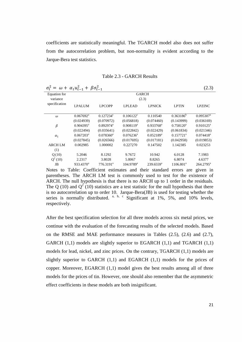
21

coefficients are statistically meaningful. The TGARCH model also does not suffer

from the autocorrelation problem, but non-normality is evident according to the

Jarque-Bera test statistics.

Table 2.3 - GARCH Results

(2.3)

Equation for

variance

specification

GARCH

(2.3)

LPALUM LPCOPP LPLEAD LPNICK LPTIN LPZINC

0.067692a

(0.024939)

0.127234c

(0.070972)

0.106122c

(0.056818)

0.110540

(0.074460)

0.363186b

(0.143999)

0.095307a

(0.036169)

0.904395a

(0.022494)

0.892974a

(0.035641)

0.908119a

(0.022842)

0.933768a

(0.022429)

0.758120a

(0.061834)

0.910125a

(0.021346)

0.067203a

(0.027845)

0.078360a

(0.026566)

0.076236a

(0.017695)

0.052189a

(0.017181)

0.157721a

(0.042958)

0.074418a

(0.019853)

ARCH LM

(1)

0.002985 1.000002 0.227270 0.147502 1.142385 0.023253

Q (10) 5.2046 8.1292 9.7672 10.942 6.0128 7.1983

Q2 (10) 2.2317 3.8028 5.8067 8.8265 6.8074 4.6377

JB 933.4370a 776.3191a 104.9789a 239.6559a 1106.801a 264.2795a

Notes to Table: Coefficient estimates and their standard errors are given in

parentheses. The ARCH LM test is commonly used to test for the existence of

ARCH. The null hypothesis is that there is no ARCH up to 1 order in the residuals.

The Q (10) and Q2 (10) statistics are a test statistic for the null hypothesis that there

is no autocorrelation up to order 10. Jarque-Bera(JB) is used for testing whether the

series is normally distributed. a, b, c Significant at 1%, 5%, and 10% levels,

respectively.

After the best specification selection for all three models across six metal prices, we

continue with the evaluation of the forecasting results of the selected models. Based

on the RMSE and MAE performance measures in Tables (2.5), (2.6) and (2.7),

GARCH (1,1) models are slightly superior to EGARCH (1,1) and TGARCH (1,1)

models for lead, nickel, and zinc prices. On the contrary, TGARCH (1,1) models are

slightly superior to GARCH (1,1) and EGARCH (1,1) models for the prices of

copper. Moreover, EGARCH (1,1) model gives the best results among all of three

models for the prices of tin. However, one should also remember that the asymmetric

effect coefficients in these models are both insignificant.

22

Table 2.4 - TGARCH Results

(2.4)

Equation for

variance

specification

TGARCH

(2.4)

LPALUM LPCOPP LPLEAD LPNICK LPTIN LPZINC

0.038165a

(0.013858)

0.120301c

(0.067481)

0.088879c

(0.053258)

0.107428

(0.073826)

0.432439a

(0.162062)

0.076209b

(0.030341)

0.919714a

(0.017411)

0.898546a

(0.035499)

0.915094a

(0.021898)

0.934275a

(0.022255)

0.728974a

(0.069925)

0.919886a

(0.020317)

-0.066756c

(0.038974)

0.001037

(0.039386)

-0.013496

(0.027498)

-0.004446

(0.028711)

0.085020

(0.087689)

-0.022893

(0.033575)

0.103946a

(0.031908)

0.073639c

(0.038227)

0.079685a

(0.026962)

0.054474b

(0.027055)

0.124323c

(0.067000)

0.081126b

(0.033583)

ARCH LM

(1)

0.000822 0.903491 0.336187 0.149492 0.787501 0.000829

Q (10) 5.6734 8.2721 9.7590 11.031 6.0691 7.5620

Q2 (10) 1.7591 3.6499 5.8695 8.6216 6.4211 4.0504

JB 642.1407a 791.0539a 108.2352a 234.6295a 1014.128a 276.9781a

Notes to Table: Coefficient estimates and their standard errors are given in

parentheses. The ARCH LM test is commonly used to test for the existence of

ARCH. The null hypothesis is that there is no ARCH up to 1 order in the residuals.

The Q (10) and Q2 (10) statistics are a test statistic for the null hypothesis that there

is no autocorrelation up to order 10. Jarque-Bera(JB) is used for testing whether the

series is normally distributed. a, b, c Significant at 1%, 5%, and 10% levels,

respectively.

Also the interpretation of MAPE results confirms the RMSE and MAE results (see

Tables (2.5), (2.6) and (2.7),) that GARCH (1,1) model results in a slightly better fit

than EGARCH (1,1) models for aluminum, lead, nickel, and zinc data. TGARCH

(1,1) model gives better results than EGARCH (1,1) and GARCH (1,1) models for

copper prices and EGARCH (1,1) gives a slightly better fit than GARCH (1,1) and

TGARCH (1,1) for tin prices when we look at the RMSE, MAE and MAPE results.

However, Theil inequality coefficient gives slightly conflicting results with other

three forecasting error statistics for all six data sets. Namely, according to Theil

inequality coefficient estimates TGARCH (1,1) model result in a better fit than

EGARCH (1,1) and GARCH (1,1) models for aluminum, lead, nickel, and zinc data

sets and GARCH (1,1) model result in a better fit than EGARCH (1,1) and

TGARCH (1,1) models for copper and tin data sets (see Tables (2.5), (2.6) and

23

(2.7)). Regardless of the model used, best forecast results are observed for tin among

the six metals studied.

Table 2.5 - EGARCH Forecast Statistics

(2.1)

Equation for

variance

specification

EGARCH

(2.1)

LPALUM LPCOPP LPLEAD LPNICK LPTIN LPZINC

RMSE 1.457008 2.068801 2.400428 2.639875 1.974897 2.251417

MAE 1.060954 1.436628 1.752658 1.914785 1.346196 1.633354

MAPE 0.954044 1.008427 0.93979 0.949081 0.904089 0.958337

TIC 0.029662 0.040594 0.050179 0.00598 0.026662 0.047784

Table 2.6 - GARCH Forecast Statistics

(2.3)

Equation for

variance

specification

GARCH

(2.3)

LPALUM LPCOPP LPLEAD LPNICK LPTIN LPZINC

RMSE 1.456375 2.068339 2.400340 2.639791 1.991592 2.249464

MAE 1.059823 1.436630 1.752576 1.913982 1.365957 1.631546

MAPE 0.947852 1.005874 0.938925 0.945501 0.947722 0.94753

TIC 0.005611 0.039218 0.048909 0.000668 0.09114 0.034492

Table 2.7 - TGARCH Forecast Statistics

(2.4)

Equation for

variance

specification

TGARCH

(2.4)

LPALUM LPCOPP LPLEAD LPNICK LPTIN LPZINC

RMSE 1.456373 2.068321 2.400465 2.639804 1.992378 2.249785

MAE 1.060286 1.436610 1.752690 1.914169 1.366440 1.631868

MAPE 0.951904 1.004915 0.940132 0.946334 0.946178 0.950101

TIC 0.023491 0.038708 0.05068 0.001911 0.089828 0.038328

24

2.5. Summary and Conclusions

In this study the six non-ferrous metals’ prices are modeled using nonlinear

autoregressive conditional heteroscedasticity models. We discover that the six prices

are governed by the conditional heteroscedasticity effects. Therefore, appropriate

models for these prices can be found within the GARCH family. We utilize the

GARCH, TGARCH and EGARCH models for all six prices in this research. Then

we compare the forecasting accuracy of the three models according to several

statistical criteria. We find that in general all three models show similar performance

in forecasting the prices of the six metals. However, the GARCH model performs

slightly better than the EGARCH and TGARCH models according to several criteria

for lead, nickel, and zinc metals. The MAE and MAPE choose the GARCH model,

whereas the RMSE and TIC choose the TGARCH model for aluminum prices. For

tin prices, the EGARCH model outperforms the GARCH and TGARCH models

according to several criteria. As for the copper prices, TGARCH seems to be the

most appropriate model. Since the GARCH model is more parsimonious and the

asymmetric effect coefficients in TGARCH and EGARCH models are insignificant,

we recommend the utilization of the GARCH model for forecasting the prices of all

six metal prices. The similar performances of the three models with respect to

statistical criteria do not necessarily imply that one of them will outperform the

others in practice. Therefore, further research would be beneficial in understanding

whether investors may profitably benefit from improved forecast accuracy depending

on several trading strategies.

25

CHAPTER III

VOLATILITY SPILLOVER FROM WORLD OIL MARKET TO NON-

FERROUS METAL MARKETS

3.1. Introduction

Changes in the oil price affect most sectors of most economies at various degrees.

Recent research has shown that commodity prices of all kinds rise and fall in unison.

Crude oil prices affect the prices of other commodities in a number of ways. Such

co-movements are typically attributed to common macroeconomic shocks on world

commodity markets, and complementarity or substitutability in the production or

consumption of related commodities. For instance, some metals such as aluminum

have to go through an energy-intensive primary processing stage. Pindyck and

Rotemberg (1990) find that the prices of a group of unrelated commodities had a

tendency to move together, even after accounting for the effects of common

macroeconomic variables. This co-movement and its explanations may be more

relevant to strategic commodities such as oil, gold, silver and copper which have

varying but important degrees of industrial usages and influences. This part focuses

on the pass-through of crude oil price changes to the prices of six internationally

traded non-ferrous metals.

Policy makers are mostly concerned about the short run and the long run impacts of

the recent rise and subsequent fall in world oil prices on the macroeconomy. On the

other hand, main issues of the traders are that whether these impacts are permanent

or temporary and how the non-ferrous metal returns will respond to oil shocks. Oil

price changes are generally found to have significant effects both on the economy

and financial markets. Several studies have examined the relationship between oil

prices and commodity prices, but a small number of studies focus on the impact of

oil shocks on non-ferrous markets, where academicians and practitioners alike have

26

been trying to understand the dynamic links between world oil prices and non-

ferrous metal returns.

The constant variance assumption is violated in financial time series, which means

periods of high volatility followed by periods of low volatility. The multivariate

GARCH models are the most appropriate method to deal with this violation.

McMillan and Speight (2001) state that the non-linear models have been the most

commonly used tools in modeling and forecasting volatility of returns in the short

run, but they may fail to capture the long run dynamics. This study is related to the

literature on the impact of oil price changes on commodity prices; however, it is

differentiated from the rest of the literature by examining the impact of fluctuations

of oil prices on non-ferrous metal returns as well as volatility spillovers. The stocks

of companies operating in metal markets are more sensitive to world oil price

changes.

In finance, there exists a wide area for the application of MGARCH models. An

illustrative list of some typical applications can be given by introducing the model of

the changing variance structure in an exchange rate regime (Bollerslev, 1990), the

optimal debt portfolio calculation in multiple currencies (Kroner and Claessens,

1991), the multiperiod hedge ratios evaluation of currency futures (Lien and Luo,

1994), the international transmission examination of stock returns and volatility

(Karolyi, 1995) and the optimal hedge ratio estimation for stock index futures (Park

and Switzer, 1995). However, we employ a multivariate GARCH model to

simultaneously estimate the appropriate residuals using daily returns from December

12, 2003 to December 15, 2008. Examination of temporal relationships through the

creation of large models with many lags is allowed when the powerful time series

techniques are introduced. In the literature the Granger causality tests are referred to

interpret the results as well as impulse response and variance decomposition

analyses, because of the problems in the interpretation of lagged variable

coefficients. An example for the interpretation of results can be given as; if lags of a

variable X improve the interpretation of another variable Y, then we can said that X

27

Granger causes Y. In the relevant literature of the oil price-commodity prices,

everybody believes that fluctuations in oil price changes affect the prices of other

commodities, but not vice versa, especially in minor commodity markets in relation

to the vital commodity markets. This theoretical belief does not always match with

the experimental results. Several reasons may exist ranging from the methodology

related problems to the commodity market characteristics. Reason for the absence of

a causal link between oil price and commodity prices is that there may be a dynamic

link between the variables themselves as well as the variances of the variables.

Hence, one should focus not only on mean, but also variance spillovers in order to

fully examine the dynamic links between oil and metal returns.

The chapter is organized as follows. In the next section a brief review of literature

that is related to the study is given. Section 3 discusses the data used in the study and

the methodology applied in the study. Section 4 presents empirical results while

section 5 concludes the chapter.

3.2. Literature Review

Here we first summarize GARCH models mainly used in modeling stock market

prices and volatilities as well as currency markets. Then we review studies that focus

on commodity prices, especially oil and metal prices. Please note that a bulk of the

literature has been reviewed in the first part of the thesis, therefore we do not delve

too deep into the literature in this part to avoid overlaps.

The survey paper of Bera and Higgins (1993) provide an account of some of the

important developments in the autoregressive conditional heteroscedasticity (ARCH)

model since it is introduced by Engle (1982) in his seminal paper. More and more

features of the real world are accommodated by generalized ARCH models. A

comprehensive treatment of many of the extensions of the original ARCH model is

provided in this paper. Moreover, estimation and testing for ARCH models are

discussed and note that these models lead to some interesting and unique problems.

28

Structural change, different kinds of nonlinearities, cointegration and finite sample

properties of estimators and test statistics are the problems that being investigated. In

this survey paper, they provide a brief account of these problems. The ARCH models

offer a more adaptive framework for nonlinear dynamic characteristics problem of

the financial time series than the classical ARMA models because of its limitations.

Gourieroux (1997) survey the recent work in this area from the perspective of

statistical theory, financial models, and applications and will be of interest to

theorists and practitioners.

Bollerslev, Chou and Kroner (1992) survey several research papers on the

methodology and applications of GARCH and MGARCH models that they consider

to be the most important and promising in the formulation of ARCH-type models.

This overview of the extensive ARCH literature serves as a catalyst in fostering

further research in this important area. The basic framework for a multivariate

generalized autoregressive conditional heteroscedasticity model is provided by

Bollerslev, Engle and Wooldridge (1988). The univariate case of the GARCH

representation is extended in to the vectorized conditional-variance matrix. They

estimate a MGARCH process for returns to bills, bonds, and stocks where the

expected return is proportional to the conditional covariance of each return with that

of a fully diversified or market portfolio. The main result of their paper is that the

conditional covariances are quite variable over time. Moreover, the implied betas are

also time-varying and forecastable. Engle and Kroner (1995) extend Engle's (1982)

ARCH model and Bollerslev's (1986) GARCH model to a multivariate setting by

presenting theoretical results on the formulation and estimation of multivariate

generalized ARCH models within simultaneous equations systems. For the sake of

parameterization of the multivariate process, a new formulation is proposed (BEKK)

and compared with the existing parameterization of the multivariate ARCH process,

the (VECH). Bauwens, Laurent and Rombouts (2006) review the multivariate

GARCH models which are increasingly used in applied financial econometrics.

According to them, providing a realistic but parsimonious specification of the

variance matrix ensuring its positivity is the crucial point in MGARCH modeling.

29

There is a trade-off between flexibility and parsimony. A lot of parameters are

needed for flexible BEKK. On the other hand, restrictive diagonal VEC and BEKK

models are much more parsimonious.

Another step forward in methodological development is allowing the conditional

correlations to vary through time. The theoretical and empirical properties of

Dynamic Conditional Correlation (DCC) Multivariate GARCH are developed by

Engle and Sheppard (2001). S&P 500 Sector Indices and Dow Jones Industrial

Average stocks are used to estimate the conditional covariance of up to 100 assets

using and to conduct specification tests of the estimator using an industry standard

benchmark for volatility models. However, we limit ourselves to MGARCH models

and assume constant conditional correlations, so that our results are comparable to

studies that employ the same methodology in different commodity markets.

In their article, King and Wadhwani (1990) investigate the outcome of rational

attempts to use imperfect information about the events in order to examine a rational

expectations price equilibrium and model contagion between markets. A contagion

model is constructed to explain why all stock markets fell together despite widely

differing economic circumstances. Market prices reveal all relevant information to

agents in models of rational expectations equilibrium with asymmetric information,

provided that there is a relatively simple information structure. They show that

covariances are related to volatility with high-frequency data. An implication of this

result is that an increase in volatility could be self-reinforcing and persist for longer

than would otherwise be the case. As volatility declines, market links become

weaker, and price changes are less closely tied together.

Bollerslev (1990) propose a simple multivariate conditional heteroscedastic time

series model. The model has constant conditional correlations, but time varying

conditional variances and covariances. The estimation and inference procedures are

greatly simplified with the help of this structure. The parameterization proposed here

with constant conditional correlations but time varying conditional covariances

30

represents a major increase in terms of computational simplicity when compared to

Bollerslev, Engle and Wooldridge (1988)’s the linear diagonal GARCH model,

Diebold and Nerlove (1989)’s the latent factor ARCH model, or Engle, Ng, and

Rothschild (1990)’s the factor GARCH model. Finally, the various ARCH and

GARCH parameterizations suggested in the literature represent nothing but a

convenient statistical tool for summarizing the time series dependence observed in

the data.

A multivariate Generalized Autoregressive Conditional Heteroscedasticity (GARCH)

model is used to estimate a sequence of optimal dynamic hedging portfolios, since

the model of Kroner and Claessens (1991) permits the second moments to change

through time. Actual model shows that the currency composition of a country's

external debt can serve as a hedging instrument against changes in exchange rates

and commodity prices. They apply it to Indonesia to illustrate the usefulness of the

technique. As expected, this application shows that Indonesia's optimal debt portfolio

consists of a much larger proportion of US dollars and a much smaller proportion of

Japanese yen than they have in their current debt portfolio.

In their article, Engle and Susmel (1993) investigate whether two international stock

markets share the same volatility process by using the advantage of the time-varying

structure of stock-returns variances. A recent test which is developed by Engle and

Kozicki is used to assess the validity of a one-factor autoregressive conditional

heteroscedasticity model. Main result of this paper is that some international stock

markets have the same time-varying volatility.

Lien and Luo (1994) use a basic bivariate GARCH model for multiperiod hedge ratio

estimates. The optimal multiperiod hedge ratio is derived prior to the introduction of

conditional heteroscedasticity into the joint price process. An error correction model

describes the mean process while the GARCH specification is applied to model the

conditional heteroscedasticity. This model is applied, in order to empirically

determine the hedge ratios major foreign exchange markets. For each case, GARCH

31

hedge ratios perform a little better than three alternative hedge strategies (no hedge,

constant hedge and error correction hedge).

Karolyi (1995) use a bivariate generalized autoregressive conditional heteroscedastic

(GARCH) model to examine the dynamic relationship between daily stock-market

returns and return volatilities of the U.S. and Canadian. Two tests are conducted with

this model. First test is how rapidly stock-return innovations originating in the U.S.

and Canadian markets transmit to the other market and second one is how rapidly the

volatility of these innovations transmits to the other market by simulating the

impulse responses of the estimated bivariate GARCH model. The relationships

between stock-price movements in the U.S. and Canadian markets are confirmed by

the test results which show that the bivariate GARCH model is a reasonable

representation. More precisely, tests using multivariate GARCH models indicate that

the effects of shocks are smaller and less persistent than those measured with

traditional vector autoregressive (VAR) models.

Huang, Masulis and Stoll (1996) use a multivariate vector autoregressive (VAR)

approach to examine the contemporaneous and lead-lag correlations between daily

returns of oil futures contracts and stock returns which answer the general question

of the information transmission mechanism linking oil futures with stock prices. One

of the many possible scenarios is that the relevant information affecting each of these

markets is informationally segmented from the other, oil futures prices and stock

prices will be unrelated. Dynamic interactions among price changes of different

financial instruments are easily examined by the highly flexible framework of the

VAR representation. The conclusions from the VAR approach are oil futures returns

are not correlated with stock market returns. In fact, the lack of correlation suggests

that oil futures, like other futures contracts that also appear to have little correlation

with stocks, are a good vehicle for diversifying stock portfolios (Huang, Masulis and

Stoll, 1996).

32

A simple model of speculative trading is developed by Fleming, Kirby and Ostdiek

(1998) to examine the nature of volatility linkages in an economy which is based on

the relation between volatility and information flow in multiple securities markets. In

speculative trading, traders’ current expectations and risk tolerances influence the

trader’s positions in one or more futures contracts. Market linkages are generated in

two ways by information under the model. First one is that the information is

common across markets and second one is that there is an information spillover

between markets). According to Fleming Kirby and Ostdiek (1998), ―The model

predicts strong volatility linkages in markets where the hedging benefits are large

and the hedging costs are small. We use a stochastic volatility representation of the

model to estimate the volatility linkages for three futures markets where we expect

both common information and information spillover to be important: the stock, bond,

and money markets.‖

Pan and Hsueh (1998) employ a two-step GARCH approach to examine the nature of

transmission of stock returns and volatility between the U.S. and Japanese stock

markets by using stock index futures prices on the S&P 500 and Nikkei 225 stock

indexes in order to obtain more robust results. Results show that there are

unidirectional contemporaneous return and volatility spillovers from the U.S. to

Japan. Another interpretation of the results is that there are no significant lagged

spillover effects in both returns and volatility from the Osaka market to the Chicago

market, while a significant lagged volatility spillover is observed from the U.S. to

Japan. Hafner and Herwartz (1998) use a multivariate GARCH framework to give

empirical evidence of time-varying market price of risk for the German stock market.

De Santis and Gerard (1998) use a parsimonious multivariate GARCH process to test

the conditional version of an International Capital Asset Pricing Model (ICAPM).

They find strong support for a specification of the ICAPM that includes both market

risk and foreign exchange risk, assuming that the prices are allowed to change over

time. Results show that if both the market and currency risk components are

incorporated into the model, there will be no need to use the additional information

variables to explain the cross-section and the dynamics of expected returns.

33

Sadorsky (1999) investigates the impact that oil price shocks may have on stock

market returns by using monthly data. Results from a VAR suggest that changes in

economic activity have little impact on oil prices but changes in oil prices impact

economic activity and the results of impulse response functions suggest that positive

shocks to oil prices depress real stock returns while shocks to real stock returns have

positive impacts on interest rates and industrial production.

Kearney and Patton (2000) contribute to the MGARCH modeling and exchange rate

volatility transmission literature by presenting a series of 3-, 4- and 5-variable

multivariate GARCH models to examine how exchange rate volatility is transmitted

with the EMS exchange rate system. They argue that alternative specifications

should be examined to clarify the robustness of results.

Kim (2000) uses a multivariate GARCH-M model to analyze the relation of

exchange rate volatility and output volatility. Source decomposition of observed

volatility of output into domestic factors, foreign factors and exchange rate

movements and also extraction of the expected volatility from the total volatility is

easily accomplished by the multivariate GARCH-M modeling. According to the

results, Japanese economy is insulated itself from foreign shocks with the help of the

floating exchange rate regime.

Tse and Tsui (2000) adopt the VECH representation to propose a new MGARCH

model with time-varying correlations. However, the conditional variances and

conditional correlations are the variables of interest. Their new model satisfies the

positive-definite condition as found in the constant-correlation and BEKK models

while retaining the intuition and interpretation of the univariate GARCH model.

In addition to stock market and currency market applications, the GARCH models

are also frequently used in the recent literature on commodity prices, especially the

oil prices. The interest ranges from the link between different energy prices to oil

spills to other commodity and financial markets.

34

There are several recent studies that analyze the dynamics of metal prices along with

oil. For example, Sari et al. (2010), Soytas et al. (2009), and Hammoudeh et al.

(2009) focus on the link between precious metals with various other variables, like

oil price and the exchange rate. These studies put forth the importance of

investigating the dynamics of metal prices. Since they do not focus on volatility

transmissions we do not discuss them in too much detail here.

Ewing, Malik and Ozfidan (2002) use daily returns data to examine the transmission

of volatility between the oil and natural gas sectors changes over time and across

markets. . The univariate and bivariate time-series properties of oil and natural gas

index returns are empirically examined by robust methodology in which the changes

in volatility in one market may spill over to the other market is allowed and non-

linearity in the variance of each series can easily be examined. Results of the study

show that returns exhibit time-varying volatility which implies volatility in natural

gas returns is more persistent than volatility in oil returns.

Hammoudeh, Dibooglu and Aleisa (2004) employ unit root tests, cointegration tests,

error-correction models with day effects, and univariate and multivariate

ARCH/GARCH models with day and oil spillover effects to examine the intra- and

interlinks for two U.S. markets of oil prices and S&P oil sector stock indices. In this

study, the multivariate GARCH model helps to capture simultaneous volatility

interactions. Moreover, MGARCH model shows that the transmission of volatility

between prices, something that was not revealed by the univariate GARCH model.

Bhar and Hamori (2005) use a recent econometric methodology to analyze causal

relationship between crude oil futures return and the trading volume using daily data

over a ten-year period. The two-step procedure developed by Cheung and Ng (1996)

is used and they find only causality at higher order lags running from return to

volume in the mean as well as in conditional variance. There exist several conflicts

with earlier studies in this area. We utilize the same methodology in this study.

35

Eckner (2006) introduces a model for asset returns that incorporates joint

heteroscedasticity as well as time varying correlations which is suitable for capturing

the dynamics of multivariate return time series. The empirical results give an

explanation why the volatility smile in index options tends to be more pronounced

than in individual stocks options.

Malik and Hammoudeh (2007) estimate the mean and conditional variance of daily

returns in the oil, US and Gulf equity markets at the same time by using the BEKK

specification of the multivariate GARCH model. The main reason behind using the

BEKK is that it does not impose the restriction of constant correlation among

variables over time. They examine the volatility and shock transmission among US

equity market, global crude oil market, and equity markets of major oil rich Gulf

countries since shocks can spillover from one country to another. The results show

significant volatility transmission among US equity market, global crude oil market,

and equity markets of major oil rich Gulf countries. Additionally, these results are

important for building accurate asset pricing models and forecasting future volatility

in equity and oil markets.

Inagaki (2007) employ the residual cross-correlation approach to investigate

volatility spillover between the British pound and the euro. They believe that the

causality in variance approach is useful for analyzing exchange rates that often

exhibit conditional heteroscedasticity. Since it does not involve simultaneous

modeling which makes it is easier to implement than the multivariate method. Their

findings suggest that the euro volatility has a one-sided impact on the British pound

volatility and they conclude that the euro is the most influential European currency.

In the review paper of Silvennoinen and Terasvirta (2008) a number of multivariate

GARCH models and its specifications are surveyed. Using the original VEC model

is obviously very tedious because of too many parameters, so finding parsimonious

alternatives is the main focus of this research. Two alternatives are generated. First,

some restrictions are imposed on the parameters of the VEC model to create new

36

models, such as the BEKK model and the factor models. Second, modeling

conditional covariance through conditional variances and correlations is another idea.

Several new models are generated, and conditional correlation model family seems

to become quite popular.

In order to extract information for risk prediction Chow and Fung (2008) use a

MGARCH structure to offer a quantitative approach to analyzing possible

associations of stock price changes and variations in innovative activities. Results

show that the model can pick up the correlation between the two variables and aid in

producing accurate Value-at-Risk estimates. The statistical evidence is confirmed by

the model comparison exercises which suggest that the assumption of MGARCH

(1,1) is sufficient for this type of study.

3.3. Data & Methodology

3.3.1. Data

We use daily data on the mean three-month futures prices of six commonly traded

non-ferrous metals (aluminum, copper, lead, nickel, tin, and zinc), and spot oil price

for the period December 12, 2003 – December 15, 20081. All three-month futures

prices are sourced from London Metal Exchange (LME) and these prices are given in

US dollars per ton. The ―Dated Brent‖ Spot Price reflects the average price of

―Brent-Forties-Oseberg-Ekofisk‖ (BFOE) cargoes loading 10-21 days forward and

given in US dollars per barrel. The total observations for each data set are 1305. The

natural logarithms of all data are arranged in 5 day weeks and all holidays are

removed.

In non-ferrous metal markets, futures price is combination of spot price, interest and

storage costs. In some sense, the futures price is above spot because by buying

1 We have chosen the start date so as to move as far away from the effects of 9/11, this allowed us

to retain more than 1300 observations.

37

forward the purchaser avoids the finance and storage cost. However, we use the spot

oil prices instead of futures, since oil prices are very volatile. But much of this

volatility seems to be reflected in short-term, transitory factors that may have little or

no influence on the price in the long run. Moreover, consistent with the practice in

the finance literature, there really is no "true" spot market for oil, in the sense of that

there is a "true" spot market for stock or other financial assets. A "true" spot market

requires the actual physical transfer of the goods, to the purchaser, directly at the

time of purchase. When we refer to "futures" price for crude oil, it includes spot

price, interest, storage costs and scarcity/prompt/convenience premium. In that case

using spot oil price instead of futures is more convenient for our study.

3.3.2. Methodology

The first step in the procedure is assuring the stationarity of each price series by

using the unit root tests. The unit root test procedures are already summarized in

Chapter 2 of this thesis (see page 14). Then, the multivariate GARCH process is

modeled to analyze the price spillovers from oil market to non-ferrous metal markets.

In order to start modeling, the specification of the mean equation should be

identified. The following mean equation is selected and estimated for each price

series:

(3.1)

where, is a vector of daily prices between and , the vector of

random errors is the error term for the price on index at time . The vector

, represents long-term drift coefficient. A variant of the multivariate GARCH model

is used because the possibility of volatility transmission among two markets is

analyzed in addition to volatility persistence analysis within each market.

In the literature, several MGARCH parameterizations are presented, such as vector

ARCH model (VEC, initially due to Bollerslev, Engle and Wooldridge, 1988),

diagonal VEC model (DVEC), the BEKK model (named after Baba, Engle, Kraft

38

and Kroner), Constant Conditional Correlation Model (CCC, Bollerslev, 1990),

Dynamic Conditional Correlation Model (DCC models of Tse and Tsui (2002) and

Engle (2002)). In this study, the BEKK model is employed because the estimated

covariance matrix of equations will be positive semi-definite since it depends on the

squares and cross products of error term and volatility for each market. Namely, this

model ensures the non-negative estimated variances, and, at the same time does not

require estimation of a large number of parameters.

The BEKK parameterization for the multivariate GARCH (1,1) model can be given

as:

(3.2)

where, is the matrix of conditional variance, is a symmetric matrix

with constant parameters , is a diagonal matrix of parameters

which measures the extent of deviations from the mean (i.e., the ARCH term), and

is also a diagonal matrix of parameters which indicates the persistence in

conditional volatility between market and market (i.e., the GARCH term). In other

words, the effects of shocks or volatility can be captured by .

In our bivariate case, the conditional variance for each equation can be written as:

(3.3)

(3.4)

and the conditional covariance can be written as:

(3.5)

39

The above equations show the transmission pattern of shocks and volatility between

markets and over time. In this study, six models with two variables are estimated to

predict current period’s variance by forming a weighted average of a long term

average (the constant), volatility condition in the previous period (the ARCH term),

and the last period’s forecasted variance (the GARCH term).

Next the Granger causality-in-variance approach based on squares of the

standardized residuals is considered which is developed by Cheung and Ng (1996).

The standardized residuals,

, used in the sample residual cross-

correlation function are obtained from MGARCH models, where represent the

stationary series and is the conditional variance. The squares of the two

standardized residuals, , are obtained for the Granger causality-in-variance and

used to derive the sample residual cross-correlation functions between them. The

sample residual cross-correlation functions between two squared standardized

residuals can be written as;

(3.6)

where is the sample cross covariance function which can be given as

(3.7)

where T is the sample size. The cross-correlation, , at different lags has

asymptotic normal distribution in large samples and under no causality hypothesis

and regularity conditions.

40

3.4. Empirical Results

First we have to investigate the time series properties of the series. Descriptive

statistics for the corresponding return series are presented in Table (3.1). Price return

volatility is measured by the standard deviation, which is highest in nickel, followed

by lead, zinc, copper, tin, oil and aluminum. In terms of skewness, all of the data

series are skewed to the left. According to Malik and Hammoudeh (2007), investors

in positively skewed markets would be willing to accept smaller returns than

investors in negatively skewed markets when the market is up, provided that the

losses are not too serious when the market is down. All series exhibit excessive

kurtosis, a fairly common occurrence in high frequency financial time series data.

The null hypothesis of normality of The Jarque–Bera statistics are rejected for all

return series.

Summary of the results of the unit root tests are given in Table (3.2). ADF, DF–GLS,

and PP critical values are sourced from MacKinnon (1991). KPSS critical values are

from Kwiatkowski, Phillips, Schmidt, and Shin (1992) and MZα critical values are

from Ng and Perron (2001). Elliot, Rothenberg, and Stock (1996) gives the critical

values of ERS. Although the results seems to maintain a conflict between the tests, in

general all six non-ferrous metal prices and oil price are stationary in levels which

means that they are stationary in levels.

Table 3.1 – Descriptive statistics for log returns

LPALUM LPCOPP LPLEAD LPNICK LPTIN LPZINC LPOIL Mean -0.003607 0.028838 0.031660 -0.018965 0.051181 0.006114 0.031026

Median 0.000000 0.000000 0.000000 0.000000 0.000000 0.000000 0.118613

Maximum 4.826176 11.35608 11.18281 15.63461 12.62937 8.773891 8.016617

Minimum -8.613185 -14.96521 -10.87128 -18.16888 -12.36140 -11.74037 -9.205643

Std. Dev. 1.484822 2.132294 2.443550 2.688935 2.038836 2.270085 1.765930

Skewness -0.643612 -0.557645 -0.395643 -0.190390 -0.496107 -0.524839 -0.506974

Kurtosis 5.712426 8.104604 5.146865 6.354868 8.951577 5.354081 5.430359

Jarque-

Bera

489.7714a 1483.346a 284.4438a 619.4071a 1978.046a 360.9646a 376.7872a

Notes to table: a, b, c Significant at 1%, 5%, and 10% levels, respectively.

41

Stationarity of the series is tested so that it is understood that they do not contain unit

roots as can be observed from Table (3.2). According to the test results with different

specifications the series employed do not contain unit roots.

Table 3.2 – Unit root test results

LEVEL ADF DF–GLS PP KPSS ERS NP (MZα)

Inte

rcep

t

LPOIL -30.24967a

(0)

-30.04821a

(0)

-30.40994a

(9)

0.573191b

(11)

0.102239

(0)

-631.175a

(9)

LPALUM -37.93146a

(0)

-8.462779a

(7)

-37.93148a

(1)

0.730881b

(1)

0.117576

(0)

-60.7828a

(7)

LPCOPP -39.77678a

(0)

-3.008679a

(11)

-39.65863a

(9)

1.007609a

(7)

0.103740

(0)

-5.19327

(11)

LPLEAD -35.06245a

(0)

-2.019194b

(18)

-35.08604a

(3)

0.468279b

(4)

0.071697

(0)

-3.58724

(18)

LPNICK -36.83380a

(0)

-1.935740c

(10)

-36.83006a

(8)

0.486622b

(8)

0.190515

(0)

-4.40567

(10)

LPTIN -35.02973a

(0)

-4.850927a

(9)

-35.01093a

(5) 0.228858

(4)

0.111333

(0)

-18.8587a

(9)

LPZINC -37.39598a

(0)

-8.783922a

(7)

-37.39501a

(2)

0.965631

(4)

0.061405

(0)

-70.8203a

(7)

Tre

nd

& I

nte

rcep

t

LPOIL -30.39388a

(0)

-12.80274a

(3)

-30.43469a

(7)

0.177249b

(10)

0.261593

(0)

-240.527a

(3)

LPALUM -38.10719a

(0)

-7.882113a

(7)

-38.10845a

(4)

0.211725b

(6)

0.233878

(0)

-52.1181a

(7)

LPCOPP -40.03118a

(0)

-5.152675a

(11)

-40.04963a

(6)

0.235424a

(2)

0.186908

(0)

-13.3098

(11)

LPLEAD -35.14776a

(0)

-20.96489a

(1)

-35.14776a

(0)

0.219265a

(1)

0.156521

(0)

-494.132a

(1)

LPNICK -36.90949a

(0)

-3.692934a

(10)

-36.90045a

(7)

0.202120

(7)

0.227075

(0)

-15.1391c

(10)

LPTIN -35.05110a

(0)

-6.727110a

(9)

-35.03616a

(6)

0.183636b

(5)

0.201831

(0)

-36.8733a

(9)

LPZINC -37.59474a

(0)

-36.36479a

(0)

-37.60362a

(6)

0.214173b

(8)

0.159675

(0)

-651.455a

(0)

Notes to table: Numbers in parentheses are the lag lengths. a, b, c

Significant at 1%,

5%, and 10% levels, respectively. All of the null hypotheses are unit root, except

KPSS; however, in KPSS the null is stationarity.

MGARCH models are commonly used to study the relationships between the

volatilities of multiple markets (Karolyi, 1995) and help to explain the one market

volatility is causing the other markets volatility. MGARCH models can also explain

whether the price volatility is transmitted to another price directly (conditional

variance) or indirectly (conditional covariances), or a shock within a market

increases another markets volatility. Estimated results for each variance equation of

the BEKK parameterization for the multivariate GARCH (1,1) model are given in

42

Table (3.3). Table (3.3) reports the results from the model using the price returns of

oil and one metal, subscripted by the numbers 1 and 2, respectively.

Table 3.3 – Results of the bivariate GARCH models

Independent

Variable

OIL

AL

UM

0.355684

(9.658486)

- 0.962877

(178.3832)

-

- 0.076758

(12.46019)

- 0.881465

(92.11086)

OIL

CO

PP

0.029700

(9.550352)

- 0.982916

(190.5847)

-

- 0.070944

(15.37148)

- 0.899451

(126.6809)

OIL

LE

AD

0.031407

(9.594076)

- 0.963297

(178.2159)

-

- 0.071866

(12.08336)

- 0.912461

(128.6587)

OIL

NIC

K

0.029364

(9.103366)

- 0.965190

(174.3155)

-

- 0.053134

(13.24763)

- 0.925517

(156.4269)

OIL

TIN

0.027503

(9.963412)

- 0.969110

(213.9894)

-

- 0.161599

(18.79795)

- 0.743537

(68.34661)

OIL

ZIN

C

0.028802

(9.502903)

- 0.966298

(185.7786)

-

- 0.072956

(13.71279)

- 0.908971

(133.8483)

Notes to table: denotes the conditional variance for the oil return series, and

is the conditional variance for the metal return series. t-values given in

parentheses. The multivariate GARCH model uses the BEKK parameterization.

Results of estimated mean equation and constants of each variance equation are not

reported for the sake of brevity.

The presence of autoregressive conditional heteroscedasticity in oil and metal price

couples is confirmed by the significance of the estimated parameters. Our results

show significant volatility transmission between the global oil markets and each of

the non-ferrous metal markets. Not surprisingly, in all of the models, metal prices are

directly positively affected by volatility from the oil market. Namely, all six non-

ferrous metal markets receive volatility from the oil market implying that financial

market participants of non-ferrous markets can potentially forecast the future

changes in each metal market by following developments in global oil market.

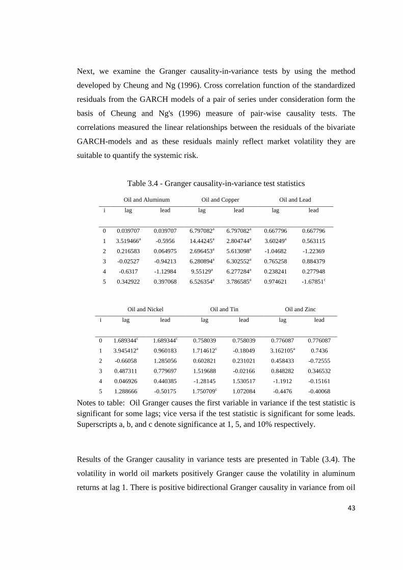
43

Next, we examine the Granger causality-in-variance tests by using the method

developed by Cheung and Ng (1996). Cross correlation function of the standardized

residuals from the GARCH models of a pair of series under consideration form the

basis of Cheung and Ng's (1996) measure of pair-wise causality tests. The

correlations measured the linear relationships between the residuals of the bivariate

GARCH-models and as these residuals mainly reflect market volatility they are

suitable to quantify the systemic risk.

Table 3.4 - Granger causality-in-variance test statistics

Oil and Aluminum Oil and Copper Oil and Lead

i lag lead lag lead lag lead

0 0.039707 0.039707 6.797082a 6.797082a 0.667796 0.667796

1 3.519466a -0.5956 14.44245a 2.804744a 3.60249a 0.563115

2 0.216583 0.064975 2.696453a 5.613098a -1.04682 -1.22369

3 -0.02527 -0.94213 6.280894a 6.302552a 0.765258 0.884379

4 -0.6317 -1.12984 9.55129a 6.277284a 0.238241 0.277948

5 0.342922 0.397068 6.526354a 3.786585a 0.974621 -1.67851c

Oil and Nickel Oil and Tin Oil and Zinc

i lag lead lag lead lag lead

0 1.689344c 1.689344c 0.758039 0.758039 0.776087 0.776087

1 3.945412a 0.960183 1.714612c -0.18049 3.162105a 0.7436

2 -0.66058 1.285056 0.602821 0.231021 0.458433 -0.72555

3 0.487311 0.779697 1.519688 -0.02166 0.848282 0.346532

4 0.046926 0.440385 -1.28145 1.530517 -1.1912 -0.15161

5 1.288666 -0.50175 1.750709c 1.072084 -0.4476 -0.40068

Notes to table: Oil Granger causes the first variable in variance if the test statistic is

significant for some lags; vice versa if the test statistic is significant for some leads.

Superscripts a, b, and c denote significance at 1, 5, and 10% respectively.

Results of the Granger causality in variance tests are presented in Table (3.4). The

volatility in world oil markets positively Granger cause the volatility in aluminum

returns at lag 1. There is positive bidirectional Granger causality in variance from oil

44

returns to the copper returns and vice versa at all lags. Oil volatility positively

Granger cause lead volatility at lag 2, with a positive feedback from lead volatility to

oil volatility at lag 5. The volatility in oil market positively Granger cause the

volatility in the nickel market at lags 0 and 1, while the volatility in nickel market

positively Granger cause the volatility in oil market at lag 0. There is positive

unidirectional Granger causality in variance from oil returns to the tin returns at lags

1 and 5. Positive Granger causality exists from oil volatility to zinc volatility at lag 1.

The volatility spillover results help to detect the causal relationship between world

oil prices and non-ferrous metal prices.

3.5. Summary and Conclusions

In this study the six non-ferrous metals’ prices and oil price are used to examine the

causal relationships between each non-ferrous metal and oil price by using bivariate

nonlinear autoregressive conditional heteroscedasticity models. In the first part of

this thesis, we discover that the prices of six non-ferrous metals are governed by the

conditional heteroscedasticity effects and according to this study oil price reflects the

same characteristics. Since the volatility in metal markets may be related to the

volatility in oil market, the multivariate GARCH model is used to form valid

residuals for the Granger causality in variance tests. The Granger causality in

variance tests is carried out by using the method developed by Cheung and Ng

(1996). Our results seem to be in line with the previous studies in that the crude oil

market volatility leads all non-ferrous metal markets. The result that there is

bidirectional causality in variance between oil and copper is not unusual, since this

metal is found to be a good indicator of macroeconomic developments. Because of

this feature, it has been referred to as Dr. Copper in the literature. In our study,

copper appears to be as important as oil. However, it would be interesting to check

whether copper prices and volatilities lead other metals as a future study.

45

REFERENCES

Agnolucci, P. (2009). Volatility in crude oil futures: A comparison of the predictive

ability of GARCH and implied volatility models. Energy Economics , 31, 316–321.

Allen, P. G., & Morzuch, B. J. (2006). Twenty-five years of progress, problems, and

conflicting evidence in econometric forecasting. What about the next 25 years?

International Journal of Forecasting, 22, 475– 492.

Asai, M., & McAleer, M. (2008). A Portfolio Index GARCH model. International

Journal of Forecasting, 24, 449–461.

Bauwens, L., Laurent, S. and Rombouts, J. V. K. (2006). Multivariate GARCH

Models: A Survey. Journal Of Applied Econometrics, 21, 79–109.

Bera, A. and Higgins, M. (1993). ARCH models: Properties, estimation and testing.

Journal of Economic Surveys, 7, 305– 365.

Bhar, R. and Hamori, S., (2005). Empirical Techniques in Finance. Springer, New

York.

Bollerslev, T. (1986). Generalized Autoregressive Conditional Heteroskedasticity.

Journal of Econometrics, 31 (3), 307-327.

Bollerslev, T. (1990). Modelling the coherence in short-run nominal exchange rates:

A multivariate generalized ARCH approach. Review of Economics and Statistics, 72,

498-505.

Bollerslev, T., Chou, R. Y. and Kroner, K. F. (1992). ARCH modeling in finance: A

review of the theory and empirical evidence. Journal of Econometrics, 52, 5 – 59.

Bollerslev, T., Engle, R. and Wooldridge, J. (1988). A capital asset pricing model

with time varying covariances. Journal of Political Economy, 96, 116-131.

Bowden, N., & Payne, J. E. (2008). Short term forecasting of electricity prices for

MISO hubs: Evidence from ARIMA-EGARCH models. Energy Economics , 30,

3186–3197.

Bozdogan, H. (2000). Akaike's Information Criterion and Recent Developments in

Information Complexity. Journal of Mathematical Psychology, 44, 62-91.

46

Cheung, Y. and Ng, L. K. (1996). A causality-in-variance test and its application to

financial market prices. Journal of Econometrics, 72, 33–48.

Chou, R. (1988). Volatility persistence and stock valuations: some empirical

evidence using GARCH. Journal of Applied Econometrics, 279-294.

Chow, W. W. And Fung, M. K. (2008). Volatility of stock price as predicted by

patent data: An MGARCH perspective. Journal of Empirical Finance, 15, 64–79.

De Gooijer, J. G., & Hyndman, R. J. (2006). 25 years of time series forecasting.

International Journal of Forecasting, 22, 443– 473.

De Santis, G. and Gerard, B. (1998). How big is the premium for currency risk?

Journal of Financial Economics, 49, 375–412.

Dickey, D., & Fuller, W. (1979). Distribution of the Estimators for Autoregressive

Time Series with a Unit Root. Journal of the American Statistical Association, 74,

427–431.

Diebold, FX and Nerlove, M. (1989). The dynamics of exchange rate volatility: a

multivariate latent factor ARCH model. Journal of Applied Econometrics, 4, 1–21.

Dooley, G., & Lenihan, H. (2005). An assessment of time series methods in metal

price forecasting. Resources Policy, 30, 208–217.

Eckner, A. (2006). A Multivariate Garch Model with Volatility Spill-Over and Time-

Varying Correlations. Working Paper.

Elliott, G., Rothenberg, T. J., & Stock, J. (1996). Efficient Tests for an

Autoregressive Unit Root. Econometrica, 64 (4), 813-836.

Engle, R. (2004). Risk and Volatility: Econometric Models and Financial Practice.

The American Economic Review , 94 (3), 405-420.

Engle, R. F. (1982). Autoregressive Conditional Heteroscedasticity with Estimates of

the Variance of United Kingdom Inflation. Econometrica, 50 (4), 987-1007.

Engle, R. F., & K, N. V. (1993). Measuring and Testing the Impact of News on

Volatility. The Journal of Finance , 48 (5), 1749-1778.

Engle, R.F. (2002). Dynamic conditional correlation—a simple class of multivariate

GARCH models. Journal of Business and Economic Statistics, 20, 339–350.

Engle, R.F. and Sheppard, K. (2001). Theoretical and empirical properties of

dynamic conditional correlation multivariate GARCH. Mimeo, UCSD.

47

Engle, R.F. and Susmel, R. (1993). Common Volatility in International Equity

Markets. Journal of Business and Economic Statistics, 11 (2), 167-176.

Engle, R.F., Ng, V. K. and Rothschild, M. (1990). Asset pricing with a factor-ARCH

covariance structure: empirical estimates for treasury bills. Journal of Econometrics,

45, 213–238.

Ewing, B. T., Malik, F. and Ozfidan, O. (2002). Volatility transmission in the oil

and natural gas markets, Energy Economics, 24(6), 525-538.

Figuerola-Ferretti, I., & Gilbert, C. L. (2008). Commonality in the LME Aluminum

and Copper Volatility Processes. The Journal of Futures Markets , 28 (10), 935–962.

Fleming, J., Kirby, C. and Ostdiek, B. (1998). Information and volatility linkages in

the stock, bond, and money markets. Journal of Financial Economics, 49 (1), 111-

137.

French, K. R., Schwert, G. W., & Stambaugh, R. F. (1987). Expected stock returns

and volatility. Journal of Financial Economics, 19, 3-30.

Gillian Dooley, H. L. (2005). An assessment of time series methods in metal price

forecasting. Resources Policy , 208–217.

Glosten, L. R., Jagannathan, R., & Runkle, D. E. (1993). On the Relation between

the Expected Value and the Volatility of the Nominal Excess Return on Stocks.

Journal of Finance , 48 (5), 1779-1801.

Gouriéroux, C. (1997). ARCH Models and Financial Applications, Springer Verlag.

Hafner, C. and Herwartz, H. (1998). Time-varying market price of risk in the CAPM.

Approaches, empirical evidence and implications. Finance, 19, 93–112.

Hamao, Y.R., Masulis, R.W. and Ng, V.K. (1991). The Effect of the 1987 Stock

Crash on International Financial Integration. Japanese Financial Market Research,

Elsevier, 483-502.

Hammoudeh, S., & Yuan, Y. (2008). Metal volatility in presence of oil and interest

rate shocks. Energy Economics, 30, 606–620.

Hammoudeh, S., Dibooglu, S. and Aleisa, E. (2004). Relationships among US Oil

Prices and Oil Industry Equity Indices. International Review of Economics and

Finance, 13 (3).

48

Hammoudeh, S., Sarı, R. and Ewing, B. T. (2009). Relationships among Strategic

Commodities and With Financial Variables. Contemporary Economic Policy, 27 (2),

251-264.

Hanke, J. E., & Reitsch, A. G. (1998). Business Forecasting. Upper Saddle River,

N.J.: Prentice Hall.

Hodge, B. J. (2003). Organization Theory: A Strategic Approach, 6th Edition.

Prentice Hall.

Huang, R., Masulis, R. and Stoll, H (1996), Energy Shocks and Financial Markets.

Journal of Futures Markets, 16 (1), 1-27.

Inagaki, K. (2007). Testing for volatility spillover between the British pound and the

euro. Research in International Business and Finance, 21(2), 161-17.

Karanasos, M., & Kim, J. (2003). Moments of the ARMA–EGARCH model.

Econometrics Journal , 6, 146–166.

Karolyi, G. A. (1995). A Multivariate GARCH Model of International

Transmissions of Stock Returns and Volatility: The Case of the United States and

Canada. Journal of Business & Economic Statistics, 13 (1), 11-25.

Kearney, C. and Patton, A.J. (2000). Multivariate GARCH modelling of exchange

rate volatility transmission in the European Monetary System. Financial Review, 41,

29–48.

Kim, J. (2000). The relationship between the monetary regime and output volatility:

a multivariate GARCH-M model of the Japanese experience, 1919–1996. Japan and

the World Economy, 12, 49–69.

King, M. A. and Wadhwani, S. (1990). Transmission of Volatility between Stock

Markets. The Review of Financial Studies, 3 (1), 5-33.

Kroner, K.F. and Claessens, S. (1991). Optimal dynamic hedging portfolios and the

currency composition of external debt. Journal of International Money and Finance,

10(1), 131-148.

Kwiatkowski, D., Phillips, P., Schmidt, P., & Shin, Y. (1992). Testing the null

hypothesis of stationarity against the alternative of a unit root: How sure are we that

economic time series have a unit root? Journal of Econometrics, 54, 159-178.

Lien, D. and Luo X. (1994). Multiperiod Hedging In The Presence Of Conditional

Heteroskedasticity. The Journal Of Futures Markets, 14 (8), 927-955

49

Lin, W.-L., Engle, R. F. and Ito, T. (1994). Do bulls and bears move across borders?

International transmission of stock returns and volatility. Review of Financial

Studies, 7, 507–538.

Maddala, G., & Kim, I.-M. (1998). Unit Roots, Cointegration, and Structural

Change. Cambridge: Cambridge University Press.

Malik, F. and Hammoudeh, S. (2007). Shock and volatility transmission in the oil,

US and Gulf equity markets. International Review of Economics and Finance, 16,

357–368.

McKenzie, M. D., Mitchell, H., Brooks, R. D., & Faff, R. W. (2001). Power ARCH

Modelling of Commodity Futures Data on the London Metal Exchange. The

European Journal of Finance, 7, 22-38.

McMillan, D. and Speight, A. E. H. (2001). Volatility Spillovers in East European

Black-Market Exchange Rates. Journal of International Money and Finance, 20, 367-

378.

McMillan, D. G., & Speight, A. (2007). Weekly Volatility Forecasts with

Applications to Risk Management. Journal of Risk Finance (8), 214-229.

Morana, C. (2001). A semiparametric approach to short-term oil price forecasting.

Energy Economics , 23, 325-338.

Nelson, D. B. (1991). Conditional Heteroskedasticity in Asset Returns: A New

Approach. Econometrica, 59 (2), 347-370.

Ng, S., & Perron, P. (2001). Lag length selection and the construction of unit root

tests with good size and power. Econometrica, 69, 1519–1554.

Pan, M. and Hsueh, L. P. (1998). Transmission of Stock Returns and Volatility

Between the U.S. and Japan: Evidence from the Stock Index Futures Markets. Asia-

Pacific Financial Markets, 5, 211–225.

Park, T. H. and Switzer, L. N. (1995). Time-varying distributions and the optimal

hedge ratios for stock index futures. Applied Financial Economics, 5, 131-137.

Phillips, P., & Perron, P. (1988). Testing for a Unit Root in Time Series Regressions.

Biometrika, 75, 335-346.

Pindyck, R. and Rotemberg, J. J. (1990). The Excess Co-Movement of Commodity

Prices. Economic Journal, 100, 1173-1189.

50

Radha, S., & Thenmozhi, M.. Forecasting short term interest rates using ARMA,

ARMA-GARCH and ARMA-EGARCH models. Indian Institute of Capital Markets

9th Capital Markets Conference Paper.

Sadorsky, P. (1999). Oil Price Shocks and Stock Market Activity. Energy

Economics, 21 (5), 449-469.

Sari, R., Hammoudeh, S. and Soytas, U. (2010). Dynamics of Oil Price, Precious

Metal Prices, and Exchange Rate. Energy Economics, 32, 351-362.

Sari, R., Hammoudeh, S., and Ewing, B. T. (2007). Dynamic Relationships between

Oil and Metal Commodity Futures Prices. Geopolitics of Energy , 29 (7), 2-13.

Silvennoinen, A. and Teräsvirta, T. (2008). Multivariate GARCH models.

CREATES Research Papers 2008-06, School of Economics and Management,

University of Aarhus.

Soytas, U., Sari, R., Hammoudeh, S. and Hacihasanoglu, E. (2009). World Oil

Prices, Precious Metal Prices and Macroeconomy in Turkey. Energy Policy, 37,

5557-5566.

Tse Y. K. and Tsui A. K. C. (2002). A multivariate GARCH model with time-

varying correlations. Journal of Business and Economic Statistics, 20, 351–362.

Tse, Y. K. and Tsui, A. K. C. (2000). A Multivariate GARCH Model with Time-

Varying Correlations, Econometric Society World Congress 2000, Contributed

Papers 0250, Econometric Society.

Zakoian, J.-M. (1994). Threshold Heteroskedastic Models. Journal of Economic

Dynamics and Control , 18 (5), 931-955.