forecasting housing prices: dynamic factor model...
TRANSCRIPT

1
Forecasting Housing Prices: Dynamic Factor Model versus LBVAR Model
Yarui Li
PhD student
Department of Agricultural Economics
Texas A&M University
TAMU 2124
College Station, Texas 77843-2124
Phone: (979)255-9620
Email: [email protected]
David J. Leatham
Professor
Department of Agricultural Economics
Texas A&M University
TAMU 2124
College Station, Texas 77843-2124
Phone: (979)845-5806
Email: [email protected]
Selected Paper prepared for presentation at the Agricultural & Applied Economics
Association’s 2011 AAEA & NAREA Joint Annual Meeting, Pittsburgh, Pennsylvania,
July 24-26, 2011
Copyright 2011 by Yarui Li and David J. Leatham. All rights reserved. Readers may
make verbatim copies of this document for non-commercial purposes by any means,
provided that this copyright notice appears on all such copies.

2
Forecasting Housing Prices: Dynamic Factor Model versus LBVAR Model
1. Introduction
Housing market is of great important for the economy. Housing construction and
renovation boost the economy through an increase in the aggregate expenditures,
employment and volume of house sales. They also simulate the demand for relevant
industries such as household durables. The oscillation of house prices affects the value of
asset portfolio for most households for whom a house is the largest single asset.
Moreover, price movements influence the profitability of financial institutions and the
soundness of the financial system. Recent studies further justify the necessity of housing
price analysis with a conclusion that housing sector plays a significant role in acting as a
leading indicator of the real sector of the economy and assets prices help forecast both
inflation and output (Forni, Hallin, Lippi, and Reichlin, 2003; Stock and Watson, 2003;
Das, Gupta, and Kabundi, 2009a). Thus, a timely and precise forecast for house prices
can provide valuable information to policy makers and help them better control inflation
and design policies. Also, these forecasts can direct individual market participants to
make wise investment decisions. Under the background of economic recession started by
sub-mortgage crisis, analyzing the influence of the burst of the housing price bubble and
predicting its future moving trend is thus of great importance that cannot be
underestimated.
Unlike the financial market, the housing market is illiquid and heterogeneous in
both physical and geographical perspectives, which makes forecasting house price a
difficult task. Moreover, the subtle interactions between house price and other
macroeconomic fundamentals make the prediction further complicated. The change in
house prices can either reflect a national phenomenon, such as the effect of monetary
policy, or be attributed to local factors—circumstances that specific to each geographic
market. It can either indicate the changes in the real sector variables, such as labor input
and production of goods, or be affected by the activities in the nominal sector, i.e.,
financial market liberalization (Gupta, Miller, and Van Wyk, 2010). Many previous
studies find empirical evidence supporting the significant interrelations between house

3
price and various economic variables, such as income, interest rates, construction costs
and labor market variables (Linneman, 1986; Wheaton, 1999; Quigley, 1999; Tsatsaronis
and Zhu, 2004). However, quantification of these interrelationships is not enough for a
precise estimation or prediction of house price, because as a leading indicator of inflation
and output, house prices are expected to be interacting with a much wider range of real
and nominal variables. Thus, small-scale models potentially omit information contained
in the thousands of variables. In another word, a large number of economic variables help
in predicting real house price growth (Rapach and Strauss, 2009).
This paper investigates the recent moving trends of house prices in 42 metropolitan
areas in the United State from the perspective of large-scale models, which are Dynamic
Factor Model (DFM) and Large-scale Bayesian Vector Autoregressive (LBVAR) model.
These models accommodate a large panel data comprising 183 monthly series for the U.S.
economy, and an in-sample period of 1980:01 to 2007:12 are used to forecast one- to
twelve-months-ahead house price growth rate over the out-of-sample horizon of 2008:01
to 2010:12. According to the findings of Himmerlberg, Mayer, and Sinai (2005) and the
graphs in Figure 1, those 42 metropolitan areas can be divided into three groups based on
their house price patterns, which are discussed in detail in section 3. The forecasting
power of these two large-scale models are examined based on their ability to predict the
turning points or patterns of house prices in the three metropolitan groups during the
economic recession, and it is measured in terms of the Theil U statistic.
The contribution of this paper can be discussed by comparing it to the previous
studies in the area of housing market forecasting. Because the advantage of large-scale
models over small-scale counterparts are proved and discussed by many scholars (Forni
et al., 2005; Das, Gupta, and Kabundi, 2008, 2009b, 2011; Gupta and Kabundi, 2008a;
Gupta, Kabundi, and Miller, 2009a; Stock and Watson, 2004; Bloor and Matheson, 2009),
this paper is placed in the context of research using large-scale models for house price
prediction. DFM, FAVAR, LBVAR (spatial or non-spatial), Dynamic Stochastic General
Equilibrium (DSGE) model, and forecast combination methods are the most popular
methodologies for the analysis with a large number of data. Their forecasting
performances have been examined and compared in many previous studies, but the
conclusions vary to a large extent.

4
First, the forecasting performances between DFM and LBVAR are discussed by
Das, Gupta, and Kabundi (2008), Das, Gupta, and Kabundi (2009a), and Gupta and
Kabundi (2008a). All these three papers examine the housing market in South Africa but
with different aggregation levels. Das, Gupta, and Kabundi (2008) and Gupat and
Kabundi (2008a) claim that DFM is the better model to base one‟s forecast on, while Das,
Gupta, and Kabundi (2009a) obtain the opposite conclusion that LBVAR outperform
DFM. Second, the forecasting performances between FAVAR and LBVAR are discussed
in the studies of Das, Gupta, and Kabundi (2009b) and Gupta, Kabundi, and Miller
(2009a, 2009b). The house price growth rate in nine census divisions of the U.S., U.S.
real house price index, and the housing prices in 20 U.S. states are the study objects for
these three papers respectively. The first and third papers show evidence supporting that
FAVAR is better suited for forecasting house price growth. But the second paper
concludes that small-scale BVAR model outperforms both FAVAR and LBVAR in terms
of forecasting. Third, the comparison of forecasting power between DSGE and other
large-scale models are discussed in the paper of Gupta, Kabundi, and Miller (2009a) and
Gupta and Kabundi (2008b). The first and second papers are conducted under the
background of U.S. and South Africa housing markets respectively. The result of the first
paper shows that DSGE model forecast a turning point more accurately than FAVAR and
LBVAR model do, while the second paper suggests that DFM perform significantly
better than DSGE. Last, forecast combination methods are discussed by Stock and
Watson (2004), the authors find the combination forecasts performed well when
compared to forecasts constructed using DFM framework, but they also attribute the poor
performance of the DFM forecasts to the relatively small number of series examined.
The contradictive conclusions regarding the forecasting power of these popular
large-scale models indicate that no such a large-scale model that performs consistently
better than its other alternatives. The superior forecasting performance of a model is
defined with respect to the time period examined and the specific study object. When the
examined time period and study object change, the forecasting power of a model might
be strengthened or weakened. This explains why some model is best for U.S. market but
not for South Africa market and why the best-suited models for data of metropolitan level,
census division level and states level are different even for the same country. For the

5
same reason, results from the studies using old data are becoming less convincing as time
goes by. Since the observations of 2006:Q4 is the most recent data used in the previous
papers examining U.S. housing market, the results from those papers obviously can no
longer be applied to current housing market, especially after the break out of sub-prime
mortgage crisis. Our paper uses the most updated data to 2010:M12, and examines the
housing market by metropolitan areas. Thus, it updates and extends the understanding of
U.S. housing market.
In all the reviewed papers which apply DFM framework to U.S. housing market
analysis, static principal component approach (PCA) is used. This approach estimates the
common component by projecting onto the static principal components of the data.
However, based on contemporaneous covariances only, it fails to exploit the potentially
crucial information contained in the leading-lagging relations between the elements of the
panel (Forni et al., 2005). In this paper, we use the dynamic component approach
proposed by Forni et al. (2005). This approach obtain estimates of common and
idiosyncratic variance-covariance matrices at all leads and lags as inverse Fourier
transforms of the corresponding estimated spectral density matrices, and thus overcomes
the limitation of static PCA.
To sum up, there are two major contributions of this paper. First, most recent data
to 2010:M12 are used for the estimation, which updates the understanding of U.S.
housing market and the forecast performance of these two large-scale models. Second
and more important, a dynamic component approach is used which is proved to overcome
the limitation of its static counterpart and have estimation error one half of the static.
The remainder of the paper is organized as follows. The second section describes
these two large-scale models. The third section discusses the data. In section 4, the
forecasting performance of different models are evaluated and compared. Section 5
concludes the paper and discusses the limitations of both models.
2. Models
Economy-wide forecasting models are generally formulated as VAR or VARMA models.
But they have one important drawback that many parameters have to be estimated and

6
some of them may not even significant. This overparameterization results in
multicollinearity and loss of degrees of freedom that can lead to inefficient estimates and
large our-of-sample forecasting errors (Dua and Ray, 1995). Thus, in the cases that the
number of cross-sectional variables is very large, possibly even larger than the number of
observations over time, these models are no longer appropriate. Two frameworks are
proposed to overcome the overparameterization problem, which are Dynamic Factor
Model (DFM) framework and Bayesian Vector Autoregressive (BVAR) framework. The
rest of this section discusses these two models.
2-1 Dynamic Factor Model (DFM)
DFM techniques are designed especially for the analysis with a large cross-sectional
dimension. Under such models, each time series in the panel is represented as the sum of
two mutually orthogonal components: the common component and the idiosyncratic
component. The common component is strongly correlated with the rest of the panel and
has reduced stochastic dimension, while the idiosyncratic component is either mutually
orthogonal or “mildly cross-correlated” across the panel. In the DFM, multivariate
information are used for forecasting the common component, and the idiosyncratic can be
reasonably well predicted by means of traditional univariate methods, such as AR (4)
model.
The DFM used in this paper follows the framework developed by Forni et al.
(2005), which has three desirable characteristics. First, it adopts the dynamic principal
component (PC) method, which has smaller estimation errors than its static counterpart
proposed by Stock and Watson (1999). Instead of basing on contemporaneous
covariances only, the dynamic PC method bases its estimation on the common and
idiosyncratic variance-covariance matrices at all leads and lags. Second, this DFM
method obtains its h-step-ahead forecast as the projection of the h step observation onto
these estimated generalized principal components, which overcome the two-sided
filtering problem of the DFM method proposed by Forni et al. (2000). Two-sided
filtering is not a problem for within-sample estimation, but it does cause some difficulties
in the forecasting context due to the unavailability of future observation. Third, this DFM

7
method allows for cross-correlation among the idiosyncratic components, because
orthogonality among these components is an unrealistic assumption.
Consider a double sequence { , ,ity i t }. Suppose that { , ,itx i t } is
the standardized version of { ity }, i.e. the n-dimensional vector process { , }n nt t x x ,
where 1 2( ... ) 'nt t t ntx x xx , is zero mean and stationary for any n. According to Forni et
al. (2005), ntx can be written as the sum of two orthogonal components:
1 1 2 2( ) ( ) ... ( )it i t i t iq qt it it itx b L u b L u b L u (1)
where tu is a 1q of dynamic factors and L stands for the lag operator. The variables it
and it represent the common and idiosyncratic components respectively.
Because it is unobservable, it needs to be estimated. Forni et al. (2000) have
shown that the projection of itx on all leads and lags of the first q dynamic principal
components of nx , obtained from the population spectral density matrix nΣ , converges to
it in mean square as n tends to infinity. In another word, ,
p
it n it , where ,it n
denoted this projection. Empirically, we construct the finite-sample counterpart of ,it n ,
which is based on the estimated spectral density matrix Σ̂n , call it ,
ˆit n . By combining
the convergence of ,it n to it with the fact that ,
ˆit n is a consistent estimator of
,it n for
any n as T goes to infinity, it can be derived that ,ˆ
it n is a consistent estimator of it as
any n as T tends to infinity. Thus, equation (1) can be re-written as:
,ˆˆˆ
it it n itx (2)
where ˆit is a consistent estimator of it based on traditional univariate method.
The h-step ahead forecast of , |i T h Ty is computed as follows:
, | , | , | , |ˆˆˆ ˆ ˆ ˆ ˆ ˆ( )i T h T i i T h T i i i T h T i T h T iy x (3)
where ˆi and ˆ
i are the sample variance and sample mean of the thi variable, T is the
sample size, and the second equality is obtained from equation (2). , |ˆi T h T can be
estimated using a traditional univaritate method, such as AR(4). , |ˆ
i T h T is obtained by the
dynamic PC analysis, which is presented next.

8
The dynamic PC analysis starts with the estimation of the sample autocovariance
matrix of 1 2( ... ) 'nt t t ntx x xx :
, , ,
1
1ˆ 'Γ x xT
n k n t n t
t kT k
(4)
Then the spectral density matrix of ,Γ̂n k is calculated through discrete Fourier transform:
,
1ˆ ˆ( )2
Σ Γ h
Mi k
h k n k
k M
w e
(5)
Where kw is Barleet-lag window estimator weight 1
1k
kw
M
, and
2
2 1h h
M
,
h=-M, …, M. To ensure the consistency of results, M is a function of T and should satisfy
two conditions that ( ) as M T T and 3limsup ( ) / as T M T T T .
Empirically, M T is usually used.
Then a two-step procedure proposed in the study of Forni et al. (2005) follows.
First step is to obtain estimates of common and idiosyncratic variance-covariance
matrices at all leads and lags as inverse Fourier transforms of the corresponding
estimated spectral density matrices. At a given frequency , there exists
ˆ( ) ( ) ( ) ( )V Σ D V (6)
where ( )D is a diagonal matrix having the eigenvalues of ˆ ( )Σ on the diagonal and
( )V is the n n matrix whose columns are the corresponding row eigenvectors. Based
on the central idea of PC analysis which claims that the first few (q) largest PCs (dynamic
factors) will account for most of the variation in the original variables (Jolliffe, 2002), the
spectral density matrix of the common component have the following relationship with
the first q largest eigenvalues and their corresponding eigenvectors:
ˆ( ) ( ) ( ) ( )V Σ D Vq q q (7)
or
ˆ ( ) ( ) ( ) ( )Σ V D Vq q q (7‟)
where A denotes the conjugate transpose of a matrix A. The spectral density matrix of
the idiosyncratic component is the estimated as:

9
ˆ ˆ ˆ( ) ( ) ( )Σ Σ Σ (8)
The covariance matrices of common and idiosyncratic parts are estimated through the
inverse Fourier transform of spectral density matrices as following:
2ˆ ˆ ( )
2 1Γ Σ h
Mik
k h
j M
eM
(9)
2ˆ ˆ ( )2 1
Γ Σ h
Mik
k h
j M
eM
(10)
The second step is to use these estimates to construct the contemporaneous linear
combinations of itx ‟s that minimize the idiosyncratic-common variance ratio, and the
linear combination gives the estimate of ,ˆ
it n . The resulting aggregates can be obtained
as the solution of a generalized principal component problem:
0 0ˆ ˆV Γ D V ΓG G G
(11)
where GD is a diagonal matrix having the generalized eigenvalues of the pair ( 0 0ˆ ˆ,Γ Γ
)
on the diagonal and VG is the n n matrix whose columns are the corresponding row
eigenvectors. The thj generalized PCs are defined as
, ,P̂ v xG
t j G j nt (12)
where ,vG j is the thj generalized row eigenvector corresponding to the thj largest
generalized eigenvalues. Based on the PC theory, the r aggregates ,P̂G
t j , j=1, …, r,
preserves most of the information of xn . Consider a space r spanned by these r
aggregates, ˆit
is the projection of itx
onto this space. In another word,
ˆ ( | )it it rproj x (13)
The h_step ahead forecast , |ˆ
i T h T is based on the information available at time T and is
estimated as the projection of iTx on to the space spanned by the r aggregates ,P̂G
T j ,
j=1, …, r. Thus, the estimates of , |ˆ
i T h T is:
, | 0ˆ ˆˆ -1Γ V (V Γ V ) V xi T h T h Gr Gr Gr Gr nT
(14)

10
where VGr is the n r matrix whose columns are the generalized row eigenvectors
corresponding to the r largest generalized eigenvalues. The , |
ˆi T h Ty
can be obtained by
plugging , |
ˆi T h T
into equation (3).
2-2 Large-scale BVAR (LBVAR) Model
LBVAR is another alternative of VAR to accommodate large-scale variables and
overcome the overparameterization problem. As described in Litterman (1981), Doan,
Litterman, and Sims (1984), Todd (1984), Litterman (1986), and Spencer (1993), instead
of estimating longer lags and/ or less important variables, the Bayesian technique
imposes restrictions on these coefficients by assuming that these are more likely to near
zero than the coefficients on shorter lags and/or more important variables. If, however,
there are strong effects from longer lags and/or less important variables, the data can
override this assumption. This method supplements the data with prior information on the
distribution of the coefficients. With each restriction, the number of observations and
degrees of freedom are increased by one in an artificial way. Therefore, the loss of
degrees of freedom due to overparameterization associated with a VAR model is not a
concern in LBVAR model.
The restrictions are imposed by specifying normal prior distributions with means
zero and small standard deviations for all coefficients with decreasing standard deviations
on increasing lags. The exception is the coefficient on the first own lag of a variable that
has a mean of unity. This prior is called the “Minnesota prior”, which takes the following
form:
2(1, )
ii N and 2(1, )jj N (15)
where i represents the coefficients associated with the lagged dependent variables in
each equation of the LBVAR, while j represents any other coefficient. The standard
deviation of the prior distribution for lag m of variables j in equation i for all i, j, and m--
( , , )i j m --is specified as follows:
ˆ
( , , ) [ ( ) ( , )]ˆ
i
j
i j m w g m f i j
(16)

11
1,( , )
, (0 1)
if i jf i j
k other wise k
(17)
( ) , 0 dg m m d (18)
where ˆi is the standard error of a univariate autoregression for variable i. The ratio
ˆ ˆ/i j scales the variables to account for differences in units of measurement and allows
the specification of the prior without consideration of the magnitudes of the variables.
The parameter w is the standard deviation on the first own lag and describes the overall
tightness of the prior. The tightness on lag m relative to lag 1 is given by the function
g(m), assumed to have a harmonic shape with decay factor d. The tightness of variable j
relative to variables i in equation i is represented by the function f(i, j). The value of f(i, j)
determines the importance of variable j relative to variable i, higher values implying
greater interaction. A tighter prior occurs by decreasing w, increasing d, and/or
decreasing f(i, j).
Next, the appropriate values for these hyperpapermeters are discussed. In the
analysis, both regional and national data are used. Realizing that national variables affect
both national and regional variables, while regional variables primarily influence only
other regional variables, the LBVAR should be estimated with asymmetric priors.
Following Das, Gupta, and Kabundi (2009b), the weight, i.e. ( , )f i j , of a national
variable in a national equation, as well as a regional equation, is set at 0.6. The weight of
a regional variable in other regional equation is fixed at o.1 and that in a national
equation at 0.01. Last, the weight of the regional variables in its own equation is 1.0. In
the standard Minnesota-type prior, the overall tightness (w) takes the values of 0.1, 0.2,
0.3, while the lag decay (d) is generally chosen to be equal to 0.5, 1.0, and 2.0.
2.3 Forecast Accuracy
The out-of-sample forecast accuracy for 2008:M1 through 2010:M12 is estimated by the
Theil U-statistics for one-through six-month-ahead forecasts. Let t nA denotes the actual
value of a variable in period (t+n), and t nF denotes the forecast value made in period t
for (t+n), then the Theil U statistic is define as follows:

12
2
|
2
( )
( )
t n t n t
t n t
A FU
A A
(19)
Thus, the U-statistic measures the ratio of the root mean square error (RMSE) of the
model forecasts to the RMSE of naïve, no-change forecasts. Therefore, the U-statistic
compares forecasts to the naïve model. When the U-statistic equals to one, the model‟s
forecast match the naïve, no-change forecasts on average. A U-statistic greater than one
implies that the naïve forecasts outperform the model forecasts. A U-statistic less than
one indicates that the model‟s forecast outperform the naïve forecasts.
We estimate the models for the initial period 1981:M1 through 2007:M12 and
forecasts up to six months ahead. We then add one more observation to the sample, re-
estimate the models, and again forecast the up to six months ahead. This process
continues ahead until the end of our sample is reached. Based on the out-of-sample
forecasts, we compute the Theil U-statistics for one- through six-month-ahead forecasts.
The “optimal” Bayesian priors for the LBVAR models are selected by comparing
Theil U-statistics for out-of-sample forecasts, following procedures outlined in Dua and
Ray (1995). The average of U-statistics for one- through six-month-ahead forecasts is
examined. The superparameters are changed, and a new set of U-statistics is generated.
The combination of the superparameters producing the lowest average U-statistic is
chosen.
3. Data
The DFM and LBVAR models are estimated based on 183 monthly series, which
comprise of 42 house price index series and 141 macroeconomic series. The house rice
index figures for the 42 metropolitan areas are obtained from the Office of Federal
Housing Enterprise Oversight (OFEO). The data for these macroeconomic indicators are
taken from the DRI/McGraw Hill Basic Economics Database provided by IHS Global
Insight. Data between 1981:M1 and 2007:M12 are used for the in-sample estimation, and
the data between 2008:M1 and 2010:M12 are used for the out-of-sample forecast of the
house price growth of the 42 metropolitan areas in the US. The out-of-sample forecast is
done for one to six months ahead. With the motivation to examine the housing market of

13
U.S. during the economic recession began with the sub-prime mortgage crisis, the choice
of 2008:M1 as the onset of forecast horizon emerges naturally.
According to Himmerlberg, Mayer, and Sinai (2005), over the 1980-2004 periods,
the 42 metropolitan area house prices have followed one of three patterns. In about one-
half of the cities, including Boston, New York, and San Francisco, house price peaked in
the late 1980s, fell to a trough in the 1990s, and rebounded by 2004. Price in 18
metropolitan areas, including Miami and Denver, have a “U” shape history: high in the
early 1980s and high again by the end of the sample. A few cities, such as Houston and
New Orleans, follow a third pattern: real house prices have declined since 1980 and have
not fully recovered. The 42 metropolitan areas are divided into three groups with each
group following one of the three patterns respectively, and they are reported in Table 1.
The 141 macroeconomic indicators are selected based on the data set used by
Boivin, Giannoni, and Mihov (2009). The most recent data available are those of
2010:M12, and this time point is automatically chosen to be the endpoint of our sample.
The data set contains a broad range of macroeconomic variables, which provide different
perspectives on the economy. They can be summarized into the following categories:
industrial production, income, employment, housing starts, inventories, orders, stock
prices, exchange rates, interest rates, money aggregates, producer and consumer prices,
earnings, and consumer expectations.
All series are seasonally adjusted and covariance stationary. DFGLS test of Elliott,
Rothenberg, and Stock (1996) is used to assess the degree of integration of all series. All
nonstationary series are made stationary through differencing. The Schwarz information
criterion is used in selecting the optimal lag length so that no serial correlation is left in
the stochastic error term.
The number of dynamic factors (q) in the DFM is determined using the criterion
proposed by Forni et al. (2000). The criterion suggests the optimal q should make the
average over of the first q empirical eigenvalues diverges, whereas the average of the
( 1)thq one relatively stable. In another word, there should be a substantial gap between
the variance explained by the thq principal component and the variance explained by
( 1)thq one. A preassigned minimum, such as 5%, for the explained variance, could be

14
used as a practical criterion for the determination of the number of dynamic factors to be
retained. A 5% limit is suggested by Forni et al. (2000) in empirical exercise.
4. Results
Given the specifications of DFM and LBVAR models, we estimate them over the period
of 1981:M1 to 2007:M12, and compute the out-of-sample one- through six-month-ahead
forecasts for the period of 2008:M1 to 2010:M12. Then we compare the forecast
performances of the alternative models. For the DFM model, the optimal number of
dynamic factors is reported as 10. The LBVAR model is estimated with 3 lags, which is
chosen based on the Akaike information criterion (AIC) and the Schwarz information
criterion (SIC). Because in the standard Minnesota-type prior the overall tightness (w)
takes the values of 0.1, 0.2, 0.3, while the lag decay (d) is generally chosen to be equal to
0.5, 1.0, and 2.0, there are nine combination of w and d. In order to find out which
combination is optimal for the analysis, the LBVAR model is estimated nine times, each
time with a different (w, d) combination. The forecasting accuracy results are reported in
Table 2 through Table 5. For each table, the first row gives the six Theil U-statistics for
one- through six-month-ahead forecasts made by DFM model, and the other rows shown
the Theil U-statistics for forecasts made by LBVAR model with different (w, d)
combinations. The results of Table 2 are estimated based on that forecasts for all the 42
metropolitan areas, while those of Table 3 to Table 5 are based only on the forecasts for
the metropolitan areas in one of the three metro groups. The model that produces the
lowest average value for the Theil U-statistic is selected as the best model for a specific
metro group. There are five major findings derived from the four Tables:
(i) For all four sets of data, the Theil U-statistics for one- through six-month-ahead
forecasts made by DFM are quite similar to each other. They are the same if only
accurate to four decimal places. This implies the forecast power of DFM does not
decrease as the number of forecasted period ahead increases;
(ii) The two-month-ahead forecasts using LBVAR always have the lowest Theil U-
statistics among other forecasts with LBVAR, no matter what (w, d) combination
is used. For the three- through six-month-ahead forecasts with LBVAR, the Theil

15
U-statistics are increasing with the number of forecasted time period ahead, which
indicates a declining forecasting power of LBVAR model;
(iii) Except for the results from third metro group, the superparameter combination of
w=0.2 and d=0.5 produces the lowest average Theil U-statistics, and thus it is
most likely the optimal combination for LBVAR analysis of U.S. housing market.
The third metro group has the optimal combination of w=0.3 and d=1.0, which
indicates a flatter overall distribution and a faster lag decay. This means,
compared to the overall housing market and the other metro groups, the housing
price growth in the third metro group are affected by the near lags to a larger
extent.
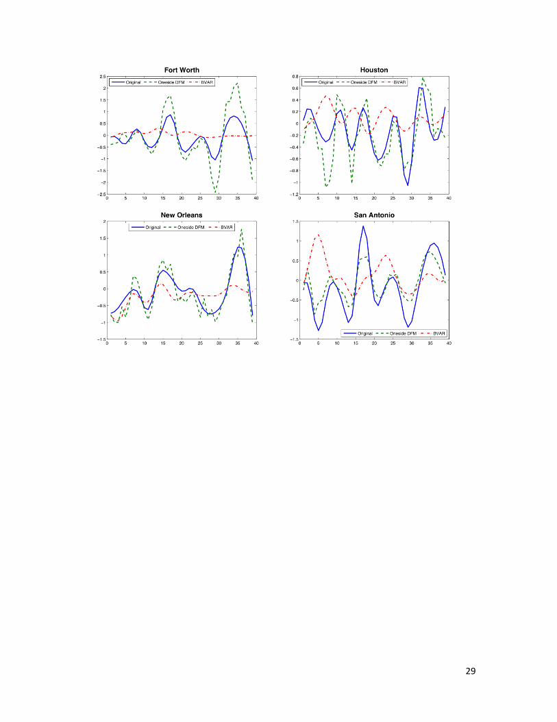
(iv) Comparing the average Theil U-statistics for forecasts of DFM with those of
LBVAR, DFM has a much better forecasting performance than its LBVAR
alternative. Except for the third metro group, the U-statistics of DFM are almost
only half of those for LBVAR model. The U-statistic measures the ratio of the
root mean square error (RMSE) of the model forecasts to the RMSE of naïve, no-
change forecasts. Thus the results imply that the RMSE of DFM is about only half
of the RMSE of LBVAR. The superiority of DFM over its alternative is also easy
to see from Figure 1, which plots the out-of-sample forecasts of both DFM and
LBVAR, and compares them to the actual series for all 42 metropolitan areas.
(v) Comparing across the four Tables, DFM predicts the house price growth rates of
the second metro group the most accurately, and the ones of the third metro group
most poorly. However, LBVAR model performs best in analyzing the third metro
group—the average U-statistic of the optimal LBVAR model for this group is the
lowest among the entire average U-statistics for LBVAR.
(vi) According to Figure 1, DFM can predict the turning points well, but it tends to
overestimate the vibration at the turning point, and also tends to undersmooth the
original data. LBVAR does poorly in turning point prediction.
In summary, DFM consistently outperforms its LBVAR alternative for both the
overall U.S. housing market and the three metro groups. The forecasting power of DFM
does not decrease as the number of forecasted period ahead increases, while LBVAR has
its best performance for two-month-ahead forecast and then its forecasting accuracy

16
decays. The housing price growth rates in the third metro group are affected by the near
lags to a larger extent than the than those in the other two metro groups and the overall
U.S. housing market. DFM can predict turning points well for all metropolitan areas, but
it tends to undersmooth the original data and overestimate the vibration at the turning
points.
5. Conclusion
This paper investigates the recent moving trends of house prices in 42 metropolitan areas
in the United State from the perspective of large-scale models, which are Dynamic Factor
Model (DFM) and Large-scale Bayesian Vector Autoregressive (LBVAR) model. These
models accommodate a large panel data comprising 183 monthly series for the U.S.
economy, and an in-sample period of 1980:01 to 2007:12 are used to forecast one- to six-
months-ahead house price growth rate over the out-of-sample horizon of 2008:01 to
2010:12. The 42 metropolitan areas can be divided into three groups based on their house
price patterns. The forecasting power of these two large-scale models are examined based
on their ability to predict the turning points and patterns of house prices in the three
metropolitan groups during the economic recession, and it is measured in terms of the
Theil U statistic.
Our results show that DFM consistently outperforms its LBVAR alternative for
both the overall U.S. housing market and three metropolitan (metro) groups. The
forecasting power of DFM does not decrease as the number of forecasted period ahead
increases, while LBVAR has its best performance for two-month-ahead forecast and then
its forecasting accuracy decays. The housing price growth rates of the third metro group
are affected by the near lags to a larger extent than the than those in the other two metro
groups and the overall U.S. housing market. DFM can predict turning points well for all
metropolitan areas, but it tends to undersmooth the original data and overestimate the
vibration at the turning points.
The poor forecasting performance of LBVAR model may be due to the two major
limitation of this method. First, the forecast accuracy is sensitive to the choice of the
priors. So if prior is not well specified, an alternative model used for forecasting may

17
perform better. Secondly, the selection of the prior based on some objective function for
the out-of-sample forecasts may not be „optimal‟ for the time period beyond the period
chosen to produce the out-of-sample forecasts (Das, Gupta, and Kabundi, 2008, 2009a)
Although DFM is the better model to base one‟s forecasts on, there are two caveats
in its application. First, structural changes of the economy, whether in or out of the
sample, would make the models inappropriate. Second, the estimation procedures used
are linear in nature, and hence, they fail to take into account of the nonlinearities in the
data (Das, Gupta, and Kabundi, 2009a).

18
Reference
Bloor, C., T. Matheson. “Analyzing Shock Transmission in a Data-Rich Environment: A
Large BVAR for New Zealand.” Empirical Economics 39(2010): 537-558.
Boivin, J., M.P. Giannoni, and I. Mihov. “Sticky Prices and Monetary Policy: Evidence
from Disaggregated US Data.” American Economic Review 99(2009):350-384.
Das, S., R. Gupta, and A. Kabundi. “Is a DFM Well-Suited in Forecasting Regional
House Price Inflation?” Working paper No. 200814, Dept. of Econ., University of
Pretonia, 2008.
Das, S., R. Gupta, and A. Kabundi. “Could We Have Predicted the Recent Downturn in
the South African Housing Market?” Journal of Housing Economics 4(2009a):325-335.
Das, S., R. Gupta, and A. Kabundi. “The Blessing of Dimensionality in Forecasting Real
House Price Growth in the Nine Census Divisions of the US.” Working paper No.
200902, Dept. of Econ., University of Pretonia, 2009b.
Das, S., R. Gupta, and A. Kabundi. “Forecasting Regional House Price Inflation: A
comparison between Dynamic Factor Models and Vector Autoregressive Models.”
Journal of Forecasting 30(2011): 288-302.
Doan, T.A., R.B. Litterman, and C.A. Sims. “Forecasting and Conditional Projection
Using Realistic Prior Distributions.” Econometric Reviews 3(1984): 1-100.
Dua, P., and S.C. Ray. “ A BVAR Model for the Connecticut Economy.” Journal of
Forecasting 14(1995):167-180.
Forni, M., M. Hallin, M. Lippi, and L. Reichlin. “The Generalized Dynamic-Factor
Model: Identification and Estimation.” The Review of Economics and Statistics 4(2000):
540-554.
Forni, M., M. Hallin, M. Lippi, and L. Reichlin. “Do financial vairables help forecasting
inflation and real activity in the euro area?” Journal of Monetary Economics 6(2003):
1243-1255.
Forni, M., M. Hallin, M. Lippi, and L.Reichlin. “The Generalized Dynamic Factor Model,
One Sided Estimation and Forecasting.” Journal of the American Statistical Association
100(2005): 830-840.
Gupta, R., A. Kabundi. “Forecasting Macroeconomic Variables Using Large Datasets:
Dynamic Factor Model versus Large-Scale BVARs” Working paper No. 200816, Dept.
of Econ., University of Pretonia, 2008a.

19
Gupta, R., A. Kabundi. “A Dynamic Factor Model for Forecasting Macroeconomic
Variables in South Africa.” Working Paper No. 200815, Dept. of Econ., University of
Pretonia, 2008b.
Gupta, R., A. Kabundi, and S.M. Miller. “Forecasting the US Real House Price Index:
Structural and Non-Structural Models with and without Fundamentals.” Working paper
No. 200927, Dept. of Econ., University of Pretonia, 2009a.
Gupta, R., A. Kabundi, and S.M. Miller. “Using Large Data Sets to Forecast Housing
Prices: A Case Study of Twenty US States.” Working paper No. 200905, Dept. of Econ.,
University of Pretonia, 2009b.
Gupta, R., S.M. Miller, D.V. Wyk. “Financial Market Liberalization, Monetary Policy,
and Housing Price Dynamics.” Working paper No. 201009, Dept. of Econ., University of
Pretonia, 2010.
Himmelberg, C., C. Mayer, and T. Sinai. “Assessing High House Prices: Bubbles,
Fundamentals and Misspecifications.” Journal of Economic Perspective 19(2005):67-92.
Jolliffe, I.T. (2002). Principal Component Analysis. New York: Springer-Verlag.
Linneman, P. “An Empirical Test of the Efficiency of the Housing Market.” Journal of
Urban Economics 20(1986): 140-154.
Litterman, R.B. “Forecasting with Bayesian Vector Autoregression- Five Years of
Experience.” Journal of Business and Economic Statistics 4(1986):25-38.
Litterman, R.B. “A Bayesian Procedure for Forecasting with Vector Autoregressions.”
Working paper, Federal Reserve Bank of Minneapolis (1981).
Quigley, J.M. “Real Estate Prices and Economic Cycles.” International Real Estate
Reviews 2(1999): 1-20.
Rapach, D.E., and J.K. Strauss. “Difference in Housing Price Forecast Ability across U.S.
States.” International journal of Forecasting 25(2009): 351-372.
Spencer, D.E. “Developing a Bayesian Vector Autoregression Forecasting Model.”
International Journal of Forecasting 9(1993): 407-421.
Stock, J.H., and M.W. Watson. “Macroeconomic Forecasting Using Diffusion Indexes.”
Journal of Business and Economic Statistics 2(2002): 147-162.
Stock, J.H., and M.W. Watson. “Forecasting Output and Inflation: The Role of Asset
Prices.” Journal of Economic Literature 3(2003):788-829.

20
Todd, R.M. “Improving Economic Forecasting with Bayesian Vector Autoregression.”
Quarterly Review (Federal Reserve Bank of Minneapolis) (Fall, 1984): 18-29.
Tsatasaronis, K., and H. Zhu. “What Drives Housing Price Dynamics: Cross-Country
Evidence.” BIS Quarterly Review March, 2004:65-78.
Weathon, W.C. “Real Estate „Cycle‟: Some Fundamentals.” Real Estate Economics 27
(1999): 209-230.

21
Table 1: Metropolitan areas with three price patterns
Group One
Markets where house prices peaked in the late 1980s and had a trough in the 1990s:
Atlanta, GA Nashville, TN Richmond, VA
Austin, TX New York, NY Sacramento, CA
Baltimore, MD Oakland, CA San Diego, CA
Boston, MA Philadelphia, PA San Francisco, CA
Dallas, TX Phoenix, AZ San Jose, CA
Jacksonville, FL Portland, OR Seattle, WA
Los Angeles, CA Raleigh-Durham, NC
Group Two
Markets where house prices were high in the early 1980s and rebounded in the 2000s:
Charlotte, NC Detroit, MI Milwaukee, MN
Chicago, IL Fort Lauderdale, FL Minneapolis, MN
Cincinnati, OH Indianapolis, IN Orlando, FL
Cleveland, OH Kansas City, KS Pittsburgh, PA
Columbus, OH Memphis, TN St. Louis, MO
Denver, CO Miami, FL Tampa, FL
Group Three
Markets where house prices have declined since the early 1980s and never fully
rebounded:
Fort Worth, TX New Orleans, LA San Antonio, TX
Houston, TX

22
Table 2: One- to Six-Months-Ahead Theil U-statistics for All the Metropolitan Areas
Model 1 2 3 4 5 6 Average
DFM 0.3440 0.3440 0.3440 0.3440 0.3440 0.3440 0.3440
w=0.1, d=0.5 LBVAR 0.7037 0.6802 0.7235 0.7877 0.8120 0.8163 0.7539
w=0.1, d=1.0 LBVAR 0.7113 0.6889 0.7322 0.7945 0.8171 0.8207 0.7608
w=0.1, d=2.0 LBVAR 0.7065 0.6833 0.7233 0.7835 0.8047 0.8072 0.7514
w=0.2, d=0.5 LBVAR 0.6911 0.6653 0.7071 0.7737 0.8034 0.8147 0.7426*
w=0.2, d=1.0 LBVAR 0.6978 0.6735 0.7176 0.7818 0.8090 0.8177 0.7496
w=0.2, d=2.0 LBVAR 0.7127 0.6924 0.7377 0.7970 0.8187 0.8239 0.7637
w=0.3, d=0.5 LBVAR 0.6956 0.6692 0.7089 0.7739 0.8059 0.8249 0.7464
w=0.3, d=1.0 LBVAR 0.6933 0.6669 0.7093 0.7745 0.8054 0.8205 0.7450
w=0.3, d=2.0 LBVAR 0.7104 0.6886 0.7358 0.7967 0.8218 0.8312 0.7641
Table 3: One- to Six-Months-Ahead Theil U-statistics for Metro Group One
Model 1 2 3 4 5 6 Average
DFM 0.3150 0.3150 0.3150 0.3150 0.3150 0.3150 0.3150
w=0.1, d=0.5 LBVAR 0.7004 0.6872 0.7302 0.8008 0.8364 0.8325 0.7646
w=0.1, d=1.0 LBVAR 0.7082 0.6956 0.7385 0.8066 0.8402 0.8357 0.7708
w=0.1, d=2.0 LBVAR 0.7034 0.6896 0.7294 0.7946 0.8246 0.8178 0.7599
w=0.2, d=0.5 LBVAR 0.6872 0.6727 0.7143 0.7916 0.8371 0.8429 0.7576*
w=0.2, d=1.0 LBVAR 0.6936 0.6805 0.7251 0.7977 0.8388 0.8408 0.7628
w=0.2, d=2.0 LBVAR 0.7105 0.7014 0.7474 0.8130 0.8465 0.8437 0.7771
w=0.3, d=0.5 LBVAR 0.6967 0.6830 0.7218 0.7989 0.8480 0.8631 0.7686
w=0.3, d=1.0 LBVAR 0.6900 0.6750 0.7175 0.7938 0.8415 0.8523 0.7617
w=0.3, d=2.0 LBVAR 0.7078 0.6976 0.7461 0.8153 0.8552 0.8580 0.7800

23
Table 4: One- to Six-Months-Ahead Theil U-statistics for Metro Group Two
Model 1 2 3 4 5 6 Average
DFM 0.3419 0.3419 0.3419 0.3419 0.3419 0.3419 0.3419
w=0.1, d=0.5 LBVAR 0.6965 0.6670 0.7162 0.7852 0.8050 0.8159 0.7476
w=0.1, d=1.0 LBVAR 0.7040 0.6762 0.7258 0.7933 0.8117 0.8220 0.7555
w=0.1, d=2.0 LBVAR 0.6989 0.6708 0.7171 0.7841 0.8029 0.8125 0.7477
w=0.2, d=0.5 LBVAR 0.6832 0.6512 0.6991 0.7667 0.7885 0.8045 0.7322*
w=0.2, d=1.0 LBVAR 0.6913 0.6606 0.7101 0.7769 0.7972 0.8112 0.7412
w=0.2, d=2.0 LBVAR 0.7049 0.6784 0.7290 0.7929 0.8094 0.8211 0.7559
w=0.3, d=0.5 LBVAR 0.6815 0.6487 0.6955 0.7604 0.7837 0.8067 0.7294
w=0.3, d=1.0 LBVAR 0.6848 0.6526 0.7011 0.7665 0.7882 0.8070 0.7334
w=0.3, d=2.0 LBVAR 0.7041 0.6759 0.7276 0.7905 0.8075 0.8221 0.7546
Table 5: One- to Six-Months-Ahead Theil U-statistics for Metro Group Three
Model 1 2 3 4 5 6 Average
DFM 0.6354 0.6354 0.6354 0.6354 0.6354 0.6354 0.6354
w=0.1, d=0.5 LBVAR 0.8461 0.7777 0.7393 0.7075 0.6923 0.6943 0.7429
w=0.1, d=1.0 LBVAR 0.854 0.7852 0.7447 0.7097 0.6928 0.6947 0.7468
w=0.1, d=2.0 LBVAR 0.8516 0.7799 0.7322 0.6913 0.6731 0.6801 0.7347
w=0.2, d=0.5 LBVAR 0.8518 0.7713 0.727 0.6948 0.6794 0.6828 0.7345
w=0.2, d=1.0 LBVAR 0.8431 0.7668 0.7282 0.7004 0.6888 0.6934 0.7368
w=0.2, d=2.0 LBVAR 0.8515 0.7796 0.7411 0.7074 0.692 0.695 0.7444
w=0.3, d=0.5 LBVAR 0.8764 0.7836 0.7329 0.6967 0.6785 0.6802 0.7414
w=0.3, d=1.0 LBVAR 0.8536 0.7668 0.7219 0.6941 0.6822 0.6874 0.7343*
w=0.3, d=2.0 LBVAR 0.8347 0.7593 0.7272 0.7044 0.6961 0.7011 0.7371

24
Figure 1: Original data and forecasts from DFM and LBVAR model for the 42
metropolitan areas from 2008:M1-2010M12

25

26

27

28
29