forecasting bitcoin prices
TRANSCRIPT

1
FORECASTING BITCOIN PRICES
ARIMA vs LSTM
João Filipe Batista Mendes
Dissertation submitted as partial requirement for the conferral of
Master in Economics
Supervisor:
Prof. Vivaldo Mendes
Co- Supervisor:
Prof. Diana Mendes
September 2019

2
Abstract
Bitcoin has recently received special attention in economics and finance as the
most popular blockchain technology. This dissertation aims to discuss whether
newly machine-leaning models perform better than traditional models in
forecasting. Particularly, this study compares the accuracy of the prediction of
bitcoin prices using two different models: Long-Short Term Memory (LSTM)
versus Auto Regressive Integrated Moving Average (ARIMA), in terms of
forecasting errors, and Python routines were used for such purpose. Bitcoin price
time series ranges from 2017-06-18 to 2019-08-07, in a daily basis, sourced from
the Federal Reserve Economic Data. To compare the results of both models, data
was divided into two subsets: training (83.5%) and testing (16.5%). The literature
usually indicates that LSTM outperforms ARIMA. In this dissertation, the results
do confirm that LSTM forecasts of bitcoin prices improve on average ARIMA
predictions by 92% and 94%, according to RMSE and MAE.
Keywords: ARIMA, LSTM, Bitcoin, Forecasting.

3
Resumo
A Bitcoin tem recebido recentemente especial atenção em áreas como a economia
e finanças por ser a mais popular tecnologia de blockchain. Esta dissertação tem
como objetivo verificar se os novos modelos de machine-learning apresentam
melhores resultados que os modelos tradicionais em previsões. Este estudo
compara, em particular, a precisão da previsão do preço da Bitcoin usando dois
modelos diferentes: Long-Short Term Memory (LSTM) versus Auto Regressive
Integrated Moving Average (ARIMA), em termos de erros de previsão e aplicando
rotinas do Python. A análise teve como base os preços diários da Bitcoin entre 18
de junho de 2016 e 7 de agosto de 2019, retirados da base de dados da Reserva
Federal. Para comparar os resultados dos dois modelos, os dados foram divididos
em duas secções: o treino (83.5%) e o teste (16.5%). A literatura indica que o
modelo LSTM tem uma melhor precisão que o ARIMA e nesta dissertação os
resultados confirmam que o modelo LSTM melhora em média 92% e 94% a
previsão do ARIMA, de acordo com o RMSE e o MAE.
Palavras chave: ARIMA, LSTM, Bitcoin, Previsão

4
Acknowledgements
Thanks to all professors who make part of this long journey.
Thanks to my supervisors for their support, patience and motivation to help me.
Thanks to Prof. Diana Mendes for her special support in computing python codes.
Thanks to my friends who always encourage me.
Thanks to my girlfriend who always supports me and motivates me.
Thanks to my parents who always believe in me and never let me give up.

5
List of Figures
Figure 3.1 - Time series divided into training data and test data……………… 20
Figure 3.2 - Multi-layer perceptron…………………………………………... 24
Figure 3.3 – Activation function……………………………………………... 24
Figure 3.4 - Recurrent neural network with p time steps…………………...... 26
Figure 3.5 - LSTM cell and its operations ………………………………....... 28
Figure 4.1 - Bitcoin Price time series ………………………………………... 29
Figure 4.2 - Bitcoin Price time series divided between training and testing…. 30
Figure 5.1 - ACF and PACF function…………………………………………32
Figure 5.2 - First differences…………………………………………………. 32
Figure 5.3 - ARIMA (1,1,1) model results…………………………………… 33
Figure 5.4 - ARIMA (1,1,1) forecasting. Forecasts and bitcoin observations… 34
Figure 5.5 - Residuals plot for ARIMA predictions…………………………... 34
Figure 5.6 - ARIMA (1,1,1) forecasting. Training data, testing data and
forecasts……………………………………………………………………. 35
Figure 5.7 - LSTM layers shape……………………………………………… 37
Figure 5.8 - Value Loss and Loss Functions…………………………………. 37
Figure 5.9 - LSTM forecasting. Observed values and prediction values……… 38
List of Tables
Table 5.1- ADF test results…………………………………………………... 31
Table 5.2- ADF critical values……………………………………………… 31
Table 5.3- AIC score of different order ARIMA model………………………33
Table 5.4 - RMSE and MAE forecasting errors for both ARIMA and LSTM
models……………………………………………………………………… 39
List of Equations
Equation 3.1 - Auto-regressive (AR) model…………………………………. 21
Equation 3.2 - Moving averages (MA) model………………………………… 22
Equation 3.3 - ARMA (p, q) model……………………………………………22
Equation 3.4, 3.5 and 3.6 - input (ot), forget (gt) and output (ct) gates……... 27
Equations 3.7, 3.8 and 3.9 - internal hidden state……………………………. 27
Equation 5.1 - MAE…………………………………………………………... 39
Equation 5.2 - RMSE………………………………………………………… 39
6
List of abbreviations
ACF - Autocorrelation function
ADF – Augmented Dickey Fuller
AIC – Akaike Information Criterion
ANN - Artificial Neural Networks
AR – Auto Regressive
ARMA – Auto Regressive Moving Average
ARIMA - Auto Regressive Integrated Moving Average
GARCH - Generalized Autoregressive Conditional Heteroskedasticity
LSTM - Long-Short Term Memory
MA - Moving-average
MAE - Moving Average Error~
P2P - Peer-to-peer
PACF - Partial autocorrelation
RNN - Recurrent Neural Network
RMSE - Root Mean Squared Error
VEC - Vector Error Correction
7
Contents
1. Introduction ...................................................................................................... 8
2. Literature Review ........................................................................................... 10
2.1 Bitcoin .......................................................................................................... 10
2.1.1. Pre-Bitcoin ............................................................................................... 10
2.1.2. Bitcoin and Blockchain ............................................................................ 11
2.1.3. Pros and cons of Bitcoin .......................................................................... 12
2.1.4. Alternative cryptocurrencies .................................................................... 15
2.2. Previous research ........................................................................................ 16
3. Forecasting Models Background.................................................................... 20
3.1. Time Series Forecasting .............................................................................. 20
3.2. Forecasting models...................................................................................... 21
3.2.1 ARIMA ..................................................................................................... 21
3.2.2 Non-linear machine learning models ........................................................ 23
3.2.2.1. ANN ...................................................................................................... 23
3.2.2.2. RNN ...................................................................................................... 25
3.2.2.3. LSTM .................................................................................................... 26
4. Data ................................................................................................................ 29
5. Models Implementation ................................................................................. 31
5.1. ARIMA ....................................................................................................... 31
5.2. LSTM .......................................................................................................... 36
5.3 Results .......................................................................................................... 39
6. Conclusion ..................................................................................................... 40
7. References ...................................................................................................... 42
8. Annexes .......................................................................................................... 45
8.1 – ARIMA algorithm ..................................................................................... 45
8.2 – LSTM algorithm ....................................................................................... 50

8
1. Introduction
Forecasting economical and financial time series data is a challenging mission
due to uncertain events or incomplete information in the economies we live in.
This situation produces high levels of volatility in time series. In order to predict
more accurately, authors have applied over time more and more sophisticated
forecasting techniques.
The aim of this dissertation is to investigate whether the machine learning models
offer or not better predictions than traditional models in terms of lower
forecasting errors and higher accuracy in forecasts. More specifically, I will
compare the Auto Regressive Integrated Moving Average (ARIMA) and Long-
Short Term Memory (LSTM), a specific type of Recurrent Neural Network
(RNN).
In this dissertation, I will use Spyder (Python 3.6) to run Python codes1 in order
to estimate both models. Why Python? Python is a freeware /open source
dynamic language and very appropriate to interactive development. It is also
widely used in machine learning and data science due to its library support. In
order to run programs in Python it is necessary to import some important libraries
for time series such as: NumPy providing efficient array operations; Matplotlib
for plotting data; Pandas providing high performance tools for loading and
handling data; Statsmodels providing statistical modelling and Scikit learn
helping to develop and practice machine learning in Python.
In recent years, bitcoin has been established as the world leading cryptocurrency
taking the attention of consumers, businesses and investors. As a result of bitcoin
network complexity, I would like to investigate some of the techniques of
machine learning in order to forecast bitcoin prices.
This remaining part of this dissertation is organized in six chapters. Chapter 2
deals with a literature review and is divided in two parts. In the first one, I
describe the functioning of the bitcoin and a blockchain, give a brief description
1 See Annexes in Chapter 8

9
about what happened before the appearance of this cryptocurrency, present also
some pros and cons of such currency, and describe some alternative
cryptocurrencies that have recently challenged the bitcoin. In the second part, I
present some previous research about the bitcoin including studies comparing
traditional econometric models with newly machine-learning approaches. In
Chapter 3, I provide some insights related to both models: ARIMA and LSTM,
in terms of forecasting. To understand better the LSTM approach, I also introduce
in this section the Artificial Neural Networks (ANN) and Recurrent Neural
Network (RNN). In Chapter 4, I describe the data used across this dissertation.
In Chapter 5, I implement each model, step by step, in order to get the forecast
of bitcoin prices according to our methodology. Also, I compare the results of
both models in terms of forecasting errors, specifically Root Mean Squared Error
(RMSE) and Moving Average Error (MAE). In Chapter 6, I summarize the
results, stress the main findings of this dissertation, and will suggest also some
points that may deserve further research.
10
2. Literature Review
2.1 Bitcoin
2.1.1. Pre-Bitcoin
According to Nathan Reiff’s article (Reiff, 2019), one of the first attempts to
create a cryptocurrency comes from Netherlands in late 1980s. Petrol stations
were suffering from thefts and a group of people tried to link money to new
smartcards instead of using cash.
At the same time, an American cryptographer David Chaum introduced a
different electronic cash, digiCash (Chaum, 1983). He developed a “blinding
formula” to encrypt information to be passed among people. This tool could
allow money to be sent safely between individuals only by checking the signature
authenticity. This innovation played an important role in future cryptocurrencies.
Some companies applied these fundamentals in the 1990s. The company with the
greatest lasting impact was PayPal. This world known enterprise modernized
person-to-person online payments. Individuals could quickly and securely
transfer money via internet. One of the most successful applications was the e-
gold, which offered to users the chance to use money in exchange of physical
gold or other metals.
In 1998, Wei Dai developed an “anonymous, distributed electronic cash system”,
called b-Money (Dai, 1998). This system was based on a digital pseudonym used
to transfer currency through a decentralized network. The structure also included
a contract in network as well rather than a third party. Even though it was not as
successful as other cryptocurrencies were, Nakamoto (2008) referenced some
points of B-money in his bitcoin whitepaper.
Developed in mid-1990s, Hashcash (Back, 1997) was one of the most effective
pre-bitcoin digital currencies. It used proof-of-work algorithms to create and
distribute new coins.

11
The Bit Gold proposed by Szabo (2008) introduced a proof-of-work system,
which is used in some ways in bitcoin’s mining network. In the next sub-section,
I will explore the functioning of the main cryptocurrency – the bitcoin.
2.1.2. Bitcoin and Blockchain
A Blockchain is a distributed database of records that have been performed and
shared among the involved parties. The majority of participants in the network
revises each transaction. As soon as the information entered in the system, it can
never be removed. The Bitcoin is the most popular example of the blockchain
technology.
“Bitcoin is a peer-to-peer electronic cash system” introduced in the well-known
paper Nakamoto (2008). The peer-to-peer (P2P) mechanism allows an ownership
transfer from one party to another without a third-party intervention (financial
institution). Payments can be made over the internet without any control or cost
of a central authority for the first time. Individuals who want to own bitcoins can
either run a program on their own computer that implements bitcoin protocol, or
create an account on a website that runs bitcoin for its users. The bitcoins are
saved in a file called wallet, which the user may secure and backup. These
programs connect to each other over the internet forming P2P networks, making
the system resistant to a central attack (Zohar, 2015) and (Crosby et al., 2016).
For now, Bitcoins are generated through a process of mining. Any member
operates as a miner using their computer knowledge to maintain the network.
Mining is a computationally process that requires miners to find a solution to a
mathematical problem in order to create a new block into the blockchain. Miners
resolve this issue by using the proof-of-work concept. This algorithm involves
recurrently difficult mathematical problems until getting to a solution. The first
miner to find a solution broadcasts it to the network to verify it. Once verified the
block is added to the blockchain. Every ten minutes on average is found a new
answer and a bitcoin is created. The bitcoin protocol is designed to generate a

12
new bitcoin gradually. The difficulty of solving problems is adjusted every two
weeks at the rate of six blocks per hour. The size of the reward was initially 50
(genesis block) and it is halved every four years, this implies that the number of
bitcoins in circulation will never exceed 21 million. Once the last bitcoin is
generated, miners will instead be rewarded with transactions fees (Zohar, 2015)
and (Crosby et al., 2016).
The core principle of bitcoin technology is public-key cryptographic. This
method determines that each transaction is protected through a digital signature
and verified by every node in the network. It uses an algorithm that generates two
separate keys: the public key and private key. In this system, the sender sends his
private key digitally signed to the public key of the receiver. In order to complete
the transaction, the sender needs to prove his ownership and the receiver needs
to verify that ownership by using the information received in the public key. The
verifying nodes have to ensure that the spender owns the cryptocurrency through
the digital signature and to confirm that the spender has enough cryptocurrencies
in his account to complete the transaction by checking his account or validating
in the public key. New transactions are checked against the blockchain to make
sure that the bitcoins were already spent, thus solving the double spending
problem. Each transaction has a digital signature and a hash containing all the
chronological history of movements and peers that allows for easy detection in
case of double-spending attacks. (Zohar, 2015) and (Crosby et al., 2016).
According to Velde (2013), “bitcoin solves two challenges of digital money-
controlling its creation and avoiding its duplication- at once.” Nakamoto (2008)
showed that as long as attackers do not have more than 50% of the computer
power of the network, the probability of a successful attack is almost null.
In the next sub-section, I will discuss some of pros and cons of bitcoin.
2.1.3. Pros and cons of Bitcoin
Bitcoin as a new technology brings a wide range of benefits and risks to the table.

13
This cryptocurrency was specifically designed for fast transactions at low costs
as said by Nakamoto (2008). A low-cost transaction is possible because there is
no-single party intermediary. “Users have full control of their bitcoins and the
freedom to send and receive bitcoins anytime, anywhere and from anyone.” as
said by Nian & Lee (2015). Each bitcoin can only be processed by the user who
has access to the private key, giving to him full control of his bitcoins. Bitcoin
can also be considered as an alternative to other electronic methods of payment
accepted by businesses. In its original form, the bitcoin protocol works
essentially as a payment network, but it has potential for further innovation, as
developed from other cryptocurrencies.
In the previous years, Bitcoin has become a fixture in world financial news.
However, should bitcoin be a considered a currency? Money is typically defined
by economists as having three attributes: medium of exchange, a unit of account,
and a store of value. “Bitcoin does not behave much like a currency according to
the criteria widely used by economists. Instead, Bitcoin resembles a speculative
investment similar to the Internet shocks of the late 1990s” (Yermack, 2015). In
his point of view, Bitcoin has no intrinsic value since it is useless as a currency
in the consumer theory. As said by Krugman (2018) “The modern dollar (…) is
ultimately backed by the fact that the U.S government will accept it. Its
purchasing power is also stabilized by the Federal Reserve.” “Bitcoin, by
contrast, has no intrinsic value. (…) You have an asset whose price is almost
purely speculative, and hence incredibility volatile.”
According to data available in bitcoin websites, most of bitcoin transactions
involve transfers between speculative investors and only a minority are used for
purchases of goods and services. Bitcoins require the merchant and the consumer
to wait on average 10 minutes of verification to finalize a transaction. According
to Velde (2013), “A dollar bill in my hand cannot be anywhere else at the same
time, my ownership of it is undoubted, and it can be exchanged immediately.”
By contrast, “bitcoin try to emulate these properties of cash, but do so at some
costs.” Yermack (2015) notes that a currency to role as a unit of account,
14
customers should be able to compare the price of goods. Bitcoin faces extreme
volatility compared to other currencies on a daily-to-daily basis. Prices would
change frequently in terms of bitcoins and, therefore, this uncertainty of market
value would create distrust in transactions with bitcoins. When currency works
as a store of value, the owner expects to receive the same economic value that
the currency was worth when acquired it. Holding bitcoins even for a shorter
period is quite risky due to the high volatility, which is inconsistent with the idea
of stability of a currency as a store of value. Athey et al. (2016) reveal in their
paper that users are not active and that many buy and hold bitcoins. Due to bitcoin
potential users tend to save bitcoins than spend it, creating a moral hazard issue.
The anonymity and ease of payments offered by Bitcoin may also facilitate
criminal activities. Yermack (2015) gives the example of Silk Road internet
portal used for selling illegal narcotics that only accepted bitcoins as payment.
Nian & Lee (2015) present another major concern regarding Bitcoin which is
money laundering and finance terrorist activity. Krugman (2018) reinforces the
idea that bitcoin price might be influenced by some fraudulent activities, “Back
in 2013 fraudulent activities by a single trader appear to have caused a sevenfold
increase in Bitcoin’s price.” Stiglitz in a CNBC video on May 2019 said that “I
actually think we should down the cryptocurrencies.” According to him, crypto
is not the right way to create a more efficient global economy due to the lack of
transparency related to illegal financial activities such as money laundering.
However, bitcoin also offers protection against some forms of financial crimes
since the mining process of verifying transactions solves the double-spending
issue. It is hard to overcome the combined computer network.
The regulatory landscapes continue to change across countries as governments
struggle with the risks and benefits of bitcoin, for example in the incentives of
tax evasion due to uncertain tax treatment in bitcoin network. For example,
Schilling & Uhlig (2019) concludes that “Bitcoin block rewards are not a tax on
bitcoin holders: they are financed with a Dollar tax.” For example, bitcoin is legal
in USA and EU, but in China, only private persons can hold bitcoin. In December

15
2013, the People’s Bank of China, the central bank of China, banned Chinese
banks from relationships with bitcoin exchanges (Bӧheme et al., 2015).
Bitcoin is very different from the existing financial system for which regulators
are used to deal with. Bitcoin can easily scale up and destabilize the economy
and the financial markets. Krugman (2018) considers clearly that bitcoin is a
bubble where early investors make a lot of money as new investors draw in,
pulling even more people in the network. For him, this process will have a painful
end.
Finally, there is some intrinsic risks directly related to technology dependence of
bitcoin. Athey et al., (2016) states “the risk of failure of a technology” like an
operator error in the system, security flaws or even a malware that affects the
hard drives and consequently the private keys.
After the creation of bitcoin several other cryptocurrencies were introduced to
mitigate some of the risks previously mentioned. In the next sub-section, I will
describe briefly some alternative cryptocurrencies.
2.1.4. Alternative cryptocurrencies
Most of alt-coins are derived from bitcoin’s source code (“forks”). Some are
implemented based on the blockchain model without using any of bitcoin’s code.
Mostly, there are two separate applications of blockchain technology, one used
predominantly as currency (alt-coin), whereas alt-chain are used for other
purposes, not necessary currency (Antonopoulos, 2014).
The first alt-chain appeared in August 2011, called Namecoin. In the same month,
the first alt-coin IXCoin was launched with some new specifications as the major
reward of 96 coins per block. In the following month, Tenebrix introduce an
alternative concept of proof-to-work, namely script, an intense algorithm
designed for password stretching. This last currency was one of the basis for the
creation of Litecoin, which also applied a script proof-to-work algorithm. This

16
new cryptocurrency has a faster block generation time, target to 2.5 minutes
instead of 10 minutes of bitcoin. In one-year time, several alt coins were created.
In the beginning of 2013, there were about 20 alt coins and by the end of the same
year, the number boomed to 200. In 2014, the growth of at coins continued, being
500 most of them replicas of Litecoin (Antonopoulos, 2014).
Alt-chains are alternative implementations of the blockchain, which are not
necessary currency. Alt-chains are used an alternative platform such as a
contract. Ethereum is an example of turing-complete contract processing and
execution platform based on blockchain. An independent design with an own
currency called ether, necessary to use for contract execution. Mostly, a contract
is a program that runs in every node in the ethereum network. These contracts
can collect date, send and receive payments, execute an infinite sort of
computable actions and store ether (Antonopoulos, 2014).
The future of cryptocurrencies is overall so bright. Bitcoin introduced a new form
of de-centralized system. It has reproduced hundreds of incredible innovations,
which has affected sectors such as economics, finance, science, baking and
corporate governance.
2.2. Previous research
Since Bitcoin appears in 2008 (Nakamoto, 2008), many academic papers have
focused on it from different perspectives. Some authors examined the bitcoin’s
potential and its impact in other economic variables using traditional econometric
approaches. The GARCH (Generalized Autoregressive Conditional
Heteroskedasticity) framework showed several similarities between gold and US
dollar in terms of hedging abilities and advantages in exchange. For Dyhrberg
(2015), bitcoin has a position in financial markets and project management
between gold and American dollar with clear advantages to risk adverse
investors. Alternatively, some authors performed a cointegration analysis to
examine the impact of some variables on bitcoin price. For ecample, Ciaian et

17
al., (2015) found a significant impact of global macro-financial development
captured by the Down Jones index, exchange rate and oil price, only in the short-
run, by using the gold standard model by Barro (1979). In long-run, these
variables do not determine the bitcoin price. Alternatively, Zhu et al. (2017)
suggested that some factors such as Consumer Price Index, Down Jones industry
average and Fed Funds Rate do have long run negative effect on bitcoin price, by
applying VEC (Vector Error Correction) model. However, gold price is barely a
factor to influence bitcoin price. Thus, bitcoin may not hedge against the gold
price. “Bitcoin is more an asset rather than a currency.” Zhu et al. (2017).
Due to the importance of forecasting in many branches of science, many
specialists have developed a variety of the time series forecasting models. Time
series forecasting is traditionally performed in econometrics using ARIMA
models, which was generalized by Box and Jenkins (1970). Recently, specialists
have been developed new techniques to address new challenges in forecasting by
applying machine-learning models. Long Short-Term Memory is a special case
of Recurrent Neural Network (RNN) that was introduced by Hochreiter &
Schmidhuber (1997). Some years later, Schmidhuber et al., (1999) identified a
weakness of LSTM models that do not clearly identify the end of a network In
order to solve this shortcoming, the authors proposed the “forget gate” that
enables the LSTM model to reset at any time.
Even though it is a quite recent new approach, deep learning models have gained
popularity in forecasting. The papers by Namin and Namin (2018) and
Elmasdotter and Nystromer (2018) compared the effectiveness in forecasting
time series of these two models. In the first paper, the authors predicted stock
market indexes while in the second one, the authors forecasted the grocery store
sales for two different scenarios: one day ahead and seven days ahead, for both
models. In both cases, the authors split data into two subsets: training data and
testing data (70/30) and (80/20), respectively. Therefore, the parameters of
LSTM such as sequence length, dropout rate, epochs and neurons output layer
were adapted according to each scenario. Still, the autoregressive order (p), the

18
order of differencing (d) and the moving average order (q) were adjusted for each
model. In the first paper, the authors compiled the model with the mean squared
error and Adam 2as the loss function and the optimization algorithm. In terms of
error terms, in both papers, the LSTM over performs ARIMA in forecasting. In
the first paper, the LSTM algorithm improved on average 85% the prediction
compared to ARIMA in reduction of error terms for both financial and economic
data. In the second paper, the LSTM model has a lower error overall for one-day
and seven-days ahead scenarios, in terms of RMSE (Root Mean Square Error)
and MAE (Mean Absolute Error).
Research on predicting the bitcoin price has not been much developed. However,
some authors have also compared machine-learning techniques with the
traditional models in forecasting bitcoin prices. McNally (2016) concluded that
traditional ARIMA model forecasting was worse than the neural non-linear
network models (RNN and LSTM) in both criteria, accuracy rate and RMSE. In
addition, the LSTM outperformed the RNN marginally but there was not
significant difference between both, as the LSTM reaches the highest accuracy
rate (53%) and the RMSE of 7%, slightly higher than the RNN. However, the
LSTM takes 3.1 times longer to train applying the same network parameters due
to the high number of activation functions and equations to be performed. Still,
some authors investigated the power of some features on bitcoin price by using
machine-learning optimization. Huisu et al. (2018) established a Rolling Window
LSTM model to predict bitcoin price by selecting some input features relevant to
macroeconomics, global currency ratios and blockchain information. The LSTM
model with rolling window settings overperforms for example the simple LSTM
and Neural Network models by using MAPE and RMSE.
Other authors have developed some sentimental analysis by using machine-
learning optimization to measure the impact of some indicators such as the
bitcoin related tweets or web search media results in bitcoin prices. Stenqvist and
2 “Adam is an algorithm for first-order gradient-based optimization of stochastic objective
functions, based on adaptive estimates of lower-order moments.” (Kingman and Ba, 2015).

19
Lonno (2017) analyzed 2.27 million bitcoin related tweets that could indicate a
bitcoin price change in the near future. The predicted model, based on the
intensity of sentiment fluctuations from one period to the next, showed that
aggregating tweets sentiments over a 30 min period with four shifts forward, and
a sentiment-limited change of 2.2%, yield an 83% accuracy prediction. The
author suggested adapting machine learning to explore further the correlation
between Bitcoin and tweet data. Matta et al. (2015) investigated the relationship
between the bitcoin price and the volume of tweets and or web search media
results. The authors found out a significant cross correlation between bitcoin
price and Google Tends data by applying a sentimental analysis. The authors
proved the importance of considering these particularities as predictors.

20
3. Forecasting Models Background
3.1. Time Series Forecasting
A time-series is a sequence of observations measured sequentially through time.
The observations at different moments in the series correlate with each other in
different ways. Since the successive observations are dependent, future values
may be predicted from the past ones. “Forecasting is about predicting the future
as accurately as possible, given all of the information available, including
historical data and knowledge of any future events that might impact the
forecasts”, as defined by Hyndman and Athanasopoulos (2018), p.9.
There are several models used for time series forecasting that can be classified
between linear and non-linear, univariate and multi-variate. Linear models are
restricted by their assumption of linear behavior in parameters and/or variables,
whereas non-linear models may fit more complex dynamics and functions
accurately. However, linear models such as the ARIMA are well known for their
accuracy and flexibility in the prediction of linear time series, and also for some
occasionally well succeed short-term value or trend predictions in non-linear
processes.
When choosing forecasting models, it is important to separate the available data
into two parts: training and test data, where training is used to estimate the
parameters of a forecasting method and test is used to evaluate its accuracy
(figure 3.1).
Figure 3.1 – Time series divided into training data and test data.3
The accuracy of forecasts can only be determined by considering how well a
model performs on new data that were not used when fitting the model. It is
3 Source: (Hyndman & Athanasopoulos, 2018), Chapter 3.

21
possible to measure the forecasting accuracy by estimating the forecasting errors,
which is the difference between the observed value and its forecast, calculated in
the testing set. When comparing data from the same scale, as it happens with
bitcoin prices, scale-dependent errors are commonly used such as Mean Absolute
Error (MAE) and Root Mean Squared Error (RMSE).
In the following section, I will discuss these two different approaches relevant to
forecast bitcoin price: i) traditional linear econometric models such as ARIMA
and ii) non-linear machine learning models such as LSTM.
3.2. Forecasting models
3.2.1 ARIMA
The Autoregressive Integrated Moving Average (ARIMA) is a linear model,
which combines an AR process, a MA process and an integrated component,
which involves differencing the time series to convert it into a stationary process.
As seen in equation (3.1)4, the auto-regressive (AR) model expresses the time
series 𝑥𝑡 at time 𝑡 as a linear regression of the previous 𝑝 observations, that is:
𝑥𝑡 = 𝛼 + ∑ 𝜙𝑖
𝑝
𝑖=1
𝑥𝑡−𝑖 + 𝜀𝑡 (3.1)
and where 𝜀𝑡 is the white noise residual term and 𝜙𝑖 are real parameters.
In equation (3.2)4, the Moving averages (MA) use dependency between residual
errors to forecast values in the next period. The model helps to adjust to
unpredictable events. The 𝑞𝑡ℎorder moving average model denoted by MA (𝑞)
is defined as follows:
𝑥𝑡 = 𝛼 − 𝜃1𝜀𝑡−1 − 𝜃2𝜀𝑡−2 − ⋯ − 𝜃𝑞𝜀𝑡−𝑞 + 𝜀𝑡 (3.2)
4 Source: (Pal & Prakash ,2017), Chapter 4.

22
where 𝛼 and 𝜃𝑖 are real parameters.
The ARMA model combines the power of AR and MA components together. This
way, an ARMA (𝑝, 𝑞) model incorporates the 𝑝𝑡ℎ order AR and 𝑞𝑡ℎ order MA
model, respectively.
We denote by Φ and θ the AR and MA coefficients vectors. The α and 𝜀𝑡 captures
the intercept and the error term at time 𝑡. The complete ARMA(𝑝, 𝑞) model can
be seen in detail in equation (3.3)4, that is:
𝑥𝑡 = 𝛼 + 𝜙1𝑥𝑡−1 + 𝜙2𝑥𝑡−2 + ⋯ + 𝜙𝑝𝑥𝑡−𝑝 − 𝜃1𝜀𝑡−1 − 𝜃2𝜀𝑡−2 − ⋯
− 𝜃𝑞𝜀𝑡−𝑞 + 𝜀𝑡 (3.3)
ARIMA is a generalization of the ARMA model by including integrated
components, which are useful when data is non-stationary5. The ARIMA applies
differencing on time series to remove non-stationary. The ARIMA (𝑝, 𝑑, 𝑞)
represent the order for AR, MA, and differencing components.
The autocorrelation function (ACF) measures how a series is correlated with
itself at different lags. It can help guide of moving average number of lags (q).
The partial autocorrelation (PACF) function can be interpreted as a regression of
the time series against its past lags. At the same way, it can come up with a
possible order of auto regressive term (p). It is also possible to evaluate the best
ARIMA model by using the Akaike Information Criterion (AIC). After checking
the residuals, it is possible to advance to forecasts calculations.
The model is well known for its forecasting accuracy. However, as it is a linear
model, ARIMA suffers from some limitations handling with non-linear
problems, as it is expected to perform better in shorter time periods of forecasting.
5 “Non-Stationary mostly arises due to the presence of trend and seasonality that affects the
mean, variance, and autocorrelation at different points in time.”, (Pal & Prakash, 2017),
Chapter 2.

23
3.2.2 Non-linear machine learning models
To understand what the Long Short-Term Memory (LSTM) algorithm is and how
it works, I will define and describe briefly the functioning of neural networks
through Artificial Neural Networks (ANN) and Recurrent Neural Network
(RNN).
3.2.2.1. ANN
ANNs are inspired by the neural connections, trying to predict the neural
pathways and their behavior. As much robust and self-adapting the ANNs is,
better solutions will be provided in forecasting non-linear problems. A neural
network consists of simple processing units, the neurons, which are linked via
connections. The strength of a connection between two neurons is called weight.
Those weights can be implemented in a weight matrix or in a weight vector. The
neurons can be grouped in the following layers: input layer, hidden layer and
output layer. In figure 3.2, it can be observed an example of multiple layer neural
network.
Figure 3.2 – Multi-layer perceptron6.
The network input is the result of the propagation function since it receives the
outputs from other nodes and transforms them, based on connecting weights, into
6 Source: (Pal & Prakash ,2017), Chapter 5.

24
the neural input that can be then processed by the activation function. It
transforms the network input as well as the previous state into a new activation
state with a threshold value playing an important role since it marks the position
of the maximum gradient value of the activation function. The most commonly
activation functions used are the sigmoid (sig), hyperbolic tangent (tan) and a
Rectifying Linear Unit (ReLu), plotted in figure 3.3. The output function
calculates the output value of the neuron from its activation state.
Figure 3.3 – Activation functions7
Depending on the learning strategy applied is possible to adjust the network to
fit our needs. There are three types of learning: i) supervised learning: learning
from the examples laid out by a supervisor, using a collection of training dataset;
ii) unsupervised learning: modelling data without corresponding labels. With
enough data, it is possible to create patterns from clustering and dimensional
reduction; iii) reinforcement learning: using the information gathered by
observing how the environment reacts to action. This type of machine learning is
based on the interactions with the environment to learn which combination of
actions yields the most favorable results.
ANN are however not suitable for sequential data as the network has no memory
of previous time steps it cannot model dependencies.
7 Source: (Shukla & Fricklas, 2018), Chapter 7.
25
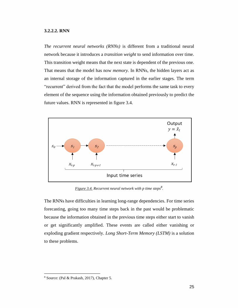
3.2.2.2. RNN
The recurrent neural networks (RNNs) is different from a traditional neural
network because it introduces a transition weight to send information over time.
This transition weight means that the next state is dependent of the previous one.
That means that the model has now memory. In RNNs, the hidden layers act as
an internal storage of the information captured in the earlier stages. The term
“recurrent” derived from the fact that the model performs the same task to every
element of the sequence using the information obtained previously to predict the
future values. RNN is represented in figure 3.4.
Figure 3.4. Recurrent neural network with p time steps8.
The RNNs have difficulties in learning long-range dependencies. For time series
forecasting, going too many time steps back in the past would be problematic
because the information obtained in the previous time steps either start to vanish
or get significantly amplified. These events are called either vanishing or
exploding gradient respectively. Long Short-Term Memory (LSTM) is a solution
to these problems.
8 Source: (Pal & Prakash, 2017), Chapter 5.
26
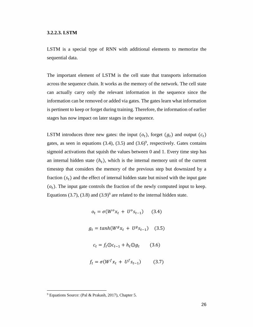
3.2.2.3. LSTM
LSTM is a special type of RNN with additional elements to memorize the
sequential data.
The important element of LSTM is the cell state that transports information
across the sequence chain. It works as the memory of the network. The cell state
can actually carry only the relevant information in the sequence since the
information can be removed or added via gates. The gates learn what information
is pertinent to keep or forget during training. Therefore, the information of earlier
stages has now impact on later stages in the sequence.
LSTM introduces three new gates: the input (𝑜𝑡), forget (𝑔𝑡) and output (𝑐𝑡)
gates, as seen in equations (3.4), (3.5) and (3.6)9, respectively. Gates contains
sigmoid activations that squish the values between 0 and 1. Every time step has
an internal hidden state (ℎ𝑡), which is the internal memory unit of the current
timestep that considers the memory of the previous step but downsized by a
fraction (𝑠𝑡) and the effect of internal hidden state but mixed with the input gate
(𝑜𝑡). The input gate controls the fraction of the newly computed input to keep.
Equations (3.7), (3.8) and (3.9)9 are related to the internal hidden state.
𝑜𝑡 = 𝜎(𝑊𝑜𝑥𝑡 + 𝑈𝑜𝑠𝑡−1) (3.4)
𝑔𝑡 = 𝑡𝑎𝑛ℎ(𝑊𝑔𝑥𝑡 + 𝑈𝑔𝑠𝑡−1) (3.5)
𝑐𝑡 = 𝑓𝑡⨀𝑐𝑡−1 + ℎ𝑡⨀𝑔𝑡 (3.6)
𝑓𝑡 = 𝜎(𝑊𝑓𝑥𝑡 + 𝑈𝑓𝑠𝑡−1) (3.7)
9 Equations Source: (Pal & Prakash, 2017), Chapter 5.

27
𝑠𝑡 = tanh(𝑐𝑡) ⨀𝑜𝑡 (3.8)
ℎ𝑡 = 𝑓𝑡 (3.9)
Now I will introduce briefly the functioning of each LSTM gate. Firstly, the
forget gate agrees to what information should be kept within the update to the
next step. The information from the previous hidden state and current input is
combined through a sigmoid function. Values come out between 0 and 1. The
closer to 0 means to forget, and the closer to 1 means to keep. Secondly, it is
necessary to pass the previous hidden state and current input gate into a sigmoid
function to transform values between 0 and 1, which means either not important
or important, respectively. Then it is also needed to pass the hidden state and
current input into the tanh function to squeeze values between -1 and 1. After
multiplying both outputs, the sigmoid output will decide which information is
important. At this moment, there are conditions to multiply the cell state by the
forget vector. This might drop some values if we multiply by values close to zero.
Then it takes the output from the input gate and do a pointwise addition to update
the cell state with the important information, which give us the new cell state.
Finally, the output gate decides what the next hidden state should be. The hidden
state contains information from the previous inputs. It is necessary to pass the
previous hidden state and current input into a sigmoid function and the modified
cell state to the tanh function. After we multiply both to decide what information
the hidden state will keep. The output is the hidden state. In detail, it is possible
to verify the LSTM structure in the figure 3.5. The gating mechanism of LSTM
allows memory transfer from over long-range timesteps.

28
Figure 3.5 – LSTM cell and its operations 10
10 Source: (Nguyen, 2018)

29
4. Data
The bitcoin price data11 (‘bprice’) ranges from “2017-06-18” to “2019-08-07” in
a daily period. The total number of observations is 781 (n=781). Note that I have
just considered historical data from the previous two years in order to remove
monotonic data from the initial bitcoin years. Since 2017, the bitcoin price has
become more volatile. On 13th October 2017 bitcoin price breaks the $5,000 for
the first time, on 28th November 2017 the $10,000 and on 18th December 2017
hits all time high just below $20,000. The bitcoin price time series can be
observed in figure 4.1. Non-linear trend and non-stationarity are the first
geometrical properties that can be highlight in figure 4.1.
Figure 4.1 - Bitcoin Price time series
I split the time series into train and test set by date “2019-04-01”, that is, the data
prior to this date is the training data and the data from this data onward is the
testing data. That means that we divide the sample into two subsets: 83.5% for
training (652 days) and 16.5% for testing (129 days). The data can be visualized
11 Coinbase, Coinbase Bitcoin [CBBTCUSD], retrieved from FRED, Federal Reserve Bank of
St. Louis; https://fred.stlouisfed.org/series/CBBTCUSD (accessed 11.08.2019).

30
once again in figure 4.2, where distinct colors (blue and orange) illustrates the
train test and the test sets.
Figure 4.2 - Bitcoin Price time series divided between training (blue) and testing (orange).

31
5. Models Implementation
In this chapter, I will implement the methods of both models described in chapter
3 in order to forecast the bitcoin price. All this analysis is developed using Python
software codes.
5.1. ARIMA
Firstly, I check the stationarity of the original time series in levels (with and
without trend) and the same for the first differences. For that, it will be used the
Augmented Dickey- Fuller (ADF)12 test. The results are described in the table
5.1.
Table 5.1- ADF test results. Computed by author from Python output.
(***), (**), (*) – rejection the null hypothesis at the 1%, 5% and 10% level respectively.
The critical values for each level can be checked in table 5.2.
Table 5.2- ADF critical values. Computed by author from Python output.
By analyzing the results from table 5.1, we conclude that the bitcoin price is non-
stationary at level (since we do not reject the null, that is, existence of a unit root),
12 Augmented Dickey- Fuller (ADF) test is used for testing the null hypothesis that a time series
is a unit root against the alternative hyphothesis that the time series is stationary (Pal & Prakash
,2017), Chapter 2.
Model Specification ADF statistic
Constant -0.219
Constant and trend -0.512
1st Differences -4.559 (***)
Model Specification 1% 5% 10%
Constant -3.439 -2.865 -2.569
Constant and trend -3.971 -3.416 -3.130
1st Differences -3.439 -2.865 -2.569

32
but stationary in the first-difference (since we reject the null of existence of a unit
root), comparing the ADF Statistic with all critical values from table 5.2
As mentioned previously, the well-known ARIMA (𝑝, 𝑑, 𝑞) defines the lag
observations in the auto-regressive part (𝑝), the number of times of differencing
(𝑑) and the size of moving average (𝑞). In the figure 5.1 and 5.2, it is possible to
analyze the ACF, PACF and the first differences of this time series, respectively.
From the analysis of the correlogram we observe that p=1 or p=2 will be the order
of the auto-regressive part of the ARIMA model.
Figure 5.1 - ACF and PACF function
Figure 5.2 – First differences
In order to select the best suitable ARIMA model, I used the AIC score for each
combination of 𝑝, 𝑑, 𝑞. The detail of each combination can be checked in the
table 5.3. In this particular case, the min AIC criteria states that the best suitable
model is the ARIMA (1,1,1).

33
No. p D q AIC
0 0 1 0 11,609.175
1 1 1 1 11,608.536*
2 1 1 0 11,610.824
3 0 1 1 11,610.812
4 2 1 1 11,609.803
5 2 1 2 11,612.258
Table 5.3- AIC score of different order ARIMA model. Computed by author from Python output.
*Best suitable model (lower AIC)
The results of ARIMA (1,1,1) are summarized in figure 5.3. Both first order auto-
regression (AR(1)) and moving average (MA(1)) processes are statistical
significant since their coefficients are different from zero, which can be
concluded by analyzing the associated p-values (are approximately zero, since
lower that any significance level).
Figure 5.3 - ARIMA (1,1,1) model results

34
The ARIMA (1,1,1) model is then used as the baseline forecasting model as the
results indicate.
Next, I will set in-sample lagged values for prediction. This model applies the
previous value to make the next prediction. In the figure 5.4, it is compared the
fitted and actual values for bitcoin prices ARIMA (1,1,1) forecasts that seem
closely good. However, due to the weaknesses of this model the predictions are
exactly coincident with one-lagged observations.
Figure 5.4 - ARIMA (1,1,1) forecasting. Forecasts (blue line) and bitcoin observations (orange
line).
In figure 5.5, it is represented the residuals plot for ARIMA predictions. This
figure compares the predict values of bitcoin price using ARIMA model (x-axis)
and their residual13 values (y-axis). The residuals get larger moving from left to
the right and there are few potential outliers, so there may be a few problems such
as heteroscedasticity14.
13 Difference between the observed value of the dependent variable (y) and the predicted value
(�̂�). 14 Systematic change in the spread of the residuals over the range of measured values.

35
Figure 5.5 – Residuals plot for ARIMA predictions
Note that in this case, I used the entire dataset for time series analysis. Ideally, I
would perform this analysis only on training dataset when developing the
predictive model.
Therefore, I will find the optimal ARIMA model using the out of time cross
validation. In order to do so, I split the time series into training and testing data,
83,5% and 16,5%, respectively. The results of ARIMA model forecasts can be
observed in figure 5.6. The model seems to give a directionally correct forecast.
However, the predicted forecasts are consistently below the actual observed
values.
Figure 5.6 - ARIMA (1,1,1) forecasting. Training data (blue line), testing data (orange line)
and forecasts (green line).

36
5.2. LSTM
In the previous section, I described a traditional model for time series analysis
(ARIMA) to forecast a series at a future point in time from observations taking
in the past. In this chapter, I will explore a method based on neural networks to
obtain the prediction of the same time interval as before. More specifically, I will
explore the Long Short-Term Memory (LSTM) model, which is a special
algorithm of Recurrent Neural Networks (RNN), able of learning long-term
dependencies.
For the specific case, I considered a total number of observations of 781 daily
bitcoin prices as previously. To be consistent with the ARIMA algorithm, I split
the dataset into 83,5% into training and 16,5% testing, respectively.
As a rule of thumb, whenever we use a neural network, you should normalize or
scale our data. I will use the Min-MaxScaler from sklear. preprocessing library
to scale data to a specific given range. In order to train LSTM, it is necessary to
convert our data into the shape accepted by the LSTM.
After converted our data into the desired format, it is time to create the LSTM
network architecture. The LSTM model will be a sequential model with multiple
layers. The sequential part allows us to create models layer-by-layer. It is limited
in the case that it does not allow to create models that share layers or have
multiple inputs or outputs. However, in our case, all layers have the same kind of
information.
The following step on the creation of the LSTM model is defining the layers in
the neural network. The time series-forecasting model has an input layer, which
feed into the LSTM layer and subsequently feed the output layer. The input layer
only specifies the sequence length that ranges between 1 and -1. For this
particular case, I defined a sequence length of 265. The LSTM layer has 160
neurons or nodes with a dropout layer (0,5) that randomly drops 50% of the input
before passing to the output layer, which has a single hidden neuron (dense layer

37
set to 1). I do not specify any batch size. Before start using the training data, it is
crucial to compile our LSTM. The details about the LSTM layers shape can be
checked in figure 5.7.
Figure 5.7 - LSTM layers shape.
Now is time to build the training model I defined in the previous few steps
with 𝑥_𝑡𝑟𝑎𝑖𝑛 𝑦_𝑡𝑟𝑎𝑖𝑛 as variables, 100 epochs and a validation split of 20%. The
cross-validation set is used to select the best performing algorithm. In this case,
I define to reduce the mean squared error loss function and to optimize with the
adam optimizer. The “val_loss” is the value of cost function for the cross-
validation data and “loss” is the value of cost function for training data.
In figure 5.8, it is possible to verify a decreasing value loss and loss function that
become almost stable after few epochs. After running the entire dataset few
times, the model starts to learn and minimize loss function.
Figure 5.8 - Value Loss and Loss Functions

38
Deep learning neural networks are trained using the stochastic gradient descent,
which is an optimization algorithm that estimates the error gradient for the
current state of the model from the training dataset, then updates the weights of
the model (“learning rate”) using the back-propagation of errors algorithm.
Thus, it is essential to rule the “learning rate” in the model. The learning rate is
a hyperparameter used in the training of neural networks which sets how quickly
the model is adapted to the problem. Smaller learning rates require more training
epochs given the smaller changes made to the weights each update. In this
particular case, I defined an automatic condition of optimizing the learning rate
at a specific positive number of epochs.
After setting LSTM model, I predict the bitcoin prices time series applying all
the parameters previously mentioned. In the figure 5.9 is compared the actual and
predicted values applying this model. This model seems to give quite good
forecasts of bitcoin prices with a smother version of observation values.
Figure 5.9 - LSTM forecasting. Observed values (orange line) and prediction values (blue line).

39
5.3 Results
The results demonstrate how LSTM and ARIMA models perform when
forecasting bitcoin prices. Each model predicts the bitcoin price in terms of its
forecasting error value for both RMSE and MAE.
MAE measures the average over the test sample of the absolute differences
between prediction and actual observations where all individual differences have
equal weight. RMSE is the square root of the average of squared differences
between prediction and actual observation. A lower value for both measures
implies better accuracy in prediction. Using 𝐹𝑡 as the forecast value, 𝐴𝑡 as the
actual value and n the number of time steps, the MAE and RMSE can be defined
as follows in equations (5.1) and (5.2)15.
𝑀𝐴𝐸 = ∑ |𝐴𝑡 − 𝐹𝑡 |𝑛
𝑡=1
𝑛 (5.1)
𝑅𝑀𝑆𝐸 = √∑ (𝐴𝑡 − 𝐹𝑡 )𝑛
𝑡=1
𝑛
2
(5.2)
RMSE using ARIMA and LSTM models is 4,725 and 361 respectively, yielding
an average of 4,364 reduction of errors achieved by LSTM. At the same time,
MAE shows a reduction of errors on average of 3.867 from ARIMA to LSTM
model. These results clearly indicate that LSTM model improved ARIMA
forecasts on average 92% and 94%, according to RMSE and MAE. The results
details can be observed in table 5.4.
Forecast RMSE %
Reduction
MAE %
Reduction
ARIMA LSTM ARIMA LSTM
Bitcoin
price
4,725 361 92% 4,106 239 94%
Table 5.4 - RMSE and MAE forecasting errors for both ARIMA and LSTM models.
Results printed via Python.
15 Equations source: (Elmasdotter & Nystrӧmer, 2018)

40
6. Conclusion
Machine learning techniques have recently gained a lot of popularity among the
international community. The main purpose of this dissertation was to know
whether these newly approaches are more powerful than the traditional methods,
or not. For this, I compared the accuracy of ARIMA versus LSTM forecasts for
a daily time-series of bitcoin prices.
For both models, I split the time series into training and testing data, 83.5% and
16.5%, respectively, in order to compare them. In the case of the ARIMA model,
the best suitable model was an ARIMA (1,1,1) using the min AIC criteria. This
model gives a correct direction forecast; however, the prediction values are
consistently below the real observations. In the case of the LSTM, I adjusted the
parameters of the model as follows: a sequence length of 265, a LSTM layer with
160 nodes, a dropout layer of 0.5, a dense layer set to 1, 100 periods and a
validation split of 20%. This model seems to give a quite good forecast with a
smoother curve than the actual observations.
The results show that LSTM predictions have better precision in terms of
forecasting errors: RMSE and MAE, they display on average an improvement of
92% and 94%, respectively, with respect to the ARIMA model. These results
confirm the literature insights, since the LSTM approach by large outperforms
the ARIMA output as previously mentioned.
Although this dissertation provides the expected results, some limitations should
be highlighted. Firstly, the data size is relatively short, and the LSTM algorithm
performs better in cases of longer time series. Secondly, bitcoin prices are not
seasonally adjusted. The time series of Bitcoin prices presents seasonality in
some months and even at the weekend users tend to make more transactions than
during week days. After removing seasonality, the time series would be cleaner,
and a higher forecasting performance would be obtained. Thirdly, daily data
creates more volatility to the series than one might have desired. Hence, weekly
data could be helpful to improve the accuracy of predictions as well.

41
A future extension of the analysis done in this dissertation could investigate the
performance of simpler versions of neural networks such as ANN. It would be
also interesting to forecast the bitcoin prices to few days in the future based on
historical past information. Alternatively, it could be also created a rolling
window model. These models focus on building a structure for time series
prediction that will divide the series in several windows. Huisu et al. (2018)
proved that the rolling window LSTM outperforms the normal LSTM in terms
of validation errors. Not least important, it would be worthy to include some
sentimental factors in the machine-learning optimization as previously
mentioned in chapter 2.2.
Even though the results were successful addressed, bitcoin prices should be very
difficult to predict due to its high volatility and inherently speculative behaviour.
As mentioned by Krugman (2018). “Bitcoin … whose price is almost purely
speculative, and hence incredibility volatile … Who’s driving the price now?
Nobody knows.” Even the most sophisticated machine-learning models will
always have a certain level of error due to this fundamental uncertainty around a
purely speculative variable.
Cryptocurrencies are here to stay for the next couple of years. If Bitcoin loses
reputation, other cryptocurrencies will emerge with better features. At the same
time, machine-learning models have still a long road ahead. There is still a great
potential to understand more precisely the behavior of bitcoin and other
cryptocurrencies prices.

42
7. References
Antonopoulos, A. M. 2014. Alternative Chains, Currencies and Applications,
Mastering Bitcoin: Unlocking Digital Cryptocurrencies, 219-233.
O’Reilly Media, Inc.
Athey, S., Parashkevov, I., Sarukkai, V., & Xia, J. 2016. Bitcoin Pricing,
Adoption, and Usage : Theory and Evidence. Working Paper No 17-033.
Stanford Institute for Economic Policy Research, Stanford.
Back, A., 1997. A partial hash collision based postage scheme
Barro, R. J. 1979. Money and the Price Level Under the Gold Standard. The
Economic Journal .89 (353): 13–33.
Böhme, R., Christin, N., Edelman, B. & Moore, T. 2015. Bitcoin: Economics,
Technology, and Governance. Journal of Economic Perspectives, 29(2),
213–238.
Box, G. and Jenkins, G. 1970. Time Series Analysis: Forecasting and Control.
Holden-Day, San Francisco.
Chaum, D., 1983. Blind signatures for untraceable payments. In: Chaum, D.,
Rivest, R.L., Sherman, A.T. (Eds.), Advances in Cryptology: Proceedings of
Crypto, vol. 82: 199-203. Springer.
Ciaian, P., Rajcaniova, M., & Kancs, d’Artis. 2015. The economics of BitCoin
price formation. Applied Economics, 48(19), 1799-1815.
Crosby, M., Nachiappan, Pattanayak, P., Verma, S. & Kalyanaraman, V. 2016.
Blockchain Technology: Beyond Bitcoin. Applied Innovation Review, (2),
5–20.
Dai, W., 1998. B-money, s.l.: s.n. Retrieved from:
http://www.weidai.com/bmoney.txt (accessed 10.08.2019).
Dyhrberg, A.H. 2015. Bitcoin, Gold and the Dollar – a GARCH Volatility
Analysis. Working Paper Series No. 15/20, University College Dublin,
UCD Centre for Economic Research, Dublin.
Elmasdotter, A., & Nystrӧmer, C. 2018. A comparative study between LSTM
and ARIMA for sales forecasting in retail. Unpublished thesis. KTH Royal
Institute of Technology, School of Electrical Engineering and Computer
Science, Stockholm.

43
Hochreiter, S. & Schmidhuber, J. 1997. Long Short-Term Memory. Neural
Computation. 9(8): 1735–1780.
Huisu, J., Ko, H., Lee, J. & Lee, W. 2018. Predicting Bitcoin Prices by Using
Rolling Window LSTM model. Paper presented at Data Science Festival
2018, London, UK.
Hyndman, R.J & Athanasopoulos, G. 2018 Forecasting: Principles and
Practice. Monash University, Australia: 2nd edn, Otexts.
Kingma, D & Ba, J. 2015. Adam: A Method for Stochastic Optimization.
Published as a conference paper at ICLR, 2015, San Diego, USA.
Krugman. P. 2018. Bubble, Bubble, Fraud and Trouble. The New York Times.
Nian, L & Lee, D. 2015. Introduction to Bitcoin. In. D. Lee (Eds). Handbook of
Digital Currency: Bitcoin, Innovation, Financial Instruments, and Big
Data. 5-29. Singapore: Elsevier.
Matta, M., Lunesu, I. & Marchesi, M. 2015. Bitcoin Spread Prediction Using
Social and Web Search Media. Unpublished dissertation, Università degli
Studi di Cagliari, Cagliari, Italy.
Mcnally, S. 2016. Predicting the price of Bitcoin using Machine Learning.
Paper presented at 26th Euromicro International Conference on Parallel,
Distributed and Network-based Processing (PDP 2018), Cambridge, UK.
Pal, D. A., & Prakash, D. P. 2017. Practical Time Series Analysis -Master Time
Series Data Processing, Visualization, and Modelling using Python.
Birmingham: Packt Publishing.
Nakamoto, S. 2008. Bitcoin: A Peer-to-Peer Electronic Cash System.
Schilling, L., & Uhlig, H. 2019. Some simple bitcoin economics. Journal of
Monetary Economics.
Schmidhuber, J., Gers, F.A. & Cummins, F. 1999. Learning to forget: Continual
prediction with LSTM. Presented at International Conference on Artificial
Neural Networks, Edinburgh, Scotland.
Shukla, N., & Fricklas, K. 2018. A peek into autoencoders. Machine Learning
with TensorFlow. Shelter Island, New York: Manning Publications Co.
Stiglitz, J. 2019. ‘We should shut down the cryptocurrencies.’ Retrieved from:
https://www.cnbc.com/2019/05/02/joseph-stiglitz-we-should-shutdown-
the-cryptocurrencies.html (accessed 26.08.2019).

44
Namin,S . S., & Namin, A. S. 2018. Forecasting Economics and Financial Time
Series: ARIMA vs. LSTM. Unpublished dissertation, Texas Tech
University, Texas, USA.
Nguyen, M. 2018. Ilustrated Guide to LSTM’s and GRU’s: A step by step
explanation. Retrieved from: https://towardsdatascience.com/illustrated-
guide-to-lstms-and-gru-s-a-step-by-step-explanation-44e9eb85bf21
(accessed 24.08.2019).
Reiff, N. 2019. Were there Cryptocurrencies before Bitcoin? Retrieved from:
https://www.investopedia.com/tech/were-there-cryptocurrencies-bitcoin/
(accessed 09.08.2019).
Stenqvist, E., & Lönnö, J. 2017. Predicting Bitcoin price fluctuation with
Twitter sentiment analysis. Unpublished thesis. KTH Royal Institute of
Technology, School of Electrical Engineering and Computer Science,
Stockholm.
Szabo, N., 2008. Bit gold, s.l.:s.n. Retrieved from:
http://unenumerated.blogspot.com/2005/12/bit-gold.html (accessed 10.08.2019).
Velde, F.R. (2013). Bitcoin: A primer. Chicago Fed Letter.
Yermarck, D. 2015. Is Bitcoin a Real Currency? An Economic Appraisal. In: D.
Lee (Eds). Handbook of Digital Currency: Bitcoin, Innovation, Financial
Instruments, and Big Data. 31-43. New York, USA: Elsevier.
Zhu, Y., Dickinson, D. & Li, J. 2017. Analysis on the influence factors of
Bitcoin’s price based on VEC model. Financial Innovation, 3:3
Zohar, A. 2015. Bitcoin: under the hood. The myths, the hype, and the true worth
of bitcoins. Communications of the Acm, 58(9).

45
8. Annexes
8.1 – ARIMA algorithm
1. # Necessary Packages
import numpy as np
import pandas as pd
import matplotlib.pyplot as plt
import statsmodels.api as sm
import statsmodels.formula.api as smf
from statsmodels.tsa.stattools import adfuller
from sklearn.metrics import mean_squared_error
from pandas import read_csv
from pandas import datetime
from pandas import DataFrame
from statsmodels.tsa.arima_model import ARIMA
from matplotlib import pyplot
2. # Bitcoin data
data1 = pd.read_csv('bitcoin.csv', header=0) # importing the bitcoin data
3. # visualize the data frame, first 10 elements
print(data1.head(10))
4. #graphical representation
data1.plot()
plt.show()
5. #read data again
series = read_csv('bitcoin.csv', header=0, index_col=0)
from statsmodels.graphics.tsaplots import acf, pacf
from statsmodels.graphics.tsaplots import plot_acf, plot_pacf
pyplot.figure()
pyplot.subplot(211)
plot_acf(series, ax=pyplot.gca(),lags=30)
pyplot.subplot(212)
plot_pacf(series, ax=pyplot.gca(),lags=30)
46
pyplot.show()
6. # returns or first difference of the time series
returns=series.diff()
returns.plot()
plt.show()
from statsmodels.tsa.arima_model import ARIMA
import pmdarima as pm
model = pm.auto_arima(series, start_p=1, start_q=1,
test='adf', # use adftest to find optimal 'd'
max_p=6, max_q=6, # maximum p and q
m=1, # frequency of series
d=None, # let model determine 'd'
seasonal=False, # No Seasonality
start_P=0,
D=0,
trace=True,
error_action='ignore',
suppress_warnings=True,
stepwise=True)
print(model.summary())
7. # fit an ARIMA model for the series
model = ARIMA (series, order=(1,1,1))
model_fit = model.fit(disp=0)
print(model_fit.summary())
8. # plot residual errors
residuals = DataFrame(model_fit.resid)
fig, ax = plt.subplots(1,2)
residuals.plot(title="Residuals", ax=ax[0])
residuals.plot(kind='kde', title='Density', ax=ax[1])
plt.show()
print(residuals.describe())

47
print(model_fit.aic)
9. # Actual vs Fitted
def forecast_accuracy(forecast, actual):
mape = np.mean(np.abs(forecast - actual)/np.abs(actual)) # MAPE
me = np.mean(forecast - actual) # ME
mae = np.mean(np.abs(forecast - actual)) # MAE
mpe = np.mean((forecast - actual)/actual) # MPE
rmse = np.mean((forecast - actual)**2)**.5 # RMSE
corr = np.corrcoef(forecast, actual)[0,1] # corr
mins = np.amin(np.hstack([forecast[:,None],
actual[:,None]]), axis=1)
maxs = np.amax(np.hstack([forecast[:,None],
actual[:,None]]), axis=1)
minmax = 1 - np.mean(mins/maxs) # minmax
#acf1 = acf(fc-test)[1] # ACF1
return({'mape':mape, 'me':me, 'mae': mae,
'mpe': mpe, 'rmse':rmse,
'corr':corr, 'minmax':minmax})
yy=model_fit.predict(652)
xx=series.iloc[652:781,0]
tt=forecast_accuracy(yy, xx)
print('forecast accuracy',tt)
pyplot.figure()
plt.scatter(xx,yy, marker='o')
pyplot.show()
pyplot.figure()
model_fit.plot_predict(652,781)
model_fit.plot_predict(dynamic=False)
pyplot.show()
10. # separate data in training and test data (95% and 5%)
forecast3, stderr, conf_int = model_fit.forecast(10)

48
print(forecast3)
pyplot.plot(forecast3,color='green')
pyplot.show()
pyplot.figure()
model_fit.plot_predict(752,791)
pyplot.show()
from math import sqrt
from sklearn.metrics import mean_squared_error
rms = sqrt(mean_squared_error(yy,xx))
print('RMSE', rms)
import numpy as np
import pandas as pd
import matplotlib.pyplot as plt
import statsmodels.api as sm
import statsmodels.formula.api as smf
from statsmodels.tsa.stattools import adfuller
from sklearn.metrics import mean_squared_error
from pandas import read_csv
from pandas import datetime
from pandas import DataFrame
from statsmodels.tsa.arima_model import ARIMA
from matplotlib import pyplot
from statsmodels.tsa.arima_model import ARIMA
from statsmodels.tsa.arima_model import ARMA
from statsmodels.tsa.seasonal import seasonal_decompose
11. # Bitcoin data
data = pd.read_csv('bitcoin.csv')
12. #divide into train and validation set
train = data[:int(0.835*(len(data)))]
valid = data[int(0.835*(len(data))):]
13. #preprocessing (since arima takes univariate series as input)

49
train.drop('Date',axis=1,inplace=True)
valid.drop('Date',axis=1,inplace=True)
14. #plotting the data
train['bprice'].plot()
valid['bprice'].plot()
15. #building the model
from pmdarima import auto_arima
model = auto_arima(train, trace=True, error_action='ignore',
suppress_warnings=True)
model.fit(train)
forecast = model.predict(n_periods=len(valid))
forecast = pd.DataFrame(forecast,index = valid.index,columns=['Prediction'])
16. #plot the predictions for validation set
pyplot.figure()
plt.figure(figsize=(10, 6))
plt.plot(train, label='Train')
plt.plot(valid, label='Valid')
plt.plot(forecast, label='Prediction')
plt.show()
17. #calculate rmse
from math import sqrt
from sklearn.metrics import mean_squared_error
from sklearn.metrics import mean_absolute_error
rms1 = sqrt(mean_squared_error(valid,forecast))
print('RMSE',rms1)
print('MAE', mean_absolute_error(valid, forecast))

50
8.2 – LSTM algorithm
1. # Loading the data and the preprocessing
import numpy as np
import pandas as pd
import matplotlib.pyplot as plt
import statsmodels.api as sm
import statsmodels.formula.api as smf
from statsmodels.tsa.stattools import adfuller
from sklearn.metrics import mean_squared_error
from pandas import read_csv
from pandas import datetime
from pandas import DataFrame
from statsmodels.tsa.arima_model import ARIMA
from matplotlib import pyplot
import seaborn as sns
from sklearn.model_selection import train_test_split
from sklearn.preprocessing import MinMaxScaler
from sklearn.metrics import mean_absolute_error
from sklearn.metrics import mean_squared_error
from sklearn.metrics import r2_score
from math import sqrt
2. # Bitcoin data
df = pd.read_csv('C:/Users/jmendes009/Desktop/Bitcoin/Python/Bitcoin-Price-
Forecasting-master/bitcoin.csv')
3. # visualize the data frame, first 10 elements
df['Date'] = pd.to_datetime(df['Date'])
df = df.set_index(['Date'], drop=True)
df.head(10)
4. #graphical representation
plt.figure(figsize=(10, 6))
plt.title('Bitcoin price')
51
df['bprice'].plot();
5. #We split the data to train and test set by date “2019–04–01” (that is,
the data prior to this date is the training data and the data from this data onward
is the test data, and we visualize it again).
split_date = pd.Timestamp('2019-04-1')
df = df['bprice']
trainf = df.loc[:split_date]
testf = df.loc[split_date:]
train2d = testf.values.reshape(-1,1)
test2d = testf.values.reshape(-1,1)
plt.figure(figsize=(10, 6))
ax = trainf.plot()
testf.plot(ax=ax)
plt.legend(['train', 'test'])
plt.title('Bitcoin Price train vs test')
plt.show()
plt.figure(figsize=(10, 6))
plt.title('Bitcoin Price test')
testf.plot();
plt.show()
prices = read_csv('bitcoin.csv', header=0, index_col=0)
prices.head()
seq_length = 265
minMax = MinMaxScaler()
X = minMax.fit_transform(prices)
X = X.squeeze()
x = []
y = []
for i in range(len(prices) - seq_length):
x.append(X[i: i+(seq_length)-1])
y.append(X[i+(seq_length)-1])

52
x = np.array(x)
y = np.array(y)
x_train, x_test, y_train, y_test= train_test_split(x, y)
print(x_train.shape)
print(x_test.shape)
print(y_test.shape)
print(y_train.shape)
x_train = x_train.reshape(-1, seq_length-1,1)
x_test = x_test.reshape(-1, seq_length-1,1)
6. # # Model building and training
import keras
from keras.layers import Input, LSTM, Activation, Dense
from keras.models import Sequential, Model
from keras.callbacks import LearningRateScheduler
model = Sequential()
input = Input((seq_length-1, 1))
X = LSTM(160, recurrent_dropout= 0.5)(input)
X = Dense(1)(X)
model = Model(input, X)
model.compile(loss='mse', optimizer='adam')
def reduce(epoch, lr):
if epoch%10 == 0:
return lr
return lr
scheduler = LearningRateScheduler(reduce)
history = model.fit(x_train, y_train, epochs=100, validation_split=0.2)
pyplot.figure()
plt.figure(figsize=(10, 6))
plt.plot(list(history.history['val_loss']))
plt.show()

53
pyplot.figure()
plt.figure(figsize=(10, 6))
plt.plot(list(history.history['loss']))
plt.show()
7. #Testing
predictions = model.predict(x_test)
from math import sqrt
rms1 = (sqrt(mean_squared_error(y_test, predictions)))
print('MAE1', mean_absolute_error(y_test, predictions))
print('RMSE1', rms1)
mape1 = np.mean(np.abs(predictions - y_test)/np.abs(y_test))
print('MAPE1', mape1)
pyplot.figure()
plt.figure(figsize=(10, 6))
plt.scatter(y_test,predictions, marker='o')
plt.show()
pred = minMax.inverse_transform(predictions)
#y_test=y_test.reshape(-1,1)
pred = pred.squeeze()
8. # test loss using mean absolute error
from sklearn.metrics import mean_absolute_error
from sklearn.metrics import mean_squared_error
from sklearn.metrics import r2_score
from math import sqrt
y1_test=minMax.inverse_transform(y_test.reshape(-1,1))
y1_test=y1_test.squeeze()
rms = (sqrt(mean_squared_error(y1_test, pred)))
print('MAE',mean_absolute_error(y1_test, pred))
print('RMSE', rms)
mape = np.mean(np.abs(pred - y1_test)/np.abs(y1_test))
print('MAPE', mape)

54
corr = (np.corrcoef(pred, y1_test)[0,1])
print('Corr' , corr)
#print(y1_test-pred)
mean=np.mean(y1_test)
print('mean', mean)
pyplot.figure()
plt.figure(figsize=(10, 6))
plt.scatter(y1_test,pred, marker='o')
plt.show()
pyplot.figure()
plt.figure(figsize=(10, 6))
plt.plot(y1_test)
plt.plot(pred)
plt.show()
9. # plotting subset from the data
pyplot.figure()
plt.figure(figsize=(10, 6))
p = model.predict(x[387:516].reshape(-1, seq_length-1, 1))
p = minMax.inverse_transform(p)
p = p.squeeze()
plt.plot(p)
plt.plot(minMax.inverse_transform(y[387:516].reshape(1,-1)).squeeze())
plt.show()
10. # ploting data of the past 2 years
pyplot.figure()
plt.figure(figsize=(10, 6))
p = model.predict(x.reshape(-1, seq_length-1, 1))
p = minMax.inverse_transform(p)
p = p.squeeze()
pyplot.figure()
plt.figure(figsize=(10, 6))

55
plt.plot(p)
plt.plot(minMax.inverse_transform(y.reshape(-1,1)).squeeze())
plt.show()