atmosphere

Article

Forecasting the Impacts of Prescribed Firesfor Dynamic Air Quality Management

M. Talat Odman 1,* ID , Ran Huang 1 ID , Aditya A. Pophale 1, Rushabh D. Sakhpara 1,Yongtao Hu 1, Armistead G. Russell 1 and Michael E. Chang 2 ID

1 School of Civil and Environmental Engineering, Georgia Institute of Technology, Atlanta, GA 30332, USA;ranhuang2014@gatech.edu (R.H.); aditya.pophale@gmail.com (A.A.P.);rushabh.sakhpara@gmail.com (R.D.S.); yongtao.hu@gmail.com (Y.H.); ted.russell@gatech.edu (A.G.R.)

2 Brook Byers Institute for Sustainable Systems, Georgia Institute of Technology, Atlanta, GA 30332, USA;chang@gatech.edu

* Correspondence: odman@gatech.edu; Tel.: +1-404-894-2783

Received: 21 April 2018; Accepted: 31 May 2018; Published: 8 June 2018�����������������

Abstract: Prescribed burning (PB) is practiced throughout the USA, most extensively in thesoutheast, for the purpose of maintaining and improving the ecosystem and reducing wildfirerisk. However, PB emissions contribute significantly to trace gas and particulate matter loads in theatmosphere. In places where air quality is already stressed by other anthropogenic emissions, PB canlead to major health and environmental problems. We developed a PB impact forecasting system tofacilitate the dynamic management of air quality by modulating PB activity. In our system, a newdecision tree model predicts burn activity based on the weather forecast and historic burning patterns.Emission estimates for the forecast burn activity are input into an air quality model, and simulationsare performed to forecast the air quality impacts of the burns on trace gas and particulate matterconcentrations. An evaluation of the forecasts for two consecutive burn seasons (2015 and 2016)showed that the modeling system has promising forecasting skills that can be further improvedwith refinements in burn area and plume rise estimates. Since 2017, air quality and burn impactforecasts are being produced daily with the ultimate goal of incorporating them into the managementof PB operations.

Keywords: burn activity forecasting; burn area; fire emissions; classification and regression tree (CART);community multiscale air quality (CMAQ) model; decoupled direct method (DDM); forecast evaluation;PM2.5; prescribed burning; satellite detection

1. Introduction

Prescribed burning (PB) is the intentional, controlled burning of dead and live vegetationfor agricultural, land clearing, or silvicultural purposes, or simply to reduce the wildfire risk [1].Here, we are mostly interested in the PB of forested lands. Forests in Southeastern USA contain manyfire-adapted tree species that need fire to survive [2]. Fire restores nutrients to the soil, kills invasivespecies, controls insects and disease, improves wildlife habitat, and reduces the accumulation ofdebris on the forest floor. If left untreated, accumulated debris increases the chances of catastrophicwildfires that not only destroy forests but cause loss of life and property [3]. Due to these benefits,land managers prefer prescribed fire over other alternatives. In Southeastern USA, more than2 million ha are treated with prescribed fire each year, and Georgia is one of the leading states inPB with nearly 550,000 ha year−1 [4].

Smoke generated by prescribed fires can travel long distances and contribute to air qualityproblems in urban areas [5] and threaten human health [6,7]. With all the other sources being controlled

Atmosphere 2018, 9, 220; doi:10.3390/atmos9060220 www.mdpi.com/journal/atmosphere

Atmosphere 2018, 9, 220 2 of 20

heavily, prescribed fire has become the leading source of PM2.5 (particulate matter with an aerodynamicdiameter smaller than 2.5 µm) in Southeastern USA, with 250 Gg year−1 or 27% of the total emissions [8].Wildfires are expected to increase in the future as a result of the changing climate [9,10]. We can expecta similar increase in the use of prescribed fire as a measure to prevent wildfires. This will furtherincrease the burden of prescribed fire emissions on the air quality of the region.

Accepting PB as a desirable forestry practice but understanding its negative impacts on airquality brings the challenge of finding the best compromise between forestry and air quality interests.Static solutions, such as imposing a burn ban during certain times of the year when air quality istypically burdened (e.g., ozone season) may be too restrictive for forestry interests. Conversely,conducting burns during certain times of the year (e.g., growing season) without regard for air qualitymay be inadequate to air quality interests. A more acceptable solution for both interests may befound through dynamic air quality management (DAQM), a paradigm where new information isincorporated in decision-making as soon as it becomes available. DAQM can involve the adaptationto new data that becomes available, such as air pollution measurements or new emissions estimates,or changes in activity patterns. For example, instead of operating with the same official emissionsinventory for several years, updated inventories could be used for interim years. Perhaps the mostagile form of DAQM is the one based on forecasting. PB activity is closely related to weather, especiallyto rain and winds [11]. Therefore, the upcoming demand for burning can be predicted from theweather forecast. Similarly, air quality can be, and is being, predicted using the weather forecast.Knowledge of the day-to-day fluctuations in prescribed fire emissions according to burn demandpredictions can significantly improve the accuracy of air quality forecasts. A reliable forecastingsystem, including weather, burn activity, air quality and impacts of PB on air quality, could lead tocohesive PB and air quality management strategies. If the impacts of different emission sources areforecast, then appropriate control measures can be taken to reduce those impacts and achieve betterair quality [12]. PB is one emission source that can be controlled more easily than other sources sinceburn/no-burn decisions are made every day. Through the permitting systems already in place inseveral Southeastern states, burns can be restricted on imminent poor air quality days and encouragedwhen meteorological conditions are more favorable. The application of DAQM in this manner maylead to maximized burn capacity while minimizing the impacts on air quality. It can also help to reducethe risk of human exposure to high levels of fire smoke.

Current air quality forecasting systems are not equipped with the tools necessary for the dynamicmanagement of PB operations. Typically, prescribed fires are assumed to be county-wide area sourceswith emissions equal to the average of several past years. The day-specific emissions used in theforecasts are generated by taking the rolling average over a specified period of daily prescribed fireemissions in a particular county for the years included in the average [11]. For example, if the selectedaveraging period is +/− 7 days and the years included are 2011–2015, then for 15 April, all fires in thatcounty are averaged from 8 April to 22 April for 5 years between 2011 and 2015. Such averaging greatlyreduces the day-to-day variability compared to the actual prescribed fire emissions. It also smoothsout the fires spatially by averaging multiple years of fire emissions over each county. The result is morefrequent, but less intense, fires over larger spans, which is not appropriate for an air quality forecastingsystem to be used in dynamic management. The National Air Quality Forecasting Capability (NAQFC)handles wildfire emissions by tracking satellite-detected ongoing fires that last at least 24 h [13].Prescribed fires are typically of shorter duration; they burn out in a few hours after their detection.Therefore, prescribed fires cannot be tracked in the same manner as wildfires for air quality forecastingpurposes. Estimating prescribed fire emissions from satellites is also problematic as it has been shownthat satellites seriously underestimate the burn areas in Southeastern USA [4]. What is needed is a burnactivity and impact forecasting system that can provide information well in advance so that burns canbe managed through the existing permitting systems.

Using a decision tree, we built a model to forecast how much PB activity is going to occur,when and where in Georgia, based on weather and historic burning patterns. Classification and

Atmosphere 2018, 9, 220 3 of 20

regression trees are one of the simplest and easiest to interpret statistical learning methods thatcan be built to make a prediction for an observation from predictor variables. Since they split thepredictor space into segments that look like the branches of a tree, they are called tree models.In the past, classification and regression trees have been used in the air quality field for various otherpurposes. Examples include the generation of annual mean concentrations from short episodes [14],model evaluation [15,16], the prediction of peak ozone or PM2.5 episodes [17], and air pollutionepidemiology [18]. To our knowledge, this is the first time a decision tree has been used to forecastprescribed fire activity. We started using this burn activity model to forecast prescribed fire emissionsand their impacts on air quality using an air quality forecasting system.

In what follows, the burn activity forecasting decision tree model and the methods used forprescribed fire emissions estimation are described in detail. The air quality forecasting system and itsfire impact forecasting capability are reviewed. An evaluation of the burn activity forecasts during thetest operation in 2015 and the production operation in 2016 are presented. This evaluation includescomparisons to satellite observations and ground-based accounts of fires. The skill of the forecastingsystem in predicting PB impacts is evaluated by comparisons to smoke-induced peaks in observedpollutant levels at network monitors in 2016.

2. Methodology

In this section, the method used for burn activity forecasting is described in detail. Then, the emissionestimation method, the air quality forecasting system and its fire impact forecasting capability areoverviewed. Finally, the metrics used for the evaluation of the forecasts are defined.

2.1. Burn Activity Forecasting

To conduct safe and effective burns, the fuels must be dry enough to catch fire but not so dry thatthey burn uncontrollably. Similarly, the winds must be strong enough to spread the fire over the land tobe treated but not strong enough to carry the flames beyond the perimeter. Based on these guidelines,the weather forecast can be used to predict PB activity, at least on a burn/no-burn decision level.

In Georgia, according to the Prescribed Burning Act of 1992, a permit is required for the PB ofwoods, lands, marshes, or other flammable vegetation. The Georgia Forestry Commission (GFC) is theagency in charge of issuing permits and keeping permit records. The burn season for most sites inGA is from 1 October to 30 April of the next year. A burn ban goes into effect in 54 counties duringthe ozone season (1 May–30 September). We obtained permit record data from GFC for the years2010–2016. Considering the burn season restriction, we focused our analysis on the first four monthsof each calendar year. The database contains the date and time, location and area of the burn, alongwith other information such as the purpose of the burn and the contact information of the burner.While some permit records have coordinates of the burn location, non-standard addresses that cannotbe readily georeferenced are also common, but all records contain the county of the burn location;therefore, the spatial resolution of our analysis was set at the county level. GFC makes available dailyweather forecast as well as observed weather data in an archive for fire danger ratings on its website.We downloaded the data for the 2010–2016 period at 18 fire weather stations in Georgia from thiswebsite. Information on how to download the data can be found in Appendix A.

A preliminary analysis of the data revealed that weather plays an important role in the decision ofthe burner [11]. In general, burns were not attempted on rainy days, days following large rain eventsor during prolonged dry periods. Surface wind speeds were generally between 5 and 15 mph on thedays when most burns were conducted. These findings as well as a weather forecast can be used asa first indicator of upcoming burn activity. Analysis has also shown that the amount of acreage treatedby fire increases when weather conditions are more favorable for conducting safe and effective burns.This trend along with historic burning patterns employed by a list of likely burners can be used topredict the location and size of the burns. The more precise the prediction of PB activity and emissions,the more accurate the fire impact forecasting will be.

Atmosphere 2018, 9, 220 4 of 20

2.1.1. Burn Days

The response variable is data labeled with two classes–burn day or no-burn day–coded as a binaryvariable. When the total burn area in a county on a particular day was greater than 30 ha, it wasconsidered to be a burn day in that county and it was assigned a value of 1; otherwise it was a no-burnday and was given a value of 0. The 30-ha limit was determined from the distribution of daily totalburn areas by county and is approximately equal to the mean minus one standard deviation. A setof 21 variables from the fire danger rating data were selected as predictor variables. A detaileddescription of these variables can be found in Appendix A. Missing values, most commonly for windspeed, were replaced by the average of the available values in the dataset for that variable. Data forthe years 2010–2014 were used to train the model. Later, the model was evaluated using the data forJanuary–April 2015.

The Classification and Regression Tree (CART) is a classification method that constructs a decisiontree model using historical training samples which can then be used to classify new, unseen data.For the details of the algorithm, please see Appendix B. The CART classifier is a binary decision tree,which is constructed by splitting the learning data into two branches, recursively. An example ofa decision tree generated by CART and a graphical representation of the decision boundary are shownin Figures A1 and A2, respectively. CART selects the best predictors on its own, prioritizes them anddiscards the least important ones. CART is non-parametric, i.e., it does not make any assumptionsabout the statistical distribution of variables, unlike linear regression which has two parameters—slopeand intercept. CART can handle outliers that affect other models such as linear regression.

The decision tree classifier model was implemented in python programming language using theScikit-learn library [19]. Scikit-learn uses an optimized version of the CART algorithm. Informationgain between two nodes is selected as splitting criteria for growing the tree. This is calculated usinginformation entropy between the nodes as shown in Figure A3. The predictor variable which gives thehighest information gain is placed at the root node and this procedure continues recursively to growthe tree. If we let the decision tree grow until all of the samples are classified, then it may overfit thetraining data. An overfitted decision tree tends to address noise instead of the underlying relationship.Hence, we needed to specify and limit the depth to which the tree could grow. This is called “pruning”the tree. The optimal depth was determined by measuring the model’s performance on the evaluationdataset. Performance evaluation will be described in Section 2.4 below. The decision tree model wastrained with a range of depths, and the shallowest tree with the best forecasting performance wasselected. Because of pruning, some of the 21 variables included in training may have been excludedfrom the decision tree model.

Two types of models were trained: a statewide model and county-specific models. In the statewidemodel, one decision tree model was trained to forecast PB activity for the entire state. To train the model,burn permit data of the counties in which the 18 fire weather stations reside were used. A single trainingdataset was created by concatenating the fire weather data from the 18 stations and the corresponding burnpermit data. A single decision tree was then trained with this dataset. The depth of the tree was optimizedby the pruning methodology discussed above. Once the decision tree model was trained, every county inGeorgia (159 counties in total) was assigned a station near to it. Forecast fire danger data from each assignedstation was used to forecast PB activity for the corresponding county.

In the county-specific models, every county had its own optimal decision tree for forecastingPB activity. When assigning a fire weather station to a county, the following methodology was used:First, for every county, 18 optimal decision trees were trained using that county’s burn permit data,and each of the 18 fire weather stations’ data. The forecasting performances obtained from eachof these 18 models were noted. Further, the distances between the county and the 18 fire weatherstations were calculated. The nearest fire weather station did not always yield the best performance.We selected the station that produced the best forecasting performance among the nearby stations.The burn permit data in that county were then used along with the fire danger data observed at theassigned station to train the decision tree model. The depth of the tree was optimized by the pruning

Atmosphere 2018, 9, 220 5 of 20

methodology discussed above. This procedure was followed to build PB forecasting models for allof the 159 counties in Georgia. To forecast PB activity in a county, the forecast fire danger rating datafrom the assigned station were fed to the model customized for that county.

2.1.2. Burn Areas

Georgia is one of the most active states in applying PB in the USA. Using the fire weather forecastdata as input, the decision tree model forecasts whether it is going to be a burn day or not in a particularcounty. Once a burn day is forecast, the next step in the process of forecasting PB impacts on air qualityis estimating the size and the location of these burns. First, we determined the daily average total burnarea for each county. For the 2015 burning season, we used the statewide model, and we assigned theannual average daily burn area to a county for every burn day that was forecast. Since there is strongseasonality associated with the amount of PB, while implementing the county-specific models for the2016 burning season, we used monthly average daily burn areas. This approach led to more accuratemonthly total burn areas than using the annual average daily burn areas.

To characterize the sizes of the burns, we grouped the counties in Georgia into threecategories according to their burner type—single dominant, multiple large and various small burners(Appendix C)—and assigned them typical burn sizes of 120, 80, and 40 ha, respectively. By dividingthe county total burn area to the typical burn size assigned to the county, we determined the numberof burns and randomly distributed that many burns of typical size to the forested areas of that county.

2.2. PB Emission Estimation

Once the location and the size of the burns are forecast, the next step in PB impact prediction is theestimation of emissions from the burns. Emission estimation starts with estimation of the fuel load andfuel consumption. A detailed description of the procedure used for emission estimation can be foundin Davis et al. [20]. We currently use the Fuel Characteristic Classification System (FCCS) fuel-bed mapsto determine the fuel loads in burn locations assigned to each county. In the future, more up-to-datesatellite products can be used to estimate the fuel loads in each grid cell where the burns are located.As for the determination of the fuel moistures required for the calculation of fuel consumption, we usethe previous day’s fuel moistures reported by the statewide Fire Weather Network. In the future,these fuel moistures can be modified according to the weather forecast for the burn day. Emissions arecalculated by multiplying the forecast burn area with the fuel loads per unit area, the combustionefficiency and the emission factors (i.e., mass of PM2.5 and other pollutants emitted per unit mass offuel burned) for Southeastern fuels published by the US Forest Service [21].

Since most prescribed fires in the Southeastern US are low intensity fires [22], we assume thatthe plumes do not penetrate the free troposphere. The resulting emissions are currently mixed intothe planetary boundary layer (PBL) portion of a vertical column of 4 km × 4 km grid cells over theburn location. This procedure was designed after conducting a sensitivity study to understand theinfluence of the vertical distribution of emissions [23]. Figure 10 in Garcia-Menendez et al. [23] showsthat modeled PM2.5 concentrations at a receptor are not too sensitive to the vertical distribution of fireemissions below the PBL height.

2.3. Air Quality and PB Impact Modeling

We have expanded our air quality forecasting system, HiRes [15], to forecast the impacts of varioustypes of emission sources for dynamic management purposes [12]. Using the sensitivities calculated bythe decoupled direct method (DDM) [24] available in the Community Multiscale Air Quality (CMAQ)model (version 5.0.2), the impacts of PB emissions to the forecast ozone and PM2.5 concentrations arecalculated. The new system, HiRes2, which consists of the Weather Research and Forecasting model (WRF)(version 3.6) and CMAQ, has been operational since 1 January 2015. DDM requires a well-defined emissionsource for each sensitivity that it calculates, and additional sensitivity calculations significantly increase thecomputational burden. We treat all PB emissions in Georgia as a single source and calculate a single DDM

Atmosphere 2018, 9, 220 6 of 20

sensitivity to statewide PB. Additional DDM sensitivity calculations are required to determine the impactsof PB emissions from a specific fire district or county within the state.

The air quality and burn impact forecasts are reported daily via a website [25]. Figure 1 showsthe PM2.5 and PB impact forecasts for 9 March 2016 as an example of a high burn activity day.Exceedance of the 35 µg m−3 daily average PM2.5 standard is expected for the purple colored grid cellsin Figure 1a. The PB impacts shown in Figure 1b are responsible for the exceedances. With thisinformation, the amount of area permitted to be burned can be restricted to avoid the forecastexceedances. The website also contains numerical information for maximum PM2.5 concentrations andPB impacts in each county along with the forecast burn areas.

Figure 1. Illustration of HiRes2 daily forecast products: (a) 24-h average PM2.5 (particulate matterwith an aerodynamic diameter smaller than 2.5 µm) concentrations (µg m−3) on 9 March 2016 and;(b) on a different scale, the portion of PM2.5 associated with prescribed burns in Georgia USA.

2.4. Forecast Evaluation

Forecasts are evaluated as binary occurrences. The divide between a positive occurrence anda negative occurrence is determined based on certain criteria. For example, recall that we defineda burn day as a day with total burn area of 30 ha or more in a county. In this example, a true positive isa correctly predicted burn day, a false positive is an incorrectly predicted burn day and a false negativeis an incorrectly predicted no-burn day. True positives (tp), false positives (fp), and false negatives (fn)are counted and the following metrics are used in evaluating the forecast performance. Precision, p,is the measure of true positives from the total predicted positives:

p =tp

tp + f p. (1)

Recall, r, is the measure of true positives from the total observed positives:

r =tp

tp + f n. (2)

F1 score is the harmonic mean of precision and recall:

F1 =2 × p × r

p + r. (3)

Atmosphere 2018, 9, 220 7 of 20

True negatives (tn) or correctly predicted no-burn days are also important from an accuracy pointof view. Accuracy, a, measures the overall correctness of the model:

a =tp + tn

tp + f p + tn + f n. (4)

The number of no-burn days exceeds the number of burn days by a large margin, and since weare more interested in correctly predicting the burn days, accuracy can be a deceiving performancemeasure. A burn day forecast model can yield high accuracy even if it misses the majority of the burndays. On the other hand, the F1 score places more importance on the burn days, whether they arepredicted correctly or missed, or whether the model predicts false burn days; therefore, it is a betterperformance measure than the accuracy. However, the F1 score treats fp and fn equally while, in reality,those occurrences may have different consequences. A metric that weighs fp and fn according to theeconomic value of their consequences might be better suited for forecast evaluation and should beconsidered in the future.

3. Results

In this section, first, the burn activity forecasts during the test operation in 2015 and the productionoperation in 2016 are first evaluated. This evaluation includes comparisons to satellite observations andground-based accounts of fires. Then, the skill of the forecasting system in predicting PB impacts is evaluatedby comparisons to smoke-induced peaks in observed pollutant levels at network monitors in 2016.

3.1. Evaluation of Burn Day Forecasts

The statewide model was used for burn impact forecasting in 2015, while county-specific modelswere used in 2016. The 2015 burn day forecasts were repeated with the county-specific models, and theF1 scores calculated for each county were compared to those obtained with the statewide model.Using county-specific decision trees, burn day forecasting performance improved significantly for the2015 burning season, compared to the use of a single, statewide model (Figure 2).

Figure 2. January–April 2015 burn day forecast F1 scores by county for the (a) statewide and(b) county-specific decision tree models.

Atmosphere 2018, 9, 220 8 of 20

We used the Hazard Mapping System (HMS) Fire and Smoke Analyses by NOAA [26] forqualitative evaluation of our forecasts. Every day, we compared our burn forecasts to the dailyanalyses by NOAA and gave them a rating based on the agreement in regard to the location anddensity of the fires. Figure 3 shows an example where the rating was “excellent”. This subjective ratingwas given based on the agreement both in location and density of the fires between the forecast andthe analysis, everywhere except in Northeastern Georgia where the cloud cover may have obstructedthe satellite’s view. It should also be kept in mind that other factors, such as the forest canopy, can alsointerfere with the satellite retrieval. We used the highest impacts of the burns on PM2.5 concentrations(shown in purple in Figure 3b) as a proxy for the locations of the burns. Also, since the burn forecast isfor Georgia only, the fires observed in other states were ignored for the purposes of this evaluation.

Figure 3. (a) NOAA’s Hazard Mapping System Fire and Smoke Analysis; (b) forecast of burn impactson PM2.5 levels; and (c) cloud cover for 3 March 2016. The largest impacts on PM2.5 (shown in purple)can be used as a proxy for burn locations.

This qualitative evaluation is conducted as a first indication of the suitability of the burn forecast.Clearly, the ability to correctly predict the locations of the burns influences the accuracy of the fireimpact forecasts at specific air quality receptors. A “good” or better rating warrants more detailedanalysis, including qualitative evaluation. The number of good or better agreement days increased in2016 with the county-specific models compared to 2015 when the statewide model was used for PBimpact forecasting, especially in March when the burn activity peaked.

3.2. Evaluation of Burn Area Forecasts

By regressing forecast versus permitted daily total burn area statewide, we estimated the temporalaccuracy of the models in forecasting the PB area. Figure 4 shows the regression lines for boththe statewide and county-specific models. The coefficients of regression (slope and intercept) withmargins of error (using 95% confidence interval), the coefficient of determination (R2) and the standarderror of estimate (σ(y)) are also shown. Each data point in these scatter plots represents a dayfrom the January–April 2015 period. For both models, there are more points below the 1:1 lineindicating an overall underestimation of daily total burn areas. In general, small burn area totalswere overestimated while large totals were underestimated. This was more pronounced with thecounty-specific models which underestimated all burn totals above 7000 ha. The standard error ofestimate given by the county-specific models (2170 ha) was smaller than that of the statewide model(5070 ha); also, the R2 of regression was larger in the case of county-specific models (0.34) than that ofthe statewide model (0.11).

Atmosphere 2018, 9, 220 9 of 20

Figure 4. Forecast versus permitted daily total burn areas (ha) in Georgia for the January–April 2015period: (a) statewide model; and (b) county-specific models.

The regression of forecast versus permitted county total PB area over the season gave us an idea aboutthe spatial accuracy of the models in forecasting PB area. Figure 5 depicts the regression lines for both thestatewide and county-specific models. Each data point in these scatter plots represents a county. Once again,the burn areas were generally underestimated, the standard error of estimate given by the county-specificmodels (2150 ha) was smaller than that by the statewide model (2820 ha) and the R2 of regression was largerin the case of county-specific models (0.47) than that in the statewide model (0.29).

The slope and R2 values for the regressions of the county totals in Figure 5 were greater thanthose for the regressions of the daily totals in Figure 4. Further, both the intercepts of the lines andthe standard errors of the estimates were smaller for the county totals than those for the daily totals.Therefore, the overall spatial accuracy in forecasting the location of the burns at the county levelresolution was higher than the temporal accuracy in forecasting the day of the burns.

Figure 5. Forecast versus permitted county total burn areas (in ha) in Georgia for the January–April 2015period: (a) statewide model; and (b) county-specific models.

Atmosphere 2018, 9, 220 10 of 20

We expected similar performance for the burn area forecast in 2016. However, when we comparedour forecast burn areas to the permitted burn areas, we found that the underestimation in forecast burnareas was greater both in terms of daily statewide totals and county totals for the 2016 burn season(Figure 6). From January to April 2016, a total of 480,000 ha was permitted to be treated by PB while only200,000 ha was forecast. The correlation between forecast and permitted burn areas has also degradedcompared to 2015. In contrast to 2015, the spatial accuracy in forecasting the burns in each county wasworse than the temporal accuracy in forecasting the day of the burns. These changes in the performanceof the burn area forecast were most likely because of the El Niño–Southern Oscillation (ENSO) andthe La Niña conditions of 2015–2016 that created very different precipitation patterns in SoutheasternUSA during the 2016 burning season compared to the 2010–2014 period. The temperatures during themonth of March, at the peak of PB activity, were much above average and precipitation was belowaverage (www.ncdc.noaa.gov/temp-and-precip).

Burn areas in permit records during the first four months of 2016 increased by 20%, from 400,000 ha in2015 to 480,000 ha in 2016. This may have played a significant role in the underestimation of the daily totalburn areas that were being forecast based on 2010–2014 averages, supporting the role of atypical weatherduring the first four months of 2016. Despite the overall underestimation of burn areas, there were stilla large number of days and counties where burn areas were overestimated. In Figure 6, these are the pointsremaining above the 1:1 line, and for almost all of them, the permitted burn areas are below 4000 ha.

Figure 6. Forecast from county-specific models versus permitted (a) daily total burn areas in Georgia;and (b) county total burn areas for the January–April 2016 period.

3.3. Evaluation of Burn Impact Forecasts

The overall statistics of the 2016 burn impact forecasts are shown in Figure 7. If the maximumafternoon PM2.5 concentration on a particular day is in the 95th percentile of all observed afternoonmaximum concentrations during the burn season, then that monitor is most likely impacted byPB. To be sure, burn permits in the county in which the monitor resides as well as the countiessurrounding the monitor were reviewed to see if there were any permitted burns that may have affectedthe observations on that day. The 95th percentile of all observed afternoon PM2.5 concentrationswas 32 µg m−3. On the other hand, the 95th percentile of all forecast maximum afternoon PM2.5

concentrations was 43 µg m−3. The common threshold for forecast evaluation was set at 32 µg m−3

as shown in Figure 7. The precision, recall and F1 score for correctly predicting the PB impacts over32 µg m−3 were equal to 19%, 36%, and 25%, respectively.

Atmosphere 2018, 9, 220 11 of 20

Figure 7. The 2016 burn impact forecast statistics. The thresholds for burn impacts are drawn at32 µg m−3, which is the 95th percentile of all observed maximum afternoon PM2.5 concentrationsthroughout Georgia between 2 January and 1 May 2016.

The number of false positives is approximately three times as large as the number of falsenegatives in Figure 7, which indicates a general overestimation of the burn impacts. This may be,in part, due to the overestimation of the burn areas for low burn activity and underestimation forhigh burn activity days. To investigate other possible reasons, we focused on the true positives inFigure 7 and analyzed the relationship between the bias in burn impacts and the bias in burn areas.For the true positives that were associated with the PM2.5 monitors in Albany (Daugherty County)and Augusta (Richmond County), Georgia, we calculated the burn areas in the county where themonitor resides and in the immediate upwind county (or counties depending on wind direction).The difference between the forecast and permitted burn areas were normalized by the permitted burnarea and plotted on the x-axis in Figure 8. Note that the burn areas were underestimated with theexception of one day, 24 January 2016, in Daugherty County and its upwind county. The differencebetween the forecast and observed afternoon maximum PM2.5 concentrations were normalized bythe observed concentration and are plotted on the y-axis in Figure 8. The strong correlation betweenthe two biases (R2 = 0.77) suggests that the overestimation of the burn impact may be related to anoverestimation of the emissions, because the emissions are proportional to burn area. The slope ofthe linear regression line suggests that this emission overestimation may be around 47% (±23%).The reason for this overestimation may be either an overestimation of the fuel consumption or highbiased emission factors. The large intercept (0.96 ± 0.16) indicates that there must have been anotherfactor that was not emission related. One potential reason is plume dispersion. The fraction of theactual smoke plumes penetrating into the free troposphere may have been larger than the fraction inour forecasts, which we assumed to be zero, leading to an overestimation of the ground-level PM2.5

concentrations at the observation sites.

Atmosphere 2018, 9, 220 12 of 20

Figure 8. Normalized bias in PM2.5 versus normalized bias in burn areas in upwind counties. The burnareas were generally underestimated. Independent from the bias in burn areas, the PM2.5 impacts weremostly overestimated.

4. Discussion

We have developed, to the best of our knowledge, the first dynamic PB impact forecasting system.While previous air quality forecasting systems used prior year averages of PB emissions, this system predictsthe PB activity and calculates corresponding PB emissions based on the weather forecast. It predictedactive burn days at a county scale with an F1 score larger than 0.50 over most of the Lower Piedmont andCoastal Plain regions of Georgia where more lands are treated with prescribed fire than the rest of the state.The PB forecast overestimated the burn areas on less active burn days while underestimating them on moreactive days. This may be due to using monthly average burn areas in the forecast whereas actual burnareas vary more frequently due to some days being more conducive to burns than others, as well as therandom behavior of the burners. The number of correctly predicted significant smoke impacts at downwindreceptors (PM2.5 concentration larger than 32 µg m−3) was about six times smaller than the total number ofmisses and false alarms. However, there was a very strong correlation between the bias in smoke impactsand the bias in burn areas. Therefore, if the bias in forecast burn areas can be reduced, the skill in predictingsmoke at downwind receptors will be greatly improved.

The current skill of the forecasting system and its potential for improvement opens new avenuesfor dynamic air quality and cohesive PB management. For example, the forecasting system couldbe used as a decision support tool, as follows. In Georgia, where a permit is required by law for PB,land managers call the GFC district offices, typically early in the morning, to obtain a permit for a burnlater that day. The burn activity and burn impact forecasts provided by our forecasting system could beused by GFC to manage prescribed burns to avoid any potential exceedances through their permittingsystem. For example, on the morning of 18 January 2016, GFC offices could see on our website that thedaily average PM2.5 concentrations in Thomson County would be as high as 75 µg m−3, with 70 µg m−3

coming from burns throughout Georgia, including 560 ha in Thomas County. Assuming the PB impactis solely from burns in Thomas County, our forecast suggests that each hectare burned will contribute0.125 µg m−3 to the PM2.5 concentration. Therefore, to avoid exceeding the national ambient air qualitystandard (NAAQS) of 35 µg m−3 for daily average PM2.5, permits in Thomas County should be limitedto 240 ha that day. In fact, considering potential contributions from upwind counties, the limit shouldbe set below 240 ha. Clearly, it would be more useful to forecast exactly how many hectares can beburned in each county without violating any air quality standards.

Atmosphere 2018, 9, 220 13 of 20

Our current impact forecast considers all burns in the state without distinction of local versusdistant burns. Calculating the impacts of burns separately for every county by applying DDM toemissions from 159 counties in Georgia is computationally very demanding. Future research shouldfocus on finding efficient ways of partitioning the total impact calculated by DDM into impacts ofthe individual counties or, better yet, individual burns upwind. If the PB impact can be brokendown by specific burns, it will be seen that some burns contribute little to air quality and exposurewhile others contribute more. With information on the marginal contribution of each burn to the airquality downwind, the following dynamic management protocol can be employed. The burns thathave minimal impact will, therefore, be permissible, while the ones that contribute a lot may haveto be denied. For example, suppose burn A contributes almost nothing to the regional peak PM2.5

concentration. Burn B contributes a little bit more, but still not very much. Burn C contributes stillmore, and so on, say up through to burn Z. If all burns, A–Z, were permitted, then the region mightexceed the NAAQS. However, there might be a point where PM2.5 concentrations would stop short ofthe NAAQS, say when only burns A–N were permitted. This approach might maximize the amount ofland that could be burned without going over the NAAQS. Burning any more (i.e., burns M–Z) wouldput the region over the NAAQS, so those burns have to be left to another day. Currently, there is a burnban that goes into effect on 1 May in 54 counties due to the ozone season. However, there is interest inburning in May and June, and our forecasting system could identify windows of opportunity duringthose months. Burners that were denied earlier could be encouraged to burn during this period.

Because our burn activity forecast is the first of its kind and integrates several ad hoc elements, the burnimpact forecasting system has a lot of room for improvement. One area where significant improvementscan be made is the assignment of daily burn areas. Using monthly averages instead of an annual averagewhen assigning daily burn areas to each county improved the performance of the burn forecast because ofthe large variation in burn activity throughout the year. However, the skewness of the burn area distributionsuggests that even a monthly average may not be appropriate for capturing the variation. Recall that withmonthly averages, we still underestimated high burn activity while overestimating lower activity, leading tolow slopes of linear regression lines compared to 1:1 lines. A better approach may be to regress the countytotal daily burn areas with the same predictors that we currently use for burn/no-burn day classification.The binary decision is not able to capture varying degrees of favorable burn conditions. The burn areas underexcellent burn conditions might be much larger than those under marginal conditions. A regression model isbetter suited than a classification model for covering the spectrum of favorable conditions and associated burnactivity. When a sufficient amount of training data becomes available, a regression model should be tested.Also, other approaches such as the random forest model [27] could be tested in the future. Another area ofpossible improvement is the designation of burn locations within the county. By keeping track of prior permitsissued and comparing them to historic burning patterns of individual burners (e.g., burn sizes, frequency,and time of the year), the demand for burning could be forecast more accurately. This may reduce, to a greatextent, the need for random assignment of forecast burns to managed lands. Also, by tracking who is mostlikely to burn and where, accurate burn sizes could be forecast instead of the typical burn sizes that arecurrently fixed at 120, 80 or 40 ha according to the dominant burner type in each county.

Aside from the overestimation of burn areas for low burn activity days, uncertainties inemissions and plume heights may be among the reasons for overestimation of the burn impacts,i.e., the false positives in our forecasts. In addition, it is well known that air quality models like CMAQtypically dilute the plumes, leading to underestimation of the local impacts. Therefore, the rates ofoverestimation in emissions and/or underestimation of the plume heights may be more severe thanour analysis suggests. Our current approach for injecting PB plumes in the vertical layers of CMAQ isbased on the assumption that most prescribed burns in Southeastern USA are low intensity fires whoseplumes do not penetrate the free troposphere. A better approach would be to estimate the plumeheight from the heat of combustion and to split the emissions between the boundary layer and thefree troposphere. Beginning in 2017, we started using the plume height algorithm of Liu [28], which isbased upon regressions of measured plume heights with weather-related parameters.

Atmosphere 2018, 9, 220 14 of 20

Following the development and evaluation of the fire impact forecasting system, we havecontinued to forecast burn activity and burn impacts on a daily basis since the beginning of 2017.These forecasts are posted regularly to our website for the benefit of regulatory agencies. We developeda protocol for incorporating the air quality and impact forecasts into the current PB permitting processin Georgia. The protocol involves denying applications or restricting the sizes of the permits on poor airquality days and encouraging burns on days when there are no imminent air quality concerns. We arefocusing our research efforts on expanding our forecasts to predict the burn impacts by county andeventually, by individual burns. We are also extending our forecasts to other states in Southeastern USA.Not all states have permit records that are as comprehensive as those of Georgia. For those states, we aredeveloping fire activity forecasts based on satellite fire detections. Although current satellites severelyunderestimate the burn areas of small, prescribed fires [4], we are hopeful that reliable burn impactforecasting will be possible with the increased spatiotemporal resolution of next generation satellites.

5. Conclusions

An analysis of the GFC burn permit database for the years 2010–2014 revealed that the season andweather play important roles in the burn/no-burn decisions made by land managers. Acreage treatedby fire increases in February and March and when weather conditions are more favorable forconducting safe and effective burns. This triggered the idea of forecasting burn activity based onthe time of the year and the weather forecast. A PB activity forecasting model was developedusing the CART method with the daily burn areas by county from GFC’s burn permit database andmeteorological parameters from the closest fire weather monitors. The number of predictor variableswas limited to circumvent over-modeling. The model was trained with statewide data for the years2010–2014 and evaluated with 2015 data. Four metrics were used for evaluation: (1) the accuracy or theoverall correctness of the model; (2) the precision or the accuracy in predicting burn days; (3) the recallor the number of correctly predicted burn days over the number of burn days; and (4) the F1 score,which is the harmonic mean of precision and recall. Later, considering the geographic variation inthe demand for burning, this statewide model was replaced with county-specific models (a differentmodel for each of the 159 counties in Georgia). The F1 score of the burn forecasts for 2015 improvedsignificantly with the county-specific models, showing their clear advantage over a single modelfor the entire state. In addition, because of the strong seasonality associated with the amount of PB,we started to employ different daily average burn areas for each month, instead of one average for theentire burn season.

If the burn-forecast model predicts a burn day, the daily average burn area for the county issplit into burns of typical size, which are distributed randomly to forested areas. Then, the amountof fuel that these burns would consume is estimated using FCCS fuel load maps and fuel moisturedata from the fire weather network. Fire emissions are then calculated using emission factors that arecharacteristic of Southeastern fuels and inpu‘t to the HiRes2 air quality forecasting system. HiRes2provides forecasts of not only air quality (O3 and PM2.5) but also impacts of PB on air quality, using theDDM sensitivity analysis method.

The forecasting skills of the PB impact prediction system were evaluated for the 2015 and 2016burn seasons (January–April). The burn forecasts were evaluated qualitatively every day against theNOAA HMS Fire and Smoke Analyses for agreement in regard to the location and density of thefires, and quantitatively, at the end of the burn season, against burn areas permitted by GFC. In 2015,the correlation between the predicted and permitted daily statewide total burn areas was stronger withthe county-specific models than with the statewide model. However, even with the better performingcounty-specific models, both the daily statewide total and the countywide seasonal total burn areaswere generally underestimated, with some overestimations for low burn activity days or countiesand large underestimations for high activity days or counties. In 2016, the underestimation was moresevere than in 2015, probably due to the ENSO conditions at the beginning of the year.

Atmosphere 2018, 9, 220 15 of 20

Burn impact forecasts were evaluated using observations of possible PB impacts by the statewideair quality monitoring network. In 2016, the precision, recall and F1 score for correctly predictingthe PB impacts over 32 µg m−3 (the 95th percentile of all observed afternoon PM2.5 concentrations atGeorgia’s PM2.5 monitors in 2016) were equal to 19%, 36%, and 25%, respectively. An analysis of thecorrelation between forecast biases showed that the bias in burn impact forecast could be reducedif the burn area forecast was improved. The unexplained portion of the bias is probably due to theuncertainty in fire emissions and/or the plume rise treatment in the modeling system, which, prior to2017, assumed no penetration into the free troposphere.

Author Contributions: M.T.O. and M.E.C. conceived the idea of prescribed fire impact forecasting for dynamic airquality management. M.T.O. designed the forecasting system, directed the research and wrote the paper. A.G.R.provided guidance and contributed to the analysis of the data. R.D.S. and A.A.P. contributed to the developmentof the decision tree model for burn activity forecasting. Y.H. integrated the modeling system and conducted theforecasting operation. A.A.P. and R.H. contributed to the evaluation of the burn activity and burn impact forecastsand to the writing of the paper.

Funding: This research was funded by the National Aeronautics and Space Administration (NASA) AppliedSciences Program grant numbers NNX11AI55G and NNX16AQ29G, U.S. Environmental Protection Agency Scienceto Achieve Results Program grant number RD8352170, and the Joint Fire Science Program of U.S. Department ofthe Interior and U.S. Forest Service grant number 16-1-08-1. The costs to publish in open access are covered byNASA grant number NNX16AQ29G.

Acknowledgments: The contents of the publication are solely the responsibility of the grantee and do notnecessarily represent the official views of the supporting agencies. Further, The USA Government does notendorse the purchase of any commercial products or services mentioned in the publication. We thank DanielChan and Frank Sorrels of Georgia Forestry Commission for providing the Georgia prescribed burn permit data.

Conflicts of Interest: The authors declare no conflict of interest. The funding sponsors had no role in the designof the study; in the collection, analyses, or interpretation of data; in the writing of the manuscript, and in thedecision to publish the results.

Appendix A

We obtained the fire danger rating data for the 2010–2016 period, available for 18 fire weatherstations in Georgia, from http://weather.gfc.state.ga.us/SearchPrompt.aspx. By selecting Fire DangerRating under Type of Forecast, one can obtain the observed fire danger rating data at all stations fora desired month. Twenty-one variables from the fire danger rating data were used as predictorvariables (Table A1). The values are observed values at the stations at 1 p.m. EST.

Table A1. Dataset of variables in fire danger rating.

No. Variable Description Units

1 Temp Temperature F2 RH Relative humidity %3 Wind Wind speed and direction Mph4 Mx_Wind Maximum wind speed Mph5 Dur Duration of rainfall Hours6 Rn24 Rainfall amount in the last 24 h Inches

7 SoW

State of weather coded as:0. Clear, less than 1/10 cloud cover1. Scattered clouds, 1/10–5/10 cloud cover2. Broken clouds, 6/10–9/10 cloud cover3. Overcast, 10/10 cloud cover4. Fog5. Drizzle6. Rain7. Snow or Sleet8. Showers9. Thunderstorm

8 Scode

Season code:1. Winter2. Spring3. Summer4. Fall

Atmosphere 2018, 9, 220 16 of 20

Table A1. Cont.

No. Variable Description Units

9 KBDIKeetch–Byram Drought Index (KBDI) measures moisture in deep duffs or uppersoil layers. The relative dryness of soil is important in fire suppression. KBDIvaries from 0 (wet) to 800 (dry).

10 Tmax Maximum temperature in the last 24 h F11 Tmin Minimum temperature in the last 24 h F12 RHMax Maximum relative humidity in the last 24 h %13 RHMin Minimum relative humidity in the last 24 h %

14 HrbGFHerbaceous greenup factor (HGF): the actual greening and curing of liveherbaceous vegetation. HGF varies from 0 (completely cured) to 20 (completelygreen).

15 WdyGFWoody greenup factor (WGF): this expresses the actual greening and curing oflive woody vegetation. WGF varies from 0 (completely cured) to 20 (completelygreen).

16 Herba-ceous Fuel moisture in live herbaceous vegetation. %17 Woody Fuel moisture in live woody vegetation. %18 SC Spread component: this is the forward rate of spread at the head of the fire. ft min−1

19 EC Energy release component: this is the potential available energy per unit area atthe head of the fire.

BTUft−2.

20 BI Burning index (BI): dividing BI by 10 gives a reasonable estimate of the flamelength in feet at the head of a fire. BI is fuel model dependent factor.

21 Class Day

Class of day, describing the potential for wildland fires, coded as:1. Low2. Moderate3. Very high4. Extreme

Appendix B

A detailed description of the CART algorithm can be found in Breiman et al. [29]. Here, we willhighlight its principal elements.

The root node in Figure A1 includes all of the training samples to start with. The training samplesare then partitioned by decision boundaries using predictor variables—variable 1 and variable 2 here(Figure A2). Each node of the tree, except for the terminal node, represents a conditional question tothe predictor data. If the value of a predictor is greater than a certain value, then the left branch ofthe tree is chosen; otherwise the right branch is chosen. If we keep doing this at every node, we reacha terminal node where we obtain the probabilities for each class. Pi,j,k is the probability of class i atlevel j and node k. If the probability for a class is greater than a defined threshold value (generally 0.5)then we make the forecast for that class: ‘burn day’ or ‘no-burn day’.

Figure A1. An example decision tree to generate the forecasting probabilities of each class.

Atmosphere 2018, 9, 220 17 of 20

Figure A2. Decision boundaries created by the Classification and Regression Tree (CART) algorithm toclassify the data using variable 1 and variable 2.

The information gain between two nodes is calculated using the information entropy between thenodes, as shown in Figure A3. For simplicity, only the probability index for class is retained in Figure A3.

Figure A3. Information gain calculations.

Atmosphere 2018, 9, 220 18 of 20

The information gain, g, in this example is equal to

g = 0.811 − 1320

× 0.719 − 720

× 0.863 = 0.041 . (A1)

The predictor variable which gives the highest information gain (highest reduction in impurity) isnaturally placed at the root node, and this procedure continues recursively to grow the tree.

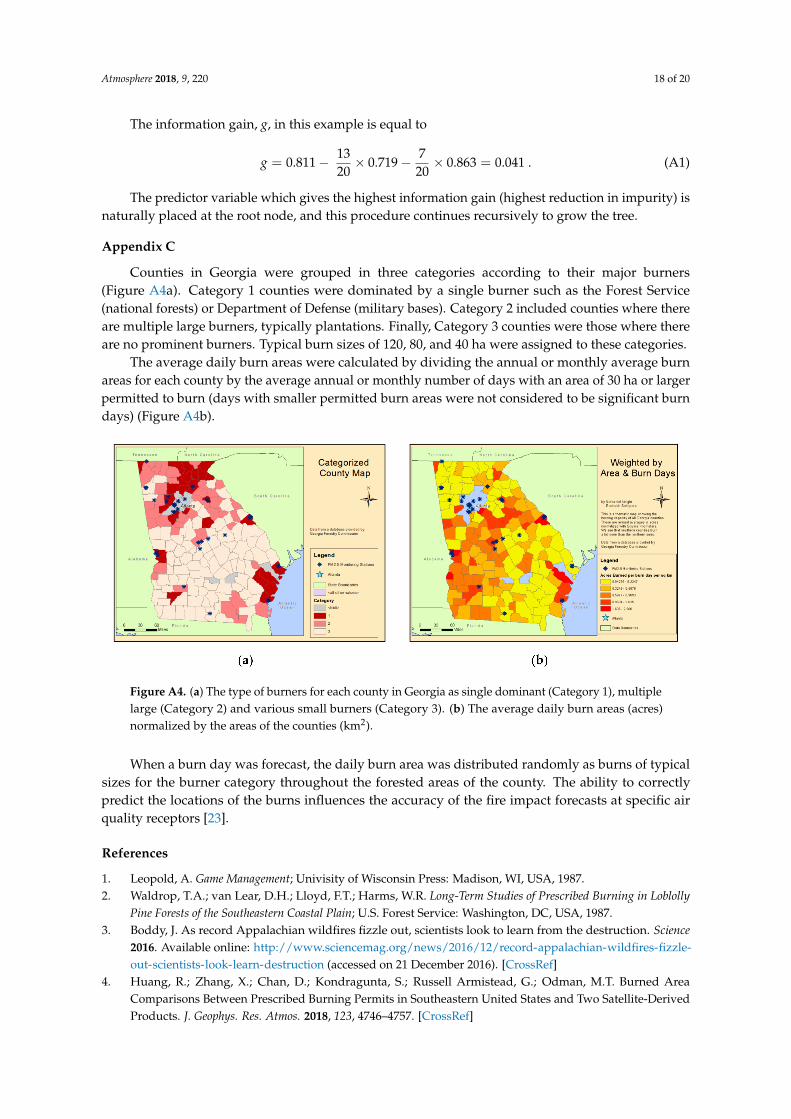
Appendix C

Counties in Georgia were grouped in three categories according to their major burners(Figure A4a). Category 1 counties were dominated by a single burner such as the Forest Service(national forests) or Department of Defense (military bases). Category 2 included counties where thereare multiple large burners, typically plantations. Finally, Category 3 counties were those where thereare no prominent burners. Typical burn sizes of 120, 80, and 40 ha were assigned to these categories.

The average daily burn areas were calculated by dividing the annual or monthly average burnareas for each county by the average annual or monthly number of days with an area of 30 ha or largerpermitted to burn (days with smaller permitted burn areas were not considered to be significant burndays) (Figure A4b).

Figure A4. (a) The type of burners for each county in Georgia as single dominant (Category 1), multiplelarge (Category 2) and various small burners (Category 3). (b) The average daily burn areas (acres)normalized by the areas of the counties (km2).

When a burn day was forecast, the daily burn area was distributed randomly as burns of typicalsizes for the burner category throughout the forested areas of the county. The ability to correctlypredict the locations of the burns influences the accuracy of the fire impact forecasts at specific airquality receptors [23].

References

1. Leopold, A. Game Management; Univisity of Wisconsin Press: Madison, WI, USA, 1987.2. Waldrop, T.A.; van Lear, D.H.; Lloyd, F.T.; Harms, W.R. Long-Term Studies of Prescribed Burning in Loblolly

Pine Forests of the Southeastern Coastal Plain; U.S. Forest Service: Washington, DC, USA, 1987.3. Boddy, J. As record Appalachian wildfires fizzle out, scientists look to learn from the destruction. Science

2016. Available online: http://www.sciencemag.org/news/2016/12/record-appalachian-wildfires-fizzle-out-scientists-look-learn-destruction (accessed on 21 December 2016). [CrossRef]

4. Huang, R.; Zhang, X.; Chan, D.; Kondragunta, S.; Russell Armistead, G.; Odman, M.T. Burned AreaComparisons Between Prescribed Burning Permits in Southeastern United States and Two Satellite-DerivedProducts. J. Geophys. Res. Atmos. 2018, 123, 4746–4757. [CrossRef]

Atmosphere 2018, 9, 220 19 of 20

5. Hu, Y.T.; Odman, M.T.; Chang, M.E.; Jackson, W.; Lee, S.; Edgerton, E.S.; Baumann, K.; Russell, A.G.Simulation of air quality impacts from prescribed fires on an urban area. Environ. Sci. Technol. 2008, 42,3676–3682. [CrossRef] [PubMed]

6. Rappold, A.G.; Reyes, J.; Pouliot, G.; Cascio, W.E.; Diaz-Sanchez, D. Community Vulnerability to HealthImpacts of Wildland Fire Smoke Exposure. Environ. Sci. Technol. 2017, 51, 6674–6682. [CrossRef] [PubMed]

7. Haikerwal, A.; Reisen, F.; Sim, M.R.; Abramson, M.J.; Meyer, C.P.; Johnston, F.H.; Dennekamp, M. Impact ofsmoke from prescribed burning: Is it a public health concern? J. Air Waste Manag. Assoc. 2015, 65, 592–598.[CrossRef] [PubMed]

8. EPA U.S. 2014 National Emissions Inventory (NEI) Documentation; EPA U.S.: William Jefferson Clinton North,AR, USA, 2014.

9. Liu, Y.; Stanturf, J.; Goodrick, S. Trends in global wildfire potential in a changing climate. For. Ecol. Manag.2010, 259, 685–697. [CrossRef]

10. Schoennagel, T.; Balch, J.K.; Brenkert-Smith, H.; Dennison, P.E.; Harvey, B.J.; Krawchuk, M.A.;Mietkiewicz, N.; Morgan, P.; Moritz, M.A.; Rasker, R.; et al. Adapt to more wildfire in western NorthAmerican forests as climate changes. Proc. Natl. Acad. Sci. USA 2017, 114, 4582–4590. [CrossRef] [PubMed]

11. Odman, M.T.; Hu, Y.; Garcia-Menendez, F.; Davis, A.Y.; Chang, M.E.; Russell, A.G. Fires and air qualityforecasts: Past, present, and future. EM Mag. 2013, 22, 12–21.

12. Hu, Y.T.; Odman, M.T.; Chang, M.E.; Russell, A.G. Operational forecasting of source impacts for dynamic airquality management. Atmos. Environ. 2015, 116, 320–322. [CrossRef]

13. Lee, P.; McQueen, J.; Stajner, I.; Huang, J.P.; Pan, L.; Tong, D.; Kim, H.; Tang, Y.H.; Kondragunta, S.;Ruminski, M.; et al. NAQFC Developmental Forecast Guidance for Fine Particulate Matter (PM2.5).Weather Forecast. 2017, 32, 343–360. [CrossRef]

14. Odman, M.T.; Boylan, J.W.; Wilkinson, J.G.; Russell, A.G.; Mueller, S.F.; Imhoff, R.E.; Doty, K.G.; Norris, W.B.;McNider, R.T. Integrated modeling for air quality assessment: The Southern Appalachians mountainsinitiative project. J. De Phys. IV 2002, 12, 211–234.

15. Hu, Y.T.; Chang, M.E.; Russell, A.G.; Odman, M.T. Using synoptic classification to evaluate an operationalair quality forecasting system in Atlanta. Atmos. Pollut. Res. 2010, 1, 280–287. [CrossRef]

16. Beaver, S.; Tanrikulu, S.; Palazoglu, A.; Singh, A.; Soong, S.T.; Jia, Y.Q.; Tran, C.; Ainslie, B.; Steyn, D.G.Pattern-Based Evaluation of Coupled Meteorological and Air Quality Models. J. Appl. Meteorol. Clim. 2010,49, 2077–2091. [CrossRef]

17. Choi, W.; Paulson, S.E.; Casmassi, J.; Winer, A.M. Evaluating meteorological comparability in air qualitystudies: Classification and regression trees for primary pollutants in California’s South Coast Air Basin.Atmos. Environ. 2013, 64, 150–159. [CrossRef]

18. Gass, K.; Klein, M.; Chang, H.H.; Flanders, W.D.; Strickland, M.J. Classification and regression trees forepidemiologic research: An air pollution example. Environ. Health 2014, 13, 17. [CrossRef] [PubMed]

19. Pedregosa, F.; Varoquaux, G.; Gramfort, A.; Michel, V.; Thirion, B.; Grisel, O.; Blondel, M.; Prettenhofer, P.;Weiss, R.; Dubourg, V.; et al. Scikit-learn: Machine Learning in Python. J. Mach. Learn. Res. 2011, 12,2825–2830.

20. Davis, A.Y.; Ottmar, R.; Liu, Y.Q.; Goodrick, S.; Achtemeier, G.; Gullett, B.; Aurell, J.; Stevens, W.;Greenwald, R.; Hu, Y.T.; et al. Fire emission uncertainties and their effect on smoke dispersion predictions:A case study at Eglin Air Force Base, Florida, USA. Int. J. Wildland Fire 2015, 24, 276–285. [CrossRef]

21. Urbanski, S.P.; Hao, W.M.; Baker, S. Chemical Composition of Wildland Fire Emissions. In Developmentsin Environmental Science; Bytnerowicz, A., Arbaugh, M., Riebau, A., Andersen, C., Eds.; Elsevier:Amsterdam, The Netherlands, 2009; Volume 8, pp. 79–107.

22. Achtemeier, G.L.; Goodrick, S.A.; Liu, Y.Q.; Garcia-Menendez, F.; Hu, Y.T.; Odman, M.T. Modeling SmokePlume-Rise and Dispersion from Southern United States Prescribed Burns with Daysmoke. Atmosphere 2011,2, 358–388. [CrossRef]

23. Garcia-Menendez, F.; Hu, Y.; Odman, M.T. Simulating smoke transport from wildland fires with a regional-scaleair quality model: Sensitivity to spatiotemporal allocation of fire emissions. Sci. Total Environ. 2014, 493, 544–553.[CrossRef] [PubMed]

24. Napelenok, S.L.; Cohan, D.S.; Odman, M.T.; Tonse, S. Extension and evaluation of sensitivity analysiscapabilities in a photochemical model. Environ. Model. Softw. 2008, 23, 994–999. [CrossRef]

Atmosphere 2018, 9, 220 20 of 20

25. HiRes2 Air Quality & Source Impacts Forecasting for Georgia. Available online: https://forecast.ce.gatech.edu(accessed on 13 April 2018).

26. Hazard Mapping System Fire and Smoke Product by NOAA. Available online: http://www.ospo.noaa.gov/Products/land/hms.html (accessed on 13 April 2018).

27. Lee, J.Y.; Park, C.; Lee, L.M. Identification of a Contaminant Source Location in a River System Using RandomForest Models. Water 2018, 10, 391. [CrossRef]

28. Liu, Y. A Regression Model for Smoke Plume Rise of Prescribed Fires Using Meteorological Conditions.J. Appl. Meteorol. Clim. 2014, 53, 1961–1975. [CrossRef]

29. Breiman, L.; Friedman, J.; Olshen, R.; Stone, C. Classification and Regression Trees; Wadsworth International Group:Belmont, CA, USA, 1984.

© 2018 by the authors. Licensee MDPI, Basel, Switzerland. This article is an open accessarticle distributed under the terms and conditions of the Creative Commons Attribution(CC BY) license (http://creativecommons.org/licenses/by/4.0/).