Forecasting Stock Returns under Economic Constraints∗

Davide PettenuzzoBrandeis University†

Allan TimmermannUCSD, CEPR, and CREATES‡

Rossen ValkanovUCSD§

December 2, 2013

Abstract

We propose a new approach to imposing economic constraints on time-series forecasts

of the equity premium. Economic constraints are used to modify the posterior distribu-

tion of the parameters of the predictive return regression in a way that better allows the

model to learn from the data. We consider two types of constraints: Non-negative equity

premia and bounds on the conditional Sharpe ratio, the latter of which incorporates time-

varying volatility in the predictive regression framework. Empirically, we find that economic

constraints systematically reduce uncertainty about model parameters, reduce the risk of

selecting a poor forecasting model, and improve both statistical and economic measures of

out-of-sample forecast performance.

Key words: Economic constraints; Sharpe ratio; Equity premium predictions.

JEL classification: C11, C22, G11, G12

∗We thank an anonymous referee for many constructive comments. We also thank John Campbell, WayneFerson, Blake LeBaron, Lubos Pastor, Seth Pruitt, Guofu Zhou, seminar participants at the 2013 EconometricSociety Summer Institute, the 2013 European Seminar on Bayesian Econometrics, as well as Anthony Lynch,our discussant at the 2013 WFA meetings in Lake Tahoe, for helpful comments and suggestions. Xia Mengprovided excellent research assistance. We are grateful to John Campbell and David Rapach for making theircodes available.†Brandeis University, Sachar International Center, 415 South St, Waltham, MA, Tel: (781) 736-2834. Email:

dpettenu@brandeis.edu‡University of California, San Diego, 9500 Gilman Drive, MC 0553, La Jolla CA 92093. Tel: (858) 534-0894.

Email: atimmerm@ucsd.edu.§University of California, San Diego, 9500 Gilman Drive, MC 0553, La Jolla CA 92093. Tel: (858) 534-0898.

Email: rvalkanov@ucsd.edu.

1

1. Introduction

Equity premium forecasts play a central role in areas as diverse as asset pricing, portfolio

allocation, and performance evaluation of investment managers.1 Yet, despite more than twenty

five years of research, it is commonly found that models that allow for time-varying return

predictability produce worse out-of-sample forecasts than a simple benchmark that assumes a

constant risk premium. This finding has led authors such as Bossaerts and Hillion (1999) and

Welch and Goyal (2008) to question the economic value of ex-ante return forecasts that allow

for time-varying expected returns.

Economically motivated constraints offer the potential to sharpen forecasts, particularly

when the data are noisy and parameter uncertainty is a concern as in return prediction models.

While economic constraints have previously been found to improve forecasts of asset returns,

there is no broad consensus on how to impose such constraints. For example, Ang and Piazzesi

(2003) impose no-arbitrage restrictions to identify the parameters in a term structure model,

Campbell and Thompson (2008) truncate their equity premium forecasts at zero and also con-

strain the sign of the slope coefficients in return prediction models, while Pastor and Stambaugh

(2009) and Pastor and Stambaugh (2012) use informative priors to ensure that the sign of the

correlation between shocks to unexpected and expected returns is negative.

This paper proposes a new approach for incorporating economic information via inequality

constraints on moments of the predictive distribution of the equity premium. We focus on two

types of economic constraints. The first, which we label the equity premium constraint, follows

the idea of Campbell and Thompson (2008) and constrains the conditional mean of the equity

premium to be non-negative.2 It is difficult to imagine an equilibrium setting in which risk-

averse investors would hold stocks if their expected compensations were negative, and so this

seems like a mild restriction. The second constraint imposes that the conditional Sharpe ratio

has to lie between zero and a predetermined upper bound. The zero lower bound is identical

1Papers on time-series predictability of stock returns include Campbell (1987), Campbell and Shiller (1988),Fama and French (1988), Fama and French (1989), Ferson and Harvey (1991), Keim and Stambaugh (1986)and Pesaran and Timmermann (1995). Examples of asset allocation studies under return predictability includeAt-Sahalia and Brandt (2001), Barberis (2000), Brennan et al. (1997), Campbell and Viceira (1999), Kandel andStambaugh (1996) and Xia (2001). Avramov and Wermers (2006) and Ferson and Schadt (1996) consider mutualfund performance under time-varying investment opportunities.

2Boudoukh et al. (1993) develop tests for the restriction that the conditional equity risk premium is nonnega-tive. They find that this restriction is violated empirically for the U.S. stock market.

2

to the equity premium (EP) constraint, whereas the upper bound rules out that the price of

risk becomes too high. The Sharpe ratio of the market portfolio is extensively used in finance

and, much like the equity premium, academics and investors can be expected to have strong

priors about its magnitude.3 Yet, Sharpe ratio (SR) constraints cast as inequality constraints on

the predictive moments of the return distribution have not, to our knowledge, previously been

explicitly explored in the return predictability literature.4

Other studies have considered bounds on the maximum Sharpe ratio in the context of cross-

sectional pricing models, which is quite different from our focus here. MacKinlay (1995) in-

troduces a bound on the maximum squared Sharpe ratio as a way to distinguish between risk-

and non-risk explanations of deviations from the CAPM. MacKinlay and Pastor (2000) provide

estimates of factor pricing models that condition on a given value of the Sharpe ratio. In a

Bayesian setting this corresponds to investors having different degrees of confidence in the asset

pricing model, with a very large Sharpe ratio corresponding to completely skeptical beliefs about

the model.

To incorporate economic information, we develop a Bayesian approach that lets us compute

the predictive density of the equity premium subject to economic constraints. Importantly, the

approach makes efficient use of the entire sequence of observations in computing the predictive

density and also accounts for parameter uncertainty. Our approach builds on the conventional

linear prediction model and simplifies to this model if the economic constraints are not binding

in a particular sample.

The predictive moments of the return distribution get updated as new data arrive and so

the inequality constraints give rise to dynamic learning effects. To see how this works, suppose

that a new observation arrives that, under the previous parameter estimates, imply a negative

conditional equity premium. Since this is ruled out, the economic constraints can force the

posterior distribution of the parameter estimates to shift significantly − even in situations in

3See Lettau and Wachter (2007) and Lettau and Wachter (2011) for recent examples of theoretical asset pricingmodels that rely on calibrations using the Sharpe ratio. For good treatments of the Sharpe ratio and its theoreticaland empirical links to asset pricing models, see Cochrane (2001) and Lettau and Ludvigson (2010).

4Ross (2005) and Zhou (2010) consider constraints on the R2 of the predictive return distribution. In practice,there will be a close relationship between constraints on the Sharpe ratio and constraints on the R2, see, e.g.,Campbell and Thompson (2008) for investors with mean variance utility. Wachter and Warusawitharana (2009)also consider priors on the slope coefficient in the return equation which translate into priors about the predictiveR2 of the return equation. Shanken and Tamayo (2012) study return predictability by allowing for time-varyingrisk and specify a prior on the Sharpe ratio.

3

which the estimates of the standard linear model do not change at all. This effect turns out

to be empirically important, particularly for “large” values of the predictor variables. Our

empirical analysis finds that the posterior variance of the equity premium distribution−one

measure of parameter estimation uncertainty−can be several times bigger for the unconstrained

model compared with the constrained models, when evaluated at large values of the predictor

variables.

Our approach towards incorporating economic constraints works very differently from that

taken by previous studies such as Campbell and Thompson (2008). To highlight these differences,

consider the constraint that the equity premium is non-negative. Campbell and Thompson

(2008) impose this restriction by truncating the predicted equity premium at zero if the predicted

value is negative. While this truncation approach can be viewed as a first approximation towards

imposing moment or parameter constraints, it does not make efficient use of the information in

the theoretical constraints. In particular, this approach never learns from the information that

comes from observing that the estimated model implies negative forecasts of the equity premium

and so the underlying model continues to repeat the same mistakes when faced with new data

similar to previously observed data. In contrast, our approach constrains the equity premium

forecast to be non-negative at each point in time. This implies that we have T constraints

in a sample of T observations, rather than just a single constraint. Every time a new pair

of observations on the predictor variable and returns becomes available, the non-negativity

constraint on the conditional equity premium is used to rule out values of the parameters that

are infeasible given the constraint and hence to inform the parameter estimates.

In addition to the conditional EP constraint, we also explore whether imposing a lower and

an upper bound on the Sharpe ratio of the market portfolio provide further improvements. An

upper bound on the Sharpe ratio is equivalent to a time-varying upper bound on the equity

premium that is proportional to the market volatility. The implementation of such a constraint

is non-trivial as it involves modeling the conditional volatility of the market portfolio in a

predictive regression framework. We use a parsimonious parameterization that allows us to

explore time-variation in the conditional first and second moments of returns. We find that the

SR constraint increases the statistical and economic gains not only relative to the unconstrained

case, but also relative to the EP constraint.

4

Attempts at producing improved forecasts of stock returns have spawned a huge literature

that originated from studies by Campbell (1987), Campbell and Shiller (1988), Fama and French

(1988), Fama and French (1989), Ferson and Harvey (1991), and Keim and Stambaugh (1986)

who provided convincing economic arguments and in-sample empirical results that some of the

fluctuations in returns are predictable because of persistent time variation in expected returns.

In-sample evidence for predictability is accumulating as various new variables have been sug-

gested as predictors of excess returns (Pontiff and Schall (1998), Lamont (1998), Lettau and

Ludvigson (2001), Polk et al. (2006), among others). Out-of-sample predictability evidence,

however, has been much less conclusive. Recent studies by Paye and Timmermann (2006) and

Lettau and Van Nieuwerburgh (2008) argue that predictability weakened or disappeared during

the 1990s. Bossaerts and Hillion (1999), Goyal and Welch (2003), and Welch and Goyal (2008)

provide an even sharper critique by arguing that predictability was largely an in-sample or ex-

post phenomenon that disappears once the forecasting models are used to guide forecasts on new,

out-of-sample, data. Rapach and Zhou (2012) provide an extensive review of this literature.

To evaluate our approach empirically, we consider the large set of predictor variables used by

Welch and Goyal (2008). When implemented along the lines proposed in our paper, we find that

for nearly all of the predictors and at both the monthly, quarterly and annual frequencies, both

the equity premium (EP) and Sharpe ratio (SR) constraints lead to substantial improvements

in the predictive accuracy of the equity premium forecasts. Across all variables, we find that

when comparing the unconstrained to the EP constrained forecasts, the average out-of-sample

R2 improves from -0.53% to 0.19% at the monthly frequency, from -2.33% to 0.47% at the

quarterly frequency and from -5.27% to 3.10% at the annual frequency. Similarly, comparing

the unconstrained to the SR constrained forecasts, the out-of-sample R2 improves from -0.53%

to 0.18% at the monthly frequency, from -2.33% to 1.02% at the quarterly frequency and from -

5.27% to 4.11% at the annual frequency. Hence, the improvement in predictive accuracy tends to

get larger as the forecast horizon is extended and the effect of estimation error in a conventional

unconstrained model gets stronger.

Our empirical results corroborate that the Campbell-Thompson (2008) truncation approach

improves on the unconstrained forecasts for a clear majority of the predictors. However, we

also find that imposing the EP constraint leads to an even larger gain in predictive accuracy,

5

relative to the truncation approach, than the truncation approach produces relative to the

unconstrained case. Specifically, at the monthly horizon, the predictive accuracy improves for

14 out of 16 predictors and increases the average out-of-sample R2-value by 0.4%. Similar results

are found at the quarterly and annual horizons, for which the EP constraint improves the average

out-of-sample R2-value by 1.5% and 5.2%, respectively, over the truncated models.

We also consider the economic value of using constrained forecasts in the portfolio allocation

of a representative investor endowed with power utility. In the benchmark case with a coefficient

of relative risk aversion of five, we compare the certainty equivalent return (CER) obtained from

using a given predictor relative to the prevailing mean model. The comparison is conducted

for the unconstrained as well as the EP-constrained and the SR-constrained cases at monthly,

quarterly, and annual horizons, for the entire sample and a few subsamples. Here again, we find

that the economic constraints lead to higher CER-values at all horizons and across practically

all predictors (the one exception being the stock variance). Specifically, the EP constraint

results in a higher CER (relative to the unconstrained case) of 40-50 basis points per year,

whereas for the SR-constrained models, the increase is about twice as high. Consistent with

the predictive accuracy results, we generally find that the SR constraint produces higher CER

improvements than the EP constraint, which suggests that there are economically important

interactions between the estimated mean and volatility. Robustness checks reveal that a higher

(lower) risk aversion coefficient of 10 (2) reduces (increases) the spread in performance across

models, as the investor’s willingness to exploit any predictability is inversely proportional to the

risk aversion.

The previous results refer to univariate regression models with a single predictor variable.

We also consider two ways to incorporate multivariate information. First, we consider equal-

weighted forecast combinations. Consistent with Rapach et al. (2010), we find that simple

forecast combinations improve on the average forecast performance, particularly for the uncon-

strained forecasts that are most adversely affected by parameter estimation error. Second, we

consider a diffusion index approach that extracts common components from the cross-section of

predictor variables followed by unconstrained or constrained equity premium predictions using

these components. Empirically, the diffusion index approach produces better statistical and

economic performance than the equal-weighted combination approach both across subsamples

6

and in the full sample. Moreover, this approach works best for the economically constrained

models. For example, at the quarterly horizon, the out-of-sample R2 of the diffusion index is

0.42%, 3.02%, and 2.95% for the unconstrained, EP constrained, and SR constrained models,

respectively, with associated CER-values of -0.04%, 0.53%, and 0.95% per annum.

The plan of the paper is as follows. Section 2 introduces our new methodology for efficiently

incorporating theoretical constraints on the predictive moments of the equity premium distri-

bution. Section 3 introduces the data and presents empirical results for both unconstrained and

constrained prediction models using a range of predictor variables. Section 4 evaluates the eco-

nomic value of imposing economic constraints on the forecasts. Section 5 presents an extension

to incorporate multivariate information and conducts a range of robustness tests, and Section 6

concludes.

2. Methodology

This section describes how we estimate and forecast the equity premium subject to con-

straints motivated by economic theory. These constraints take the form of inequalities on the

conditional equity premium or bounds on the conditional Sharpe ratio.

2.1. Economic Constraints on the Return Prediction Model

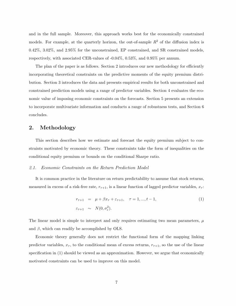
It is common practice in the literature on return predictability to assume that stock returns,

measured in excess of a risk-free rate, rτ+1, is a linear function of lagged predictor variables, xτ :

rτ+1 = µ+ βxτ + ετ+1, τ = 1, ..., t− 1, (1)

ετ+1 ∼ N(0, σ2ε).

The linear model is simple to interpret and only requires estimating two mean parameters, µ

and β, which can readily be accomplished by OLS.

Economic theory generally does not restrict the functional form of the mapping linking

predictor variables, xτ , to the conditional mean of excess returns, rτ+1, so the use of the linear

specification in (1) should be viewed as an approximation. However, we argue that economically

motivated constraints can be used to improve on this model.

7

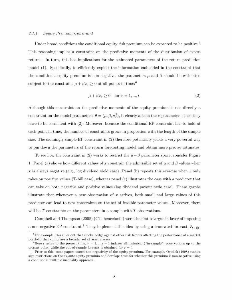
2.1.1. Equity Premium Constraint

Under broad conditions the conditional equity risk premium can be expected to be positive.5

This reasoning implies a constraint on the predictive moments of the distribution of excess

returns. In turn, this has implications for the estimated parameters of the return prediction

model (1). Specifically, to efficiently exploit the information embedded in the constraint that

the conditional equity premium is non-negative, the parameters µ and β should be estimated

subject to the constraint µ+ βxτ ≥ 0 at all points in time:6

µ+ βxτ ≥ 0 for τ = 1, ..., t. (2)

Although this constraint on the predictive moments of the equity premium is not directly a

constraint on the model parameters, θ = (µ, β, σ2ε), it clearly affects these parameters since they

have to be consistent with (2). Moreover, because the conditional EP constraint has to hold at

each point in time, the number of constraints grows in proportion with the length of the sample

size. The seemingly simple EP constraint in (2) therefore potentially yields a very powerful way

to pin down the parameters of the return forecasting model and obtain more precise estimates.

To see how the constraint in (2) works to restrict the µ−β parameter space, consider Figure

1. Panel (a) shows how different values of x constrain the admissible set of µ and β values when

x is always negative (e.g., log dividend yield case). Panel (b) repeats this exercise when x only

takes on positive values (T-bill case), whereas panel (c) illustrates the case with a predictor that

can take on both negative and positive values (log dividend payout ratio case). These graphs

illustrate that whenever a new observation of x arrives, both small and large values of this

predictor can lead to new constraints on the set of feasible parameter values. Moreover, there

will be T constraints on the parameters in a sample with T observations.

Campbell and Thompson (2008) (CT, henceforth) were the first to argue in favor of imposing

a non-negative EP constraint.7 They implement this idea by using a truncated forecast, rt+1|t,

5For example, this rules out that stocks hedge against other risk factors affecting the performance of a marketportfolio that comprises a broader set of asset classes.

6Here t refers to the present time, τ = 1, ..., t − 1 indexes all historical (“in-sample”) observations up to thepresent point, while the out-of-sample forecast is obtained for τ = t.

7Prior to this, some papers tested non-negativity of the equity premium. For example, Ostdiek (1998) studiessign restrictions on the ex-ante equity premium and develops tests for whether this premium is non-negative usinga conditional multiple inequality approach.

8

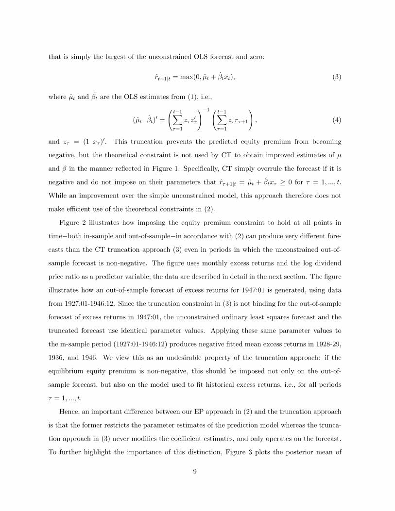
that is simply the largest of the unconstrained OLS forecast and zero:

rt+1|t = max(0, µt + βtxt), (3)

where µt and βt are the OLS estimates from (1), i.e.,

(µt βt)′ =

(t−1∑τ=1

zτz′τ

)−1( t−1∑τ=1

zτrτ+1

), (4)

and zτ = (1 xτ )′. This truncation prevents the predicted equity premium from becoming

negative, but the theoretical constraint is not used by CT to obtain improved estimates of µ

and β in the manner reflected in Figure 1. Specifically, CT simply overrule the forecast if it is

negative and do not impose on their parameters that rτ+1|t = µt + βtxτ ≥ 0 for τ = 1, ..., t.

While an improvement over the simple unconstrained model, this approach therefore does not

make efficient use of the theoretical constraints in (2).

Figure 2 illustrates how imposing the equity premium constraint to hold at all points in

time−both in-sample and out-of-sample−in accordance with (2) can produce very different fore-

casts than the CT truncation approach (3) even in periods in which the unconstrained out-of-

sample forecast is non-negative. The figure uses monthly excess returns and the log dividend

price ratio as a predictor variable; the data are described in detail in the next section. The figure

illustrates how an out-of-sample forecast of excess returns for 1947:01 is generated, using data

from 1927:01-1946:12. Since the truncation constraint in (3) is not binding for the out-of-sample

forecast of excess returns in 1947:01, the unconstrained ordinary least squares forecast and the

truncated forecast use identical parameter values. Applying these same parameter values to

the in-sample period (1927:01-1946:12) produces negative fitted mean excess returns in 1928-29,

1936, and 1946. We view this as an undesirable property of the truncation approach: if the

equilibrium equity premium is non-negative, this should be imposed not only on the out-of-

sample forecast, but also on the model used to fit historical excess returns, i.e., for all periods

τ = 1, ..., t.

Hence, an important difference between our EP approach in (2) and the truncation approach

is that the former restricts the parameter estimates of the prediction model whereas the trunca-

tion approach in (3) never modifies the coefficient estimates, and only operates on the forecast.

To further highlight the importance of this distinction, Figure 3 plots the posterior mean of

9

the coefficient estimates at each point in time from 1947-2010 for a return model that includes

the default yield spread as a predictor. The figure shows that the EP constraint leads to quite

different intercept and slope coefficient estimates than the recursive OLS estimates underlying

the truncation approach of CT. Specifically, the EP constrained estimates tend to be smoother

– though not generally closer to zero - than their OLS counterparts. This reflects the “memory”

of the learning process whereby the effect of binding constraints from the past carries over to

future periods.

The linear-normal prediction model implies that the x-variables have unbounded support.

We do not take this implication literally, and instead view this model as an approximation. We

assume that investors only impose the EP and SR constraint conditional on the data they have

seen up to a given point in time, τ = 1, ..., t. This makes the length of the initial data sample

important. Our implementation assumes a long (20-year) warm-up sample that ensures that

investors will have seen a wide range of values for xτ before making their first prediction. It

also ensures that new observations on the predictors within the historically observed range do

not tighten the constraints. Conversely, observations on the predictors outside the historical

range will trigger new learning dynamics, which we think is an attractive feature of our setup.

Moreover, we also condition on the predictor variables, treating them as exogenous rather than

as part of the data being modeled.

2.1.2. Sharpe Ratio Constraint

In this section, we explore a novel way of sharpening the forecasts of excess market returns,

namely, by placing constraints on the conditional Sharpe ratio of the market portfolio. Such

constraints might be motivated from an asset pricing perspective, as the Sharpe ratio is fre-

quently used in the calibration and evaluation of structural asset pricing models.8 In US data,

it is well-known that the Sharpe ratio is time-varying and countercyclical (Brandt (2010), Let-

tau and Ludvigson (2010)). More importantly, the empirical Sharpe ratio is quite a bit more

volatile than what the leading asset pricing models would suggest. This empirical fact has been

8See Cochrane (2001) for a textbook treatment of the Sharpe ratio’s use in evaluating asset pricing models.Lettau and Ludvigson (2010) review whether some leading asset pricing models can replicate the stylized factsregarding the Sharpe ratio in the US. Lettau and Wachter (2007) and Lettau and Wachter (2011) use the Sharperatio in the calibration of their asset pricing model.

10

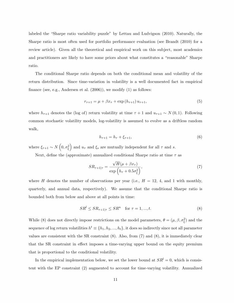
labeled the “Sharpe ratio variability puzzle” by Lettau and Ludvigson (2010). Naturally, the

Sharpe ratio is most often used for portfolio performance evaluation (see Brandt (2010) for a

review article). Given all the theoretical and empirical work on this subject, most academics

and practitioners are likely to have some priors about what constitutes a “reasonable” Sharpe

ratio.

The conditional Sharpe ratio depends on both the conditional mean and volatility of the

return distribution. Since time-variation in volatility is a well documented fact in empirical

finance (see, e.g., Andersen et al. (2006)), we modify (1) as follows:

rτ+1 = µ+ βxτ + exp (hτ+1)uτ+1, (5)

where hτ+1 denotes the (log of) return volatility at time τ + 1 and uτ+1 ∼ N (0, 1). Following

common stochastic volatility models, log-volatility is assumed to evolve as a driftless random

walk,

hτ+1 = hτ + ξτ+1, (6)

where ξτ+1 ∼ N(

0, σ2ξ

)and uτ and ξs are mutually independent for all τ and s.

Next, define the (approximate) annualized conditional Sharpe ratio at time τ as

SRτ+1|τ =

√H(µ+ βxτ )

exp(hτ + 0.5σ2ξ

) , (7)

where H denotes the number of observations per year (i.e., H = 12, 4, and 1 with monthly,

quarterly, and annual data, respectively). We assume that the conditional Sharpe ratio is

bounded both from below and above at all points in time:

SRl ≤ SRτ+1|τ ≤ SRu for τ = 1, ..., t. (8)

While (8) does not directly impose restrictions on the model parameters, θ = (µ, β, σ2ξ ) and the

sequence of log return volatilities ht ≡ {h1, h2, ..., ht}, it does so indirectly since not all parameter

values are consistent with the SR constraint (8). Also, from (7) and (8), it is immediately clear

that the SR constraint in effect imposes a time-varying upper bound on the equity premium

that is proportional to the conditional volatility.

In the empirical implementation below, we set the lower bound at SRl = 0, which is consis-

tent with the EP constraint (2) augmented to account for time-varying volatility. Annualized

11

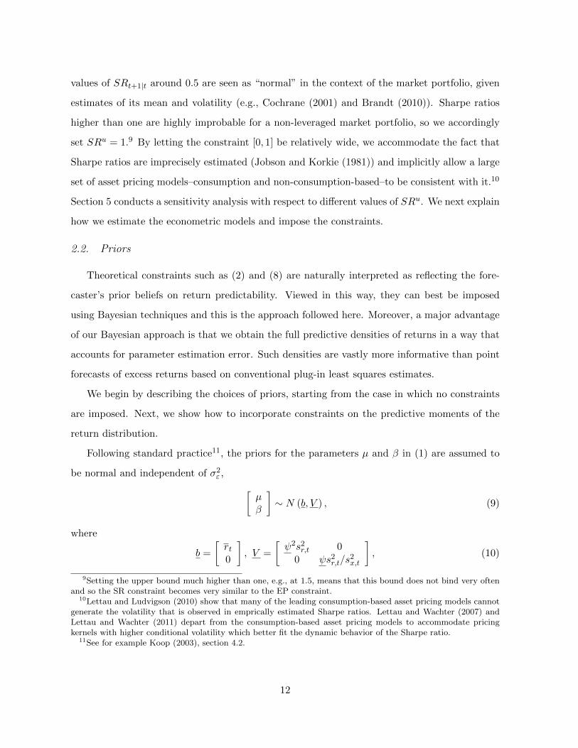
values of SRt+1|t around 0.5 are seen as “normal” in the context of the market portfolio, given

estimates of its mean and volatility (e.g., Cochrane (2001) and Brandt (2010)). Sharpe ratios

higher than one are highly improbable for a non-leveraged market portfolio, so we accordingly

set SRu = 1.9 By letting the constraint [0, 1] be relatively wide, we accommodate the fact that

Sharpe ratios are imprecisely estimated (Jobson and Korkie (1981)) and implicitly allow a large

set of asset pricing models–consumption and non-consumption-based–to be consistent with it.10

Section 5 conducts a sensitivity analysis with respect to different values of SRu. We next explain

how we estimate the econometric models and impose the constraints.

2.2. Priors

Theoretical constraints such as (2) and (8) are naturally interpreted as reflecting the fore-

caster’s prior beliefs on return predictability. Viewed in this way, they can best be imposed

using Bayesian techniques and this is the approach followed here. Moreover, a major advantage

of our Bayesian approach is that we obtain the full predictive densities of returns in a way that

accounts for parameter estimation error. Such densities are vastly more informative than point

forecasts of excess returns based on conventional plug-in least squares estimates.

We begin by describing the choices of priors, starting from the case in which no constraints

are imposed. Next, we show how to incorporate constraints on the predictive moments of the

return distribution.

Following standard practice11, the priors for the parameters µ and β in (1) are assumed to

be normal and independent of σ2ε , [µβ

]∼ N (b, V ) , (9)

where

b =

[rt0

], V =

[ψ2s2r,t 0

0 ψs2r,t/s2x,t

], (10)

9Setting the upper bound much higher than one, e.g., at 1.5, means that this bound does not bind very oftenand so the SR constraint becomes very similar to the EP constraint.

10Lettau and Ludvigson (2010) show that many of the leading consumption-based asset pricing models cannotgenerate the volatility that is observed in emprically estimated Sharpe ratios. Lettau and Wachter (2007) andLettau and Wachter (2011) depart from the consumption-based asset pricing models to accommodate pricingkernels with higher conditional volatility which better fit the dynamic behavior of the Sharpe ratio.

11See for example Koop (2003), section 4.2.

12

with data based moments

rt =1

t− 1

t−1∑τ=1

rτ+1, s2r,t =

1

t− 2

t−1∑τ=1

(rτ+1 − rt)2 ,

xt =1

t− 1

t−1∑τ=1

xτ , s2x,t =

1

t− 2

t−1∑τ=1

(xτ − xt)2 .

Here ψ is a constant that controls the tightness of the prior, with ψ → ∞ corresponding to a

diffuse prior on µ and β. Our benchmark analysis sets ψ = 2.5, but we also consider alternative

specifications with both lower and higher values of ψ. The terms s2r,t and s2r,t/s2x,t in the diagonal

of the prior variance, V , are scaling factors introduced to guarantee comparability of the priors

across different predictors and across different data frequencies.12 Our choice of the prior mean

vector b reflects the “no predictability” view that the best predictor of stock returns is the average

of past returns. We therefore center the prior intercept on the prevailing mean of historical excess

returns, while the prior slope coefficient is centered on zero. In basing the priors of some of the

hyperparameters on sample estimates−a common approach in empirical analysis, see Stock and

Watson (2006) and Efron (2010)−our analysis can be viewed as an empirical Bayes approach

rather than a more traditional Bayesian approach in which the prior distribution is fixed before

any data are observed. We show in Section 5 that the values of the hyperparameters have very

little effect on our results, thus mitigating any concerns about use of full-sample information in

setting these parameters.

Next, we specify a gamma prior for the error precision of the return innovation, σ−2ε :

σ−2ε ∼ G(s−2r,t , v0 (t− 1)

), (11)

where v0 is a prior hyperparameter that controls the degree of informativeness of this prior, with

v0 → 0 corresponding to a diffuse prior on σ−2ε .13 Our benchmark sets v0 = 0.1, which, loosely

speaking, means that the prior weight is approximately 10% of the weight put on the data.

The SR constraint (8) requires specifying a joint prior for the sequence of log return volatili-

ties, ht, and the error precision, σ−2ξ . Writing p(ht, σ−2ξ

)= p

(ht∣∣σ−2ξ ) p(σ−2ξ ), it follows from

12This aproach is used routinely in macroeconomic Bayesian VAR models. See for example Kadiyala andKarlsson (1997) and Banbura et al. (2010).

13Following Koop (2003), we adopt the Gamma distribution parametrization of Poirier (1995). Nameley, if thecontinuous random variable Y has a Gamma distribution with mean µ > 0 and degrees of freedom v > 0, wewrite Y ∼ G (µ, v) . Then, in this case, E (Y ) = µ and V ar (Y ) = 2µ2/v.

13

(6) that

p(ht∣∣σ−2ξ ) =

t−1∏τ=1

p(hτ+1|hτ , σ−2ξ

)p (h1) , (12)

with hτ+1|hτ , σ−2ξ ∼ N(hτ , σ

2ξ

). Thus, to complete the prior elicitation for p

(ht, σ−2ξ

), we

only need to specify priors for h1, the initial log volatility, and σ−2ξ . We choose these from the

normal-gamma family as follows:

h1 ∼ N (ln (sr,t) , kh) , (13)

σ−2ξ ∼ G(1/kξ, 1

). (14)

We set kξ = 0.01 and choose the remaining hyperparameters in (13) and (14) to imply uninfor-

mative priors, allowing the data to determine the degree of time variation in the return volatility.

Accordingly, we specify kh = 10, and set the degrees of freedom for σ−2ξ to 1. Section 5 discusses

robustness of our results with respect to changes in the priors.

2.3. Imposing Economic Constraints

We next describe how we impose the economic constraints on the model parameters. Starting

with the EP constraint, we modify the priors on µ and β in (9) to[µβ

]∼ N (b, V ) , µ, β ∈ At, (15)

where At is a set such that

At = {µ+ βxτ ≥ 0, τ = 1, ..., t} . (16)

Similarly, for the SR constraint, we restrict the priors on {µ, β, σ−2ξ , h1, h2, ..., ht} ∈ At, where

At is a set satisfying

At ={SRl ≤ SRτ+1|τ ≤ SRu, τ = 1, ..., t

}, (17)

and SRτ+1|τ is given in (7).

The Appendix provides details of how we estimate the parameters and compute forecasts for

the unconstrained and constrained models.

As a final point about the above analysis, we note that the boundaries of the constraints

(2) and (8) are constants (0, SRl, and SRu), motivated by economic considerations. However,

14

one might view the boundaries themselves as being parameters with associated priors. In that

case, our specification corresponds to having dogmatic priors on these specific parameters. This

generalization might be less meaningful for constraints that are readily imposed by economic

theory (such as the zero lower bound on the equity premium and Sharpe ratio) than for others

(such as the upper bound on the Sharpe ratio). From an econometric perspective, updating priors

about the boundary parameters is non-trivial. Given that the benefits of such a generalization

are not clear, while the tractability and computational costs of imposing it are substantial, we

conduct our empirical analysis by imposing constraints (2) and (8) as discussed above.

3. Empirical Results

This section presents data and empirical results using the methods for incorporating economic

constraints described in Section 2 to predict the equity premium.

3.1. Data

Our empirical analysis uses data on stock returns along with a set of seventeen predictor

variables originally analyzed in Welch and Goyal (2008) and subsequently extended up to 2010

by the same authors. Stock returns are computed from the S&P500 index and include dividends.

A short T-bill rate is subtracted from stock returns in order to capture excess returns. Data

samples vary considerably across the individual predictor variables. To be able to compare results

across the individual predictor variables, we use the longest common sample that is 1927-2010.

In addition, we use the first 20 years of data as a training sample. For example, for the monthly

data we initially estimate our regression models over the period January 1927–December 1946,

and use the estimated coefficients to forecast excess returns for January 1947. We next include

January 1947 in the estimation sample, which thus becomes January 1927–January 1947, and

use the corresponding estimates to predict excess returns for February 1947. We proceed in

this recursive fashion until the last observation in the sample, thus producing a time series of

one-step-ahead forecasts spanning the time period from January 1947 to December 2010.

The identity of the predictor variables, along with summary statistics, is provided in Table

1. Most variables fall into three broad categories, namely (i) valuation ratios capturing some

measure of ‘fundamentals’ to market value such as the dividend price ratio, the dividend yield,

15

the earnings-price ratio, the 10-year earnings-price ratio or the book-to-market ratio; (ii) mea-

sures of bond yields capturing level effects (the three-month T-bill rate and the yield on long

term government bonds), slope effects (the term spread), and default risk effects (the default

yield spread defined as the yield spread between BAA and AAA rated corporate bonds, and

the default return spread defined as the difference between the yield on long-term corporate

and government bonds); (iii) estimates of equity risk such as the long term return and stock

variance (a volatility estimate based on daily squared returns). Finally, three corporate finance

variables, namely the dividend payout ratio (the log of the dividend-earnings ratio), net equity

expansion (the ratio of 12-month net issues by NYSE-listed stocks over the year-end market

capitalization), percent equity issuing (the ratio of equity issuing activity as a fraction of total

issuing activity) and a macroeconomic variable, inflation (the rate of change in the consumer

price index), are considered.14

To make our results comparable to studies from the literature on return predictability such as

Campbell and Thompson (2008) and Welch and Goyal (2008), we focus on univariate regressions

with a single predictor variable. However, we also discuss in Section 5 how our approach can be

extended to incorporate multivariate information. Finally, since there are too many variables to

cover in detail, we focus our analysis on three predictors, namely the log dividend-price ratio, the

T-bill rate, and the default yield spread, all of which have featured prominently in the literature

on return predictability.

3.2. Coefficient Estimates and Predictive Densities

As shown in Figures 1-3, the economic constraints on the predictive moments of the return

distribution affect the parameter estimates in a way that reflects the entire sequence of data

points. This gives rise to parameter estimates that are very different from the standard, uncon-

strained ones typically applied in the literature on return predictability. To better understand

the effect of the constraints, we begin by studying the posterior distribution of the parameter

estimates.

Figure 4 plots the posterior density for the slope coefficient, β, in the equity premium equa-

tion (1) using either the log dividend-price ratio (top panel), the T-bill rate (middle), or the

14We follow Welch and Goyal (2008) and, for monthly and quarterly data, lag inflation an extra period toaccount for the delay in CPI releases.

16

default yield spread (bottom) as predictors. Posterior densities are displayed for the uncon-

strained case (solid line), the EP constraint (dark dash-dotted line), and the SR constraint

(light dark-dotted line). In each case, the unconstrained posterior density for β is considerably

wider than those of the constrained densities, suggesting that the economic constraints reduce

parameter uncertainty. Moreover, whereas the unconstrained posterior densities are symmetric,

the constrained ones are asymmetric in a direction that mostly reflects that the equity premium

has to be non-negative. For example, for the log dividend price ratio, which is always negative,

the EP constraint rules out large positive values of β, which could otherwise induce a negative

equity premium. Conversely, the constrained posterior distributions rule out large negative val-

ues of β for variables that take on positive values such as the T-bill rate and the default yield

spread. The upper bound on the Sharpe ratio also matters for the posterior distribution of β,

however, which helps explain why for positive predictors such as the T-bill rate the posterior

distribution of β under the SR constraint is shifted to the left compared with its distribution

under the EP constraint.15

To evaluate the economic significance of the changes in the parameter estimates caused by

the constraints, we next compare the ex-ante equity premium under the unconstrained and con-

strained models. To this end, Figures 5-7 show the predictive densities for the equity premium,

computed as of the end of the sample (December 2010). To illustrate how expected returns

depend on the value taken by the predictor, we show the predictive densities conditional on

xT = x as well as xT = x ± 2 × SE (x), where x and SE (x) are the full-sample average and

standard deviation of x, respectively.

First consider the results based on the log dividend-price ratio, log(D/P ) (Figure 5). This

predictor is always negative and the associated posterior estimates of β are centered on a positive

value. Comparing the plots for the three values of x illustrates how the constraints work. When

log(D/P ) is set at its sample mean (top panel), the three posterior densities have comparable

spreads, although the unconstrained model has a lower mean than the EP constrained and SR

constrained models. Reducing the log dividend-price ratio to two standard errors below its

mean (middle panel) results in a very different picture. The unconstrained posterior density

15Differences between the restricted densities do not always occur in the tail that one would expect. Thishappens because the upper constraint can be satisfied by simultaneously reducing large negative slope coefficients(as in the T-bill rate model) and shifting the density for the intercept, µ, to the right.

17

for the equity premium is now much more dispersed and shifted far further to the left, whereas

the two constrained forecasts have more probability mass to the right of zero with a tighter

support. When log(D/P ) is very low (middle panel), the lower bounds imposed by the EP

and SR constraints bind, thus preventing the probability mass from shifting to the left which

otherwise happens mechanically in a linear model (as can be seen for the unconstrained forecast).

This case is empirically relevant for the period 1990-2005 with abnormally low log dividend price

ratios. Conversely, when log(D/P ) is very high (bottom panel), the constraints are less likely

to bind, and so the three densities are more similar in shape, although once again the centers of

the distributions clearly differ.

For the T-bill rate (Figure 6), we see similar mechanisms at work, although now with the

opposite sign since the T-bill rate is always positive and the posterior estimates of β are centered

on a negative value. This means that the lower constraints now bind when the T-bill rate is set

at x + 2 × SE (x) (bottom panel), once again leading to much tighter distributions under the

EP and SR constraints than for the unconstrained case. Empirically, this occurred in the early

1980s, when the T-bill rate was particularly high. Finally, the model based on the default yield

spread (Figure 7), shows less of an asymmetry across the three conditioning scenarios regarding

the shape and spread of the conditional posterior density estimates of the equity premium.

These figures imply that the economic constraints tighten the predictive density for the

equity premium in a manner that depends asymmetrically on whether the predictor variables

take on large negative or positive values. Hence, how “informative” the bounds are, i.e., by how

much they shift and tighten the posterior density, depends on the value taken by the predictor

variable, x. We illustrate this effect in Figure 8 for the plots based on the T-bill rate.16 The top

panel plots the posterior mean of the equity premium distribution as a function of the T-bill

rate. The posterior mean declines linearly for the unconstrained model from a level near 1%

per month for the lowest values of the T-bill range to a level near zero for the highest values.17

Under the SR and EP constrained models, the posterior mean is also reduced as the T-bill rate

increases, but by far less than under the unconstrained model.

Turning to the uncertainty surrounding the predicted equity premium, the posterior vari-

16The plots for the log dividend-price ratio and default yield spread are very similar and so are omitted.17Consistent with Figure 6, the T-bill rate varies between x−2×SE (x) and x+2×SE (x) , with x and SE (x)

denoting the full-sample average and standard deviation of the T-bill rate, respectively.

18

ance of the equity premium distribution (bottom panel) is large and rises sharply under the

unconstrained model as the T-bill rate moves far away from its sample average. In contrast,

while the posterior variance of the constrained equity premium distributions does rise when the

T-bill rate takes on very small or very large values, it does so at a far slower rate. For example,

for very high values of the T-bill rate, the posterior variance of the equity premium under the

unconstrained model is close to four times higher than under the constrained models.

3.3. Forecasts of Equity Premia

Using these insights into how economic constraints affect forecasts of equity premia, we next

study the sequence of recursively generated out-of-sample equity premium forecasts. To this

end, Figure 9 presents monthly values of the mean of the predictive distribution of the equity

premium over the period 1947-2010. Economic constraints clearly make a substantial difference

during most periods. For example, the unconstrained model forecasts based on the log-dividend

price ratio (top panel) are lower and far more volatile than their constrained counterparts and

turn negative for most of the period between 1990 and 2005. Even though none of the recursive

forecasts from the unconstrained model turn negative prior to 1960, the constrained forecasts

are quite different prior to this period. As explained in Figures 2 and 3, this happens due to our

requirement that the entire sequence of model-implied fitted equity premia be non-negative. The

economic constraints lead to predicted equity premia whose differences from the unconstrained

counterparts can last very long, e.g., from 1955 through to 1975 and again from around 1985 to

the end of the sample.

Large and persistent differences in predicted mean returns are also found for the return model

based on the T-bill rate (middle panel). For this model, negative values of the unconstrained

forecasts occur most of the time between 1970 and 1985, whereas the constrained forecasts

hover around small, but positive values throughout the sample. The SR constrained forecasts

are smaller than the EP constrained forecasts for long periods of time, and both series are

notably more stable than the unconstrained equity premium forecasts.

The unconstrained equity premium forecasts based on the model that uses the default yield

spread as a predictor (bottom panel) only turn negative during the first few months of the

sample and are otherwise quite similar to the mean forecasts from the EP constrained model

19

that in turn are smaller than the SR constrained forecasts. These results are consistent with our

earlier findings that the constraints tend to bind on fewer occasions for this predictor variable.

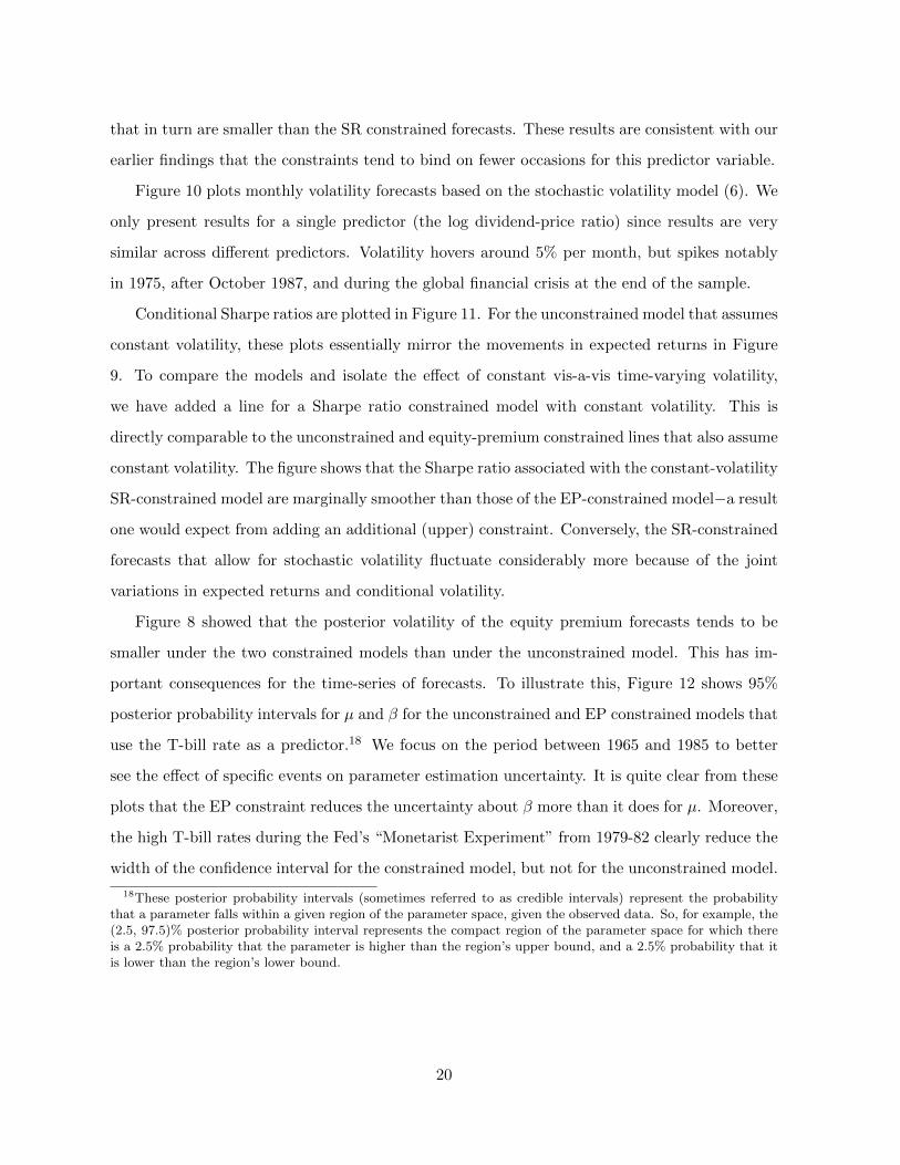
Figure 10 plots monthly volatility forecasts based on the stochastic volatility model (6). We

only present results for a single predictor (the log dividend-price ratio) since results are very

similar across different predictors. Volatility hovers around 5% per month, but spikes notably

in 1975, after October 1987, and during the global financial crisis at the end of the sample.

Conditional Sharpe ratios are plotted in Figure 11. For the unconstrained model that assumes

constant volatility, these plots essentially mirror the movements in expected returns in Figure

9. To compare the models and isolate the effect of constant vis-a-vis time-varying volatility,

we have added a line for a Sharpe ratio constrained model with constant volatility. This is

directly comparable to the unconstrained and equity-premium constrained lines that also assume

constant volatility. The figure shows that the Sharpe ratio associated with the constant-volatility

SR-constrained model are marginally smoother than those of the EP-constrained model−a result

one would expect from adding an additional (upper) constraint. Conversely, the SR-constrained

forecasts that allow for stochastic volatility fluctuate considerably more because of the joint

variations in expected returns and conditional volatility.

Figure 8 showed that the posterior volatility of the equity premium forecasts tends to be

smaller under the two constrained models than under the unconstrained model. This has im-

portant consequences for the time-series of forecasts. To illustrate this, Figure 12 shows 95%

posterior probability intervals for µ and β for the unconstrained and EP constrained models that

use the T-bill rate as a predictor.18 We focus on the period between 1965 and 1985 to better

see the effect of specific events on parameter estimation uncertainty. It is quite clear from these

plots that the EP constraint reduces the uncertainty about β more than it does for µ. Moreover,

the high T-bill rates during the Fed’s “Monetarist Experiment” from 1979-82 clearly reduce the

width of the confidence interval for the constrained model, but not for the unconstrained model.

18These posterior probability intervals (sometimes referred to as credible intervals) represent the probabilitythat a parameter falls within a given region of the parameter space, given the observed data. So, for example, the(2.5, 97.5)% posterior probability interval represents the compact region of the parameter space for which thereis a 2.5% probability that the parameter is higher than the region’s upper bound, and a 2.5% probability that itis lower than the region’s lower bound.

20

3.4. Out-of-Sample Predictive Performance

We next evaluate the predictive accuracy of the equity premium forecasts. As in Welch and

Goyal (2008) and Campbell and Thompson (2008), the predictive performance of each model is

measured relative to the prevailing mean model. The inputs to the analysis are the time series

of predictive densities of excess returns obtained as described in Section 2. To simplify the

exposition, let{rjt+1

}, j = 1, ..., J, denote draws from the predictive density of excess returns

for the prevailing mean model, conditional on data known at time t. Further, let{rjt+1,i

},

j = 1, ..., J , be draws from the predictive density of excess returns for the model based on the

ith predictor, again conditional on data known at time t. As explained in the Appendix, for

the unconstrained and EP constrained models, these draws are obtained by applying a Gibbs

sampler to

p(rt+1| Dt

)=

∫µ,β,σ−2

ε

p(rt+1|µ, β, σ−2ε ,Dt

)p(µ, β, σ−2ε

∣∣Dt) dµdβdσ−2ε , (18)

where Dt = {rτ+1, xτ}t−1τ=1 ∪xt is the information set at time t. Likewise, for the SR constrained

model, return draws are based on the predictive density

p(rt+1| Dt

)=

∫µ,β,ht+1,σ−2

ξ

p(rt+1|ht+1, µ, β, h

t, σ−2ξ ,Dt)

×p(ht+1|µ, β, ht, σ−2ξ ,Dt

)(19)

×p(µ, β, ht, σ−2ξ

∣∣∣Dt) dµdβdht+1dσ−2ξ ,

where ht+1 denotes the sequence of conditional variance states up to time t+ 1.

To compare our results with conventional performance measures used in the literature (see,

e.g., Welch and Goyal (2008), Campbell and Thompson (2008), and Rapach and Zhou (2012)),

we compute the posterior mean from the densities in (18) or (19) to obtain point forecasts.

Specifically, define time t forecast errors for the prevailing mean model and the model based on

predictor i as

et = rt −1

J

J∑j=1

rjt , t = t, ..., t, (20)

et,i = rt −1

J

J∑j=1

rjt,i, t = t, ..., t, (21)

21

where t and t denote the beginning and the end of the forecast evaluation period, respectively.

The period-t difference in the cumulative sum of squared errors (SSE) between the prevailing

mean and the ith predictor model is then equal to

∆CumSSEt =t∑

τ=t

e2τ −t∑

τ=t

e2τ,i, (22)

while the out-of-sample R2 is

R2OoS,i = 1−

∑tτ=t e

2τ,i∑t

τ=t e2τ

. (23)

Importantly, in these calculations, we only make use of historically available information

to estimate our models and generate forecasts of excess returns. For example, in (22), only

information up to period τ − 1 is used to forecast excess returns for period τ . Thus, for the first

forecast (t) we only use information up to period t − 1 to generate the forecast; for the second

forecast (t+ 1), we only use information up to period t, and so forth.

Table 2 presents the out-of-sample R2 for the unconstrained, truncated, EP and SR con-

strained forecasts estimated on monthly data. Out of the 16 unconstrained forecast models,

12 produce negative R2OoS . In contrast, the EP constrained monthly forecasts only generate

a negative R2OoS for three of the 16 variables whereas the SR constrained models generate a

negative R2OoS for six variables.

Compared with the unconstrained forecasts, the truncated approach increases the R2OoS for

12 of 16 variables, whereas the EP and SR constrained forecasts lead to a higher R2OoS for 14

out of 16 variables. This better performance is also reflected in the average R2OoS computed

across the univariate prediction models that is -0.53% for the unconstrained models, -0.22% for

the truncated forecasts, 0.19% for the EP constrained model, and 0.18% for the SR constrained

models. Notable improvements are seen for the models based on valuation ratios such as the

dividend yield or earnings-price ratio.

The results also show that the equity premium approach generally performs much better

than the truncation approach. Specifically, compared with the truncation approach, the equity

premium constraint improves the predictive accuracy for 14 out of 16 predictors and increases

the average R2OoS by 0.41% (from -0.22% to 0.19%).

Panels B and C in Table 2 show that the improvement in forecast performance resulting from

imposing the economic constraints carries over to the two subsamples 1947-1978 and 1979-2010,

22

obtained by splitting the forecast evaluation period in two halves. In the first subsample, the

average improvement in the R2OoS−values is between 0.60% and 0.70% (from -0.17% for the

unconstrained to 0.44% and 0.55% for the EP and SR constrained models, respectively). It is a

slightly better 0.70%-0.80% in the second subsample (from -0.80% for the average unconstrained

model to 0.01% and -0.10% for the EP and SR constrained models).

For the quarterly models (Table 3), the benefits from imposing economic constraints on

the equity premium forecasts get even bigger. At this frequency, we find that the EP and SR

constrained forecasts generate a higher R2OoS for 14 out of 15 predictors. Moreover, whereas the

average R2OoS is -2.33% for the unconstrained model, it is 0.47% and 1.02% for the EP and SR

constrained models, respectively. Again, notable improvements are seen for the models based on

valuation ratios such as the dividend yield or earnings-price ratio. Improvements in the average

R2OoS due to imposing economic constraints again carry over to the two subsamples and exceed

2.2% in the first subsample (1947-1978) and 3.2% in the second subsample, although the latter

reflects a clear deterioration in the performance of the unconstrained model during the period

1979-2010.

Again, it is interesting to compare the performance of the truncation approach to that of

our EP-constrained model. At the quarterly horizon we find that the EP approach delivers a

higher R2OoS−value for all but two predictors and improves the average R2

OoS−value by 1.5%

(from -1.03% to 0.47%).

Turning to the annual results, Table 4 shows that 14 of the 16 unconstrained models generate

a negative R2OoS , the average R2

OoS being -5.27%. In contrast, all of the constrained forecasts

generate a positive R2OoS , in each case higher than that of the corresponding unconstrained

model.19 Moreover, the average R2OoS computed across the 16 prediction models tends to be

quite high: 3.10% for the EP constrained models and 3.86% for the SR constrained models.

Once again, imposing the constraints lowers the probability of very poor forecast performance.

For example, the lowest R2OoS-value of any unconstrained model is -16.2% in the annual data,

versus 0.07% for the EP constrained model and 3.15% for the SR constrained models. At the

19The stochastic volatility model (6) is used to capture time-varying volatility at the monthly and quarterlyhorizons. At the annual horizon we found that there were too few observations to reliably identify the parametersof this model and ensure convergence of the parameter estimates. Instead we use a simple AR(1) specification forthe realized variance to model the variance at the annual horizon.

23

annual horizon, the EP constrained models improve the average R2OoS−value of the truncated

forecasts by 5.19% (from -2.09% to 3.10%).

Following Rapach et al. (2010), we use stars in tables 2-4 to indicate the statistical signifi-

cance of pair-wise differences in the predictive accuracy between a given forecasting model and

the benchmark model based on the Clark and West (2007) p-values.20 Economically constrained

models appear to produce significantly better return forecasts than the unconstrained forecasts

for most of the valuation ratios and many of the interest rate variables. Moreover, the results

tend to get stronger at the quarterly and annual forecast horizons.

The results in tables 2-4 indicate that the superior performance of the constrained forecasts

relative to the prevailing mean tends to strengthen as the forecast horizon grows from monthly

via quarterly to annual, whereas the opposite happens for the unconstrained forecasts. Two

effects are at play here. On the one hand, the power of the predictive signal tends to increase, the

longer the forecast horizon. On the other hand, forecasts become more uncertain at the longer

horizons as a result of the fewer data points available for estimation. For the unconstrained

models, the second effect clearly dominates and so forecast performance tends to deteriorate as

the horizon is extended. Conversely, the economic constraints provide an effective way to deal

with parameter estimation error and so the performance of the constrained models improves as

we move from the monthly to the annual horizon.

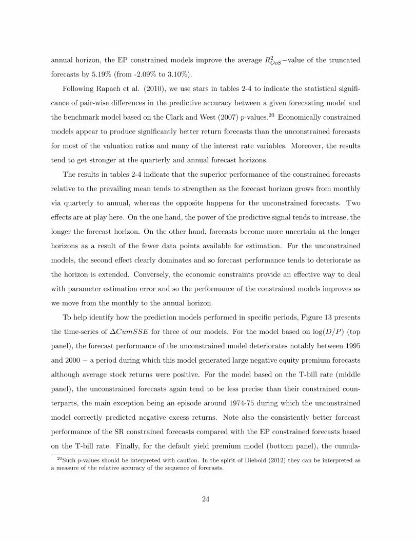
To help identify how the prediction models performed in specific periods, Figure 13 presents

the time-series of ∆CumSSE for three of our models. For the model based on log(D/P ) (top

panel), the forecast performance of the unconstrained model deteriorates notably between 1995

and 2000 − a period during which this model generated large negative equity premium forecasts

although average stock returns were positive. For the model based on the T-bill rate (middle

panel), the unconstrained forecasts again tend to be less precise than their constrained coun-

terparts, the main exception being an episode around 1974-75 during which the unconstrained

model correctly predicted negative excess returns. Note also the consistently better forecast

performance of the SR constrained forecasts compared with the EP constrained forecasts based

on the T-bill rate. Finally, for the default yield premium model (bottom panel), the cumula-

20Such p-values should be interpreted with caution. In the spirit of Diebold (2012) they can be interpreted asa measure of the relative accuracy of the sequence of forecasts.

24

tive squared errors of the unconstrained forecasts are almost uniformly worse than those of the

constrained forecasts.

In summary, economically motivated constraints on the equity premium predictions lead

to substantially better forecast performance at the monthly, quarterly, and annual horizons.

They also reduce the risk of selecting a bad forecast model which is important in situations,

such as here, characterized by considerable model uncertainty. Much of the benefit of our

approach is obtained under the (simpler) EP constraint−although the SR constraint clearly

leads to systematic improvements in forecast precision at the longer (quarterly and annual)

horizons. Both the SR and EP methods utilize the power of imposing the constraints on the

coefficient estimates learned from the data t = 1, ..., t, and so take advantage of the more efficient

learning mechanism compared with the truncation approach that does not modify the parameter

estimates in light of violations of the bounds.

4. Economic Performance and Portfolio Choice

So far we have compared the statistical performance of return forecasts generated by eco-

nomically constrained prediction models to the performance of unconstrained models. We next

evaluate the economic significance of these return forecasts by considering the optimal portfolio

choice of an investor who uses the return forecasts. An advantage of our approach is that it

accounts for parameter estimation error−a point whose importance has been emphasized by

Barberis (2000). Moreover, our approach provides the full predictive density which means that

we are not reduced to considering only mean-variance utility but can use utility functions such

as power utility with better properties.

4.1. Framework

Consider the optimal asset allocations of a representative investor with utility function U .

At time t, the investor solves the optimal asset allocation problem

ω∗t = arg maxωt

E[U (ωt, rt+1)| Dt

], (24)

25

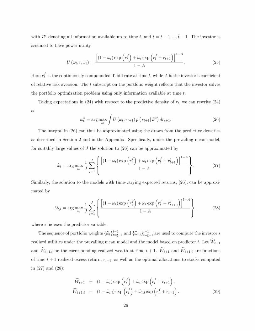
with Dt denoting all information available up to time t, and t = t− 1, ..., t− 1. The investor is

assumed to have power utility

U (ωt, rt+1) =

[(1− ωt) exp

(rft

)+ ωt exp

(rft + rt+1

)]1−A1−A

. (25)

Here rft is the continuously compounded T-bill rate at time t, while A is the investor’s coefficient

of relative risk aversion. The t subscript on the portfolio weight reflects that the investor solves

the portfolio optimization problem using only information available at time t.

Taking expectations in (24) with respect to the predictive density of rt, we can rewrite (24)

as

ω∗t = arg maxωt

∫U (ωt, rt+1) p

(rt+1| Dt

)drt+1. (26)

The integral in (26) can thus be approximated using the draws from the predictive densities

as described in Section 2 and in the Appendix. Specifically, under the prevailing mean model,

for suitably large values of J the solution to (26) can be approximated by

ωt = arg maxωt

1

J

J∑j=1

[(1− ωt) exp

(rft

)+ ωt exp

(rft + rjt+1

)]1−A1−A

. (27)

Similarly, the solution to the models with time-varying expected returns, (26), can be approxi-

mated by

ωt,i = arg maxωt

1

J

J∑j=1

[(1− ωt) exp

(rft

)+ ωt exp

(rft + rjt+1,i

)]1−A1−A

, (28)

where i indexes the predictor variable.

The sequence of portfolio weights {ωt}t−1t=t−1 and {ωt,i}t−1t=t−1 are used to compute the investor’s

realized utilities under the prevailing mean model and the model based on predictor i. Let Wt+1

and Wt+1,i be the corresponding realized wealth at time t + 1. Wt+1 and Wt+1,i are functions

of time t+ 1 realized excess return, rt+1, as well as the optimal allocations to stocks computed

in (27) and (28):

Wt+1 = (1− ωt) exp(rft

)+ ωt exp

(rft + rt+1

),

Wt+1,i = (1− ωt,i) exp(rft

)+ ωt,i exp

(rft + rt+1

). (29)

26

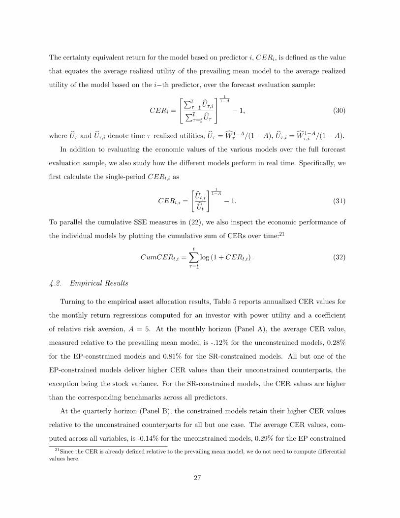
The certainty equivalent return for the model based on predictor i, CERi, is defined as the value

that equates the average realized utility of the prevailing mean model to the average realized

utility of the model based on the i−th predictor, over the forecast evaluation sample:

CERi =

∑tτ=t Uτ,i∑tτ=t Uτ

11−A

− 1, (30)

where Uτ and Uτ,i denote time τ realized utilities, Uτ = W 1−Aτ /(1−A), Uτ,i = W 1−A

τ,i /(1−A).

In addition to evaluating the economic values of the various models over the full forecast

evaluation sample, we also study how the different models perform in real time. Specifically, we

first calculate the single-period CERt,i as

CERt,i =

[Ut,i

Ut

] 11−A

− 1. (31)

To parallel the cumulative SSE measures in (22), we also inspect the economic performance of

the individual models by plotting the cumulative sum of CERs over time:21

CumCERt,i =t∑

τ=t

log (1 + CERt,i) . (32)

4.2. Empirical Results

Turning to the empirical asset allocation results, Table 5 reports annualized CER values for

the monthly return regressions computed for an investor with power utility and a coefficient

of relative risk aversion, A = 5. At the monthly horizon (Panel A), the average CER value,

measured relative to the prevailing mean model, is -.12% for the unconstrained models, 0.28%

for the EP-constrained models and 0.81% for the SR-constrained models. All but one of the

EP-constrained models deliver higher CER values than their unconstrained counterparts, the

exception being the stock variance. For the SR-constrained models, the CER values are higher

than the corresponding benchmarks across all predictors.

At the quarterly horizon (Panel B), the constrained models retain their higher CER values

relative to the unconstrained counterparts for all but one case. The average CER values, com-

puted across all variables, is -0.14% for the unconstrained models, 0.29% for the EP constrained

21Since the CER is already defined relative to the prevailing mean model, we do not need to compute differentialvalues here.

27

models and 0.32% for the SR constrained models. Finally, at the annual horizon (Panel C),

the average CER value is -0.24% for the unconstrained models, 0.33% for the EP constrained

models and 0.67% for the SR constrained models and the constrained models produce higher

CER values than the unconstrained counterparts for every single predictor.

Comparing the results under the truncation approach of Campbell and Thompson (2008) to

those under the EP constraint, Table 5 shows that, with one exception (stock variance, monthly

horizon), the EP approach generates higher CER values for all predictors at all horizons. The

average improvement in CER values is 0.35% (from -0.07% to 0.28%), 0.37% (from -0.08% to

0.29%), and 0.50% (from -0.17% to 0.33%) at the monthly, quarterly, and annual horizons,

respectively. Given the better performance under the EP constraint than under the truncation

approach, we do not report further results from the latter.

In Table 6, we show that the observed improvements in economic utility carry over to our

two subsamples. There again, the constrained models do better than the unconstrained ones

for the vast majority of cases. Interestingly, there is no evidence that the economic benefits

from using economically constrained forecasts deteriorates over time. For example, over the

subsample 1979-2010 the mean CER value for the annual model is -0.62% for the unconstrained

model and 0.08% and 0.76% for the EP and SR constrained models − a bigger differential than

in the earlier subsample 1947-78.

Using the log dividend-price ratio as a predictor, Figure 14 plots the sequence of stock port-

folio weights along with the cumulative (continuously compounded) CER estimates computed

according to Equation (32). The portfolio weights vary considerably over time under the uncon-

strained and SR-constrained model that allows for stochastic volatility, but are much smoother

under the EP constraint and the constant-volatility SR-constrained model. Moreover, the cu-

mulative CER values of the constrained models consistently lie above the CER estimates of the

unconstrained model. At the end of the sample, the cumulative CER value of the unconstrained

model is around -30%, whereas it exceeds 20% and 80% for the EP and SR (stochastic volatility)

constrained models, respectively. These numbers capture the cumulative risk-adjusted economic

value of the economically constrained forecasts relative to the prevailing mean forecasts.

We conclude that there are economically large benefits from imposing economic constraints

on the equity premium prediction models. The benefits appear to be present at monthly, quar-

28

terly, and annual horizons and are largest for the SR constraint that allows for time-varying

volatility. Moreover, the benefits do not appear to be deteriorating over time.

5. Extensions and Robustness Analysis

This section extends our analysis to incorporate multivariate information. Moreover, we

present a range of sensitivity analyses that shed light on the robustness of our findings.

5.1. Multivariate Results

So far, we have followed much of the finance literature on return predictability and focused

on univariate prediction models. We next extend the analysis to a multivariate setting. With

N predictor variables available, there are N different predictive densities. Using i to index

the predictors as we have done above, we denote these predictive densities by p(rt+1| Dt,Mi

),

i = 1, ..., N , where Mi refers to model i. Instead of conditioning only on a single predictor,

investors may want to take advantage of the information contained in all of the N predictors.

We consider two different ways to combine the information contained in N different predictors.

The first approach relies on forecast combination methods. Specifically, we construct a

combined predictive density as an equal-weighted average of the N predictive densities

p(rt+1| Dt

)=

N∑i=1

wi,t × p(rt+1| Dt,Mi

), (33)

where wi,t = 1/N for all i and t = t−1, ..., t−1. We compute the equal weighted predictive density

in (33) across all predictor variables applying this approach separately to the unconstrained, EP

and SR constrained models. For point forecasts, this approach was previously adopted by

Rapach et al. (2010).

Our second approach relies on diffusion indexes. As shown by Stock and Watson (2006),

diffusion indexes provide a convenient framework for extracting the key common drivers from

a large number of potential predictors. Ludvigson and Ng (2007) and Neely et al. (2012) show

that diffusion indexes can be used to improve equity premium forecasting.

The diffusion index approach assumes a common factor structure for the N potential pre-

dictors,

xiτ = λ′ifτ + ei,τ , τ = 1, ..., t− 1 (34)

29

where i indexes the predictor, λ is a (q × 1) vector of factor loadings (q << N), fτ is a (q × 1)

vector of latent factors containing the common components extracted from the N predictors,

and ei,τ is a zero-mean disturbance term. Following Rapach et al. (2010), we restrict our analysis

to considering a single factor; the results do not appear to improve if we include two or more

factors in the model.

We estimate the common factors using principal components, and use them as predictors for

stock returns in the following equation:

rτ+1 = µDI + βDIfτ + ετ+1, τ = 1, ..., t− 1, (35)

where βDI is a (q × 1) vector of slope coefficients and ετ+1 ∼ N(

0, σ2ε,DI

). As for the univariate

models in Section 2, we specify an independent normal-gamma prior for the parameters in (35),

and use a Gibbs sampler for estimation. Next, draws from the corresponding predictive density

are obtained as

p(rt+1| Dt

)=

∫µDI ,βDI ,σ

−2ε,DI

p(rt+1|µDI , βDI , σ−2ε,DI ,D

t)

(36)

×p(µDI , βDI , σ

−2ε,DI

∣∣∣Dt) dµDIdβDIdσ−2ε,DIwhere p

(µDI , βDI , σ

−2ε,DI

∣∣∣Dt) is the joint posterior density of all parameters in (35). We estimate

the diffusion index model in (35) and derive the predictive density in (36) for the unconstrained,

EP constrained, and SR constrained models.

5.1.1. Empirical Findings

Table 7 presents empirical results for the equal-weighted combination as well as for the

diffusion index. First consider the statistical measures of forecast performance. In all cases these

improve when compared to the average forecast performance computed across the individual

models. At all three horizons, the equal weighted combination yields the largest improvement

in R2OoS−performance for the unconstrained models. For example, at the monthly horizon the

equal-weighted combination of unconstrained forecasts generates a R2OoS of 0.62% versus -0.53%

as the average value of the individual models. We also see improvements for the constrained

models, but these tend to be smaller. Which equal-weighted combination is best depends on the

frequency: At the monthly horizon, combining unconstrained forecasts seem to work best; at

30

the quarterly horizon, combining the SR constrained forecasts produces the best performance,

while at the annual horizon the three approaches perform comparably.

The performance improves even more in the case of the diffusion index that works particu-

larly well under the economic constraints. In fact, the EP-constrained forecasts deliver higher

R2OoS−values than the equal-weighted unconstrained forecasts at all three horizons, and across

both subsamples. The SR-constrained forecasts based on the diffusion index also perform very

well.

Turning to the economic performance measures, again, these generally lead to higher CER

values when compared against the average values produced by the individual univariate models.

While the benefit from using equal-weighted forecasts remains largest for the unconstrained

forecasts, the resulting CER values are always smaller than those produced by the corresponding

equal-weighted constrained forecasts with differences ranging from 0.13% to 0.31% for the EP-

constrained forecasts, and from 0.39% to 0.72% for the SR-constrained forecasts. Moreover,

the best results from using the diffusion index is obtained for the constrained forecasts with

differences ranging from 0.51% to 0.71% for the EP-constrained forecasts and from 0.99% to

1.27% for the SR-constrained forecasts. In fact, the diffusion index approach works better than

the equal-weighted combination for the EP-constrained and the SR-constrained cases at all

horizons.

5.2. Performance in Recessions and Expansions

Table 8 shows results separately for recession and expansion periods as defined by the NBER

indicator and applied to the monthly and quarterly data. This type of analysis has been pro-

posed by authors such as Rapach et al. (2010) and Henkel et al. (2011). Consistent with the

findings in these studies, the unconstrained return prediction models perform better versus the

prevailing mean during recessions than during expansions. Interestingly, the converse holds

for the constrained monthly forecasts that far outperform the unconstrained forecasts during

expansions, but perform worse during recessions.

While seemingly surprising, this finding can be explained by the fact that the state variable

being sorted on (recessions) is correlated with returns. Returns tend to be negative during

recessions and positive during expansions and so models that impose non-negative predictions

31

will almost by construction do relatively better during expansions and worse during recessions.

Despite this effect, at the quarterly horizon the EP constrained forecasts do almost as well

as the unconstrained forecasts during recessions (and much better during expansions), while the

SR constrained forecasts do substantially better than the unconstrained forecasts both during

expansions and recessions.

5.3. Upper bound on Sharpe Ratio

In practice it can be difficult to determine the upper bound on “reasonable” Sharpe ratios.

Ross (1976) introduces asset pricing constraints by assuming that portfolios cannot have Sharpe

ratios greater than twice the Sharpe ratio of the market portfolio, which would be roughly in

line (though a bit below) with the upper bound SRu = 1 that we focus on here. Cochrane and

Saa-Requejo (2000) are less specific but point out that there is a “long tradition in finance that

regards high Sharpe ratios as ‘good deals‘ that are unlikely to survive, since investors would

quickly grab them up.”

One way to approach this issue is to view the upper bound as another parameter about

which there is uncertainty and then conduct a sensitivity analysis. To this end, Table 9 shows

results for the three predictors of particular focus (the dividend-price ratio, the T-bill rate, and

the default yield spread) for a wide range of values for the upper bound on the Sharpe ratio

{0.5, 0.75, 1, 1.25, 1.5}. The table shows that the R2OoS-value is even higher than in the baseline

scenario with SRu = 1 when the upper bound is set to 0.75, rather than at one, although for

two of the predictors (the dividend-price ratio and the T-bill rate), a larger value of the upper

bound (SRu = 1.25) gives the best results. At the quarterly and annual horizons (not shown),

slight improvements are observed (relative to the benchmark SRu = 1) by either increasing or

decreasing SRu by 0.25, but the conclusions about the performance of the return forecasts under

the SR constraint again appear robust.22

22Another perspective on this issue is that, given one’s beliefs on what may constitute a reasonable upper boundon the Sharpe ratio, we can use our proposed methodology to impose the resulting constraint on the predictiveregression.

32

5.4. Sensitivity to Risk Aversion

Our main analysis of the economic value of equity premium forecasts in Section 4 assumed

a coefficient of relative risk aversion of A = 5. To explore the sensitivity of our results to this

value, we also consider lower (A = 2) and higher (A = 10) values of this parameter. Results are

shown in Table 10.

First consider the case with A = 2, i.e., lower risk aversion compared with the baseline case,

A = 5. At the monthly horizon, the average CER performance of the unconstrained performance

models is reduced from -0.12% to -0.27%, while conversely the average CER value of the EP

constrained models increases from 0.28% to 0.68% and the SR constrained models’ average

performance is essentially unchanged at 0.79%. At the quarterly horizon, the mean CER value

of the unconstrained forecasts remains unchanged, while the mean CER values under the EP

and SR constraints increase from around 0.3% to 0.8% and 1.0%, respectively. Similarly, the

constrained models’ mean CER values increase to 0.83% and 1.03%, respectively (previously

0.33% and 0.67%) at the annual horizon, whereas the unconstrained model’s mean CER value,

at -0.07%, remains negative (previously -0.24%). Lowering the coefficient of risk aversion from

A = 5 to A = 2 thus has the effect of boosting the economic performance of the constrained

models whose mean CER value exceeds that of the unconstrained model by more than 0.90%

(EP constraint) and 1.06% (SR constraint).

Conversely, increasing the risk aversion from A = 5 to A = 10 reduces the spread in the

performance of the different models, as an investor with such a high level of risk aversion re-

frains from taking large positions in equity even in the presence of strong evidence of return

predictability. At this higher level of risk aversion, the constrained models continue to out-

perform the unconstrained ones, although the difference in average CER values is reduced to

between 0.2% and 0.35% for the EP constrained models and to between 0.3% and 0.5% for the

SR constrained models.

5.5. Sensitivity to Priors

We also test the robustness of our results to alternative prior assumptions, and perform

a sensitivity analysis in which we experiment with different values for some of the key prior

hyperparameters. Given the similarities in the results obtained under the models based on the

33

EP and SR constraints, as well as the more computationally demanding estimation algorithm

required by models imposing the SR constraint, we focus our attention on the effectiveness

of the equity premium constraint as the priors change, and explore the effect of altering the

hyperparameter ψ and v0 in (10) and (11). As discussed in section 2.2, the hyperparameter

ψ plays the role of a scaling factor controlling the tightness of the priors for µ and β, and our

benchmark models set ψ = 2.5. As sensitivities, we experiment with ψ = 1.25 and ψ = 5, which

imply more concentrated prior distributions (in the case of ψ = 1.25) or more dispersed prior

distributions (in the case of ψ = 5) for µ and β. Similarly, the prior parameter v0 controls the

tightness of the prior for σ−2ε , and our benchmark models set v0 = 0.1, which corresponds to a

hypothetical prior sample size as large as 10% of the actual sample.23 In a sensitivity analysis,

we experiment with v0 = 0.5 and v0 = 0.05, which imply, respectively, an hypothetical prior

sample as large as 50% of the underlying estimation sample (in the case of v0 = 0.5), or as large

as 5% of the underlying estimation sample (in the case of v0 = 0.05). Representing an even

greater detour from the baseline priors, we also consider values of ψ = 0.5, v0 = 1, corresponding

to very precise priors, and ψ = 10, v0 = 0.01 corresponding to very diffuse priors.

Table 11 and Table 12 summarize the (relative) statistical and economic performances of

both unconstrained and equity premium constrained models under these four alternative prior

choices, over the period 1947-2010. A comparison with tables 2, 3, 4, and 5 reveal that the key

results derived under the benchmark priors remain largely unaffected when the priors change,

with perhaps the only noticeable difference being related to the Clark and West (2007) p-values

in table 11 for the more dispersed prior choices, which is a direct consequence of the slightly

wider predictive densities resulting from this prior. For the unconstrained model, the best

results are generally associated with tighter priors that tend to reduce the effect of parameter

estimation errors. Conversely, for the EP-constrained forecasts, we obtain slightly better results

for the more diffuse priors, although variations in results across different priors are minor. Thus,

our findings are robust to choosing ψ and v0 to take on very different values from those in the

baseline analysis.

23Under conjugate priors, the information contained in the priors can be viewed as “fictitious sample informa-tion” in that it is combined with the sample in exactly the same way that additional sample information wouldbe combined (see Koop (2003)).

34

5.6. Other predictor variables

So far we focused our empirical analysis exclusively on the predictor variables considered by

Welch and Goyal (2008). One additional predictor variable that has recently garnered consid-

erable interest is the single factor extracted from the cross-section of book-to-market ratios by

Kelly and Pruitt (2012). For comparison, we compute the out-of-sample R2 obtained from this

predictor for the same sample period as that used here, 1947-2012.24 For the unconstrained, EP

and SR constrained models, we obtain R2−values of 0.16, -0.16, and 0.01, respectively. This

suggests, first, that the economic constraints do not improve the forecasts from a linear regres-

sion model based on this particular predictor variable. Second, however, it is interesting to note

that many of our models produce higher out-of-sample R2-values than those obtained for this

new predictor variable.

6. Conclusion

We develop a new methodology for imposing constraints that rule out negative equity premia

and bound the conditional Sharpe ratio from above and below. Our approach efficiently exploits

the information in such constraints in a way that incorporates the entire sequence of data points,

while accounting for parameter uncertainty.

When evaluated empirically, we find that a key effect of the economic constraints is to

reduce the impact of “large” values of the predictor variables on the expected equity premium.

Conventional linear models tend to generate noisy forecasts following large variations in the

predictor variables. In contrast, economic constraints effectively shrink the predicted equity

premium and reduce the effect of outliers since they are more likely to bind for “large” values

of the predictor variables. This gives rise to dynamic learning effects that can shift the entire

predictive distribution for the equity premium even in situations in which no such change is

observed under a conventional unconstrained model.

Imposing economic constraints on the equity premium forecast improves the predictive ac-

curacy for nearly all of the prediction models we consider. Moreover, the benefits from the

economic constraints seem to improve, the longer the forecast horizon. In turn, when used to

24We are gratefull to Seth Pruitt for making the data available to us.

35

select portfolio weights, the constrained forecasts are found to yield higher certainty equivalent

returns than their unconstrained counterparts.

References

Andersen, T. G., Bollerslev, T., Christoffersen, P. F., Diebold, F. X., 2006. Volatility and

correlation forecasting. Elsevier, vol. 1 of Handbook of Economic Forecasting , pp. 777 – 878.

Ang, A., Piazzesi, M., 2003. A no-arbitrage vector autoregression of term structure dynamics

with macroeconomic and latent variables. Journal of Monetary Economics 50, 745 – 787.

At-Sahalia, Y., Brandt, M. W., 2001. Variable selection for portfolio choice. The Journal of

Finance 56, pp. 1297–1351.

Avramov, D., Wermers, R., 2006. Investing in mutual funds when returns are predictable. Jour-

nal of Financial Economics 81, 339 – 377.

Banbura, M., Giannone, D., Reichlin, L., 2010. Large bayesian vector auto regressions. Journal

of Applied Econometrics 25, 71–92.

Barberis, N., 2000. Investing for the long run when returns are predictable. The Journal of

Finance 55, 225 – 264.

Bossaerts, P., Hillion, P., 1999. Implementing statistical criteria to select return forecasting

models: what do we learn? Review of Financial Studies 12, 405–428.

Boudoukh, J., Richardson, M., Smith, T., 1993. Is the ex ante risk premium always positive?:

A new approach to testing conditional asset pricing models. Journal of Financial Economics

34, 387 – 408.

Brandt, M. W., 2010. Portfolio choice problems. Handbook of Financial Econometrics 1, 269 –

336.

Brennan, M. J., Schwartz, E. S., Lagnado, R., 1997. Strategic asset allocation. Journal of Eco-

nomic Dynamics and Control 21, 1377 – 1403.

36

Campbell, J., Shiller, R., 1988. The dividend-price ratio and expectations of future dividends

and discount factors. Review of Financial Studies 1, 195–228.

Campbell, J. Y., 1987. Stock returns and the term structure. Journal of Financial Economics

18, 373 – 399.

Campbell, J. Y., Thompson, S. B., 2008. Predicting excess stock returns out of sample: Can

anything beat the historical average? Review of Financial Studies 21, 1509–1531.

Campbell, J. Y., Viceira, L. M., 1999. Consumption and portfolio decisions when expected

returns are time varying. The Quarterly Journal of Economics 114, 433–495.

Carter, C. K., Kohn, R., 1994. On gibbs sampling for state space models. Biometrika 81, pp.

541–553.

Clark, T. E., West, K. D., 2007. Approximately normal tests for equal predictive accuracy in

nested models. Journal of Econometrics 138, 291 – 311.

Cochrane, J. H., 2001. Asset pricing. Princeton University Press.

Diebold, F. X., 2012. Comparing predictive accuracy, twenty years later: A personal perspective

on the use and abuse of diebold-mariano tests, working paper, University of Pennsylvania.

Durbin, J., Koopman, S. J., 2002. A simple and efficient simulation smoother for state space

time series analysis. Biometrika 89, pp. 603–615.

Efron, B., 2010. Large-Scale Inference: Empirical Bayes Methods for Estimation, Testing, and

Prediction. Cambridge University Press.

Fama, E. F., French, K. R., 1988. Dividend yields and expected stock returns. Journal of Fi-

nancial Economics 22, 3 – 25.

Fama, E. F., French, K. R., 1989. Business conditions and expected returns on stocks and bonds.

Journal of Financial Economics 25, 23 – 49.

Ferson, W. E., Harvey, C. R., 1991. The variation of economic risk premiums. Journal of Political

Economy 99, pp. 385–415.

37

Ferson, W. E., Schadt, R. W., 1996. Measuring fund strategy and performance in changing

economic conditions. The Journal of Finance 51, pp. 425–461.

Goyal, A., Welch, I., 2003. Predicting the equity premium with dividend ratios. Management

Science 49, pp. 639–654.

Henkel, S. J., Martin, J. S., Nardari, F., 2011. Time-varying short-horizon predictability. Journal

of Financial Economics 99, 560 – 580.

Jobson, J. D., Korkie, B. M., 1981. Performance hypothesis testing with the sharpe and treynor

measures. The Journal of Finance 36, pp. 889–908.

Kadiyala, K. R., Karlsson, S., 1997. Numerical methods for estimation and inference in bayesian

var-models. Journal of Applied Econometrics 12, 99–132.

Kandel, S., Stambaugh, R. F., 1996. On the predictability of stock returns: An asset-allocation

perspective. The Journal of Finance 51, pp. 385–424.

Keim, D. B., Stambaugh, R. F., 1986. Predicting returns in the stock and bond markets. Journal

of Financial Economics 17, 357 – 390.

Kelly, B. T., Pruitt, S., 2012. Market expectations in the cross section of present values. Journal

of Finance (forthcoming) .

Kim, S., Shephard, N., Chib, S., 1998. Stochastic volatility: Likelihood inference and comparison

with arch models. The Review of Economic Studies 65, 361–393.

Koop, G., 2003. Bayesian Econometrics. John Wiley & Sons, Ltd.

Lamont, O., 1998. Earnings and expected returns. The Journal of Finance 53, pp. 1563–1587.

Lettau, M., Ludvigson, S., 2001. Consumption, aggregate wealth, and expected stock returns.

The Journal of Finance 56, 815–849.

Lettau, M., Ludvigson, S. C., 2010. Measuring and modeling variation in the risk-return trade-

off. Elsevier, vol. 1 of Handbook of Financial Econometrics, pp. 617 – 690.

38

Lettau, M., Van Nieuwerburgh, S., 2008. Reconciling the return predictability evidence. Review

of Financial Studies 21, 1607–1652.

Lettau, M., Wachter, J. A., 2007. Why is long-horizon equity less risky? a duration-based

explanation of the value premium. The Journal of Finance 62, 55–92.

Lettau, M., Wachter, J. A., 2011. The term structures of equity and interest rates. Journal of

Financial Economics 101, 90 – 113.

Ludvigson, S. C., Ng, S., 2007. The empirical risk-return relation: A factor analysis approach.

Journal of Financial Economics 83, 171 – 222.

MacKinlay, A., 1995. Multifactor models do not explain deviations from the capm. Journal of

Financial Economics 38, 3 – 28.

MacKinlay, A. C., Pastor, L., 2000. Asset pricing models: Implications for expected returns and

portfolio selection. The Review of Financial Studies 13, pp. 883–916.

Neely, C., Rapach, D. E., Tu, J., Zhou, G., 2012. Forecasting the equity risk premium: The role

of technical indicators, federal Reserve Bank of St. Louis working paper.

Ostdiek, B., 1998. The world ex ante risk premium: an empirical investigation. Journal of

International Money and Finance 17, 967 – 999.

Pastor, L., Stambaugh, R. F., 2009. Predictive systems: Living with imperfect predictors. The

Journal of Finance 64, 1583–1628.

Pastor, L., Stambaugh, R. F., 2012. Are stocks really less volatile in the long run? The Journal

of Finance 67, 431–478.

Paye, B. S., Timmermann, A., 2006. Instability of return prediction models. Journal of Empirical

Finance 13, 274 – 315.

Pesaran, M. H., Timmermann, A., 1995. Predictability of stock returns: Robustness and eco-

nomic significance. The Journal of Finance 50, 1201–1228.

Poirier, D. J., 1995. Intermediate Statistics and Econometrics: A Comparative Approach. MIT

Press.

39

Polk, C., Thompson, S., Vuolteenaho, T., 2006. Cross-sectional forecasts of the equity premium.

Journal of Financial Economics 81, 101 – 141.

Pontiff, J., Schall, L. D., 1998. Book-to-market ratios as predictors of market returns. Journal

of Financial Economics 49, 141 – 160.

Rapach, D. E., Strauss, J. K., Zhou, G., 2010. Out-of-sample equity premium prediction: Com-

bination forecasts and links to the real economy. Review of Financial Studies 23, 821–862.

Rapach, D. E., Zhou, G., 2012. Forecasting stock returns, working paper - In preparation for

the Handbook of Economic Forecasting, volume 2.

Ross, S. A., 1976. The arbitrage theory of capital asset pricing. Journal of Economic Theory 13,

341 – 360.

Ross, S. A., 2005. Neoclassical finance. Princeton University Press.

Shanken, J., Tamayo, A., 2012. Payout yield, risk, and mispricing: A bayesian analysis. Journal

of Financial Economics 105, 131 – 152.

Stock, J. H., Watson, M. W., 2006. Forecasting with many predictors. Elsevier, vol. 1 of Handbook

of Economic Forecasting , pp. 515 – 554.

Wachter, J. A., Warusawitharana, M., 2009. Predictable returns and asset allocation: Should a

skeptical investor time the market? Journal of Econometrics 148, 162 – 178.

Welch, I., Goyal, A., 2008. A comprehensive look at the empirical performance of equity premium

prediction. Review of Financial Studies 21, 1455–1508.

Xia, Y., 2001. Learning about predictability: The effects of parameter uncertainty on dynamic

asset allocation. The Journal of Finance 56, 205–246.

Zhou, G., 2010. How much stock return predictability can we expect from an asset pricing

model? Economics Letters 108, 184 – 186.

40

A. Appendix

This appendix explains how we obtain parameter estimates for the models described in

Section 2, and how we use these to generate predictive densities for excess returns. We begin

by discussing the unconstrained model in (1), and next turn to the models that incorporate the

constraints in (2) and (8).

A.1. No constraints

In the unconstrained case, the goal is to obtain draws from the joint posterior distribution

p(µ, β, σ−2ε

∣∣Dt) with Dt denoting all information available up to time t. Combining the priors

in (9)-(11) with the likelihood function yields the following conditional posteriors:[µβ

]∣∣∣∣σ−2ε ,Dt ∼ N(b, V

), (A-1)

and

σ−2ε∣∣µ, β,Dt ∼ G (s−2, v) , (A-2)

where

V =

[V −1 + σ−2ε

t−1∑τ=1

zτz′τ

]−1,

b = V

[V −1b+ σ−2ε

t−1∑τ=1

zτrτ+1

], (A-3)

v = v0 + (t− 1) ,

zτ = (1 xτ )′ and

s2 =

∑t−1τ=1 (rτ+1 − µ− βxτ )2 +

(s2r,t × v0 (t− 1)

)v

. (A-4)

A Gibbs sampler algorithm can be used to iterate back and forth between (A-1) and (A-2),

yielding a series of draws for the parameter vector(µ, β, σ−2ε

). Draws from the predictive

density p(rt+1| Dt

)can then be obtained by noting that

p(rt+1| Dt

)=

∫µ,β,σ−2

ε

p(rt+1|µ, β, σ−2ε ,Dt

)p(µ, β, σ−2ε

∣∣Dt) dµdβdσ−2ε . (A-5)

41

A.2. Equity premium constraints

The approach used for the unconstrained model also works when EP constraints are imposed

subject to simply introducing an accept-reject step in (A-1):[µβ

]∣∣∣∣σ−2ε ,Dt ∼ N(b, V

)× µ, β ∈ At,

σ−2ε∣∣µ, β,Dt ∼ G

(s−2, v

), (A-6)

with At defined in Equation (16), and, once again, using Equation (A-5) to draw from the

predictive density p(rt+1| Dt

).

A.3. Conditional Sharpe Ratio Constraints

To obtain draws from the joint posterior distribution p(µ, β, ht, σ−2ξ

∣∣∣Dt) under the SR

constraints, we use the Gibbs sampler to draw recursively from the following three conditional

distributions:

1. p(ht∣∣µ, β, σ−2ξ ,Dt

).

2. p(µ, β|ht, σ−2ξ ,Dt

).

3. p(σ−2ξ

∣∣∣µ, β, ht,Dt) .We simulate from each of these blocks as follows. Starting with p

(ht∣∣µ, β, σ−2ξ ,Dt

), we

employ the algorithm of Kim et al. (1998). Define r∗τ+1 = rτ+1 − µ− βxτ and note that r∗τ+1 is

observable conditional on µ, β. Next, rewrite (5) as

r∗τ+1 = exp (hτ+1)uτ+1. (A-7)

Squaring and taking logs on both sides of (A-7) yields a new state space system that replaces

(5)-(6) with

r∗∗τ+1 = 2hτ+1 + u∗∗τ+1, (A-8)

hτ+1 = hτ + ξτ+1, (A-9)

where r∗∗τ+1 = ln(r2τ+1

), and u∗∗τ+1 = ln

(u2τ+1

), with u∗∗τ independent of ξs for all τ and s. Since

u∗∗t+1 ∼ ln(χ21

), we cannot resort to standard Kalman recursions and simulation algorithms

42

such as those in Carter and Kohn (1994) or Durbin and Koopman (2002). To obviate this

problem, Kim et al. (1998) employ a data augmentation approach and introduce a new state

variable sτ+1, τ = 1, .., t−1, turning their focus on drawing from p(ht∣∣µ, β, σ−2ξ , st,Dt

)instead

of p(ht∣∣µ, β, σ−2ξ ,Dt

).25 The introduction of the state variable sτ+1 allows us to rewrite the

linear non-Gaussian state space representation in (A-8)-(A-9) as a linear Gaussian state space

model, making use of the following approximation,

u∗∗τ+1 ≈7∑j=1

qjfN(mj − 1.2704, v2j

), (A-10)

where mj , v2j , and qj , j = 1, 2, ..., 7, are constants specified in Kim et al. (1998) and thus need

not be estimated. In turn, (A-10) implies

u∗∗τ+1

∣∣ sτ+1 = j ∼ N(mj − 1.2704, v2j

), (A-11)

where each state has probability

Pr (sτ+1 = j) = qj . (A-12)

Conditional on st, we can rewrite the nonlinear state space system as follows:

r∗∗τ+1 = 2hτ+1 + eτ+1,

hτ+1 = hτ + ξτ+1, (A-13)

where eτ+1 ∼ N(mj − 1.2704, v2j

)with probability qj . For this linear Gaussian state space

system, we can use the algorithm of Carter and Kohn (1994) to draw the whole sequence of

stochastic volatilities, ht.

Finally, conditional on the whole sequence ht, draws for the sequence of states st can easily

be obtained, noting that

Pr(sτ+1 = j| r∗∗τ+1, hτ+1

)=

fN

(r∗∗τ+1

∣∣ 2hτ+1 −mj + 1.2704, v2j

)∑7

l=1 fN(r∗∗τ+1

∣∣ 2hτ+1 −ml + 1.2704, v2l) . (A-14)

Moving on to p(µ, β|ht, σ−2ξ ,Dt

), conditional on ht it is straightforward to draw µ, β, and

apply standard results. Specifically,[µβ

]∣∣∣∣ht, σ−2ξ ,Dt ∼ N(b, V

)× µ, β ∈ At, (A-15)

25Here st = {s2, s3, ..., st} denotes the history up to time t of the new state variable s.

43

where At is defined in (17), with

V =

{V −1 +

t−1∑τ=1

1

exp (hτ+1)2 zτz

′τ

}−1,

b = V

{V −1b+

t−1∑τ=1

1

exp (hτ+1)2 zτrτ+1

}.

Next, the posterior distribution for p(σ−2ξ

∣∣∣µ, β, ht,Dt) is readily available as,

σ−2ξ

∣∣∣µ, β, ht,Dt ∼ G[kξ +

∑t−1τ=2 (hτ+1 − hτ )2

t− 1

]−1, t− 1

. (A-16)

Finally, draws from the predictive density p(rt+1| Dt

)can be obtained by noting than

p(rt+1| Dt

)=

∫µ,β,ht+1,σ−2

ξ

p(rt+1|ht+1, µ, β, h

t, σ−2ξ ,Dt)

×p(ht+1|µ, β, ht, σ−2ξ ,Dt

)(A-17)

×p(µ, β, ht, σ−2ξ

∣∣∣Dt) dµdβdht+1dσ−2ξ .

The first term in the integral above, p(rt+1|ht+1, µ, β, h

t, σ−2ξ ,Dt)

, represents the period t+ 1

predictive density of excess returns, treating model parameters as if they were known with cer-

tainty, and so is straightforward to calculate. The second term in the integral, p(ht+1|µ, β, ht, σ−2ξ ,Dt

),

reflects how period t + 1 volatility may drift away from ht over time. Finally, the last term in

the integral, p(µ, β, ht, σ−2ξ

∣∣∣Dt), measures parameter uncertainty in the sample.

To obtain draws for p(rt+1| Dt

), we proceed in three steps:

1. Simulate from p(µ, β, ht, σ−2ξ

∣∣∣Dt): draws from p(µ, β, ht, σ−2ξ

∣∣∣Dt) are obtained from the

Gibbs sampling algorithm described above;

2. Simulate from p(ht+1|µ, β, ht, σ−2ξ ,Dt

): having processed data up to time t, the next

step is to simulate the future volatility, ht+1. For a given ht and σ−2ξ , note that µ and β

and the history of volatilities up to t become redundant, i.e., p(ht+1|µ, β, ht, σ−2ξ ,Dt

)=

p(ht+1|ht, σ−2ξ ,Dt

). Note also that (6) along with the distributional assumptions made

with regards to ξτ+1 imply that

ht+1|ht, σ−2ξ ,Dt ∼ N(ht, σ

2ξ

). (A-18)

44

3. Simulate from p(rt+1|ht+1, µ, β, h

t, σ−2ξ ,Dt)

: For a given ht+1, µ, and β, note that htand

σ−2ξ become redundant, i.e., p(rt+1|ht+1, µ, β, h

t, σ−2ξ ,Dt)

= p(rt+1|ht+1, µ, β,Dt

). Then

use the fact that

rt+1|ht+1, µ, β,Dt ∼ N (µ+ βxt, exp (ht+1)) . (A-19)

45

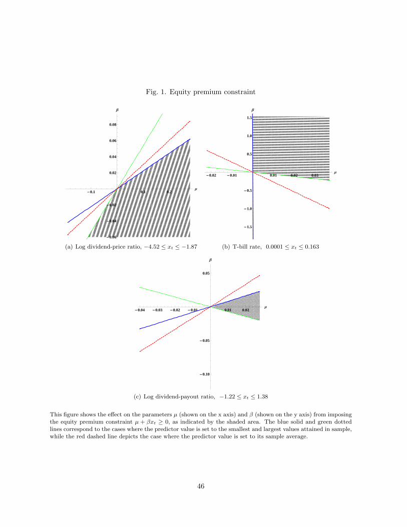
Fig. 1. Equity premium constraint

-0.1 0.1 0.2Μ

-0.06

-0.04

-0.02

0.02

0.04

0.06

0.08

Β

(a) Log dividend-price ratio, −4.52 ≤ xt ≤ −1.87

-0.02 -0.01 0.01 0.02 0.03Μ

-1.5

-1.0

-0.5

0.5

1.0

1.5

Β

(b) T-bill rate, 0.0001 ≤ xt ≤ 0.163

-0.04 -0.03 -0.02 -0.01 0.01 0.02Μ

-0.10

-0.05

0.05

Β

(c) Log dividend-payout ratio, −1.22 ≤ xt ≤ 1.38

This figure shows the effect on the parameters µ (shown on the x axis) and β (shown on the y axis) from imposingthe equity premium constraint µ + βxt ≥ 0, as indicated by the shaded area. The blue solid and green dottedlines correspond to the cases where the predictor value is set to the smallest and largest values attained in sample,while the red dashed line depicts the case where the predictor value is set to its sample average.

46

Fig. 2. Comparison of in-sample fitted values and out-of-sample forecast under the equitypremium constraint and the truncation approach

Exc

ess

retu

rns

(per

cent

age

poin

ts)

1920 1925 1930 1935 1940 1945 1950

−0.4

−0.2

0

0.2

0.4

0.6

0.8

1

1.2

1.4

1.6CT truncated (in−sample fitted values)Equity premium constrained (in−sample fitted values)CT truncated (out−of−sample forecast)Equity premium constrained (out−of−sample forecast)

out of samplein sample

This figure compares the in-sample fitted values and out-of-sample predicted excess return for January 1947 underthe equity premium constraint versus under the truncation approach of Campbell and Thompson (2008, labeledCT truncated). We regress excess returns (rt+1) on an intercept and the lagged log dividend-price ratio, xt overthe period January 1927–December 1946: rt+1 = µ + βxt + εt+1. Estimates from this model are then used togenerate in-sample fitted values as well as a one-step out-of-sample forecast of excess returns for January 1947.The equity premium constrained model imposes that rτ+1|t =

∫(µ+βxτ )p(µ, β| Dt)dµdβ > 0, for τ = 1, ..., t and

information set Dt.

47

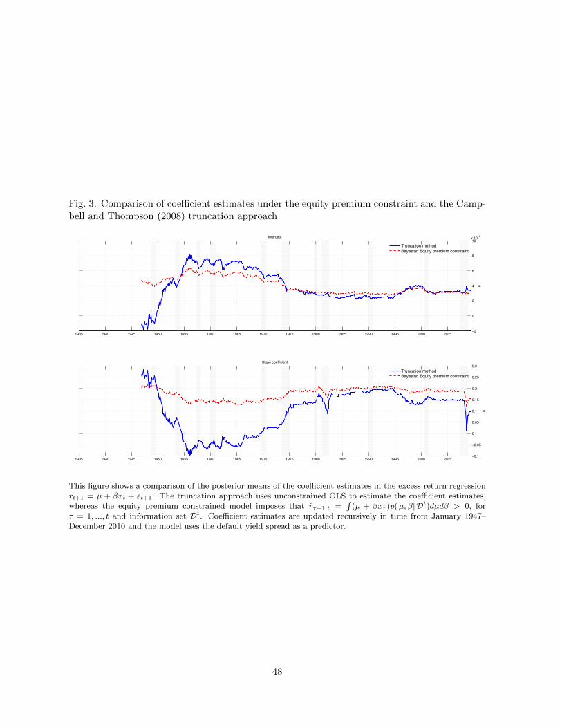
Fig. 3. Comparison of coefficient estimates under the equity premium constraint and the Camp-bell and Thompson (2008) truncation approach

µ

Intercept

1935 1940 1945 1950 1955 1960 1965 1970 1975 1980 1985 1990 1995 2000 2005−2

0

2

4

6

8

10x 10

−3

Truncation method

Bayesian Equity premium constraint

β

Slope coefficient

1935 1940 1945 1950 1955 1960 1965 1970 1975 1980 1985 1990 1995 2000 2005−0.1

−0.05

0

0.05

0.1

0.15

0.2

0.25

0.3

Truncation method

Bayesian Equity premium constraint

This figure shows a comparison of the posterior means of the coefficient estimates in the excess return regressionrt+1 = µ + βxt + εt+1. The truncation approach uses unconstrained OLS to estimate the coefficient estimates,whereas the equity premium constrained model imposes that rτ+1|t =

∫(µ + βxτ )p(µ, β| Dt)dµdβ > 0, for

τ = 1, ..., t and information set Dt. Coefficient estimates are updated recursively in time from January 1947–December 2010 and the model uses the default yield spread as a predictor.

48

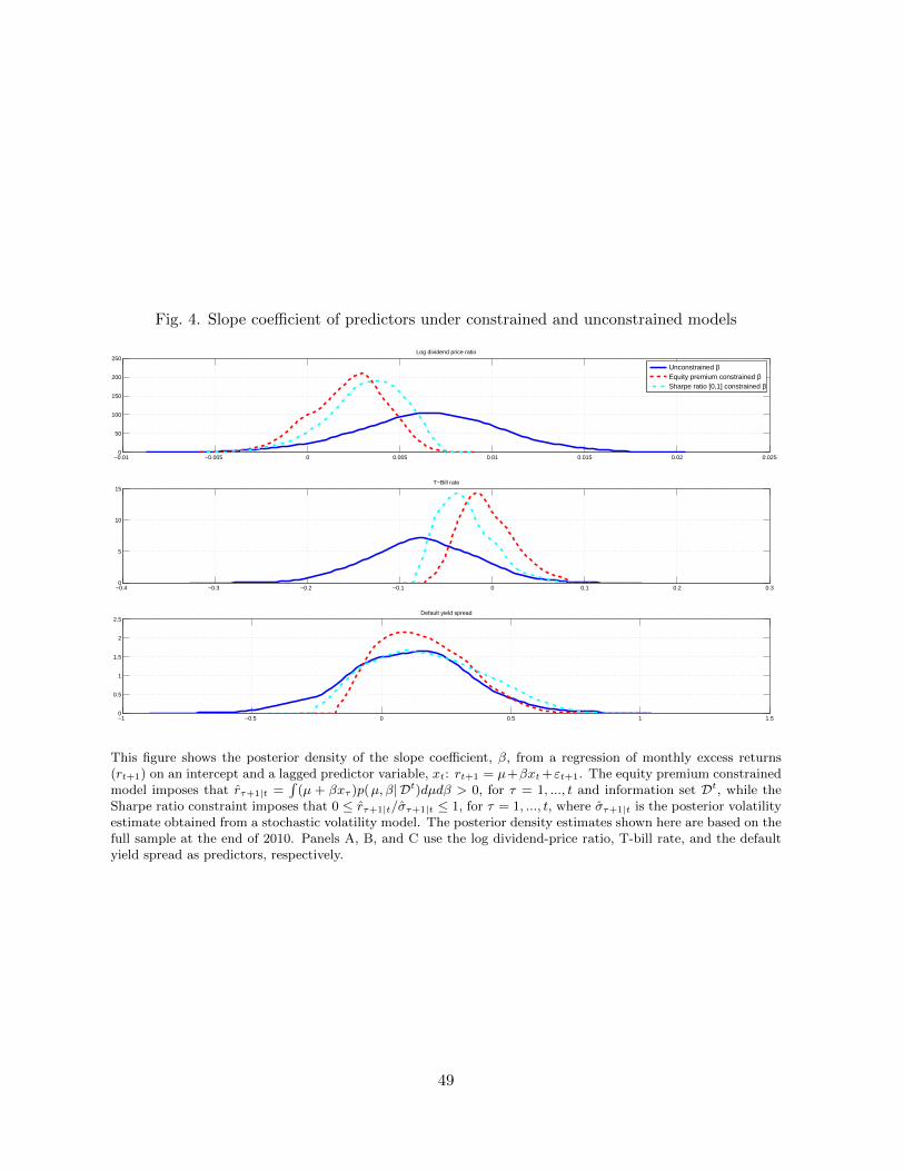
Fig. 4. Slope coefficient of predictors under constrained and unconstrained models

−0.01 −0.005 0 0.005 0.01 0.015 0.02 0.0250

50

100

150

200

250Log dividend price ratio

Unconstrained βEquity premium constrained βSharpe ratio [0,1] constrained β

−0.4 −0.3 −0.2 −0.1 0 0.1 0.2 0.30

5

10

15T−Bill rate

−1 −0.5 0 0.5 1 1.50

0.5

1

1.5

2

2.5Default yield spread

This figure shows the posterior density of the slope coefficient, β, from a regression of monthly excess returns(rt+1) on an intercept and a lagged predictor variable, xt: rt+1 = µ+βxt+εt+1. The equity premium constrainedmodel imposes that rτ+1|t =

∫(µ + βxτ )p(µ, β| Dt)dµdβ > 0, for τ = 1, ..., t and information set Dt, while the

Sharpe ratio constraint imposes that 0 ≤ rτ+1|t/στ+1|t ≤ 1, for τ = 1, ..., t, where στ+1|t is the posterior volatilityestimate obtained from a stochastic volatility model. The posterior density estimates shown here are based on thefull sample at the end of 2010. Panels A, B, and C use the log dividend-price ratio, T-bill rate, and the defaultyield spread as predictors, respectively.

49

Fig. 5. Posterior density of the equity premium under constrained and unconstrained models(Dividend-price ratio)

−0.015 −0.01 −0.005 0 0.005 0.01 0.015 0.02 0.025 0.030

50

100

150

200

250

300mean

Unconstrained

Equity premium constrained

Sharpe ratio [0,1] constrained

−0.015 −0.01 −0.005 0 0.005 0.01 0.015 0.02 0.025 0.030

50

100

150

200

250

300mean − 2 std. dev.

−0.015 −0.01 −0.005 0 0.005 0.01 0.015 0.02 0.025 0.030

50

100

150

200

250

300mean + 2 std. dev.

Log dividend price ratio − ψ = 2.5, v0=0.1

This figure shows the posterior density of the equity premium as a function of the log dividend-price ratio,µ + βxT , where xT is set at the sample mean of the log dividend-price ratio x (top window), x − 2st.dev (x)(middle window), and x + 2st.dev (x) (bottom window). The equity premium constrained model imposes thatrτ+1|t =

∫(µ+βxτ )p(µ, β| Dt)dµdβ > 0, for τ = 1, ..., t and information set Dt, while the Sharpe ratio constraint

imposes that 0 ≤ rτ+1|t/στ+1|t ≤ 1, for τ = 1, ..., t, where στ+1|t is the posterior volatility estimate obtained froma stochastic volatility model. All posterior density estimates are based on the full data sample as of end-2010.

50

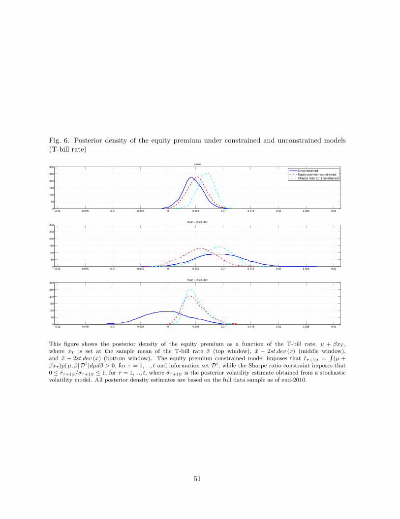
Fig. 6. Posterior density of the equity premium under constrained and unconstrained models(T-bill rate)

−0.02 −0.015 −0.01 −0.005 0 0.005 0.01 0.015 0.02 0.025 0.030

50

100

150

200

250

300mean

Unconstrained

Equity premium constrained

Sharpe ratio [0,1] constrained

−0.02 −0.015 −0.01 −0.005 0 0.005 0.01 0.015 0.02 0.025 0.030

50

100

150

200

250

300mean − 2 std. dev.

−0.02 −0.015 −0.01 −0.005 0 0.005 0.01 0.015 0.02 0.025 0.030

50

100

150

200

250

300mean + 2 std. dev.

T−Bill rate − ψ = 2.5, v0=0.1

This figure shows the posterior density of the equity premium as a function of the T-bill rate, µ + βxT ,where xT is set at the sample mean of the T-bill rate x (top window), x − 2st.dev (x) (middle window),and x + 2st.dev (x) (bottom window). The equity premium constrained model imposes that rτ+1|t =

∫(µ +

βxτ )p(µ, β| Dt)dµdβ > 0, for τ = 1, ..., t and information set Dt, while the Sharpe ratio constraint imposes that0 ≤ rτ+1|t/στ+1|t ≤ 1, for τ = 1, ..., t, where στ+1|t is the posterior volatility estimate obtained from a stochasticvolatility model. All posterior density estimates are based on the full data sample as of end-2010.

51

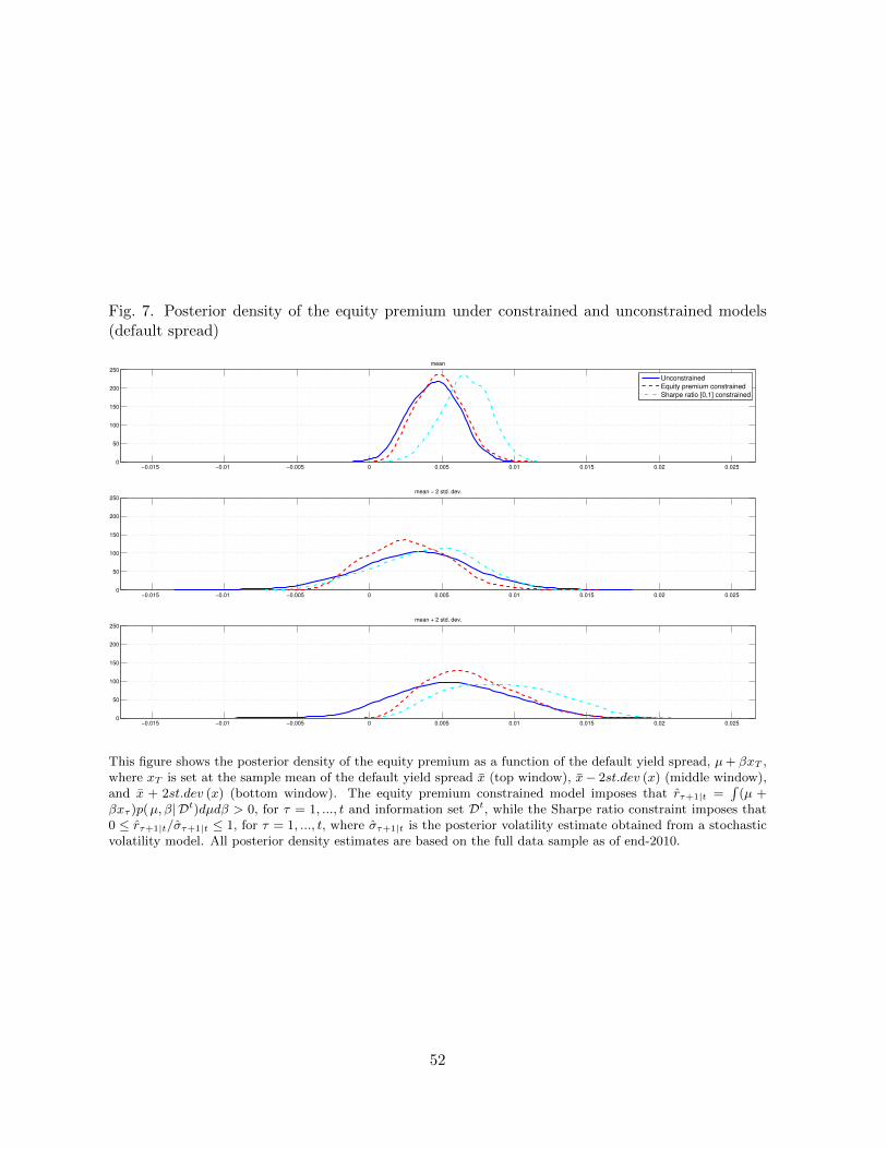
Fig. 7. Posterior density of the equity premium under constrained and unconstrained models(default spread)

−0.015 −0.01 −0.005 0 0.005 0.01 0.015 0.02 0.0250

50

100

150

200

250mean

Unconstrained

Equity premium constrained

Sharpe ratio [0,1] constrained

−0.015 −0.01 −0.005 0 0.005 0.01 0.015 0.02 0.0250

50

100

150

200

250mean − 2 std. dev.

−0.015 −0.01 −0.005 0 0.005 0.01 0.015 0.02 0.0250

50

100

150

200

250mean + 2 std. dev.

Default yield spread − ψ = 2.5, v0=0.1

This figure shows the posterior density of the equity premium as a function of the default yield spread, µ+ βxT ,where xT is set at the sample mean of the default yield spread x (top window), x− 2st.dev (x) (middle window),and x + 2st.dev (x) (bottom window). The equity premium constrained model imposes that rτ+1|t =

∫(µ +

βxτ )p(µ, β| Dt)dµdβ > 0, for τ = 1, ..., t and information set Dt, while the Sharpe ratio constraint imposes that0 ≤ rτ+1|t/στ+1|t ≤ 1, for τ = 1, ..., t, where στ+1|t is the posterior volatility estimate obtained from a stochasticvolatility model. All posterior density estimates are based on the full data sample as of end-2010.

52

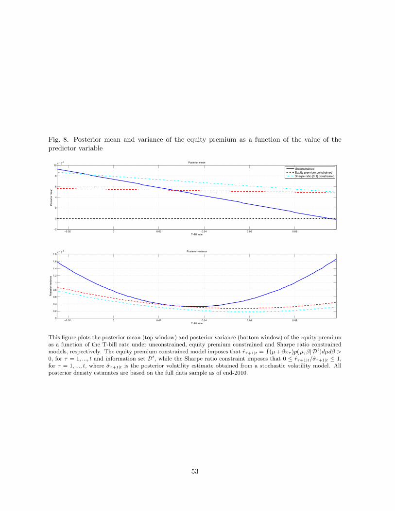
Fig. 8. Posterior mean and variance of the equity premium as a function of the value of thepredictor variable

−0.02 0 0.02 0.04 0.06 0.08−2

0

2

4

6

8

10x 10

−3

T−Bill rate

Po

ste

rio

r m

ean

Posterior mean

Unconstrained

Equity premium constrained

Sharpe ratio [0,1] constrained

−0.02 0 0.02 0.04 0.06 0.080

0.2

0.4

0.6

0.8

1

1.2

1.4

1.6

1.8x 10

−5 Posterior variance

T−Bill rate

Po

ste

rio

r va

ria

nce

This figure plots the posterior mean (top window) and posterior variance (bottom window) of the equity premiumas a function of the T-bill rate under unconstrained, equity premium constrained and Sharpe ratio constrainedmodels, respectively. The equity premium constrained model imposes that rτ+1|t =

∫(µ+βxτ )p(µ, β| Dt)dµdβ >

0, for τ = 1, ..., t and information set Dt, while the Sharpe ratio constraint imposes that 0 ≤ rτ+1|t/στ+1|t ≤ 1,for τ = 1, ..., t, where στ+1|t is the posterior volatility estimate obtained from a stochastic volatility model. Allposterior density estimates are based on the full data sample as of end-2010.

53

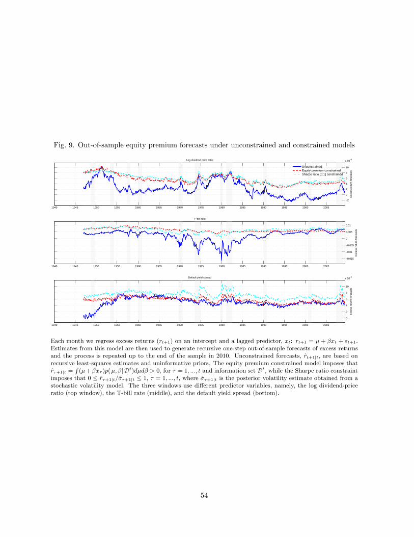
Fig. 9. Out-of-sample equity premium forecasts under unconstrained and constrained models

Exc

ess

retu

rn fo

reca

sts

Log dividend price ratio

1940 1945 1950 1955 1960 1965 1970 1975 1980 1985 1990 1995 2000 2005

−2

0

2

4

6

8

10

x 10−3

UnconstrainedEquity premium constrainedSharpe ratio [0,1] constrained

Exc

ess

retu

rn fo

reca

sts

T−Bill rate

1940 1945 1950 1955 1960 1965 1970 1975 1980 1985 1990 1995 2000 2005

−0.015

−0.01

−0.005

0

0.005

0.01

Exc

ess

retu

rn fo

reca

sts

Default yield spread

1940 1945 1950 1955 1960 1965 1970 1975 1980 1985 1990 1995 2000 2005

0

2

4

6

8

10

x 10−3

Each month we regress excess returns (rt+1) on an intercept and a lagged predictor, xt: rt+1 = µ + βxt + εt+1.Estimates from this model are then used to generate recursive one-step out-of-sample forecasts of excess returnsand the process is repeated up to the end of the sample in 2010. Unconstrained forecasts, rt+1|t, are based onrecursive least-squares estimates and uninformative priors. The equity premium constrained model imposes thatrτ+1|t =

∫(µ+βxτ )p(µ, β| Dt)dµdβ > 0, for τ = 1, ..., t and information set Dt, while the Sharpe ratio constraint

imposes that 0 ≤ rτ+1|t/στ+1|t ≤ 1, τ = 1, ..., t, where στ+1|t is the posterior volatility estimate obtained from astochastic volatility model. The three windows use different predictor variables, namely, the log dividend-priceratio (top window), the T-bill rate (middle), and the default yield spread (bottom).

54

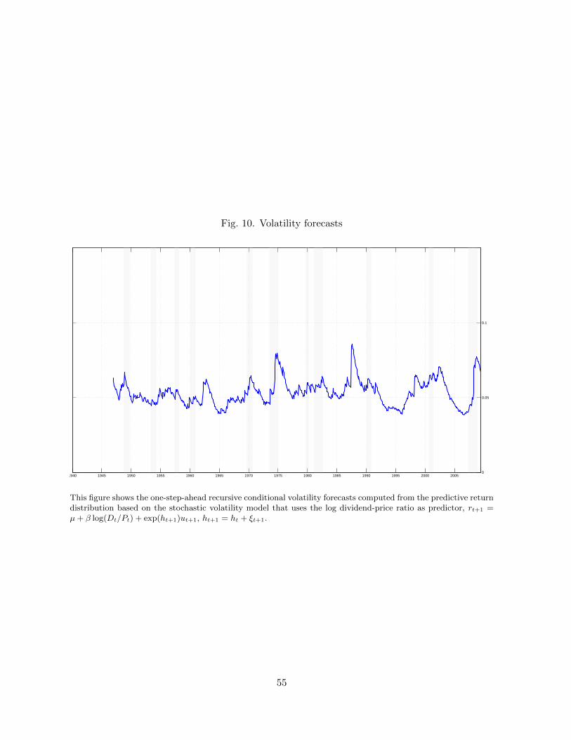
Fig. 10. Volatility forecasts

1940 1945 1950 1955 1960 1965 1970 1975 1980 1985 1990 1995 2000 20050

0.05

0.1

This figure shows the one-step-ahead recursive conditional volatility forecasts computed from the predictive returndistribution based on the stochastic volatility model that uses the log dividend-price ratio as predictor, rt+1 =µ+ β log(Dt/Pt) + exp(ht+1)ut+1, ht+1 = ht + ξt+1.

55

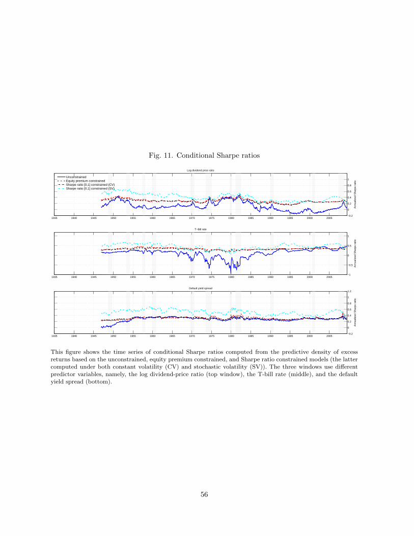
Fig. 11. Conditional Sharpe ratios

Ann

ualiz

ed S

harp

e ra

tio

Log dividend price ratio

1935 1940 1945 1950 1955 1960 1965 1970 1975 1980 1985 1990 1995 2000 2005−0.2

0

0.2

0.4

0.6

0.8

1UnconstrainedEquity premium constrainedSharpe ratio [0,1] constrained (CV)Sharpe ratio [0,1] constrained (SV)

Ann

ualiz

ed S

harp

e ra

tio

T−Bill rate

1935 1940 1945 1950 1955 1960 1965 1970 1975 1980 1985 1990 1995 2000 2005−1

−0.5

0

0.5

1

Ann

ualiz

ed S

harp

e ra

tio

Default yield spread

1935 1940 1945 1950 1955 1960 1965 1970 1975 1980 1985 1990 1995 2000 2005−0.2

0

0.2

0.4

0.6

0.8

1

1.2

This figure shows the time series of conditional Sharpe ratios computed from the predictive density of excessreturns based on the unconstrained, equity premium constrained, and Sharpe ratio constrained models (the lattercomputed under both constant volatility (CV) and stochastic volatility (SV)). The three windows use differentpredictor variables, namely, the log dividend-price ratio (top window), the T-bill rate (middle), and the defaultyield spread (bottom).

56

Fig. 12. Posterior probability intervals for the parameters of the return prediction model

1965 1970 1975 1980

0.005

0.01

0.015

0.02

0.025

0.03

0.035

0.04

0.045

0.05

0.055

Unconstrained µ

1965 1970 1975 1980

0.005

0.01

0.015

0.02

0.025

0.03

0.035

0.04

0.045

0.05

0.055

Equity premium constrained µ

1965 1970 1975 1980

−1

−0.8

−0.6

−0.4

−0.2

0

Unconstrained β

1965 1970 1975 1980

−1

−0.8

−0.6

−0.4

−0.2

0

Equity premium constrained β

Each month we update the posterior density of the parameters µ, β of the return prediction model rt+1 =µ + βxt + εt+1, where xt is the T-bill rate and rt+1 is the return on the S&P 500 index, measured in excessof the T-bill rate. We then compute posterior probability intervals for these parameter estimates. Windows tothe left report the (2.5, 97.5) percentile posterior probability intervals for the parameters of the unconstrainedmodel, while windows to the right show results for the equity-premium constrained model. The equity premiumconstrained model imposes that rτ+1|t =

∫(µ + βxτ )p(µ, β|Dt)dµdβ > 0 for all τ = 1, ..., t and information set

Dt. All density estimates are updated recursively through time.

57

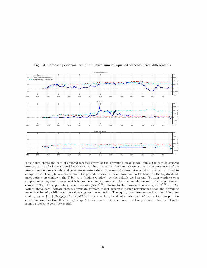
Fig. 13. Forecast performance: cumulative sum of squared forecast error differentials

Cum

ulat

ive

SS

E d

iffer

ence

Log dividend price ratio

1940 1945 1950 1955 1960 1965 1970 1975 1980 1985 1990 1995 2000 2005−0.01

−0.005

0

0.005

0.01

0.015

0.02

UnconstrainedEquity premium constrainedSharpe ratio [0,1] constrained

Cum

ulat

ive

SS

E d

iffer

ence

T−Bill rate

1940 1945 1950 1955 1960 1965 1970 1975 1980 1985 1990 1995 2000 2005−0.01

−0.005

0

0.005

0.01

0.015

0.02

Cum

ulat

ive

SS

E d

iffer

ence

Default yield spread

1940 1945 1950 1955 1960 1965 1970 1975 1980 1985 1990 1995 2000 2005−0.01

−0.005

0

0.005

0.01

0.015

0.02

This figure shows the sum of squared forecast errors of the prevailing mean model minus the sum of squaredforecast errors of a forecast model with time-varying predictors. Each month we estimate the parameters of theforecast models recursively and generate one-step-ahead forecasts of excess returns which are in turn used tocompute out-of-sample forecast errors. This procedure uses univariate forecast models based on the log dividend-price ratio (top window), the T-bill rate (middle window), or the default yield spread (bottom window) or asimple prevailing mean model which is our benchmark. We then plot the cumulative sum of squared forecasterrors (SSEt) of the prevailing mean forecasts (SSEPMt ) relative to the univariate forecasts, SSEPMt − SSEt.Values above zero indicate that a univariate forecast model generates better performance than the prevailingmean benchmark, while negative values suggest the opposite. The equity premium constrained model imposesthat rτ+1|t =

∫(µ + βxτ )p(µ, β| Dt)dµdβ > 0, for τ = 1, ..., t and information set Dt, while the Sharpe ratio

constraint imposes that 0 ≤ rτ+1|t/στ+1|t ≤ 1, for τ = 1, ..., t, where στ+1|t is the posterior volatility estimatefrom a stochastic volatility model.

58

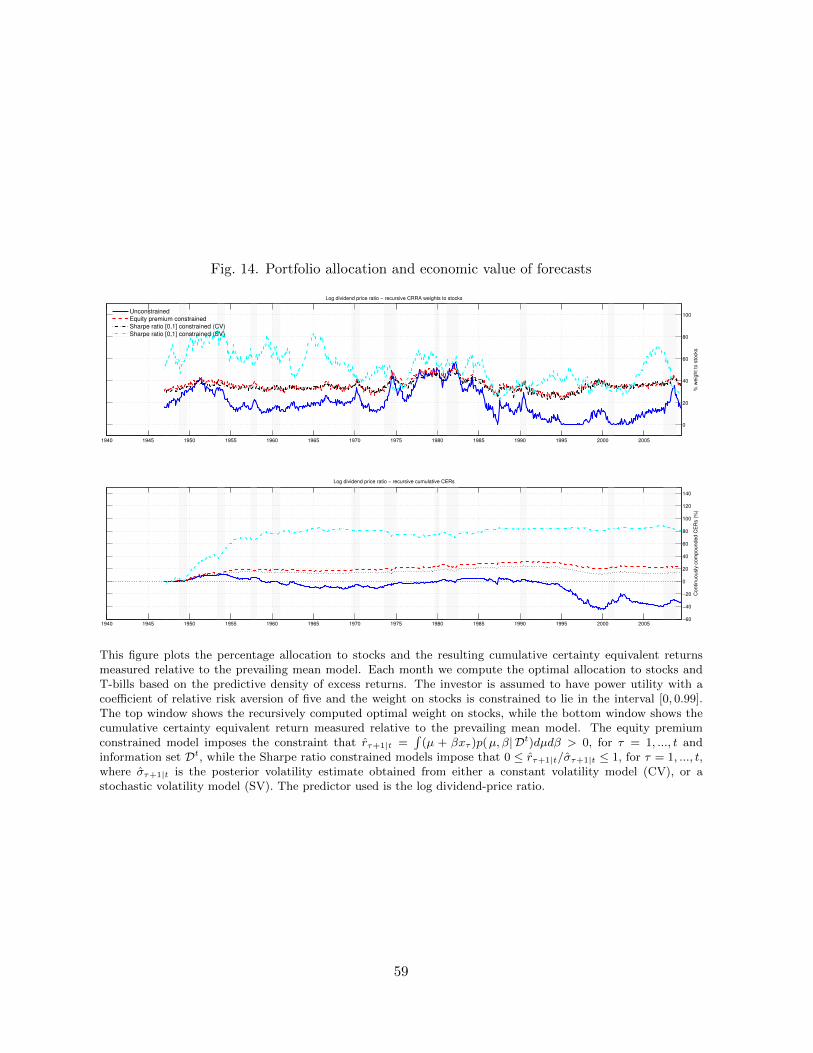
Fig. 14. Portfolio allocation and economic value of forecasts

% w

eig

ht

to s

tocks

Log dividend price ratio − recursive CRRA weights to stocks

1940 1945 1950 1955 1960 1965 1970 1975 1980 1985 1990 1995 2000 2005

0

20

40

60

80

100Unconstrained

Equity premium constrained

Sharpe ratio [0,1] constrained (CV)

Sharpe ratio [0,1] constrained (SV)

Co

ntin

uo

usly

com

po

und

ed

CE

Rs (

%)

Log dividend price ratio − recursive cumulative CERs

1940 1945 1950 1955 1960 1965 1970 1975 1980 1985 1990 1995 2000 2005−60

−40

−20

0

20

40

60

80

100

120

140

This figure plots the percentage allocation to stocks and the resulting cumulative certainty equivalent returnsmeasured relative to the prevailing mean model. Each month we compute the optimal allocation to stocks andT-bills based on the predictive density of excess returns. The investor is assumed to have power utility with acoefficient of relative risk aversion of five and the weight on stocks is constrained to lie in the interval [0, 0.99].The top window shows the recursively computed optimal weight on stocks, while the bottom window shows thecumulative certainty equivalent return measured relative to the prevailing mean model. The equity premiumconstrained model imposes the constraint that rτ+1|t =

∫(µ + βxτ )p(µ, β| Dt)dµdβ > 0, for τ = 1, ..., t and

information set Dt, while the Sharpe ratio constrained models impose that 0 ≤ rτ+1|t/στ+1|t ≤ 1, for τ = 1, ..., t,where στ+1|t is the posterior volatility estimate obtained from either a constant volatility model (CV), or astochastic volatility model (SV). The predictor used is the log dividend-price ratio.

59

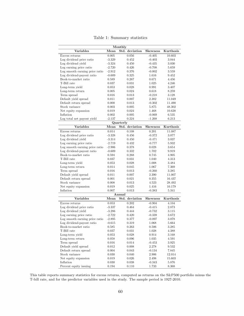
Table 1: Summary statistics

Monthly

Variables Mean Std. deviation Skewness Kurthosis

Excess returns 0.005 0.056 -0.405 10.603Log dividend price ratio -3.329 0.452 -0.403 3.044Log dividend yield -3.324 0.450 -0.435 3.030Log earning price ratio -2.720 0.426 -0.708 5.659Log smooth earning price ratio -2.912 0.376 -0.002 3.559Log dividend-payout ratio -0.609 0.325 1.616 9.452Book-to-market ratio 0.589 0.267 0.671 4.456T-Bill rate 0.037 0.031 1.025 4.246Long-term yield 0.053 0.028 0.991 3.407Long-term return 0.005 0.024 0.618 8.259Term spread 0.016 0.013 -0.218 3.128Default yield spread 0.011 0.007 2.382 11.049Default return spread 0.000 0.013 -0.302 11.490Stock variance 0.003 0.005 5.875 48.302Net equity expansion 0.019 0.024 1.468 10.638Inflation 0.002 0.005 -0.069 6.535Log total net payout yield -2.137 0.224 -1.268 6.213

Quarterly

Variables Mean Std. deviation Skewness Kurthosis

Excess returns 0.014 0.108 0.201 11.087Log dividend price ratio -3.328 0.456 -0.372 3.077Log dividend yield -3.314 0.450 -0.471 3.037Log earning price ratio -2.719 0.432 -0.777 5.932Log smooth earning price ratio -2.906 0.378 0.028 3.654Log dividend-payout ratio -0.609 0.332 1.702 9.919Book-to-market ratio 0.594 0.268 0.745 4.905T-Bill rate 0.037 0.031 1.040 4.313Long-term yield 0.053 0.028 1.008 3.484Long-term return 0.014 0.045 1.067 7.369Term spread 0.016 0.013 -0.260 3.285Default yield spread 0.011 0.007 2.390 11.007Default return spread 0.001 0.021 0.355 16.437Stock variance 0.008 0.013 4.523 28.492Net equity expansion 0.019 0.025 1.416 10.179Inflation 0.007 0.013 -0.383 5.341

Annual

Variables Mean Std. deviation Skewness Kurthosis

Excess returns 0.053 0.202 -0.904 4.104Log dividend price ratio -3.337 0.464 -0.415 2.873Log dividend yield -3.286 0.444 -0.732 3.115Log earning price ratio -2.722 0.420 -0.339 3.672Log smooth earning price ratio -2.895 0.377 -0.097 3.078Log dividend-payout ratio -0.615 0.319 1.068 5.664Book-to-market ratio 0.585 0.263 0.506 3.285T-Bill rate 0.037 0.031 1.028 4.388Long-term yield 0.053 0.028 0.914 3.168Long-term return 0.058 0.096 1.035 4.591Term spread 0.016 0.014 -0.453 3.925Default yield spread 0.012 0.008 2.278 9.532Default return spread 0.004 0.043 -0.134 7.845Stock variance 0.030 0.040 2.906 12.014Net equity expansion 0.019 0.026 2.498 15.603Inflation 0.030 0.038 -0.343 5.876Percent equity issuing 0.194 0.110 1.733 8.368

This table reports summary statistics for excess returns, computed as returns on the S&P500 portfolio minus theT-bill rate, and for the predictor variables used in the study. The sample period is 1927-2010.

60

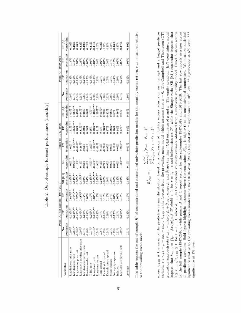
Tab

le2:

Ou

t-of

-sam

ple

fore

cast

per

form

ance

(mon

thly

)

PanelA:full

sample

(1947-2010)

PanelB:1947-1978

PanelC:1979-2010

Variables

No

CT

EP

SR

[0,1]

No

CT

EP

SR

[0,1]

No

CT

EP

SR

[0,1]

constra

int

truncation

constra

int

constra

int

constra

int

truncation

constra

int

constra

int

constra

int

truncation

constra

int

constra

int

Log

div

iden

dpri

cera

tio

0.10

%*

0.25%**

0.64%***

0.49%**

1.01

%**

1.01%

**

1.31%***

1.03%**

-0.5

9%

-0.33%

0.14%

0.08%

Log

div

iden

dyie

ld-0

.16%

**0.31%**

0.76%***

0.54%**

0.97

%***

1.18%***

1.55%***

1.05%**

-1.0

1%

-0.35%

0.17%

0.16%

Log

earn

ing

pri

cera

tio

-1.3

8%

*-0.45%**

0.25%*

0.30%*

-1.1

7%*

-0.80%*

0.18%

0.43%

-1.5

4%

-0.19%

0.31%

0.20%

Log

smooth

earn

ing

pri

cera

tio

-0.7

9%

*0.07%**

0.48%**

0.47%**

-0.1

4%*

0.26%*

0.81%**

0.94%**

-1.2

8%

-0.07%

0.23%

0.12%

Log

div

iden

d-p

ayou

tra

tio

-1.5

7%

-1.29%

-0.12%

0.03%

-2.6

4%-2

.64%

-0.32%

0.23%

-0.7

6%

-0.26%

0.03%

-0.12%

Book-t

o-m

ark

etra

tio

-1.4

0%

-0.88%

0.02%

0.04%

-0.4

2%-0

.49%

0.08%

0.06%

-2.1

4%

-1.17%

-0.03%

0.02%

T-B

ill

rate

0.01

%*

0.20%*

0.10%

0.54%**

1.50

%**

1.21%

**

0.28%

1.40%

***

-1.1

1%

-0.57%

-0.04%

-0.11%

Lon

g-t

erm

yie

ld-0

.94%

*0.20%**

0.31%**

0.55%***

-0.4

7%*

1.02%**

0.78%**

1.43%***

-1.3

0%

-0.42%

-0.04%

-0.11%

Lon

g-t

erm

retu

rn-0

.74%

-0.62%

0.19%

0.53%**

-1.9

0%-1.61%

0.31%

1.25%**

0.1

3%

0.1

3%

0.1

0%

-0.0

2%T

erm

spre

ad

0.06

%0.0

4%0.

05%

0.24%*

0.41

%0.

41%

0.14

%0.53%*

-0.2

0%

-0.2

3%-0.02%

0.02%

Def

ault

yie

ldsp

read

-0.1

9%

-0.18%

0.18%

-0.08%

-0.2

4%-0.22%

0.53%**

0.22%

-0.1

5%

-0.1

5%-0.07%

-0.3

1%

Def

ault

retu

rnsp

read

-0.2

4%

-0.3

9%0.15%

-0.3

0%-0

.97%

-0.9

7%0.37%

-0.42%

0.3

2%

0.0

5%

0.0

0%

-0.2

0%S

tock

vari

an

ce0.

24%

0.1

1%-0

.17%

-0.2

9%-0

.07%

-0.0

7%0.36%*

0.08%

0.4

8%

0.2

4%

-0.5

7%

-0.5

6%

Net

equ

ity

exp

an

sion

-0.7

9%

-0.77%

-0.01%

-0.08%

0.08

%0.12%

0.15%

0.03

%-1

.45%

-1.44%

-0.13%

-0.16%

Infl

atio

n-0

.13%

-0.1

3%0.07%

-0.12%

-0.0

5%-0

.05%

0.14%

0.36%

-0.2

0%

-0.2

0%0.02%

-0.4

7%

Log

tota

ln

etp

ayou

tyie

ld-0

.49%

*0.09%*

0.18%

-0.01%

1.44

%***

1.21%

**

0.45%

*0.

25%

-1.9

7%

-0.76%

0.00%

-0.17%

Ave

rage

-0.5

3%

-0.22%

0.19%

0.18%

-0.1

7%-0.03%

0.44%

0.55%

-0.8

0%

-0.36%

0.01%

-0.10%

This

table

rep

ort

sth

eout-

of-

sam

pleR

2of

unco

nst

rain

edand

const

rain

eduniv

ari

ate

pre

dic

tion

model

sfo

rth

em

onth

lyex

cess

retu

rn,r t

+1,

mea

sure

dre

lati

ve

toth

epre

vailin

gm

ean

model

:

R2 OoS

=1−

∑ t−1

τ=t−

1(rt+

1−r t

+1|t

)2

∑ t−1

τ=t−

1(rt+

1−r t

+1|t

)2,

wher

er t

+1|t

isth

em

ean

of

the

pre

dic

tive

retu

rndis

trib

uti

on

base

don

are

gre

ssio

nof

month

lyex

cess

retu

rns

on

an

inte

rcep

tand

ala

gged

pre

dic

tor

vari

able

,xt:r t

+1

=µ

+βxt

+ε t

+1.r t

+1|t

isth

efo

reca

stfr

om

the

pre

vailin

gm

ean

model

whic

hass

um

esth

atβ

=0.

The

Cam

pb

ell

and

Thom

pso

n(C

T)

trunca

tion

appro

ach

setsr t

+1|t

=m

ax(0,µt+βtxt),

wher

eµt

andβt

are

the

tim

et

OL

Ses

tim

ate

sofµ

andβ

.T

he

equit

ypre

miu

m(E

P)

const

rain

edm

odel

imp

ose

sth

atr τ

+1|t

=∫ (µ

+βxτ)p

(µ,β|D

t)dµdβ>

0,

forτ

=1,...,t

and

info

rmati

on

setDt,

while

the

Sharp

era

tio

(SR

[0,1

])co

nst

rain

tim

pose

sth

at

0≤r τ

+1|t/στ+1|t≤

1,

forτ

=1,...,t

,w

her

eστ+1|t

isth

ep

ost

erio

rvola

tility

esti

mate

obta

ined

from

ast

och

ast

icvola

tility

model

.P

anel

Ash

ows

resu

lts

for

the

full

sam

ple

(1947-2

010),

while

panel

sB

and

Cre

port

resu

lts

for

the

subsa

mple

s1947-1

978

and

1979-2

010.

The

last

row

rep

ort

sav

erages

acr

oss

all

pre

dic

tor

vari

able

s.B

old

figure

shig

hlight

inst

ance

sw

her

eth

eco

nst

rain

edR

2 OoS

ishig

her

than

its

unco

nst

rain

edco

unte

rpart

.W

em

easu

rest

ati

stic

al

signifi

cance

rela

tive

toth

epre

vailin

gm

ean

model

usi

ng

the

Cla

rk-W

est

(2007)

test

stati

stic

.*

signifi

cance

at

10%

level

;**

signifi

cance

at

5%

level

;***

signifi

cance

at

1%

level

.

61

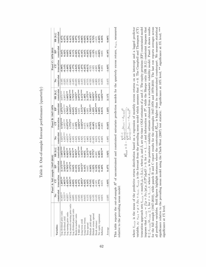
Tab

le3:

Ou

t-of

-sam

ple

fore

cast

per

form

ance

(qu

arte

rly)

PanelA:full

sample

(1947-2010)

PanelB:1947-1978

PanelC:1979-2010

Variables

No

CT

EP

SR

[0,1]

No

CT

EP

SR

[0,1]

No

CT

EP

SR

[0,1]

constra

int

truncation

constra

int

constra

int

constra

int

truncation

constra

int

constra

int

constra

int

truncation

constra

int

constra

int

Log

div

iden

dpri

cera

tio

-0.1

6%**

1.20%**

2.11%***

1.68%***

3.22

%**

*3.72%***

4.27%***

3.0

7%

***

-3.1

0%-0.98%

0.24%

0.47%

Log

div

iden

dyie

ld0.

75%

**

1.86%**

2.04%***

1.88%***

4.19

%**

*4.1

8%**

*4.

04%

***

3.3

8%

***

-2.2

2%-0.14%

0.32%

0.57%

Log

earn

ing

pri

cera

tio

-6.3

3%*

-2.42%**

0.70%**

0.92%**

-4.6

5%**

-3.37%**

0.78%*

1.60%**

-7.7

8%-1.60%

0.63%

0.33%

Log

smoot

hea

rnin

gpri

cera

tio

-3.5

8%**

0.50%**

1.57%**

1.60%**

-0.8

0%**

1.77%**

3.03%**

2.96%***

-5.9

8%-0.60%

0.30%

0.41%

Log

div

iden

d-p

ayou

tra

tio

-3.6

9%-3.02%

0.04%

0.81%**

-5.1

6%-5

.16%

-0.04%

1.75%***

-2.4

2%-1.17%

0.11%

0.00%

Book

-to-

mar

ket

rati

o-6

.24%

-3.16%

-0.15%

0.96%*

-1.6

4%-1.22%

0.04%

1.64%*

-10.

23%

-4.84%

-0.32%

0.37%

T-B

ill

rate

-0.5

3%0.47%

0.01%

1.87%***

2.40

%2.92%**

0.34%

3.87%***

-3.0

6%-1.65%

-0.27%

0.14%

Lon

g-te

rmyie

ld-2

.70%

0.39%*

0.61%*

1.55%***

-1.8

2%2.32%**

1.51%**

3.41%***

-3.4

5%-1.27%

-0.16%

-0.06%

Lon

g-te

rmre

turn

-0.6

4%-0.32%

0.44%

0.66%

-0.4

1%-0

.41%

0.68%

1.46%

-0.8

4%-0.25%

0.24%

-0.03%

Ter

msp

read

0.11

%0.16%

0.04

%1.21%**

1.06

%1.

06%

0.3

9%2.17%**

-0.7

1%-0.61%

-0.25%

0.38%

Def

ault

yie

ldsp

read

-0.8

2%-0.74%

0.50%

0.42%

-0.9

4%-0.75%

1.79%**

1.49%*

-0.7

2%-0

.72%

-0.62%

-0.51%

Def

ault

retu

rnsp

read

-6.1

4%-5.43%

-1.22%

0.77%*

-11.

02%

-9.48%

-1.33%

0.83%*

-1.9

2%-1

.92%

-1.12%

0.72%

Sto

ckva

rian

ce-0

.14%

-0.1

4%0.12%

-0.2

6%0.

01%

0.01%

1.66%***

1.53%**

-0.2

6%-0

.26%

-1.2

2%

-1.8

1%

Net

equit

yex

pan

sion

-4.9

1%-4.77%

-0.19%

0.29%

-0.4

7%-0.26%

0.28%

0.87%

-8.7

5%-8.68%

-0.60%

-0.20%

Inflat

ion

0.01

%0.

01%

0.40%

0.95%**

-0.2

6%-0

.26%

0.81%

1.63%***

0.2

5%0.

25%

0.05

%0.35%

Ave

rage

-2.3

3%-1.03%

0.47%

1.02%

-1.0

9%-0.33%

1.22%

2.11%

-3.4

1%-1.63%

-0.18%

0.08%

This

table

rep

ort

sth

eout-

of-

sam

pleR

2of

unco

nst

rain

edand

const

rain

eduniv

ari

ate

pre

dic

tion

model

sfo

rth

equart

erly

exce

ssre

turn

,r t

+1,

mea

sure

dre

lati

ve

toth

epre

vailin

gm

ean

model

:

R2 OoS

=1−

∑ t−1

τ=t−

1(rt+

1−r t

+1|t

)2

∑ t−1

τ=t−

1(rt+

1−r t

+1|t

)2,

wher

er t

+1|t

isth

em

ean

of

the

pre

dic

tive

retu

rndis

trib

uti

on

base

don

are

gre

ssio

nof

month

lyex

cess

retu

rns

on

an

inte

rcep

tand

ala

gged

pre

dic

tor

vari

able

,xt:r t

+1

=µ

+βxt

+ε t

+1.r t

+1|t

isth

efo

reca

stfr

om

the

pre

vailin

gm

ean

model

whic

hass

um

esth

atβ

=0.

The

Cam

pb

ell

and

Thom

pso

n(C

T)

trunca

tion

appro

ach

setsr t

+1|t

=m

ax(0,µt+βtxt),

wher

eµt

andβt

are

the

tim

et

OL

Ses

tim

ate

sofµ

andβ

.T

he

equit

ypre

miu

m(E

P)

const

rain

edm

odel

imp

ose

sth

atr τ

+1|t

=∫ (µ

+βxτ)p

(µ,β|D

t)dµdβ>

0,

forτ

=1,...,t

and

info

rmati

on

setDt,

while

the

Sharp

era

tio

(SR

[0,1

])co

nst

rain

tim

pose

sth

at

0≤r τ

+1|t/στ+1|t≤

1,

forτ

=1,...,t

,w

her

eστ+1|t

isth

ep

ost

erio

rvola

tility

esti

mate

obta

ined

from

ast

och

ast

icvola

tility

model

.P

anel

Ash

ows

resu

lts

for

the

full

sam

ple

(1947-2

010),

while

panel

sB

and

Cre

port

resu

lts

for

the

subsa

mple

s1947-1

978

and

1979-2

010.

The

last

row

rep

ort

sav

erages

acr

oss

all

pre

dic

tor

vari

able

s.B

old

figure

shig

hlight

inst

ance

sw

her

eth

eco

nst

rain

edR

2 OoS

ishig

her

than

its

unco

nst

rain

edco

unte

rpart

.W

em

easu

rest

ati

stic

al

signifi

cance

rela

tive

toth

epre

vailin

gm

ean

model

usi

ng

the

Cla

rk-W

est

(2007)

test

stati

stic

.*

signifi

cance

at

10%

level

;**

signifi

cance

at

5%

level

;***

signifi

cance

at

1%

level

.

62

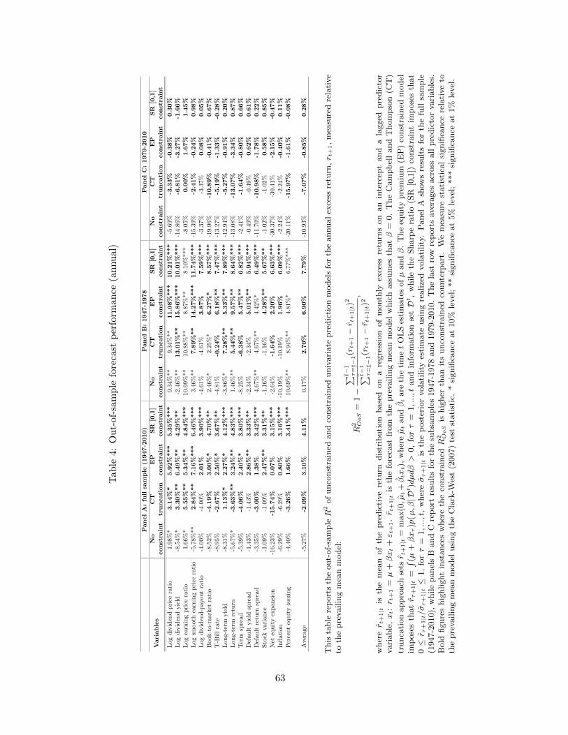
Tab

le4:

Ou

t-of

-sam

ple

fore

cast

per

form

ance

(an

nu

al)

PanelA:full

sample

(1947-2010)

PanelB:1947-1978

PanelC:1979-2010

Variables

No

CT

EP

SR

[0,1]

No

CT

EP

SR

[0,1]

No

CT

EP

SR

[0,1]

constra

int

truncation

constra

int

constra

int

constra

int

truncation

constra

int

constra

int

constra

int

truncation

constra

int

constra

int

Log

div

iden

dpri

cera

tio

1.9

8%

*3.14%*

5.92%***

5.35%***

9.34

%**

9.34

%**

11.98%***

10.21%***

-5.6

9%

-3.33%

-0.38%

0.30%

Log

div

iden

dyie

ld-8

.54%

*3.30%**

6.49%**

4.29%**

-2.4

6%**

13.01%**

15.86%***

10.01%***

-14.8

6%

-6.81%

-3.27%

-1.66%

Log

earn

ing

pri

cera

tio

1.6

6%

*5.55%**

5.34%**

4.84%***

10.9

9%**

10.8

8%**

8.87

%**

8.10

%**

*-8

.05%

0.00%

1.67%

1.45%

Log

smoot

hea

rnin

gpri

cera

tio

-5.7

8%**

2.84%**

7.16%***

6.46%***

3.46

%**

7.89%**

14.27%***

11.74%***

-15.3

9%

-2.41%

-0.24%

0.98%

Log

div

iden

d-p

ayou

tra

tio

-4.0

0%-4

.00%

2.01%

3.90%***

-4.6

1%-4

.61%

3.87%

7.59%***

-3.3

7%

-3.3

7%

0.08%

0.05%

Book

-to-m

arke

tra

tio

-8.5

2%-4.19%

3.00%*

4.70%**

2.46

%*

2.25

%*

6.27%*

8.57%***

-19.9

6%

-10.89%

-0.41%

0.67%

T-B

ill

rate

-8.9

5%-2.67%

2.50%*

3.67%**

-4.8

1%-0.24%

6.18%**

7.47%***

-13.2

7%

-5.19%

-1.33%

-0.28%

Lon

g-te

rmyie

ld-8

.31%

1.13%*

2.27%*

4.12%***

-3.8

6%*

7.28%**

5.33%**

7.89%***

-12.9

4%

-5.27%

-0.91%

0.20%

Lon

g-te

rmre

turn

-5.6

7%*

-3.63%**

3.24%**

4.83%***

1.46

%**

5.44%**

9.57%**

8.64%***

-13.0

8%

-13.07%

-3.34%

0.87%

Ter

msp

read

-5.3

9%-4.06%

2.40%*

3.80%***

-8.2

5%-6.38%

5.47%**

6.82%***

-2.4

1%

-1.64%

-0.80%

0.66%

Def

ault

yie

ldsp

read

-1.4

3%-1

.43%

2.86%**

3.33%**

-2.3

4%-2

.34%

5.01%**

5.94%***

-0.4

9%

-0.4

9%

0.62%

0.61%

Def

ault

retu

rnsp

read

-3.3

5%-3.00%

1.38%

3.42%***

4.67

%**

4.67

%**

4.42

%*

6.49%***

-11.7

0%

-10.98%

-1.78%

0.22%

Sto

ckva

rian

ce-1

.09%

-1.0

9%2.47%**

3.31%**

-1.1

6%-1

.16%

4.28%**

5.67%**

-1.0

2%

-1.0

2%

0.58%

0.85%

Net

equit

yex

pan

sion

-16.2

3%

-15.74%

0.07%

3.15%***

-2.6

4%-1.64%

2.20%

6.63%***

-30.3

7%

-30.4

1%

-2.15%

-0.47%

Inflat

ion

-6.2

9%-6

.29%

0.80%

3.16%***

-10.

19%

-10.

19%

1.96%

6.09%***

-2.2

4%

-2.2

4%

-0.40%

0.11%

Per

cent

equit

yis

suin

g-4

.40%

-3.26%

1.66%

3.41%***

10.6

9%**

8.94

%**

4.81

%*

6.77

%**

*-2

0.1

1%

-15.97%

-1.61%

-0.08%

Ave

rage

-5.2

7%-2.09%

3.10%

4.11%

0.17

%2.70%

6.90%

7.79%

-10.9

3%

-7.07%

-0.85%

0.28%

This

table

rep

ort

sth

eout-

of-

sam

pleR

2of

unco

nst

rain

edand

const

rain

eduniv

ari

ate

pre

dic

tion

model

sfo

rth

eannual

exce

ssre

turn

,r t

+1,

mea

sure

dre

lati

ve

toth

epre

vailin

gm

ean

model

:

R2 OoS

=1−

∑ t−1

τ=t−

1(rt+

1−r t

+1|t

)2

∑ t−1

τ=t−

1(rt+

1−r t

+1|t

)2,

wher

er t

+1|t

isth

em

ean

of

the

pre

dic

tive

retu

rndis

trib

uti

on

base

don

are

gre

ssio

nof

month

lyex

cess

retu

rns

on

an

inte

rcep

tand

ala

gged

pre

dic

tor

vari

able

,xt:r t

+1

=µ

+βxt

+ε t

+1.r t

+1|t

isth

efo

reca

stfr

om

the

pre

vailin

gm

ean

model

whic

hass

um

esth

atβ

=0.

The

Cam

pb

ell

and

Thom

pso

n(C

T)

trunca

tion

appro

ach

setsr t

+1|t

=m

ax(0,µt+βtxt),

wher

eµt

andβt

are

the

tim

et

OL

Ses

tim

ate

sofµ

andβ

.T

he

equit

ypre

miu

m(E

P)

const

rain

edm

odel

imp

ose

sth

atr τ

+1|t

=∫ (µ

+βxτ)p

(µ,β|D

t)dµdβ>

0,

forτ

=1,...,t

and

info

rmati

on

setDt,

while

the

Sharp

era

tio

(SR

[0,1

])co

nst

rain

tim

pose

sth

at

0≤r τ

+1|t/στ+1|t≤

1,

forτ

=1,...,t

,w

her

eστ+1|t

isth

ep

ost

erio

rvola

tility

esti

mate

usi

ng

realize

dvola

tility

.P

anel

Ash

ows

resu

lts

for

the

full

sam

ple

(1947-2

010),

while

panel

sB

and

Cre

port

resu

lts

for

the

subsa

mple

s1947-1

978

and

1979-2

010.

The

last

row

rep

ort

sav

erages

acr

oss

all

pre

dic

tor

vari

able

s.B

old

figure

shig

hlight

inst

ance

sw

her

eth

eco

nst

rain

edR

2 OoS

ishig

her

than

its

unco

nst

rain

edco

unte

rpart

.W

em

easu

rest

ati

stic

al

signifi

cance

rela

tive

toth

epre

vailin

gm

ean

model

usi

ng

the

Cla

rk-W

est

(2007)

test

stati

stic

.*

signifi

cance

at

10%

level

;**

signifi

cance

at

5%

level

;***

signifi

cance

at

1%

level

.

63

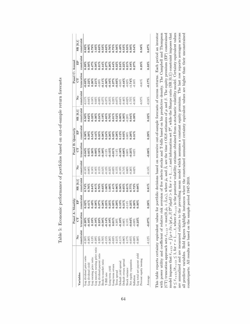
Tab

le5:

Eco

nom

icp

erfo

rman

ceof

por

tfol

ios

bas

edon

out-

of-s

amp

lere

turn

fore

cast

s

PanelA:M

onth

lyPanelB:Quarterly

PanelC:Annual

Variables

No

CT

EP

SR

[0,1]

No

CT

EP

SR

[0,1]

No

CT

EP

SR

[0,1]

constra

int

truncation

constra

int

constra

int

constra

int

truncation

constra

int

constra

int

constra

int

truncation

constra

int

constra

int

Log

div

iden

dpri

cera

tio

-0.2

8%-0.20%

0.32%

0.74%

-0.1

8%-0.04%

0.38%

0.50%

-0.1

1%-0.03%

0.39%

0.92%

Log

div

iden

dyie

ld-0

.26%

-0.10%

0.41%

0.76%

-0.0

8%0.05%

0.39%

0.62%

-0.0

4%0.22%

0.50%

0.90%

Log

earn

ing

pri

cera

tio

0.13%

0.19%

0.49%

0.84%

0.18

%0.26%

0.54%

0.33%

0.18%

0.26%

0.47%

0.79%

Log

smoot

hea

rnin

gp

rice

rati

o-0

.29%

-0.18%

0.38%

0.81%

-0.1

6%0.00%

0.44%

0.36%

0.03%

0.21%

0.58%

1.03%

Log

div

iden

d-p

ayou

tra

tio

0.20%

0.23%

0.37%

0.70%

0.15

%0.18%

0.35%

0.24%

-0.0

9%-0

.09%

0.31%

0.63%

Book

-to-

mar

ket

rati

o-0

.76%

-0.58%

0.28%

0.63%

-0.5

4%-0.39%

0.38%

0.19%

-0.2

7%-0.11%

0.44%

0.53%

T-B

ill

rate

-0.1

5%-0.14%

0.25%

1.06%

-0.1

3%-0

.13%

0.24%

0.85%

-0.3

7%-0.30%

0.27%

0.63%

Lon

g-t

erm

yie

ld-0

.26%

-0.19%

0.25%

1.00%

-0.2

2%-0.15%

0.26%

0.70%

-0.2

5%-0.16%

0.26%

0.76%

Lon

g-t

erm

retu

rn-0

.03%

0.01%

0.35%

1.41%

-0.0

3%-0.01%

0.33%

0.01%

0.22%

0.27%

0.44%

0.75%

Ter

msp

read

0.21%

0.20

%0.29%

0.96%

0.15

%0.

14%

0.28%

0.52%

-0.0

7%-0.03%

0.32%

0.56%

Def

ault

yie

ldsp

read

-0.1

1%-0.10%

0.10%

0.56%

-0.1

9%-0.18%

0.12%

0.00%

-0.0

4%-0

.04%

0.24%

0.49%

Def

ault

retu

rnsp

read

-0.0

6%-0

.06%

0.31%

0.65%

-0.7

4%-0.68%

0.03%

0.30%

-0.4

6%-0.44%

0.22%

0.53%

Sto

ckva

rian

ce0.

17%

0.15

%-0

.14%

0.61%

0.00

%0.

00%

0.00

%-0

.20%

-0.0

2%-0

.02%

0.21%

0.55%

Net

equ

ity

exp

ansi

on

-0.0

5%-0.04%

0.25%

0.77%

-0.2

6%-0.25%

0.29%

0.04%

-1.7

5%-1.74%

0.19%

0.50%

Infl

atio

n-0

.09%

-0.0

9%0.26%

0.72%

0.02

%0.

02%

0.31%

0.39%

-0.1

6%-0

.16%

0.27%

0.54%

Log

tota

ln

etp

ayou

tyie

ld-0

.30%

-0.23%

0.30%

0.68%

Per

cent

equ

ity

issu

ing

-0.5

7%-0

.61%

0.25%

0.58%

Ave

rage

-0.1

2%-0.07%

0.28%

0.81%

-0.1

4%-0.08%

0.29%

0.32%

-0.2

4%-0.17%

0.33%

0.67%

This

table

rep

ort

sce

rtain

tyeq

uiv

ale

nt

valu

esfo

rp

ort

folio

dec

isio

ns

base

don

recu

rsiv

eout-

of-

sam

ple

fore

cast

sof

exce

ssre

turn

s.E

ach

per

iod

an

inves

tor

wit

hp

ower

uti

lity

and

coeffi

cien

tof

rela

tive

risk

aver

sion

of

five

sele

cts

stock

sand

T-b

ills

base

don

his

pre

dic

tive

den

sity

.T

he

Cam

pb

ell

and

Thom

pso

n(C

T)

trunca

tion

appro

ach

setsr t

+1|t

=m

ax(0,µt+βtxt),

wher

eµt

andβt

are

the

tim

et

OL

Ses

tim

ate

sofµ

andβ

.T

he

equit

ypre

miu

m(E

P)

const

rain

edm

odel

imp

ose

sth

atr τ

+1|t

=∫ (µ

+βxτ)p

(µ,β|D

t)dµdβ>

0,fo

rτ

=1,...,t

and

info

rmati

on

setDt,

while

the

Sharp

era

tio

(SR

[0,1

])co

nst

rain

tim

pose

sth

at

0≤r τ

+1|t/στ+1|t≤

1,fo

rτ

=1,...,t

,w

her

eστ+1|t

isth

ep

ost

erio

rvola

tility

esti

mate

obta

ined

from

ast

och

ast

icvola

tility

model

.C

erta

inty

equiv

ale

nt

valu

esare

annualize

dand

are

mea

sure

dre

lati

ve

toth

epre

vailin

gm

ean

model

whic

hass

um

esa

const

ant

equit

ypre

miu

m.

The

last

row

rep

ort

sav

erages

acr

oss

all

pre

dic

tor

vari

able

s.B

old

figure

shig

hlight

inst

ance

sw

her

eth

eco

nst

rain

edannualize

dce

rtain

tyeq

uiv

ale

nt

valu

esare

hig

her

than

thei

runco

nst

rain

edco

unte

rpart

s.A

llre

sult

sare

base

don

the

sam

ple

per

iod

1947-2

010.

64

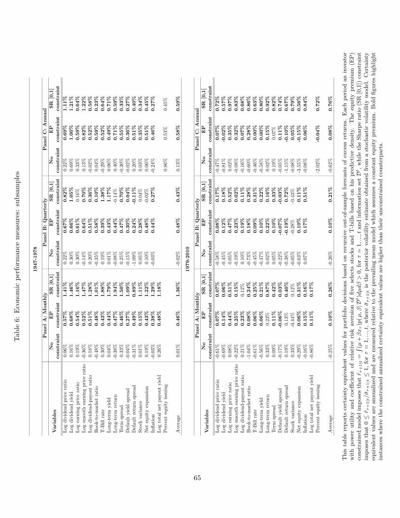
Tab

le6:

Eco

nom

icp

erfo

rman

cem

easu

res:

sub

sam

ple

s

1947-1978

PanelA:M

onth

lyPanelB:Quarterly

PanelC:Annual

Variables

No

EP

SR

[0,1]

No

EP

SR

[0,1]

No

EP

SR

[0,1]

constra

int

constra

int

constra

int

constra

int

constra

int

constra

int

constra

int

constra

int

constra

int

Log

div

iden

dp

rice

rati

o0.

06%

0.57%

1.41%

0.22

%0.67%

0.82%

0.22

%0.69%

1.11%

Log

div

iden

dyie

ld0.

16%

0.68%

1.46%

0.30

%0.66%

1.05%

0.69

%1.00%

1.21%

Log

earn

ing

pri

cera

tio

0.19

%0.54%

1.16%

0.30

%0.61%

0.16

%0.

33%

0.59%

0.64%

Log

smoot

hea

rnin

gp

rice

rati

o-0

.36%

0.52%

1.47%

-0.1

4%0.64%

0.70%

0.13

%0.82%

1.22%

Log

div

iden

d-p

ayou

tra

tio

0.18

%0.51%

1.28%

0.20

%0.51%

0.36%

-0.0

2%

0.52%

0.58%

Book

-to-

mar

ket

rati

o-0

.48%

0.48%

1.01%

-0.3

5%0.58%

0.10%

0.04

%0.59%

0.23%

T-B

ill

rate

0.30

%0.43%

1.88%

0.19

%0.39%

1.38%

-0.2

9%

0.52%

0.64%

Lon

g-te

rmyie

ld0.

04%

0.44%

1.79%

0.01

%0.43%

1.17%

0.06

%0.49%

0.71%

Lon

g-te

rmre

turn

-0.3

8%0.47%

1.94%

-0.0

8%0.44%

-0.1

4%0.

40%

0.71%

0.59%

Ter

msp

read

0.33

%0.46%

1.50%

0.25

%0.47%

0.70%

-0.3

0%

0.55%

0.33%

Def

ault

yie

ldsp

read

-0.0

4%0.27%

1.09%

-0.1

5%0.30%

0.04%

-0.0

2%

0.36%

0.27%

Def

ault

retu

rnsp

read

-0.3

1%0.49%

0.89%

-1.0

9%0.24%

-0.11%

0.20

%0.51%

0.40%

Sto

ckva

rian

ce0.

01%

0.15%

1.11%

0.05

%0.28%

0.04

%0.

03%

0.35%

0.34%

Net

equ

ity

exp

ansi

on0.

19%

0.43%

1.22%

0.10

%0.48%

-0.0

2%0.

06%

0.51%

0.45%

Infl

atio

n-0

.03%

0.38%

1.29%

-0.0

3%0.44%

0.27%

-0.2

4%

0.46%

0.27%

Log

tota

ln

etp

ayou

tyie

ld0.

26%

0.48%

1.18%

Per

cent

equ

ity

issu

ing

0.86

%0.

53%

0.4

5%

Ave

rage

0.01

%0.46%

1.36%

-0.0

2%0.48%

0.43%

0.13

%0.58%

0.59%

1979-2010

PanelA:M

onth

lyPanelB:Quarterly

PanelC:Annual

Variables

No

EP

SR

[0,1]

No

EP

SR

[0,1]

No

EP

SR

[0,1]

constra

int

constra

int

constra

int

constra

int

constra

int

constra

int

constra

int

constra

int

constra

int

Log

div

iden

dp

rice

rati

o-0

.61%

0.07%

0.07%

-0.5

8%0.08%

0.17%

-0.4

7%

0.07%

0.72%

Log

div

iden

dyie

ld-0

.69%

0.14%

0.06%

-0.4

5%0.12%

0.18%

-0.8

1%

-0.02%

0.57%

Log

earn

ing

pri

cera

tio

0.08

%0.44%

0.51%

0.05

%0.47%

0.52%

0.02

%0.35%

0.97%

Log

smoot

hea

rnin

gp

rice

rati

o-0

.22%

0.25%

0.15%

-0.1

9%0.23%

0.02%

-0.0

8%

0.32%

0.83%

Log

div

iden

d-p

ayou

tra

tio

0.21

%0.23%

0.12

%0.

10%

0.19%

0.11%

-0.1

6%

0.07%

0.68%

Book

-to-

mar

ket

rati

o-1

.04%

0.08%

0.24%

-0.7

3%0.18%

0.28%

-0.6

0%

0.28%

0.86%

T-B

ill

rate

-0.6

1%0.06%

0.25%

-0.4

5%0.09%

0.31%

-0.4

6%

0.00%

0.63%

Lon

g-te

rmyie

ld-0

.56%

0.06%

0.21%

-0.4

7%0.10%

0.22%

-0.5

8%

0.00%

0.80%

Lon

g-te

rmre

turn

0.33

%0.

23%

0.87%

0.02

%0.22%

0.16%

0.02

%0.15%

0.92%

Ter

msp

read

0.09

%0.11%

0.42%

0.05

%0.10%

0.33%

0.19

%0.

07%

0.82%

Def

ault

yie

ldsp

read

-0.1

7%-0.06%

0.03%

-0.2

2%-0.07%

-0.03%

-0.0

5%

0.11%

0.74%

Def

ault

retu

rnsp

read

0.19

%0.

13%

0.40%

-0.3

8%-0.19%

0.72%

-1.1

5%

-0.10%

0.67%

Sto

ckva

rian

ce0.

33%

-0.4

4%0.

12%

-0.0

5%-0

.28%

-0.4

3%-0

.08%

0.05%

0.79%

Net

equ

ity

exp

ansi

on-0

.29%

0.06%

0.31%

-0.6

3%0.10%

0.11%

-3.5

5%

-0.15%

0.56%

Infl

atio

n-0

.16%

0.15%

0.16%

0.07

%0.17%

0.51%

-0.0

8%

0.06%

0.84%

Log

tota

ln

etp

ayou

tyie

ld-0

.86%

0.11%

0.17%

Per

cent

equ

ity

issu

ing

-2.0

2%

-0.04%

0.72%

Ave

rage

-0.2

5%0.10%

0.26%

-0.2

6%0.10%

0.21%

-0.6

2%

0.08%

0.76%

This

table

rep

ort

sce

rtain

tyeq

uiv

ale

nt

valu

esfo

rp

ort

folio

dec

isio

ns

base

don

recu

rsiv

eout-

of-

sam

ple

fore

cast

sof

exce

ssre

turn

s.E

ach

per

iod

an

inves

tor

wit

hp

ower

uti

lity

and

coeffi

cien

tof

rela

tive

risk

aver

sion

of

five

sele

cts

stock

sand

T-b

ills

base

don

his

pre

dic

tive

den

sity

.T

he

equit

ypre

miu

m(E

P)

const

rain

edm

odel

imp

ose

sth

atr τ

+1|t

=∫ (µ

+βxτ)p

(µ,β|D

t)dµdβ>

0,

forτ

=1,...,t

and

info

rmati

on

setDt,

while

the

Sharp

era

tio

(SR

[0,1

])co

nst

rain

tim

pose

sth

at

0≤r τ

+1|t/στ+1|t≤

1,

forτ

=1,...,t

,w

her

eστ+1|t

isth

ep

ost

erio

rvola

tility

esti

mate

obta

ined

from

ast

och

ast

icvola

tility

model

.C

erta

inty

equiv

ale

nt

valu

esare

annualize

dand

are

mea

sure

dre

lati

ve

toth

epre

vailin

gm

ean

model

whic

hass

um

esa

const

ant

equit

ypre

miu

m.

Bold

figure

shig

hlight

inst

ance

sw

her

eth

eco

nst

rain

edannualize

dce

rtain

tyeq

uiv

ale

nt

valu

esare

hig

her

than

thei

runco

nst

rain

edco

unte

rpart

s.

65

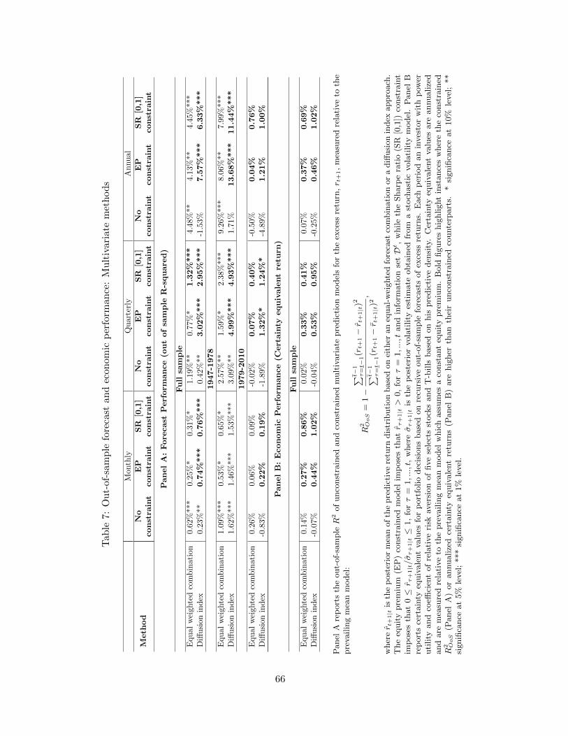
Tab

le7:

Ou

t-of

-sam

ple

fore

cast

and

econ

omic

per

form

ance

:M

ult

ivar

iate

met

hod

s

Mon

thly

Qu

arte

rly

An

nu

al

Meth

od

No

EP

SR

[0,1]

No

EP

SR

[0,1]

No

EP

SR

[0,1]

constra

int

constra

int

constra

int

constra

int

constra

int

constra

int

constra

int

constra

int

constra

int

PanelA:Fore

cast

Perform

ance(o

utofsa

mple

R-square

d)

Full

sample

Equ

alw

eigh

ted

com

bin

atio

n0.

62%

***

0.25

%*

0.31

%*

1.1

9%**

0.77

%*

1.32%***

4.48

%**

4.1

3%**

4.45

%***

Diff

usi

onin

dex

0.23

%**

0.74%***

0.76%***

0.4

2%**

3.02%***

2.95%***

-1.5

3%

7.57%***

6.33%***

1947-1978

Equ

alw

eigh

ted

com

bin

atio

n1.

09%

***

0.53

%*

0.65

%*

2.5

7%**

1.59

%*

2.38

%***

9.26

%***

8.0

6%**

7.99

%***

Diff

usi

onin

dex

1.62

%**

*1.

46%

***

1.53

%**

*3.0

9%**

4.99%***

4.93%***

1.71

%13.68%***

11.44%***

1979-2010

Equ

alw

eigh

ted

com

bin

atio

n0.

26%

0.06

%0.

09%

-0.0

2%0.07%

0.40%

-0.5

0%

0.04%

0.76%

Diff

usi

onin

dex

-0.8

3%0.22%

0.19%

-1.8

9%1.32%*

1.24%*

-4.8

9%

1.21%

1.00%

PanelB:Economic

Perform

ance(C

ertainty

equivalentre

turn

)

Full

sample

Equ

alw

eigh

ted

com

bin

atio

n0.

14%

0.27%

0.86%

0.0

2%0.33%

0.41%

0.07

%0.37%

0.69%

Diff

usi

onin

dex

-0.0

7%0.44%

1.02%

-0.0

4%0.53%

0.95%

-0.2

5%

0.46%

1.02%

Panel

Are

port

sth

eout-

of-

sam

pleR

2of

unco

nst

rain

edand

const

rain

edm

ult

ivari

ate

pre

dic

tion

model

sfo

rth

eex

cess

retu

rn,r t

+1,

mea

sure

dre

lati

ve

toth

epre

vailin

gm

ean

model

:

R2 OoS

=1−

∑ t−1

τ=t−

1(rt+

1−r t

+1|t

)2

∑ t−1

τ=t−

1(rt+

1−r t

+1|t

)2,

wher

er t

+1|t

isth

ep

ost

erio

rm

ean

of

the

pre

dic

tive

retu

rndis

trib

uti

on

base

don

eith

eran

equal-

wei

ghte

dfo

reca

stco

mbin

ati

on

or

adiff

usi

on

index

appro

ach

.T

he

equit

ypre

miu

m(E

P)

const

rain

edm

odel

imp

ose

sth

atr τ

+1|t>

0,

forτ

=1,...,t

and

info

rmati

on

setDt,

while

the

Sharp

era

tio

(SR

[0,1

])co

nst

rain

tim

pose

sth

at

0≤r τ

+1|t/στ+1|t≤

1,

forτ

=1,...,t

,w

her

eστ+1|t

isth

ep

ost

erio

rvola

tility

esti

mate

obta

ined

from

ast

och

ast

icvola

tility

model

.P

anel

Bre

port

sce

rtain

tyeq

uiv

ale

nt

valu

esfo

rp

ort

folio

dec

isio

ns

base

don

recu

rsiv

eout-

of-

sam

ple

fore

cast

sof

exce

ssre

turn

s.E

ach

per

iod

an

inves

tor

wit

hp

ower

uti

lity

and

coeffi

cien

tof

rela

tive

risk

aver

sion

of

five

sele

cts

stock

sand

T-b

ills

base

don

his

pre

dic

tive

den

sity

.C

erta

inty

equiv

ale

nt

valu

esare

annualize

dand

are

mea

sure

dre

lati

ve

toth

epre

vailin

gm

ean

model

whic

hass

um

esa

const

ant

equit

ypre

miu

m.

Bold

figure

shig

hlight

inst

ance

sw

her

eth

eco

nst

rain

edR

2 OoS

(Panel

A)

or

annualize

dce

rtain

tyeq

uiv

ale

nt

retu

rns

(Panel

B)

are

hig

her

than

thei

runco

nst

rain

edco

unte

rpart

s.*

signifi

cance

at

10%

level

;**

signifi

cance

at

5%

level

;***

signifi

cance

at

1%

level

.

66

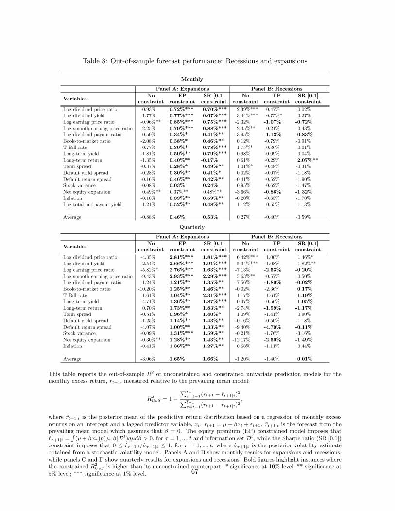
Table 8: Out-of-sample forecast performance: Recessions and expansions

Monthly

Panel A: Expansions Panel B: Recessions

VariablesNo EP SR [0,1] No EP SR [0,1]

constraint constraint constraint constraint constraint constraint

Log dividend price ratio -0.93% 0.72%*** 0.70%*** 2.39%*** 0.47% 0.02%Log dividend yield -1.77% 0.77%*** 0.67%*** 3.44%*** 0.75%* 0.27%Log earning price ratio -0.96%** 0.85%*** 0.75%*** -2.32% -1.07% -0.72%Log smooth earning price ratio -2.25% 0.79%*** 0.88%*** 2.45%** -0.21% -0.43%Log dividend-payout ratio -0.50% 0.34%* 0.41%** -3.95% -1.13% -0.83%Book-to-market ratio -2.08% 0.38%* 0.46%** 0.12% -0.79% -0.91%T-Bill rate -0.77% 0.30%* 0.78%*** 1.75%* -0.36% -0.01%Long-term yield -1.81% 0.50%** 0.79%*** 0.98% -0.09% 0.04%Long-term return -1.35% 0.40%** -0.17% 0.61% -0.29% 2.07%**Term spread -0.37% 0.28%* 0.49%** 1.01%* -0.48% -0.31%Default yield spread -0.28% 0.30%** 0.41%* 0.02% -0.07% -1.18%Default return spread -0.16% 0.46%** 0.42%** -0.41% -0.52% -1.90%Stock variance -0.08% 0.03% 0.24% 0.95% -0.62% -1.47%Net equity expansion 0.49%** 0.37%** 0.48%** -3.66% -0.86% -1.32%Inflation -0.10% 0.39%** 0.59%** -0.20% -0.63% -1.70%Log total net payout yield -1.21% 0.52%** 0.48%** 1.12% -0.55% -1.13%

Average -0.88% 0.46% 0.53% 0.27% -0.40% -0.59%

Quarterly

Panel A: Expansions Panel B: Recessions

VariablesNo EP SR [0,1] No EP SR [0,1]

constraint constraint constraint constraint constraint constraint

Log dividend price ratio -4.35% 2.81%*** 1.81%*** 6.42%*** 1.00% 1.46%*Log dividend yield -2.54% 2.66%*** 1.91%*** 5.94%*** 1.08% 1.82%**Log earning price ratio -5.82%* 2.76%*** 1.63%*** -7.13% -2.53% -0.20%Log smooth earning price ratio -9.43% 2.93%*** 2.29%*** 5.63%** -0.57% 0.50%Log dividend-payout ratio -1.24% 1.21%** 1.35%** -7.56% -1.80% -0.02%Book-to-market ratio -10.20% 1.25%** 1.46%** -0.02% -2.36% 0.17%T-Bill rate -1.61% 1.04%** 2.31%*** 1.17% -1.61% 1.19%Long-term yield -4.71% 1.36%** 1.87%*** 0.47% -0.56% 1.05%Long-term return 0.70% 1.73%** 1.83%** -2.74% -1.59% -1.17%Term spread -0.51% 0.96%* 1.40%* 1.09% -1.41% 0.90%Default yield spread -1.25% 1.14%** 1.43%** -0.16% -0.50% -1.18%Default return spread -4.07% 1.00%** 1.33%** -9.40% -4.70% -0.11%Stock variance -0.09% 1.31%*** 1.59%** -0.21% -1.76% -3.16%Net equity expansion -0.30%** 1.28%** 1.43%** -12.17% -2.50% -1.49%Inflation -0.41% 1.36%** 1.27%** 0.68% -1.11% 0.44%

Average -3.06% 1.65% 1.66% -1.20% -1.40% 0.01%

This table reports the out-of-sample R2 of unconstrained and constrained univariate prediction models for themonthly excess return, rt+1, measured relative to the prevailing mean model:

R2OoS = 1−

∑t−1τ=t−1(rt+1 − rt+1|t)

2∑t−1τ=t−1(rt+1 − rt+1|t)2

,

where rt+1|t is the posterior mean of the predictive return distribution based on a regression of monthly excessreturns on an intercept and a lagged predictor variable, xt: rt+1 = µ+ βxt + εt+1. rt+1|t is the forecast from theprevailing mean model which assumes that β = 0. The equity premium (EP) constrained model imposes thatrτ+1|t =

∫(µ+ βxτ )p(µ, β| Dt)dµdβ > 0, for τ = 1, ..., t and information set Dt, while the Sharpe ratio (SR [0,1])

constraint imposes that 0 ≤ rτ+1|t/στ+1|t ≤ 1, for τ = 1, ..., t, where στ+1|t is the posterior volatility estimateobtained from a stochastic volatility model. Panels A and B show monthly results for expansions and recessions,while panels C and D show quarterly results for expansions and recessions. Bold figures highlight instances wherethe constrained R2

OoS is higher than its unconstrained counterpart. * significance at 10% level; ** significance at5% level; *** significance at 1% level. 67

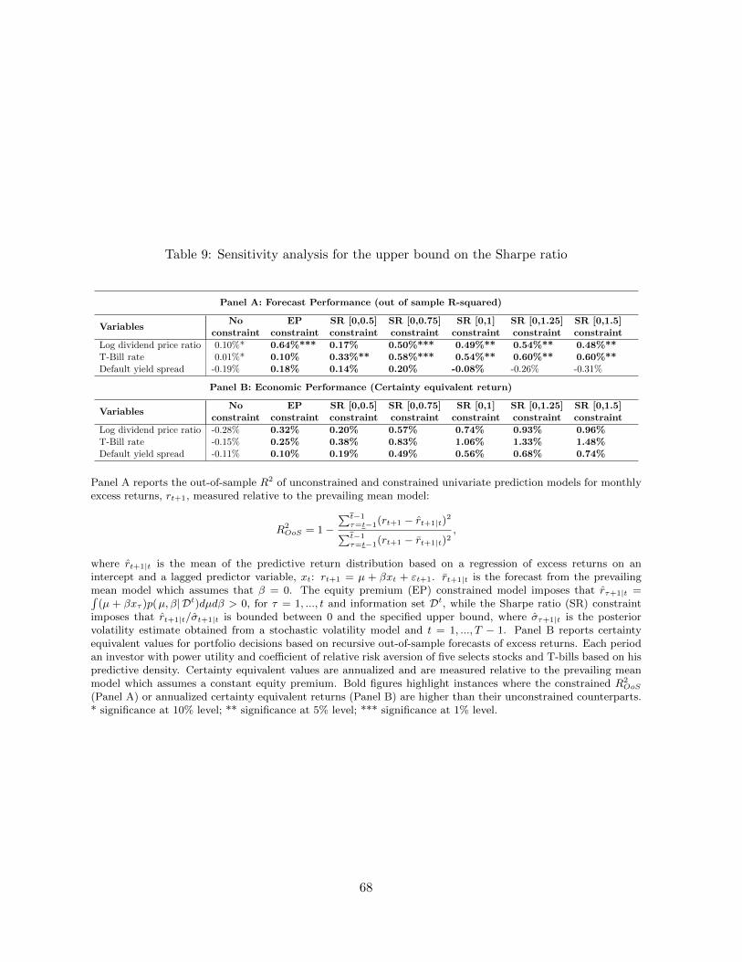
Table 9: Sensitivity analysis for the upper bound on the Sharpe ratio

Panel A: Forecast Performance (out of sample R-squared)

VariablesNo EP SR [0,0.5] SR [0,0.75] SR [0,1] SR [0,1.25] SR [0,1.5]

constraint constraint constraint constraint constraint constraint constraint

Log dividend price ratio 0.10%* 0.64%*** 0.17% 0.50%*** 0.49%** 0.54%** 0.48%**T-Bill rate 0.01%* 0.10% 0.33%** 0.58%*** 0.54%** 0.60%** 0.60%**Default yield spread -0.19% 0.18% 0.14% 0.20% -0.08% -0.26% -0.31%

Panel B: Economic Performance (Certainty equivalent return)

VariablesNo EP SR [0,0.5] SR [0,0.75] SR [0,1] SR [0,1.25] SR [0,1.5]

constraint constraint constraint constraint constraint constraint constraint

Log dividend price ratio -0.28% 0.32% 0.20% 0.57% 0.74% 0.93% 0.96%T-Bill rate -0.15% 0.25% 0.38% 0.83% 1.06% 1.33% 1.48%Default yield spread -0.11% 0.10% 0.19% 0.49% 0.56% 0.68% 0.74%

Panel A reports the out-of-sample R2 of unconstrained and constrained univariate prediction models for monthlyexcess returns, rt+1, measured relative to the prevailing mean model:

R2OoS = 1−

∑t−1τ=t−1(rt+1 − rt+1|t)

2∑t−1τ=t−1(rt+1 − rt+1|t)2

,

where rt+1|t is the mean of the predictive return distribution based on a regression of excess returns on anintercept and a lagged predictor variable, xt: rt+1 = µ + βxt + εt+1. rt+1|t is the forecast from the prevailingmean model which assumes that β = 0. The equity premium (EP) constrained model imposes that rτ+1|t =∫

(µ + βxτ )p(µ, β| Dt)dµdβ > 0, for τ = 1, ..., t and information set Dt, while the Sharpe ratio (SR) constraintimposes that rt+1|t/σt+1|t is bounded between 0 and the specified upper bound, where στ+1|t is the posteriorvolatility estimate obtained from a stochastic volatility model and t = 1, ..., T − 1. Panel B reports certaintyequivalent values for portfolio decisions based on recursive out-of-sample forecasts of excess returns. Each periodan investor with power utility and coefficient of relative risk aversion of five selects stocks and T-bills based on hispredictive density. Certainty equivalent values are annualized and are measured relative to the prevailing meanmodel which assumes a constant equity premium. Bold figures highlight instances where the constrained R2

OoS

(Panel A) or annualized certainty equivalent returns (Panel B) are higher than their unconstrained counterparts.* significance at 10% level; ** significance at 5% level; *** significance at 1% level.

68

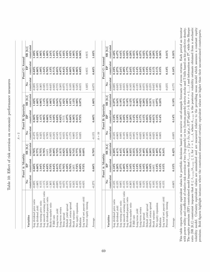
Tab

le10:

Eff

ect

ofri

skav

ersi

onon

econ

omic

per

form

ance

mea

sure

s

A=

2

PanelA:M

onth

lyPanelB:Quarterly

PanelC:Annual

Variables

No

EP

SR

[0,1]

No

EP

SR

[0,1]

No

EP

SR

[0,1]

constra

int

constra

int

constra

int

constra

int

constra

int

constra

int

constra

int

constra

int

constra

int

Log

div

iden

dp

rice

rati

o-0

.89%

0.68%

0.78%

-0.4

7%0.90%

1.02%

-0.2

0%

0.83%

1.09%

Log

div

iden

dyie

ld-1

.06%

0.66%

0.77%

-0.2

2%0.92%

1.00%

-0.5

1%

0.90%

1.09%

Log

earn

ing

pri

cera

tio

0.15

%1.04%

0.75%

0.32

%1.41%

0.96%

0.36

%1.09%

1.06%

Log

smoot

hea

rnin

gp

rice

rati

o-1

.11%

0.72%

0.78%

-0.8

5%0.96%

1.14%

-0.3

3%

1.04%

1.08%

Log

div

iden

d-p

ayou

tra

tio

0.70

%0.83%

0.64

%0.

79%

0.86%

0.93%

0.15

%0.76%

1.00%

Book

-to-

mar

ket

rati

o-1

.36%

0.73%

0.73%

-1.0

5%1.13%

1.06%

-0.6

4%

1.13%

1.24%

T-B

ill

rate

-0.2

9%0.64%

0.89%

-0.2

4%0.59%

1.03%

-0.9

2%

0.71%

1.01%

Lon

g-te

rmyie

ld-0

.69%

0.61%

0.72%

-0.5

4%0.63%

0.94%

-0.7

1%

0.65%

1.02%

Lon

g-te

rmre

turn

-0.1

2%0.77%

1.31%

-0.1

1%0.82%

0.67%

0.38

%0.87%

1.07%

Ter

msp

read

0.67

%0.76%

0.82%

0.85

%0.

71%

1.02%

-0.0

7%

0.84%

1.03%

Def

ault

yie

ldsp

read

-0.1

7%0.33%

0.83%

-0.3

7%0.37%

1.08%

-0.1

1%

0.53%

1.02%

Def

ault

retu

rnsp

read

0.01

%0.76%

0.83%

-1.1

7%0.68%

1.01%

0.10

%0.80%

1.02%

Sto

ckva

rian

ce0.

34%

0.26

%0.74%

0.00

%0.36%

1.13%

-0.0

9%

0.48%

1.00%

Net

equ

ity

exp

ansi

on0.

45%

0.72%

0.77%

0.71

%0.91%

0.99%

0.52

%0.96%

0.93%

Infl

atio

n-0

.12%

0.69%

0.59%

0.03

%0.73%

0.97%

-0.0

1%

0.83%

0.98%

Log

tota

ln

etp

ayou

tyie

ld-0

.83%

0.73%

0.69%

Per

cent

equ

ity

issu

ing

1.02

%0.8

5%

0.9

1%

Ave

rage

-0.2

7%0.68%

0.79%

-0.1

5%0.80%

1.00%

-0.0

7%

0.83%

1.03%

A=

10

PanelA:M

onth

lyPanelB:Quarterly

PanelC:Annual

Variables

No

EP

SR

[0,1]

No

EP

SR

[0,1]

No

EP

SR

[0,1]

constra

int

constra

int

constra

int

constra

int

constra

int

constra

int

constra

int

constra

int

constra

int

Log

div

iden

dp

rice

rati

o-0

.13%

0.18%

0.39%

-0.1

0%0.19%

0.27%

-0.0

9%

0.19%

0.49%

Log

div

iden

dyie

ld-0

.13%

0.20%

0.41%

-0.0

6%0.19%

0.34%

-0.0

4%

0.27%

0.47%

Log

earn

ing

pri

cera

tio

0.08

%0.27%

0.44%

0.09

%0.26%

0.19%

0.04

%0.24%

0.44%

Log

smoot

hea

rnin

gp

rice

rati

o-0

.15%

0.20%

0.43%

-0.1

0%0.23%

0.21%

-0.0

5%

0.29%

0.55%

Log

div

iden

d-p

ayou

tra

tio

0.12

%0.19%

0.36%

0.09

%0.18%

0.16%

-0.0

3%

0.17%

0.32%

Book

-to-

mar

ket

rati

o-0

.36%

0.16%

0.33%

-0.2

5%0.20%

0.12%

-0.1

6%

0.24%

0.29%

T-B

ill

rate

-0.0

8%0.13%

0.55%

-0.0

8%0.12%

0.44%

-0.2

0%

0.15%

0.35%

Lon

g-te

rmyie

ld-0

.13%

0.13%

0.52%

-0.1

4%0.13%

0.36%

-0.1

3%

0.14%

0.40%

Lon

g-te

rmre

turn

0.00

%0.19%

0.74%

-0.0

3%0.17%

-0.02%

0.08

%0.24%

0.37%

Ter

msp

read

0.12

%0.16%

0.49%

0.06

%0.15%

0.29%

-0.0

7%

0.18%

0.32%

Def

ault

yie

ldsp

read

-0.0

4%0.06%

0.29%

-0.1

0%0.05%

0.03%

-0.0

2%

0.13%

0.27%

Def

ault

retu

rnsp

read

-0.0

7%0.16%

0.28%

-0.3

8%0.02%

0.21%

-0.2

5%

0.12%

0.28%

Sto

ckva

rian

ce0.

10%

-0.0

8%0.33%

-0.0

2%-0.01%

-0.0

9%-0

.04%

0.11%

0.29%

Net

equ

ity

exp

ansi

on-0

.12%

0.13%

0.40%

-0.3

6%0.15%

0.07%

-1.4

9%

0.11%

0.24%

Infl

atio

n-0

.04%

0.13%

0.37%

0.00

%0.14%

0.23%

-0.0

9%

0.15%

0.26%

Log

tota

ln

etp

ayou

tyie

ld-0

.15%

0.15%

0.34%

Per

cent

equ

ity

issu

ing

-0.2

5%

0.13%

0.31%

Ave

rage

-0.0

6%0.15%

0.42%

-0.0

9%0.14%

0.19%

-0.1

7%

0.18%

0.35%

This

table

rep

ort

sce

rtain

tyeq

uiv

ale

nt

valu

esfo

rp

ort

folio

dec

isio

ns

base

don

recu

rsiv

eout-

of-

sam

ple

fore

cast

sof

exce

ssre

turn

s.E

ach

per

iod

an

inves

tor

wit

hp

ower

uti

lity

and

coeffi

cien

tof

rela

tive

risk

aver

sion

of

two

(top

panel

s)or

ten

(bott

om

panel

s)se

lect

sst

ock

sand

T-b

ills

base

don

his

pre

dic

tive

den

sity

.T

he

equit

ypre

miu

m(E

P)

const

rain

edm

odel

imp

ose

sth

atr τ

+1|t

=∫ (µ

+βxτ)p

(µ,β|D

t)dµdβ>

0,

forτ

=1,...,t

and

info

rmati

on

setDt,

while

the

Sharp

era

tio

(SR

[0,1

])co

nst

rain

tim

pose

sth

at

0≤r τ

+1|t/στ+1|t≤

1,

forτ

=1,...,t

,w

her

eστ+1|t

isth

ep

ost

erio

rvola

tility

esti

mate

obta

ined

from

ast

och

ast

icvola

tility

model

.C

erta

inty

equiv

ale

nt

valu

esare

annualize

dand

are

mea

sure

dre

lati

ve

toth

epre

vailin

gm

ean

model

whic

hass

um

esa

const

ant

equit

ypre

miu

m.

Bold

figure

shig

hlight

inst

ance

sw

her

eth

eco

nst

rain

edannualize

dce

rtain

tyeq

uiv

ale

nt

valu

esare

hig

her

than

thei

runco

nst

rain

edco

unte

rpart

s.

69

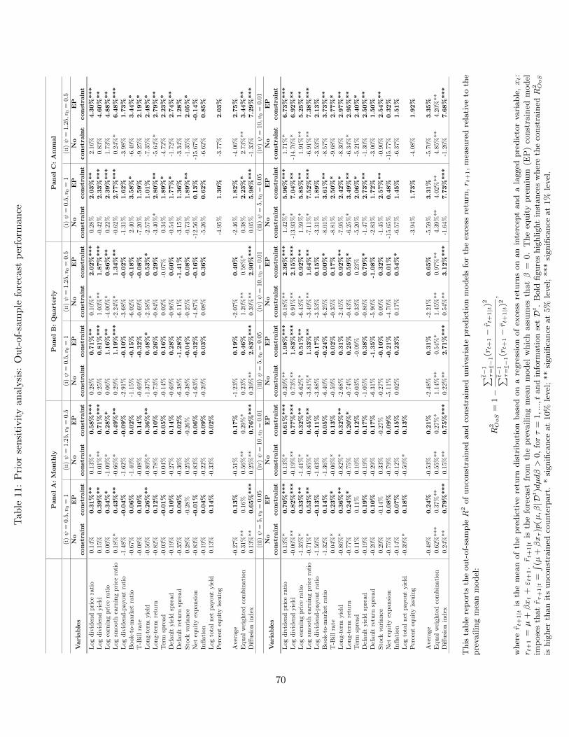
Tab

le11

:P

rior

sen

siti

vit

yan

alysi

s:O

ut-

of-s

amp

lefo

reca

stp

erfo

rman

ce

PanelA:M

onth

lyPanelB:Quarterly

PanelC:Annual

(i)ψ

=0.

5,v

0=

1(i

i)ψ

=1.

25,v

0=

0.5

(i)ψ

=0.

5,v 0

=1

(ii)ψ

=1.

25,v

0=

0.5

(i)ψ

=0.

5,v 0

=1

(ii)ψ

=1.

25,v 0

=0.

5

Variables

No

EP

No

EP

No

EP

No

EP

No

EP

No

EP

constra

int

constra

int

constra

int

constra

int

constra

int

constra

int

constra

int

constra

int

constra

int

constra

int

constra

int

constra

int

Log

div

iden

dpri

cera

tio

0.14%

0.31%**

0.13

%*

0.58%***

0.28

%0.71%**

0.10

%*

2.02%***

0.28%

2.03%**

2.1

6%

4.30%***

Log

div

iden

dyie

ld0.

15%

0.39%**

0.01

%**

0.71%***

0.25

%0.81%***

1.03

%**

1.87%***

-0.4

2%

2.33%***

0.8

3%

4.60%**

Log

earn

ing

pri

cera

tio

0.06%

0.34%*

-1.0

9%*

0.28%*

0.06

%1.16%**

-4.0

0%*

0.86%**

0.22%

2.39%***

1.7

3%

4.88%**

Log

smoot

hea

rnin

gp

rice

rati

o0.

18%

*0.43%**

-0.6

6%*

0.49%**

0.29

%1.19%***

-2.2

4%*

1.34%**

-0.6

2%

2.77%***

0.2

4%

*6.48%***

Log

div

iden

d-p

ayou

tra

tio

-1.4

8%-0.04%

-1.6

2%-0.09%

-2.9

1%-0.10%

-3.6

8%-0.02%

-1.3

1%

1.62%

-3.9

8%

1.73%

Book-t

o-m

arke

tra

tio

-0.6

7%0.06%

-1.4

0%0.02%

-1.1

5%-0.15%

-6.0

2%-0.18%

2.40%

3.58%*

-6.4

9%

3.44%*

T-B

ill

rate

-0.0

8%0.10%

-0.0

8%0.14%

-0.6

9%-0.32%

-0.6

9%-0.08%

-7.2

0%

1.59%

-9.2

5%

2.19%*

Lon

g-te

rmyie

ld-0

.56%

0.26%**

-0.8

9%*

0.36%**

-1.3

7%0.48%*

-2.5

8%0.53%*

-2.5

7%

1.01%

-7.3

5%

2.48%*

Lon

g-te

rmre

turn

-0.8

2%0.12%

-0.7

8%0.10%

-0.7

3%0.26%

-0.8

4%0.29%

-3.4

0%

*2.80%**

-5.6

4%

*2.79%**

Ter

msp

read

-0.0

3%-0.01%

0.04

%0.05%

-0.1

4%0.16%

0.02

%-0

.07%

0.34%

1.89%*

-4.7

2%

2.23%*

Def

ault

yie

ldsp

read

-0.1

9%0.10%

-0.2

7%0.14%

-0.6

9%0.28%

-0.9

6%0.60%

-0.5

4%

1.77%*

-1.7

2%

2.74%**

Def

ault

retu

rnsp

read

-0.3

5%0.06%

-0.3

6%0.02%

-6.3

8%-1.28%

-6.1

1%-1.41%

-3.1

5%

1.36%

-3.3

4%

1.28%

Sto

ckva

rian

ce0.

28%

-0.2

8%0.

25%

-0.2

6%-0

.38%

-0.04%

-0.2

5%0.08%

-0.7

3%

1.89%**

-1.3

5%

2.05%*

Net

equ

ity

exp

an

sion

-0.8

3%-0.01%

-0.8

3%0.06%

-4.6

3%-0.32%

-4.8

7%-0.16%

-12.5

6%0.13%

-15.6

7%

-0.14%

Infl

ati

on-0

.19%

0.04%

-0.2

2%0.09%

-0.2

0%0.03%

0.08

%0.36%

-5.2

6%

0.62%

-6.6

2%

0.85%

Log

tota

ln

etp

ayou

tyie

ld0.

13%

0.14%

-0.3

3%0.02%

Per

cent

equ

ity

issu

ing

-4.9

5%

1.30%

-3.7

7%

2.03%

Ave

rage

-0.2

7%0.13%

-0.5

1%0.17%

-1.2

3%0.19%

-2.0

7%0.40%

-2.4

6%

1.82%

-4.0

6%

2.75%

Equ

alw

eigh

ted

com

bin

atio

n0.

31%

**

0.1

6%0.

56%

**0.

29%

*0.

23%

0.46%

1.20

%**

0.58

%*

0.38%

2.23%*

2.7

3%

**3.44%**

Diff

usi

on

ind

ex0.

13%

**

0.65%***

0.25

%**

0.76%***

0.39

%**

2.83%***

0.39

%**

2.90%***

0.05%

5.98%***

-1.3

3%

7.29%***

(iii

)ψ

=5,v 0

=0.

05(i

v)ψ

=10,v

0=

0.01

(iii

)ψ

=5,v 0

=0.

05(i

v)ψ

=10,v

0=

0.01

(iii

)ψ

=5,v 0

=0.

05

(iv)ψ

=10,v 0

=0.

01

Variables

No

EP

No

EP

No

EP

No

EP

No

EP

No

EP

constra

int

constra

int

constra

int

constra

int

constra

int

constra

int

constra

int

constra

int

constra

int

constra

int

constra

int

constra

int

Log

div

iden

dpri

cera

tio

0.13%

*0.70%***

0.13

%*

0.61%***

-0.3

9%**

1.98%***

-0.1

8%**

2.36%***

1.42%

*5.96%***

1.7

1%

*6.73%***

Log

div

iden

dyie

ld-0

.06%

**

0.82%***

-0.1

9%**

0.77%***

0.73

%**

1.83%***

0.91

%**

2.15%***

-13.9

3%*

7.04%**

-14.7

6%

*6.92%**

Log

earn

ing

pri

cera

tio

-1.3

5%*

0.33%**

-1.4

1%*

0.32%**

-6.6

2%*

0.51%**

-6.4

3%*

0.92%**

1.59%

*5.85%**

1.9

1%

**5.25%**

Log

smoot

hea

rnin

gp

rice

rati

o-0

.71%

*0.53%**

-0.8

5%*

0.45%**

-3.8

1%*

1.33%**

-3.4

9%**

1.64%**

-7.1

1%

*7.52%***

-6.9

1%

**

7.38%***

Log

div

iden

d-p

ayou

tra

tio

-1.5

6%-0.13%

-1.6

3%-0.11%

-3.8

8%-0.17%

-3.5

3%0.15%

-3.3

1%

1.89%

-3.5

3%

2.13%

Book-t

o-m

arke

tra

tio

-1.3

2%0.14%

-1.3

6%0.05%

-6.4

0%-0.24%

-6.2

5%0.00%*

-8.0

1%

3.61%**

-8.5

7%

3.73%**

T-B

ill

rate

0.04%

*0.23%*

-0.0

6%*

0.13%

-0.5

9%0.02%

-0.3

5%0.17%

-8.8

1%

2.50%*

-9.6

8%

2.77%*

Lon

g-te

rmyie

ld-0

.86%

*0.36%**

-0.8

2%*

0.32%**

-2.6

8%0.31%

-2.4

5%0.92%**

-7.9

5%

2.42%*

-8.3

0%

2.97%**

Lon

g-te

rmre

turn

-0.7

7%0.24%*

-0.7

5%0.20%*

-0.7

4%0.25%

-0.4

3%0.59%*

-6.2

5%

*3.49%**

-6.3

4%

*2.95%**

Ter

msp

read

0.11%

0.1

1%0.

10%

0.12%

-0.0

3%-0

.09%

0.33

%0.

23%

-5.2

0%

2.06%*

-5.2

1%

2.40%*

Def

ault

yie

ldsp

read

-0.1

9%0.19%

-0.1

9%0.17%

-1.0

5%0.38%

-0.8

6%0.79%*

-1.4

7%

2.73%**

-1.3

0%

2.50%**

Def

ault

retu

rnsp

read

-0.2

0%0.10%

-0.2

9%0.17%

-6.3

1%-1.35%

-5.9

0%-1.08%

-2.8

3%

1.72%

-3.0

6%

1.50%

Sto

ckva

rian

ce0.

29%

-0.1

4%0.

33%

-0.2

7%-0

.27%

-0.10%

0.09

%0.32%

-1.4

5%

2.57%**

-0.9

0%

2.54%**

Net

equ

ity

exp

an

sion

-0.7

5%0.08%

-0.7

9%0.09%

-5.1

1%-0.21%

-4.7

0%0.01%

-15.6

5%0.48%

-15.7

7%

0.32%

Infl

ati

on-0

.14%

0.07%

-0.1

2%0.15%

0.02

%0.23%

0.17

%0.54%*

-6.5

7%

1.45%

-6.3

7%

1.51%

Log

tota

ln

etp

ayou

tyie

ld-0

.39%

*0.18%

-0.5

0%*

0.13%

Per

cent

equ

ity

issu

ing

-3.9

4%

1.73%

-4.0

8%

1.92%

Ave

rage

-0.4

8%0.24%

-0.5

3%0.21%

-2.4

8%0.31%

-2.2

1%0.65%

-5.5

9%

3.31%

-5.7

0%

3.35%

Equ

alw

eigh

ted

com

bin

atio

n0.

62%

***

0.3

7%**

0.55

%**

0.27

%*

1.14

%**

0.54

%*

1.45

%**

0.97

%**

4.39%

**

4.0

2%

**

4.8

5%

**4.2

0%**

Diff

usi

onin

dex

0.24%

**

0.79%***

0.15

%**

0.75%***

0.22

%**

2.71%***

0.54

%**

3.12%***

-1.6

4%

7.73%***

-1.2

6%

7.68%***

This

table

rep

ort

sth

eout-

of-

sam

pleR

2of

unco

nst

rain

edand

const

rain

eduniv

ari

ate

pre

dic

tion

model

sfo

rth

eex

cess

retu

rn,r t

+1,

mea

sure

dre

lati

ve

toth

epre

vailin

gm

ean

model

:

R2 OoS

=1−

∑ t−1

τ=t−

1(rt+

1−r t

+1|t

)2

∑ t−1

τ=t−

1(rt+

1−r t

+1|t

)2,

wher

er t

+1|t

isth

em

ean

of

the

pre

dic

tive

retu

rndis

trib

uti

on

base

don

are

gre

ssio

nof

exce

ssre

turn

son

an

inte

rcep

tand

ala

gged

pre

dic

tor

vari

able

,xt:

r t+1

=µ

+βxt

+ε t

+1.r t

+1|t

isth

efo

reca

stfr

om

the

pre

vailin

gm

ean

model

whic

hass

um

esth

atβ

=0.

The

equit

ypre

miu

m(E

P)

const

rain

edm

odel

imp

ose

sth

atr τ

+1|t

=∫ (µ

+βxτ)p

(µ,β|D

t)dµdβ>

0,

forτ

=1,...,t

and

info

rmati

on

setDt.

Bold

figure

shig

hlight

inst

ance

sw

her

eth

eco

nst

rain

edR

2 OoS

ishig

her

than

its

unco

nst

rain

edco

unte

rpart

.*

signifi

cance

at

10%

level

;**

signifi

cance

at

5%

level

;***

signifi

cance

at

1%

level

.

70

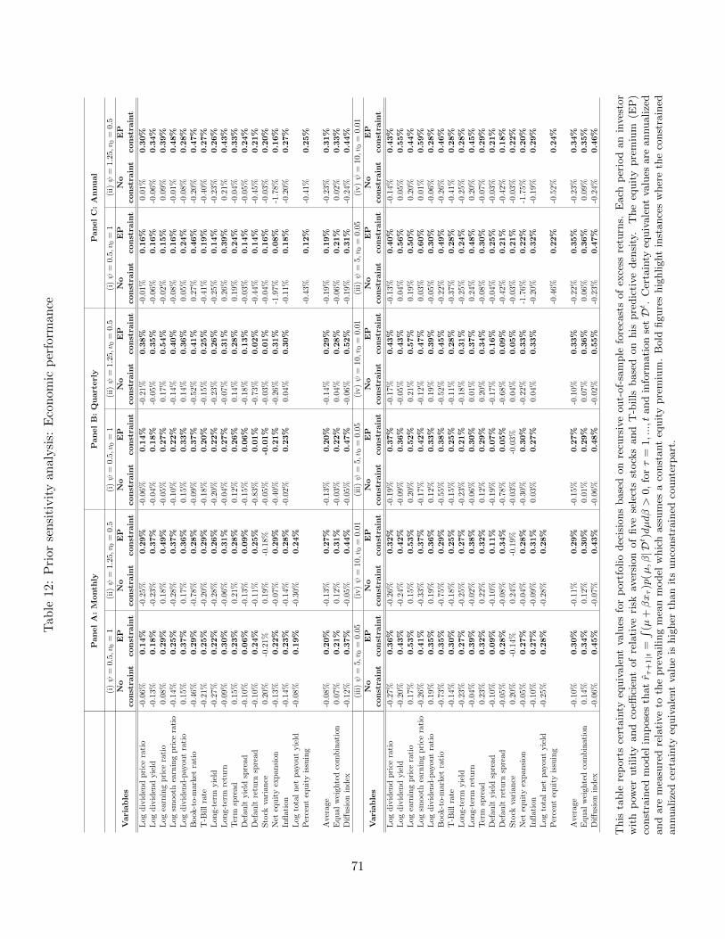
Tab

le12

:P

rior

sen

siti

vit

yan

alysi

s:E

con

omic

per

form

ance

PanelA:M

onth

lyPanelB:Quarterly

PanelC:Annual

(i)ψ

=0.

5,v

0=

1(i

i)ψ

=1.

25,v

0=

0.5

(i)ψ

=0.

5,v

0=

1(i

i)ψ

=1.

25,v

0=

0.5

(i)ψ

=0.

5,v

0=

1(i

i)ψ

=1.

25,v 0

=0.

5

Variables

No

EP

No

EP

No

EP

No

EP

No

EP

No

EP

constra

int

constra

int

constra

int

constra

int

constra

int

constra

int

constra

int

constra

int

constra

int

constra

int

constra

int

constra

int

Log

div

iden

dpri

cera

tio

-0.0

6%0.14%

-0.2

5%0.29%

-0.0

6%0.14%

-0.2

1%0.38%

-0.0

1%

0.16%

0.0

1%

0.30%

Log

div

iden

dyie

ld-0

.13%

0.18%

-0.2

3%0.37%

-0.0

4%0.18%

-0.0

5%0.35%

-0.0

6%

0.16%

-0.0

6%

0.34%

Log

earn

ing

pri

cera

tio

0.08

%0.29%

0.18

%0.49%

-0.0

5%0.27%

0.17%

0.54%

-0.0

2%

0.15%

0.0

9%

0.39%

Log

smoot

hea

rnin

gpri

cera

tio

-0.1

4%0.25%

-0.2

8%0.37%

-0.1

0%0.22%

-0.1

4%0.40%

-0.0

8%

0.16%

-0.0

1%

0.48%

Log

div

iden

d-p

ayou

tra

tio

0.15

%0.37%

0.17

%0.36%

0.15

%0.33%

0.14%

0.36%

0.0

5%

0.24%

-0.0

8%

0.28%

Book

-to-

mar

ket

rati

o-0

.46%

0.29%

-0.7

8%0.28%

-0.0

9%0.37%

-0.5

2%0.41%

0.2

7%

0.46%

-0.2

0%

0.47%

T-B

ill

rate

-0.2

1%0.25%

-0.2

0%0.29%

-0.1

8%0.20%

-0.1

5%0.25%

-0.4

1%

0.19%

-0.4

0%

0.27%

Lon

g-te

rmyie

ld-0

.27%

0.22%

-0.2

8%0.26%

-0.2

0%0.22%

-0.2

3%0.26%

-0.2

5%

0.14%

-0.2

3%

0.26%

Lon

g-te

rmre

turn

-0.0

9%0.30%

-0.0

6%0.31%

-0.0

4%0.27%

-0.0

7%0.31%

0.2

6%

0.39%

0.2

1%

0.43%

Ter

msp

read

0.15

%0.23%

0.21

%0.28%

0.12

%0.26%

0.14%

0.28%

0.1

9%

0.24%

-0.0

4%

0.33%

Def

ault

yie

ldsp

read

-0.1

0%0.06%

-0.1

3%0.09%

-0.1

5%0.06%

-0.1

8%0.13%

-0.0

3%

0.14%

-0.0

5%

0.24%

Def

ault

retu

rnsp

read

-0.1

0%0.24%

-0.1

1%0.25%

-0.8

3%0.01%

-0.7

3%0.02%

-0.4

4%

0.14%

-0.4

5%

0.21%

Sto

ckva

rian

ce0.

20%

-0.2

1%0.

19%

-0.1

8%-0

.05%

-0.01%

-0.0

3%0.01%

-0.0

4%

0.16%

-0.0

3%

0.20%

Net

equ

ity

exp

ansi

on-0

.13%

0.22%

-0.0

7%0.29%

-0.4

0%0.21%

-0.2

6%0.31%

-1.9

7%

0.08%

-1.7

8%

0.16%

Infl

atio

n-0

.14%

0.23%

-0.1

4%0.28%

-0.0

2%0.23%

0.04%

0.30%

-0.1

1%

0.18%

-0.2

0%

0.27%

Log

tota

ln

etp

ayou

tyie

ld-0

.08%

0.19%

-0.3

0%0.24%

Per

cent

equ

ity

issu

ing

-0.4

3%

0.12%

-0.4

1%

0.25%

Ave

rage

-0.0

8%0.20%

-0.1

3%0.27%

-0.1

3%0.20%

-0.1

4%0.29%

-0.1

9%

0.19%

-0.2

3%

0.31%

Equ

alw

eigh

ted

com

bin

atio

n0.

07%

0.21%

0.12

%0.31%

-0.0

3%0.22%

0.04%

0.28%

-0.0

6%

0.21%

0.0

2%

0.33%

Diff

usi

onin

dex

-0.1

2%0.37%

-0.0

5%0.44%

-0.0

5%0.47%

-0.0

6%0.52%

-0.1

9%

0.31%

-0.2

4%

0.44%

(iii

)ψ

=5,v 0

=0.

05(i

v)ψ

=10,v

0=

0.01

(iii)ψ

=5,v 0

=0.

05(i

v)ψ

=10,v 0

=0.

01(i

ii)ψ

=5,v 0

=0.

05

(iv)ψ

=10,v 0

=0.

01

Variables

No

EP

No

EP

No

EP

No

EP

No

EP

No

EP

constra

int

constra

int

constra

int

constra

int

constra

int

constra

int

constra

int

constra

int

constra

int

constra

int

constra

int

constra

int

Log

div

iden

dpri

cera

tio

-0.2

7%0.36%

-0.2

6%0.32%

-0.1

9%0.37%

-0.1

7%0.43%

-0.1

3%

0.40%

-0.1

4%

0.43%

Log

div

iden

dyie

ld-0

.20%

0.43%

-0.2

4%0.42%

-0.0

9%0.36%

-0.0

5%0.43%

0.0

4%

0.56%

0.0

5%

0.55%

Log

earn

ing

pri

cera

tio

0.17

%0.53%

0.15

%0.53%

0.20

%0.52%

0.21%

0.57%

0.1

9%

0.50%

0.2

0%

0.44%

Log

smoot

hea

rnin

gpri

cera

tio

-0.2

6%0.41%

-0.3

3%0.37%

-0.1

7%0.42%

-0.1

2%0.47%

0.0

3%

0.60%

0.0

1%

0.59%

Log

div

iden

d-p

ayou

tra

tio

0.19

%0.35%

0.19

%0.36%

0.12

%0.33%

0.19%

0.39%

-0.0

5%

0.30%

-0.0

6%

0.28%

Book

-to-

mar

ket

rati

o-0

.73%

0.35%

-0.7

5%0.29%

-0.5

5%0.38%

-0.5

2%0.45%

-0.2

2%

0.49%

-0.2

6%

0.46%

T-B

ill

rate

-0.1

4%0.30%

-0.1

8%0.25%

-0.1

5%0.25%

-0.1

1%0.28%

-0.3

7%

0.28%

-0.4

1%

0.28%

Lon

g-te

rmyie

ld-0

.23%

0.27%

-0.2

5%0.27%

-0.2

3%0.21%

-0.1

8%0.31%

-0.2

5%

0.24%

-0.2

5%

0.28%

Lon

g-te

rmre

turn

-0.0

4%0.39%

-0.0

2%0.38%

-0.0

6%0.30%

0.01%

0.37%

0.2

4%

0.48%

0.2

0%

0.45%

Ter

msp

read

0.23

%0.32%

0.22

%0.32%

0.12

%0.29%

0.20%

0.34%

-0.0

8%

0.30%

-0.0

7%

0.29%

Def

ault

yie

ldsp

read

-0.1

0%0.09%

-0.1

0%0.11%

-0.1

9%0.07%

-0.1

7%0.16%

-0.0

4%

0.25%

-0.0

3%

0.21%

Def

ault

retu

rnsp

read

-0.0

5%0.28%

-0.0

8%0.34%

-0.7

8%0.05%

-0.6

8%0.09%

-0.4

2%

0.21%

-0.4

2%

0.18%

Sto

ckva

rian

ce0.

20%

-0.1

4%0.

24%

-0.1

9%-0

.03%

-0.0

3%0.

04%

0.05%

-0.0

3%

0.21%

-0.0

3%

0.22%

Net

equ

ity

exp

ansi

on-0

.05%

0.27%

-0.0

4%0.28%

-0.3

0%0.30%

-0.2

2%0.33%

-1.7

6%

0.22%

-1.7

5%

0.20%

Infl

atio

n-0

.10%

0.27%

-0.0

9%0.31%

0.03

%0.27%

0.04%

0.33%

-0.2

0%

0.32%

-0.1

9%

0.29%

Log

tota

ln

etp

ayou

tyie

ld-0

.25%

0.28%

-0.2

8%0.28%

Per

cent

equ

ity

issu

ing

-0.4

6%

0.22%

-0.5

2%

0.24%

Ave

rage

-0.1

0%0.30%

-0.1

1%0.29%

-0.1

5%0.27%

-0.1

0%0.33%

-0.2

2%

0.35%

-0.2

3%

0.34%

Equ

alw

eigh

ted

com

bin

atio

n0.

14%

0.34%

0.12

%0.30%

0.01

%0.29%

0.07%

0.36%

0.0

6%

0.36%

0.0

9%

0.35%

Diff

usi

onin

dex

-0.0

6%0.45%

-0.0

7%0.43%

-0.0

6%0.48%

-0.0

2%0.55%

-0.2

3%

0.47%

-0.2

4%

0.46%

This

table

rep

ort

sce

rtain

tyeq

uiv

ale

nt

valu

esfo

rp

ort

folio

dec

isio

ns

base

don

recu

rsiv

eout-

of-

sam

ple

fore

cast

sof

exce

ssre

turn

s.E

ach

per

iod

an

inves

tor

wit

hp

ower

uti

lity

and

coeffi

cien

tof

rela

tive

risk

aver

sion

of

five

sele

cts

stock

sand

T-b

ills

base

don

his

pre

dic

tive

den

sity

.T

he

equit

ypre

miu

m(E

P)

const

rain

edm

odel

imp

ose

sth

atr τ

+1|t

=∫ (µ

+βxτ)p

(µ,β|D

t)dµdβ>

0,

forτ

=1,...,t

and

info

rmati

on

setDt.

Cer

tain

tyeq

uiv

ale

nt

valu

esare

annualize

dand

are

mea

sure

dre

lati

ve

toth

epre

vailin

gm

ean

model

whic

hass

um

esa

const

ant

equit

ypre

miu

m.

Bold

figure

shig

hlight

inst

ance

sw

her

eth

eco

nst

rain

edannualize

dce

rtain

tyeq

uiv

ale

nt

valu

eis

hig

her

than

its

unco

nst

rain

edco

unte

rpart

.

71