1

Asset Returns and EconomicGrowthDean Baker

Center for Economic and Policy Research

J. Bradford DeLongUniversity of California at Berkeley and NBER

Paul KrugmanPrinceton University and NBER

Draft 3.0

March 24, 20051

Preliminary: 8000 words

Abstract

We in America are probably facing a demographictransition—a slowdown in the rate of natural populationincrease—and possibly facing a slowdown in productivitygrowth as well. If these two factors do in fact push down therate of economic growth in the future, is it still prudent toassume that the past performance of assets is an indication offuture results? We argue “no.” Simple standard closed-economy growth models predict that growth slowdowns are

1 We would like to thank the National Science Foundation and U.C. Berkeley’sCommittee on Research for financial support. We would like to thank GuanWang and Konstantin Magin for excellent research assistance. And we wouldlike to thank Randy Cohen, Peter Diamond, Barry Eichengreen, Tom Maguire,Greg Mankiw, Peter Orszag, George Perry, Christie Romer, David Romer, MaxSawicky, and Robert Waldmann for helpful discussions.

2

likely to lower the marginal product of capital, and thus thelong-run rate of return. Moreover, if you assume that currentasset valuations represent rational expectations, simplearithmetic tells us that it is next to impossible for past rates ofreturn to continue through a forthcoming growth slowdown.Only a large shift in the distribution of income toward capitalor current account surpluses larger than those of nineteenthcentury Britain sustained for generations give promise forreconciling a slowdown in future economic growth with acontinuation of historical asset returns.

I. IntroductionProjections of rates of return on capital in general, and equity inparticular, play important roles in economic policy debates.Opinions on many policy issues substantially depend on whetherhistorical rates of return—especially the 6.5% or so average realrealized rate of return on equities—are likely to persist. We areprobably undergoing a transition from a twentieth century in whichthe American population’s rate of natural increase was high to atwenty-first century in which many suspect that fertility will be ator near zero-population-growth levels. And some (althoughdefinitely not Robert Gordon (2004)) are projecting a slowdown inproductivity growth. The Social Security Administration, forexample, sees economy-wide labor productivity growing at only1.6% per year in 2011 and thereafter. But between 1990 and 2004economy-wide productivity growth grew at 2.2% per year.

We are somewhat skeptical of forecasts of slowing populationgrowth. We cannot forecast natural increase. In most futures wecan think of, the world in 2050 or 2100 contains a great manypeople outside the U.S. whose productivity would be amplified ifthey were able to move to the U.S., and so we suspect that for atleast the next century immigration will play as large a role inAmerica’s future than it has in its past. We are somewhat skepticalof forecasts of persistent productivity slowdowns as well, for the

3

reasons set out by Gordon (2004), Oliner and Sichel (2003), andKremer (1993). Nevertheless, we believe that if such forecasts ofslowed real GDP growth come to pass, then returns to capital andparticularly returns to equity are highly likely to be significantlybelow past historical averages. In our view, the links between assetreturns and economic growth are likely to be relatively strong: thearithmetic of payout yields, investment, and capital stock growthrates; the algebra of capital accumulation and the productionfunction; and the standard analytical models economists use astheir finger exercises all suggest this.

We make our case in seven additional sections that follow thisintroduction. Section II lays out what we see as the major issues.Section III discusses how arithmetic tells us that rates of return andrates of growth are linked: starting from where we are now, wefind it arithmetically very difficult to construct scenarios in whichasset returns are at their historic average values and real GDPgrowth is markedly slowed.

Section IV discusses how the algebra of the production functionand capital accumulation suggests that rates of return and rates ofgrowth are linked. And section V analyzes the standard verysimple aggregate economists use for their finger exercises, andfinds that they too lead us to not be surprised by a positiverelationship between economic growth and asset returns.

Section VI turns to the most interesting possibility for escape. Inthe late nineteenth century slowed growth in the British economywas accompanied by no reduction in returns on British assets asBritain exported capital on a scale relative to the size of itseconomy never seen before or since (see Edelstein (1973)). Couldthe U.S. follow the same trajectory? Yes. Is it likely to? Notwithout a huge boost to national savings.

In section VII we turn to a brief analysis of the equity premium.Once one has conditioned on the level of the capital-output ratio,

4

returns on balanced portfolios in the long run depend only on thephysical return to capital and the margins charged by financialintermediaries.2 They do not depend on the equity premium and theprice of risk. But much argument and some analysis of thedilemmas of America’s social insurance system points to the largehistorical value of the equity return premium in America and seesthis as a potential source of excess returns.

Section VIII provides our conclusions. We conclude that ifeconomic growth over the next century falls as far as forecasts likethose contained in the Social Security Trustees Report (2005) areenvisioning, then it is possible but not likely that asset returns willmatch historical experience. If the stock market today issignificantly overvalued and about to come back to earth, if thedistribution of income undergoes a significant shift away fromlabor and toward capital, or if the United States massively boostsits national savings rate and runs surpluses on the relative scale ofpre-World War I Britain for more than twice as long as Britaindid—then a growth slowdown need not entail a significantreduction in asset returns. But these seem to us to be possiblescenarios, not the central tendency of the distribution of possiblefutures that is a real economic forecast.

Economic growth and asset returns are linked. Falls in growth ratesare very likely to be accompanied by declines in asset returns.These declines in asset returns that are likely to be larger if the fallin growth comes from a productivity slowdown than from apopulation growth slowdown. But we would be very surprised iffuture growth in either productivity or population were slower thanin the past and yet asset returns in the future matched those of thepast.

2 However, attitudes toward risk do affect the long-run capital-output ratio.

5

II. The IssuesProjections of rates of return on capital in general, and equity inparticular, have come to and will continue to play a major role ineconomic policy debates. The key question in such discussions iswhether historical rates of return—especially the 6.5% or soaverage real realized rate of return on equities—are likely to persistinto the future. We are probably undergoing a major demographictransition from a twentieth century in which the Americanpopulation’s rate of natural increase was high to a twenty-firstcentury in which many suspect that fertility will be at or near zero-population-growth levels, and in which the bulk of populationgrowth is likely to come from immigration. From 1958 to 2004hours worked grew at 1.6% per year as the entrance of baby-boomers—male and female—and their successors into the laborforce vastly outweighed a decline in average hours. The SocialSecurity Administration is currently projecting that hours workedwill grow at only 0.3% per year form 2015 on (SSA (2005)).

In addition, some forecasters are projecting a slowdown inproductivity growth. The Social Security Administration seeseconomy-wide labor productivity growing at only 1.6% per year in2011 and thereafter. But between 1995 and 2004, economy-widelabor productivity grew at 2.8%, between 1990 and 2004 at 2.2%,and between 1958 and 2004 economy-wide productivity grew at1.9%.3

Thus less than a decade from now the forecasters at the SocialSecurity Administration at least see a significant change: a fall of 3 An alternative breakdown would distinguish 1958-73, during which economy-wide labor productivity growth grew at 2.6%; the productivity slowdown periodof 1973-95, during which economy-wide productivity grew at 1.0%, and thepost-1995 “new economy” period, during which economy-wide productivitygrowth has been 2.8%. Clearly an enormous amount depends on whether weinterpret the 1973-95 productivity slowdown period as an anomalous freakdisturbance to the economy’s normal structure, or as just one of those things wecan expect to see every half century or so.

6

1.3 percentage points per year in the rate of growth of labor input,and a fall of between 0.3 and 1.2 percentage points, depending onwhether one takes the long 1958-2004 or the short 1995-2004baseline, in labor productivity growth. The total growth slowdownforecast to hit in a decade or less is thus in the range of 1.6-2.5annual percentage points.

What implications will this growth slowdown—if it comes topass—have for asset values and returns? One position, takenimplicitly by the Social Security Administration and explicitly byothers, is that there is no reason to expect asset returns to be lowerin the future. Economic growth, after all, is determined byproductivity growth and labor force growth in the United States.Asset returns are determined by time preference, the marginalutility of wealth as it declines over time, and attitudes toward risk.Why should these be connected?4 Thus, we here, past assetperformance is still the best guide to future returns.

We take a contrary position. Yes, safe asset returns are equal to themarginal utility of savings, stock market returns are safe assetreturns plus the cost of bearing equity risk, and the United States ispart of a world economy. Yes, economic growth is equal toproductivity growth plus labor force growth. But only in the caseof a small open economy are asset returns determinedindependently of the rate of economic growth. In a closed or in alarge open economy, they will be linked.

Perhaps an analogy will be helpful. In international trade, the tradebalance is the difference between exporters’ ability to sell abroadand home demand for imports. In international finance, the tradebalance is the difference between national saving and nationalinvestment. How can this be? Why should a change in exporters’success at marketing abroad change either national savings ornational investment? Great confusion has been caused throughout 4 Council of Economic Advisers (2005).

7

international economics over how, exactly, to think of theconnection. We believe that claims that national growth isunconnected with asset returns are a similar failure to grasp thewhole problem.

This is an especially important issue to get straight now because itaffects how one evaluates different approaches to social insurance.The relative attractiveness of pay-as-you-go versus prefundedsocial-insurance systems depends to some degree on the gapbetween the return on capital r and the rate of real economicgrowth n+g—the sum of the rate of growth of employment n andthe rate of growth of labor productivity g. The larger is the rate ofeconomic growth n+g relative to the return on capital r, the moreattractive do pay-as-you-go social-insurance systems become.When n+g approaches r, they appear to be cheap and effectiveways of increasing social welfare by passing resources down fromthe (rich and numerous) future to the (poor and relatively small)present.

The larger is r relative to n+g, the greater are the benefits ofprefunding social insurance systems. Prefunded systems can usehigh rates of return and compound interest to reduce the wedgebetween productivity and after-contribution real wages. They thussacrifice the possibility of raising social welfare by moving wealthfrom the richer far future to the near future and the present, but inreturn they gain by reducing the social insurance tax rate and thusits deadweight loss.

To the extent that the political debate over the future of socialinsurance in America is conducted in the language of rationalpolicy analysis, getting the gap between r on the one hand and n+gon the other hand right is important. Policies predicated on a falsebelief that r is much larger relative to n+g than it is will undulyburden the current and future young, and leave many disappointedwhen returns on assets turn out to be less than anticipated andprefunding leaves large unexpected holes in financing. Policies

8

predicated on a false belief that n+g is higher relative to r than it infact is pass up opportunities to lighten the overall tax burden andstill provide near-equivalent income security benefits in the longrun.

III. ArithmeticYields, Returns, and Economic GrowthBegin by considering the determinants of equity prices. And beginwith the Gordon equation:

(1)

€

P =D

re − g

Where D are the dividends paid on a stock or an index, P is thecorresponding price, re is the expected real rate of return onequities, and g is the expected permanent real growth rate ofdividends.

By choosing to begin with this equity-pricing equation, we havealready made a number of intellectual bets. By taking this r—thereturn on equities—as the variable of interest, we are implicitlyassuming that there are no significant large or interesting shifts inthe equity premium, and thus that changes in returns on equitieswill be associated with similar changes in returns on debt. We arealso assuming that the stock market knows what it is doing: thatcurrent market prices do accurately discount what are (or perhapswhat ought to be) expectations of future cash flows at what is (orperhaps what ought to be) the appropriate rate. These assumptionscould be questioned. We will relax the assumption of a stableequity premium in section VII. And we will occasionally wonderwhether the current market might be overvalued.

9

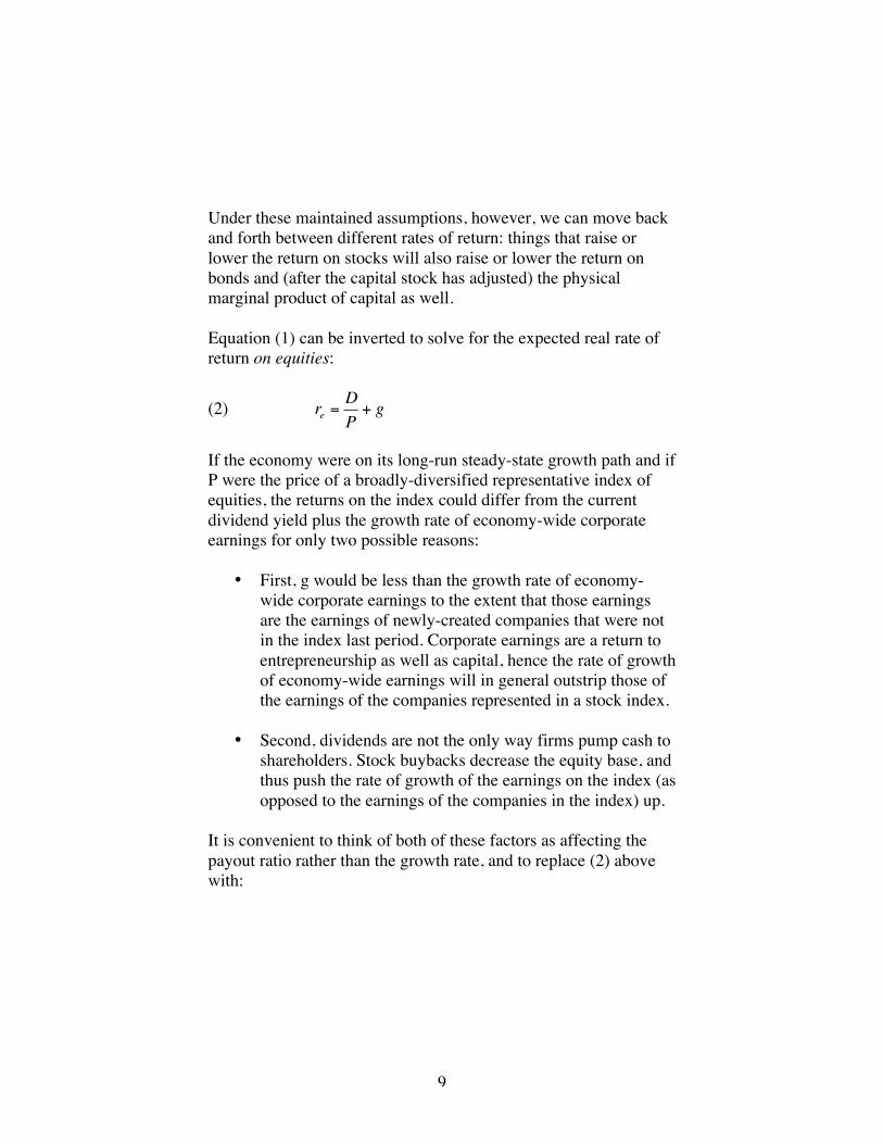
Under these maintained assumptions, however, we can move backand forth between different rates of return: things that raise orlower the return on stocks will also raise or lower the return onbonds and (after the capital stock has adjusted) the physicalmarginal product of capital as well.

Equation (1) can be inverted to solve for the expected real rate ofreturn on equities:

(2)

€

re =DP

+ g

If the economy were on its long-run steady-state growth path and ifP were the price of a broadly-diversified representative index ofequities, the returns on the index could differ from the currentdividend yield plus the growth rate of economy-wide corporateearnings for only two possible reasons:

• First, g would be less than the growth rate of economy-wide corporate earnings to the extent that those earningsare the earnings of newly-created companies that were notin the index last period. Corporate earnings are a return toentrepreneurship as well as capital, hence the rate of growthof economy-wide earnings will in general outstrip those ofthe earnings of the companies represented in a stock index.

• Second, dividends are not the only way firms pump cash toshareholders. Stock buybacks decrease the equity base, andthus push the rate of growth of the earnings on the index (asopposed to the earnings of the companies in the index) up.

It is convenient to think of both of these factors as affecting thepayout ratio rather than the growth rate, and to replace (2) abovewith:

10

(3)

€

re =D+ BP

+ g

where B are net share buybacks—buybacks less IPOs. SubtractingIPOs ensures that the ratio of total economy-wide earnings to theearnings of companies in the index does not grow. Adding grossbuybacks takes account of the anti-dilution effects of narrowingthe equity base of companies currently in the index.

Now comes the arithmetic:

Consider the 2005 Trustees Report of the Social Security System.The Report projects that 1.9 percent per year will be the averageannual rate of long-run real GDP growth measured using the GDPdeflator (Table V.B2). The Report projects that labor and capitalshares remain constant in the long-run.5 With a gap of 0.3percentage points between between the CPI and the GDP deflator(Table V.B1), and with an auxiliary assumption that capitalstructures are in balance, this is a forecast that the variable g in theGordon equation will be 1.6 percent per year.

Current dividend yields on the S&P 500 are 1.9% per year. Currentnet stock buybacks are 1.0% per year. Long-run dividend growth gis 1.6% per year. The sum of the three is 4.5% per year. That’s theexpected real rate of return r. That’s significantly lower than the6.5% real rate of return that is our historical experience with theAmerican stock market.

5 The assumption of constant income share follows from the derivation of realwage growth from productivity growth, which is discussed on pages 85-88 ofthe Trustees’ Report.

11

Possible Ways OutAre there ways to escape from this arithmetic? Yes. The U.S.economy is not on a steady state growth path. Three potential waysout seem most worth exploring:

• Perhaps the distribution of world investment will shift in away allowing U.S. companies to earn greater and greatershares of their profits abroad.

• Perhaps the stock market is currently overvalued, and willdecline and so significantly raise payout yields.

• Perhaps payout growth will be unusually rapid in the nearterm before slowing to its long-term forecast trend rate of1.6% per year.

Defer the first possibility—which we regard as the mostinteresting—to the “open economy” section later on in the paper,noting here only unless the U.S. runs a current-account surplus inthe long run corporate earnings earmarked for U.S. residents in factgrow more slowly than U.S. real GDP.

The second possibility has been advocated by Peter Diamond(2000). The arithmetic does rely on the stock market knowing whatit is doing: that there are no large windfall profits or losses outthere to be reaped by those who have better, more rationalexpectations than the marginal trader. A decline in the stockmarket relative to the economy’s growth trend of 40% would carrypayout yields up to the 4.9% consistent with a long-run real returnof 6.5% per year and real profit and dividend growth (on a CPIbasis) of 1.6% per year. With an average CPI inflation rate of 2.5%and real profit and dividend growth of 1.6% per year, such a 40%decline relative to trend would require thirteen years of nominalstagnation in equity prices. Such a scenario is certainly possible: itwas the stock market’s experience between the late 1960s and the

12

early 1980s. But we have a hard time seeing at as the centraltendency of the distribution of possible futures.6

The third possibility requires what seems to us at least to beanother unlikely scenario. If payouts—both dividends and netstock buybacks—were to grow rapidly over the next decade inorder to validate a subsequent real growth rate of 1.6% per yearand a current expected real return of 6.5% per year, the realpayouts of the companies in the index would have to grow at anaverage of 8.6% per year. Over the past fifty years, the earnings onthe S&P 500 have grown at an average rate of 2.1% per year. Onceagain, it could happen: perhaps we are in the middle of apermanent shift in the distribution of income away from labor andtoward capital that would allow equity payouts to permanentlydouble as a share of GDP over the next decade. But once again weregard this as a possible scenario, not as the central tendency of thedistribution of possible futures.

Our view that such a boom in payouts is possible but not likely isreinforced by considering current price earnings ratios. Today’sratio of prices to properly-adjusted corporate earnings isapproximately 19 (see Siegel (2005)). With earnings equal to5.23% of share prices, the sum of dividend payouts, net buybacks,and investment financed by retained earnings must be 5.23%percent. Firms that have traditionally paid out roughly 60 percentof their accounting profits through dividends and buybacks andthat rely on retained earnings to finance a substantial share ofincreases in their capital stocks have little room to massivelyexpand payouts without massive earnings growth as well.

6Moreover, no investment advisor who anticipates that real equity returns willaverage –0.6% per year over the next decade has any business suggesting thattheir clients shift their portfolio in the direction of equities. If the U.S.government is the advisor and relatively young future beneficiaries of SocialSecurity are the clients…

13

A first approximation is that such companies have to make netinvestments out of retained earnings equal to roughly 1.9 percentof the value of their equity each year to maintain their 1.6 percentper year rate of earnings growth. If earnings are equal to 5.23% ofthe share price, this leaves an amount equal to 3.33% percent of theshare price to be paid out to shareholders as dividends andbuybacks. This gives a total return of 4.93% per year7—in theabsence of supernormal returns on investments made out ofretained earnings, or of accounting earnings that significantlyunderstate true Haig-Simons economic earnings.

The arithmetic of earnings reinforces the arithmetic of payouts plusgrowth—as, indeed, it should.

Should this reduction in expected rates of returns on equity capitalthat the arithmetic tells us is coming (at least if the growthslowdown is as large as is currently being forecast) strike us as asurprise? Is there an underlying economic logic that would lead usto expect slower growth to bring lower rates of profit and returnson assets with it, or is this something that economists cannotsuccessfully model? To explore these questions, we turn first to thealgebra of the simple Solow growth model—in which savings andaccumulation are mechanical—and then to analyzing the standardRamsey and Diamond models.

IV. AlgebraStart with Robert Solow (1956): a constant-returns Cobb-Douglasproduction function with α as the diminishing-returns-to-capitalparameter, and with Y, K, L, and E as aggregate output, the capitalstock, the supply of labor, and the level of labor-augmentingtechnology, respectively:

7 Recall the wedge between the GDP deflator and the CPI.

14

(4)

€

Y = Kα EL( )1−α

Assume constant rates of labor force growth n, of labor-augmenting technical change g, of depreciation δ, and of grosssavings-investment s. And recall that we can write the rate ofreturn on capital as:

(5)

€

r =αYK

Note that this r is here a physical gross marginal product of capital.Only under the assumption of constant depreciation rates δ,constant financial markups, and a constant price and amount ofrisk is the mapping between the gross physical marginal product ofcapital r, the average net return on a balanced financial portfolio rf,and the net return on equities re completely straightforward.

In the closed-economy case, in which all of domestic capital K isowned by domestic residents and in which all of national savingsgoes into increasing the domestic capital stock. Then we know thatalong a steady-state growth path of the economy:

(6)

€

KY

=s

n + g + δ

This tells us that along any steady-state growth path:

(7)

€

r =αn + g + δ

s

If permanent shocks that reduce n+g cause the economy to transitfrom one steady growth path to another, the rate of return oncapital falls, with the change in r being:

15

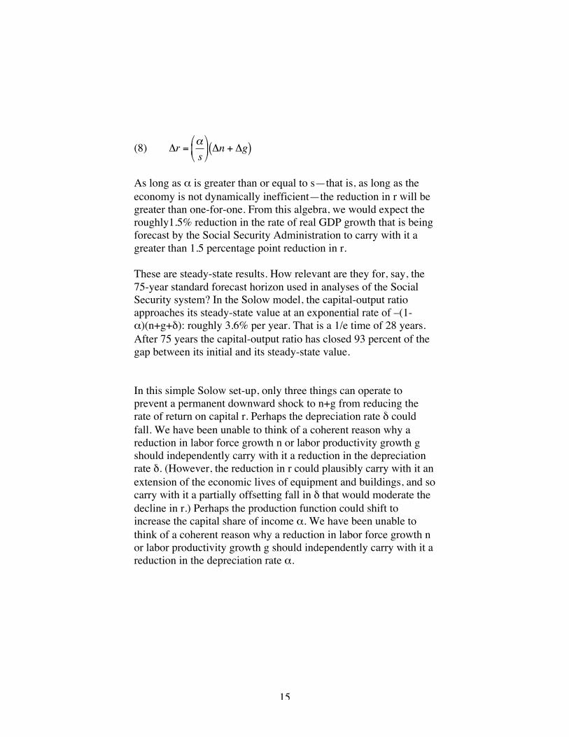
(8)

€

Δr =αs

Δn + Δg( )

As long as α is greater than or equal to s—that is, as long as theeconomy is not dynamically inefficient—the reduction in r will begreater than one-for-one. From this algebra, we would expect theroughly1.5% reduction in the rate of real GDP growth that is beingforecast by the Social Security Administration to carry with it agreater than 1.5 percentage point reduction in r.

These are steady-state results. How relevant are they for, say, the75-year standard forecast horizon used in analyses of the SocialSecurity system? In the Solow model, the capital-output ratioapproaches its steady-state value at an exponential rate of –(1-α)(n+g+δ): roughly 3.6% per year. That is a 1/e time of 28 years.After 75 years the capital-output ratio has closed 93 percent of thegap between its initial and its steady-state value.

In this simple Solow set-up, only three things can operate toprevent a permanent downward shock to n+g from reducing therate of return on capital r. Perhaps the depreciation rate δ couldfall. We have been unable to think of a coherent reason why areduction in labor force growth n or labor productivity growth gshould independently carry with it a reduction in the depreciationrate δ. (However, the reduction in r could plausibly carry with it anextension of the economic lives of equipment and buildings, and socarry with it a partially offsetting fall in δ that would moderate thedecline in r.) Perhaps the production function could shift toincrease the capital share of income α. We have been unable tothink of a coherent reason why a reduction in labor force growth nor labor productivity growth g should independently carry with it areduction in the depreciation rate α.

16

Last, perhaps a permanent downward shock to n+g could alsocarry with it a reduction in the savings rate s. If it were the casethat:

(9)

€

ds = −s

n + g + δ

dn + dg( )

then the rate of return r would be constant. There is a reason tothink that a fall in the labor force growth rate n would carry with ita reduction in s: an economy with slower labor force growth is anolder economy with relatively fewer young people and,presumably—if the young do the bulk of the savings—a lowersavings rate. (A decline in g, however, would tend to work theother way: the income effect would tend to raise s.) Are sucheffects plausibly large enough to keep the rate of return on capitalconstant as the rate of economic growth? To assess that we need tomodel savings decisions, which requires that we move fromalgebra to analysis.

V. AnalysisThe Ramsey ModelMove from Robert Solow (1956) to Ramsey-Cass-Koopmans (seeRomer (2000). Consider a version of this Ramsey model in whichthe representative household has the utility function:

(10)

€

(1+ β)−t U Ct( )( )t= 0

∞

∑ Nt1−λ

Where β is the pure rate of time preference, Ct is consumption perhousehold member, and Nt is the number of members of therepresentative household, growing according to:

(11)

€

Nt+1 = (1+ n)Nt

17

In the standard Ramsey-model setup, the parameter λ is equal tozero: the household utility function is:

(12)

€

(1+ β)−t U Ct( )( )t= 0

∞

∑ Nt

This choice drives the result that changes in labor-force growth donot have long-run effects on steady-state capital/output ratios orrates of return. But, to us at least, this assumption seems artificial.If it is indeed the case that the utility function is (12) above, thenthe more members of the household the merrier: household utilityis linear in the number of people in the household but suffersdiminishing returns in per-capita consumption. A household withthis utility function that had control over its own fertility wouldchoose to grow as rapidly as possible: that would be the way tomake individual units of consumption contribute as much aspossible to total household utility.

It seems reasonable to allow λ to be greater than zero, and so havea utility function which has diminishing returns both with respectto household per-capita consumption and with respect to householdsize.

There is another reason to be uncomfortable with the assumptionthat λ=0. If the term, “golden rule” were not already taken in thegrowth theory literature, we would use it here, for λ=0 requiresthat those household makers making decisions in period t loveothers (the new household members joining in period t+1) as theylove themselves. They assemble the household utility function bytreating the personal utility that others receive in the future fromtheir per capita consumption as the equivalent of their ownpersonal utility. But we can’t call this the “golden rule,” all we cando is call this perfect familial altruism. If λ>0 but less than one,there is imperfect familial altruism—those making period-t

18

decisions care about the personal utility of extra family members inperiod t+1, but not as much as they care about their own. And ifλ=1, period t decision-makers act as if they care only about theirown personal utility. We are comfortable with altruism; we areuncomfortable with perfect familial altruism:

In this version of the Ramsey-Cass-Koopmans model, the first-order condition for the representative household’s consumption-savings decision is:

(13)

€

U '(Ct )dCt =(1+ n)1−λ

(1+ β)U '(Ct+1)dCt+1

If the household faces a net rate of return on financial investmentsof rf, then:

(14)

€

1+ rf1+ n

dCt = dCt+1

because period t+1 resources must be split among more membersof the expanded household.

For log utility, we then have:

(15)

€

Ct+1

Ct

=(1+ n)1−λ(1+ rf )(1+ n)(1+ β)

Along the economy’s steady-state growth path with per-workerconsumption growing at the rate of labor augmentation g, thisbecomes:

(16)

€

rf = (1+ g)(1+ n)λ(1+ β) −1

And in the continuous-time limit:

19

(17)

€

rf = β + g + λn

Looking across steady-state growth paths, reductions in the rate ofoutput per worker growth g reduce rf one-for-one in the case of logutility. (They reduce rf by a multiplicative factor γ of the change ing in the case of constant relative risk aversion utility: U(Ct) =[(Ct)1-γ]/[1-γ].) Reductions in the rate of labor force growth n alsoreduce rf except in the case of perfect familial altruism, the case inwhich λ=0. If λ>0 but less than one, the case of imperfect familialaltruism, slower rates of labor force reduce rf, but not one-for-one.And if λ=1, period t decision-makers are not altruistic at all: theyact as if they care only about their own personal utility, andreductions in n reduce rf one-for-one, as reductions in g do in thecase of log utility.

In the case of the Ramsey model, the fact that the model’sdynamics attract it to a balanced-growth steady state and theassumption of the representative agent all by themselves nail downthe relationship between economic growth and asset returns. Insteady-state per capita consumption is growing at rate g, and so therelative marginal utility of per capita consumption one period inthe future is:

(18)

€

(1+ β)−1(1+ g)−1

in the case of log utility. And the rate at which per-capitaconsumption can be carried forward in time is:

(19)

€

(1+ rf )(1+ n)−λ

To drive the rate of return on capital rf away from:

(20)

€

rf = (1+ g)(1+ n)λ(1+ β) −1

20

in a model with log utility and a rate of per-capita consumptiongrowth of g requires that the consumption of those agents marginalin making the period-t consumption-savings decision grow at a ratedifferent than per-capita consumption growth. This requiresheterogeneous agents. And the simplest model with heterogeneousagents that is suitable is the Diamond model.

The Diamond ModelIn the overlapping-generations Diamond model, each agent livesfor two periods, works and saves when young, and earns returns oncapital and spends when old. Thus for a given generation that isyoung in period t, their per-capita labor income when young wt,their per-capita consumption when young cyt, their per-capitaconsumption when old cot+1, the net rate of return on capital rt+1,and the economy’s period-t+1 per-capita capital stock kt+1 are alllinked:

(21)

€

wt = cyt + kt+1

(22)

€

cot+1 = 1+ rt+1( )kt+1

With a Cobb-Douglas production function, output per (young)capita when the period-t generation are young—in period t—is:

(23)

€

yt = Et1−α kt

1+ n

α

where E is our measure of the efficiency of labor, growing atproportional rate g each period, and where the (1+n) appears in thedenominator because n is the per-generation rate of populationgrowth. With this production function, labor income is a constantfraction of output per capita:

21

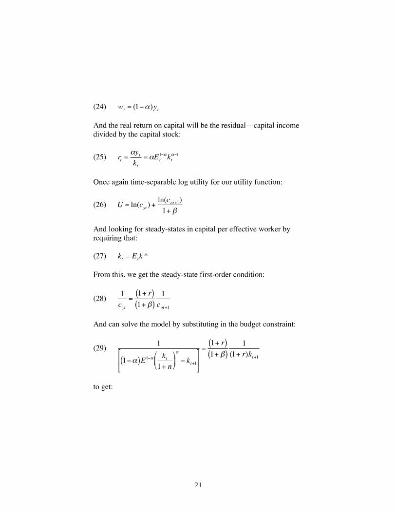
(24)

€

wt = (1−α)yt

And the real return on capital will be the residual—capital incomedivided by the capital stock:

(25)

€

rt =αytkt

=αEt1−αkt

α−1

Once again time-separable log utility for our utility function:

(26)

€

U = ln(cyt ) +ln(cot+1)1+ β

And looking for steady-states in capital per effective worker byrequiring that:

(27)

€

kt = Etk *

From this, we get the steady-state first-order condition:

(28)

€

1cyt

=1+ r( )1+ β( )

1cot+1

And can solve the model by substituting in the budget constraint:

(29)

€

1

1−α( )E1−α kt1+ n

α

− kt+1

=1+ r( )1+ β( )

1(1+ r)kt+1

to get:

22

(30)

€

11−α1+ g

k *1+ n

α

− k *

=1

1+ β( )k *

which leads us to:

(31)

€

k* =1−α( )

1+ g( ) 1+ n( )α (2 + β)

11−α

And, recalling that r = αk*α-1:

(32)

€

r =α 1+ g( ) 1+ n( )α (2 + β)

1−α( )

Analysis: ConclusionThus in the Diamond overlapping-generations model as well as inthe Ramsey model and the Solow model, slower economic growthcomes with lower net returns on capital rf. In both the Diamondand the Ramsey model, there is reason to think that reductions inlabor productivity growth have a greater effect on rates of returnthan do reductions in labor force growth, :

• In the basic Solow algebra, the reduction in gross returns ris proportional to (α/s) times the reduction in growth.

• In the Diamond model, the reduction in net returns rf isequal to (α/(1-α)) times the reduction in labor productivitygrowth g and, to first order, equal to (α2/(1-α)) times thereduction in labor force growth n.

• In the Ramsey model, the reduction in rf is equal (with logutility) to the reduction in labor productivity growth g and,to first order, to λ times the reduction in labor force growth

23

n (where λ is the degree to which familial altruism isimperfect).

At some level, the same thing is going on in all three setups—inthe simple algebra of Solow and in the analyses of Ramsey andDiamond. Reductions in economic growth in these setups are alldeclines in the rate of growth of effective labor relative to thecapital stock provided by previous investments. Effective laborbecomes relatively scarcer, and capital becomes relatively moreabundant. The terms of trade move against capital—and so thereturn to capital falls.8

These models say that there is some economic reason to believethat a slowdown in economic growth would carry a reduction inasset returns with it.

But even though these models are the standard models thateconomics graduate students and their professors use for theirfinger exercises. We are leery of putting too much weight on them.They are oversimplified. They are abstract. They are ruthlesslynarrow in their conceptions of human motivation and institutionaldetail. Their relevance to the real world is something that isasserted by professors in economic theory courses—not somethingthat has been successfully and convincingly demonstrated.

8 Why, then, does a fall in labor force growth not reduce rates of return in theRamsey model in the case of perfect familial altruism? Because a reduction inpopulation growth also reduces the utility value of moving consumption forwardin time—an important component of the value of saving in the Ramsey modelwith perfect familial altruism comes from the possibility of dividing the savingamong more people in the future and thus escaping the diminishing marginalutility of consumption. Thus the marginal household utility of saving falls in theRamsey model when population growth falls. This reduces the effective supplyof capital by as much as the fall in population growth reduces the effectivesupply of labor.

24

Therefore we tend to put more weight on the arithmetic than on theanalysis. We believe in the flow of funds and in payout ratios andgrowth rates more than we believe in simple growth theory. It is,however, important to note that section III and sections IV and Vof this paper have answered different questions. Section III askedwhether, conditional on current asset valuations and on therationality of financial markets, forecasts of slower growtharithmetically entailed forecasts of lower equity returns as well.Sections IV and V have asked the unconditional question: withoutconditioning current asset market valuations, what would weexpect the relationship between growth and asset returns—anaverage of bond and stock returns—to be?

Moreover, the analysis of sections III-V has assumed a closedeconomy. How do the conclusions change when we consider anopen United States economy embedded in a world that has thepotential to grow more rapidly?

VI. The Open-Economy CaseReturn to the steady-state Gordon equity-valuation equation, whereP is the price of a stock index, D and B are dividends and netbuybacks, respectively, and gk is the permanent rate of growth ofpayouts, of earnings, and of the value of the capital stock:

(33)

€

re =D+ BP

+ gk

In the open-economy case gk is not the rate of growth of thedomestic corporate capital stock. It is the rate of growth of thecapital stock owned by American companies. If foreign companieson net invest in America—if the U.S. on average runs a currentaccount deficit—then the rate of growth of the earnings ofAmerican companies in our domestic stock-market index will beslower than the rate of growth of economy-wide earnings and of

25

real GDP. The open economy will then deepen rather than resolvethe problem of combining slow expected growth with highexpected returns. If it is American companies that on net investabroad—then the rate of growth of the capital stock and thus theearnings of companies in the index will be larger than the rate ofgrowth of the domestic economy g.

How much larger? If we look over spans of time long enough foradjustment costs in investment not to be a major factor, then thevalue of the capital stock will be proportional to the size of thecapital stock.9 If we assume in addition that companies maintainstable debt-equity ratios, then we have:

(34)

€

gk = g + x YK

where x is that component of the current-account surplus (as ashare of GDP) that corresponds to American companies’ netinvestments abroad,10 and Y/K is the current output-to-corporatecapital ratio.

Here, again, we return to arithmetic. Our rate of equity return is: 9 Note that we here dismiss the possibility that investments overseas mightprovide higher risk-adjusted rates of return in the long run than domesticinvestments: Tobin’s q=1 both here and abroad. The BEA reports that as of theend of 2003 the market value of foreign direct investment in the United States is$9,166.7 billion, compared to direct investment abroad by U.S. corporations of$6,369.7 billion, yet the associated income flows are about the same. Weattribute this to a difference in risk. The experience of nineteenth century Britishinvestors with such landmarks of effective corporate governance as the ErieRailroad suggests that while there are supernormal returns to be earned in thecourse of rapid economic development, people with offices separated by oceansare unlikely to be the ones who reap them.

10 The phrase “corresponds to American companies’ net investment abroad” isneeded to abstract from current-account deficits that finance net governmentconsumption or net household consumption

26

(35)

€

re =D+ BP

+ g + x YK

From section III, this is:

(36)

€

re = 4.5% + x YK

For a capital-output ratio of 3, we then have:

(37)

€

x = 3(re − 4.5%)

Determine how much you want the rate of return on equities toexceed the 4.5% per year closed-economy benchmark casecalculated in section III, and triple that: that is the current-accountsurplus associated with net corporate investment overseas neededto produce the higher return.

Note that, for a constant rate of return, the needed surplus x growsover time. In equation (37), Y/K is not the physical domesticoutput-to-capital ratio: it is the ratio of domestic output to totalAmerican company-owned capital—including capital overseas. Asoverseas assets mount, the needed surplus for constant payoutyields mounts as well.

Now such enormous current-account surpluses are possible. GreatBritain had them in the quarter-century before World War I, whenit ceased to be the workshop of and became for a little while thefinancier of the world (see Edelstein (1973)). Slowing economicgrowth in the late Victorian and Edwardian eras and reducedinvestment relative to national savings was cause (or consequence,or both?) of the direction of Britons’ saving and of Britishcompanies’ investment overseas. We, however, see no signs thatthe United States will undertake a similar trajectory over the next

27

several generations. And we are impressed by the scale: to beconsistent with current payout yields, the 1.9% per year forecastreal GDP growth rate, and 6.5% returns the current account surplusproduced by American net corporate investment abroad wouldhave to begin at 6% of GDP, and grow thereafter.

Moreover, the assumption that America could cope with slowingeconomic growth and maintain domestic asset returns at highhistorical average levels by diverting capital overseas rests, tosome degree, on the belief that the United States is a small openeconomy: that U.S. investments abroad induced by a domesticgrowth slowdown will raise the rate of return here while notlowering rates of return there. But the U.S. is not a small openeconomy. It is a large open economy. Blanchard, Giavazzi, andSa’s (2005) estimates are that U.S. financial assets are currentlyhalf of the world total. This share will fall over time. But fastenough to make the assumption that the U.S. is a small openeconomy a reasonable approximation?

We doubt it. Once again, the potential escape from arithmetic andanalysis seems to us to be a possible scenario, but not the centraltendency of the distribution of possible futures that is a forecast.

VII. The Equity PremiumEconomists do not have a good explanation of the equity premium.Rajneesh Mehra and Edward Prescott (1985) is entitled, “TheEquity Premium: A Puzzle,” for good reason. Stocks haveoutperformed fixed-income assets by more than 5% per year as farback as we can see. As Martin Feldstein has said in conversation,it’s as if the market’s attitude toward systematic equity risk is thatof a rich 65 year old male with a not-very-healthy lifestyle whosedoctor has told him that he is likely to live less than a decade. Yetwe believe that properly-structured markets should—andcan—mobilize a much deeper set of risk-bearers with a much

28

greater risk tolerance. That they do not appear to have done so is asignificant mystery.

One potential explanation is that the extremely large equitypremium is a thing of the past, not the future.11 In the distant pastfear of railroad and other “robber baron” scandals, and in the morerecent past the memory of the Great Depression kept someexcessively averse to stocks. In addition, the U.S. had remarkablygood economic luck. And, over time—as people realized that theirpredecessors had been excessively averse to equity risk—risingprice-dividend ratios pushed a further wedge between stock andbond returns. But today the arithmetic of section III gives us stockreturns of 4.6%: an equity premium of perhaps 2.5 percentagepoints, not 5.

To the extent to which this past behavioral anomaly was the resultof an excess fear of stocks and an excess attachment to bonds, it isnot clear that its erosion should have an impact on the expectedreturn on a balanced portfolio. The simplest, crudest, and mostextremely ad-hoc model of the equity premium would embed thestock-vs-bond investment decision in the simplest possibleDiamond-like OLG model, with the capital stock each period beingthe wealth accumulated when young by the old, retired generation.Assume that each generation, when it saves, invests a share eh ofits savings in equities and a share 1-eh in bonds. Firms, however,are unhappy with such a capital structure. Unwilling to runsignificant risks of bankruptcy, they are unwilling to commit lessthan a share ef, where ef > eh of their payouts to equity. A smallercushion—in the sense that a smaller cyclical decline in relativeprofits would run the risk of missing bond payments and anappointment with a bankrupty court—is simply unacceptable toentrenched managers.

11 In conversation Randall Cohen has been an especially forceful advocate ofthis point of view.

29

If a physical unit of savings when young yields returns to physicalcapital 1+r when the savers are old, the rates of return on equityand debt are then:

(38)

€

1+ re = (1+ r)e feh

and:

(39)

€

1+ rd = (1+ r)1− e f1− eh

with the equity premium being:

(40)

€

1+ re1+ rd

=(eh /(1− eh ))(e f /(1− e f ))

In this excessively-simple framework it does seem highly plausiblethat eh has fallen with greater household willingness to holdequity—whether because of institutional changes, the fadingmemory of 1929, two decades of fabulous bull markets, orincreased financial sophistication on the part of households. Thuseven if there were no reasons connected with slowing growth toexpect lower returns on capital, one might well expect to see lowerreturns on equity in the future than in the past. And we have seenthe major institutional changes that we would expect, from abehavioral perspective, to boost the share of financial assetsnaturally channeled to equities: the rapid expansions of taxpreferences for financial savings vehicles and the growth of 401(k)and other defined-contribution pension plans have been importantparts of the last generation’s changes in financial markets (seeBarberis and Thaler (2003)).

30

A lower rate of return on the assets in a balanced portfolio haspowerful implications on issues of economic policy. A lowerequity premium seems to us at least to have powerful implicationsfor only one issue: whether there is a large market failure in thestock market’s apparent inability in the past to mobilize a largeshare of society’s potential systematic risk-bearing capacity, andwhether a government-run social insurance scheme can and shouldattempt to profit from and to at least partially repair this failure tomobilize society’s risk-bearing resources. The government, afterall, has the power to tax: it has the greatest ability to managesystematic risk of any agent in the economy. If others are notpicking up their share—and if as a result there are properlyadjusted excess returns to be earned by the government’s taking adirect position itself or assuming an indirect position by reinsuringindividuals’ social-insurance accounts—why should thegovernment not do so? The difference between the economists ofthe coast and the economists of the interior is that the firstspecialize in thinking up clever schemes to repair apparent marketfailures and the second specialize in thinking up clever reasonswhy apparent market failures are not really so. Even though we arefrom the coasts, we find that there are enough reasons to believethat the equity premium will be smaller in the future than in thepast to wish that attempts to exploit the equity premium beimplemented slowly and gingerly.

VIII. ConclusionEconomic growth here at home is determined by productivitygrowth and labor force growth here in the United States. Equitymarket and other asset returns determined by the overall cost ofcapital in the global economy and by the return investors require tobear the risk that comes with equity ownership. Yes. But. TheUnited States is not a small open economy in which these two setsof factors are not linked. The United States is a large openeconomy, and so we would expect that shifts in the economy that

31

reduce the rate of economic growth would be accompanied byreductions in the rate of return on assets as well.

We would expect the reduction in asset returns to be greater forreductions in productivity growth than for reductions in labor forcegrowth. We think that this reduction in asset returns could be offsetand neutralized by other factors—if there is a successful class warwaged by capital against labor, if today’s stock market values arenot sober reflections of likely returns but are elevated by irrationalexuberance, or if the United States cuts its consumption beneath itsproduction for generations and follows Britain’s pre-WWItrajectory as supplier of capital to the world. Nevertheless, we seethese as unlikely (thought possible) scenarios. We do not take anyof them—or some combination—to be the central tendency of thedistribution of possible futures that is a proper economic forecast.

What, some have asked, is the relationship between our arithmeticdemonstrations that equity returns as high in the future as in thepast are unlikely and our analytical arguments that rates of returnand rates of growth are likely to move together. We see these twostrands as reinforcing each other. Returns must be consistent withthe savings decisions of households, the investment decisions offirms, and the technologies of production. But it is also the casethat returns must also equal payout yields plus capital gains—andthat only in stock market bubbles can capital gains divorcethemselves from economic growth, and then only for a little while.

Once again, return to our perhaps useful analogy from internationaleconomics. Given prices charged by foreigners, domesticconsumers decide on how much of imports M to purchase; givenprices charged by domestic firms, foreign consumers decide onhow much of exports X to purchase; why then do we say that thetrade balance X-M is determined by the national savings-investment balance, that X-M=S-I? The answer is that powerfuleconomic forces work to make sure that what the economy’sbehavioral relationships produce is consistent with its equilibrium

32

flow-of-funds conditions. The same general logic applies here: Ifslower economic growth reduces the arena for the profitabledeployment of capital, rates of return will fall until less capital isdeployed. By how much will they fall? Until—in steadystate—payout yields plus retained earnings are equal to profits, andretained earnings are no larger than the sustainable growth of thecapital stock permits.

References

Nicholas Barberis and Richard H. Thaler (2003), “A Survey ofBehavioral Finance,” in Constantanides, Harris, and Stultz, eds.,Handbook of the Economics of Finance (Amsterdam: Elsevier).

Olivier Blanchard, Francesco Giavazzi, and Filipa Sa (2005forthcoming), “The U.S. Current Account and the Dollar,”Brookings Papers on Economic Activity.

Council of Economic Advisers (2005), “Three Questions AboutSocial Security” http://www.whitehouse.gov/cea/three-quest-soc-sec.pdf

Peter Diamond (1965), “National Debt in a Neoclassical GrowthModel,” American Economic Review, 55, 1127-1155.

Peter Diamond (2000), “What Stock Market Returns to Expect forthe Future?” Social Security Bulletin 63:2, pp. .38-52.

Michael Edelstein (1973), Overseas Investment in the Age of HighImperialism (Cambridge: Cambridge University Press).

33

Robert Gordon (2003), “Exploding Productivity Growth: Context,Causes, and Implications,” Brookings Papers on Economic Activity2003:2.

Michael Kremer (1993), “Population Growth and TechnologicalChange: One Million BC to 1990,” Quarterly Journal ofEconomics (August), pp. 681-716.

Rajneesh Mehra and Edward Prescott (1985), “The EquityPremium: A Puzzle,” Journal of Monetary Economics

Steven Oliner and Daniel Sichel (2003), “The Resurgence ofGrowth in the Late 1990s: Is Information Technology the Story?”UPDATED (Washington: Federal Reserve Board).

David Romer (2000), Advanced Macroeconomics, 2nd ed. (NewYork: McGraw-Hill).

Jeremy Siegel (2005), The Future for Investors (New York: CrownBusiness: 140008198X).

Social Security Administration (2005), Trustees’ Reporthttp://www.ssa.gov/OACT/TR/

Robert Solow (1956), “A Contribution to the Theory of EconomicGrowth,” Quarterly Journal of Economics.