forecasting framework for inventory and sales of short
TRANSCRIPT

Forecasting Framework for Inventory and Sales of
Short Life Span Products
Master Thesis
Graduate student: Astrid Suryapranata
Graduation committee:
Professor: Prof. dr. ir. M.P.C. Weijnen Supervisors: dr. ir. Zofia Verwater-Lukszo Scott W. Cunningham D.Phill
Clive Marshmandr. ir. Ardjan Krijgsman
Technology and Policy Analysis Delft University of Technology
2003

i
Executive Summary Forecasting is used to predict or describe what will happen, and the use of such forecasts in planning would help in making a good decision about the most attractive alternatives for the company. The forecasting tasks is even more important in developing a new product since the actual sales performance of this new product has not been known, while many decisions should be made to manage the product into a desired growth. This situation is faced by Unilever as it has just started developing new products which have a short life span characteristic. This characteristic is a new experience for the company to cope with. The excess stock tolerance of this type of product is smaller than of the non-perishable products, while out of stock condition has never been an option in the company’s policy for any type of its product. This leads the company to consider having a ‘good’ forecasting. Therefore, this research is conducted as an attempt to seek what forecasting techniques are appropriate to support decisions making in the operational level of supply chain when dealing with short life span products to avoid undesired stock conditions.
To answer this question, literature study of forecasting and information gathering about the current forecasting practices are done during the research. The literature study provides knowledge about the forecasting method ranges and their applications. Whilst, studying the current forecasting practices gives knowledge about what have been done in the company and the company’s expectations with respect to this matter. The company’s expectations are related to the general objectives of the forecasting process which is described through an objective tree approach and the solutions for the company’s specific forecasting problems which are identified through a system diagram and causal diagram approaches.
The main general objective of the forecasting process is determined in the objective tree, which is to have a good forecasting. The next is to perform further decomposition of the main general objective into the sub objectives that contributing to it in order to determine the forecasting specification. This functional specification results in a fact that forecast accuracy is not the only important parameter. Practical factors are also expected to be considered in selecting the forecasting techniques, for examples the easiness of using the method and the easiness of understanding the model. It creates a possible trade off between forecast accuracy and ‘simplicity’ of the method/model.
System diagram and causal diagram approaches are used to identify the possible forecasting problems. The system diagram is aimed to help focusing and demarcating the problem area for this study by determining the boundaries of the forecasting system. Next, the causal diagram is developed to define the relationships underlying the forecasting processes and to find the variables involved in it. The system diagram identifies three potential outcomes of interests, while the causal diagram determines the forecasting problems that correspond to those outcomes of interests. The identified forecasting problems are the sales order, the inventory and the product availability in the market forecasts. This problem identification leads to an attempt finding forecasting methods that are suitable for each of it and results in proposing three forecasting methods accordingly. The methods are Winters Exponential Smoothing for sales order forecasting, MARIMA model for inventory forecast and system dynamics approach for forecasting the product availability in the market.
An accurate sales order forecast for an individual item is required to support the company in making decisions related to production operations for the production scheduling purpose in managing short life span products. Besides the accuracy parameter, the method should be able to handle seasonality and trend factors as presumed to consist in the demand of the products of interest. It should also be able to handle daily sales for item unit level. Conducting literature analysis directs to conclude that Winters’ Exponential Smoothing Method is suitable for dealing with these requirements. The finding from a famous comprehensive empirical study, the M-competition, proves that this method performs well in term of accuracy when competed with other forecasting methods. Also, this method is aimed to handle seasonality and trend factors and its simplicity enables this method to handle daily data for item level.
To avoid the undesired stock conditions when dealing with short life span products, having only a good sales forecasting is insufficient because the stock conditions are resulted from supply chain processes such as production and delivery in which indeed driven by the sales order. In this case, the company

ii
should also manage the stock availability in the distribution center as well as in the market, especially in the channels in which the company has more direct control. For that purpose, two forecast methods are suggested which are MARIMA (Multivariate Auto Regressive, Integrated, Moving Average) method to control the inventory and system dynamics approach for controlling the product availability in the market.
The MARIMA (Multivariate Auto Regressive, Integrated, Moving Average) model is proposed to forecast the daily stock availability for the aggregate level of product which incorporates the sales order quantity, production quantity and delivery quantity factors with time lags. This method is chosen due to its ability to model the time lags which typically involved in the control process. The result of the inventory forecast will be compared to the daily inventory target, which is ‘zero’ – as low as possible – inventory for short life span products. This enables the company to take necessary actions when the predicted inventory result is undesirable. This MARIMA model is used to forecast the inventory in the aggregate product level since the complexity of the development such a model for item level would result in an inefficiency of maintaining different model for different item. In addition to that, the appropriate level of setting the target inventory is in the aggregate level because the target is ‘zero’ – as low as possible – inventory for the overall short life span products.
In dealing with short life span products, the distribution chain should be designed as short as possible to maintain the freshness of the product. To do so, the company should aware that the product availability in the market is the result of complex relationships among factors in the supply chain operation with feedback relations. It directs to suggest using the system dynamics approach which includes the production, inventory, distribution and forecasting processes to control the product availability in the market. The ability of system dynamics approach to present the predicted future behavior when a decision is taken upon one or more factors in the system enables this approach to support the company in policy decision making with respect to the production, inventory and product availability in the market. Some examples of the possible policies that identified in this study are reducing desired safety stock level, increasing the frequency of replenishment cycle, reducing order processing time and a combination of reducing safety stock level and reducing order processing time.
Finally, as an attempt to improve the forecasting result, an analysis of the organizational arrangement around the forecasting process is performed. This results in identification of the condition under which a forecast revision is allowed, of the people involved, of the method used in making a decision and of the information management in qualitative analysis forecasting process. This qualitative analysis should only be performed in the situation to which a ‘substantial’ change is expected that cannot be incorporated in the quantitative forecasting method to avoid the risks of inconsistency and biases.
A combination of the Jury of Executives Opinions and the Sales Force Composite method is proposed. The Jury of Executives Opinion approach is applied when revising the forecasting results in the aggregate product level, while the Sales Force Composite approach should be applied to decompose the forecast in the aggregate level into the appropriate lower level. The people involved in the judgmental forecasting should satisfy a minimum level of knowledge and experiences and also should posses a ‘similar’ capacity in their departments in order to maintain the ‘balance’ of the group. Equal weight assessment of the forecasts that addressed by each group member in achieving consensus for the final forecasting results is suggested. Information of the forecast outcomes which are resulted from the quantitative method as the forecast base and a relevant contextual information about the influencing factors should be provided and the data should be presented in the correct manner such as graphical presentation for trended data and tabular for non-trended data. Feedback of the forecasts as soon as the actual value is available should also be given to the people involved in forecasting and all information should be properly recorded for future improvement.
In brief, this study presents a framework of forecasting for sales and inventory of short life span products which includes sales order forecasting using Winters Exponential Smoothing method, inventory forecasting using MARIMA model and product availability forecast using system dynamics approach. In addition to that, a qualitative analysis for sales order forecasting is also presented as an attempt to improve the accuracy of sales order forecast when an ‘abnormal’ condition occurred that cannot be incorporated in the quantitative forecasting method.

iii
Acknowledgments
This report has been made in order to finalize the thesis assignment that had been performed at the Faculty of Technology and Policy Analysis at TU Delft, in collaboration with Unilever Research and Development, Vlaardingen, the Netherlands. It describes the results of my master thesis project within the framework to develop a forecasting concept design for inventory and sales of short life span products.
I would like to thank all the members of the committee who have already given their expertise to the improvement of this thesis and not to mention my personal and academic development, my attitude and my competence in the working field.
I would like first to thank Prof. Margot Weijnen who serves as the chairperson of the thesis committee for her encouragement and significant feedback in the completion of this thesis.
I would like to thank my first supervisor, dr. ir. Zofia Verwater-Lukszo for giving me opportunity to carry out this thesis in the Energy & Industry section at the first place. Furthermore, I would also like to thank her for her feedback, encouragement, guidance and attention during this study. I realize that without her kind attention, patience, and ‘motherly’ touch in supervising me, I would not have been so motivated to do my best in the thesis project.
I would like to thank my second supervisors, Scott W. Cunningham, D.Phill, with his idea and knowledge that challenge me to explore some aspects in the study more deeply. His patience during the discussion has valuable contribution to the completion of this work.
I would like to thank Clive Marshman and dr. ir. Ardjan Krijgsman from Unilever R&D, Vlaardingen, for giving me the opportunity to carry out this thesis project in the company. I would like to thank for their time, inputs, and all of the facilities I got during the internship period. Moreover, I would also like to thank all colleagues in Unilever R&D, Vlaardingen, for their hospitality during my internship period.
I would like to thank all who have been supporting me with their endless prayer, encouragement and support, especially my parents, family and fiancé for without them I would not have been always cheerful during my study period. I also wish to extent my thanks to my brothers and sisters from BIC Den Haag and CWS Kharis whom I know had supporting me with their continuous prayer. I would also like to thank all of my friends from TU Delft for their encouragement and support during the project, moreover, during my study period in TU Delft.
Above all, I will give thank and praise to the Lord for His endless love and faithfulness. “Things which the eye saw not, and which had not come to the ears or into the heart of man, such things as God has made ready for those who have love for Him” – (1 Corinthians 2:9).
Delft, August 5th, 2003
Astrid Suryapranata

iv
Table of Contents page
Executive Summary ...................................................................................................................i Acknowledgments ................................................................................................................... iii Table of Contents .................................................................................................................... iv Chapter 1. Introduction.............................................................................................................1 1.1. Forecasting Role and Practice in Business ...........................................................................1 1.2. Background of the Problem ...............................................................................................1 1.3. Forecasting Practices in the Company.................................................................................2 1.4. Thesis Assignment and Research Questions ........................................................................3 1.5. Research Approach...........................................................................................................4 1.6. Layout of the Report .........................................................................................................6 Chapter 2. Analysis of the Existing Forecasting Methods ..............................................................8 2.1. Quantitative Forecasting Methods ......................................................................................8 2.2. Qualitative Forecasting Methods.......................................................................................17 2.3. Integration of Quantitative and Qualitative Forecasting Methods.........................................20 Chapter 3. Formulation of the Forecasting Problem ...................................................................25 3.1. Problem Outline..............................................................................................................25 3.2. Forecasting Functional Specification .................................................................................25 3.3. Forecasting Variable Specification ....................................................................................27 3.4. General Remarks on Model Choices..................................................................................35 Chapter 4. Sales Forecasting Model Using Winters’ Exponential Smoothing ..................................38 4.1. Introduction ...................................................................................................................38 4.2. General Requirements.....................................................................................................39 4.3. General Structure ...........................................................................................................40 4.4. Application of the Model in Unilever Case..........................................................................45 4.5. Final Remarks ................................................................................................................49 Chapter 5. Inventory Forecasting Using MARIMA (Multivariate Auto Regressive, Integrated, Moving
Average) Model ..............................................................................................................51 5.1. Introduction ...................................................................................................................51 5.2. General Requirements.....................................................................................................51 5.3. General MARIMA Model...................................................................................................53 5.4. Application of the Method to Unilever Case .......................................................................59 5.5. Final Remarks.................................................................................................................66 Chapter 6. Product Availability Forecasting Model Using System Dynamics...................................69 6.1. Introduction ...................................................................................................................69 6.2. General Requirements.....................................................................................................69 6.3. General Structure of System Dynamics Model....................................................................70 6.4. Application of the Model to Unilever Case .........................................................................71
6.4.1. Problem Identification .....................................................................................71 6.4.2. Model Conceptualization ..................................................................................72 6.4.3. Model Formulation ..........................................................................................76
6.4.4. Simulation Result and Model Behavior...............................................................83 6.4.5. Model-Based Policy and Scenario Analysis .........................................................83 6.5. Final Remarks ................................................................................................................84 Chapter 7. Integration of Quantitative Models with Qualitative Analysis .......................................86 7.1. Introduction ...................................................................................................................86 7.2. General Requirements.....................................................................................................86 7.3. Implementation..............................................................................................................87 7.4. Final Remarks ................................................................................................................90 Chapter 8. Final Considerations................................................................................................92 8.1. Conclusions....................................................................................................................92 8.2. Recommendations ..........................................................................................................94 8.3. General Remarks ............................................................................................................95 References.............................................................................................................................97

1
Chapter 1. Introduction
1.1. Forecasting Role and Practice in Business
The role of forecasting within a business is varied. It depends upon the time horizon and the functional areas to which the forecast relates (Makridakis and Wheelwright, 1989). Nevertheless, it is important in a wide range of planning and decision-making situations.
Forecasting is used to predict or describe what will happen, and the use of such of forecasts in planning would help make a good decision about the most attractive alternatives for the company (Makridakis and Wheelwright, 1989). For instance, sales forecast would enhance the decision quality of a sales strategy performed by the sales or marketing department. The same sales forecast would also be used by operational departments for supporting a decision on planning and scheduling of production process. Moreover, this forecast would be used by financial department in order to plan a decision on sales revenue, inventory level, et cetera.
Therefore, a wrong forecast will lead to a low quality of decision. Considering the cost that a company should pay as the result of a wrong decision, such as obsolete products due to over stock or opportunity cost due to out of stock in crucial time, there is no doubt that forecasting is important. On the other hand, it is also sensible that low forecast quality allows people to discount the use of this sort of forecast in a decision making.
In a new product or service development situation, the ability to forecast is even more important since the actual performance of the new product or service has not been known while many decisions should be made to manage the product or service into a desired growth. Decisions would highly be driven by forecast result. Thus, a good forecast, which is able to predict the realistic future, is highly desired in order to manage the new product or service development into success.
Many forecasting techniques have been developed either quantitative or qualitative methods. In fact, the most common practice in business is the judgmental forecasting method (Makridakis 1989, DeLurgio, 1998, Wright & Goodwin 1998) in which the decision-makers perform a forecasting task through a judgmental decision mainly based on their intuitions and experiences. Almost all enterprises have experienced in accomplishing forecasting task through judgmental method, some perform with the combination of statistical method and only few rely solely on the statistical method (Makridakis, 1989). Since human judgment is prone to biases and inconsistency (Wright & Goodwin, 1998) thus it should be aware of the risks of performing forecasting task through this method when the technique in accomplishing the forecasting task is inappropriate. The risk involved is reducing the quality of a decision due to poor forecast. Nevertheless, a judgmental forecasting done by experts might be advantageous to some extent.
As the conclusion, since forecast can be considered as inputs for a strategic as well as operational planning within an industry, a ‘good’ forecast is fundamental in order to enhance planning decision.
1.2. Background of the Problem
Unilever business has just started a development of refrigerated prepared food products which they call chill products. These products, such as sandwiches and salads, are distributed through various vending channels, for instance a cold vending machine or a refrigerator placed in a convenience store or a supermarket. The development of this new product is in the preliminary stage and the company desires to explore the possibilities to expand and grow this particular product category. The current existing product that has been launched in the market is sandwich product which is developed under Bertolli brand.

Chapter 1 – Introduction 2
As has been understood, one of the unique characteristics of this kind of products is its life span characteristic. These products have a very short life span compared to other products that have been developed successfully by Unilever. The expected life span in this case is only few days, while most of existing Unilever’s products have a longer life span, say months or even years. Therefore, the development of this kind of product is a new challenge for the company.
This new challenge means that Unilever should be more careful in studying the opportunity in this new business, thus more careful in strategic decisions such as the investment cost or in operational decisions such as the supply chain process design. Those strategic decisions should ensure the achievement of the objective to bring the product into a big success like other Unilever’s products. Considering that forecast is always involved as the underlying factor in making any decision in planning, thus the need of a ‘good’ forecast is inevitable.
Looking back to the reason of new experience in handling such a short life span type of product, the company wishes to have a good forecasting that could be used to support decision making in the operational level of supply chain. For example, to support the company in a decision of production quantity. This is driven in a fact that the tolerance of excess stocks for this type of product is smaller than for a non-perishable product. Besides the obvious risk of financial lost that involved due to an overstock condition, a problem related to an environmental issue may be raised. Meanwhile, out of stock condition has never been an option in the company’s policy for any type of its product at all. Especially in a new development stage, out of stock would harm the product penetration both to the customers and consumers. As a consequence, a good planning with respect to supply chain operation is highly desired in order to manage this new product development into success.
However, to have a good forecasting is not an easy task. First of all, the hard data and information regarding this matter is very limited, or even unavailable. This creates a big challenge to forecast. Moreover, the uncertainty that is always involved in forecasting, for instance people’s behavior in refrigerated prepared food consumption, competitors’ activity, price elasticity, increases the difficulties in forecast these new products.
Therefore, the aim of this research is to develop a forecasting concept that is able to provide a realistic prediction of the future and valuable for users since it supports them in decision making, in particular within the supply chain area. Though many forecasting theories have been developed, however, it is realized that every forecasting method has trade-offs. The first trade-off occurs in accuracy of the method and effort to perform it (Makridakis and Wheelwright, 1989). The more sophisticated the method used, it might provide better accuracy, but it might involve more cost. Another important trade-off occurs in model generality. A more detailed model, with additional forecasting parameters, may provide better forecasts in sample. However, these models are usually less able to generalize out of sample, and to new and unexpected circumstances. Therefore, this study should also take into account these trade-offs, so that the result will be realistic to be applied in the company.
1.3. Forecasting Practices in the Company
The forecasting practice for each of Unilever’s business is not necessarily the same. The type of the product or product category governs how to conduct the forecasting task in practice. However, in general the forecasting practice in Unilever business is divided into 2 phases, which are planning phase and scheduling phase.
Planning Phase
The forecast is started in the beginning of every year. Every brand manager from marketing department will plot their sales target for each product category of each brand for the on-going sales year. This is a very rough forecast and the number will be the total target sales for the total category. The brand managers forecast this target based on the sales achievement of last year and added with marketing activity factor as well as product growth factor.

Chapter 1 – Introduction 3
Scheduling Phase
After the marketing department finishes their forecast planning, they will convey this forecast to sales department. Sales department is responsible to decompose it into more detail forecast, for instance by month, then by week for operation purpose, per product line as well as per SKU.
In breaking down this target into monthly forecast, sales department will use the last year sales achievement figure and marketing activity plan for the current year. They will evaluate last year sales achievement and breakdown the current sales target based on the evaluation of last year sales achievement and incorporate the marketing activity plan for the current year.
During the on going year, this monthly schedule forecast is revised based on the up to date sales achievement. Monthly forecast will be decomposed into weekly forecast for operation purposes, such as supply to customer and order to suppliers (manufacturing). This revision will be based on commercial agreement with Unilever’s suppliers and demand from customers.
1.4. Thesis Assignment and Research Questions
Thesis Assignment
The thesis assignment is performed in Unilever R&D in Vlaardingen, the Netherlands. The objective of this assignment is to deliver a forecasting method design for a refrigerated prepared food product type which appropriate to support the Unilever business in decision making situation with respect to the supply chain operation.
The expected result of this assignment is a forecasting method design for refrigerated prepared food products that incorporates best practices from forecasting theory. This design includes both quantitative and qualitative forecasting methods. At the end of this study, the usage of this forecasting method design will be analyzed in order to evaluate its impact within the business.
Due to limited time available for doing this study, the research will be focus on developing a forecasting method for a refrigerated prepared food product in SKU level (Stock Keeping Unit) which will be applied for a short term planning horizon.
Research Questions
The main question in this research is how to develop an appropriate forecast method for short life span products.
To develop an appropriate forecast, three aspects should be considered. First aspect is correlated with the objectives and goals of the forecasting study, while the others are correlated with the technical and the management parts. This results in the following main research questions for this study:
1. What functional specifications of forecasting are required to yield an applicable forecasting method for the company?
2. What forecasting techniques are appropriate for dealing with uncertainty of demand due to its dynamics and seasonality characteristics?
3. How organization arrangement around the forecasting process should be defined to improve the forecasting result?

Chapter 1 – Introduction 4
1.5. Research Approach
This research is started by performing a literature study of forecasting and finding as much as possible information about the current forecasting practices and about the specific product that being developed. These activities will also be done during performing the project. The approach in conducting this research is divided into 5 parts, which are: conceptualization, specification, solution finding, evaluation, and final consideration part. Figure 1-1 summarizes this approach.
Conceptualization
There are two steps in the conceptualization method, which are as the following.
Identify Problem
Defining the problem is very important in order to solve the right problem. This step involves identifying the questions or issues involves, fixing the context within which the issues are to be analyzed, clarifying constraints and deciding on the initial approach (Walker, 1997).
Specify Objectives
This step describes the requirements to be achieved in the study. An objective setting is important to be performed in order to give direction of the study as well as to evaluate whether a study would have been accomplished successfully. This step also describes the focus of the research.
Specification
Determine Functional Specification
In this step, a set of detail criteria for the forecasting specifications is determined. An objective tree will be used to generate those criteria. The functional specification is performed in order to guide the development of forecasting method into the fulfillment of users’ expectation and help user to understand how a forecast should be evaluated.
Determine Forecast Variables
A system diagram and causal diagram approach would be used to determine variables within the forecasting activity. These diagrams are used to describe the scope of the forecasting system within this study, thus it is able to identify input, output and control variables that are involved in the forecasting system. In this step, the dependent variables and independent variables are specified depending on what to be forecast. Dependent variables are variables that are going to be forecast, while independent variables are additional forecasting parameters that might be incorporated in forecasting. Within this step, a selection of variables should be performed in order to maintain the ‘simplicity’ of the model.
Solution Finding
Develop the Quantitative Forecasting Method
The approach of developing a quantitative forecasting method is presented in Figure 1-2. After the variables to be forecast are determined, using the assumptions of data patterns and relationships together with the forecasting objectives, an analysis of selecting preliminary quantitative forecasting method could be performed. Afterward, the initial data requirement can be specified accordingly to the selected method. This step is followed by gathering initial data. At this point, a data dictionary is created to explain the data elements such as data source, noise of data. It will be used to analyze whether the data is appropriate to be applied in the preliminary chosen forecasting method and whether a corrective action was necessary. When the data is ready, mathematics calculations and statistical tools will be used to determine the patterns or relationships of the data. Determining evaluation parameters will be carried out after the application of the model in the initial data and the accuracy of the application of the model

Chapter 1 – Introduction 5
will be measured afterwards. When the accuracy level and all evaluation parameters satisfy the requirements, this model is ready to be used for out-of sample forecasting.
Integration of the Quantitative Model with Qualitative Analysis
The quantitative forecast models will be integrated with some qualitative analysis in order to achieve better forecasts. The analysis will be started by exploring the possible qualitative influences and how these influences can be incorporated in the quantitative forecasts. This integration process will be explained in a process design which containing the conditions and requirements to which integration is desirable and the best practice procedures of integration to achieve a better forecast.
Figure 1-1. Research Approach
Specification
Solution Finding
ConceptualizationIdentify Problem
Determine FunctionalSpecifications
DevelopQuantitativeForecasting
Method
IntegrateQuantitativeMethod withQualitativeAnalysis
Final Consideration
DetermineForecast Variables
Study CurrentForecasting
PracticeLiterature Review
Specify Objetctives
Evaluation on New Forecasting Design

Chapter 1 – Introduction 6
Evaluation
After the development of the forecasting methods is finished, the methods will be evaluated. In this evaluation part, the advantages and the pitfalls of the selected methods as well as the cost (effort) to develop and use the models will be analyzed by conducting some interview with some people in the company whose tasks related to forecasting or supply chain.
Final Consideration
In this final part, the conclusions, recommendations and final remarks of the study will be presented. The conclusions will be focus on answering the research questions, while improvement recommendations will be presented in the recommendations part. The final remarks will contain some thoughts of the valuable learning and experiences while performing this study.
Figure 1-2. Develop Quantitative Forecasting Method
1.6. Layout of the Report
The thesis report will be arranged in the following manner.
Explanations about the role of forecasting in business, problem identification, the assignment and objectives of the study as well as the approach in conducting this study are presented in Chapter 1.
In Chapter 2 an analysis of the existing forecasting models will be presented. This chapter presents the choices range of the forecasting models and the advantages as well as pitfalls of each of them.
Analyze and SelectInitial Quantitative
Forecasting Method
Specify RequiredData
Gathering InitialData
Determine thePatterns or
Relationships ofthe Initial Data
Accuracy Test
Determine theAppropriateQuantitative
Forecasting Model
DetermineEvaluationParameters
Determine theInitial Forecasting
Model

Chapter 1 – Introduction 7
The specification of the forecasting problem in the company will be presented in Chapter 3. This chapter contains problem description, functional specification and variable specification of forecasting problem. Here also the preliminary choice of the forecasting models will be presented.
Chapter 4 contains the development of the sales forecasting model using Winters’ Exponential Smoothing. This chapter is started with an introduction and followed by an explanation of the general requirements that should be satisfied by this model and the general structure of this model. Afterwards, the application of this model to the company’s case will be performed. The evaluation of the result of this model will be presented at the end of this chapter.
Chapter 5 will present the MARIMA (Multivariate Auto Regressive, Integration and Moving Average) method. This chapter will also be started with an introduction and followed by an explanation of the general requirements. Later, the general structure of this model will be presented and followed by the application of this model to the company’s case. It is ended with an evaluation of the result of MARIMA model.
A system dynamics model will be presented in Chapter 6. In this chapter, an introduction, general requirements and general structure of the model will be presented prior to the application part. In application part, the steps of building a system dynamics model will be described. These steps are (1) problem identification, (2) model conceptualization, (3) model formulation, (4) simulation results and model behavior, and the last is (5) model-based policy and scenario analysis. The application of the model to the company’s case will be accomplished in accordance to the application steps. An evaluation will be presented afterward.
Chapter 7 presents an analysis of the integration of quantitative models that have been developed with a qualitative analysis.
Last, this thesis report will be wrapped up with final considerations in the chapter 8. The final consideration will consist of conclusions, recommendations and final remarks of the study.

8
Chapter 2. Analysis of the Existing Forecasting Methods 2.1. Quantitative Forecasting Methods
Introduction
Quantitative forecasting method is a method to predict the future on the basis of the past patterns or relationships. There are two major types of quantitative forecasting models namely time series and explanatory.
The general model of time series forecasting methods is involved pattern and randomness. It uses the past, internal patterns in data to forecast the future. The underlying assumption of a time series model is that some pattern or combination of patterns is recurring over time. Thus, by identifying and extrapolating that pattern, forecasts for subsequent time periods can be developed. Time series treats the system as a black box and makes no attempt to discover the factors affecting its behavior. Makridakis (1989) and DeLurgio (1998) identified the advantages of a time series method as follows. First, the basic rules of accounting are oriented toward sequential time periods, thus means that in most companies, data are readily available on the basis of these time periods and can be used in the application of a time series forecasting method. Second, they result in better predictive accuracy for short to medium horizon forecast then the explanatory methods and the time series methods are almost always the most cost effective.
The explanatory methods make projections of the future by modeling the relationship between as series and other series. Under such methods, any changes in inputs will affect the output of the system in a predictable way, assuming the relationship is constant. The advantages of this method are (1) one can develop a range of forecasts corresponding to a range of values for different input variables and (2) it is able to provide information on how important factors affect the variable to be forecast and thus how changes in those factors will influence the forecast. The disadvantages of this method are (1) it requires information on several variables in addition to the variable that is being forecast, thus data requirements are much larger than those of a time series model, (2) takes longer time to develop than would be a time series model since it relates several factors to forecast and (3) in general they are more costly to develop than a time series method.
The differences between a time series method and explanatory method can be summarized as follows. The time series methods are design to model the past with mathematical relationships that mimic, but may not explicitly explain, past patterns. In contrast, explanatory methods are designed to model the relationships of the past so as to forecast and explain behavior.
Choices Range
The choices range of the time series and explanatory methods, which are presented in the following, are summarized from Makridakis (1989), DeLurgio (1998) and Pankratz (1991). The presentation of the choices range is aimed to give an overview of the existing forecasting methods, thus a detailed explanation (e.g., detailed formulae, detailed explanations of building the model, etc.) will not be presented in this chapter.
Time Series Methods
1. Simple and Double Moving Average
The method of moving average eliminates randomness by taking a set of observed values, finding their average and then using that average as a forecast for the coming period. The actual number of observations included in the average is specified by the forecaster and remains constant. The term

Chapter 2 – Analysis of the Existing Forecasting Methods 9
moving average is used because as each new observation becomes available, a new average can be computed and used as a forecast.
The general model of Moving Average method is as follow.
∑+−=
+−−+ =
+++==
t
Ntii
Nttttt X
NNXXX
SF1
111
1... (2-1)
where:
Ft+1 = forecast of the series for time (t+1) St = smoothed value of the series at time t Xi = actual value of the series at time i i = time period N = number of values included in average
Two characteristics of moving averages are (1) before any forecast can be prepared, one must have as many historical observations as are needed for moving average, and (2) the greater the number of observations included in the moving average, the greater the smoothing effect of the forecast.
To determine the appropriate periods of moving average, it is useful to perform forecast by using different average periods and then compute the forecasts errors of each forecast.
Double Moving Average method calculates a second moving average from the original moving average which has been presented previously as an attempt to eliminate systematic error.
Simple and Double Moving average methods are appropriate to handle a horizontal data series, but these techniques may be ineffective in handling data series which involves trends and seasonality patterns.
2. Single Exponential Smoothing
A strong argument can be made that since the most recent observations contain the most current information about what will happen in the future, thus they should be given relatively more weight than the older observations. Exponential smoothing satisfies this requirement and eliminates the need for storing the historical values of the variable likewise in the moving average method.
The general model of single exponential smoothing forecast is as follows.
Ft+1 = αXt + (1-α) Ft (2-2)
Where Ft+1 is the forecast value of the series at time t+1, Xt is the most recent actual value of the series, Ft is the forecast of the series at time t and α is the parameter of the exponential smoothing. Using this model, only 1 parameter is needed to forecast when the most current actual value and the forecast at that time are known.
This method is appropriate in handling data series that contains a horizontal pattern. However, this technique may not be effective in handling trends and seasonal patterns.
3. Linear (Holt’s) Exponential Smoothing
If a single exponential smoothing is used with a data series that contains a consistent trend, the forecast will trail behind (lag) that trend. In this case, the linear (Holt’s) Exponential smoothing performs well in handling a consistent trend in data series.
The trend factor is calculated by subtracting any two successive values of the smoothed values of the series, and then smoothed the trend factor. To use the smoothed series and the smoothed trend to

Chapter 2 – Analysis of the Existing Forecasting Methods 10
prepare a forecast, the trend component should be added to the basic smoothed value for the number of periods ahead to be forecast.
This model incorporate two parameters, which are a parameter to smoothed the series and another parameter to smoothed the trend factor.
The general model of the Linear (Holts) Exponential Smoothing is as follows.
St = ))(1( 11 −− +−+ ttt TSX αα (2-3)
Tt = 11 )1()( −− −+− ttt TSS ββ (2-4)
Ft+m = St + Ttm (2-5)
Where: St = smoothed value of the series at time t Tt = smoothed value of trend at time t Ft+m = forecast value of the series for time (t+m) Xt = actual value of the series at time t α = smoothing parameter of series β = smoothing parameter of trend m = number of time periods in the future being forecast
4. Winter’s Linear and Seasonal Exponential Smoothing
This is the most versatile method in exponential smoothing method since it is able to model randomness, trend and seasonality. This method is similar to the Holt’s Exponential smoothing, yet includes additional parameter to deal with seasonality.
The seasonality index is calculated as the ratio of the current value of the series divided by the current smoothed value of the series. The trend component is calculated with the same procedure as the trend component in Holt’s exponential smoothing. The smoothed series will be desesonalized, means that the actual value of the series will be divided by the seasonality index, before it is smoothed with the past smoothed value.
The Winters’ Exponential Smoothing involves three parameters. Besides parameters for smoothing the series and trend factor that have been mentioned in the Holt’s exponential smoothing, another parameter incorporated in this model is a parameter to smooth the seasonality index. The general model is presented as follows.
St = ))(1( 11 −−−
+−+⎟⎟⎠
⎞⎜⎜⎝
⎛tt
Lt
t TSIX
αα (2-6)
Tt = 11 )1()( −− −+− ttt TSS ββ (2-7)
It = Ltt
t ISX
−−+⎟⎟⎠
⎞⎜⎜⎝
⎛)1( γγ (2-8)
Ft+m = (St + Ttm)It-L+m (2-9)
Where: St = smoothed value of deseasonalized series at time t Tt = smoothed value of trend at time t It = smoothed value of seasonal index at time t
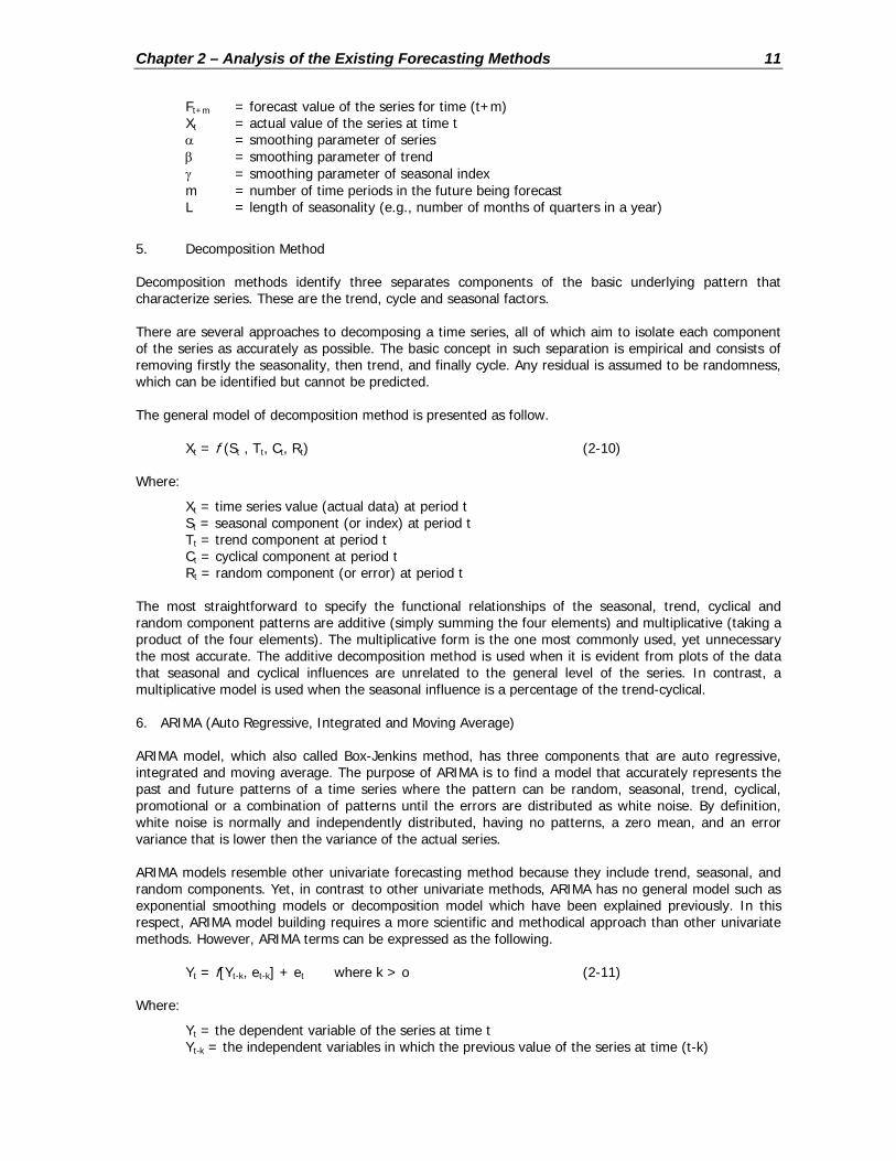
Chapter 2 – Analysis of the Existing Forecasting Methods 11
Ft+m = forecast value of the series for time (t+m) Xt = actual value of the series at time t α = smoothing parameter of series β = smoothing parameter of trend γ = smoothing parameter of seasonal index m = number of time periods in the future being forecast L = length of seasonality (e.g., number of months of quarters in a year)
5. Decomposition Method
Decomposition methods identify three separates components of the basic underlying pattern that characterize series. These are the trend, cycle and seasonal factors.
There are several approaches to decomposing a time series, all of which aim to isolate each component of the series as accurately as possible. The basic concept in such separation is empirical and consists of removing firstly the seasonality, then trend, and finally cycle. Any residual is assumed to be randomness, which can be identified but cannot be predicted.
The general model of decomposition method is presented as follow.
Xt = f (St , Tt, Ct, Rt) (2-10)
Where:
Xt = time series value (actual data) at period t St = seasonal component (or index) at period t Tt = trend component at period t Ct = cyclical component at period t Rt = random component (or error) at period t
The most straightforward to specify the functional relationships of the seasonal, trend, cyclical and random component patterns are additive (simply summing the four elements) and multiplicative (taking a product of the four elements). The multiplicative form is the one most commonly used, yet unnecessary the most accurate. The additive decomposition method is used when it is evident from plots of the data that seasonal and cyclical influences are unrelated to the general level of the series. In contrast, a multiplicative model is used when the seasonal influence is a percentage of the trend-cyclical.
6. ARIMA (Auto Regressive, Integrated and Moving Average)
ARIMA model, which also called Box-Jenkins method, has three components that are auto regressive, integrated and moving average. The purpose of ARIMA is to find a model that accurately represents the past and future patterns of a time series where the pattern can be random, seasonal, trend, cyclical, promotional or a combination of patterns until the errors are distributed as white noise. By definition, white noise is normally and independently distributed, having no patterns, a zero mean, and an error variance that is lower then the variance of the actual series.
ARIMA models resemble other univariate forecasting method because they include trend, seasonal, and random components. Yet, in contrast to other univariate methods, ARIMA has no general model such as exponential smoothing models or decomposition model which have been explained previously. In this respect, ARIMA model building requires a more scientific and methodical approach than other univariate methods. However, ARIMA terms can be expressed as the following.
Yt = f[Yt-k, et-k] + et where k > o (2-11)
Where:
Yt = the dependent variable of the series at time t Yt-k = the independent variables in which the previous value of the series at time (t-k)

Chapter 2 – Analysis of the Existing Forecasting Methods 12
et-k = The past error values between the forecast and actual at time (t-k) et = the error or residual term that represents random disturbances that cannot be explained by
the model.
In building ARIMA model, one should follow four steps, which are (1) identify the model by using graphs, statistics, transformation, etc., (2) estimate the parameter or determine the model coefficients, (3) diagnostic the model using graphs, statistics, residuals, etc., and (4) verified the forecast.
There are three ARIMA processes accordingly to the meaning of ARIMA itself. The first process is to build an Auto Regressive model, the second process is to build a Moving Average model and the third process is to build the Integrated model.
In determining each model of ARIMA processes, some identification tools are used which are the autocorrelation functions, partial autocorrelation functions, serial graph and descriptive statistics. Among those tools, a major identification and diagnostic tool of ARIMA analysis includes autocorrelation functions and partial autocorrelation functions. How these tools can identify ARIMA model will not be presented here.
Explanatory Methods
1. Simple Regression Model
This model predict the future by modeling the past relationships between a dependent variable and one or more other variables called either independent, predictor or exogenous variables.
In the simple regression model, the assumptions are a relationship exists between the variable that will be forecast and the basic relationship is linear. Thus, the dependent variable is a linear function of independent variable(s). The relationship is called linear because the increase (or decrease) in the independent variable brings proportional increase (or decrease) to the dependent variable.
The relationship of dependent variable (noted as Y) and the independent variable (noted as X) can be written mathematically when it is assumed to be linear as follow.
= a + bX (2-12)
is the estimated or forecast value for the dependent variable (Y). a is the point at which the straight line intersects the Y axis. The value of b is called the regression coefficient and indicates how much the value of changes when the value of X changes one unit. The most straightforward technique to calculate a and b is to plot the historical observations of Y and X. The most accurate model is that which yields a best fit line to the scatter plot and having the minimum sum of squared deviations between the actual and fitted values, hence this method is called method of least squared deviations.
To model a forecast using the simple regression model, the error or disturbances should be incorporated in the model, thus the regression equation will be:
Y = a + bX + e (2-13)
Where:
Y = the actual value of the dependent variable a = value of Y when X equals zero, called the Y-intercept b = slope, the change in Y resulting from a one-unit change in X e = residual error that remains after fitting the model
2. Multiple Regression
Y
Y
Y

Chapter 2 – Analysis of the Existing Forecasting Methods 13
In situation where more than a single independent variable is necessary to forecast accurately, a multiple regression should be done. With the assumption of linear relationships between the dependent variable and independent variables, the equation of multiple regression can be written as follows.
Y = a + b1X1 + b2X2 + …+ bnXn + e (2-14)
Where Y is the dependent variable, a is the value of Y when X1,...,Xn equal zero, b1,..,bn is the regression parameters, X1,…,Xn are the independent variables and e is the residual error that remains after fitting the model.
The goodness of fit (R2) is used to explain how each pair of variables is correlated. R2 is ratio of the explained variation over the total variation. A high value of R2, when data is sufficient and assumption of regression is satisfied, indicates that the relationship between variable does exist.
3. MARIMA (Multivariate Auto Regressive, Integration, Moving Average)
Pankratz (1991) has proved that a simple regression model is not sufficient to model a series which involves (1) time lagged relationship between the output and the inputs and (2) autocorrelation pattern of the disturbance series. This type of series should be modeled with a dynamic regression.
A dynamic regression is best to model a series with the characteristics as follows.
1. Involved time-lagged relationships; Yt may be related to Xt with a time lag, that is Yt may be related to Xt-1, Xt-2,… and so forth.
2. Involved feedback from output to inputs
Dynamic regression can be modeled using Multivariate ARIMA (Autoregressive, Integrated, Moving Average). In general, MARIMA models are combined univariate ARIMA and multivariate causal models having the attributes of both regression and ARIMA models- thus the term MARIMA, Multivariate ARIMA model The basic model of dynamic regression involved transfer function and noise model, thus the general model can be written as follows.
MARIMA = Transfer function + Noise model (2-15)
In order to develop dynamic regression, an ARIMA model should be priory developed for each variable for the following reasons:
1. ARIMA model built as the baseline model and set of forecasts.
2. ARIMA model presents the autocorrelation pattern very well.
3. To forecast with dynamic regression, the forecasts of the inputs are needed, thus ARIMA models that have been developed are used to forecast the inputs.
4. ARIMA model for stochastic inputs are needed to perform diagnostic checks of the dynamic regression model’s adequacy.
The ARIMA model has been explained previously in the time series method.
4. Econometric Model
The basic premise of econometric modeling is that everything in the real world depends on everything else while the major purpose of this model is to test and evaluate alternative policies and determine their influence on critical variables.

Chapter 2 – Analysis of the Existing Forecasting Methods 14
Econometric model is a model in which involves linear multiple regression equations, each including several interdependent variables. Structural equations are used to predict and explain the values of two or more dependent variables as functions of several other variables.
5. System Dynamics Model
System dynamics is the application of the principles and techniques of control systems to organizational and socio-economic problems. System dynamics model provides a presentation of the possible (future) behaviors of the complex and dynamic system. Thus, this approach is powerful when one should predict the future outcomes in which are the products of a complex and dynamic system.
System dynamic is defined as follow.
“System dynamic is a method to qualitatively describe, study and analyze complex system in terms of the process, information, organizational boundaries and strategies, which facilitates quantitative simulation modeling and analysis for the design of system structure and control …. The objective of system dynamic model is to clarify the relation between the behavior of a system as a function of time underlying processes” (Daalen, 2001).1
System dynamics are able to present the behavior due to its capability to model the structure of the system in which principally determine the behavior of this system. The structure not only contains the physical aspects, but also the policies imposed within the structure. This kind of structure involves delays and information feedback, which is one of the essential aspects within the system dynamics.
The general structure of system dynamics model consists of feedback; either positive feedback loop or negative feedback loop as presented in the following.
Figure 2-1. Positive and Negative Feedback Loop
The system dynamics model can be presented through a system dynamic diagram or ‘pipe’ diagram to represent system. The concept of system dynamic flow diagram are levels and rates. Level represents parts of the system in which accumulation occurs. Rates cause the value of level to change.
Lyneis (2000)2 presents that system dynamics models provide a means of understanding the caused of behavior, and thereby allow early detection of changes in the system structure and the determination of factors to which forecast behavior are significantly sensitive. In addition to that, system dynamics models allow the determination of reasonable scenarios as inputs to decisions and policies.
Advantages and Disadvantages of Models
The advantages and disadvantages of each model are presented in Table 2-1.
1 Daalen, E., W.A.H. Thissen, “ Dynamic Systems Modeling Continuous Models, System Dynamics”, TBM TUDelft, 2000. 2 Lyneis, James M., “System Dynamics for Market Forecasting and Structural Analysis”, System Dynamics Review Vol.16 No.1, John Wiley & Sons, Ltd., 2000
+
+ A
B
+
-
+ A
B
-

Chapter 2 – Analysis of the Existing Forecasting Methods 15
Table 2-1 Advantages and Disadvantages of Quantitative Forecasting Models
Forecasting Models Advantages Disadvantages
Double Moving Average
When trend and randomness are the only significant demand patterns, this is a useful method. Because it smoothes large random variations, it is less influenced by outliers.
In general, this method is too simplistic to be used by itself; it does not model the seasonality of the series. When using this method, one faces the problem of determining the optimal number of periods to use in the simple and double moving averages.
Brown’s Double Exponential Smoothing
Requires less data than moving average because one parameter is used, parameter optimization is simple.
Models the trends and level of a time series
Computationally more efficient than double moving averages
Loss of flexibility because the best smoothing constants for the level and trend may not be equal.
It is not a full model; it does not model the seasonality of a series, nevertheless many time series have seasonality.
Holt’s Two-Parameter Trend Model
Same advantages as Brown’s Double Exponential Smoothing
More flexible in that the level and trend can be smoothed with different weights
Requires two parameters to be estimated. Thus, the best combination of parameters is more complex than for a single parameter.
It does not model the seasonality of series.
Winter’s Three-Parameter Exponential Smoothing
It models trends, seasonality and randomness using an efficient exponential smoothing process.
The seasonal indexes are easily interpreted.
The parameters can be updated using computationally efficient algorithms.
The model’s forecasting equations are easily interpreted and understood by management.
Data requirements are greater than other methods within the exponential smoothing family.
This method might be too complex for data that do not have identifiable trends and seasonality.
The simultaneous determination of the optimal values of three smoothing parameters using Winters model may take more computational time than regression, classical decomposition or Fourier series analysis.
Decomposition Methods
Easily understood and applied. It provides user with an important
perspective on the underlying cause-and-effect relationships in a time series
It provides a very easy way of generating deseasonalized values.
Over-fitting models can be a problem due to the manner in which seasonal indexes and trends are calculated.
There may be a tendency to model large random variations as either seasonal or trend influences.
The division by abnormally low seasonal indexes might generate extremely large forecast.
It is very difficult to simultaneously decompose trend and seasonality in a series when only a few seasonal cycles exist.
Troublesome from a pure statistical point of view.

Chapter 2 – Analysis of the Existing Forecasting Methods 16
Forecasting Models Advantages Disadvantages
ARIMA (Auto Regressive, Integrated, Moving Average)
This model is powerful in describing all patterns involved in a series.
It is not an easy task to identify the combination of ARIMA components. This requires a statistical expertise and practices.
Simple Regression Model
Can be used to explain what happen to the dependent variable through changes in the independent variable.
It uses a statistical model to discover and measure and judge the validity of the relationship if one exists.
In order to forecast the dependent variable, the independent variable must be known, thus multiple forecast are needed to apply regression analysis.
Multiple Regression Model
It is an explanatory method that allows one to determine (estimate) virtually any kind of linear relationship that might exist between a dependent variable and one or more independent variables.
It requires estimates for the independent variables before forecast can be made.
A tendency of think that any time a high R2 (the coefficient of determination) exists, the regression equation is a good one. For this to be the case, the assumptions of regression must be satisfied and sufficient data must be available.
Econometric Model
Its ability to deal with interdependencies
Most powerful methods for measuring cause and effect.
The absence of a set of rules that can be applied across different situations.
MARIMA (Multivariate ARIMA)
Powerful to model when lagged independent variables affect the dependent variable.
Difficult to determine which subset of input variable results in the best model of the output variable.
The steps of identification, estimation, and diagnostic checking should be done interactively and iteratively, thus plenty of calculation should be performed.
When the transfer function is not dictated by the theory, then estimations of cross correlations or impulse response weights must be done to match these estimations against theoretical patterns.
General Remarks
The use of quantitative forecasting method gives general advantages and disadvantages that have been identified by DeLurgio (1998)3. The advantages are (1) less prone to biases, (2) can make efficient use of prior data, (3) reliable (given the same data, produce the same forecasting) and (4) optimal use of large volume of data. In contrary, the disadvantages are (1) myopic (knowing only about the data are
3 DeLurgio, Stephen A., “Forecasting Principles and Applications”, McGraw-Hill, 1998

Chapter 2 – Analysis of the Existing Forecasting Methods 17
presented to them), (2) slow to react to change, (3) need laborious process when a large number of forecast need to be made due to the requirement of removing all the noise of the past data before apply statistical methods, (4) managers who are well regarded for their knowledge of their products or markets may feel a loss of control and ownership if forecasts are delegated to a statistical model and (5) the processes underlying complex statistical models may not be transparent to forecast users and the outputs of these methods may be therefore attract skepticism. General characteristics of the typical applications of different methods are presented in Appendix A.
Qualitative Forecasting Methods
Introduction
Judgmental forecast is the most widely used approach of forecasting (Makridakis, 1989).4 It is preferable to perform for two reasons, which are (1) its ability to incorporate experts’ knowledge, and (2) it does not require personnel who are skilled in the use of statistical methods in which is a lacking resources in many organizations.
Judgment is involved in the forecasting problem in three aspects (Wright and Goodwin, 1998). First is the judgment about what data are relevant to the forecasting tasks. Second is the judgment of what forecasting approach to be used and the last is the judgment of the output of forecast when the forecasters using their domain knowledge to forecast.5
Besides its advantages, it should be noted that judgmental forecasting involves general pitfalls that have been identified by Amstrong (2001) which are (1) inconsistency and (2) bias.6 Inconsistency is a random or unsystematic deviation from the optimal forecast. It may arise because of variation in the way the forecasting problem is formulated, because of variation in the choice or application of a forecast method, or because the forecasting method itself introduces a random element into the forecast. Bias is defined as a systematic deviation from the optimal forecast. It may arise automatically when certain types of judgmental or statistical methods of forecasting are applied to particular types of data series.
Considering the fact that in any forecasting involves judgment (i.e., determination of the relevant data, forecasting technique to be used, etc), and considering the advantages of this method, it is important to explore the judgmental forecasting method besides the quantitative methods.
Choices Range
Judgmental forecasting is divided into two main methods, which are (1) the subjective forecasting method and (2) the exploratory forecasting method. The methods are presented below, and those are summarized from Makridakis & Wheelwright (1989), DeLurgio (1998) and Wright & Goodwin (1998).
The Subjective Forecasting Methods
1. The Jury of Executive Opinion
This technique consists of corporate executives, generally from sales, production, finance, purchasing and administrations, sitting around a table and deciding as a group what their best estimate is for the item to be forecast. Sometimes the executives are provided with background data or information that might be useful in assessing forecasts.
2. Sales Force Composite Methods
4 Makridakis, Spyros; Steven C. Wheelwright, “Forecasting Mehods for Management”, 5th edition, John Wiley&Sons, 1989, p. 240 5 Wright, George, Paul Goodwin, “Forecasting with Judgment”, John Wiley & Sons Ltd., 1998, p.272 6 Amstrong, J.Scott, “Principles of Forecasting, A Handbook for Researchers and Practitioners”, Kluwer Academic Publishers, 2001, p59

Chapter 2 – Analysis of the Existing Forecasting Methods 18
In this method, a forecast is obtained by collecting the forecast based on the views of individual sales people and sales management. It contains 3 different types, which are grass roots approach, the sales management technique and the distributor’s approach.
In the grass roots approach, the process begins with the collection of each salesperson’s estimate of probable future sales in his or her territory. Once the sales people have made their individual assessment, the results for the district forecast is put together.
The sales management technique is similar to grass roots approach, but the specialized knowledge of sales executive staff is used rather than assessments by individual sales persons. It could reduce the time required to obtain such forecast due to fewer people involved in the forecasting task.
The wholesaler or distributor approach is generally used by manufacturing which distribute their products through independent channels of distribution rather than through direct contact with the users of their products. It involves asking each of their distributors for the information about the size and quantity of the company’s product lines that they expect to sell in let say the next quarter of next year.
3. Anticipatory Surveys and Market Research-Based Assessment
The idea is to sample the population whose behavior and actions will determine future trends and activity levels of the items in question. Several surveys based on a sampling of intentions are prepared on a regular basis.
4. Subjective Probability Assessments
In this approach, an attempt is made to identify a range of values (the probability distribution) for the uncertain event. Only a finite number of outcomes of the variable are specified, and the judgmental assessment involves in determining the probabilities associated with each of these outcomes.
The Exploratory Forecasting Methods
1. Scenario Analysis
Scenario analysis is done to anticipate and influence future events in order to perform a more effective plan. In this method, alternatives future are predicted and the actions might be taken to support or modify these alternatives are identified.
2. Delphi Method
The Delphi method is the most formalized and studied of the structured group (Wright & Goodwin, 1998)7. This method is aimed to obtain the most reliable consensus of opinion of a group of experts by a series of intensive questionnaires interspersed with controlled opinion feedback.
3. Cross Impact Analysis
This method is used to estimate the effects of several related future events on the probability of another event. It formally defines the dependence of one or more forecasts on one or more other forecasts.
4. Analogy Methods
Forecast a product or technology that have characteristics similar to other products or technology. When sufficient data exists, the modeling analogies can be done using regression analysis and the concept of cross correlations. When sufficient data does not exist then subjective estimates are used.
Advantages and Disadvantages of Models
7 Wright, George, Paul Goodwin, “Forecasting with Judgment”, John Wiley & Sons Ltd., 1998,, p 206

Chapter 2 – Analysis of the Existing Forecasting Methods 19
Advantages and disadvantages of each method is presented in Table 2-2 which is summarized from Makridakis & Wheelwright (1989), Wright & Goodwin (1998), Thomas (1993) and DeLurgio (1998):
Table 2-2 Advantages and Disadvantages of Qualitative Forecasting Methods
Type of Forecasting Advantages Disadvantages Jury of Executive Opinion
Simplest method and most widely used
Provides forecast quickly and easily Does not require the preparation of
elaborate statistics Brings together a variety of
specialized viewpoints The only feasible means of
forecasting in the absence of adequate data or when substantial changes are taking place.
The weight assigned to each executive’s assessment will depend in a large part on the role and personality of that executive in the organization
Sometimes requires costly executives’ time
Disperses responsibility for accurate forecasting
Difficulties in making forecasting breakdowns by products, time periods, or markets for operating purposes.
Sales Force Composite Methods
Uses the specialized knowledge of those closest to the marketplace
Places responsibility for the forecasts in the hands of those who can most affect the actual results
Easy breakdown of the forecasts by territory, product, customer, or salesperson.
It is often that sales people are either overly optimistic of overly pessimistic
Sales people are unaware of broad economic patterns that may affect demand in their territory for various product lines.
Anticipatory Surveys and Market Research-Based Assessment
Helpful to prepare the estimation of market potential and market share for various products and services.
Need an expert to do the task; especially to determine and define the relationship among factors influenced the product sales.
Subjective Probability Assessments
Commonly used to incorporate individual judgment into forecasting.
Although individuals who know a lot about the variable to be forecast may have trouble making subjective probability assessments unless they are given a guidance as to how the assessments can be made.
Scenario Analysis Provide a framework to simplify and reduce the large number of possible events and factors and their relationships.
Very beneficial in planning when there is a great complexity in future uncertainties, the strategic plans of the past have lacked vision, previous long-range planning has been unsuccessful.
Able to consider many uncertainties at the same time.
Requires breadth of knowledge and imagination greater than that needed for the typical quantitative and other qualitative forecasting method.

Chapter 2 – Analysis of the Existing Forecasting Methods 20
Type of Forecasting Advantages Disadvantages Structured Groups (Delphi Technique)
Consensus is achieved where the variance in responses of Delphi panelists decreases over rounds.
Omitting bias due to experts from all over the globe can share ideas and conjectures.
Requires quite a long time to produce a forecast due to iterations structure required within the Delphi procedure.
Cross Impact Analysis Forces experts to consider the interactions of two or more technologies
Requires a very broad system of interrelationships.
Analogy Methods Very effective in modeling the expected seasonal demand for a new product that is either replacing an old one or that will have the same seasonal demand pattern as an established product.
Requires a selection of the analogous candidate in which not only comparable in one attribute but also in the whole situation.
General Remarks
After the presentation of the choices range and the advantages and disadvantages of each judgmental forecasting method, general remarks of the judgmental forecasting method are presented as follows.
1. The greatest advantage of the judgment forecasting which is not replaceable with the statistical quantitative method is its ability to incorporate expert’s knowledge. As a consequence, the use of judgmental forecast method should be emphasized on the intervention of expert’s knowledge to forecasting which cannot be incorporated by the quantitative method for example when there is less relevant numeric data.
2. Besides the general disadvantages of a judgmental forecasting which have been presented, one should bear in ones mind that human mind has a limited information processing capacity, thus the scope to which the judgmental forecasting task will be performed should be carefully determined.
3. Likewise in the quantitative method which has two main categories namely time series and explanatory, the qualitative method also has two main method categories which are subjective estimates and exploratory. The subjective estimates are procedures to obtain a forecast output through subjective estimation, while exploratory methods are structured procedures for exploring alternative futures. The selection of those methods should be harmonized with the objectives of performing a judgmental forecasting.
4. When selecting a judgmental forecasting method, one should aware not only the pitfalls of the particular method but also the possible general biases, thus arranging some attempts to reduce the risks is desirable. One alternative is by combining two or more methods.
Integration of Quantitative and Qualitative Forecasting Methods
Introduction
Realizing the general advantages and disadvantages of the quantitative and qualitative methods, an idea of integrating both methods was arising and this topic has been widely discussed. When a forecasting task is done with a pure judgmental method, problems may arise due to the biases and inconsistency characteristics involved in a judgmental forecasting. One might argue that a statistical method could result in a more reliable forecast, however Diamantopoulos & Winklhofer (2002) conclude that there is an

Chapter 2 – Analysis of the Existing Forecasting Methods 21
inconsistency in pinpointing the superiority of a particular type of forecasting technique toward accuracy.8 Moreover, a pure statistical method is perceived to be slow to react to change in a dynamic environment (Goodwin, 2001). This leads to a discussion on how an integration of a quantitative and qualitative method should be done to bring a complementary strength for an optimal forecasting process.
Integration Types & Procedures
Goodwin (2001) propose two types of integration, which are (1) the voluntary integration and (2) the mechanical integration. It is called a voluntary integration when the judgmental forecast is supplied with details of the statistical forecast and decides how to use this in forming a judgment. While, a mechanical integration is done through the application of a statistical method to the judgmental forecasting. The following will be discussed about each method and its procedure options in detail. The presentation of the methods is summarized from Wright & Goodwin (1998), Goodwin (2001) and Armstrong (2001).
Voluntary Integration
Procedures
There are two procedures to forming a voluntary integration of statistical method and judgment method proposed by Wright and Goodwin (1998). They are: (1) revising judgment and (2) revising extrapolations.9
1. Revised Judgmental Forecast
Experts make judgmental forecasts then it will be revised based on statistical extrapolations. The accuracy improves when the forecaster followed a structured procedure in which a preliminary forecast was made, the data were reviewed and the forecast was then revised.
A pitfall that has been identified is that the forecaster tends to put too much weight on their initial judgmental forecast when combining their judgment forecast with the statistical source (Wright and Goodwin, 1998).
Evidence suggests that the adjusted forecast would be superior if the time series adds information beyond what is in the judgments.
2. Revised Extrapolation Forecasts
A statistical forecast will be revised through a judgement of the forecaster(s) based on their domain knowledge. It is the most common way to integrate a statistical method and domain knowledge
The accuracy might improve if the forecaster is able to identify patterns that are missed by the statistical procedure and take advantage of causal information that the statistical method had not used.
Pitfalls of Voluntary Integration
General pitfalls of performing voluntary integration are identified as follows (Goodwin, 2001).
1. There is a danger of double counting bias. This can arise when a regression model is being used to produce the forecasts and a variable has been omitted from the model.
2. When the statistical method is reliably forecast part of the time series pattern and hence forming an ideal baseline for adjustment, people apparently ignore the statistical forecast completely.
8 Diamantopoulos, Adamantios; Heidi Winklhofer, “Export Sales Forecasting by UK Firms Technique Utilization and Impact on Forecast Accuracy”, Journal of Business Research, Elsevier, 2002 9 Wright, George, Paul Goodwin, “Forecasting with Judgment”, John Wiley & Sons Ltd., 1998, p.269

Chapter 2 – Analysis of the Existing Forecasting Methods 22
3. In many environments, judgmental adjustments are made on an ad hoc basis, without adequate documentation or a defensible rationale, so that the credibility of the forecasts to users may be damaged, and the opportunity to learn about and improve the role of judgmental intervention is lost.
Mechanical Integration
Procedures
Four procedures are proposed (Goodwin, 2001) for the mechanical integration, which are (1) combining, (2) bootstrapping, (3) correction for bias, and (4) correcting and combining.
1. Combining
Combined forecast is done by averaging the judgmental forecast and statistical forecast. A heavier weight would be given to the method that is perceived to produce a more accurate forecast. However, the alternative of attaching weights to the constituent forecasts and taking a weighted average can be problematical.
This procedure is more objective and enables to fully disclose the process of producing the forecast so that biases and political manipulation can be avoided.
One factor that influences the value of combining forecasts is the correlation between the errors of the forecasts in the combination. The combination is likely to be less effective when the correlation between the forecast errors is high because the second forecast is bringing little new information to the combination (for mathematics proof please refer to Goodwin, 2001)10. Indeed, the ideal situation is to have strong negative correlations between the forecast errors of the judgmental forecast and the statistical forecast, but this rarely found in practice.
2. Bootstrapping
Bootstrapping normally involves using multiple linear regression to build a model of a judge’s decision or forecasts. The usual form of the model is:
Ft = a + b1x1,t + b2x2,t + … +bnxn,t (2-16)
Where Ft is the judge’s forecast for period t, xn,t are the values of cues available to the judge at ‘t’, bn is the weight that the judge implicitly attaches to cue ‘n’, and ‘a’ is a constant.
The advantage of this method is that it average-out the inconsistency of human judgment. Meanwhile, there are two pitfalls identified. First is the difficulty in identification the cues due to a large number of possible cues that might be available to the judge. Second, the possibility that the judge has exclusive access to contextual information that cannot, by definition, be included in the model.
3. Correction for Bias
There are two methods of correction for bias, one is introduced by Theil and the other is introduced by Fildes.
The first form of correction for bias is the Theil’s correction. This method shows how the MSE (Mean Squared Error) of a set of forecasts can be decomposed to reveal two types of bias, mean and regression bias, plus a random bias. In the decomposition, the mean bias represents the tendency of the forecasts to be too high or too low. The regression bias represents a systematic failure of the forecasts to track the pattern in the actual. For example, a tendency for high forecasts to be too low and low forecasts to be too high. While, the random error is the variation in the actual that is not explained by the forecasts. By regressing the actuals to the forecasts then using the estimated actual at time t as the corrected forecast 10 Goodwin, Paul, “Integrating Management Judgment and Statistical Methods to Improve Short-term Forecasts”, Omega, The International Journal of Management Science, 2001

Chapter 2 – Analysis of the Existing Forecasting Methods 23
(for mathematics proof please refer to Goodwin, 2001), both mean and regression bias are removed from ‘past’ forecasts (i.e., forecasts where the actual has already been realized). Assuming that past biases will continue to be unchanged, the correction can be expected to remove systematic bias from future forecasts.
The second form of correction for bias is that the future forecasts are corrected by the predicted error. This involves regressing the forecaster’s errors on to the predicted variables. The Fildes’ method allows forecasts to be corrected for bias in the use of available information.
The third form is combine the Theil and Fildes models for correction. The problem of combination might be multicollinearity because of the relationship between the forecasts and cues.
4. Correcting and Combining
Given the propensity of judgmental forecasts to suffer from biases, it may be beneficial to apply correction to them before combining them with the statistical forecasts. This is a correct then combine strategy.
After the presentation of two types of integration, Goodwin (2001) gives a tentative decision tree to which conditions the implementation of each integration technique is desirable. This decision tree is presented in Figure 2-1.
Figure 2-2 Tentative Decision Tree of the Integration Method (adapted from Goodwin, 2001)11
11 Goodwin, Paul, “Integrating Management Judgment and Statistical Methods to Improve Short-term Forecasts”, Omega, The International Journal of Management Science, 2001
Series Type
regular withspecial eventsregular irregular
type of period
statisticalforecasting
correctedjudgmental
forecastnormal special
statisticalforecasting
availability of past'hard' data on special
ciscumstances
high low
statisticalforecasting
availability of data on pastjudgmental forecasts and
outcomes for specialperiods
high low
correctedcombine
likely impact ofspecial events
high low
voluntaryintegration
statisticalforecasting
Chapter 2 – Analysis of the Existing Forecasting Methods 24
Figure 2-2 depicts that there are three types of the data series, which are regular series, regular with special events and irregular series. Regular patterns or relationships favor the exclusive use of statistical forecasting. Irregular patterns, where each new observation in a series is a result of a combination of particular circumstances that apply only in that period, some of which the forecaster will have prior knowledge of (e.g., promotion campaigns), favor the use of judgment, albeit statistically corrected to remove biases. Most interesting are series that are a combination of regular patterns, overlaid with the effects of foreseeable special events. In periods when these events do not apply (‘normal’ periods), statistical forecasting is likely to be most accurate, as judgmental forecasters will be over influenced by the noise in the data. In ‘special’ periods, where there is a dearth of hard data on the special event, but ample past data on the performance of judgmental forecasts, a correct and combine strategy is likely to be most effective. In the absence of sufficient data to detect judgmental biases, voluntary integration should only be considered where the special event is likely to have a major effect on the variable to be forecast. Judgmental forecasters are not likely to be skilled in adjusting for minor effects as their judgments will again be distorted by the noise in the data. In this case statistical methods are likely to be most accurate even though they fail to take into account these relatively minor effects.
Principles of Integration
Wright and Goodwin (1998) propose some principles of integration as presented in the following.
1. Applying ‘no adjustment’ the default action, so that the judgmental forecast has explicitly to make request to adjust the statistical forecast, significantly reduced the number of harmful adjustments without reducing the propensity to make adjustments when they were appropriate. Harmful adjustments were reduced further when forecasters were also required to indicate a reason for requesting the adjustment.
2. Integration generally improves accuracy when the experts have domain knowledge and when significant trends are involved. Integration is valuable to the extent that judgments are used as inputs to the statistical methods, that they contain additional relevant information, and that the integration scheme is well structured. Integration harms accuracy when judgment is biased or its use is unstructured.
General Remarks
Integration of quantitative and qualitative method is done as an attempt to gain better accuracy under certain condition and to mitigate some of the behavioral objections to pure statistical forecasting, while also reducing the effects of judgmental biases. However, one should notice that when integration is incorrectly applied, it could harm accuracy.

25
Chapter 3. Formulation of the Forecasting Problem
Problem Outline
Decisions are the core of managerial processes in every business. In any decision-making situations, forecasting is an important input as the source of relevant information for making a decision. Yet, in a situation in which no information about the past performance exist likewise in a new business development case, predicting the future becomes a very difficult task. Therefore, a ‘good’ forecast as the input to business management process is desirable especially in a new business development.
As has been explained in Chapter 1, Unilever is developing a new business, thus a ‘good’ forecasting is inevitable. Many decisions should be taken accordingly in a large extent from marketing and sales strategy, financial planning, until supply chain operations in managing the new business development process. At this point, forecasting problem is not limited to the demand forecast but it has a broader meaning in accordance to the definition of forecasting given by Lyneis (2000). He defines forecast as a prediction, assumption, or viewpoint on some future event or condition, usually as a basis for taking action.12
One of the frequent forecasting problems which has been identified is the demand forecast. This is the driven factor in managing the inventory in accordance to the decoupling point between activities driven by forecasting and activities driven by order from customer. However, Forecasting problems may arise in the supply chain area when one should determine for instances how much product should be produced, how much inventory should be kept, how does the best practice of performing the distribution process and so on. It becomes very important in this case due to the short life span involved in the product being developed as discussed in Chapter 1.
In the next sub chapters, a detailed explanation about the problem specification and determination criteria of good forecasting will be presented.
Forecasting Functional Specification
The functional specification illustrates the users’ requirements of a forecasting model.
The first step in specifying the users’ requirements is to formulate the objective in the forecasting problem. The specifications, which are the lower level objectives, could be generated after the main objective is identified. In this study, the functional specification is specified by using an objective tree diagram approach as presented in Figure 3-1.
The main function of a forecasting is to give a good support in decision making. Good support to decision making can only be achieved when the forecasting yields a good result. Therefore, the main objective of this study from the forecasting user perspective is to have a good forecasting that supporting him/her in decision making situations. A good forecasting is determined to be a forecast which is (1) high in realization degree, (2) short preparation time, (3) high forecast adaptability, (4) high easiness using the method and (5) high confident on the result.
12 Lyneis, James M., “System Dynamics for Market Forecasting and Structural Analysis”, System Dynamics Review, John Wiley & Sons, Ltd., Vol. 16, No. 1, 2000

Chapter 3 – Formulation of the Forecasting Problem 26
Figure 3-1 Objective Tree of the Forecasting Process
The first attribute of a good forecasting is the ability of the forecasting process to yield a high realization degree of forecast. It means that the forecast should meet a certain level of accuracy and precision. Accuracy is defined as the ability of a measurement to match the actual value of the quantity being measured.13 In a forecasting case this definition implies that the forecast value should match to the actual value. The implication of this criterion to forecasting is that the forecasting model should be able to accurately describe future, thus the forecast result will be acceptable to be used as the information source in a decision making. Moreover, the forecast should also be precise, which means that the estimate results would not be vary much over different data set.14 A forecasting model could produce a high accuracy but low precision, low accuracy but high precision or even low accuracy and low precision forecast. However, what is expected is a forecasting model that could produce both high accuracy and precision forecast.
Secondly, the forecasting result should be available just before it is needed for a decision making. Considering the role of forecasting in a decision making, a high accurate and precise forecast becomes less valuable if it was presented after the decision was made. Therefore, the forecasting preparation time should be taken into account. A good forecast is the forecast that has short preparation time yet yields an appropriate result.
The third attribute is the ability of a forecasting process to adapt accordingly to a changing circumstances, for instances due to a changing in data pattern, and adaptive to out-of-sample data. This ability is determined by its adaptability, flexibility and extensibility capabilities. Adaptability describes the ability of a forecasting model to be modified accordingly to the changing in the circumstances, for instance when the forecasting process allows a procedure to re-estimate the parameters when new observations are available (Amstrong, 2001). Flexibility talks about the capability of a forecasting model to adapt to a certain range of extension, for example to the extension of the types of product. Adaptability is also determined by the degree of extensibility which means how far the forecasting model could be extended for instance when a new parameter should be added to the forecast model since new data are available.
13 “What is the difference between accuracy and precision”, Meteorologist Jeff Haby, http://www.theweatherprediction.com/habyhints/246/index.html 14 “Glossary of data mining terms”, Decision Craft Analytic, http://www.decisioncraft.com/datamining/glossary.htm
goodforecasting
highrealization
degree
highconfident on
result
high easinessusing themethod
shortforecastingpreparation
time
high easiness ofcomprehend the
model
great dataquantity
high forecastadaptability
highprecision
less datacorruption
highaccuracy
good datausedhigh flexibility high
extensibility
high easinessmodifying the
model
highinterpretability
good pastperformancein forecasting
good dataquality

Chapter 3 – Formulation of the Forecasting Problem 27
Finally, the users should confident in using the forecasting result. This confidence level is determined by four factors, which are the ease of comprehend, the ease of interpretability, the use of data and the past performance of forecasting. The ease of comprehend is important in order to prevent the risk of discounting the use of forecasting result by users simply because they do not understand the functions or relationships incorporated in the model. The ease of interpretability of the forecasting result is talking about how the result of the forecasting model should be interpreted, for examples interpreting the degree of relations, interpreting the cause and effect relations, or interpreting the model performance. Another criterion to achieve a high confidence level is a better data used. It could be achieved through the use of a great amount of good data which involves less data corruption. Last, when a model has proved to perform well in the past experiences, it will increase the users’ confidant to use the model.
From the discussion of functional specification, it can be seen that forecast accuracy is not the only important parameter in assessing a forecast method. In fact, there are still practical factors to be considered such as the easiness of using the method, the easiness of understanding the model, et cetera.
Forecasting Variable Specification
Forecasting System Diagram
In order to give a comprehensive understanding of the systems that are involved in the forecasting process within the company, a system diagram approached is used as presented in Figure 3-2. This diagram illustrates the system elements and defines the boundaries of the system in this study. It describes what are inside, what are outside the system and what are the expected results from the system.
Figure 3-2 Forecasting System Diagram
The demand, supply and inventory subsystem define the boundaries of the forecasting system which focuses in the supply chain area. In the forecasting process, demand, supply and inventory subsystems are influenced by some external factors, which are the marketing subsystem, the delivery subsystem and the production subsystem. The possible outcomes of interest of this system are forecast values of the sales, inventory and product availability in market.
Forecasting System
inventorysubsystem:- finished good fromproduction- existing stockavailability- safety stock
demandsubsystem:- retail and consumerdemand quantity
marketingsubsystem:- promotion type- channel type- geographic location- product growth- cost
supply subsystem:- distribution quantity- product availabilityin market
sales forecast(quantity)
delivery subsystem:- geographic location- transportation mode- cost- time
productionsubsystem:- productionthroughput time- raw materialavailability-production quantity
weather
inventory forecast(quantity)
productavailability
forecast (quantity)

Chapter 3 – Formulation of the Forecasting Problem 28
It can be seen from the diagram that a dynamic interaction between demand, supply and inventory subsystems within the forecasting system are present. For example, the attributes of demand subsystem influence the inventory and supply subsystems, while the inventory subsystem influences the supply subsystem. In addition, there are also influences from external factors to internal subsystems, for example from marketing subsystem to the demand subsystem. The complicated interactions between those attributes are not presented in this diagram since the intention is to help focus and identify the systems involved in the forecasting process. Nevertheless, the complete and complicated interactions of each attribute will be presented later in the causal relationship.
Forecasting Causal Relationship
Causal Relationships of Forecasting Process
One of the general principles structuring forecasting problem is to specify the causal chains involved in the forecasting process (Amstrong, 2001). 15 The causal chains might create feedback loops that could be used to identify the problems. In this case, a causal relationship diagram is used to specify the factors that have been identified in the system diagram and the relationships among them. Positive relation means that two factors have the same direction changes while negative relation means an opposite change direction. There is no hierarchical structure to develop a causal diagram. In this case, the development will be started with sales forecasting factor. The complete causal diagram of forecasting problem is presented in Figure 3-3. The factors in this diagram are marked with different colors accordingly to the subsystems in the forecasting system diagram to make it easier identifying the origin area of the factors. The dash circles point to the descriptive variables in which the direction of its relationship with other variable cannot be determined.
The actual sales for Unilever business are generated from the sales transactions between the company and its customers. Consequently, as illustrated in the causal diagram, the sales order forecast is influenced by the actual retail demand, the order fulfillment, the delivery lead-time and the promotion plan. All those factors give a positive influence in the sense that when the value of those factors increase then the sales forecast value will increase as well.
The retail demand is driven by the actual sales to consumer, the wholesaler price, the actual advertising and promotion campaign, especially promotion that is intended to the customers, the product growth factor, the percentage of ACV (All Commodity Volume) 16, the total market size and the product quality. All those factors give positive influences to the retail demand except the wholesaler price factor. The product growth factor is determined by the product position within its life cycle in which depends on the time factor. However, the relation between the production position within its life cycle and the product growth cannot be determined.
The actual advertising campaign is governed by the advertising campaign plan accordingly to the amount of budget that allocated for the advertising. When the advertising plan is executed to an actual advertising, an advertising cost will be generated which will reduce the budget allocation for advertising.
The actual sales to consumer is determined by the product availability in the market, the advertising activities such as TV commercial and actual promotion activities direct to consumer, the retail price, the population of targeted consumer, the weather condition, the percentage of ACV, the merchandising and placement of the product in the market. The last two variables are determined by the type of vending, but the relationship among them cannot be determined since the type of vending is a descriptive variable. All of those variables give a positive influence to the actual sales to consumer.
The percentage of ACV describes the penetration level of the products within its customers. It influences both the retail and consumer demand. When the willingness of the customers to sell the product across 15 Amstrong, J. Scott, “Principles of Forecasting, A Handbook for Researchers and Practitioners”, Kluwer Academic Publisher, 2001, p. 684 16 Percent ACV is a percentage of stores within the sample that sold at least one unit of an item weighted by the store's total dollar sales. Item Level Only. (SPIN Source, Help Manual, Measure Definitions, http://www.spins.com/help/measures.htm)

Chapter 3 – Formulation of the Forecasting Problem 29
their outlets increases, we may expect that the retail and the consumer demand will increase as well. This happens since an increase in percentage of ACV leads to the increase of the product availability in the market.
The actual sales to consumer will not only govern the retail demand, but also determine the market share and the product availability in the market. The more products sold to the consumers will reduce the product availability in the market. Here, the order fulfillment and delivery lead time are important to replace the sold products. It is possible that although the actual demand of the product is high, but since the order fulfillment level is low or the delivery lead time is too long, it creates a stock out condition and as a consequence results in a low actual sales to consumer.
Figure 3-3 Causal Diagram of Sales Order Forecast and the Loop of Interest (within the dashed lines)
Recall that the sales for the company is generated from the sales transaction between the company with its customers, thus the order fulfillment indirectly describes the sales achievement. When the company successfully fulfills an order from its customer, it means that the company succeeds in generating sales. The order fulfillment is determined by the availability of the products to be distributed, while this stock availability depends on the quantity of production.
The quantity of production is governed by the sales order forecast and the quantity of finished goods on hand. An increase in the sales order forecast will increase the production quantity, while a high quantity of finished goods on hand will reduce the production quantity.
actual salesto consumer
(unit)
sales orderforecast
(unit)
orderfulfillment
(unit)
retaildemand
(unit)
advertisingbudget
allocation(euro)
product quality-remaining timeto expiry date
(days)
productgrowth factor
(%)
productposition inlife cycle(binary)
wholesalerprice
(euro/unit)delivery
lead time(day)
productavailability
(unit)
productionthroughput
time(unit/day)
productionquantity
(unit)
+
+
+
stockavailability
(unit)
-
+
+
+
+
deliveryfrequency(times/day)
-
+
?
+
-
deliverydistance
(km)
+
-
retailerprice
(euro/unit)
+
-
promotionplan
(euro)
+
+
merchandising,space
allocation(m3)
+
placement(#outlet/
km2)
+
time+
vendingtype/format
(binary)
actualpromotion
(euro)
+
targetedconsumer(#people)
++
??
marketshare(%)
+
total marketsize
(euro)
+
advertisingcost
(euro)
+
weather(Celcius)
+
+
+
total cost(euro)
+
+
deliverycost
(euro/km)
+
+
+
+
% ACV (AllCommodity
Volume)
+
+
+
-
+
+
-
-

Chapter 3 – Formulation of the Forecasting Problem 30
The sales order forecast is also influenced by the delivery lead time. In principle, customers will take into account the required stock during the delivery lead time. The longer time takes to deliver the order to customer, the more volume required per order to provide stock during the lead time. The delivery lead time is influenced by the production throughput time, the delivery frequency and the delivery distance. When the production throughput time takes a longer time or the delivery distance is further, it will result in a longer delivery lead time. In contrary to that, when the delivery is done more frequently, it will reduce the delivery lead time.
At last, all those activities and processes that have explained generate costs when executed. The sum of those costs to some extent will affect the product price.
Identifying Loops
Several loops are constructed as presented in the causal diagram due to the complicated relationship between factors in forecasting process. Those loops are known as the feedback loops, which means one variable affects the other variables and vice versa, either directly or indirectly, through other variables.
The consequences of the influences may become clear quickly or after some time (van Daalen, 2000).17 Problems may arise due to the feedback loops, thus it is important to identify those loops to specify the forecasting problem situation.
The loops created in the causal diagram and the potential forecasting problems within each loop are described as follows.
Loop 1: Advertising budget allocation – advertising plan – actual promotion – advertising cost – advertising budget allocation
This loop consists of some decision factors correspond to the advertising or promotion. The factors involved in this loop are control factors because the company can determine the value of each factor. However, the uncertainty is involved in the advertising plan because the ‘effect degree’ of the actual promotion is unknown. A general proxy to measure the ‘effect degree’ of an advertising activity is the sales achievement.
Loop 2: Production quantity – stock availability – production quantity
The production quantity is one of the factors that should be determined by the company in its production planning. In determining the production quantity, the company should take into account the stock level at the projected time. A forecast problem arises since the stock figure in the future is uncertain. The company should perform a stock available forecast in order to make a decision in production planning.
Loop 3: Stock availability – order fulfillment – stock availability
The order fulfillment is another factor that should be determined by the company in its distribution planning. The order fulfillment is very much influenced by the availability of stock. While, the stock condition in the future is uncertain, thus creates a forecasting problem.
Loop4: Actual sales to consumer – product availability – actual sales to consumer
The actual sales to consumer is one of the important parameters of the product performance. The causal diagram illustrates that the actual sales to consumer will influence the retail demand, thus increase sales to the company. Hence, the company should maintain the availability of the product in the market by making a decision on how many products should be delivered to the market. This decision should take into account the existing product quantity in the market in the projected time in which the amount is uncertain. Therefore, a forecasting problem arises in predicting the product available in the market. In addition to that, the product available in the market is determined by the
17 Daalen, van E., dr.ir., Prof. Dr. W.A.H. Thissen, “Dynamic Systems Modeling Continuous Models, System Dynamics”, TBM Faculty, TU Delft, 2000

Chapter 3 – Formulation of the Forecasting Problem 31
actual sales to consumer, which is also uncertain. Consequently, a forecast of the actual sales to consumer might also be necessary to perform.
Loop 5: Sales order forecast – production quantity – stock availability – order fulfillment level – sales order forecast
In this loop, the factors that influence the decision of production quantity in the production planning are more elaborated. Besides determined by the stock availability in the projected time as explained previously, the production quantity is also determined by the sales order in the projected time. In fact, the prediction of sales orders quantity is essential in the production planning because the company’s target is emphasizing in the fulfillment of the sales order. Here the sales order forecast becomes the main factor while the stock condition will be the adjustment factor in the production quantity decision. Since the sales quantity in the future involves uncertainty, thus it arises a forecasting problem.
Loop 6: Sales order forecast – production quantity – stock availability - order fulfillment level – product availability – actual sales to consumer – retail demand – sales order forecast
A more extended factors involved in the company’s decision making situation is presented in this loop. Firstly, the decision of production quantity involves uncertainty since it is determined by the sales order and the stock availability in the projected time. As a consequence, it arises a forecasting problem. Secondly, the decision of order fulfillment or product delivered to the customer is determined by the sales order and adjusted with the product availability in the market. The product availability in the market is influenced by the actual sales to consumer as have been explained previously. The forecasting problem occurs in predicting the product availability in the market and the actual sales to consumer in the projected time.
After identifying the potential problems in forecasting as described above, the loop of interest is specified. In this case, the last loop is preferable to be examined in this study due to the following reasons. This loop identifies some forecasting problems in accordance to some important decisions within the supply chain issue that should be taken by the company, for instance the decision of production quantity and product delivery. The forecasting problems identified in this loop are corroborating with the potential outcomes of interest that have been specified in the system diagram. In addition to that, this loop takes into account factors from cross-area which are considerably important in accomplishing a forecasting task. This loop of interest is presented within the boundary at the causal relationship diagram in Figure 3-3.
Variables Specification
To develop a forecasting model, the variables that are going to be incorporated in the model should be determined. A forecasting model consists of variable(s) to be forecast namely the dependent variable(s) and influence variable(s) namely the independent variable(s). The dependent variables often involve uncertainty.
Notice that not all variables will be incorporated in the forecasting model. A judgment of the importance of the variable and the simplicity of the model is involved when specifying the forecasting variables. A variable classification helps modeler in specifying the variables for a forecast model. Table 3-1 presents the description of the variable classifications.
There are seven variables within the loop of interest, which are (1) the sales order forecast, (2) the production quantity, (3) the stock availability, (4) the order fulfillment level, (5) the product availability, (6) the actual sales to consumer and (7) the retail demand. The description and classification of those variables are presented in Table 3-2.

Chapter 3 – Formulation of the Forecasting Problem 32
Table 3-1 Variable Classifications
Substantial Nuisance
Control
This is a substantial variable in which under the company’s control and can be used as an instrument to influence the system. This variable is potentially incorporated in the forecasting model.
This is a variable in which under company’s control, but considering its low importance or relationship with the variable to be forecast, it might not be incorporated in the forecasting model.
Observed
This is a substantial variable in which can be observed but the company does not have power to influence this variable. Considering the substantial characteristic, this variable is also potentially incorporated in the forecasting model.
This is a variable in which beyond the company’s control yet observable. Considering its low importance or relationship with the variable to be forecast, this variable will not be incorporated in the forecast model.
Hidden
This is a substantial variable in which unobservable, thus the company cannot influence this variable. Considering its substantial characteristic, this variable might be incorporated in the forecasting model through a dummy variable.
This is a variable in which beyond the company’s control and unobservable. This variable is perceived to have low degree in influencing the variable to be forecast, thus it will not be incorporated in the forecast model.
Table 3-2 List of Variable for Forecasting Model
Variable Name Unit Variable Status Description
Sales Order Forecast Quantity Dependent & Substantial
This variable describes the prediction of sales order quantity in the projected time.
Production Quantity Quantity Independent, Controlled & Substantial
This variable describes the quantity of the finished good production. This is one of the decision variables incorporated in the production planning.
Stock availability Quantity Dependent, Observed & Substantial
This expresses the stock figure in the company’s finished good warehouse. It is very much influenced by the production quantity and the delivered product.
Order Fulfillment Quantity Independent, Controlled & Substantial
This variable is one of the parameters for measuring the service level. It presents the quantity of delivered product. This is one of the decision variables in the distribution planning.

Chapter 3 – Formulation of the Forecasting Problem 33
Variable Name Unit Variable Status Description
Product Availability in the Market Quantity Dependent &
Substantial
This variable describes the stock level in the market. This variable is not directly measured but could be predicted through some influence variables such as the sales order quantity, the order fulfillment level and the production quantity.
Retail Demand Quantity Independent, Observed & substantial
This variable presents the demand from retailer. It expressed as the actual order from retailer to the company.
Actual Sales to Consumer Quantity Dependent
This variable describes the consumer demand toward the product. This variable can be a hidden or an observed variable. If the company has information sharing agreement with its customer or if the company buys the data from a data syndicate, this variable becomes observed, otherwise a hidden variable.
From the table it can be seen that there are four dependent variables identified, thus four potential forecast problems exist. In this case, those variables will be analyzed to specify which dependent variables will be developed into forecasting models in this study.
Sales Order Forecast
The sales order forecast will be used in determining the production quantity in the production planning. This is one of the operational decisions that should be performed by the company in order to manage a good supply chain. Therefore, accomplishing a sales order forecasting task is essential.
Looking back to the causal diagram in Figure 3-3, the sales order forecast is influenced by the retail demand, the promotion plan, the order fulfillment level and the delivery lead time. The retail demand and the order fulfillment have been explained previously, thus the promotion plan and the delivery lead time will be explored further.
The promotion plan is a vague variable since the parameters to measure a promotion plan is unidentified. Fortunately, a proxy can be used as an approach to measure the promotion plan and its effect. The proposed proxies are (1) the amount of money budgeted for the promotion as the parameter for the promotion plan and (2) the sales achievement as the parameter of its effect. However, the relationship of the allocated budget with the sales achievement is not always linear, which means that the amount of money spent for a promotion or advertising is not a guarantee that it will influence the sales as expected. As a consequence, since the measurement of the promotion plan is hardly to identify, this variable will be incorporated in the forecasting model if it is perceived as an important variable, otherwise it will be treated as a nuisance variable.
The delivery lead time presents the time needed for the company to deliver the product to the customer. It is measured from the time when the company receives the order until the product is delivered to the customer. In fact, the delivery lead time does not involve a big fluctuation (the company commits to deliver within 1 to 2 days), thus the delivery lead time will not be incorporated in the forecasting model.
The function below describes the general relationship between the sales order forecast and its independent variables. This requires the parameters and the type of relationship should be specified further in a forecasting model.
Chapter 3 – Formulation of the Forecasting Problem 34
Sales order forecast = f (retail demand, order fulfillment level, promotion plan)
This notation tells that the sales order forecast is a function of the retail demand, the order fulfillment level and the promotion plan.
Stock Availability
The stock availability is determined by the production quantity and the order fulfillment. As explained previously, the production quantity is one of the decisions that should be taken by the company in performing its production planning and the product delivery is one the decisions in the distribution planning. The decision of product delivery is very much allied to the sales order forecast because product delivery is an attempt fulfilling the incoming orders from customers.
The function that would describe the general relationship between the stock availability as the dependent variable and its independent variables is as follow.
Stock availability = f (sales order forecast, production quantity, delivery quantity)
A prediction of the stock availability is very important to avoid an undesirable situation either excess stock or out of stock conditions. This situation could be anticipated when the company is able to predict what likely to happen in the future with the support of sales forecast information and the information of production and distribution planning. When something undesired happened, for instance on the production line, the company would be able to anticipate the effect of this situation to the stock availability by forecasting the stock condition so that the company would be able to take a proper decision to overcome the problem.
Product Availability in the Market
This variable is hardly to be measured directly unless the company develops information sharing with its customers. The prediction of the product availability in the market is useful to control the market’s stock in order to anticipate either stock out or excess stock condition in the market.
The causal diagram presents that the product availability in the market is directly influenced by the order fulfillment, the actual sales to consumer and the delivery lead time. Nevertheless, considering that the actual sales to consumer perhaps is an unobservable variable, thus the retail demand will be used to replace the actual sales to consumer based on an assumption that the demand from retail in such a way reflects the sales to consumer.
The function below presents the general relationship of product availability forecast.
Product availability = f (sales order forecast, production quantity, order fulfillment,
delivery lead time)
Actual Sales to Consumer
The causal diagram in Figure 3-3 presents that the actual sales to consumer is influenced by the weather condition, the placement of the product, the merchandising space, the population of the targeted consumer, the retail price, the actual promotion and the percentage of ACV. All of those influencing factors are the decision variables in which associated with the marketing and sales issue, for example a decision of what promotion should be done to increase sales to consumer, where the product should be placed to reach the targeted consumer, and so on. As a consequence, the problem arises from this variable is very much related with the marketing and sales department.
Yet, the actual sales to consumer forecast could have an implication in the supply chain problem. As presented in the causal diagram, the actual sales to consumer could be used as an approach to

Chapter 3 – Formulation of the Forecasting Problem 35
determine the retail demand. By doing so, it would reduce the risk of bullwhip effect (Chen et al, 1999)18 in the supply chain as the company performs the demand plan through the retail demand forecast. It is possible to be accomplished if the customers share their commercial information with the company. Currently, an attempt which leads to this possibility is being developed, for example by implementing the EPOS (Electronic Point-Of-Sales) system with its customer. Unfortunately not all Unilever’s customers are ready to run an information-sharing system, thus the complete figure of the actual sales to consumer is still hardly to acquire. As a consequence, it involves risk to develop a forecasting model using this data for the supply chain purpose.
General Remarks on Model Choices
In Chapter 2, a summary of the choices-range of the forecasting model has been presented to give a basic knowledge for developing a forecast model. In this chapter, general remarks of the model choices for each forecasting problem will be presented while further explanation of the model selection will be presented in the next following chapters accordingly.
In general, the function specification will always be taken into account when developing and determining the forecasting model for each forecasting problem.
Sales Order Forecast
The sales order forecasting problem in this case is associated with the production scheduling. In this case, being consider that manufacturing this type of product involves some fresh product materials, the ‘just in time’ concept is desirable for the inventory and production management. An accurate number is desired in determining the production schedule intended for managing the raw material as well as finished product inventory accordingly.
The intention in developing a forecasting model should be more emphasized on getting the most accurate forecast instead of getting an explanatory of the relationship between the sales order with its independent variables.
It has been presented in Chapter 2 that the time series method results in better predictive forecast compared to the explanatory or qualitative method. In the time series method, the underlying patterns in the series are predicted on the basis of historical data, thus independent from any decisions made on the identified decision variables.
In the sales order forecast problem, the existing historical data is the data of sales order in which expressed in the retail demand variable. The decision variables, which are the order fulfillment and the promotion plan, have been incorporated in such a way in the pattern of the series as long as no substantial changes involved in those two variables.
Another aspects that should be considered in choosing the forecasting model are the time horizon in which a decision will have an impact and the aggregate detail level in which a decision should be made. For the production scheduling purpose, the forecast should be applied in the immediate or short term decision horizon for an individual product or SKU level.
Therefore, the sales order forecast will be solved using a time series method due to the reasons that have been presented above. The method will be discussed in the next chapter.
Stock Availability Forecast
18 Bullwhip effect is an amplification effect of the increase of demand variability along a supply chain from retailers to distributors due to an increase in supply chain (Chen, Frank, Zvi Drezner, Jennifer K. Ryan, David Simchi-Levi, “The Bullwhip Effect: Managerial Insights on the Impact of Forecasting and Information on Variability in A Supply Chain”, Kluwer’s International Series of Quantitative Models for Supply Chain Management, 1999)

Chapter 3 – Formulation of the Forecasting Problem 36
The stock availability forecast is used to control the stock level in the inventory management. In a controlling process, one makes an influence attempt to the system being controlled in order to achieve the objective. The main concern in controlling process is the understanding to which an influence factor affects the output of the system. Hence the intention of the forecasting problem in controlling a system is to understand the predictable effect of each input factors to the output factor. This forecasting problem will be best modeled with an explanatory method.
In the explanatory method, any changes in the inputs affect the output in a predictable way, assuming the relationship is constant. The stock availability forecast implies that any decisions on the production quantity or the delivery quantity will affect the stock availability. In addition to that, to know the implication of the sales order forecast to the stock availability, this factor will be incorporated as an input factor.
Bear in mind that in a control process the effect of a decision involves time lags since any decision made at the current time will not affect the output immediately. This aspect is an important factor when selecting the forecasting model.
Multi inputs forecasting with time lags can be modeled with two approaches, one is the dynamic regression method and the other is the simulation method using the system dynamics model as presented in Chapter 2. The dynamic regression method is aimed to generate a specific forecasting model in which the relationships among the variables are mathematically modeled so the model can be used to forecast the dependent variable at its specific state. In contrary, the intention of developing a system dynamics model is to give an understanding of the behavior characteristics of the variables involved instead of determine the mathematics model of the interrelation between variables. Considering that the dynamic regression method determines the specific relation for each parameter, thus this method would be better performed in handling a few parameter since every changes in the parameters requires a lot of mathematical calculation. In addition to that, the dynamic regression method requires greater data to obtain a ‘good’ model compared to the system dynamics simulation approach.
Nevertheless, the purpose of developing the stock availability forecast is to predict the stock level in the projected time when a decision is made in a specific level. The stock availability forecast enables the decision-maker to take a corrective action when an undesired result occurred. Consequently, the dynamic regression method is preferable. In addition to that, the model only incorporates three parameters thus handling it with a mathematics calculation is not an issue.
As a conclusion, the stock availability forecast problem will be solved using dynamic regression method. A detailed discussion of this method will be presented in Chapter 5.
Product Availability Forecast
The product availability forecast is used to control the product availability in the market. The purpose of developing this model is to keep the product availability in the market in certain level to avoid either overstock or out of stock condition. In doing so, it is more practical to perform it in an aggregate level of product rather than in the SKU level for an aggregate vending-channel.
Likewise in the stock availability forecast problem, an explanatory method is preferable in performing the product availability forecasting. There are two approaches applied to model the product availability forecast, firstly a quantitative statistical method and secondly a system dynamics method.
The availability of the product in the market is resulted from a complex system. It involves causal relationships of processes in the supply chain. It is very much influenced by the actual sales to consumer and a sequential complex supply processes as described in the causal diagram. Modeling this forecast problem with a quantitative statistical method will need a plentiful of mathematics calculations. Besides, the aim of developing this forecasting is to understand the behavior of the system due to a policy imposed either in the decision variable or in the structural changes of the supply chain process. This leads to the choice of using a system dynamics approach with a simulation instead of a quantitative statistical method. This method will be discussed in Chapter 6.

Chapter 3 – Formulation of the Forecasting Problem 37
To conclude, three forecasting problems are identified, which are the sales order forecasting, stock availability and product availability in the market. The sales order is more suitable to be forecast using a time series model instead of explanatory model. The model should be able to handle the item level and be accurate to forecast a short-term forecast horizon. The stock availability will be forecast using an explanatory method. It is desirable since it would be used to control the inventory, so that the control variables should be incorporated in the model to understand their influence to the stock availability. The model should able to handle a time lag which is always involved in a control system. While, the product availability in the market forecast will be handled using the system dynamics approach. All of those methods will be more elaborated in the next three chapters.

38
Chapter 4. Sales Forecasting Model Using Winters’ Exponential Smoothing
4.1. Introduction
The sales order in this case will be forecast using a time series model namely the Winters’ Exponential Smoothing Method. This method involves three smoothing component operations to calculate the series, trends and seasonality influences.
The reason of choosing this method is classified into two main reasons. The first classification is related to the suitability of this method to be applied in the forecasting problem within the company. The second reason classification is related to the performance of this method compared to other forecasting methods which has been proved through some empirical studies.
The reasons with respect to the applicability of the method to be applied in the problem are relating to the characteristic and the typical applications (Appendix A) of the method compared to the forecasting problem in the company. Firstly, this method is able to model trend and seasonality patterns in data series. Seasonality pattern, such as due to weather conditions, and trends due to product growth are most likely consist in the sales data series of the chill product type. The explanation of these assumptions will be discussed later in the general requirement. Secondly, this method can be used for daily data and yields a high accurate forecast in the immediate forecasting horizon and applicable for production plan. These characteristics are relevant to the company’s forecasting problem in the following manner. One of the forecasting problems in the company is to forecast the sales order where the results will be applied in the production planning decision. Since the company is dealing with short life span products, the production should be planned and controlled in the daily basis. As a consequence, predicted values of the sales order per day for the projected times are essential. Thirdly, the number of observations required for performing this method is medium (24 – 48 data points) compared to other sophisticated method like ARIMA which requires more than 48 data points. This becomes one of the advantages of this method since the availability of the hard data of a new developing product may be limited.
Moreover, the chose of this method is supported by theoretical proof through empirical studies. Makridakis et al. in 1990 accomplished a comprehensive study of the accuracy of forecasting methods. They analyzed 1,001 different actual time series using 24 forecasting methods and 21 different forecasting methods for 111 series. This competition is now commonly called M-Competition. The 1,001 series varied by type (e.g., industry data, national data) and the time period analyzed (e.g., month, quarter, and year). The accuracy of each method is measured using five different statistical measures, and the methods are ranked based on their accuracy result. The result of the M-competition can be seen in Appendix B. From the result of the M-Competitions, it can be seen that Winters’ Exponential Smoothing performed well both in 1,001 series (average rank is 9.96) and in 111 series (average rank = 11.26). Moreover, it outperforms Box-Jenkins method (average rank = 11.53) in 111 series. Winters’ Exponential Smoothing performs less good than Lewandowski (average rank = 10.87) and Parzen (average rank = 11.22) methods in 111 series. Yet, it can be concluded from this study that there is no practical difference of the accuracy between the Winters’ Exponential Smoothing and the most sophisticated methods such as Lewandowski, Parzen and Box-Jenkins. This study indicates that the Winters’ Exponential Smoothing is a good forecasting technique.
Recall the functional specification that has been specified in Chapter 3, a trade off between the complexity and the accuracy of the model does exist. Higher accuracy is desired in order to achieve high realization degree of forecasting, while more ‘user friendly’, high understanding of the model and high interpretation of the model reflect that the less complex model is desired. Considering of this trade-offs, a judgment should be made for the chosen model. However, it is sensible to choose the simpler model

Chapter 4 – Sales Forecasting Model Using Winters’ Exponential Smoothing 39
when the accuracy is not significantly different and the applicability of the model to the problem is satisfied. This leads to the chosen of Winters’ Exponential Smoothing.
4.2. General Requirements
The general requirements for forecasting the sales order with respect to the following aspects are:
1. Horizon Length and Accuracy:
The model should accurately predict for immediate forecast. This means that the model should result in an acceptable accuracy when it is used to forecast the sales order for immediate time horizon. This is desired since the forecast will be used for the daily production scheduling. Looking back to the current forecasting practice in the company, the production scheduling is performed in the weekly basis. Thus, the model should accurately forecast the daily sales order in one-week time projected.
2. Data Period Used:
The model should be accurate in forecasting the daily data. As mentioned previously, this is required since the sales order forecast will be used for the daily production scheduling.
3. Aggregate Level:
The model should be able to forecast data in the SKU (Stock Keeping Unit) level. The sales order will be forecast in SKU level since the company should predict the demand of each SKU for the production planning. This also means that the model should be applicable when the company implements it for a great number of SKUs within the product category (the refrigerated prepared food product category).
4. Number of Observation Required:
The model should be applicable for dealing with relatively limited data. Since the product has just launched and still in the preliminary development stage, the data availability may be limited.
5. Pattern Recognition Capability:
The model should be able to recognize seasonality and trend pattern which is most likely consists in the sales data series. The underlying assumption of this requirement will be explained in the following.
Assumption of Seasonality and Trends Patterns Within the Series in the Case
Seasonality
Seasonal influences can be identified from a presented data. When the influences are recurrent and periodic, it identifies an existing seasonal pattern in the series. Seasonality exists due to two factors, which are external factors and internal operation factors.
The product studied in this case is prepared food products in which perceived consist seasonality pattern in its demand. The seasonality pattern in the sales of this product exists for two reasons, which are the way the company handle the supply operation and the external factor of weather as identified in the causal diagram in Chapter 3.
To understand of how the internal operation could influence a seasonality pattern in the sales data series, the sales order handling process should be understood which would be explained in the following.

Chapter 4 – Sales Forecasting Model Using Winters’ Exponential Smoothing 40
The company received incoming order from the customers everyday from Monday to Saturday. The delivery operation is also done from Monday to Saturday. Every incoming order which come before 3 pm will be delivered on the next day, meanwhile when the order comes after 3 pm will be delivered in the next 2 days. For example, if an order come in Monday before 3 pm, it will be delivered on Tuesday, while if it comes after 3 pm, it will be delivered on Wednesday. Assumed that in certain case, the products should available and accessible for the consumers for 7 x 24 hours is true for certain channels. This situation forces customers to place a greater order to satisfy the weekend’s demand where there is no delivery from the company. Since the customers desire to have the products on Saturday, thus they place the order either in Thursday afternoon or on Friday morning. Here, we can expect that the order will peak in those two days. Imagine when this pattern repeated every week, it creates seasonality pattern in the sales data series. This assumption should be proved by plotting the actual data series.
Besides the internal factors as explained above, the external factors would also generate seasonal patterns within the sales order data series. The external factor that has been identified is weather condition, yet other external factor such as holidays season might introduce seasonality in the sales data series.
The weather condition influences the sales of prepared food product, such as sandwich, when it is assumed that people like to enjoy a warm and good sunshine by doing some outdoor activities and they might buy a sandwich for their meals. This condition increases the sales quantity whenever a good weather is expected. Based on this assumption, the sales data series expected to increase in summer and decrease in winter. When this pattern repeated every year, it creates seasonality pattern in the sales data series.
However, as explained in the general requirements that the sales order forecast would be used for production scheduling in which leads to forecast the daily sales order, the daily influences should be incorporated in the model. As a consequence, the first assumption of seasonality pattern influence by the operational decisions is more applicable compared to the second assumption of weather condition in which more applicable for monthly or quarterly data.
Trends
Another type of pattern that expectedly exists in the sales order data series is trends. It describes the general increase or decrease in the sales quantity over time that lasts for some times. Trends are caused by many factors such as long-term population changes, growth during product, life style changes and so on. It is very sensible to expect an increase trends showed in the sales order data series considering that the product is in the developing phase of its self-life cycle. However, the data should prove whether a trend pattern consist in the series.
4.3. General Structure
The Formulae
The formulae of Winters’ Exponential Smoothing are as follows. These formulae are taken from the book of Forecasting Methods for Management (Makridakis and Wheelwright, 1989).19
St = ))(1( 11 −−−
+−+⎟⎟⎠
⎞⎜⎜⎝
⎛tt
Lt
t TSIX
αα (4-1)
Tt = 11 )1()( −− −+− ttt TSS ββ (4-2)
19 Makridakis, Spyros, Steven C. Wheelwright, “Forecasting Methods for Management”, 5th edition, John Willey & Sons, 1989, p. 80

Chapter 4 – Sales Forecasting Model Using Winters’ Exponential Smoothing 41
It = Ltt
t ISX
−−+⎟⎟⎠
⎞⎜⎜⎝
⎛)1( γγ (4-3)
Ft+m = (St + Ttm)It-L+m (4-4)
Where
S = smoothed value of deseasonalized series T = smoothed value of trend I = smoothed value of seasonal index F = forecast value X = actual value of the series α = smoothing parameter of series β = smoothing parameter of trend γ = smoothing parameter of seasonal index m = number of time periods in the future being forecast t = time L = length of seasonality (e.g., number of months of quarters in a year)
The basic idea of forecasting using the smoothing methods are based on the concept that when an underlying pattern exists in a data series, that pattern can be distinguished from randomness by smoothing (averaging) the data value. The effect of this smoothing is to eliminate randomness, so the pattern can be projected into the future and used to forecast.
The formulae consist of four equations, which are (1) smoothed value of deseasonalized series, (2) smoothed value of trend, (3) smoothed value of seasonal index and (4) forecast value. The meaning of each formula will be discussed further.
Smoothing Value of Seasonal Index (It)
To measure the seasonal component, a distinction of the patterns incorporated within the time series should be done. There are two general types of seasonal influences in the time series, an additive and a multiplicative. The Winters’ Exponential Smoothing model uses a multiplicative distinction to model the seasonality influences.
The seasonality index (4-3) within the Winters’ Exponential Smoothing model is used to interpret the seasonal influences within the time series. For example a seasonal index of 1.10 or 110% in period t denotes that the period is 10% higher than the trend-cyclical value.
To measure the seasonal component, the actual value of period t divided by the trend and cyclical components. In Winter’s model, the combined trend and cyclical components are expressed with the smoothed value of deseasonalized series (where the smoothed value of deseasonalized series will be discussed later), thus the seasonal index before smoothed is:
Ie = t
t
SX
(4-5)
Where I is the seasonal index, Xt is the actual value of the series at time t and St is the smoothed value of the deseasonalized series at time t, e is randomness.
The e in (4-5) denotes that the seasonality at each period is not perfect. It contains randomness. To eliminate the error and to isolate the seasonal indexes, the all of the computed combined seasonal error (Ie) should be averaged. As the underlying argument of exponential smoothing method is that the most recent observations contain the most current information about what will happen in the future should be given relatively more weight than the older observations, thus the seasonal index in Winters exponential smoothing will be smoothed to eliminate randomness. By ‘smoothing’ the seasonal indexes and giving

Chapter 4 – Sales Forecasting Model Using Winters’ Exponential Smoothing 42
weights of γ and (1-γ) to the most recent observation (4-5) and the old observation respectively (It-L) to decrease the value exponentially, the equation (4-3) is used to calculate the seasonal index at time t.
Smoothed value of Trend (Tt)
The second distinction is to distinguish the trend within the time series. Trend is an increase or decrease in a series that persists for an extended time. For non-seasonal data, many use a rule of thumb that a trend exists when seven or more observations show a consistent trend.
Based on the definition of a trend, a simple way to estimate trends is by calculating the difference between current actual value of series with the previous value. However, since the series is perceived to have a significant seasonality, thus the trends are calculated by subtracting the most recent value of smoothed deseasonalized series (the smoothed value of deseasonalized series at time t ) with the previous smoothed value of deseasonalized series (the smoothed value of deseasonalized series at time t-1). It can be written as the equation (4-7), where the smoothed value of deseasonalized series will be discussed later.
Tt = St – St-1 (4-6)
Likewise the seasonality index, the trends each period are not perfect. It contains randomness, thus the randomness should be eliminated. Using the same argument as used in the seasonality index, the trends value will be smoothed by giving different weights between the most recent trend value with the previous trend value. It results to the equation (4-2) to calculate the trends influences within the series with β and (1-β) as the weights for the most recent and the older value of smoothed deseasonalized series respectively.
Smoothed Value of Deseasonalized Series (St)
Since the method to distinguish the seasonality component has been developed successfully as explained previously, thus to calculate the overall level of the series, a deseasonalized series should be used. A deseasonalized series is a series in which the seasonal fluctuations have been eliminated from the actual value.20 Thus, what remains in this series is the pattern (in this case is trend). Recall to the multiplicative concept, deseasonalizing is done by dividing the actual value of the series with the seasonal index as presented in the following.
St = t
t
IX
(4-7)
St is the deseasonalized value of the series which incorporates the trend-cycle components at time t, Xt is the actual value of the series at time t and It is the seasonal index at time t. However, recall the equation (4-3), It cannot be calculated until the St is known. Therefore, the value of It-L is used as an approach in
attempting to calculate St. The first term in the equation (4-1) presents this calculation (Lt
t
IX
=
).
Yet, the value of the deseasonalized series should be smoothed by using the same concept of exponential smoothing in which the most recent value is given relatively more weight (α) than the old value to calculate St (the smoothed value of deseasonalized series at time t). Considering that the series contains a consistent trend, a single smoothing will create a natural lag (the value of St will trail behind that trend).21 Therefore, in order to eliminate the natural lag of single smoothing, the smoothed level (St-1) of period t-1 is adjusted by the trend (Tt-1) from that period.
20 Makridakis, Spyros, Steven C. Wheelwright, “Forecasting Methods for Management”, 5th edition, John Wiley &Sons, 1989, p.81 21 ibid., p.76

Chapter 4 – Sales Forecasting Model Using Winters’ Exponential Smoothing 43
Conclusion of Model Interpretation
From the equations (4-1), the most recent actual value of the series (Xt) is deseasonalized by dividing it with It-L. This is done to eliminate the seasonal fluctuation in the series. Then, the most recent trend available (Tt-1) is added to the previous smoothed value prior to smoothing in order to eliminate the natural lag. Thus, St in equation (4-1) is the trend-adjusted, deseasonalized level at the end of period t. Equation (4-2) estimates the trend by smoothing the difference between the smoothed values St and St-1. This estimates the incremental change (trend) in the level of Xt.
Initialization of the Starting Values
Considering the formulae that are going to use in this method, initial values are needed before this method can be applied to forecasting. There are several methods to initiate the initial values which are adopted from Makridakis and Wheelwright (1989)22 and deLurgio (1998).23
1. Least Square Estimates. Initial values can be calculated using ordinary least square. For instance, S and T can be found by solving the equation for a straight line to obtain the intercept and the slope, and using these as starting parameter values. While, the initial seasonal value can be estimated using the decomposition method, for example using the seasonal index and trend line from the percent of moving average method. Makridakis and Wheelwright (1989) claimed that this method is the most commonly used approach to initialization.
2. Backforecasting. Backforecasting is a commonly used method to make it appear that there are a larger number of observations in a data set. It involves inverting the data series and starting the estimation procedure from the latest (most recent) value and finishing with the first (oldest) value. This will provide forecasts or parameter estimates for the beginning of the data, and these can be used as initial values when the data are forecast in the usual sequence, that is, from the oldest to the most recent. DeLurgio (1998) said that backforecasting is an effective method that can be applied in many forecasting situations. It is easily implemented and effectively used.24
3. When only Limited Data Exist. When only a very few data exist, user might not think it is important to start with precise initial values. In such cases models that do not require starting values may be attractive. For example, the following initialization might suffice:
S1 = X’1 (4-8)
T1 = X’2 – X’1 (4-9)
e1 = 0
where X’1 and X’2 are deseasonalized values of X1 and X2.
In this case, if there are sufficient data (for example 3 times the seasonal period), the initialization of starting values will be calculated using the Least Square Estimates. Otherwise, the initialization will be calculated using most rough approach, which is the only limited data exist.
Ongoing Use of the Model
After initializing the model, Winter’s Method is used as follows.
1. At the end of period t, the actual series value (Xt) is recorded.
22 Makridakis, Spyros, Steven C. Wheelwright, “Forecasting Methods for Management”, 5th edition, John Wiley & Sons, 1989, p. 93 23 DeLurgio, Stephen A., “Forecasting Principles and Applications”, International Edition, Irwin McGraw-Hill, 1998, p.228-229 24 ibid., p.229

Chapter 4 – Sales Forecasting Model Using Winters’ Exponential Smoothing 44
2. Apply this value in equation (4-1) to calculate the smoothed value at time t. Note that all values in equation (4-1) are known at this time since the initial value has been determined.
3. Calculate the new trend of the sales order (Tt) by using equation (4-2).
4. Next calculate the newest value of the seasonal index (It) by using equation (4-3). Then adjust this and previous indexes so that they sum to the number of periods per year or season. These values will be used in the next forecast cycle.
5. Forecast future value of the series using equation (4-4).
Measuring Errors
Statistical analysis will be used to measure the forecast errors, the difference between the forecast value and the actual value. The common statistical methods to measure forecast error (forecast accuracy) are Mean Error (ME), Mean Absolute Deviation (MAD), Mean Squared Error (MSE), Percentage Error (PE), Mean Percentage Error (MPE), Mean Absolute Percent Error (MAPE) and Residual Squared Error (RSE).25 The formulae to measure forecasting accuracy are presented as follows.
Mean Error (ME) denotes the average of the deviations.
(4-14)
where e is the error and n is the number of observations. The drawback of measuring error using this method is due to the positive and negative deviations obscure the value of the deviations when they are averaged. However, this method is a useful measure of systematic error which is called bias. Bias is a consistent over- or under-forecasting that creates large cumulative errors.
Mean Absolute Deviation (MAD) denotes the average of the absolute errors. The formula of MAD is as follow.
(4-15)
where e is the error and n is the number of observations. This calculation is preferred compared to the Mean Error since it calculates the absolute value of the errors so that it does not obscure the deviations.
Mean Squared Error (MSE)
(4-16)
where e is the error and n is the number of observations. This method penalizes a forecast much more for extreme deviations than it does for small ones. Therefore, adopting the criterion of minimizing the mean squared error implies that several small deviations from the forecast value are favored than one large deviation.
Percentage Error (PE) measures the ratio of the error to actual.
(4-17)
25 DeLurgio, Stephen A., “Forecasting Principles and Applications”, International Edition, Irwin McGraw-Hill, 1998, p.37
n
eMAD
n
ii∑
== 1
∑=
=n
i
i
ne
ME1
n
eMSE
n
ii∑
== 1
2
)100(t
ttt X
FXPE
−=

Chapter 4 – Sales Forecasting Model Using Winters’ Exponential Smoothing 45
where Xt is the actual value at point t and Ft is the forecast value correspondingly.
Mean Percentage Error (MPE) measures the average ratio of the error to actual.
(4-18)
The MPE should typically be near zero as positive errors are offset by negative errors.
Mean Absolute Percentage Error (MAPE) measures the absolute of the average ratio of the error to actual.
(4-19)
In MAPE, the absolute values are used. Thus, positive and negative errors do not offset each other.
Residual Squared Error (RSE) is also called Standard Deviation of Errors or Standard Error of Estimate. It measures the dispersion of values about the mean error of zero.
(4-20)
This is used to generate prediction intervals about the mean error of zero.
4.4. Application of the Model in Unilever Case
Data
To calculate the sales order forecast using Winters’ Exponential Smoothing method, a set of appropriate historical data should be available. An appropriate data set means that the data used in the calculation should satisfy both the quantity and quality requirements. The data quantity simply points to the amount of data set used in the calculation. In this case, Winters’ Exponential Smoothing method requires at least 36 data points. While, the data quality has a broader meaning such as the data noise, level of aggregation, etc.
The data type has been specified in the general requirements of the sales order forecasting. To summarize, the data that needed to forecast the sales order is the historical data of daily sales order in quantity per SKU. The required data amount is at least 36 data points. For a daily data set, it equals to 36 working days of the actual sales order. The most current observations are supposed to describe the most current patterns involved in the data series. Consequently, an up to date data set is required.
The data set is gathered from a database which records the quantity of the actual sales order per SKU in the daily basis. Before the data is used for calculating the forecast, the data should be checked of the existence of outliers to avoid misrepresentations in the data. Outliers are the very large or small observations that are not indicative of repeating past or future patterns. Outliers include deviations that occur because of unusual events such as supply interruptions, strikes, plant shutdowns, competitors’ out of stock, or in contrary, competitors’ promotional campaigns, etc. However, in many cases, the cause of outliers may be unknown. These outliers should be removed from the series prior to forecasting.
To detect ouliers, two methods can be used, which are statistical test and judgment. In judgment, some tools, for instances an original data plot, an appropriate transformation, differences, or seasonal graphs might be necessary. In addition, the outliers can also be detected by performing statistical test. This is
n
PEMPE
n
ii∑
== 1
n
PEMAPE
n
ii∑
== 1
1
2
−= ∑
ne
RSE i

Chapter 4 – Sales Forecasting Model Using Winters’ Exponential Smoothing 46
done through measuring each observation as a standardized deviation from its mean and then performing a simple z- or t-test by using the following formula.
(4-21)
where:
t = t-value of each observation, Yt = Mean of Yt Sy = standard deviation of the observation
To adjust the outliers, there are some options could be done. If a reliable forecast exists for a series, an outlier can be replaced with the forecast value. Another options are to replace the outlier with the mean of the series if the series is completely random. While, when the series are autocorrelated due to a random walk or trend, the outlier can be replaced with the mean of the two adjacent values. However, if the series are autocorrelated due to a seasonality factor, the outlier should be replaced with the mean of the two seasonality adjacent values.
Calculation
Unfortunately, a calculation using the real company’s data set cannot be performed in this report due to data unavailability. This situation occurs due to the company’s confidentiality policy and the internal barrier in the cross-functions business interrelationships within the company’s environment. This will be discussed further in the end of the report.
However, the formulae and steps to calculate a forecast using Winters’ Exponential Smoothing method will be presented with the help of an example from a literature.
The Formulae
St = ))(1( 11 −−−
+−+⎟⎟⎠
⎞⎜⎜⎝
⎛tt
Lt
t TSIX
αα (4-21)
Tt = 11 )1()( −− −+− ttt TSS ββ (4-22)
It = Ltt
t ISX
−−+⎟⎟⎠
⎞⎜⎜⎝
⎛)1( γγ (4-23)
Ft+m = (St + Ttm)It-L+m (4-24)
Where
S = smoothed value of the deseasonalized series of the daily sales order (quantity/day) T = smoothed value of the trend the quantity of sales order (quantity/day) I = smoothed value of seasonal index F = forecast value (quantity/day) X = actual value of the series of daily sales (quantity/day) α = smoothing parameter of series (constant) β = smoothing parameter of trend (constant) γ = smoothing parameter of seasonal index (constant) m = number of time periods in the future being forecast t = time (day)
y
tt
SYY
t−
=
tY

Chapter 4 – Sales Forecasting Model Using Winters’ Exponential Smoothing 47
L = length of seasonality (constant = 6 days)
Steps to Forecast the Sales Order Using Winters’ Exponential Smoothing Model
Firstly, plot the series to identify whether outliers exist in the series. A statistical test as explained in equation (4-21) to detect outliers could also be performed when necessary. If the detection proofs that outliers exist, these outliers should be removed by replacing the values with new values which have been discussed previously. When the series are free from any outliers, this series is ready to be used in calculating the forecast.
Secondly, after the series is free from outliers, the initial value could be determined. Assumed that the data is sufficient for performing the least square estimates for initialization, thus this method will be discussed further as follows.
1. Assuming only n observations were available to estimate Tt, St, and It. Let say, n = 12 (2 weeks observations).
2. The differences in the value of the series over six 6-days periods accordingly to the seasonality periods are summed and divided by 36 (6 weeks x 6 days/week) to get an average daily trend value. For example:
36)(...)()( 6122817 XXXXXX −++−+−
= average daily trend value
3. Calculate the average value of the first 6 days (during the first week)
6... 621 XXX +++
= average value of the first week
This value becomes a base upon which St and Tt are projected. This value is centered on the period 3.5 [(6+1)/2].
4. To get the St + Tt values for any particular day, use the appropriate multiplier on the trend value of the average daily trend value that has been calculated in step (2). For example:
S1 + T1 = average value of the first week – 2.5 (average daily trend value)
S4 + T4 = average value of the first week + 0.5 (average daily trend value)
And so on
5. Calculate the initial seasonal factors by dividing the actual values for periods 1 to 6 by their respective St + Tt.
I1 = 11
1
TSX+
; I2 = 22
2
TSX+
; and so on
6. St for day-6 (assumed as the initial value of St) is obtained by divided the observed value for that period (X6) by the estimated seasonal index for that period (I6).
7. Use the average estimated trend that has been calculated earlier for the initial value of trend at period 6 (T6).
8. Fitted value for the next 24 periods (period 13-period 36) were used to determine values of α, β and γ that minimize the sum of the squared errors.

Chapter 4 – Sales Forecasting Model Using Winters’ Exponential Smoothing 48
When the initial parameters have been determined, the Winters’ Exponential Smoothing model could be further used to forecast the future sales by using the equations 4-21 until 4-24 that have been presented earlier. Continuing the above calculation of the initial value, once the actual value of period 36 is ready, this value is used to calculate the smoothed value of period 37 by using equation 4-21. Then, calculate the new trend of period 37 using equation 4-22 and also calculate the seasonal index of period 37 by using equation 4-23. To forecast, use equation 4-24 and inputting the smoothed value, trend and seasonality index values that have been determined.
To make the above steps better understood, an example from a literature will be presented in the next box. This case is adopted from DeLurgio (1998) as an attempt to understand the Winters’ Exponential Smoothing. The complete calculation can be seen in Appendix F.
Case Example: (Adopted from DeLurgio, 1998, p.224-230) A set of a data series is presented in Appendix F1. Assumed that it is a monthly sales data of a product. From the plot of the data which is presented in Appendix F2, it can be seen that there are no outliers expected and also the series pattern indicates the involvement of seasonality of a year period. 1. Initialization of the Starting Value
Assumption: only 15 observations (X1 to X15) were available to estimate initial values of Tt, St and It. The differences in the value of the series over three 12-months periods are summed and then divided by 36 to get an
average monthly trend value.
36)()()( 315214113 XXXXXX −+−+− = average trend (3 years) (ex-1)
917.736
)660729()578711()546629(=
−+−+−
The average value of the first 12 periods becomes a base upon which St and Tt are projected (column 5).
12... 1221 XXX +++ = average value of the first year (ex-2)
12604...578546 +++ = 696.50
This value is centered on the period 6.5 [(12+1)/2].
To get the St + Tt values (column 5) for any particular month, use the appropriate multiplier on the trend value of the average monthly trend value that has been calculated (7.917). For example:
St + Tt for period 1 = 696.50 – 5.5(7.917) = 652.958 (ex-3) St + Tt for period 2 = 696.50 – 4.5(7.917) = 660.875, and so on
Calculate the initial seasonal factors by dividing the actual values for periods 1 to 12 (column 2) with their respective St + Tt (column 5)
I1 =
11
1
TSX+
= 958.652
546 = 0.836 ; and so on (ex-4)
St (column 3) for month-12 (assumed as the initial value of St) is obtained by divided the observed value for that period (X12) by the estimated seasonal index for that period (I12).
S12 = 604/7.917 = 740.042 (ex-5)
Use the average estimated trend that has been calculated earlier (7.917) for the initial value of trend (column 4) at period 12 (Tt12).
Fitted value for the next 24 periods (period 13-period 36) were used to determine values of α, β and γ that minimize the sum of the squared errors. From the calculation, the optimum value of α is 0.33, β is 0.05 and γ is 0.75 with the sum of squared errors (RSE) is 50.2593
2. Forecasting
St = ))(1( 11 −−−
+−+⎟⎟⎠
⎞⎜⎜⎝
⎛tt
Lt
t TSIX
αα (ex-6)
S36 = 0.33 ))(33.01( 353524
36 TSIX
+−+⎟⎟⎠
⎞⎜⎜⎝
⎛ = 895.797

Chapter 4 – Sales Forecasting Model Using Winters’ Exponential Smoothing 49
Forecasting Result and Its Accuracy
The above example uses the minimum mean squared error (RSE) criterion or the standard deviation of the errors to determine the parameter values of α, β and γ. The RSE describes the deviations of the error from the mean of error. While, the mean of errors is expected to be zero.
The forecast accuracy is measured using the mean of absolute percentage error (MAPE). This term describes the forecast accuracy in the following manner. If the MAPE is 0, it means that the forecast is deviate 0%, thus 100% accurate. The example which presented in Appendix F shows that for the fitted value of the series, the MAPE value is 4.288. It means that in averages the forecast is deviates 4.288% from the original (actual) series value. Therefore, the accuracy of fitted series value is 95.712%. While, when the model is used for forecasting the in-sample series, the MAPE is increase to 5.795. This means that the forecast accuracy is decrease to the level of 94.205%.
The above example is used to forecast the monthly data series for 12-months or 1-year forecasts horizon. The result is quite satisfactory since the accuracy achieve around 94% - 95%, thus only 5% - 6% deviations from the actual series value in which either over- or under-forecast per period.
4.5. Final Remarks
A possible drawback selecting Winters Exponential Smoothing method to forecast the sales order is due to the theoretical reason resulting from the M-competition study. Although this method performed well when it was competed with other forecasting methods, it is still unclear on how close the data used in the M-competition corresponded to the company’s problem. However, it can be seen from the above example that the forecasting calculation using Winters Exponential Smoothing method is relatively simple. The are 3 parameters should be estimated, which are α, β an γ. These parameters could be calculated with the support of a spreadsheet software application or available forecasting software application. As a consequence, this method is suitable to be used for forecasting the daily sales order of the product in SKU (item) level for the production scheduling purpose. Therefore, it can be concluded that this method is potential in helping the company to achieve the objective of conducting the sales order forecast.
Supposed that the above example was applied for the daily sales order of the refrigerated prepared food product, the implications could be expected as follows.
The model was applied to forecast the sales order for the next 12-working-days, thus 2-weeks time horizon. The forecast accuracy for the whole 2 weeks was around 94% - 95%. Therefore, it could be expected that this model also work well for a shorter time horizon forecasting, for instance 1-week horizon as the current practice in the company for production scheduling purpose.
Tt = 11 )1()( −− −+− ttt TSS ββ (ex-7)
T36 = 0.05(S36 – S35) + (1-0.05)T35 = 6.586
It = Lt
t
t ISX
−−+⎟⎟⎠
⎞⎜⎜⎝
⎛)1( γγ (ex-8)
I36 = 24
36
36 )75.01(75.0 ISX
−+⎟⎟⎠
⎞⎜⎜⎝
⎛ = 0.894
Ft+m = (St + Ttm)It-L+m (ex-9)
F37 = (S37 + T37 (1))I25 = 785.842 F38 = (S38 + T38 (2))I26 = 831.484 …. F48 =(S48 + T48 (12))I36 = 869.003

Chapter 4 – Sales Forecasting Model Using Winters’ Exponential Smoothing 50
As a consequence of the forecast accuracy that has been explained previously, the expected absolute deviation is 5%- 6% per day. It means that the actual sales order might approximately 2.5% - 3% higher or below the forecast value. This would help the company in determining the production quantity that take into account the safety stock or buffer due to the error in forecast.
The model need to be modified for the seasonality period since the assumption of the seasonality period was 6-days instead of 12 periods likewise in the example.
Looking back to the assumption of the seasonality factors involved in the refrigerated prepared food products, this type of product is also presumed involving seasonality factors due to yearly seasons (i.e. winter, spring, summer and autumn) in addition to the daily internal operation. The application of the model which purposed in this case takes into account only the seasonality due to the daily internal operation. Consequently, the model might need to be revised, for instance in the beginning of every season, since the pattern of the data might be changed due to the season. The company should aware the possibility of big pattern changes occurred as the season is changed.
When performing forecast for the product SKU level, there is a possibility that some SKU might have zero sales orders, thus the series consists of many zero values. This would apply for example when dealing with a non-regular product or a very slow moving product. If the series consists of many zero values, a problem may arise, as this series cannot be used for estimating the pattern of the data. Thus, an action should be done to overcome this problem. In dealing with a very slow moving product, it seems that performing a forecast using Winters Exponential Smoothing method is not suitable. These slow moving products could be forecast using other methods, for example simply by a naïve method or judgmental method since the affect of this method to the service level is expected to be low. While, in dealing with a non-regular product, it is suggested performing the Winters Exponential Smoothing by treating these products as 1 SKU, for instance the promotion SKU or the variant SKU. This is explained as the following. Supposed the company has 5 fix SKUs (e.g. tuna, egg, chicken, ham and vegetarian sandwich) which are produced in the daily basis and also 1 variant SKU which is changed every week, for example, egg-tuna sandwich, egg-ham-cheese sandwich, etc. Those variants could be treated as 1 SKU, which is the variant SKU. By doing so, the sales order of these SKUs could be forecast using the Winters Exponential Smoothing method with the assumption that the demand for those variants are not significantly different.
To summarize, the Winters Exponential Smoothing Method is a relatively simple forecasting method that is suitable for forecasting the sales order in the daily basis for the product item level, thus can be used for production scheduling purpose. Revisions of the parameters might be necessary as the changes in the sales order patterns, for instance due to yearly seasons. This method is only suitable for regular products, or non-regular products that are treated as a regular product.

51
Chapter 5. Inventory Forecasting Using MARIMA (Multivariate Auto Regressive, Integrated, Moving Average) Model
Introduction
The second forecasting problem that has been identified in Chapter 3 is the stock availability forecasting. Prediction of stock availability is very important to avoid undesirable situations either excess stock or out of stock conditions. This situation could be anticipated when the company is able to predict what inventory condition is likely to happen in the future with the support of sales forecast information, production quantity and delivery fulfillment which has been specified in Chapter 3. For example, supposed that the company anticipates lacks of some raw materials to which limit the production quantity. The company would be able to anticipate the effect of this situation to the stock availability by forecast the stock condition so that the company would be able to take a proper decision to overcome the problem. This process involves feedforward control actions to the stock availability or inventory.
It is quite apparent that in a control process, feedback and delays are involved thus creates a dynamic system. In a dynamic system, it should be realized that when an action is taken time lags or delays would be involved between the action and its total effect in the system. The same concept applied to the inventory forecasting. An action with respect to, for instance, the production quantity will influence the stock availability and other factors involved with some delays times.
Looking back to Chapter 2, a dynamic system which involves delays characteristic can be forecasted through 2 model approaches, which are the dynamic regression with MARIMA (Multivariate Auto Regressive, Integrative, Moving Average) model and system dynamics with simulation approach. While, system dynamics approach has great advantage of its ability in modeling feedback besides delays. The choice between these two methods depends on the purpose of conducting the forecast. When the aim is to predict the outcome values of the stock availability, the mathematics model using dynamic regression is preferable. Meanwhile, when the objective of conducting the stock forecast is intended to understand the behavior of the stock level, the system dynamics modeling with simulation approach is favored.
In the Unilever case, considering that the intention of conducting the stock availability forecast is to control the output of stock level for its operational inventory management to avoid the undesired stock conditions of the perishable products, the MARIMA model should be selected rather than the system dynamics model. This MARIMA model would be used as a feedforward control tool. The company determines an inventory target and then the inventory forecasts would be compared to this target. When the forecast values show discrepancy with the target value, necessary actions could be taken.
General Requirements
General requirements for forecasting the stock availability with respect to the following aspects are:
1. Horizon Length and Accuracy:
The model should accurately predict the immediate to short term forecast. This means that the model should result in an acceptable accuracy when it is used to forecast the stock availability for immediate to short time horizon. This is desired since the forecast will be used for the daily operational stock control.
2. Data Period Used:

Chapter 5 – Inventory Forecasting Using MARIMA Model 52
The model should be accurate in forecasting the daily data. This is required since the stock availability forecast will be used for the daily operational stock control so that daily data will be used as the input of forecasts.
3. Aggregate Level:
The model should be able to forecast data in the product aggregate level, for instance in the product family level. The stock availability will be forecast in the aggregate product level since the inventory target for short life span products is ‘zero’ (as low as possible) inventory for all products so that it is unnecessary to confirm whether each item satisfies this target. Consequently, stock controlling process will be done in the aggregate product level instead of in SKU level.
4. Number of Observation Required:
The model should be applicable for dealing with relatively limited data. Since the product has just been launched and is still in the preliminary development stage, the data availability will be limited.
5. Pattern Recognition Capability:
The model should be able to explain the relationships between variables of stock availability with production quantity, sales order forecast and order delivery. It should also be able to cope with time lags as the control process characteristic. This is desired since the model is going to be used to predict the future stock availability due to for instance production quantity decisions in the production planning. The relationships of those variables will be explained in the following.
Causation
As explained in the general causal diagram in Chapter 3, the stock availability is influenced by the production quantity as the acquisition rate, while the stock availability will further affect the order fulfillment level. The later can be said that the stock availability is influenced by the delivered product quantity as the loss rate. One step further, the causal diagram says that the delivered quantity or order fulfillment is determined by the sales order or retail demand.
The developing of the statistical model is an attempt to know the relationship between the dependent variable Y, which is the stock availability (inventory level), and the dependent variables X which are the production quantity, the delivery fulfillment level (or the delivered quantity) and sales order quantity. The general statistical modeling to explain these relationships is the regression model.
Those variables are incorporated in the model due to two reasons. Firstly, those variables have causation relationship with stock availability according to the causal analysis that have been performed in Chapter 3. Secondly, they could be one of the causes of problem and also could be one of the control variables for the company in order to cope with either excess or out of stock conditions.
Besides being used to explain the relationship between dependent variable and independent variables, the regression model has other purposes in which to measure the degree of association (correlation) between those variables and to measure the error in using the relationship to predict the dependent variable.26
Time Lag
The above causation does not explain about the time lags involved in the process. However, consider a time lag is important since the output Y (prediction of stock availability) might not be related only to Xi,t
26 DeLurgio, Stephen A., “Forecasting Principles and Applications”, International Edition, Irwin McGraw-Hill, 1998, p. 96

Chapter 5 – Inventory Forecasting Using MARIMA Model 53
but also to Xi,t-1, Xi,t-2, and so on (Pankratz, 1991)27 and even with Y past value (Yt-k). For example, the stock availability is related to production quantity, but it is quite clear that the stock availability is not simply determined by the today’s production, but may also be determined by some previous day productions. Moreover, the current inventory level is also possibly influenced by its past values. As a consequence, the relationship involves time lags between the stock availability and the production quantity thus creates a complex and dynamic relation.
The appropriate way to determine the number of time lags that should be incorporated in the model is to include the longest time lagged response that might reasonably expected to be important. Next, the coefficient of the impulse of each independent variable with respect to time is calculated and then a tentative transfer function could be estimated by comparing the estimated impulse pattern with some common theoretical impulse function.
Assumptions could be made to judgmentally determine the possible time lags. For example, for the case of fresh food products, suppose that the life span of the product is 3 days, it is fairly sensible to include only 3 time lags for the production quantity variable because the products manufactured 4 days before are already expired. This also prevails with the sales order variable. For example, depending on the company’s target of the delivery lead time, the time lags between sales order and stock availability could be judgmentally determined. Suppose that the delivery lead time is 2 days and there is no backlog policy, thus the sales order today would be delivered by tomorrow or the day after. Then it could be expected that the time lag between sales order and stock availability to be 2 or 3. However, this causation involves several complexities, thus may result in a nonlinear relationship so that it is inappropriate to model it using a simple multiple regression. As a consequence, simply determine the time-lags by judgment should be avoided.
According to the above explanation, the generic model for describing the inventory level or stock availability is as follows.
Inventory level (t) = f [inventory level (t-k1), production quantity (t-k2),
delivery (t-k3), sales order (t-k4), error (t-k5)]
Regression models with time-lagged inputs are called ‘distributed lag’ models (Pankratz, 1991) 28 and it is best modeled using MARIMA model (DeLurgio, 1998). 29
General MARIMA Model
In this sub chapter, the general model of MARIMA and the theoretical functions to build the model are presented. Those are summarized from DeLurgio (1998), Makridakis (1989) and Pankratz (1991).
In general, MARIMA models are combined univariate ARIMA and multivariate causal models having the attributes of both regression and ARIMA models – thus the term MARIMA, Multivariate ARIMA models. This model is able to model the relationship between dependent variable and independent variables which involves several lags, both to the past values of the dependent variable itself as well as to the past value of independent variables.
In the inventory control problem, a dynamic relation is involved since the current inventory level is related either to the several past inventory quantities and/or to the several past production quantities, delivery quantities and sales order quantities as has been discussed.
The generic model of MARIMA is as follow. 27 Pankratz, Alan, “Forecasting with Dynamic Regression Models”, John Wiley & Sons Inc., 1991, p. 102 28 ibid., p. 147 29 DeLurgio, Stephen A., “Forecasting Principles and Applications”, International Edition, Irwin McGraw-Hill, 1998, p. 534

Chapter 5 – Inventory Forecasting Using MARIMA Model 54
MARIMA = Transfer Function + Noise model
For this case study, the model that would be developed is a model that is able to explain inventory level (Yt) as a function of X1,t, X2,t, and X3,t as presented below.
Yt = f(X1,t-k, X2,t-k, X3,t-k, Yt-k) + Nt (5-1)
Where:
Yt = inventory level at time t (quantity/day) X1, t-k = production quantity at time [t-k] (quantity/day) X2, t-k = delivery quantity at time [t-k] (quantity/day) X3, t-k = sales order at time [t-k] (quantity/day) Yt-k = past value of inventory level at time [t-k] (quantity/day) Nt = regression disturbances (noise model) at time t k = time lags
DeLurgio (1998) gives a guidance to identify, estimate and diagnose the above relationship in the following way.30
1. Develop an ARIMA model of the output (Yt); this becomes a benchmark for judging the fit of the multiple input MARIMA model as well as a potential noise model.
2. Develop an ARIMA model for each input variable (Xi,t) in order to prewhiten it and to pretreat the output variable (Yt). Prewhiten and pretreat will be discussed later.
3. Develop a MARIMA model explaining output variable (Yt) as a function of each input variable (Xi,t-k) and noise model (Ni).
4. Develop a three input MARIMA model explaining output variable (Yt) as a function of input variables (Xi,t-k), and noise model (Nt). The fitted one-input MARIMA models of step (3) becomes a guide to structure of the three input MARIMA model of step (4).
5. The diagnostics of the MARIMA model, including cross-correlations of the prewhitened input series, α1,t, α2,t and α3,t and the residuals of the intervention model.
It can be seen from the above steps, before go further developing a MARIMA model, an ability to develop an ARIMA model should be understood. Below is the underlying theory of ARIMA model.
ARIMA Model
ARIMA model has three components, which are Auto Regressive, Integrated, and Moving Average. The standard notation of autoregression orders is p, integration or differencing is d and moving average is q.
The purpose of ARIMA analysis is to find a model that accurately represents the past and future patterns of a time series. The patterns can be random, seasonal, trend, cyclical, promotional or a combination of patterns as discussed in Chapter 2. If these patterns are subtracted from the output variable (Yt) only white noise residuals remain.
In ARIMA terms, a time series is a linear function of past actual values and random shocks (i.e., error terms):
Yt = f[Yt-k, et-k] + et where k > o (5-2)
There are four general steps to develop an ARIMA model, which are:31
30 DeLurgio, Stephen A., “Forecasting Principles and Applications”, International Edition, Irwin McGraw-Hill, 1998, p. 563-564

Chapter 5 – Inventory Forecasting Using MARIMA Model 55
1. Model Identification: using graphs, statistics, ACFs, PACFs (these two functions will be discussed later), transformations, etc., achieve stationarity and tentatively identify patterns and model components.
2. Parameter Estimation: determine model coefficients through software applications of least squares and maximum likelihood methods.
3. Model Diagnostics: using graphs, statistics, ACFs, and PACFs of residuals, determine if the model is valid. The model can be used if it is valid, otherwise repeat identification, estimation and diagnostic steps.
4. Forecast Verification and Reasonableness: using graphs, simple statistics and confidence intervals, determine the validity of forecasts and track model performance to detect out of control situations.
Below is a short explanation of the three components of ARIMA model.
1. Auto Regressive Process – ARIMA (1,0,0)
An ARIMA (1,0,0) model, commonly called an AR (1) model is:
Yt = θ0 + φ1Yt-1 + et (5-3)
Where θ0 and φ1 are coefficients chosen to minimize the sum of squared errors. It represents that the value of Y at time t is related to the previous value of Y with white noise.
2. Moving Average Process – ARIMA (0,0,1)
ARIMA moving averages are similar to exponential smoothing:
Yt = µ – φ1 et-1 + et (5-4)
Where φ1 is an estimated coefficient and Yt is only correlated with the previous forecast error, et-1.
3. Integrated Process – ARIMA (0,1,0)
Here is the determination process of trend and drift. A random walk behavior (drift) is called a stochastic trend, while a consistent period to period change is called a deterministic trend.32
Random walk process: = Yt-1 while Yt = Yt-1 + et (5-5)
Deterministic trend : = Yt-1 + θ0 while Yt = Yt-1 + θ0 + et (5-6)
Where is the forecast value of the series (Y) which is correlated with its previous value (Yt-1) for random walk process and also with the mean of the period to period changes (θ0) in the deterministic trend.
The major identification and diagnostic tools of ARIMA analysis include ACFs (Auto Correlation Functions) and PACFs (Partial Auto Correlation Functions) which the typical ACFs and PACFs patterns of ARIMA can be seen in Appendix C. Explanation about ACFs and PACFs will be presented below.
Auto Correlation Functions (ACFs)
Different time series have different autocorrelation patterns. To determine the time lag, autocorrelation coefficient function (ACFs) should be calculated with the formula as the following.33 31 DeLurgio, Stephen A., “Forecasting Principles and Applications”, International Edition, Irwin McGraw-Hill, 1998, p. 269 32 ibid., p. 273
tY)
tY)
tY)
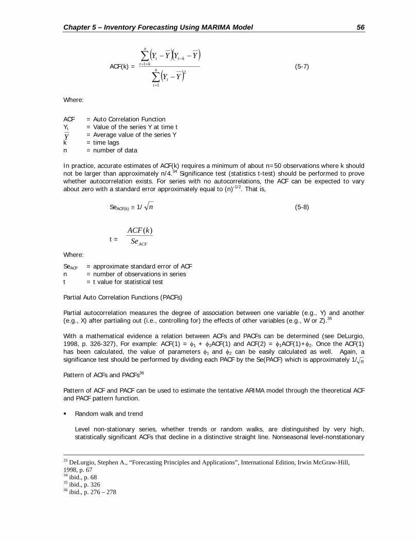
Chapter 5 – Inventory Forecasting Using MARIMA Model 56
ACF(k) =
( )( )
( )∑
∑
=
+=−
−
−−
n
tt
n
ktktt
YY
YYYY
1
2
1 (5-7)
Where:
ACF = Auto Correlation Function Yt = Value of the series Y at time t = Average value of the series Y k = time lags n = number of data
In practice, accurate estimates of ACF(k) requires a minimum of about n=50 observations where k should not be larger than approximately n/4.34 Significance test (statistics t-test) should be performed to prove whether autocorrelation exists. For series with no autocorrelations, the ACF can be expected to vary about zero with a standard error approximately equal to (n)-1/2. That is,
SeACF(k) ≅ 1/ n (5-8)
t =
Where:
SeACF = approximate standard error of ACF n = number of observations in series t = t value for statistical test
Partial Auto Correlation Functions (PACFs)
Partial autocorrelation measures the degree of association between one variable (e.g., Y) and another (e.g., X) after partialing out (i.e., controlling for) the effects of other variables (e.g., W or Z).35
With a mathematical evidence a relation between ACFs and PACFs can be determined (see DeLurgio, 1998, p. 326-327), For example: ACF(1) = φ1 + φ2ACF(1) and ACF(2) = φ1ACF(1)+φ2. Once the ACF(1) has been calculated, the value of parameters φ1 and φ2 can be easily calculated as well. Again, a significance test should be performed by dividing each PACF by the Se(PACF) which is approximately 1/
Pattern of ACFs and PACFs36
Pattern of ACF and PACF can be used to estimate the tentative ARIMA model through the theoretical ACF and PACF pattern function.
Random walk and trend
Level non-stationary series, whether trends or random walks, are distinguished by very high, statistically significant ACFs that decline in a distinctive straight line. Nonseasonal level-nonstationary
33 DeLurgio, Stephen A., “Forecasting Principles and Applications”, International Edition, Irwin McGraw-Hill, 1998, p. 67 34 ibid., p. 68 35 ibid., p. 326 36 ibid., p. 276 – 278
Y
ACFSekACF )(
n

Chapter 5 – Inventory Forecasting Using MARIMA Model 57
series have only one statistically significant PACF, at lag 1. The PACF(1) and ACF(1) values are equal and are typically very high.
Autoregressive (p,0,0)
The ACFs and PACFs of autoregressive process can be just as distinct as those of level non-stationary processes. However, the ACFs decline at an exponential rate, rather than in a straight line. PACFs are very important in identifying p and q in stationary series. An ARIMA (p,0,0) process has significant PACF spikes through p—lags.
Moving Average (0,0,q)
The ACFs and PACFs of ARIMA moving average models are also distinctive. The ACFs spike(s) can determine the order(s) of moving average model, while PACFs in moving average model behaves exponentially decline.
White Noise (0,0,0)
For white noise, no statistically significant ACFs and PACFs exist.
Prewhitening the Input Series
Prewhitening the input series consists of finding the ARIMA model for Xt that yields white noise residuals. By eliminating the auto-correlation in Xt, it is possible to better measure the correlation between of Xt and Yt. Supposed that white noise residuals are achieved from the following model:
xt = φ1xt-1 + et (5-9)
where xt is the deviation of actual value of the series at time t and the mean of series (Xt -µ ) while ets are white noise residuals. Re-expressing this relationship in terms of et yields:
et = xt - φ1xt-1 (5-10)
to avoid confusion with the residuals of other models and to facilitate further analysis, designate et as αt , therefore:
αt = xt - φ1xt-1 (5-11)
the series αt is referred to as the prewhitened input series xt because it is a white noise series.
Pretreating the Output Series
By treating yt exactly as xt was prewhitened, all of the direct cross correlation that existed before prewhitening is retained. That is, yt is transformed to a new series using the exact model of equation (5-11), which is:
βt = yt - φ1yt-1 (5-12)
the series βt is referred to as the pretreated output series yt because it has been treated identically to the prewhitened model of xt.
Backshift Operator
An efficient notation used for (M)ARIMA modeling, including differences, is the backshift operator B. By definition,
BkYt = Yt-k (5-13)

Chapter 5 – Inventory Forecasting Using MARIMA Model 58
Where B transform Yt backward k time period to Yt-k. All algebraic laws of exponents and polynomial expansions are valid with the backshift operator.37
Transfer Function MARIMA Model
The general transfer function equation is:38
yt = (5-14)
where yt and xt are called the output and input variables, respectively, ω0, ω1,…, ωs and δ1,…, δr are transfer function coefficients, B is the backshift operator of input variable (x) and Nt is a noise model. ω0 is the influence of input variables (xt) on the output variable (yt) in period t, while δ1 is the lagged influence of input variables (xt) on output variable (yt) through yt+k for k(number of lag)>0.
The form of transfer function is determined by three components, r, s and b. ‘b’ presents the dead time in which the numbers of impulse response equal to zero. ‘s’ is the order of the numerator ω(B) which captures unpatterned spikes in the impulse response graph plus decay start up value. While, ‘r’ is the order of the denominator δ(B) which presents the decay pattern of the impulse response. Impulse response is the weight of transfer function. This can be estimated through cross correlation function (CCF) pattern which will be discussed later.
Zero – Order Transfer Functions:
yt = (ω0 - ω1B)xt + Nt (5-15)
First – Order Transfer Functions:
(5-16)
Second – Order Transfer Functions:
(5-17)
Cross-Correlation Function (CCF)
The cross-correlation coefficient measures the strength of the relationship between output variable (Yt) and input variable (Xt-k), where k is a positive or negative integer representing the lag or lead relationship between these variables.39 When there are lag relationships between Xt-k and Yt, lagged values Xt-k provide an effective way to estimate the future values of Yt. The cross-correlation function (CCF) equals:
CCFxy(k) = (5-18)
Where: COVxy(k) = ; k ≥ 0 or (5-19)
37 DeLurgio, Stephen A., “Forecasting Principles and Applications”, International Edition, Irwin McGraw-Hill, 1998, p. 298 38 ibid., p. 535 39 ibid., p. 132
yx
xy
SSkCOV )(
∑+=
− −−n
ktktt XXYY
n 1))((1
trr
tsb
sbb
NBBB
xBBB+
−−−−−+− ++
)...1()...(
221
110
δδδωωω
ttt NxB
y +−
=)1( 1
0
δω
ttt NxBB
y +−−
=)1( 2
21
0
δδω

Chapter 5 – Inventory Forecasting Using MARIMA Model 59
COVxy(k) = ; k ≥ 0 (5-20)
COV stands for covariance. It is the mean of the product of the deviations of two numbers from their respective means. While, Sx and Sy are standard deviations of variable X and Y respectively.
Likewise the calculation of ACF, to measure the strength of the relationship between variables, it is recommended to use about 50 matched pairs data. And also like autocorrelations, stationarity is achieved when cross correlations decrease quickly.
CCFs are an important transfer function identification and diagnostic tool. The list of transfer functions given r, s and b can be seen in Appendix D.
Goodness of Fit ( )
After the MARIMA model is developed according to the development steps, the preliminary model should be diagnosed to confirm the effectiveness of the model. This will be done by calculating the Goodness of Fit ( ).
The is a measure of how useful the inputs (the X’s) are in explaining the movements of the output (Y).40 is calculated using the following equation:
= 1 - (5-21)
where:
Syx (or RSE) = (5-22)
Syx = the standard deviation of Y given X values Yi = actual value = fitted value of Y n = number of observation k = number of estimated parameters
However, in this case, to judge the relative advantage of the MARIMA model, will be calculated as follows.
= 1 - (5-23) where the underlying calculation of RSE is presented previously.
Once the model is convinced to be valid, then it is ready to be used to forecast.
For the detailed explanations of building both ARIMA and MARIMA model, please refer to the book of Forecasting Principles and Applications (De Lurgio, 1998).
5.4. Application of the Method to Unilever Case
Data
As explained in the beginning of this chapter, the purpose of developing a MARIMA model is to understand the accurate relationship between the inventory level as the dependent or output variable and the production quantity, the delivery and the sales order as the independent or inputs variables. By
40 Pankratz, Alan, “Forecasting with Dynamic Regression Models”, John Wiley & Sons Inc., 1991, p. 89
2R
2R
2R 2
2
y
yx
SS
knYYi
−
−∑ 2)()
Y)
2R
2R
2R
)()(
2
2
ARIMARSEMARIMARSE
∑−=
+ −−n
kttkt XXYY
n 1))((1
2R

Chapter 5 – Inventory Forecasting Using MARIMA Model 60
knowing the relationship accurately, it is expected that the company would be able to control its inventory level to achieve the daily inventory target.
To apply this forecasting method, the presence of historical data is essential. Those historical data will be used to calculate the parameters according to the MARIMA method. The data should satisfy both the quantity and quality requirements as has been discussed in performing sales order forecast in Chapter 4. Note that the ideal quantity of the data is minimal 50 data points for each variable for the purpose of calculates the degree of correlation in MARIMA model.
Looking back to the general requirement for the number of observation required for the inventory forecasting application, the method should be able to deal with the relatively limited data available since the product has just been launched. Comparing the requirement of performing the model and the data availability, a risk might arise that the MARIMA method was not suitable to be performed due to data unavailability. However, this new type of product has been launched for some months while the data period used for performing this inventory forecasting using MARIMA method is daily data. Since the model requires minimum 50 data points which is equal to 50 working days or 2 months approximately for 6 working days per week, the data should have been available. Consequently, the method is applicable in the company.
According to the generic MARIMA model (5-1), the list of data needed is as follows.
Table 5-1 List of Data for Performing MARIMA Model
Variable Name Dimension Description Stock Availability Level
Quantity/day This is the historical data of the inventory level in the product family aggregate level. This will be the dependent variable in this specific case.
Production Quantity Quantity/day This represents historical data of the production quantity in the product family aggregate level. This is one of the independent variables in this specific case.
Delivery Quantity Quantity/day This represents the historical data of the delivery quantity from manufacture to customers per day. This is also an independent variable and calculated by product family.
Sales order Quantity/day This is the historical sales order data per product family. This is one of the independent variables in this specific case.
In this study, due to the unavailability of the data needed, the calculation of stock availability forecasting using MARIMA model cannot be performed. The unavailable data occurs due to the company’s confidentiality policy and the difficulty in the environment of the cross-functions business interrelationship within the company’s network. This will be discussed further in the end of the report.
Steps to Forecast the Stock Availability Using MARIMA Model
Although the data is not available, here will be presented the steps needed to develop a forecast model using MARIMA model. However, since the MARIMA model has no generic model and the aim of the modeling process is to produce the specific model for a specific case, the following steps might be unclear without practicing in the real data. Therefore, an example of the calculation from the literature will be presented to help understanding the method and interpreting the model.
It should be noted that the aim of the following processes is to develop a MARIMA model for forecast the stock availability that follows the function presented in (5-1), while, the examples of the applications are only to help understanding the process.
Firstly, an ARIMA model for the output (Yt) should be developed prior to develop a MARIMA model. This ARIMA model of the output becomes a benchmark for judging the fit of the multiple input MARIMA model as well as a potential noise model. In the company’s case, the output is the quantity of the daily stock availability of the product in the product family aggregate level (e.g. sandwich, salad). To build the

Chapter 5 – Inventory Forecasting Using MARIMA Model 61
ARIMA model for those variables, there are 4 iterative steps that should be followed, which are (1) model identification, (2) coefficient estimation, (3) model and residual diagnostics and (4) forecasting verification and reasonableness.
Before using the data for forecast, it should be checked whether the data approximately normal distributed. This can be done through plotting the data series, using a scatter diagram and a histogram as well as the summary statistics. If the data series were not normally distributed, transformation should be considered, such as logarithms. The series should be cleaned from outliers as well. When outliers exist, the series should be adjusted before using it for developing a (M)ARIMA model. This has been discussed in the previous chapter.
In model identification, the series should achieve stationarity both for the level and variance, unless it will cause the (M)ARIMA identification problem because the strong autocorrelations that exists in the two series make it difficult to measure the cross corerelations between the series. Level stationarity is achieved when the mean of the series is the same over time; thus no differencing is necessary. While, a process that has a stationary variance has a constant variance over all observations. Variance is the expected value of the squared deviations. A transformation such as differencing and logarithmic or power transformation might be necessary to achieve stationarity in the series. When the series have achieved stationarity, the pattern of the series can be identified through graphs, statistics, ACFs and PACFs.
In coefficient estimation, the coefficients of the model are determined through software applications of least square and maximum likelihood methods. If the estimation procedure converges on good coefficients, the further procedures can be performed which is model and residual diagnostics.
In model and residual diagnostics, it should be checked whether the model results in a high value of to measure model accuracy and low value of BIC (Schwarz Bayesian Information Criterion) to determine the best from competing models. In addition to that, the Durbin Watson (DW) statistic which detects patterns in a series of errors should approximately give result of 2. Q-statistics should also be checked whether the group of autocorrelations is statistically different than those expected from white noise (Q-test > Chi-square table). With the support of software applications, those statistics measurements will be automatically provided. When the diagnostics confirm that the model is valid, then forecasts can be made by using this verified model. Otherwise, another alternative models should be developed. Last, the forecasts should be checked for the reasonableness.
A brief example of building an ARIMA model will be presented in the next box. The case is adopted from DeLurgio (1998) as an attempt to understand an ARIMA model.
Case Example 1: (Adopted from DeLurgio, 1998, p. 340-343) A firm seeks an ARIMA model for forecast the demand of its animal pharmaceutical. The monthly demand data over the last 13 years (156 data points) is plotted through a graph. The ACF(s) and PACF(s) are calculated through equation (5-7) and are also plotted. All of the calculations and graphs are illustrated in Appendix G. 1. Identification
From the plotted data and the calculations of ACF(s) and PACF(s) in Appendix G, it can be seen that this series has seasonality. This is shown from the ACFs which are dominant at lags 12, 24 and 36. In other words, it is recurrent every 12 period. The linear decline in seasonal ACFs indicates of seasonality non-stationarity. The large spike of PACF at 12 confirms of the need for twelfth-order seasonal differences to attain stationarity.
2. Estimation Comparing the calculations and plotted ACFs and PACFs in Appendix G with the theoretical ACFs and PACFs patterns in Appendix C, it leads to firstly estimate a twelfth-order seasonal autoregressive model. The tentative model is ARIMA(1,0,0)12: yt = φ12yt-12 + et (ex1-1) yt = 1.000yt-12 + et (ex1-2) The estimated coefficient (1.000) confirms that the level of this time series is seasonally non-stationary. This leads to estimate another tentative model with adding a trend (constant) coefficient. The underlying assumption of adding a trend coefficient is presented also in Table G2 Appendix G. The tentative model becomes: (1-B12)Yt = θ0 + et (ex1-3)
2R

Chapter 5 – Inventory Forecasting Using MARIMA Model 62
From the above example, an ARIMA model for stock availability could be developed through the four iterative processes as explained in the example. Likewise the forecast model in the example, there is also a probability that the forecast model for stock availability will involve seasonality factor due to the way the company handle the supply operation as explained in Chapter 4 and also trend factor. However, let an actual data set of stock availability quantity determines the inventory forecasting model through the ARIMA model building processes.
To develop a complete MARIMA model for the company case, there are steps should be followed. Firstly, the MARIMA models of output (Yt) and each input (Xi,t) should be developed. Therefore, in this case, there will be three models, which are (1) the MARIMA model for daily stock availability (Yt) and the daily production quantity (X1,t), (2) the MARIMA model for daily stock availability (Yt) and the daily delivery quantity (X2,t) and (3) the MARIMA model for daily stock availability (Yt) and the daily sales order (X3,t). These one-input MARIMA-models become a guide to structure the three-input MARIMA model of the stock availability (Yt) and the daily production, delivery and sales order (Xi,t).
In developing a MARIMA model, there are iterative steps of MARIMA model development, which include (1) identification, (2) estimation of the model, (3) diagnostics and (4) forecasting. The development of ARIMA model for the output that has been performed previously is one of the iterative processes in identification of the development of MARIMA model.
In identification process of the development of MARIMA model, after developing an ARIMA model for the output (Yt), ARIMA models for each input variable should also be developed with the same procedures that have been explained previously. The input variables will be the daily production quantity (X1,t), the daily delivery quantity (X2,t) and the sales order quantity (X3,t). These ARIMA models are developed in order to prewhiten the input variables and to pretreat the output variable (stock availability). Prewhitening and pretreating terms and procedures have been explained previously in equations 5-9 to 5-12. Prewhitening the input series is an attempt of finding the ARIMA model for Xt(input) that yields white noise residuals. While, pretreating is exactly the same with prewhitening, only it is done for the output (Yt). This will be used to develop a one-input MARIMA model.
3. Diagnosis
Table G3 in Appendix G presents the diagnostic statistics of the tentative model (ex1-3). The diagnostic statistics of this
model are favorable. The goodness of fit (2
R ) is high (0.963). It means that the model has explained or eliminated 96.3% of Y’s original variance. The RSE (Residual Standard Errors) is low (3.991), the DW statistics is approximately to 2 (2.143) and Q-statistics (25.407) is greater than the Chi-square statistics. They denote that the residuals are white noise. The constant coefficient,θ0, (2.0874) is very significantly different than zero, which is determined by the t-statistics. Thus, the annual trend exists. Residuals of this model should also be diagnosed. From the calculation and plotted of the residuals, the ACFs and PACFs of the residuals which are illustrated in Figure G4-G6 in Appendix G respectively, it could be concluded that there are no patterns or statistically significant coefficients in this table, thus white noise residuals are confirmed.
4. Forecasting After performing all those steps of building an ARIMA model, the model of demand forecast of animal pharmaceutical is ready. The model is as the following: 012
ˆ θ+= −tt YY (ex1-4)
To forecast m period ahead, the model is:
087.2ˆˆ12 += −++ mtmt YY (ex1-5)
Interpretation: The forecasting model (ex1-5) expresses that the forecast value of series Y for m period ahead is determined by the value of series Y twelfth periods behind the projected time (t+m-12) due to twelfth-order seasonality, plus the annual trend of 2.087.

Chapter 5 – Inventory Forecasting Using MARIMA Model 63
Next, the CCFs (Correlation Coefficient Function) of pretreat series (βt) and prewhitened series (αt-k) should be performed to identify the ‘r’ (the order of denominator in the transfer function), ‘s’ (the order of numerator in the transfer function) and ‘b’ (the dead time of the impulse response). ‘r’ is identified just as with univariate ACF patterns for AR(p) models. ‘b’ is identified at the first significant CCF(k) is encountered. While, ‘s’ is determined in which from ‘b’ to ‘b+s’ the CCF(k) are significant but no specific pattern may exist.
After identification of ‘r’, ‘s’ and ‘b’, the next procedure of the estimation of a model could be examined. Given the ‘r’, ‘s’ and ‘b’, the estimation of the transfer function can be identified. The examples of transfer functions with given ‘r’, ‘s’ and ‘b’ are presented in Appendix D. The residual of the estimated transfer function then is used to identify the noise model.
The next procedure is to diagnose the tentative model of the one-input MARIMA model. Likewise in ARIMA modeling, diagnostic statistics are used to confirm whether the model is valid, otherwise the model should be modified. Some diagnostics that should be performed are the confirmation of the significance level of parameters incorporated in the model, the confirmation of the white noise residuals, the confirmation that the residuals are not crosscorrelated with prewhitened series (αt-k) and the fit of the model by overfitting the other models. If the tentative model presents that it is valid and reasonable, then it can be used to develop the three-input MARIMA model.
The three-input-MARIMA model is structured using the one-input MARIMA models. When the tentative three-input MARIMA model is ready, this model should be diagnosed through diagnostic statistics likewise in one-input MARIMA model. Then, the effectiveness of the model should be confirmed through the
goodness of fit calculation (2
R ). To judge the relative advantage of the MARIMA model, a calculation of 2
R for the MARIMA versus the ARIMA model for output can be performed.
A brief example of building a MARIMA model will be presented in the next box. The case is adopted from DeLurgio (1998) as an attempt to understand a MARIMA model.
Case Example 2: (Adopted from DeLurgio, 1998, p. 562 – 571) An automobile firm seeks a MARIMA model to forecast its market share with the relationships with advertised quality and price ratio. The variables and the descriptive statistics for the output and inputs are as follows while the complete graphs and calculation are presented in Appendix H. Yt = f(X1t-k, X2t-k, Yt-k, et-k) (ex2-1) Where: Yt = market share of the manufacturer (%) X1t = ratio of the amount spent on advertising its quality improvements to industry advertising expenditures (%) X2t = ratio of the firm’s prices to the average of industry prices (%)
Series Observation Mean Std. Deviation Minimum Maximum Yt = MARKET (%) 100 22.817 4.886 15.034 31.692 X1t = ADVERT (%) 100 0.18888 0.05169 0.09510 0.31280 X2t = PRICE (%) 100 1.19711 0.17552 0.89554 1.48422
The Plot of the series are presented in Figure H1, Appendix H. 1. Univariate (ARIMA) Model of the Output Yt.
The output of the series appears to be very random (Figure H1 in Appendix H). By using the procedures of developing an ARIMA model as has been explained in the case example1, the ARIMA model of the output (Yt) is determined as a random walk model, ARIMA (0,1,0):
Yt = Yt-1 + et (ex2-2)
With: n =100; SYt = 4.91; RSE = 0.9296; 2
R = 0.964; DW = 2.149; Q = 25.407; Significant of Q = 0.3839
Since the DW is approximately 2 (2.149) and the level of Significant of Q (0.3839) > 0.05, thus the residuals are white
noise with a high 2
R of 0.964 which means that the model has explained/eliminated 96.4% of the output variance.

Chapter 5 – Inventory Forecasting Using MARIMA Model 64
The 2
R will be compared with the one- and two-input MARIMA model developed next.
2. ARIMA model for the prewhitened of advertised quality (X1t)
Also using the same procedures of developing an ARIMA model, the univariate analysis of the advertising ratio yields the following model:
(1 - φ1B)(1 – B) X1t = α1t (ex2-3)
(1 – 0.3885B)(1-B)X1t = α1t (ex2-4)
(t-stat = - 4.17)
with: n = 100; SX1t = 0.0522; RSE = 0.00853;2
R = 0.973; DW = 1.95; Q = 24.48; Sig. Of Q = 0.3778; α1t = residuals et
This model is appropriate since the RSE is low (0.00853), the DW is approximately 2 and level of Sig.of Q is > 0.05, thus it confirms that the residuals are white noise. The parameter coefficient (φ1) is significantly different than zero, moreover, it
has high value of 2
R (0.973).
3. MARIMA model for Yt and X1t (between the prewhitened X1t and pretreat Yt).
The MARIMA model should be identified from the prewhitened X1t and pretreat Yt. Therefore, the output variable (Yt) should be pretreat prior to develop the MARIMA model accordingly to the prewhitened X1t that has been developed previously (ex2-4). The pretreat of Yt results in the following calculation.
(1 – 0.3885B)(1 – B)Yt = β1t (ex2-5)
To identify the MARIMA model, the CCF (Cross Correlation Function) of the prewhitened α1t and the pretreat β1t is calculated. The results are presented in Table H1 in Appendix H. It shows that the significant CCF is at lag 1, thus β1t and α1t-1 is correlated. Having compared this pattern with the theoretical CCF pattern which is presented in Appendix D, the suggestion model is MARIMA (0,0,1) with: r = 0, s = 0 and b=1.
)1(
1 10 Be
XY ttt −
+= −ω (ex2-6)
)1(
172.20 1 Be
X tt −
+= − (ex2-7)
(t-stat=2.117)
with: n = 99; SYt = 4.91; RSE = 0.896; 2
R = 0.967; DW = 2.21; Q = 20.54; Sig. Of Q = 0.6656
This model is appropriate since the residuals are white noise as measured by the DW and Q statistics, and the t-value of the parameter shows that the coefficient is significantly different from zero (t-stat significance = 0.36). While not shown, the ACFs and PACFs of the residuals of this model have no pattern, thus the noise model is appropriate for an ARIMA (0,0,0). CCFs between et of equation (ex2-7) and α1t of equation (ex2-4) are also calculated. The result is presented in Table H2. It shows that there is no cross correlation between those two residuals, thus this model is best for relating output and advertising ratio.
4. ARIMA model for the prewhitened of price ratio (X2t).
Using the same procedures of developing an ARIMA model, the univariate analysis of the prewhitened price ratio yields the following model:
(1 - φ1B)(1 – B) X2t = α2t (ex2-8)
(1 – 0.46615B)(1 – B)X2t = α2t (ex2-9)
(t-stat = - 5.308)
with: n = 100; SX2t = 0.1757; RSE = 0.0221; 2
R = 0.984; DW = 2.04; Q = 26.22; Sig. Of Q = 0.2904; α2t = residuals et
The DW and Q statistics show that the model is white residuals, the t-statistic is greater than the t-value, thus the coefficient is significantly different than zero. This model is an appropriate ARIMA model for the prewhitened price ratio.
5. MARIMA model for Yt and X2t (between the prewhitened X1t and pretreat Yt)
Prewhitened α2t has been calculated previously. Pretreat output β2t is calculated as follows.
(1 – 0.46615B)(1 – B)Yt = β2t (ex2-10)

Chapter 5 – Inventory Forecasting Using MARIMA Model 65
To identify the MARIMA model, the CCF (Cross Correlation Function) of the prewhitened α2t and the pretreat β2t is calculated. The results are presented in Table H3 in Appendix H. It shows that the significant CCF is at lag 1, thus β2t and α2t-1 is correlated. The suggestion model is MARIMA (0,0,1) with: r = 0, s = 0 and b=1 as follows.
)1(2 10 B
eXY t
tt −+= −ω (ex2-11)
)1(
209.16 1 BeX t
t −+−= −
(ex2-12)
(t-stat= - 4.942)
with: n = 100; SYt = 4.91; RSE = 0.8195; 2
R = 0.9722; DW = 2.76; Q = 43.50; Sig. Of Q = 0.087
The model has a high 2
R (0.9722) and significant t-statistics. However, the DW is not approximately 2, and level significance of Q show that the residuals are not white noise. The calculation of ACFs and PACFs of the residuals which is presented in Table H4 shows that the residuals have an MA(1) pattern, thus this pattern should be added in the equation (ex2-12). Because the CCFs of et and α2t in Table H5 do not show any patterns, the model is refitted with an MA(1) model. The estimation of the model is MARIMA (0,0,1) as follows.
)1(
)1(2 110 Be
BXY ttt −
−+= − θω (ex2-13)
)1(
)6536.01(222.22 1 BeBX t
t −−+−= −
(ex2-14)
(t-stat = - 14.6) (t-stat= - 8.367)
with: n = 100; SYt = 4.91; RSE = 0.7069; 2
R = 0.9793; DW = 1.95; Q = 16.60; Sig. Of Q = 0.828
The 2
R is higher than in univariate analysis (equation ex2-2), but from CCF calculation in Table H6, there is a near significant at lag 1 that might denote a deficiency in the transfer function. Looking back to the CCF of β2 and α2t-k in table H4, the CCF(1) and CCF(2) identify an exponential decline, therefore a first-order transfer function should be tried. The tentative model is as follows.
)1(
)1()1(
21
1
10
Be
BB
XY tt
t −−+
−= − θ
δω (ex2-15)
)1()7515.01(
)4705.01(246.13 1
Be
BX tt
−−+
−−
= − (ex2-16)
with: n = 100; SYt = 4.91; RSE = 0.6539; 2
R = 0.9823; DW = 1.94; Q = 20.78; Sig. Of Q = 0.594
The BIC (Bayesian Information Criterion) is used to assist the decision which one is the model better model, whether equation ex2-13 or ex2-15. For the calculation of BIC is presented in Table H7 in Appendix H. The BIC calculation shows that equation ex2-15 is the preferred model because the BIC value is smaller.
6. MARIMA model of Yt = f(X1,X2)
From the one-input MARIMA models that have been developed, the two-inputs MARIMA model is developed which results in a tentative model as follows.
)1()1(
211
1'0
10 BN
BXXY tt
tt −+
−+= −
− δωω (ex2-17)
The diagnosis statistics are presented in Table H8 in Appendix H. This table shows that all coefficients are statistically significant but the residuals are not white noise. With the calculation of ACFs which is presented in Table H10, it is showed that this model has an MA(1) pattern. Thus, an MA(1) model is added to equation (ex2-17) to yield equation (ex2-18).
)1(
)1()1(
21 11
1'0
10 BeB
BXXY tt
tt −−+
−+= −
− θδ
ωω (ex-2-18)
7. Diagnostics of the MARIMA model
Table H12 in Appendix H shows that the model is a good one since all diagnostics statistics of this model satisfies the criteria. Also, table H13 and H14 present that there are no patterns left between the prewhitened input variables and these residuals. The effectiveness of the model is calculated following the equation 5-23. This is a fraction between the RSE of the univariate of Yt which has been calculated in equation ex2-2 and the full MARIMA model in equation ex2-18. The result is as follow.
%09.656509.09269.05476.01 2
22==−=R (ex2-19)

Chapter 5 – Inventory Forecasting Using MARIMA Model 66
Interpretation of the Model After completing the development of the MARIMA model for the case example, the end result should be interpreted to give an understanding of the underlying processes involved in the value of the series (the market share value). For this purpose, Equation (ex2-18) should be re-written without backshift operator. It is done by multiplying the both sides with (1-δ1B)(1-B) to yield the following equation: Yt = Yt-1+.377(Yt-1-Yt-2)+.1691(X1t-1-X1t-2)+.06375(X1t-3-X1t-2)+.1496(X2t-2-X2t-1) +et – .3770 et-1 + .9409(.3770 et-2 – et-1) (5-24) The above equation explains the affecting factors and the degree of affection of those factors to the market share (Yt). The market share (Yt) is determined by its previous values, the amount spent on advertising (X1t) and the price factors (X2t) in the following manner. The market share (Yt) equals an autoregressive of its previous actual value (Yt-1) plus the differences between its actual value at time (t-1) and (t-2) with a fraction (.377). This difference could be interpreted as the trend that involved in the market share series. The market share (Yt) is also determined by the amount spent on advertising (X1t). It is added with the differences between the amount spent on advertising at time (t-1) and (t-2) plus the difference between the amount spent on advertising at time (t-3) and at time (t-2) with some fractions, which are .1691 and .06375 respectively. While, the differences between actual price (X2t) at time (t-1) and (t-2) also determine the market share (Yt) with a fraction of .1496. The errors between the forecast value and actual value at time (t-1) and (t-2) also contribute to the value of market share at time t (Yt). It seems that the affect of the amount spent on advertising (X1) to the market share (Y) at time (t-2) always gives a negative fraction compared to the amount spent on advertising at time (t-1) and (t-3). This indicates that an oscillation exists in the series of the amount spent on advertising (X1). The affect of the advertising at period t (X1t) will increase the market share with one lagged period (Yt+1). However, due to the sales increase in that period (t+1), it will decrease the sales in the next two periods (t+2). Perhaps, it happened since people bought the product at time (t+1), so that they had enough stock at time (t+2). But, the sales is increasing again in time (t+3) as the people started buying the product after their stock was decreasing. The affect of the price (X2t) to the market share (Yt) is quite apparent that when the price was set to be cheaper than the previous price (X2t-1 < X2t-2), it will increase the market share by the fraction of .1496.
The errors term (et, et-1 and et-2) is used to modify the forecast based on the weighted averages of the one- and two- step ahead forecast errors (disturbance values) that would occur if only the advertising (X1t) and the price factor (X2t) were used to forecast the market share (Yt).
The closest lag in the relationship between the market share (Yt) and the amount of advertising (X1t) and the price (X2t) is one-period lag. Therefore, one-period-ahead forecasts should have nearly the accuracy of the fit.
5.5. Final Remarks
Since the forecasting calculation of the stock availability cannot be performed, this chapter is aimed to give an introduction to modeling and forecasting stock availability using MARIMA model. The given examples help to understand forecasting using the (M)ARIMA model. As can be seen from the example, this model has greatest advantages of modeling the lagged involved between the independent variables and dependent variable.
The calculation of 2
R means that a 65.09% increase in the explained variance from the MARIMA model over the ARIMA model. This increase is quite high. Thus, it can be concluded that the MARIMA model in equation ex2-18 provides good method for forecasting market share.

Chapter 5 – Inventory Forecasting Using MARIMA Model 67
To forecast the dependent variable using the MARIMA model, the future value of each independent variable should also be predicted beforehand. This could be done by performing the univariate ARIMA models for each independent variable which have been developed accompanied the MARIMA model building. An instance taken from the given example case tells that to forecast the market share (Yt) using Equation (ex2-18), the future value of the amount spent on advertising (X1t) and the price (X2t) should be determined in advance. They could be predicted using Equation (ex2-4) and (ex2-9) respectively. Nonetheless, the independent variables could also be a control variable. In this case, the value of this independent variable is determined by the company, therefore, performing ARIMA for this variable might be unnecessary. For example, the price could be determined directly when it is known to be increase or decrease in the certain projected time (X2t). In this case, the price was not necessarily determined through the ARIMA model performance.
The given example model could be used for a control tool in the following manner. Supposed that the company had a certain target of the market share to be achieved in the certain targeted time (Yt). Meanwhile, the company had control on the amount of money spent on advertising (X1t) and on the price of the product (X2t). Using the model in Equation 5-24, the company would be able to predict the future value of the market share through the given values of the amount spent on advertising and the price. Then, the company could compare this projected value with the target whether the target would have been achieved as desired in the projected time. Otherwise, the company could take necessary actions or develop scenarios, for instances adding more money for advertising, lowering the price or a combination of both policies such as adding more money while increasing the price, etc. This is done until the desired target would likely to be achieved. This enables the model to be a potential forecasting and controlling tool.
Supposed that the given example of MARIMA model was applied to the case of forecast and control short life span products, the variables involved in the MARIMA model would be as follows. The dependent variable (Yt) was the stock availability, while the independent variables were the production quantity (X1t), the delivery quantity (X2t) and the sales order quantity (X3t). The production quantity might contribute to the accumulation of the stock availability, while the delivery quantity would reduce the stock availability. A trend would be expected to consist in the sales order series. However, the contribution of the sales order to the inventory could not be predicted without using a real data set. Meanwhile, the implication of this method to the stock availability control system will be explained as follows. The company should determine a daily target inventory level (stock availability). The stock condition is forecast through the predicted future value of the sales order (X3t) and the determination of the future values of the production quantity (X1t) and delivery quantity (X2t). The univariate ARIMA model could be used to forecast the sales order (X3t). While, the company could determinate the value of the production quantity (X1t) and delivery quantity (X2t) since those are the control variables. The result of the predicted stock condition will be compared with the daily target inventory. The company would be able to determine the production and delivery quantity until the stock condition achieving the desired level.
The production, delivery and sales order quantity factors were expected to affect the stock availability with some time lags. The closest lag(s) consist in the model would determine the forecast period in which expected to yield the nearly most accurate of the fit. The given case example presented that one-period-ahead forecast should have nearly the accuracy of the fit since the closest impulse responses of the amount spent on advertising (X1t) and the price (X2t) consist of one-period lag.
Having considered the iterative steps that should be performed in developing a forecasting model with MARIMA method (both iterative steps in ARIMA and MARIMA) and considering that every model is developed for one specific case, this method is suitable for the aggregate level instead of item level. Performing ARIMA or MARIMA model for item level is inefficient since it is very time consuming and it is inefficient to maintain and perform forecasting for each item using different model.
To summarize, it is quite clear that the stock availability is one of the most important factors that should be managed in handling the short life span products. The MARIMA model is perceived to be potential in forecasting and control the stock availability as its ability to model time lags that mostly involved in the control application. The time lag, especially the closest lag period, is also useful to identify in which

Chapter 5 – Inventory Forecasting Using MARIMA Model 68
period the forecast is expected to be nearly most accurate of the fit. In MARIMA model, the future value of the dependent variable is predicted using some control or independent variables. In this case, the dependent variable is the stock availability and the control or independent variables are production quantity, delivery quantity and sales order. Prior to forecast using the MARIMA model, the values of independent variables should be predicted. This could be done using the univariate ARIMA model in which developed along with the MARIMA model development. It could also be directly determined if it was a control variable which was under the company’s control to change. Having considered the complexity of the development of a MARIMA model which includes modeling the errors, this method is potentially able to yield an high accurate forecast. However, the iterative steps and complexity involved in developing this kind of model makes it only suitable to be applied for the aggregate product level such as product family rather than item level.
69
Chapter 6. Product Availability Forecasting Model Using System Dynamics
6.1. Introduction
It has been identified in Chapter 3 that the product availability in the market is also one of the important variables to be controlled to ensure that undesired stock condition can be avoided. For short life span products, it is sensible that the company desires to have a short distribution chain to keep the freshness of the product. As a consequence, the distribution channels can be divided into two groups, which are the distribution to the distribution centers of the chained retailers and the distribution to the independent retailers (shops) or perhaps direct to vending machines in the future. In this case, the shorter the distribution chain means that the company may have more direct control to the product available in the market.
Meanwhile, it also has been presented that product availability in the market is the result of a complex system where involves causal relationship of processes in the supply chain. Moreover, the availability of the product in the market is not only the result of the physical goods transfer. It is also involving company policies and decision on their supply chain management both operational decisions such as the decision of the production quantity and strategic decisions such as delivery priority to certain channels.
Modeling this forecast problem with pure mathematics methods will involve an intricate and large number of calculations besides the difficulty to incorporate non-quantitative information to the model. Consequently, forecasts will ineffectively support the decision maker in controlling the system of interest. In addition to that, the intention of controlling the product availability in the market is not to calculate the exact value of the product in the market since this not giving added value to the company. However, it is done to give more understanding of the behavior of the stock in the market to support the company in designing or improving the supply chain operation in order to ensure that the desired stock behavior is achieved. Fortunately, system dynamics approach can be developed to model the system thinking of a complex demand-supply system. It is able to present the predicted future behavior of the system and also the possibilities to influence the system behavior, thus it would effectively support the decision maker in controlling the system.
The development of the system dynamics model in this study is to introduce the system dynamics method to the company as one of the forecasting and control methods. It is very useful in the long term forecast to support the company in making decisions in designing the supply chain operation so that their objectives regarding stock availability are achieved. Due to the limitation of time and lack of data availability, the complete use of the system dynamic model in the company cannot be performed.
The presentation of the theory of system dynamics is mainly adopted from Daalen (2001) and Sterman (2000).
6.2. General Requirements
A system dynamics study is chiefly intended to gain understanding, describe and explain observed developments and providing an understanding of possible (future) behavioral forms and possibilities to influence this.
In developing a model using system dynamics modeling, there are some steps should be followed, which are:
1. Problem identification

Chapter 6 –Product Availability Forecasting Model Using System Dynamics 70
Problem identification is the first step in model development. The objective of the study should be determined to understand what the real problem is and how it should be analyzed and how the model could support the decision-making.
2. Model Conceptualization
The conceptualization phase results in one or several graphical conceptual model which is the basis for a quantitative analysis of the system as well as qualitative analysis of the system behavior. Here the model objective and function is determined. The steps that are performed during the conceptualization phase are (1) determine model boundaries and identifying the important variables, and (2) creating diagrams of the major mechanism, including feedback loops describing the behavior of the system.
3. Model Formulation (Specification)
The formulation phase results in a quantitative model. Formulation means that a conceptual model is transformed into a formal quantitative representation.
4. Verification and Validation
In order to check whether the model is an appropriate model which means the model describes the reality and can be used as a decision making tool, verification and validation should be performed. Verification is used to refer to consistency and the aim of perform verification is to ensure that no errors have been made in representing the model in the computer. Validation is used to refer to usability. The model should produce the right output behavior for the right reasons.
5. Model Use
When the model is completely ready, the model can be used as per the objective that have been specified previously. There are two ways in using the model as the decision making tool, firstly is by changing the parameters in the model and secondly is by changing the structure of the model. In here, the behavior of the model is studied to get an understanding of the effect due to the changes either in parameters and structure of the system.
6.3. General Structure of System Dynamics Model
Feedback
Basic principle of system dynamics that the behavior of system in principally caused by the structure of the system. The structure not only contains all physical aspects but also includes policies and information that are important in decision making process. Such a structure contains gains, delays and information feedback, where feedback concept is one of the essential characteristics of system dynamics.
Feedback means that a two-way causalties exists, one variable affects the other variable and vice versa. These influences can take place directly or indirectly through other variables. The consequences of the influences may become clear quickly or after some time, thus close loops and delays are characteristics for all feedback processes. A feedback system consists of two or more connected feedback loops. There are two types of feedback relations: positive and negative feedback. A positive feedback loops result in a continuous increase or decrease of the value of variables, while a negative feedback loops can show goal-oriented behavior.
System Dynamics Diagram
The system dynamics is presented using the system dynamic diagrams or ‘pipe’ diagrams to represent system. The concept of system dynamic flow diagram are levels and rates. Levels represents parts of the

Chapter 6 –Product Availability Forecasting Model Using System Dynamics 71
system in which accumulation occurs. Rates cause the value of a level to change. The dimension of a rate is usually expressed in units per time unit. The flow diagram shows that the rates causing the value of a level variable to decrease flow out of the level, so to peak, whereas in the causal diagram these variables are represented as a negative influence.
In representing the system diagram, there are numbers of software can be used, such as Vissim, Powersim, iThink and Dynamo. Each software has its own specific features. The figure below shows an example using Powersim convention. Basically, in the modeling there are four building blocks: level (representing the system state), flow (representing rate, filling or depleting the level), auxiliary (as converters) and the connectors (connecting the different blocks). Level is represented as a box, flow as a double arrow line with valve flow into (or out of) the level, auxiliary as a circle, and connectors as arrow line connecting different system components.
∫ += )0(.)( XdtdXtX
))(( tYfdX =
))(()( tXgtY =
Figure 6-1 Basic Building Block for System Diagram in Powersim
All the above variables can be time dependent functions or not time dependent. X(0) for example means the initial state of the level value. The stock level X(t) accumulates by integrating the flow rate (dX). Auxiliary variables (Y) control or convert other entities (g(X(t)).
The auxiliary can be presented in different forms, as a graphical function, or as a delay function. Different symbols will be used to indicate this representation. These converters are often computed and serve as intervening variables in the close loops that connect stock to flow. Connectors provide the linkage between different system components, reflecting the modeler’s assumptions about the causal relationship underlying the system. For more detail explanation about the representation of the diagram using Powersim, please refer to the Powersim manual.
6.4. Application of the Model to Unilever Case
6.4.1. Problem Identification
In dealing with a short life span type of product, inventory control is highly important to ensure that the products meet the requirement to avoid undesired stock conditions which are either over stock or stock out conditions. The inventory management is closely corresponding to the supply chain operations performed by the company. Meanwhile, a short life span type of product is a new experience for the company; thus, the supply chain operation for this type of product is still in the development. Considering that an effective design can be achieved when the company is able to predict the future events that affected by any decisions that taken with respect to the supply chain process, a system dynamics model is introduced to help the company in designing its supply chain operation. In this case, the objective of designing the supply chain operation is to achieve the desired conditions of inventory and product availability in the market in the aggregate product level.
X
dx
Y

Chapter 6 –Product Availability Forecasting Model Using System Dynamics 72
6.4.2. Model Conceptualization
In this chapter the causal diagram is constructed and the ideas behind each of the diagram is presented. The model is presented in 4 different sections which are production, distribution center inventory, inventory in vending and forecast demand. Though this separation does not mean to be a clear separation, rather to make an easier presentation and communication of the idea of the models. Most of the basic idea of the model is adopted from Sterman (2001) since he has developed a generic model for manufacturing or production environment in the aggregate level to demonstrate the supply chain dynamics. His model is general and applicable to a variety of manufacturing companies.
Conceptual Model for the Production
The production process is modeled and described in Figure 6-2 with the explanation as follows.
In the production process, the raw materials which determined as the production start rate are transformed to be finished products. During this process, materials flow through some processes, which described as WIP (Work In Process). This process incorporates a delay time in which the required time to manufacture a product.
The desired production start rate is determined by the desired production quantity and the WIP adjustment. The WIP adjustment or production backorder is derived from the discrepancy between the desired WIP and the desired production quantity, for instance discrepancy due to the production capacity constraint. An information delay is incorporated in determining the WIP adjustment. The WIP adjustment is incorporated as an attempt for the company to achieve the desired level of production. This creates a balancing (B) loop in the manufacturing process.
Figure 6-2 Causal Diagram For the Production
The desired production quantity is governed by the sales order forecast and the inventory adjustment between the desired inventory and the actual inventory level. Both factors influence the desired production quantity in the same direction. Likewise the WIP adjustment, the inventory adjustment is the result of a discrepancy between the desired inventory and the actual inventory level, which will be explained further in the inventory causal diagram as the second balancing loop in the manufacturing process for controlling the inventory. The sales order forecast is determined by the actual order with
From Demand Forecast
WIP Finished Product Rate Inventory Level
Inventory Adjustment
Desired Inventory
sales orderForecast
Desired ProductionQuantity
Desired WIPProduction Start Rate
Desired Production StartRate
Production Capacity + + +
delay
-+
++
+
+
WIP Adjustment
delay
-
+
+
+
+
B
inventorycontrol
B
WIP control

Chapter 6 –Product Availability Forecasting Model Using System Dynamics 73
some information delays. This will also be explained further in the causal diagram of the demand forecast.
As explained previously, the inventory level is governed by the production quantity rate. Thus, the production control plays an important role for the company to achieve the desired inventory level. The company could determine the desired level of production to ensure the adequacy of the desired inventory level. The control variable would be the production start rate, while the exogenous variable could be the availability of the raw material. However, the availability of the raw material is not meant to be the focus of the study, thus it is not modeled. The limitation of the raw material is assumed known in advance so that the company would be able to calculate the maximum production rate due to the inadequate raw material. The maximum production rate is summarized in the production capacity to limit the production start rate whenever it is necessary. Last, the company would be able to respond sufficiently quickly to deviations from the desired condition of the production (WIP) and the actual WIP through the WIP adjustment in order to achieve an in time adjustment.
Conceptual Model for the Distribution Center Inventory
Figure 6-3 presents the causal diagram of the underlying processes of inventory in the distribution center with the explanation as the following.
The inventory level within the distribution center is governed by the finished product rate from the production and the actual delivery to customers. The finished production rate is the acquisition rate while the actual delivery is the loss rate for the inventory level. The desired delivery to customer is determined by the forecast demand and will determine the delivery to customer as long as the inventory is available. Therefore, the actual delivery to customer is determined either by the maximum delivery rate (available inventories) or the desired delivery rate.
In order to control the inventory level to the desired level, the discrepancy between the desired inventory and the actual inventory level is incorporated in the model. This discrepancy will be reported as the inventory adjustment for a production request. This kind of report involves an information delay time. This creates a feedback loop of inventory control. The desired inventory level is governed by the desired inventory coverage to cover the sales order forecast for a certain projected period, plus the safety stock that will cover the forecast errors. In this case, the policy of safety stock will determine the desired inventory coverage.
Figure 6-3 Causal Diagram for the Distribution Center Inventory
From/To Production
From/To Demand Forecast
Production Finished Product Rate Inventory Level
Delivery to non vending
Delivery to vending
Sales Order Vending
Sales Order non vending
Total desired order
actualdelivery
servicelevel
Forecast Demand
maximum delivery rate
minimum orderprocessing time
safety stock
desired inventorycoverage
inventory adjustment
desired inventory
+ +
+
+
+
+
+
-
+
+
+
delay
++
+
+
+
delay
+
-
+ -
R
stockout
B
inventorycontrol

Chapter 6 –Product Availability Forecasting Model Using System Dynamics 74
The desired delivery is governed by the sales order from the customers. The sales order will be used to forecast the sales order in the future with an information time delay is incorporated within the process. This forecast will later be used to determine the desired production quantity.
In controlling the inventory within the distribution center, the objective is to keep the level of the inventory in a certain level that adequate to cover the average sales order and the safety stock due to unforeseen demand. This is represented in the desired inventory level variable. The adequacy of the inventory level should be determined by the company as one of its policies. In order to achieve the desired inventory level, the company could influence for instances the safety stock coverage or minimum order preparation time. The effects of a change in one or more of the control variables should also be known clearly to anticipate both the intended and unintended effects due to the policy imposed by the company, especially in the inventory level. Moreover, the external factors such as sales order forecast should also be known clearly in order to understand how it would affect the inventory level. Finally, the model is design to support the company to respond sufficiently quickly to deviations from the desired inventory level through the inventory adjustment variable in order to adjust in time.
Conceptual Model for the Vending Inventory Section
The causal diagram of the underlying processes of inventory in the vending machines is presented in Figure 6-4, while the explanation is as follows.
The actual inventory level in the vending machine is increase due to the delivery from the distribution center to the vending machine and decrease due to the sales to consumer. Since the sales rate to consumer is governed by the stock availability, a maximum sales rate in which depends on the stock availability in the vending machine is incorporated in the model. The more products sold to the consumer will reduce the inventory level. This creates a stock out feedback loop in the vending control.
The desired inventory in the vending machine is determined by the desired inventory coverage that covers the consumer sales within the replenishment cycle and safety stock due to the errors in consumer sales forecast.
Figure 6-4 Causal Diagram for the Customer Inventory
In order to control the inventory level in the vending machine, the discrepancy between the desired inventory and the actual inventory in the vending should be taken into account and reported as the inventory adjustment with an information time delay. This inventory adjustment will determine the
To Demand Forecast Delivery to vending inventory vending sales to consumer
desired sales to consumer
consumer sales rate
sales forecast to consumer
desired inventory coverage
replenishment cycle time
safety stockdesired inventory vending
adjustment inventoryvending
maxium sales rate
desired order vending
vending capacity
order vending
sales order
vending service level
++
-
+
+
delay
delay
-
+
+
+
++
+
+
+
delay
+
B
replenishment control
B
stock out vending
+
+sales order
process

Chapter 6 –Product Availability Forecasting Model Using System Dynamics 75
desired order from vending. This will cause a feedback loop to control the inventory through a replenishment activity. However, the desired order could be limited by the vending capacity, thus reduce the actual order from vending to manufacture. The sales order from vending is also determined by the consumer sales forecast.
The inventory in vending machine is given a special attention based on an assumption that the company has more direct responsibility for the inventory in a vending machine. The first step to control the inventory for the vending machines is similar to the inventory control within the distribution center, which is to determine the objective of the desired level of inventory in the vending machines. However, in directing the process into the desired level in the vending machine, the company is not able to influence how many products to be sold to the consumer since the consumer go directly to the vending machine and choose the product based on their preference without any control from the company. The only control variable for the company is to determine the delivery rate to the vending machines to make sure that the inventory is adequate to cover the consumer demand and some safety stock. The delivery rate could be influenced for instance through a policy decision of the replenishment cycle time or the order quantity from vending-customer. The consumer demand as the external factor should be known clearly to understand its affect on the vending inventory, for instance to calculate whether the current vending capacity is enough to serve the consumer demand. Finally, this model is also design to support the company in responding to any deviations from the desired and actual condition in a sufficiently quickly time through the vending inventory adjustment variable in order to avoid late adjustment performance.
Conceptual Model for the Sales Order Forecast
This causal diagram presented in Figure 6-5 is not aimed to present the sales order forecasting process, instead to represent the elements involved in the sales order forecasting.
The sales order forecast is determined by the historical of the total customer order rate. This total order is smoothed as an attempt to distinct the trend and seasonality elements since it is presumed that the demand of refrigerated prepared food products will involve seasonality and trend pattern as identified in Chapter 4. Then, this model will calculate the sales order forecast by involving the trends and seasonality factors. The sales order forecast is going to be used as the input for production and inventory control processes.
Figure 6-5 Causal Diagram for the Sales Order Forecast
To Production
order vending order non vending
total order
sales order forecast
trendseasonality
+ +
smoothed order
delay
+
+
-
+
-
++
+desired production
+

Chapter 6 –Product Availability Forecasting Model Using System Dynamics 76
6.4.3. Model Formulation
Data for the Simulation Model
The table below presents the data needed for the input of the simulation. The data should be obtained from an observation of the real condition and calculations.
Table 6-1 Input Data for the Model
Variable Dimension Description Production Production capacity Quantity/day This variable is the amount of maximum production rate
per day due to the limitation of machine’s capacity, labor and raw materials.
Manufacturing Cycle Time
Hours This is the time needed to produce 1 product from the raw material until becomes a finished product.
WIP adjustment time Hours This represents the average time needed to adjust the WIP into the desired level.
Distribution Center Inventory Inventory Adjustment Time
Day This represents the cycle time for the production order. It is assumed that the inventory level can only adjusted through production.
Minimum Order Processing Time
Hours This reflects the average time needed to process an order from incoming orders to delivery.
Safety Stock Coverage Day This represents the amount of inventory that the company always wants to keep to cushion the unpredictable customer demand.
Non-vending Order Rate
Quantity/day This represents the quantity of product ordered by the non-vending customers in the daily incoming order.
Vending Order Rate Quantity/day This is the quantity of product ordered by the vending customers in the daily incoming order.
Vending Inventory Replenishment Cycle Day This reflects the cycle time to refill the product in the
vending machines. Safety Stock Vending Day This represents the amount of product that the company
considers to always keep in the vending machine to cushion the unpredictable consumer demand or for example, late replenishment time.
Number of Vending Unit Quantity This is the number of vending that coordinate under the company’s responsibility.
Capacity per Vending Unit Quantity This reflects the capacity of each vending machine to store the product.
Consumer Sales Rate Quantity/day This represents the average quantity of the sales to consumer
Time to Average Sales Rate
Day This is the time considered to adjust the sales forecast to consumer into the actual sales rate.
Demand Forecast Time to Average Order Rate
Day This is the time considered to adjust the demand forecast into the actual sales order rate.
Future Time Day This reflects the future periods considered to forecast the sales order.

Chapter 6 –Product Availability Forecasting Model Using System Dynamics 77
Formulation for the Production
As explained in the conceptualization model for production, the finished product rate is determined by the production start rate. The finished product rate is defined as a third order delay function of production start rate, where after manufacturing cycle time (at an average 30 minutes) the raw materials start turning to finished product. The formulation is as follows:
Finished product rate = delaymtr(production start rate, manufacturing cycle time,3)
Between the production start rate and finished production rate is where the raw materials are being processed. This is the Work in Progress or Process (WIP). The desired WIP is used as the initial value of the WIP level. Desired WIP is defined as the desired quantity of work in process. It is proportional to the desired production and manufacturing cycle time.
Desired WIP = desired production * manufacturing cycle time
The production start rate is determined by the minimum feasible production start rate. The feasible production start rate is the minimum between the desired production start rate, which is governed by desired production and adjustment for WIP, and production capacity. To keep the amount of production start rate to be positive, a constraint should be added in defining the production start rate.
Production start rate = max (0,min (desired production start rate, production capacity))
Desired production start rate = desired production + adjustment for WIP
Figure 6-6 Formulation for Production
Production
inventory_adjustment
finish_prod_rate
desired_WIP
WIP
desired_prod_start_rate
forecast_demand
prod_start_rate
desired_WIP
adjustment_for_WIP
desired_production
WIP_adjustment_time
manufacturing_cycle_time
production_capacity

Chapter 6 –Product Availability Forecasting Model Using System Dynamics 78
The adjustment for WIP is the adjustment to the production start rate from the adequacy of WIP inventory.
Adjustment for WIP = (Desired WIP – WIP)/ WIP adjustment time
The complete system diagram for the production is presented in Figure 6-6.
Formulation for the Distribution Center Inventory
After the production, the finished products go to distribution center. The level of finished goods inventory increase by production and decreased by deliveries. It is initially set to the desired inventory level. The formulation of the finished product inventory is as follows:
Inventory (t) = Inventory (t=0) + Integral[(Finished Production Rate)*(dt) – (Delivery rate to vending)*(dt) – (Delivery rate to non vending)*(dt)]
where:
The initial inventory (t=0) is the desired inventory which reflects the safety stock policy in relation to the historical customer order data
(dt) represents the simulation time interval
Delivery rates both to vending and non-vending are related to the promised delivery and available inventory, which will be discussed later.
Figure 6-7 Formulation for Distribution Center Inventory
DC Inventory
prod_quantity_rate
finish_prod_rate
desired_inventory
total_desired_delivery_rate
forecast_demand
Inventory_level
max_delivery_rate
delivery_quantity_rate_non_vending
desired_delivery_rate_vending
vending_order_rate
desired_delivery_rate_non_vending
desired_inventory_coverage
inventory_adjustment
desired_inventory
min_order_processing_timeinventory_adjustment_time
safety_stock_coverage
non_vending_order_rate
delivery_quantity_rate_vending

Chapter 6 –Product Availability Forecasting Model Using System Dynamics 79
The available inventory governs the maximum rate of deliveries. The maximum delivery rate is a maximum rate that the company can achieve to deliver the products to their customers given by their current inventory level and the minimum order processing time.
Maximum delivery rate = Inventory level/minimum order processing time
The minimum order processing time reflects the average time needed to process an order from incoming orders to delivery.
As mentioned, the delivery rates both to vending and non-vending customers are governed by the product availability through the maximum delivery rate and the minimum order processing time. Here the company’s policy plays a role in determining the quantity of product delivered to customers vending and non-vending while the product availability less than the total order (total desired delivery rate). With the assumption of proportional distribution, the formulae of delivery rate are as follows.
Delivery rate to vending = IF ((maximum delivery rate < total desired Delivery rate),(desired delivery rate vending/total Desired delivery rate *maximum delivery rate),(desired delivery rate vending))
Delivery rate to non-vending = IF ((maximum delivery rate < total desired Delivery rate), (desired delivery rate non vending/total desired delivery rate*maximum delivery rate),(desired delivery rate non vending))
The desired delivery rates both for vending customers and non-vending customers are governed by the incoming orders from each customer type. Since the supply system for the vending machines is push system, thus the incoming order from vending customer is calculated through the consumer sales forecast approach which will be discussed in the vending inventory. While, the incoming order from the non-vending customer could be recorded from the real incoming orders.
Desired inventory is the inventory level sought by the company. In the conceptualization model it has been discussed that this level could be influenced by the company through determining the desired inventory coverage. The objective of maintaining a desired level of inventory is to maintain the service level to the customers by providing full and reliable inventories. The formulae to maintain a certain level of inventory are as follows.
Desired Inventory = Desired inventory coverage * forecast demand
Desired inventory coverage = minimum order processing time + safety stock
In order to ensure that the desired level of inventory is achieved, any deviations from the desired inventory level and the actual inventory level need to be adjusted.
Inventory adjustment = (Desired inventory – inventory level)/adjustment inventory time
Figure 6-7 depicts the complete system diagram for distribution center inventory. The complete formulation can be seen in Appendix E.
Formulation for Vending Inventory
Some of the products are delivered to the vending machines according to the incoming orders from vending customer or as per assigned. This will increase the stock level in the vending machine. The inventory level in vending machines follows this formula:
Inventory vending (t) = inventory vending (t=0) + Integral[(delivery to vending rate) * (dt) - (consumer demand rate) * (dt)]
where:

Chapter 6 –Product Availability Forecasting Model Using System Dynamics 80
The initial inventory vending (t=0) is the desired inventory vending which reflects the safety stock policy in relation to the historical consumer sales data
(dt) represents the simulation time interval
Consumer demand rate is related to the historical consumer sales, which will be discussed further later, and the inventory availability in which the actual inventory available in the machines is the maximum consumer sales rate.
Consumer demand rate = Max(0,Min(maximum consumer sales rate, desired consumer Sales))
The desired consumer sales is equal to the consumer sales rate.
Vending Inventory
change_in_expected_sales
desired_inventory_vending
prod_avail_in_vending
vending_inventory_coverage
desired_consumer_salesmax_consumer_sales_rate
desired_order_vending
consumer_sales_rate
vending_capacity
vending_order_rate
expected_consumer_sales
inventory_vending_adjustment
desired_inventory_vending
desired_inventory_vending_coverage
delivery_to_vending_rate
delivery_quantity_rate_vending
consumer_demand_rate
replenishment_cycle_timesafety_stock_vending
number_of_vending
capacity_per_vending
consumer_sales_rate
time_to_averge_sales_rate
Figure 6-8 Formulation for Vending Inventory
The consumer demand is estimated through a consumer demand forecast with the consumer sales rate as the input. The historical data of consumer sales rate is smoothed to forecast the expected vending sales rate. The formula to forecast the consumer demand is as follow.
Expected consumer sales (t)= Expected consumer sales (t=0) + Integral (change in expected sales) * (dt)

Chapter 6 –Product Availability Forecasting Model Using System Dynamics 81
Change in expected sales = (consumer sales rate – expected consumer sales) / time to average sales rate
Again, the inventory in vending should be maintained to a desired level in order to satisfy a certain level of service. The formulae are as follows.
Desired inventory vending = desired inventory vending coverage * expected consumer sales
Desired inventory vending coverage = replenishment cycle time + safety stock vending
As an attempt to achieve the desired inventory level, any deviations from the desired inventory level and the actual inventory level should be adjusted. With the assumption that the adjustment can only be made according to the replenishment schedule, thus the minimum time needed to adjust the inventory to the desired level follows the replenishment cycle time, which results into the inventory vending adjustment formula in the following.
Inventory vending adjustment = (desired inventory vending – inventory vending)/ Replenishment cycle time
The desired order from the vending customers to the company follows the following formula.
Desired order vending = Expected consumer sales + inventory vending adjustment
However, due to vending machine capacity, the maximum vending order is limited to the vending capacity.
Vending order rate = Max(0,Min(desired order vending, vending capacity))
Figure 6-8 presents the complete system diagram for inventory vending.
Formulation for Sales Order Forecast
To calculate the sales order forecast, seasonality and trend patterns will be incorporated in the model since it can be expected that the series will contain seasonality and trend pattern. Consequently, there are 3 elements should be modeled in forecasting the sales order, which are the deseasonalized time series data, trend and seasonality.
First, the actual data should be deseasonalized and then the deseasonalized time series will be smoothed. However, to deseasonalized the data, a seasonality index should be calculated. Since the seasonality index cannot be calculated unless the smoothed deseasonalized time series is yielded, as a consequence, another approach is used to calculate the forecast, which is the actual data is smoothed first with the time to average the order rate follows the length of the seasonality. The formula is as follow.
Smoothed total order (t) = smoothed total order (t=0) + INTEGRAL(change in smoothed order * (dt))
where:
The initial smoothed total order (t=0) is the total order rate
(dt) represents the simulation time interval
Change in smoothed order = (Total Order Rate – Smoothed Total Order Rate)/Time
to average order rate
The next step is to calculate the trends. Trends describe the general increase or decrease in the time series data over time that lasts for some times. Here the change in smoothed order is used as the input and initial value of the trend of the data, then this input is smoothed with the length of time perceived that a trend will last to be the smoothed trend time. It results the trend order formulation as follows.

Chapter 6 –Product Availability Forecasting Model Using System Dynamics 82
Trend order (t) = Trend order (t=0) + Integral (change in trend order * (dt))
Change in trend order = (input for trend – trend order)/smoothed trend time
The third element is seasonality. The seasonality is calculated by dividing the total order with the smoothed total order rate.
The forecast demand is defined as follow.
Forecast demand = (smoothed total order + (trend order * future time))*seasonality
Figure 6-9 presents the complete system diagram for demand forecasting.
Demand Forecast
change_in_smoothed_order
total_order_rate
seasonality
total_order_rate
non_vending_order_rate
vending_order_rateforecast_demand
trend_order
input_for_trend
change_in_trend_order
smoothed_total_order
future_timetime_to_average_order_rate
smoothed_trend_time
Figure 6-9 Formulation for Demand Forecasting
Model Verification and Validation
This model should be verified and validated before this model can be used as a decision making tool. However, due to time limitation and lack of data, the validation and verification are not performed in this study. Yet, in order to give a whole framework of model development, the validation and verification procedures will be explained.
Verification is used to refer to the consistency while validation is used to refer to the usability of the model, which ensures that the model meets the objective of the model study. Verification should be performed prior to validation.

Chapter 6 –Product Availability Forecasting Model Using System Dynamics 83
The aim of verification is to ensure that no errors have been made in representing the model in the computer. In order to verify the model, firstly the dimensional/unit of all parameters within the models should be checked. This check covers all the consistency of unit measurements and their conversion. Later, a check of numerical integration method and step size should be carried out.
In validating a system dynamic model, two types of test can be done, which are direct structure test and structure-oriented behavior test. In the direct structure test, each relation in the model is studied while no model run is performed. This can be done by interviewing experts, which is called face validation, or by performing model structure and parameters with empirical data. In the structure-oriented behavior test, the model is running under extreme conditions then assess whether the model produce a correct system behavior. Another structure-oriented behavior test is running the model and do a sensitivity test. Sensitivity analysis is done by change the tested variable 10% higher or lower and then studies the behavior of the variables of interest. There are two kinds of sensitivity analysis variables, namely numerical sensitive variable and behavioral sensitive variable. Further on, these sensitive variables may be used as leverage points in improving the system behavior.
6.4.4. Simulation Result and Model Behavior
If sufficient confidence in the model had been established on the basis of verification and validation tests, further tests were applied that were intended to determine the extent to which the model could reproduce behavioral patterns that exist in the real system. This test usually involves studying behavioral patterns such as modes, frequencies, trends, phasing and amplitude, and not predicting exact values. The emphasis on the behavioral pattern is a logical result of the long-term policy orientation of system dynamics model.
6.4.5. Model-Based Policy and Scenario Analysis
After all of the tests and studies about the result and behavior of the model had been accomplished, the model could be used to search for improvement in the system. There are two options for generating improvement, which are improvement through (1) parameter changes and through (2) structural changes. Parameter changes involve changes in the values of constants and variations in the shape of graph functions. The changes should be applied to the variables that are under the control of the company. Those parameter controls are called policy parameters, which lead to policy changes when those parameters are changed. Another improvement is through the structural changes, which means changes in the model structures or relationships. This changes is more effective, yet more difficult to discern from the model and the system since this requires through understanding of the model structure and the real world system.
Some examples of policy analysis that can be generated through this model are presented as follows.
1. Reducing inventory (safety stock coverage).
Since the company desires to have a ‘zero’ (as low as possible) inventory, consequently, the safety stock coverage should be set as low as possible. To determine the safety stock policy, an experiment can be done by changing the safety stock parameter in the model. Through this experiment, the behavior of other corresponding parameters can be observed as the consequences of these changes. For instance, the changes in safety stock coverage affecting the inventory level and the delivery service level both to vending and non-vending customer can be presented. It is possible that setting the safety stock coverage to a very low level will harm the service level.
2. Efficient order processing time.

Chapter 6 –Product Availability Forecasting Model Using System Dynamics 84
It is clear that the procedures applied in handling the incoming order govern the time required for processing the order. When the company is able to implement an efficient order processing system, it would be able to reduce the order processing time. For example, the implementation of EDI – Electronic Data Interchange - will eliminate data entry task. Consequently, the information time delay could be reduced, thus reducing the order processing time. In this case, the variable of order processing time can be changed and then the affect of this change to the other variables such as the delivery rate, desired inventory coverage and inventory level can be presented.
3. Better coordination of the information flow with the customer.
Better coordination of the information flow with the customer could be achieved for instance by implementing EPOS (Electronic Point Of Sales). This would reduce the information time delay between the actual sales and the information received. Performing this policy brings to an expectation that all performance parameters in this system would be improved such as lowering the inventory level, increasing the service level, and so on, since this policy enables the match between the company supply and customer demand.
4. More frequent replenishment cycle time to vending machines.
This policy is aimed to maintain the freshness of the products in the vending machines. The company would be able to reduce the delivered quantity per delivery to vending machines if the replenishment is done more frequently. The affects of this policy to other variables such as inventory level and sales could be studied by changing the replenishment cycle time variable. Likewise in the efficient order processing policy, this policy will also give an opportunity for the company to reduce the safety stock in the vending machine. Studying the behavior of the affected variables would enable the company to determine the adequate replenishment cycle time.
5. Combination of reducing inventory and efficient order processing time
The company could also combine two or more policies and study the affect of this combination. For example, if it is true that reducing the inventory level would harm the service level, combining this policy with the efficient order processing policy might overcome the problem. As has been explained, an efficient order processing will increase the delivery rate. When the delivery rate is increase, the risks of unfulfilled order would be reduced. Therefore, it creates an opportunity to reduce the safety stock as the consequence of efficient order processing. In this case, those two parameters are changed in the model, and the affects are studied through the behavior of other variables such as delivery service level and desired inventory.
6.5. Final Remarks
Although the model has not yet validated and verified, there are some learning points about the system dynamics model.
1. The model gives an understanding of how a real complex system can be modeled into a system diagram and then translated into a simulation program (Powersim).
2. The model also gives an understanding of how policies, decisions and qualitative information can be incorporated in the model.
3. Although many variables involved in the model, however, this model needs less initial data to be inputted into the simulation due to the linearity relationship between variables. When the relationship between variables is known (assumed), at least one of those variables can be specified using the

Chapter 6 –Product Availability Forecasting Model Using System Dynamics 85
relationship of those variables, and the other variable might need an initial value. This gives an advantage of using a system dynamics to model a complex system.
4. There is a challenge involved in translating the real world into the model. Some assumptions should be taken as an approach to appropriately represent the real world into the model.
5. The advantage of using a simulation model is apparent that a simulation can serve as a laboratory or simulator for experimentation prior to the real implementation. Experimenting with the model enables the company to identify high leverage points, and to avoid any unnecessary risk.

86
Chapter 7. Integration of Quantitative Models with Qualitative Analysis
7.1. Introduction
Using a pure quantitative forecasting method in one sense is giving an advantage of consistency and unbiased, thus expected to be accurate. On the other hand, there are circumstances in which the quantitative method deteriorates the forecast accuracy, especially when a ‘special event’ occurs in which the pattern cannot be incorporated by the quantitative forecasting method. This reason leads to an attempt of analyzing the quantitative model that has been developed in the previous chapters with a qualitative analysis. The principles of qualitative analysis that are going to be discussed in this chapter are applicable for general decision making situations. However, this chapter will be focus on performing this qualitative analysis for the sales order forecast that has been proposed using a pure quantitative forecasting method application.
The qualitative analysis is performed as an attempt to improve forecasting accuracy by integrating the expert opinions into the sales order. This is desired especially when the expert has special knowledge which indeed cannot be quantitatively incorporated in the model, for instances the knowledge of marketing strategic planning such as promotion plans, and sales strategic planning such as product expansion or competitor activities. Information likes promotion plans and competitor activities are kinds of information that is difficult to be quantitatively measured without a proxy. Consequently, it is difficult to be incorporated in a quantitative forecasting model. Yet, it is true that this kind of information is valuable in predicting customer or consumer behavior towards the products. Therefore, an analysis of the integration between knowledge and the quantitative forecasting model is desired. This leads to consider performing a qualitative or judgmental forecasting.
However, one should bear in mind that qualitative or judgmental forecasting involves risks of inconsistency and biases (Wright & Goodwin, 1998) as have been explained in Chapter 2. These risks would harm the forecast accuracy if the qualitative judgment in the integration between it and quantitative results were not properly performed. Therefore, there are rules that should be obeyed when applying judgmental forecasts in forecasting the sales order which is previously proposed using a ‘pure’ quantitative method.
7.2. General Requirements
There are two pre-conditions or general requirements in performing a judgmental forecasting. These requirements are corresponding to the general situation under which a judgmental forecasting is desirable and to the competence of the people who perform it.
The pre-condition rule of involving a judgmental forecasting in the sales order forecasts that generated from the quantitative chosen method is to perform the human judgment if only a substantial change is expected. It should also be noted that only expert who perceived to have a good knowledge or information about the issue could be involved in judgmental forecasting. Unfortunately, how to define a substantial changes and expertise will not be determined in this study, but some ideas will be presented to give a glimpse about these two requirements.
These two rules are required due to two reasons. Firstly, in the ‘normal’ condition in which no substantial changes is expected, the quantitative method alone is able to predict the future values based on the historical data which involves old information such as ‘normal’ promotion activity being done at that time, ‘normal’ competitor activity, and so on. The affects of this information to the sales order quantity have been incorporated and described in the series itself. Therefore, there is no reason to involve a human

Chapter 7 – Integration of the Quantitative Models with Qualitative Analysis 87
judgment when the information does not bring any added value. Otherwise, it will harm the forecast accuracy due to the typical of inconsistency and biases involved in the human judgment (Goodwin, 2001; Armstrong, 2001; Wright & Goodwin, 1998).
Secondly, a person who posses enough knowledge or experiences about the issue is perceived to have a better capability to analyze the cause and effect factors involved in the issue rather than a person who lack of knowledge and experiences. Though, it should be noted that all of the used information must be further checked for its accuracy and be relevant to the issue (Wright & Goodwin, 1998).
As explained in Chapter 2, the technique in which involves human judgmental to revise the extrapolation forecast is called a voluntary integration technique. This is a very common way to integrate the statistical forecasting with domain knowledge according to Wright and Goodwin (1998). Since this technique is risky to inconsistency and biases, the principles of judgmental forecasting should be applied which will be explained in the following.
7.3. Implementation
Feasibility Conditions
As mentioned previously, a qualitative analysis which yields a judgmental forecast should only be performed in a condition in which substantial changes in the series are expected. In this study, the series is pointed to the sales order. The criteria of substantial changes are not determined here. However, some ideas about which circumstances that would result in a substantial change will be presented as follows:
1. The marketing department plans to stop any promotions and advertising for certain products. This policy will result in an ‘abnormal’ condition for those products. It is a common practice in the fast moving consumer products (FMCG) business that promotion and advertising is essential in order to gain market share and maintain the competitiveness of the products compared to competitors’ products. Therefore, terminating all promotions and advertising is an ‘abnormal’ situation that will affect the sales of the products. It seems to be an option when the company desires to delete the items and replacing them with new ones. In this situation, a qualitative analysis should be done to forecast the sales order of the projected deleted items.
2. On the other hand, a qualitative analysis should also be done when the marketing department plans to spend an extraordinary amount of money for a marketing campaign (something which never been done before). This typically happens when the company plans to (re)-launch a (new) product. In this situation, the forecasting should be handled carefully if the judgmental forecast task is given to the marketing people because they would tend to be overoptimistic and overconfidence of their products, thus tend to bias in forecasting (Wright & Goodwin, 1998). In addition to that, the amount of money that planned to be spent for the advertising creates a condition in which vulnerable of an overoptimistic forecast.
3. A substantial change is also expected if there is a plan of a major product’ price change. In a FMCG business, it is presumed that the products’ demand is price elastics due to the tight competitiveness. One might argue that brand loyalty factor might play an important role as the counter balance of the product price, however, to what extent that the elasticity between product price and brand loyalty restrained should be determined. In this case, a qualitative analysis should be performed to forecast the impact of products price changes.
4. A major activity from competitors would also be an indicator of the expected substantial changes. As explained previously, since the FMCG business is very competitive, a major activity from competitors might also affect the demand of our products, thus a qualitative analysis for forecast the sales order of the affected products is desired.
5. Another possibility of a substantial change is a condition of which the company desires to either expand or reduce the sales coverage area, for instance if the supply operation was changed from
Chapter 7 – Integration of the Quantitative Models with Qualitative Analysis 88
one manufacture serves many retailers in national wide, into several manufactures serve several retailers in local area.
The above conditions can be used as an indicator of the expected substantial changes. However, a further research is necessary to determine the criteria of substantial changes since there are many other conditions in which expected to result in substantial changes.
Procedures
The company has been implementing the qualitative forecasting method for setting plans and targets which is theoretically called the Jury of Executive Opinion method. In this case, it is wise to continue the technique considered that the people have been familiar with this technique.
The Jury of Executive Opinion method that is proposed in this case involves the executives from marketing, sales and supply chain as the jury. They should sit together around a table to discuss and decide their best estimate of the sales of the product being forecast. In this case, their responsibility is to revise the sales order forecast that has been calculated through a quantitative method (Winters’ Exponential Smoothing) based on their expertise knowledge.
Basically, this method is able to bring together a variety of specialized viewpoints. It is also ‘simple’ as the executives are sitting together and having a discussion to determine the final forecast. However, the simplicity or the complexity of the forecasting process depends on how the company performs the behavioral aggregation process. This process could be performed in a ‘structured’ or ‘unstructured’ manner. Though, it should be noted that the appropriate definition of structured and unstructured is still lacking (Wright and Goodwin, 1998). An analysis of the potential pitfalls of this method could be used to determine to what extent that the structured or unstructured of the behavioral aggregation process should be done. The analysis of the potential pitfalls and also the way to avoid the negative impacts of the Jury of Executive method will be presented in the following.
There are three negative impacts that have been identified by Makridakis and Wheelwright (1989) in the forecasting process using Jury of Executives Opinion method. Those negative impacts are caused in correspond to the collectivity characteristic in performing the forecasting task using this method. The impacts are (1) the costly requirement of the executives’ time (2) the dispersion of the responsibility for accurate forecasting and (3) the difficulties of the decomposition forecasting by products, time periods, or markets for operating purposes.
According to the negative impacts that have been identified, some improvements are proposed as the following. Firstly, it has been known that being focus on the subject will positively reduce the time needed for the discussion. To ensure that the discussion is on the track, this group could (1) opt a person to be a panelist. This person is responsible for guiding the discussion and ensuring it is running on the track; (2) give an equal limited time to each forecaster to convey his/her opinions about the subject. When the time is over, a decision of final forecast output should be made based on either consensus or equal weight for each forecast value proposed by every forecaster within the group.
Secondly, when facing the difficulties with respect to the decomposition task to the appropriate lower level of product, time or market for the operation purposes, there are two procedures to cope with this difficulty. First, the company should notice that it is not necessary to decompose all products in details until the lowest product, time or market level. They should do it only whenever it is perceived to be important, for example when dealing with a new product development. Since the qualitative analysis would only be performed in the special events as explained previously, decomposition would not be a routine task, thus it reduces the frequency of this process. Second, use a combination approach to decompose. It is proposed to use the Jury of Executive Opinion and the Sales Force Composite methods. The Jury of Executive Opinion is used to forecast the products in the aggregate level, while the Sales Force Composite method is used to decompose the forecasts into the appropriate lower level. In the later method, a final forecast is obtained by collecting the forecast based on the views of individual sales people and sales management. This method has great advantage of the easiness to decompose its forecasts by territory, product, customer or salesperson. The disadvantage of this method is the risk of overly optimistic or overly pessimistic forecast. However, the prior aggregate forecasts, which are

Chapter 7 – Integration of the Quantitative Models with Qualitative Analysis 89
resulted from the juries’ opinions, could be used as the guidance to decompose the forecasts into the appropriate lower level.
People Arrangement
As mentioned previously, the people involved in the Jury of Executive method are people from sales, marketing and supply chain department. Their responsibility is to discuss and decide their best estimate of the future sales order quantity of the products based on their expertise knowledge, and then to revise the sales order forecast which has been resulted from the quantitative method (Winters’ Exponential Smoothing) with their final estimation. These people should satisfy a minimum level of experience and/or expertise but it is not necessarily to be the best guru (Wright & Goodwin, 1998).
Generally, the executives who satisfy this requirement are those who sit as the head or coordinator of each department, for example sales manager (or the person who understand the sales situation in national wide), brand manager and supply chain manager. They are chosen to perform the sales forecasting task since they are perceived to have an extended knowledge accordingly to the product, sales and distribution. Thus, it is expected that their knowledge and experiences would help in the production of a quite accurate sales order forecast for events that have never been occurred. Considering the resource efficiency, these people could also be the same people who are responsible for setting plans and targets. Albeit plans and targets are not the same as forecasting, their responsibility will be enlarged to handle forecasting with accordance to the required conditions.
The greatest risk if the forecasting task is performed by the same people who are responsible for setting plans and targets is the tendency to match the forecasts to the planning (or even target), thus creates bias. This would happen since people tend to overconfidence to their plans (Armstrong, 2001). Armstrong (2001) recommends to separate person(s) whom responsible for planning and forecasting tasks to reduce bias at the assessment of uncertainty of the forecasting process. However, this principle is quite difficult to be applied in the company since the resource that responsible to do those two tasks are limited.
Providing relevant information is a must as an attempt to reduce biases. Yet, there is no guarantee that biases will be completely eliminated. In addition to that, dispersing the forecasting tasks within the group is also an attempt to avoid or reduce biases as by doing so the adjustments and corrections of the forecasts are repeated until the outcomes are agreed as the group decisions.
Another pitfall that is identified by Makridakis & Wheelwright (1989) in performing the Jury of Executive Opinions method for revising the sales order forecast is the risk of the unbalanced weight assessment of the forecasts proposed by each executive. This could happen as this method allows the forecasters in personal contact with one another, thus creates dependency in a large part on the role and personality of the executives in the organization. As an attempt to prevent this problem, the assignment of forecasting tasks should be distributed to the ‘right’ persons. The persons involved in the forecasting tasks should have approximately similar capacity within their own departments so that the group will be a ‘balanced’ group. Those people are expected to have a balance role, capability and knowledge among the group members so that biases due to ‘superiority’ and/or ‘inferiority’ can be prevented. Moreover, it is also recommended to apply equal weight for each forecast assessment from each group member.
Information Principles
Forecasting tasks cannot be separated from the need of the availability of information since any decisions making need information as the input of the process. In this case, information is needed to equip the people who are responsible for revising the forecasts resulted from the quantitative forecasting method. In the following will be presented the principles of the type of information needed and the way to handle that information so that the qualitative analysis yields in a ‘good’ forecast. These principles are aimed to reduce the inconsistency and biases of judgmental forecasting which are summarized from the theories that developed by Armstrong (2001) and Wright & Goodwin (1998).
Type of Information

Chapter 7 – Integration of the Quantitative Models with Qualitative Analysis 90
Many studies have been done with regards to this matter through laboratory research and field studies and those studies conclude that contextual information is vital importance to forecast accuracy (Edmundson, Lawrence & O’Connor, 1998; Sanders & Ritzman, 1992; Diamantopolous, 1989, 1990, 1992; Armstrong, 2001; all are quoted by Wright & Goodwin, 1998). The contextual information that valuable to be used in the forecasting tasks is the correlational (causal) information and soft information. Correlational (causal) information is a type of information in which for every value of the criterion there was a corresponding value for the cue. While, soft information is type of information which is causal, yet no prior information is available for guidance since the occurrences do not typically recur.
In order to completely understand whether the information is correlational or not, a checklists of categories of information might be useful. This is used to avoid inconsistency in forecast. This checklist would help the forecaster to search information that relevant to a forecasting task when they needed to do so.
The information is not merely the information about the outcome of the forecasts and the actual, but also information such as the assumptions or information used to forecast. These records are important not only to assess the forecast performance, but also to another purpose, such as doing an analogue forecast whenever the historical data of the product is absent.
Besides the contextual information, however, the information of the time-series resulted from the quantitative forecasting method should be provided prior to the revision as the basis forecasts.
Information Recording
Information recording is also important for two reasons. Firstly, it is desired to make information/data acquisition easier. Secondly, it is desired to give feedback of the previous decisions of forecasting. Feedback should be given as soon as the actual value is known so that people who made the forecasts decisions would be able to analyze their forecasts. By obtaining feedback, inconsistency and bias can be reduced for the next forecasting tasks.
A ‘proper’ data/information recording is important to ensure the quality of the information. Recall to the functional specifications that presented in Chapter 3, a good forecast is also defined by good data (information) used. The information should be reliable, which means obtained from a reliable source. Sources of the information might be a historical information and a new information from outside sources. The role of information recording is clear in the historical information, as the information will be retrieved from the old records (database). Here, the system that used to record the information should be able to provide the information correctly and easily and also should be able to be added with new information easily. However, the criteria of proper recording system are not going to be accomplished in this study.
Data Presentation
Evidence has been accumulating that forecasts from most types of series show less overall error when based on data presented in graphical form. It is reasonable since graphical form will present the data in a picture so that relatively easier to be understood especially for the increase or decrease of the series overtime. However, Armstrong (2001) argues that the use of graphical form is harmful for an untrended series due to its inconsistency. Therefore, as a conclusion, it is sensible to provide both graphical and tabular data whenever they available. When the forecaster deal with a trended data, it is better to use the graphical form instead of tabular, otherwise, the other way around.
7.4. Final Remarks
This chapter has presented the proposed qualitative analysis to be performed to revise the forecast outcomes resulted from the quantitative forecasting method. The qualitative analysis is necessary in order to incorporate the experts’ knowledge when a substantial change in the series is expected since the quantitative forecasting method is not capable to capture this change as the quantitative method works based on the assumption that past patterns will continue overtime.

Chapter 7 – Integration of the Quantitative Models with Qualitative Analysis 91
To avoid inconsistencies and biases, some rules should be applied when incorporating experts’ knowledge in forecasting. First is the feasibility condition rule, which allows a revision if only a substantial change is expected in order to avoid deterioration of the forecast accuracy. Second is the method or procedure rule in which regulates the process of decision/forecasting making. This rule suggests a more ‘structured’ judgmental forecasting process design such as equal weight assessment and panelist role. The third is people arrangement within the group that responsible for forecasting tasks, which leads to a more ‘balance’ group design. Here, the forecast assignment should be addressed to people who posses minimum level of knowledge criteria yet balance with other people within the group in order to avoid unbalanced discussion due to role part of the people involved. The last rule is the information principle rule that regulates the required information, the information recording and the data/information presentation to enhance the quality of the information as the input of decision/forecasting making.
The basic advantage of the proposed method is that the company has been experienced with the process/method, which is the Jury of Executive Opinions, so that people have been familiar with the method. Some improvements are proposed to enhance the utilization of the method so that a good forecast will be achieved. By implementing this qualitative analysis in the sales order forecasts that resulted from quantitative analysis, the company will be able to incorporate experts’ knowledge especially with regards to marketing or sales issue so that the forecast accuracy will be increased. The disadvantage of implementing this method is the risks of matching the forecasts to the plans and/or targets since the assignment of performing the forecasting tasks is possibly given to the same people who perform the planning and target setting.

92
Chapter 8. Final Considerations 8.1. Conclusions
The main objective of this study is to seek a forecast method design for short life span products which will be appropriate to support the company in decision making with respect to its supply chain operation. There were three research questions addressed in this study to support the main question, which are: (1) what functional specifications of forecasting are required to yield an applicable forecasting method for the company, (2) what forecasting techniques are appropriate for dealing with uncertainty of demand due to its dynamics and seasonality characteristics and (3) how organization arrangement around the forecasting process should be defined to improve the forecasting result.
To answer those questions, firstly, the objectives of the forecasting process were identified to give a description of what specifications of forecasting are desired and applicable in the company. This identification was performed to answer the first research question. Using the objective tree approach, the general main objective of the forecasting process was determined; to have a good forecasting. This very general main objective was further decomposed into sub objectives contributing to it. This decomposition results in the following functional specification: (1) high realization degree which is determined by the high accuracy and high precision of the forecast, (2) short forecasting preparation time, (3) high forecast adaptability that governed by high flexibility, high extensibility and high easiness modifying the model, (4) high easiness using the method and (5) high confident of the forecasting result which is determined by high easiness of comprehend the model, high interpretability of the model, good data used and good past performance in forecasting.
From the forecasting specification, it can be concluded that forecast accuracy is not the only important parameter. In fact, there are still practical factors to be considered such as the easiness of using the method, the easiness of understanding the model. This results in possible trade offs between the accuracy and ‘simplicity’ of the method/model.
After determination of the functional specification, the relationships underlying the forecasting processes were defined to specify the forecasting problems and to find the variables involved in the forecasting. In other words, the possible forecasting techniques to deal with each forecasting problem were determined. It leads to answer the main research question.
This study suggests a promising forecasting design, which consists of three different forecasting methods to deal with short life span products. The design involves: (1) a sales order forecast method for forecast the daily sales order quantity per item level; (2) an inventory forecast method for forecast and controlling the inventory in distribution center and (3) a forecast method for controlling the product availability in the market for the aggregate product level. Those are perceived to be necessary in dealing with short life span products so that either out of stock or over stock condition can be avoided.
An accurate sales order forecast for individual items is required to support the company in making production operations decisions for the production scheduling purpose. This forecast should take into account the characteristics of the products’ demand which are presumed to be dynamics and influenced by seasonality factor. These requirements were addressed in the second research question. To answer that question, Winters Exponential Smoothing method is proposed to forecast the daily sales order per SKU (Stock Keeping Unit). Theoretically, this method is able to handle seasonality and trend patterns that are assumed to consist in the demand of the refrigerated prepared food products, though this assumption need to be proved through a real data. Moreover, the simplicity of this model is a great advantage when dealing with item level forecasting for operational purposes. In addition to that, this method has been proved through a comprehensive empirical study to perform well in term of accuracy when competed with other forecasting techniques.
Chapter 8 – Final Considerations 93
To avoid the undesired stock conditions when dealing with short life span products, having only a good sales forecasting is perceived to be insufficient since the stock conditions are resulted from supply chain processes such as production and delivery in which indeed driven by the sales order. In this case, the company should ensure about the availability of the inventory as well as the product availability in the market especially in the channels in which the company has more direct control. For that purpose, two forecast methods that can be used to control the inventory and product availability are suggested, which are MARIMA (Multivariate Auto Regressive, Integrated, Moving Average) method to forecast the inventory and system dynamics model for forecast the product availability in the market.
The MARIMA (Multivariate Auto Regressive, Integrated, Moving Average) method is proposed to forecast the daily stock availability. It incorporates the sales order quantity, production quantity and delivery quantity factors. Theoretical reason to suggest this method is due to its greatest advantage of the ability modeling the time lags that typically involved in the control process. In this case, it is assumed that the relation between production quantity, delivery and sales order is involving time lags in affecting the stock availability. The MARIMA model can be used to forecast the stock condition as the result of those factors and the forecast results can be used for taking necessary actions when the predicted values are undesired.
The use of MARIMA method is proposed for controlling daily inventory for the aggregate level of product, for instance product family, instead of item level for two reasons. Firstly, the daily target of the inventory of short life span products is ‘zero’ (as low as possible) inventory which is unnecessary to confirm whether the inventory of each item will satisfy the target. Therefore, controlling the inventory in an aggregate product level is appropriate. Secondly, the calculations for building MARIMA model are complicated since this model does not have a generic model. The model should be developed with the calculation of the real data in which one case results in one specific model. As a consequence, difficulties may arise when one should maintain many different models which are specific for every specific items. Those two reasons lead to a conclusion that MARIMA model is appropriate for forecasting the daily inventory of short life span products in the aggregate product level.
In dealing with short life span products, the distribution chain should be designed as short as possible to maintain the freshness of the product. As a consequence, the manufacturing company would expect to have a more direct control to the product availability in the market especially for certain channels like vending machines. To satisfy this requirement, this study suggests using the system dynamics approach to model the complex demand-supply system of the products. The developed system dynamics model includes the production, inventory, distribution and forecasting processes to control the products availability in the market. This model is proposed since product availability in the market is a result of complex relationships among factors in the supply chain operation. It is well known that the system dynamics approach is aimed at presenting a real complex – dynamics system with feedback relations.
The system dynamics model is able to model both the processes and feedback as the control activities within the supply chain operations system. This ability enables this model to present the predicted future behavior of the system when a decision is taken upon one or more factors in the system, either the decisions on controlled parameters/variables as well as decisions on structures/processes/procedures of the supply chain operations. Through the presentation of the predicted future behavior of the system, the company would gain understanding on the effects of each decision. This understanding will support the company in policy decision-making with respect to production and inventory control and also help the company in designing the supply chain operation of this new product (refrigerated prepared food) to ensure its availability.
Finally, as an attempt to improve the forecasting result, the organizational arrangement around the forecasting process should be defined as addressed in the third research question. This leads to the performance of a qualitative analysis which is focus on the topic of sales order forecast. Yet, the principles of the organizational arrangement in judgmental forecasting task that is proposed in this study are applicable in the general judgmental forecast-making situations.
Involving expert judgments to revise the forecast values that resulted from a pure quantitative method should be done if only a ‘substantial’ change is expected. Otherwise, revision is not allowed since it risks harming the accuracy. The substantial change is not properly defined in this study but some examples of

Chapter 8 – Final Considerations 94
feasible conditions in which substantial changes may be expected were presented. Besides the conditions to which a revision is allowed, the people involved, the method used in making the decision and the information that should be provided are also proposed in this qualitative analysis in order to prevent the inconsistency and biases that might occur in the judgmental forecasting process.
The methods that are proposed for performing the judgmental forecast are a combination of the Jury of Executives Opinions method and the Sales Force Composite Method. The Jury of Executives Opinion approach brings people from sales, marketing and supply chain department sit together to discuss and decide their best prediction of the forecast. This approach is applied to revise the forecasting results in the aggregate product level. Next, the Sales Force Composite approach, which obtains the forecast through collecting the forecast based on the views of individual sales people, should be applied to decompose the aggregate level into the appropriate lower level.
The people involved in the judgmental forecasting using the Jury of Executive Opinions approach should be determined in a way that they satisfy minimum level of knowledge and experiences, and those people should posses a ‘similar’ capacity in their departments in order to maintain the ‘balance’ of the group. In achieving consensus for the final forecasting results, it is suggest using the equal weight assessment of the forecasts that addressed by each group member. The people who are responsible for the forecasting tasks should be equipped with: (1) the forecast outcomes which are resulted from the quantitative method as the base case, (2) the contextual and relevant information about the influencing factors and (3) the data presentation in the correct manner which means graphical presentation for trended data and tabular for non-trended data. They should also obtain feedback of their forecasts as soon as the actual value is available. All of this information should be recorded properly so that it can be used for future improvement.
To finalize the conclusions of this study, it could be recommended to the company to take care of the data requirement for each forecasting method, which have been determined in each corresponding chapter, and apply the proposed forecasting framework for the short life span products due to the following reasons.
1. By implementing the sales order forecast using Winters Exponential Smoothing in ‘normal’ event, the company will be able to know the desired product availability by item per day, so that the daily production quantity per item can be determined. Combined with the qualitative analysis in the ‘special event’, the accuracy of the sales order forecast could be improved. When the company is able to determine the production quantity accurately, the undesired stock conditions could be avoided.
2. By implementing the inventory forecast using MARIMA model, the company will be able to know its inventory conditions per day and be able to know what factors influence that conditions. Comparing with the target inventory level per day, the company will be able to take necessary actions to prevent the undesired stock conditions.
3. By implementing the system dynamics model, the company will be able to know the behavior of the supply chain system that designed by the company. This enables the company to modify the supply chain operation design through policies making in the supply chain process/structure or the controlled variables until the desired condition is achieved. For example, this approach can be used to control the product availability in the market for vending channels which is a new experience for the company.
Last, this whole forecasting framework is promising in supporting the company to control the short life span products so that the desired stock conditions can be maintained and undesired stock conditions can be avoided which is the essential issue of running a business for short life span products.
8.2. Recommendations
Some recommendations with respects to further studies are given as follows.

Chapter 8 – Final Considerations 95
One of the findings in this study suggests using a simple Winters’ Exponential Smoothing Method for forecast the sales order based on the theoretical reasons as has been explained previously. This drives to a conclusion that there is no substantial difference between forecasting short life span products and non-perishable products since a classic method of forecasting can be applied to forecast any type of product. As a consequence, when dealing with short life span products, besides sales forecast as one of the important factors, the focus should be pointed to the supply chain operation of this type of product to ensure that the undesired stock condition may be restrained. For this purpose, further studies focusing on supply chain operational design of short life span products will give an added value. A preliminary step of designing the supply chain operation using system dynamics model has been done in this study. However, a further study should be performed in this area to get a fully potential model for policies decisions making.
Being aware that any decision-making process including in forecasting tasks involves human judgment, a comprehensive study should be done in the process of forecasting so that the decisions are resulted from a ‘proper’ process. In this study, some principles of forecasting making process have been addressed. However, more concrete procedures and criteria should be described further. For example, the determination of the criteria of ‘substantial changes’, determination of the criteria of ‘minimum knowledge’ and the specification of the people involved and their roles in forecasting decision making. Therefore, the company will receive a complete guidance for performing the forecasting tasks that would enhance their decision quality.
8.3. General Remarks
The biggest challenge in doing this study was data and information gathering. This study was performed in the Research and Development department with a very limited contact with the business group. This created a large difficulty of data and information gathering from the business. This happened due to the exclusive environment among different business groups which created internal barriers in gathering information across business groups. As a consequence, the applications of the suggested forecasting methods could not be performed in this study due to data and information absent. To make it better, a teamwork which consists of people both from business and R&D should be established in a new products or businesses development situation. In other words, the study should not be done independently by R&D department, especially due to strategic issues and process chain involved in a new product or business development.
To successfully implement the proposed time series methods both Winters Exponential Smoothing and MARIMA model, the first step is to record the required data into a data warehouse system, for each item in the daily basis. The data are the sales order quantity, the production quantity, the delivery quantity and the stock quantity. When the data amount is appropriate to start performing the proposed time series forecasting methods, the data can be used accordingly to the implementation procedures of each method that have been explained previously. For production planning purpose, the forecasting task could be performed once a week for daily forecast. For example, the sales order forecast is performed in the middle of the week to predict the daily sales order during the next week. The time lags between performing the forecasting task and the projected time are used for production preparation, for example to order the raw materials and to schedule the production. When the daily actual performance is obtained, it should also be recorded into the system as feedback. It would be much helpful if the database system used were able to perform data aggregation easily since the MARIMA model requires aggregated data. It is also desired that the system is able to integrate the marketing, sales, production, distribution and inventory systems to make the information and data gathering easier. This is the typical of an ERP (Enterprise Resource Planning) system application, such as SAP that fortunately has been implemented in the company.
Considering that MARIMA model is though powerful but full of statistical calculations, it is recommended to use a comprehensive statistical software package to analyze the MARIMA model. Several software packages are available to analyze this method. Moreover, this statistical software can also be used to perform the Winters Exponential Smoothing method. The data input for this statistical software can be

Chapter 8 – Final Considerations 96
retrieved from the SAP system. The forecast results from this statistical software should be input to the SAP system so that it can be used for other application such as production scheduling system.
The system dynamics model can be developed in the very beginning of the development. This would help the company to design the supply chain operation. Besides the given data and information, some assumptions and proxies may be used for the input of the model due to data absent. For example using judgmental sales forecasts for the input of sales data in the beginning of the development. However, once the data is available, the model should be revised and modified accordingly to achieve the desired result.
Though the company has currently performed the Jury of Executive Opinion approach for setting plans and targets, however, the proposed principles of forecasting making process should be practiced when applying this approach for performing the forecasting tasks. This should be done considering the risks of inconsistency and biases which will harm the forecasts accuracy. If those principles were not obeyed, the people who are responsible for forecasting tasks tended to match the forecasts with their plans or targets that have been set, thus the objective of performing forecasting tasks would be derailed. The Jury of Executive opinion approach could also be used in the very beginning of the development stage when the data quantity is still inappropriate to perform the time series methods.
References
97
References Amrstrong, J. Scott (2001), Principles of Forecasting, a handbook for researchers and
practitioners, Kluwer Academic Publisher, USA. Bikha, Avinash (1999), Forecasting Supply of Produce for the Greenery International,
Wageningen Agricultural University, the Netherlands. Chen, Frank, Zvi Drezner, Jennifer K. Ryan, David Simchi-Levi, The Bullwhip Effect
(1998): Managerial Insights on the Impact of Forecasting and Information on Variability in A Supply Chain, Kluwer International Series of Quantitative Models for Supply Chain Management.
Daalen, van E, W.A.H. Thissen, (2000), Dynamic Systems Modelling Continuous Models – System Dynamics, Reader TBM Faculty, Technische Bestuurskunde, the Netherlands.
DeLurgio, Stephen A. (1997), Forecasting Principles and Applications, McGraw-Hill, Singapore.
Diamantopoulos, Adamantios; Heidi Winklhofer (2002), Export Sales Forecasting by UK Firms Technique Utilization and Impact on Forecast Accuracy, Journal of Business Research, Elsevier.
Goodwin, Paul (2001), Integrating management judgment and statistical methods to improve short-term forecasts, Omega, the International Journal of Management Science, volume 30, Elsevier Science.
“Glossary of data mining terms”, Decision Craft Analytic, http://www.decisioncraft.com/datamining/glossary.htm Haby, Jeff: What is the different between accuracy and precision http://www.theweatherprediction.com/habyhints/246/index.html Lim, Jason (2002), A Simulation Model for Logistical Performance Improvements, a case
of Meneba Meel Weert for the Presco Feed Line, TU Delft, the Netherlands. Lyneis, James M. (2000), System Dynamics for Market Forecasting and Structural
Changes, System Dynamics Review Vol. 16, no. 1., John Wiley & Sons. Makridakis, Spyros, Steven C. Wheelwright (1989), Forecasting Methods for Management,
John Wiley & Sons, 5th edition, Canada. Miller, Tan, Matthew Liberatore (1993), Seasonal Exponential Smoothing with Damped
Trends, an application for production planning, International Journal of Forecasting 9, Elsevier Science.
Pankratz, Alan (1991), Forecasting with Dynamic Regression Models, John Wiley & Sons, Canada.
SPIN Source, Help Manual, Measure Definitions, http://www.spins.com/help/measures.htm.
Sterman, JD (2000), Business Dynamics, System Thinking and Modeling for a Complex World, McGraw-Hill.
Thomas, Robert J. (1993), New Product Development, Managing and Forecasting for Strategic Success, John Wiley & Sons, Canada.
Walker, Warren E (1997), Policy Analysis: A Systematic Approach to Supporting Policymaking in the Public Sector”, RAND Europe and Delft University of Technology, the Netherlands.
Wright, George, Paul Goodwin (1998), “Forecasting With Judgment”, John Wiley & Sons, England.

98
Appendix A. Comparison of Forecasting Methods in Typical Application*
\ *Source: DeLurgio, Stephen A, “Forecasting Principles and Applications”, McGraw-Hill, 1998, p.750-751

99
Appendix A. Comparison of Forecasting Methods in Typical Application* (Cont) *Source: DeLurgio, Stephen A, “Forecasting Principles and Applications”, McGraw-Hill, 1998, p.750-751
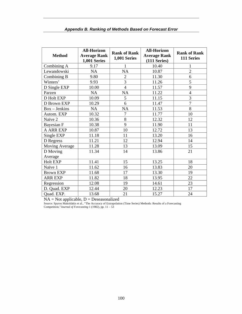
100
Appendix B. Ranking of Methods Based on Forecast Error
Method All-Horizon
Average Rank 1,001 Series
Rank of Rank 1,001 Series
All-Horizon Average Rank
(111 Series)
Rank of Rank 111 Series
Combining A 9.17 1 10.40 1 Lewandowski NA NA 10.87 2 Combining B 9.80 2 11.30 6 Winters’ 9.93 3 11.26 5 D Single EXP 10.00 4 11.57 9 Parzen NA NA 11.22 4 D Holt EXP 10.09 5 11.15 3 D Brown EXP 10.29 6 11.47 7 Box – Jenkins NA NA 11.53 8 Autom. EXP 10.32 7 11.77 10 Naïve 2 10.36 8 12.32 12 Bayesian F 10.38 9 11.90 11 A ARR EXP 10.87 10 12.72 13 Single EXP 11.18 11 13.20 16 D Regress 11.21 12 12.94 14 Moving Average 11.28 13 13.09 15 D Moving Average
11.34 14 13.86 21
Holt EXP 11.41 15 13.25 18 Naïve 1 11.62 16 13.83 20 Brown EXP 11.68 17 13.30 19 ARR EXP 11.82 18 13.95 22 Regression 12.08 19 14.61 23 D. Quad. EXP 12.44 20 12.23 17 Quad. EXP. 13.68 21 15.27 24 NA = Not applicable, D = Deseasonalized Source: Spyros Makridakis et al., “The Accuracy of Extrapolation (Time Series) Methods: Results of a Forecasting Competition,”Journal of Forecasting 1 (1982), pp. 11 – 53
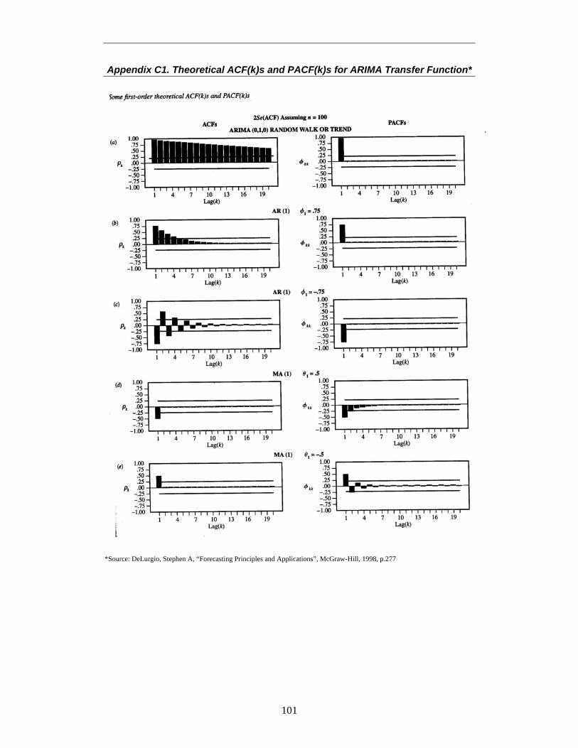
101
Appendix C1. Theoretical ACF(k)s and PACF(k)s for ARIMA Transfer Function* *Source: DeLurgio, Stephen A, “Forecasting Principles and Applications”, McGraw-Hill, 1998, p.277
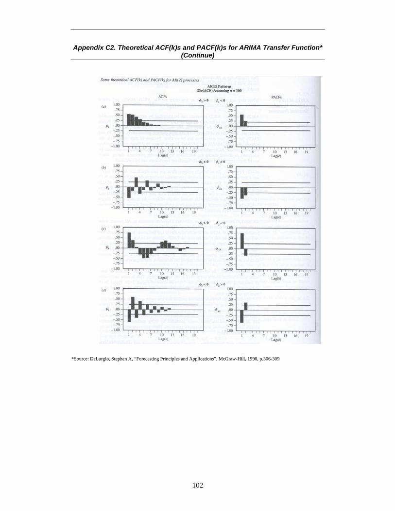
102
Appendix C2. Theoretical ACF(k)s and PACF(k)s for ARIMA Transfer Function* (Continue)
*Source: DeLurgio, Stephen A, “Forecasting Principles and Applications”, McGraw-Hill, 1998, p.306-309

103
Appendix C3. Theoretical ACF(k)s and PACF(k)s for ARIMA Transfer Function* (Continue)
*Source: DeLurgio, Stephen A, “Forecasting Principles and Applications”, McGraw-Hill, 1998, p.306-309

104
Appendix C4. Theoretical ACF(k)s and PACF(k)s for ARIMA Transfer Function* (Continue)
*Source: DeLurgio, Stephen A, “Forecasting Principles and Applications”, McGraw-Hill, 1998, p.306-309

105
Appendix C5. Theoretical ACF(k)s and PACF(k)s for ARIMA Transfer Function*
(Continue) *Source: DeLurgio, Stephen A, “Forecasting Principles and Applications”, McGraw-Hill, 1998, p.306-309
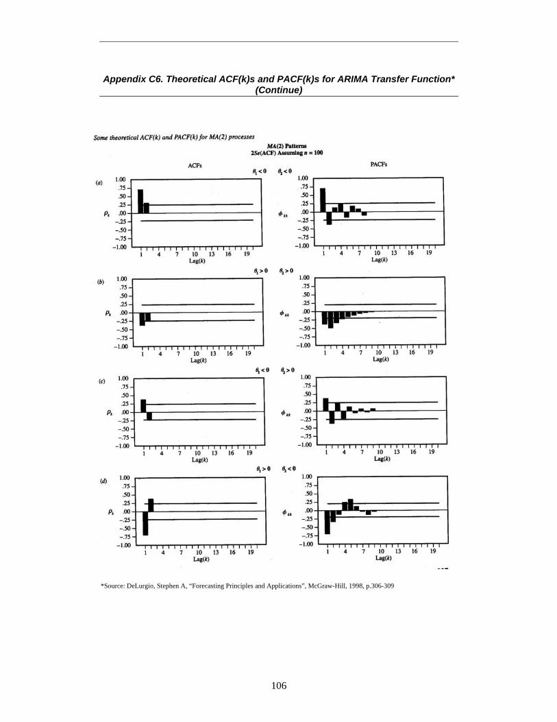
106
Appendix C6. Theoretical ACF(k)s and PACF(k)s for ARIMA Transfer Function*
(Continue) *Source: DeLurgio, Stephen A, “Forecasting Principles and Applications”, McGraw-Hill, 1998, p.306-309
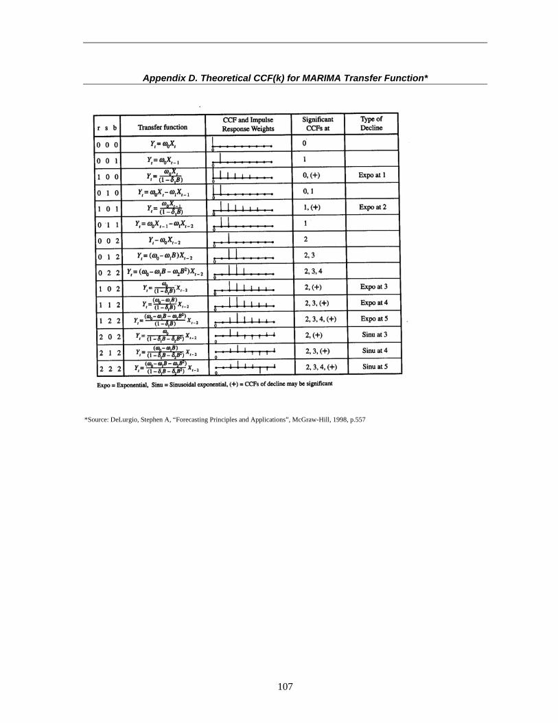
107
Appendix D. Theoretical CCF(k) for MARIMA Transfer Function*
*Source: DeLurgio, Stephen A, “Forecasting Principles and Applications”, McGraw-Hill, 1998, p.557

108
Appendix E. Formulation for System Dynamics Model Following is the list of the model equation. This list is an example of formulation in system dynamics modeling, however it has not been verified and validated due to data unavailability. The notations used for the equation is explained as follows: Init = initial condition of the level Flow = rate that changes the level position Aux = auxiliary or converters Const = constant Doc = documentation explaining the meaning and formulation of the equation Model Listing init expected_consumer_sales = consumer_sales_rate flow expected_consumer_sales = +dt*change_in_expected_sales init Inventory_level = desired_inventory flow Inventory_level = -dt*delivery_quantity_rate_vending -dt*delivery_quantity_rate_non_vending +dt*prod_quantity_rate doc Inventory_level = The level of finished goods inventory in the plant. Increased by production and decreased by deliveries. Initially set to the desired inventory level. init prod_avail_in_vending = desired_inventory_vending flow prod_avail_in_vending = -dt*consumer_demand_rate +dt*delivery_to_vending_rate init smoothed_total_order = total_order_rate flow smoothed_total_order = +dt*change_in_smoothed_order doc smoothed_total_order = The demand forecast is formed by adaptive expectations, using exponential smoothing, a common forecasting technique. The initial forecast is equal to the initial customer order rate. init trend_order = input_for_trend flow trend_order = +dt*change_in_trend_order init WIP = desired_WIP flow WIP = -dt*finish_prod_rate +dt*prod_start_rate doc WIP = WIP inventory accumulates the difference between production starts and completions. aux change_in_expected_sales = (consumer_sales_rate-expected_consumer_sales)/time_to_averge_sales_rate aux change_in_smoothed_order = (total_order_rate-smoothed_total_order)/time_to_average_order_rate doc change_in_smoothed_order = The demand forecast adjusts to the actual order rate over a time period determined by the Time to Average Order Rate. The demand forecast is formed by first-order exponential smoothing, a widely used forecasting technique.
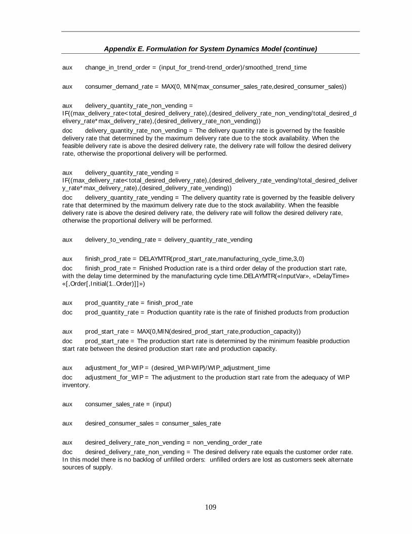
109
Appendix E. Formulation for System Dynamics Model (continue) aux change_in_trend_order = (input_for_trend-trend_order)/smoothed_trend_time aux consumer_demand_rate = MAX(0, MIN(max_consumer_sales_rate,desired_consumer_sales)) aux delivery_quantity_rate_non_vending = IF((max_delivery_rate<total_desired_delivery_rate),(desired_delivery_rate_non_vending/total_desired_delivery_rate*max_delivery_rate),(desired_delivery_rate_non_vending)) doc delivery_quantity_rate_non_vending = The delivery quantity rate is governed by the feasible delivery rate that determined by the maximum delivery rate due to the stock availability. When the feasible delivery rate is above the desired delivery rate, the delivery rate will follow the desired delivery rate, otherwise the proportional delivery will be performed. aux delivery_quantity_rate_vending = IF((max_delivery_rate<total_desired_delivery_rate),(desired_delivery_rate_vending/total_desired_delivery_rate*max_delivery_rate),(desired_delivery_rate_vending)) doc delivery_quantity_rate_vending = The delivery quantity rate is governed by the feasible delivery rate that determined by the maximum delivery rate due to the stock availability. When the feasible delivery rate is above the desired delivery rate, the delivery rate will follow the desired delivery rate, otherwise the proportional delivery will be performed. aux delivery_to_vending_rate = delivery_quantity_rate_vending aux finish_prod_rate = DELAYMTR(prod_start_rate,manufacturing_cycle_time,3,0) doc finish_prod_rate = Finished Production rate is a third order delay of the production start rate, with the delay time determined by the manufacturing cycle time.DELAYMTR(«InputVar», «DelayTime» «[,Order[,Initial(1..Order)]]») aux prod_quantity_rate = finish_prod_rate doc prod_quantity_rate = Production quantity rate is the rate of finished products from production aux prod_start_rate = MAX(0,MIN(desired_prod_start_rate,production_capacity)) doc prod_start_rate = The production start rate is determined by the minimum feasible production start rate between the desired production start rate and production capacity. aux adjustment_for_WIP = (desired_WIP-WIP)/WIP_adjustment_time doc adjustment_for_WIP = The adjustment to the production start rate from the adequacy of WIP inventory. aux consumer_sales_rate = (input) aux desired_consumer_sales = consumer_sales_rate aux desired_delivery_rate_non_vending = non_vending_order_rate doc desired_delivery_rate_non_vending = The desired delivery rate equals the customer order rate. In this model there is no backlog of unfilled orders: unfilled orders are lost as customers seek alternate sources of supply.

110
Appendix E. Formulation for System Dynamics Model (continue) aux desired_delivery_rate_vending = vending_order_rate doc desired_delivery_rate_vending = the desired delivery rate for vending customer is derived from the vending order rate. in this model, there is no backlog order. aux desired_inventory = forecast_demand*desired_inventory_coverage doc desired_inventory = The desired inventory level sought by the plant. Experience suggests that to maintain customer service by providing full and reliable deliveries, the plant must maintain a certain coverage of throughput (demand), estimated by the demand forecast. aux desired_inventory_coverage = min_order_processing_time+safety_stock_coverage doc desired_inventory_coverage = Desired inventory coverage is the number of days of the demand forecast the plant seeks to maintain in inventory. This inventory coverage is required to maintain delivery reliability by buffering the plant against unforeseen variations in demand or production. It consists of the normal order processing time plus an additional term representing the coverage desired to maintain safety stocks. aux desired_inventory_vending = expected_consumer_sales*desired_inventory_vending_coverage aux desired_inventory_vending_coverage = replenishment_cycle_time+safety_stock_vending aux desired_order_vending = MAX(0,(expected_consumer_sales+inventory_vending_adjustment)) aux desired_prod_start_rate = desired_production+adjustment_for_WIP doc desired_prod_start_rate = The desired rate of production starts, equal to the desired production rate adjusted by the adequacy of the WIP inventory. aux desired_production = MAX(0,(forecast_demand+inventory_adjustment)) doc desired_production = Desired Production is the demand forecast (Sales order forecast) adjusted to bring the inventory position in line with the target inventory level. aux desired_WIP = manufacturing_cycle_time*desired_production doc desired_WIP = The desired quantity of work in process inventory. Proportional to the manufacturing cycle time and the desired rate of production. aux forecast_demand = (smoothed_total_order+(trend_order*future_time))*seasonality aux input_for_trend = change_in_smoothed_order aux inventory_adjustment = (desired_inventory-Inventory_level)/inventory_adjustment_time doc inventory_adjustment = The desired production rate is adjusted above or below the forecast based on the inventory position of the plant. When desired inventory > inventory, desired production is increased (and vice-versa). Inventory gaps are corrected over the inventory adjustment time. aux inventory_vending_adjustment = (desired_inventory_vending-prod_avail_in_vending)/replenishment_cycle_time aux max_consumer_sales_rate = prod_avail_in_vending

111
Appendix E. Formulation for System Dynamics Model (continue) aux max_delivery_rate = Inventory_level/min_order_processing_time doc max_delivery_rate = The maximum rate of deliveries the company can achieve given their current inventory level and the minimum order processing time aux non_vending_order_rate = (input) doc non_vending_order_rate = the incoming order from customer non vending aux seasonality = total_order_rate/smoothed_total_order aux total_desired_delivery_rate = desired_delivery_rate_non_vending+desired_delivery_rate_vending aux total_order_rate = non_vending_order_rate+vending_order_rate doc total_order_rate = Customer order rate is exogenous. A variety of test inputs allow users to try different patterns, including a step, pulse, sine wave, and random noise. aux vending_capacity = capacity_per_vending*number_of_vending aux vending_inventory_coverage = prod_avail_in_vending/consumer_demand_rate aux vending_order_rate = MAX(0,MIN(desired_order_vending,vending_capacity)) const capacity_per_vending = (constant) const future_time = (constant) const inventory_adjustment_time = (constant) doc inventory_adjustment_time = The inventory adjustment time is the time period over which the plant seeks to bring inventory in balance with the desired level. const manufacturing_cycle_time = (constant) doc manufacturing_cycle_time = The average delay between the start and completion of production const min_order_processing_time = (constant) doc min_order_processing_time = The minimum time required to process and ship an order, start from the company receive the order until the order is shipped const number_of_vending = (constant) const production_capacity = (constant) const replenishment_cycle_time = (constant) const safety_stock_coverage = (constant)

112
Appendix E. Formulation for System Dynamics Model (continue) doc safety_stock_coverage = Safety stock coverage is the number of days of the expected order rate the company would like to maintain in inventory over and above the normal order processing time. The safety stock provides a buffer against the possibility that unforeseen variations in demand will cause deliveries to fall below orders. const safety_stock_vending = (constant) const smoothed_trend_time = (constant) const time_to_average_order_rate = (constant) doc time_to_average_order_rate = The demand forecast adjusts to actual customer orders over this time period. const time_to_averge_sales_rate = (constant) const WIP_adjustment_time = (constant) doc WIP_adjustment_time = The time required to adjust the WIP inventory to the desired level.

113
Appendix F1. Example Calculation of Winters Exponential Smoothing* Smoothed Trend Seasonal
Period Actual Value (Xt)
St Tt St+Tt It Forecast (Ft)
Error (et) ABS et % et ABS % et
(1) (2) (3) (4) (5) (6) (7) (8) (9) (10) (11)
1 546 652.958 0.836 2 578 660.875 0.875 3 660 668.792 0.987 4 707 676.708 1.045 5 738 684.625 1.078 6 781 692.542 1.128 7 848 700.458 1.211 8 818 708.375 1.155 9 729 716.292 1.018
10 691 724.208 0.954 11 658 732.125 0.899 12 604 740.042 7.917 740.042 0.816 13 629 749.344 7.980 757.324 0.839 625.438 3.562 3.562 0.566 0.56614 711 775.414 8.813 784.226 0.906 662.354 48.646 48.646 6.842 6.84215 729 769.423 8.132 777.555 0.957 773.917 -44.917 44.917 -6.161 6.16116 789 770.283 7.797 778.080 1.029 812.361 -23.361 23.361 -2.961 2.96117 861 784.796 8.106 792.902 1.092 838.741 22.259 22.259 2.585 2.58518 903 795.445 8.223 803.669 1.133 894.179 8.821 8.821 0.977 0.97719 968 802.339 8.162 810.501 1.208 972.950 -4.950 4.950 -0.511 0.51120 894 798.691 7.619 806.310 1.128 935.930 -41.930 41.930 -4.690 4.69021 860 818.896 8.198 827.093 1.042 820.615 39.385 39.385 4.580 4.58022 792 828.059 8.242 836.301 0.956 789.167 2.833 2.833 0.358 0.35823 739 831.731 8.032 839.763 0.891 751.628 -12.628 12.628 -1.709 1.70924 699 845.186 8.281 853.468 0.824 685.389 13.611 13.611 1.947 1.94725 773 875.684 9.303 884.988 0.872 715.715 57.285 57.285 7.411 7.41126 818 890.705 9.566 900.271 0.915 802.068 15.932 15.932 1.948 1.94827 871 903.371 9.709 913.080 0.962 861.875 9.125 9.125 1.048 1.04828 882 894.769 8.867 903.636 0.997 939.957 -57.957 57.957 -6.571 6.57129 959 895.287 8.482 903.770 1.076 987.039 -28.039 28.039 -2.924 2.92430 979 890.778 7.885 898.663 1.108 1024.274 -45.274 45.274 -4.624 4.62431 955 863.608 6.272 869.880 1.131 1085.151 -130.151 130.151 -13.628 13.62832 925 853.617 5.524 859.141 1.095 981.419 -56.419 56.419 -6.099 6.09933 843 842.828 4.774 847.602 1.011 895.267 -52.267 52.267 -6.200 6.20034 790 840.729 4.458 845.186 0.944 810.201 -20.201 20.201 -2.557 2.55735 746 842.584 4.338 846.922 0.887 753.129 -7.129 7.129 -0.956 0.95636 822 895.797 6.586 902.383 0.894 698.126 123.874 123.874 15.070 15.07037 857 906.459 785.842 71.158 71.158 8.303 8.30338 876 912.814 831.484 44.516 44.516 5.082 5.08239 959 919.168 879.699 79.301 79.301 8.269 8.26940 981 925.523 918.14 62.860 62.860 6.408 6.40841 1051 931.877 995.507 55.493 55.493 5.280 5.28042 1124 938.232 1030.497 93.503 93.503 8.319 8.31943 1073 944.586 1057.455 15.545 15.545 1.449 1.44944 1020 950.941 1029.654 -9.654 9.654 -0.946 0.94645 933 957.295 957.302 -24.302 24.302 -2.605 2.60546 787 963.650 900.525 -113.525 113.525 -14.425 14.42547 830 970.004 852.434 -22.434 22.434 -2.703 2.70348 922 976.359 869.003 52.997 52.997 5.748 5.748
Fitted Values Periods 13-36 Forecasted Values Periods 37-48 average Yt (12 month) 696.50Mean Error -7.495 Mean Error 25.455 average trend (3 years) 7.917MAD 36.273 MAD 53.774 alpha 0.33MAPE 4.288 MAPE 5.795 beta 0.05RSE 50.2593 RSE 64.8303 gamma 0.75
*Source: DeLurgio, Stephen A, “Forecasting Principles and Applications”, McGraw-Hill, 1998, p.227

114
Appendix F2. Example Chart of Winters Exponential Smoothing* *Source: DeLurgio, Stephen A, “Forecasting Principles and Applications”, McGraw-Hill, 1998, p.228
Winters Exponential Smoothing
0
200
400
600
800
1000
1200
1 3 5 7 9 11 13 15 17 19 21 23 25 27 29 31 33 35 37 39 41 43 45 47
Period
Qua
ntity Actual Value
Forecast Value

115
Appendix G. Example Calculation of ARIMA Model*
Figure G1. Demand for Animal Pharmaceutical Figure G2. ACF(s) graph of Demand for Animal Pharmaceutical (DAP) Table G1. ACF(s) and PACF(s) for Animal Pharmaceutical
Figure G3. PACF(s) graph for DAP Table G2. Seasonal ARIMA Model and Trends Table G3. Statistics Test Results of ARIMA, 1(0,1,0)12 model of DAP
Consider the following seasonal model: (1-B)(1- B12)Yt = et This very general model is easily interpreted after expansion as follow: Yt = Yt-12 + (Yt-1 – Yt-13) + et The term (Yt-1 – Yt-13) represents a stochastic trend of how much Yt-1 is higher or lower than Yt-
13. Therefore, it could be modeled by a deterministic trend coefficient of θ0. The model becomes: Yt = Yt-12 +θ0 + et
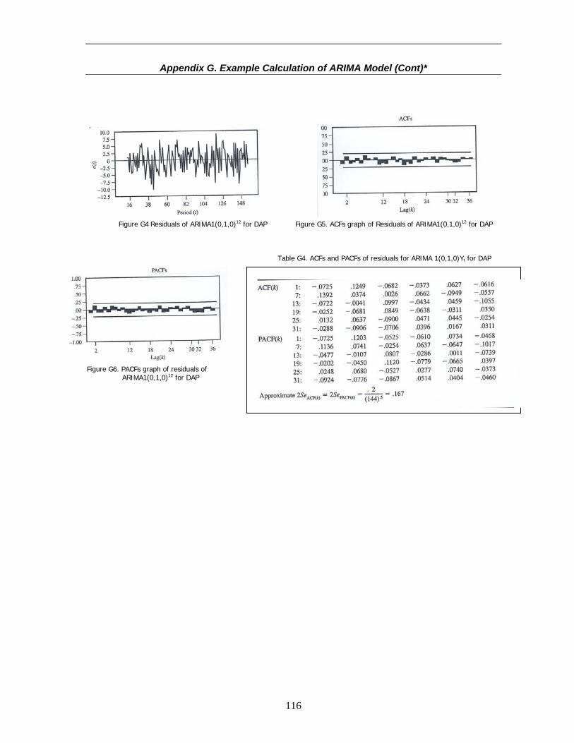
116
Appendix G. Example Calculation of ARIMA Model (Cont)*
Figure G4 Residuals of ARIMA1(0,1,0)12 for DAP Figure G5. ACFs graph of Residuals of ARIMA1(0,1,0)12 for DAP Table G4. ACFs and PACFs of residuals for ARIMA 1(0,1,0)Yt for DAP Figure G6. PACFs graph of residuals of ARIMA1(0,1,0)12 for DAP

117
Appendix H. Example Calculation of MARIMA Model* Figure H1. Market Share, Advertising Ratio and Price Ratio Table H1. Cross Correlation of β1t and α1t-k Of Auto Manufacturer Table H2. Cross Correlation between
et of equation (ex2-6) and α1t-k Table H3. Cross Correlation of β2t and α2t-k Table H4. ACFs and PACFs of et of equation ex2-11 using equation ex2-10 Table H5. Cross Correlation of et and α2t-k of equation ex2-11 Table H6. Cross Correlation of et and α2t-k for
equation ex2-13
Table H9. Cross Correlation of et and α2t-k Table H10. ACFs and PACFs of et of for equation ex2-15 equation ex2-15

118
Appendix H. Example Calculation of MARIMA Model (Cont)* Table H8. Statistics Tests Results of MARIMA Table H7. BIC Calculation for
(equation ex2-17) Equation ex2-13 and ex2-15
Table H11. ACFs and PACFs of Equation ex2-17 Table H12. Statistics Tests Results of MARIMA
(equation ex2-18) Table H13. CCFs of et and α2t-k for equation ex2-18
Table H14. CCFs of et and α1t-k for equation ex2-18
BIC (Bayesian Information Criterion) Calculation: BIC = nLn(SSE) + kLn(n) Where: n = number of observation SSE = Sum of Squared Errors k = number of coefficients estimated BIC (equation ex2-13) = 98Ln(47.97) + 2Ln(98) = 388.49 BIC (equation ex2-15) = 97Ln(40.61) + 3Ln(97) = 373.01