forecasting and oracle efficient...
TRANSCRIPT

Forecasting and Oracle EfficientEconometrics
By Anders Bredahl Kock
A dissertation submitted to
Business and Social Sciences, Aarhus University,
in partial fulfilment of the requirements of
the PhD degree in
Economics and Management
CREATESCenter for Research in Econometric Analysis of Time Series


i
Preface
This thesis was written in the period September 2007-August 2011 during mygraduate studies at the School of Economics and Management at Aarhus Univer-sity and the Department of Economics at the University of California, Berkeley.I would like to thank both of these institutions for providing me with stimulatingresearch environments. I am grateful to the Danish National Research Founda-tion for funding the Center for Research in the Econometric Analysis of TimeSeries (CREATES) and hence my PhD studies. This has given me the oportunityto travel to and present my work at several conferences across the world.
I would also like to thank two my supervisors, Niels Haldrup and TimoTerasvirta. I would like to thank Niels for encouraging me to write a PhD the-sis already when he supervised my bachelor thesis and for always providing mewith support and guidance. I am grateful to Timo for letting me work with himon three different papers – one of which can be found in this thesis and for al-ways providing me with unbelievably detailed feedback on my work. I look verymuch forward to continuing this collaboration.
I am grateful to Michael Jansson for inviting me to visit UC Berkeley. Ienjoyed the inspiring research environments and courses at the Departments ofEconomics and Statistics very much. Special thanks also to Svend Erik Gra-versen for teaching me probability theory and even spending his free time doingso. His rigor and attention to detail is something I will strive to live up to. Thevalue of his enthusiastic help and teaching can not be overestimated for Chapter3 and will also be of much use in my future career.
I would also like to thank all my friends at the International House in Berke-ley for making my stay there an unforgettable experience and for giving me thechance to meet wonderful people from all over the world.
At the School of Economics and Management I would like to thank my fel-low PhD students for providing me with a very pleasant evironment with heapsof fun. I also appreciate your patience with me in my less productive moments.Thanks to Malene for trying to raise me and to Johannes and Stefan for help-ing me with LATEX-related problems. Thomas, Kajetan and Anders deserve mygratitude for sharing an office with me and bearing over with my messy desk.Kenneth and Christian deserve thanks for having supported me all the way fromthe beginning of our joint studies at university in 2003. Finally, I would like tothank Anne, Lasse, Laurent, Mikkel, Niels H/S and all the other PhD studentsfor many funny hours.

ii
I would like to thank my parents, Anette and Hans, my brother Henrik, andmy aunt Gitte for always being curious and supportive about my endeavours andwork.
Anders Bredahl Kock, Aarhus, August 2011
Updated prefaceThe predefense was held on Monday, October 17th, 2011. I would like to thankthe committee consisting of Henning Bunzel, Dick van Dijk and Jurgen Doornikfor their careful reading and constructive comments. In particular, I appreciatethe numerous suggestions pointing me towards future avenues of research.
Anders Bredahl Kock, Aarhus, November 2011

Contents
Summary v
Dansk resume xv
1 Forecasting with Universal Approximators and a Learning Algo-rithm 11.1 Introduction . . . . . . . . . . . . . . . . . . . . . . . . . . . . 21.2 Universal Approximators . . . . . . . . . . . . . . . . . . . . . 41.3 Benchmark Models . . . . . . . . . . . . . . . . . . . . . . . . 81.4 Forecasting with Experts . . . . . . . . . . . . . . . . . . . . . 81.5 Application . . . . . . . . . . . . . . . . . . . . . . . . . . . . 111.6 Conclusions . . . . . . . . . . . . . . . . . . . . . . . . . . . . 221.7 Appendix . . . . . . . . . . . . . . . . . . . . . . . . . . . . . 241.8 Bibliography . . . . . . . . . . . . . . . . . . . . . . . . . . . . 31
2 Forecasting by Automated Modelling Techniques 332.1 Introduction . . . . . . . . . . . . . . . . . . . . . . . . . . . . 342.2 The Model . . . . . . . . . . . . . . . . . . . . . . . . . . . . . 372.3 Modeling with three Automatic Model Selection Algorithms . . 392.4 Forecasting . . . . . . . . . . . . . . . . . . . . . . . . . . . . 432.5 Results . . . . . . . . . . . . . . . . . . . . . . . . . . . . . . . 452.6 Conclusions . . . . . . . . . . . . . . . . . . . . . . . . . . . . 672.7 Appendix: Creating the Pool of Hidden Units . . . . . . . . . . 682.8 Bibliography . . . . . . . . . . . . . . . . . . . . . . . . . . . . 70
3 Oracle Efficient Estimation in Panels 753.1 Introduction . . . . . . . . . . . . . . . . . . . . . . . . . . . . 763.2 Setup and Assumptions . . . . . . . . . . . . . . . . . . . . . . 773.3 The Bridge estimator . . . . . . . . . . . . . . . . . . . . . . . 80
iii

iv Contents
3.4 The Marginal Bridge estimator . . . . . . . . . . . . . . . . . . 863.5 Simulations . . . . . . . . . . . . . . . . . . . . . . . . . . . . 893.6 Conclusions . . . . . . . . . . . . . . . . . . . . . . . . . . . . 943.7 Appendix . . . . . . . . . . . . . . . . . . . . . . . . . . . . . 963.8 Bibliography . . . . . . . . . . . . . . . . . . . . . . . . . . . . 116

English Summary
If it exists, the overall theme for this thesis could be called machine learning ineconometrics, i.e. trying to enable computers to learn patterns from data. Thesepatterns could be figuring out which covariates from a huge database are relevantin explaining a particular phenomenon. Having learned these covarites, one canuse these to form out of sample predictions – an extemely important topic ineconometrics. This thesis conists of three self-contained chapters dealing withvarious aspects of machine learning, forecasting, and variable selection.
In Chapter 1 we examine the forecast performance of nonlinear models com-pared to that of linear autoregressions. Linear models have the advantage thatthey can be understood and analyzed in great detail. However, it might beinappropriate to assume that the generating mechanism of a series is linear.Hence, nonlinear models have become increasingly popular, see e.g. Grangerand Terasvirta (1993) and Terasvirta, Granger, and Tjøstheim (2010). However,the nonlinear models are still restricted by the fact that modeling takes placewithin a prespecified family of models. Since the modeler often has little priorknowledge regarding the functional form of the data generating process, choos-ing the correct family is still not an easy task. If one wants to avoid making thischoice, one may apply universal approximators which are able to approximatebroad classes of functions arbitrarily well in various metrics.
The universal approximators are data driven in the sense that little a prioriknowledge is needed about the functional relationship between the left- and theright-hand side variables. Artificial Neural Networks (ANN) are a particulartype of universal approximators which have been applied in numerous forecast-ing studies such as Stock and Watson (1999a) and Terasvirta, van Dijk, andMedeiros (2005). Other universal approximators have also been studied, but inour experience no comparison of the relative forecasting performance has beenmade.
The paper has three purposes. First, a comparison of the forecast perfor-
v

vi English Summary
mance of three universal approximators is made. Second, we wish to investigatethe stability of forecasts from the universal approximators since recursive fore-casts by nonlinear models can be erratic. Third, we investigate the performanceof a forecast combination algorithm developed in the computer science litera-ture. Its main virtue is that its worst case performance can be explicitly boundedindependently of the joint distribution of forecasts combined from.
Besides the ANNs the universal approximators considered are theKolmogorov-Gabor polynomials and Elliptic Basis Function Networks (EBF).The latter nest the more well known Radial Basis Function Networks as a specialcase. All the universal approximators applied nest the linear autoregression, andwe are hence able to investigate how much (if at all) the nonlinear structureadds to the forecasting performance. While a comparison of recursive and directnonlinear forecasting procedures is of interest in its own right, we focus on theformer here. Hence standard direct procedures such as kernel regression are notconsidered.
In investigating the stability of the forecasts we are particularly interested indealing with the importance of handling insane forecasts. Here insane forecastsare to be understood as forecasts that are clearly unrealistic in the light of thehitherto observed values of the time series to be forecast. A precise definitionshall be given later. Handling insane forecasts turned out to be particularly im-portant for the Kolmogorov-Gabor polynomials since their polynomial structurecould yield explosive forecasts.
Forecast combination has a long history in econometrics. The first to studythis were Bates and Granger (1969). The literature has proliferated since then,and a recent survey is given in Timmermann (2006). Two caveats apply, how-ever, to many of these combination algorithms. First, nothing can be said a prioriabout the performance of the algorithm (combination rule) compared to the in-dividual forecasts. And even if bounds are provided, they often depend on thejoint distribution of the vector consisting of the forecasts made by the individ-ual models. The Weighted Average Algorithm (WAA) of Kivinen and Warmuth(1999) developed in the computer science literature does not share any of theseproblems. First, explicit loss bounds for the worst case performance of the algo-rithm are available. Furthermore, these bounds do not depend on the distributionof the vector of forecasts from the individual models.
We argue that forecasting with universal approximators and combining theseinto a single forecast by an algorithm for which explicit bounds can be derivedforms a solid theoretical foundation for combining forecasts. The empirical per-

vii
formance of the universal approximators as well as the WAA will be investigatedby considering various monthly postwar macroeconomic data sets for the G7 andthe Scandinavian countries.
Chapter 2 is concerned with the task of building Artificial Neural NetworkModels and using them for forecasting. It is joint work with one of my supervi-sors, Timo Terasvirta.
Artificial Neural Networks (ANN) have been quite popular in many areasof science for describing various phenomena and forecasting them. They havealso been used in forecasting macroeconomic time series and financial series,see Kuan and Liu (1995) for a successful example on exchange rate forecasting,and Zhang, Patuwo, and Hu (1998) and Rech (2002) for more mixed results.The main argument in their favour is that ANNs are universal approximators,which means that they are capable of approximating arbitrarily accurately func-tions satisfying only mild regularity conditions. The ANN models thus have astrong nonparametric flavour. One may therefore expect them to be a versatiletool in economic forecasting and adapt quickly to rapidly changing forecastingsituations. Recently, Ahmed, Atiya, El Gayer, and El-Shishiny (2010) conductedan extensive forecasting study comprising more than 1000 economic time seriesfrom the M3 competition Makridakis and Hibon (2000), and a large number ofwhat they called machine learning tools. They concluded that the ANN modelthat we are going to consider, the single hidden-layer feedforward ANN modelor multi-layer perceptron with one hidden layer, was one of the best or even thebest performer in their study. A single hidden-layer ANN model is already a uni-versal approximator; see Cybenko (1989) and Hornik, Stinchcombe, and White(1989).
A major problem in the application of ANN models is the specification andestimation of these models. A large number of modelling strategies have beendeveloped for the purpose. It is possible to begin with a small model and increaseits size (“specific-to-general”, “bottom up”, or “growing the network”). Con-versely, one can specify a network with a large number of variables and hiddenunits or “neurons” and then reduce its size (“general-to-specific”, “top down” or“pruning the network”). Since the ANN model is nonlinear in parameters, itsparameters have to be estimated numerically, which may be a demanding task ifthe number of parameters in the model is large. Recently, White (2006) deviseda clever strategy for modelling ANNs that converts the specification and ensuingnonlinear estimation problem into a linear model selection problem. This greatlysimplifies the estimation stage and alleviates the computational effort. It is there-

viii English Summary
fore of interest to investigate how well this strategy performs in macroeconomicforecasting. A natural benchmark in that case is a linear autoregressive model.
Quite often, application of White’s strategy leads to a situation in whichthe number of variables in the set of candidate variables exceeds the numberof observations. The strategy handles these cases without problems, because itessentially works from specific to general and then back again. We shall alsoconsider a one-way variant from specific to general in this study. One may wantto set a maximum limit for variables to be included in the model to control itssize.
There exist other modelling strategies that can also be applied to selecting thevariables. In fact, White (2006) encouraged comparisons between his methodand other alternatives, and here we shall follow his suggestion. In this work, weconsider two additional specification techniques. One is Autometrics by Doornik(2009), see also Krolzig and Hendry (2001) and Hendry and Krolzig (2005), andthe other one is the Marginal Bridge Estimator (MBE), see Huang, Horowitz,and Ma (2008b). The former is designed for econometric modelling, whereasthe latter one has its origins in statistics. Autometrics works from general to spe-cific, and the same may be said about MBE. We shall compare the performanceof these three methods when applying White’s idea of converting the specifica-tion and estimation problem into a linear model selection problem and selectinghidden units for our ANN models. That is one of the main objectives of thispaper.
The focus in this study is on multiperiod forecasting. There are two waysof generating multiperiod forecasts. One consists of building a single modeland generating the forecasts for more than one period ahead recursively. Theother one, called direct forecasting, implies that a separate model is built foreach forecasting horizons, and no recursions are involved. For discussion, seefor example Terasvirta (2006), Terasvirta et al. (2010, Chapter 14), or Kock andTerasvirta (2011). In nonlinear forecasting, the latter method appears to be morecommon, see for example Stock and Watson (1999b) and Marcellino (2002),whereas Terasvirta, van Dijk, and Medeiros (2005) constitutes an example ofthe former alternative. A systematic comparison of the performance of the twomethods exists, see Marcellino, Stock, and Watson (2006), but it is restricted tolinear autoregressive models. Our aim is to extend these comparisons to nonlin-ear ANN models.
Nonlinear models can sometimes generate obviously insane forecasts. Oneway of alleviating this problem is to use insanity filters as in Swanson and White

ix
(1995, 1997a,b) who discuss this issue. We will compare two filters to the un-filtered forecasts and see how they impact on the forecasting performance of theneural networks.
In this work the ANN models are augmented by including lags of the vari-able to be forecast linearly in them. As a result, the augmented models nest alinear autoregressive model. It is well known that if the data-generating processis linear, the augmented ANN model is not even locally identified; see for ex-ample Lee, White, and Granger (1993), Terasvirta, Lin, and Granger (1993) orTerasvirta et al. (2010, Chapter 5) for discussion. A general discussion of iden-tification problems in ANN models can be found in Hwang and Ding (1997). Itmay then be advisable to first test linearity of each series under consideration be-fore applying any ANN modelling strategy to it. But then, it may also be arguedthat linearity tests are unnecessary, because the set of candidate variables can be(and in our case is) defined to include both linear lags and hidden units. Themodelling technique can then choose among all of them and find the combina-tion that is superior to the others. We shall compare these two arguments. Thisis done by carrying out pretesting and only fitting an ANN model to the series iflinearity is rejected. Forecasts are generated from models specified this way andcompared with forecasts from the ANN models obtained using White’s methodand the three automatic modelling techniques.
The main criterion of comparing forecasts is the Root Mean Square ForecastError (RMSFE), which implies a quadratic loss function. Other alternatives arepossible, but the RMSFE is commonly used and thus even applied here. We rankthe methods, which makes some comparisons possible. Furthermore, we alsocarry out Wilcoxon signed rank tests but principally for descriptive purposes, sothe tests are not used as an ex post model selection criterion; see Costantini andKunst (2011) for a discussion.
It might be desirable to compare White’s method with modelling strategieswhich are not based on linearising the problem but in which statistical methodssuch as hypothesis testing and nonlinear maximum likelihood estimation are ap-plied. Examples of these include Swanson and White (1995, 1997a,b), Andersand Korn (1999) and Medeiros, Terasvirta, and Rech (2006). These approachesdo, however, require plenty of human resources, unless the number of time se-ries under consideration and forecasts generated from them are small. This isbecause nonlinear iterative estimation cannot be automated and the algorithmsleft to their own devices. Each estimation needs a nonnegligible amount of ten-der loving care, and when the number of time series to be considered is large,

x English Summary
ANN model building and forecasting tend to require a substantial amount ofresources.
In this paper we investigate the forecasting performance of the above tech-niques. We first conduct a small simulation study to see how well these tech-niques perform when the data are generated by a known nonlinear model. Theeconomic data sets consist of the monthly unemployment and consumer priceindex series from the 1960’s until 2009.
Chapter 3 generalizes some recent results on oracle efficient variable selec-tion in cross sectional models to a panel data setting.
When building a model one of the first steps is to decide which variables toinclude. Sometimes theory can guide the researcher towards a set of potentialexplanatory variables but which variables in this set are relevant and which are tobe left out? Huang, Horowitz, and Ma (2008a) showed that the Bridge estimatoris able to discriminate between relevant and irrelevant explanatory variables in across section setting with fixed covariates whose number is allowed to increasewith the sample size. In fact, oracle efficient estimation has received quite someattention in the statistics literature in the recent years, see (among others) Zou(2006), Candes and Tao (2007), Fan and Lv (2008), and Meinshausen and Yu(2009). However, we are not aware of any similar results for panel data models.For the case of fewer explanatory variables than observations we show that theoracle efficiency of the Bridge estimator carries over to linear panel data modelswith random regressors in the random and fixed effects settings. More precisely,it suffices that either the number of cross sectional units (N) or the number ofobservations within each cross sectional unit (TN) goes to infinity in order toestablish consistency and correct elimination of irrelevant variables. To obtainthe oracle efficient asymptotic distribution (the distribution obtained by only in-cluding the relevant covariates) of the estimators of the nonzero coefficients,further restrictions are needed. In the classical setting of fixed TN and large Nthese restrictions are satisfied. Further sufficient conditions for oracle efficiencyare given. By fixing TN and the number of covariates we obtain as a corollarythat the asymptotic distribution of the estimators of the non-zero coefficients isexactly the classical fixed effects or random effects limit law.
If the set of potential explanatory variables is larger than the number of ob-servations we show that the Marginal Bridge estimator of Huang et al. (2008a)can be used to distinguish between relevant and irrelevant variables in randomand fixed effects panel data models. A partial orthogonality condition restrict-ing the dependence between the relevant and the irrelevant variables of the same

xi
type as in Huang et al. (2008a) is imposed. Furthermore, the error terms must beGaussian – a price paid for letting the covariates be random. The random covari-ates also rendered the maximum inequalities based on exponential Orlicz normsused in Huang et al. (2008a) inapplicable. However, more simple maximuminequalities in Lq spaces can still be applied but the result is that the numberof irrelevant variables must be o(Nq/2) for some q ≥ 1 (this is for fixed TN forcomparability to the known cross sectional results) as opposed to exp(o(N)) (asubexponential rate). Since q is arbitrary this still allows mN to increase at anypolynomial rate. The number of relevant variables may still be o(N1/2) (againTN is considered fixed for comparison).
Furthermore, the Marginal Bridge estimator is very fast to implement whichalso makes it useful as an initial screening device to weed out the most irrelevantvariables before initiating the actual modeling stage.
Since cross section data can be viewed as panel data with only one observa-tion per individual, all our results are also valid for cross section data and hencegeneralize the results for these.
Bibliography
Ahmed, N. K., A. F. Atiya, N. El Gayer, and H. El-Shishiny (2010). An empiricalcomparison of machine learning tools for time series forecasting. EconometricReviews 29, 594–621.
Anders, U. and O. Korn (1999). Model selection in neural networks. NeuralNetworks 12, 309–323.
Bates, J. and C. Granger (1969). Combination of forecasts . Operations ResearchQuarterly 20(4), 451–468.
Candes, E. and T. Tao (2007). The Dantzig selector: statistical estimation whenp is much larger than n. Annals of Statistics 35(6), 2313–2351.
Costantini, M. and R. M. Kunst (2011). On the usefulness of the Diebold-Mariano test in the selection of prediction models: some Monte Carlo evi-dence. Working paper, University of Vienna.
Cybenko, G. (1989). Approximation by superpositions of a sigmoidal function.Mathematics of Control, Signals, and Systems 2, 303–314.

xii English Summary
Doornik, J. A. (2009). Autometrics. In J. L. Castle and N. Shephard (Eds.), TheMethodology and Practice of Econometrics, pp. 88–122. Oxford UniversityPress, Oxford.
Fan, J. and J. Lv (2008). Sure independence screening for ultrahigh dimensionalfeature space. Journal of the Royal Statistical Society: Series B (StatisticalMethodology) 70(5), 849–911.
Granger, C. W. J. and T. Terasvirta (1993). Modelling Nonlinear EconomicRelationships. Oxford University Press, USA.
Hendry, D. F. and H. M. Krolzig (2005). The properties of automatic Gets mod-elling. Economic Journal 115, 32–61.
Hornik, K., M. Stinchcombe, and H. White (1989). Multilayer feedforwardnetworks are universal approximators. Neural Networks 2, 359–366.
Huang, J., J. Horowitz, and S. Ma (2008a). Asymptotic properties of bridgeestimators in sparse high-dimensional regression models. Annals of Statis-tics 36(2), 587–613.
Huang, J., J. L. Horowitz, and S. Ma (2008b). Asymptotic properties of bridgeestimators in sparse high-dimensional regression models. Annals of Statis-tics 36, 587–613.
Hwang, J. T. G. and A. A. Ding (1997). Prediction intervals for artificial neuralnetworks. Journal of the American Statistical Association 92, 748–757.
Kivinen, J. and M. K. Warmuth (1999). Averaging Expert Predictions. In PaulFischer and Hans Ulrich Simon, editors, Proceedings of the 4th EuropeanConference on Computational Learning Theory EuroCOLT ’99, 153–167.
Kock, A. B. and T. Terasvirta (2011). Forecasting with nonlinear time seriesmodels. In M. P. Clements and D. F. Hendry (Eds.), Oxford Handbook ofEconomic Forecasting, pp. 61–87. Oxford University Press, Oxford.
Krolzig, H. M. and D. F. Hendry (2001). Computer automation of general-to-specific model selection procedures. Journal of Economic Dynamics andControl 25, 831–866.
Kuan, C.-M. and T. Liu (1995). Forecasting exchange rates using feedforwardand recurrent neural networks. Journal of Applied Econometrics 10, 347–364.

xiii
Lee, T.-H., H. White, and C. W. J. Granger (1993). Testing for neglected non-linearity in time series models: A comparison of neural network methods andalternative tests. Journal of Econometrics 56, 269–290.
Makridakis, S. and M. Hibon (2000). The M3-Competition: results, conclusionsand implications. International Journal of Forecasting 16, 451–476.
Marcellino, M. (2002). Instability and non-linearity in the EMU. DiscussionPaper No. 3312, Centre for Economic Policy Research.
Marcellino, M., J. H. Stock, and M. W. Watson (2006). A comparison of di-rect and iterated multistep AR methods for forecasting macroeconomic timeseries. Journal of Econometrics 135, 499–526.
Medeiros, M. C., T. Terasvirta, and G. Rech (2006). Building neural networkmodels for time series: A statistical approach. Journal of Forecasting 25,49–75.
Meinshausen, N. and B. Yu (2009). Lasso-type recovery of sparse representa-tions for high-dimensional data. Annals of Statistics 37(1), 246–270.
Rech, G. (2002). Forecasting with artificial neural network models. SSE/EFIWorking Paper Series in Economics and Finance 491, Stockholm School ofEconomics.
Stock, J. H. and M. W. Watson (1999a). A comparison of linear and nonlinearunivariate models for forecasting macroeconomic time series, in R.F. Engleand H. White (eds). Oxford: Oxford University Press.
Stock, J. H. and M. W. Watson (1999b). A comparison of linear and nonlinearunivariate models for forecasting macroeconomic time series. In R. F. Engleand H. White (Eds.), Cointegration, Causality, and Forecasting: A Festschriftin Honour of Clive W.J. Granger, pp. 1–44. Oxford University Press, Oxford.
Swanson, N. R. and H. White (1995). A model-selection approach to assessingthe information in the term structure using linear models and artificial neuralnetworks. Journal of Business & Economic Statistics 13, 265–275.
Swanson, N. R. and H. White (1997a). A model selection approach to real-timemacroeconomic forecasting using linear models and artificial neural networks.Review of Economics and Statistics 79, 540–550.

xiv English Summary
Swanson, N. R. and H. White (1997b). Forecasting economic time series us-ing flexible versus fixed specification and linear versus nonlinear econometricmodels. International Journal of Forecasting 13, 439–461.
Terasvirta, T. (2006). Forecasting economic variables with nonlinear models.In G. Elliott, C. W. J. Granger, and A. Timmermann (Eds.), Handbook ofEconomic Forecasting, Volume 1, pp. 413–457. Elsevier, North-Holland.
Terasvirta, T., C. W. J. Granger, and D. Tjøstheim (2010). Modelling NonlinearEconomic Time Series. Oxford University Press, Oxford.
Terasvirta, T., C. F. Lin, and C. W. J. Granger (1993). Power of the neuralnetwork linearity test. Journal of Time Series Analysis 14, 209–220.
Terasvirta, T., D. van Dijk, and M. C. Medeiros (2005). Linear models, smoothtransition autoregressions, and neural networks for forecasting macroeco-nomic time series: A re-examination. International Journal of Forecast-ing 21(4), 755–774.
Terasvirta, T., D. van Dijk, and M. C. Medeiros (2005). Linear models, smoothtransition autoregressions, and neural networks for forecasting macroeco-nomic time series: A re-examination. International Journal of Forecasting 21,755–774.
Timmermann, A. (2006). Forecast Combination, in G. Elliott, C.W.J. Granger,A Timmermann (eds). Handbook of Economic Forecasting 1, 135–196.
White, H. (2006). Approximate nonlinear forecasting methods. In G. Elliott,C. W. J. Granger, and A. Timmermann (Eds.), Handbook of Economic Fore-casting, Volume 1, pp. 459–512. Elsevier, Amsterdam.
Zhang, G., B. E. Patuwo, and M. Y. Hu (1998). Forecasting with artificial neuralnetworks: The state of the art. International Journal of Forecasting 14, 35–62.
Zou, H. (2006). The adaptive lasso and its oracle properties. Journal of theAmerican Statistical Association 101(476), 1418–1429.

Dansk resume
Dansk resume (Danish summary)
Om den findes, sa er den røde trad i denne afhandling anvendelsen af teknikkerfra maskinlæring til at finde mønstre og information i økonomisk data. De sen-este ar har fremvist en stor vækst i store datasæt, og et oplagt spørgsmal er i denforbindelse, hvordan man finder frem til den ønskede information i data udenat blive overdøvet af støj. At finde frem til de variable, der faktisk driver denproces man er interesseret i, er af stor betydning, nar man laver forecasts affremtidige økonomiske variable. Denne afhandling beskæftiger sig med, hvor-dan man finder frem til de relevante forklarende variable i meget store datasæt.Vi beskriver ogsa flere metoder til at forecaste økonomiske variable pa.
Kapitel 1 har titlen ”Forecasting with Universal Approximators and a Learn-ing Algorithm” og omhandler forecasting i situationer, hvor man ikke er vil-lig til at gøre sig særlige antagelser om den datagenererende proces. Til detteformal benytter vi os af mængder af funktioner, der ligger tæt i diverse størrefunktionsrum. Ofte kaldes disse tætte mængder af funktioner for universelleapproksimatorer, da de netop har den egenskab at de kan approksimere bredeklasser af funktioner til en vilkarlig grad (de ligger tæt i dem). Kapitlet har treformal, hvoraf det første er at sammenligne præcisionen af neurale netværk, el-liptiske basisfunktionsnetværk samt Kolmogorov-Gabor-polynomier som alle eruniverselle approksimatorer. For det andet undersøges stabiliteten af forecastsmed universelle approksimatorer, idet disse kan have en tendens til at være ek-splosive. Endeligt sammenlignes forskellige mader at kombinere forecasts pa.Specielt er vi interesseret i ”The Weighted Average Algorithm”, da denne palangt sigt beviseligt ikke vil klare sig darligere end den bedste af de modellerfra den mængde af modeller man kombinerer fra. Sa selvom vi ikke ved hvilkenmodel, der er den bedste, kan vi klare os lige sa godt pa langt sigt som om vikendte den.
xv

xvi Dansk resume
Vi finder, at de elliptiske basisfunktionsnetværk er de mest præcise af de uni-verselle approksimatorer, samt at det er nødvendigt at filtrere for vilde forecastsbort, hvis man ønsker en bare nogenlunde hæderlig præcision. Endeligt er det engod ide at kombinere forecasts, men the Weighted Average Algorithm klarer sigikke meget bedre end mere simple kombinationsskemaer sa som ligelig vægnt-ing.
Kaptitel 2, ”Forecasting Macroconomic Variables using Neural NetworkModels and Three Automated Model Selection Techniques”, er skrevet sam-men med den ene af mine vejledere, Timo Terasvirta. Dette kapitel gar merei dybden med en af de universelle approksimatorer fra Kapitel 1, nemlig deneurale netværk. Disse er ikke lette at estimere, og vi benytter et snedigt lin-eariseringstrick til at gøre dette. Efter denne linearisering har fundet sted, skalvi dog vælge mellem en lang række af potentielle variable. Der er altsa taleom et højdimensioalt variabelselektionsproblem og vi sammenligner, hvordanQuickNet, Marginal Bridge estimatoren og Autometrics klarer sig i forecas-thenseende med hensyn til at vælge variable. Oftest forecaster man enten direkteeller rekursivt og vi kender ikke til nogen sammenligninger af disse metoder forikke-lineære modeller. Vi udfylder dette hul i litteraturen ved at sammenligne di-rekte og rekursive forecasts for neurale netværk. Ligesom i kapitel 1 undersøgervi forskellige mader at handtere vilde forecasts pa. Endeligt undersøger vi, omdet kan betale sig at teste for linearitet før man bygger en ikke-lineær model.
Vi finder, at Marginal Bridge estimatoren er bedst til at estimere de neuralenetværk, samt at direkte forecast ofte er mere præcise end rekursive forecasts.Det lader ikke til at det at teste linearitetshypotesen før vi bygger en ikke-lineærmodel resulterer i mere præcise forecasts. Dette kan dog skyldes, at alle voresikke-lineære modeller indeholder en lineær model som ægte delmængde.
Tredje kapitel omhandler variabelselektion i højdimensionale modeller, dvsmodeller hvor antallet af variable tillades at vokse i stikprøvestørrelsen og po-tentielt overstiger denne. Dette emne har faet meget opmærksomhed i de senestear i statistiklittereaturen. Vi bidrager til denne ved at udvide resultater for Bridgeog Marginal Bridge estimatorerne fra cross section modeller til panel data mod-eller. Specielt viser vi, at Bridge estimatoren er orakelefficient. Det vil sige atden korrekt kan skelne mellem relevante og irrelevante variable og kun beholderde relevante variable i modellen. Ydermere er den asymptotiske fordeling forkoefficienterne hørende til de relevante variable den samme som om man frastarten af kun havde inkluderet de relevante variable. Vi kan altsa opna sammeasymptotiske efficiens som om et orakel havde fortalt os, hvad den sande model

xvii
er.Ovenstaende resultater er for tilfældet, hvor der er færre variable end obser-
vationer. I tilfældet med flere variable end observationer viser vi at MarginalBridge estimatoren stadig kan skelne mellem relevante og irrelevante variable.Dog estimeres koefficienterne til de relevante variable ikke længere konsistent,og vi forreslar derfor en totrinprocedure, hvor man i første trin vælger de rele-vante forklarende variable ved hjælp af Marginal Bridge estimatoren og i andettrin estimerer koefficienterne til de relevante variable med en vilarlig konsistentestimator sasom OLS eller Bridge estimatoren. Endeligt viser vi ved simula-tioner, at de foreslaede estimatorer klarer sig godt i endelige stikprøver.


Chapter 1
Forecasting with UniversalApproximators and a LearningAlgorithm
Anders Bredahl KockAarhus University and CREATES
Journal of Time Series Econometrics (2011), Vol. 3: Iss. 3, Article 3
AbstractThis paper applies three universal approximators for forecasting. They are theArtificial Neural Networks, the Kolmogorov-Gabor polynomials, as well as theElliptic Basis Function Networks. We are particularly interested in the relativeperformance and stability of these. Even though forecast combination has a longhistory in econometrics focus has not been on proving loss bounds for the com-bination rules applied. We apply the Weighted Average Algorithm (WAA) ofKivinen and Warmuth (1999) for which such loss bounds exist. Specifically,one can bound the worst case performance of the WAA compared to the per-formance of the best single model in the set of models combined from. The
Financial support from the Center for Research in the Econometric Analysis of Time Se-ries, CREATES funded by the Danish National Research Foundation is gratefully acknowledgedby the author. The author also wishes to thank Niels Haldrup, Peter Reinhard Hansen, TimoTerasvirta, and an anonymous referee for helpful comments. Finally, the author would like tothank his PhD committee consisting of Henning Bunzel, Dick van Dijk and Jurgen Doornik fortheir careful reading and constructive comments.
1

2 Chapter 1. Forecasting with Universal Approximators and a Learning Algorithm
use of universal approximators along with a combination scheme for which ex-plicit loss bounds exist should give a solid theoretical foundation to the way theforecasts are performed. The practical performance will be investigated by con-sidering various monthly postwar macroeconomic data sets for the G7 as well asthe Scandinavian countries.
1.1 IntroductionIn this paper we examine the forecast performance of nonlinear models com-pared to that of linear autoregressions. Linear models have the advantage thatthey can be understood and analyzed in great detail. However, it might beinappropriate to assume that the generating mechanism of a series is linear.Hence, nonlinear models have become increasingly popular, see e.g. Grangerand Terasvirta (1993) and Terasvirta et al. (2010). However, the nonlinear mod-els are still restricted by the fact that modeling takes place within a prespecifiedfamily of models. Since the modeler often has little prior knowledge regardingthe functional form of the data generating process, choosing the correct fam-ily is still not an easy task. If one wants to avoid making this choice, one mayapply universal approximators which are able to approximate broad classes offunctions arbitrarily well in a way to be made clear in Section 1.2.
The universal approximators are data driven in the sense that little a prioriknowledge is needed about the functional relationship between the left- and theright-hand side variables. Artificial Neural Networks (ANN) are a particulartype of universal approximators which have been applied in numerous forecast-ing studies such as Stock and Watson (1999) and Terasvirta et al. (2005). Otheruniversal approximators have also been studied, but in our experience no com-parison of the relative forecasting performance has been made.
The paper has three purposes. First, a comparison of the forecast perfor-mance of three universal approximators is made. Second, we wish to investigatethe stability of forecasts from the universal approximators since recursive fore-casts by nonlinear models can be erratic. Third, we investigate the performanceof a forecast combination algorithm developed in the computer science litera-ture. Its main virtue is that its worst case performance can be explicitly boundedindependently of the joint distribution of forecasts combined from.
Besides the ANNs the universal approximators considered are theKolmogorov-Gabor polynomials and Elliptic Basis Function Networks (EBF).The latter nest the more well known Radial Basis Function Networks as a special

1.1. Introduction 3
case. All the universal approximators applied nest the linear autoregression, andwe are hence able to investigate how much (if at all) the nonlinear structureadds to the forecasting performance. While a comparison of recursive and directnonlinear forecasting procedures is of interest in its own right, we focus on theformer here. Hence standard direct procedures such as kernel regression are notconsidered.
In investigating the stability of the forecasts we are particularly interested indealing with the importance of handling insane forecasts. Here insane forecastsare to be understood as forecasts that are clearly unrealistic in the light of thehitherto observed values of the time series to be forecast. A precise definitionshall be given later. Handling insane forecasts turned out to be particularly im-portant for the Kolmogorov-Gabor polynomials since their polynomial structurecould yield explosive forecasts.
Forecast combination has a long history in econometrics. The first to studythis were Bates and Granger (1969). The literature has proliferated since then,and a recent survey is given in Timmermann (2006). Two caveats apply, how-ever, to many of these combination algorithms. First, nothing can be said a prioriabout the performance of the algorithm (combination rule) compared to the in-dividual forecasts. And even if bounds are provided, they often depend on thejoint distribution of the vector consisting of the forecasts made by the individ-ual models. The Weighted Average Algorithm (WAA) of Kivinen and Warmuth(1999) developed in the computer science literature does not share any of theseproblems. First, explicit loss bounds for the worst case performance of the algo-rithm are available. Furthermore, these bounds do not depend on the distributionof the vector of forecasts from the individual models.
We argue that forecasting with universal approximators and combining theseinto a single forecast by an algorithm for which explicit bounds can be derivedforms a solid theoretical foundation for combining forecasts. The empirical per-formance of the universal approximators as well as the WAA will be investigatedby considering various monthly postwar macroeconomic data sets for the G7 andthe Scandinavian countries.
The outline of the paper is as follows. Section 1.2 introduces the universalapproximators applied in the paper and contains a review of important theoreticalresults. Next, Section 1.3 introduces the benchmark models, and Section 1.4 dis-cusses forecasting with expert advice with particular emphasis on the WeightedAverage Algorithm and its theoretical underpinnings. Section 1.5 presents theresults of the application, and Section 1.6 concludes.

4 Chapter 1. Forecasting with Universal Approximators and a Learning Algorithm
1.2 Universal Approximators
We begin by defining precisely what we mean by universal approximators andthen discuss the three types employed in this paper.
In order to define universal approximators some preliminary notation is nec-essary. Let X be a topological space and A a subset of X . Let A denote theclosure of A. Then A is dense in X if A = X . Since all topologies used in thispaper will be induced by metrics, we may define the closure of A as
A =
x ∈ X | ∃(xn)n≥1 ⊆ A such that d(xn,x)→ 0
,
where d is the metric on X . Hence, A is dense in X if for each x ∈ X one canchoose an element a ∈ A that is arbitrarily close (in the metric on X) to x. We arenow ready to define what we mean by universal approximators.
Definition 1. Let H be a subset of functions of a topological space F . ThenH is a universal approximator of F if H = F .
An example could be CC(Rn), the compactly supported continuous func-tions on Rn, being dense in Lp(λn) for 1 ≤ p < ∞, where λn is the Lebesguemeasure on (Rn,B(Rn)) with B(Rn) denoting the Borel σ -field on Rn. So forany function f ∈ Lp(λn) one can choose a function h ∈CC(Rn) that is arbitrar-ily close to f , where closeness is expressed in terms of the metric induced bythe Lp-norm. This result can be found many places, see e.g. Rudin (1987) orKallenberg (1997). Next, we will introduce the universal approximators used inthis paper.
Artificial Neural Networks
Artificial Neural Networks (ANN) form a very popular family of universal ap-proximators. They are defined in the following way:
HANN =
h : Rn→ R | h(x) =q
∑i=1
βiG(x′γi +δi), βi,δi ∈ R,γi ∈ Rn, q ∈ N
To be precise, HANN is the set of single hidden layer neural network models.Hornik, Stinchcombe, and White (1989) show that if one chooses the hidden

1.2. Universal Approximators 5
units G : R→ R to be nondecreasing sigmoidal functions1 (i.e. a squashingfunction), then HANN is uniformly dense on compacta in C(Rn). More formally,for any f ∈C(Rn) and any compact set K ⊆ Rn, it holds that
∀ε > 0 ∃h ∈HANN : supx∈K| f (x)−h(x)|< ε.
Furthermore, they prove that HANN is ”dense in measure” in M(B(Rn))which denotes the set of Borel measurable functions on Rn. For any finite mea-sure µ on (Rn,B(Rn)) and f ,g ∈ M(B(Rn)) they define the metric
ρµ( f ,g) = inf
ε > 0 | µ(x ∈ Rn| | f (x)−g(x)|> ε) < ε
and show that HANN is ρµ -dense in M(B(Rn)). So for any f ∈ M(B(Rn)) andany ε > 0 there exists an h ∈HANN such that ρµ( f ,h) < ε . Since convergencein the metric ρµ is a metrization of convergence in the measure µ , this result canalso be understood as establishing the existence of an h ∈HANN for which themeasure of the set x ∈ Rn| f (x)− h(x)| > ε can be made arbitrarily small forany ε > 0. Hence, the term dense in measure is appropriate.
Regarding uniform denseness of HANN in M(B(Rn)) Hornik et al. (1989),show that for any f ∈ M(B(Rn)) and for any ε > 0 there exists an h ∈HANN
and a compact set K ⊆ Rn such that µ(KC) < ε and | f (x)− h(x)| < ε for allx ∈ K.
As a final interesting result we mention that HANN is dense in Lp for anyp ∈ [1,∞) if there exists a compact set K ⊆Rn such that µ(KC) = 0. This is truefor any finite measure µ and any squashing function G. The choice of G hasnot been discussed but an obvious choice is any cumulative distribution functionsince these are squashing functions (they are sigmoidal and non decreasing).
Elliptic Basis Function Networks
The Elliptic Basis Function Networks (EBF) introduced in Park and Sandberg(1994) have been less frequently applied in econometrics than the more commonArtificial Neural Networks. The better known Radial Basis Function Networks
1The defining property of a sigmoidal function in Cybenko (1989) is σ : R→ R,
σ(t)→
1 for t → ∞
0 for t →−∞.
Some authors also require σ to be increasing and/or continuous.

6 Chapter 1. Forecasting with Universal Approximators and a Learning Algorithm
(RBF) may be regarded as a special case of the EBF. The set of EBF is definedas
HEBF =
h : Rn→ R| h(x) =q
∑i=1
wiG(x1− ci1
σi1, ...,
xn− cin
σin),
ci,σi ∈ Rn, 1≤ i≤ q, q ∈ N
.
The parameters ci j and σi j are often referred to as the centroids and width(or smoothing) factors respectively. Though it is not necessary for the the-orems stated below to be valid, it is often assumed that G : Rn → R is ra-dially symmetric. Put differently, G(x) = G(y) if ||x|| = ||y|| where ||.|| de-notes the Euclidean norm on Rn. If G is radially symmetric and σi j = σi forj = 1, ...,n, i = 1, ...,q, HEBF reduces to the set of RBF Networks2.
A frequent choice of G is the Gaussian, for which
G(x) = exp
(−∑
nj=1 x2
j
2
).
For this choice the output of the ith hidden unit is given by
G(x1− ci1
σi1, ...,
xn− cin
σin) = exp
− n
∑j=1
(x j− ci j)2
2σ2i j
. (1.1)
Formula (1.1) simply defines a rescaling of the probability density function of amultivariate Gaussian vector with a diagonal covariance matrix. From (1.1) it isseen why the ci js are called the centroids. The vector ci determines where in Rn
the ith hidden unit is centered. In practice one wants to center the hidden unitsin areas of high data intensity. Since the σi j’s are allowed to vary across j foreach i, the level sets of G will be elliptic (think of n = 2) which explains the termElliptic Basis Function Network. In the RBFs the value of G only depends onthe distance to the center in the sense that if ||x− ci|| = ||y− ci|| the ith hiddenunit takes the same value at x and y. In other words, the level sets are circles(think of n = 2 again) - a special case of the ellipse.
Regarding the universal approximation ability of the EBF, it follows fromPark and Sandberg (1991, 1993, 1994) that if G∈ L1(Rn) is bounded and contin-uous almost everywhere wrt. the Lebesgue measure and satisfies
∫Rn G(x)dx 6= 0,
then HEBF is dense in Lp(Rn) for 1≤ p < ∞.2If σi j = σ for j = 1, ...,n, i = 1, ...,q one still calls HEBF the set of RBF.

1.2. Universal Approximators 7
With respect to uniform approximation the following result holds. If G iscontinuous and satisfies the conditions above then HEBF is uniformly dense oncompacta in C(Rn). In other words any continuous function may be approx-imated arbitrarily well in the supremum norm on any compact set. For moreresults and details, see Park and Sandberg (1991, 1993, 1994).
Finally, we notice that a probability density function is an obvious choicefor G in light of the above conditions on G. This is in contrast to the sigmoidalhidden units in the case of ANNs. A cumulative distribution function was an ob-vious choice in that case. This illustrates an interesting difference between theEBF (RBF) networks and the ANN. The former may be seen as local approachessince probability distribution functions tend to zero as the distance from the cen-troids goes to infinity. So the hidden units are only active close (locally) to theircentroids. The ANN may be seen as a global approach since the hidden unitstake values close to one for sufficiently large x′γ +δ . Put differently, a cumula-tive distribution function does not tend to 0 as the norm of the input vector goesto infinity. Global effects can, however, cancel out and become local.
Kolmogorov-Gabor polynomials
The set of Kolmogorov-Gabor polynomials is defined as follows:
HKG =
h : Rn→ R | h(x) = φ +n
∑i1=1
φi1xi1 +n
∑i1=1
n
∑i2=i1
φi1i2xi1xi2 + ...
+n
∑i1=1
n
∑i2=i1
...n
∑iq=iq−1
φi1i2...iqxi1xi2 ...xiq , φ ,φi1...i j ∈ R,1≤ j ≤ q, q ∈ N
.
The Kolmogorov-Gabor polynomials are qth degree polynomials with all possi-ble cross-products included. They are the truncated sum analogue of the Volterraexpansions, see Terasvirta et al. (2010) and references therein for more details.
By the Stone-Weierstrass Theorem it follows that HKG is uniformly dense oncompacta in C(Rn). HKG is clearly an algebra of (real) functions on K ⊆Rn forany compact set K. It vanishes at no point since HKG 3 h(x) = 1+∑
ni=1 x2
i > 0for all x ∈ K. HKG also separates points in K. To see this, let x,y ∈ Rn andassume x 6= y. So for at least one 1≤ i≤ n it holds that xi 6= yi. Since h(x) = xi
belongs to HKG, the uniform closure of HKG consists of all continuous functionson K.

8 Chapter 1. Forecasting with Universal Approximators and a Learning Algorithm
1.3 Benchmark Models
Smooth Transition Models
The Smooth Transition regression model is not a universal approximator. Thereason for including it in this work is that it is a benchmark nonlinear model. Astandard Smooth Transition regression model is given by
yt = φ′xt +θ
′xtG(st)+ εt (1.2)
where G is the transition function and εt is an i.i.d. error term. As is usual inthe literature, we choose G to be the logistic function, i.e.,
G(st) =1
1+ exp(−γ(st− c))
where st is the transition variable. Examples include st = yt−d for some d≥ 1or st = t. The parameter γ controls the speed of transition and c determines theposition of the transition function.
Autoregressions
Finally, the pth order linear autoregression
yt = c+p
∑i=1
φiyt−i +ut (1.3)
for some p ∈ N is employed as a benchmark. This allows a check of whether ornot the universal approximators are able to outperform the autoregression whenit comes to forecasting.
1.4 Forecasting with ExpertsIn this section we shall focus on the third aim of the paper: forecasting withexperts. The emphasis will be on the Weighted Average Algorithm (WAA)of Kivinen and Warmuth (1999). This is one of several algorithms of thistype: for other choices, see Freund and Schapire (1997), Littlestone and War-muth (1994), and Cesa-Bianchi and Lugosi (2006). To establish the nota-tion, consider a setting with n ”experts” (models) and let Ei denote expert i,

1.4. Forecasting with Experts 9
i = 1,2, ...,n, and l the number of trials, i.e., the number of forecasts madewith each model. Now consider a sequence Sl =
(xt+τ,t ,yt+τ)
lt=1 where
(xt+τ,t ,yt+τ) ∈ [0,1]n+1 for t ∈ 1,2, ..., l; for every t we have access to a vec-tor of forecasts xt+τ,t = (xt+τ,t,1, ...,xt+τ,t,n) ∈ [0,1]n whose elements are the τ
period ahead forecasts made by each expert at time t. yt+τ ∈ [0,1] denotes the ac-tual outcome of the variable to be forecast. Upon observing yt+τ expert i incursa loss L(yt+τ ,xt+τ,t,i). A frequently applied loss function to be used in this paperas well is the quadratic loss, i.e., L(yt+τ ,xt+τ,t,i) = (yt+τ − xt+τ,t,i)2. The totalloss of expert i given the sequence Sl is defined as LEi(Sl) = ∑
lt=1 L(yt+τ ,xt+τ,t,i).
Similarly, the total loss of an algorithm A that gives a sequence of weighted fore-casts
yt+τ,t
lt=1 is LA(Sl) = ∑
lt=1 L(yt+τ , yt+τ,t).
In economic applications one cannot assume that (xt+τ,t ,yt+τ) ∈ [0,1]n+1.This assumption can, however, be relaxed to (xt+τ,t ,yt+τ) ∈ [a,b]n+1. Thus, bychoosing [a,b] sufficiently wide, one may circumvent this problem. The exactchoice of [a,b] depends on the problem at hand and the procedure used in thispaper to determine it will be described in Section 1.5.
The Weighted Average Algorithm. The Weighted Average Algorithm(WAA) of Kivinen and Warmuth (1999) provides a way of combining the fore-casts xt+τ,t of the experts at trial t into a single forecast. As mentioned in theintroduction, an attractive feature of the WAA is that, as opposed to many otherforecast combination schemes applied in econometrics (see e.g. Timmermann(2006)), the WAA does not make any assumptions regarding the joint distribu-tion of the forecasts made by the experts. The loss bounds presented below arepurely arithmetic results that hold for any distribution of xt+τ,t . Letting vt denotean n×1 vector of weights, i.e.,
vt ∈
s ∈ Rn|
n
∑i=1
si = 1, si ≥ 0, i = 1,2, ...,n
the forecasts of the WAA are given by yt+τ,t = v′txt+τ,t , t = 1, ..., l. This wayof forecasting explains the terminology Weighted Average Algorithm since theforecasts made by the algorithm are weighted averages of the forecasts made bythe experts. The weights in the WAA are constructed in the following way:
1. Initialize the algorithm by choosing v1. If no prior knowledge regardingthe performance of the experts is available, an obvious choice is to giveequal weights to all of them.

10 Chapter 1. Forecasting with Universal Approximators and a Learning Algorithm
2. For t = 1, ..., l
a) Observe vector of expert forecasts xt+τ,t .
b) Calculate the forecast of the algorithm, yt+τ,t = v′txt+τ,t .
c) Observe the actual value of yt .
d) Update the weights according to
vt+1,i =vt,i exp(−L(yt ,xt,t−τ,i)/c)
∑ni=1 vt,i exp(−L(yt ,xt,t−τ,i)/c)
where the denominator ensures that the weights sum to 1 and c is apositive constant to be defined below.
Notice that if two experts, E1 and E2 have vt,1/vt,2 6= 1 due to differences in theirprevious performance but perform equally well in all future periods, we will nothave vt,1/vt,2→ 1 as t→∞. Their ratio will stay unchanged unless they actuallyincur different losses.
What makes the WAA attractive from a theoretical point of view is the fol-lowing result in Kivinen and Warmuth (1999):
Theorem 1. Let L(y,x) be a convex twice differentiable loss function of xfor every y. Assume L′2(y,y) = 0. Letting WAA denote the Weighted Aver-age Algorithm with uniform initial weights, i.e., v1,i = 1/n, i = 1, ...,n, andSl =
(xt+τ,t ,yt+τ)
lt=1 an arbitrary input sequence, it holds that
LWAA(Sl)≤(
min1≤i≤n
LEi(Sl))
+ c ln(n) (1.4)
where c is a constant that depends on the loss function.
In particular, Kivinen and Warmuth (1999) show that it is enough that
c≥ sup0≤x,y≤1
(L′2(y,x)
)2
L′′22(y,x)(1.5)
in order for the inequality (1.4) to be valid. For a quadratic loss function thisimplies c ≥ 2. As mentioned above, one cannot in general know in advance

1.5. Application 11
that (xt+τ,t ,yt+τ) ∈ [0,1]n+1. But if there exists an interval [a,b] such that(xt+τ,t ,yt+τ) ∈ [a,b]n+1 then inequality (1.4) is still valid if one chooses
c≥ supa≤x,y≤b
(ddx(y− x)2
)2
d2
dx2 (y− x)2= sup
a≤x,y≤b
(−2(y− x)
)2
2= 2(b−a)2.
Regarding the conditions on c for other loss functions we refer to Kivinen andWarmuth (1999).
The inequality (1.4) is the theoretical foundation of the Weighted AverageAlgorithm since it gives an explicit bound to the loss of the algorithm as com-pared to the best expert in the set of experts. In particular, the WAA will performno worse than the best expert plus some constant independent of the number oftrials. This implies
limsupl→∞
LWAA(Sl)l
≤ limsupl→∞
(min
1≤i≤nLEi(Sl)
)l
.
Thus, the average loss of the WAA will be no greater than the average lossincurred by the best expert as the number of trials (forecasts) approaches infinity.For more results regarding the WAA we refer to Kivinen and Warmuth (1999)but Theorem 1 gives the main point.
Theorem 1 gives the theoretical motivation for applying the WAA in econo-metric forecasting. A drawback of the WAA is that it does not apply tothe absolute loss function L(yt+τ ,xt+τ,t,i) =
∣∣yt+τ − xt+τ,t,i∣∣ due to the non-
differentiability of this function. Other algorithms such as the Hedge-β algo-rithm by Freund and Schapire (1997) are available in this case.
1.5 ApplicationIn order to investigate the performance of the models introduced in Sections1.2 and 1.3 as well as the Weighted Average Algorithm, we consider monthlypostwar macroeconomic data sets for the G7 countries as well as the Scandi-navian countries including Finland. Five different macroeconomic series wereconsidered for each country: annual Inflation (INF), Industrial Production (IP),long term Interest Rates (I), narrow Money Supply (M), and Unemployment (U).For some countries certain series were missing, and in total 47 series were ana-lyzed. The series have been obtained from the OECD Main Economic Indicators

12 Chapter 1. Forecasting with Universal Approximators and a Learning Algorithm
database and the IMF database. The starting date of the majority of the seriesis 1960 and most series are available until 2008. The series were seasonally ad-justed except for INF and I. For IP and M the models are specified for yearlygrowth rates.
Estimation and Forecasting Methodology
In this section we describe the details of the estimation procedure for the variousmodels as well as the details of the forecasting procedure. For all series forecastswere made 1, 3, 6, 12, and 24 months ahead. 72 forecasts were made at eachhorizon for each series. For all series, specification, estimation, and forecastingwere carried out using an expanding window (a recursive scheme) with the lastwindow closing 24 months prior to the last observation. All models were respec-ified and reestimated each time the window was expanded by one observation3.All models were univariate and nested the linear autoregression. The details ofthe individual models will follow.
Autoregressions. For each estimation window, autoregressions with up tofive lags were estimated. The one with the lowest value of our Choice CriterionCC = log(MSE) + δk/T , where k denotes the number of parameters, δ = 1and T is the number of observations in the window, was chosen for forecasting.Compared to the Akaike Information Criterion (AIC), in which δ = 2, CC is arather liberal criterion4.
Since autoregressions are affine, E(yt+τ |Ft) equals the skeleton forecast τ
periods ahead made at t (i.e. the recursive forecast ignoring the noise) where Ft
is the σ -algebra generated by ysts=1.Even though preliminary experiments indicated that an insanity filter as in-
troduced in Swanson and White (1995) was not necessary for the linear autore-gression, we adopted the following rule (similar in spirit, but not identical tothe one in Swanson and White (1995)) in order to safeguard ourselves againsttoo extreme forecasts. If a forecast did not belong to the interval given by the
3By respecification we mean that the number of lags and hidden units/basis functions/crossterms (depending on the type of model) were chosen anew. Reestimation here refers to the factthat parameters were reestimted every time the length of the estimation window was increasedby one observation.
4The CC criterion was chosen since more standard information criteria such as AIC and BIC(BIC in particular) often constructed ANN models with few or no hidden units, i.e. purely linearmodels, and so these criteria might not be the right ones for this type of model. Other criteriasuch as cross validation which we have considered in later work (Kock and Terasvirta (2011))could also be applied.
1.5. Application 13
last observation of the estimation window plus/minus three times the standarddeviation of the 120 most recent observations in the window, it was replaced bythe last observation of the window. In the words of Swanson and White (1995),craziness was replaced by ignorance. The purpose of this insanity filter was toweed out unreasonable forecasts and thereby more closely mimic the behaviorof a real forecaster. The reason for only calculating the standard deviation basedon the last 120 observations of the window is that for many data sets the standarddeviation of all observations in the window is often very high due to large his-toric fluctuations. As a result, basing the standard deviation on all observationsin the window would lead to occasionally accepting wild forecasts.
No Change Forecasts. In order to investigate whether any of the estimatedmodels was able to beat naive No Change (NC) forecasts, these were also in-cluded. Inability to beat the NC forecasts can be seen as an indication of amartingale (e.g. a random walk) like behavior of the series considered. This isdue to the fact that the No Change forecasts are optimal in an expected squareerror sense when the underlying process is a martingale.
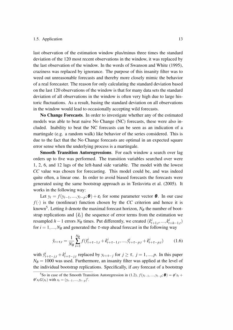
Smooth Transition Autoregressions. For each window a search over lagorders up to five was performed. The transition variables searched over were1, 2, 6, and 12 lags of the left-hand side variable. The model with the lowestCC value was chosen for forecasting. This model could be, and was indeedquite often, a linear one. In order to avoid biased forecasts the forecasts weregenerated using the same bootstrap approach as in Terasvirta et al. (2005). Itworks in the following way:
Let yt = f (yt−1, ...,yt−p;θθθ) + εt for some parameter vector θθθ . In our casef (·) is the (nonlinear) function chosen by the CC criterion and hence it isknown5. Letting h denote the maximal forecast horizon, NB the number of boot-strap replications and εt the sequence of error terms from the estimation weresampled h−1 errors NB times. Put differently, we created (ε i
t+1,t , ..., εit+h−1,t)
for i = 1, ...,NB and generated the τ-step ahead forecast in the following way
yt+τ,t =1
NB
NB
∑i=1
f (yit+τ−1,t + ε
it+τ−1,t , ..., y
it+τ−p,t + ε
it+τ−p,t) (1.6)
with yit+τ− j,t + ε i
t+τ− j,t replaced by yt+τ− j for j ≥ τ, j = 1, ..., p. In this paperNB = 1000 was used. Furthermore, an insanity filter was applied at the level ofthe individual bootstrap replications. Specifically, if any forecast of a bootstrap
5So in case of the Smooth Transition Autoregression in (1.2), f (yt−1, ...,yt−p;θθθ) = φ ′xt +θ ′xtG(st) with xt = (yt−1, ...,yt−p)′.

14 Chapter 1. Forecasting with Universal Approximators and a Learning Algorithm
sample path did not belong to the interval consisting of the last observation of thegiven window plus minus 3 times the standard deviation of the 120 most recentobservations of the window, then the whole bootstrap path was discarded.
Kolmogorov-Gabor polynomials. For each window we searched over mod-els with at most five lags and the highest degree of the polynomial was five. Sincethe number of parameters increases rapidly as a function of the number of lagsand the degree of the polynomial, we implemented a parameter cap of 50 suchthat specifications containing more than 50 parameters were ignored. Amongthe remaining models the one with the lowest CC value was chosen. Due to thenon-affinity of the Kolmogorov-Gabor polynomials, the forecasts were obtainedusing the bootstrap technique outlined above. An insanity filter of the same kindas the one applied to the STR was used.
Artificial Neural Networks. In each window single hidden layer feedfor-ward networks with at most five lags and five hidden units were estimated.Model specification and estimation were carried out using the QuickNet algo-rithm of White (2006)6. The model with the lowest CC value was chosen forforecasting, and as for all non-affine models, the forecasts were generated usinga bootstrap approach combined with the insanity filter outlined for the STR.
Elliptic Basis Function Networks. Models with at most five lags and nomore than five hidden units were estimated in each window. G was chosen as in(1.1). The models considered were of the following form:
yt = αq +β′qxt +
q
∑i=1
wiq exp
− n
∑j=1
(xt, j− ci j)2
2(nσi j)2
(1.7)
where xt = (yt−1, ...,yt−n), n = 1, ...,5. The multiplication of σi j by n was donefor practical reasons. In some initial experiments the hidden units had a verysmall radius of activity – in particular if many explanatory variables were in-cluded. By rescaling the width parameters proportionally to the number of ex-planatory variables this numerical problem was alleviated.
EBF networks can be estimated in many ways. We settled for a procedurewhich learns the centroids and width parameters unsupervised (only the righthand side variables were used to determine the centroids and width parameters
6As discussed in White (2006) the parameter estimates from QuickNet can in principle beused as starting values in a non linear least squares estimation. However, White (2006) alsoshows in a series of experiments that this does not seem to improve the forecast accuracy of theANN. In many cases the estimation simply breaks down in this highly nonlinear problem.

1.5. Application 15
without access to the associated left hand side variables). After having deter-mined these, the problem is linear and the wis can be found by linear regression.This resembles the structure of QuickNet since the problem is split into two parts.First, the centroids and smoothing parameters are found by a grid search. Havingdone this, the problem becomes linear, and one can determine the wis by linearregression.
We now explain how our grid is constructed. Let 1≤ n≤ 5 be given.
1. For 1 ≤ j ≤ n sort yt− j in ascending order and divide it into five clustersof equally many observations, i.e the splits were made at the quintiles7.
2. Within each cluster of yt− j calculate the mean and standard deviations.These are our candidates for ci j and σi j in (1.7). This yields five pairs ofcentroids and width parameters for each yt− j, j = 1, ...,n.
3. Take all possible combinations of centroid-width parameter pairs. Thisyields a grid of cardinality 5n. A typical element of the grid takes the form(ci11, σi11), ...,(cinn, σinn)
, 1≤ i1, ..., in ≤ 5.
We are now in a position to describe the details of our proposed estimationalgorithm which one could call the QuickEBF due to its similarity to the Quick-Net. Choose n ∈ 1, ...,5 and let xt = (yt−1, ...,yt−n) be given, i.e., consider afixed vector of explanatory variables.
1. Determine α0 and β0 by regressing yt on a constant and xt . Also calculatethe value of the choice criterion CC.
2. Each of the 5n grid points corresponds to a hidden unit (elliptic basis func-tion). For q = 1, ...,5, add hidden units one by one in the following way:Determine αq, βq, and wi,q, i = 1, ...,q by OLS for each potential hiddenunit not previously chosen, i.e., for each point in the grid of c’s and σ ’s.Notice that the weights of previously added hidden units as well as αq andβq are allowed to change as further hidden units are added, whereas thecentroids and smoothing parameters remain fixed once they have been de-termined. This resembles the QuickNet algorithm of White (2006). Calcu-late the value of the choice criterion and add the hidden unit which yieldsthe lowest value of CC.
7One could also split each explanatory variable into more than five clusters and therebyobtain an even finer grid. Here five clusters were chosen for each series since the maximumnumber of hidden units was five.

16 Chapter 1. Forecasting with Universal Approximators and a Learning Algorithm
3. Repeat (1) and (2) for all choices of explanatory variables which in ourcase corresponds to xt = (yt−1, ...,yt−n), n = 1, ...,5. Choose n∈ 1, ...,5and q∈ 0, ...,5 such that they minimize the choice criterion and forecastwith the parameter estimates corresponding to these values.
The forecasts of the Elliptic Basis Function Network were produced by the samebootstrap procedure as that for the aforementioned nonlinear models. Unreason-able forecasts were weeded out by the same insanity filter as outlined for theSTR.
One notices that the QuickEBF is easy to implement since after having fixedthe centroids and width parameters it consists of linear regressions. This is con-venient since at the outset the EBF is not easy to estimate because the centroidsand width parameters are not identified when more than one hidden unit is in-cluded. The QuickEBF deals with this in an easy way.
Forecast Combinations. As mentioned in the Introduction, a major aim ofthe work is considering the effects of combining forecasts on forecast accuracy.Two equal weighting schemes were employed: (i) Equal weighting of all modelsand (ii) equal weighting of the three universal approximators.
As mentioned in Section 1.4, one must assume the existence of an interval[a,b] such that (xt+τ,t ,yt+τ) ∈ [a,b]n+1 in order to give explicit loss bounds forthe WAA. Our solution to this problem was the following. Let Y denote thelast observation in the first estimation window and s the standard deviation ofthe 120 most recent observations of the first estimation window. Then we chose[a,b] = [Y − 3s,Y + 3s] which in the vast majority of the cases was more thanwide enough to contain all forecasts and realizations8. The corresponding valueof c was denoted cB. The reason for only calculating s on the basis of the last 120observations was the same as that given in the treatment of the insanity filter.
The results for the WAA with c = cB were called WAA(cB). In order toinvestigate the performance of the WAA for smaller values of c, i.e., a fasteradjustment of the weights towards the models that have performed well in themore recent past, we calculated the forecasts of the WAA with c = cL = cB
100 .These forecasts were called WAA(cL). Both WAA based forecasts were appliedseparately to each horizon. This allowed the WAA to attach different weights toeach model for different horizons. This is sensible since models performing wellat short horizons need not perform well in long term forecasting, and vice versa.
8This fits well with the choice of insanity filter since it is exactly observations outside [Y −3s,Y +3s] we regard as insane.

1.5. Application 17
All combination schemes in this paper were applied separately to each horizon.To compare the WAA to another loss based algorithm we performed fore-
casting using inverse MSE weights with the MSE calculated from all previousforecast errors. Since the loss of a τ periods ahead forecast will not be observeduntil these τ periods have elapsed, one would have to initialize the weights ofthe loss based algorithms (WAA and MSE) in some fashion. We did this bynot beginning the comparison until the first losses at the relevant horizon wererealized. Consequently, for τ periods ahead forecasts the actual number of eval-uation periods was 72-τ .
Results
Tables 1.3-1.8 in the Appendix report the Root Mean Square Forecast Errors(RMSFE) of each point forecast relative to the RMSFE of the linear autoregres-sive specification. The numbers in brackets are the RMSFE of the linear autore-gressive specification. Empty sections in the tables refer to series for which datawas unavailable.
Inspection of these tables reveals that no single model systematically outper-forms the others. This is in line with Terasvirta et al. (2005). One notices thatfor some time series there are models which have a relative RMSFE of 1 at allhorizons. This indicates that the linear specification was chosen in each windowfor this model class. Table 1.1 summarizes Tables 1.3-1.8. It shows the RMSFEratios as well as the rank of each model across all data sets and all horizons(Overall), all horizons (Horizon), and all types of data sets (Data).
Performance of the Universal Approximators
An aim of the paper was to consider the performance of universal approxima-tors. Table 1.1 reveals that the Elliptic Basis Function Networks outperformthe Kolmogorov-Gabor polynomials and the Artificial Neural Networks overall.We will explain this result below. All universal approximators perform well forthe inflation series with relative RMSFE clearly below 1. In fact, for Denmark,France, and Italy all universal approximators yield more accurate forecasts at allhorizons than the linear AR for this series. This is also the case for the forecastsof French industrial production. On the other hand there does not exist a sin-gle country/variable combination for which all the universal approximators haverelative RMSFE above 1 at all horizons.

18 Chapter 1. Forecasting with Universal Approximators and a Learning Algorithm
Hor
izon
Dat
a
Ove
rall
13
612
24IN
FIP
IM
U
AR
1.00
0(11
)1.
000(
7)1.
000(
8)1.
000(
12)
1.00
0(8)
1.00
0(12
)1.
000(
12)
1.00
0(8)
1.00
0(9)
1.00
0(1)
1.00
0(7)
NC
0.98
0(6)
0.99
9(5)
0.98
9(7)
0.97
7(6)
1.00
8(11
)0.
926(
7)0.
852(
1)1.
118(
12)
0.86
8(1)
1.15
4(12
)0.
990(
6)ST
R0.
990(
8)1.
015(
9)1.
006(
9)0.
992(
9)1.
014(
12)
0.92
3(5)
0.88
2(9)
1.06
4(11
)0.
962(
7)1.
048(
8)1.
028(
11)
KG
1.00
5(12
)1.
058(
12)
1.00
9(10
)0.
991(
8)0.
994(
7)0.
972(
11)
0.87
3(7)
1.00
8(9)
1.07
5(11
)1.
082(
10)
1.03
0(12
)A
NN
0.99
8(10
)1.
026(
11)
1.01
1(11
)0.
998(
11)
1.00
3(9)
0.95
1(9)
0.87
7(8)
0.99
5(7)
1.08
0(12
)1.
049(
9)1.
020(
10)
EB
F0.
980(
7)0.
999(
6)0.
988(
6)0.
981(
7)0.
979(
6)0.
954(
10)
0.92
7(11
)0.
981(
5)0.
991(
8)1.
017(
2)1.
004(
8)E
Q(A
ll)0.
948(
3)0.
984(
3)0.
965(
2)0.
950(
3)0.
950(
4)0.
893(
3)0.
860(
3)0.
972(
3)0.
955(
6)1.
027(
4)0.
968(
1)E
Q(U
A)
0.96
6(5)
1.00
1(8)
0.97
7(5)
0.96
5(5)
0.96
5(5)
0.92
3(6)
0.86
4(5)
0.97
8(4)
1.01
1(10
)1.
028(
6)0.
986(
5)W
AA
(cB)
0.94
8(2)
0.98
4(2)
0.96
5(3)
0.94
9(2)
0.94
6(2)
0.89
4(4)
0.86
3(4)
0.96
9(2)
0.95
1(5)
1.02
7(5)
0.96
8(2)
WA
A(c
L)
0.95
0(4)
0.98
8(4)
0.97
1(4)
0.95
4(4)
0.94
8(3)
0.88
9(2)
0.86
9(6)
0.99
2(6)
0.91
3(2)
1.03
9(7)
0.98
0(4)
MSE
0.93
9(1)
0.98
3(1)
0.96
4(1)
0.94
2(1)
0.93
4(1)
0.87
2(1)
0.85
7(2)
0.96
5(1)
0.92
2(3)
1.02
6(3)
0.96
9(3)
Las
t0.
993(
9)1.
021(
10)
1.01
6(12
)0.
995(
10)
1.00
6(10
)0.
927(
8)0.
909(
10)
1.05
7(10
)0.
949(
4)1.
086(
11)
1.00
9(9)
Tabl
e1.
1:R
elat
ive
RM
SFE
ratio
san
dth
eco
rres
pond
ing
rank
s(i
nas
cend
ing
orde
r)fo
rth
eov
eral
l,th
eho
rizo
nwis
e,an
dda
taw
ise
perf
orm
ance
ofea
chfo
reca
stpr
oced
ure.
The
ratio
sw
ere
calc
ulat
edby
taki
ngth
eav
erag
eov
erth
ere
leva
ntra
tios
from
Tabl
es1.
3th
roug
h1.
8.Fo
rexa
mpl
e,th
eho
rizo
nwis
epe
rfor
man
cew
asca
lcul
ated
byta
king
the
aver
age
ofal
lrat
ios
ata
fixed
fore
cast
hori
zon
acro
ssal
ldat
ase
ts.
AR
:L
inea
rA
utor
egre
ssio
n,N
C:
No
Cha
nge
fore
cast
s,ST
R:
Smoo
thTr
ansi
tion
Reg
ress
ion,
KG
:K
olm
ogor
ov-G
abor
poly
nom
ial,
AN
N:
Art
ifici
alN
eura
lN
etw
ork,
EB
F:E
llipt
icB
asis
Func
tion
netw
ork,
EQ
(All)
:E
qual
wei
ghtin
gof
all
indi
vidu
alm
odel
s,E
Q(U
A):
Equ
alw
eigh
ting
ofth
eun
iver
sala
ppro
xim
ator
s,W
AA
(cB
):W
AA
with
c=
c B,W
AA
(cL):
WA
Aw
ithc
=c L
,MSE
:Wei
ghtin
gby
inve
rse
MSE
,Las
t:Fo
reca
stin
gw
ithth
em
odel
whi
chha
sth
ebe
stpr
evio
usly
real
ized
fore
cast
atth
egi
ven
hori
zon.

1.5. Application 19
Furthermore, Table 1.1 shows that the performance of the universal approxi-mators in general improves as the forecast horizon gets longer. For the EBF thisrelationship is even monotonic. This pattern can be found for all three universalapproximators at the same time for, for example, the Japanese unemploymentseries and for the KG and EBF for Danish interest rates. The performance of theKG for the Danish interest rate series also illustrates that the relative RMSFEneed not be decreasing when monotonic. In particular, the performance of theKG worsens as the forecast horizon gets longer. The fact that the most extremeforecasts (good as well as bad) are found at the longest forecast horizon is nosurprise given that the forecasts are carried out recursively. This is due to thefact that the benefit/loss from a superior/inferior specification is accumulated asthe forecasts are iterated forward.
Overall, the EBF is the best performing universal approximator. In fact, Ta-ble 1.1 reveals that the linear autoregression is beaten at all forecast horizonsby the EBF. The EBF also outperforms the other universal approximators at allhorizons except the 24 month horizon where it is outperformed by the ANN. Thereason for the promising performance of the EBF is that it takes the best fromtwo extremes. For 21 of the 47 data sets the EBF is actually just the linear AR(no hidden units are chosen)9. When this purely linear specification is chosen,it is often the case that the two other universal approximators perform less wellcompared to the linear AR, see for example the money supply series for Den-mark, Germany, and Sweden. When basing the overall performance of the EBFonly on those data sets in which the EBF differs from the linear AR, we get anoverall relative RMSFE of .96. So for 21 data sets the EBF equals the linear AR,and for those data sets for which the two models differ, the EBF on average does4% better.
Table 1.2 contains the lowest and highest relative RMSFE of each proce-dure across all datasets. The table also shows the number of times the relativeRMSFE of each procedure was below .9 as well as how often it was above 1.1.It is of interest that out of 47×5 = 235 relative RMSFE (number of table entriesfor each procedure in Tables 1.3-1.8) the EBF never has a relative RMSFE ex-ceeding 1.189. This value is much lower than the corresponding value for anyof the other universal approximators. The Kolmogorov-Gabor polynomials, forexample, have a worst case relative RMSFE of 1.91. Actually the worst case per-formance of the EBF is better than the worst case performance of any forecasting
9For the Swedish unemployment series the EBF has a relative RMSFE of 1 due to roundingerror - not due to the fact that a linear model was chosen every time.

20 Chapter 1. Forecasting with Universal Approximators and a Learning Algorithm
method considered - including forecast combinations. Furthermore, it only hap-pens five times that the EBF performs more than 10% worse than the linear AR.This too is better than any other forecasting procedure and much lower than anynon-combinatorial method. Hence, it is reasonable to conclude that the risk ofvery bad forecasts with the EBF is limited. This fact is emphasized by the abovefinding that the forecasts of the EBF often simply equal the forecasts of the lin-ear AR in cases where the latter performs well. So it is not surprising that theEBF has relatively few extreme forecasts.
It is also worth noticing that the lowest relative RMSFE obtained by the EBFis lower than the corresponding number for the two other universal approxi-mators. But then, the EBF has fewer relative RMSFEs below 0.9 than any othermethod. Nevertheless, our conclusion is that the EBF is a stable procedure whichcombines the best from linear and nonlinear forecasting procedures.
NC STR KG ANN EBF EQ(All) EQ(UA) WAA(cB) WAA(cL) MSE Last
Lowest 0.286 0.297 0.497 0.421 0.411 0.459 0.435 0.437 0.301 0.319 0.356Highest 1.782 1.555 1.911 1.701 1.189 1.249 1.393 1.241 1.417 1.274 1.557# < 0.9 67 43 47 33 21 49 37 49 54 52 49# > 1.1 48 46 43 27 5 11 11 9 13 6 41
Table 1.2: The table contains the lowest as well as the highest relative RMSFE of each procedure(except AR) and the number of relative RMSFE below 0.9 and above 1.1 (except AR) calculated fromTables 1.3 through 1.8. NC: No Change forecasts, STR: Smooth Transition Regression, KG: Kolmogorov-Gabor polynomial, ANN: Artificial Neural Network, EBF: Elliptic Basis Function network, EQ(All): Equalweighting of all individual models, EQ(UA): Equal weighting of the universal approximators, WAA(cB):WAA with c = cB, WAA(cL): WAA with c = cL, MSE: Weighting by inverse MSE, Last: Forecasting withthe model which has the best previously realized forecast at the given horizon.
Smooth Transition and No Change forecasts
Table 1.1 reveals that the Smooth Transition model performs very well at the 24month horizon. For the Italian industrial production series it obtains a relativeRMSFE as low as 0.297 at this horizon. On the other hand Table 1.2 shows thatthe STR is the only procedure which has more relative RMSFE above 1.1 thanbelow 0.9. In particular it has 46 values above 1.1 which indicates that it is a lessstable procedure than the EBF. As opposed to Stock and Watson (1999) we findthat the STR can match the ANN. We also find that the ANN in general has itslowest RMSFE at the longest forecast horizon. This too is in opposition to Stockand Watson (1999). It should be mentioned, however, that Stock and Watson(1999) carry out their forecasts directly while we do it recursively. Hence, the

1.5. Application 21
results are not directly comparable. Finally, we notice that the STR performswell for the interest rate series except for Denmark, Japan, and Norway.
It is well known that the No Change forecasts are optimal in an expectedsquare error sense if the series of interest is a martingale. Table 1.1 indicates thatthe No Change forecasts perform well for the inflation and interest rate series. Infact they perform better than any other procedure for these series. However, theopposite is the case for the industrial production and money supply series wherethey perform worse than any other method. This lack of stability is confirmedby Table 1.2 which shows that the No Change forecasts are the procedure withmost relative RMSFE below 0.9 and above 1.1. In order to interpret these resultswe test whether each of the series is a random walk against a stationary AR(1)with intercept. Only for 1 out of 11 inflation series this hypothesis is rejectedat a 5% significance level. For the interest rate series this hypothesis is neverrejected. Consequently, the No Change forecasts should perform well for thesedata sets. For the industrial production series the random walk is rejected 5 outof 10 times while the corresponding numbers for the money supply series are1 out of 6. These results are more mixed. While it is sensible that the randomwalk hypothesis is rejected rather often for the industrial production series, it isrejected less often than expected for the money supply series.
Importance of the Insanity Filter
Applying an insanity filter turned out to be very important. Forecasting recur-sively 24 months ahead meant that some of the bootstrap paths yielded clearlyunrealistic forecasts. This was particularly pronounced for the Kolmogorov-Gabor polynomials which are of an explosive nature due to their polynomialstructure. A single insane forecast can (and turned out to) make even the av-erage over bootstrap paths a bad forecast, and so it is vital to remove insanepaths. The problem was less pronounced for the other nonlinear models forwhich the hidden units are bounded. Still an insanity filter was important forthese too - while explosive less often, they could yield very unreasonable fore-casts. The number of bootstrap paths removed by the insanity filter could varygreatly. Sometimes very few (none) were removed, while in other cases severalhundred were weeded out by the insanity filter.

22 Chapter 1. Forecasting with Universal Approximators and a Learning Algorithm
Forecast Combinations
A general conclusion is that it pays of to combine forecasts. The forecast com-bination schemes in general outperform the individual methods. This is in linewith Stock and Watson (1999) and Terasvirta et al. (2005). Weighting by inverseMSE performs best overall and is also superior at each forecast horizon as seenfrom Table 1.1. The Weighted Average Algorithm performs roughly the same forboth values of c. Table 1.2 reveals that c = cL gives more extreme values (goodas well as bad) than c = cB. In total these two effects balance each other andWAA(cB) and WAA(cL) perform equally well. The inverse MSE scheme per-forms slightly better than the two versions of the WAA since it has as many goodoutcomes (< 0.9) as WAA(cL) and as few bad outcomes (> 1.1) as WAA(cB),see Table 1.2.
Regarding equal weighting schemes, combinig all models is preferable toonly combining the universal approximators. This is the case overall, at all hori-zons, and for all types of data sets. Table 1.2 indicates that the reason for this dif-ference is more low (< 0.9) relative RMSFEs while the number of high (> 1.1)relative RMSFEs is roughly unaltered compared to only combining the universalapproximators.
Finally, Figure 1.1 in the Appendix shows the development of the weights inthe WAA for c = cL for the industrial production series for the UK at all horizons.This series was chosen since it illustrates some interesting features of the WAA.When inspecting Table 1.7 it is not surprising that as the forecast horizon in-creases more weight is given to the Kolmogorov-Gabor polynomials since thesedid well at the long horizons for this series. By the same token it is sensible thatthe linear autoregression receives less weight as the forecast horizon becomeslonger. When inspecting the development of the weights at the 24-month hori-zon in Figure 1.1, it is interesting to see how the weights of the WAA can adaptover time as the relative performance of the individual models changes. In par-ticular, the relative weights assigned to the Elliptic Basis Function Networks andthe Kolmogorov-Gabor polynomials change around period 35.
1.6 Conclusions
In this paper we consider the forecasting performance of nonlinear models rela-tive to linear autoregressions. Three of the model classes employed are universalapproximators - the Kolmogorov-Gabor polynomials, the Artificial Neural Net-

1.6. Conclusions 23
works, and the Elliptic Basis Function Networks.Regarding the first question posed in the introduction, we find that there are
potential gains to be made from using universal approximators. In particular,the Elliptic Basis Functions turn out to deliver good forecasts. Their main meritis that they combine the best from two worlds. In the cases where the linearautoregressions tend to be superior, the EBF equals these and in the cases wherethere seem to be gains to be made from using hidden units, these are includedinto the EBF. As opposed to many other nonlinear procedures, forecasting withan EBF is not too risky either since even the worst performance observed isnot too bad. Furthermore, the proposed estimation strategy is not difficult toimplement since it essentially amounts to running a series of linear regressions.Hence, we believe that the EBF is a useful addition to the set of macroeconomicforecasters.
Secondly, when forecasting recursively with nonlinear models an insanityfilter is definitely advisable since even a single wild bootstrap path can affect theforecast adversely.
The No Change forecasts also perform quite well but their performance isvery unstable compared to the one of the EBF.
Thirdly, we find that the WAA is unable to outperform more standard meth-ods. From a practitioners point of view it is encouraging that simple equalweighting does so well since it is easy to understand and implement.
All forecasts are carried out recursively in this paper. Hence a possible exten-sion which we are currently working on is to investigate whether there are gainsto be made by forecasting directly with the universal approximators. Other waysof selecting the hidden units could also be studied. Finally, we consider uni-variate procedures in this paper. Further gains in the forecast accuracy might beachievable by applying the universal approximators - in particular the EBF - ina multivariate setting.

24 Chapter 1. Forecasting with Universal Approximators and a Learning Algorithm
1.7 Appendix
0 5 10 15 20 25 30 35 40 45 50 55 60 65 70
0.25
0.50
Forecast horizon: 1 months, WAA(cL)AR STR ANN
NC KG EBF
0 5 10 15 20 25 30 35 40 45 50 55 60 65 70
0.5
1.0 Forecast horizon: 3 months, WAA(cL)AR STR ANN
NC KG EBF
0 5 10 15 20 25 30 35 40 45 50 55 60 65
0.5
1.0 Forecast horizon: 6 months, WAA(cL)AR STR ANN
NC KG EBF
0 5 10 15 20 25 30 35 40 45 50 55 60
0.5
1.0 Forecast horizon: 12 months, WAA(cL)AR STR ANN
NC KG EBF
0 5 10 15 20 25 30 35 40 45 50
0.5
1.0 Forecast horizon: 24 months, WAA(cL)AR STR ANN
NC KG EBF
Figure 1.1: Development of the weights of the WAA applied to the Industrial Production seriesfor the UK with c = cL.

Infla
tion
Indu
stri
alPr
oduc
tion
Inte
rest
Rat
eM
oney
Supp
lyU
nem
ploy
men
t
Can
ada
13
612
241
36
1224
13
612
241
36
1224
13
612
24
AR
[0.5
38]
[0.9
40]
[1.2
95]
[1.6
44]
[1.2
84]
[0.5
19]
[0.7
69]
[1.1
65]
[1.2
53]
[1.3
77]
[0.1
72]
[0.2
74]
[0.3
99]
[0.6
72]
[1.1
44]
[0.9
23]
[1.6
74]
[2.2
63]
[2.5
10]
[1.8
23]
[0.1
49]
[0.2
48]
[0.3
63]
[0.4
75]
[0.8
13]
NC
0.97
20.
983
0.97
70.
966
0.79
41.
085
1.08
91.
062
1.13
50.
826
0.94
90.
896
0.80
40.
666
0.58
31.
033
1.08
61.
204
1.58
01.
186
0.99
30.
973
0.96
60.
922
0.94
2ST
R0.
999
0.99
00.
998
0.99
10.
901
0.99
20.
968
0.97
01.
017
0.73
00.
982
0.94
00.
867
0.74
50.
691
0.99
61.
007
1.03
01.
198
0.92
31.
016
1.03
31.
053
1.11
61.
132
KG
0.98
50.
962
0.94
00.
885
0.65
91.
044
1.18
01.
271
1.30
80.
988
1.01
01.
025
1.07
01.
112
1.07
81.
027
1.03
11.
106
1.37
01.
074
1.03
01.
059
1.07
91.
080
1.07
9A
NN
1.01
31.
000
0.99
30.
966
0.84
31.
021
1.11
11.
125
1.11
60.
881
0.99
31.
000
0.99
50.
921
0.81
61.
021
1.01
01.
034
1.18
91.
020
1.00
01.
000
1.00
01.
000
1.00
0E
BF
1.00
01.
000
1.00
01.
000
1.00
01.
000
1.00
01.
000
1.00
01.
000
1.00
01.
000
1.00
01.
000
1.00
01.
038
1.06
71.
075
1.18
90.
931
1.00
01.
000
1.00
01.
000
1.00
0E
Q(A
ll)0.
992
0.98
50.
980
0.96
10.
838
1.00
51.
029
1.03
21.
010
0.82
60.
981
0.96
40.
939
0.89
60.
849
1.00
61.
019
1.06
21.
249
0.97
91.
001
1.00
11.
007
1.01
01.
022
EQ
(UA
)0.
996
0.98
30.
973
0.94
40.
814
1.01
11.
079
1.10
61.
084
0.91
10.
992
0.99
91.
013
1.00
40.
951
1.01
41.
024
1.06
41.
246
1.00
11.
006
1.01
51.
022
1.02
01.
022
WA
A(c
B)
0.99
20.
985
0.98
00.
960
0.83
41.
005
1.02
91.
031
1.00
50.
825
0.98
10.
964
0.93
90.
894
0.84
21.
006
1.01
91.
062
1.24
10.
977
1.00
11.
001
1.00
71.
010
1.02
3W
AA
(cL)
0.99
00.
985
0.97
40.
910
0.74
61.
005
1.01
61.
002
0.91
40.
718
0.98
10.
960
0.89
90.
763
0.62
91.
008
1.02
01.
078
1.29
71.
002
1.00
11.
001
1.00
61.
006
1.04
6M
SE0.
991
0.98
60.
982
0.96
00.
819
1.00
11.
004
1.01
30.
980
0.78
60.
980
0.96
10.
921
0.81
60.
723
1.00
61.
021
1.07
51.
274
0.96
51.
001
1.00
11.
006
1.01
01.
030
Las
t0.
975
1.00
00.
985
0.97
70.
930
1.06
01.
063
1.01
91.
158
0.88
20.
977
0.95
00.
916
0.73
00.
588
1.02
21.
079
1.11
91.
371
1.01
81.
002
1.00
11.
037
1.04
61.
072
Infla
tion
Indu
stri
alPr
oduc
tion
Inte
rest
Rat
eM
oney
Supp
lyU
nem
ploy
men
t
Den
mar
k1
36
1224
13
612
241
36
1224
13
612
241
36
1224
AR
[0.2
56]
[0.4
16]
[0.6
34]
[1.0
48]
[1.4
72]
[0.1
97]
[0.3
94]
[0.5
73]
[0.9
20]
[1.2
72]
[1.3
07]
[2.7
05]
[3.6
55]
[5.3
03]
[6.3
79]
[0.0
98]
[0.1
97]
[0.3
59]
[0.7
74]
[1.9
44]
NC
0.93
70.
857
0.78
20.
715
0.60
90.
834
0.85
00.
824
0.73
10.
628
1.12
11.
104
1.21
01.
372
1.46
91.
059
1.10
91.
117
1.04
20.
861
STR
1.00
00.
902
0.75
20.
706
0.62
91.
121
1.05
01.
036
1.02
71.
016
0.99
30.
991
1.04
81.
121
1.08
61.
016
1.05
51.
107
1.10
11.
106
KG
0.99
30.
826
0.75
20.
632
0.53
41.
006
1.07
61.
434
1.72
71.
911
0.96
40.
914
0.95
81.
218
1.20
21.
024
1.04
21.
020
1.02
00.
938
AN
N0.
920
0.85
80.
734
0.67
50.
610
1.02
21.
317
1.64
61.
701
1.62
91.
015
1.04
51.
054
1.15
51.
149
1.00
41.
016
1.00
31.
001
0.97
8E
BF
0.97
70.
905
0.84
70.
771
0.68
10.
929
0.90
00.
881
0.80
50.
723
1.00
01.
000
1.00
01.
000
1.00
01.
000
1.00
01.
000
1.00
01.
000
EQ
(All)
0.95
20.
864
0.77
40.
707
0.64
00.
900
0.96
91.
061
1.11
81.
111
0.97
50.
974
1.00
61.
118
1.12
50.
996
1.00
41.
008
1.00
30.
969
EQ
(UA
)0.
942
0.84
10.
750
0.66
90.
596
0.87
61.
011
1.22
51.
359
1.39
30.
967
0.96
90.
983
1.10
81.
100
1.00
01.
009
0.99
70.
999
0.96
9W
AA
(cB)
0.95
20.
863
0.77
00.
697
0.62
20.
900
0.96
91.
051
1.07
01.
002
0.97
50.
974
1.00
51.
111
1.11
60.
996
1.00
41.
008
1.00
30.
969
WA
A(c
L)
0.94
20.
843
0.78
50.
698
0.60
50.
893
0.93
10.
868
0.76
30.
669
0.98
10.
969
1.01
31.
016
1.04
60.
996
1.00
61.
016
1.04
20.
965
MSE
0.94
70.
857
0.75
90.
679
0.59
90.
886
0.93
20.
933
0.85
30.
749
0.97
50.
982
1.01
21.
107
1.09
10.
997
1.00
71.
019
1.03
20.
980
Las
t0.
956
0.88
90.
828
0.82
90.
601
0.95
21.
076
0.91
80.
806
0.66
01.
096
1.02
11.
027
1.27
41.
168
0.99
41.
011
1.02
01.
041
1.02
3
Tabl
e1.
3:R
elat
ive
Roo
tMea
nSq
uare
Fore
cast
Err
orra
tioso
feac
hm
odel
with
the
linea
raut
oreg
ress
ion
bein
gth
ebe
nchm
ark.
The
first
row
inea
chpa
nelc
onta
ins
the
Roo
tMea
nSq
uare
Fore
cast
Err
orof
the
linea
rau
tore
gres
sion
inpa
rent
hese
s.A
R:L
inea
rA
utor
egre
ssio
n,N
C:N
oC
hang
efo
reca
sts,
STR
:Sm
ooth
Tran
sitio
nR
egre
ssio
n,K
G:K
olm
ogor
ov-G
abor
poly
nom
ial,
AN
N:A
rtifi
cial
Neu
ralN
etw
ork,
EB
F:E
llipt
icB
asis
Func
tion
netw
ork,
EQ
(All)
:Equ
alw
eigh
ting
ofal
lind
ivid
ual
mod
els,
EQ
(UA
):E
qual
wei
ghtin
gof
the
univ
ersa
lapp
roxi
mat
ors,
WA
A(c
B):
WA
Aw
ithc
=c B
,WA
A(c
L):
WA
Aw
ithc
=c L
,MSE
:Wei
ghtin
gby
inve
rse
MSE
,L
ast:
Fore
cast
ing
with
the
mod
elw
hich
has
the
best
prev
ious
lyre
aliz
edfo
reca
stat
the
give
nho
rizo
n.

Infla
tion
Indu
stri
alPr
oduc
tion
Inte
rest
Rat
eM
oney
Supp
lyU
nem
ploy
men
t
Finl
and
13
612
241
36
1224
13
612
241
36
1224
13
612
24
AR
[0.3
20]
[0.5
44]
[0.7
94]
[1.2
77]
[1.3
29]
[3.4
89]
[4.7
51]
[5.1
54]
[5.1
76]
[6.0
58]
[0.1
00]
[0.2
24]
[0.3
44]
[0.4
46]
[0.9
45]
NC
0.94
50.
869
0.79
20.
748
1.32
40.
964
1.03
21.
262
1.53
51.
278
0.89
40.
911
0.94
01.
272
1.30
9ST
R0.
998
0.91
90.
799
0.73
31.
114
0.98
70.
986
1.08
11.
152
0.97
80.
826
0.98
41.
033
1.10
21.
381
KG
1.01
40.
946
0.81
50.
734
1.09
51.
001
0.99
11.
015
1.04
51.
115
0.90
10.
900
0.86
50.
899
0.84
6A
NN
1.00
01.
022
1.01
61.
036
1.30
00.
956
0.96
61.
026
1.09
51.
015
1.00
41.
064
1.18
71.
444
1.49
4E
BF
1.00
01.
000
1.00
01.
000
1.00
00.
950
0.93
90.
976
1.02
71.
002
1.00
01.
000
1.00
01.
000
1.00
0E
Q(A
ll)0.
982
0.94
30.
865
0.79
40.
924
0.93
90.
953
1.03
11.
122
1.03
30.
885
0.93
10.
945
1.01
81.
118
EQ
(UA
)0.
997
0.98
00.
917
0.86
40.
965
0.95
50.
957
0.99
81.
047
1.03
70.
957
0.97
30.
988
1.04
11.
063
WA
A(c
B)
0.98
20.
942
0.86
10.
795
1.16
10.
939
0.95
41.
029
1.10
21.
033
0.88
50.
931
0.94
41.
018
1.11
7W
AA
(cL)
0.97
90.
914
0.80
20.
751
1.32
80.
968
0.99
91.
063
1.04
21.
003
0.88
50.
930
0.93
71.
003
1.06
7M
SE0.
984
0.93
50.
833
0.75
31.
038
0.93
80.
956
1.03
01.
088
1.03
20.
876
0.92
10.
901
0.98
81.
102
Las
t1.
015
0.94
40.
887
0.70
71.
138
0.94
81.
024
1.20
81.
096
1.18
50.
880
1.02
90.
887
0.92
81.
067
Infla
tion
Indu
stri
alPr
oduc
tion
Inte
rest
Rat
eM
oney
Supp
lyU
nem
ploy
men
t
Fran
ce1
36
1224
13
612
241
36
1224
13
612
241
36
1224
AR
[0.3
19]
[0.5
34]
[0.6
21]
[0.7
74]
[1.1
03]
[1.4
26]
[1.8
11]
[2.2
46]
[2.3
96]
[2.0
08]
[0.1
54]
[0.3
27]
[0.4
85]
[0.7
64]
[0.9
76]
[0.0
61]
[0.1
14]
[0.2
22]
[0.4
80]
[1.0
18]
NC
0.93
90.
821
0.70
70.
632
0.59
11.
044
1.01
10.
971
1.04
11.
187
0.99
20.
935
0.87
60.
797
0.73
31.
061
1.19
41.
163
1.06
30.
927
STR
0.93
00.
810
0.69
30.
663
0.65
41.
010
0.98
70.
986
0.95
90.
887
0.99
30.
994
0.98
60.
965
0.93
71.
034
1.03
51.
009
0.92
40.
901
KG
0.99
70.
821
0.68
90.
622
0.61
00.
998
0.93
30.
819
0.79
50.
806
0.98
90.
957
0.96
80.
958
0.97
91.
497
1.25
11.
176
1.22
31.
377
AN
N0.
916
0.79
80.
705
0.63
70.
591
0.95
90.
880
0.77
80.
756
0.79
11.
000
1.00
01.
000
1.00
01.
000
1.00
31.
004
1.00
61.
003
1.00
1E
BF
0.92
60.
805
0.69
40.
697
0.63
90.
972
0.94
90.
877
0.89
60.
924
1.00
01.
000
1.00
01.
000
1.00
01.
000
1.00
01.
000
1.00
01.
000
EQ
(All)
0.93
60.
825
0.72
60.
685
0.65
60.
967
0.90
70.
840
0.81
60.
809
0.99
10.
975
0.96
50.
945
0.92
11.
014
1.00
81.
007
1.00
01.
018
EQ
(UA
)0.
930
0.79
70.
683
0.64
30.
610
0.95
80.
901
0.80
50.
794
0.81
10.
993
0.98
00.
984
0.98
10.
982
1.06
31.
033
1.03
61.
057
1.11
3W
AA
(cB)
0.93
60.
824
0.72
20.
678
0.64
60.
967
0.90
70.
840
0.81
50.
805
0.99
10.
975
0.96
40.
944
0.91
91.
014
1.00
81.
007
1.00
01.
018
WA
A(c
L)
0.93
20.
813
0.68
90.
659
0.61
80.
974
0.92
00.
841
0.78
90.
759
0.99
10.
973
0.94
70.
876
0.77
91.
012
1.00
81.
018
1.01
61.
036
MSE
0.93
60.
826
0.70
80.
683
0.64
50.
968
0.91
60.
844
0.81
60.
791
0.99
10.
972
0.95
50.
917
0.85
41.
011
1.00
71.
012
1.00
81.
040
Las
t0.
953
0.89
30.
778
0.79
50.
729
1.02
10.
985
0.84
60.
958
0.94
60.
982
0.98
40.
938
0.87
30.
733
1.10
61.
123
1.13
41.
105
1.04
1
Tabl
e1.
4:R
elat
ive
Roo
tMea
nSq
uare
Fore
cast
Err
orra
tioso
feac
hm
odel
with
the
linea
raut
oreg
ress
ion
bein
gth
ebe
nchm
ark.
The
first
row
inea
chpa
nelc
onta
ins
the
Roo
tMea
nSq
uare
Fore
cast
Err
orof
the
linea
rau
tore
gres
sion
inpa
rent
hese
s.A
R:L
inea
rA
utor
egre
ssio
n,N
C:N
oC
hang
efo
reca
sts,
STR
:Sm
ooth
Tran
sitio
nR
egre
ssio
n,K
G:K
olm
ogor
ov-G
abor
poly
nom
ial,
AN
N:A
rtifi
cial
Neu
ralN
etw
ork,
EB
F:E
llipt
icB
asis
Func
tion
netw
ork,
EQ
(All)
:Equ
alw
eigh
ting
ofal
lind
ivid
ual
mod
els,
EQ
(UA
):E
qual
wei
ghtin
gof
the
univ
ersa
lapp
roxi
mat
ors,
WA
A(c
B):
WA
Aw
ithc
=c B
,WA
A(c
L):
WA
Aw
ithc
=c L
,MSE
:Wei
ghtin
gby
inve
rse
MSE
,L
ast:
Fore
cast
ing
with
the
mod
elw
hich
has
the
best
prev
ious
lyre
aliz
edfo
reca
stat
the
give
nho
rizo
n.

Infla
tion
Indu
stri
alPr
oduc
tion
Inte
rest
Rat
eM
oney
Supp
lyU
nem
ploy
men
t
Ger
man
y1
36
1224
13
612
241
36
1224
13
612
241
36
1224
AR
[0.3
16]
[0.4
26]
[0.5
36]
[0.7
14]
[0.5
34]
[1.4
64]
[1.9
76]
[2.8
37]
[2.5
12]
[2.8
36]
[0.1
55]
[0.3
42]
[0.5
43]
[0.9
13]
[1.2
92]
[2.2
55]
[3.3
23]
[2.5
44]
[3.1
60]
[3.1
41]
[0.1
22]
[0.3
01]
[0.5
21]
[0.9
67]
[1.8
96]
NC
0.97
60.
980
0.95
00.
912
1.40
61.
086
1.06
91.
126
1.31
21.
241
0.98
80.
892
0.78
50.
664
0.53
91.
039
1.11
91.
331
1.53
91.
499
1.02
51.
017
0.99
20.
987
0.96
5ST
R1.
011
1.02
11.
015
0.98
71.
187
1.01
51.
043
1.05
51.
379
1.11
80.
982
0.93
60.
861
0.75
50.
638
1.03
51.
100
1.11
31.
141
1.00
10.
943
0.99
71.
015
1.02
20.
982
KG
1.06
81.
046
1.04
41.
010
1.16
81.
044
1.00
61.
004
1.04
10.
930
0.98
50.
897
0.84
80.
790
0.76
31.
031
1.07
41.
073
1.05
20.
966
1.17
31.
003
0.93
70.
946
0.86
1A
NN
1.00
11.
001
1.00
11.
000
1.00
01.
030
1.01
91.
017
1.01
60.
974
1.00
01.
000
1.00
01.
000
1.00
01.
043
1.09
81.
080
1.06
41.
045
0.99
50.
971
0.95
50.
962
0.95
3E
BF
1.00
01.
000
1.00
01.
000
1.00
01.
000
1.00
01.
000
1.00
01.
000
1.00
01.
000
1.00
01.
000
1.00
01.
000
1.00
01.
000
1.00
01.
000
0.97
51.
011
1.04
71.
033
1.03
3E
Q(A
ll)1.
005
1.00
20.
991
0.96
51.
035
0.99
70.
994
1.00
11.
063
1.00
80.
968
0.93
30.
889
0.83
10.
736
1.01
01.
037
1.04
81.
118
1.05
20.
978
0.95
90.
956
0.96
90.
954
EQ
(UA
)1.
019
1.01
11.
007
0.98
80.
990
1.01
30.
999
1.00
01.
010
0.96
10.
981
0.95
00.
934
0.91
00.
860
1.01
21.
033
1.00
81.
032
0.99
91.
006
0.95
00.
941
0.95
40.
935
WA
A(c
B)
1.00
51.
002
0.99
10.
966
1.03
70.
997
0.99
41.
001
1.06
51.
009
0.96
80.
933
0.88
80.
827
0.73
01.
010
1.03
81.
037
1.07
61.
032
0.97
80.
959
0.95
60.
969
0.95
7W
AA
(cL)
1.00
31.
001
0.99
71.
010
1.33
41.
001
1.03
51.
077
1.35
41.
001
0.96
80.
926
0.82
90.
697
0.56
41.
015
1.06
81.
000
1.00
01.
000
0.97
90.
963
0.96
30.
985
0.98
8M
SE1.
005
1.00
10.
992
0.97
41.
103
0.99
60.
991
0.99
21.
073
0.98
70.
963
0.92
50.
865
0.76
70.
626
1.01
21.
026
1.03
01.
065
1.00
80.
981
0.96
30.
959
0.97
20.
964
Las
t1.
008
1.04
90.
999
1.02
41.
347
1.02
91.
038
0.99
91.
194
1.18
11.
017
0.98
20.
880
0.76
10.
572
1.05
71.
077
1.15
51.
185
1.14
20.
946
1.08
81.
039
0.94
61.
042
Infla
tion
Indu
stri
alPr
oduc
tion
Inte
rest
Rat
eM
oney
Supp
lyU
nem
ploy
men
t
Ital
y1
36
1224
13
612
241
36
1224
13
612
241
36
1224
AR
[0.1
60]
[0.2
81]
[0.5
45]
[1.0
10]
[1.8
74]
[1.2
61]
[2.1
18]
[3.0
26]
[2.8
17]
[3.6
039
[0.1
47]
[0.3
21]
[0.5
02]
[0.8
06]
[0.9
92]
NC
0.81
00.
725
0.54
40.
406
0.28
60.
923
0.94
30.
947
1.05
40.
792
1.01
40.
945
0.87
40.
792
0.72
1ST
R0.
994
0.82
20.
627
0.42
50.
297
1.16
41.
217
1.22
21.
555
0.79
10.
997
0.99
80.
986
0.94
50.
846
KG
0.94
40.
792
0.64
20.
508
0.49
71.
058
0.97
70.
953
0.91
80.
877
1.02
51.
017
0.97
00.
954
0.98
2A
NN
0.94
90.
863
0.69
30.
491
0.42
11.
026
0.95
00.
956
0.92
10.
831
0.99
60.
993
0.99
31.
007
0.99
7E
BF
0.98
50.
827
0.63
00.
474
0.41
11.
057
1.02
80.
988
0.90
60.
877
1.00
01.
000
1.00
01.
000
1.00
0E
Q(A
ll)0.
930
0.79
10.
642
0.50
70.
459
0.98
80.
963
0.94
60.
930
0.79
10.
989
0.98
00.
956
0.93
00.
862
EQ
(UA
)0.
948
0.79
70.
628
0.47
10.
435
1.03
30.
977
0.95
80.
896
0.84
81.
001
0.99
60.
976
0.96
30.
905
WA
A(c
B)
0.93
00.
791
0.64
10.
499
0.43
70.
988
0.96
20.
947
0.93
90.
788
0.98
90.
980
0.95
60.
930
0.86
2W
AA
(cL)
0.92
70.
780
0.60
80.
440
0.30
10.
964
0.99
61.
154
1.41
70.
768
0.98
90.
980
0.95
20.
914
0.80
8M
SE0.
926
0.78
50.
620
0.45
50.
319
0.97
60.
964
0.95
30.
949
0.78
40.
985
0.97
50.
942
0.89
60.
811
Las
t0.
881
0.87
30.
810
0.48
80.
356
0.98
30.
978
1.01
51.
094
0.77
41.
035
1.01
60.
949
0.90
30.
873
Tabl
e1.
5:R
elat
ive
Roo
tMea
nSq
uare
Fore
cast
Err
orra
tioso
feac
hm
odel
with
the
linea
raut
oreg
ress
ion
bein
gth
ebe
nchm
ark.
The
first
row
inea
chpa
nelc
onta
ins
the
Roo
tMea
nSq
uare
Fore
cast
Err
orof
the
linea
rau
tore
gres
sion
inpa
rent
hese
s.A
R:L
inea
rA
utor
egre
ssio
n,N
C:N
oC
hang
efo
reca
sts,
STR
:Sm
ooth
Tran
sitio
nR
egre
ssio
n,K
G:K
olm
ogor
ov-G
abor
poly
nom
ial,
AN
N:A
rtifi
cial
Neu
ralN
etw
ork,
EB
F:E
llipt
icB
asis
Func
tion
netw
ork,
EQ
(All)
:Equ
alw
eigh
ting
ofal
lind
ivid
ual
mod
els,
EQ
(UA
):E
qual
wei
ghtin
gof
the
univ
ersa
lapp
roxi
mat
ors,
WA
A(c
B):
WA
Aw
ithc
=c B
,WA
A(c
L):
WA
Aw
ithc
=c L
,MSE
:Wei
ghtin
gby
inve
rse
MSE
,L
ast:
Fore
cast
ing
with
the
mod
elw
hich
has
the
best
prev
ious
lyre
aliz
edfo
reca
stat
the
give
nho
rizo
n.

Infla
tion
Indu
stri
alPr
oduc
tion
Inte
rest
Rat
eM
oney
Supp
lyU
nem
ploy
men
t
Japa
n1
36
1224
13
612
241
36
1224
13
612
241
36
1224
AR
[0.2
57]
[0.4
43]
[0.6
01]
[0.7
94]
[1.1
61]
[1.6
15]
[2.8
70]
[4.8
07]
[4.8
04]
[3.7
869
[0.1
32]
[0.2
43]
[0.3
37]
[0.4
66]
[0.3
309
[2.0
57]
[4.7
23]
[7.8
00]
[8.9
05]
[7.3
55]
[0.1
29]
[0.1
97]
[0.2
95]
[0.5
30]
[1.0
83]
NC
0.96
90.
912
0.83
70.
812
0.55
11.
064
1.18
01.
186
1.42
20.
808
0.98
50.
991
0.98
20.
973
1.11
70.
996
1.03
21.
064
1.20
70.
692
1.00
90.
928
0.87
30.
706
0.62
9ST
R1.
003
0.93
70.
823
0.83
00.
642
1.13
41.
224
1.20
81.
301
0.63
01.
002
0.99
11.
010
1.00
51.
415
1.17
30.
912
0.88
71.
077
0.93
71.
127
1.11
71.
104
0.98
70.
966
KG
1.02
60.
963
1.05
70.
869
0.54
31.
011
1.00
61.
004
1.00
40.
966
1.11
81.
161
0.99
80.
961
0.59
71.
438
1.12
60.
954
0.94
11.
244
1.11
21.
110
1.06
30.
871
0.77
7A
NN
1.05
11.
026
0.93
80.
734
0.53
21.
030
1.01
91.
038
1.19
10.
670
1.46
21.
306
1.13
31.
173
1.00
01.
013
1.01
11.
007
1.05
41.
000
0.99
81.
002
0.98
30.
928
0.90
0E
BF
1.00
01.
000
1.00
01.
000
1.00
01.
000
1.00
01.
000
1.00
01.
000
1.00
71.
020
1.03
61.
123
0.93
81.
000
1.00
21.
004
1.00
61.
011
1.00
91.
004
0.99
90.
980
0.95
5E
Q(A
ll)0.
971
0.91
00.
853
0.72
40.
478
1.01
21.
032
1.03
41.
075
0.75
01.
014
0.93
90.
955
0.96
00.
733
0.98
70.
946
0.95
71.
025
0.95
60.
995
0.98
90.
961
0.87
50.
856
EQ
(UA
)0.
976
0.94
90.
945
0.77
90.
549
1.01
01.
004
1.00
71.
028
0.83
91.
083
0.96
90.
971
1.01
70.
608
1.04
50.
977
0.96
50.
988
1.08
00.
998
1.00
10.
974
0.88
80.
861
WA
A(c
B)
0.97
10.
910
0.85
30.
719
0.46
51.
012
1.03
31.
038
1.09
30.
725
1.01
40.
939
0.95
60.
961
0.74
20.
986
0.95
30.
964
1.03
91.
039
0.99
50.
989
0.96
10.
877
0.85
8W
AA
(cL)
0.97
60.
924
0.86
40.
826
0.56
81.
014
1.02
81.
044
1.35
90.
666
1.01
10.
962
0.98
61.
017
1.14
61.
143
1.10
11.
083
1.06
11.
056
0.99
40.
982
0.95
80.
918
1.01
1M
SE0.
979
0.91
90.
806
0.74
80.
512
1.01
21.
031
1.03
51.
090
0.71
61.
005
0.97
10.
968
0.97
10.
996
0.98
50.
952
0.96
01.
026
0.99
50.
995
0.98
80.
954
0.90
40.
941
Las
t1.
032
0.99
40.
894
0.98
90.
683
1.05
41.
042
1.06
11.
370
0.75
21.
106
1.11
41.
009
1.04
01.
268
1.08
30.
980
0.99
51.
108
0.77
41.
051
1.03
70.
948
0.82
90.
983
Infla
tion
Indu
stri
alPr
oduc
tion
Inte
rest
Rat
eM
oney
Supp
lyU
nem
ploy
men
t
Nor
way
13
612
241
36
1224
13
612
241
36
1224
13
612
24
AR
[0.6
21]
[1.2
83]
[1.6
46]
[2.1
32]
[1.8
13]
[4.5
69]
[5.0
03]
[5.9
62]
[6.7
88]
[6.5
01]
[0.2
48]
[0.4
91]
[0.6
84]
[1.1
65]
[1.0
76]
[0.1
09]
[0.2
31]
[0.4
08]
[0.7
58]
[1.2
83]
NC
1.00
00.
978
0.96
00.
939
0.93
41.
073
1.13
61.
075
1.23
30.
860
0.96
70.
950
0.97
30.
957
1.03
61.
005
1.00
61.
002
1.00
00.
997
STR
1.00
61.
011
0.98
30.
957
0.94
91.
023
1.17
01.
256
1.39
70.
881
1.04
41.
069
1.06
81.
056
1.27
50.
988
0.98
60.
980
0.97
60.
964
KG
1.03
41.
016
1.00
40.
993
1.00
21.
051
1.00
91.
012
1.03
80.
956
1.16
11.
079
1.12
01.
074
1.42
70.
985
0.99
40.
998
0.97
50.
830
AN
N1.
022
1.00
40.
972
0.89
60.
928
1.19
21.
018
0.99
11.
051
0.88
11.
360
1.16
11.
185
1.06
51.
097
0.99
20.
985
0.97
20.
974
0.94
8E
BF
1.00
01.
000
1.00
01.
000
1.00
00.
996
0.97
10.
972
0.99
20.
912
1.02
81.
038
1.04
51.
032
1.06
81.
012
1.01
91.
018
1.00
81.
003
EQ
(All)
1.00
10.
993
0.97
30.
942
0.88
20.
971
0.97
80.
979
1.05
80.
817
1.02
51.
009
1.03
01.
008
1.10
30.
989
0.98
90.
986
0.98
10.
952
EQ
(UA
)1.
012
1.00
10.
986
0.95
50.
944
1.05
10.
985
0.98
31.
020
0.90
41.
088
1.04
41.
075
1.03
31.
162
0.98
40.
987
0.98
30.
975
0.92
1W
AA
(cB)
1.00
10.
993
0.97
60.
930
0.90
90.
970
0.97
70.
978
1.03
40.
789
1.02
51.
009
1.03
01.
008
1.11
00.
989
0.98
90.
986
0.98
20.
955
WA
A(c
L)
1.00
61.
000
0.99
50.
903
0.96
71.
014
1.01
11.
031
1.00
00.
860
1.02
11.
001
1.03
21.
049
1.24
00.
989
0.99
20.
997
1.00
41.
001
MSE
1.00
10.
994
0.97
50.
940
0.89
10.
969
0.97
90.
985
1.03
50.
769
1.02
21.
007
1.02
91.
015
1.11
40.
989
0.99
00.
986
0.98
40.
967
Las
t0.
985
1.03
70.
980
1.01
70.
863
1.06
91.
057
1.22
51.
112
0.87
21.
034
1.08
00.
997
1.04
81.
268
0.97
50.
949
0.92
40.
955
0.96
6
Tabl
e1.
6:R
elat
ive
Roo
tMea
nSq
uare
Fore
cast
Err
orra
tioso
feac
hm
odel
with
the
linea
raut
oreg
ress
ion
bein
gth
ebe
nchm
ark.
The
first
row
inea
chpa
nelc
onta
ins
the
Roo
tMea
nSq
uare
Fore
cast
Err
orof
the
linea
rau
tore
gres
sion
inpa
rent
hese
s.A
R:L
inea
rA
utor
egre
ssio
n,N
C:N
oC
hang
efo
reca
sts,
STR
:Sm
ooth
Tran
sitio
nR
egre
ssio
n,K
G:K
olm
ogor
ov-G
abor
poly
nom
ial,
AN
N:A
rtifi
cial
Neu
ralN
etw
ork,
EB
F:E
llipt
icB
asis
Func
tion
netw
ork,
EQ
(All)
:Equ
alw
eigh
ting
ofal
lind
ivid
ual
mod
els,
EQ
(UA
):E
qual
wei
ghtin
gof
the
univ
ersa
lapp
roxi
mat
ors,
WA
A(c
B):
WA
Aw
ithc
=c B
,WA
A(c
L):
WA
Aw
ithc
=c L
,MSE
:Wei
ghtin
gby
inve
rse
MSE
,L
ast:
Fore
cast
ing
with
the
mod
elw
hich
has
the
best
prev
ious
lyre
aliz
edfo
reca
stat
the
give
nho
rizo
n.

Infla
tion
Indu
stri
alPr
oduc
tion
Inte
rest
Rat
eM
oney
Supp
lyU
nem
ploy
men
t
Swed
en1
36
1224
13
612
241
36
1224
13
612
241
36
1224
AR
[0.3
56]
[0.6
17]
[0.8
87]
[1.3
69]
[1.6
56]
[2.5
88]
[2.4
35]
[2.4
37]
[2.7
78]
[4.0
86]
[0.1
65]
[0.3
51]
[0.5
60]
[0.9
449
[1.3
94]
[1.8
18]
[2.3
79]
[2.9
98]
[3.6
50]
[4.0
09]
[0.2
15]
[0.3
49]
[0.5
41]
[0.8
95]
[1.3
23]
NC
0.97
30.
904
0.81
60.
797
1.04
81.
189
1.19
61.
325
1.52
51.
270
1.00
60.
919
0.86
60.
770
0.66
01.
028
1.06
21.
063
1.25
21.
307
1.03
40.
989
1.00
40.
992
0.99
2ST
R1.
007
0.96
30.
869
0.84
21.
080
1.00
31.
005
1.05
01.
114
1.07
10.
996
0.98
90.
971
0.95
20.
896
1.02
21.
053
1.08
41.
299
1.04
71.
067
1.16
71.
310
1.40
81.
093
KG
0.99
20.
923
0.84
80.
811
0.94
11.
037
1.03
71.
007
1.01
81.
082
1.03
91.
024
0.98
40.
969
1.04
21.
056
1.00
80.
988
1.04
51.
090
1.20
61.
263
1.17
51.
251
1.05
7A
NN
0.99
50.
940
0.85
20.
826
1.01
51.
047
1.03
80.
971
1.04
51.
085
1.00
01.
000
1.00
01.
000
1.00
01.
042
1.11
31.
000
1.01
61.
017
1.00
21.
004
1.00
01.
004
0.98
5E
BF
1.00
01.
000
1.00
01.
000
1.00
01.
027
1.02
11.
049
1.12
81.
085
0.98
40.
972
0.97
70.
966
0.97
31.
000
1.00
01.
000
1.00
01.
000
1.00
01.
000
1.00
01.
000
1.00
0E
Q(A
ll)0.
990
0.94
30.
874
0.84
00.
934
1.03
21.
022
1.03
31.
120
1.08
30.
989
0.96
70.
949
0.92
60.
894
1.01
11.
017
0.99
01.
059
1.03
10.
999
0.99
50.
997
0.99
00.
924
EQ
(UA
)0.
993
0.94
50.
881
0.84
80.
927
1.02
81.
023
0.99
41.
054
1.08
20.
991
0.98
20.
971
0.96
40.
963
1.01
61.
021
0.97
71.
003
1.02
31.
018
1.03
51.
025
1.03
30.
928
WA
A(c
B)
0.99
00.
943
0.87
40.
841
0.95
41.
032
1.02
21.
032
1.11
11.
080
0.98
90.
967
0.94
90.
926
0.89
11.
011
1.01
70.
990
1.05
91.
032
0.99
90.
995
0.99
70.
986
0.92
4W
AA
(cL)
0.99
00.
944
0.87
20.
824
1.11
01.
018
1.01
31.
004
1.02
21.
052
0.98
90.
967
0.94
00.
886
0.70
71.
011
1.01
70.
996
1.07
21.
060
0.99
90.
987
0.98
20.
989
1.09
0M
SE0.
988
0.94
40.
874
0.82
00.
994
1.03
01.
020
1.02
61.
076
1.06
70.
990
0.96
70.
941
0.92
30.
773
1.01
11.
018
0.99
31.
060
1.06
81.
001
1.00
01.
007
1.00
20.
887
Las
t0.
991
0.94
30.
872
0.80
21.
058
1.14
81.
128
1.22
91.
132
1.20
71.
073
0.99
10.
930
0.87
00.
660
1.01
31.
108
1.10
71.
252
1.19
31.
092
1.08
91.
224
1.23
30.
991
Infla
tion
Indu
stri
alPr
oduc
tion
Inte
rest
Rat
eM
oney
Supp
lyU
nem
ploy
men
t
UK
13
612
241
36
1224
13
612
241
36
1224
13
612
24
AR
[0.2
64]
[0.5
02]
[0.6
94]
[1.0
60]
[1.3
47]
[1.2
90]
[1.5
76]
[1.9
53]
[2.0
04]
[1.8
06]
[0.1
47]
[0.3
29]
[0.4
50]
[0.7
06]
[0.8
41]
[0.0
45]
[0.0
72]
[0.1
21]
[0.2
63]
[0.6
56]
NC
0.89
20.
779
0.65
50.
522
0.57
11.
063
0.99
50.
934
1.15
90.
964
1.02
10.
935
0.86
30.
772
0.61
71.
011
1.05
21.
016
0.74
90.
464
STR
0.98
00.
904
0.77
60.
535
0.57
51.
025
1.10
41.
089
1.21
90.
797
0.98
70.
959
0.91
40.
856
0.71
30.
973
0.93
80.
900
0.70
00.
423
KG
0.95
50.
823
0.70
30.
593
0.57
91.
020
0.92
60.
879
0.89
60.
777
1.05
41.
122
1.22
61.
286
1.48
91.
062
1.02
90.
995
0.80
40.
783
AN
N0.
974
0.79
90.
731
0.60
40.
537
1.10
61.
078
1.04
31.
026
0.85
41.
000
0.99
80.
997
1.00
21.
042
1.01
51.
097
1.18
91.
081
0.90
2E
BF
0.99
50.
992
1.00
51.
034
0.88
71.
038
0.93
20.
891
0.91
70.
950
1.01
41.
020
1.03
41.
021
1.01
21.
051
1.11
11.
141
0.99
10.
782
EQ
(All)
0.94
10.
843
0.73
00.
584
0.60
41.
007
0.94
80.
913
0.94
80.
788
0.99
30.
988
0.97
50.
947
0.90
50.
988
0.94
00.
892
0.74
10.
637
EQ
(UA
)0.
949
0.83
70.
745
0.64
20.
603
1.02
70.
947
0.92
10.
929
0.84
31.
009
1.03
51.
070
1.08
31.
158
1.02
21.
015
0.99
40.
828
0.71
9W
AA
(cB)
0.94
10.
843
0.72
90.
584
0.59
01.
008
0.94
80.
912
0.94
70.
785
0.99
30.
988
0.97
40.
945
0.88
80.
988
0.94
00.
892
0.74
10.
635
WA
A(c
L)
0.94
10.
831
0.69
90.
620
0.56
71.
021
0.97
10.
999
1.03
80.
772
0.99
30.
982
0.93
30.
862
0.62
50.
988
0.94
10.
894
0.74
30.
564
MSE
0.94
20.
839
0.70
60.
628
0.56
81.
009
0.94
80.
913
0.95
10.
776
0.99
30.
983
0.94
90.
864
0.70
10.
989
0.94
80.
909
0.73
20.
515
Las
t1.
026
0.91
90.
771
0.76
80.
600
1.08
41.
051
1.03
61.
203
0.89
81.
062
1.08
21.
038
0.93
20.
653
1.05
41.
017
0.96
80.
899
0.64
4
Tabl
e1.
7:R
elat
ive
Roo
tMea
nSq
uare
Fore
cast
Err
orra
tioso
feac
hm
odel
with
the
linea
raut
oreg
ress
ion
bein
gth
ebe
nchm
ark.
The
first
row
inea
chpa
nelc
onta
ins
the
Roo
tMea
nSq
uare
Fore
cast
Err
orof
the
linea
rau
tore
gres
sion
inpa
rent
hese
s.A
R:L
inea
rA
utor
egre
ssio
n,N
C:N
oC
hang
efo
reca
sts,
STR
:Sm
ooth
Tran
sitio
nR
egre
ssio
n,K
G:K
olm
ogor
ov-G
abor
poly
nom
ial,
AN
N:A
rtifi
cial
Neu
ralN
etw
ork,
EB
F:E
llipt
icB
asis
Func
tion
netw
ork,
EQ
(All)
:Equ
alw
eigh
ting
ofal
lind
ivid
ual
mod
els,
EQ
(UA
):E
qual
wei
ghtin
gof
the
univ
ersa
lapp
roxi
mat
ors,
WA
A(c
B):
WA
Aw
ithc
=c B
,WA
A(c
L):
WA
Aw
ithc
=c L
,MSE
:Wei
ghtin
gby
inve
rse
MSE
,L
ast:
Fore
cast
ing
with
the
mod
elw
hich
has
the
best
prev
ious
lyre
aliz
edfo
reca
stat
the
give
nho
rizo
n.

Infla
tion
Indu
stri
alPr
oduc
tion
Inte
rest
Rat
eM
oney
Supp
lyU
nem
ploy
men
t
US
13
612
241
36
1224
13
612
241
36
1224
13
612
24
AR
[0.4
06]
[0.7
09]
[0.9
12]
[1.2
09]
[1.0
30]
[0.7
29]
[1.4
39]
[2.2
94]
[1.7
22]
[1.4
17]
[0.2
15]
[0.4
25]
[0.5
24]
[0.7
27]
[0.6
12]
[1.3
48]
[2.0
31]
[2.5
44]
[3.1
79]
[4.9
96]
[0.1
17]
[0.2
18]
[0.3
46]
[0.5
00]
[0.8
46]
NC
0.92
30.
931
0.98
11.
007
1.22
31.
026
1.07
71.
056
1.78
21.
300
1.02
90.
979
0.94
20.
898
0.86
70.
948
1.00
61.
009
0.98
41.
081
1.06
41.
144
1.22
41.
037
0.85
5ST
R1.
002
0.97
61.
003
1.03
01.
247
0.99
90.
940
0.86
31.
315
1.11
41.
004
0.99
20.
962
0.90
10.
787
1.06
51.
039
1.02
51.
016
1.03
51.
019
1.06
91.
149
1.13
90.
921
KG
1.07
60.
995
0.96
90.
971
1.12
00.
968
0.96
80.
948
1.52
01.
131
1.13
61.
033
1.04
21.
046
1.03
81.
372
1.04
21.
041
0.99
71.
057
0.99
91.
060
1.10
90.
941
0.84
0A
NN
0.99
60.
965
0.95
80.
948
0.95
00.
964
0.92
90.
895
1.36
50.
984
1.00
41.
001
1.00
01.
000
0.99
41.
062
1.05
71.
033
1.00
51.
023
1.00
01.
000
1.00
01.
000
1.00
0E
BF
0.97
30.
929
0.98
00.
931
1.00
00.
985
0.92
30.
890
1.06
00.
949
1.00
01.
000
1.00
01.
000
1.00
01.
035
1.03
41.
029
1.00
81.
078
1.00
41.
009
1.01
11.
000
1.00
0E
Q(A
ll)0.
986
0.95
80.
974
0.97
11.
062
0.97
00.
933
0.88
51.
195
1.00
20.
999
0.99
30.
977
0.95
30.
866
1.02
01.
007
1.00
60.
986
1.03
50.
990
1.00
61.
036
0.96
40.
930
EQ
(UA
)1.
004
0.95
50.
964
0.94
51.
012
0.96
60.
922
0.88
71.
295
1.00
11.
017
1.00
61.
008
1.00
91.
007
1.09
71.
027
1.01
90.
993
1.05
00.
989
1.00
71.
025
0.96
70.
943
WA
A(c
B)
0.98
50.
958
0.97
40.
972
1.06
90.
970
0.93
40.
892
1.17
21.
004
0.99
90.
993
0.97
70.
952
0.84
71.
019
1.00
71.
006
0.98
71.
035
0.99
11.
006
1.03
60.
967
0.93
8W
AA
(cL)
0.96
30.
945
0.98
10.
983
1.12
40.
975
0.95
60.
995
1.04
40.
917
0.99
90.
992
0.96
70.
924
0.88
21.
011
1.01
61.
010
1.01
31.
011
0.99
21.
024
1.07
41.
022
1.00
0M
SE0.
982
0.95
70.
973
0.97
31.
079
0.97
10.
931
0.90
21.
167
0.98
70.
993
0.99
30.
975
0.94
50.
835
1.01
71.
006
1.00
60.
987
1.03
50.
994
1.02
11.
060
0.96
30.
958
Las
t0.
988
0.94
81.
009
1.01
91.
188
0.97
80.
895
1.01
71.
557
1.00
11.
152
1.04
40.
999
0.97
30.
949
1.01
31.
032
1.02
80.
988
1.09
21.
029
1.05
41.
091
0.91
70.
924
Tabl
e1.
8:R
elat
ive
Roo
tMea
nSq
uare
Fore
cast
Err
orra
tioso
feac
hm
odel
with
the
linea
raut
oreg
ress
ion
bein
gth
ebe
nchm
ark.
The
first
row
inea
chpa
nelc
onta
ins
the
Roo
tMea
nSq
uare
Fore
cast
Err
orof
the
linea
rau
tore
gres
sion
inpa
rent
hese
s.A
R:L
inea
rA
utor
egre
ssio
n,N
C:N
oC
hang
efo
reca
sts,
STR
:Sm
ooth
Tran
sitio
nR
egre
ssio
n,K
G:K
olm
ogor
ov-G
abor
poly
nom
ial,
AN
N:A
rtifi
cial
Neu
ralN
etw
ork,
EB
F:E
llipt
icB
asis
Func
tion
netw
ork,
EQ
(All)
:Equ
alw
eigh
ting
ofal
lind
ivid
ual
mod
els,
EQ
(UA
):E
qual
wei
ghtin
gof
the
univ
ersa
lapp
roxi
mat
ors,
WA
A(c
B):
WA
Aw
ithc
=c B
,WA
A(c
L):
WA
Aw
ithc
=c L
,MSE
:Wei
ghtin
gby
inve
rse
MSE
,L
ast:
Fore
cast
ing
with
the
mod
elw
hich
has
the
best
prev
ious
lyre
aliz
edfo
reca
stat
the
give
nho
rizo
n.

1.8 BibliographyBates, J. and C. Granger (1969). Combination of forecasts . Operations Research
Quarterly 20, 451–468.
Cesa-Bianchi, N. and G. Lugosi (2006). Prediction, learning, and games. Cam-bridge University Press.
Cybenko, G. (1989). Approximation by superpositions of a sigmoidal function.Mathematics of Control, Signals, and Systems (MCSS) 2, 303–314.
Freund, Y. and R. E. Schapire (1997). A Decision-Theoretic Generalization ofOn-Line Learning and an Application to Boosting. Journal of Computer andSystem Sciences 55, 119–139.
Granger, C. W. J. and T. Terasvirta (1993). Modelling Nonlinear EconomicRelationships. Oxford University Press, Oxford.
Hornik, K., M. Stinchcombe, and H. White (1989). Multilayer feedforwardnetworks are universal approximators. Neural Networks 2, 359–366.
Kallenberg, O. (1997). Foundations of Modern Probability. Springer, New York.
Kivinen, J. and M. K. Warmuth (1999). Averaging Expert Predictions. In PaulFischer and Hans Ulrich Simon, editors, Proceedings of the 4th EuropeanConference on Computational Learning Theory EuroCOLT ’99, 153–167.
Kock, A. B. and T. Terasvirta (2011). Forecasting macroeconomic variablesusing neural network models and three automated model selection techniques.CREATES Research Paper 2011-27, Aarhus University.
Littlestone, N. and M. Warmuth (1994). The Weighted Majority Algorithm.Information and Computation 108, 212–261.
Park, J. and I. W. Sandberg (1991). Universal approximation using radial-basis-function networks. Neural Computation 3, 246–257.
Park, J. and I. W. Sandberg (1993). Approximation and radial-basis-functionnetworks. Neural Computation 5, 305–316.
Park, J. and I. W. Sandberg (1994). Nonlinear approximations using elliptic basisfunction networks. Circuits, Systems, and Signal Processing 13, 99–113.

32 Chapter 1. Forecasting with Universal Approximators and a Learning Algorithm
Rudin, W. (1987). Real and Complex Analysis. McGraw-Hill Book Company.
Stock, J. H. and M. W. Watson (1999). A comparison of linear and nonlinearunivariate models for forecasting macroeconomic time series, in R.F. Engleand H. White (eds). Oxford: Oxford University Press.
Swanson, N. and H. White (1995). A model-selection approach to assessingthe information in the term structure using linear models and artificial neuralnetworks. Journal of Business & Economic Statistics 13, 265–275.
Terasvirta, T., C. W. J. Granger, and D. Tjøstheim (2010). Modelling NonlinearEconomic Time Series. Oxford University Press, Oxford.
Terasvirta, T., D. van Dijk, and M. C. Medeiros (2005). Linear models, smoothtransition autoregressions, and neural networks for forecasting macroeco-nomic time series: A re-examination. International Journal of Forecasting 21,755–774.
Timmermann, A. (2006). Forecast Combination, in G. Elliott, C.W.J. Granger,A Timmermann (eds), Volume 1. Elsevier, Amsterdam.
White, H. (2006). Approximate nonlinear forecasting methods, in G. Elliott,C.W.J. Granger, A Timmermann (eds). Handbook of Economic Forecasting 1,459–512.

Chapter 2
Forecasting MacroeconomicVariables using Neural NetworkModels and Three AutomatedModel Selection Techniques
Anders Bredahl KockAarhus University and CREATES
Timo TerasvirtaAarhus University and CREATES
Financial support from CREATES, funded by the Danish National Research Foundation, isgratefully acknowledged. Part of this work was carried out when the first author was visiting theDepartment of Economics at the University of California, Berkeley, and the second author theDepartment of Economics at the European University Institute, Florence. We are thankful forthe kind hospitality of these institutions during our visits. Material from this paper has been pre-sented at the workshop in Econometric Aspects of Price Transmission Analysis, Georg-AugustUniversity of Gottingen, August 2010, the 19th Symposium of the Society of Nonlinear Dynam-ics and Econometrics, Washington DC, March 2011, the 31st International Annual Symposiumin Forecasting, Prague, June 2011, and seminars at Banque de France and the European Uni-versity Institute, Florence. We thank participants of these occasions for their comments. Thefirst author would like to thank his PhD committee consisting of Henning Bunzel, Dick van Dijkand Jurgen Doornik for their careful reading and constructive comments. The authors are solelyresponsible for any errors and shortcomings in this work.
33

34 Chapter 2. Forecasting by Automated Modelling Techniques
Abstract
In this paper we consider the forecasting performance of a well-defined class offlexible models, the so-called single hidden-layer feedforward neural networkmodels. A major aim of our study is to find out whether they, due to their flexi-bility, are as useful tools in economic forecasting as some previous studies haveindicated. When forecasting with neural network models one faces several prob-lems, all of which influence the accuracy of the forecasts. First, neural networksare often hard to estimate due to their highly nonlinear structure. In fact, theirparameters are not even globally identified. Recently, White (2006) presenteda solution that amounts to converting the specification and nonlinear estimationproblem into a linear model selection and estimation problem. He called thisprocedure the QuickNet and we shall compare its performance to two other pro-cedures which are built on the linearisation idea: the Marginal Bridge Estimatorand Autometrics. Second, one must decide whether forecasting should be car-ried out recursively or directly. Comparisons of these two methods exist forlinear models and here these comparisons are extended to neural networks.
Finally, a nonlinear model such as the neural network model is not appropri-ate if the data is generated by a linear mechanism. Hence, it might be appropriateto test the null of linearity prior to building a nonlinear model. We investigatewhether this kind of pretesting improves the forecast accuracy compared to thecase where this is not done.
2.1 Introduction
Artificial Neural Networks (ANN) have been quite popular in many areas of sci-ence for describing various phenomena and forecasting them. They have alsobeen used in forecasting macroeconomic time series and financial series, seeKuan and Liu (1995) for a successful example on exchange rate forecasting, andZhang et al. (1998) and Rech (2002) for more mixed results. The main argu-ment in their favour is that ANNs are universal approximators, which means thatthey are capable of approximating arbitrarily accurately functions satisfying onlymild regularity conditions. The ANN models thus have a strong nonparametricflavour. One may therefore expect them to be a versatile tool in economic fore-casting and adapt quickly to rapidly changing forecasting situations. Recently,Ahmed et al. (2010) conducted an extensive forecasting study comprising morethan 1000 economic time series from the M3 competition Makridakis and Hibon

2.1. Introduction 35
(2000), and a large number of what they called machine learning tools. Theyconcluded that the ANN model that we are going to consider, the single hidden-layer feedforward ANN model or multi-layer perceptron with one hidden layer,was one of the best or even the best performer in their study. A single hidden-layer ANN model is already a universal approximator; see Cybenko (1989) andHornik et al. (1989).
A major problem in the application of ANN models is the specification andestimation of these models. A large number of modelling strategies have beendeveloped for the purpose. It is possible to begin with a small model and increaseits size (“specific-to-general”, “bottom up”, or “growing the network”). Con-versely, one can specify a network with a large number of variables and hiddenunits or “neurons” and then reduce its size (“general-to-specific”, “top down” or“pruning the network”). Since the ANN model is nonlinear in parameters, itsparameters have to be estimated numerically, which may be a demanding task ifthe number of parameters in the model is large. Recently, White (2006) deviseda clever strategy for modelling ANNs that converts the specification and ensu-ing nonlinear estimation problem into a linear model selection problem. Thisgreatly simplifies the estimation stage and alleviates the computational effort.It is therefore of interest to investigate how well this strategy, called QuickNet,performs in macroeconomic forecasting. A natural benchmark in that case is alinear autoregressive model.
Quite often, application of White’s strategy leads to a situation in whichthe number of variables in the set of candidate variables exceeds the numberof observations. The strategy handles these cases without problems, because itessentially works from specific to general and then back again. We shall alsoconsider a one-way variant from specific to general in this study. One may wantto set a maximum limit for variables to be included in the model to control itssize.
There exist other modelling strategies that can also be applied to selecting thevariables. In fact, White (2006) encouraged comparisons between his methodand other alternatives, and here we shall follow his suggestion. In this work, weconsider two additional specification techniques. One is Autometrics by Doornik(2009), see also Krolzig and Hendry (2001) and Hendry and Krolzig (2005),and the other one is the Marginal Bridge Estimator (MBE), see Huang et al.(2008). The former is designed for econometric modelling, whereas the latterone has its origins in statistics. Autometrics works from general to specific, andthe same may be said about MBE. We shall compare the performance of these

36 Chapter 2. Forecasting by Automated Modelling Techniques
three methods when applying White’s idea of converting the specification andestimation problem into a linear model selection problem and selecting hiddenunits for our ANN models. That is one of the main objectives of this paper.
The focus in this study is on multiperiod forecasting. There are two waysof generating multiperiod forecasts. One consists of building a single modeland generating the forecasts for more than one period ahead recursively. Theother one, called direct forecasting, implies that a separate model is built foreach forecasting horizons, and no recursions are involved. For discussion, seefor example Terasvirta (2006), Terasvirta et al. (2010, Chapter 14), or Kockand Terasvirta (2011). In nonlinear forecasting, the latter method appears tobe more common, see for example Stock and Watson (1999) and Marcellino(2002), whereas Terasvirta et al. (2005) constitutes an example of the formeralternative. A systematic comparison of the performance of the two methodsexists, see Marcellino et al. (2006), but it is restricted to linear autoregressivemodels. Our aim is to extend these comparisons to nonlinear ANN models.
Nonlinear models can sometimes generate obviously insane forecasts. Oneway of alleviating this problem is to use insanity filters as in Swanson and White(1995, 1997a,b) who discuss this issue. We will compare two filters to the un-filtered forecasts and see how they impact on the forecasting performance of theneural networks.
In this work the ANN models are augmented by including lags of the vari-able to be forecast in them. As a result, the augmented models nest a linearautoregressive model. It is well known that if the data-generating process is lin-ear, the augmented ANN model is not even locally identified; see for exampleLee et al. (1993), Terasvirta et al. (1993) or Terasvirta et al. (2010, Chapter 5)for discussion. A general discussion of identification problems in ANN modelscan be found in Hwang and Ding (1997). It may then be advisable to first testlinearity of each series under consideration before applying any ANN modellingstrategy to it. But then, it may also be argued that linearity tests are unneces-sary, because the set of candidate variables can be (and in our case is) definedto include both linear lags and hidden units. The modelling technique can thenchoose among all of them and find the combination that is superior to the others.We shall compare these two arguments. This is done by carrying out pretestingand only fitting an ANN model to the series if linearity is rejected. Forecasts aregenerated from models specified this way and compared with forecasts from theANN models obtained using White’s method and the three automatic modellingtechniques.

2.2. The Model 37
The main criterion of comparing forecasts is the Root Mean Square ForecastError (RMSFE), which implies a quadratic loss function. Other alternatives arepossible, but the RMSFE is commonly used and thus even applied here. We rankthe methods, which makes some comparisons possible. Furthermore, we alsocarry out Wilcoxon signed rank tests but principally for descriptive purposes, sothe tests are not used as an ex post model selection criterion; see Costantini andKunst (2011) for a discussion.
It might be desirable to compare White’s method with modelling strategieswhich are not based on linearising the problem but in which statistical methodssuch as hypothesis testing and nonlinear maximum likelihood estimation are ap-plied. Examples of these include Swanson and White (1995, 1997a,b), Andersand Korn (1999) and Medeiros et al. (2006). These approaches do, however, re-quire plenty of human resources, unless the number of time series under consid-eration and forecasts generated from them are small. This is because nonlineariterative estimation is hard to automate. Each estimation needs a nonnegligibleamount of tender loving care, and when the number of time series to be consid-ered is large, ANN model building and forecasting tend to require a substantialamount of resources.
In this paper we investigate the forecasting performance of the above tech-niques. We first conduct a small simulation study to see how well these tech-niques perform when the data are generated by a known nonlinear model. Theeconomic data sets consist of the monthly unemployment and consumer priceindex series from the 1960’s until 2009.
The plan of the paper is as follows. The neural network model is presentedin Section 2.2 and estimation techniques in Section 2.3. The recursive and directforecasting methods are discussed in Section 2.4 and the results are summarizedin Section 2.5, while Section 2.6 concludes.
2.2 The Model
We begin by briefly introducing the Artificial Neural Network (ANN) model andreviewing some of its properties. The techniques for specifying the structure ofthe model and estimating the parameters will be considered in the next section.Our model is the so-called single-hidden-layer feedforward autoregressive neu-

38 Chapter 2. Forecasting by Automated Modelling Techniques
ral network model or single-hidden-layer perceptron
yt = β′0zt +
q
∑j=1
β j(1+ expγ ′jzt)−1 + εt (2.1)
where zt = (1,yt−1, ...,yt−p)′, β0 = (β00,β01, ...,β0p)′, γ j = (γ j0,γ j1, ...,γ jp)and εt ∼ iidN (0,σ2). The weak stationarity condition of (2.1) is the sameas that of the corresponding linear AR(p) model. The ANN model is a so-called universal approximator in the following sense. Suppose there is a func-tional relationship between y and z: y = H(z). Then under appropriate regu-larity conditions for any δ > 0 there exists a positive integer q < ∞ such that∥∥∥H(z)−∑
qj=1 β j(1+ expγ ′jz)−1
∥∥∥< δ where ‖·‖ is an appropriate norm. Thisindicates that (2.1) is a very flexible functional form and thus in principle capableof satisfactorily approximating various nonlinear processes.
Before forecasting with the model (2.1), the number of logistic functions orhidden units q has to be specified and its parameters estimated. Various spec-ification techniques have been proposed in the literature. One possibility is tobegin with a large model (large q) and reduce the size of the model, that is, toprune the network. Another possibility is to begin with a small model and addhidden units, which is called ’growing the network’. Either way, one also hasto estimate the parameters of the model which, given that it is heavily nonlinear,may be numerically demanding, in particular when q is large. For discussion,see for example Fine (1999, Chapter 6), Goffe, Ferrier, and Rogers (1994), orSimon (1999).
Nevertheless, if the parameter vectors γ j, j = 1, ...,q, are known, the model islinear in parameters. This opens up the possibility to combine specification andestimation into a single linear model selection problem. White (2006) suggestedthis technique for specifying and estimating artificial neural network models.The linear model selection problem encountered is the one of choosing a subsetof variables from the set
S = yt−i, i = 1, ..., p;(1+ expγ ′jzt)−1, j = 1, ...,M (2.2)
where M is large. Since the quality of the estimates depends on the size of S, thenumber of variables in a typical macroeconomic application is likely to exceedthe number of observations. Model selection techniques that can handle such asituation are discussed in the next section.
The neural network model (2.1) is not the only possible universal approxima-tor for this application. White (2006) mentions ridgelets, Candes (1998, 2003),

2.3. Modeling with three Automatic Model Selection Algorithms 39
as an alternative. Polynomials would probably in this context not be the bestpossible class of universal approximators. The fit of the estimated polynomialsoften deteriorates at both ends of the series they describe, which is not a desir-able feature in forecasting economic variables such as growth rates. Anotheruniversal approximator, the Fourier Flexible Form (FFF), is discussed in Gallant(1984). In applying the FFF, the problem of constructing the variables wouldhave two aspects. One would have to choose the linear combinations γ ′jzt , butone would also have to decide the number of frequencies in the sum of trigono-metric components. We settle for the ANN model, because it is, alongside thepolynomials, probably the most commonly used universal approximator, and be-cause QuickNet was originally designed to solve the specification and estimationproblem for this model.
2.3 Modeling with three Automatic ModelSelection Algorithms
We consider three model selection algorithms that apply to our modelling prob-lem, in which the number of variables exceeds the number of observations. Theyare Autometrics, constructed by Doornik (2009), Marginal Bridge Estimator(MBE), see Huang et al. (2008), and QuickNet, White (2006). Autometricsis built on the principle of moving from general to specific, which means be-ginning with a large model and gradually reducing its size. QuickNet may becharacterised as a specific-to-general-to specific procedure, although we shallalso report results on a simplified specific-to-general version. The starting-pointof MBE also involves all variables, but the process of selecting the final model isvery different from Autometrics. We shall now describe these three techniquesin more detail, beginning with Autometrics.
Autometrics
Modelling begins with a linear model called the General Unrestricted Model(GUM). When the number of variables is less than the number of observationsthe GUM contains all candidate variables. The model is subjected to significancetests. If all variables have statistically significant coefficient estimates, the GUMis the final model. Otherwise, because there is no unique way of going fromgeneral to specific, the algorithm searches simpler models using different search

40 Chapter 2. Forecasting by Automated Modelling Techniques
paths. It does that by removing variables with insignificant coefficients. Whenthe model cannot be reduced any more, it is subjected to diagnostic tests. If itpasses the tests, it is called a terminal model. Since there are many search paths,there will in general be several terminal models as well.
After reaching this stage, Autometrics forms the union of the terminal mod-els and tests the terminal models against it. The union of the models that passthe tests form a new GUM. The general-to-specific testing procedure is then re-peated and a new set of terminal models obtained. If all models in this set arerejected against the new union model, the union will be the final model. Other-wise, modelling restarts with yet another GUM and continues until a final modelhas been reached.
In our case, the number of variables exceeds the number of observations. Wefollow Hendry and Krolzig (2005) and divide the variables into subsets, each ofwhich contains fewer variables than observations. This implies that at the outsetthere exists more than one GUM. Each of these GUMs now forms a starting-point for Autometrics and the algorithm yields a set of terminal models for eachGUM. The terminal models derived from all subsets of variables or all GUMs aremerged to form a single union model. If the number of variables in this model isless than the number of observations, which happens in our application, modelselection proceeds from this union model as described above.
Autometrics is partly a black box. The user can, however, affect the out-comes by selecting a number of settings, such as the significance level of thetests the algorithm relies on. We carry out tests at p-values of 0.001 and with thepre-search lag reduction switched on.
Marginal Bridge Estimator
MBE is designed for situations often occurring in statistical and genomic appli-cations in which there is a large number of candidate variables but only a smallsubset of these may belong to the model. Following Huang et al. (2008), con-sider first the Bridge estimator (BE). This is a shrinkage estimator for a linearregression model
yi = α +β′xi + εi, i = 1, ...,n (2.3)
where xi = (xi1, ...,xipn)′ is a pn×1 observation vector (pn may increase in n but
pn < n,) and α = 0 without loss of generality. Furthermore, εi ∼ iid(0,σ2). BEestimates β by minimizing
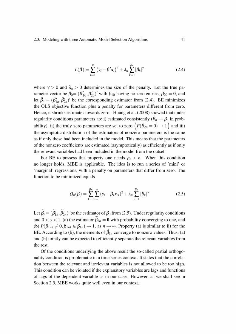
2.3. Modeling with three Automatic Model Selection Algorithms 41
L(β ) =n
∑i=1
(yi−β
′xi)2 +λn
pn
∑k=1|βk|γ (2.4)
where γ > 0 and λn > 0 determines the size of the penalty. Let the true pa-rameter vector be β0= (β ′10,β
′20)′ with β10 having no zero entries, β20 = 0, and
let βn = (β ′1n, β′2n)′ be the corresponding estimator from (2.4). BE minimizes
the OLS objective function plus a penalty for parameters different from zero.Hence, it shrinks estimates towards zero . Huang et al. (2008) showed that underregularity conditions parameters are i) estimated consistently (βn→ βn in prob-ability), ii) the truly zero parameters are set to zero
(P(β2n = 0)→ 1
)and iii)
the asymptotic distribution of the estimators of nonzero parameters is the sameas if only these had been included in the model. This means that the parametersof the nonzero coefficients are estimated (asymptotically) as efficiently as if onlythe relevant variables had been included in the model from the outset.
For BE to possess this property one needs pn < n. When this conditionno longer holds, MBE is applicable. The idea is to run a series of ’mini’ or’marginal’ regressions, with a penalty on parameters that differ from zero. Thefunction to be minimized equals
Qn(β ) =pn
∑k=1
n
∑i=1
(yi−βkxik)2 +λn
pn
∑k=1|βk|γ (2.5)
Let βn= (β ′1n, β′2n)′ be the estimator of β0 from (2.5). Under regularity conditions
and 0 < γ < 1, (a) the estimator β2n = 0 with probability converging to one, and(b) P(β1nk 6= 0, β1nk ∈ β1n)→ 1, as n→ ∞. Property (a) is similar to ii) for theBE. According to (b), the elements of β1n converge to nonzero values. Thus, (a)and (b) jointly can be expected to efficiently separate the relevant variables fromthe rest.
Of the conditions underlying the above result the so-called partial orthogo-nality condition is problematic in a time series context. It states that the correla-tion between the relevant and irrelevant variables is not allowed to be too high.This condition can be violated if the explanatory variables are lags and functionsof lags of the dependent variable as in our case. However, as we shall see inSection 2.5, MBE works quite well even in our context.

42 Chapter 2. Forecasting by Automated Modelling Techniques
QuickNet
QuickNet (QN) resembles an earlier modelling device called RETINA, seePerez-Amaral, Gallo, and White (2003). The idea of RETINA is to find theexplanatory variables that in absolute terms are most strongly correlated with yt .
The most correlated variable is selected first, and the following ones one by onethereafter. QuickNet differs from RETINA in that the set of candidate variablesis different, as is the model selection criterion used for final selection. QuickNetworks as follows. First, the set of candidate variables S, see (2.2), is constructed.The variables have to be such that they show sufficient variation in the sam-ple and are not perfectly linearly correlated; see White (2006) for details. Thisset of candidate variables is also used when Autometrics and MBE are applied.Once this has been done, a predetermined number of variables, q, are added tothe model from the set S, according to the rule that selects the variable with thestrongest (positive or negative) correlation with the residuals of the previouslyestimated model. Then a model selection criterion is applied to choose a sub-set of the q variables. We used 10-fold cross validation as suggested by Hastie,Tibshirani, and Friedman (2009).
We also experiment with a simplified unidirectional version of this method.The variables are selected one at a time as before, but the significance of thethe added variable is tested at each step. Parsimony is appreciated, so the sig-nificance level of the tests is decreased as the number of variables n the modelincreases. Adding variables is terminated at the first non-rejection of the nullhypothesis, so this is a pure specific-to-general strategy. In the empirical sec-tion, we apply this method such that the significance level of the first test in thesequence equals 0.2. Beginning with this value, the significance level is thenhalved at each step. In reporting results in Section 2.5, this method is calledQN-SG. To compare the forecasts of the neural network models to genuinelynonparametric ones, direct Nadaraya-Watson kernel regression forecasts (NP)are generated. Finally, no change forecasts (NC), which forecast that the vari-able of interest takes the same value at any future point in time as it does at thetime of forecasting, are computed and compared with the others.

2.4. Forecasting 43
2.4 Forecasting
Two Ways of Generating Multiperiod Forecasts
There are two main ways of creating multiperiod forecasts. One can either gen-erate the forecasts recursively, or one may apply direct forecasting. In the formercase, one and the same model is used for all forecast horizons. Direct forecastingimplies that a separate model is built for each forecast horizon. In the empiricalsection of the paper we shall compare results from these two approaches. A briefdiscussion of these two techniques follows next.
Recursive Forecasts
In order to illuminate recursive forecasting, consider the model (2.1) withp = q = 1. These restrictions are for notational simplicity only. Assuming theinformation set FT−1 = yT− j, j ≥ 1 is independent of future error terms, theone-period-ahead forecast made at time T equals
yT+1|T = E(yT+1|FT
)= β00 +β01yT +β1(1+ expγ0 + γ1yT)−1.
The corresponding conditional mean yT+2|T , that is, the two-period forecast,becomes
yT+2|T = E(
β00 +β01yT+1 +β1(1+ exp(γ0 + γ1yT+1))−1 + εT+2|FT
)= β00 +β01yT+1|T +β1E
(1+ exp(γ0 + γ1(yT+1|T + εT+1))−1|FT
)= β00 +β01yT+1|T +β1
∫∞
−∞
(1+ exp(γ0 + γ1(yT+1|T + z)))−1φ(z)dz
(2.6)
where φ(z) is the density of the N (0,σ2) random variable. The integral in(2.6) can be computed by numerical integration. Note that it becomes a multipleintegral when the forecast horizon h > 2. It is therefore better to calculate itsvalue by simulation or by bootstrapping the residuals of the model, because thisremains a computationally feasible method even when h > 2. Some authorsbypass this complication altogether by setting εT+1 = 0 in the logistic function,and as a result their forecasts are biased estimates of the conditional mean.
In this work we apply the same bootstrap as in Chapter 1. The bootstrap hasthe advantage over simulation that unconditional heteroskedasticity of unknownform is allowed in the error process. More discussion about recursive forecasting

44 Chapter 2. Forecasting by Automated Modelling Techniques
can be found in Terasvirta (2006), Kock and Terasvirta (2011) or Terasvirta et al.(2010, Chapter 14) among others.
Direct forecasts
In direct forecasting, the conditional mean estimate arises from a different modelfor each time horizon. Given the information set FT , the forecast for T +h madeat T equals
yDT+h|T = gh(yT ,yT−1, ...,yT−p+1)
where gh is a function of yT and its lags. In our case, model selection is madeusing the three aforementioned techniques, but there is a ’gap’ in the modelin that yT+h−1, ...,yT+1 do not enter the equation. The advantage of the directmethod lies in its computational simplicity: no recursions are needed. But then,a separate model has to be specified for each forecast horizon.
Forecasts based on differences and forecast errors
The forecasts based on differences are obtained in the following way. Whenforecasting recursively first differences ∆yt = yt − yt−1 are being modelled andforecast. The p lags of the left hand side variable are thus ∆yt−1, ...,∆yt−p To getan h-periods-ahead forecast, which is of yT+h, the first-difference forecasts haveto be cumulated1:
E(yT+h|FT
)=
h
∑j=1
E(∆yT+ j|FT
)+ yT . (2.7)
The corresponding forecast error is eT+h|T = yT+h−E(yT+h|FT
).
In direct h-periods-ahead forecasting, the variable to be modeled is ∆hyt =yt−yt−h. The p lags of the left-hand side variable are thus ∆hyt−h, ...,∆hyt−h−p+1
and the corresponding forecast of yT+h is E(∆hyT+h|FT
)+ yT . The estimated
model yields direct estimates of the conditional mean.The measure of performance in this work is the root mean square forecast
error (RMSFE). It is calculated for each time series from out-of-sample forecastsfor the forecasting period beginning at T0 and ending at T −hmax, where T is thelast available observation and hmax is the maximum forecast horizon. Thus,
RMSFEh = (T −hmax−T0 +1)−1T−hmax
∑t=T0
e2t+h|t
1/2.
1The unknown E(∆yT+ j|FT
)are of course replaced by their bootstrapped counterparts.

2.5. Results 45
Insanity Filters
Nonlinear models may sometimes generate forecasts that are deemed unrealisticin the light of the hitherto observed values of the time series. This has promptedforecasters to introduce precautions in order to avoid excessive forecast errors.The idea is to replace an unrealistic forecast with a more conventional and be-lievable one. It has been applied, among others, by Swanson and White (1995,1997a,b) who call the procedure the insanity filter, Stock and Watson (1999) andTerasvirta et al. (2005). We shall make use of two insanity filters. The first oneworks as follows: If the h-step ahead predicted change exceeds the maximumh-step change observed during the estimation period, the most recently observedvalue of the variable to be predicted is the forecast. Hence, in the words of Swan-son and White (1995) we “replace craziness by ignorance”. We shall call thisfilter the Swanson and White (SW) filter. In the second filter, the extreme pre-dicted change is replaced by a forecast from our benchmark linear autoregressivemodel: craziness is replaced by linearity.
2.5 Results
The above techniques are applied to the monthly Consumer Price Index (CPI)and unemployment series for the G7 countries as well as the four Scandinaviancountries. Before considering these macroeconomic series a small Monte Carloexperiment is conducted. As mentioned in the introduction, the purpose of thisexercise is to see how the three modelling procedures perform under controlledcircumstances when the data generating process is known and contained in thelinear span of S and thus is possible to select.
General methodology and data
The technique for generating the potential hidden units for the ANN model (2.1)is described in the Appendix. We have modified the original White (2006) tech-nique somewhat to make it more suitable to our modelling problem. For Quick-Net and MBE we used 10-fold cross validation as in Hastie et al. (2009) todetermine the number of hidden units to be included. We also used the hv-CrossValidation procedure of Racine (2000) but this did not improve the results, sothey are omitted. Following the suggestion of White (2006), the maximum num-ber of variables in the ANN models was set to ten.

46 Chapter 2. Forecasting by Automated Modelling Techniques
The macroeconomic series are obtained from the OECD Main Economic In-dicators. Most series begin in the 1960s and end in December 2009 or January2010. The CPI series were transformed to logarithms before modelling them,and the forecast errors discussed in the paper are errors in forecasting the trans-formed series.
Monte Carlo
For our simulation study we chose a strongly nonlinear model from Medeiroset al. (2006). These authors took the well-known annual Wolf’s sunspot numberseries and, after transforming the observations using the Box-Cox transformationas in Ghaddar and Tong (1981), fitted an ANN model (2.1) with two hidden unitsto the transformed series. The model is:
yt =−0.17+0.85yt−1 +0.14yt−2−0.31yt−3 +0.08yt−7
+12.8G1(yt−1)+2.44G2(yt−1)+ εt (2.8)
where the two hidden units are
G1(yt−1) =(
1+ exp(−0.46(0.29yt−1−0.87yt−2 + .40yt−7−6.68)
))−1
and
G2(yt−1) =(1+ exp
(−1.17×10³ (0.83yt−1−0.53yt−2−0.18yt−7 +0.38)
))−1
and εt ∼i.i.d.N(0,1). We generate 500 time series of 600 observations from thismodel. The set of potential variables consists of G1, G2, 1000 other hidden units,and ten lags of yt . The number of variables thus greatly exceeds the numberof observations. The forecast horizons are one, two, and five years, and themaximum number of variables per each selected model equals ten. We reportRMSFE ratios such that the denominator is the RMSFE of forecasts from (2.8),computed from the 500 replications.
Table 2.1 contains these ratios for the recursive forecasts. The first threeentries in the column named DGP contain the RMSFE for the forecasts from thetrue model (2.8). As expected, all RMSFE ratios exceed unity. Autometrics-selected models generate by far the most accurate forecasts of the alternatives

2.5. Results 47
Recursive Hor. DGP AR QN MBE Autom. QN-SG
1 1.82 1.456 1.343 1.730 1.105 1.805NF 2 2.739 1.536 3.282 1.659 1.073 1.568
5 4.172 1.337 9 ·104 1.394 4023 1.283
1 1 1.456 1.513 1.730 1.105 1.855SW 2 1.001 1.536 1.532 1.658 1.074 1.552
5 1.001 1.392 1.218 1.395 1.028 1.269
1 1 1.456 1.322 1.730 1.105 1.776AR 2 1.001 1.536 1.366 1.658 1.074 1.552
5 1.001 1.337 1.214 1.395 1.028 1.269
Table 2.1: Average root mean square forecast error ratios for the recursive forecasts of the simulatedsunspot series. DGP: Data generating process, AR: Autoregression, QN: QuickNet, MBE: Marginal BridgeEstimator, Autom.: Autometrics, QN-SG: Quick-Net specific to general. NF: No Filter (for the DGP theNF subcolumn contains the actual root mean square forecast error from forecasting with the DGP), SW:Swanson-White filter, AR: Insane forecasts replaced by linear autoregressive ones.
Direct Hor. AR QN MBE Autom. QN-SG NP NC
1 1.456 1.343 1.730 1.105 1.805 1.546 3.560NF 2 1.518 9.575 1.549 1.652 1.436 1.332 4.226
5 1.306 1.353 1.241 1.359 1.293 1.124 3.984
1 1.456 1.513 1.730 1.105 1.855 1.658SW 2 1.518 1.52 1.549 1.532 1.733 1.424
5 1.363 1.326 1.241 1.322 1.293 1.124
1 1.456 1.322 1.730 1.105 1.776 1.555AR 2 1.518 1.35 1.549 1.355 1.444 1.335
5 1.306 1.219 1.241 1.246 1.293 1.124
Table 2.2: Average root mean square forecast error ratios for the direct forecasts of the simulatedsunspot series. NP: Non-parametric, NC: No Change forecasts. NF: No Filter, SW: Swanson-White filter,AR: Insane forecasts replaced by linear autoregressive ones.
to the DGP, indicating that the method works well when there is a true modelthat can be selected from the set of variables available for the purpose. The othermethods lead to models whose forecasts are of more or less the same quality. Theforecasts from MBE-selected models do not need filtering but are nevethelessslightly more inaccurate than the other (filtered) ones.
The performance of direct models is reported in Table 2.2. Models selectedby Autometrics no longer generate more accurate forecasts than the other non-linear models. Every possible direct model is misspecified by definition becausethe shortest lag (two-year model) or lags (five-year model) of yt cannot be used,and Autometrics clearly suffers from this. Note the good performance of thenonparametric model forecasting five years ahead. The kernel autoregression

48 Chapter 2. Forecasting by Automated Modelling Techniques
Rec Hor. DGP AR QN MBE Autom. QN-SG
1 3.35 4.53 4.03 4.92 3.68 4.6AR 2 5.18 7.28 6.13 7.68 5.77 7.01
5 5.5 7.28 6.24 7.16 5.49 6.6
Dir Hor. AR QN MBE Autom. QN-SG NP NC
1 4.53 4.03 4.92 3.68 4.6 4.5 6.23AR 2 7.19 6.65 7.54 6.2 6.93 6.67 10.4
5 7.1 6.6 6.79 6.47 7.07 6.15 10.4
Table 2.3: Average ranks based on the absolute forecasts errors. For each procedure for which forecastsare carried out recursively as well as directly the forecasts from the two alternatives are identical at the1-month horizon. Hence, the comparison is only made across the DGP forecasts and the direct forecasts atthe 1-month horizon and by construction the ranks are the same for the recursive counterparts.
seems to make most of the available information, and the forecasts hardly needfiltering. In fact, the SW filter has a negative effect on the accuracy of the fore-casts from this model. As may be expected, the No Change forecast does notperform well in predicting these strongly cyclical realisations.
We also compare the methods by calculating the average ranks of the abso-lute forecast errors. Only the results for the AR filtered forecasts are reportedsince the ranks obtained from the SW filtered ones are similar.
The ranks can be found in Table 2.3. As can be expected from the RMSFEresults, the forecasts from the DGP have the lowest ranks. However, the ranksof the recursive forecasts by Autometrics are not much higher and even as lowas the DGP ones at the five year horizon. Of the remaining neural networkprocedures MBE forecasts have the highest ranks while the No Change forecastsare by far the least accurate overall. This is not surprising due to the cyclicalnature of the series to be forecast. The nonparametric forecasts perform about aswell as the ANN-based procedures at the shortest horizons and better than themat the five year horizon.
Another robust way of considering the results is to use Wilcoxon’s signed-rank test (Wilcoxon (1945)) for comparing forecasts from the DGP with theothers. The null hypothesis is that the absolute forecast error of the DGP andthat of the other model have the same mean whereas the alternative is that thealternative model has a lower mean absolute forecast error. The tests are carriedout separately for each horizon. The results are reported in Table 2.4. A normalapproximation has been used in calculating the p-values. This is appropriate dueto the large number of forecasts (500). Small p-values indicate that the alter-native model produces more accurate forecasts than the DGP. If the alternative

2.5. Results 49
Recursive Hor. AR QN MBE Autom. QN-SG
1 1 1 1 1 1AR 3 1 1 1 1 1
5 1 1 1 0.852 1
Direct Hor. AR QN MBE Autom. QN-SG NP NC
1 1 1 1 1 1 1 1AR 3 1 1 1 1 1 1 1
5 1 1 1 1 1 1 1
Table 2.4: p-values of the Wilcoxon signed-rank test for testing the null of the mean of the forecasterrors from the DGP being equal to the mean of the corresponding forecast error from the model in eachcolumn of the table. The tests are carried out separately at each horizon and the alternative hypothesisis that the model in the table has a lower mean. Top panel: Recursive forecasts. Bottom panel: Directforecasts.
Recursive Total Linear Nonlinear DGP units
QN 9.55 0.348 9.21 1.64MBE 9.22 0.756 8.47 0.77Autom 11 1.5 9.51 3.47QN-GS 5.3 0.324 4.98 1.12
Table 2.5: Average number of variables selected for the recursive forecasts of the CPI based on differ-ences. “Total” indicates total number of variables included, “Linear” indicates the number of linear unitsincluded, “Nonlinear” gives the number of hidden units included, and DGP units gives the number of unitsincluded from the data generating process.
hypothesis is that the forecasts from the DGP have the lowest mean, one simplysubtracts the reported p-values from one and obtains the p-values of this test. Alltests are based on the AR-filtered forecasts2.
As can be seen from Table 2.4, the results in Tables 2.1 and 2.2 accord withthose from the Wilcoxon test. It is not possible to reject the hypothesis thatthe absolute forecast errors of the DGP forecasts and those from the alternativemodel have the same mean if the alternative hypothesis is that the alternativemodel has a lower mean. If the alternative hypothesis is that the DGP forecasterrors have a lower mean, the null of equal means is rejected at a five percentsignificance level with a single exception: the recursive five-year forecasts fromthe Autometrics-selected ANN model.
Table 2.5 offers some background to the results in Tables 2.1 and 2.2. It con-2Alternatively, one could consider the Giacomini-White test (Giacomini and White (2006))
which includes the Diebold-Mariano test (Diebold and Mariano (1995)) as a special case. TheGiacomini-White test, however, relies on a rolling window. The Giacomini-White test was alsocarried out but most often the conclusions were the same as for the Wilcoxon test and so theresults are not reported here.

50 Chapter 2. Forecasting by Automated Modelling Techniques
tains information about the size and variable types in the nonlinear models forrecursive forecasting. The average number of variables in every type of model islarger than the size of (2.8) which is six variables as the intercept is not counted.It is worth noting that Autometrics, while selecting the largest models, picks upelements of the true model more frequently than the other model selection tech-niques. This is probably the most important factor in explaining its success inforecasting. Moreover, Autometrics on average chooses more linear lags than theother models, although fewer than their number in the true model. The averagenumber of linear lags in the other models is rather small. The specific-to-generalQN-SG is clearly more parsimonious than QuickNet, but this result is not in-variant to the choice of significance levels in the test sequence. QuickNet-basedrecursive forecasts are somewhat more accurate than QN-SG ones at one-andfive-year horizons.
Macroeconomic forecasts
The CPI and unemployment series are forecast at the 1, 3, 6, and 12-monthhorizons. The CPI series are transformed into logarithms, and 240 forecastsbased on an expanding window are generated for each horizon3. Forecasts frommodels of differenced series are formed as described in Section 2.4. The poolof variables contains 600 hidden units with p = 6 in (2.1) and the first six linearlags of the dependent variable.
The models are respecified every six months. This is because Autometrics isquite slow: otherwise respecification could easily be done every month. Pretest-ing linearity and letting the nonlinear model selection operate only if the linearityhypothesis was rejected did not on average improve the performance of the non-linear models. This may be due the fact that linear lags are included into the poolof hidden units which makes it possible to select a linear model anyway.
Consumer Price Index
The RMSFE ratios for recursive CPI forecasts from models of differenced se-ries can be found in Table 2.6. The denominator in the RMSFE ratio is now theRMSFE of the recursive linear AR forecasts. It is seen that filtering the fore-casts is necessary. All four model selection techniques lead to ANN models that
3For some of the shorter data sets the number of forecasts is less than 240, because the firstwindow was set to include at least 200 observations.
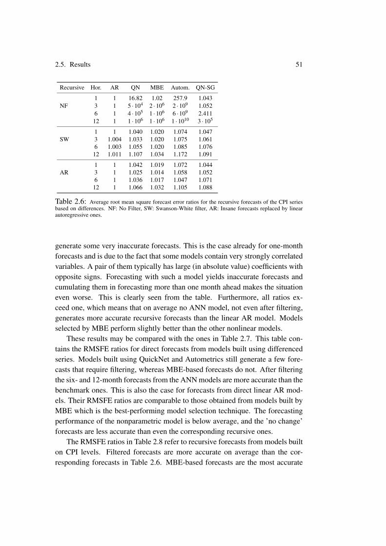
2.5. Results 51
Recursive Hor. AR QN MBE Autom. QN-SG
1 1 16.82 1.02 257.9 1.043NF 3 1 5 ·104 2 ·106 2 ·109 1.052
6 1 4 ·105 1 ·106 6 ·109 2.41112 1 1 ·106 1 ·106 1 ·1010 3 ·105
1 1 1.040 1.020 1.074 1.047SW 3 1.004 1.033 1.020 1.075 1.061
6 1.003 1.055 1.020 1.085 1.07612 1.011 1.107 1.034 1.172 1.091
1 1 1.042 1.019 1.072 1.044AR 3 1 1.025 1.014 1.058 1.052
6 1 1.036 1.017 1.047 1.07112 1 1.066 1.032 1.105 1.088
Table 2.6: Average root mean square forecast error ratios for the recursive forecasts of the CPI seriesbased on differences. NF: No Filter, SW: Swanson-White filter, AR: Insane forecasts replaced by linearautoregressive ones.
generate some very inaccurate forecasts. This is the case already for one-monthforecasts and is due to the fact that some models contain very strongly correlatedvariables. A pair of them typically has large (in absolute value) coefficients withopposite signs. Forecasting with such a model yields inaccurate forecasts andcumulating them in forecasting more than one month ahead makes the situationeven worse. This is clearly seen from the table. Furthermore, all ratios ex-ceed one, which means that on average no ANN model, not even after filtering,generates more accurate recursive forecasts than the linear AR model. Modelsselected by MBE perform slightly better than the other nonlinear models.
These results may be compared with the ones in Table 2.7. This table con-tains the RMSFE ratios for direct forecasts from models built using differencedseries. Models built using QuickNet and Autometrics still generate a few fore-casts that require filtering, whereas MBE-based forecasts do not. After filteringthe six- and 12-month forecasts from the ANN models are more accurate than thebenchmark ones. This is also the case for forecasts from direct linear AR mod-els. Their RMSFE ratios are comparable to those obtained from models built byMBE which is the best-performing model selection technique. The forecastingperformance of the nonparametric model is below average, and the ’no change’forecasts are less accurate than even the corresponding recursive ones.
The RMSFE ratios in Table 2.8 refer to recursive forecasts from models builton CPI levels. Filtered forecasts are more accurate on average than the cor-responding forecasts in Table 2.6. MBE-based forecasts are the most accurate

52 Chapter 2. Forecasting by Automated Modelling Techniques
Direct Hor. AR QN MBE Autom. QN-SG NP NC
1 1 16.82 1.02 257.9 1.043 1.148 1.133NF 3 0.976 2.699 0.9893 2464 1.02 1.074 1.169
6 0.8123 20.77 0.8239 1869 0.8362 0.9335 1.15912 0.7336 3.286 0.7284 20.08 0.7436 0.8203 1.134
1 1 1.040 1.020 1.074 1.047 1.150SW 3 0.976 1.039 0.9893 1.059 1.030 1.081
6 0.8123 0.8452 0.8239 0.8987 0.836 0.933512 0.7336 0.7584 0.7284 0.8355 0.7397 0.8203
1 1 1.042 1.019 1.072 1.044 1.147AR 3 0.976 1.020 0.9893 1.042 1.019 1.075
6 0.8123 0.840 0.8239 0.8819 0.835 0.933512 0.7336 0.7591 0.7284 0.8371 0.7395 0.8203
Table 2.7: Average root mean square forecast error ratios for the direct forecasts of the CPI seriesbased on differences. NF: No Filter, SW: Swanson-White filter, AR: Insane forecasts replaced by linearautoregressive ones.
Recursive Hor. AR QN MBE Autom. QN-SG
1 1.011 1.013 0.977 1.062 1.139NF 3 1.001 20.39 0.9315 6311 1.195
6 0.9728 3 ·105 0.8535 1 ·107 1.22312 0.9372 3 ·106 0.787 3 ·108 1.309
1 1.011 1.013 0.977 1.062 1.139SW 3 1.001 0.9685 0.9314 1.003 1.184
6 0.9728 0.896 0.8532 0.9299 1.18712 0.9372 0.823 0.7871 0.8489 1.185
1 1.011 1.013 0.977 1.062 1.139AR 3 1.001 0.9661 0.9314 1.003 1.181
6 0.9728 0.8923 0.8532 0.9299 1.18712 0.9372 0.8143 0.7871 0.8489 1.167
Table 2.8: Average root mean square forecast error ratios for the recursive forecasts of the CPI se-ries based on levels. NF: No Filter, SW: Swanson-White filter, AR: Insane forecasts replaced by linearautoregressive ones.
ones and models built by QN-SG generate the least accurate recursive forecasts:all ratios remain above one. Recursive linear AR models built on levels aresomewhat superior to the ones built on differences. The RMSFE ratios lie belowone for the two longest horizons but are greater than the corresponding ratios forforecasts from models obtained by MBE, QuickNet and Autometrics.
Table 2.9 contains the RMSFE ratios for direct forecasts from models speci-fied and estimated from the level series. It appears that MBE is the best model-building method when the criterion is the RMSFE. The ratios are even smaller

2.5. Results 53
Direct Hor. AR QN MBE Autom. QN-SG NP NC1 1.011 1.013 0.977 1.062 1.139 16.77 1.133
NF 3 0.9661 0.9418 0.9057 0.9761 1.198 8.037 1.1696 0.9053 3.401 0.8114 0.9982 1.204 5.072 1.15912 0.7771 0.7205 0.6928 0.9416 1.173 3.119 1.1341 1.011 1.013 0.977 1.062 1.139 3.783
SW 3 0.9661 0.9418 0.9057 0.9761 1.198 5.1726 0.9053 0.8305 0.8114 0.954 1.204 4.90712 0.7771 0.7205 0.6928 0.9416 1.173 3.1191 1.011 1.013 0.977 1.062 1.139 3.675
AR 3 0.9661 0.9418 0.9057 0.9761 1.198 5.1366 0.9053 0.8303 0.8114 0.9564 1.204 4.90412 0.7771 0.7205 0.6928 0.9416 1.173 3.119
Table 2.9: Average root mean square forecast error ratios for the direct forecasts of the CPI series basedon levels. NF: No Filter, SW: Swanson-White filter, AR: Insane forecasts replaced by linear autoregressiveones.
than the ones found in Tables 2.6–2.8. Direct models selected by QuickNetalso perform better than the recursive ones, whereas the same cannot be saidof models based on Autometrics or QN-SG. In the light of these results, goingfrom specific to general and back again (QuickNet) is a better idea than goingfrom specific to general only (QN-SG), but this finding cannot be generalized. Itmay be noted that the nonparametric model built on levels generates much lessaccurate forecasts than the same model estimated from differenced series. ItsRMSFE ratios are remarkably larger than any other ratio. Summing up, it seemsthat direct forecasts are on average more accurate than the recursive ones. Ex-ceptions do exist: compare Autometrics-based six- and 12-month RMSFE ratiosin Tables 2.8 and 2.9. It should be pointed out that these results are aggregateones and do not necessarily hold for all 11 countries.
As was the case for the simulation study we also compare the forecast per-formance of the methods applied by considering their ranks. This is done forall countries and forecast horizons. Furthermore, forecasts from models built ondifferences and the ones based on levels are included in the same comparison.
The results can be found in Table 2.10. At the 1-month horizon absoluteforecast errors from the ANN procedures have ranks very close to each other,which is in accordance with the findings from Tables 2.6-2.9. The nonpara-metric and No Change forecasts have considerably higher ranks than the otherprocedures. This is true for the forecasts based on differences as well as theones based on levels. In particular the high ranks for the nonparametric fore-casts based on levels are no surprise in the light of the high relative RMSFE in

54 Chapter 2. Forecasting by Automated Modelling Techniques
Rec Diff Hor. AR QN MBE Autom. QN-SG
1 6.53 6.62 6.57 6.89 6.71AR 3 11.8 11.9 11.7 12 12.4
6 12.9 12.8 12.7 12.8 13.512 14.5 14.7 14.4 15.1 15.1
Dir Diff Hor. AR QN MBE Autom. QN-SG NP NC
1 6.53 6.62 6.57 6.89 6.71 8.2 7.38AR 3 11 11.2 11.2 11.1 11.3 13.8 13.6
6 8.95 9.25 9.05 9.85 9.37 12.5 14.212 8.9 8.66 8.65 9.44 8.52 11.4 14.4
Rec Level Hor. AR QN MBE Autom. QN-SG
1 6.62 6.32 6.21 6.49 7.68AR 3 11.7 10.6 10.7 10.8 14.1
6 12.1 10.8 10.7 10.5 14.912 12.3 10.2 10.5 9.89 14.9
Dir Level Hor. AR QN MBE Autom. QN-SG NP NC
1 6.62 6.32 6.21 6.49 7.68 7.97 7.38AR 3 10.5 10.3 10.1 10.7 14.3 17.7 13.6
6 10.5 9.95 9.73 10.8 15 22 14.212 8.91 9.32 8.94 9.89 14.5 21.6 14.4
Table 2.10: Average ranks based on the absolute forecasts errors. For each procedure for which fore-casts are carried out recursively as well as directly the forecasts from the two alternatives are identical at the1-month horizon. Hence, the comparison is only made across the direct forecasts at the 1-month horizonand by construction the ranks are the same for the recursive counterparts.
Table 2.9. In general, the direct methods have the lowest average ranks. This isthe case in particular for the forecasts based on the differences of the series. Theoverall winner at the 12-month horizon is the QN-SG method based on differ-ences while the MBE-based forecasts come in second. This again agrees withthe results reported in Tables 2.6-2.9.
Similarly to the simulated example, we conduct Wilcoxon’s signed-rank testfor pairs of absolute forecast error series. The benchmark, the recursive linearAR forecast based on differences, is always one of the forecasts in the pair. Asalready discussed, the null hypothesis of the test is that the means of the absoluteforecast errors are equal, and the alternative is that the absolute forecast errorsof the ’other model’ have the smaller mean of the two. The upper panel ofTable 2.11 contains p-values of the test for recursive forecasts from differencedmodels. Most of them are close to one, which means that the null hypothesisis rejected in the opposite direction. This accords with the information in Table2.6, where all RMSFE ratios were greater than one. The MBE-based forecasts

2.5. Results 55
Recursive Hor. QN MBE Autom. QN-SG
1 0.998 0.778 1 1AR 3 0.963 0.0582 0.982 1
6 0.949 0.266 0.995 112 1 1 1 1
Direct Hor. AR QN MBE Autom. QN-SG NP NC
1 0.998 0.778 1 1 1 1AR 3 0 0.011 1 ·10−5 1 ·10−5 0.005 1 1
6 0 0 0 0 0 0 112 0 0 0 0 0 0 0.968
Table 2.11: p-values of the Wilcoxon signed-rank test for testing the null of the mean of the forecasterrors from recursive forecasts of the CPI series from the linear AR estimated on differences is equal tothe mean of the corresponding forecast error from the model in each column of the table. The tests arecarried out separately at each horizon and the alternative hypothesis is that the model in the table has alower mean. Top panel: Models estimated recursively on differences. Bottom panel: Models estimateddirectly on differences.
at horizons up to six months constitute the only exception.The lower panel contains the p-values for direct forecasts. They are mostly
close to zero for long forecasting horizons. The no change forecast is the onlyexception: all p-values are large. Direct forecasts can thus be deemed superiorto recursive ones when the models are built on differenced CPI-series. Thisstrengthens conclusions that emerge from Tables 2.6 and 2.7.
Table 2.12 contains p-values of the same test and null hypothesis when theforecasts are obtained using models built on CPI series in levels. Results in theupper panel show that the null hypothesis is rejected in favour of the recursivelinear AR forecasts based on differences when compared to the model selectedby QN-SG. The other methods generate ANN models that yield more accuraterecursive forecasts than the linear AR model (p-values are close to zero) or fore-casts for which the null hypothesis is not rejected (QuickNet and Autometricsone-month forecasts). The lower panel shows that QN-SG-based direct mod-els do not perform well either. The same can be said about the nonparametricmodel and the ’no change’ forecasts. Considering all four horizons at once, MBEemerges as the best-performing model selection criterion for direct models whenWilcoxon’s test is used as the yardstick.
As in the simulated example, it is interesting to see whether the size of themodel and the accuracy of the forecasts from it have to do with each other. Table2.13 contains information about the size and composition of models based ondifferenced series. When forecasting recursively, it is seen from the left panel

56 Chapter 2. Forecasting by Automated Modelling Techniques
Recursive Hor. QN MBE Autom. QN-SG
1 0.160 1 ·10−4 0.171 1AR 3 1 ·10−8 0 4 ·10−6 1
6 0 0 0 112 0 0 0 1
Direct Hor. AR QN MBE Autom. QN-SG NP NC
1 1 0.160 1 ·10−4 0.171 1 1 1AR 3 0 0 0 4 ·10−8 1 1 1
6 0 0 0 0 1 1 112 0 0 0 0 1 1 0.968
Table 2.12: p-values of the Wilcoxon signed-rank test for testing the null of the mean of the forecasterrors from recursive forecasts of the CPI series from the linear AR estimated on differences is equal to themean of the corresponding forecast error from the model in each column of the table. The tests are carriedout separately at each horizon and the alternative hypothesis is that the model in the table has a lower mean.Top panel: Models estimated recursively on levels. Bottom panel: Models estimated directly on levels.
Recursive Total Linear Nonlinear
QN 6.35 0.298 6.05MBE 5.51 0.818 4.69AM 15.5 0.393 15.1QN-SG 4.03 0.195 3.83
Direct MBE Total Linear Nonlinear
1 mth 5.51 0.818 4.693 mths 5.48 2.45 3.036 mths 5.29 3.55 1.7412 mths 2.69 1.72 0.964
Table 2.13: Left panel: Average number of variables selected for the models generating recursiveforecasts of the CPI based on differences. “Total” indicates total number of variables included, “Linear”indicates the number of linear units included, and “Nonlinear” gives the number of hidden units included.Right panel: Average number of variables selected for the direct forecasts of the CPI based on differencesby MBE.
that QN-SG selects the most parsimonious models which do not, however, yieldthe most accurate forecasts. MBE selects somewhat less parsimonious modelsthat on average yield the most accurate recursive forecasts. It also chooses thelargest fraction of linear lags, although their average number remains below one.Models selected by Autometrics are by far the largest ones. There does not seemto be a clear connection between the model size and forecast accuracy.
The right-hand panel of Table 2.13 contains the average size and compositionof models based on differenced series and selected by MBE for direct forecast-ing. The average number of variables is halved when one moves from six- to12-month models, whereas the share of linear lags of the total increases up tosix-month models and remains about the same for 12-month ones.
Table 2.14 contains the same information for models built on levels. Allmethods now select more linear variables than in the previous case. QN-SG isstill the most parsimonious technique, and even QuickNet selects fewer vari-

2.5. Results 57
Recursive Total Linear Nonlinear
QN 5.35 1.09 4.27MBE 7.19 5.64 1.55AM 19.1 1.34 17.7QN-SG 1.39 1 0.386
Direct MBE Total Linear Nonlinear
1 mth 7.19 5.64 1.553 mths 7.24 5.74 1.496 mths 7.42 6 1.4212 mths 7.21 6 1.21
Table 2.14: Left panel: Average number of variables selected for the models generating recursiveforecasts of the CPI based on levels. “Total” indicates total number of variables included, “Linear” indicatesthe number of linear units included, and “Nonlinear” gives the number of hidden units included. Rightpanel: Average number of variables selected for the direct forecasts of the CPI based on levels by MBE.
ables than MBE. As Tables 2.9 and 2.12 indicate, forecasts from MBE are stillthe most accurate ones on average. The use of Autometrics leads to largest mod-els. They perform better than QN-SG-selected models but less well than onesspecified using MBE. The right panel of table 2.14 shows that MBE select a largenumber of linear lags for all direct models. In fact, every MBE-model built forthe two longest horizons contains all six lags and only a small number of hiddenunits. A comparison of the RMSFE ratios in Tables 2.6 and 2.8 on the one handand Tables 2.7 and 2.9 on the other (indirectly) suggests that direct models basedon level data and selected by MBE may be slightly superior to the same type ofmodel, selected by the same technique, but based on differenced series. Whetheror not this is due to the larger amount of linear lags in the former models is notclear, however.
Individual countries
To shed light on some of the cross-country variation in the results thatcannot be seen in the summary tables we now consider results forsome individual countries, Italy, Japan, and the US. They are selectedbecause there are interesting differences between them. The remain-ing country-specific RMSFE are available at http://econ.au.dk/
research/research-centres/creates/research/research-papers/
supplementary-downloads/rp-2011-27/.Tables 2.15 and 2.16 show the RMSFE ratios for the US CPI forecasts based
on differences (only the results for the AR-filter are presented). It is seen that itis indeed possible to improve upon the linear AR model even when forecastingrecursively, although this is not true for all three methods. In fact, only MBEoutperforms the linear autoregression at all horizons, which again indicates itmay be superior to QuickNet and Autometrics in forecasting the CPI series. The

58 Chapter 2. Forecasting by Automated Modelling Techniques
US Recursive Hor. AR QN MBE Autom. QN-SG
1 1 1.03 0.9803 1.044 1.011AR 3 1 0.9811 0.9722 1.003 1.034
6 1 0.9836 0.9388 0.9769 1.00612 1 1.017 0.9484 1.033 1.058
Table 2.15: Average root mean square forecast error ratios for the recursive forecasts of the US CPIseries based on differences. AR: Insane forecasts replaced by linear autoregressive ones.
US Direct Hor. AR QN MBE Autom. QN-SG NP NC
1 1 1.03 0.9803 1.044 1.011 1.044 1.221AR 3 0.9952 0.9742 0.9988 0.9298 0.9403 0.9417 1.179
6 0.8312 0.8749 0.8332 0.8656 0.8825 0.8098 1.22412 0.9483 1.014 0.9145 0.9856 0.9501 0.8423 1.598
Table 2.16: Average root mean square forecast error ratios for the direct forecasts of the US CPI seriesbased on differences. AR: Insane forecasts replaced by linear autoregressive ones.
Wilcoxon tests were also carried out on the individual countries. Based on these,the above findings are significant since at no horizon does one observe a higherp-value than 0.044 when testing the AR forecasts against the recursive MBEones.
On average MBE selects seven variables of which 3.38 are linear lags whenforecasting recursively. It is more parsimonious and includes a higher numberof linear lags than the other procedures.
A comparison of Tables 2.15 and 2.16 shows that for the US the the recursiveforecasts are less accurate than the corresponding direct ones. The differences inthe RMSFE are, however, less pronounced than in Tables 2.6 and 2.7. The find-ing that the direct forecasts are more accurate than the recursive ones is uniformacross all countries. All ANN models, independent of the variable selection pro-cedure, work well in direct forecasting. However, for the US they are at thelongest horizons outperformed by the nonparametric model and perform lesswell than they do in general. For the direct forecasts MBE is again the most par-simonious procedure whereas Autometrics on average selects the largest models.MBE-based models also contain the largest number of linear units.
The averaged results for the forecasts based on levels also sometimes hidedifferences between the individual countries. To illustrate this, Tables 2.17 and2.18 present RMSFE ratios for Italy, Japan, and the US (only the results basedon the AR-filter are shown). Table 2.17 shows that there can be considerablevariation in the performance of the variable selection procedures. MBE is the

2.5. Results 59
ITA Recursive Hor. AR QN MBE Autom. QN-SG
1 1.002 1.165 0.9263 1.603 1.757AR 3 1.055 1.188 0.8965 1.629 1.955
6 1.135 1.252 0.9073 1.677 2.06712 1.195 1.264 0.8355 1.715 1.855
JP Recursive Hor. AR QN MBE Autom. QN-SG
1 0.9667 1.02 0.9885 1.069 1.021AR 3 0.9188 0.9652 0.9612 0.8725 0.9721
6 0.7846 0.8702 0.8419 0.6776 0.880712 0.6717 0.755 0.7242 0.5016 0.7644
US Recursive Hor. AR QN MBE Autom. QN-SG
1 0.9999 1.008 0.9477 0.9458 1.088AR 3 0.9961 0.87 0.9152 0.9035 0.9962
6 0.9877 0.7469 0.8597 0.8102 0.950912 0.9633 0.6898 0.9324 0.8573 1.125
Table 2.17: Average root mean square forecast error ratios for the recursive forecasts of the CPI seriesbased on levels. AR: Insane forecasts replaced by linear autoregressive ones.
most stable procedure and the only one which has RMSFE ratios below unityfor all three countries at all horizons4, but for each country a different variableselection procedure is dominant. The relative stability of MBE is most likely dueto the fact that for all three countries this procedure selects the largest number oflinear units. For Italy and the US it includes all six linear units and for Japan itchooses a purely linear model every time (though not the AR(6)). Nevertheless,MBE is outperformed by Autometrics which generally chooses only a smallfraction of linear lags. However, MBE includes unusually few linear units (3.6)for Japan, so it may still argued that models with a high number of linear unitscombined with a few nonlinear ones perform well on average.
A comparison of the results in Table 2.17 with the ones in Table 2.18 in-dicates that that the direct forecasts are superior to their recursive counterparts.This accords with the overall results. Moreover, the nonparametric model gener-ates very inaccurate forecasts for these three countries, which is also in line withthe general results. The direct MBE forecasts again have RMSFE ratios belowunity. The performance of Autometrics varies quite remarkably. In forecasting
4Recall, however, that the benchmark is the AR(6) model forecasted recursively based ondifferences of the time series. But even then, it still illustrates the rather stable performance ofMBE. Its relative RMSFE are actually below one for the recursive level based forecasts for allcountries at all horizons except for the UK and Denmark for which the 1-month forecasts haveratios above one.

60 Chapter 2. Forecasting by Automated Modelling Techniques
ITA Direct Hor. AR QN MBE Autom. QN-SG NP NC
1 1.002 1.165 0.9263 1.603 1.757 0.9978 1.689AR 3 0.9942 1.091 0.875 1.423 1.977 13.64 1.943
6 0.9135 1.01 0.8358 1.428 1.949 8.529 1.94212 0.7215 0.8067 0.7564 1.571 1.772 4.438 1.733
JP Direct Hor. AR QN MBE Autom. QN-SG NP NC
1 0.9667 1.02 0.9885 1.069 1.021 4.768 0.9762AR 3 0.883 0.925 0.9675 0.8878 0.9711 4.708 0.872
6 0.7352 0.8424 0.7352 0.7064 0.8715 2.999 0.66212 0.5334 0.6727 0.5334 0.5289 0.699 1.591 0.4879
US Direct Hor. AR QN MBE Autom. QN-SG NP NC
1 0.9999 1.008 0.9477 0.9458 1.088 0.9979 1.221AR 3 0.9994 0.8962 0.9212 0.9275 1.014 1.883 1.179
6 1.007 0.7585 0.8741 0.9568 0.9696 4.698 1.22412 1.032 0.7579 0.9107 0.9179 1.147 4.062 1.598
Table 2.18: Average root mean square forecast error ratios for the direct forecasts of the CPI seriesbased on levels. AR: Insane forecasts replaced by linear autoregressive ones. The NC forecasts are notfiltered.
12 months ahead, Autometrics-based forecasts are an excellent choice for Japan,a mediocre one for the US, and are definitely not to be recommended for fore-casting the Italian CPI. The situation is the same if the recursive forecasts inTable 2.17 are considered. Autometrics-based forecasts are much better than therecursive AR ones for Japan, except at the one-month horizon, still acceptablefor the US, and very inaccurate for Italy.
Results on forecasting the CPI series sugest that forecasts based on levels aresuperior to their counterparts based on differences. Furthermore, direct forecast-ing is preferable to recursive forecasts and MBE is the most stable forecastingprocedure. This last observation may be attributed to the high number of lin-ear units MBE includes and which it supplements with a few relevant nonlinearunits.
Unemployment
A common feature of results on forecasting unemployment rate series with thoseon forecasting CPI series is the appearance of some vastly inaccurate forecastsand the consequent need for filtering. This is first seen from Table 2.19 thatcontains the RMSFE ratios for recursive forecasts when the models are built ondifferenced series. For filtered foreacsts, all ratios still lie above one. Models

2.5. Results 61
Recursive Hor. AR QN MBE Autom. QN-SG
1 1 1.124 1.005 2 ·109 1.045NF 3 1 97.78 1.001 7 ·109 1.054
6 1 3333 1.003 1 ·1010 1.05112 1 5 ·104 1.006 1 ·1010 1.026
1 1 1.090 1.006 1.216 1.079SW 3 1.004 1.081 1.007 1.239 1.073
6 1.004 1.058 1.008 1.26 1.05612 1.001 1.026 1.008 1.221 1.026
1 1 1.068 1.005 1.161 1.049AR 3 1 1.07 1.002 1.152 1.058
6 1 1.05 1.004 1.142 1.05112 1 1.021 1.006 1.092 1.025
Table 2.19: Average root mean square forecast error ratios for the recursive forecasts of the unemploy-ment series based on differences. NF: No Filter, SW: Swanson-White filter, AR: Insane forecasts replacedby linear autoregressive ones.
Direct Hor. AR QN MBE Autom. QN-SG NP NC
1 1 1.124 1.005 2 ·109 1.045 0.9999 1.109NF 3 0.9979 59.88 1.024 7 ·106 1.063 1.024 1.167
6 1.002 1.133 1.031 2 ·109 1.133 1.046 1.14812 1.031 250.1 1.054 2 ·108 1.197 1.091 1.055
1 1 1.090 1.006 1.216 1.079 1.013SW 3 1.001 1.060 1.028 1.197 1.062 1.022
6 1.002 1.104 1.030 1.196 1.116 1.04612 1.030 1.101 1.049 1.223 1.128 1.080
1 1 1.068 1.005 1.161 1.049 0.9999AR 3 0.9979 1.053 1.025 1.184 1.058 1.023
6 1.002 1.101 1.028 1.195 1.113 1.04212 1.031 1.109 1.047 1.215 1.138 1.082
Table 2.20: Average root mean square forecast error ratios for the direct forecasts of the unemploymentseries based on differences. NF: No Filter, SW: Swanson-White filter, AR: Insane forecasts replaced bylinear autoregressive ones.
selected by MBE appear to lead to the most accurate nonlinear forecasts, andthey do not need filtering. Autometrics-selected models are, even after filtering,the most inaccurate ones. Table 2.20 indicates that on average, direct forecast arenot superior to recursive ones. This is true for both linear and nonlinear forecasts.Nonparametric forecasts do not require much filtering but are less accurate thanthe ones from the MBE-forecasts.
In the case of unemployment series, the models built on levels do not produceforecasts superior to their counterparts from models based on differences. Table

62 Chapter 2. Forecasting by Automated Modelling Techniques
Recursive Hor. AR QN MBE Autom. QN-SG
1 0.9994 2 ·105 1.007 1.302 1.048NF 3 1.010 3 ·105 1.028 1 ·108 1.076
6 1.024 5 ·106 1.041 8 ·108 1.08712 1.016 9 ·106 1.036 1 ·109 1.065
1 0.9994 1.064 1.007 1.148 1.048SW 3 1.01 1.079 1.027 1.147 1.076
6 1.018 1.106 1.036 1.135 1.08712 1.011 1.085 1.030 1.098 1.061
1 0.9994 1.067 1.007 1.146 1.048AR 3 1.010 1.080 1.027 1.150 1.076
6 1.024 1.108 1.042 1.135 1.08712 1.016 1.093 1.034 1.104 1.061
Table 2.21: Average root mean square forecast error ratios for the recursive forecasts of the unemploy-ment series based on levels. NF: No Filter, SW: Swanson-White filter, AR: Insane forecasts replaced bylinear autoregressive ones.
2.21 contains the RMSFE ratios for recursive forecasts. Again, MBE-selectedmodels seem to generate more accurate forecasts than the others, whereas modelselection using Autometrics leads to the most inaccurate forecasts. The moststriking feature of Table 2.22 is that the nonparametric forecasts, which need nofiltering, are nevertheless on average distinctly more inaccurate than forecastsgenerated by any other model or method. It can also be noted that direct lin-ear forecasts from linear AR models built on untransformed series have RMSFEratios close to one, while no filtering has been necessary. The ’no change’ fore-casts are somewhat less accurate than the ones generated by QuickNet-selectedmodels but better than Autometrics-ones.
Table 2.23 contains the average ranks of the models based on the absoluteforecast errors. In this comparison forecasts from Autometrics-selected modelshave the highest ranks among the ANN models. In accordance with Tables 2.19-2.22, MBE is the best performing ANN selection method. However, none ofthem has a lower average rank than the linear AR model. The performance ofthe nonparametric forecasts is highly dependent on whether the models are builton differences or levels. In the former case the ranks are much lower than in thelatter, which are by far the highest overall. This accords with the RMSFE resultsin Table 2.22.
Table 2.24 contains p-values of Wilcoxon’s signed-rank test of absolute fore-cast errors for AR-filtered forecasts from models based on differenced unem-ployment series. The null hypothesis of equal means is mostly rejected (the

2.5. Results 63
Direct Hor. AR QN MBE Autom. QN-SG NP NC
1 0.9994 2 ·105 1.007 1.302 1.048 1.514 1.109NF 3 1.006 8.759 1.033 2760 1.068 1.507 1.167
6 1.005 1.327 1.045 1.995 1.084 1.499 1.14812 1.008 29.72 1.056 3.201 1.040 1.354 1.055
1 0.9994 1.064 1.007 1.148 1.048 1.514SW 3 1.006 1.08 1.033 1.195 1.068 1.503
6 0.999 1.138 1.039 1.261 1.084 1.49512 1.005 1.063 1.051 1.202 1.04 1.332
1 0.9994 1.067 1.007 1.146 1.048 1.514AR 3 1.006 1.072 1.033 1.196 1.068 1.503
6 1.005 1.133 1.044 1.257 1.084 1.49512 1.008 1.055 1.054 1.203 1.04 1.333
Table 2.22: Average root mean square forecast error ratios for the direct forecasts of the unemploymentseries based on levels. NF: No Filter, SW: Swanson-White filter, AR: Insane forecasts replaced by linearautoregressive ones.
Rec Diff Hor. AR QN MBE Autom. QN-SG
1 6.58 6.89 6.77 7.17 6.84AR 3 11.1 11.9 11.2 12.2 12
6 10.9 11.8 11 12.2 1212 11.1 11.7 11.3 12.2 11.9
Dir Diff Hor. AR QN MBE Autom. QN-SG NP NC
1 6.58 6.89 6.77 7.17 6.84 6.52 5.98AR 3 11 11.9 11.6 12.4 11.7 11.6 12.6
6 10.8 12 11.3 12.3 11.9 11.2 12.912 11.4 12 11.3 12.7 12.1 12.2 12.4
Rec Level Hor. AR QN MBE Autom. QN-SG
1 6.36 6.91 6.45 7.22 6.89AR 3 11 11.9 11.3 12.7 12.2
6 11 12.2 11.3 12.8 12.212 10.8 12.1 11.2 12.7 12.1
Dir Level Hor. AR QN MBE Autom. QN-SG NP NC
1 6.36 6.91 6.45 7.22 6.89 9.23 5.98AR 3 10.8 11.7 11.2 13.1 11.8 15.5 12.6
6 10.5 11.9 11 13.6 12 15.7 12.912 10.7 11.6 11.3 13.1 11.3 15 12.4
Table 2.23: Average ranks based on the absolute forecast errors. For each procedure for which forecastsare carried out recursively as well as directly the forecasts from the two alternatives are identical at the 1-month horizon. Hence, the comparison is only made across the direct forecasts at the 1-month horizon andby construction the ranks are the same for the recursive counterparts.

64 Chapter 2. Forecasting by Automated Modelling Techniques
Recursive Hor. QN MBE Autom. QN-SG
1 1 0.99 1 1AR 3 1 0.645 1 1
6 1 0.962 1 112 1 0.999 1 1
Direct Hor. AR QN MBE Autom. QN-SG NP NC
1 1 0.990 1 1 0.332 1AR 3 0.226 1 0.999 1 1 1 1
6 0.367 1 0.999 1 1 0.991 112 1 1 1 1 1 1 1
Table 2.24: p-values of the Wilcoxon signed-rank test for testing the null of the mean of the forecasterrors from recursive forecasts of the unemployment series from the linear AR estimated on differences isequal to the mean of the corresponding forecast error from the model in each column of the table. The testsare carried out separately at each horizon and the alternative hypothesis is that the model in the table hasa lower mean. Top panel: Models estimated recursively on differences. Bottom panel: Models estimateddirectly on differences.
p-value is close to unity) in favour of the linear recursive AR absolute forecasterrors having a smaller mean than the ones from the other model. MBE fore-casts three months ahead are the only ANN-exception. For direct linear three-and six-month forecasts the null hypothesis of equal means is not rejected either.
Table 2.25 contains the same information with the difference that the al-ternative model is built on levels instead of differences. In this case, the nullhypothesis is never rejected for MBE-based direct models, but it turns out that atlongest horizons, direct linear AR forecasts have smaller absolute errors than therecursive AR ones (the corresponding p-values in Table 2.25 are close to zero).The result for 12-month forecasts requires an explanation. In Table 2.22, the 12-month RMSFE ratio of the direct linear AR forecasts equals 1.008, which doesnot indicate superiority of these forecasts over the recursive linear ones. Evenafter filtering, the direct linear 12-month model generates, however, a couple oflarge absolute forecast errors. This has a considerable effect on the RMSFE buta lesser one on the signed-rank statistic, in which the size of a particular errorweighs less than in the RMSFE. The direct 12-month AR forecasts do have asmaller RMSFE ratio than the other methods in Table 2.22, which is in accordwith the information in Table 2.25.
Statistics on the size and composition of the ANN models for forecastingbased on the differenced unemployment series can be found in Table 2.26. Whenforecasting recursively MBE generates the smallest models and Autometrics thelargest ones. QuickNet and QN-SG lie in between. Most of the selected variables

2.5. Results 65
Recursive Hor. QN MBE Autom. QN-SG
1 1 0.823 1 1AR 3 1 0.999 1 1
6 1 0.999 1 112 1 0.723 1 1
Direct Hor. AR QN MBE Autom. QN-SG NP NC
1 0.333 1 0.823 1 1 1 1AR 3 0.204 1 0.764 1 1 1 1
6 0.003 1 0.404 1 1 1 112 3 ·10−6 0.990 0.148 1 0.828 1 1
Table 2.25: p-values of the Wilcoxon signed-rank test for testing the null of the mean of the forecasterrors from recursive forecasts of the unemployment series from the linear AR estimated on levels is equalto the mean of the corresponding forecast error from the model in each column of the table. The tests arecarried out separately at each horizon and the alternative hypothesis is that the model in the table has alower mean. Top panel: Models estimated recursively on levels. Bottom panel: Models estimated directlyon levels.
Recursive Total Linear Nonlinear
QN 6.62 0.0569 6.56MBE 3.66 0.115 3.55AM 13.7 0.172 13.5QN-SG 6.12 0.0569 6.06
MBE Total Linear Nonlinear
1 mth 3.66 0.115 3.553 mths 2.88 0.295 2.596 mths 2.58 0.227 2.3512 mths 2.49 0.0556 2.43
Table 2.26: Left panel: Average number of variables selected for the models gnerating recursive fore-casts of the unemployment series based on differences. “Total” indicates total number of variables included,“Linear” indicates the number of linear units included, and “Nonlinear” gives the number of hidden unitsincluded. Right panel: Average number of variables selected for the direct forecasts of the unemploymentbased on differences by MBE.
are hidden units. The average size of the MBE-based direct models decreasesslightly with the forecasting horizon. It appears that there is positive correla-tion with the size of the model and its forecasting performance. In Table 2.19and 2.20 models selected by MBE have the smallest RMSFE ratios, whereasAutometrics-based models have the largest ones. Models chosen using Quick-Net and QN-SG lie in the middle.
Table 2.27 contains the same statistics for models based on levels. QN-SGnow produces the most parsimonious models when forecasting recursively, andeven QuickNet-based models have a smaller average size than the ones chosenby MBE. The share of linear lags is now appreciably greater than in Table 2.26,and this is the case for all four procedures. Autometrics selects the largest directmodels, whose average size is practically the same as it is in the models forrecursive forecasting. It appears that in this case, leaving out lags does not affect

66 Chapter 2. Forecasting by Automated Modelling Techniques
Recursive Total Linear Nonlinear
QN 5.02 1 4.02MBE 6.08 5.23 0.848AM 13.6 1.42 12.2QN-SG 2.98 1 1.98
MBE Total Linear Nonlinear
1 mth 6.08 5.23 0.8483 mths 6.03 5.31 0.7236 mths 5.89 5.29 0.612 mths 5.12 4.34 0.782
Table 2.27: Left panel: Average number of variables selected for the models generating recursiveforecasts of the unemployment series based on levels. “Total” indicates total number of variables included,“Linear” indicates the number of linear units included, and “Nonlinear” gives the number of hidden unitsincluded. Right panel: Average number of variables selected for the direct forecasts of the unemploymentseries based on levels by MBE.
the average size of the model.The correlation between the size of the model and the accuracy of the fore-
casts is weaker than in the previous case. A look at Table 2.21 shows that MBE-selected models still have the smallest RMSFE ratios, although they do not havethe smallest size. Note, however, that they contain the largest number of lin-ear lags, which may have affected the outcome. The position of Autometrics isunchanged: largest models and largest RMSFE ratios.
All models for direct forecasting contain more linear terms when the modelsare in levels than when they are in differences. They share this feature with thecorresponding models built for forecasting the CPI.
Individual countries
The average results for the unemployment series are indicative of the re-sults for the individual countries. No large differences can be found onthe country level. However, to illustrate that not all relative RMSFEratios are close to unity we discuss a few individual country results.The tables with the relative RMSFE for each individual country canbe found at http://econ.au.dk/research/research-centres/creates/research/research-papers/supplementary-downloads/rp-2011-27/.
For example the direct forecasts on the differences of the Italian unemploy-ment series are around ten percent more precise than the recursive forecasts fromthe linear autoregression. Similarly to the average results MBE delivers the mostaccurate forecasts of the ANN procedures while Autometrics is the most impre-cise in particular at the short horizons. In fact these two observations are bothvery stable across all eleven countries emphasizing the fact that the average re-sults reflect the results for the individual countries rather well.
The direct forecasts on the levels of the German unemployment series are

2.6. Conclusions 67
another example of a country for which it is possible to outperform the recursivelinear autoregressive model on the differences. These forecasts are also an in-stance of a series for which the SW-filter produces more accurate forecasts thanthe AR-filter. MBE is again the most successful nonlinear model.
2.6 ConclusionsIn this paper we consider macroeconomic forecasting with a flexible nonlinearmodel, the single-hidden layer feedforward neural network model that is a uni-versal approximator. We apply the idea of White (2006) of transforming thespecification and estimation problem of this model to a linear model specifica-tion problem. This leads to a situation in which the number of candidate vari-ables to choose among vastly exceeds the number of observations. Three mod-elling techniques, White’s QuickNet among them, that can handle this difficultyare compared and the models selected are used for forecasting.
The benchmark in our forecast comparisons is, with one exception, the linearAR model with recursive forecasts. It turns out to be difficult to improve upon itsforecasting precision using recursive forecasting, while the direct method seemsto be a more successful approach. It appears that the Marginal Bridge Estimatorof Huang et al. (2008) yields the best performing ANN models overall, but theresults do vary from one country to the other. Autometrics of Doornik (2009) se-lects models with excellent forecasting performance when there is a well-fittingmodel to be discovered but does poorly when no potential model fits the datawell. QuickNet selects models whose average forecasting performance lies be-tween that of the two others. Parsimony plays a role since MBE often selectsmodels with the fewest variables of the available alternatives. The purely non-parametric model generates relatively accurate forecasts for inflation series butis much less successful in forecasting unemployment rates. The performance ofthe models may also vary as a function of the forecasting horizon.
All three techniques often produce models that yield some very erroneousor ’insane’ forecasts, which makes filtering them necessary. The two insanityfilters considered in this paper perform almost equally well, although the ARfilter may have a slight edge over the filter that Swanson and White (1995) intro-duced. Multicollinearity is the main reason for insane forecasts, and it might bea good idea to develop all three modelling strategies further in order to reducethe probability of the outcomes in which the final model contains very stronglylinearly correlated variables.

68 Chapter 2. Forecasting by Automated Modelling Techniques
We find that that testing linearity before variable selection does not help inchoosing useful models. It may do so for certain countries and variables but maylead to weakened forecasting performance in some others. For this reason itcannot be recommended as a part of any of the three modelling strategies underconsideration.
Forecasts are generated using both the recursive and the direct method. Over-all, direct forecasting is somewhat superior to the recursive technique, but it doesnot dominate the latter. The results vary from one country and variable to theother. This is true also in comparing the accuracy of recursive and direct fore-casts from linear AR models: on average direct forecasts are more accurate thanthe recusive ones.
When it comes to choosing between models based on first differences of theseries and ones specified and estimated using levels it turns out that in forecast-ing the CPI, models built on levels tend to generate more accurate forecasts onaverage than the corresponding models constructed using first differences. It isnot clear why that is the case. In forecasting unemployment rates the outcomeis less clear: the models based on levels cannot be viewed as superior to modelsbuilt on first differences.
A general conclusion is that the ANN model can be useful in macroeconomicforecasting, but that the linear AR model is a serious competitor. In practice, theforecaster may experiment with several models and methods before settling forone, if the final goal is to find a model with the best performance for a givencountry and variable. Another possibility left for further work would be to com-bine recursive and direct forcasts obtained with various linear AR and ANNmodels.
Finally, the purpose of this work has not been to compare the forecastingperformance of different nonlinear models. Doing so in a satisfactory fashionwould require a vast amount of resources. It would also shift the focus awayfrom our main aim: comparing different modelling techniques for the single-hidden layer ANN model made possible by the work of White (2006), and hasnot been attempted here.
2.7 Appendix: Creating the Pool of Hidden Units
First we shall consider the procedure of White (2006). It consists of three steps.

2.7. Appendix: Creating the Pool of Hidden Units 69
1. Rewrite the argument of the logistic function in (2.1) as follows:
γ′zt = γ0 + γ1(γ ′2zt)
using the notation: zt = (1, z′t)′. For convenience, assume that each ele-ment of zt has mean zero. The vector γ2 is the direction vector whoselength equals one, and it is selected first. This is done as follows. Let therandom vector x∼N (0,Ip). Then set γ2 = x(x′x)−1/2 which is uniformlydistributed on the unit sphere S p−1 in Rp.
2. Given γ2, choose γ1 > 0 such that it is at least of the magnitude of σz =std(γ ′2zt) with the range spanning modest multiples of σz. Draw γ1 at ran-dom from this range. The scalar γ1 gives the length of the vector γ2 andcontrols the slope of the hidden unit as a function of γ ′2zt .
3. Choose γ0 such that it has mean zero and standard deviation comparableto std(γ1(γ ′2zt)). Draw γ0 at random from this distribution. This scalarcontrols the location of the hidden unit.
In our experiments, selecting γ1 as in step (2) above frequently led to valuesof this parameter that were too small in the sense that the hidden unit did notdisplay sufficient variation in the sample. This had adverse consequences tothe forecasts. To avoid them, we constructed a modification with the followingstructure:
1. Rewrite the argument of the logistic function in (2.1) as follows:
γ′zt = γ1/σz(γ ′2zt− γ0) (2.9)
Choose γ ′2 as described above in step (1) above.
2. Next obtain γ0. Consider the values xt = γ ′2zt , t = 1, ...,T,. Let xmin
and xmax denote the minimum and maximum values of this sequence.Let d = xmax − xmin. Now draw γ0 from a uniform distribution on[xmin +δd,xmax−δd] for δ ∈ [0,0.5]. We choose δ = 0.1. In this waywe make sure that the hidden units are not centered at very small or largevalues of γ ′2zt . As a result of the parameterization (2.9), demeaning zt isnot necessary.

70 Chapter 2. Forecasting by Automated Modelling Techniques
3. Finally, the slope parameter γ1 is chosen uniformly at random from theset
1.25 j : j = 0,1, ...,20
. Hence, the smallest possible value of γ1 is 1while the largest possible value is 87. The set is deliberately constructed tobe denser for small values since the slope of the logistic function changesmore for changes in γ1 when γ1 is small than when γ1 is big. For largevalues of γ1 changes in γ1 will not affect the slope of the logistic functionmuch and so it is less important to have a dense grid here.
The decisive difference between the two strategies lies in choosing γ1. In thestrategy of White (2006), γ1 is not a scale-free parameter. That is, a changeof units in zt affects the set of possible slopes that can be selected, which is adisadvantage. In (2.9), γ1 is a scale-free parameter due to the division by σz, fordiscussion, see for example Terasvirta (1998). This makes it possible to define areasonable range for this parameter. The minimum value of the scale-free γ1 isset to unity in order to avoid logistic functions with too little sample variation.
2.8 Bibliography
Ahmed, N. K., A. F. Atiya, N. El Gayer, and H. El-Shishiny (2010). An empiricalcomparison of machine learning tools for time series forecasting. EconometricReviews 29, 594–621.
Anders, U. and O. Korn (1999). Model selection in neural networks. NeuralNetworks 12, 309–323.
Candes, E. J. (1998). Ridgelets: theory and applications. PhD thesis, Dept. ofStatistics, Stanford University.
Candes, E. J. (2003). Ridgelets: estimating with ridge functions. The Annals ofStatistics 31, 1561–1599.
Costantini, M. and R. M. Kunst (2011). On the usefulness of the Diebold-Mariano test in the selection of prediction models: some Monte Carlo evi-dence. Working paper, University of Vienna.
Cybenko, G. (1989). Approximation by superpositions of a sigmoidal function.Mathematics of Control, Signals, and Systems 2, 303–314.

2.8. Bibliography 71
Diebold, F. X. and R. S. Mariano (1995). Comparing predictive accuracy. Jour-nal of Business & Economic Statistics 13, 134–144.
Doornik, J. A. (2009). Autometrics. In J. L. Castle and N. Shephard (Eds.), TheMethodology and Practice of Econometrics, pp. 88–122. Oxford UniversityPress, Oxford.
Fine, T. L. (1999). Feedforward neural network methodology. Springer Verlag,New York.
Gallant, A. R. (1984). The Fourier flexible form. American Journal of Agricul-tural Economics 66, 204–208.
Ghaddar, D. K. and H. Tong (1981). Data transformation and self-excitingthreshold autoregression. Applied Statistics 30, 238–248.
Giacomini, R. and H. White (2006). Tests of conditional predictive ability.Econometrica 74, 1545–1578.
Goffe, W. L., G. D. Ferrier, and J. Rogers (1994). Global optimization of statis-tical functions with simulated annealing. Journal of Econometrics 60, 65–99.
Hastie, T., R. Tibshirani, and J. H. Friedman (2009). The elements of statisticallearning: data mining, inference, and prediction. Springer Verlag, New York.
Hendry, D. F. and H. M. Krolzig (2005). The properties of automatic Gets mod-elling. Economic Journal 115, 32–61.
Hornik, K., M. Stinchcombe, and H. White (1989). Multilayer feedforwardnetworks are universal approximators. Neural Networks 2, 359–366.
Huang, J., J. L. Horowitz, and S. Ma (2008). Asymptotic properties of bridgeestimators in sparse high-dimensional regression models. Annals of Statis-tics 36, 587–613.
Hwang, J. T. G. and A. A. Ding (1997). Prediction intervals for artificial neuralnetworks. Journal of the American Statistical Association 92, 748–757.
Kock, A. B. and T. Terasvirta (2011). Forecasting with nonlinear time seriesmodels. In M. P. Clements and D. F. Hendry (Eds.), Oxford Handbook ofEconomic Forecasting, pp. 61–87. Oxford University Press, Oxford.

72 Chapter 2. Forecasting by Automated Modelling Techniques
Krolzig, H. M. and D. F. Hendry (2001). Computer automation of general-to-specific model selection procedures. Journal of Economic Dynamics andControl 25, 831–866.
Kuan, C.-M. and T. Liu (1995). Forecasting exchange rates using feedforwardand recurrent neural networks. Journal of Applied Econometrics 10, 347–364.
Lee, T.-H., H. White, and C. W. J. Granger (1993). Testing for neglected non-linearity in time series models: A comparison of neural network methods andalternative tests. Journal of Econometrics 56, 269–290.
Makridakis, S. and M. Hibon (2000). The M3-Competition: results, conclusionsand implications. International Journal of Forecasting 16, 451–476.
Marcellino, M. (2002). Instability and non-linearity in the EMU. DiscussionPaper No. 3312, Centre for Economic Policy Research.
Marcellino, M., J. H. Stock, and M. W. Watson (2006). A comparison of di-rect and iterated multistep AR methods for forecasting macroeconomic timeseries. Journal of Econometrics 135, 499–526.
Medeiros, M. C., T. Terasvirta, and G. Rech (2006). Building neural networkmodels for time series: A statistical approach. Journal of Forecasting 25,49–75.
Perez-Amaral, T., G. M. Gallo, and H. White (2003). A flexible tool formodel building: the relevant transformation of the inputs network approach(RETINA). Oxford Bulletin of Economics and Statistics 65, 821–838.
Racine, J. (2000). Consistent cross-validatory model-selection for dependentdata: hv-block cross-validation. Journal of Econometrics 99, 39–61.
Rech, G. (2002). Forecasting with artificial neural network models. SSE/EFIWorking Paper Series in Economics and Finance 491, Stockholm School ofEconomics.
Simon, H. (1999). Neural networks: a comprehensive foundation. Prentice Hall,Upper Saddle River, NJ.
Stock, J. H. and M. W. Watson (1999). A comparison of linear and nonlinearunivariate models for forecasting macroeconomic time series. In R. F. Engle

2.8. Bibliography 73
and H. White (Eds.), Cointegration, Causality, and Forecasting: A Festschriftin Honour of Clive W.J. Granger, pp. 1–44. Oxford University Press, Oxford.
Swanson, N. R. and H. White (1995). A model-selection approach to assessingthe information in the term structure using linear models and artificial neuralnetworks. Journal of Business & Economic Statistics 13, 265–275.
Swanson, N. R. and H. White (1997a). A model selection approach to real-timemacroeconomic forecasting using linear models and artificial neural networks.Review of Economics and Statistics 79, 540–550.
Swanson, N. R. and H. White (1997b). Forecasting economic time series us-ing flexible versus fixed specification and linear versus nonlinear econometricmodels. International Journal of Forecasting 13, 439–461.
Terasvirta, T. (1998). Modeling economic relationships with smooth transitionregressions. In A. Ullah and D. E. A. Giles (Eds.), Handbook of AppliedEconomic Statistics, pp. 507–552. Dekker, New York.
Terasvirta, T. (2006). Forecasting economic variables with nonlinear models.In G. Elliott, C. W. J. Granger, and A. Timmermann (Eds.), Handbook ofEconomic Forecasting, Volume 1, pp. 413–457. Elsevier, North-Holland.
Terasvirta, T., C. W. J. Granger, and D. Tjøstheim (2010). Modelling NonlinearEconomic Time Series. Oxford University Press, Oxford.
Terasvirta, T., C. F. Lin, and C. W. J. Granger (1993). Power of the neuralnetwork linearity test. Journal of Time Series Analysis 14, 209–220.
Terasvirta, T., D. van Dijk, and M. C. Medeiros (2005). Linear models, smoothtransition autoregressions, and neural networks for forecasting macroeco-nomic time series: A re-examination. International Journal of Forecasting 21,755–774.
White, H. (2006). Approximate nonlinear forecasting methods. In G. Elliott,C. W. J. Granger, and A. Timmermann (Eds.), Handbook of Economic Fore-casting, Volume 1, pp. 459–512. Elsevier, Amsterdam.
Wilcoxon, F. (1945). Individual comparisons by ranking methods. BiometricsBulletin 1, 80–83.

74 Chapter 2. Forecasting by Automated Modelling Techniques
Zhang, G., B. E. Patuwo, and M. Y. Hu (1998). Forecasting with artificial neuralnetworks: The state of the art. International Journal of Forecasting 14, 35–62.

Chapter 3
Oracle Efficient Variable Selectionin Random and Fixed Effects PanelData Models
Anders Bredahl KockAarhus University and CREATES
Conditionally accepted in Econometric Theory
Abstract
This paper generalizes the results for the Bridge estimator of Huang et al. (2008)to linear random and fixed effects panel data models which are allowed to growin both dimensions. In particular, we show that the Bridge estimator is oracle ef-ficient. It can correctly distinguish between relevant and irrelevant variables andthe asymptotic distribution of the estimators of the coefficients of the relevantvariables is the same as if only these had been included in the model, i.e. as ifan oracle had revealed the true model prior to estimation.
The author wishes to thank Svend Erik Graversen, Niels Haldrup, Michael Jansson, JørgenHoffmann-Jørgensen, Adrian Pagan, Timo Terasvirta, Allan Wurtz, the co-editor and an anony-mous referee for help, comments and suggestions. Also thanks to Joel Horowitz for respondingquickly to my emails. Finally, I would like to thank the committee consisting of Henning Bun-zel, Dick van Dijk and Jurgen Doornik for their careful reading and constructive comments. Allerrors and shortcomings are my responsibility. Financial support from CREATES funded by theDanish National Research Foundation is gratefully acknowledged.
75

76 Chapter 3. Oracle Efficient Estimation in Panels
In the case of more explanatory variables than observations we prove thatthe Marginal Bridge estimator can asymptotically correctly distinguish betweenrelevant and irrelevant explanatory variables if the error terms are Gaussian. Fur-thermore, a partial orthogonality condition of the same type as in Huang et al.(2008) is needed to restrict the dependence between relevant and irrelevant vari-ables.
3.1 IntroductionWhen building a model one of the first steps is to decide which variables toinclude. Sometimes theory can guide the researcher towards a set of potentialexplanatory variables but which variables in this set are relevant and which areto be left out? Huang et al. (2008) showed that the Bridge estimator is ableto discriminate between relevant and irrelevant explanatory variables in a crosssection setting with fixed covariates whose number is allowed to increase withthe sample size. In fact, oracle efficient estimation has received quite some at-tention in the statistics literature in the recent years, see (among others) Zou(2006), Candes and Tao (2007), Fan and Lv (2008), and Meinshausen and Yu(2009). However, we are not aware of any similar results for panel data models.For the case of fewer explanatory variables than observations we show that theoracle efficiency of the Bridge estimator carries over to linear panel data modelswith random regressors in the random and fixed effects settings. More precisely,it suffices that either the number of cross sectional units (N) or the number ofobservations within each cross sectional unit (TN) goes to infinity in order toestablish consistency and correct elimination of irrelevant variables. To obtainthe oracle efficient asymptotic distribution (the distribution obtained by only in-cluding the relevant covariates) of the estimators of the nonzero coefficients,further restrictions are needed. In the classical setting of fixed TN and large Nthese restrictions are satisfied. Further sufficient conditions for oracle efficiencyare given. By fixing TN and the number of covariates we obtain as a corollarythat the asymptotic distribution of the estimators of the non-zero coefficients isexactly the classical fixed effects or random effects limit law.
If the set of potential explanatory variables is larger than the number of ob-servations we show that the Marginal Bridge estimator of Huang et al. (2008) canbe used to distinguish between relevant and irrelevant variables in random andfixed effects panel data models. A partial orthogonality condition restricting thedependence between the relevant and the irrelevant variables of the same type as

3.2. Setup and Assumptions 77
in Huang et al. (2008) is imposed. Furthermore, the error terms must be Gaus-sian – a price paid for letting the covariates be random. The random covariatesalso rendered the maximum inequalities based on exponential Orlicz norms usedin Huang et al. (2008) inapplicable. However, more simple maximum inequali-ties in Lq spaces can still be applied but the result is that the number of irrelevantvariables must be o(Nq/2) for some q≥ 1 (this is for fixed TN for comparabilityto the known cross sectional results) as opposed to exp(o(N)) (a subexponentialrate). Since q is arbitrary this still allows the number of irrelevant variables toincrease at any polynomial rate. The number of relevant variables may still beo(N1/2) (again TN is considered fixed for comparison).
Furthermore, the Marginal Bridge estimator is very fast to implement whichalso makes it useful as an initial screening device to weed out the most irrelevantvariables before initiating the actual modeling stage.
Since cross section data can be viewed as panel data with only one observa-tion per individual, all our results are also valid for cross section data and hencegeneralize the results for these.
The plan of the paper is as follows. Section 3.2 puts forward the generalframework. Section 3.3 introduces the Bridge estimator and its properties whileSection 3.4 discusses the Marginal Bridge estimator. Section 3.5 illustrates theresults by simulation and Section 3.6 concludes. Section 3.7 contains proofs ofthe propositions.
3.2 Setup and Assumptions
Consider the following linear panel data model.
yit = x′itβ0 + ci + εit , i = 1, ...,N, t = 1, ...,TN (3.1)
xit is a pN × 1 vector of covariates indicating that the number of covariates isallowed to increase with the sample size. The interpretation of (3.1) is that Nindividuals are observed in TN time periods, totaling NTN observations. The ci
indicate the unobserved heterogeneity, i.e. unobserved time invariant variablessuch as intelligence of an individual or start up capital of a firm. The εit are theidiosyncratic error terms. Some of the elements of β0 may be zero. It is our ob-jective to locate these while still estimating the nonzero coefficients consistently.
N as well as TN are allowed to tend to infinity. However, all results are validas long as N tends to infinity. Hence, the traditional large N, fixed TN setting is

78 Chapter 3. Oracle Efficient Estimation in Panels
covered. Notice that TN is indexed by N. Some of our results put no restrictionson how TN depends on N.
Equation (3.1) can equivalently be written as
YiN = XiNβ0 + ciN + εiN , i = 1, ...,N, (3.2)
where YiN = (yi1, ..., yiTN )′, XiN = (xi1, ..., xiTN )′, εiN = (εi1, ..., εiTN )′, ciN =ciNιTN , ι ′TN
= (1, ...,1), i = 1, ...,N.
Fixed Effects.
In the fixed effects setting one assumes:
(FE1) Random sampling: (XiN ,ciN , εiN)Ni=1 is i.i.d.
(FE2) E(
x4itl
), E(
ε4it
)< ∞, i = 1, ...,N, t = 1, ...,TN , l = 1, ..., pN
(FE3) a) E(εiN |XiN ,ciN) = 0 and b) E(εiN ε ′iN |XiN ,ciN) = σ2ITN , i = 1, ...,N
where xitl is the l’th covariate of individual i in period t. For our proofs wemay replace (FE3) by E(εiN |XiN) = 0 and E(εiN ε ′iN |XiN) = σ2ITN which is lessrestrictive but since (FE3) is standard in the literature we stick to this. Next, wecarry out the forward orthogonal deviations transform of Arellano (2003), (page17). This transformation removes the unobserved heterogeneity while keepingthe error terms uncorrelated. In particular, define the (TN−1)×TN matrix
D =
−1 1 0 · · · 0 00 −1 1 0 0... . . . ...0 0 0 · · · −1 1
and multiply (3.2) through by
(DD′
)−1/2 D to get
YiN = XiNβ0 + εiN , i = 1, ...,N, (3.3)
where YiN =(DD′
)−1/2 DYiN , XiN =(DD′
)−1/2 DXiN and εiN =(DD′
)−1/2 DεiN . Clearly, (FE3) implies
(FE3’) a) E(εiN |XiN) = 0 and b) E(εiNε ′iN |XiN) = σ2ITN−1

3.2. Setup and Assumptions 79
which is what will be used in the proofs. Arellano (2003) gives the specific formof the entries of
(DD′
)−1/2 D. The number of time series observations for eachindividual is reduced from TN to TN − 1 by the forward orthogonal deviationstransform. However, for notational convenience, we will keep using TN for thenumber of time series observations in the transformed model. In a cross sectionsetting this transform does not need to be carried out.
Assumption (FE3) b) E(εiN ε ′iN |XiN ,ciN) = σ2ITN restricts the εit to be un-correlated. This may be relaxed to E(εiN ε ′iN |XiN ,ciN) = S where S is a knowncovariance matrix. In this case the forward orthogonal deviations transform isreplaced by
(DD′
)−1/2 DS−1/2. So heteroskedasticity can be handled as long asthe structure of it is known – the transformation applied simply changes accord-ingly. If the heteroskedasticity is ignored the situation is more subtle and we willdiscuss this in more detail in Section 3.3.
Random Effects.
In the random effects setting (FE1)-(FE3) are maintained while
(RE4) a) E(
ciN |XiN
)= 0, b) E
(ciNc′iN |XiN
)= σ2
c ιTN ι ′TNand c) σ and σc are
known and finite1
are added. Part a) of this extra assumption restricts the dependence betweenXiN and ciN sufficiently in order to allow merging the latter with the error termwhile still being able to prove the desired results. Part b) specifies the condi-tional covariance structure of ci. RE4c) is needed to enable us to carry out theGLS transform below. The gain from these stronger assumptions is that they (asopposed to fixed effects) allow for the inclusion of a covariate which is constantover time and only varies over individuals. Defining viN = ciN + εiN , (FE3) and(RE4) imply E
(viN |XiN
)= 0 and
1In principle it suffices for most purposes that ratio σc/σ is known but it is hard to imaginea situation where the ratio is known while σc and σ are not. I wish to thank the co-editor forpointing this out.

80 Chapter 3. Oracle Efficient Estimation in Panels
E(viNv′iN |XiN) = E([ciN + εiN ][ciN + εiN ]′|XiN)
=
σ2
c +σ2 σ2c · · · σ2
c
σ2c σ2
c +σ2 · · · ...... . . . σ2
cσ2
c σ2c +σ2
= Ω
The presence of the unobserved heterogeneity renders the error terms correlated.Since the structure of the correlation is known, the correlation is easily removedby premultiplying (3.2) by2 σΩ−1/2 (GLS transform). This yields
YiN = XiNβ0 + εiN , i = 1, ...,N, (3.4)
where YiN = σΩ−1/2YiN , XiN = σΩ−1/2XiN and εiN = σΩ−1/2viN . Hence,
(RE3’) a) E(εiN |XiN) = 0 and b) E(εiNε ′iN |XiN) = σ2ITN
which is what will be used in the proofs. In a cross section setting the randomeffects transform does not need to be carried out. As was the case in the fixedeffects setting, any known heteroskedasticity structure can be handled in therandom effects setting as well, as long as Ω is known.
3.3 The Bridge estimatorThe Bridge estimator estimates β0 by minimizing
LN(β ) =N
∑i=1
TN
∑t=1
(yit−x′itβ
)2 +λN
pN
∑k=1|βk|γ (3.5)
=NTN
∑j=1
(y j−x′jβ
)2+λN
pN
∑k=1|βk|γ , γ > 0 (3.6)
where summation from 1 to NTN indicates summation over all time periods foreach individual (So the first TN terms in the sum correspond to all TN observation
2The sole reason for multiplying Ω−1/2 by σ is that (FE3’) and (RE3’) become identicalexcept for the dimension of the covariance matrix. Since (FE3’) and (RE3’) are the assumptionsused in the proofs this indicates that the proofs only have to be carried out in either the fixed orthe random effects setting.

3.3. The Bridge estimator 81
on individual 1, the next TN terms to all observations on individual 2 and so on.This convention is adopted in the sequel.). The Bridge estimator, denoted βN ,may hence be seen as a sort of penalized/regularized least squares. The objectivefunction consists of two parts; the first part being the least squares objectivefunction and the second part penalizing parameters different from 0. The largerλN , the larger the penalty. For γ = 1 the minimizer of (3.6) could be calledthe LASSO panel estimator, (Tibshirani (1996)). For γ = 2 it could be calledthe ridge regression estimator (Tikhonov regularization) for panel data models.In a cross sectional setting the ridge regression is frequently used to deal withmulticollinearity. The Tikhonov regularization is more generally used to solveill-conditioned (singular) overdetermined systems of linear equations.
Let β0 denote the true value of β where the dependence on N is suppressedas in Huang et al. (2008). Partition β0 as β0 = (β ′10,β
′20)′ where β10 6= 0 is
kN×1 and β20 = 0 is mN×1. Hence, the β10 are the coefficients correspondingto the relevant variables denoted wit . β20 are the coefficients of the irrelevantvariables denoted zit . So xit is partitioned as xit = (w′it ,z′it)′. Accordingly, wedefine XN =
(x11, ...,xNTN
)′, WN =(w11, ...,wNTN
)′ and ZN =(z11, ...,zNTN
)′.ΣN = (NTN)−1X′NXN as well as Σ1N = (NTN)−1W′NWN are the scaled Grammatrices of XN and WN , respectively. Let ρ1N and ρ2N be the smallest andthe largest eigenvalue of ΣN . Similarly, define τ1N and τ2N as the smallest andthe largest eigenvalue of Σ1N . Set WiN =
(wi1, ...,wiTN
)′ and for x ∈ Rp ‖x‖ =√∑
pk=1 x2
k denotes the Euclidean norm on Rp stemming from the dot product.Finally, xk = (x1,k, ...,xNTN ,k)′ is the vector containing all observations of thek’th explanatory variable.
Next, we state and discuss the assumptions needed to establish consistencyand oracle efficiency of Bridge estimators in random and fixed effects panel datamodels. Notice how N and TN enter symmetrically indicating that what mattersis their product, i.e. the total number of observations, and not whether it is Nor TN which gets large (however, some theorems require further assumptionsrestricting the rate at which TN increases relative to N).
(A1) 1NTN pN
∑Ni=1 ∑
TNt=1 ∑
pNk=1 x2
itk is bounded in L1, i.e.,
sup1≤N<∞
E
(1
NTN pN
N
∑i=1
TN
∑t=1
pN
∑k=1
x2itk
)= sup
1≤N<∞
1TN pN
TN
∑t=1
pN
∑k=1
E(
x21tk
)= K < ∞
(A2) There exist constants 0 < τ1 < τ2 < ∞ such that τ1 ≤ τ1N ≤ τ2N ≤τ2 almost surely

82 Chapter 3. Oracle Efficient Estimation in Panels
(A3) λN(kN/(NTN))1/2→ 0
(A4) λNρ2−γ
1N (NTN)−γ/2 pγ/2−1N → ∞ almost surely
(A5) There exist constants 0 < b0 < b1 < ∞ such that b0 ≤min
∣∣β10 j∣∣ |1≤ j ≤ kN
≤max
∣∣β10 j∣∣ |1≤ j ≤ kN
≤ b1
(A6) (pN +λNkN)/(NTNρ1N)→ 0 almost surely
(A7) ρ1Nρ1/22N
p1/2N
∈ Op(1)
Assumption (A1) may be dropped altogether if the covariates are normalizedas 1
NTN∑
NTNj=1 x2
jk = 1NTN
∑Ni=1 ∑
TNt=1 x2
itk = 1 for all 1≤ k ≤ pN . Alternatively, (A1)is satisfied if xitk is bounded in L2 – this is in turns satisfied if, e.g, the covari-ates are uniformly bounded or if TN and pN are fixed constants. If the covariatesare identically distributed over time, then the assumption reduces to bounded-ness of the Cesaro sum 1
pN∑
pNk=1 E
(x2
11k
). Finiteness of pN or convergence of
E(
x211k
)∞
k=1are sufficient for this. Finally, it may be noted that convergence
of 1TN pN
∑TNt=1 ∑
pNk=1 E
(x2
1tk
)is also sufficient for the desired boundedness in L1.
Huang et al. (2008) mention that assumption (A2) is likely to be satisfied insparse systems, where kN is relatively small.
Regarding condition (A3) one notices that if the number of relevant covari-ates kN stays fixed λN/(NTN)1/2→ 0. Hence, λN ∈ o((NTN)1/2).
Assumption (A4): Assume 0 < a1 < ρ1N ≤ ρ2N < a2 < ∞ for some constantsa1 and a2 and that the number of covariates stays constant. Then it must be thecase that λN(NTN)−γ/2 → ∞. This excludes γ ≥ 1 by (A3). Hence, 0 < γ < 1and λN ∈ o((NTN)1/2)∩ω((NTN)γ/2) where ω(g(N)) is the set of functions thatdiverge to infinity when divided by g(N) as N→ ∞.
Assumption (A5) requires that the non-zero coefficients are uniformlybounded away from 0 and infinity. This is trivially satisfied if the number ofcovariates is finite. Also note that all results remain valid (with slight modifica-tions) if b1 is replaced by a sequence b1N which is allowed to tend to infinity.
By assumption (A3), assumption (A6) is satisfied if 0 < a1 < ρ1N < ρ2N <
a2 < ∞ for some constants a1 and a2 and the number of covariates is finite. Sincethe Gramian ΣN is positive semidefinite (A6) also implies that ρ1N > 0 in orderfor the condition to be well defined. This excludes pN > NTN since the rank ofΣN can be no larger than NTN .

3.3. The Bridge estimator 83
Assumption (A7) is satisfied if 0 < a1 < ρ1N < ρ2N < a2 < ∞ for some con-stants a1 and a2.
Assumptions (A2)-(A6) are identical3 to assumptions made in Huang et al.(2008). (A1) and (A7) are not made by Huang et al. (2008) but both these as-sumptions are redundant if the covariates are normalized as 1
NTN∑
NTNj=1 x2
jk = 1 forall 1≤ k ≤ pN as done by these authors.
Our first theorem states that the Bridge estimator is consistent in the randomas well as the fixed effects setting. Throughout we will assume that (FE1)-(FE3)(fixed effects setting) or (FE1)-(FE3) and (RE4) (random effects setting) aresatisfied.
Theorem 1. Let βN denote the minimizer of (3.6). Suppose that γ > 0 and thatconditions (A1), (A3), (A5), and (A6) hold. Then ||βN−βN || ∈Op(min(hN ,h′N))where hN = ρ
−11N (pN/(NTN))1/2 and h′N =
[(pN +λNkN)/(NTNρ1N)
]1/2.
Theorem 1 shows the consistency of the Bridge estimator by assumption(A6). By considering hN it follows that if there exists a constant a1 such that0 < a1 < ρ1N and pN is constant the Bridge estimator converges at the samerate as the least squares estimator. The faster the arrival rate of new explana-tory variables (pN increases) the slower the rate of convergence of the Bridgeestimator since hN as well as h′N are increasing in pN . If ρ1N tends to 0 (ap-proaching a singular design) the convergence rate is also slowed down. It isalso seen that N and TN enter symmetrically. This is not immediate on theoutset since only independence of XiN∞
i=1 has been assumed while the TN
rows of each XiN may have any dependence structure between them. What pro-vides the result is that E(εiNε ′iN |XiN) = σ2ITN , i.e. the conditional uncorrelat-edness of the error terms of each individual. This underscores the importanceof orthogonalizing (in L2) the error terms prior to applying the Bridge estima-tor. In the presence of unknown arbitrary heteroskedasticity, E(εiNε ′iN |XiN) = S,(which can not be orthogonalized) we were only able to prove that ||βN−βN || ∈Op(h′N + (TN − 1)/ρ1N). So even in the situation of fixed TN , consistency re-quires ρ1N → ∞ which is impossible.
The next theorem reveals that the Bridge estimator performs variable selec-tion and gives the limiting law of the estimator of the nonzero coefficients.
Let U1N = α ′(
E[
1TN
W′1NW1N
])−1
T−1/2N W′
1Nε1N .
3Since we allow for random covariates some of our assumptions must hold in an almost suresense while the equivalent assumptions in Huang et al. (2008) must hold surely.

84 Chapter 3. Oracle Efficient Estimation in Panels
Theorem 2. Assume 0 < γ < 1. Then under (A1)-(A7),
(i) β2N = 0 with probability converging to 1.
(ii) Let kN be a fixed number k, α be a k×1 vector, and sN =√
σ2α ′Σ−11N α . If
U21N
∞
N=1is uniformly integrable,
max1≤t≤TN Var (w1tlw1tm)N
→ 0 for all 1≤ l,m≤ k
and
limN→∞
1NTN
NTN
∑j=1
E(
w jw′j)
= limN→∞
E(
1TN
W′1NW1N
)exists then,
(NTN)1/2s−1N α
′(
β1N−β10
)d→ N(0,1)
Part (i) states that not only does β2N → 0 in probability (Theorem 1), theBridge estimator actually sets β2N = 0 with probability converging to 1. Thelatter of course implies the former while the converse is not true. The fact thatβ2N is set exactly equal to 0 with probability converging to 1 means that theBridge estimator performs variable selection.
Part (ii) of the theorem states that the asymptotic distribution of the estima-tors of the non zero coefficients is the same as if the true model had been knownin advance – i.e. as if an oracle had revealed which variables to include andwhich to exclude. This is a very useful result in practice. One simply includesthe whole set of potential explanatory variables. The irrelevant ones will bekicked out (β2N = 0 with probability converging to 1) while the relevant onesare estimated with the same asymptotic efficiency as if the irrelevant ones hadbeen left out from the outset. However, notice that the price paid for letting thecovariates be random is that kN must be fixed. Alternatively, one may continueto let kN increase in N while conditioning on the covariates and establish thelimiting law along the lines of Huang et al. (2008).
Next we discuss conditions under which the requirements of part (ii) of The-orem 2 hold. The following Theorem gives sufficient conditions under which
U21N
∞
N=1is uniformly integrable.

3.3. The Bridge estimator 85
Theorem 3.
U21N
∞
N=1is uniformly integrable if either of the following condi-
tions is satisfied.
(i) TN = T for a fixed T
(ii) The rows in W1N are identically distributed and WiN ⊥⊥ εiN , i = 1, ...,N.
(iii) W1N and ε1N are uniformly bounded in N.
The assumption max1≤t≤TN Var (w1tlw1tm)/N→ 0 for all 1≤ l,m≤ k in part(ii) of Theorem 2 is not restrictive. It is clearly satisfied if TN is fixed. It isalso satisfied if max1≤t≤TN E
([w1tlw1tm]2
)≤ M < ∞ for all TN and 1 ≤ l,m ≤
k (second moments uniformly bounded in t) which in turn is satisfied if thevariables themselves are uniformly bounded in t. The assumption is also satisfiedif w1t are identically distributed across t. If the variances are linearly increasing,i.e. Var (w1tlw1tm) = almt for some alm > 0, it suffices that TN/N→ 0.4
If TN is fixed, limN→∞1
NTN∑
NTNj=1 E
(w jw′j
)= limN→∞ E
(1
TNW′1NW1N
)ex-
ists. The same is true if w1t is identically distributed across t.Part (ii) of Theorem 2 is made more precise in the following corollary which
considers the classical situation of fixed TN . Let W1 denote the matrix containingthe k untransformed relevant variables of individual 1 in all time periods and ¨W1
its column demeaned version.
Corollary 1. Under the assumptions of Theorem 2, TN fixed
(i) and (FE1)-(FE3) and the forward orthogonal deviations transform
N1/2(
β1N−β10
)d→ N
(0,σ2
[E(
¨W′1¨W1
)]−1)
(3.7)
(ii) and (FE1)-(FE3), (RE4) and the GLS transform
N1/2(
β1N−β10
)d→ N
(0,σ2
[E(
W′1Ω−1W1
)]−1)
(3.8)
Notice that the asymptotic distribution in (3.7) is the same as for a fixed ef-fects estimator with known sparsity pattern of β0. This underscores the oracleproperty of the panel Bridge estimator. Similarly, (3.8) is the asymptotic distri-bution of the random effects estimator with known sparsity pattern of β0.
4More generally, if Var (w1tlw1tm)∈O(g(t)
)for all 1≤ l,m≤ k for some positive increasing
function g it suffices that g(TN)N → 0.

86 Chapter 3. Oracle Efficient Estimation in Panels
3.4 The Marginal Bridge estimator
Since the Bridge estimator is not applicable when pN > NTN (though it doesallow pN → ∞) a different approach is needed for this situation. As in Huanget al. (2008) we will employ the Marginal Bridge estimator which estimates β0
by minimizing
UN(β ) =pN
∑k=1
NTN
∑j=1
(y j− x jkβk
)2 +λN
pN
∑k=1|βk|γ (3.9)
=pN
∑k=1
NTN
∑j=1
(y j− x jkβk
)2 +λN |βk|γ (3.10)
From (3.10) it is clear that the objective function is nothing else than the sumof the marginal objective functions for each variable – hence the name MarginalBridge estimator. Let βN denote the minimizer of (3.10). We show that theMarginal Bridge estimator is able to correctly distinguish between relevant andirrelevant variables even when there are more explanatory variables than obser-vations (pN > NTN). Maintain (FE1), assume εiN is normally distributed for all1≤ i≤ N and replace (FE2) and (FE3) by
(FE2MB)(
XiN ,ciN
)⊥⊥ εiN , with E (εit) = 0 and E
(εiN ε ′iN
)= σ2ITN
5.
(FE2MB) clearly implies (FE3) while the reverse need not be the case (seee.g. Stoyanov (1997) for an example). However, this strengthening is not likelyto be of any practical importance since it is hard to imagine practical exampleswhere (FE3) is satisfied while (FE2MB) is not. After carrying out either thefixed effects or the random effects transform (FE2MB) implies that XiN ⊥⊥ εiN ,εi1, ...,εiTN is i.i.d. gaussian for all 1≤ i≤ N, E (εit) = 0, and E
(ε2
it
)= σ2. The
gaussianity assumption on the error terms is a price we must pay for workingwith Lq-norms instead of the exponential Orlicz-norms in Huang et al. (2008) inthe proofs. Working with exponential Orlicz-norms did not turn out to be fruitful
5It is sufficient to assume XiN ⊥⊥ εiN for all 1 ≤ i ≤ N but for comparison with (FE3) werefrain from this (see also the comment after (FE3)). Furthermore, as was the case in the pN <NTN setting in Sections 3.2 and 3.3 (εi1, ..., εiTN ) may have any covariance structure as long as itis known so that it can be handled by an appropriate transformation. The most common choiceis a diagonal matrix.

3.4. The Marginal Bridge estimator 87
due to the presence of random covariates which rendered some otherwise usefulmaximal inequalities inapplicable.
Let KN = (1, ...,kN) denote the active set, i.e. the set of indices of the rele-vant variables, and JN = (kN + 1, ..., pN) the inactive set, i.e. the set of indicesof the irrelevant variables. Standardize the covariates such that 1
NTN∑
NTNj=1 x2
jk = 1for all k = 1, ..., pN . This implies that the covariates have moments of any or-
der since∣∣x jk∣∣ ≤√∑
NTNj=1 x2
jk = (NTT )1/2. Since the gaussian error terms alsohave moments of any order, this is the real reason enabling us to refrain fromany moment assumptions like (FE2). Finally, define ξNk = 1
NTN∑
NTNj=1 w′jβ10x jk.
Assume
(B1) There exists a constant ξ0 > 0 such that mink∈KN |ξNk|> ξ0 with probabil-ity approaching 1.
(B2) λN/(NTN)→ 0.
(B3) kN(λN(NTN)−γ/2
)1/(2−γ) → 0.
(B4) mN
(λN(NTN)−γ/2)q/(2−γ) → 0 for some q≥ 1.
(B5) For all δ > 0 there exists a c0 > 0 and a N0 ∈ N such that
P
(∑
NTNj=1 x jkx jl
(NTN)1/2 ≤ c0, k ∈ KN , l ∈ JN
)≥ 1−δ for N ≥ N0.
(B6) There exists a constant 0 < b1 < ∞ such that maxk∈KN |β10k| ≤ b1.
Assumption (B1) is a technical assumption needed to prove that no variablesfrom the active set will be discarded by the Marginal Bridge. In a fixed regressorsetting it is similar to assuming that the covariance between the left hand sidevariable and the relevant covariates is bounded away from 0.
Assumption (B2) requires that λN ∈ o(NTN).Assumption (B3) combined with assumption (B2) implies that kN ∈
o((NTN)1/2). In the classical case of fixed TN this amounts to kN ∈ o(N1/2).This is in line with the results of Huang et al. (2008).
For 0 < γ < 2, (B3) also implies that λN(NTN)−γ/2→∞. Together with (B2)this yields that λN ∈ o(NTN)∩ω
((NTN)γ/2
).
Using (B2) in (B4) implies mN ∈ o((NTN)q/2
). Since q is arbitrary this
says that the number of irrelevant variables must be asymptotically dominated

88 Chapter 3. Oracle Efficient Estimation in Panels
by some polynomial in in the sample size. Notice that the number of irrelevantvariables can not tend to infinity as fast as in Huang et al. (2008) where mN ∈exp(o(N)). As indicated above the reason is that the exponential Orlicz-normsdid not carry over straightforwardly to the random covariate setting and so wehad to settle with maximal inequalities based on Lq norms which don’t give usas sharp results. However, mN ∈ o(Nq/2) (TN fixed) is not very restrictive inpractice since it still allows the number of irrelevant variables to increase at amuch higher rate than the sample size as long as this rate is polynomial.
Assumption (B5) is a partial orthogonality assumption limiting the depen-dence between the variables in the active and the inactive set. It rules out corre-lations of −1 or 16. However, it is not too restrictive and as will be seen fromthe Monte Carlo simulations in Section 3.5 the Marginal Bridge also works quitewell even when the covariates in the active and inactive set are highly correlated.
Assumption (B6) is a uniform bound on the size of the coefficients belongingto the relevant variables. This assumption may be relaxed in the same way asassumption (A5) for the Bridge estimator at the price of a lower growth rate ofthe number of relevant variables.
Assumption (B1)-(B6) are similar to the assumptions made in Huang et al.(2008). However, we must assume gaussianity of the error terms instead of sub-Gaussianity in Huang et al. (2008)7. As indicated above, this is a price we payfor letting the covariates be random. The properties of the Marginal Bridge aregiven in the following Theorem.
Theorem 4. Under assumption (B1)-(B6) and if 0 < γ < 1,
P(
β2N = 0)→ 1 and P
(β1Nk = 0, k ∈ KN
)→ 0 (3.11)
Hence, the Marginal Bridge estimator is able to screen out the irrelevantvariables while retaining the relevant ones.
The nonzero coefficients are not estimated consistently. In order to obtainconsistent estimates the same two step procedure as in Huang et al. (2008) can beapplied. In the first step the Marginal Bridge estimator is applied to distinguishbetween the relevant and irrelevant variables. In the second step, where only the
6If x j1 and x j2 are perfectly correlated and (assume for simplicity) have an empirical mean
of zero x j2 = bx j1 a.s. for some constant b. Then∑
NTNj=1 x j1x j2
(NTN)1/2 = b(NTN)1/2 which violates (B5).7A random variable X is said to be sub-Gaussian if there exist positive constants C and K
such that P(|X | ≥ x)≤C exp(−Kx2)

3.5. Simulations 89
relevant variables are left, these may be estimated by any consistent estimator(e.g. least squares or the Bridge estimator).
3.5 Simulations
In this section the finite sample properties of the proposed estimators will beinvestigated. The Bridge estimator will be implemented by means of the MM-algorithm of Hunter and Li (2005) which in the present case reduces to a seriesof ridge regressions.
Deciding whether a variable is to be included or excluded using the MarginalBridge is very fast. Since ∑
NTNj=1 x2
jk = NTN for k = 1, ..., pN it follows fromLemma A in Knight and Fu (2000) that βk = 0 iff
λN
NTN> cγ
∣∣∣∣∣∣∑NTNj=1 y jx jk
NTN
∣∣∣∣∣∣2−γ
(3.12)
where cγ =(
22−γ
)(2(1−γ)
2−γ
)1−γ
. Hence, variable selection is extremely fast8
even in vast dimensional models, since the inclusion of a variable is solely basedon the criterion (3.12) which roughly amounts to checking whether the correla-tion between the left hand side variable and the covariate is sufficiently high todeem the latter relevant. Notice how only marginal information is used to de-cide whether a variable is to be included or not. Having decided on the sparsitypattern the second step estimates of β10 are found by means of least squares9.
The following issues will be investigated
1. How often do the Bridge and the Marginal Bridge estimator select thecorrect sparsity pattern, i.e. how good are they at distinguishing the activefrom the inactive set? This is highly relevant in applied work investigatingwhich variables help explaining the left hand side variable.
2. The median number of variables included, i.e how well do the Bridge andthe Marginal Bridge reduce the dimension of the problem? This median isideally equal to the cardinality of the active set.
8A model with 100 observations and 2500 potential explanatory variables takes between 0.2and 0.3 seconds to estimate on a 2.66 GHz i7 processor.
9The Bridge estimator was also tried in the second step but did not outperform least squareswhile being considerably slower.

90 Chapter 3. Oracle Efficient Estimation in Panels
3. The explanatory power of the Bridge and the Marginal Bridge. To inves-tigate this, the estimated parameters are used to fit values on a validationdata set drawn from the same distribution as the training set.
4. In connection to the explanatory power it is investigated how often theprocedures retain all relevant explanatory variables. As can be expected,retention of all relevant explanatory variables is important for achievinga good fit. It is also highly desirable if the procedures are to be used asinitial screening devices in vast dimensional data sets.
5. The precision of the parameter estimates using the mean square error ofβ .
6. The asymptotic distribution of the estimator of the non-zero β0’s. Thisis done by comparing the standard deviation of β1 to the correspondingquantities for the least squares estimator with only the active set included.The latter (in practice infeasible) estimator will be called the OLS Oraclehenceforth.
7. In the pN < NTN setting the coverage probabilities of 95% confidence in-tervals are reported for the Bridge estimator and the OLS Oracle to assesstheorem 2 10.
The Bridge and the Marginal Bridge estimators will be compared to the LASSOestimated by pathwise coordinate descent (see Friedman, Hastie, Hofling, andTibshirani (2007)), the Schwarz information criterion (BIC), the OLS Oracle,and OLS on the system including all covariates. Only the Marginal Bridge, theLASSO and the OLS Oracle are applied when pN > NTN . To limit the compu-tational burden, BIC is only applied for the designs with 15 or fewer covariateswhich implies a maximum of 215− 1 = 32,767 regressions per Monte Carloreplication. All experiments are carried out with 1,000 replications.
The data is generated from equation (3.2). In all experiments TN = 10. Initialexperiments indicated that γ = 0.5 works quite well for the Bridge as well asthe Marginal Bridge estimator and this value will be used throughout. Largervalues of γ resulted in larger models. In light of the fact that the LASSO turnsout to select larger models than the Bridge Estimator, it is no surprise that as γ
approaches 1 the median number of variables included by the Bridge Estimatorincreases too. εit and ci are N(0,1) in all experiments.
10The author wishes to thank an anonymous referee for suggesting this.

3.5. Simulations 91
The regularization parameter λN is usually chosen by 10-fold cross valida-tion. Here we try this as well as the significantly faster BIC to determine λN forthe Bridge, the Marginal Bridge and the LASSO.
The experiments
(A) N=10, β0 = (1,1,1,1,1,0,0,0,0,0,0,0,0,0,0)′ and the covariates are in-dependent N(0,1) variables.
(B) β0 is as in (A). The correlation between the k’th and l’th covariate is ρ|k−l|
with ρ = 0.50.
(C) As (B) but with ρ = 0.95.
(D) As (A) but with N=100.
(E) As (B) but with N=100.
(F) As (C) but with N=100.
(G) N=10 and 5 relevant explanatory variables with a coefficient of 1. 245irrelevant variables. All covariates are independent.
(H) N=10 and 5 relevant explanatory variables with a coefficient of 1. 495irrelevant variables. All covariates are independent.
(I) N=10 and 5 relevant explanatory variables with a coefficient of 1. 2495irrelevant variables. All covariates are independent.
Note that even though the covariates are independent in Experiments G-I themaximum spurious sample correlation, i.e. the maximum observed sample cor-relation between covariates, may still be very high (see Fan and Lv (2008) forexamples). In particular, if a relevant and irrelevant covariate are highly corre-lated it will be difficult to distinguish between these.
Results
Table 3.1 holds the results for experiments A-F, where pN < NTN .Experiment A reveals that the Bridge, Marginal Bridge and Schwarz infor-
mation criterion all perform quite well in the independent covariates setting.

92 Chapter 3. Oracle Efficient Estimation in Panels
Cross Validation BIC
Marg Marg OLS OLSBridge Bridge LASSO Bridge Bridge LASSO BIC Oracle All
Exp
erim
entA
Sparsity pattern 0.6040 0.5190 0.0130 0.6700 0.7830 0.0990 0.6590 1.0000 0.0000Median #Var 5.0000 5.0000 10.0000 5.0000 5.0000 8.0000 5.0000 5.0000 15.0000
Loss 2.1128 2.1062 2.1544 2.0947 2.0794 2.1643 2.1007 2.0667 2.2125Relevant retained 1.0000 1.0000 1.0000 1.0000 1.0000 1.0000 1.0000 1.0000 1.0000Median Beta MSE 0.0764 0.0725 0.0950 0.0706 0.0647 0.0971 0.0712 0.0584 0.1131
Stdv 0.1188 0.1145 0.1206 0.1172 0.1145 0.1236 0.1148 0.1135 0.1198Cov. Prob 0.9140 0.9180 0.9390
Exp
erim
entB
Sparsity pattern 0.6560 0.6520 0.0540 0.7170 0.9220 0.2910 0.6870 1.0000 0.0000Median #Var 5.0000 5.0000 8.0000 5.0000 5.0000 6.0000 5.0000 5.0000 15.0000
Loss 2.1048 2.1009 2.1288 2.0898 2.0740 2.1374 2.0959 2.0667 2.2125Relevant retained 1.0000 1.0000 1.0000 1.0000 1.0000 1.0000 1.0000 1.0000 1.0000Median Beta MSE 0.0863 0.0843 0.0952 0.0827 0.0740 0.0927 0.0841 0.0710 0.1441
Stdv 0.1387 0.1327 0.1362 0.1351 0.1306 0.1393 0.1314 0.1301 0.1365Cov. Prob 0.9300 0.9420 0.9520
Exp
erim
entC
Sparsity pattern 0.0760 0.5600 0.1370 0.0180 0.6400 0.2750 0.0070 1.0000 0.0000Median #Var 5.0000 5.0000 7.0000 4.0000 5.0000 6.0000 4.0000 5.0000 15.0000
Loss 2.1566 2.1106 2.1048 2.1664 2.1011 2.0984 2.1828 2.0667 2.2125Relevant retained 0.3230 0.8920 0.8960 0.0290 0.6870 0.8840 0.0110 1.0000 1.0000Median Beta MSE 0.4038 0.2854 0.2625 0.4809 0.2840 0.2496 0.4862 0.2189 0.4799
Stdv 0.5042 0.4080 0.3548 0.6046 0.5138 0.3551 0.6123 0.3497 0.3680Cov. Prob 0.7350 0.5710 0.9540
Cross Validation BIC
Marg Marg OLS OLSBridge Bridge LASSO Bridge Bridge LASSO BIC Oracle All
Exp
erim
entD
Sparsity pattern 0.7570 0.6590 0.0190 0.9350 0.9860 0.4570 0.9110 1.0000 0.0000Median #Var 5.0000 5.0000 10.0000 5.0000 5.0000 6.0000 5.0000 5.0000 15.0000
Loss 2.0089 2.0092 2.0135 2.0073 2.0066 2.0195 2.0074 2.0065 2.0176Relevant retained 1.0000 1.0000 1.0000 1.0000 1.0000 1.0000 1.0000 1.0000 1.0000Median Beta MSE 0.0210 0.0209 0.0279 0.0191 0.0179 0.0335 0.0186 0.0178 0.0326
Stdv 0.0334 0.0331 0.0340 0.0333 0.0330 0.0354 0.0330 0.0330 0.0331Cov. Prob 0.9470 0.9470 0.9480
Exp
erim
entE
Sparsity pattern 0.7660 0.7100 0.1180 0.9340 0.9930 0.6230 0.9110 1.0000 0.0000Median #Var 5.0000 5.0000 8.0000 5.0000 5.0000 5.0000 5.0000 5.0000 15.0000
Loss 2.0085 2.0084 2.0114 2.0070 2.0066 2.0136 2.0073 2.0065 2.0176Relevant retained 1.0000 1.0000 1.0000 1.0000 1.0000 1.0000 1.0000 1.0000 1.0000Median Beta MSE 0.0239 0.0247 0.0278 0.0222 0.0215 0.0276 0.0225 0.0214 0.0410
Stdv 0.0391 0.0387 0.0391 0.0390 0.0386 0.0395 0.0387 0.0386 0.0389Cov. Prob 0.9440 0.9420 0.9510
Exp
erim
entF
Sparsity pattern 0.6960 0.7020 0.1570 0.9310 0.9930 0.4690 0.9240 1.0000 0.0000Median #Var 5.0000 5.0000 7.0000 5.0000 5.0000 6.0000 5.0000 5.0000 15.0000
Loss 2.0092 2.0088 2.0094 2.0075 2.0066 2.0096 2.0072 2.0065 2.0176Relevant retained 1.0000 1.0000 1.0000 0.9990 1.0000 1.0000 0.9990 1.0000 1.0000Median Beta MSE 0.0802 0.0795 0.0775 0.0721 0.0662 0.0725 0.0684 0.0659 0.1362
Stdv 0.1134 0.1067 0.1069 0.1120 0.1066 0.1079 0.1066 0.1066 0.1078Cov. Prob 0.9340 0.9380 0.9510
Table 3.1: Top panel: Experiments A-C (N=10). Bottom panel: Experiments D-F (N=100). CrossValidation and BIC indicate which procedure was used to determine λN . Sparsity pattern: The fraction oftimes the correct sparsity pattern is detected. Median #Var: The median number of variables included. Loss:The MSE when using the estimated parameters on a validation data set drawn from the same distributionas the training set. Relevant retained: The fraction of relevant variables retained in the model. Median BetaMSE: Calculated as explained in the main text. Stdv: Standard deviation of the estimated coefficient ofthe first variable (which is always in the active set). Cov. Prob: Coverage probability of 95% confidenceinterval of the estimated coefficient of the first variable.

3.5. Simulations 93
They all detect the correct sparsity pattern in more than half of the cases ir-respective of whether cross validation or BIC is used to determine λN . In allrespects their performance is comparable to the OLS Oracle.
As seen from Experiment B making the covariates moderately correlateddoes not deteriorate the performance of the procedures with respect to the frac-tion of times the right sparsity pattern is chosen or the fraction of times all rele-vant covariates are retained. However, all procedures get more imprecise. Sincethis is also the case for the OLS Oracle this is not a particular artefact of theBridge class of estimators.
Experiment C reveals that as the correlation gets very high the performanceof the Bridge and BIC deteriorate. On the other hand the Marginal Bridge con-tinues to detect the right sparsity pattern in more than half of the cases. However,even the latter fails to retain all relevant variables in all cases. The coverage prob-abilities of the Bridge confidence intervals are significantly below 95% – this isthe case in particular when BIC is used to select λN . Taking into account that itonly retains all relevant variables in 3% of the simulations, this result is not toosurprising.
Experiments D-F illuminate the asymptotic properties of the Bridge and theMarginal Bridge. In particular the Marginal Bridge with BIC used to determineλN detects the correct sparsity pattern in almost all cases irrespective of the cor-relation structure imposed on the covariates. The performance of the Bridge alsogets significantly better as the sample size is increased while the LASSO onlyimproves moderately. The Loss of all procedures is reduced and the parametersare estimated more precisely. Finally, the coverage probabilities of the Bridgeare now close to the nominal rate of 95%.
Notice that the Marginal Bridge performs quite well even in the high corre-lation experiments C and F indicating that the partial orthogonality assumption(B5) is not overly restrictive.
It is seen that in general the BIC is a better way of determining λN thancross validation. BIC detects the correct sparsity pattern more often and onlyin Experiment C one finds that cross validation is superior with respect to thenumber of relevant variables retained as well as coverage probabilities.
Table 3.2 contains the results for the Experiments G-I which investigate theperformance of the Marginal Bridge in the pN > NTN case. As can be expectedthe correct sparsity pattern is detected less frequently. However, all relevantvariables are retained very often while only few irrelevant variables are kept inthe model. Hence, the Marginal Bridge is still a very effective tool for dimension
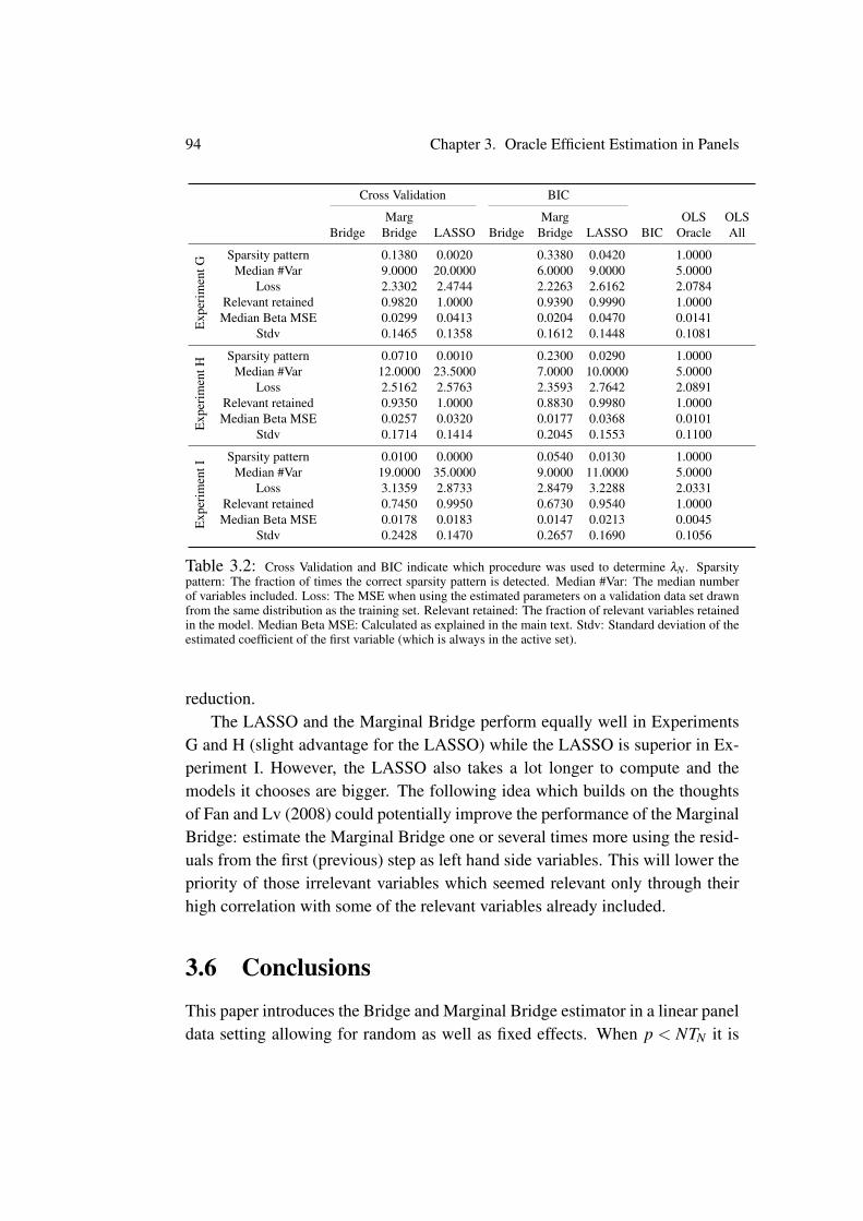
94 Chapter 3. Oracle Efficient Estimation in Panels
Cross Validation BIC
Marg Marg OLS OLSBridge Bridge LASSO Bridge Bridge LASSO BIC Oracle All
Exp
erim
entG
Sparsity pattern 0.1380 0.0020 0.3380 0.0420 1.0000Median #Var 9.0000 20.0000 6.0000 9.0000 5.0000
Loss 2.3302 2.4744 2.2263 2.6162 2.0784Relevant retained 0.9820 1.0000 0.9390 0.9990 1.0000Median Beta MSE 0.0299 0.0413 0.0204 0.0470 0.0141
Stdv 0.1465 0.1358 0.1612 0.1448 0.1081
Exp
erim
entH
Sparsity pattern 0.0710 0.0010 0.2300 0.0290 1.0000Median #Var 12.0000 23.5000 7.0000 10.0000 5.0000
Loss 2.5162 2.5763 2.3593 2.7642 2.0891Relevant retained 0.9350 1.0000 0.8830 0.9980 1.0000Median Beta MSE 0.0257 0.0320 0.0177 0.0368 0.0101
Stdv 0.1714 0.1414 0.2045 0.1553 0.1100
Exp
erim
entI
Sparsity pattern 0.0100 0.0000 0.0540 0.0130 1.0000Median #Var 19.0000 35.0000 9.0000 11.0000 5.0000
Loss 3.1359 2.8733 2.8479 3.2288 2.0331Relevant retained 0.7450 0.9950 0.6730 0.9540 1.0000Median Beta MSE 0.0178 0.0183 0.0147 0.0213 0.0045
Stdv 0.2428 0.1470 0.2657 0.1690 0.1056
Table 3.2: Cross Validation and BIC indicate which procedure was used to determine λN . Sparsitypattern: The fraction of times the correct sparsity pattern is detected. Median #Var: The median numberof variables included. Loss: The MSE when using the estimated parameters on a validation data set drawnfrom the same distribution as the training set. Relevant retained: The fraction of relevant variables retainedin the model. Median Beta MSE: Calculated as explained in the main text. Stdv: Standard deviation of theestimated coefficient of the first variable (which is always in the active set).
reduction.The LASSO and the Marginal Bridge perform equally well in Experiments
G and H (slight advantage for the LASSO) while the LASSO is superior in Ex-periment I. However, the LASSO also takes a lot longer to compute and themodels it chooses are bigger. The following idea which builds on the thoughtsof Fan and Lv (2008) could potentially improve the performance of the MarginalBridge: estimate the Marginal Bridge one or several times more using the resid-uals from the first (previous) step as left hand side variables. This will lower thepriority of those irrelevant variables which seemed relevant only through theirhigh correlation with some of the relevant variables already included.
3.6 Conclusions
This paper introduces the Bridge and Marginal Bridge estimator in a linear paneldata setting allowing for random as well as fixed effects. When p < NTN it is

3.6. Conclusions 95
shown that the Bridge estimator (and Marginal Bridge) has the oracle property.It sets all coefficients that are truly zero to zero and the asymptotic distributionof the estimator of the non zero coefficients is the same as if the sparsity patternhad been known. Monte Carlo experiments underscore this conclusion and areused to investigate the finite sample properties of the procedures. They alsoreveal that the Schwarz information criterion is more useful than 10-fold crossvalidation for selecting λN . This is encouraging since BIC is also faster thancross validation.
When p > NTN it is shown that the Marginal Bridge estimator still detectsthe correct sparsity pattern with probability converging to one. This is true inthe random as well as the fixed effects setting under a partial orthogonality as-sumption on the covariates. However, the Marginal Bridge works well evenwhen the relevant and irrelevant covariates are highly correlated. Furthermore,the Marginal Bridge estimates are extremely fast to compute since only marginalinformation is used to decide whether a variable is relevant or not. The MarginalBridge is also shown to perform well in the pN < NTN setting. In the pN > NTN
setting the Marginal Bridge does not always retain all relevant variables. An iter-ative procedure was proposed to solve this problem. Working out the propertiesof this procedure is left for future research.
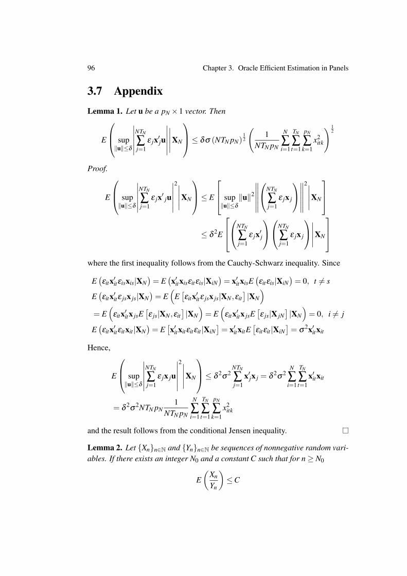
96 Chapter 3. Oracle Efficient Estimation in Panels
3.7 AppendixLemma 1. Let u be a pN×1 vector. Then
E
sup‖u‖≤δ
∣∣∣∣∣∣NTN
∑j=1
ε jx′ju
∣∣∣∣∣∣∣∣∣∣∣XN
≤ δσ (NTN pN)12
(1
NTN pN
N
∑i=1
TN
∑t=1
pN
∑k=1
x2itk
) 12
Proof.
E
sup‖u‖≤δ
∣∣∣∣∣∣NTN
∑j=1
ε jx′ ju
∣∣∣∣∣∣2∣∣∣∣∣XN
≤ E
sup‖u‖≤δ
‖u‖2
∥∥∥∥∥∥NTN
∑j=1
ε jx j
∥∥∥∥∥∥2∣∣∣∣∣XN
≤ δ
2E
NTN
∑j=1
ε jx′j
NTN
∑j=1
ε jx j
∣∣∣∣∣XN
where the first inequality follows from the Cauchy-Schwarz inequality. Since
E(εitx′itεisxis|XN
)= E
(x′itxisεitεis|XiN
)= x′itxisE
(εitεis|XiN
)= 0, t 6= s
E(εitx′itε jsx js|XN
)= E
(E[εitx′itε jsx js|XN ,εit
]|XN
)= E
(εitx′itx jsE
[ε js|XN ,εit
]|XN
)= E
(εitx′itx jsE
[ε js|X jN
]|XN
)= 0, i 6= j
E(εitx′itεitxit |XN
)= E
[x′itxitεitεit |XiN
]= x′itxitE
[εitεit |XiN
]= σ
2x′itxit
Hence,
E
sup‖u‖≤δ
∣∣∣∣∣∣NTN
∑j=1
ε jx ju
∣∣∣∣∣∣2∣∣∣∣∣XN
≤ δ2σ
2NTN
∑j=1
x′jx j = δ2σ
2N
∑i=1
TN
∑t=1
x′itxit
= δ2σ
2NTN pN1
NTN pN
N
∑i=1
TN
∑t=1
pN
∑k=1
x2itk
and the result follows from the conditional Jensen inequality.
Lemma 2. Let Xnn∈N and Ynn∈N be sequences of nonnegative random vari-ables. If there exists an integer N0 and a constant C such that for n≥ N0
E(
Xn
Yn
)≤C

3.7. Appendix 97
then
Xn ∈ Op(Yn)
Proof. It suffices to show that for any ε > 0 P(
XnYn
> Cε
)≤ ε for n ≥ N0.
Assume the opposite is true for some ε > 0 to reach a contradiction. Then,
E(
Xn
Yn
)=∫ Xn
YndP≥
∫Xn
Yn >Cε
Xn
YndP≥
∫Xn
Yn >Cε
Cε
dP≥ Cε
P
(Xn
Yn>
Cε
)> C
which is the desired contradiction.
Proof of Theorem 1. We first show that∥∥∥βN−β0
∥∥∥ ∈ Op
([pN+λNkNNTNρ1N
] 12
). Since
βN minimizes (3.6)
NTN
∑j=1
(y j−x′jβN
)2+λN
pN
∑k=1|βNk|γ ≤
NTN
∑j=1
(y j−x′jβ0
)2+λN
pN
∑k=1|β0k|γ
Defining ηN = λN ∑pNk=1 |β0k|γ this implies:
ηN ≥NTN
∑j=1
(y j−x′jβN
)2−
NTN
∑j=1
(y j−x′jβ0
)2
=NTN
∑j=1
([y j−x′jβN
]−[y j−x′jβ0
])([y j−x′jβN
]+[y j−x′jβ0
])
=NTN
∑j=1
[x′j(β0− βN)
]2+2
NTN
∑j=1
ε jx′j(
β0− βN
)Now define δN = (NTN)1/2Σ
1/2N (βN − β0), DN = (NTN)−1/2Σ
−1/2N X′N and
εN = (ε1, ...,εNTN )′. With these definitions
NTN
∑j=1
[x′j(β0− βN)
]2+2
NTN
∑j=1
ε jx′j(
β0− βN
)= δ
′NδN−2(DNεN)′δN
= ||δN−DNεN ||2−||DNεN ||2
which implies
||δN−DNεN ||2−||DNεN ||2−ηN ≤ 0

98 Chapter 3. Oracle Efficient Estimation in Panels
and by the sub additivity of x 7→ x1/2 yields ||δN−DNεN || ≤ ||DNεN ||+η1/2N . By
sub additivity of the norm ‖·‖ this implies ||δN || ≤ ||δN −DNεN ||+ ||DNεN || ≤2||DNεN ||+ η
1/2N . Since (x + y)2 ≤ 2x2 + 2y2 for x,y ∈ R by the convexity of
x 7→ x2 one has
||δN ||2 ≤ 4||DNεN ||2 +2ηN
Letting d j denote the j’th column of DN we may write DNεN = ∑NTNj=1 d jε j.
Using that DN is measurable with respect to XN , conclude
E(d′itεitdisεis
)= E
(d′itdisE
[εitεis|XN
])= E
(d′itdisE
[εitεis|XiN
])= 0, s 6= t
E(d′itεitd jsε js
)= E
(d′itεitd jsE
[ε js|XN ,εit
])= E
(d′itεitd js
[ε js|X jN
])= 0, i 6= j
E(d′itεitditεit
)= E
(d′itditE
[εitεit |XiN
])= E
(d′itdit
)= σ
2E(||dit ||2
)Hence,
E(‖DNεN‖2
)= E
∥∥∥∥∥∥
NTN
∑j=1
d jε j
∥∥∥∥∥∥2= E
NTN
∑j=1
d jε j
′NTN
∑j=1
d jε j
= σ2E
NTN
∑j=1
∥∥d j∥∥2
= σ2E(
tr(D′NDN
))= σ
2E(
tr(DND′N
))= σ
2tr(IpN
)= σ
2 pN
And so, E(||δN ||2
)≤ 4σ2 pN +2ηN . Hence,
(NTN)E((
βN−β0
)′ΣN
(βN−β0
))= E(δ ′NδN) = E(||δN ||2)≤ 4σ
2 pN +2ηN
Since the number of non zero coefficients is kN
ηN = λN
pN
∑k=1|β0 j|γ = λN
kN
∑k=1|β0 j|γ ≤ λNkNbγ
1
where the inequality is a consequence of assumption (A5). Since ρ1N is thesmallest eigenvalue of ΣN

3.7. Appendix 99
ρ1N ||βN−β0||2 = ρ1N
(βN−β0
)′(βN−β0
)≤(
βN−β0
)′ΣN
(βN−β0
)Hence,
E(
ρ1N ||βN−β0||2)≤ NTN
NTNE((
βN−β0
)′ΣN
(βN−β0
))≤ 4σ2 pN +2ηN
NTN≤
4σ2 pN +2λNkNbγ
1NTN
≤CpN +λNkNbγ
1NTN
for C = max(
4σ2,2bγ
1
). This implies
E
||βN−β0||2(pN+λNkNNTNρ1N
)≤C
By Lemma 2 this establishes ||βN −β0|| ∈ Op
([pN+λNkNNTNρ1N
] 12
). Next we show
that ||βN−β0|| ∈Op
(ρ−11N
(pN/(NTN)
)1/2)
. Like Huang et al. (2008) we use theidea from the proof of Theorem 3.2.5 in Van der Vaart and Wellner (1996). LetrN = ρ
−11N
(pN/(NTN)
)1/2. For every N partition the parameter space (excluding
β0) into the disjoint shells Sl,N =
β : 2l−1 <‖β −β0‖/rN ≤ 2l
where l ∈ Z.
If 2M <∥∥∥βN−β0
∥∥∥/rN for a given integer M then βN ∈⋃
l>M Sl,N . For the shell
which βN belongs to, the infimum of the map β 7→ LN(β )−LN(β0) is non posi-tive. Hence, for any δ > 0 11
11Note that∥∥∥βN−β0
∥∥∥/rN > 2M⊆⋃
l>M
inf
β∈Sl,N
(LN(β )−LN(β0)
)≤ 0
⊆
⋃l>M
inf
β∈Sl,N
(LN(β )−LN(β0)
)≤ 0
∩∥∥∥βN−β0
∥∥∥≤ δ
∪∥∥∥βN−β0
∥∥∥> δ
=
⋃l>M
inf
β∈Sl,N
(LN(β )−LN(β0)
)≤ 0
∩∥∥∥βN−β0
∥∥∥/rN ≤ δ/rN
∪∥∥∥βN−β0
∥∥∥> δ
⊆⋃l>M
2l−1<δ/rN
inf
β∈Sl,N
(LN(β )−LN(β0)
)≤ 0
∪∥∥∥βN−β0
∥∥∥> δ

100 Chapter 3. Oracle Efficient Estimation in Panels
P(∥∥∥βN−β0
∥∥∥/rN > 2M)
≤ ∑l>M
2l−1<δ/rN
P
(inf
β∈Sl,N
(LN(β )−LN(β0)
)≤ 0
)+P
(∥∥∥βN−β0
∥∥∥> δ
)(3.13)
The last term in (3.13) converges to 0 by the consistency of βN shown in thefirst part of the theorem. The theorem is established by proving that the first termon the right hand side can be made arbitrarily small by choosing M sufficientlylarge. To this is end let β ∈ Sl,N for an arbitrary l summed over, and notice that
LN(β )−LN(β0) =NTN
∑j=1
(y j−x′jβ
)2+λN
kN
∑k=1|β1k|γ +λN
mN
∑k=1|β2k|γ
−NTN
∑j=1
(y j−x′jβ0
)2−λN
kN
∑k=1|β01k|γ
≥NTN
∑j=1
(y j−x′jβ
)2+λN
kN
∑k=1|β1k|γ −
NTN
∑j=1
(y j−x′jβ0
)2−λN
kN
∑k=1|β01k|γ
=NTN
∑j=1
(x′j [β −β0]
)2−2
NTN
∑j=1
ε jx′j (β −β0)+λN
kN
∑k=1
(|β1k|γ −|β01k|γ
)(3.14)
Regarding the first term in (3.14),
NTN
∑j=1
(x′j [β −β0]
)2= [β −β0]
′NTN
∑j=1
x jx′j [β −β0] = NTN [β −β0]′ΣN [β −β0]
≥ NTN‖β −β0‖2ρ1N > NTN22(l−1)r2
Nρ1N
Regarding the third term in (3.14) we notice that β ∈ Sl,N and 2l−1 < δ/rN
implies that ‖β −β0‖/rN ≤ 2l < 2δ/rN . Hence, it suffices to consider β s satis-fying‖β −β0‖< 2δ . Since δ > 0 is arbitrary and the entries of β10 are boundeduniformly away from the 0 by b0 the mean value theorem may be applied toconclude that for some ζk between β1k and β10k
and conclude using the subadditivity of P.

3.7. Appendix 101
∣∣∣∣∣λN
kN
∑k=1
(|β1k|γ −|β01k|γ
)∣∣∣∣∣=∣∣∣∣∣λNγ
kN
∑k=1|ζk|γ−1sign(ζk)(β1k−β01k)
∣∣∣∣∣≤ cλN
kN
∑k=1|β1k−β01k| ≤ cλNk1/2
N ‖β −β0‖ ≤ cλNk1/2N 2lrN
where c = γ(b0 − 2δ )γ−1 and the second to last estimate follows fromJensen’s inequality. Hence, on Sl,N , λN ∑
kNk=1
(|β1k|γ −|β01k|γ
)≥−cλNk1/2
N 2lrN .Therefore, on Sl,N ,
LN(β )−LN(β0)≥−
∣∣∣∣∣∣2NTN
∑j=1
ε jx′j (β −β0)
∣∣∣∣∣∣+ρ1NNTN22(l−1)r2N− cλNk1/2
N 2lrN
Hence, by the conditional Markov inequality and Lemma 1
P
infβ∈Sl,N
(LN(β )−LN(β0)
)≤ 0
∣∣∣∣∣XN
≤ P
supβ∈Sl,N
∣∣∣∣∣∣2NTN
∑j=1
ε jx′j (β −β0)
∣∣∣∣∣∣≥ ρ1NNTN22(l−1)r2N− cλNk1/2
N 2lrN
∣∣∣∣∣XN
≤
E
supβ∈Sl,N
∣∣∣2∑NTNj=1 ε jx′j (β −β0)
∣∣∣∣∣∣∣∣XN
ρ1NNTN22(l−1)r2
N− cλNk1/2N 2lrN
≤σ(NTN pN)1/22lrN
(1
NTN pN∑
Ni=1 ∑
TNt=1 ∑
pNk=1 x2
itk
)1/2
ρ1NNTN22(l−1)r2N− cλNk1/2
N 2lrN
=2σ
(1
NTN pN∑
Ni=1 ∑
TNt=1 ∑
pNk=1 x2
itk
)1/2
2l−2− cλN(kN/(pNNTN)
)1/2
By assumption (A3) λN(kN/(pNNTN)
)1/2 → 0 and so 2l−2 −cλN
(kN/(NTN)
)1/2 ≥ 2l−3 for N sufficiently large. Hence, by iteratedexpectations and assumption (A1)

102 Chapter 3. Oracle Efficient Estimation in Panels
P
(inf
β∈Sl,N
(LN(β )−LN(β0)
)≤ 0
)≤ σ√
K2l−4
Finally, this implies that
∑l>M
2l−1<δ/rN
P
(inf
β∈Sl,N
(LN(β )−LN(β0)
)≤ 0
)≤ ∑
l>M
σ√
K2l−4
which is convergent and so the tail can be made arbitrarily small by choosingM sufficiently large.
Lemma 3. Suppose 0 < γ < 1. Let βN =(
β1N , β2N
). Then β2N = 0 with
probability converging to 1 under assumptions (A1)-(A7).
Proof. By Theorem 1 ||βN − β0|| ∈ Op (hN) with hN = ρ−11N (pN/(NTN))1/2 so
for all ε > 0 there exists a constant C such that for N sufficiently large
P(||βN−β0||/hN > C
)< ε ⇔ P
(||βN−β0|| ≤ChN
)≥ 1− ε
Put differently, βN ∈
β : ||β −β0|| ≤ChN
with probability converging to 1.Let β1N = β10 + hNu1 and β2N = β20 + hNu2 = hNu2. Choosing βN is thenequivalent to choosing u1 and u2. For u = (u′1,u
′2)′ one has ||u||= ||βN−β0||/hN
which is bounded by C with probability approaching 1. Hence, we may assume||u||2 = ||u1||2 + ||u2||2 ≤C2 and define
VN(u1,u2) = LN(β1N , β2N) = LN(β10 +hNu1,hNu2)
To establish the lemma it now suffices to show that for any u with ‖u‖ ≤

3.7. Appendix 103
C, VN(u1,u2)−VN(u1,0) > 0 with probability converging to 1 if u2 6= 0. Now,
VN(u1,u2)−VN(u1,0) =NTN
∑j=1
(y j−β
′01w j−hNu′1w j−hNu′2z j
)2 +λN
kN
∑k=1|β01k +hNu1k|γ
+λN
mN
∑k=1|hNu2k|γ −
NTN
∑j=1
(y j−β
′01w j−hNu′1w j
)2−λN
kN
∑k=1|β01k +hNu1k|γ
=NTN
∑j=1−hN(u′2z j)
[2(y j−β
′01w j−hNu′1w j)−hNu′2z j
]+λN
mN
∑k=1|hNu2k|γ
= h2N
NTN
∑j=1
(z′ju2)2 +2h2N
NTN
∑j=1
(w′ju1)(z′ju2)−2hN
NTN
∑j=1
(z′ju2)ε j +λNhγ
N
mN
∑k=1|u2 j|γ
Regarding the sum of the first two terms since 2xy≥−(x2 + y2)
h2N
NTN
∑j=1
(z′ju2)2 +2h2N
NTN
∑j=1
(w′ju1)(z′ju2)≥ h2N
NTN
∑j=1
(z′ju2)2−h2N
NTN
∑j=1
[(w′ju1)2 +(z′ju2)2
]=−h2
NNTNu′1Σ1Nu1 ≥−ρ−21N pNτ2C2
where the last inequality follows from assumption (A2) and the fact that ||u1|| ≤C. Hence,
h2N ∑
NTNj=1(z′iu2)2 +2h2
N ∑NTNj=1(w′iu1)(z′iu2)
pNρ−2N
≥−τ2C2
Regarding the third term it follows from Jensen’s inequality (conditional version)
E
∣∣∣∣∣∣NTN
∑j=1
(z′ju2)ε j
∣∣∣∣∣∣∣∣∣∣∣XN
≤E
NTN
∑j=1
(z′ju2)ε j
2∣∣∣∣∣XN
1/2
=
σ2
NTN
∑j=1
(z′ju2)2
1/2
= σ
NTN
∑j=1
u′2z jz′ju2
1/2
= σ(NTN)1/2 (u′2Σ2Nu2)1/2 ≤ σ(NTN)1/2
ρ1/22N C
where the last inequality used that
ρ2N = maxu∈RpN
u′ΣNuu′u
≥ maxu2∈RmN
(0′,u′2)ΣN(0′,u′2)′
(0′,u′2)(0′,u′2)′
= maxu2∈RmN
u′Σ2Nu2u′2u2

104 Chapter 3. Oracle Efficient Estimation in Panels
Hence, since hN is measurable wrt. σ(XN),
E
∣∣∣∣∣∣−2hN
NTN
∑j=1
(z′ju2)ε j
∣∣∣∣∣∣∣∣∣∣∣XN
≤ 2σhN(NTN)1/2ρ
1/22N C
and so
E
∣∣∣−2hN ∑
NTNj=1(z′ju2)ε j
∣∣∣hN(NTN)1/2ρ
1/22N
≤ 2σC
which by Lemma 2 shows that −2hN ∑NTNj=1(z′ju2)ε j is Op(hN(NTN)1/2ρ
1/22N ) =
Op(ρ−11N ρ
1/22N p1/2
N ). Hence,∣∣∣−2hN ∑NTNj=1(z′ju2)ε j
∣∣∣pNρ
−21N
∈ Op
ρ−11N ρ
1/22N p1/2
N
pNρ−21N
= Op
ρ1Nρ1/22N
p1/2N
⊆ Op(1)
by assumption (A7). Regarding the fourth term since u2 6= 0 we have
λNhγ
N/(pNρ−21N ) = λN
[ρ−11N (pN/NTN)1/2
]γ
/(pNρ−21N ) = λNρ
2−γ
1N (NTN)−γ/2 pγ/2−1N → ∞
by assumption (A4) and so the fourth term diverges to infinity. Since pNρ−21N ∈
Ωp(1) this completes the proof.
Proof of Theorem 2. The first part has been established in Lemma 3. Since βN
is consistent it follows from assumption (A5) that for an arbitrary ε > 0
P
(min
|β 1N j| |1≤ j ≤ k
+ ε < b0
)= P
k⋃j=1
|β1N j|+ ε < b0
= P
k⋃j=1
b0−|β1N j|> ε
≤ P
k⋃j=1
|β10 j|− |β1N j|> ε
≤ P
k⋃j=1
|β10 j− β1N j|> ε
≤ P(||β10− β1N j||> ε
)→ 0
Choosing ε = b0/2 shows that with probability converging to onemin
|β 1N j| |1≤ j ≤ k
≥ b0/2 and so β1N is bounded away from 0. Hence

3.7. Appendix 105
LN is differentiable at β1N with probability converging to one. And so β1N satis-fies
∂
∂β1LN(β1N , β2N) = 0
That is,
−2NTN
∑j=1
(y j−w′jβ1N− z′jβ2N
)w j +λNγψN = 0
with probability converging to 1 where ψN is a k×1 vector with l’th entry givenby ψNl = |β1Nl|γ−1sign(β1Nl). This can be rewritten as
−2NTN
∑j=1
(ε j−w′j(β1N−β10)− z′jβ2N
)w j +λNγψN = 0⇔
−2NTN
∑j=1
ε jw j +2NTN
∑j=1
w jw′j(β1N−β10)+2NTN
∑j=1
z′jβ2Nw j +λNγψN = 0⇔
Σ1N(β1N−β10) =1
NTN
NTN
∑j=1
ε jw j−λNγψN
2NTN− 1
NTN
NTN
∑j=1
z′jβ2Nw j
Hence, for any k×1 vector α
(NTN)1/2α′(β1N−β10) = (NTN)−1/2
NTN
∑j=1
α′Σ−11N ε jw j
−(1/2)γ(NTN)−1/2λNα
′Σ−11N ψN− (NTN)−1/2
NTN
∑j=1
α′Σ−11N z′jβ2Nw j
Since P(β2N = 0)→ 1 the last term equals 0 with probability converging to 1.From the Cauchy-Schwarz inequality in Rk it follows that
|α ′Σ−11N ψN | ≤ ||α ′Σ−1
1N ||||ψN ||
Since
||α ′Σ−11N ||
2 = α′Σ−11N Σ
−11N α = α
′Σ−21N α ≤ τ
−21N ||α||
2 ≤ τ−21 ||α||
2
by assumption (A2), we get with probability converging to one
|(1/2)(NTN)−1/2γλNα
′Σ−11N ψN | ≤ (1/2)(NTN)−1/2
γλNτ−11 ||α||||ψN ||
≤ (1/2)(NTN)−1/2γλNτ
−11 ||α||k
1/2(b0/2)(γ−1)
= (1/2)γτ−11 ||α||(b0/2)(γ−1)T−1/2
N N−1/2λNk1/2→ 0

106 Chapter 3. Oracle Efficient Estimation in Panels
by assumption (A3). Hence,
(NTN)1/2α′(β1N−β10) ∈ (NTN)−1/2
NTN
∑j=1
α′Σ−11N ε jw j +op(1)
Since s−1N = 1/
√σ2α ′Σ−1
1N α ≤ τ1/22 /(σ ||α||) by assumption (A2) it is also true
that
(NTN)1/2s−1N α
′(β1N−β10) ∈ (NTN)−1/2s−1N
NTN
∑j=1
α′Σ−11N ε jw j +op(1) (3.15)
Now, defining Wi,N = (wi1, ...,wiTN )′ and εi,N = (εi1, ...,εiNTN )′ one first noticesthat12
1NTN
NTN
∑j=1
w jw′j→ limN→∞
1NTN
NTN
∑j=1
E(
w jw′j)
= limN→∞
E(
1TN
W′1NW1N
)(3.16)
where the first limit is in probability. To see why (3.16) is true let Z j be a fixedentry in w jw′j, j = 1, ...,NTN . Letting η > 0 be arbitrary and using the Markovinequality
P
∣∣∣∣∣∣ 1NTN
NTN
∑j=1
Z j−1
NTN
NTN
∑j=1
E(Z j)∣∣∣∣∣∣> η
≤ E(
1NTN
∑NTNj=1
[Z j−E
(Z j)])2
η2
=E(
∑Ni=1 ∑
TNt=1[Zit−E (Zit)
])2
(NTNη)2 =∑
Ni=1 E
(∑
TNt=1[Zit−E (Zit)
])2
(NTNη)2
=N(
∑TNt=1Var(Z1t)+2∑
TNt=1 ∑
TNs>t Cov(Z1t , Z1s)
)(NTNη)2
≤N(TN max1≤t≤TN Var (Z1t)+2TN(TN−1)/2max1≤t≤TN Var (Z1t)
)(NTNη)2
=max1≤t≤TN Var (Z1t)
Nη2 → 0
12All limits are taken elementwise in the matrices.

3.7. Appendix 107
Hence,
(NTN)−1/2s−1N
NTN
∑j=1
α′Σ−11N ε jw j =
(NTN)−1/2∑
NTNj=1 α ′
(1
NTN∑
NTNj=1 w jw′j
)−1ε jw j√
σ2α ′(
1NTN
∑NTNj=1 w jw′j
)−1α
∈ N−1/2√σ2α ′
(E[
1TN
W′1NW1N
])−1
α
N
∑i=1
α′
(E[
1TN
W′1NW1N
])−1
T−1/2N W′iNεiN +op(1)
Now,
E
N
∑i=1
α′
(E[
1TN
W′1NW1N
])−1
T−1/2N W′iNεiN
= 0
by iterated expectations and
r2N : = E
N
∑i=1
α′
(E[
1TN
W′1NW1N
])−1
T−1/2N W′iNεiN
2
=N
∑i=1
E
α′
(E[
1TN
W′1NW1N
])−1
T−1/2N W′iNεiNε
′iNWiNT−1/2
N
(E[
1TN
W′1NW1N
])−1
α
= σ
2Nα′
(E[
1TN
W′1NW1N
])−1
α
Finally, let UiN = α ′(
E[
1TN
W′1NW1N
])−1
T−1/2N W′iNεiN . Since E(U2
iN) =
σ2α ′(
E[
1TN
W′1NW1N
])−1
α is convergent it is bounded. Furthermore,
α′E(
1TN
W′1NW1N
)α = E
(α′ 1NTN
W′NWNα
)∈[α′ατ1,α
′ατ2]
and so the eigenvalues of E[
1TN
W′1NW1N
]are also contained in [τ1,τ2]. This
implies r2N = σ2Nα ′
(E[
1TN
W′1NW1N
])−1
α ≥ σ2Nα ′α/τ2. Hence, the Lin-
deberg condition is satisfied since for all δ > 0

108 Chapter 3. Oracle Efficient Estimation in Panels
limN→∞
r−2N
N
∑i=1
∫|Ui,N|>δ rN
U2iNdP
≤ limN→∞
τ2
α ′ασ2
∫|U1N |>δ
√α ′ασ2
τ2
√N
U21NdP = 0
since for any ρ > 0 (let δ
√α ′ασ2
τ2= K)
limN→∞
P(
U21N1|U1N |>K
√N > ρ
)≤ lim
N→∞P(|U1N |> K
√N)≤ lim
N→∞
E(
U21N
)K2N
= 0
and
U21N
∞
N=1is uniformly integrable13. Hence,
N−1/2√σ2α ′
(E[
1TN
W′1NW1N
])−1
α
N
∑i=1
α′
(E[
1TN
W′1NW1N
])−1
T−1/2N W′iNεiN
d→ N(0,1)
And so by (3.15),
(NTN)1/2s−1N α
′(β1N−β10)d→ N(0,1)
or equivalently,
(NTN)1/2(β1N−β10)d→ N
0,σ2
(lim
N→∞E[
1TN
W′1NW1N
])−1 (3.17)
Proof of Theorem 3. (i) If TN = T for a fixed T , U1N = U1 for all N where U1 isdefined in the obvious way, does not depend on N and belongs to L2. Hence,
limK→∞
sup1≤N<∞
∫|U1N |>K
U21NdP = lim
K→∞
∫|U1|>K
U21 dP = 0
by Lebesgue’s Dominated Convergence Theorem.
13The uniform integrability of
U21N
∞
N=1implies that
U2
1N1|U1N |>K√
N∞
N=1is uniformly
integrable which is what is needed to utilize the well known fact that convergence in measureplus uniform integrability is equivalent to convergence in L1.
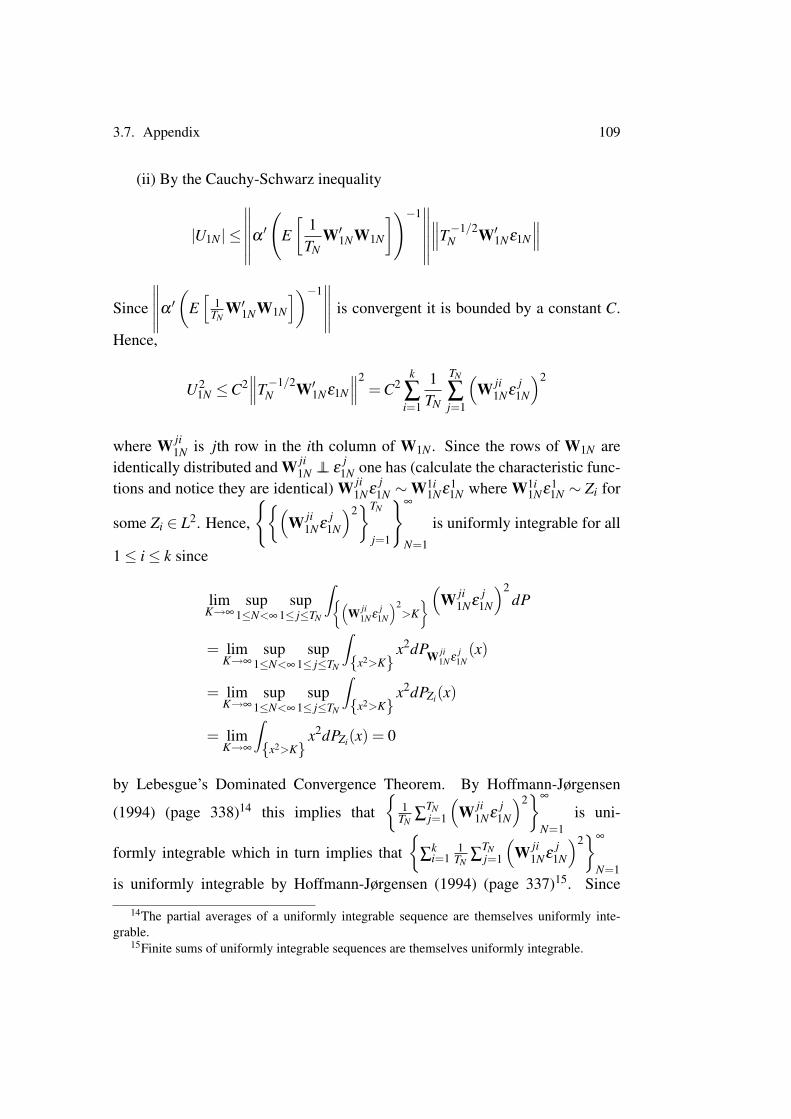
3.7. Appendix 109
(ii) By the Cauchy-Schwarz inequality
|U1N | ≤
∥∥∥∥∥∥α′
(E[
1TN
W′1NW1N
])−1∥∥∥∥∥∥∥∥∥T−1/2
N W′1Nε1N
∥∥∥Since
∥∥∥∥∥α ′(
E[
1TN
W′1NW1N
])−1∥∥∥∥∥ is convergent it is bounded by a constant C.
Hence,
U21N ≤C2
∥∥∥T−1/2N W′1Nε1N
∥∥∥2= C2
k
∑i=1
1TN
TN
∑j=1
(W ji
1Nεj
1N
)2
where W ji1N is jth row in the ith column of W1N . Since the rows of W1N are
identically distributed and W ji1N ⊥⊥ ε
j1N one has (calculate the characteristic func-
tions and notice they are identical) W ji1Nε
j1N ∼W1i
1Nε11N where W1i
1Nε11N ∼ Zi for
some Zi ∈ L2. Hence,
(W ji
1Nεj
1N
)2TN
j=1
∞
N=1
is uniformly integrable for all
1≤ i≤ k since
limK→∞
sup1≤N<∞
sup1≤ j≤TN
∫(W ji
1Nεj
1N
)2>K(W ji
1Nεj
1N
)2dP
= limK→∞
sup1≤N<∞
sup1≤ j≤TN
∫x2>K
x2dPW ji1Nε
j1N
(x)
= limK→∞
sup1≤N<∞
sup1≤ j≤TN
∫x2>K
x2dPZi(x)
= limK→∞
∫x2>K
x2dPZi(x) = 0
by Lebesgue’s Dominated Convergence Theorem. By Hoffmann-Jørgensen
(1994) (page 338)14 this implies that
1TN
∑TNj=1
(W ji
1Nεj
1N
)2∞
N=1is uni-
formly integrable which in turn implies that
∑ki=1
1TN
∑TNj=1
(W ji
1Nεj
1N
)2∞
N=1is uniformly integrable by Hoffmann-Jørgensen (1994) (page 337)15. Since
14The partial averages of a uniformly integrable sequence are themselves uniformly inte-grable.
15Finite sums of uniformly integrable sequences are themselves uniformly integrable.

110 Chapter 3. Oracle Efficient Estimation in Panels
C2
∑ki=1
1TN
∑TNj=1
(W ji
1Nεj
1N
)2∞
N=1dominates
U2
1N
this yields the desired
result.(iii) If W1N and ε1N are uniformly bounded U1N has moments of any order
and so
U21N
∞
N=1is uniformly integrable.
Proof of Corollary 1. For fixed TN (3.17) reads
N1/2(β1N−β10)d→ N
(0,σ2
(E[W′1W1
])−1)
where absence of subscript N indicates that the matrices no longer depend onTN . In the fixed effects setting W1 =
(DD′
)−1/2 DW1 and so
E(W′1W1
)= E
(W′
1D′(DD′
)−1/2 (DD′)−1/2 DW1
)= E
(W′1D′
(DD′
)−1 DW1
)= E
(¨W′1
¨W1
)where the last inequality used that D′
(DD′
)−1 D is symmetric and idempotentand that premultiplication of it corresponds to columnwise demeaning.
The proof of part (ii) is similar using W1 = Ω−1/2W1.
Next we turn to the properties of the Marginal Bridge estimator.
Lemma 4. For q even and any wN > 0,
P
wN > max1≤k≤m
∣∣∣∣∣∣NT
∑j=1
x jkε j
∣∣∣∣∣∣≥ 1− Km(NTN)q/2
wqN
Proof. By the Markov inequality,
P
wN > max1≤k≤m
∣∣∣∣∣∣NT
∑j=1
x jkε j
∣∣∣∣∣∣= 1−P
max1≤k≤m
∣∣∣∣∣∣NTN
∑j=1
x jkε j
∣∣∣∣∣∣≥ wN
≥ 1−E(
max1≤k≤m
∣∣∣∑NTNj=1 x jkε j
∣∣∣q)wq
N
Since for any sequence of random variables Zkmk=1 ⊆ Lq
E(
max1≤k≤m
Zqk
)≤ E
(m
∑k=1
Zqk
)≤ m max
1≤k≤mE(Zq
k
)

3.7. Appendix 111
it suffices to show that E(
∑NTNj=1 x jkε j
)q≤ K(NTN)q/2 for all k ∈ 1, ...,m. By
the multinomial theorem
E
NTN
∑j=1
x jkε j
q
= E
∑|α|=q
(qα
)NTN
∏j=1
(x jkε j)α j
where we have used the multi-index convention α = (α1, ...,αNT ) and |α| = qmeans ∑
NTNj=1 α j = q. The sum is taken over all such vectors α whose en-
tries add up to q. Since (XiN ,εiN) is i.i.d. and XiN ⊥⊥ εiN it follows that(X1N ,ε1N , ...,XNN ,εNN) are independent (calculate the characteristic functionand observe that it factorizes). This implies XN ⊥⊥ εN . Finally, it is seen thatε11, ...,εNTN are independent and (again calculate the characteristic function andobserve that it factorizes by using (XiN ,εiN) is i.i.d and the that uncorrelated-ness implies independence for gaussian variables.). From these observations itfollows that all summands including an α j = 1 for some j = 1, ...,NTN equal0 since E(ε j) = 0 for all j = 1, ...,NTN . It remains to be shown that no other
term is of greater order than O((NTN)q/2
). So assume min1≤ j≤NTN α j ≥ 2 16.
Consider the set A of all vectors α with s entries different from 0 and larger thanor equal to 2 with non-zero values a1, ...,as and a1 + ...+as = q.
16Here we follow the convention of setting t0 = 1 even when t = 0 and so we only have toconsider the case min1≤ j≤NTN α j ≥ 2.

112 Chapter 3. Oracle Efficient Estimation in Panels
E
∑α∈A
NTN
∏j=1
(x jkε j)α j
= E
NTN
∑j1=1
NTN
∑j2 6= j1
...NTN
∑js /∈ j1,..., js−1
(x j1kε j1)a1(x j2kε j2)
a2 · ... · (x jskε js)as
= KE
NTN
∑j1=1
NTN
∑j2 6= j1
...NTN
∑js /∈ j1,..., js−1
(x j1k)a1(x j2k)a2 · ... · (x jsk)as
≤ K(NTN)q/2E
NTN
∑j1=1
NTN
∑j2 6= j1
...NTN
∑js /∈ j1,..., js−1
[x2
j1k
NTN
]a1/2[x2
j2k
NTN
]a2/2
· ... ·
[x2
jsk
NTN
]as/2
= K(NTN)q/2E
NTN
∑j1=1
[x2
j1k
NTN
]a1/2 NTN
∑j2 6= j1
[x2
j2k
NTN
]a2/2
· ... ·NTN
∑js /∈ j1,..., js−1
[x2
jsk
NTN
]as/2
≤ K(NTN)q/2
where the second equality used XN ⊥⊥ εN and K := E(εa11 ) · ... ·E(εas
1 ). The firstestimate follows from the nonnegativity of all terms on the right hand side. The
last estimate uses that for any subset S of 1, ...,NTN, ∑ j∈S
[x2
jk/(NTN)]ai/2
≤
∑NTNj=1
[x2
jk/(NTN)]ai/2
≤ ∑NTNj=1
[x2
jk/(NTN)]
= 1 since[x2
jk/(NTN)]≤ 1 and so[
x2jk/(NTN)
]ai/2≤[x2
jk/(NTN)]
for ai ≥ 2. Since s was arbitrary and there areonly finitely many terms of the above kind this establishes the lemma.
Proof of Theorem 4. Let εN = (ε1, ...,εNTN )′ and recall ξNk =

3.7. Appendix 113
1/(NTN)∑NTNj=1 w′jβ10x jk. Then,
UN(β ) =pN
∑k=1
NTN
∑j=1
(y j− x jkβk
)2 +λN
pN
∑k=1|βk|γ
=pN
∑k=1
NTN
∑j=1
y2j +NTNβ
2k −2
NTN
∑j=1
y jx jkβk
+λN
pN
∑k=1|βk|γ
=pN
∑k=1
NTN
∑j=1
ε2j +
NTN
∑j=1
(w′jβ01)2 +2NTN
∑j=1
(w′jβ01)ε j +NTNβ2k −2
NTN
∑j=1
(ε j +w′jβ01)x jkβk
+λN
pN
∑k=1|βk|γ
=pN
∑k=1
NTN
∑j=1
ε2j +
NTN
∑j=1
(w′jβ01)2 +2NTN
∑j=1
(w′jβ01)ε j +NTNβ2k −2(ε ′Nxk +NTNξNk)βk
+λN
pN
∑k=1|βk|γ
So minimizing UN(β ) is equivalent to minimizing
∑pNk=1
[NTNβ 2
k −2(ε ′Nxk +NTNξNk)βk +λN |βk|γ]. Since 0 < γ < 1 it fol-
lows from Lemma A of Knight and Fu (2000) that βk = 0 if and only if
λN/(NTN) > |ε ′Nxk/(NTN)+ξNk|2−γcγ
where cγ =(
22−γ
)(2(2−γ)
2−γ
)1−γ
. Defining wN = c−1/(2−γ)γ (λN/(NTN)γ/2)1/(2−γ)
the above inequality is equivalent to
wN > (NTN)−1/2|ε ′Nxk +(NTN)ξNk|
So to prove the theorem it is enough to show
P(
wN > (NTN)−1/2 maxk∈JN
∣∣ε ′Nxk +(NTN)ξNk∣∣)→ 1 (3.18)
and
P(
wN > (NTN)−1/2 mink∈KN
∣∣ε ′Nxk +(NTN)ξNk∣∣)→ 0 (3.19)

114 Chapter 3. Oracle Efficient Estimation in Panels
We first prove (3.18). On AN =
∣∣∣∑NTNj=1 x jkx jl
∣∣∣(NTN)1/2 ≤ c0, k ∈ KN , l ∈ JN
and under
assumption (B6)
maxl∈JN
(NTN)1/2∣∣ξNl∣∣= max
l∈JN
1(NTN)1/2
∣∣∣∣∣∣NTN
∑j=1
kN
∑k=1
x jkβ10kx jl
∣∣∣∣∣∣= max
l∈JN
1(NTN)1/2
∣∣∣∣∣∣kN
∑k=1
β10k
NTN
∑j=1
x jkx jl
∣∣∣∣∣∣≤maxl∈JN
kN
∑k=1|β10k|
∣∣∣∣∣∣ 1(NTN)1/2
NTN
∑j=1
x jkx jl
∣∣∣∣∣∣≤ b1c0kN
Hence,
P(
wN > (NTN)−1/2 maxk∈JN|ε ′Nxk +(NTN)ξNk|
)≥ P
(wN > (NTN)−1/2 max
k∈JN|ε ′Nxk|+(NTN)1/2 max
k∈JN|ξNk|, AN
)≥ P
(wN > (NTN)−1/2 max
k∈JN|ε ′Nxk|+b1c0kN , AN
)≥ P
(wN > (NTN)−1/2 max
k∈JN|ε ′Nxk|+b1c0kN
)+P(AN)−1
where the last estimate follows from the inclusion-exclusion principle. ByLemma 4 for every even q,
P(
(NTN)1/2 (wN−b1c0kN) > maxk∈JN|ε ′Nxk|
)≥ 1− KmN(NTN)q/2(
(NTN)1/2[wN−b1c0kN ])q
= 1−KmN/wq
N(1−b1c0kN/wN
)q
Furthermore, by assumption (B4) we may choose q sufficiently large such that
mN/wqN ∈ O(1)
mN(λN(NTN)−γ/2
)q/(2−γ) → 0
and by assumption (B3)
b1c0kN/wN ∈ O(1)kN(
λN(NTN)−γ/2)1/(2−γ) → 0

3.7. Appendix 115
Finally, P(AN) can be made arbitrarily close to 1 by assumption (B5) whichestablishes (3.18). Next we verify (3.19).
P(
wN > (NTN)−1/2 mink∈KN|ε ′Nxk +(NTN)ξNk|
)
= P
⋃k∈KN
wN > |(NTN)−1/2
ε′Nxk +(NTN)1/2
ξNk|
≤ ∑k∈KN
P(
wN > |(NTN)−1/2ε′Nxk +(NTN)1/2
ξNk|)
(3.20)
Since mink∈KN |ξNk| ≥ ξ0 > 0 by assumption (B1) we may write,
P(
wN > |(NTN)−1/2ε′Nxk +(NTN)1/2
ξNk|)
≤ P(
wN > (NTN)1/2|ξNk|− (NTN)−1/2|ε ′Nxk|)
≤ P(
wN > (NTN)1/2ξ0− (NTN)−1/2|ε ′Nxk|
)= P
((NTN)−1/2|ε ′Nxk|> (NTN)1/2
ξ0−wN
)= 1−P
((NTN)1/2
ξ0−wN ≥ (NTN)−1/2|ε ′Nxk|)
≤ 1−P(
(NTN)1/2ξ0−wN > (NTN)−1/2|ε ′Nxk|
)By Lemma 4,
P
((NTN)1/2
((NTN)1/2
ξ0−wN
)> |ε ′Nxk|
)≥1− K(NTN)q/2(
(NTN)1/2[(NTN)1/2ξ0−wN ])q
(3.21)
= 1− K((NTN)1/2ξ0−wN)q
(3.22)
And so for all k ∈ KN
P(
wN > |(NTN)−1/2ε′Nxk +(NTN)1/2
ξNk|)≤ K
((NTN)1/2ξ0−wN)q

116 Chapter 3. Oracle Efficient Estimation in Panels
Inserting this into (3.20) yields
P(
wN > (NTN)−1/2 mink∈kN|ε ′Nxk +(NTN)ξNk|
)≤ KkN
((NTN)1/2ξ0−wN)q
=KkN/(NTN)q/2(
ξ0−wN/(NTN)1/2)q
By assumption (B2),
wN
(NTN)1/2 ∈ O(1)
(λN(NTN)−γ/2
(NTN)(2−γ)/2
)1/(2−γ)
= O(1)(λN/(NTN)
)1/(2−γ) ⊆ o(1)
Furthermore, for any q≥ 1, kN/(NTN)q/2→ 0 by (B3). Hence,
P(
wN > (NTN)−1/2 mink∈KN|ε ′Nxk +(NTN)ξNk|
)→ 0.
3.8 Bibliography
Arellano, M. (2003). Panel data econometrics. Oxford University Press, Oxford.
Candes, E. and T. Tao (2007). The Dantzig selector: statistical estimation whenp is much larger than n. Annals of Statistics 35, 2313–2351.
Fan, J. and J. Lv (2008). Sure independence screening for ultrahigh dimensionalfeature space. Journal of the Royal Statistical Society: Series B (StatisticalMethodology) 70, 849–911.
Friedman, J., T. Hastie, H. Hofling, and R. Tibshirani (2007). Pathwise coordi-nate optimization. The Annals of Applied Statistics 1(2), 302–332.
Hoffmann-Jørgensen, J. (1994). Probability with a View Toward Statistics, Vol-ume 1. Chapman and Hall Probability Series, New-York: Chapman & Hall.
Huang, J., J. Horowitz, and S. Ma (2008). Asymptotic properties of bridge esti-mators in sparse high-dimensional regression models. Annals of Statistics 36,587–613.

3.8. Bibliography 117
Hunter, D. and R. Li (2005). Variable selection using MM algorithms. Annalsof Statistics 33, 1617.
Knight, K. and W. Fu (2000). Asymptotics for lasso-type estimators. Annals ofStatistics 28, 1356–1378.
Meinshausen, N. and B. Yu (2009). Lasso-type recovery of sparse representa-tions for high-dimensional data. Annals of Statistics 37, 246–270.
Stoyanov, J. (1997). Counterexamples in probability (2 ed.). Chichester-NewYork.
Tibshirani, R. (1996). Regression shrinkage and selection via the lasso. Journalof the Royal Statistical Society. Series B (Methodological) 58, 267–288.
Van der Vaart, A. and J. Wellner (1996). Weak convergence and empirical pro-cesses. Springer Verlag, New York.
Zou, H. (2006). The adaptive lasso and its oracle properties. Journal of theAmerican Statistical Association 101, 1418–1429.

SCHOOL OF ECONOMICS AND MANAGEMENT AARHUS UNIVERSITY – BARTHOLINS ALLÉ 10 – BUILDING 1322
DK-8000 AARHUS C – TEL. +45 8942 1111 - www.econ.au.dk
PhD Theses:
1999-4 Philipp J.H. Schröder, Aspects of Transition in Central and Eastern Europe.
1999-5 Robert Rene Dogonowski, Aspects of Classical and Contemporary European Fiscal
Policy Issues.
1999-6 Peter Raahauge, Dynamic Programming in Computational Economics.
1999-7 Torben Dall Schmidt, Social Insurance, Incentives and Economic Integration.
1999 Jørgen Vig Pedersen, An Asset-Based Explanation of Strategic Advantage.
1999 Bjarke Jensen, Five Essays on Contingent Claim Valuation.
1999 Ken Lamdahl Bechmann, Five Essays on Convertible Bonds and Capital Structure
Theory.
1999 Birgitte Holt Andersen, Structural Analysis of the Earth Observation Industry.
2000-1 Jakob Roland Munch, Economic Integration and Industrial Location in Unionized
Countries.
2000-2 Christian Møller Dahl, Essays on Nonlinear Econometric Time Series Modelling.
2000-3 Mette C. Deding, Aspects of Income Distributions in a Labour Market Perspective.
2000-4 Michael Jansson, Testing the Null Hypothesis of Cointegration.
2000-5 Svend Jespersen, Aspects of Economic Growth and the Distribution of Wealth.
2001-1 Michael Svarer, Application of Search Models.
2001-2 Morten Berg Jensen, Financial Models for Stocks, Interest Rates, and Options: Theory
and Estimation.
2001-3 Niels C. Beier, Propagation of Nominal Shocks in Open Economies.
2001-4 Mette Verner, Causes and Consequences of Interrruptions in the Labour Market.
2001-5 Tobias Nybo Rasmussen, Dynamic Computable General Equilibrium Models: Essays
on Environmental Regulation and Economic Growth.

2001-6 Søren Vester Sørensen, Three Essays on the Propagation of Monetary Shocks in Open
Economies.
2001-7 Rasmus Højbjerg Jacobsen, Essays on Endogenous Policies under Labor Union
Influence and their Implications.
2001-8 Peter Ejler Storgaard, Price Rigidity in Closed and Open Economies: Causes and
Effects.
2001 Charlotte Strunk-Hansen, Studies in Financial Econometrics.
2002-1 Mette Rose Skaksen, Multinational Enterprises: Interactions with the Labor Market.
2002-2 Nikolaj Malchow-Møller, Dynamic Behaviour and Agricultural Households in
Nicaragua.
2002-3 Boriss Siliverstovs, Multicointegration, Nonlinearity, and Forecasting.
2002-4 Søren Tang Sørensen, Aspects of Sequential Auctions and Industrial Agglomeration.
2002-5 Peter Myhre Lildholdt, Essays on Seasonality, Long Memory, and Volatility.
2002-6 Sean Hove, Three Essays on Mobility and Income Distribution Dynamics.
2002 Hanne Kargaard Thomsen, The Learning organization from a management point of
view - Theoretical perspectives and empirical findings in four Danish service
organizations.
2002 Johannes Liebach Lüneborg, Technology Acquisition, Structure, and Performance in
The Nordic Banking Industry.
2003-1 Carter Bloch, Aspects of Economic Policy in Emerging Markets.
2003-2 Morten Ørregaard Nielsen, Multivariate Fractional Integration and Cointegration.
2003 Michael Knie-Andersen, Customer Relationship Management in the Financial Sector.
2004-1 Lars Stentoft, Least Squares Monte-Carlo and GARCH Methods for American
Options.
2004-2 Brian Krogh Graversen, Employment Effects of Active Labour Market Programmes:
Do the Programmes Help Welfare Benefit Recipients to Find Jobs?
2004-3 Dmitri Koulikov, Long Memory Models for Volatility and High Frequency Financial
Data Econometrics.
2004-4 René Kirkegaard, Essays on Auction Theory.

2004-5 Christian Kjær, Essays on Bargaining and the Formation of Coalitions.
2005-1 Julia Chiriaeva, Credibility of Fixed Exchange Rate Arrangements.
2005-2 Morten Spange, Fiscal Stabilization Policies and Labour Market Rigidities.
2005-3 Bjarne Brendstrup, Essays on the Empirical Analysis of Auctions.
2005-4 Lars Skipper, Essays on Estimation of Causal Relationships in the Danish Labour
Market.
2005-5 Ott Toomet, Marginalisation and Discouragement: Regional Aspects and the Impact
of Benefits.
2005-6 Marianne Simonsen, Essays on Motherhood and Female Labour Supply.
2005 Hesham Morten Gabr, Strategic Groups: The Ghosts of Yesterday when it comes to
Understanding Firm Performance within Industries?
2005 Malene Shin-Jensen, Essays on Term Structure Models, Interest Rate Derivatives and
Credit Risk.
2006-1 Peter Sandholt Jensen, Essays on Growth Empirics and Economic Development.
2006-2 Allan Sørensen, Economic Integration, Ageing and Labour Market Outcomes
2006-3 Philipp Festerling, Essays on Competition Policy
2006-4 Carina Sponholtz, Essays on Empirical Corporate Finance
2006-5 Claus Thrane-Jensen, Capital Forms and the Entrepreneur – A contingency approach
on new venture creation
2006-6 Thomas Busch, Econometric Modeling of Volatility and Price Behavior in Asset and
Derivative Markets
2007-1 Jesper Bagger, Essays on Earnings Dynamics and Job Mobility
2007-2 Niels Stender, Essays on Marketing Engineering
2007-3 Mads Peter Pilkjær Harmsen, Three Essays in Behavioral and Experimental
Economics
2007-4 Juanna Schrøter Joensen, Determinants and Consequences of Human Capital
Investments
2007-5 Peter Tind Larsen, Essays on Capital Structure and Credit Risk

2008-1 Toke Lilhauge Hjortshøj, Essays on Empirical Corporate Finance – Managerial
Incentives, Information Disclosure, and Bond Covenants
2008-2 Jie Zhu, Essays on Econometric Analysis of Price and Volatility Behavior in Asset
Markets
2008-3 David Glavind Skovmand, Libor Market Models - Theory and Applications
2008-4 Martin Seneca, Aspects of Household Heterogeneity in New Keynesian Economics
2008-5 Agne Lauzadyte, Active Labour Market Policies and Labour Market Transitions in
Denmark: an Analysis of Event History Data
2009-1 Christian Dahl Winther, Strategic timing of product introduction under heterogeneous
demand
2009-2 Martin Møller Andreasen, DSGE Models and Term Structure Models with
Macroeconomic Variables
2009-3 Frank Steen Nielsen, On the estimation of fractionally integrated processes
2009-4 Maria Knoth Humlum, Essays on Human Capital Accumulation and Educational
Choices
2009-5 Yu Wang, Economic Analysis of Open Source Software
2009-6 Benjamin W. Blunck, Creating and Appropriating Value from Mergers and
Acquisitions – A Merger Wave Perspective
2009-7 Rune Mølgaard, Essays on Dynamic Asset Allocation and Electricity Derivatives
2009-8 Jens Iversen, Financial Integration and Real Exchange Rates: Essays in International
Macroeconomics
2009-9 Torben Sørensen, Essays on Human Capital and the Labour Market
2009-10 Jonas Staghøj, Essays on Unemployment and Active Labour Market Policies
2009-11 Rune Majlund Vejlin, Essays in Labor Economics
2009-12 Nisar Ahmad, Three Essays on Empirical Labour Economics
2010-1 Jesper Rosenberg Hansen, Essays on Application of Management Theory in Public
Organizations - Changes due to New Public Management
2010-2 Torben Beedholm Rasmussen, Essays on Dynamic Interest Rate Models and Tests for
Jumps in Asset Prices

2010-3 Anders Ryom Villadsen, Sources of Organizational Similarity and Divergence: Essays
on Decision Making and Change in Danish Municipalities Using Organizational
Institutionalism
2010-4 Eske Stig Hansen, Essays in Electricity Market Modeling
2010-5 Marías Halldór Gestsson, Essays on Macroeconomics and Economic Policy
2010-6 Niels Skipper, Essays on the Demand for Prescription Drugs
2010-7 Thomas Quistgaard Pedersen, Return predictability and dynamic asset allocation
2011-1 Malene Kallestrup Lamb, Health, Retirement and Mortality
2011-2 Lene Kromann, Essays on Productivity and Labour Supply
2011-3 Firew Bekele Woldeyes, Essays on Government Budgets in Developing Countries
2011-4 Anders Bredahl Kock, Forecasting and Oracle Efficient Econometrics