Government agencies the world over have been pursu- mg an ‘active’ manpoacr polic>. attempting to In- Rucnce the supply of and demand for manposer m various private and public sectors and mdustrles. The recent energy crisis in the United States has lead to the reevaluation of the role of coal in the energy picture. and a5 a consequence officials have become interested in the prospects for adequate labor suppI! in the coal industry.

A brlet history will put the problem in perspective. Aggregate emplo) ment III hltummous coal mining de- clined by 16.5 per cent from 169.400 men in 1960 to 124.533 III 1969 During this time period, coal produc- tion increased hk 31.Y per cent from 4 15.5 m1111on tons III 1960 to 560 5 mllllon tons m 19hY. Employment rose m lY70 to 140.1-W men and further mcrcascd m 1971 to 145.661. Increased employment IS due to a comhma- tlon of ( 1) sharp Increases in coal production and (2) decreases m productlvlty attributed mainly to the Health and Safety Act of 1969

C‘oal production in the year 1000 might bc as great as.3000 m&on tons to meet the ever expandmg energy demand\ of the US. Although the short term expert- ence does not suggest labor shortages. a combmation of factors suggests long term shortages might occur: ( 1) age structure of the coal work force: (2) social status of underground miners: (3) constramts of the Health and Safety Act: and. (3) uncertainty arismg out of past history of hiring mainly to replace workors deceased or retired.

The economist’s typical reaction to such B dilemma is that it all depends on the wages the coal industry is willing to pay miners. However, wage rates are limited by productivity. conventlon. and m recent years h) law. Moreover, It has hecn asserted that the wage elas- ticity (ix. the sensitivity of supply to changes m the wage rate) of coal miners (especially underground) IS rather low. mdlcatmg that even substantial wage hikes may not induce sufficient labor supply to meet expected demand.

It IS assumed m this paper that the present state of

* The stud) L%US aupportcd by the Bureau of Mmes. U S. Department of the lntcrlor Vlehs uxprrsscd m this paper do not necessarily reflect the official posltlon of the Bureau of M mrs

affaalrs in the bituminous coal mining industry concern- ing wages, fringe benefits. working conditions, inJury and filtahty rates. union influences, and locational fac- tors. relative to conditions in other industries employ- mg workers with similar characteristics, will remain stable during the forecastmg period. Moreover. the paper will concentrate on the supply side of the equa- tion. providing demand forecasts only in a summary form at the end of the paper. This is necessitated by the complexity of the demand and supply forecasting methodologies [I. 21.

The analysis of labor supply consists of two parts: (I) procedures to estimate the expected labor force of coal miners for each of the prediction years. disregard- ing new entrants to the mining labor force; and (7) estl- matlon of the expected number of entrants into the mining labor force, by age. In addition, an assessment of the prohahihty of manpower shortages m each of the forecast years will he made on the basis of the best available manpower demand estimates.

(A) PROCEDLRES TO ESTIMATE EXPECTED LABOR FORCE OF RITI’MINOUS COAL MINERS. DISREGARDING

Two methods are discussed here that may be utilized to estimate the number of coal miners employed in a given base year---say 197Gwho will remain in the mmmg workforce m given target years-say 1975, 19X5. and 7000. The first method employs Fullerton’s estimates of separation rates for men. due to all causes C-i]. The second method employs the concept of expected working life.

Rlctl& 1. Let I!,,., denote the number of miners of age s employed in year t. Let S, denote the expected rate of separation due to all causes for male workers ofage s. S, indicates the probability that an individual of age .k will leave the labor force between age Y and \’ + I due to either death or retirement (retirement may he due to dlsablhty, inability to find suitable employment. old age. or other reasons). The present analysis assumes that indlvlduals who are m the min- ing industry at year r will remam there until death or retncment. Moreover. it IS assumed that the prob- ability of death or retirement for a miner 1s identical

194 ELCHAFSAU COHK, JON P. NELW~ and GEORGE R. NEUMANN

Table 1 Estrmated drstrrbution of bttummous coal mmers by age, United States. 1970

Age 15-19 20-24 25-29 30-33 35-39 40-44 35-49 j&54 55-59 6G-64 65-69 Total

I Number m UMW sample 1099 8312 10516 9792 9197 12,294 13.715 15.113 12.319 5551 803 99.62 I 2. Proportion in UMW sample ()()I 1 0.083 0.106 0 IVX! 0.092 0.173 0.138 0.152 0.123 0.056 0 008 I no0 3. Estrmated number m labor

force. hnr (2) Y 130. 141 1547 11.632 14.855 13.734 12,893 17.237 70.171 71,301 17.237 784X 11’1 I 10.14 1

Sources Line I from Beneficiarres Ehgrble for Hosprtal and Medrcal Care. Part C. Table I I Unrted Mme Workers of America Welfarc and Retnement Fund, Washmgton, D C (September 1970).

Total of Lme 3 from Umted States Bureau of Mmes. ~\fnwuls Yeurhoo~. 1970 Edn.

to that of other males in the United States labor force.* The number of miners who were of age s in 1970

expected to remain in the labor force in the year T.

~(L,,,,“l, is calculated from the following equation: I lu-0~1

UL \.,97& = L,,,,,,, T1 (1 - S,+J (1) j L 0

where I - S, is the labor force retention rate between age x and .Y -t 1, and Tis the forecast year. The total number of mmers that are expected to remain in the labor force by the year T is therefore given by the fol- lowing equation:

The limits on the summation sign indicate only that we sum over all relevant ages. In practice, the age range may be limited to 17-70. Moreover, since the data are typically given in age brackets. such as 17-19. 7G-24. etc., the calculations of the expected number of miners may be based upon 5-yr intervals for the relevant age groupings.

It should be noted that data on the age distribution of miners are available only for a sample of the total mining population. Here it will be assumed that the age distribution of all miners is identical to that which is found in the sample. The calculation is then straight- forward. If L: is the number of active miners of age .Y in the sample, then the proportion. pXT of miners of age x m the sample is given by:

* In its recent report. the Appalachran Regional Commrs- ston [4] took exception to thus assumptton. To drstmgursh the mmmg populatron from the general workforce, the Commiwon utrhzed a measure It terms “the probability of noncontractron of the Black Lung disease ” The mam drau- back of the approach wrth regard to its utrltzatron m thus study 1s the lack of distmctron between surface and under- ground miners. Also, It IS qune possible that full ample- mentatron of the Federal Coal Health and Safety Act of 1969 would consrderably reduce the probabrlity of contrac- tron of Black Lung drsease among mmers.

Assummg that the p, values apply to the entire mm- mg workforce. the number of miners in each age bracket IS given by:

L, = pX (total employment in mining). (41

nfrtlzotf 2. The prmcipal drawback of Method 1 is its reliance on data for the entire male workforce of the United States. It is probable that rates of separation m the mmmg Industry, especially for the 55.-65 age bracket, are different from those that are found for the entire male population. It would therefore be desirable to estimate labor availability on the basis of data per- taming to miners alone.

Given data on the number of miners in each age group. it is possible to make use of the general metho- dology developed to estimate expected workhfe [3]. Using the terminology discussed in the previous sec- tion, the expected remaining worklife (in years) for a miner of age I, denoted by evv,, may be derived from the followmg formula:

a(‘, =

i 1 i L, \L,. (5) , = 1

Again. the formula will be modified to some extent to take account of the fact that data on L, are available only in age brackets.

Once t+v, has been calculated for each age bracket, it is possible to determine whether mdividuals m a par- ticular age group are likely to remain in the workforcc by a given target date. For example, if the remaming workhfe for miners aged 15 19 is at least 40 yr then it is quite obvious that miners of this age m 1970 will form part of the workforce up to the year 2010. assum- ing no inter-industry mobility of any kind nor new entries mto the mining workforce

Mrthod 1. The United Mine Workers of America (UMWA) Welfare and Retirement Fund maintams sta- tistics of the number of active miners. hi, qe. eligible to receive hospital and medical benefits from the un- ion In 1970. there were 99.621 active miners in that category. In all, the I-J.S. Bureau of Mines reports that there were 140,141 miners in 1970. The UMWA age- distribution data are apparently the most comprehen- sive available. If it is assumed that the age distribution

Forecasting aggregate supply of coal mmers 795

Tahlc 2 Rates of sepurstlon from the labor force. Umted States. M&x I Y6X

Age (1)

16 19 20 24 25-79 3&3J 35-39 -K--&l 45-49 5(&5J 55-57 6%64 65-69

Rate of srpxatlon (S,) (due to all Caubes)

00017 0.0022 0 00’0 0.0025 0 004.l 0 OO65 OOIO9 0OlX-I 0.0337 0 09-l I 0 1763

I - s,

0 99X3 0 997x 0 9980 0 YY75 0 YY56 0 9935 09x91 OYXlh 0 Y663 0 9059 0 X237

Sou~c. H N Fullerton. A table of expected workmg IIfe for mtn. .+fti~/y Lcrh~~r RN 51 52. Table 2 (June 1971)

m the entire mmmg workforce IS identical to the one found in the UMWA sample, then the age distribution for the entire mining workforce may bc computed as shown m Table I. Line 3 of that table serves as the estl- mate of the 1970 age distribution of the mining work- force.

To forecast the number of miners m 1970 who are likely to remam m the labor force by a given forecast year. one may use the separation rate data calculated by Fullerton. Table 2 provides the relevant data used in the calculations. The separation rate. S,. indicates the probability that a person m the age bracket .Y ~111 leave the workforce. for some reason, before moving mto the next age bracket. For example. the chances of persons aged lb-19 Icavmg the work force before reaching the age bracket Y&24 are only 17 m 10.000. This Implies that, of a workforce of 1000 in the age bracket I& 19. more than 99X are expected to remain m the workforce 5 yr later.

The cumulative effect of separation on a workforce

of 1000 for each of the age brackets over a 30-yr period (alluding to the period 197G2000) is summarized in Table 3 It IS assumed here that once a worker reaches the age of 70 he IS no longer in the workforce. This is. of course. an oversimplification. but the number of miners over 70yr of age IS so small that this assumption will have no perceptible effect on the total supply forecasts.

Employing the separation-rate technique, the number of miners of each age bracket in 1970 who are expected to remam m the workforce b> the years 1975. 19X5 and 2000 is given m Table 4. Almost all of the 1970 workforce is hkely to remain available m 1975. By 1985. the expected supply is reduced from 140,141 in 1970 to 10X.364. By the year 2000 only 50,570 miners under the age of 70 are expected to remain available. Note that the analysis does not require the workers to be IHIJPVS at any moment of time after 1970, but on11 to be clc~&hl~~ for possible mining employment.

,2lctl1or/ 2. An alternative approach to estimate the remaining supply from the 1970 mmmg labor force is to employ the concept of ‘average expected work life’. In Fullerton’s table, for example, the average expected work life for males 1% I9 yr of age is 45.3 yr. For males 65-69 yr of age it is only 5.5 yr. Further, the procedure employed by Fullerton to estimate average expected work life for all males m the United States may be used. with some modlficatlons, to estimate the average work life of miners, by age. Both Fullerton’s data and the present estimates for miners using his procedure are reported in Table 5 (lines 17 and 3).

Given average work life by age, it is possible to determine whether members of a given age group are likely to remam m the labor force by the years 1975. 1985. and 2000. Table 5 (hnea 3a and 4b) provides the estimates of the year in which each of the age groups m the 1970 workforce is expected to leave the labor force. Table 6 translates this information mto forecasts of labor supply. The results indicate a supply of 113.935 in 1975. 71.893 in 1985, and 54.656 m 2000.

Table 3 Cumulatnc effect of separation rates per 1000 workers. by age level, m 5-yr mtervals

Age in Workforce Rcmammg workforce at year.. year t at >ear t I+5 t+ 10 t+ 15 , + 20 t + 25 t + 30

16-19 1000 99x.3 20-2-l 1000 9Y7.X 25~_29 1000 YYX 0 30 34 IO00 997.5 35 39 I (Ml 995 6 4&4-I 1000 993.5 45-49 IO00 9X9 1 5n 53 1000 9X1 6 55-59 1000 966.3 60 64 1000 905 Y 65-69 IO00 x23 7

Y96 I YY5.X 995.0 943 I YX9 2 YY2.7 970.9 938.5 875.4 663.5

994 1 993.3 990.6 986.6 97X 4 964 6 938.2 x59 2 720.7

991.6 9x7 2 YXO x 98X 9 982.5 Y71.8 9x4 2 973.5 955.6 975.8 957.8 925.5 960 4 928.3 840 9 932. I 844.4 777.5 X49 9 699.7 707.4

Sour CL’ The Table has been computed on the bnsls of equation (7) and Table 2. No figures are reported for persons aged 70 and o\‘er

296 ELCHANAN COHN, JON P. NELSON and GEOKGE R. NEUMANN

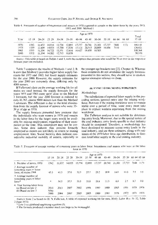
Table 4. Forecasts of number of brtummous coal mmers m 1970 expected to remain m the labor force by the years 1975. 1985. and 2000. Method I

Year

Age m 1970 Total

15-19 ‘t&24 25529 3&34 35-39 40-44 4549 5S-54 5559 60-64 6669 15569

1970 1542 11.632 14.855 13.734 12,893 17.237 20,741 21,301 17.237 7848 11’1 140.341 1975 1539 11,606 14,825 13.700 12.836 17.125 20,515 20,909 16,656 71 IO 136,821 1985 1533 11.554 14,723 13,551 12.614 16.627 19.459 18.303 108.364 2000 1512 11,304 14.202 12,713 10,839 50.570

Source: This table IS based on Tables I and 3. wtth the exception that persons who would be 70 or over in the respectwe forecast years are excluded.

Table 7 compares the results of Methods 1 and 2. It

is seen that Method 1 provides higher labor supply for-

ecasts for 1975 and 1985, but lower supply estimates for the year 2000. However, the supply estimates for the year 2000 are extremely close, differing only by 4086 mmers.

If Fullerton’s data on the average working life for all males are used instead, the supply forecasts for the years 1975 and 1985 come quite close to the Method 1 forecasts, but the year 2000 forecast is reduced to only 41.763. almost 9000 miners less than the Method 1 estimates. The difference is due to the total elimina- tion from the supply forecast of miners who were 35 39 yr of age in 1970.

The supply forecasts presented here presume that the individuals who were mmers in 1970 and remain in the labor force by the target years would be avail- able for mining employment, regardless of their occu- pation at the ttme. This assumption may not be cor- rect. Some data indicate that persons formerly employed as miners are not likely to return to mining employment, Also, Social Security data indicate con- stderable industrial mobility of miners, especially in

the younger age brackets (see [2], Chapter 4). Whereas these comments do not Invalidate the supply forecasts presented in this section, they should serve to caution against excessive reliance on them.

(B) ENTRY TO THE MINING WORKFORCE

Mrthorlolog?

The calculations of expected labor supply in the pre-

ceding sections ignored entry into the mining work-

force. But even if the mining workforce were to remain stable over a period of time, some entry must take place to replace workers separating from the mining workforce.

The Fullerton analysts is not suitable for determm- ing entry levels. Moreover, due to the special nature of the coal industry, entry levels specific to that industry should be computed. Therefore, a methodology has been developed to measure recent entry levels in the coal industry, and use these estimates, along with esti- mates of the 1970 labor force age distribution, to fore- cast total labor supply m the coal mining industry.

Table 5. Forecasts of average number of remammg years m labor force: brtuminous coal mmers who were m the labor force in 1970

Age m 1970 15-19 20-24 25-29 30-34 35-39 4&44 45-49 5G-54 55-59 6G64 65-69

1. Number of mmes. 1970 I542 11,632 14,855 13,734 12.893 17,237 20.741 31,301 17.237 7848 1121

2 Average number of remammg years m labor force, all males 1968 45.3 41.5 370 32.3 27.7 23.2 189 14.8 11.0 75 55

3 Average number of remaining years m labor force* t 54.5 37.5 35.5 33.0 19.8 11.5 6.0 25 0.7 00

4. Year leavmg labor force (a) Based on hne 2 2015 2011 2007 2002 1998 1993 1989 1985 1981 1978 1976 (b) Based on line 3 After

2000 2004 2007 2005 2003 1989 1981 1976 1972 1971 1970

Sources: Lme 2 1s based on H. N. Fullerton, A table of expected workmg lrfe for men, Mthly Labor Rrr. 51-52. Table 3 (June 1971)

* Lme 3 IS calculated employmg equation (5). 7 The formula produced a number much too large to be meanmgful.

Forrcastlng aggregate supply of coal rn~nw 297

Table 6 Forecasts of number of bltummous coal mmers m 1970 expected to remam m the labor force by the >ears 1\975, 19X5. and 2000 Method 2

Age m 1‘970 Year 15-19 20 23 75-29 x&34 35-39 4&U 45-39 5% 51 55 59 60 61 65 69 Total

1970 1542 Il.632 14.855 13.733 12.893 17.237 20.741 21.301 17.237 7X-N I121 1-10.1-11 1975 1541 11.632 14.855 13.734 12.893 17.237 20.741 21.301 I 13.935 19X5 1547 11.632 14,855 13.734 11,893 17.237 7 1 .x93 2000 1542 11.632 14.855 13,734 11.893 54.h56

Suurcr Tables I and 5

The analysis here is based upon two premises: first, It is assumed that the difference between the actual mining workforce m 1972 and the number of miners in 1968 expected to remam m the workforcc in 1972 (employing Method 1) is accounted for by new entries. Second. It 1s assumed that the entry levels by age observed during the period 1968%1973 will continue during the six 5-y’ periods from 1970 to 2000. When the new entries are added to the 1970 workforce expected to remam rn each target year, total labor sup- ply forecasts may be obtained.

In general. let the number of entrants of age x be denoted by NE,. Consider two periods. t and r - 1. Also, let x0 denote the youngest age bracket for which employment d;lta are available. Then one could de- scribe the workforce m years t and f - 1 as in Table 8. What the table implies is. first, that the number of workers of age x,, in year t are all new entrants (between the period t - I and t). Second, the work- force of persons aged x m year t IS composed of those who were of age .Y - 1 in year t - 1 and are remaining in the workforce at year t. plus any new entrants (between I - I and r). Given data on labor force by age for the two pcrlods. one could calculate L, , and L,_ , ,- , Usmp data for S, as explained above, the

Table 7. Summary of forecasts of number of bitummous coal mmers m 1970 expected to remam m the labor force

by the years 1975. 1985 and 2000

Year Forecastmg method I970 1975 1985 2000

I Method I l-IO.141 136.S21 108,363 50.570

2 Method 2 130.131 113.935 71.893 54.656

3 Based on average number of remamlng years m labor force for all males 110,131 140.141 113.035 -11,163

Sourcr~: Lme I IS based on Table 4. Line 2 1s based on Table 6, Lme 3 has been dewed from the InformatIon m Table 5, Lme &I.

*An example of the procedure IS probIded In 121. Table 9-10.

= L,., - L,._,,,_,(l - S,). for -1 > v,, (61

The total numbcr of new entrants IS simply the sum of the number of entrants over all age brackets.

Total number of entrants = x !VE,,. (7) in 1,

When the number of entrants is added to the number of the remaining workforce. as outlined m the previous section. an estimate of the total supply of miners for a given target date may be calculated

Table 9 presents the procedure employed to cstunate the number of new entrants mto the mining workforce during the period 196%1972. Line 1 gives the actual 196X employmrnt. by age. Lint 7 gives the numhcr of miners. by age. who were in the labor force in I Y6X and who are expected to remam m 1972. Lme 3 probidcs an estimate of the actual distribution of the mmmg workforce m 1972. The estimated number of entrants m lme 4 is obtained by subtractmg lme 2 from lint 3

Just as it was necessary to reduce the number of miners in 1970 by a separation rate or cvpcctrd work life into an expected labor force at a later year. so tt 1s necessary to reduce the numhsr ofentrants m a g~vcn period (say 1970-1975) into an expected component of the labor force m a later period (19X5 or 3)OO). The procedure chosen for that purpose IS the separation- rate analysis (Method I ) *

Employmg the acparation-rate proccdurc both for 1970 miners and new entrants. the expected labor SLIP-

ply in 1975. 1985 and 2000 is given in Table t 0. The

Table 8 C‘omponcnts of srparatmn from. and cntrh Into the coal mmlng workforce

Work force Age at At year jcar t t-1 At Icar t

-Y,l L,,, = 0 L,,, = .A.[:\,,

Y L,v, I_/ 1, = L,_ I,_,(I ~ s,j+ .VE,,

298 ELC’HANAN COHEU’. JON P. NEI.SON and GFOKG~ R. Nt c &tt~h

Table 9. Estimated number of entrants to the bitummous coal mmmg labor force, by age. lY68&1972

Age 15-19 ‘U 24 25-29 3@34 35_~39 4&W 45 -!9 5&51 55-59 60 64 65-69 To1aI

I. Labor force m 196X 639 6650 IO.232 10.743 17,662 18.928 21.358 12.381 15.987 7290 IO23 I77.XY3

2. 1968 Labor force expected to remam in 1972 Lme 1 x (1 - S,) 638 6635 10,313 10.716 12.606 18.80-l 11.125 21 Y6Y 15.438 606-I I241IX , 3 Labor force m 1972 1964 19.331 20.852 17.225 14.506 14.X0X 18,736 IV.492 15.713 7555 903 I 5 I. 100 4. Number of entrants. 1968- 1972, Lme 3SLme 2 1964 IX.703 13.237 7017 3790 7202 47,XxX

Sources. Line I personal commumcatlon by Lewis A. Brooker of the Umted Mme Workers of America Welfare and Retirement Fund, July 23, 1973. Lme 2: S, based on Table 2. Lme 3: Beneficlarles elgible for hospital and mcdtcal cart. Part C. Table 1, Umted Mme Workers of America Welfare and Retirement Fund. Washmgton. D.C (September 1972). and unpubhshed sources. Umted States Bureau of Mmes

table also provides an age dlstrlbution of the expected workforce. The labor supply in 1975 is estimated at 184,739, the 1985 forecast is 251,658 mmers, and for the year 2000 it is 334,467 miners.

The table illustrates the effect of the entry assump- tion on the distribution of the supply of miners in the forecast years. Whereas in the beginning of the period 1970~2000, the net effect of entry and separation is shown to increase the proportion of young workers. by the year 2000 the trend is reversed, indicating an in- crease in the proportion of older workers. This is due to the assumption of constant entry levels along with an increased work force during the period.

(C) PROBABILITY OF SHORTAGES

As noted earlier. demand forecasts for coal miners will not be explained here in detail. Our demand fore- casts of coal miners depend critically on assumptions concerning the following: (1) average productivity m surface and underground operations: (2) the per cent of coal mined in surface operations; (3) the average

number of days per year worked by coal mmers: and. (4) the anticipated demand for coal. Various methods have been employed to obtain values for those varl- ables for each forecast year. Considerable sensitivity has been found in the manpower demand forecasts for variations in the underlying assumptions. In Fig I are presented results of ‘probable’ and ‘high’ demand forecasts along with a summary of the supply forecasts. The ‘high’ demand forecasts are distinguished from the ‘probable’ demand forecasts only by variations in the assumption about anticipated coal production. Since the ‘probable’ and ‘high’ estimates of coal productlon for 1985 differ only by 64 mllhon tons, the manpower forecasts are not too dissimilar. For the year 3000. however. the high estimate of coal productlon (3 bll- lion tons) exceeds the probable estimate (1 blllion tons) by nearly 2 billion tons, resulting m sharply dlffurcnt manpOwer demand forecasts.

The data presented m Fig. I clearly indicate the remote likelihood of manpower shortages. if the pre- mises of the manpower supply and demand forccastmg techniques are accepted. The probability of shortages

Table 10. Forecasts of labor supply m the bltutnmous coal Industry. 1975, 1985 and 2000. emplo~mg method I fol actual 1970 workforce and assummg entry at each 5-yr interval 1s equal to the estimated 1968-197~ absolute levels. by age

l&19 2&24 25-29 3&34 35-39 4&43 45-49 5&54 55 -59 6&64 65-69 Total

1970 (Actual)

1547 11.632 14.885 13.734 12,893 17.137 10.74 I 21.301 17.237

7848 1121

Number 1975

(Per cent)

1964 (0.01) 1964 (0.00X) I964 mox) 70.732 (0 I I) 20.662 (0.08) 20.663 (0 Oh)

25.8’3 (0 14 34.835 (0.11) 34,x35 (0 10)

21,867 (0.12) 41.358 (0 16) 41.777 (0 12)

17.490 (0 09) 36.492 (0.15) 45.463 (0 14)

15.03X (0.0X) 27.692 (0. I 1) -17.465 (0 13) 17.135 (0.09) 19.487 (0 0x1 46.742 (0 14)

20.515 (0.1 I) 14.778 (0 06) 37.X65 (0.1 I)

‘0.909 (0 11) 16.627 (0.07) 36.7 I3 IO OS)

16,656 (0 09) 19.359 (0.0X) IX ‘X7 (0.M)

7110 (0 03) 1 x.303 (0.07) I2:h9X (0 04)

184.739 (100.0) 251.658 (1000) 334.467 ( I on 0)

Number 1YX5

(Per cent) Number 2000

(Per cent)

Forecasting aggregate supply of coal mmers 299

127 ,,

;, ,‘, :,,, : ,,,,, :

:, ,’ :‘,.

i

,,I ‘,, ,,’ ‘,‘, ,,

,/’ ,;, ,,; ,,

::.*;,,. :

POTENTIAL NEW ENTRANTS (IN THOUSANDS)

MINERS REMAINING FROM 1970 WORKFORCE (IN THOUSANDS)

MINERS DEMAND (IN THOUSANDS)

136

252 -

154

-

98

-

347 334

PROBABLE HIGH SUPPLY PROBABLE HIGH

DEMAND DEMAND FORECAST DEMAND DEMAND

FORECAST FORECAST FORECAST FORECAST

SUPPLY

FORECAST

1985 2000

Fig 1. Comparison of forecasts for bltummous coal mmmg of number of men demanded. probable and high levels with supply of men by source. Umted States, 1985 and 2000

IS considerable only if one accepts the premise of a

drastic change in the role of coal in the energy market over the next 25 yrs.

A serious difficulty with the interpretation of the supply forecasts presented hercm concerns the lack of wage and other working conditions variables in the model. It is imphcltly assumed throughout that wages and other workmg conditions m the coal industry will remain stable relative to other industries competing for the same type of workers. Changes in relative wages or working conditions could severely upset the supply forecasts reported m this study. Yet attempts to mcor- porate wage and working condltlons data into the model have not been successful, primarily because the nature of the available time-series data (which show a negative correlation between labor supply and wage rates [5]). Despito this and other difficulties with the approach. it appears that the methodology described m this paper offers a promising tool to forecast man- power supply in the coal (or any other) industry.

M. Sumansky provided outstandmg research asslstantship. Maureen C. Gallagher was responsible for much of the com- putatlonal work.

REFERENCES

E. Cohn. J. P. Nelson and G. R. Neumann, Forecastmg aggregate demand for coal mmers. Mlmce (1973). E. Cohn et u1., The demand for and supply of manpower m the bltummous coal industry for the years 1985 and 2000. Institute for Research on Human Resources, The Pennsylvama State University. Umverslty Park, Pa. (1973). (See especially Chapters 8 and IO) H N. Fullerton, A table of expected working hfe for men, 1968. Mtlzly Labor RCI, 49-55 (June 1971). Appalachian Reglonal CornmissIon, Manpower report for the Appalachian coal Industry (9 May 1973) E. Cohn. The demand for and supply of manpower in the bitummous coal Industry: prehminary forecasts for the years 1975, 1985 and 2000, Institute for Research on Human Resources, The Pennsylvama State Umverslt>, Umverslty Park, Pa. (1972).