forces in wingwalls from thermal expansion of skewed semi
TRANSCRIPT

Forces in Wingwalls from Thermal Expansion of
Skewed Semi-Integral Bridges
Eric Steinberg, Ph.D., P.E.
Shad Sargand, Ph.D.
for the Ohio Department of Transportation
Office of Research and Development
and the Federal Highway Administration
State Job Number 134267
November, 2010
Ohio Research Institute for
Transportation and the Environment

Form DOT F 1700.7 (8-72) Reproduction of completed pages authorized
12. Sponsoring Agency Name and Address
Ohio Department of Transportation1980 West Broad StreetColumbus, Ohio 43223
9. Performing Organization Name and Address
Ohio UniversityOhio Research Institute for Transportation and the EnvironmentDepartment of Civil Engineering Athens, OH 45701
4. Title and subtitle
Forces on Wingwalls from Thermal Expansion of Skewed Semi-Integral
Bridges
7. Author(s)
Eric SteinbergShad Sargand
13. Type of Report and Period Covered
15. Supplementary Notes
14. Sponsoring Agency Code
6. Performing Organization Code
8. Performing Organization Report No.
10. Work Unit No. (TRAIS)
11. Contract or Grant No.
134267
1. Report No.
FHWA/OH-2010/16
2. Government Accession No. 3. Recipient's Catalog No.
5. Report Date
November 2010
16. Abstract: Jointless bridges, such as semi-integral and integral bridges, have become more popular in recent years because of their simplicity in the construction and the elimination of high costs related to joint maintenance. Prior research has shown that skewed semi-integral bridges tend to expand and rotate as the ambient air temperature increases through the season. As a result of the bridge movement, forces are generated and transferred to the wingwalls of the bridge. ODOT does not currently have a procedure to determine the forces generated in the wingwalls from the thermal expansion and rotation of skewed semi-integral bridges. In this study, two semi-integral bridges with skews were instrumented and monitored for behavior at the interface of the bridge’s diaphragm and wingwall. A parametric analysis was also performed to determine the effects of different spans and bridge lengths on he magnitude of the forces. Based on the field results from the study it is recommended for the design of the wingwalls turned to run nearly parallel with the longitudinal axis of skewed semi-integral bridges should include a 100 psi loading at the wingwall/diaphragm interface from the thermal expansion of the bridge. In addition, analytical evaluations showed that longer spans and higher skews than allowed by ODOT’s BDM could be used. However, additional considerations for larger movements and stresses generated at the wingwall/diaphragm interface would need to be considered in designs. Finally, bearing retainers in diaphragms, if used, require adequate cover to avoid spalling of concrete.
18. Distribution Statement
No restrictions. This document is available to the public through the National Technical Information Service, Springfield, Virginia 22161
19. Security Classif. (of this report)Unclassified
20. Security Classif. (of this page)Unclassified
21. No. of Pages 22. Price
17. Key Words: Semi-intregral Bridge, Skewed Bridge, Wingwall, Thermal Expansion, Bridge rotation, and Bridge Diaphragm.

2
Forces in Wingwalls from Thermal Expansion of
Skewed Semi-Integral Bridges
Final Report
Prepared in Cooperation with the Ohio Department of Transportation,
U.S. Department of Transportation, and Federal Highway Administration
Principal Investigators: Eric Steinberg, Ph.D., P.E.
Shad Sargand, Ph.D.
Ohio University Ohio Research Institute for Transportation and the Environment
Department of Civil Engineering Athens, Ohio
The contents of this report reflect the views of the authors, who are responsible for the facts and accuracy of the data presented herein. The contents do not necessarily reflect the official views or policies of the Ohio Department of Transportation or the Federal Highway Administration.
This report does not constitute a standard, specification or regulation.
November, 2010

3
ACKNOWLEDGEMENTS The authors especially thank Jawdat Siddiqi, the ODOT technical liaison, for his insight and input related to the research. The efforts of former graduate student, Jibril Shehu, are also greatly appreciated. The assistance in instrumentation from Dr. Masada and research engineer Issam Khoury of Ohio University also deserve recognition.

4
TABLE OF CONTENTS
DISCLAIMER .......................................................................................................................2 ACKNOWLEDGEMENTS ...........................................................................................3 TABLE OF CONTENTS ................................................................................................4 LIST OF FIGURES ............................................................................................................5 LIST OF TABLES ..............................................................................................................7 1. INTRODUCTION .........................................................................................................8
1.1 Background .............................................................................................................8 1.2 Purpose ...................................................................................................................10 1.3 Objectives ..............................................................................................................11
2. LITERATURE REVIEW .....................................................................................12 2.1 Burke .......................................................................................................................12 2.2 Steinberg, Sargand, and Bettinger ...............................................................14 2.3 Ohio Department of Transportation ...........................................................16
3. FIELD EVALUATION ..........................................................................................19 3.1 Bridge Details .......................................................................................................19
3.1.1 DEF-24-0981 ........................................................................................19 3.1.2 MUS-16-0261 ......................................................................................20
3.2 Instrumentation ...................................................................................................25 3.2.1 DEF-24-0981 .........................................................................................25 3.2.2 MUS-16-0261 .......................................................................................34
3.3 Field Data ..............................................................................................................43 3.3.1 DEF-24-0981 ........................................................................................43 3.3.2 MUS-16-0261 .......................................................................................52
4. ANALYTICAL ASSESMENT ...........................................................................62 4.1 System Analysis ...................................................................................................62 4.2 Wingwall and Wall Abutment Interface ....................................................72
5. CONCLUSIONS .........................................................................................................80 6. RECOMMENDATIONS .......................................................................................81 7. REFERENCES .............................................................................................................85

5
LIST OF FIGURES Figure 1: Semi-Integral Abutment and Diaphragm (Side) ........................................................9
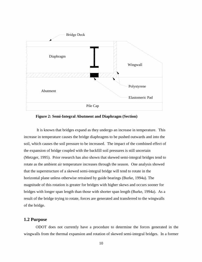
Figure 2: Semi-Integral Abutment and Diaphragm (Section) .................................................10
Figure 3: Horizontal Plane Rotation and Forces on Semi-integral Bridge ............................13
Figure 4: Abutment Type Limitations (Bridge Design Manual, 2007) ...................................17
Figure 5: Typical Cantilevered Wingwall .................................................................................18
Figure 6: Parallel Aligned Wingwall .........................................................................................18
Figure 7: DEF-24-0981 ................................................................................................................20
Figure 8: MUS-16-0261 Location ..............................................................................................21
Figure 9: Superstructure Framing Layout (MUS-16-0261).....................................................21
Figure 10: Abutment and Footing Section (MUS-16-0261) .....................................................22
Figure 11: Observed Distress of West Wall (West Bound Bridge) .........................................23
Figure 12: Observed Distress of East Wall (East Bound Bridge) ...........................................24
Figure 13: Propagated Cracks of West Wall (West Bound Bridge) .......................................25
Figure 14: Geokon Model VCE-4200 Vibrating Wire Strain Gage ........................................26
Figure 15: Vibrating Wire Strain Gage Installation ...............................................................27
Figure 16: Vibrating Wire Strain Gage Tied to Reinforcement .............................................28
Figure 17: Vibrating Wire Strain Gage Locations ..................................................................29
Figure 18: Geokon Model GK-401 Microprocessor ................................................................31
Figure 19: Fluke 87 Series III True RMS Multimeter ............................................................32
Figure 20: Digimatic Indicator Targets Location ....................................................................33
Figure 21: Top view of Mitutoyo Model IDC112T ABSOLUTE Digimatic Indicator .........33
Figure 22: Calibration Plate with Metal Targets .....................................................................34
Figure 23: Instrumentation (East Bound Bridge) ....................................................................35
Figure 24: Instrumentation (West Bound Bridge) ...................................................................35
Figure 25: Target Location (East Bound Bridge) ....................................................................36
Figure 26: Target Location (West Bound Bridge) ...................................................................37
Figure 27: Tilt Reference Stations (East Bound Bridge) .........................................................38
Figure 28: Tilt Reference Stations (West Bound Bridge) ........................................................39

6
Figure 29: Field Set-Up for Data Acquisition (Masada, 2007) ...............................................40
Figure 30: Digi-tilt Sensor and Readout Device (Masada, 2007) ............................................41
Figure 31: Reference Plate on Wall Abutment (Masada, 2007) .............................................41
Figure 32: Digital Strain Meter .................................................................................................43
Figure 33: Average Wingwall Stress vs Average Internal Temperature (DEF-24-0981) ....45
Figure 34: Wingwall Stress – S Gages (DEF-24-0981) ...........................................................47
Figure 35: Wingwall Stress – B Gages (DEF-24-0981) ...........................................................47
Figure 36: Average Wingwall Stress (DEF-24-0981) ...............................................................48
Figure 37: Interface Gap vs Average Wingwall Stress (DEF-24-0981) .................................50
Figure 38: Interfacce Gap vs Average Temperature (DEF-24-0981) ....................................52
Figure 39: Joint 1 Gap versus Average Temperature (East Bound MUS-16-0261) .............57
Figure 40: Joint 1 Displacement vs Average Temperature (East Bound MUS-16-0261)......58
Figure 41: Deck Divided into Rhombus Shell Elements .........................................................63
Figure 42: Resistance Modeled with Linear Springs ...............................................................64
Figure 43: Span Length on Stresses for Different Skews (kEq = 35.7lb/in3) ..........................69
Figure 44: Span Length vs Stresses for Different Skews (kEq = 100.57lb/in3) .......................70
Figure 45: Span Length vs Stresses for Different Skews (kEq = 165.75 lb/in3) ......................70
Figure 46: Wingwall and Wall Abutment Model .....................................................................73
Figure 47: Wall and Backfill ......................................................................................................74
Figure 48: Wall Abutment and Wingwall Deformation ..........................................................76
Figure 49: Front Side Stresses (ksi) ...........................................................................................77
Figure 50: Backside Stresses (ksi) .............................................................................................78
Figure 51: Front side Stresses (ksi) ...........................................................................................79
Figure 52: Wingwall Detail (DEF-24-0981) ..............................................................................81
Figure 53: Wingwall Detail (MUS-16-0261) .............................................................................83
Figure 54: Bearing Retainer (MUS-16-0261) ...........................................................................84

7
LIST OF TABLES
Table 1: Average Stresses and Temperatures .....................................................................44
Table 2: Digimatic Target Readings (DEF-24-0981) .........................................................49
Table 3: Internal Temperatures and Joint Gap (East Bound MUS-16-0261) .................54
Table 4: Change in Internal Temperatures and Joint Displacements (East Bound MUS-
16-0261) ..................................................................................................................................54
Table 5: Internal Temperatures and Joint Gap (West Bound MUS-16-0261) ................54
Table 6: Change in Internal Temperatures and Gap Displacements (West Bound MUS-
16-0261) ..................................................................................................................................55
Table 7: Abutment and Wingwall Tilt (East Bound MUS-16-0261) ................................59
Table 8: West Abutment and Wingwall Tilt (West Bound MUS-16-0261) .....................59
Table 9: Abutment and Wingwall Tilt Changes (East Bound MUS-16-0261) ................60
Table 10: Abutment and Wingwall Tilt Changes (West Bound MUS-16-0261) .............61
Table 11: Equivalent Stiffness to Spring Stiffness Conversion ........................................65
Table 12: PEJF Test Results ................................................................................................67
Table 13: Forces and Stresses in East Wingwall ................................................................67
Table 14: Forces and Stresses in West Wingwall ...............................................................68
Table 15: Analytical Wall Joint Movement (45o skew and Span = 139 ft.) .....................71

8
CHAPTER 1: INTRODUCTION
1.1 Background Bridges that utilize expansion joints have increased the overall maintenance cost
of bridges due to leakage at the expansion joint. One of the major causes of expansion
joint deterioration is observed when water carrying de-icing salts leaks through the
expansion joints. The de-icing salts cause an increased rate of corrosion of the joint, as
well as structural components beneath the joint including the superstructure and
substructure.
However with the introduction of the jointless bridges such as semi-integral and
integral bridges, the high joint maintenance cost is eliminated. In addition, the added
simplicity in the construction of integral and semi-integral bridges has led them to
become more popular in recent years (Bettinger, 2001). Oesterle and Lotfi (2005) also
confirmed that in addition to reduced maintenance cost, jointless bridges improve riding
quality, promote lower impact loads, reduce snowplow damage to decks and approach
slabs, as well as improve the seismic resistance of the bridge.
Integral bridges are those designed such that the superstructure (deck, girder and
diaphragm) are rigidly connected to the substructure through bonded construction joints
between the diaphragm and abutment and at the abutment/foundation interface
(Steinberg, Sargand, and Bettinger, 2004). Longitudinal expansion/contraction of the
bridge is taken in foundation and the bridge behaves similar to a frame.
In semi-integral bridges, the deck, girders, approach slab, and diaphragm act
together as a single unit. Flexible bearing surfaces such as elastomeric pads are used in
place of the bonded construction joints used for integral abutment bridges. A semi-
integral bridge is illustrated in a side view (Figure) and section view (Figure). The
flexible bearing surfaces provide more flexibility at diaphragm/abutment interface. Thus
the magnitude of the forces transferred to the foundation is theoretically decreased
(Steinberg, Sargand, and Bettinger, 2004). In order to prevent unwanted materials such
as soil and aggregates from restraining the movement of the diaphragm/abutment joint

9
and diaphragm/wingwall joint, polystyrene is used to fill the joint’s gap. The structural
behavior of these types of bridges is affected by both the temperature changes and
loading conditions imposed on the bridges.
Approach SlabBridge Deck
BackfillGirder
Diphragm
Polystyrene
Elastomeric Pad
Abutment
Pile Cap
Fill
Figure 1: Semi-Integral Abutment and Diaphragm (Side)
10
Figure 2: Semi-Integral Abutment and Diaphragm (Section)
It is known that bridges expand as they undergo an increase in temperature. This
increase in temperature causes the bridge diaphragms to be pushed outwards and into the
soil, which causes the soil pressure to be increased. The impact of the combined effect of
the expansion of bridge coupled with the backfill soil pressures is still uncertain
(Metzger, 1995). Prior research has also shown that skewed semi-integral bridges tend to
rotate as the ambient air temperature increases through the season. One analysis showed
that the superstructure of a skewed semi-integral bridge will tend to rotate in the
horizontal plane unless otherwise retrained by guide bearings (Burke, 1994a). The
magnitude of this rotation is greater for bridges with higher skews and occurs sooner for
bridges with longer span length than those with shorter span length (Burke, 1994a). As a
result of the bridge trying to rotate, forces are generated and transferred to the wingwalls
of the bridge.
1.2 Purpose ODOT does not currently have a procedure to determine the forces generated in the
wingwalls from the thermal expansion and rotation of skewed semi-integral bridges. In a former
Diaphragm
Wingwall
Abutment
Pile Cap
Elastomeric Pad
Polystyrene

11
study, it was determined that these thermal forces can be significant. However, this study
examined a bridge with a minor skew and wingwalls that were parallel to the diaphragm of the
bridge. In addition, the instrumentation used to measure the forces was localized in a relatively
small area of the wingwall and may not have provided a representation of the forces existing
over the height of the wingwall. Larger skews and longer spans may produce even larger forces.
The effects of the stiffness of the backfill behind the diaphragm and the approach slab on the
magnitude of the forces transferred to the wingwalls is also not fully understood
Wingwalls that are parallel to the diaphragm of the bridge are subjected to an axial force
from the thermal movement. ODOT is now utilizing more wingwalls that are turned back and
run perpendicular or nearly perpendicular to the diaphragm. Wingwalls that are turned back
would be subjected to bending from the thermal movement in addition to the axial force.
Stresses from the combined bending and axial forces could be critical in the design of the
wingwall.
1.3 Objectives The main focus of this research project was to utilize the results of field
assessments, as well as a computer analysis, in order to achieve the following:
- Evaluate conditions of wingwalls and wall abutments
- Asses the cause of the observed distress in the walls
- Monitor the movement of the bridges due to temperature changes
- Begin to develop guidelines to assist in achieving improved design of skewed
semi-integral bridges
- Improve the understanding of the soil-structure interaction between
superstructure, substructure, and embankment soil due to changes in
temperature
To meet these objectives, the two skewed semi-integral bridges bridges were located
in the northern and central Ohio were instrumented and analyzed in this project. In
addition a parametric study was performed to assess other parameters affecting the
bridge’s behavior.

12
CHAPTER 2: LITERATURE REVIEW
The amount of research conducted on the design and behavior of skewed semi-
integral bridges due to thermal expansion is very limited. As such, information
pertaining to the effect it has on wingwalls and foundations is difficult to obtain.
Substantial amount of research work however, has been done on the pressures and forces
acting on the abutment of skewed integral bridges due to thermal expansion (Bettinger,
2001).
2.1 Burke
Martin P. Burke has documented his research work conducted on the longitudinal, lateral,
and rotational movement of semi-integral bridges in several publications (Burke, 1994A.; Burke,
1994B; and Burke and Gloyd, 1994). His most recent publication summarizes previous work on
semi-integral, as well as, integral bridge behavior (Burke, 2009). An insight on the behavior of
skewed semi-integral bridges due to thermal expansion can be gained by making reference to
Figure. In response to a rising temperature of the superstructure in a semi-integral bridge, an
elongation (ΔL) is experienced by the bridge. The backfill in turn reacts to produce resistive
compressive passive soil pressures on both diaphragms of the bridge. The resultant of these
compressive passive soil pressures is denoted by PP. Thus, a force PE is developed in the bridge
as a result of the expansion. The generated force PE of a skewed semi-integral bridge with skew
angle θ is resisted by the longitudinal component (PPsecθ) of the resisting compressive passive
force (PP) of the soil being compressed behind the diaphragms. The lateral component (PPtanθ)
of the resisting passive force helps to resist the frictional backfill force (PPtanδ).

13
Figure 3: Horizontal Plane Rotation and Forces on Semi-integral Bridge
In skewed semi-integral bridges, Burke noted the resultant forces of the passive
soil pressures developed at both ends of the bridge due to longitudinal expansion of the
bridge are not concurrent. A moment couple is therefore produced from the non-
concurrent forces that could potentially lead to the rotation of the bridge towards its acute
corners in the manner shown in Figure. In order for the superstructure of a skewed semi-
integral bridge to be stable, the force couple system that is causing rotation as described
above must be resisted by an equivalent force couple system. This can be stated in
Equation (1) as:
Pp Lsinθ ≤ Pp tanδ Lcosθ (1) where: Pp Lsinθ = Force couple developed from the passive soil pressure behind the diaphragm Pp tanδ Lcosθ = Frictional resistive between the diaphragm and soil force couple
Burke found that using reasonable values of a factor of safety of 1.5 and a 22o
angle of friction, δ, between the diaphragm/soil interface results in a stable system if the
bridge’s skew is < 15o. For bridge skews larger than 15o, rotation will likely be initiated

14
unless guide bearings are provided. In addition Burke has noted that once rotation is
initiated, soil pressure behind the diaphragm will be increased at the bridge’s obtuse
corner and reduced at the acute corners. This will shift the resultant force from the soil
pressures and reduce the force couple tending to cause the rotation. Therefore, rotational
movements would be reduced during accompanying thermal cycles. However, the
rotation would continue to produce cumulative effects until the movement is restrained
by other means.
2.2 Steinberg, Sargand, and Bettinger
Field and analytical research related to skewed semi-integral bridges carried out
by Steinberg, Sargand and Bettinger can be found in several references (Steinberg,
Sargand, and Bettinger, 2004; Steinberg and Sargand, 2001; and Bettinger, 2001). This
research was conducted to determine the forces exerted in the wingwalls of skewed semi-
integral bridges in Athens County and Tuscarawas County, Ohio. The research was
conducted with the aim of gaining a better understanding of the effect that changing
ambient temperature has to the forces exerted on the wingwalls of skewed semi-integral
bridges. The wingwall/abutment joints of two bridges in Ohio were instrumented to
monitor the movement of the bridges as well as the forces generated in the wingwalls due
to thermal expansion. The Tuscarawas County bridge had a single span length of 87ft
and a roadway width of 32ft with a skew angle of 65o. It was made up of composite
reinforced concrete deck supported by steel girders. The backfill material for this bridge
was sandy soil. The Athens County Bridge however, was a four span continuous steel

15
girder semi-integral bridge, also with a composite reinforced concrete deck. The outer
and inner spans were 70ft and 87ft long, respectively. The roadway width was 40ft wide
and the skew angle was 25o.
In addition to the instrumentation of the bridges, computer analysis was carried
out in order to validate the data collected in the field. SAP 2000 was used to model the
Athens County bridge to determine the forces generated and exerted on the wingwalls. In
addition, bridges were analyzed with multiple skew angles and span lengths in order to
determine the impact a greater skew or longer span length has on the forces generated
against the wingwalls.
The research discovered that significant wingwall force up to a maximum of 35.7
kips in magnitude was experienced by the Tuscarawas County bridge and up to a
maximum of 30.1 kips in magnitude was experienced by the Athens County bridge
during the course of the study. It should also be noted that the instrumentation to
measure the forces was limited to a small area of the wingwall/diaphragm interface. The
maximum longitudinal movement recorded for the Athens County bridge was 0.6442 in.
and a maximum movement into the wingwall of 0.1295 in. was also measured. Based on
the data recorded, direct correlation between the ambient temperature and the generated
forces for the bridges did not exist or was limited. Nonlinear relationships existed
between the wingwall/diaphragm interface joint movement and the force generated in the
wingwall.
Analytical results revealed that as the bridge skew angle increases, so does the
force generated in the wingwall. Also for a larger skew angle, the increase in the

16
wingwall force was higher as the backfill stiffness increased. Based on this work
Equation (1) was modified to include the effects from the wingwalls as shown in
Equation (2).
Pp Lsinθ = Pp tanδ LCosθ + (additional force couple from wingwalls) (2) 2.3 Ohio Department of Transportation
With the principal goal of eliminating the bridge deck joints, designers in the state
of Ohio adopted the design of continuous integral concrete bridges and continuous
integral steel bridges which began over 6 decades and 3 decades ago, respectively
(Burke, 1994B). There were however, few exceptions in the sense that joints were
provided at the ends and center of bridges with span length longer than 600ft. In
addition, bridges with a skew angle greater than 30o, those longer than 300ft, curved
bridges, and those with wall or stub abutments were also provided with joints. The
inadequate functional quality and durability of the provided deck joint sealing systems
and the constant maintenance associated with it caused designers in Ohio to innovate
ways of combining the attributes of integral construction to those of bridges with
movable joints (Burke, 1994B). As a consequence, the semi-integral bridge design
concept was adopted. Prior to the development and adoption of semi-integral bridges, the
application range of deck-jointed bridges was limited to 400ft span length with no skew
or 200ft span length with a maximum skew angle of 30o. With the introduction of semi-
integral bridges however, the limits were expanded to the extents shown in Figure
(Burke and Gloyd, 1994). Several characteristics outlined by Burke (1994b) need to be

17
recognized and provided for by design engineers. However, for the purpose of this thesis,
only longitudinal, lateral and rotational restraint were discussed.
Figure 4: Abutment Type Limitations (Bridge Design Manual, 2007)
In the state of Ohio, wingwalls are currently designed to act only as retaining
walls for the adjacent embankment soil (Bridge Design Manual, 2000). The forces
exerted on the wingwalls by the superstructure due to thermal expansion are not
considered. Wingwalls have typically cantilevered out from the bridge along the skew of
the bridge (see Figure 5). However, wingwalls are recently being constructed more in a
parallel alignment (turned back position) to the bridge longitudinal axis (see Figure 6).
The parallel alignment (turned-back position) of the wingwall provides an additional

18
longitudinal restraint by way of backfill/wingwall friction or shearing resistance of
backfill for wingwalls with rough surfaces due to the increase in confining pressure
imposed by the turned back wingwalls (Burke, 1994B). However, it is important to note
that the wingwall now becomes more subjected to bending stresses (Figure 6) than axial
compression (Figure 5) from rotation of a skewed bridge.
Figure 5: Typical Cantilevered Wingwall
Figure 6: Parallel Aligned Wingwall

19
CHAPTER 3: FIELD EVALUATION
Part of the research in this project involved monitoring bridge in two different
geographical locations in Ohio. One bridge was located in northeastern Ohio near the city of
Defiance. The other bridge location was in central Ohio near the city of Newark. This chapter
discusses the details of the bridges and the associated field evaluations.
3.1 Bridge Details
3.1.1 DEF-24-0981 This bridge location was on US-24 over the Tiffin River near Defiance, Ohio. Though
two similar bridges exist at this location, only the westbound bridge was instrumented and
studied. Construction began on the bridge in May 2006. The bridge is a four-span 440-foot
composite structure with outside spans of 120 feet and inside spans of 100 feet. It has a skew of
45 degrees and features six 72-inch Modified AASHTO Type IV prestressed concrete I-beams.
The roadway width is 42’-0” from toe-to-toe of the parapet wall barriers. The reinforced
concrete deck is 8½” thick between girders and 10½” thick over the girders. The approach slabs
are 30 feet long and 17 in. thick. The bridge’s substructure includes semi-integral abutments and
drilled shaft foundations. The wingwalls run parallel to the bridge. The wingwall at the acute
corner of the rear abutment for the westbound bridge was instrumented. This wingwall was 18
in. thick, over 18 feet in length, and more than 8 feet high. Seismic pedestals exist at the piers
but no guide bearings existed at the abutments.
The concrete for the instrumented wingwall was poured on November 29, 2006.
Placement of the concrete for the deck and diaphragm was completed on May 18, 2007. The
backfill behind the wingwall was placed in early June of 2007, and the approach slab was poured
in late June of 2007. Bridge construction was completed and the two westbound lanes opened to
the public in August 2007. Figure 7 shows the completed bridge.

20
Figure 7: DEF-24-0981
3.1.2 MUS-16-0261 This location actually consisted of two nearly identical bridges for east and west
bound State Route 16 located in Muskingum County, Ohio. Both of these bridges were
instrumented some time after their completion. The bridges were part of a project which
involved the upgrading of a 2.36 mile stretch of S.R 16 (see
Figure 8) from a two lane to four lane highway. The bridges pass over Raiders
Road and were opened to traffic in 1998.

21
Figure 8: MUS-16-0261 Location
The east and west bound single span bridges have a total span length of 140ft and 139ft
from center to center of bearing, respectively. The bridges are 42ft wide from toe to toe of
barriers. They are both semi-integral bridges with a skew angle of 45o. The deck is 9 in. deep
and is made of 4.5ksi reinforce concrete. Approach slabs on both ends of the bridge are 25ft
long. Figure 9 shows the superstructure framing layout of the west bound bridge. The girder
sections of the bridges are grade 50 ASTM A572 welded steel plate girders spaced 10ft apart.
Figure 9: Superstructure Framing Layout (MUS-16-0261)
Project Location

22
The girders are supported on short HP sections and bearing pads. The outside girders
also have a bearing retainer assembly at the bearing pads to resist transverse movement of
the girders. The bearing pads are supported by 19.1ft high wall abutments at each end of
the bridge. As can be seen from Figure 10, the wall abutments are supported on a 3ft deep
by 14.5ft wide 4 ksi concrete strip footing without any deep foundation. The wall
abutments, which span the full width of the bridge, are tapered from 3ft at the top to 4 ft.
at the bottom with the bridge span side of the wall being vertical.
Figure 10: Abutment and Footing Section (MUS-16-0261)

23
After the bridge was open to traffic, signs of distress were observed as cracks at
the abutment/wingwall interface of the west wall of the west bound bridge as well as the
east wall of the east bound bridge. Pictures of the observed distresses are shown for the
west wall (Figure 11) and the east wall (Figure 12), respectively. Initially, the cracks
were patched but only proved to resurface again. Over time, the cracks were observed to
have propagated as shown in Figure 13.
Figure 11: Observed Distress of West Wall (West Bound Bridge)

24
Figure 12: Observed Distress of East Wall (East Bound Bridge)

25
Figure 13: Propagated Cracks of West Wall (West Bound Bridge) 3.2 Instrumentation
3.2.1 DEF-24-0981
Two types of instrumentation were utilized for this bridge. Geokon Model VCE-4200
Vibrating Wire (VW) Strain Gages were used to measure both strain and temperature inside the
wingwall. These VW strain gages are specifically designed for direct embedment in concrete.
The Geokon VCE-4200 VW strain gage has a gage length of approximately 6 in (150 mm), a
standard range of 3000 microstrains (με), a resolution of 1.0 με, and a temperature range of -68°F
(-20°C) to 176°F (80°C). The VW strain gage is commonly used to measure strain in

26
foundations, piles, bridges, dams, and similar structures and utilize the vibrating wire principle to
measure strain. This principle involves a length of steel wire is tensioned between the two end
blocks of the gage, which is directly embedded in concrete. Deformations, or strain changes,
inside the concrete structure causes the two end blocks to move relative to one another. These
changes in strain affect the amount of tension held in the steel wire. This tension is then
measured by electronically plucking the wire and measuring its resonant frequency of vibration
with the use of an electromagnetic coil inside the gage. The vibrating wire strain gages are
primarily designed for long-term strain measurement and thus are not suitable for measuring
dynamic strains. The gages are also fully waterproof. Figure 14 depicts one of these strain
gages along with its connected wiring which allows for measurement of both strain and
resistance in the vibrating wire contained in the gage.
Figure 14: Geokon Model VCE-4200 Vibrating Wire Strain Gage
Strain gage instrumentation took place after reinforcing steel was placed in the wingwall
but before the concrete was poured. Vibrating wire strain gages were attached to the wingwall
reinforcing bars with the use of steel wire and duct tape in a manner such that the installation

27
allowed strain measurements within the concrete. Figures 15 and 16 show the installation of the
VW strain gages in the wingwall.
Figure 15: Vibrating Wire Strain Gage Installation

28
Figure 16: Vibrating Wire Strain Gage Tied to Reinforcement
A total of eight VW strain gages were installed in the wingwall. All of the gages were
oriented perpendicular to the face of the wingwall in order to measure the strains placed on
the wingwall as a result of thermal expansion and contraction of the bridge. As seen by the
plywood form in Figure 16, the gages were all placed approximately 1” from the edge of the
wingwall nearest the diaphragm. The eight VW strain gages were placed in two columns of four
gages. One column of gages were installed as close as possible toward the bridge and other
column of gages was closer to the approach slab. The locations of the gages in relation to each
other have also been are shown in Figure 17. Although not noted in the diagram, the top of the
wingwall is located at a height of approximately 8’3” above the base. The vibrating wire strain
gages were labeled based on their location with respect to height and to which end of the bridge
each was closest. The left column of four gages was designated the soil (S) side, whereas the
four right-hand gages were labeled as bridge (B) side gages. The labeling with respect to
elevation (TOP, MIDT, MIDB, and BOT) can also be seen in Figure 17. The installation of VW

29
strain gages was completed in November 2006, and the concrete for the wingwall was poured the
following week.
Figure 17: Vibrating Wire Strain Gage Locations
Strain measurements of the vibrating wire strain gages were taken using a Geokon
Model GK-401 Microprocessor as shown in Figure 18. The measurement output was in
units of microstrain. However, the strain has to be corrected for temperature in order to account
for the strain only due to loading. The corrections are necessary due to slight differences in the
thermal coefficients of the gages and the concrete. Equation (3) was used to determine the strain
from loading.
Base of Wingwall
2’3”
1’10.5”
2’2”
1’2”
1’9”
2’3.2”
2’1”
1’4.3”
1’4.3”
1’5.5”
1’5.8”
1’6.2”
1’11.8”
1’10”
1’9.5”
1’8.3”
Front of Wingwall
TOP
MIDT
MIDB
BOT
Soil(S) Bridge(B)
4’3”
Back Edge of Diaphragm
30
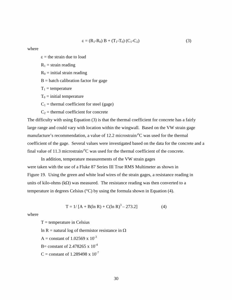
ε = (R1-R0) B + (T1-T0) (C1-C2) (3)
where
ε = the strain due to load
R1 = strain reading
R0 = initial strain reading
B = batch calibration factor for gage
T1 = temperature
T0 = initial temperature
C1 = thermal coefficient for steel (gage)
C2 = thermal coefficient for concrete
The difficulty with using Equation (3) is that the thermal coefficient for concrete has a fairly
large range and could vary with location within the wingwall. Based on the VW strain gage
manufacture’s recommendation, a value of 12.2 microstrain/oC was used for the thermal
coefficient of the gage. Several values were investigated based on the data for the concrete and a
final value of 11.3 microstrain/oC was used for the thermal coefficient of the concrete.
In addition, temperature measurements of the VW strain gages
were taken with the use of a Fluke 87 Series III True RMS Multimeter as shown in
Figure 19. Using the green and white lead wires of the strain gages, a resistance reading in
units of kilo-ohms (kΩ) was measured. The resistance reading was then converted to a
temperature in degrees Celsius (°C) by using the formula shown in Equation (4).
T = 1/ [A + B(ln R) + C(ln R)3 – 273.2] (4)
where
T = temperature in Celsius
ln R = natural log of thermistor resistance in Ω
A = constant of 1.02569 x 10⁻³
B= constant of 2.478265 x 10⁻⁴
C = constant of 1.289498 x 10⁻⁷

31
The formula in Equation (4) was provided in the specifications for the Geokon Model
VCE-4200 Vibrating Wire Strain Gages. Finally, the Celsius temperature was then converted to
degrees Fahrenheit (°F) using Equation (5).
T°F = 1.8 T°C + 32°F (5)
where
T°F = temperature in degrees Fahrenheit
T°C = temperature in degrees Celsius
Figure 18: Geokon Model GK-401 Microprocessor

32
Figure 19: Fluke 87 Series III True RMS Multimeter
In addition to the VW strain gages, digimatic indicator targets were used to monitor the
expansion and contraction of the joint between the diaphragm and wingwall. The 1 ½” long
stainless steel targets were permanently embedded in the concrete, while the 5/8” steel screws
are threaded into the targets in order to take measurements. By using the embedded targets, the
digimatic indicator is able to measure movement towards and away from the wingwall at a high
accuracy. Installation of the digimatic indicator targets originally occurred on the top surface of
the wingwall and diaphragm soon after the concrete was poured. However, due to the placement
of a parapet wall in the location of these targets, new targets had to be installed in late August of
2007 at the vertical face of the wingwall-diaphragm interface. The digimatic indicator targets
are located on each side of the expansion joint material between the wingwall and diaphragm. A
diagram of the targets and their labeling can be seen in Figure 20. Target rows two and three
were the original two locations of the targets. However, due to the limited range of the digimatic
indicator device, rows one and four were installed in October 2007 in order to properly take
readings with the indicator.

33
Figure 20: Digimatic Indicator Targets Location
The digimatic indicator target readings were taken with a Mitutoyo Model IDC112T
ABSOLUTE Digimatic Indicator (see Figure 21). The indicator has a range of ±0.5 inches and
an accuracy of 0.00012 inches. Readings were taken as a digital readout of four decimal places.
In addition, one of the contact points on the indicator can be adjusted so that five different 0.5
inch ranges between approximately 1.7 and 10.24 inches can be used. Each time this contact
point was moved, the steel calibration plate shown in Figure 22 was used to calibrate the
digimatic indicator to the proper range for data collection.
Figure 21: Top view of Mitutoyo Model IDC112T ABSOLUTE Digimatic Indicator

34
Figure 22: Calibration Plate with Metal Targets
3.2.2 MUS-16-0261
These particular bridges were instrumented because of the signs of distress they displayed
and the uniqueness of their abutment walls on a shallow foundation. It should also be noted that
instrumentation was installed long after construction was completed negating internal sensors
from being installed and resulting in difficulties of interpreting data. The wingwalls of the
outside acute corners of both of bridges were instrumented because they showed signs of distress
and wingwalls did not exist on the acute corners between the bridges due to the continuous
abutment walls between the bridges. The wall abutments near the instrumented
wingwall/diaphragm interfaces were also instrumented to monitor their tilt which was suspected
to be due to either differential settlement and/or thermal effects. Thermal were installed to
measure internal temperatures. A plan view of the instrumentation can be seen in Figure23 and
24.

35
Figure 23: Instrumentation (East Bound Bridge)
Figure 24: Instrumentation (West Bound Bridge)
The outside acute corners were instrumented to determine the effect thermal
expansion/contraction of the bridges had on the wingwall/diaphragm interface joint. Digimatic
indicator metal targets (see Figure 22) were installed on the walls of the bridges on each side of
the wingwall/diaphragm interface joint. To install the metal targets, the desired distance between
the two targets was measured, and holes were drilled at those locations. The concrete particles
from the drilling were cleaned out of the holes to ensure a strong bond between the metal targets

36
and the concrete. The targets were then embedded into the walls and held in place with the use
of a rapid setting two part epoxy. For the east bound bridge, two sets of targets were installed
8in and 10in apart, while on the west bound bridge only one set of targets installed 8in apart was
used. Figures 25 and 26 show the approximate locations of the targets. The installation of the
west bound bridge metal targets was done several months after the initial installment of
instrumentation due to difficulties in gaining access to the height of the desired location. In
addition to that, the topography of the ground surface adjacent to the location at which the
installation was to take place was very steep and considered dangerous for the installation crew.
Figure 25: Target Location (East Bound Bridge)

37
Figure 26: Target Location (West Bound Bridge)
The expansion and contraction measurements were taken with the Mitutoyo Model
IDC112T ABSOLUTE Digimatic Indicator (see Figure 21). Prior to any measurements, the
Digimatic Indicator was calibrated to the appropriate target spacing, 8in or 10in. A decrease in
the pre-set gauge length indicated expansion of the bridge while an increase in the gauge length
indicated contraction of the bridge.
The measuring of the angle of tilt for the wingwalls and abutments was attained by
establishing measurement stations on the bridges. A total of six stations were set up with three
stations on each bridge. Figures 27 and 28 show the locations at which the stations were
established on the walls of each bridge. The reference points circled in black with the arrow

38
pointing to the left were located further to the left in the picture. For each bridge, one station
was established on the wingwall and the other two were established on the wall abutments.
Figure 27: Tilt Reference Stations (East Bound Bridge)

39
Figure 28: Tilt Reference Stations (West Bound Bridge) In order to establish a reference station, a rebar locator was used to determine the location
of the rebars in the walls. This was done in order to assure availability of depth into the walls up
to 2 in., as well as to prevent drilling into the rebars and possibly decreasing the structural
integrity of the wingwalls or wall abutments. A vertical distance of 2.5 ft. was measured
between the two points at which holes were drilled. The concrete particles were cleared after
drilling to establish proper bond between the concrete and the stainless steel reference points.
Using a quick setting two-part epoxy, two stainless steel reference points were embedded 2 in.
into the concrete wingwall or wall abutment at each station.
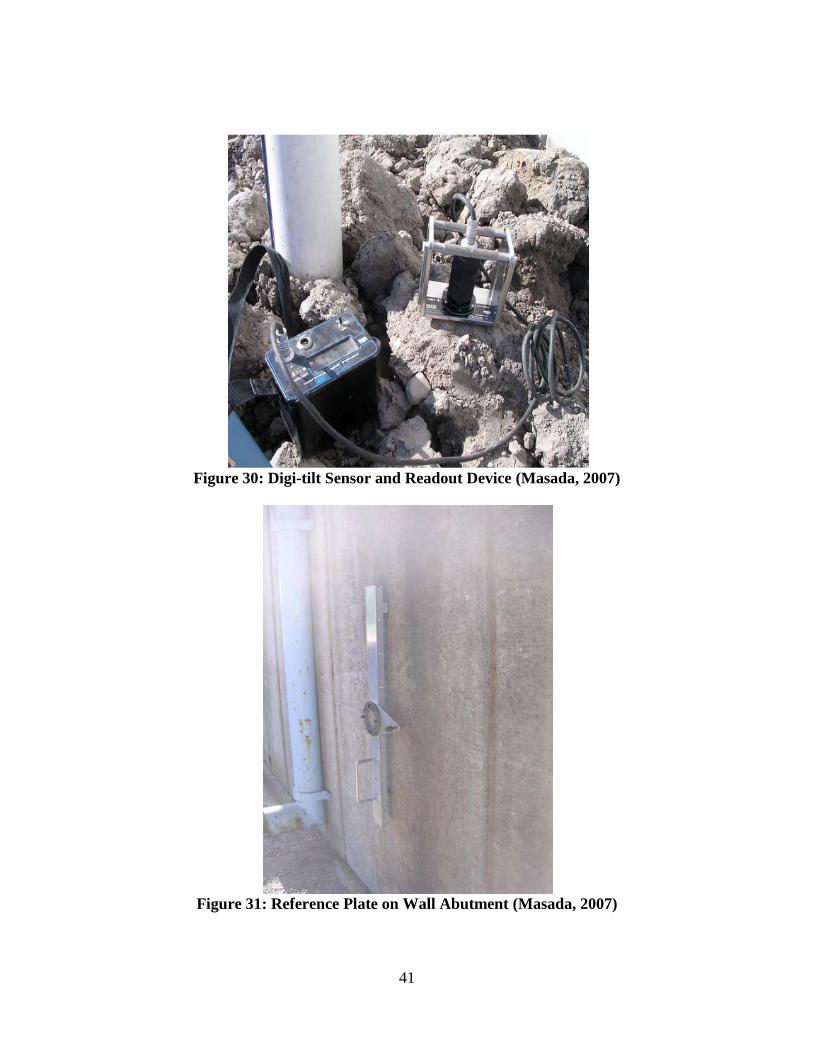
The Digi-Tilt tiltmeter manufactured by Slope Indicator (Seattle, Washington) was used
in the tilt measurements. The system comprises of a accelerometer sensor and a digital readout
device. In order to take a tilt reading at a given measuring station, a stainless steel ball on a
threaded shaft was screwed into each of the established reference points. A reference plate was

40
then positioned and held against the steel joints, and with the use of an accelerometer, readings
were taken. The field set up for the data acquisition is illustrated in Figure 29. In addition,
Figure 30 shows the components of the data acquisition equipment (readout device and
accelerometer) while Figure 31 shows the reference plate hanging on the wall.
Figure 29: Field Set-Up for Data Acquisition (Masada, 2007)
41
Figure 30: Digi-tilt Sensor and Readout Device (Masada, 2007)
Figure 31: Reference Plate on Wall Abutment (Masada, 2007)

42
According to Masada (2007), the tilt-meter sensor has a range from -30o to +30o and a
sensitivity of 0.003o. One single measurement using the device consisted of two different
readings, a positive and negative reading. In order to calculate the angle of tilt (θ) of the walls
from the true vertical, the positive and negative readings obtained in the field were applied
Equation (5) below.
( ) ( ) ( )
−−+
= −
4ReResin. 1 adingadingradθ (5)
A positive θ value indicates that the wall tilted away from the backfill behind it, whereas a
negative θ value indicated that the wall tilted into the backfill. It should be noted that the
movement is based on an initial reading taken at the completion of the instrumentation since the
bridge was constructed long before the reference points were installed.
In order to take the internal temperatures of the wingwalls and wall abutments, Omega
type T (Copper – Copper-Nickel) thermocouples were embedded into the walls. These
thermocouples have a maximum temperature range of -270 to 400oC (-454 to 752oF) and a
tolerance of 1.0oC (Omega Engineering, 2006). A total of two thermocouples were installed
each on the west and east bound bridges. One thermocouple was embedded approximately 1 ½”
on each wingwall and wall abutment and were both held in place using epoxy. A Digital Strain
meter (TC-21k model 232) was used to record the temperature readings (see Figure 32).
Different locations were used to determine if thermal variations existed between the wall
abutments and wingwall.

43
Figure 32: Digital Strain Meter
3.2 Field Data This section provides and discusses the data obtained from the instrumentation that was
installed in and on the bridges.
3.1.1 DEF-24-0981 The data obtained from the instrumentation installed on DEF-24-0981 as seasonal
temperatures changed is summarized in this section. Data obtained during field visits was stored
electronically and processed with the use of spreadsheets. The strains from the VW strain gages
were converted into stresses by multiplying the strains from the VW strain gages by the modulus
of elasticity of the concrete. The modulus of elasticity for the wingwall was determined through
typical standard computations from the average compressive strength of cylinders for the
wingwall as provided by ODOT. The average compressive strength of the concrete was 5,095
psi. This resulted in an estimated modulus of elasticity of 4.07 x 10⁶ psi when using the
simplified normal concrete weight equation of 57,000 √f’c. Compressive stresses were taken as
negative.
Table 1 provides the average stresses from the VW strain gages along with the average
internal and ambient temperatures. The average stresses are, in general, 100 psi or less. It is also
interesting to note that the internal temperatures do not show as large a variation as the ambient
temperatures.

44
Table 1: Average Stresses and Temperatures
2007 2008 2009
6/1 6/18 7/2 7/26 10/2 10/11 11/16 1/3 3/14 4/23 6/26 9/04 12/15 7/24 Avg
Stress (psi)
-79 -108 -111 -113 -100 -104 -49 1 27 -5 -49 -88 -73 -93
Internal Temp (oF)
82 87 71 73 - 62 44 28 41 61 - 78 36 71
Ambient Temp (oF)
82 95 75 73 65 48 35 14 50 70 68 84 18 81
Figure 33 provides the average stress for the wingwall from all the VW strain gages
compared to the average measured internal temperature. In general, an increase in temperature
leads to higher average stress in the wingwall as expected. The data points at the same average
temperature with different average stress are likely due to the complex behavior of the system
from the thermal cycling. The maximum average stress reaches approximately 115 psi at a
temperature of approximately 90oF.

45
Figure 33: Average Wingwall Stress vs Average Internal Temperature (DEF-24-0981)
Graphs of the stress over the height of the wingwall measured from the VW strain gages
are plotted in Figures 34-36. Legends are not provided in the graphs because of the large number
of data sets. Figure 34 provides the data for the column of gages closest to soil side of the
diaphragm (S gages) while Figure 35 provides the data for the column of gages closest to bridge
side of the diaphragm (B gages). Figure 36 provides the average stress from the two VW strain
gages at each of the four approximate gage heights. The gage locations were previously shown
in Figure 17. The lines shown in Figures 34- 36 provide general shapes of the stresses over the
height of the wingwall. The solid line depicts the general shape of the stress distribution from
the initial construction of the wingwall until the following winter when the temperatures dropped
and the bridge contracted. The data set for the solid line was taken on June 18, 2007 when the
-120.0
-100.0
-80.0
-60.0
-40.0
-20.0
0.0
20.0
40.0
0.00 10.00 20.00 30.00 40.00 50.00 60.00 70.00 80.00 90.00 100.00
Avg.
Str
ess,
σ (p
si)
Temperature (°F)

46
average internal temperature from all the VW strain gages was 86oF. This date was after backfill
was placed behind the wingwall, but prior pouring of the approach slab. The shape of the solid
line for the S gages (Figure 34) shows a relatively uniform stress distribution in the lower portion
of the wingwall along with a decrease in stress near the top. For the B gages, the solid line
depicting the stress distribution is almost linearly throughout the height of the wingwall (see
Figure 35). The average stress distribution of both the S and B gages as shown by the solid line
in Figure 36 is nearly uniform with a decrease for the upper portion of the wall.
Upon increases in temperatures in the spring of 2008, the general shape of the stress
distribution over the wingwall height then changes into a shape depicted by the broken line
(Figures 34-36). The data set for the broken line was taken on September 4 of 2008, slightly
over a year after the bridge was open to traffic. The average internal temperature from the VW
strain gages was 78oF for the data set depicted by the broken line. The broken line depicting the
stress distribution for the S gages (Figure 34), B gages (Figure 35), and the average of all gages
(Figure 36) shows higher stress near 5.5’ above the face of the wall with lower stress existing
near the top and base of the wingwall.
For each of the two general stress distributions, the data sets at higher temperatures
produce higher compressive stresses, as expected. In addition, the average stress over the height
of the wingwall was always larger for S gages than the B gages. This is likely due to the
rotational effects causing higher magnitude compression at the back of the diaphragm/wingwall
interface compared to the front (bridge) side of the diaphragm/wingwall interface. The majority
of stresses for the S gages are 150 psi or less with a few readings showing magnitudes as high as
200 psi. The majority of stresses determined from the B gages are 100 psi or less with a few
readings exceeding 150 psi. The majority of the average stress readings on the wingwall based
on the VW strain gages are less than 150 psi.

47
Figure 34: Wingwall Stress – S Gages (DEF-24-0981)
Figure 35: Wingwall Stress – B Gages (DEF-24-0981)
0
1
2
3
4
5
6
7
8
-250.0 -200.0 -150.0 -100.0 -50.0 0.0 50.0 100.0
Heig
ht (f
t)
Stress, σ (psi)
0
1
2
3
4
5
6
7
8
-200.0 -150.0 -100.0 -50.0 0.0 50.0 100.0 150.0
Heig
ht (f
t)
Stress, σ (psi)

48
Figure 36: Average Wingwall Stress (DEF-24-0981)
The data from the digimatic indicator targets is provided in Table 2. A diagram of the
targets and their labeling was previously shown in Figure 20. Recall target rows 2 and 3 were
the original two locations of the targets installed in late August of 2007. However, due to the
limited range of the digimatic indicator device, rows 1 and 4 were installed in October 2007 in
order to properly take readings with the indicator. If distances between targets could not be
measured with the indicator, a standard tape measure was used to obtain less accurate data.
Table 2 provides the data to two decimal places even though the indicator provided accuracy to
four decimal places. Table 2 also shows, in parenthesis beneath the data, the change in readings
from the initial target readings. Positive changes are opening of the joint and negative readings
are closing of the joint. The final row of Table 2 provides the average stress in psi recorded by
the VW strain gages. When comparing target rows 2 and 3 with the average stress, it can be seen
the opening of the joint corresponds with a lowering of the average stress. However, the
magnitude of the joint opening is not consistent with stress values. For example, the largest
opening of the joint on 1/3/2008 does not correspond with the lowest stress and the relatively
0
1
2
3
4
5
6
7
8
-250 -200 -150 -100 -50 0 50 100 150
Heig
ht (f
t)
Stress, σ (psi)

49
smallest opening on 6/26/2008 does not correspond to the highest stress near the initial reading
stress. Finally when comparing the target readings from rows 1 and 4 with the average stresses,
a trend is not clear. Though the stress dissipates with opening of the joint, the first sign of
closing the joint on 3/14/2008 results in a stress much less than the initial stress for the target
rows. The results of comparing the stress and the joint target readings show the complex
behavior of the system.
Table 2: Digimatic Target Readings (DEF-24-0981) Target Row
2007 2008 2009
7/26 10/2 10/11 11/16 1/3 3/14 4/23 6/26 9/04 12/15 7/24
2 7.81 8.38* 8.56* — 10.00* 8.56* 8.24 8.20 8.24 9.00* 8.38*
(0.56) (0.75) — (2.19) (0.75) (0.43) (0.39) (0.43) (1.19) (0.56)
3 7.96 8.19 8.38* — 9.88* 8.44* 8.11 8.05 8.14 8.88* 7.81
(0.23) (0.41) — (1.91) (0.47) (0.14) (0.08) (0.17) (0.91) (-0.16)
1 — — 9.81 10.04 10.24 9.80 9.50* 9.38* 9.56* 10.23 9.62* — — — (0.24) (0.43) (-0.01) (-0.31) (-0.43) (-0.25) (0.43) (-0.18)
4 — — 9.96 10.20 10.44 9.94 9.62* 9.50* 10.62* 10.38 9.69* — — — (0.24) (0.48) (-0.02) (-0.34) (-0.46) (0.66) (0.41) (-0.27)
Avg Stress (psi)
-113 -100 -104 -49 -1 27 -5 -49 -88 -73 -93
*Data obtained with a tape measure
Figure 37 provides plots of the wingwall/diaphragm interface gap determined from the
digimatic target readings compared to the average stress determined from the VW strain gages.
The sequence of the data shown in Figure 37 is counterclockwise starting from the lower left. As
expected, the stress deceases as the gap increases (1 in Figure 37). However at the top of the
curves (2 in Figure 37), the gap decreases across all target rows with a decrease in stress. This is
followed by a gap decease and stress increase with a similar slope to that of the first major gap
increase and stress decease (3 in Figure 37). This is then followed by a large average stress
increase with little change in the gap (4 in Figure 37). The gap then again changes little with
another stress increase with the exception of target line 4 that shows a gap increase (5 in Figure
37). The final behavior of the gap and average stress (6 in Figure 37) shows typical behavior of

50
gap increases with stress deceases and then a final gap decrease with a stress increase. The graph
of target line 3 actually follows along the same slope for this last stage. Target line 1 and 2 have
slightly different slopes, but are relatively close for this last stage. The slopes of the curves are
more shallow for this stage compared to stages 1 and 3 for all target lines. Target line 4 also
returns to the decreasing gap and increase stress behavior that is expected in this final 6th stage
compared to stage 5.
The unexpected behavior of the gap compared to the stress in a few of the stages may be
due to the complex behavior exhibited at the wingwall/diaphragm interface caused by the
thermal changes. The movement of the bridge’s diaphragm at the interface is likely a
combination of longitudinal sliding, movement in the direction of the skew into the wingwall,
and rotation. This complex movement cannot be fully measured with the instrumentation
installed only on the front face the wingwall/diaphragm interface.
Figure 37: Interface Gap vs Average Wingwall Stress (DEF-24-0981)
-120
-100
-80
-60
-40
-20
0
20
40
7.00 7.50 8.00 8.50 9.00 9.50 10.00 10.50 11.00
Aver
age
Stre
ss(p
si)
Gap (in)
Target 1
Target 2
Target 3
Target 4
1
23
4
5
6

51
Figure 38 provides graphs of the digimatic target readings compared to the average
temperature of the wingwall from the VW strain gages. The sequence of the data shown in
Figure 37 is clockwise starting from the upper left. As expected, the gap increases as the
temperature decreases (1 in Figure 38). The bottom portion of the curves (2 in Figure 38), the
gap decreases across all target rows with an increase in temperature. The slope of the curves for
this stage is not as steep as that of the stage 1. The curves continue with the gap decreasing as
the temperature rises (3 in Figure 38). For target lines 1 and 4, the slopes of the curves for this
stage, 3, are similar to stage 1. Target lines 2 and 3 have slightly steeper slopes for stage 3
compared to stage 1. The curves for target lines 1-3 then show a minimal change in the gap with
an increase in the temperature (4 in Figure 38). Target line 4 shows an unusual increase in the
gap with a temperature increase. The final behavior of the gap and average temperature curves
are shown as stage 5 in Figure 38. For target lines 1-3, typical behavior of gap increases with
temperature deceases and then a final gap decrease with a temperature increase. For target lines
1 and 2, this final stage follows along the same slope. For target line 1, this slope is the same as
the slope for stages 1 and 3. For target line 2, this final stage has the same slope as stage 3 only.
For target line 3 the slope of this final stage changes, initially following the slope of stage 3 and
then nearly the slope of stage 1. Target line 4 also returns to the decreasing gap and increasing
temperature behavior that is expected in last portion of this stage. In addition, this fnal slope is
very similar to the slope of stages 1 and 3.
The somewhat unexpected behavior of the gap compared to the temperature in stage 4
and the changing slopes are likely due to the complex behavior exhibited at the
wingwall/diaphragm interface caused by the thermal changes. The movement of the bridge’s
diaphragm at the interface is likely a combination of longitudinal sliding, movement in the
direction of the skew into the wingwall, and rotation. This complex movement cannot be fully
measured with the instrumentation installed only on the front face the wingwall/diaphragm
interface. The very strange behavior of target line 4 at stage 4 is likely the result of an improper
field record.

52
Figure 38: Interfacce Gap vs Average Temperature (DEF-24-0981)
3.3.2 MUS -16-0261 The measured parameters for the MUS-16-0261 bridges are summarized in this section.
The measurements include the wingwall/diaphragm interface joint gap, internal temperatures of
the wingwall and wall abutments, and the rotation of wall abutments. The movement of the east
and west bound bridges was monitored by measuring the gap of the wingwall/diaphragm
interface joint in conjunction with measuring the internal temperatures of the wingwalls and wall
abutments. The measured wingwall/diaphragm interface joint gap for the east bound bridge is
presented in Tables 3 and 4, and that of the west bound bridge is presented in Tables 5 and 6.
This data includes the internal temperatures of the south (east bound) and north (west bound)
sides of the wall abutment, the wingwall, and an average of the two internal temperatures. In
0
10
20
30
40
50
60
70
80
90
7.00 7.50 8.00 8.50 9.00 9.50 10.00 10.50 11.00
Aver
age
Tem
p(o
F)
Gap (in)
Target 1
Target 2
Target 3
Target 4
1
2
3
45

53
addition, the lengths of the target gaps are presented in the tables as well. Recall the south
wingwall/diaphragm interface (east bound) had two target lines. Target line 1 had targets spaced
at approximately 10 in. and target line 2 had targets spaced at approximately 8 in.
Due to problems with instrumentation, temperature data could not be acquired on
7/11/2008. Therefore the temperature of the south end of the east bound wall abutment
was taken from nearest the National Oceanic and Atmospheric Administration (NOAA)
available data. The temperature for the wingwall of the east bound bridge was then
determined by adding or subtracting the average difference between the wingwall and
abutment temperatures for all the remaining data points of the east bound bridge. The
temperature for the abutment wall of the west bound bridge was then determined by
taking the difference in the initial reading of the abutment walls for the east and west
bound bridges and subtracting it from the NOAA temperature. The wingwall
temperature for the west bound bridge as determined by adding or subtracting the average
difference between the wingwall and abutment temperatures for all the remaining data
points of the west bound bridge.
Tables 4 and 6 present the difference in the subsequent readings taken relative to
the first reading taken after completion of the installation of the targets. The difference in
reading was calculated as the subsequent readings minus the initial reading. Thus
negative values of ∆T represent decrease in temperatures relative to the first reading, and
negative values of the joint movements depict a closing of the joint gaps and an
expansion of the bridge superstructure. In addition, positive values of ∆T represent an
increase in temperatures relative to the first reading, and positive values of the joint

54
movements depict an opening of the joint gaps and a contraction of the bridge. Table 6
also shows the change in temperature relative to the installation of the digimatic targets
temperature in parenthesis for 9/18/2008 and 11/26/2008.
Table 3: Internal Temperatures and Joint Gap (East Bound MUS-16-0261)
Date T
(Abutment) (oF)
T (Wingwall)
(oF)
T(Average) (oF)
Joint Gap 1 (in)
Joint Gap 2 (in)
10/18/2007 68.18 67.28 67.73 9.8241 7.9945 11/14/2007 72.68 68.36 70.52 9.8133 7.9811 2/28/2008 31.46 32.54 32.00 10.0495 8.2125 4/25/2008 63.86 62.42 63.14 9.7996 7.9817 7/11/2008 79.20* 78.81 79.01 9.7257 7.8673 9/18/2008 76.64 79.16 77.90 9.7747 7.9514 11/26/2008 40.1 40.82 40.46 9.9619 8.1368
* Air temperature from NOAA
Table 4: Change in Internal Temperatures and Joint Displacements (East Bound MUS-16-0261)
Date ΔT
(Abutment) (oF)
ΔT (Wingwall)
(oF)
ΔT(Average) (oF)
Joint Disp.1 (in.)
Joint Disp.2 (in.)
11/14/2007 4.50 1.08 2.79 -0.0108 -0.0134 2/28/2008 -36.72 -34.74 -35.73 0.2254 0.218 4/25/2008 -4.32 -4.86 -4.59 -0.0245 -0.0128 7/11/2008 11.02 11.53 11.28 -0.0984 -0.1272 9/18/2008 8.46 11.88 10.17 -0.0494 -0.0431 11/26/2008 -28.08 -26.46 -27.27 0.1378 0.1423
Table 5: Internal Temperatures and Joint Gap (West Bound MUS-16-0261)
Date T
(Abutment) (oF)
T (Wingwall)
(oF)
T(Average) (oF)
Joint Gap (in.)
10/18/2007 65.12 65.48 65.3 - 11/14/2007 52.88 51.80 52.34 -

55
2/28/2008 25.16 25.88 25.52 - 4/25/2008 66.38 66.02 66.2 - 7/11/2008 76.14 76.08 76.11 8.0028 9/18/2008 65.48 65.30 65.39 8.1006 11/26/2008 37.58 37.76 37.67 8.2252
Table 6: Change in Internal Temperatures and Gap Displacements (West Bound MUS-16-0261)
Date ΔT
(Abutment) (oF)
ΔT (Wingwall)
(oF)
ΔT(Average) (oF)
Joint Disp. (in.)
11/14/2007 -12.24 -13.68 -12.96 - 2/28/2008 -39.96 -39.6 -39.78 - 4/25/2008 1.26 0.54 0.90 - 7/11/2008 11.02 10.60 10.81 - 9/18/2008 -10.66 -10.78 -10.72 0.0978 11/26/2008 -38.56 -38.32 -38.44 0.2224
As shown in Table 4, it can be seen that the largest east bound joint gap closing
measured during the course of the research occurred at target line 2 and was 0.1272 in.
This corresponds to the largest temperature increase recorded, and the bridge was also
expected to expand the most during that period. The largest east bound joint
displacement opening measured occurred at joint gap 1 and was 0.225 in. This value
corresponds to the largest temperature decrease recorded during the period of data
acquisition. During this period, the bridge was expected to contract the most.
Though the installation of targets on the west bound bridge came later during the
research, some data was collected with regards to opening and closing of the joint. As
can be seen in Table 6, the west bound joint gap opening measured was 0.2224 in. By
comparing the measurements of the east bound bridge with that of the west bound bridge,

56
it is apparent that the wingwall of the west bound bridge experienced more changes in
internal temperatures than that of the east bound bridge.
The temperatures from the abutment and the wingwall varied by less than a few
degrees for the east bound and west bound bridges with the west bound bridge showing less
variation. The temperatures were typically higher for the east bound bridge compared to the
west bound bridge. This was likely caused by position of the bridges relative to the sun. The
east bound bridge wingwall and abutment are often directly exposed to sunshine while the west
bound bridge being shaded by the deck. The only exception was 4/25/2008 where the north was
actually warmer than the south. In addition, the north side of the wall abutment for the west
bound bridge experienced larger changes in the internal temperatures than the south side of the
wall abutment for the east bound bridge. This is partly because the bridge superstructure
provided more shade to the reference points of the east bound bridge. Thus it would be expected
that the wingwall/diaphragm opening and closing of the west bound bridge would be greater than
that of the east bound bridge.
Plots of the wingwall/diaphragm interface joint gaps versus the average internal
temperatures of the wingwall and wall abutment were created in order to determine if a
correlation that existed between the aforementioned parameters. The plots were only created for
the south (east bound) bridge because of limited data for the north (west bound) bridge. The
average temperature was used since there were only minor differences in the temperatures
between the wingwall and abutment. Target line 1 was used since there were limited differences
between target lines 1 and 2. Additional plots can be found in Shehu (2009). Figure 39 is a plot
of the actual wingwall/diaphragm interface gap verses the average temperature. As expected the

57
gap length increases as the temperature deceases. Figure 40 shows the plot of the change in the
wingwall/diaphragm interface gap verses the average temperature change. Shehu (2009) fit
linear regression lines to Figures 39 and 40 as well as other figures for the data. The linear
regression lines had correlation coefficients in excess of 0.9.
Figure 39: Joint 1 Gap versus Average Temperature (East Bound MUS-16-0261)
9.70
9.75
9.80
9.85
9.90
9.95
10.00
10.05
10.10
30 40 50 60 70 80
Gap
(in)
Temperature (oF)

58
Figure 40: Joint 1 Displacement versus Average Temperature
(East Bound MUS-16-0261)
The tilting of the abutment walls and wingwalls for the east and west bound bridges were
also measured for the bridge MUS 16-0261. The initial tilt-meter measurements were taken on
October 18th 2007. This was the date the tilting reference stainless steel studs were installed.
Tables 6 and 7 provide the tilt measurements for the east and west bound bridges, respectively.
The measurements were taken at two locations on each abutment wall denoted north and south
and one location on each wingwall (see Figures 27 and 28). As previously stated, the tilt angle
measured using the tilt-meter is the angle with respected to the vertical. Positive measurements
indicate that the wall is leaning away from the backfill, while negative measurements indicate
that the wall is leaning toward the backfill. As can be seen in Tables 7 and 8, all readings are
negative implying all the walls lean toward the backfill slightly. In addition, the measured tilt
-0.15
-0.10
-0.05
0.00
0.05
0.10
0.15
0.20
0.25
-40 -30 -20 -10 0 10 20
∆ G
ap (i
n)
∆ Temperature (oF)

59
angles ranged from 0.191o to 0.662o for the abutment and 0.597o to 0.976o for the wingwall of
the east bound bridge. The range of tilt for the west bound bridge is 0.112o to 0.503o for the
abutment and 0.430o to 1.142o for the wingwall.
Table 7: Abutment and Wingwall Tilt (East Bound MUS-16-0261)
Date Abutment (North) (deg)
Abutment (South) (deg)
Wingwall (deg)
10/18/2007 -0.261 -0.639 -0.629 11/14/2007 -0.264 -0.650 -0.597 2/28/2008 -0.233 -0.637 -0.604 4/25/2008 -0.271 -0.642 -0.976 7/11/2008 -0.223 -0.662 -0.925 9/18/2008 -0.191 -0.657 -0.646
Table 8: West Abutment and Wingwall Tilt (West Bound MUS-16-0261)
Date Abutment (North) (deg)
Abutment (South) (deg)
Wingwall (deg)
10/18/2007 -0.112 -0.342 -0.723 11/14/2007 -0.498 -0.437 -0.430 2/28/2008 -0.127 -0.375 -0.496 4/25/2008 -0.503 -0.427 -0.672 7/11/2008 -0.427 -0.427 -0.688 9/18/2008 -0.119 -0.425 -1.142
Tables 9 and 10 present the change in tilt measurements along with the change in average
temperatures for the east and west bound bridges, respectively. It was expected that when the
bridge undergoes thermal expansion, the abutments would move towards the backfill while the
wingwall moves away from the backfill. However by referring to Table 9, it can be seen that this
is not always the case. For the first date of Table 9, the temperature rose slightly and the
abutment moved into the backfill as the wingwall moved away from the backfill. On 2/28/2008,
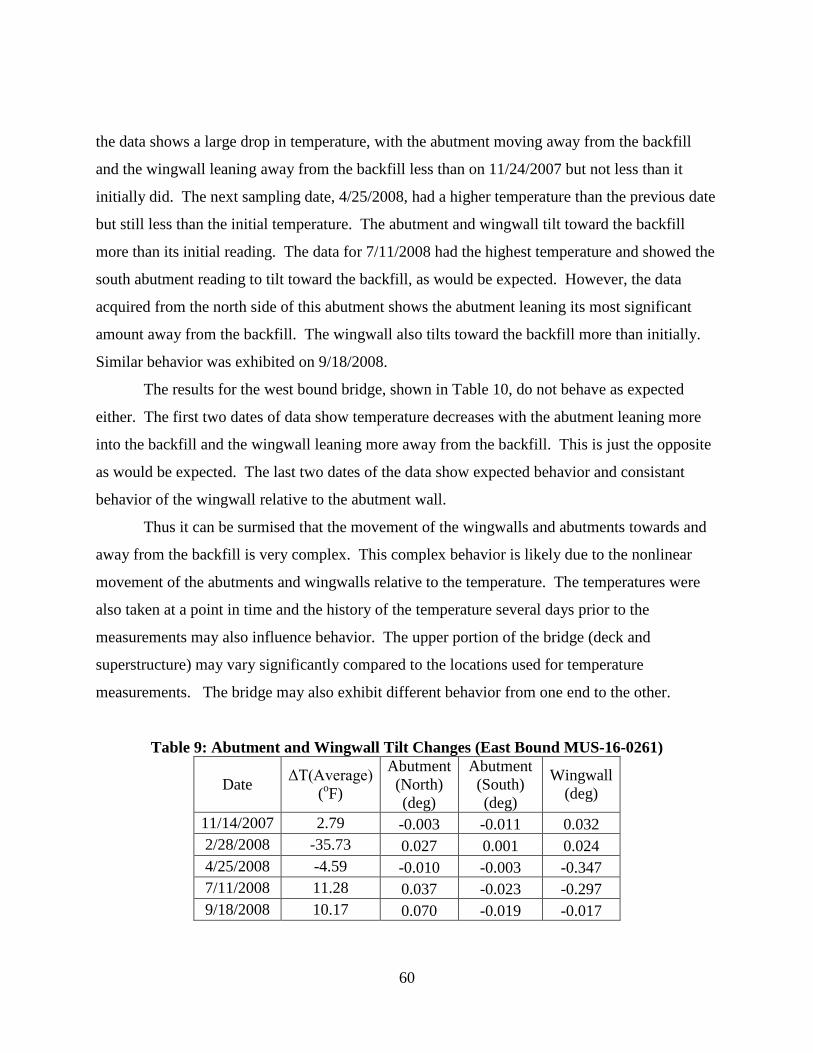
60
the data shows a large drop in temperature, with the abutment moving away from the backfill
and the wingwall leaning away from the backfill less than on 11/24/2007 but not less than it
initially did. The next sampling date, 4/25/2008, had a higher temperature than the previous date
but still less than the initial temperature. The abutment and wingwall tilt toward the backfill
more than its initial reading. The data for 7/11/2008 had the highest temperature and showed the
south abutment reading to tilt toward the backfill, as would be expected. However, the data
acquired from the north side of this abutment shows the abutment leaning its most significant
amount away from the backfill. The wingwall also tilts toward the backfill more than initially.
Similar behavior was exhibited on 9/18/2008.
The results for the west bound bridge, shown in Table 10, do not behave as expected
either. The first two dates of data show temperature decreases with the abutment leaning more
into the backfill and the wingwall leaning more away from the backfill. This is just the opposite
as would be expected. The last two dates of the data show expected behavior and consistant
behavior of the wingwall relative to the abutment wall.
Thus it can be surmised that the movement of the wingwalls and abutments towards and
away from the backfill is very complex. This complex behavior is likely due to the nonlinear
movement of the abutments and wingwalls relative to the temperature. The temperatures were
also taken at a point in time and the history of the temperature several days prior to the
measurements may also influence behavior. The upper portion of the bridge (deck and
superstructure) may vary significantly compared to the locations used for temperature
measurements. The bridge may also exhibit different behavior from one end to the other.
Table 9: Abutment and Wingwall Tilt Changes (East Bound MUS-16-0261)
Date ΔT(Average) (oF)
Abutment (North) (deg)
Abutment (South) (deg)
Wingwall (deg)
11/14/2007 2.79 -0.003 -0.011 0.032 2/28/2008 -35.73 0.027 0.001 0.024 4/25/2008 -4.59 -0.010 -0.003 -0.347 7/11/2008 11.28 0.037 -0.023 -0.297 9/18/2008 10.17 0.070 -0.019 -0.017

61
Table 10: Abutment and Wingwall Tilt Changes (West Bound MUS-16-0261)
Date ΔT(Average) (oF)
Abutment (North) (deg)
Abutment (South) (deg)
Wingwall (deg)
11/14/2007 -12.96 -0.387 -0.095 0.294 2/28/2008 -39.78 -0.016 -0.034 0.228 4/25/2008 0.90 -0.391 -0.085 0.052 7/11/2008 10.81 -0.315 -0.085 0.036 9/18/2008 -10.72 0.380 0.011 -0.712
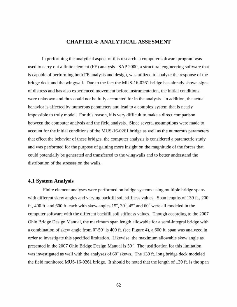
62
CHAPTER 4: ANALYTICAL ASSESMENT
In performing the analytical aspect of this research, a computer software program was
used to carry out a finite element (FE) analysis. SAP 2000, a structural engineering software that
is capable of performing both FE analysis and design, was utilized to analyze the response of the
bridge deck and the wingwall. Due to the fact the MUS-16-0261 bridge has already shown signs
of distress and has also experienced movement before instrumentation, the initial conditions
were unknown and thus could not be fully accounted for in the analysis. In addition, the actual
behavior is affected by numerous parameters and lead to a complex system that is nearly
impossible to truly model. For this reason, it is very difficult to make a direct comparison
between the computer analysis and the field analysis. Since several assumptions were made to
account for the initial conditions of the MUS-16-0261 bridge as well as the numerous parameters
that effect the behavior of these bridges, the computer analysis is considered a parametric study
and was performed for the purpose of gaining more insight on the magnitude of the forces that
could potentially be generated and transferred to the wingwalls and to better understand the
distribution of the stresses on the walls.
4.1 System Analysis Finite element analyses were performed on bridge systems using multiple bridge spans
with different skew angles and varying backfill soil stiffness values. Span lengths of 139 ft., 200
ft., 400 ft. and 600 ft. each with skew angles 15o, 30o, 45o and 60o were all modeled in the
computer software with the different backfill soil stiffness values. Though according to the 2007
Ohio Bridge Design Manual, the maximum span length allowable for a semi-integral bridge with
a combination of skew angle from 0o-50o is 400 ft. (see Figure 4), a 600 ft. span was analyzed in
order to investigate this specified limitation. Likewise, the maximum allowable skew angle as
presented in the 2007 Ohio Bridge Design Manual is 50o. The justification for this limitation
was investigated as well with the analyses of 60o skews. The 139 ft. long bridge deck modeled
the field monitored MUS-16-0261 bridge. It should be noted that the length of 139 ft. is the span

63
length from center to center of the bearing support, and this is true of all the lengths of the
models analyzed.
Several assumptions were made in order to model the deck of the bridge into the FE
software. The entire length of the bridge was modeled for analysis by dividing the deck into
small rhombus shaped thin-shell elements due to the skew (see Figure). The deck shells were
created using a 4.5ksi normal weight (150 pcf) concrete. The value of modulus of elasticity (E)
for the concrete was 3.82 x 10³ ksi as determine using the compressive strength of the concrete
and equation 6 below.
c'f000,57E = (6)
Figure 41: Deck Divided into Rhombus Shell Elements
As explained by MacGregor and Wight (2005), the range of values for poison’s ratio (ν)
of concrete is usually from 0.11 to 0.21 and the coefficient of thermal expansion (α) of normal
weight concrete is from 5 to 7 x 10⁻⁶ strain/oF. MacGregor and Wight (2005) also added that “an
all around value of 5.5 x 10⁻⁶ strain/oF may be used”. Thus, default values of 0.2 and 5.5 x 10⁻⁶
strain/0F were used in the analyses for poison’s ratio and coefficient of thermal expansion,
respectively.
The girder sections for the MUS-16-0261 bridge were grade 50 ASTM A572 welded
steel plate girders, which were created in the program based on the dimensions of the plates
given in the drawings. This was done because the sizes of the girders used in the project were
not available in the software library. According to Metal Suppliers Online, a mean value of
thermal coefficient is 6.7 x 10⁻⁶ strain/oF and an elastic modulus of 30 x 106 psi were used for the
material. In addition, a yield strength value of 50 ksi was used since the material is grade 50.

64
All girder sections were divided into element lengths of the same size as the rhombus thin-shell
elements.
The resistance to motion in the X and Y directions was modeled as linear springs (see
Figure 42). This was done to model the restraining effects on the diaphragms.
Figure 42: Resistance Modeled with Linear Springs
Though the stiffness value for the granular backfill material was not presented in the literature,
stiffness values for sands were assumed (Bowles, 2005). Stiffness values of 35.37 lb/in3, 100.57
lb/in3, and 165.78 lb/in3 were assumed based on similar research conducted by Bettinger (2001).
The wide range of stiffness values investigated could also be thought of as an equivalent stiffness
to take into account the resistance resulting from other sources other than the compression of the
backfill such as the shearing resistance of the bearing pads, the frictional resistance of the
backfill on the superstructure, and the effects of the approach slab. The equivalent stiffness
values were converted into spring stiffness/support (kip/in) in the X and Y directions. The
calculations carried out in converting the stiffness values are presented below. The contact area
(AC) between the diaphragm and backfill was determined by Equation (7). This equation used
the dimensions of the MUS-16-0261 bridge and would vary from bridge to bridge.
×=
×=
)cos(ft33.6ft42
)cos(HWA DD
C θθ (7)
where:
θ = skew angle (degrees)
WD = width of diaphragm
HD = height of diaphragm
The Stiffness/Support was determined from Equation (8).

65
( )
×=
θ cosn ASSSupportStiffness/ C (8)
where:
SS = equivalent stiffness taken as 35.37 lb/in3, 100.57 lb/in3, or 165.78 lb/in3
n = the number of support nodes at the end of the bridge model
A total of nine springs were evenly spaced along the width of diaphragms for all the models with
the exception of 139 ft and 200 ft with a skew angle of 60o. These two models had a total of 17
springs evenly spaced along the width of the abutment. Thus, n = 9 or 17 where appropriate. The
spring stiffness were then broken down into their respective X and Y components using
Equations (9) and (10).
θ cos /Support)(StiffnessXcomp = (9)
θsin /Support)(StiffnessYcomp = (10)
The stiffness values used in the modeling are summarized in Table 11. It should be noted that
the behavior of the resistance is more complex than the assumptions made in order to create the
models for the analyses. However, for the purposes of this research, the simplifying assumptions
made to create the models were adequate to assist in comparing the analyses results with the field
data.
Table 11: Equivalent Stiffness to Spring Stiffness Conversion # of
Springs θ (o)
Equiv. Stiffness (lb/in3)
Ac (ft2)
Stiffness /Support (lb/in3)
Xcomp (lb/in3)
Ycomp (lb/in3)
9 15 35.37 275.24 161.26 155.76 41.74 9 15 100.57 275.24 458.52 442.89 118.67 9 15 165.78 275.24 755.82 730.06 195.62 9 30 35.37 306.99 200.61 173.73 100.30 9 30 100.57 306.99 570.40 493.98 285.20 9 30 165.78 306.99 940.25 814.28 470.13 9 45 35.37 375.98 300.91 212.78 212.78 9 45 100.57 375.98 855.60 605.00 605.00 9 45 165.78 375.98 1,410.38 997.29 997.29 9 60 35.37 531.72 601.82 300.91 521.19 9 60 100.57 531.72 1,711.20 855.60 1.481.94 9 60 165.78 531.72 2,820.75 1,410.38 2,442.84 17 60 35.37 531.72 318.61 159.31 275.93

66
17 60 100.57 531.72 905.93 452.97 784.56 17 60 165.78 531.72 1,493.34 746.67 1,293.27
The 2 in. thick preformed expansion joint filler (PEJF) used between the
wingwall/abutment interface was also modeled as a linear spring at the acute corners of the
bridge model. To determine the stiffness of that spring, compression testing was performed by
Ohio University on the PEJF. The results of the testing are presented in Table 12. The test
required that the PEJF material be able to support a 250 psi compressive stress at 50%
compression deformation of the material. The PEJF test sample size was 4 in. x 4 in. and thus
had an area of 16 in2. The differences in the two tests shown in Table 12 was that the Test 1
samples were tested at laboratory temperature and the Test 2 samples were tested at 95 oF. This
also required the use of two different compression machines. As can be seen in Table 12, the
temperature did not affect the behavior of the PEJF.
The results of Table 12 were determined using abutment/wingwall interface dimensions
of the MUS-16-0261 bridges. The wingwall/diaphragm interface area for the east and west
bound MUS-16-0261 bridges were 2,734.56 in.2 and 3,283.2 in.2, respectively. As can be seen
from Table 12, the average magnitude of force required to compress the PEJF by 1 in. for the
east and west bound MUS-16-0261 bridges were 709 kips and 851 kips, respectively. The stress
associated with these forces as determined in the testing was 259 psi. Since this stress exceeds
the maximum required stress of 250psi in the PEJF, the forces at each wingwall required to
compress the PEJF by 1 in. were back calculated using a compressive stress of 250 psi at the
abutment/wingwall interface. Spring stiffness values at the acute corners of the east and west
bound MUS-16-0261 bridges were thus determined to be 685 kip/in and 820 kip/in, respectively.
These values of 685 kip/in and 820 kip/in were used instead of 709 kip/in and 851 kip/in because
they represent the maximum stress value of 250 psi in the PEJF. In addition 685 kip/in and
820kip/in are conservative values since based on the test, the material can withstand 259 psi of
stress, but the value was reduced to 250 psi.

67
Table 12: PEJF Test Results
Test 1 Results
Initial Thickness
(in)
Thickness After 10 min.
Recovery Period (in)
Load Required to Compress to
50% of Thickness (lbs)
PEJF Stresses
(psi)
Forces at East
Wingwall (kips)
Forces at West
Wingwall (kips)
1.022 0.854 3925 245 671 805 1.034 0.868 3985 249 681 818 1.008 0.846 4417 276 755 907 1.032 0.864 3996 250 683 820 2.078 1.724 4407 275 753 904 2.054 1.678 4528 283 774 929
Average = 4146 259 709 851 Test 2 Results
1.015 0.805 4552 285 778 934 1.002 0.812 4405 275 753 904 1.031 0.867 3492 218 597 717
Average = 4150 259 709 852
The supports at the approach ends of the decks were modeled as rollers to allow for
thermal expansion and contraction. According section 3.12.2 of the Ohio Bridge Design
Manual, a base construction temperature of 60oF shall be assumed for design purposes. A 60oF
temperature change was imparted on the deck and girders of the bridge models assuming bridge
temperatures would not exceed 120oF.
The results of the FEM analyses carried out on the bridge models are presented in
Tables 13 and 14 for the east and west wingwalls, respectively. As shown by the data in
the Tables, the stress in the wingwall only exceeds 250 psi at long spans with high skews
for the assumed soil stiffness values.
Table 13: Forces and Stresses in East Wingwall
Equivalent Stiffness (lb/in3)
Equivalent Stiffness (lb/in3)
35.37 100.57 165.75 35.37 100.57 165.75
Skew Length East Wingwall Forces East Wingwall Stresses

68
(ft) (kips) (psi)
15o
139 58 96 125 21 35 46 200 63 105 138 23 38 50 400 77 134 180 28 49 66 600 92 164 222 34 60 81
30o
139 99 159 205 36 58 75 200 117 188 243 43 69 89 400 173 275 348 63 101 127 600 226 348 429 83 127 157
45o
139 190 253 312 69 93 114 200 216 308 374 79 113 137 400 338 454 525 124 166 192 600 443 351 623 162 205 228
60o
139 214 251 280 78 92 103 200 263 300 413 96 110 151 400 478 584 645 175 214 236 600 616 693 734 225 254 268
Table 14: Forces and Stresses in West Wingwall Equivalent Stiffness
(lb/in3) Equivalent Stiffness
(lb/in3)
35.37 100.57 165.75 35.37 100.57 165.75
Skew Length (ft)
West Wingwall Forces (kips)
West Wingwall Stresses (psi)
15o
139 63 103 132 19 31 40 200 63 106 139 19 32 42 400 83 142 188 25 43 57 600 98 173 230 30 53 70
30o
139 107 170 215 33 52 66 200 126 200 255 38 61 78 400 186 291 363 57 89 110 600 242 368 446 74 112 136
45o 139 176 270 328 53 82 100 200 234 327 392 71 100 119 400 365 482 550 111 147 167

69
600 478 583 651 146 178 198
60o
139 236 272 300 72 83 91 200 289 326 427 88 99 130 400 527 618 672 160 188 205 600 666 732 764 203 223 233
Plots were generated as shown in
Figure Figures 43 - 45 to investigate the effect of varying the length of superstructure, the
skew angle, and the equivalent stiffness on the wingwall stresses for different skews. The
difference in Figures 43 - 45 is the assumed equivalent stiffness.
0
50
100
150
200
250
50 150 250 350 450 550 650
Win
gwal
l Str
ess
(ksi
)
Span Length (ft)
15 deg
30 deg
45 deg
60 deg

70
Figure 43: Span Length on Stresses for Different Skews (kEq = 35.7lb/in3)
Figure 44: Span Length vs Stresses for Different Skews (kEq = 100.57lb/in3)
0
50
100
150
200
250
50 150 250 350 450 550 650
Win
gwal
l Str
ess
(ksi
)
Span Length (ft)
15 deg
30 deg
45 deg
60 deg
0
50
100
150
200
250
300
50 150 250 350 450 550 650
Win
gwal
l Str
ess
(ksi
)
Span Length (ft)
15 deg
30 deg
45 deg
60 deg

71
Figure 45: Span Length vs Stresses for Different Skews (kEq = 165.75 lb/in3)
From Figures 43-45, the higher equivalent stiffness produces a higher stress but
the difference in magnitudes is not that significant for the range of values investigated.
The majority of models investigated showed a range within 50 psi for the skews and
spans modeled.
The longer spans produce larger stresses and the effect becomes more
pronounced for the higher skews. At the skew of 15o, stresses increased less than 50 psi
for the range of spans investigated. However at a 45o skew, the stresses increased over
100 psi for the span range analyzed.
The skew has affects the stresses significantly when the spans are long. Even at
spans of 139 to 200 feet, the stresses increase b 80 psi from 15o to 45o. At the longer 400
and 600 foot spans the stresses increase by well over 100 psi for the 15 o to 45o skews.
Table 15 provides the movement at the abutment wall-wingwall interface for the
model with the 45o skew and the span of 139 ft. The values of the analytical study can be
compared to the results of the field study shown in Tables 3 and 5. The largest joint
displacements measured in the field were approximately 0.22 in. with a 37 oF temperature
0
50
100
150
200
250
300
50 150 250 350 450 550 650
Win
gwal
l Str
ess
(ksi
)
Span Length (ft)
15 deg
30 deg
45 deg
60 deg

72
change. The analytical results show similar magnitude wall joint movements for the
models with the 60oF temperature change leading to some justification of the assumed
equivalent stiffness values assumed. The lower equivalent stiffness of 35.37 lb/in3 show
slightly higher movements and may be more representative of the actual field
instrumented bridge, MUS-16-0261. Differences in the joint movements can also be
attributed to instrumentation being installed well after the bridge was constructed and
experienced numerous daily and seasonal thermal cycles.
Table 25: Analytical Wall Joint Movement (45o skew and Span = 139 ft.)
Equivalent
Stiffness
(lb/in3)
East Joint
Movement
(in)
West Joint
Movement
(in)
35.37 0.249 0.242
100.57 0.223 0.219
165.75 0.204 0.203
4.2 Wingwall and Wall Abutment Interface
A FE model of the wingwall and wall abutment was created by utilizing SAP 2000 (see
Figure 46). The analysis was carried out to investigate the magnitude and stress distribution
pattern at the abutment/wingwall interface and on the surface of the wingwall and wall abutment.
The wingwall and wall abutment model was broken into 1,728 solid elements and the base
support of the walls was assumed fixed. The solid elements were created using a 4.5 ksi normal
weight concrete (150pcf) as given in the project drawings. As aforementioned, the value of
modulus of elasticity (E) used was 3.82 x 10³ ksi.

73
Figure 46: Wingwall and Wall Abutment Model
Only 9 ft. of both the wingwall and wall abutment lengths were modeled. This was done
since the primary interest was the interface between the walls and to reduce the model size along
with the associated computing time of the analysis. A poison’s ratio (ν) and coefficient of
thermal expansion (α) values of 0.2 and 5.5 X 10⁻⁶ strain/oF, respectively (MacGregor and
Wight, 2005) were used.
The loads considered during this analyses included the self weight of both the wingwall
and wall abutment, the dead weight of the deck and girders supported by each abutment, the
lateral earth pressure from the backfill acting on both the wingwall and wall abutment and a 100
psi pressure from the diaphragm acting on the wingwall at the abutment/wingwall interface.
Wall Abutment
Wingwall

74
The following equations were used to calculate the lateral earth pressure of the backfill
against the wingwall and wall abutment (Budhu, 2008). Rankine’s theory of active earth
pressure was used. This is because the passive case (wall pushing against soil) is an extreme
situation and unlikely to be the mode in this case. Passive case is possible when the deck expands
at higher temperatures. Figure47 shows a diagram of the wall and embankment backfill soil.
Equation 11 was used to calculate the active earth pressure coefficient. KaR was
determined to be 0.337 using values of β = 0, η= 2.9o and an assumed value of φ’ = 30o. The
value of φ’ was assumed within the 28o-33o typical range of φ’ for granular soils (Budhu, 2008).
The value of φa needed to evaluate Equation 11 was determined from Equation 12. KaR of 0.337
was found to be close to the typical values determined from similar parameters (Bowles, 1996).
Figure 47: Wall and Backfill
( )βφβη
ϕφφηβ222
2
sin'sincoscos
cos'sin2'sin1)cos(
−+
−+−= a
aRK (11)
where:
KaR = Rankine’s Active Earth Pressure Coefficient

75
𝜙’ = Internal Friction Angle
ηβφβϕ 2
'sinsinsin 1 +−
= −
a (12)
The pressure was then determined using Equation 13hKP aRsoil ⋅⋅= γ
( with an assumed value of 120 pcf for the soil unit weight, γ. This assumed value for the
unit soil weight was within the 106 pcf – 125 pcf typical range for sands (Bowles, 2005).
hKP aRsoil ⋅⋅= γ (13)
where:
Psoil = Soil pressure at a given height
γ = Unit weight of soil
h = height
The soil pressure acting on the face of each solid element was determined by first
calculating the pressure at the top and bottom of each solid element, and then taking the average
between the two pressures. The difference between the pressure at the top and bottom of each
solid element was small. Thus, the elements were considered small enough to assume that the
pressure distribution within a solid element was constant throughout the element.
The 100 psi pressure at the diaphragm/wingwall interface was selected based on the
majority of field measurements were at or below this value and the analytical assessments of the
bridge systems only exceeded 100 psi at large spans and skews. In addition, the analyses of the
bridge systems were based on an assumed equivalent stiffness resisting the thermal induced
movement as well as a ∆T of 60oF. The PEJF laboratory testing resulted in stresses near 250 psi.
However, this was when the compression of the specimen was at one-half its original thickness
of 2”. Field results did not show compression of the diaphragm/wingwall interface as high as 1”.

76
The model for a portion of the abutment wall and wingwall was analyzed once the
necessary assumptions and restraints were imposed and the application of the
aforementioned loads was completed. Figure 48 shows the deflected shape of the model
at the completion of the analysis.
Figure 48: Wall Abutment and Wingwall Deformation By making reference to the deflected of the structure, it can be seen that the front
side of the wingwall is in compression while the back side is in tension. This is due to the
direction of the applied lateral earth pressure acting on the back side as well as the 100
psi load from the diaphragm. In addition, it can be seen that the top of the wall abutment
Original Position
Wall Abutment
Wingwall
77
deformed downward slightly due to the applied deck self-weight. Also, the front side of
the abutment wall is in compression and backside is in tension due to lateral earth
pressure of the backfill acting on the backside. Figure 49 and 50 show the distribution of
vertical normal stresses on the front side and the backside of the wall panels, respectively.
Figure 49: Front Side Stresses (ksi)
Stress Concentration

78
Figure 50: Backside Stresses (ksi)

79
Figure 51 shows the distribution of horizontal normal stresses on the front side of the
wall panels.
Figure 51: Front side Stresses (ksi)

80
CHAPTER 5: CONCLUSIONS
5.1 DEF -24 -0981
The data from the sensors showed that the average stress in the wingwall increased as the
temperature increased. The magnitude of the stress however was not consistently associated
with a specific temperature. This implies that other factors influence the temperature and stress
relationship. Initially the stress distribution over the height of the wall appeared to be close to
uniform for the lower portion of the wall and to be lower near the top of the wall. However, over
time the stress distribution changed shape with a larger stress existing approximately 5.5’ above
the base of the wall. The stresses near the bridge were in general lower than the stresses further
toward the approach slab. This would tend to support the theory of the diaphragm movement
being related to the rotation of the bridge causing higher compression toward the soil side of the
diaphragm.
The data from measuring the joint opening between the wingwall and diaphragm showed
larger openings at lower temperatures. The largest total change in the joint was over 2 inches. In
general, when the joint gap between the wingwall and diaphragm decreases the magnitude of the
stress increased. However, the actual gap measurement did not directly correlate with a specific
magnitude of stress. The behavior of the gap compared to the stress is likely due to the complex
behavior exhibited at the wingwall/diaphragm interface caused by the thermal changes. The
movement of the bridge’s diaphragm at the interface is a combination of longitudinal sliding,
movement in the direction of the skew into the wingwall, and rotation. All of these movements
are also affected by the temperatures that vary in magnitude, duration, history, and location on
the bridge. Therefore, the complex movement cannot be fully measured with the instrumentation
installed only on the front face the wingwall/diaphragm interface.
The stress determined from the VW strain gages varied over the depth of the wingwall
and in time. However, the majority of average stress measurements did not exceed 150 psi. This
150 psi stress is an extreme loading when considering the construction joint at the base of the
wingwall (see Figure 52). Shear through the wingwall is not an issue, but bending at the base of
the wingwall is a concern even with the #6 reinforcing bars on 12” centers. The tension caused

81
by bending is also on the surface of the wingwall that is not viewable for inspection. It is also
difficult to determine how the stress from the diaphragm distributes along the length of the
wingwall to lessen the effect of the bending. Soil on the outside of the wingwall can also assist
in resisting the moment from the diaphragm.
Figure 52: Wingwall Detail (DEF-24-0981)
5.2 MUS - 16- 0261
The data from the joint gap readings showed that the joint gap reduced under
CJ
#6 @ 12”o.c.
Note: Other reinforcement not shown for clarity.
8’3”
1’6”
3’
1’6”
3’ 6” Drilled shaft

82
higher temperatures and increased upon lower temperatures. The largest total movement
of the joint over the sampling period occurred on the east bound bridge and was over
0.3”. Slight changes in the tilt of the abutment walls and the wingwalls were found but
they were very minimal.
The MUS-16-0261 bridge was constructed long before instrumentation was
installed. Therefore, behavior from the instrumentation can only be discussed from the
time of instrumentation. However, review of the plan details for the bridge provided
some additional information (see Figure 53). The bearing retainer shown in the plan
details to have a 0.25” clearance between the retainer and the plate at the bottom of the
girder. The targets used to measure the eastbound bridge were installed in October and
the largest movement of the joint was an opening of the joint of slightly less than 0.23”.
Closing of the joint was less than 0.13” the following July. If the capacity of the retainer
was exceeded, it would have likely been the result of a bearing failure of the concrete at
the bolt and concrete interface. Figure 54 provides an external view of the location of
the bearing retainer and according to the District Bridge Engineer, the location has been
patched. The spalling of the concrete could have been due to bearing failure of the
concrete, especially considering the small amount of cover from the skew effect.
Corrosion of the anchor bolts is likely occurring by evidence of the staining below the
retainer location on the abutment wall.
Another issue is related to the bending of the wingwall caused by the force from
the diaphragm. The reinforcement to resist the tensile force generated by the bending

83
consists of #5’s at 18”o.c. In addition to the limited reinforcement, the minimum
embedment shown is not sufficient for developing the full capacity of the reinforcement.
Figure 53: Wingwall Detail (MUS-16-0261)
CJ
#5 @ 18”o.c
Note: Other reinforcement not shown for clarity.
6’4”
1’5” min
1’6”
Abutment Wall
Diaphragm Girder
HP8x36
PEJF
Steel Plate
Bearing Retainer
LaminatedBearing Pad
Anchor Bolts (3” projection)

84
Figure 54: Bearing Retainer (MUS-16-0261) The results of the field data collected from both bridges and the analytical study show the
behavior of the diaphragm to be very complex due to the numerous factors influencing the
system.
Bearing Retainer

85
CHAPTER 6: RECOMMENDATIONS Based on the results of the following recommendations are made:
• Wingwalls in skewed semi-integral bridges which are turned back to run
longitudinally with the bridge should account for the bending induced in the
wingwall from stress in the wingwall/diaphragm interface generated by thermal
expansion of the bridge.
• For the design of the wingwalls turned to run nearly parallel with the longitudinal
axis of skewed semi-integral bridges should include a 100 psi loading at the
wingwall/diaphragm interface from the thermal expansion of the bridge.
• Though analytical evaluations show that longer spans and higher skews than
allowed by ODOT’s BDM could be used, additional considerations for larger
movements and stresses generated at the wingwall/diaphragm interface would
need to be considered in designs.
• Vertical reinforcement in the wingwall near the bottom of the diaphragm should
have sufficient embedment above and below to meet development length criteria
of the reinforcement.
• Bearing retainers in diaphragms, if used, should assure adequate cover to avoid
spalling of concrete. This is especially true of bridges with very high skews.
• Internal temperatures in the wingwall of the bridge can vary from ambient
temperatures, making it difficult to estimate the affects of the thermal expansion
of the bridge.
• The behavior of the wingwall/diaphragm interface is complex due to the
combination of longitudinal sliding, movement in the direction of the skew into
the wingwall, and rotation. All of these movements are also affected by the
temperatures that vary in magnitude, duration, history, and location on the bridge.
• The construction process, such as the placement of the deck and diaphragm, likely
affects the wingwall/diaphragm interface behavior. Placement during high
temperatures would initially reduce thermal expansion stresses.

86
CHAPTER 7: REFERENCES
Bettinger, C.L. (2001), “Effects of Thermal Expansion on a Skewed Semi-integral Bridge,” A thesis submitted in partial fulfillment of the requirements for the degree of Master of Science, Department of Civil Engineering, Ohio University, Athens, Ohio.
Bowles, J.E. (1996), Foundation Analysis and Design, 5th Ed., McGraw-Hill, New York.
Bridge Design Manual. (2000). Ohio Department of Transportation, Office of Structural Engineering, Columbus, Ohio.
Bridge Design Manual. (2007). Ohio Department of Transportation, Office of Structural Engineering, Columbus, Ohio.
Budhu, M. (2008), Foundations and Earth Retaining Structures, John Wiley and Sons, Ltd, Chichester, West Sussex, United Kingdom.
Burke, M.P., Jr., (2009), Integral and Semi-Integral Bridges, Wiley-Blackwell, John Wiley & Sons, Ltd, Chichester, West Sussex, United Kingdom. Burke, M.P., Jr., and Gloyd, S. (1996). “Semi-integral bridges: A revelation,” Paper presented at The Transportation Research Board’s 75th annual meeting, Washington, D.C., January. Burke, M.P., Jr., (1994A), “Semi-integral Bridges: Movements and Forces,” Transportation Research Record 1460, Transportation Research Board, Washington, D.C., 1-7.
Burke, M.P. (1994B), “The Longitudinal, Lateral and Rotational Movement of Semi-integral Bridges,” Paper presented at The Transportation Research Board’s 73rd annual meeting, Washington, D.C., January.
MacGregor, J.G., and Wight, J.K., (2005), Reinforced Concrete Mechanics and Design, 4th edition, Pearson Prentice Hall, Upper Saddle River, NJ.
Masada, T. (2007). Monitoring of bridge abutment walls at state route 33 over East State Street. Athens, OH. Department of Civil Engineering, Ohio University, Athens, Ohio.
Metal Suppliers Online (2008). “Material property data.”
< http://www.suppliersonline.com> (Feb. 11th, 2008) Metzger, A.T. (1995). Measurement of the abutment forces of a skewed semi-integral bridge as a result of ambient temperature change. Master’s Thesis, Department of Civil Engineering, Ohio University, Athens, Ohio.

87
Omega Engineering Inc. (2007). Omega temperature measurement handbook, 6th Ed., Omega Engineering Inc., Stamford.
Sargand, S. M., Masada, T., and Engle, R. (1999). “Spread footing foundation for highway bridge applications.” Journal of Geotechnical and Geoenvironmental Engineering, 373-382.
Shehu, J., (2009), “Evaluation of the Foundation and Wingwalls of Skewed Semi-Integral Bridges with Wall Abutments,” A thesis submitted in partial fulfillment of the requirements for the degree of Master of Science, Department of Civil Engineering, Ohio University, Athens, Ohio.
Steinberg, E.P., Sargand, S.M., and Bettinger, C.L. (2004), “Forces in Wingwalls of Skewed Semi-Integral Bridges,” Journal of Bridge Engineering, ASCE, Nov/Dec, pp. 563-571.
Steinberg, E.P. and Sargand, S.M., (2001), “Forces Exerted in the Wingwalls of Skewed Semi-Integral Bridges,” Final Report submitted to the U.S. Department of Transportation, Federal Highway Administration and the Ohio Dept. of Transportation, Ohio Research and Transportation Institute (ORITE), Department of Civil Engineering, Ohio University, Athens, Ohio.