food prices pass-through in slovenia - microsoft€¦ · · 2017-08-24food prices pass-through in...
TRANSCRIPT
PRIKAZI IN ANALIZE 5/2012
FOOD PRICES PASS-THROUGH IN SLOVENIA Mateja Gabrijelčič Andreja Lenarčič Mark Pisanski
Izdaja BANKA SLOVENIJE
Slovenska 35
1505 Ljubljana
telefon: 01/ 47 19 000
fax: 01/ 25 15 516
Zbirko PRIKAZI IN ANALIZE pripravlja in ureja Analitsko-raziskovalni center Banke Slovenije
(telefon: 01/ 47 19 680, fax: 01/ 47 19 726, e-mail: [email protected]).
Mnenja in zaključki, objavljeni v prispevkih v tej publikaciji, ne odražajo nujno uradnih stališč Banke Slovenije ali njenih
organov.
http://www.bsi.si/iskalniki/raziskave.asp?MapaId=234
Uporaba in objava podatkov in delov besedila je dovoljena z navedbo vira.
Številka 5, Letnik XVIII
ISSN 1581-2316
FOOD PRICES PASS-THROUGH IN SLOVENIA
Mateja Gabrijelčič, Andreja Lenarčič and Mark Pisanski*
ABSTRACT In light of the recent food commodity price shock, this paper presents a framework for assessing the extent of pass-through of food commodity prices to the two food components in the HICP. It is using a simple bivariate VAR where commodity prices are added as an exogenous variable. In addition to international food commodity prices, newly available series of farm-gate food prices at the euro area and national level constructed by the European Commission's DG-AGRI and ECB are used. The results indicate that using the euro area level DG-AGRI prices is best suited for simulation and forecasting purposes of the Slovenian food prices. A 10% permanent shock in the DG-AGRI euro area prices adds up to 0.4 p.p. to the annual growth of the overall HICP in the first year and up to 0.2 p.p. in the second year. A counterfactual exercise shows that a much larger share of the annual growth rates of Slovenian food prices in 2010/11 can be explained by the shock in foreign food commodity prices than in 2007/08. This is consistent with the view, that a large part of the Slovenian food price inflation in 2007/08 was due to domestic factors, in particular the domestic demand surge, also responsible for most of the rise in the overall HICP at that time.
POVZETEK V kontekstu nedavnega cenovnega šoka na trgu prehranskih surovin, predstavlja to gradivo okvir za ocenjevanje velikosti prenosa cen prehranskih surovin v dve komponenti hrane v HICP. Uporabljena je enostavna vektorska avtoregresija (VAR), pri čemer so cene surovin dodane kot eksogena spremenljivka. Poleg cen prehranskih surovin na mednarodnih trgih, so uporabljene tudi nove časovne serije cen hrane pri kmetijskih proizvajalcih v evrskem območju in v Sloveniji, sestavljene s strani DG-AGRI Evropske komisije in ECB. Rezultati nakazujejo, da je za simulacijo in napovedovanje cen hrane v Sloveniji najbolj primerna serija cen DG-AGRI za evrsko območje. Trajni dvig cen DG-AGRI v evrskem območju za 10% poviša medletno rast slovenskega HICP za 0,4 odstotne točke v prvem letu in za 0,2 odstotne točke v drugem letu po šoku. Simulacije modela kažejo, da je bil delež rasti cen hrane v Sloveniji, ki je pojasnjen s šokom v cenah prehranskih surovin, večji v letih 2010/11, kot v letih 2007/08. To je skladno z dejstvom, da je bil velik del rasti cen hrane v Sloveniji v letih 2007/08 posledica domačih dejavnikov, predvsem rasti domačega povpraševanja, ki je bila tudi razlog za večino rasti skupnega HICP v tistem obdobju.
* All Analysis and Research Department, Bank of Slovenia. E-mail: [email protected], [email protected], [email protected]
4
1. Introduction
Food price shocks on world markets are an important driver of Slovenian inflation, since Slovenia heavily
depends on imports of food commodities, especially soy, sugar and wheat. As food represents over one-fifth of
the Slovenian consumption basket, food prices have been one of the key reasons for rises and falls in headline
inflation in recent years. Developments in the global food markets in recent years demand for greater insight into
the transmission of food shocks into producer prices and final prices for consumers. Therefore, improving the
understanding of the dynamic relationship between commodity prices and final consumer prices has important
benefits for analysing and forecasting inflation.
Since 2006 we have witnessed two international food price shocks and the third shock is currently underway.
Increasing prices of food commodities are raising fears that the food crisis in the years 2007/08 could be
repeated. The rise in food commodity prices on international markets is expected to pass through to producer and
consumer prices, with the magnitude and speed of transmission depending among other on the margins in the
food processing sector and/or in the distribution sector. As the international food price shocks may have far
reaching effects on consumer price inflation, it is essential in respect of the inflation outlook to monitor their
developments and drivers, as well as proper functioning of related markets.
The objective of this note is to analyse the size of pass-through of changes in food commodity prices into
Slovenian food HICP. In addition to the international food price indexes, recently a new database for food prices
in the euro area has become available in the ECB Statistical Data Warehouse (SDW). The database is produced
by the European Commission (DG-AGRI) and improved by the ECB DG Statistics. These data take into account
farm gate and internal market prices and thus implicitly include the effects of the Common Agricultural Policy
(CAP) on food commodity prices. For this reason these series are expected to be more useful for forecasting food
inflation than the international food commodity indices. The DG-AGRI prices are supplied at the national and EU
level.
To asses the size of pass-through of changes in food commodity prices we use a simple reduced form bivariate
vector autoregression (VAR) model. We include the HICP food index and the food component of PPI as
endogenous variables, where the first is divided between unprocessed food and processed food excluding
tobacco and for the latter we take into account Slovenian and the euro area PPI. Food commodity prices and a
12-month moving average of the nominal average net wage growth are included in the model as exogenous
variables. Food commodity prices include either the international food commodity index or DG-AGRI prices at
Slovenian or euro area (EA) level. For robustness, we also consider a simple VAR model. Using Akaike and
Schwarz information criteria we find that the model with EA PPI and with EA DG-AGRI prices fits the data best.
Furthermore, the number of lags suggested by the information criteria varies across the different models and
HICP food subcategories.
The results suggest that a 10 % parallel shift in the DG-AGRI EA prices adds up to 0.4 p.p. to the annual growth
of the overall HICP in the first year and up to 0.2 p.p. in the second year. In comparison with the shocks in DG-
AGRI EA prices, the shocks in DG-AGRI prices at the national level and international commodity index have a
smaller effect on the HICP. According to model simulations the effect of shock on annual inflation dies out after
two years irrespective of the type of commodity index used in the model estimation.
We also conduct a counterfactual exercise, where we consider the assumption of zero growth of food prices in
the international markets from January 2006 for the two sub-indices. We find that the food price shock in 2007/08
5
only partially explains the high y-o-y growth rates of the food price index in Slovenia, while in 2010/2011 the share
of explained y-o-y growth rates of food price index in Slovenia is much larger. The difference is due to several
factors which strongly depend on the state of the domestic demand-driven business cycle.
The rest of the note is organized as follows. The next section analyses the response of food prices in Slovenia to
the shocks on international food prices. Sections 3 and 4 describe the data and the methodology, respectively.
Section 5 presents main results. Section 6 discusses the implication of the analysis for food price boom in
2007/08 and 2010/11 given the assumption of zero annual growth rates of food prices in the international
markets. The last section concludes.
2. The response of Slovenian food prices to the shocks in international food prices
Food prices are, together with energy prices, one of the most volatile components of HICP. As in the case of
energy prices, this volatility reflects to a large extent the influence of commodity prices. In this respect, an
important issue is which food commodity prices should be used as explanatory variables of HICP food inflation.
For Slovenia, the (farm gate) prices determined in the EU may have more explanatory power then food
commodity prices determined in international markets due to the characteristics of internal market driven by EU
Common Agricultural Policy.
Developments in food commodity prices
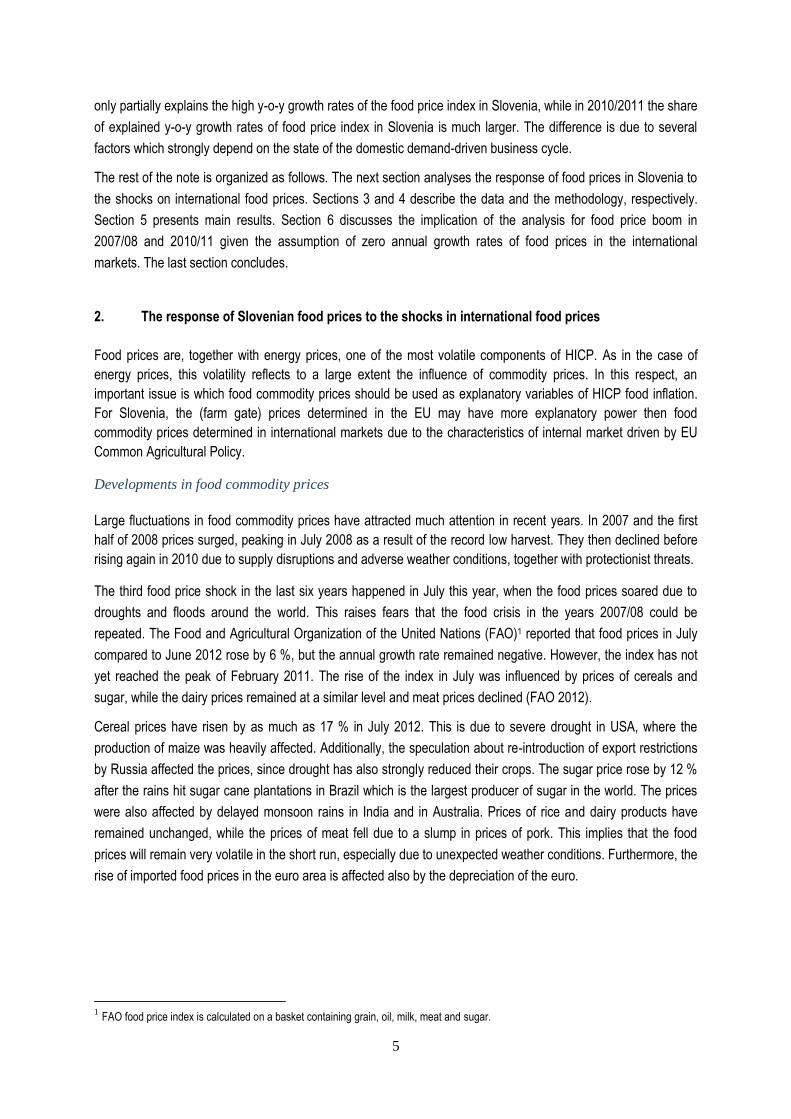
Large fluctuations in food commodity prices have attracted much attention in recent years. In 2007 and the first
half of 2008 prices surged, peaking in July 2008 as a result of the record low harvest. They then declined before
rising again in 2010 due to supply disruptions and adverse weather conditions, together with protectionist threats.
The third food price shock in the last six years happened in July this year, when the food prices soared due to
droughts and floods around the world. This raises fears that the food crisis in the years 2007/08 could be
repeated. The Food and Agricultural Organization of the United Nations (FAO)1 reported that food prices in July
compared to June 2012 rose by 6 %, but the annual growth rate remained negative. However, the index has not
yet reached the peak of February 2011. The rise of the index in July was influenced by prices of cereals and
sugar, while the dairy prices remained at a similar level and meat prices declined (FAO 2012).
Cereal prices have risen by as much as 17 % in July 2012. This is due to severe drought in USA, where the
production of maize was heavily affected. Additionally, the speculation about re-introduction of export restrictions
by Russia affected the prices, since drought has also strongly reduced their crops. The sugar price rose by 12 %
after the rains hit sugar cane plantations in Brazil which is the largest producer of sugar in the world. The prices
were also affected by delayed monsoon rains in India and in Australia. Prices of rice and dairy products have
remained unchanged, while the prices of meat fell due to a slump in prices of pork. This implies that the food
prices will remain very volatile in the short run, especially due to unexpected weather conditions. Furthermore, the
rise of imported food prices in the euro area is affected also by the depreciation of the euro.
1 FAO food price index is calculated on a basket containing grain, oil, milk, meat and sugar.
6
Figure 2.1: Prices of selected agricultural commodities (in USD) - index and y-o-y change
Source: FAO.
Although these price pressures in agricultural commodity markets were driven by idiosyncratic factors, there are
also some common factors affecting medium to long-run demand trends. One factor represents increased
demand stemming from emerging markets due to changes in demography and dietary preferences. Another is
the rise in demand for food crops (in particular sugar and maize) for the production of biofuels. Prices, however,
crucially depend also on the supply-side speed of adjustment. Since agricultural technologies have remained
largely unchanged over the last two decades, this implies that higher yields cannot be obtained without further
improvements. All these factors suggest that there will remain an upside pressure on food prices in the long-run
(ECB Monthly Bulletin, 2009).
Developments in food commodity prices in Slovenia
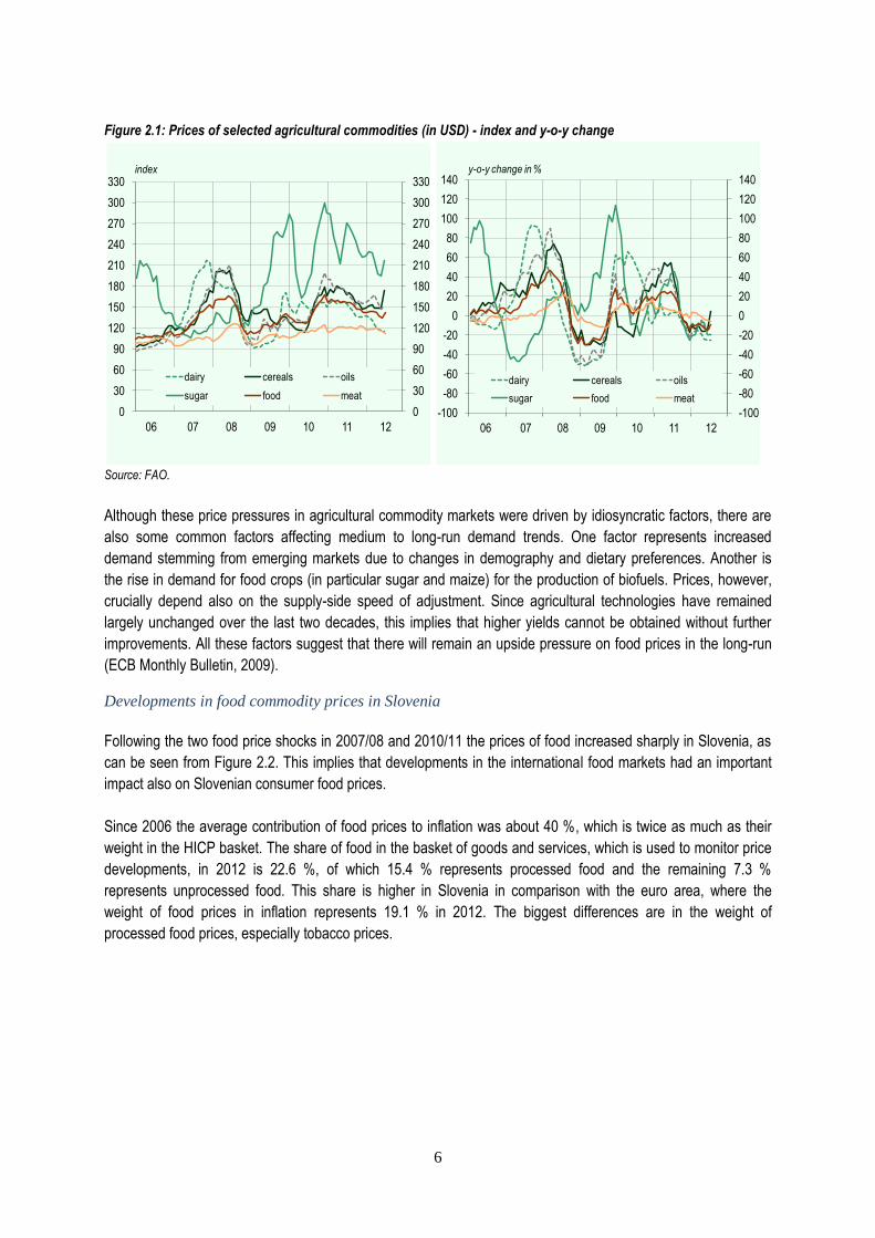
Following the two food price shocks in 2007/08 and 2010/11 the prices of food increased sharply in Slovenia, as
can be seen from Figure 2.2. This implies that developments in the international food markets had an important
impact also on Slovenian consumer food prices.
Since 2006 the average contribution of food prices to inflation was about 40 %, which is twice as much as their
weight in the HICP basket. The share of food in the basket of goods and services, which is used to monitor price
developments, in 2012 is 22.6 %, of which 15.4 % represents processed food and the remaining 7.3 %
represents unprocessed food. This share is higher in Slovenia in comparison with the euro area, where the
weight of food prices in inflation represents 19.1 % in 2012. The biggest differences are in the weight of
processed food prices, especially tobacco prices.
0
30
60
90
120
150
180
210
240
270
300
330
06 07 08 09 10 11 12
0
30
60
90
120
150
180
210
240
270
300
330
dairy cereals oils
sugar food meat
index
-100
-80
-60
-40
-20
0
20
40
60
80
100
120
140
06 07 08 09 10 11 12
-100
-80
-60
-40
-20
0
20
40
60
80
100
120
140
dairy cereals oils
sugar food meat
y-o-y change in %
7
Figure 2.2: Contribution to inflation Figure 2.3: Tobacco prices
Source: Eurostat, Bank of Slovenia calculations.
The average annual increase of food prices in Slovenia since 2006 was 4.4 %, 2.0 p.p. more than on average in
the euro area. The increase in HICP food prices in Slovenia was much higher after the 2007/08 food shock than
in 2010/11. One reason for this is that Slovenian food prices strongly depend on business cycle (see Section 6).
At the peak in the beginning of 2008, high domestic spending and above the long-run average (trend) of
aggregate demand, enabled Slovenian retailers to increase their prices for consumers over-proportionately. In
contrast, due to the crisis, retailers were unable to fully raise prices after the 2010/2011 shock since the
consumer behaviour became more precautionary and their spending decreased due to lower disposable income.
In line with this, it is expected that the current increase in food prices on international markets will be somewhat
offset by lower retailers' margins due to lower consumer purchasing power.
Since 2006 the processed food prices were strongly driven also by increases in prices of tobacco, which
represented 40 % of the contribution of processed food prices to HICP. The rise of tobacco prices was mostly due
to increases in excise duties. Before the crisis, the adjustment of excise duties was set to reach European
tobacco excise duties standards. In May 2009, the government increased excise duties on tobacco as one of the
measures to alleviate the impact of the economic crisis on the State budget. In 2010, the new Excise Duties Act
envisaged six increases in excise duties on tobacco until 2012. This was in line with the European directive by
which all EU Member States must raise excise duties to a minimum of EUR 90 per 1,000 cigarettes by no later
than January 2014. The latest price increase was executed in July 2012 and due to fiscal consolidation needs,
the government also announced additional two increases in the next months. Since tobacco prices are not
subject to the movements in foreign food prices, we excluded them from the processed food price index for the
purposes of our analysis of the pass-through.
3. New database
The new food commodity database is produced by the European Commission's Directorate General for
Agriculture (EU DG-AGRI)2. In comparison with international food prices that we have used for analysis and
forecasts, the Commission's database collects prices of food items observed inside the EU, thereby capturing the
2 For further details, see the data by the European Commission, available at: http://ec.europa.eu/agriculture/markets/prices/monthly_en.pdf
-2
-1
0
1
2
3
4
5
6
7
8
06 07 08 09 10 11 12
-2
-1
0
1
2
3
4
5
6
7
8
services
energy
non-energy industrial goods
processed food
unprocessed food
HICP
y-o-y growth in %; contributions in p.p.
-5
0
5
10
15
20
06 07 08 09 10 11 12
-5
0
5
10
15
20
y-o-y growth in %
8
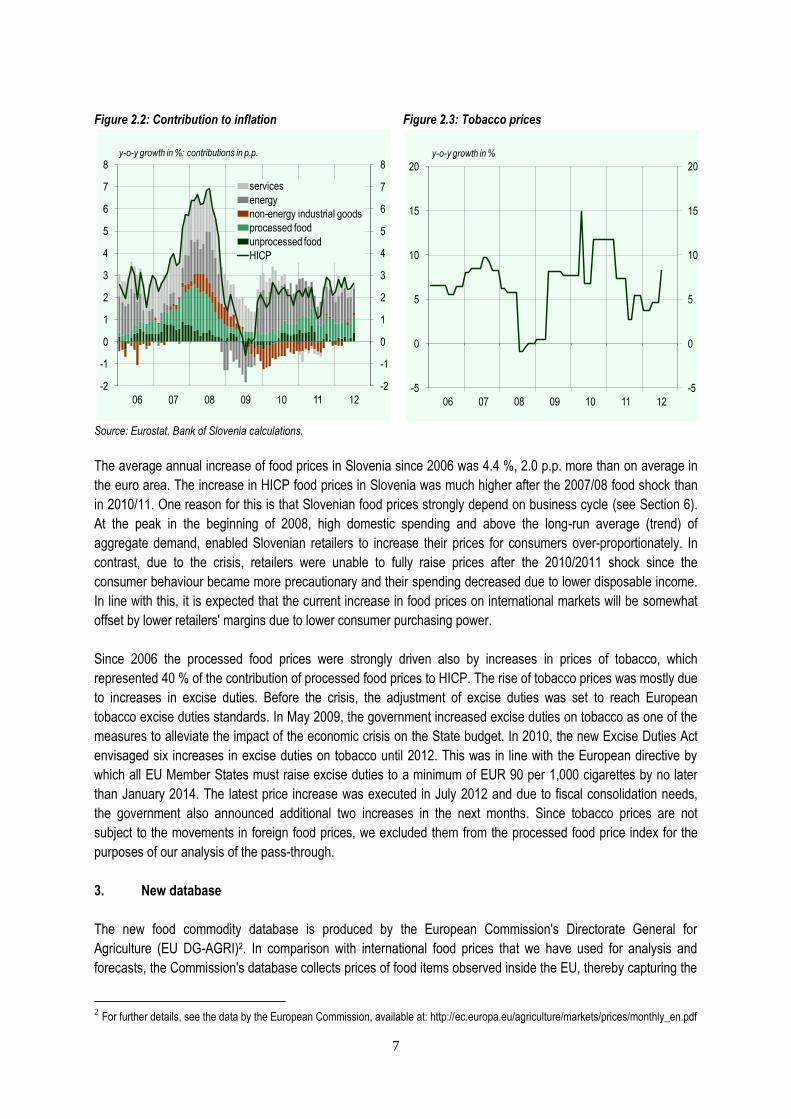
impact of Common Agricultural Policy (CAP). Over the summer of 2011 DG-Statistics in the ECB has improved
the data quality of these price indices and made them available in SDW. The data are available as aggregate
euro area DG-AGRI prices and national DG-AGRI prices. Additionally, the database also contains detailed price
information for several food agricultural commodities produced directly in the EU: cereal (maize, wheat for flour),
meat (beef, calves, chicken, cows, heifers, lamb, pork), oils and butter and dairy (Edam cheese, eggs, milk). One
caveat is that among all products considered in the unprocessed food component, DG-AGRI covers only meat
products.
Figure 3.1: Comparison of international, DG-AGRI and HICP food prices
Source: ECB, European Commission.
The comparison between newly available DG-AGRI prices and international food commodity prices shows that
international commodity prices are much more volatile than DG-AGRI prices, especially prior to 2005. Thereafter
the two indices have become more closely related. Furthermore, the HICP food index (consumer prices) show
higher correlation with both Slovenian DG-AGRI (SI DG-AGRI) and euro area DG-AGRI (EA DG-AGRI) than
international prices, suggesting that the first two may be a better gauge of commodity input cost pressures faced
by the food processing industry and retailers in the euro area.
The first users of the new database were Ferrucci et al. (2010), who compared the pass-through of these prices
with international food commodity price data for the euro area. They use a VAR model and find evidence of a
statistically and economically significant food price pass-through in the euro area when EU DG-AGRI prices are
used. Conversely, they find statistically insignificant pass-through when international commodity prices are used.
From this they conclude that the CAP plays a crucial role in the transmission mechanism of food price shocks in
the euro area.
-30
-20
-10
0
10
20
30
40
50
60
2000 2001 2002 2003 2004 2005 2006 2007 2008 2009 2010 2011 2012
-30
-20
-10
0
10
20
30
40
50
60
international food prices HICP food Slovenia
DG AGRI prices euro area DG AGRI prices Slovenia
Comparison of international, DG AGRI and HICP food prices
y-o-y change in %
9
4. Model
In order to assess the size of the pass-through of changes in food commodity prices on international and
domestic markets to Slovenian food HICP, this relation needs to be formally modelled. To this end, a simple
reduced form bivariate VAR consisting of the HICP food index and the food component of PPI is constructed.3
Since we are interested in estimating the transmission of food price shocks at a more disaggregated level, our
model includes either the unprocessed food price index or the price index for processed food excluding tobacco.4
Additionally, the food commodity prices and a 12-month moving average of the nominal average net wage growth
are added as exogenous explanatory variables.
A general form of the model can be written in the following way:
= , (1)
where includes either the Slovenian or EA food producer price index, and either unprocessed food or
processed food price index excluding tobacco. The ordering of these variables is irrelevant for our exercise, since
we are not interested in the effects that shocks in PPI have on the HICP and vice versa. The vector of
endogenous variables enters the model with lags. Commodity prices are denoted with and include either the
international food commodity index or DG-AGRI prices at Slovenian or EA level. We assume that commodity
prices affect PPI and HICP contemporaneously and with lags, while keeping them exogenous to the VAR. With
the latter we presume that domestic PPI and HICP series have no effect on commodity prices at any time
horizon. While this assumption is warranted in most combinations of the included variables, it is probably a bit too
restrictive in the case when we have Slovenian DG-AGRI prices. We address this issue by estimating also a full
VAR as described in the next paragraph. Next, stands for a twelve month moving average of the average
nominal net wage growth5. By including some measure of income we control for the demand factors that could
drive inflation, which is supposed to improve the fit and forecasting performance of the model. Finally, we include
the euro-tolar exchange rate, denoted as , to correct for the exchange rate changes in the period before the
introduction of euro. All variables except the nominal net wage growth enter the model in log differences and we
use monthly dummies, denoted as to control for seasonal effects. and denote the coefficient
matrices of corresponding sizes.6
In addition to the "baseline" model above, we also estimate a simple VAR where the vector of endogenous
variables includes the food commodity price index (defined as in the baseline model), either the Slovenian
or EA food producer price index , and a food sub-index of interest, denoted as . The ordering of these
variables is in line with the idea that there is no contemporaneous feedback from PPI and HICP to the food
commodity prices and no contemporaneous feedback from HICP to PPI. Structural impulse responses can be
then obtained using Cholesky decomposition. Differently from the baseline model, this model allows for some
delayed feedback from final consumer prices and producer prices to the commodity prices. This would be
plausible when working for instance with Slovenian DG-AGRI series. The vector of endogenous variables enters
3 We include the PPI data following the paper by Ferrucci et al. (2010).
4 We exclude tobacco since tobacco prices change primarily due to the governmental excise policy, as described in Section 2, and have
little if any link to the international food commodity prices. 5 The moving average is calculated using the current month plus past 11 months.
6 Note that due to a two month delay in the availability of the nominal wage data, we need to resort to official Bank of Slovenia wage
forecasts (produced in the framework of BMPE) at a quarterly level and interpolate the data to fill the gap.
10
the model with lags and all variables enter the model in log differences. The only exceptions are, as in the
baseline model, the monthly dummies and a 12-month moving average of the nominal average net wage growth.
Choosing the best specification
In the next step, we calculate the value of Akaike (AIC) and Schwarz (SIC) information criteria for different
variants of the model in order to assess the fit of the model, which gives us an idea about which international food
commodity price index is the most relevant for explaining the movements in the Slovenian food HICP.
Subsequently, we use the same criteria to determine the optimal lag structure. In Annex A, we present the AIC
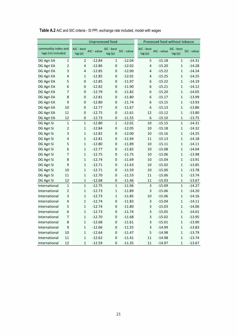
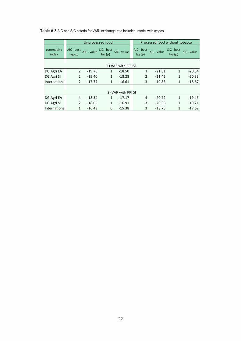
and SIC criteria for the baseline model (Table A.1 with EA PPI and Table A.2 with Slovenian PPI), and values of
information criteria for the alternative "full VAR" model (Table A.3).
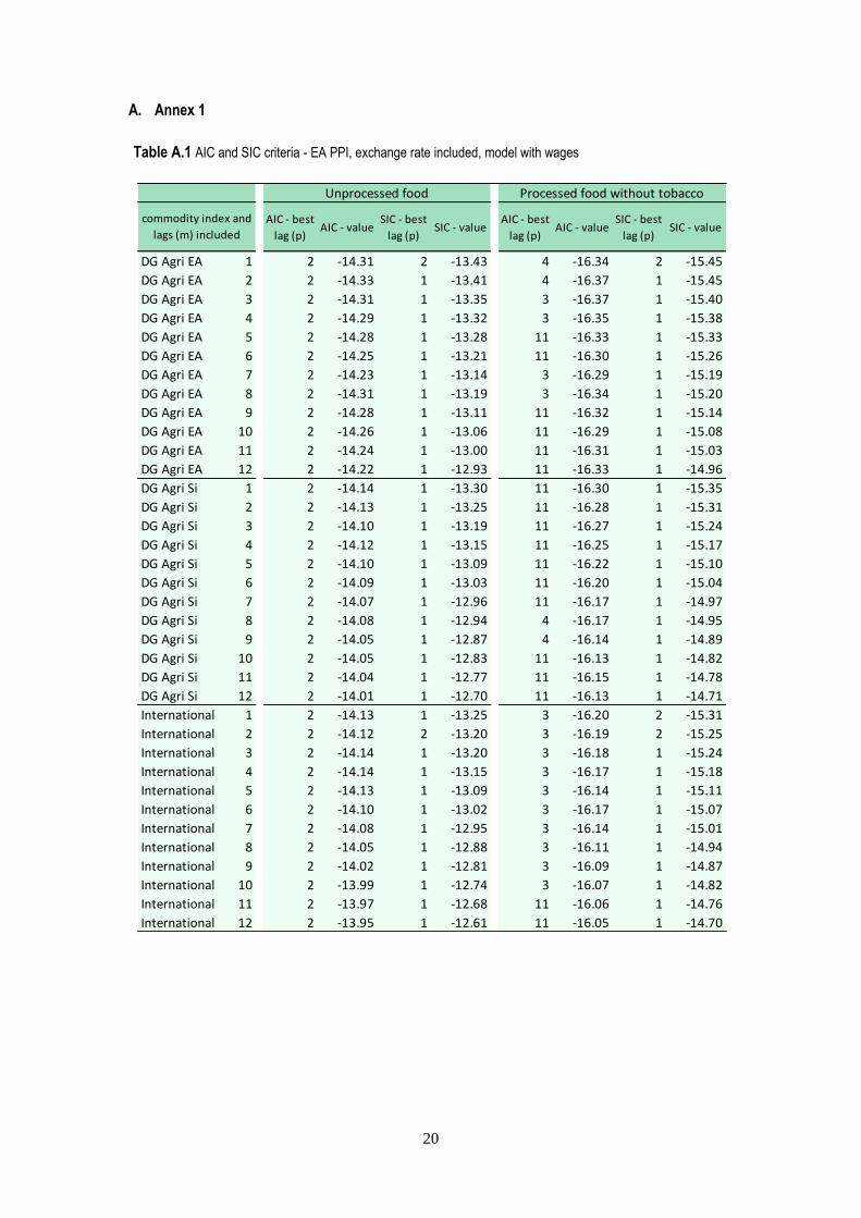
Turning first to the fit of the baseline model, we notice that the model with EA PPI (Table A.1) outperforms the
model with Slovenian PPI (Table A.2), as demonstrated by lower values of information criteria. Next, focusing on
Table A.1 we see that the best fitting model is the one where we use DG-AGRI prices at the EA level. The fit of
the model is thus superior to the fit of models with national level of DG-AGRI prices or international commodity
prices and this result holds for both, the unprocessed food prices and processed food prices excluding tobacco.
Further ranking of the models is less clear-cut as the differences are very small. In the case of unprocessed food
HICP, the model fits the data approximately equally well with Slovenian DG-AGRI prices and with the
international commodity prices, while for the processed food HICP excluding tobacco, the model with Slovenian
DG-AGRI time series slightly outperforms the model with international commodity prices. Very small differences
in the values of information criteria mean that the fit of the model is approximately equally good across such
cases.
Similarly to the results above, the full VAR model fits the data better when using EA PPI, compared to the model
with Slovenian PPI (Table A.3). Moreover, also in this case we find that the model with EA DG-AGRI fits the data
better than the rest, followed by the model with SI DG-AGRI and as third, the model with international food
commodity prices. Given the results above, we focus on models with EA food PPI in the rest of the paper. The
number of lags suggested by the information criteria varies across the different variants of the model and across
the two subcategories of food HICP that we are analysing. We present the summary of chosen lags in Table 4.1.
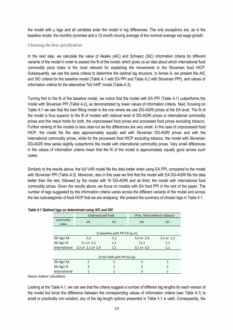
Table 4.1 Optimal lags as determined using AIC and SIC
Source: Authors' calculations.
Looking at the Table 4.1, we can see that the criteria suggest a number of different lag lengths for each version of
the model but since the difference between the corresponding values of information criteria (see Table A.1) is
small or practically non existent, any of the lag length options presented in Table 4.1 is valid. Consequently, the
commodity
indexAIC SIC AIC SIC
DG Agri EA 2,2 2,1 4,2 or 3,3 2,1 or 1,2
DG Agri SI 2,1 or 2,2 1,1 11,1 1,1
International 2,3 or 2,1 or 2,4 1,1 3,1 or 3,2 1,1
DG Agri EA 2 1 3 1
DG Agri SI 2 1 2 1
International 2 1 3 1
Proc. food without tobacco
1) baseline with PPI EA (p,m)
2) full VAR with PPI EA (p)
Unprocessed food
11
rest of the paper presents a range of results suggested by different specifications. Note, however, that several
econometric studies have confirmed (see for instance Hannan (1982), Sneek (1984) and Koehler and Murphree
(1988)), the AIC tends to suggest too many lags and leads to overparametrisation. The SIC criterion is thus seen
as better for choosing the lag length in ARMA (p,q) type of models.
5. Results: the estimate of the food price pass-through
In this section, the results of model simulations of a response of Slovenian food prices to a 10% parallel shift in
the prices of food commodities. For this we use the "baseline" model that contains the optimal number of lags, as
suggested by the results in Section 4. Since we want to compare the strength of the pass-through of shocks in
different commodity indices, while not confounding the results with different number of lags used, we first perform
a baseline simulation where we use p=4 and m=2 lags for processed food excluding tobacco and p=m=2 lags for
the unprocessed food. We perform this exercise using three different food commodity indices: the DG-AGRI index
at EA level, the DG-AGRI index for Slovenia and the international commodity index. Further, we use EA level
food PPI as the series and the coefficients of the model are estimated on the sample running from 2000m1 to
2011m12.
In Table 4.1, we report the estimated effect of the shift in commodity prices on the two price sub-indices,
unprocessed food and processed food excluding tobacco, and on the total food HICP and overall HICP. The
response is expressed in terms of percentage points that a 10% parallel shift would add to the annual (y-o-y)
inflation of the price category of interest. The results are also plotted in Figure 4.1 for easier inspection.
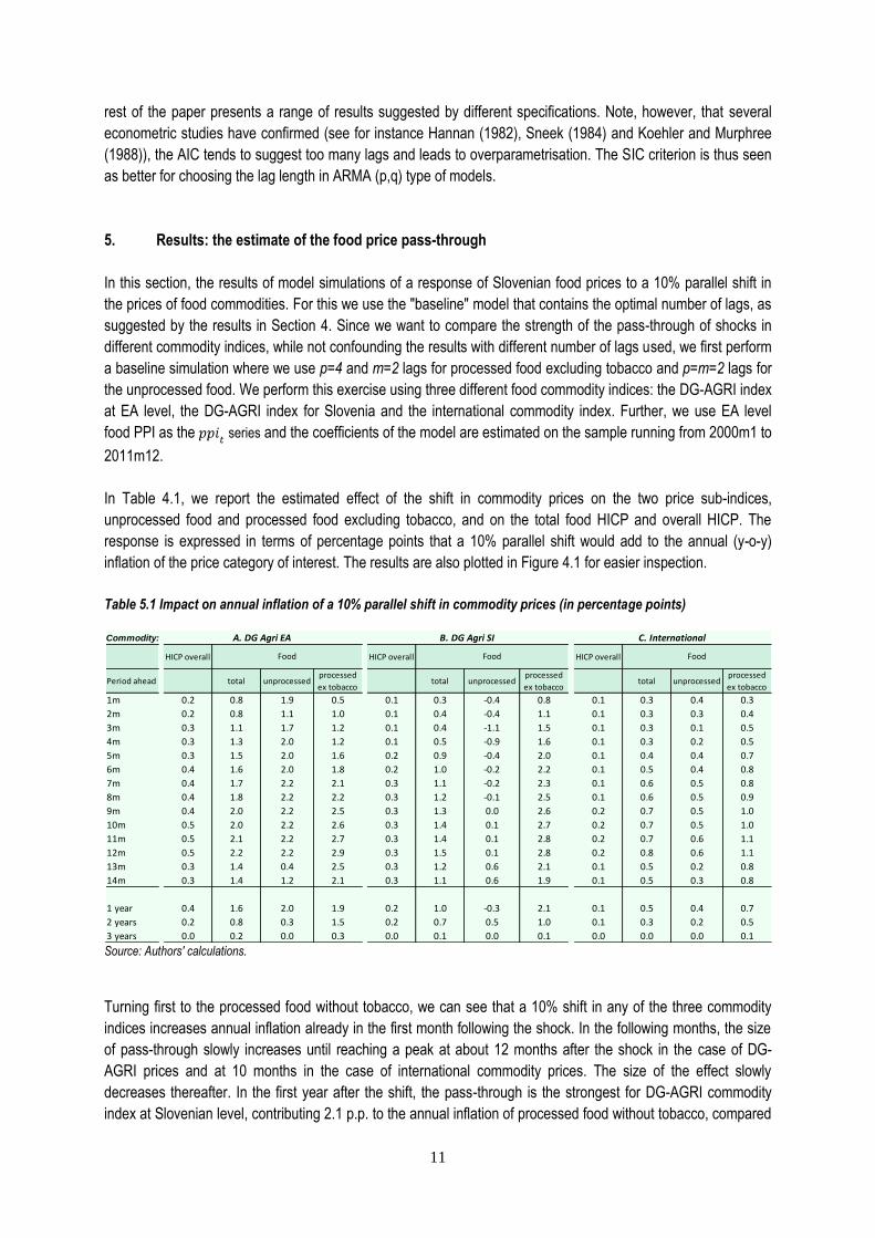
Table 5.1 Impact on annual inflation of a 10% parallel shift in commodity prices (in percentage points)
Source: Authors' calculations.
Turning first to the processed food without tobacco, we can see that a 10% shift in any of the three commodity
indices increases annual inflation already in the first month following the shock. In the following months, the size
of pass-through slowly increases until reaching a peak at about 12 months after the shock in the case of DG-
AGRI prices and at 10 months in the case of international commodity prices. The size of the effect slowly
decreases thereafter. In the first year after the shift, the pass-through is the strongest for DG-AGRI commodity
index at Slovenian level, contributing 2.1 p.p. to the annual inflation of processed food without tobacco, compared
Commodity:
HICP overall HICP overall HICP overall
Period ahead total unprocessedprocessed
ex tobaccototal unprocessed
processed
ex tobaccototal unprocessed
processed
ex tobacco
1m 0.2 0.8 1.9 0.5 0.1 0.3 -0.4 0.8 0.1 0.3 0.4 0.3
2m 0.2 0.8 1.1 1.0 0.1 0.4 -0.4 1.1 0.1 0.3 0.3 0.4
3m 0.3 1.1 1.7 1.2 0.1 0.4 -1.1 1.5 0.1 0.3 0.1 0.5
4m 0.3 1.3 2.0 1.2 0.1 0.5 -0.9 1.6 0.1 0.3 0.2 0.5
5m 0.3 1.5 2.0 1.6 0.2 0.9 -0.4 2.0 0.1 0.4 0.4 0.7
6m 0.4 1.6 2.0 1.8 0.2 1.0 -0.2 2.2 0.1 0.5 0.4 0.8
7m 0.4 1.7 2.2 2.1 0.3 1.1 -0.2 2.3 0.1 0.6 0.5 0.8
8m 0.4 1.8 2.2 2.2 0.3 1.2 -0.1 2.5 0.1 0.6 0.5 0.9
9m 0.4 2.0 2.2 2.5 0.3 1.3 0.0 2.6 0.2 0.7 0.5 1.0
10m 0.5 2.0 2.2 2.6 0.3 1.4 0.1 2.7 0.2 0.7 0.5 1.0
11m 0.5 2.1 2.2 2.7 0.3 1.4 0.1 2.8 0.2 0.7 0.6 1.1
12m 0.5 2.2 2.2 2.9 0.3 1.5 0.1 2.8 0.2 0.8 0.6 1.1
13m 0.3 1.4 0.4 2.5 0.3 1.2 0.6 2.1 0.1 0.5 0.2 0.8
14m 0.3 1.4 1.2 2.1 0.3 1.1 0.6 1.9 0.1 0.5 0.3 0.8
1 year 0.4 1.6 2.0 1.9 0.2 1.0 -0.3 2.1 0.1 0.5 0.4 0.7
2 years 0.2 0.8 0.3 1.5 0.2 0.7 0.5 1.0 0.1 0.3 0.2 0.5
3 years 0.0 0.2 0.0 0.3 0.0 0.1 0.0 0.1 0.0 0.0 0.0 0.1
Food Food Food
A. DG Agri EA B. DG Agri SI C. International
12
to the pass-through of 1.9 p.p. that we observe in the case of EA level commodity prices. Conversely, the pass-
through in the second year is at 1.5 p.p. stronger in the case EA level commodity prices, compared to the 1.0 p.p.
of the pass-through after a shift in the DG-AGRI SI index. The shock of the same size in the international
commodity prices contributes only 0.7 p.p. to the annual growth of the processed food prices without tobacco in
the first year after the shock and 0.5 p.p. in the second year. The effects in the third year after the shock are
estimated to be small.
When looking at the unprocessed food column in Table 4.1, we observe that the size and sign of the response
are quite diverse. The pass-through in the first year is the strongest after a 10% shift in the DG-AGRI EA prices,
where the pass-through is strong already in the first month, reaching the peak of 2.2 p.p. in 7 months after the
shock, and starts to decline after 12 months. The pass-through of a shock in the international commodity price
index is much more subdued and in the first year on average contributes 0.4 p.p. to the annual inflation in
unprocessed food, compared to 2.0 p.p. in the case of DG-AGRI EA. Interestingly, a 10% shift in the Slovenian
DG-AGRI price index is passed through to the unprocessed food prices in a very different fashion. In the first
eight months the shock lowers the annual inflation by 0.5 p.p. on average, while in the following months the effect
is positive.
Note that the response of unprocessed food HICP is subject to some uncertainty. This may be due to high
volatility in the unprocessed food HICP series that can in the context of a rather short sample deliver estimates
that could be somewhat imprecise. Also, the commodity price indices are expected to have difficulties in
improving projections of unprocessed food HICP, since they do not contain any series that could predict the
prices of vegetables and fruit that constitute approximately 40% of unprocessed food HICP and account for most
of the volatility in this index.
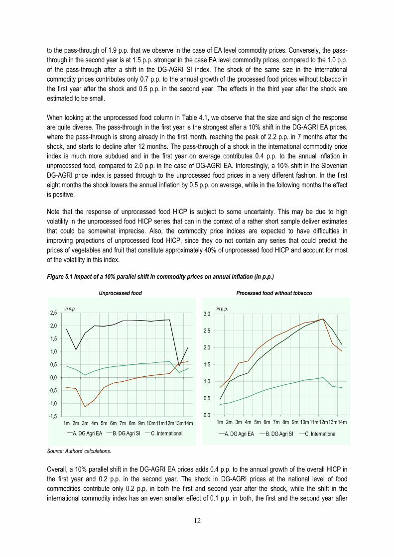
Figure 5.1 Impact of a 10% parallel shift in commodity prices on annual inflation (in p.p.)
Unprocessed food Processed food without tobacco
Source: Authors' calculations.
Overall, a 10% parallel shift in the DG-AGRI EA prices adds 0.4 p.p. to the annual growth of the overall HICP in
the first year and 0.2 p.p. in the second year. The shock in DG-AGRI prices at the national level of food
commodities contribute only 0.2 p.p. in both the first and second year after the shock, while the shift in the
international commodity index has an even smaller effect of 0.1 p.p. in both, the first and the second year after
-1,5
-1,0
-0,5
0,0
0,5
1,0
1,5
2,0
2,5
1m 2m 3m 4m 5m 6m 7m 8m 9m 10m11m12m13m14m
A. DG Agri EA B. DG Agri SI C. International
in p.p.
0,0
0,5
1,0
1,5
2,0
2,5
3,0
1m 2m 3m 4m 5m 6m 7m 8m 9m 10m11m12m13m14m
A. DG Agri EA B. DG Agri SI C. International
in p.p.
13
the shock. After two years the effect of the shock on annual HICP inflation dies out irrespective of the type of
commodity index applied in the simulation.
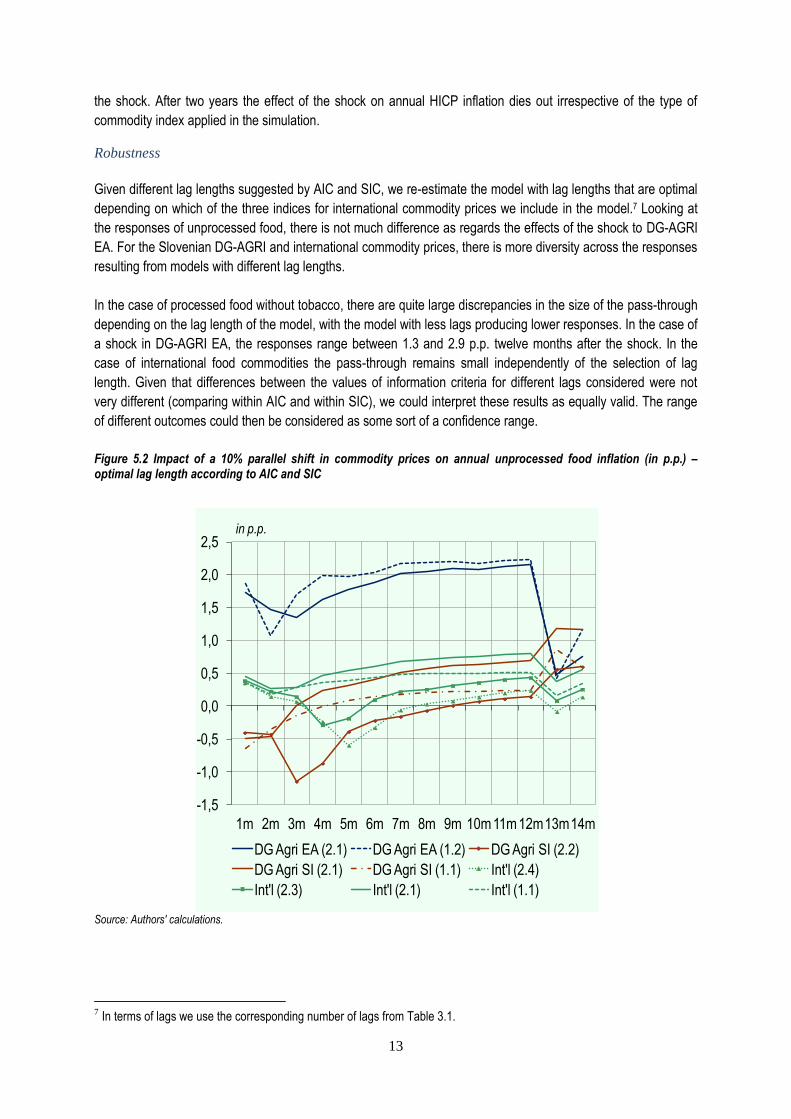
Robustness
Given different lag lengths suggested by AIC and SIC, we re-estimate the model with lag lengths that are optimal
depending on which of the three indices for international commodity prices we include in the model.7 Looking at
the responses of unprocessed food, there is not much difference as regards the effects of the shock to DG-AGRI
EA. For the Slovenian DG-AGRI and international commodity prices, there is more diversity across the responses
resulting from models with different lag lengths.
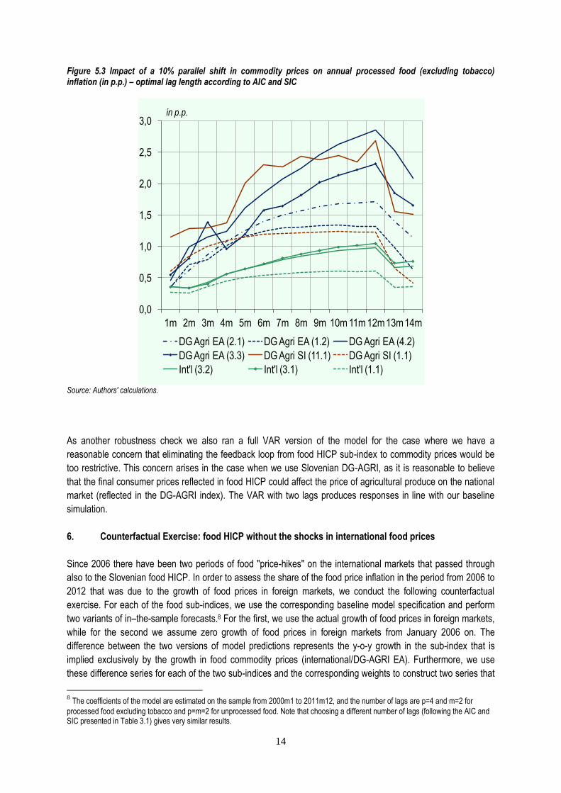
In the case of processed food without tobacco, there are quite large discrepancies in the size of the pass-through
depending on the lag length of the model, with the model with less lags producing lower responses. In the case of
a shock in DG-AGRI EA, the responses range between 1.3 and 2.9 p.p. twelve months after the shock. In the
case of international food commodities the pass-through remains small independently of the selection of lag
length. Given that differences between the values of information criteria for different lags considered were not
very different (comparing within AIC and within SIC), we could interpret these results as equally valid. The range
of different outcomes could then be considered as some sort of a confidence range.
Figure 5.2 Impact of a 10% parallel shift in commodity prices on annual unprocessed food inflation (in p.p.) – optimal lag length according to AIC and SIC
Source: Authors' calculations.
7 In terms of lags we use the corresponding number of lags from Table 3.1.
-1,5
-1,0
-0,5
0,0
0,5
1,0
1,5
2,0
2,5
1m 2m 3m 4m 5m 6m 7m 8m 9m 10m11m12m13m14m
DG Agri EA (2.1) DG Agri EA (1.2) DG Agri SI (2.2)
DG Agri SI (2.1) DG Agri SI (1.1) Int'l (2.4)
Int'l (2.3) Int'l (2.1) Int'l (1.1)
in p.p.
14
Figure 5.3 Impact of a 10% parallel shift in commodity prices on annual processed food (excluding tobacco) inflation (in p.p.) – optimal lag length according to AIC and SIC
Source: Authors' calculations.
As another robustness check we also ran a full VAR version of the model for the case where we have a
reasonable concern that eliminating the feedback loop from food HICP sub-index to commodity prices would be
too restrictive. This concern arises in the case when we use Slovenian DG-AGRI, as it is reasonable to believe
that the final consumer prices reflected in food HICP could affect the price of agricultural produce on the national
market (reflected in the DG-AGRI index). The VAR with two lags produces responses in line with our baseline
simulation.
6. Counterfactual Exercise: food HICP without the shocks in international food prices
Since 2006 there have been two periods of food "price-hikes" on the international markets that passed through
also to the Slovenian food HICP. In order to assess the share of the food price inflation in the period from 2006 to
2012 that was due to the growth of food prices in foreign markets, we conduct the following counterfactual
exercise. For each of the food sub-indices, we use the corresponding baseline model specification and perform
two variants of in–the-sample forecasts.8 For the first, we use the actual growth of food prices in foreign markets,
while for the second we assume zero growth of food prices in foreign markets from January 2006 on. The
difference between the two versions of model predictions represents the y-o-y growth in the sub-index that is
implied exclusively by the growth in food commodity prices (international/DG-AGRI EA). Furthermore, we use
these difference series for each of the two sub-indices and the corresponding weights to construct two series that
8 The coefficients of the model are estimated on the sample from 2000m1 to 2011m12, and the number of lags are p=4 and m=2 for
processed food excluding tobacco and p=m=2 for unprocessed food. Note that choosing a different number of lags (following the AIC and SIC presented in Table 3.1) gives very similar results.
0,0
0,5
1,0
1,5
2,0
2,5
3,0
1m 2m 3m 4m 5m 6m 7m 8m 9m 10m 11m 12m13m14m
DG Agri EA (2.1) DG Agri EA (1.2) DG Agri EA (4.2)
DG Agri EA (3.3) DG Agri SI (11.1) DG Agri SI (1.1)
Int'l (3.2) Int'l (3.1) Int'l (1.1)
in p.p.
15
represent the y-o-y growth in the total food price index that is implied exclusively by the growth in the food
commodity prices. We plot these series and the actual food HICP in Figure 6.1.
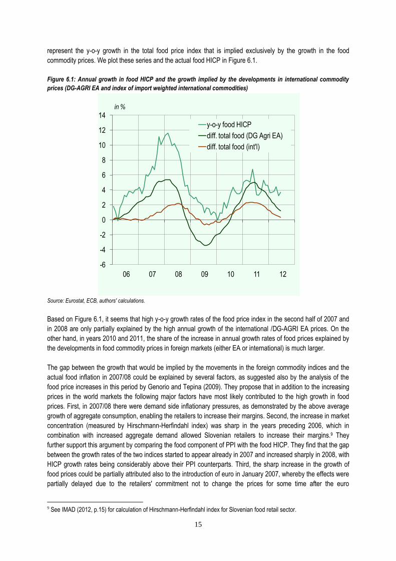
Figure 6.1: Annual growth in food HICP and the growth implied by the developments in international commodity
prices (DG-AGRI EA and index of import weighted international commodities)
Source: Eurostat, ECB, authors' calculations.
Based on Figure 6.1, it seems that high y-o-y growth rates of the food price index in the second half of 2007 and
in 2008 are only partially explained by the high annual growth of the international /DG-AGRI EA prices. On the
other hand, in years 2010 and 2011, the share of the increase in annual growth rates of food prices explained by
the developments in food commodity prices in foreign markets (either EA or international) is much larger.
The gap between the growth that would be implied by the movements in the foreign commodity indices and the
actual food inflation in 2007/08 could be explained by several factors, as suggested also by the analysis of the
food price increases in this period by Genorio and Tepina (2009). They propose that in addition to the increasing
prices in the world markets the following major factors have most likely contributed to the high growth in food
prices. First, in 2007/08 there were demand side inflationary pressures, as demonstrated by the above average
growth of aggregate consumption, enabling the retailers to increase their margins. Second, the increase in market
concentration (measured by Hirschmann-Herfindahl index) was sharp in the years preceding 2006, which in
combination with increased aggregate demand allowed Slovenian retailers to increase their margins.9 They
further support this argument by comparing the food component of PPI with the food HICP. They find that the gap
between the growth rates of the two indices started to appear already in 2007 and increased sharply in 2008, with
HICP growth rates being considerably above their PPI counterparts. Third, the sharp increase in the growth of
food prices could be partially attributed also to the introduction of euro in January 2007, whereby the effects were
partially delayed due to the retailers' commitment not to change the prices for some time after the euro
9 See IMAD (2012, p.15) for calculation of Hirschmann-Herfindahl index for Slovenian food retail sector.
-6
-4
-2
0
2
4
6
8
10
12
14
06 07 08 09 10 11 12
y-o-y food HICP
diff. total food (DG Agri EA)
diff. total food (int'l)
in %
16
introduction. Finally, according to Genorio and Tepina (2009), increased labour costs due to economic upturn and
increased costs of transport and fertilizers may have contributed to the higher growth in food prices in this period.
In addition, the gap between total HICP growth and the growth implied by international food prices is partially
explained also by the dynamics in tobacco prices that are subject to excise duty increases (see Section 2). This
holds for the entire period under inspection.
Another interesting observation is that the annual growth of food prices stemming from the DG-AGRI EA
commodity prices is much larger than the growth stemming from the developments in the international import
weighted food commodity index. This is in line with our results in Section 5, where we find that the EA DG-AGRI
prices are passed through to Slovenian food HICP to a larger extent.
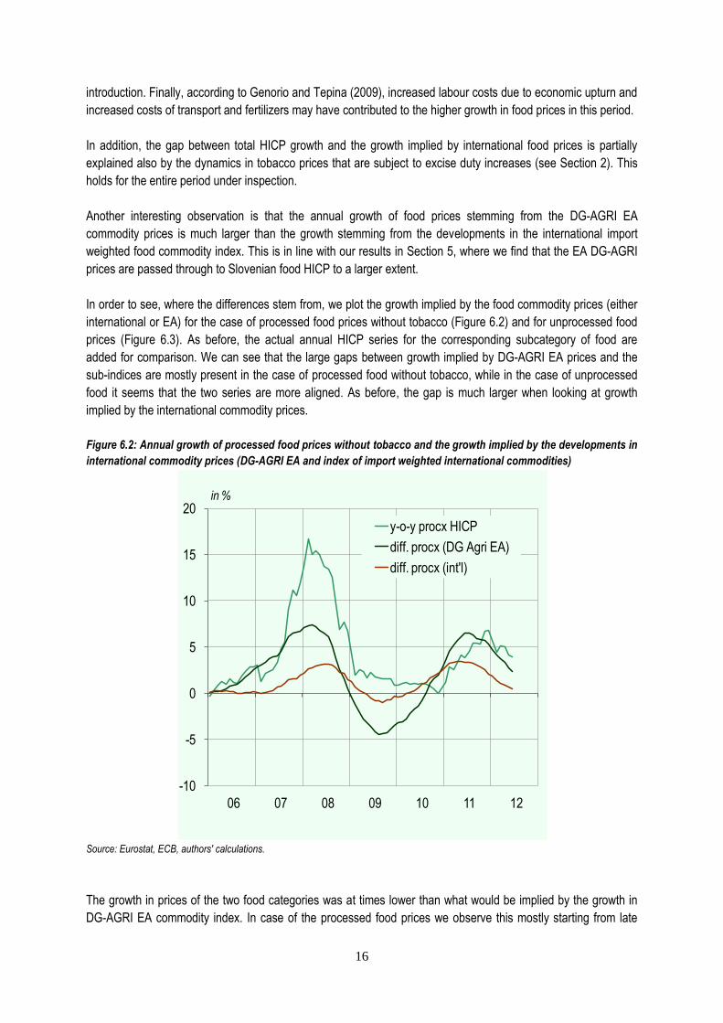
In order to see, where the differences stem from, we plot the growth implied by the food commodity prices (either
international or EA) for the case of processed food prices without tobacco (Figure 6.2) and for unprocessed food
prices (Figure 6.3). As before, the actual annual HICP series for the corresponding subcategory of food are
added for comparison. We can see that the large gaps between growth implied by DG-AGRI EA prices and the
sub-indices are mostly present in the case of processed food without tobacco, while in the case of unprocessed
food it seems that the two series are more aligned. As before, the gap is much larger when looking at growth
implied by the international commodity prices.
Figure 6.2: Annual growth of processed food prices without tobacco and the growth implied by the developments in
international commodity prices (DG-AGRI EA and index of import weighted international commodities)
Source: Eurostat, ECB, authors' calculations.
The growth in prices of the two food categories was at times lower than what would be implied by the growth in
DG-AGRI EA commodity index. In case of the processed food prices we observe this mostly starting from late
-10
-5
0
5
10
15
20
06 07 08 09 10 11 12
y-o-y procx HICP
diff. procx (DG Agri EA)
diff. procx (int'l)
in %
17
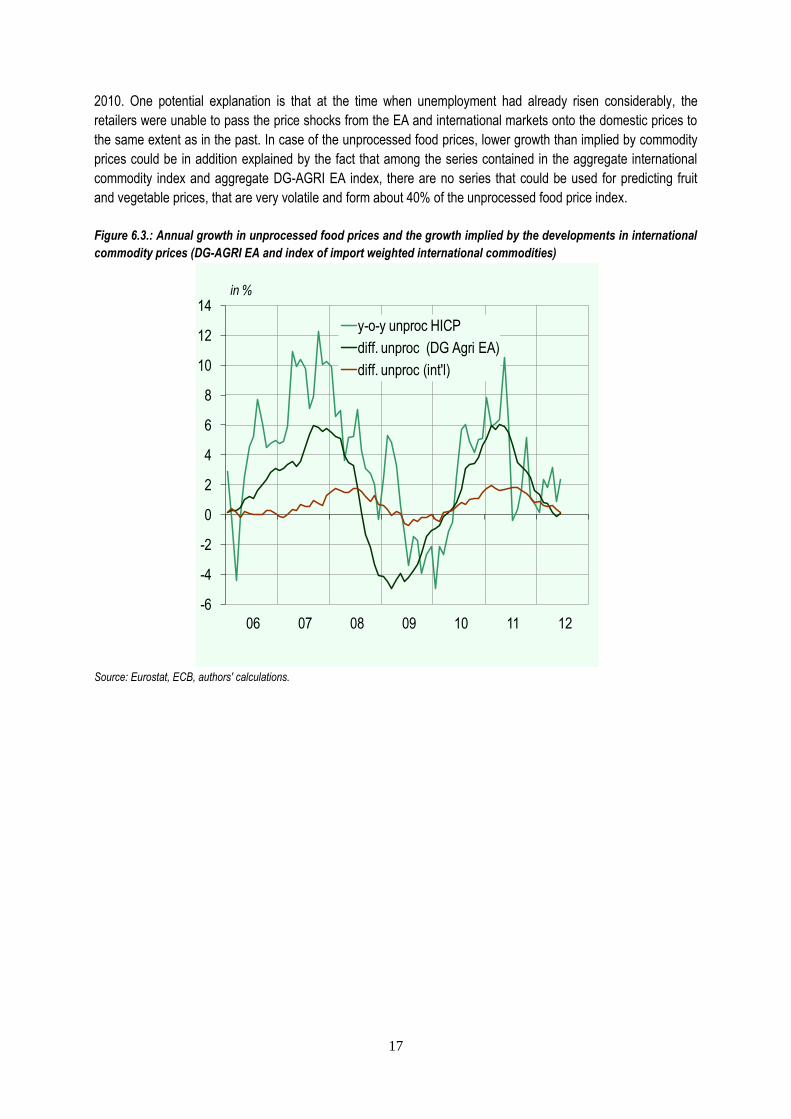
2010. One potential explanation is that at the time when unemployment had already risen considerably, the
retailers were unable to pass the price shocks from the EA and international markets onto the domestic prices to
the same extent as in the past. In case of the unprocessed food prices, lower growth than implied by commodity
prices could be in addition explained by the fact that among the series contained in the aggregate international
commodity index and aggregate DG-AGRI EA index, there are no series that could be used for predicting fruit
and vegetable prices, that are very volatile and form about 40% of the unprocessed food price index.
Figure 6.3.: Annual growth in unprocessed food prices and the growth implied by the developments in international
commodity prices (DG-AGRI EA and index of import weighted international commodities)
Source: Eurostat, ECB, authors' calculations.
-6
-4
-2
0
2
4
6
8
10
12
14
06 07 08 09 10 11 12
y-o-y unproc HICP
diff. unproc (DG Agri EA)
diff. unproc (int'l)
in %
18
7. Conclusion
In this policy note we aimed at assessing the extent of the pass-through of food commodity prices to the main
food HICP components, using a simple bivariate VAR where commodity prices are added as an exogenous
variable. In addition to the international food commodity prices, we used the newly available database of
commodity (farm-gate) food prices at the EA and national level constructed by the European Commission's DG-
AGRI and amended by the ECB.
The estimated pass-through is largest for EA level DG-AGRI prices, followed by Slovenian DG-AGRI prices.
International food commodity prices have a very small rate of transmission to domestic inflation. Independently of
the commodity index used, the effect of the price shock on annual inflation dies out in the third year after the
shock.
Looking at the sub-categories of food, we find that a shock to EA DG-AGRI prices passes through with about the
same magnitude to both, unprocessed and processed food (excluding tobacco) prices. A pass-through of a
similar magnitude is estimated for processed food prices in case of a shock to the Slovenian DG-AGRI prices. On
the contrary, unprocessed food reacts much less to shocks in Slovenian DG-AGRI prices, compared to shocks at
the EA level. International food commodity prices transfer to the domestic food prices in a much smaller extent
than EA DG-AGRI prices and the transmission is weaker in the case of unprocessed food prices compared to the
processed food prices.
To conclude, the model used for estimating the size of pass-through of shocks to different commodity indices
could be fruitfully used also for forecasting purposes, in particular for processed food without tobacco. We take
the first step towards using this model for forecasting by checking how well it fits the data using different
specifications in terms of lag length and type of commodity index used. We find that the model fits the data best
when using EA commodity prices and EA level PPI. One caveat related to using DG-AGRI prices for forecasting
purposes is that we need to form assumptions about future developments of these indices while not having any
guideline from the forward contracts that are used when forming assumptions about the international food
commodity index. In addition, further assessment of the forecasting performance would be needed before
integrating the model into regular projection exercise.
19
8. Literature
ECB (2011), "Recent Developments in Food Commodity Prices", Monthly Bulletin, No. 1, 2009, p. 13.
http://www.ecb.int/pub/pdf/mobu/mb201101en.pdf
EC - European Commission's Directorate General for Agriculture (EU DG-AGRI). (2012). [online] Available:
http://ec.europa.eu/agriculture/markets/prices/monthly_en.pdf
FAO – The Food and Agricultural Organisation. (2012). "FAO Food Price Index up 6 percent." [online] Available:
http://www.fao.org/news/story/en/item/154266/icode/
Ferrucci, G., Jiménez-Rodríguez, R. and Onorante, L. (2010), "Food Price Pass-Through in the Euro Area - The
Role of Asymmetries and Non-Linearities", ECB Working Paper, No. 1168.
Genorio, H. and Tepina, M. (2009), "Analiza in možni vzroki za porast cen hrane v Sloveniji v letu 2007", Prikazi
in Analize 1/2009, Banka Slovenije.
Koehler, A. B. and Murphree, E. S. (1988), "A Comparison of the Akaike and Schwarz Criteria for Selecting Model
Order", Journal of the Royal Statistical Society, Series C (Applied Statistics), Vol. 37, No. 2, pp. 187-195.
IMAD (2012), "Koncentracija v nespecializiranih pretežno živilskih prodajalnah na drobno", Ekonomsko ogledalo, No. 5 , Year XVIII, 2012, p. 15. http://www.umar.gov.si/fileadmin/user_upload/publikacije/eo/2012/EO0512_splet.pdf
20
A. Annex 1
Table A.1 AIC and SIC criteria - EA PPI, exchange rate included, model with wages
AIC - best
lag (p) AIC - value
SIC - best
lag (p) SIC - value
AIC - best
lag (p) AIC - value
SIC - best
lag (p) SIC - value
DG Agri EA 1 2 -14.31 2 -13.43 4 -16.34 2 -15.45
DG Agri EA 2 2 -14.33 1 -13.41 4 -16.37 1 -15.45
DG Agri EA 3 2 -14.31 1 -13.35 3 -16.37 1 -15.40
DG Agri EA 4 2 -14.29 1 -13.32 3 -16.35 1 -15.38
DG Agri EA 5 2 -14.28 1 -13.28 11 -16.33 1 -15.33
DG Agri EA 6 2 -14.25 1 -13.21 11 -16.30 1 -15.26
DG Agri EA 7 2 -14.23 1 -13.14 3 -16.29 1 -15.19
DG Agri EA 8 2 -14.31 1 -13.19 3 -16.34 1 -15.20
DG Agri EA 9 2 -14.28 1 -13.11 11 -16.32 1 -15.14
DG Agri EA 10 2 -14.26 1 -13.06 11 -16.29 1 -15.08
DG Agri EA 11 2 -14.24 1 -13.00 11 -16.31 1 -15.03
DG Agri EA 12 2 -14.22 1 -12.93 11 -16.33 1 -14.96
DG Agri Si 1 2 -14.14 1 -13.30 11 -16.30 1 -15.35
DG Agri Si 2 2 -14.13 1 -13.25 11 -16.28 1 -15.31
DG Agri Si 3 2 -14.10 1 -13.19 11 -16.27 1 -15.24
DG Agri Si 4 2 -14.12 1 -13.15 11 -16.25 1 -15.17
DG Agri Si 5 2 -14.10 1 -13.09 11 -16.22 1 -15.10
DG Agri Si 6 2 -14.09 1 -13.03 11 -16.20 1 -15.04
DG Agri Si 7 2 -14.07 1 -12.96 11 -16.17 1 -14.97
DG Agri Si 8 2 -14.08 1 -12.94 4 -16.17 1 -14.95
DG Agri Si 9 2 -14.05 1 -12.87 4 -16.14 1 -14.89
DG Agri Si 10 2 -14.05 1 -12.83 11 -16.13 1 -14.82
DG Agri Si 11 2 -14.04 1 -12.77 11 -16.15 1 -14.78
DG Agri Si 12 2 -14.01 1 -12.70 11 -16.13 1 -14.71
International 1 2 -14.13 1 -13.25 3 -16.20 2 -15.31
International 2 2 -14.12 2 -13.20 3 -16.19 2 -15.25
International 3 2 -14.14 1 -13.20 3 -16.18 1 -15.24
International 4 2 -14.14 1 -13.15 3 -16.17 1 -15.18
International 5 2 -14.13 1 -13.09 3 -16.14 1 -15.11
International 6 2 -14.10 1 -13.02 3 -16.17 1 -15.07
International 7 2 -14.08 1 -12.95 3 -16.14 1 -15.01
International 8 2 -14.05 1 -12.88 3 -16.11 1 -14.94
International 9 2 -14.02 1 -12.81 3 -16.09 1 -14.87
International 10 2 -13.99 1 -12.74 3 -16.07 1 -14.82
International 11 2 -13.97 1 -12.68 11 -16.06 1 -14.76
International 12 2 -13.95 1 -12.61 11 -16.05 1 -14.70
commodity index and
lags (m) included
Unprocessed food Processed food without tobacco
21
Table A.2 AIC and SIC criteria - SI PPI, exchange rate included, model with wages
AIC - best
lag (p) AIC - value
SIC - best
lag (p) SIC - value
AIC - best
lag (p) AIC - value
SIC - best
lag (p) SIC - value
DG Agri EA 1 2 -12.84 1 -12.04 5 -15.18 1 -14.31
DG Agri EA 2 4 -12.86 0 -12.02 4 -15.20 1 -14.28
DG Agri EA 3 4 -12.85 0 -12.00 4 -15.22 1 -14.24
DG Agri EA 4 1 -12.85 0 -12.01 4 -15.25 1 -14.25
DG Agri EA 5 0 -12.85 0 -11.97 6 -15.22 1 -14.19
DG Agri EA 6 0 -12.82 0 -11.90 6 -15.21 1 -14.12
DG Agri EA 7 0 -12.79 0 -11.82 6 -15.20 1 -14.05
DG Agri EA 8 0 -12.81 0 -11.80 6 -15.17 1 -13.99
DG Agri EA 9 0 -12.80 0 -11.74 6 -15.15 1 -13.93
DG Agri EA 10 0 -12.77 0 -11.67 6 -15.13 1 -13.86
DG Agri EA 11 0 -12.75 0 -11.61 12 -15.12 1 -13.80
DG Agri EA 12 0 -12.73 0 -11.55 6 -15.10 1 -13.75
DG Agri Si 1 1 -12.80 1 -12.01 10 -15.15 1 -14.31
DG Agri Si 2 1 -12.84 0 -12.05 10 -15.18 1 -14.32
DG Agri Si 3 1 -12.82 0 -12.00 10 -15.16 1 -14.25
DG Agri Si 4 1 -12.81 0 -11.94 11 -15.13 1 -14.18
DG Agri Si 5 1 -12.80 0 -11.89 10 -15.11 1 -14.11
DG Agri Si 6 1 -12.77 0 -11.82 10 -15.08 1 -14.04
DG Agri Si 7 1 -12.75 0 -11.75 10 -15.06 1 -13.98
DG Agri Si 8 1 -12.74 0 -11.69 10 -15.04 1 -13.91
DG Agri Si 9 1 -12.71 0 -11.63 10 -15.02 1 -13.85
DG Agri Si 10 1 -12.71 0 -11.59 10 -15.00 1 -13.78
DG Agri Si 11 1 -12.70 0 -11.53 11 -15.06 1 -13.74
DG Agri Si 12 1 -12.68 0 -11.46 11 -15.03 1 -13.67
International 1 1 -12.75 1 -11.96 3 -15.09 1 -14.27
International 2 1 -12.73 1 -11.89 3 -15.06 1 -14.20
International 3 1 -12.73 1 -11.85 10 -15.06 1 -14.16
International 4 1 -12.74 0 -11.83 3 -15.04 1 -14.11
International 5 1 -12.74 0 -11.80 3 -15.03 1 -14.06
International 6 1 -12.73 0 -11.74 3 -15.05 1 -14.01
International 7 1 -12.70 0 -11.68 3 -15.02 1 -13.95
International 8 1 -12.68 0 -11.61 3 -15.01 1 -13.90
International 9 1 -12.66 0 -11.55 3 -14.99 1 -13.83
International 10 1 -12.64 0 -11.47 5 -14.98 1 -13.79
International 11 1 -12.62 0 -11.41 11 -14.98 1 -13.74
International 12 1 -12.59 0 -11.35 11 -14.97 1 -13.67
Unprocessed food Processed food without tobacco
commodity index and
lags (m) included
22
Table A.3 AIC and SIC criteria for VAR, exchange rate included, model with wages
commodity
index
AIC - best
lag (p) AIC - value
SIC - best
lag (p) SIC - value
AIC - best
lag (p) AIC - value
SIC - best
lag (p) SIC - value
DG Agri EA 2 -19.75 1 -18.50 3 -21.81 1 -20.54
DG Agri SI 2 -19.40 1 -18.28 2 -21.45 1 -20.33
International 2 -17.77 1 -16.61 3 -19.83 1 -18.67
DG Agri EA 4 -18.34 1 -17.17 4 -20.72 1 -19.45
DG Agri SI 2 -18.05 1 -16.91 3 -20.36 1 -19.21
International 1 -16.43 0 -15.38 3 -18.75 1 -17.62
Unprocessed food Processed food without tobacco
1) VAR with PPI EA
2) VAR with PPI SI