food prices and household welfare: a pseudo panel · pdf filefood prices and household...
TRANSCRIPT

Food prices and household welfare:
A pseudo panel approach∗
Zacharias Ziegelhofer†
This draft: February 18, 2014
Abstract
The last years have seen an extra-ordinary surge in food prices and volatility. The aca-demic literature on its consequences currently focuses on the effect of high food prices inspecific regional and time contexts. This paper contributes to this literature in two ways:First, the analysis attempts to decompose the effect of global food prices on household wel-fare – i.e. is the effect driven by the trend, fluctuation around a trend, volatility or episodesof sustained price increases/decreases? Second, the paper extends the geographical andtime perspective on this issue and attempts to provide a worldwide picture of the impactof the recent surge in food prices. By taking a pseudo panel approach to this topic, thispaper can make use of a large amount of household information which is available fromrepeated cross sections of the Demographic and Health Surveys (DHS). The data subjectto this analysis contain information on about 500,000 individuals from 38 countries over aperiod of 20 years. Instead of following individuals over time as in a standard panel set-up,cohorts are followed over time. To remedy bias from measurement error in the context ofthe pseudo panel, the Verbeek-Nijman (1992) estimator, a variant of Deaton (1985)’s errors-in-variables model, is applied. The empirical analysis shows that adverse effects of foodprices on household welfare are transmitted through both short term-fluctuation in prices(volatility, period-to-period changes) as well as permanent price shocks (trend, episodes ofsustained price increases). There is mixed evidence on the impact of short-term fluctuationsaround a trend and periods of sustained drops in prices.
JEL Classification: C21, C23, D12, E31, I12, F61Keywords: food price, household welfare, child health, measurement error, pseudo panel,synthetic panel, Demographic and Health Surveys.
∗I thank Jean-Louis Arcand for his supervision and suggestions. I also thank Ugo Panizza, Cedric Tille, ThomasHelbling, Yi Huang, Lore Vandewalle, Rahul Mukherjee, Nicolas Berman, Matthias Rieger, Matthieu Stiegler,Katia Covarrubias, Julia Seiermann, Sven Kristen, Tehani Pestalozzi, Abbad El-Rayyes and the participants ofDevelopment Therapy Seminar in Geneva (December 2012 and October 2013) for their useful suggestions. Theusual disclaimer applies.†The author is a PhD Candidate in International Economics at the Graduate Institute of International and
Development Studies. Email: [email protected]
i

1 Introduction
The last decade has seen a stark increase in world food prices and food price volatility. From
the year 2000 until today, food price levels and volatility have more than doubled (see Figures
3 and 4).1 In this essay, I examine the consequences of this surge in food prices and volatility
on household welfare in developing countries. Previous research on this topic has concentrated
on the effect of high food prices (Von Braun and Tadesse, 2012) and has confined its analysis to
specific regional and time contexts. This essay contributes to the literature in two ways. First, by
decomposing the effect of food price variation in permanent shocks (trend), volatility, short- to
medium-term changes and sustained episodes of hikes and drops in prices. Second, by extending
the regional and time perspective of analysis through the application of a pseudo panel approach,
an idea first introduced by Deaton (1985).
The empirical analysis combines macroeconomic information on global food prices from the
International Monetary Fund (IMF) and the World Bank (WB) with household-level microe-
conomic data from the Demograhic and Health Surveys (DHS). This results in a pseudo panel
containing information on 38 countries during the period from 1991 to 2011. In the pseudo
panel approach, cohorts defined on the basis of a time-invariant characteristic are followed over
time. The resulting pseudo panel of cohort means may, therefore, suffer from measurement error.
To address this issue, I apply an errors-in-variables (EIV) model based on Deaton (1985) and
Verbeek and Nijman (1992). The choice of the appropriate estimator and cohort definition is
guided by Monte Carlo Simulations (MCS) which suggest that the Verbeek and Nijman (1992)
estimator is the best choice for the prevailing data situation.
Based on this methodology, I find that the variation in global food prices has a negative
impact on household welfare in developing countries. The impact is transmitted through the
long-term price trend, short-term changes in prices as well as volatility. I find mixed results on
the impact of short-term fluctuations around a trend and episodes of sustained drops in food
prices. To illustrate the magnitude of the above effects, I set the parameter estimates in relation
1In the media and public, the question of what role financial speculation has played in the surge of food priceshas been heatedly debated (Source: ”http://www.bloomberg.com/news/print/2011-01-24/speculation-swings-may-threaten-food-security-ministers-say.html”, site visited: July 26, 2013); public outrage has led some financialactors to cease or limit their engagement in commodity markets. In March 2012, bad press has led Deutsche Bankto suspend the creation of stock market traded financial products based on staple food commodities. In the mean-time, while some banks have withdrawn from financial speculation in food commodity markets. Some French,German and UK banks have withdrawn entirely from food commodity speculation. Among them are Volksbankenof Austria, Credit Agricole of France, Commerzbank, Landesbank Berlin, Landesbank Baden-Wurthemberg, DekaBank of Germany. Barclay Bank of the UK has announced on Feb 14, 2013, to stop speculation in food commodi-ties (Source: http://www.oxfam.org/en/pressroom/pressrelease/2013-02-18/key-eurozone-banks-step-back-food-speculation, site visited: November 1, 2013). Others, such as Deutsche Bank, have recommenced or continuedtheir activities, stating that there is no clear evidence that such products drive food prices or its volatility (Source:”https://www.deutsche-bank.de/cr/de/fokus/agrarrohstoffe.htm”, site visited: July 26, 2013).
1

to the effect size of education on child health and estimate the impact of the above food price
indicators on the rate of child malnutrition.
2 Literature review
Theoretical expectations of the effect of global food prices on domestic households are, a priori,
indeterminate and depend on macroeconomic factors as well as household characteristics.2 To
start, global commodity prices do not affect domestic producers and consumers directly and there
is no consensus as to which extent global prices pass through to domestic markets. Analyzing
FAO data from 1961-85, Mundlak and Larson (1992) have found that “most of the variation in
world prices are transmitted and that they constitute the dominant component in the variation
of domestic prices”. Hazell et al. (1990) argue that price variability has been fully transmitted to
developing countries but real exchange rate movements, domestic marketing arrangements and
government interventions have played a buffering role such that variability has not been fully
transmitted to producers’ selling prices. Morisset (1998) suggests that while upward movements
in prices are transmitted to domestic prices, downward movements are not or only imperfectly
transmitted to domestic consumer prices. Baffes and Gardner (2003) are more skeptical of
price transmission and find that market integration is high only for some countries and for
the remaining countries only few country-commodity pairs show pass-through of world price
changes. Dawe (2008) finds partial transmission of world prices to the seven Asian countries in
his sample. To sum up, even though the extent of transmission is subject to academic debate,
there is no doubt that world prices are, at least partly, transmitted to domestic markets whereby
the magnitude of pass-through may vary by country and commodity.
Given partial pass-through, global food prices may affect domestic households’ actions and
welfare. The micro-economic literature on the consequences of food price changes on household
welfare currently evolves in two directions: A literature which attempts to simulate the first-
order effects of increases in food prices and an empirical literature which examines the observed
2The price formation of commodity prices has been subject to academic scholarship for a long time. Historically,a large body of literature has evolved about the exploitation of a limited resource, the implied price paths of theresource (Hotelling, 1931) and sustainable pathways of growth in the face of limited resources. Krautkraemer(1998) undertakes an encompassing survey of this literature. Academic discourse has also evolved around the roleof competitive storage in price formation (Deaton and Laroque, 1996). More recently, there is a vivid debate onthe existence of super cycles (Erten and Ocampo, 2013) and the role of financial speculation (e.g. CBC (2008);Robles et al. (2009); Sanders and Irwin (2010)) in price formation. Headey and Fan (2008) assess the state of theliterature on the recent drivers of food prices. Among the discussed explanations, they find that commodity-widedrivers, in particular oil prices, the depreciation of the USD and biofuels have contributed to the rise in foodprices. The authors are rather skeptical of the following potential explanations for the recent hike in food priceswhich are also discussed in the literature: declining stocks, low interest rates and financial speculation. Apartfrom these general drivers of commodity prices, the authors find that also commodity-specific factors have playedan important role (in particular export restrictions for rice and to a lesser extent weather shocks for wheat).
2

consequences of the recent hike in food prices in specific regional and time contexts. In the
following, I will discuss the findings of these literatures in turn.
In his seminal paper, Deaton (1989) models how food prices affect households depending on
their position as a net producer or net consumer of agricultural goods. In his model, household
utility depends on wages, rental income, profits from farming or other business and prices. Deaton
(1989), then, derives an intuitive measure for the welfare change due to the price change, which
he defines as the amount of monetary compensation that a household would require to maintain
its previous level of welfare:
dB
x=(ωi −
piyix
)dln(pi) (1)
dBx is the amount of compensation expressed as a fraction of household expenditure x, ωi
signifies the expenditure share for good i, piyix is the value of production of good i as a share of
household’s total expenditure. Hence, ωi − piyix is the net consumption ratio which determines
whether households benefit or are hurt from price increases in the short run. This approach
abstracts from medium- to long-term adjustments in consumption and production decisions by
the household in response to the changed price.
Framing the issue in terms of net producers versus net consumers as outlined in Deaton’s
(1989) model has become the predominant approach to the analysis of microeconomic conse-
quences of food price shocks. Many authors have used this framework to simulate first order
effects of an increase in food prices (e.g. Deaton (1989); Barrett and Dorosh (1996); Zezza et al.
(2008); Ivanic and Martin (2008); Wodon et al. (2008); Aksoy and Isik-Dikmelik (2008)). Others
have taken a related approach and simulated the impacts of food price shocks based on previ-
ously estimated demand systems (e.g. Anrıquez et al. (2013); Iannotti and Robles (2011)) or
Computable General Equilibrium (CGE) models (e.g. Arndt et al. (2008)).
Overall, the literature suggests that adverse effects of increased food prices outweigh positive
effects for the poor in most developing countries, at least in the short run (Zezza et al. (2008);
Ivanic and Martin (2008); Iannotti and Robles (2011)). The poor spend a high share of their total
expenditure on food (Deaton, 1989; Cranfield et al., 2007) and are predominantly net consumers,
not only in urban but also often in rural areas (Arndt et al., 2008; Ivanic and Martin, 2008; Aksoy
and Isik-Dikmelik, 2008), which makes them vulnerable to food price shocks. On the other side
of the equation, there are also winners to increased prices. Zezza et al. (2008) find that those
3

with access to land and productive inputs to agriculture can gain – even if they are part of the
poorer households.3
There are further exceptions to the stylized fact that price increases are hurting lower income
households: Based on his model and data on household food expenditures and production in
Thailand, Deaton (1989) predicts that higher prices for rice are overall beneficial to rural house-
holds at all wealth strata in Thailand. Strikingly, the benefits of higher rice prices do not tilt
the income distribution towards the rich; it is the middle income farmers who benefit most, as
net sales make up for an important portion of their income while relatively few rich are engaging
in rice farming (Deaton, 1989). Aksoy and Isik-Dikmelik (2008)4 find that even though most of
the poor are net buyers of food, almost half of them are only marginal net buyers and would
hence not be hit very hard by increases in food prices. Because most of the rich do not engage in
agriculture, an increase in food prices shifts income from higher incomes to lower incomes. This
finding changes when the authors confine their analysis to the poor only: Among the poor, net
sellers are richer than net buyers in five countries and net buyers only in one country subject to
their analysis.
Furthermore, the impact of food price hikes can be heterogeneous according to the specific
commodity and country. For instance, even though Ivanic and Martin (2008) predict that for
most countries of their sample5 the welfare losses of the relatively poor outweigh the gains
resulting in increased overall poverty (both in terms of poverty headcount and poverty gap), beef
is an exception to this pattern. Increases in the price of beef are predicted to reduce poverty in
Cambodia and Peru.
Ravallion (1990) develops a framework which also takes into account adjustments in agricul-
tural wages. He derives conditions under which households in rural poor areas, which are net
suppliers of labor and net consumers of agricultural goods, can benefit from increases in food
prices: If the price elasticity of the wage rate exceeds the net food expenditure to income ratio,
the rural poor can gain from increases in food prices. Ravallion (1990) applies this theoretical
framework to the case of Bangladesh and finds that, in the short run, the rural poor are nega-
tively affected by price increases (while the rural rich gain) but the welfare effect is rather neutral
in the long run after adjustments in wage rates. The welfare effect varies among the poor with
3The analysis is based on information from the RIGA database on eleven countries (Africa: Ghana, Malawi;South and East Asia: Bangladesh, Nepal, Pakistan, Vietnam; Eastern Europe and Central Asia: Albania, Tajik-istan; Latin America: Guatemala, Nicaragua, Panama)
4The authors examine the characteristics of net food buyers and sellers in the eight countries Bangladesh,Cambodia, Vietnam, Bolivia, Nicaragua, Peru, Ethiopia, Madagascar and Zambia.
5Bolivia, Cambodia, Madagascar, Malawi, Nicaragua, Pakistan, Peru, Vietnam, Zambia
4

likely positive effects for the very poor; however, in general, positive effects can only be expected
to outweigh the negative effects after three to four years.
Dessus et al. (2008) have attempted to quantify the welfare effects of the recent increases
in food prices on urban households and find that the compensation costs of the 2005-7 increase
in food prices represent less than 0.2 per cent of GDP for most countries. However, for some
countries the cost can exceed 3 per cent. The welfare losses are mainly due to the negative real
income effect on households which were already poor before the price hike. “New” households
falling into poverty only represent a small share of the cost.6,7
The literature discussed so far relies on Deaton’s model, estimated demand systems and to a
lesser extent CGE models. This literature has made an important contribution in predicting first
order effects, developing conditions under which the rural poor can gain (loose) and in identifying
vulnerable households which can be expected to experience negative consequences of increases in
food prices – a question with great relevance and importance, especially, for the design of policies
which aim to mitigate the consequences of the recent hikes in food prices. However, this literature
still leaves room for future research. First, the empirical analyzes usually exploit either descriptive
information on expenditure shares and production or use between individual heterogeneity to
determine the response of households to price increases. It is not clear how households react when
they are hit by more extreme shocks (crisis times) and whether the association of consumption
and food prices is the same between households and within households over time. Second, all
of the simulation approaches rest on complex methodologies which themselves rely on a number
of assumptions (e.g. in the construction of a poverty line, a minimum caloric intake). Results
may be sensitive to the chosen assumptions, even if reasonable and necessary for simplification,
and to the distribution of individuals around the constructed thresholds. Third, the focus on
simulations has led to relatively little attention to the “observed” consequences of changes in
food prices on household welfare in the academic literature8 and for this reason needs to be
complemented with empirical approaches.
6Dessus et al. (2008) estimate the monetary cost (based on the change in an Atkinson (1987)-style “povertydeficit”) to compensate for the costs of the 2005-7 increase in food prices based on the Global Income DistributionDynamics (GIDD) dataset which comprises 72 household surveys on low and middle income countries.
7Anrıquez et al. (2013) come to a similar conclusion in finding that many poor were already undernourishedbefore the hike in food prices. Anrıquez et al. (2013) simulate households’ food demand responses to a food priceshock based on estimated demand systems in 8 countries using the survey database RIGA. In doing so, the authorsuse nutritional attainment as a measure of welfare. In this approach, persons are considered undernourished whenthey fall below a minimum energy requirement. The authors find an increase in undernourishment as a consequenceof price increases; the effect is less pronounced for the poor because many of them are already below the minimumenergy requirement. The impact is mainly driven by the three factors: dietary patterns (reliance on the mainstaple foods), staple farm income and the concentration of households around the dietary threshold. The authorsfurther decompose the effect in mean and distributional effects and find that the distributional effect increasesundernourishment in most of the analyzed countries.
8In the policy world, there is a large amount of case studies and qualitative research available on theconsequences of food prices and qualitative and quantitative assessments of the effectiveness of interven-tions carried out by organizations working on Food Security such as the World Food Program (source:
5

There have been attempts to estimate the empirical effects of high food prices in particular
regional and time contexts. These empirical studies mainly focus on child health as a dependent
variable and their results are mixed: Some studies find a negative effect of high food prices on
child health and some cannot identify such an effect.
Block et al. (2004) estimate the impact of Indonesia’s drought and financial crisis in 1997/8
on child health measured by weight-for-age (WAZ).9 Interestingly, the WAZ of children remained
constant during the crisis despite the surge in food prices. The authors suggest that mothers
buffered the nutritional impact on their children resulting in observed increased maternal wasting.
In addition, the authors find that micronutrient status declined for both women and children
and observe higher incidence of maternal and child anemia.
Waters et al. (2004) analyze child health status (WAZ) in Indonesia from 1992-1999 based
on pooled cross sectional data. They find that the household characteristics of family income,
mother’s education and source of water are predictors of higher WAZ. In line with the analysis
of Block et al. (2004), the authors could not identify an effect of the 1997-99 crisis (which went
hand in hand with increases in food prices) on child health. However, during 1997 to 1998
adult malnutrition (measured by Body Mass Index, BMI) did slightly deteriorate which the
authors interpret as a possible consequence of parents trying to shield their children from health
consequences “at their own expense”.10
Sulaiman et al. (2009) compare child health status in Bangladesh in 2006 and 2008 – years
which have seen stark increases in rice (increase of over 94 per cent) and wheat prices (increase
of over 106 per cent). The authors run paired t-tests to investigate the change in childrens’
weight-for-height z-score (WHZ) and mothers’ BMI. For the rural sample for which panel data
is available, the authors also apply a multivariate regression model with household fixed effects.
For the urban sample, the analysis relies on cross sectional data. Sulaiman et al. (2009) find a
significant deterioration11 in child health (WHZ) for both rural and urban areas of the magnitude
of approximately -0.1 standard deviations (SD). In the same period, mothers’ BMI had improved
significantly in rural areas and had not changed significantly in urban areas. The effect of food
prices is estimated by a year-dummy for the year 2008. Hence, all variation in WHZ which is
collinear with this dummy is attributed to the price effect. In their quantitative and qualitative
analyzes, the authors find evidence that the composition of children’s (and households’) diets
http://www.wfp.org/content/revolution-food-aid-food-assistance-innovations-overcoming-hunger, site accessed:Nov 3, 2013).
9In their analysis, the authors create birth-cohorts based on fourteen repeated cross sections and decomposetrends into time, age and cohort effects.
10This effect has been described as “sacrifice effects” in other contexts, see Li and Wu (2011).11For urban households, the result is only significant at the 10 per cent level of significance.
6

changed and suggest this could be the primary mechanism through which the worsening of child
health status operated.
In his analysis of the patterns of food consumption and nutrition in Bangladesh, Ahmed
(1993) analyzes the consequences of a 20 per cent fall in rice prices from the lean season 1991
to 1992. Based on data collected by the International Food Policy Research Institute (IFPRI),
the author finds that households are highly responsive to this change and decreased their wheat
consumption to increase their rice, meat, milk and egg consumption as well as overall calorie
intake. At the same time, adult nutritional status improved and a decrease in undernourished
children was observed.
De Brauw (2011) analyzes the role of remittances in mitigating the adverse effect of food price
shocks in El Salvador based on survey data from 2008. During 2008, El Salvador experienced a
15 per cent increase in food prices which was associated with a deterioration in the child height-
for-age z-score (HAZ) by 0.2 SD on average. De Brauw (2011) found that, during the period of
the price hike, households that send out migrants and/or receive remittances from abroad tended
to have higher child HAZ.
In the context of Malawi, Wood et al. (2012) analyze whether agricultural households who
focus on cash crop production are more vulnerable to price shocks than those who engage in
traditional maize farming. In 2001, due to severe drought, Malawi experienced a sharp increase
in maize prices. Based on the 2004-5 nationally representative Malawi Integrated Household
Survey, the authors investigate whether the in utero exposure to this food price shock has led to
deteriorated health status (HAZ) in children later on. Using an instrumental variables approach,
Wood et al. (2012) find that while during stable times there is no effect of cash crop production on
child health status, there is a negative association between child health and households engaging
in cash crop farming during the 2001 increase in maize prices. This result indicates that children
of cash crop producers are more vulnerable to food price shocks in staple foods such as maize.
Finally, if child health is understood as the outcome of a child health production function,
several inputs have to be considered in addition to the food price shocks. A related literature has
identified determinants of malnutrition, mainly focusing on household-level determinants (e.g.
Hadley et al. (2012); Nakabo-Ssewanyana (2003); Saha et al. (2009)).12,13 In their meta-analysis
of the academic literature on child nutritional status and mortality, Charmarbagwala et al. (2004)
12Nakabo-Ssewanyana (2003) find that in Uganda households with older women, larger household size, lowerfemale education and low income are more likely to have malnourished children.
13Hadley et al. (2012) found that maternal distress is associated with lower child health and some portion ofthe food insecurity effect is mediated through this variable.
7
identify the socio-economic factors which have been found to determine child health.14 Those
factors are of great relevance for this essay and for this reason, if they dispose of sufficient
within-cohort variation and are feasible to implement, are included as control variables.15 Char-
marbagwala et al. (2004) find that the overall evidence in the literature indicates a significant
negative effect of mother’s education, household wealth, access to water and sanitation on child
mortality and a positive effect on nutritional status. The authors also find a negative effect of ac-
cess to electricity on child mortality and a positive effect of an urban dummy, father’s education
and a female-headed household dummy on nutritional status.
A related literature has found that early health status has persistent effects in determining
later life outcomes such as health status and educational outcomes (e.g. Alderman et al. (2001,
2006); Porter (2010)). This literature links to Heckman and Cunha’s (2007) theoretical work on
the technology of skill formation which points to (dynamic) complementarities between different
dimensions of child development and emphasizes the importance of early child development for
later outcomes. Porter (2010) shows that in the context of Ethiopia, food aid had a positive
and lasting impact on later health status (ten years later).16 Successful examples like the one
analyzed by Porter (2010) demonstrate that the hands of policy makers are not tied when food
price shocks occur. For the design of policies and programs which succeed in delivering enhanced
food security and health, it is essential to better understand how households are affected by food
price shocks.
The empirical micro-economic literature has so far confined its analysis to specific regional and
time contexts. Furthermore, due to the mainly cross-sectional nature of analysis, the literature
was unable to decompose the price variation and to attribute the effects to specific components of
the variation in food prices – i.e. are the results driven by the trend, fluctuation around the trend
or volatility? This essay intends to contribute to the literature by providing insights into these
questions and by broadening the regional and time scope of analysis. Based on information on
approximately 500,000 children covering 38 countries in the period from 1991 to 2011, I provide
a world wide picture of how the variation in food prices has affected household welfare.
14The authors also evaluate the effect of biological and demographic factors and health services on child healthfrom which I abstract in this study.
15The household-level controls include an urban dummy, years of education of the mother and male partner, em-ployment in agriculture or self-employment in agriculture, improved water facilities, improved sanitation facilitiesand a wealth index. No control for female-headed households is included in the analysis.
16The author also finds that stunting in early years doubles the probability of stunting in early adolescence.
8

3 Research question and model
In their review, Von Braun and Tadesse (2012) find “that the current body of literature con-
centrates on high food prices” and stress the importance to differentiate between types of price
changes which reflect long-term (trend) and short- to medium-term price changes (volatility,
spikes). The aim of the following empirical analysis is to bridge this gap in the literature by
decomposing the variation in food prices in volatility (coefficient of variation), price spikes (price
change in per cent), trend, short-term fluctuation, and sustained periods of price increases and
decreases, which I will refer to as price hikes and price drops.17 The analysis, then, attempts to
identify the impact of these types of variation in food prices on household welfare. I choose to
proxy household welfare, with child health18 and operationalize child health as the weight-for-age
z-score (WAZ) which is sensitive to short-term changes in child health19. The change in WAZ is
a good proxy for household welfare effects for two reasons:
First, “when food price or income shocks occur, poor households adopt a series of food and
nonfood coping strategies to protect their basic needs; in this context, maintaining their energy
consumption level is one of their most fundamental concerns” (Ruel et al., 2010). Food coping
strategies may include reducing calorie intake, switching to cheaper and lower quality foods and
changing the intra-household allocation of resources. These strategies may have direct adverse
consequences for household members, in particular children (Ruel et al., 2010). Other non-
food coping strategies (e.g. wife seeking outside employment, child labor, reduced spending on
education and other non-food expenses) may only show negative consequences in the longer-
term. When investment in child human capital (health, education) is constrained, this is likely
to perpetuate inter-generational poverty transmission (Ruel et al., 2010).
The existence of food and nonfood coping strategies and different time-horizons in the real-
ization of impacts on household welfare has implications for the interpretation of the econometric
analysis in this essay: If effects on the nutritional and health status of children can be observed,
this signifies that the shock must translate into the households with considerable strength such
that the households are not able to absorb those shocks through neither insurances and capital
markets nor the mentioned coping strategies which do not rely on reducing or changing food
consumption. If, nevertheless, an effect is identified, we can assume that the price changes have
had strong effects on the household welfare – likely beyond child health. Therefore, child health
can be considered a conservative indicator for the consequences of food price shocks.
17For the definition of the concepts, see data and definitions.18In this analysis, the term “child health” refers to the health status of children until the age of five.19For more technical information on the calculation of the indicator, see the section data and definitions.
9

Second, child health is a meaningful development indicator as it also predicts some longer-term
consequences of food price shocks: Early child health is an important determinant of later health
status (Alderman et al., 2006), education (Alderman et al., 2001) and wealth (Currie, 2009); for
this reason, child anthropometrics also capture long-term consequences of price shocks.
In the below model, child health20, as a proxy for household welfare, is regressed on the food
price indicators (FPI, Figures 3 and 4) and a set of control variables which have been identified
by the literature as major determinants of child health status. The control variables include
access to improved water supply and sanitation infrastructure, years of education of the mother
and father, employment status (agricultural employment, agricultural self-employment, other),
a wealth index, logarithmic GDP per capita and a time trend tt. The time trend is included to
control for an overall trend in macroeconomic variables which may otherwise be captured by the
coefficients on the food price indicators (in particular the food price index and the trend). The
model is formalized in equation 2 whereby the index int refers to a given individual i, in country
n at time t, αi is individual-specific time-invariant heterogeneity and ε is an error term.
WAZint = β0 + β1FPIt + β2 improved water supplyint + β3 improved sanitationint
+ β4 maternal educationint + β5 paternal educationint
+ β6 agr. employmentint + β7 agr. self-employmentint
+ β8 urbanint + β9 wealthint + β10 GDPnt + β11tt + αi + ε (2)
In the following section, I describe the identification strategy of this essay which is based
on Deaton’s (1985) error-in-variables model for repeated cross sections. The approach allows
combining macroeconomic data on global food prices with microeconomic data at the household
level while controlling for individual effects αi.
20The anthropometric measure WAZ is calculated for children until the age of five. This reflects the dataavailability of the DHS surveys.
10

4 Identification strategy
To lay out the identification problem, it is informative to start off with a simple linear model
of pooled cross-sections. In doing so, I rely on Verbeek’s (2008) discussion. Equation 3 states
the model whereby yit denotes the health status of child i at time t, x′it is a K-dimensional
vector of explanatory variables, αi is an individual fixed effect and β is the coefficient vector
of interest. If the individual effects αi were uncorrelated with the explanatory variables, we
could estimate the model consistently by pooling the repeated cross sections and running an
OLS estimation on the pooled sample. Even though this assumption has the potential to greatly
simplify our lives (and is frequently made in empirical approaches), it does not seem realistic
in the context of our estimation problem: Some of the explanatory variables are household and
individual characteristics and it is therefore likely that they are correlated with the individual
effects. Let’s assume Exituit = 0 and Exitαi 6= 0.
yit = x′itβ + αi + uit, t = 1,...,R and i = 1,...,N (3)
When some of the explanatory variables are correlated with the individual effects, then at
least some of the K moment conditions E(yit − x′itβ)xit = 0 are invalid, resulting in biased
estimates for all coefficients β. In the context of a panel structure, this issue can be remedied
by the use of a within-individual estimator (fixed-effects estimator) controlling for all individual-
specific time-invariant heterogeneity. In the absence of genuine panel data, this option is not
available due to a lack of information on the individuals’ history. In his seminal paper, Deaton
(1985) suggested that, in situations where repeated cross sections are available, one can resort
to a cohort-based pseudo panel approach in which the idea is the following:
Based on the model in equation 3, C cohorts which consist of individuals with a common
time-invariant characteristic can be defined. The time-invariant characteristic should assign each
individual to a unique cohort. This assignment needs to remain the same across time such that
if an individual from an earlier cross section would be drawn into one of the samples of a later
cross section, it would end up in exactly the same cohort. In this essay, cohorts are defined based
on birthyear brackets and the country of residence.21 By transforming the pooled cross section
to a model of cohort means using this cohort definition, we obtain the pseudo panel (or synthetic
panel) model in equation 4.
21I abstract from migration between countries. This simplification is realistic for the largest part of the house-holds and is for this reason unlikely to influence the results.
11

yct = xctβ + αct + uct, c = 1,...,C and t=1,...,R (4)
Choosing a meaningful cohort definition is crucial to this approach because the parameters
can only be identified if the cohort definition generates sufficient variation over time (Verbeek,
2008). The pseudo panel now contains T = C×R observations with c referring to the individual
cohorts and t to the time period. As in its cross-sectional counterpart, the explanatory variables
xct from the synthetic panel are likely to be correlated to the individual cohort effects αct. Letting
αct be subsumed by the error term will lead to biased estimates as not all K moment conditions
E(yct − x′ctβ)xct = 0 can be expected to hold.
If we replace αct with αc (i.e. αct is replaced by cohort dummy variables), one can then
estimate the model in 4 by OLS or weighted least squares if cohort sizes vary greatly; this
estimator has been referred to as the efficient Wald estimator (Angrist, 1991; Devereux, 2007b).
In small samples, this estimator is biased due to cov(αct − αc, xct) 6= 0 (Devereux, 2007b, p.
840).
Until today, there is no consensus in the academic literature as to what cohort size is deemed
sufficiently large. While Verbeek and Nijman (1992) consider that “the effects of ignoring the
fact that only a synthetic panel is available will be small if the cohort sizes are sufficiently
large (100, 200 individuals)”, Devereux (2007b) shows that in practice considerable biases can
emerge when pseudo panel models are estimated based on cohorts which consist of a size of
100-200 individuals without correcting for sampling errors. Devereux (2007b, p. 839) finds that
for his particular application, the estimation of the income elasticity of female labor supply,
“thousands of observations per group are required before small-sample issues can be ignored in
estimation[...]”. Even with cohort sizes of 10,000 observations per cohort, biases of the order of
10 % still persist (Devereux, 2007b).
In applied research, we often encounter heterogeneous cohort sizes of which some are well
below 100 individuals per group. To remedy bias due to small cohort size, this essay resorts to
Deaton’s (1985) approach which corrects for measurement error. Again, the choice of whether or
not an EIV estimator is necessary essentially boils down to one’s decision on a set of asymptotic
assumptions.
Deaton (1985) assumes fixed cohort size nc while the number of cohorts C tends to infinity
(C →∞). These two assumptions seem realistic in our context where birthyear-country-cohorts
are formed and cohort size can be small, sometimes with nc < 100. When more rounds of
12

household surveys become available, this increases the number of cohorts in the dataset but
does not affect cohort size. Other authors (e.g. Moffitt (1993)) have assumed that the number
of individuals per cohort tends to infinity (nc → ∞) while C is constant. If the second set of
assumptions were applied, one could conveniently abstract from the measurement error problem.
In this essay, I assume that measurement error is substantial and understand the estimation
problem as an errors-in-variables problem. If equation 5 is the true cohort model, then the
cohort sample means yct and xct in equation 4 are error-ridden estimates of this true model. The
individuals which constitute a cohort in the microdata can be considered random draws from
the true population22. The expected value of the cohort means is the true population mean and
the measurement error variance declines with increasing cohort size according to the law of large
numbers.
y∗ct = x∗ctβ + α∗ct + uct, c = 1,...,C and t=1,...,R (5)
In following Deaton’s (1985) notation, equation 5 can be simplified to equation 6 with a
single index t, running from 1 to T. Now, x∗ct also contains the cohort dummies which are not
subject to measurement error and are treated as being measured with an error of zero mean and
variance. This can also extend to other variables such as country characteristics which do not
have the measurement error structure of equation 7. To warrant Deaton’s (1985) assumption
of the error ut to be normal, homoskedastic and independent over t, the observations need to
be weighted by the inverse of the square root of cohort size. The weighting23 can be obtained
by premultiplying all variables by a diagonal weighting matrix V −1/2 which is defined such that
P = P ′ = V −1/2V −1/2 = V .
y∗t = x∗tβ + ut, t=1,..., CR︸︷︷︸=T
(6)
22Obviously, this assumption only holds if the underlying sampling was representative of the true populationwhich we assume is the case in the Demographic and Health Surveys which are subject to this analysis.
23For more details, see Greene (2007) or other standard econometric texts.
13

Deaton (1985) assumes the following measurement structure which corresponds to the prop-
erties of classical measurement error:
ytxt
= N
y∗t ; σ00 σ′
x∗t ; σ Σ
(7)
Following Verbeek’s (2008) notation, the above measurement error structure can be re-written
as
yt − y∗txt − x∗t
= N
0; σ00 σ′
0; σ Σ
(8)
whereby the true populations values y∗t and x∗t can be interpreted as unknown but constant
terms. From this notation, it can be seen that the measurement error variances of yt − y∗t and
xt − x∗t reduce to the variance of the respective means:
σ00 = var(yt − y∗t ) = var(yt) + var(y∗t )︸ ︷︷ ︸=0
− 2 cov(yt,y∗t )︸ ︷︷ ︸
=0
= var(yt) (9)
In analogy to the above, Σ = cov(xt). Consequently, the covariance vector σ can be derived
as follows24:
cov(yt − y∗t ,xt − x∗t ) = cov(yt,xt) = cov(βxt + ut,xt)
= β × 1× var(xt) + 1× 0× var(ut)︸ ︷︷ ︸=0
+(β × 0 + 1× 1) cov(xt, ut)︸ ︷︷ ︸=0
= βvar(xt)
(10)
Since we assume the measurement error to be classical following a normal distribution with
zero mean, the moments are well understood. Following Fuller (1981), let us assume Wt =
W0t = (yt−y∗t ),W1t = (x1t−x∗1t), ...,Wkt = (xkt−x∗kt) are random variables whose realizations
constitute draws from a multivariate normal distribution with mean zero and covariance matrix
χ, where σij are the elements of χ. To clarify notation, syy = s11 = σ00, the elements of σ are
syxk = s1k and the elements of Σ are denoted sxjxk = sjk with j = 2, ..., k+1 and k = 2, ..., k+1.
24Using the following property of expectations in a joint distributions cov(ax + by, cx + dy) = acvar(x) +bdvar(y) + (ad+ bc)cov(x, y), we obtain the next equation (see Greene (2007, p. 1004)).
14

We know from the properties of moments of the normal distribution (see Fuller (1981)) that
the sample mean has the variance EWiWj = n−1c σij . This property can be used to estimate
the respective measurement error variances in pooling the cross-sectional datasets. After the
cohort means have been removed from the data, σ00, Σ and σ can be estimated by their sample
counterparts s00, Sjk and sj , as described in the below equations.
s00 = var(yt − y∗t ) =σ2y
nc(11)
The diagonal elements of Σ can be estimated
Sjj = var(xjt − x∗j ) =σ2xj
nc(12)
while the off-diagonal elements are estimated by
Sjk = cov(xjt − x∗j t, xkt − x∗k) =σxjxknc
(13)
and the elements of σ by
syxj = cov(yt − y∗t ,xt − x∗t ) =σyxnc
(14)
Based on Fuller (1975, 1981), Deaton (1985) derives the error-in-variables estimator in equa-
tion 15. This estimator yields identical results to the jackknife instrumental variables estimator
and is closely related to the k-class of instrumental variables estimators (Devereux, 2006).
β = (Mxx − S)−1(mxy − s) = (X ′X − TS)−1(X ′y − Ts) (15)
whereby Mxx and mxy are the respective sample moments and cross product matrices, S and s
are the sample counterparts of Σ and σ and Ω = Mxx − S.
Under the assumption of known error variances, Deaton (1985) derives the variance of the
estimator as follows25
TV (β) = Ω−1[T−1X ′Xe′e+ T−2X ′ee′X
]Ω−1 (16)
25This assumption does not greatly change the estimates as will be seen in the empirical part of this essay.
15

Under the assumption of estimated error variances, the variance of the estimator becomes
slightly more complicated (Deaton, 1985) but can be evaluated straightforwardly in practice.
TV (β) = Ω−1[Σxxω
2 + (σ − Σβ)(σ − Σβ)′]
Ω−1 + v−1Ω−1V (s− Sβ)Ω−1 (17)
whereby Σxx = E(Mxx), ω2 = 1T e′e and V (s−Sβ) = Σ(σ00− 2σ′β+β′Σβ) + (σ−Σβ)(σ−Σβ)′
and v = nc.
Verbeek and Nijman (1992) suggest a slightly altered estimator which provides better prop-
erties when only few repeated cross sections are available. The estimator is written down in
equation 18 whereby τ = (P −1)/P and P indicates the number of repeated cross sections which
are available for the cohorts.26
β = (Mxx − τS)−1(mxy − τs) (18)
Which approach fits the data best depends on the specific characteristics of the data. In
section 9.10, I explore the properties of various estimators using Monte Carlo Simulations (MCS)
based on a data generating process which mimics the data availability. The results from the
simulations clearly suggest that the Verbeek-Nijman (1992) estimator outperforms the other
estimators (OLS, Cohort Fixed Effects / Efficient Wald and Deaton (1985)) in this context.
26Similarly, Devereux (2007a) suggested an estimator that is approximately unbiased in the case of a smallnumber of cohorts.
16

5 Data and definitions
The data which underlie this analysis are assembled from three different sources: The Demo-
graphic and Health Surveys (DHS)27, the Commodity Price Indices by the International Mone-
tary Fund28 and the World Development Indicators from the World Bank29.
The DHS survey data are ideal as basis for pseudo panel analysis due to their richness in
demographic and health information, comprehensive regional coverage, repeated implementation
and high degree of standardization between countries and survey rounds. Currently, more than
300 DHS surveys from more than 90 countries are available upon request. The questionnaires
of the surveys follow six templates depending on the phase of survey implementation (DHS I to
DHS VI). To merge several DHS surveys to a pooled and coherent dataset has obvious challenges.
Some information is only available in certain survey phases (and for certain countries) and some
variables are coded with country-specific values. Nevertheless, compared to other sources of
survey data (e.g. World Bank Living Standards Measurement Study, LSMS), the DHS data is
characterized by a high degree of standardization which is crucial for the chosen pseudo panel
approach.
All available survey rounds (210 by early 2013) with several repeated cross-sections for a given
country and which contain the relevant information for the question of analysis were pooled into
one dataset. After the omission of missing values, the pooled child-recode dataset contains
information on 497,839 children and their households from 38 countries (see Table 1). This
information was then merged with the macroeconomic information on world food prices from
the IMF and the World Bank and GDP per capita from the World Bank.
Child health, used as a proxy for household welfare, is measured by an anthropometric indi-
cator, the weight-for-age z-score (WAZ)30. The WAZ of a child is defined as the distance between
the weight-for-age ratio of the given child compared to the median of a reference population31
(of the same age and sex) divided by the standard deviation (SD) of the reference population.
Pathological deficiencies indicated through WAZ are referred to as “underweight”. Usually, a
z-score below -2 SD is considered pathological and a z-score below -3 SD severe.32 33 With
27Source: http://www.measuredhs.com, site visited: July 26, 201328Source: http://www.imf.org/external/np/res/commod/index.aspx, site visited: July 26, 201329Source: http://data.worldbank.org/data-catalog/world-development-indicators, site visited: July 26, 201330The DHS child recode KR contains information on children born in the five years preceding the survey. Hence,
children below the age of five (0-59 months of age) are included in the analysis.31In this analysis, the weight-for-age z-score is calculated based on the 1990 British Growth Reference.32See O’Donnell et al. (2008), http://siteresources.worldbank.org/INTPAH/Resources/Publications/Quantitative-
Techniques/health eq tn02.pdf33The anthropometric indicator WAZ is well suited to the question of analysis since it is responsive to malnu-
trition in the short term.
17

annual data, a meaningful indicator of malnutrition needs to show an effect within a given year.
In this essay, WAZ is calculated using the Stata command zanthro, an extension to generate
standardized anthropometric measures in children and adolescents by Suzanna Vidmar, John
Carlin, Kylie Hesketh34 and Tim Cole35.
The wealth index is constructed based on Filmer and Pritchett’s (2001) methodology whereby
the different types of assets are weighted using principal component analysis. The approach is
based on the assumption that most of the variance and covariance in the assets is explained
by longterm wealth. Filmer and Pritchett (1999),Filmer and Pritchett (2001) and Filmer and
Scott (2008) show in their work that wealth indices can function well as a predictor of economic
status and are “at least as reliable as conventionally measured consumption expenditures, and
sometimes more so” (Filmer and Pritchett, 2001). The assets included in the principal compo-
nent analysis are radio, television, refrigerator, bicycle, motorbike, car, truck and type of floor
material. Due to the fact that the pseudo panel approach only exploits within cohort variation
over time (within a country), cross country comparability in the ownership of assets is not an
issue.
For access to safe water supply and sanitation, the definitions of the Joint Monitoring Pro-
gramme (JMP, WHO and UNICEF (2006)) were applied – which are also used for the official
United Nations (UN) monitoring of Millennium Development Goal 7c (access to water and san-
itation). Due to a lack of information on water quality, the definition uses “improved water
and sanitation technologies” as a proxy for access to safe water supply and sanitation. The
approach can be justified for practicality reasons but has considerable shortcomings (Schiffler
and Ziegelhofer, 2012) and, in practice, coherent and meaningful coding can be a challenge. The
DHS data subject to this essay contains 433 codes for water supply infrastructure and 322 codes
for sanitation technologies. Some of the codes can only be assigned to the JMP categories ”im-
proved” or ”unimproved” under additional assumptions. In coding improved and unimproved
water and sanitation technologies, I follow Gunther and Fink’s (2010) coding rule for the defini-
tion of improved and unimproved sources which excludes the categories tanker-trucks and bottled
water.
For the information on food prices, I rely on the IMF’s food price index. The critical reader
may wonder why the analysis does not make use of information from the FAO’s database – the
usual suspect for information on food prices. The reason for this choice is data availability.
34Clinical Epidemiology and Biostatistics Unit and Centre for Community Child Health, Murdoch Children’sResearch Institute and University of Melbourne Department of Paediatrics Melbourne, AUSTRALIA
35Centre for Paediatric Epidemiology and Biostatistics Institute of Child Health London, UK
18

For instance, the FAO’s consumer price index is only available for the period 2000-2013 and
the FAO’s producer price index for the period 1999-2010 – relying on one of these indices would
therefore have restricted the period of analysis considerably. In addition to its price indices, FAO
also offers very rich information on food prices at the country level – disaggregated for various
agricultural goods. In this essay, I attempt to estimate how the recent surge in international
prices affects the welfare of local households. Using prices at the country-level would change
the question of analysis as this approach would abstract from international prices and their
pass-through to domestic markets.
For the above reasons, I choose to use the IMF’s food price index which reaches back to 1991.36
The index is based on commodity prices in nominal U.S. dollars and is calculated as the weighted
average of the following groups of goods: Cereals (wheat, maize, rice, barley), vegetable oils and
protein meals (soybeans, soybean meal, soybean oil, palm oil, fishmeal, sunflower oil, olive oil,
groundnuts, rapeseed oil), meat (beef, lamb, swine meat, poultry), seafood (fish, shrimp), sugar,
bananas and oranges. The weights of the respective goods are based on 2002-2004 average world
export earnings.37 In the reference year 2005, the value of the index is defined as 100.
Inspired by Von Braun and Tadesse’s (2012) work, I decompose the Food Price Index in
volatility (Coefficient of Variation), price change in per cent, trend, short-term fluctuation, and
sustained periods of price increases and decreases. Using monthly data of the Food Price Index, I
calculate a Coefficient of Variation on an annual basis. Using annual data, I decompose the series
in a trend and fluctuation around the trend using a Hodrick-Prescott (HP)-Filter with λ = 6.25
(Baum, 2004; Ravn and Uhlig, 2002). The percentage change in prices from the previous period
to the current period is defined with the previous period as base year. I define episodes of
sustained increases (Price Hike) and decreases (Price Drop) as subsequent years of price changes
in the same direction. The data on GDP per capita is taken from the World Development
Indicators of the World Bank.
36An alternative choice could have been the World Bank’s index on global food prices from the Global EconomicMonitor (GEM) Commodities which extends back even further in time. I re-run the estimation with the WorldBank’s price series in nominal and real terms as robustness check.
37For a detailed description on the included commodity prices and their respective weights in the index see:http://www.imf.org/external/np/res/commod/index.aspx, site visited: July 26, 2013.
19

Table 1: List of countries and survey years
Country Years of DHS data collection
Armenia 2000, 2005, 2010Bangladesh 1996, 1997, 1999, 2000, 2004, 2007, 2011
Benin 1996, 2001, 2006Bolivia 1989, 1993, 1994, 1998, 2003, 2004, 2008
Burkina Faso 1992, 1993, 1998, 1999, 2003, 2010Cambodia 2000, 2005, 2006, 2010, 2011Cameroon 1991, 1998, 2004, 2011
Chad 1996, 1997, 2004Colombia 1995, 2000, 2004, 2005, 2009, 2010
Dominican Republic 1991, 1996, 2002, 2007Egypt 1995, 1996, 2000, 2003, 2005, 2008
Ethiopia 1992, 1997, 2003Ghana 1998, 1999, 2003, 2008
Guatemala 1995,1998,1999Guinea 1999, 2005
Haiti 1994, 1995, 2000, 2005, 2006India 2005, 2006
Jordan 1997, 2002, 2007Kazakhstan 1995, 1999
Kenya 1993, 1998, 2003, 2008, 2009Lesotho 2004, 2005, 2009, 2010
Madagascar 1992, 1997, 2003, 2004Malawi 1992, 2000, 2004, 2005, 2010
Mali 1995, 1996, 2001, 2006Morocco 1992, 2003, 2004
Mozambique 1997, 2003, 2004Namibia 1992, 2000, 2006, 2007
Nicaragua 1997, 1998, 2001Niger 1992, 1998, 2006
Nigeria 1999, 2003, 2008Peru 1991, 1992, 1996, 2000, 2005, 2007, 2008
Rwanda 1992, 2000, 2005, 2010, 2011Senegal 1992, 1993, 2005, 2010, 2011
Tanzania 1991, 1992, 1996, 2004, 2005, 2009, 2010Turkey 1993, 1998, 2003, 2004
Uganda 1995, 2000, 2001, 2006, 2011Zambia 1992, 1996, 1997, 2001, 2002, 2007
Zimbabwe 1994, 1999, 2005, 2006, 2010, 2011
20

Figure 1: Map of countries in sample, elaboration of map with ArcGIS by Sven Kristen.
India
Mali
Peru
Chad
Kazakhstan
Niger
Egypt
Bolivia
EthiopiaNigeria
Colombia
Turkey
Tanzania
Zambia
Namibia
Kenya
Morocco
Mozambique
Madagascar
Cameroon
Zimbabwe
Ghana
Guinea
Uganda
Senegal
Burkina Faso
Benin
Cambodia
Malawi
Jordan
Nicaragua
Bangladesh
Guatemala
Haiti
Lesotho
Armenia
Rwanda
Dominican Republic

Definition of cohorts
The definition of cohorts (or pseudo individuals) based on the pooled household data is a crucial
step in the analysis. Three issues are of importance: First, the cohort definitions need to be based
on time-invariant criteria such that an individual drawn into the sample in two survey rounds
would always end up in the same cohort. This restriction rules out all characteristics which
change in the course of time. Second, the pseudo panel based on this cohort definition needs to
contain sufficient time-variation (within pseudo-individual variation) such that the parameters
of interest can be identified. Third, the above discussion (on the asymptotics) and the Monte
Carlo Simulation (MCS) in section 9.10 show that there is a trade-off between creating large
cohorts to minimize measurement error and creating many cohorts to maximize efficiency (i.e.
obtain small standard errors). With these issues in mind, I will now discuss the choices made in
the construction of the pseudo panel in this analysis.
In this essay, a cohort definition based on the country of residence38 and the birth year of
the mother of the concerned child is chosen. This choice reflects the data structure of DHS. For
the DHSs, primarily women between 15 to 45 are surveyed; for this reason the information on
women is much richer39 than the information contained on their partner – for instance, not all
surveys contain information on the age of the partner. As a result of this choice, the analysis
exploits the within-mother-cohort variation to identify the effect of food price shocks on child
health. The analysis can then be understood as a panel model with mother-cohort-fixed effects.
Table 4 indicates that the synthetic panel disposes of a reasonable amount of within variation –
whether it is sufficient to identify the parameters is eventually an empirical question.
To study the mentioned trade-off in the definition of cohorts, I explore the properties of
the estimators using Monte Carlo Simulation (MCS). The MCS shows that the Verbeek-Nijman
estimator is already approximately unbiased with a cohort size between 30–50 individuals per
cohort. If cohort size falls below this minimum size, the bias of the estimator increases con-
siderably. By ensuring that cohort size is above this threshold and maximizing the number of
cohorts in the panel, the efficiency of the estimator can be increased. Hence, the Verbeek-Nijman
estimator performs best in terms of bias and root mean square error when the number of cohorts
is maximal given a relatively small minimum number of observations per cohort. The results
from the simulations and their implications are described in more detail in section 9.10.
38I abstract from migration between countries which seems reasonable given the relatively rare event for thesurveyed population.
39Reporting of the age of the respondent in the DHS surveys is almost universal; there are only few missingentries because the eligibility of interview is based on this information. If information on the date of birth wasmissing, the imputation error was limited to 12 months range in the worst case (Croft, 2013).
22

For the above reason, I chose a cohort definition such that the cohort size (individuals per
cohort) is above the mentioned threshold for most cohorts and distributed as evenly as possible
between cohorts. Due to the fact that cohort size varies in empirical applications (i.e. cannot
be fixed to a certain number as in the MCS), I choose a definition such that the mean and
median cohort size stay considerably above the suggested minimum bound to minimize the
number of cohorts which fall below the optimal cohort size – sacrificing some efficiency for
reduced measurement error. To achieve this, I define the birth year bands unevenly according to
the observed density of the pooled data for each country. Each cohort (note: not each cohort in
every year) contains a minimum of 0.5 per cent of the total observations of the pooled information
on a country which results in a median cohort size of 59 and mean cohort size of 102. More than
two-thirds of the cohorts dispose of a cohort size larger than 30 individuals per cohort. Figure 2
illustrates the distribution of individuals per cohort.
Table 2: Descriptive statistics on pooled cross sections, number of observations: 497,839
var min. 1st qu. median mean s.d. 3rd qu. max.WAZ -5 -2.14 -1.19 -1.2 1.43 -0.28 5
Food Price Index 80.15 88.56 100.9 108.9 26.06 112 178.8Coefficient of Variation 1.5 3.28 4.42 5.15 3.03 5.85 13.81
percentage change in FPI -0.16 -0.01 0.06 0.06 0.09 0.11 0.21HP Filter -12.38 -4.69 -1.61 0.56 7.3 2.07 19.79HP Trend 83.15 89.72 101.2 108.3 22.97 115.2 165.01Price Hike 0 0 0 0.37 0.48 1 1Price Drop 0 0 0 0.07 0.26 0 1
Improved Water Supply 0 0 1 0.67 0.47 1 1Improved Sanitation 0 0 0 0.35 0.48 1 1
Wealth Index -1.98 -1.60 -0.43 0.04 1.82 1.61 4.48Agricultural self-employment 0 0 0 0.50 0.76 1 2
Agricultural employment 0 0 0 0.18 0.46 0 2Maternal Education in years 0 0 4 4.61 4.62 8 23Paternal Education in years 0 0 5 5.79 5 10 26
Log. GDP per capita 4.63 5.66 6.2 6.37 0.92 7.3 8.43Birthyear 1941 1967 1974 1973 8.44 1980 1996
Advanced WS technology 0 0 0 0.44 0.5 1 1Basic WS technology 0 0 0 0.40 0.49 1 1
Urban 0 0 0 0.34 0.47 1 1Year 1991 1999 2003 2002 5.38 2006 2011
Nr. of repeated cross sections 2 3 4 4.14 1.53 5 7
23

Figure 2: Boxplot of cohort sizes in pseudo panel0
5010
015
020
025
030
0
Boxplot
Number of individuals per cohort
Table 3: Univariate distribution of cohort sizes in pseudo panel
per centile nc
5 410 830 2850 5980 14890 23595 334

Table 4: Descriptive statistics on pseudo panel, number of pseudo individuals: 1247, number ofobservations in pseudo panel: 4877
var category mean sd min max obsWAZ overall -1.19 .59 -3.75 1.49 4877
between .52within .29
Food Price Index overall 106.86 24.9 80.16 178.78 4877between 13.03
within 21.94
Coefficient of Variation overall 4.77 2.54 1.5 13.81 4877between 1.19
within 2.3
percentage Change in FPI overall .033 .09 -.16 .21 4771between .05
within .08
HP Filter overall .2 6.69 -12.38 19.79 4877between 3.26
within 5.94
HP Trend overall 106.66 22.67 83.15 165.01 4877between 12.86
within 19.35
Price Hike overall .36 .48 0 1 4877between .25
within .42
Price Drop overall .13 .34 0 1 4877between .22
within .27
Improved Water Supply overall .65 .28 0 1 4877between .23
within .15
Improved Sanitation overall .3 .29 0 1 4877between .25
within .16

var category mean sd min max obsWealth Index overall -.14 1.20 -1.98 4.05 4877
between 1.15within .42
Agricultural self-employment overall .60 .52 0 2 4877between .45
within .28
Agricultural employment overall .14 .25 0 1.75 4877between .22
within .16
Maternal education in years overall 4.19 2.67 0 17 4877between 2.61
within 1.05
Paternal education in years overall 5.26 2.71 0 17 4877between 2.56
within 1.16
GDP per capita overall 6.34 .92 4.63 8.42 4877between .91
within .13
Time trend overall 11.48 5.63 1 21 4877between 3.53
within 4.64
Advanced WS technology overall .44 .31 0 1 4877between .27
within .15
Basic WS technology overall .38 .29 0 1 4877between .23
within .16
Urban overall .33 .23 0 1 4877between .19
within .14
26

Figure 3: Time series of the IMF food price index (in nominal U.S. dollars) and its decomposition
Foo
d P
rice
Inde
x
100
120
140
160
1995 2000 2005 2010
Coe
ffici
ent o
f Var
iatio
n
2
4
6
8
10
12
1995 2000 2005 2010
Per
cent
age
Cha
nge
in F
PI
−0.15
−0.10
−0.05
0.00
0.05
0.10
0.15
0.20
1995 2000 2005 2010
27

Figure 4: Decomposition of IMF food price index in trend and short-term fluctuation, HP filter(λ = 6.25)
HP
Filt
er: S
hort
−te
rm fl
uctu
atio
ns
−10
−5
0
5
10
15
1995 2000 2005 2010
HP
Filt
er: t
rend
100
120
140
160
1995 2000 2005 2010
28

Figure 5: Boxplot of WAZ in pooled cross sections and pseudo panel
−4
−2
02
4
WAZ in the pooled cross sections
−4
−2
02
4
WAZ in the pseudopanel
29

6 Discussion of results
In the interpretation of the results, I will rely on the estimates from the Verbeek-Nijman models
which, according to Monte Carlo Simulations (MCS, section 9.10), provide the best performance
in terms of bias and random mean squared error for the prevailing pseudo panel set-up. For
completeness, the results from the OLS and Fixed Effects models are reported in section 9.1 and
the differences in the results are discussed.
The results of the EIV models 1 to 7 are summarized in Table 5. From model 1, we learn
that the overall price index has a negative and significant effect on child health. The coefficient
estimate of −0.0008 seems small at first glance but appears considerably strong when set in
relation to the recent hike in food prices and the effect of the other variables. In the year 2000,
the food price index was at about 82 and increased thereafter to 149 in 2010 – an increase in
food prices by 82 per cent. It corresponds to a mean reduction of cohort WAZ by 0.05 standard
deviations (SD) and an increase in prices in this magnitude could offset the positive effect of 3.44
additional years of maternal education. Given that we are considering average cohort effects, the
effect on the most vulnerable individuals of any given cohort is likely to be considerably stronger.
To illustrate this point, consider that the WAZ in the population of children has mean −1.19
with standard deviation 1.43. In the cohort population, the mean of the WAZ is identically at
−1.19, but the overall standard deviation is reduced to 0.59 (see Figure 5). Due to the higher
variation in the child population, it is more likely to find stronger effects for some individuals
which can be obscured when effects on cohort means are considered.
Furthermore, child health is a conservative measure of the change in household welfare: house-
holds can employ various coping strategies to buffer the effect of an increase in food prices. Only
if the negative shock to household welfare is strong enough, will it also translate in a changed
health status of children. Given the strong effect on child health, it is likely that other aspects
of household welfare are also strongly affected by the increase in food prices.
From the model with the overall food price index, we have learned that fluctuations in food
prices have an economically significant effect on household welfare. In the next step, I attempt
to decompose this effect and analyze to which component of price variation this effect can be
attributed. To do so, I decompose the food price indicator in the following indicators: Coefficient
of Variation, price change in per cent, HP Filter, HP Trend, period of sustained increases in prices
and period of sustained decreases in prices.
From the monthly information on the food price index provided by the IMF, I calculate
30

a Coefficient of Variation (CoV) which captures the month-to-month volatility in food prices.
Increases in this month-to-month volatility seem to translate into worsened child health status
(model 2)– which implies that the households were not able to hedge against this volatility.
The Coefficient of Variation ranges between 1.5 and 13.8 with maximum volatility in 2008. The
median CoV is 4.27 which corresponds to a reduction in WAZ by 0.02 – the effect size of 1.1 year
of maternal education. In the case of extreme volatility, the year 2008, the effect corresponds to
a reduction in WAZ by 0.05 which again corresponds to 3.6 years of maternal education and is
a large effect given that it corresponds to the volatility within only one year.
Model 7 shows how the year-to-year change in prices relates to WAZ. The indicator is defined
as percentage change in the food price index from one year to the next. The point estimate of
-0.13 suggests a negative and significant impact of price changes on WAZ. A price increase by 6
per cent – the median change during the period of observation – is equivalent to the effect of -0.5
years of female education. The most extreme observed price increase of 20 per cent corresponds
to the effect size of 1.8 years of education. Given that the price measure relates to the change in
prices from one year to the next, the effect size can be considered strong.
In a next step, I decompose the IMF’s food price index in a trend (model 4) and short
term fluctuation around the trend (model 3 in Table 5) using a Hodrick-Prescott (HP) filter.
This exercise can be informative of whether the negative effect of price variation on households
is transmitted through permanent shocks (trend) or transitory shocks (short-term fluctuation
around the trend). Despite their widespread application, HP filters are controversial among
macroeconomists and the results should therefore be interpreted with caution.40 From model 3,
we see a negative and significant coefficient estimate for the HP trend.41 This result indicates
that permanent shocks on food prices do have a negative effect on household welfare. The
negative effect of the trend is economically significant in the medium term. When considering
the increase in the food price level from the trend decomposition, the food price level increased
from 83 in 2000 to 156 in 2010 which corresponds to a decrease in child WAZ by 0.07 SD or the
equivalent effect of -4.8 years of maternal education.
However, the decomposition in trend and short-term fluctuation does not offer conclusive
evidence on the effect of transitory shocks (model 4), as the coefficient estimate is negative
but not significant. With respect to the latter result, there seem two possible explanations:
First, transitory shocks indeed do not affect household welfare negatively. Second, the HP
40One practical issue concerns the choice of the smoothing parameter λ. The higher λ, the smoother the trend.Following Ravn and Uhlig (2002), I choose λ = 6.25 for the price index with annual frequency.
41The result is invariant to estimating a joint specification which contains both variables at the same time.
31

decomposition does not leave sufficient variation in the HP filter variable to yield significant
estimates. Taking into account the negative coefficient estimates on the CoV and the percentage
change from one period to another, the second explanation seems plausible.
Finally, I consider the effect of sustained periods of price increases (model 5) and decreases
(model 6) which are defined as a minimum of two subsequent price changes in the same direction.
Strikingly, sustained increases in prices do strongly and negatively affect child health while
sustained decreases in prices have no significant effect on child health. Living through an episode
of sustained increases in prices decreases WAZ by 0.05 – this corresponds to the effect of 3.5
years of maternal education. The insignificant and small coefficient on periods of price decreases
could indicate that decreases in prices are not transmitted to households to the same extent than
increases in prices. This interpretation is in line with previous evidence on price pass-through
(Morisset, 1998).
The overall negative relationship between food price variation and child health, which we
observe when considering the effect of the food price index on child WAZ in model 1, seems
to operate through volatility (model 2), short-term changes in prices (model 7) and permanent
shocks in (model 4). Periods of sustained increases in prices (model 5) also have a negative
impact on WAZ. No significant effect of the short-term fluctuation and sustained periods of price
decreases could be identified.
32

Table 5: Summary of results - Errors-in-variables models (1) to (7).
(1) (2) (3) (4) (5) (6) (7)
FPI CoV HP Filter HP Trend Price Hike Price Drop PChange
Price Index -0.00077(0.00013)**
-0.0039(0.0011)**
-6e-04(0.00039)
-0.001(0.00016)**
-0.053(0.0058)**
0.0094(0.011)
-0.13(0.036)**
Impr. ws. -0.039(0.021)*
-0.042(0.021)*
-0.046(0.021)**
-0.035(0.021)
-0.07(0.021)**
-0.046(0.022)**
-0.049(0.021)**
Impr. san. 0.13(0.021)**
0.12(0.021)**
0.13(0.021)**
0.14(0.021)**
0.091(0.021)**
0.13(0.021)**
0.12(0.021)**
Agr. empl. -0.11(0.024)**
-0.087(0.025)**
-0.097(0.025)**
-0.12(0.024)**
-0.1(0.024)**
-0.1(0.025)**
-0.1(0.024)**
Agr. self-empl. -0.14(0.017)**
-0.13(0.016)**
-0.13(0.016)**
-0.15(0.017)**
-0.13(0.016)**
-0.13(0.016)**
-0.13(0.016)**
Wealth 0.059(0.016)**
0.062(0.016)**
0.062(0.016)**
0.056(0.016)**
0.057(0.016)**
0.059(0.016)**
0.058(0.016)**
Female educ. 0.015(0.0062)**
0.016(0.0063)**
0.015(0.0063)**
0.013(0.0062)**
0.017(0.0062)**
0.015(0.0063)**
0.016(0.0063)**
Urban 0.065(0.042)
0.077(0.042)*
0.081(0.042)*
0.062(0.042)
0.12(0.042)**
0.087(0.042)**
0.095(0.042)**
Male educ. 0.024(0.0057)**
0.022(0.0057)**
0.02(0.0057)**
0.025(0.0057)**
0.017(0.0057)**
0.021(0.0057)**
0.021(0.0057)**
GDP 0.095(0.031)**
0.07(0.031)**
0.048(0.03)
0.1(0.031)**
0.058(0.03)**
0.036(0.03)
0.054(0.03)*
Time trend 0.0065(9e-04)**
0.0059(0.00089)**
0.0052(0.00087)**
0.0071(0.00091)**
0.0065(0.00087)**
0.0054(0.00091)**
0.0064(0.00093)**
Observations 4877 4877 4877 4877 4877 4877 4770
Dependent variable: Weight-for-age z-score. Standard errors in parentheses.∗ p < 0.05, ∗∗ p < 0.01
Verbeek-Nijman (1993) estimator, min. density per cohort: 0.005
After considering the results regarding food prices, I briefly discuss the control variables. As
suggested by the development literature (Charmarbagwala et al., 2004), maternal and paternal
education both have a positive effect on child health. The effect of an additional year of paternal
or maternal education increases WAZ by approximately 0.02 SD. The WAZ of a child whose
both parents received primary education42 as compared to a child whose parents did not receive
primary education would be 0.2 SD higher – this corresponds to 69 per cent of a within-cohort
standard deviation in child WAZ. When interpreting results based on the pseudo panel, we
should keep in mind that the interpretation of some variables may change compared to a cross
sectional set-up, as coefficients are identified through the cohort-level variation in the variables
over time. For instance, this changes the usual meaning of the coefficient of the “urban” variable
– household resides in an urban area – to urbanization over time. Table 5 indicates mixed
42The mean primary school duration in low and middle income countries is six years, ac-cording to the UNESCO Institute for Statistics (Source: World Bank Development Indicators,http://data.worldbank.org/indicator/SE.PRM.DURS, July 19, 2013).
33

evidence for urbanization: the parameter is estimated positive and significant only in some of
the specifications.
As expected, wealth has a positive and significant effect on child health. The results on
GDP per capita growth are mixed: Some coefficients are estimated significant while others are
not. This is due to the inclusion of a global time trend in all specifications which captures
a general positive trend in macroeconomic variables, including GDP per capita43. Both wealth
(here: measured as an asset-based index) and GDP per capita are variables which usually change
only slowly with time – this is reflected by the relatively low within standard deviations of the
variables. For this reason, it is informative to interpret the respective effect size with reference to
their within-cohort standard deviations. The increase of the wealth index by one within-cohort
standard deviation (0.42) increases WAZ by 0.03 SD. An increase of one within-SD of GDP (0.13)
is estimated to increase child WAZ by approximately 0.01 SD. The time trend has a positive and
significant relation with WAZ. Each year, the arithmetic mean of the WAZ increases by approx.
0.006 SD. This reflects a general positive trend in child health status for the countries in the
sample. The statistical and economic significance of the time trend confirms the necessity to
include such a term in the specification; without the time trend, this positive development would
have been absorbed by the HP trend whose coefficient estimate turns out positive and significant
if the time trend is omitted.
Agricultural employment and agricultural self-employment is strongly and negatively corre-
lated with child health; this does not come as a surprise. Agricultural wage employment is a
low-wage, low-skill sector in most developing countries in which workers typically lack productive
assets such as land. From Table 5 we take that the negative association of the self-employed with
child WAZ of −0.14 is even more pronounced, indicating that the agriculturally self-employed,
are even worse off.
Finally, access to safe drinking water and adequate sanitation has been shown to be an im-
portant determinant of child health in the literature (Fewtrell et al., 2005; Charmarbagwala
et al., 2004; Waddington et al., 2009). Indeed, we observe a strong and positive effect of access
to improved sanitation technologies on WAZ. If a cohort which previously did not have access
to adequate sanitation gains access, child WAZ increases by 0.12. Surprisingly, access to im-
proved water supply technologies is negatively correlated with child health; the correlation is not
significant in model (3) and marginally significant in models (1) and (2). This weak but counter-
43If the global time trend is omitted, GDP per capita is always significant. However, in this essay, we are notconcerned with estimating the effect of GDP per capita on child health – GDP per capita is rather included as acontrol variable. The time trend is kept in all specifications to ensure that the results are not driven by generaltrend in macroeconomic variables.
34

intuitive result may be explained by shortcomings of the applied definition (type of infrastructure
proxies water quality) and ambiguous codes of water technologies in the DHS data (see section
on data and definitions). Gunther and Fink (2010) proposed an alternative definition for water
technologies which comprises the three categories of basic water technology, advanced water tech-
nology and a baseline category which contains surface water. When the model is re-estimated
with this definition, the coefficients on advanced water technologies remain negative but are no
longer significant while the coefficient on basic water supply technologies remains negative and
significant. To conclude the discussion of controls, apart from the result on water supply, the
relation between WAZ and the control variables is in line with theoretical expectations.
6.1 How the results compare with other estimators
The OLS estimates (see section 9.1) differ considerably from the results of the EIV models. We
notice differences in the coefficients and precision of estimation for some of the control variables
(especially: improved sanitation, agricultural self-employment, urban, GDP and trend). More
interestingly, also the estimates of the food price indicators are affected. The food price index,
trend in food prices and percentage change in prices are negatively correlated with child health.
The coefficient on the CoV, episodes of sustained increases and decreases in food prices and HP
filter are positively associated with child health – which contradicts theoretical expectations and
the OLS results on the price index and trend; given that there is a negative effect of the food
price index, trend and percentage change in prices, we would expect an opposite sign for the
coefficient on episodes of price increases. I take this as an indication that the OLS results might
not be reliable.
The application of OLS seems inadequate for an econometric and a conceptual reason. First,
OLS cannot control for time-invariant unobserved heterogeneity at the household level which may
play a role in mediating between food prices and child health. The OLS approach exploits the
between-individual variation (as well as variation over time) to identify the effect of the variables.
The food price data is common to all individuals at a given time such that, abstracting from
mediating characteristics, there should be no differential impact on child health. The between-
variance at a given time, which drives the difference in results to the pseudo panel approach,
must then be explained by other factors than food prices. Second, regarding the question how
food prices affect child health, we are not interested in identifying an association of food prices
and child health between different individuals but rather how food prices affect health over time.
For these two reasons, an approach which exploits only variation over time seems more adequate.
35

Finally, the fact that some of the results differ considerably implies that Fixed Effects do matter
for the issue under question and should not be disregarded.
The results from the Fixed Effects model (see 9.1) and the EIV model resemble each other
closely, but some differences can be noticed. The coefficients on all food price indicators (except
sustained periods of price decreases) have the same signs as in the EIV model but differ in
the magnitude and standard errors. The estimates of the controls have mostly the same signs
but differ somewhat in magnitude and standard errors. The coefficient on male education is
reversed in signs for models 2, 3, 5, 6 and 7. Here the coefficient estimate on male education
appears negative but not significant. The estimates for GDP and improved water supply are
also insignificant. Against the background of the MCS results, the differences do not come as
a surprise. The Fixed Effects model does not make use of all of the available information: it
does neither weight the observations by their accuracy (all pseudo individuals contribute equally
to the fit) nor does it correct for measurement error. Furthermore, the MCS indicated that
standard errors are estimated incorrectly in the FE model in the presence of measurement error
– shedding doubts on the validity of inference based on the FE model.
Overall, the EIV model seems to be the appropriate choice from an econometric perspective.
The MCS in section 9.10 suggests its better performance in terms of bias, root mean square
error and accuracy of the standard errors. In addition, the EIV results seem plausible against
the theoretical background. For these reasons, in the above discussion of the results, I rely on
the EIV model.
6.2 Food prices and underweight
In this section, the previous EIV-models are re-estimated so that the dependent variable WAZ
is replaced by a binary variable which indicates child underweight and severe child underweight
respectively. In the anthropometric literature, children with a WAZ below -2 (i.e. two standard
deviations below the median of the reference population) are defined as underweight and children
with a WAZ below -3 severely underweight. In the cohort model, the variables underweight and
severe underweight indicate the percentage of children who fall below the respective threshold.
The coefficient estimates, then, can be interpreted as the per cent of children who fell below / or
rose above those respective thresholds due to the variation in food prices. If the previous results
are economically meaningful, we should observe the opposite signs on all coefficient estimates.
The effect size and level of significance of the estimates may differ as it depends on the distribution
of children around the respective thresholds.
36

The below tables report the coefficient estimates of the altered model. The results prove
robust to this change in definition. All coefficient estimates show the opposite sign compared to
the previous model – this corresponds to the same direction of effect. Different to the original
model, the coefficient estimate on the HP filter is now significant, i.e. the short-term fluctuation
in prices does increase child malnutrition.
Table 6: Food prices and underweight (WAZ < −2SD)
(1) (2) (3) (4) (5) (6) (7)
FPI CoV HP Filter HP Trend Price Hike Price Drop PChange
Price Index 0.00023(3.9e-05)**
0.0016(0.00032)**
3e-04(0.00011)**
0.00029(4.7e-05)**
0.0096(0.0017)**
-0.0011(0.0033)
0.032(0.01)**
Impr. ws. 0.0012(0.0062)
0.0018(0.0062)
0.0035(0.0062)
0.00034(0.0062)
0.0076(0.0063)
0.0033(0.0063)
0.0042(0.0063)
Impr. san. -0.03(0.006)**
-0.026(0.006)**
-0.028(0.006)**
-0.032(0.006)**
-0.023(0.0061)**
-0.03(0.006)**
-0.028(0.006)**
Agr. empl. 0.019(0.0071)**
0.011(0.0072)
0.015(0.0072)**
0.022(0.0071)**
0.018(0.0071)**
0.018(0.0071)**
0.018(0.0071)**
Agr. self-empl. 0.028(0.0048)**
0.023(0.0048)**
0.023(0.0048)**
0.029(0.0048)**
0.023(0.0048)**
0.023(0.0048)**
0.024(0.0048)**
Wealth -0.02(0.0045)**
-0.021(0.0045)**
-0.021(0.0046)**
-0.019(0.0045)**
-0.02(0.0045)**
-0.02(0.0046)**
-0.02(0.0046)**
Female educ. -0.00024(0.0018)
-0.00066(0.0018)
-0.00062(0.0018)
8.8e-05(0.0018)
-0.00074(0.0018)
-3e-04(0.0018)
-0.00052(0.0018)
Urban -0.02(0.012)
-0.023(0.012)*
-0.024(0.012)**
-0.019(0.012)
-0.033(0.012)**
-0.026(0.012)**
-0.028(0.012)**
Male educ. -0.0056(0.0017)**
-0.0052(0.0017)**
-0.0045(0.0017)**
-0.006(0.0017)**
-0.004(0.0017)**
-0.0046(0.0017)**
-0.0047(0.0017)**
GDP -0.032(0.0091)**
-0.028(0.009)**
-0.019(0.0088)**
-0.032(0.0091)**
-0.019(0.0087)**
-0.015(0.0088)*
-0.019(0.0087)**
Time trend -0.0025(0.00026)**
-0.0024(0.00026)**
-0.0021(0.00025)**
-0.0027(0.00027)**
-0.0023(0.00026)**
-0.0021(0.00026)**
-0.0024(0.00027)**
Observations 4877 4877 4877 4877 4877 4877 4770
Dependent variable: Per cent of children underweight. Standard errors in parentheses.∗ p < 0.05, ∗∗ p < 0.01
Verbeek-Nijman (1993) estimator, min. density per cohort: 0.005
37

Table 7: Food prices and severe underweight (WAZ < −3SD)
(1) (2) (3) (4) (5) (6) (7)
FPI CoV HP Filter HP Trend Price Hike Price Drop PChange
Price Index 0.00014(2.6e-05)**
0.0012(0.00022)**
4e-04(7.8e-05)**
0.00013(3.2e-05)**
0.0074(0.0012)**
-0.0034(0.0022)
0.027(0.0072)**
Impr. ws. 0.0075(0.0043)*
0.0077(0.0043)*
0.0092(0.0043)**
0.0074(0.0043)*
0.012(0.0043)**
0.009(0.0043)**
0.0096(0.0043)**
Impr. san. -0.011(0.0041)**
-0.0084(0.0041)**
-0.0089(0.0041)**
-0.012(0.0041)**
-0.0058(0.0042)
-0.012(0.0041)**
-0.0098(0.0041)**
Agr. empl. 0.017(0.0049)**
0.011(0.0049)**
0.012(0.0049)**
0.018(0.0049)**
0.016(0.0048)**
0.017(0.0049)**
0.016(0.0049)**
Agr. self-empl. 0.023(0.0033)**
0.021(0.0033)**
0.021(0.0033)**
0.023(0.0033)**
0.021(0.0033)**
0.021(0.0033)**
0.022(0.0033)**
Wealth -0.008(0.0031)**
-0.0087(0.0031)**
-0.0093(0.0031)**
-0.0077(0.0031)**
-0.0078(0.0031)**
-0.0079(0.0031)**
-0.0077(0.0031)**
Female educ. 0.0012(0.0012)
0.00091(0.0012)
0.00075(0.0012)
0.0014(0.0012)
0.00084(0.0012)
0.0012(0.0012)
0.00099(0.0012)
Urban -0.023(0.0083)**
-0.024(0.0083)**
-0.025(0.0083)**
-0.023(0.0083)**
-0.032(0.0083)**
-0.027(0.0084)**
-0.028(0.0083)**
Male educ. -0.003(0.0011)**
-0.0029(0.0011)**
-0.0022(0.0011)**
-0.0031(0.0011)**
-0.002(0.0011)*
-0.0024(0.0011)**
-0.0025(0.0011)**
GDP -0.031(0.0062)**
-0.03(0.0062)**
-0.026(0.006)**
-0.029(0.0062)**
-0.023(0.0059)**
-0.02(0.006)**
-0.024(0.006)**
Time trend -0.0016(0.00018)**
-0.0016(0.00018)**
-0.0013(0.00017)**
-0.0016(0.00018)**
-0.0016(0.00017)**
-0.0015(0.00018)**
-0.0016(0.00018)**
Observations 4877 4877 4877 4877 4877 4877 4770
Dependent variable: Per cent of children severely underweight. Standard errors in parentheses.∗ p < 0.05, ∗∗ p < 0.01
Verbeek-Nijman (1993) estimator, min. density per cohort: 0.005
The results provide insights as to how food price shocks have affected the rates of underweight
and severe underweight children. For the sake of comparison, the same examples are given as in
the previous analysis. The observed increase in the food price index from 82 to 149 results in an
increase of child underweight by 1.5 percentage points and in an increase of severe underweight
by 1 percentage point. While the observed median CoV results in an increase of 0.7 percentage
points in underweight and 0.5 percentage points in severe underweight, the highest observed CoV
of 13.8 results in an increase of underweight by 2.2 percentage points and severe underweight 1.7
percentage points respectively. The latter increase in the rate of underweight children appears
strong considering that it relates to the effect of the month-to-month variation during a single
year. The annual change in prices in per cent of previous year’s prices also have a positive effect
on the rate of malnourishment. While a median price increase (6 per cent) leads to an increase
both in malnutrition and in severe malnutrition by 0.2 percentage points, the most extreme
price change (21 per cent) leads to an increase in malnutrition of 0.7 and 0.6 percentage points
respectively. Again, given that this impact concerns only the price change from one year to the
next, the effect size is considerably strong. As a next step, the fluctuation around the trend versus
38

the effect of the trend itself is considered. The deviation from the trend – 19.79 index points in
the most extreme year (2011) – results in an increase of 0.6 percentage points in underweight and
0.8 percentage points in severe underweight. As previously, the trend in food prices has a negative
impact on child health: the increase in trend from 83 to 156 results in an estimated increase
of underweight by 2.1 percentage points and an increase in severe underweight by 1 percentage
point. Finally, episodes of subsequent increases in prices lead to an increase of approximately
1 percentage point in underweight and 0.7 percentage points in severe underweight. As before,
episodes of subsequent decreases in prices have no significant impact.
In sum, the above results underline the robustness of the previous findings. Beyond this, the
models provide further insights into how the rates of underweight and severely underweight chil-
dren changed due to observed variation in food price changes. Even though the latter illustrates
the economic significance of the issue, the practical relevance of whether a child falls just below
or above the threshold is not clear. Eventually, coefficient estimates depend on the prevalent
distribution of children around the respective thresholds and do not capture the effect on the
entire population.
6.3 Robustness of results to choice of food price index
In this section, I test whether these results are sensitive to the choice of food price index. In re-
estimating the above models, I substitute the IMF’s food price index with the food price index44
of the World Bank’s GEM Commodities’ database45. There are some differences between the two
indices with respect to the choice and relative weights of commodities in these baskets. However,
overall, both approaches aim to capture “global food prices” and the estimation should yield
similar results.
One may also debate whether it is more appropriate to use a food price index in nominal
or real terms. In the previous analysis, I rely on a food price index in nominal terms; using a
food price index in real terms would require an appropriate deflator. However, it is not obvious
which deflator is the appropriate choice to deflate a global food price index. The application
of a deflator changes the price series and, if an inappropriate deflator is chosen, may conflate
the results with other phenomena related to inflation in the basket of goods of the reference
population, usually a typical US household. Against this background, choosing any deflator
comes with the risk of introducing bias to the estimation and making the results less credible
44The year 2005 corresponds to an index value of 100. Hence, the choice of the reference year is identical inboth price indices.
45Source: http://data.worldbank.org/data-catalog/commodity-price-data, site visited: Nov 2, 2013.
39

instead of more credible. Von Braun and Tadesse (2012) argue that “comparisons of real values
that rely on middle classbased US$ deflators are misleading, as they do not reflect the food
basket of the poor.” Nevertheless, as an additional robustness check, I also substitute the IMF’s
nominal food price index with the World Bank’s food price index in real terms.46
The results of this exercise are reported in Table 8. Given that the three food price indices
differ in their range and variation, it is difficult to directly compare the effect size of the coefficient
estimates. For this reason, I also report the effect sizes in relation to maternal education and
with respect to malnutrition to add an economic meaning to the interpretation. Table 8 indicates
that, overall, the results prove robust to using the World Bank’s nominal and real food price
indices. For the Food Price Index, the Coefficient of Variation, the HP Trend and Price Hikes,
we only observe minor differences between the three models. The coefficient estimates on the
percentage change in prices show the same sign in all three models but the effect is noticeably
more pronounced for the models based on the World Bank’s index.
Two differences in the results can be noticed: first, the coefficient estimate on the HP Filter
with respect to changes in WAZ is now significant for both of the World Bank’s price indices.
While a median deviation from the trend only has a negligible effect on child WAZ, the effect size
of the most extreme deviation from trend corresponds to the effect of -2 to -3.7 years of education
and to a 1 to 1.4 per cent increase in malnutrition. Even though this economically-significant
effect could not been detected with the IMF’s index, it is in line with the overall results of this
analysis. Second, sustained falls in prices do improve child health and decrease child malnutrition
in the models based on the World Bank’s food price indices. This result counters the finding
that only upwards movements in prices are transmitted to domestic markets (Morisset, 1998).
46The real price series is denoted in 2005 real US$.
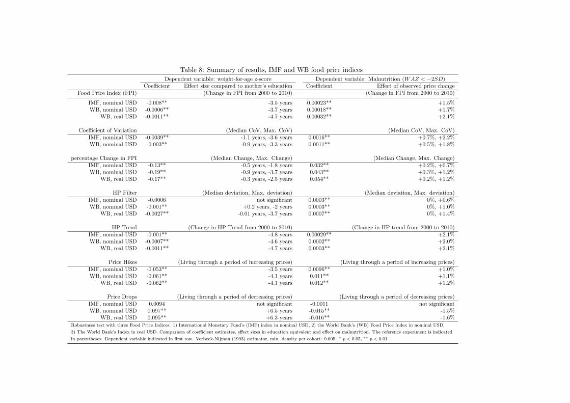
Table 8: Summary of results, IMF and WB food price indices
Dependent variable: weight-for-age z-score Dependent variable: Malnutrition (WAZ < −2SD)Coefficient Effect size compared to mother’s education Coefficient Effect of observed price change
Food Price Index (FPI) (Change in FPI from 2000 to 2010) (Change in FPI from 2000 to 2010)
IMF, nominal USD -0.008** -3.5 years 0.00023** +1.5%WB, nominal USD -0.0006** -3.7 years 0.00018** +1.7%
WB, real USD -0.0011** -4.7 years 0.00032** +2.1%
Coefficient of Variation (Median CoV, Max. CoV) (Median CoV, Max. CoV)IMF, nominal USD -0.0039** -1.1 years, -3.6 years 0.0016** +0.7%, +2.2%WB, nominal USD -0.003** -0.9 years, -3.3 years 0.0011** +0.5%, +1.8%
percentage Change in FPI (Median Change, Max. Change) (Median Change, Max. Change)IMF, nominal USD -0.13** -0.5 years, -1.8 years 0.032** +0.2%, +0.7%WB, nominal USD -0.19** -0.9 years, -3.7 years 0.043** +0.3%, +1.2%
WB, real USD -0.17** -0.3 years, -2.5 years 0.054** +0.2%, +1.2%
HP Filter (Median deviation, Max. deviation) (Median deviation, Max. deviation)IMF, nominal USD -0.0006 not significant 0.0003** 0%, +0.6%WB, nominal USD -0.001** +0.2 years, -2 years 0.0003** 0%, +1.0%
WB, real USD -0.0027** -0.01 years, -3.7 years 0.0007** 0%, +1.4%
HP Trend (Change in HP Trend from 2000 to 2010) (Change in HP trend from 2000 to 2010)IMF, nominal USD -0.001** -4.8 years 0.00029** +2.1%WB, nominal USD -0.0007** -4.6 years 0.0002** +2.0%
WB, real USD -0.0011** -4.7 years 0.0003** +2.1%
Price Hikes (Living through a period of increasing prices) (Living through a period of increasing prices)IMF, nominal USD -0.053** -3.5 years 0.0096** +1.0%WB, nominal USD -0.061** -4.1 years 0.011** +1.1%
WB, real USD -0.062** -4.1 years 0.012** +1.2%
Price Drops (Living through a period of decreasing prices) (Living through a period of decreasing prices)IMF, nominal USD 0.0094 not significant -0.0011 not significantWB, nominal USD 0.097** +6.5 years -0.015** -1.5%
WB, real USD 0.095** +6.3 years -0.016** -1.6%Robustness test with three Food Price Indices: 1) International Monetary Fund’s (IMF) index in nominal USD, 2) the World Bank’s (WB) Food Price Index in nominal USD,
3) The World Bank’s Index in real USD. Comparison of coefficient estimates, effect sizes in education equivalent and effect on malnutrition. The reference experiment is indicated
in parentheses. Dependent variable indicated in first row. Verbeek-Nijman (1993) estimator, min. density per cohort: 0.005. ∗ p < 0.05, ∗∗ p < 0.01.

6.4 Robustness of results to cohort definition
The critical reader may wonder how robust the previous results are with respect to varying the
cohort definition of the synthetic panel. To dispel doubts, I run the models (1) to (7) with WAZ
as dependent variable on various cohort definitions. Cohorts are constructed according to the
procedure described in section 4 whereby the minimum density per cohort is varied from 10 per
cent to 0.25 per cent. This results in synthetic panels with 628 to 5045 observations. Table
13 lists the cohort sizes and corresponding per centiles in the respective synthetic panel. The
results are reported in section 9.2. The coefficient estimates and level of significance prove robust
to varying cohort definitions. In line with the results of the MCS, the standard errors slightly
increase as the number of cohorts decreases.
7 Low on WAZ – where do they live, what are they like?
The previous analysis has demonstrated the economic relevance of the past fluctuation in food
prices. In this section, I will investigate the question of which households are most vulnerable to
adverse effects of food price shocks. In principal, households with under-nourished children (or
with children close to under-nourishment) are most vulnerable in the sense that further deteriora-
tion of their health status can be detrimental. The above statement is exhaustive of the question
under the assumption of homogenous impacts. Obviously, impacts are heterogeneous to some
extent; some possible sources of heterogeneity have been identified in the above discussion of the
literature (e.g. net-seller vs. net-buyers). Even if the impacts of the variation in food prices are
not strictly homogenous, the following descriptive statistics can still provide important insights
on vulnerable households across countries and within countries. The analysis of heterogeneous
impacts of food prices goes beyond the scope of this essay. Some possible avenues for future
research are discussed in the conclusion of this essay.
Tables 9, 30, 31 report descriptive statistics on the weight-for-age score, underweight in
children and severe underweight in children by country. The latter two tables, which contain less
information but enhance easy readability, are reported in the appendix. The descriptive statistics
are weighted by the respective sampling weights of the DHS surveys and are representative of
the situation in the respective country in the most recent year for which data is available.
We can see from the descriptive statistics that underweight is an issue in almost all countries
in the sample. The prevalence of underweight is most pronounced in African countries but
42

is no less severe in some of the Asian countries. In Bangladesh, 50 per cent of children are
underweight and half of those are close to severe underweight. The situation is equally severe in
India, Madagascar, Niger and Chad.
For the Subsaharan countries in the sample, rates of underweight are high ranging from 17
per cent in Rwanda to 49 per cent in Niger. The highest rates of underweight are found in
Burkina Faso (36 per cent), Chad (40 per cent), Ethiopia (39 per cent), Madagascar (48 per
cent), Mozambique (44 per cent) and Niger (49 per cent).
In Asia, underweight is also severe in some countries. The highest rates of underweight are
found in Cambodia (36 per cent), India (55 per cent) and Bangladesh (50 per cent).
In Central and South America, the prevalence of underweight is considerably lower for the
countries in the sample. 8.7 per cent are underweight in Bolivia, 7.6 per cent in Colombia, 7.2
per cent in the Dominican Republic, 12 per cent in Nicaragua, 8 per cent in Peru. Highest rates
of underweight are found in Haiti with 21 per cent and in Guatemala with 31 per cent.
43

Table 9: Weighted descriptive statistics on WAZ by country, sorted by median WAZ.
Country Year Min. 1st Qu. Median Mean s.d. 3rd Qu. Max.
India 2006 -4.998 -3 -2.2 -2.1 1.3 -1.3 4.904Bangladesh 2011 -4.997 -2.8 -2 -1.9 1.3 -1.2 4.81Madagascar 2004 -4.911 -2.8 -1.9 -1.8 1.3 -1.1 4.49
Niger 2006 -4.989 -2.9 -1.9 -1.9 1.4 -0.95 4.664Cambodia 2011 -4.902 -2.3 -1.7 -1.6 1.3 -0.73 2.229
Ethiopia 2003 -4.978 -2.5 -1.7 -1.6 1.4 -0.74 4.456Mozambique 2004 -4.496 -2.5 -1.7 -1.5 1.7 -0.63 3.742
Chad 2004 -4.994 -2.6 -1.6 -1.6 1.6 -0.54 4.677Burkina Faso 2010 -4.998 -2.4 -1.5 -1.6 1.3 -0.73 4.814
Mali 2006 -4.998 -2.5 -1.5 -1.5 1.5 -0.55 4.755Guatemala 1999 -4.894 -2.2 -1.4 -1.4 1.3 -0.57 4.893
Benin 2006 -4.965 -2.1 -1.3 -1.2 1.3 -0.4 4.964Guinea 2005 -4.945 -2.2 -1.3 -1.3 1.5 -0.41 4.749
Lesotho 2010 -4.859 -1.9 -1.3 -1.1 1.4 -0.31 2.739Senegal 2011 -4.877 -2.1 -1.3 -1.3 1.3 -0.55 4.309
Tanzania 2010 -4.96 -2.1 -1.3 -1.3 1.2 -0.49 4.441Kenya 2009 -4.965 -2.1 -1.2 -1.2 1.3 -0.38 3.874
Namibia 2007 -4.978 -2.1 -1.2 -1.2 1.3 -0.34 4.894Nigeria 2008 -4.998 -2.2 -1.2 -1.2 1.6 -0.2 4.964Ghana 2008 -4.989 -1.9 -1.1 -1.1 1.3 -0.26 4.509Malawi 2010 -4.965 -1.9 -1.1 -1.1 1.3 -0.33 4.993Uganda 2011 -4.988 -1.9 -1.1 -1.1 1.3 -0.27 3.64Zambia 2007 -4.968 -1.9 -1.1 -1.1 1.3 -0.31 4.867
Rwanda 2011 -4.76 -1.7 -0.97 -0.94 1.2 -0.19 4.071Zimbabwe 2011 -4.933 -1.7 -0.96 -0.92 1.2 -0.11 4.595
Haiti 2006 -4.929 -1.8 -0.92 -1 1.4 -0.13 3.988Cameroon 2011 -4.988 -1.8 -0.82 -0.89 1.4 0.054 4.49
Morocco 2004 -4.908 -1.5 -0.61 -0.6 1.4 0.29 4.491Nicaragua 2001 -4.924 -1.4 -0.59 -0.58 1.3 0.21 4.97
Bolivia 2008 -4.966 -1.3 -0.52 -0.51 1.2 0.21 4.865Colombia 2010 -4.998 -1.2 -0.51 -0.48 1.1 0.23 4.507
Kazakhstan 1999 -4.464 -1.2 -0.44 -0.45 1.1 0.24 3.042Peru 2008 -4.788 -1.2 -0.44 -0.42 1.2 0.34 4.629
Egypt 2008 -4.914 -1.2 -0.34 -0.34 1.3 0.51 4.994Jordan 2007 -4.96 -1 -0.28 -0.24 1.2 0.53 4.975
Dominican Republic 2007 -4.919 -1 -0.24 -0.23 1.2 0.55 4.957Armenia 2010 -4.402 -0.81 -0.14 -0.14 1.2 0.63 4.224
Turkey 2004 -4.965 -0.88 -0.13 -0.16 1.2 0.58 3.821
44

7.1 More descriptives: socio-economic characteristics
A closer look at the bivariate distributions of WAZ and socio-economic variables can provide
some insights on the characteristics of those cohorts (close to) underweight. Table 10 reports 3D-
density plots of WAZ against the socio-economic variables urban, wealth, female education, male
education, improved water supply, improved sanitation, agriculturally employed and agricultural
self-employed.
The 3D-density plots indicate that cohorts with lower WAZ can rather be found in rural
areas than in urban areas, but the pattern is relatively weak. More pronounced is the bivariate
relation of WAZ with wealth: less wealthy cohorts dispose of a low WAZ and high wealth is also
associated with higher WAZ. Those cohorts with higher male and female education have also
higher WAZ. As for water supply, there seems to be a positive bi-variate association of access
to improved water supply and WAZ. When considering WAZ and improved sanitation, there
appears to be a bi-modal distribution: many cohorts do not dispose of improved sanitation and
have lower values of WAZ and few cohorts have access to improved sanitation which is associated
with higher levels of WAZ. Finally, agricultural employment and self-employment seem to fall
together with low levels of WAZ. Overall, the bivariate 3D-density plots confirm and further
illustrate the results from the multivariate EIV-models regarding the covariates.
7.2 The policy relevance of descriptives
While the multivariate analysis has shown the economic relevance of the recent fluctuation in
food prices and decomposed the variation in prices and its impact on WAZ, the descriptive
analysis in sections 7 and 7.1 can help to identify those who are most in need for public policy
interventions. There is great heterogeneity in WAZ according to regions, countries and socio-
economic characteristics. Malnourishment is especially high in Africa and some countries of
Asia. The descriptive statistics on the socio-economic characteristics can help to identify the
most vulnerable households within countries: These live predominantly in rural areas, many of
them are engaged in agricultural work, possess less assets, have enjoyed less years of education
and have less likely access to improved water and sanitation infrastructure.
45

Table 10: 3D-density plot of WAZ against socio-economic characteristics, based on pseudo panel
Urban
0.0
0.2
0.4
0.6
0.8
1.0
WAZ
−3
−2
−1
0
1
Z
0.0
0.5
1.0
1.5
Wealth
−1
0
1
2
3
4
WAZ
−3
−2
−1
0
1Z
0.0
0.1
0.2
0.3
0.4
Female education in years
0
5
10
15
WAZ
−3
−2
−1
0
1
Z
0.00
0.05
0.10
Male education in years
0
5
10
15
WAZ
−3
−2
−1
0
1
Z
0.00
0.02
0.04
0.06
0.08
0.10
0.12
Improved water supply
0.0
0.2
0.4
0.6
0.8
1.0
WAZ
−3
−2
−1
0
1
Z
0.0
0.2
0.4
0.6
0.8
1.0
1.2
Improved sanitation
0.0
0.2
0.4
0.6
0.8
1.0
WAZ
−3
−2
−1
0
1
Z
0.0
0.5
1.0
1.5
Agricultural employm
ent
0.0
0.5
1.0
1.5
WAZ
−3
−2
−1
0
1
Z
0
2
4
6
Agricultural self−employed
0.0
0.5
1.0
1.5
2.0
WAZ
−3
−2
−1
0
1
Z
0.0
0.2
0.4
0.6

8 Conclusion
The recent surge in food prices and volatility has received much attention from policy makers,
academia, and the general public. In academia, much of the literature on the consequences of
these recent food price hikes focuses on the effect of high food prices in specific regional and
time contexts. This essay contributes to this fast-growing literature by disentangling the effect
of food price variation on household welfare, extending the regional and time perspective, and
by applying a methodology which has not been used to examine this question before.
To attribute the welfare effects to short-, medium- and long-term variation in prices, I de-
compose three food price indices by the International Monetary Fund and the World Bank in
percentage change in prices from one period to the next, a Coefficient of Variation, HP Filter
and Trend, as well as episodes of sustained hikes and drops in prices. To identify the effect of
these price series on household welfare, proxied by the child weight-for-age z-score, I rely on a
pseudo panel approach which allows me to exploit information from repeated cross sections of
the Demographic and Health Surveys on approximately 500,000 children from 38 countries over
a period of 20 years. Instead of following individuals over time as in standard panel approaches,
in this approach, birthyear-cohorts are followed over time. To remedy potential bias due to sam-
pling error, the Verbeek-Nijman (1992) estimator, a variant of the Deaton’s (1985) EIV model,
is applied. This estimator has been shown to perform best in the context of the prevalent data
situation using Monte Carlo Simulation techniques.
I find that increases in the overall food price index have a negative impact on household
welfare. The effect size is economically significant: when compared to the effect size of maternal
education, the observed price increase from the year 2000 to 2010 would offset the positive effect
of 3.5 years of maternal education. It is also illustrative to calculate the effect in terms of child
malnutrition rate (children who fall below a WAZ < −2 SD): the price increase over the same
period leads to a 1.5 per cent increase in the rate of child malnutrition in the countries sampled.
Decomposing the index in the above components, I find that this negative effect operates
through volatility, as measured by the CoV, the change in prices from one period to another,
the HP trend and episodes of sustained increases in prices. The effects can be considered strong
when set in relation to maternal education and malnutrition. The effect of price volatility (CoV)
in the year 2008 on child WAZ corresponds to -3.6 years of maternal education and an increase
in malnutrition by 2.2 per cent. Given that this effect refers to only one year, the effect size can
be considered high. Contrary to the CoV, the impact of the HP Trend materializes over a rather
47
long period of time: the increase in HP Trend from 2000 to 2010 is equivalent to the effect of
-4.8 years of maternal education and translates in an increase of malnutrition by 2.1 per cent.
Living through a period of continued price increases47 corresponds to the effect of -3.5 years of
education or a 1 per cent increase in malnutrition.
There is mixed evidence on the impact of the short-term fluctuation around a trend (HP
Filter) and whether continued decreases in prices improve child health. While the coefficient
estimates based on the IMF’s nominal food price index are insignificant, the estimates based on
the World Bank’s index in both nominal and real terms are significant. According to the latter
results, the variation in the HP Filter has a negative relation with child WAZ: the effect of the
maximum deviation from trend in the year 2008 corresponds to -2 years of maternal education
and implies an increase in malnutrition by 1 per cent. Based on the World Bank data, periods
of subsequent drops in food prices seem to improve child health: the effect size corresponds to
6.5 years of maternal education, or a 1.5 per cent decrease in malnutrition.
To summarize, I find that, overall, there is a negative relationship between the variation in
global food prices and household welfare. The effect is transmitted through short-term price
movements (volatility), medium-term changes (period-to-period change, HP Filter) and perma-
nent shocks to global food prices (HP trend, price hikes). The effects on household welfare are
strong considering equivalent education effects and estimated effects of the above indicators on
malnutrition rates.
Finally, I would like to point to an avenue for future research: the above analysis abstracts
from heterogeneous impacts which go beyond the scope of this essay. Heterogeneous impacts
could be analyzed at different levels of aggregation. At the country level, the status of a country
as a net importer (or exporter) of agricultural goods in relation to total GDP, the pass-through of
international food prices to domestic markets as well as the presence (or absence) of social and
economic institutions could be determinants of impact heterogeneity. At the household level,
factors may include the position of the household as net seller vs. net buyer, wealth, formal
and informal insurance and access to credit. This is by no means an exhaustive list of potential
factors according to which heterogeneous effects may materialize. Detecting impact heterogeneity
at different levels of aggregation, including the country and household level, but potentially also
in-between levels such as regions or districts, is an interesting and important avenue for further
research which could be addressed in the framework of a pseudo panel approach.
47Periods of continued price increases are defined as two or more subsequent upward movements in prices.Periods of sustained drops in prices are defined analogously.
48

9 Appendix
9.1 Results from OLS and Fixed Effects models
Table 11: Ordinary Least-Squares (OLS) Estimator.
(1) (2) (3) (4) (5) (6) (7)
FPI CoV HP Filter HP Trend Price Hike Price Drop PChange
Food Price -0.000419∗∗ 0.0116∗∗ 0.00436∗∗ -0.00145∗∗ 0.0401∗∗ 0.0578∗∗ -0.336∗∗
(0.0000958) (0.000737) (0.000264) (0.000116) (0.00402) (0.00767) (0.0283)
Impr. ws. -0.0424∗∗ -0.0403∗∗ -0.0421∗∗ -0.0420∗∗ -0.0427∗∗ -0.0440∗∗ -0.0439∗∗
(0.00468) (0.00468) (0.00467) (0.00468) (0.00468) (0.00468) (0.00471)
Impr. san. 0.0193∗∗ 0.0218∗∗ 0.0208∗∗ 0.0222∗∗ 0.0228∗∗ 0.0194∗∗ 0.0125∗
(0.00519) (0.00519) (0.00519) (0.00520) (0.00521) (0.00519) (0.00523)
Agr. empl. -0.107∗∗ -0.111∗∗ -0.109∗∗ -0.107∗∗ -0.106∗∗ -0.107∗∗ -0.106∗∗
(0.00457) (0.00458) (0.00458) (0.00457) (0.00457) (0.00457) (0.00463)
Agr. self- 0.0627∗∗ 0.0629∗∗ 0.0651∗∗ 0.0624∗∗ 0.0635∗∗ 0.0643∗∗ 0.0634∗∗
empl. (0.00313) (0.00312) (0.00313) (0.00313) (0.00313) (0.00313) (0.00315)
Wealth 0.124∗∗ 0.125∗∗ 0.125∗∗ 0.123∗∗ 0.125∗∗ 0.125∗∗ 0.125∗∗
(0.00172) (0.00171) (0.00171) (0.00172) (0.00171) (0.00171) (0.00173)
Female educ. 0.0265∗∗ 0.0261∗∗ 0.0261∗∗ 0.0266∗∗ 0.0263∗∗ 0.0263∗∗ 0.0263∗∗
(0.000616) (0.000615) (0.000615) (0.000615) (0.000615) (0.000615) (0.000620)
Urban 0.0411∗∗ 0.0411∗∗ 0.0433∗∗ 0.0415∗∗ 0.0417∗∗ 0.0414∗∗ 0.0405∗∗
(0.00508) (0.00508) (0.00508) (0.00508) (0.00508) (0.00508) (0.00512)
Male educ. 0.0168∗∗ 0.0164∗∗ 0.0166∗∗ 0.0168∗∗ 0.0167∗∗ 0.0168∗∗ 0.0168∗∗
(0.000552) (0.000552) (0.000552) (0.000552) (0.000552) (0.000552) (0.000556)
GDP 0.194∗∗ 0.190∗∗ 0.192∗∗ 0.196∗∗ 0.192∗∗ 0.193∗∗ 0.195∗∗
(0.00252) (0.00251) (0.00251) (0.00251) (0.00251) (0.00251) (0.00253)
Time trend -0.00843∗∗ -0.0130∗∗ -0.0103∗∗ -0.00550∗∗ -0.0104∗∗ -0.00897∗∗ -0.00611∗∗
(0.000464) (0.000417) (0.000363) (0.000493) (0.000367) (0.000374) (0.000471)
Constant -2.514∗∗ -2.533∗∗ -2.520∗∗ -2.452∗∗ -2.535∗∗ -2.545∗∗ -2.570∗∗
(0.0178) (0.0170) (0.0171) (0.0183) (0.0170) (0.0171) (0.0173)
Observations 497839 497839 497839 497839 497839 497839 489965
Dependent variable: Weight-for-age z-score. Standard errors in parentheses.∗ p < 0.05, ∗∗ p < 0.01
OLS estimation
49

Table 12: Efficient Wald / Fixed Effects Estimator.
(1) (2) (3) (4) (5) (6) (7)
FPI CoV HP Filter HP Trend Price Hike Price Drop PChange
Food Price -0.00170∗∗ -0.00905∗∗ -0.000972 -0.00230∗∗ -0.0176 -0.0362∗ -0.0729(0.000275) (0.00241) (0.000791) (0.000331) (0.0115) (0.0184) (0.0654)
Impr. ws. 0.0367 0.0284 0.0187 0.0408 0.0170 0.0210 0.00383(0.0358) (0.0359) (0.0358) (0.0358) (0.0358) (0.0359) (0.0361)
Impr. san. 0.138∗∗ 0.110∗∗ 0.107∗∗ 0.152∗∗ 0.102∗∗ 0.0987∗∗ 0.104∗∗
(0.0367) (0.0365) (0.0366) (0.0369) (0.0368) (0.0369) (0.0369)
Agr. empl. -0.138∗∗ -0.109∗∗ -0.123∗∗ -0.148∗∗ -0.125∗∗ -0.122∗∗ -0.120∗∗
(0.0384) (0.0388) (0.0386) (0.0384) (0.0386) (0.0386) (0.0392)
Agr. self. -0.171∗∗ -0.151∗∗ -0.151∗∗ -0.176∗∗ -0.149∗∗ -0.151∗∗ -0.151∗∗
empl. (0.0251) (0.0249) (0.0250) (0.0251) (0.0250) (0.0250) (0.0252)
Wealth 0.0887∗∗ 0.0949∗∗ 0.0939∗∗ 0.0874∗∗ 0.0927∗∗ 0.0967∗∗ 0.0890∗∗
(0.0188) (0.0188) (0.0188) (0.0187) (0.0189) (0.0189) (0.0191)
Female educ. 0.0240∗∗ 0.0236∗∗ 0.0236∗∗ 0.0239∗∗ 0.0234∗∗ 0.0242∗∗ 0.0264∗∗
(0.00716) (0.00719) (0.00720) (0.00715) (0.00720) (0.00721) (0.00733)
Urban 0.00785 0.0164 0.0160 0.000377 0.0236 -0.000821 0.0317(0.0497) (0.0499) (0.0500) (0.0497) (0.0504) (0.0505) (0.0510)
Male educ. 0.00133 -0.0000827 -0.000821 0.00218 -0.000841 -0.000263 -0.00293(0.00647) (0.00649) (0.00650) (0.00647) (0.00650) (0.00650) (0.00660)
GDP 0.0655 0.0403 0.00873 0.0769 0.00900 0.0175 -0.0169(0.0517) (0.0518) (0.0511) (0.0517) (0.0511) (0.0514) (0.0520)
Time trend 0.00809∗∗ 0.00616∗∗ 0.00461∗∗ 0.00912∗∗ 0.00499∗∗ 0.00371∗ 0.00530∗∗
(0.00152) (0.00148) (0.00142) (0.00155) (0.00145) (0.00147) (0.00157)
Observations 4877 4877 4877 4877 4877 4877 4770
Dependent variable: Weight-for-age z-score. Standard errors in parentheses.∗ p < 0.05, ∗∗ p < 0.01
FE estimation
50

9.2 Robustness: Varying cohort definitions
Table 13: Distribution of cohort size in pseudo panels
per centileMin. Density 5 10 30 50 80 90 95
0.001 4 6 25 55 144 229 3240.0025 4 7 26 56 146 232 3280.005 4 8 28 59 148 235 3340.01 4 9 32 63 154 241 3390.025 5 11 39 76 176 270 3840.05 6 14 55 108 258 385 5420.1 10 25 104 214 514 739 10890.25 18 50 249 511 1214 1770 2549
Table 14: Verbeek-Nijman (1993) Estimator, obs. 5045
(1) (2) (3) (4) (5) (6) (7)
FPI CoV HP Filter HP Trend Price Hike Price Drop PChange
Price Index -0.00076(0.00013)**
-0.0039(0.0011)**
-0.00061(0.00039)
-0.001(0.00016)**
-0.053(0.0058)**
0.011(0.011)
-0.13(0.036)**
Impr. ws. -0.038(0.021)*
-0.041(0.021)*
-0.045(0.021)**
-0.035(0.021)
-0.069(0.021)**
-0.046(0.021)**
-0.049(0.021)**
Impr. san. 0.13(0.02)**
0.12(0.021)**
0.13(0.021)**
0.13(0.02)**
0.09(0.021)**
0.13(0.021)**
0.12(0.021)**
Agr. empl. -0.1(0.024)**
-0.087(0.025)**
-0.096(0.024)**
-0.12(0.024)**
-0.1(0.024)**
-0.1(0.024)**
-0.1(0.024)**
Agr. self-empl. -0.14(0.016)**
-0.12(0.016)**
-0.13(0.016)**
-0.14(0.016)**
-0.12(0.016)**
-0.12(0.016)**
-0.13(0.016)**
Wealth 0.058(0.015)**
0.061(0.015)**
0.061(0.016)**
0.055(0.015)**
0.056(0.015)**
0.058(0.016)**
0.056(0.015)**
Female educ. 0.015(0.0062)**
0.016(0.0062)**
0.016(0.0062)**
0.014(0.0062)**
0.018(0.0061)**
0.015(0.0062)**
0.016(0.0062)**
Urban 0.073(0.041)*
0.084(0.041)**
0.088(0.041)**
0.07(0.041)*
0.13(0.041)**
0.095(0.042)**
0.1(0.041)**
Male educ. 0.023(0.0056)**
0.021(0.0056)**
0.019(0.0056)**
0.024(0.0057)**
0.016(0.0056)**
0.019(0.0056)**
0.02(0.0056)**
GDP 0.094(0.031)**
0.069(0.031)**
0.047(0.03)
0.099(0.031)**
0.057(0.029)*
0.034(0.03)
0.053(0.03)*
Time trend 0.0066(0.00089)**
0.006(0.00088)**
0.0052(0.00086)**
0.0071(0.00091)**
0.0066(0.00087)**
0.0056 (9e-04)**
0.0065(0.00092)**
Observations 5045 5045 5045 5045 5045 5045 4929
Dependent variable: Weight-for-age z-score. Standard errors in parentheses.∗ p < 0.05, ∗∗ p < 0.01
Verbeek-Nijman (1993) estimator, min. density per cohort: 0.001
51

Table 15: Verbeek-Nijman (1993) Estimator, obs. 4979
(1) (2) (3) (4) (5) (6) (7)
FPI CoV HP Filter HP Trend Price Hike Price Drop PChange
Price Index -0.00076(0.00013)**
-0.0039(0.0011)**
-6e-04(0.00039)
-0.001(0.00016)**
-0.053(0.0058)**
0.01(0.011)
-0.13(0.036)**
Impr. ws. -0.038(0.021)*
-0.041(0.021)*
-0.045(0.021)**
-0.035(0.021)
-0.069(0.021)**
-0.046(0.021)**
-0.049(0.021)**
Impr. san. 0.13(0.02)**
0.12(0.021)**
0.13(0.021)**
0.14(0.021)**
0.091(0.021)**
0.13(0.021)**
0.12(0.021)**
Agr. empl. -0.1(0.024)**
-0.086(0.025)**
-0.096(0.025)**
-0.11(0.024)**
-0.1(0.024)**
-0.1(0.024)**
-0.1(0.024)**
Agr. self-empl. -0.14(0.016)**
-0.12(0.016)**
-0.13(0.016)**
-0.14(0.017)**
-0.13(0.016)**
-0.13(0.016)**
-0.13(0.016)**
Wealth 0.058(0.016)**
0.06(0.016)**
0.06(0.016)**
0.054(0.016)**
0.056(0.015)**
0.058(0.016)**
0.056(0.016)**
Female educ. 0.015(0.0062)**
0.016(0.0062)**
0.016(0.0062)**
0.014(0.0062)**
0.018(0.0062)**
0.015(0.0062)**
0.016(0.0062)**
Urban 0.071(0.041)*
0.082(0.041)**
0.086(0.041)**
0.068(0.041)
0.13(0.041)**
0.093(0.042)**
0.1(0.042)**
Male educ. 0.023(0.0057)**
0.022(0.0057)**
0.02(0.0057)**
0.025(0.0057)**
0.017(0.0056)**
0.02(0.0057)**
0.021(0.0057)**
GDP 0.095(0.031)**
0.07(0.031)**
0.047(0.03)
0.1(0.031)**
0.058(0.03)**
0.035(0.03)
0.053(0.03)*
Time trend 0.0066(0.00089)**
0.0059(0.00089)**
0.0052(0.00087)**
0.0071(0.00091)**
0.0065(0.00087)**
0.0055(0.00091)**
0.0064(0.00093)**
Observations 4979 4979 4979 4979 4979 4979 4868
Dependent variable: Weight-for-age z-score. Standard errors in parentheses.∗ p < 0.05, ∗∗ p < 0.01
Verbeek-Nijman (1993) estimator, min. density per cohort: 0.0025
52

Table 16: Verbeek-Nijman (1993) Estimator, obs. 4877
(1) (2) (3) (4) (5) (6) (7)
FPI CoV HP Filter HP Trend Price Hike Price Drop PChange
Price Index -0.00077(0.00013)**
-0.0039(0.0011)**
-6e-04(0.00039)
-0.001(0.00016)**
-0.053(0.0058)**
0.0094(0.011)
-0.13(0.036)**
Impr. ws. -0.039(0.021)*
-0.042(0.021)*
-0.046(0.021)**
-0.035(0.021)
-0.07(0.021)**
-0.046(0.022)**
-0.049(0.021)**
Impr. san. 0.13(0.021)**
0.12(0.021)**
0.13(0.021)**
0.14(0.021)**
0.091(0.021)**
0.13(0.021)**
0.12(0.021)**
Agr. empl. -0.11(0.024)**
-0.087(0.025)**
-0.097(0.025)**
-0.12(0.024)**
-0.1(0.024)**
-0.1(0.025)**
-0.1(0.024)**
Agr. self-empl. -0.14(0.017)**
-0.13(0.016)**
-0.13(0.016)**
-0.15(0.017)**
-0.13(0.016)**
-0.13(0.016)**
-0.13(0.016)**
Wealth 0.059(0.016)**
0.062(0.016)**
0.062(0.016)**
0.056(0.016)**
0.057(0.016)**
0.059(0.016)**
0.058(0.016)**
Female educ. 0.015(0.0062)**
0.016(0.0063)**
0.015(0.0063)**
0.013(0.0062)**
0.017(0.0062)**
0.015(0.0063)**
0.016(0.0063)**
Urban 0.065(0.042)
0.077(0.042)*
0.081(0.042)*
0.062(0.042)
0.12(0.042)**
0.087(0.042)**
0.095(0.042)**
Male educ. 0.024(0.0057)**
0.022(0.0057)**
0.02(0.0057)**
0.025(0.0057)**
0.017(0.0057)**
0.021(0.0057)**
0.021(0.0057)**
GDP 0.095(0.031)**
0.07(0.031)**
0.048(0.03)
0.1(0.031)**
0.058(0.03)**
0.036(0.03)
0.054(0.03)*
Time trend 0.0065(9e-04)**
0.0059(0.00089)**
0.0052(0.00087)**
0.0071(0.00091)**
0.0065(0.00087)**
0.0054(0.00091)**
0.0064(0.00093)**
Observations 4877 4877 4877 4877 4877 4877 4770
Dependent variable: Weight-for-age z-score. Standard errors in parentheses.∗ p < 0.05, ∗∗ p < 0.01
Verbeek-Nijman (1993) estimator, min. density per cohort: 0.005
53

Table 17: Verbeek-Nijman (1993) Estimator, obs. 4674
(1) (2) (3) (4) (5) (6) (7)
FPI CoV HP Filter HP Trend Price Hike Price Drop PChange
Price Index -0.00078(0.00013)**
-0.0039(0.0011)**
-0.0006(0.0004)
-0.001(0.00016)**
-0.053(0.0059)**
0.0087(0.011)
-0.13(0.036)**
Impr. ws. -0.042(0.022)*
-0.045(0.022)**
-0.049(0.022)**
-0.038(0.022)*
-0.073(0.022)**
-0.049(0.022)**
-0.053(0.022)**
Impr. san. 0.13(0.021)**
0.12(0.021)**
0.13(0.021)**
0.14(0.021)**
0.093(0.021)**
0.13(0.021)**
0.13(0.021)**
Agr. empl. -0.11(0.025)**
-0.088(0.025)**
-0.098(0.025)**
-0.12(0.025)**
-0.1(0.025)**
-0.11(0.025)**
-0.1(0.025)**
Agr. self-empl. -0.14(0.017)**
-0.13(0.017)**
-0.13(0.017)**
-0.15(0.017)**
-0.13(0.016)**
-0.13(0.017)**
-0.13(0.017)**
Wealth 0.057(0.016)**
0.06(0.016)**
0.06(0.016)**
0.054(0.016)**
0.055(0.016)**
0.058(0.016)**
0.056(0.016)**
Female educ. 0.013(0.0064)**
0.014(0.0064)**
0.014(0.0064)**
0.012(0.0064)*
0.016(0.0063)**
0.013(0.0064)**
0.014(0.0064)**
Urban 0.071(0.042)*
0.082(0.042)*
0.086(0.042)**
0.068(0.042)
0.13(0.042)**
0.092(0.043)**
0.1(0.042)**
Male educ. 0.026(0.0058)**
0.024(0.0058)**
0.022(0.0058)**
0.028(0.0059)**
0.019(0.0058)**
0.023(0.0058)**
0.023(0.0058)**
GDP 0.097(0.032)**
0.072(0.031)**
0.049(0.031)
0.1(0.031)**
0.059(0.03)**
0.037(0.03)
0.055(0.03)*
Time trend 0.0066(0.00091)**
0.0059(9e-04)**
0.0052(0.00088)**
0.0072(0.00092)**
0.0065(0.00088)**
0.0055(0.00092)**
0.0064(0.00094)**
Observations 4674 4674 4674 4674 4674 4674 4574
Dependent variable: Weight-for-age z-score. Standard errors in parentheses.∗ p < 0.05, ∗∗ p < 0.01
Verbeek-Nijman (1993) estimator, min. density per cohort: 0.01
54

Table 18: Verbeek-Nijman (1993) Estimator, obs. 4060
(1) (2) (3) (4) (5) (6) (7)
FPI CoV HP Filter HP Trend Price Hike Price Drop PChange
Price Index -0.00079(0.00014)**
-0.0039(0.0012)**
-0.00057(0.00041)
-0.0011(0.00017)**
-0.053(0.006)**
0.0072(0.012)
-0.13(0.037)**
Impr. ws. -0.045(0.022)**
-0.048(0.023)**
-0.052(0.023)**
-0.041(0.022)*
-0.076(0.022)**
-0.052(0.023)**
-0.056(0.023)**
Impr. san. 0.14(0.022)**
0.13(0.022)**
0.13(0.022)**
0.14(0.022)**
0.096(0.022)**
0.14(0.022)**
0.13(0.022)**
Agr. empl. -0.11(0.026)**
-0.092(0.026)**
-0.1(0.026)**
-0.12(0.026)**
-0.11(0.025)**
-0.11(0.026)**
-0.11(0.026)**
Agr. self-empl. -0.15(0.017)**
-0.13(0.017)**
-0.13(0.017)**
-0.15(0.017)**
-0.13(0.017)**
-0.13(0.017)**
-0.13(0.017)**
Wealth 0.049(0.017)**
0.052(0.017)**
0.052(0.017)**
0.046(0.017)**
0.047(0.017)**
0.05(0.017)**
0.048(0.017)**
Female educ. 0.014(0.0067)**
0.015(0.0067)**
0.015(0.0067)**
0.013(0.0067)*
0.017(0.0067)**
0.015(0.0067)**
0.015(0.0067)**
Urban 0.067(0.045)
0.078(0.045)*
0.082(0.045)*
0.064(0.044)
0.13(0.044)**
0.087(0.045)*
0.096(0.045)**
Male educ. 0.028(0.0062)**
0.026(0.0062)**
0.024(0.0062)**
0.029(0.0062)**
0.021(0.0062)**
0.024(0.0062)**
0.024(0.0062)**
GDP 0.098(0.032)**
0.072(0.032)**
0.048(0.032)
0.1(0.032)**
0.059(0.031)*
0.038(0.031)
0.054(0.031)*
Time trend 0.0067(0.00094)**
0.006(0.00093)**
0.0053(0.00091)**
0.0073(0.00095)**
0.0066(0.00091)**
0.0055(0.00095)**
0.0065(0.00097)**
Observations 4060 4060 4060 4060 4060 4060 3982
Dependent variable: Weight-for-age z-score. Standard errors in parentheses.∗ p < 0.05, ∗∗ p < 0.01
Verbeek-Nijman (1993) estimator, min. density per cohort: 0.025
55

Table 19: Verbeek-Nijman (1993) Estimator, obs. 2853
(1) (2) (3) (4) (5) (6) (7)
FPI CoV HP Filter HP Trend Price Hike Price Drop PChange
Price Index -0.00082(0.00015)**
-0.004(0.0013)**
-0.00059(0.00045)
-0.0011(0.00018)**
-0.052(0.0066)**
0.0054(0.013)
-0.12(0.041)**
Impr. ws. -0.056(0.025)**
-0.06(0.025)**
-0.065(0.025)**
-0.052(0.025)**
-0.089(0.025)**
-0.065(0.025)**
-0.068(0.025)**
Impr. san. 0.14(0.024)**
0.13(0.024)**
0.14(0.024)**
0.15(0.024)**
0.1(0.024)**
0.14(0.024)**
0.13(0.024)**
Agr. empl. -0.11(0.028)**
-0.086(0.029)**
-0.097(0.029)**
-0.12(0.028)**
-0.1(0.028)**
-0.1(0.029)**
-0.1(0.028)**
Agr. self-empl. -0.15(0.019)**
-0.13(0.019)**
-0.13(0.019)**
-0.16(0.019)**
-0.13(0.019)**
-0.13(0.019)**
-0.14(0.019)**
Wealth 0.05(0.019)**
0.053(0.019)**
0.053(0.019)**
0.046(0.019)**
0.047(0.019)**
0.05(0.02)**
0.048(0.019)**
Female educ. 0.01(0.0079)
0.012(0.0079)
0.012(0.008)
0.0085(0.0079)
0.014(0.0079)*
0.011(0.008)
0.012(0.0079)
Urban 0.059(0.051)
0.072(0.051)
0.077(0.051)
0.056(0.051)
0.13(0.051)**
0.082(0.052)
0.093(0.051)*
Male educ. 0.033(0.0073)**
0.03(0.0073)**
0.028(0.0073)**
0.035(0.0073)**
0.024(0.0072)**
0.029(0.0073)**
0.029(0.0073)**
GDP 0.1(0.035)**
0.075(0.035)**
0.052(0.034)
0.11(0.035)**
0.062(0.034)*
0.042(0.034)
0.058(0.034)*
Time trend 0.0067(0.001)**
0.0059(0.001)**
0.0052(0.001)**
0.0073(0.001)**
0.0066(0.001)**
0.0054(0.001)**
0.0064(0.0011)**
Observations 2853 2853 2853 2853 2853 2853 2803
Dependent variable: Weight-for-age z-score. Standard errors in parentheses.∗ p < 0.05, ∗∗ p < 0.01
Verbeek-Nijman (1993) estimator, min. density per cohort: 0.05
56

Table 20: Verbeek-Nijman (1993) Estimator, obs. 1497
(1) (2) (3) (4) (5) (6) (7)
FPI CoV HP Filter HP Trend Price Hike Price Drop PChange
Price Index -0.00082(0.00018)**
-0.0039(0.0015)**
-6e-04(0.00053)
-0.0011(0.00022)**
-0.052(0.0078)**
0.0053(0.015)
-0.13(0.049)**
Impr. ws. -0.059(0.03)**
-0.064(0.03)**
-0.068(0.03)**
-0.055(0.03)*
-0.094(0.03)**
-0.068(0.03)**
-0.073(0.03)**
Impr. san. 0.15(0.028)**
0.14(0.029)**
0.14(0.029)**
0.15(0.028)**
0.11(0.029)**
0.15(0.029)**
0.14(0.029)**
Agr. empl. -0.12(0.034)**
-0.1(0.035)**
-0.11(0.035)**
-0.13(0.035)**
-0.12(0.034)**
-0.12(0.035)**
-0.12(0.035)**
Agr. self-empl. -0.16(0.024)**
-0.14(0.023)**
-0.14(0.023)**
-0.17(0.024)**
-0.14(0.023)**
-0.14(0.024)**
-0.15(0.023)**
Wealth 0.044(0.025)*
0.048(0.025)*
0.048(0.025)*
0.04(0.025)
0.039(0.025)
0.045(0.026)*
0.041(0.025)
Female educ. 0.014(0.011)
0.016(0.011)
0.017(0.011)
0.011(0.011)
0.02(0.011)*
0.016(0.011)
0.017(0.011)
Urban 0.058(0.064)
0.072(0.065)
0.078(0.065)
0.055(0.064)
0.14(0.064)**
0.084(0.066)
0.097(0.065)
Male educ. 0.031(0.0098)**
0.028(0.0098)**
0.025(0.0098)**
0.034(0.0098)**
0.02(0.0097)**
0.026(0.0098)**
0.026(0.0098)**
GDP 0.1(0.042)**
0.073(0.042)*
0.05(0.041)
0.11(0.042)**
0.061(0.04)
0.04(0.041)
0.056(0.041)
Time trend 0.0068(0.0012)**
0.0061(0.0012)**
0.0054(0.0012)**
0.0075(0.0013)**
0.0068(0.0012)**
0.0056(0.0013)**
0.0066(0.0013)**
Observations 1497 1497 1497 1497 1497 1497 1471
Dependent variable: Weight-for-age z-score. Standard errors in parentheses.∗ p < 0.05, ∗∗ p < 0.01
Verbeek-Nijman (1993) estimator, min. density per cohort: 0.1
57

Table 21: Verbeek-Nijman (1993) Estimator, obs. 628
(1) (2) (3) (4) (5) (6) (7)
FPI CoV HP Filter HP Trend Price Hike Price Drop PChange
Price Index -0.00083(0.00024)**
-0.0035(0.002)*
-0.00066(0.00072)
-0.0011(0.00029)**
-0.051(0.011)**
0.007(0.021)
-0.13(0.066)*
Impr. ws. -0.057(0.041)
-0.062(0.041)
-0.067(0.041)
-0.052(0.041)
-0.093(0.041)**
-0.067(0.041)
-0.072(0.041)*
Impr. san. 0.14(0.039)**
0.13(0.039)**
0.14(0.039)**
0.15(0.039)**
0.1(0.039)**
0.14(0.039)**
0.13(0.039)**
Agr. empl. -0.13(0.047)**
-0.11(0.048)**
-0.12(0.048)**
-0.14(0.047)**
-0.13(0.047)**
-0.13(0.048)**
-0.13(0.047)**
Agr. self-empl. -0.16(0.032)**
-0.14(0.032)**
-0.14(0.032)**
-0.17(0.032)**
-0.14(0.032)**
-0.14(0.032)**
-0.15(0.032)**
Wealth 0.033(0.037)
0.037(0.037)
0.037(0.037)
0.029(0.037)
0.026(0.037)
0.033(0.037)
0.029(0.037)
Female educ. 0.023(0.017)
0.026(0.017)
0.027(0.017)
0.02(0.017)
0.032(0.017)*
0.026(0.017)
0.028(0.017)*
Urban 0.059(0.092)
0.078(0.093)
0.085(0.093)
0.055(0.092)
0.15(0.092)*
0.095(0.094)
0.11(0.093)
Male educ. 0.026(0.014)*
0.022(0.014)
0.018(0.014)
0.03(0.014)**
0.011(0.014)
0.019(0.014)
0.019(0.014)
GDP 0.12(0.057)**
0.085(0.057)
0.065(0.055)
0.12(0.057)**
0.076(0.054)
0.054(0.055)
0.072(0.055)
Time trend 0.0067(0.0017)**
0.0059(0.0016)**
0.0053(0.0016)**
0.0073(0.0017)**
0.0068(0.0016)**
0.0056(0.0017)**
0.0066(0.0017)**
Observations 628 628 628 628 628 628 616
Dependent variable: Weight-for-age z-score. Standard errors in parentheses.∗ p < 0.05, ∗∗ p < 0.01
Verbeek-Nijman (1993) estimator, min. density per cohort: 0.25
58

9.3 Robustness: Estimation of joint specification of HP Filter andTrend (λ = 6.25)
Table 22: Verbeek-Nijman (1993) Estimator, HP Filter and Trend (λ = 6.25)
Estimate S.E. t-value
HP filter 0.00043 0.00042 1HP trend -0.0012 0.00017 -6.9Impr. ws. -0.027 0.021 -1.3Impr. san. 0.14 0.021 6.6Agr. empl. -0.13 0.024 -5.2Agr. self-empl.
-0.15 0.017 -8.9
Wealth 0.06 0.015 3.9Female educ. 0.012 0.0062 1.9Urban 0.049 0.041 1.2Male educ. 0.026 0.0057 4.6GDP 0.12 0.031 3.8Time trend 0.0072 9e-04 8Dep. var.: WAZ, obs. 4877.
59

9.4 Robustness: Re-defining Water Supply
Table 23: Verbeek-Nijman (1993) Estimator, altered WSS definition
(1) (2) (3) (4) (5) (6) (7)
FPI CoV HP Filter HP Trend Price Hike Price Drop PChange
Price Index -0.00085(0.00015)**
-0.0042(0.0013)**
-0.00062(0.00045)
-0.0011(0.00018)**
-0.053(0.0066)**
0.00082(0.013)
-0.12(0.041)**
Basic ws. -0.056(0.026)**
-0.053(0.026)**
-0.055(0.027)**
-0.053(0.026)**
-0.092(0.027)**
-0.052(0.027)*
-0.055(0.027)**
Adv. ws. -0.03(0.041)
-0.028(0.041)
-0.028(0.041)
-0.03(0.041)
-0.033(0.041)
-0.028(0.041)
-0.027(0.041)
Impr. san. 0.14(0.024)**
0.13(0.024)**
0.13(0.024)**
0.15(0.024)**
0.098(0.024)**
0.14(0.024)**
0.13(0.024)**
Agr. empl. -0.11(0.028)**
-0.085(0.029)**
-0.096(0.029)**
-0.12(0.028)**
-0.1(0.028)**
-0.1(0.029)**
-0.1(0.028)**
Agr. self-empl. -0.14(0.019)**
-0.13(0.019)**
-0.13(0.019)**
-0.15(0.019)**
-0.12(0.019)**
-0.13(0.019)**
-0.13(0.019)**
Wealth 0.042(0.021)**
0.045(0.021)**
0.045(0.021)**
0.039(0.021)*
0.032(0.021)
0.044(0.021)**
0.04(0.021)*
Female educ. 0.012(0.008)
0.014(0.008)*
0.014(0.008)*
0.01(0.008)
0.017(0.0079)**
0.013(0.008)
0.014(0.008)*
Urban 0.037(0.054)
0.048(0.055)
0.051(0.055)
0.036(0.054)
0.086(0.054)
0.054(0.055)
0.065(0.055)
Male educ. 0.032(0.0073)**
0.03(0.0073)**
0.027(0.0073)**
0.035(0.0073)**
0.023(0.0072)**
0.028(0.0073)**
0.028(0.0073)**
GDP 0.099(0.035)**
0.07(0.035)**
0.044(0.034)
0.11(0.035)**
0.052(0.033)
0.036(0.034)
0.049(0.034)
Time trend 0.0072(0.0011)**
0.0064(0.0011)**
0.0057(0.0011)**
0.0078(0.0011)**
0.0075(0.0011)**
0.0057(0.0011)**
0.0069(0.0011)**
Observations 4877 4877 4877 4877 4877 4877 4770
Dependent variable: Weight-for-age z-score. Standard errors in parentheses.∗ p < 0.05, ∗∗ p < 0.01
Verbeek-Nijman (1993) estimator, min. density per cohort: 0.005
60

9.5 Robustness: Underweight
Table 24: Food prices and underweight (WAZ < −2SD)
(1) (2) (3) (4) (5) (6) (7)
FPI CoV HP Filter HP Trend Price Hike Price Drop PChange
Price Index 0.00023(3.9e-05)**
0.0016(0.00032)**
3e-04(0.00011)**
0.00029(4.7e-05)**
0.0096(0.0017)**
-0.0011(0.0033)
0.032(0.01)**
Impr. ws. 0.0012(0.0062)
0.0018(0.0062)
0.0035(0.0062)
0.00034(0.0062)
0.0076(0.0063)
0.0033(0.0063)
0.0042(0.0063)
Impr. san. -0.03(0.006)**
-0.026(0.006)**
-0.028(0.006)**
-0.032(0.006)**
-0.023(0.0061)**
-0.03(0.006)**
-0.028(0.006)**
Agr. empl. 0.019(0.0071)**
0.011(0.0072)
0.015(0.0072)**
0.022(0.0071)**
0.018(0.0071)**
0.018(0.0071)**
0.018(0.0071)**
Agr. self-empl. 0.028(0.0048)**
0.023(0.0048)**
0.023(0.0048)**
0.029(0.0048)**
0.023(0.0048)**
0.023(0.0048)**
0.024(0.0048)**
Wealth -0.02(0.0045)**
-0.021(0.0045)**
-0.021(0.0046)**
-0.019(0.0045)**
-0.02(0.0045)**
-0.02(0.0046)**
-0.02(0.0046)**
Female educ. -0.00024(0.0018)
-0.00066(0.0018)
-0.00062(0.0018)
8.8e-05(0.0018)
-0.00074(0.0018)
-3e-04(0.0018)
-0.00052(0.0018)
Urban -0.02(0.012)
-0.023(0.012)*
-0.024(0.012)**
-0.019(0.012)
-0.033(0.012)**
-0.026(0.012)**
-0.028(0.012)**
Male educ. -0.0056(0.0017)**
-0.0052(0.0017)**
-0.0045(0.0017)**
-0.006(0.0017)**
-0.004(0.0017)**
-0.0046(0.0017)**
-0.0047(0.0017)**
GDP -0.032(0.0091)**
-0.028(0.009)**
-0.019(0.0088)**
-0.032(0.0091)**
-0.019(0.0087)**
-0.015(0.0088)*
-0.019(0.0087)**
Time trend -0.0025(0.00026)**
-0.0024(0.00026)**
-0.0021(0.00025)**
-0.0027(0.00027)**
-0.0023(0.00026)**
-0.0021(0.00026)**
-0.0024(0.00027)**
Observations 4877 4877 4877 4877 4877 4877 4770
Dependent variable: Per cent of children underweight. Standard errors in parentheses.∗ p < 0.05, ∗∗ p < 0.01
Verbeek-Nijman (1993) estimator, min. density per cohort: 0.005
61

9.6 Robustness: Severe Underweight
Table 25: Food prices and severe underweight (WAZ < −3SD)
(1) (2) (3) (4) (5) (6) (7)
FPI CoV HP Filter HP Trend Price Hike Price Drop PChange
Price Index 0.00014(2.6e-05)**
0.0012(0.00022)**
4e-04(7.8e-05)**
0.00013(3.2e-05)**
0.0074(0.0012)**
-0.0034(0.0022)
0.027(0.0072)**
Impr. ws. 0.0075(0.0043)*
0.0077(0.0043)*
0.0092(0.0043)**
0.0074(0.0043)*
0.012(0.0043)**
0.009(0.0043)**
0.0096(0.0043)**
Impr. san. -0.011(0.0041)**
-0.0084(0.0041)**
-0.0089(0.0041)**
-0.012(0.0041)**
-0.0058(0.0042)
-0.012(0.0041)**
-0.0098(0.0041)**
Agr. empl. 0.017(0.0049)**
0.011(0.0049)**
0.012(0.0049)**
0.018(0.0049)**
0.016(0.0048)**
0.017(0.0049)**
0.016(0.0049)**
Agr. self-empl. 0.023(0.0033)**
0.021(0.0033)**
0.021(0.0033)**
0.023(0.0033)**
0.021(0.0033)**
0.021(0.0033)**
0.022(0.0033)**
Wealth -0.008(0.0031)**
-0.0087(0.0031)**
-0.0093(0.0031)**
-0.0077(0.0031)**
-0.0078(0.0031)**
-0.0079(0.0031)**
-0.0077(0.0031)**
Female educ. 0.0012(0.0012)
0.00091(0.0012)
0.00075(0.0012)
0.0014(0.0012)
0.00084(0.0012)
0.0012(0.0012)
0.00099(0.0012)
Urban -0.023(0.0083)**
-0.024(0.0083)**
-0.025(0.0083)**
-0.023(0.0083)**
-0.032(0.0083)**
-0.027(0.0084)**
-0.028(0.0083)**
Male educ. -0.003(0.0011)**
-0.0029(0.0011)**
-0.0022(0.0011)**
-0.0031(0.0011)**
-0.002(0.0011)*
-0.0024(0.0011)**
-0.0025(0.0011)**
GDP -0.031(0.0062)**
-0.03(0.0062)**
-0.026(0.006)**
-0.029(0.0062)**
-0.023(0.0059)**
-0.02(0.006)**
-0.024(0.006)**
Time trend -0.0016(0.00018)**
-0.0016(0.00018)**
-0.0013(0.00017)**
-0.0016(0.00018)**
-0.0016(0.00017)**
-0.0015(0.00018)**
-0.0016(0.00018)**
Observations 4877 4877 4877 4877 4877 4877 4770
Dependent variable: Per cent of children severely underweight. Standard errors in parentheses.∗ p < 0.05, ∗∗ p < 0.01
Verbeek-Nijman (1993) estimator, min. density per cohort: 0.005
62

9.7 World Bank’s Food Price Index in nominal USD
Table 26: Verbeek-Nijman (1993) Estimator, dep. var. WAZ, WB FPI in nominal USD.
(1) (2) (3) (4) (5) (6) (7)
FPI CoV HP Filter HP Trend Price Hike Price Drop PChange
Price Index -6e-04(9.9e-05)**
-0.003(0.00088)**
-0.00096(0.00028)**
-0.00068(0.00012)**
-0.061(0.0057)**
0.097(0.007)**
-0.19(0.027)**
Impr. ws. -0.036(0.021)*
-0.041(0.021)*
-0.049(0.021)**
-0.033(0.022)
-0.07(0.021)**
-0.11(0.022)**
-0.058(0.021)**
Impr. san. 0.13(0.021)**
0.12(0.021)**
0.12(0.021)**
0.13(0.021)**
0.085(0.021)**
0.13(0.02)**
0.11(0.021)**
Agr. empl. -0.1(0.024)**
-0.086(0.025)**
-0.084(0.025)**
-0.11(0.024)**
-0.096(0.024)**
-0.11(0.024)**
-0.094(0.024)**
Agr. self-empl. -0.14(0.016)**
-0.12(0.016)**
-0.12(0.016)**
-0.14(0.017)**
-0.12(0.016)**
-0.11(0.016)**
-0.13(0.016)**
Wealth 0.061(0.016)**
0.062(0.016)**
0.066(0.016)**
0.057(0.016)**
0.06(0.015)**
0.053(0.015)**
0.058(0.016)**
Female educ. 0.015(0.0062)**
0.016(0.0063)**
0.017(0.0063)**
0.013(0.0063)**
0.017(0.0062)**
0.012(0.0061)*
0.018(0.0063)**
urban 0.062(0.042)
0.078(0.042)*
0.083(0.042)**
0.059(0.042)
0.12(0.041)**
0.16(0.041)**
0.11(0.042)**
Male educ. 0.024(0.0057)**
0.022(0.0057)**
0.019(0.0057)**
0.025(0.0058)**
0.018(0.0056)**
0.018(0.0056)**
0.02(0.0057)**
GDP 0.098(0.031)**
0.072(0.031)**
0.061(0.03)**
0.091(0.031)**
0.065(0.03)**
0.086(0.029)**
0.083(0.03)**
Time trend 0.0068(9e-04)**
0.0059(0.00089)**
0.0049(0.00087)**
0.0072(0.00093)**
0.0059(0.00086)**
0.0065(0.00086)**
0.0067(0.00089)**
Observations 4877 4877 4877 4877 4877 4877 4770
Dependent variable: Weight-for-age z-score. WB FPI in nominal USD. Standard errors in parentheses.∗ p < 0.05, ∗∗ p < 0.01
Verbeek-Nijman (1993) estimator, min. density per cohort: 0.005
63

Table 27: Verbeek-Nijman (1993) Estimator, dep. var. underweight, WB FPI in nominal USD.
(1) (2) (3) (4) (5) (6) (7)
FPI CoV HP Filter HP Trend Price Hike Price Drop PChange
Price Index 0.00018(2.9e-05)**
0.0011(0.00026)**
0.00031(8e-05)**
2e-04(3.4e-05)**
0.011(0.0017)**
-0.015(0.0021)**
0.043(0.008)**
Impr. ws. 0.00054(0.0062)
0.0017(0.0062)
0.0044(0.0063)
-0.00054(0.0063)
0.0078(0.0063)
0.012(0.0064)**
0.0061(0.0063)
Impr. san. -0.029(0.006)**
-0.026(0.0061)**
-0.026(0.0061)**
-0.031(0.006)**
-0.022(0.0061)**
-0.03(0.006)**
-0.027(0.006)**
Agr. empl. 0.018(0.0071)**
0.012(0.0072)
0.012(0.0073)
0.021(0.0071)**
0.017(0.0071)**
0.02(0.0071)**
0.016(0.0071)**
Agr. self-empl. 0.027(0.0048)**
0.022(0.0048)**
0.022(0.0048)**
0.028(0.0048)**
0.022(0.0048)**
0.022(0.0048)**
0.023(0.0048)**
Wealth -0.021(0.0045)**
-0.021(0.0045)**
-0.022(0.0046)**
-0.02(0.0045)**
-0.021(0.0045)**
-0.019(0.0045)**
-0.02(0.0045)**
Female educ. -3e-04(0.0018)
-0.00059(0.0018)
-0.00092(0.0018)
1e-04(0.0018)
-0.00071(0.0018)
0.00018(0.0018)
-0.00095(0.0018)
urban -0.019(0.012)
-0.023(0.012)*
-0.025(0.012)**
-0.018(0.012)
-0.032(0.012)**
-0.037(0.012)**
-0.03(0.012)**
Male educ. -0.0056(0.0017)**
-0.0052(0.0017)**
-0.0042(0.0017)**
-0.006(0.0017)**
-0.0042(0.0017)**
-0.0043(0.0017)**
-0.0045(0.0017)**
GDP -0.033(0.0091)**
-0.027(0.0091)**
-0.022(0.0088)**
-0.031(0.009)**
-0.02(0.0087)**
-0.022(0.0087)**
-0.025(0.0088)**
Time trend -0.0026(0.00026)**
-0.0024(0.00026)**
-0.002(0.00025)**
-0.0027(0.00027)**
-0.0022(0.00025)**
-0.0023(0.00025)**
-0.0025(0.00026)**
Observations 4877 4877 4877 4877 4877 4877 4770
Dependent variable: Underweight. WB FPI in nominal USD. Standard errors in parentheses.∗ p < 0.05, ∗∗ p < 0.01
Verbeek-Nijman (1993) estimator, min. density per cohort: 0.005
64

9.8 World Bank’s Food Price Index in real USD
Table 28: Verbeek-Nijman (1993) Estimator, dep. var. WAZ, WB FPI in real USD.
(1) (2) (3) (4) (5) (6) (7)
FPI CoV HP Filter HP Trend Price Hike Price Drop PChange
Price Index -0.0011(0.00016)**
-0.003(0.00088)**
-0.0027(4e-04)**
-0.0011(2e-04)**
-0.062(0.0059)**
0.095(0.0071)**
-0.17(0.037)**
Impr. ws. -0.035(0.021)
-0.041(0.021)*
-0.055(0.021)**
-0.032(0.022)
-0.072(0.021)**
-0.11(0.022)**
-0.049(0.021)**
Impr. san. 0.13(0.021)**
0.12(0.021)**
0.11(0.021)**
0.13(0.021)**
0.082(0.021)**
0.13(0.02)**
0.12(0.021)**
Agr. empl. -0.097(0.024)**
-0.086(0.025)**
-0.062(0.025)**
-0.11(0.024)**
-0.098(0.024)**
-0.11(0.024)**
-0.093(0.024)**
Agr. self-empl. -0.14(0.016)**
-0.12(0.016)**
-0.11(0.016)**
-0.14(0.017)**
-0.12(0.016)**
-0.11(0.016)**
-0.12(0.016)**
Wealth 0.062(0.016)**
0.062(0.016)**
0.071(0.016)**
0.057(0.016)**
0.059(0.015)**
0.048(0.015)**
0.061(0.016)**
Female educ. 0.014(0.0062)**
0.016(0.0063)**
0.017(0.0063)**
0.013(0.0063)**
0.017(0.0062)**
0.012(0.0062)**
0.017(0.0063)**
urban 0.056(0.042)
0.078(0.042)*
0.081(0.042)**
0.057(0.042)
0.13(0.041)**
0.17(0.042)**
0.08(0.042)*
Male educ. 0.025(0.0057)**
0.022(0.0057)**
0.019(0.0057)**
0.026(0.0058)**
0.017(0.0057)**
0.018(0.0056)**
0.021(0.0057)**
GDP 0.11(0.031)**
0.072(0.031)**
0.084(0.03)**
0.089(0.031)**
0.048(0.03)
0.074(0.029)**
0.068(0.03)**
Time trend 0.0075(0.00092)**
0.0059(0.00089)**
0.0046(0.00087)**
0.0077(0.00097)**
0.0069(0.00088)**
0.0073(0.00087)**
0.0059(0.00088)**
Observations 4877 4877 4877 4877 4877 4877 4770
Dependent variable: Weight-for-age z-score. WB FPI in real USD. Standard errors in parentheses.∗ p < 0.05, ∗∗ p < 0.01
Verbeek-Nijman (1993) estimator, min. density per cohort: 0.005
65
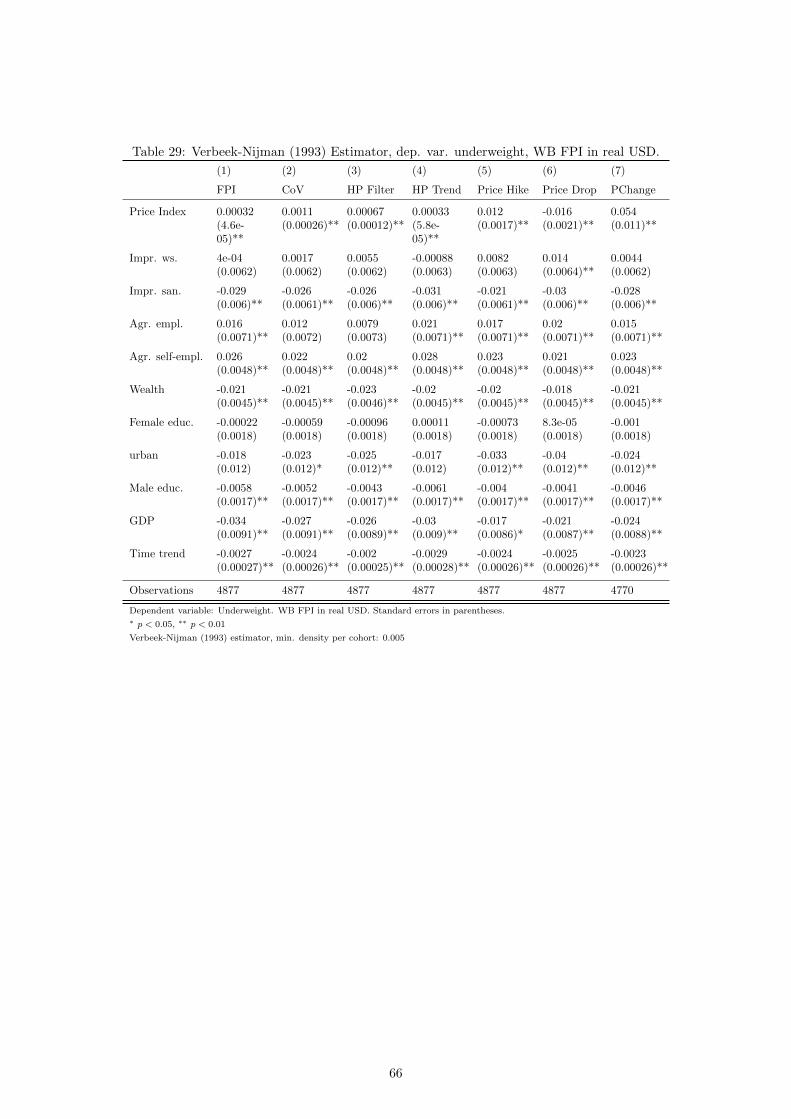
Table 29: Verbeek-Nijman (1993) Estimator, dep. var. underweight, WB FPI in real USD.
(1) (2) (3) (4) (5) (6) (7)
FPI CoV HP Filter HP Trend Price Hike Price Drop PChange
Price Index 0.00032(4.6e-05)**
0.0011(0.00026)**
0.00067(0.00012)**
0.00033(5.8e-05)**
0.012(0.0017)**
-0.016(0.0021)**
0.054(0.011)**
Impr. ws. 4e-04(0.0062)
0.0017(0.0062)
0.0055(0.0062)
-0.00088(0.0063)
0.0082(0.0063)
0.014(0.0064)**
0.0044(0.0062)
Impr. san. -0.029(0.006)**
-0.026(0.0061)**
-0.026(0.006)**
-0.031(0.006)**
-0.021(0.0061)**
-0.03(0.006)**
-0.028(0.006)**
Agr. empl. 0.016(0.0071)**
0.012(0.0072)
0.0079(0.0073)
0.021(0.0071)**
0.017(0.0071)**
0.02(0.0071)**
0.015(0.0071)**
Agr. self-empl. 0.026(0.0048)**
0.022(0.0048)**
0.02(0.0048)**
0.028(0.0048)**
0.023(0.0048)**
0.021(0.0048)**
0.023(0.0048)**
Wealth -0.021(0.0045)**
-0.021(0.0045)**
-0.023(0.0046)**
-0.02(0.0045)**
-0.02(0.0045)**
-0.018(0.0045)**
-0.021(0.0045)**
Female educ. -0.00022(0.0018)
-0.00059(0.0018)
-0.00096(0.0018)
0.00011(0.0018)
-0.00073(0.0018)
8.3e-05(0.0018)
-0.001(0.0018)
urban -0.018(0.012)
-0.023(0.012)*
-0.025(0.012)**
-0.017(0.012)
-0.033(0.012)**
-0.04(0.012)**
-0.024(0.012)**
Male educ. -0.0058(0.0017)**
-0.0052(0.0017)**
-0.0043(0.0017)**
-0.0061(0.0017)**
-0.004(0.0017)**
-0.0041(0.0017)**
-0.0046(0.0017)**
GDP -0.034(0.0091)**
-0.027(0.0091)**
-0.026(0.0089)**
-0.03(0.009)**
-0.017(0.0086)*
-0.021(0.0087)**
-0.024(0.0088)**
Time trend -0.0027(0.00027)**
-0.0024(0.00026)**
-0.002(0.00025)**
-0.0029(0.00028)**
-0.0024(0.00026)**
-0.0025(0.00026)**
-0.0023(0.00026)**
Observations 4877 4877 4877 4877 4877 4877 4770
Dependent variable: Underweight. WB FPI in real USD. Standard errors in parentheses.∗ p < 0.05, ∗∗ p < 0.01
Verbeek-Nijman (1993) estimator, min. density per cohort: 0.005
66

9.9 Descriptive statistics on child underweight by country
Table 30: Weighted descriptive statistics on underweight (pooled cross section)
Country Year Min. 1st Qu. Median Mean s.d. 3rd Qu. Max.
India 2006 0 0 1 0.55 0.5 1 1Bangladesh 2011 0 0 1 0.5 0.5 1 1
Niger 2006 0 0 0 0.49 0.5 1 1Madagascar 2004 0 0 0 0.48 0.5 1 1
Mozambique 2004 0 0 0 0.44 0.51 1 1Chad 2004 0 0 0 0.4 0.49 1 1
Ethiopia 2003 0 0 0 0.39 0.49 1 1Mali 2006 0 0 0 0.37 0.48 1 1
Cambodia 2011 0 0 0 0.36 0.49 1 1Burkina Faso 2010 0 0 0 0.36 0.48 1 1
Guatemala 1999 0 0 0 0.31 0.46 1 1Guinea 2005 0 0 0 0.31 0.46 1 1Nigeria 2008 0 0 0 0.3 0.46 1 1Kenya 2009 0 0 0 0.28 0.45 1 1
Namibia 2007 0 0 0 0.28 0.45 1 1Senegal 2011 0 0 0 0.28 0.45 1 1
Benin 2006 0 0 0 0.27 0.44 1 1Tanzania 2010 0 0 0 0.27 0.44 1 1
Zambia 2007 0 0 0 0.23 0.42 0 1Ghana 2008 0 0 0 0.22 0.42 0 1
Lesotho 2010 0 0 0 0.22 0.42 0 1Malawi 2010 0 0 0 0.22 0.41 0 1Uganda 2011 0 0 0 0.22 0.41 0 1
Cameroon 2011 0 0 0 0.21 0.41 0 1Haiti 2006 0 0 0 0.21 0.41 0 1
Zimbabwe 2011 0 0 0 0.18 0.38 0 1Rwanda 2011 0 0 0 0.17 0.38 0 1Morocco 2004 0 0 0 0.16 0.36 0 1
Nicaragua 2001 0 0 0 0.12 0.33 0 1Egypt 2008 0 0 0 0.1 0.3 0 1
Peru 2008 0 0 0 0.088 0.28 0 1Bolivia 2008 0 0 0 0.087 0.28 0 1
Colombia 2010 0 0 0 0.076 0.27 0 1Dominican Republic 2007 0 0 0 0.072 0.26 0 1
Kazakhstan 1999 0 0 0 0.071 0.26 0 1Jordan 2007 0 0 0 0.068 0.25 0 1
Armenia 2010 0 0 0 0.066 0.25 0 1Turkey 2004 0 0 0 0.06 0.24 0 1
67

Table 31: Weighted descriptive statistics on severe underweight (pooled cross section)
Country Year Min. 1st Qu. Median Mean s.d. 3rd Qu. Max.
India 2006 0 0 0 0.26 0.44 1 1Niger 2006 0 0 0 0.22 0.41 0 1
Bangladesh 2011 0 0 0 0.2 0.4 0 1Madagascar 2004 0 0 0 0.2 0.4 0 1
Mozambique 2004 0 0 0 0.19 0.4 0 1Chad 2004 0 0 0 0.17 0.38 0 1
Cambodia 2011 0 0 0 0.15 0.37 0 1Ethiopia 2003 0 0 0 0.15 0.36 0 1
Mali 2006 0 0 0 0.15 0.36 0 1Burkina Faso 2010 0 0 0 0.14 0.35 0 1
Nigeria 2008 0 0 0 0.13 0.34 0 1Guinea 2005 0 0 0 0.12 0.33 0 1
Lesotho 2010 0 0 0 0.1 0.3 0 1Senegal 2011 0 0 0 0.098 0.3 0 1
Guatemala 1999 0 0 0 0.093 0.29 0 1Benin 2006 0 0 0 0.088 0.28 0 1Kenya 2009 0 0 0 0.087 0.28 0 1
Cameroon 2011 0 0 0 0.08 0.27 0 1Tanzania 2010 0 0 0 0.08 0.27 0 1
Haiti 2006 0 0 0 0.076 0.27 0 1Namibia 2007 0 0 0 0.074 0.26 0 1
Ghana 2008 0 0 0 0.068 0.25 0 1Zambia 2007 0 0 0 0.066 0.25 0 1Uganda 2011 0 0 0 0.064 0.24 0 1Malawi 2010 0 0 0 0.054 0.23 0 1
Morocco 2004 0 0 0 0.054 0.23 0 1Rwanda 2011 0 0 0 0.038 0.19 0 1
Zimbabwe 2011 0 0 0 0.036 0.19 0 1Nicaragua 2001 0 0 0 0.032 0.18 0 1
Egypt 2008 0 0 0 0.026 0.16 0 1Armenia 2010 0 0 0 0.019 0.14 0 1
Bolivia 2008 0 0 0 0.019 0.14 0 1Jordan 2007 0 0 0 0.016 0.12 0 1
Peru 2008 0 0 0 0.015 0.12 0 1Dominican Republic 2007 0 0 0 0.014 0.12 0 1
Turkey 2004 0 0 0 0.014 0.12 0 1Kazakhstan 1999 0 0 0 0.013 0.11 0 1
Colombia 2010 0 0 0 0.012 0.11 0 1
68

9.10 Monte Carlo Simulation
In this appendix, I explore how errors-in-variables (EIV) estimators perform compared to an
OLS and a (Cohort) Fixed Effects Estimator48 in the presence and absence of measurement
error and under alternative cohort definitions. This appendix should be read together with
the identification chapter of this paper which gives a detailed description of the implemented
estimators. Two sets of simulations are run. The first situation corresponds to the typical data
availability of DHS data for one country (2,500 observations per cross section, 4 repeated cross
sections available) and the second mimics the data availability when pooling all DHS data of
countries for which several repeated cross sections are available (approx. 500,000 observations in
total).
Data generating process and definitions
In modeling a synthetic panel (or pseudo panel), I build on Devereux’s (2007a) grouping model
and adapt the data generating process (DGP) to allow for individual and cohort effects. The
variation in the dependent variable xict can be decomposed in cohort variation var(fct) and
individual variation var(vict) around a cohort mean. The former cohort variation can be further
decomposed in variation between cohorts var(fc) and variation within cohorts over time var(ft).
It is the latter variation, the within-cohort-variation, through which coefficients are identified
in the pseudo panel analysis. In the simulation results, I will report the ratio of the within
to total cohort variation(WV =
σftσft+σfc
). Sampling error in the cohort model occurs due
to the individual variation around a cohort mean. Hence, the variance of vict together with
the individual specific variation in κi, in relation to overall variance in xict determines the
strength of the measurement error problem; a metric of the sampling variance is reported as
ICV =σvict+σκiσxict
. The DGP is then specified as follows:
xict = fc + ft + κi + vict (19)
yict = β0 + β1(fc + ft) + hc + λi + uict (20)
Where feasible, the same definitions and parameter choices as in Devereux (2007a) were
48Angrist (1991); Devereux (2007b) refer to this estimator as efficient Wald estimator.
69

implemented to ensure the comparability of results. The constant of the model β0 is set to zero
and β1 is set equal to one. The random variables fc, ft, hc, κi, λi, vict and uict are drawn from
a multivariate or univariate normal distribution respectively according to the specification in
below equations.
In the identification chapter of this paper, it was discussed that the child health outcomes
are likely to be determined in part by unobserved time-invariant household characteristics which
may be correlated with observed household characteristics of the model. For this reason, I
introduce individual and cohort effects to this analysis. The individual and cohort effects can be
manipulated in the Monte Carlo Simulation through the parameters σIE and σCE which reflect
the covariances defined below.
fchc
= N
0; σfc σCE
0; σCE 1
(21)
victuict
= N
0; σvict 0
0; 0 1
(22)
κiλi
= N
0; σκi σIE
0; σIE σλi
(23)
ft = N(0;σft) (24)
The following parameter choices are used throughout the simulations. When parameters are
varied to explore properties of the estimators, the values are indicated directly in the tables for
the respective simulation.
70

Parameter choices in the base specificationReplications 100Cohort size I
Nr. of cohorts CTime periods T
E(fc) 0var(fc) 1E(ft) 0
var(ft) 1E(hc) 0
var(hc) 1E(κi) 0
var(κi) 0E(λi) 0
var(λi) 0E(vict) 0
var(vict) 2E(uict) 0
var(uict) 1σIE 0σCE 0
Individual to cohort variation: ICVWithin to total cohort variation WV
Alongside an OLS and a (Cohort) Fixed Effects estimator, three errors-in-variables estima-
tors are run on the artificially generated data. Among the EIV estimators, the Deaton estimator
is implemented with two slightly different approaches for the calculation of standard errors. In-
ference of the first estimator is based on a simplification assumption (see identification chapter);
the second approach uses the exact equation to estimate standard errors. We will see that the
simplification assumption does not lead to different inferences. Devereux (2007a) suggested a
variant of Deaton’s EIV model which is approximately unbiased when only few cohorts can be
defined. In his simulations (which was based on a DGP which generates only few cohorts), this
adjusted estimator outperforms the alternatives. In our case, numerous cohorts can be defined
from the DHS data but the number of repeated cross sections per country is rather limited.
We know from econometric theory (Deaton, 1985; Verbeek and Nijman, 1992), that this can
also results in biased estimates for Deaton’s EIV estimator (see identification chapter). For this
reason, I implement Verbeek and Nijman’s (1992) estimator which corrects for biases emerging
from the availability of few pseudo panel rounds.
To summarize, the following estimators are tested on the artificially generated data:
• Ordinary Least Squares
• Fixed Effects Model (with cohort fixed effects), also known as Efficient Wald Estimator
71

• Deaton (1985) estimator with the assumption of known measurement error variances
• Deaton (1985) estimator with the assumption of estimated measurement error variances
• The Verbeek-Nijman (1993) estimator which corrects for a low availability of repeated cross
sections per country
Interpretation of simulation results
The results of the Monte Carlo Simulation make an impressive case for the application of the
Verbeek-Nijman estimator. The Verbeek-Nijman estimator clearly outperforms the OLS, Fixed
Effects and Deaton estimators under the applied parameter choices. In all scenarios, the Verbeek-
Nijman estimator performs better in terms of bias and random mean squared error than the other
estimators. The comparison between the Fixed Effects estimator and the Deaton estimator is
less clear: In most instances, the Deaton estimator performs better but in some instances the
Fixed Effects estimator shows better performance in terms of RMSE. In any case, OLS is clearly
biased and any of the other three estimators should be preferred to estimating an OLS model
on the pooled cross sections. Furthermore, the Verbeek-Nijman approach also estimates the
standard error accurately, with a tendency to slightly over-estimate the standard errors. The
FE and Deaton estimators considerably under-estimate the true standard error of the estimator
in the presence of measurement error – sometimes by a factor of 15. This is a major flaw for
inference based on these estimators.
Overall, the results are in line with expectations. Sampling errors can lead to substantial
bias in both the small and large sample cases when cohort size is not very large (nc > 2000).
Not surprisingly, the FE and EIV-estimators perform increasingly well with increasing number of
cohorts (increased efficiency), increasing cohort size (more precise estimates of cohort mean) and
increasing panel rounds (increased efficiency). This applies to the small and large sample cases.
In particular, the performance of the EIV estimators increases with I and C when cohort size is
still low. Once, a sufficient number of individuals per cohort is reached, the performance of the
EIV estimators does not change greatly. However, increases in the number of pseudo individuals
(i.e. cohorts) slightly decrease the standard errors and enhance efficiency. For this reason, in
the empirical analysis of this paper, I choose a cohort definition which ensures that cohort size
is above this threshold (approx. nc ≥ 50) and maximizes the number of pseudo individuals.
Another result with great practical relevance for this paper is that the errors-in-variables
72

estimators also perform well in an unbalanced panel set-up. In the unbalanced case, 50 per
cent of the pseudo individuals are sampled in double as many rounds as the remaining pseudo
individuals. The properties of the estimator seem to be similar as in the balanced case. In fact,
the performance of the estimators is enhanced due to the larger amount of available information
(33 per cent more observations).
In the empirical part of this paper, a pseudo panel was constructed based on DHS survey data
and macro-economic data from the World Bank and International Monetary Fund. The pseudo
panel is likely to suffer from measurement error to an extent that warrants the application of an
EIV model. The Monte Carlo simulations show that EIV models perform better compared to
Ordinary Least Squares and Fixed Effects models. Within the class of EIV models, the Verbeek-
Nijman estimator, a version of the Deaton estimator adapted for situations in which only few
repeated cross sections per country are available, seems to outperform its parent. The main
result is in line with Devereux (2007a) who also found that an adapted version49 of the Deaton
estimator outperforms the Fixed Effects model in a situation where only few cohorts could be
defined.
Monte Carlo Simulation with 10,000 observations
In this section, I present the results of Monte Carlo simulations for a situation in which four
repeated cross sections with 2,500 observations each are available. This scenario corresponds
to the typical availability of household survey data (e.g. DHS, LSMS) for many developing
countries.
Basic specification
In this base specification of the MC simulation, I follow Devereux’s (2007a) parameter choices as
close as possible. The results of this exercise are in line with Devereux’s (2007a) findings. The
Verbeek-Nijman estimator outperforms both the Fixed Effects estimator and Deaton’s EIV esti-
mator. The OLS estimator is strongly biased even in the absence of cohort and individual effects.
When applying Devereux’s (2007a) parameter choices, the Fixed Effects estimator outperforms
Deaton’s EIV-estimator which over-corrects the sampling error.
From the base scenario, we can also make an important observation regarding the estimated
49Devereux (2007a) suggests an estimator for situation in which only few cohorts are available.
73

and actual standard errors of the estimators which will carry throughout most of the simulation
runs: The Verbeek-Nijman approach yields adequate standard errors, with a tendency to slightly
over-estimate the standard error – making inference more conservative. Contrarily OLS, FE and
Deaton estimators considerably under-estimate the true standard error of the estimator.
OLS Fixed Effects Deaton(kME) Deaton(eME) Verbeek-Nijman
mean 0.46 0.92 1.10 1.10 1.00est. s.e. 0.01 0.02 0.13 0.13 0.05true s.e. 0.09 0.11 0.53 0.53 0.04
bias 0.54 0.08 0.08 0.08 0.00rmse 0.38 0.12 0.53 0.53 0.04
Total obs.: 10000, true beta: 1, r: 100, I: 50, C: 50, T: 4, ICV: 0.54, WV: 0.39,IE, cor(x,l+u): 0, CE, cor(x,h+u): 0.02.
Varying measurement error in X
In this scenario, I introduce moderate cohort effects and stepwise increase the variance of vict,
the source of sampling or measurement error. In the first simulation, the sampling error is
set to zero. ICV reports the ratio of the individual variation around the cohort mean to total
variation in the dependent variable. In the absence of measurement error, the FE estimator
and the EIV estimators deliver identical results. OLS is biased due to the cohort effects. With
increasing variance in vict, the FE estimator becomes increasingly biased while the Verbeek-
Nijman estimator remains unbiased. With high levels of measurement error, the Deaton estimator
also becomes biased but still outperforms the FE estimator in terms of mean bias but not root
mean squared error. The RMSE of the EIV estimators become large at very high levels of
measurement error.
74

Experiment 1: Varying the strength of measurement error in Xvar(vict), ICV 0,0 1, 0.38 5, 0.74 10, 0.86 25, 0.94 50, 0.97
BIASOLS 0.25 0.24 0.68 0.83 0.92 0.96
Fixed Effects 0.00 0.04 0.15 0.26 0.44 0.57Deaton (kME) 0.00 0.02 0.21 0.18 0.08 0.12Deaton (eME) 0.00 0.02 0.21 0.18 0.08 0.12
Verbeek-Nijman 0.00 0.00 0.00 0.01 0.01 0.16
RMSEOLS 0.18 0.14 0.53 0.72 0.87 0.93
Fixed Effects 0.02 0.07 0.18 0.25 0.39 0.53Deaton (kME) 0.02 0.12 1.70 1.20 2.50 3.00Deaton (eME) 0.02 0.12 1.70 1.20 2.50 3.00
Verbeek-Nijman 0.02 0.04 0.05 0.21 0.28 1.60
σest − σtrueOLS -0.11 -0.07 -0.06 -0.04 -0.02 -0.01
Fixed Effects 0.00 -0.04 -0.13 -0.15 -0.16 -0.17Deaton (kME) -0.01 -0.09 -0.40 -0.61 -0.10 0.80Deaton (eME) -0.01 -0.09 -0.40 -0.60 0.00 0.80
Verbeek-Nijman -0.01 -0.02 0.06 -0.05 0.09 -0.97
Total obs.: 10000, r: 100, I: 50, C: 50, T: 4, WV: 0.38,IE, cor(x,l+u): 0, CE, cor(x,h+u): 0.39
Increasing cohort size
In this scenario, cohort size (i.e. individuals per cohort) are increased stepwise from 5 to 500.
At very low cohort sizes, considerable bias can be noticed in the FE and EIV estimators. As
expected, OLS is even more biased. With increasing cohort size, the bias of the EIV estimator
disappears quickly – the Verbeek-Nijman estimator already performs well at a cohort size of 15
– and less quickly for the FE estimator which is still biased by approximately 10 per cent at a
cohort size of 100.
75

Experiment 2: Increasing Cohort Size (I)Cohort Size (I) 5 15 30 50 100 200 500
Total obs. 1000 3000 6000 10000 20000 40000 100000
BIASOLS 0.67 0.69 0.68 0.70 0.69 0.70 0.68
Fixed Effects 0.52 0.33 0.21 0.16 0.09 0.06 0.02Deaton (kME) 0.22 0.34 0.09 0.11 0.05 0.02 0.00Deaton (eME) 0.22 0.34 0.09 0.11 0.05 0.02 0.00
Verbeek-Nijman 0.21 0.03 0.00 0.01 0.00 0.00 0.01
RMSEOLS 0.53 0.53 0.53 0.54 0.54 0.56 0.53
Fixed Effects 0.47 0.29 0.19 0.17 0.09 0.08 0.02Deaton (kME) 2.90 1.50 0.44 0.29 0.15 0.08 0.01Deaton (eME) 2.90 1.50 0.44 0.29 0.15 0.08 0.01
Verbeek-Nijman 0.26 0.12 0.09 0.09 0.04 0.02 0.01
σest − σtrueOLS -0.05 -0.05 -0.05 -0.05 -0.06 -0.07 -0.07
Fixed Effects -0.15 -0.14 -0.12 -0.12 -0.06 -0.06 -0.01Deaton (kME) -0.10 -0.44 -0.29 -0.18 -0.10 -0.06 0.00Deaton (eME) 0.20 -0.40 -0.29 -0.18 -0.10 -0.06 0.00
Verbeek-Nijman 0.12 0.09 -0.02 -0.03 -0.01 0.00 0.00
R: 100, C: 50, T: 4, ICV: 0.75, WV: 0.4, IE, cor(x,l+u): 0,CE, cor(x,h+u): 0.4
Increasing number of cohorts
In this scenario, the number of pseudo individuals or cohorts is increased stepwise from 5 to 500.
The FE and EIV estimators are biased when there are few cohorts. The EIV estimators become
increasingly unbiased and more efficient with increasing number of cohorts. The same can be
observed for the FE estimator, but the decrease occurs at a lower rate. The OLS results remain
strongly biased throughout all simulations. Unless, the number of cohorts is low (< 50), the
Verbeek-Nijman estimator dominates the others in terms of bias and RMSE.
76

Experiment 3: Increasing the nr. of cohorts (C)Nr. of cohorts (C) 5 15 50 100 500
Total obs. 1000 3000 10000 20000 100000
BIASOLS 0.72 0.71 0.70 0.68 0.69
Fixed Effects 0.14 0.17 0.18 0.14 0.15Deaton (kME) 0.34 0.14 0.12 0.06 0.09Deaton (eME) 0.34 0.14 0.12 0.06 0.09
Verbeek-Nijman 0.06 0.06 0.01 0.01 0.01
RMSEOLS 0.65 0.59 0.56 0.54 0.53
Fixed Effects 0.19 0.18 0.19 0.14 0.14Deaton (kME) 2.20 1.50 0.64 0.15 0.24Deaton (eME) 2.20 1.50 0.64 0.15 0.24
Verbeek-Nijman 0.20 0.43 0.06 0.05 0.02
σest − σtrueOLS -0.10 -0.07 -0.06 -0.07 -0.05
Fixed Effects -0.07 -0.09 -0.13 -0.10 -0.11Deaton (kME) 2.90 -0.40 -0.39 -0.11 -0.21Deaton (eME) 2.90 -0.40 -0.39 -0.11 -0.21
Verbeek-Nijman 0.23 -0.19 0.02 -0.02 0.00
r: 100, I: 50, T: 4, ICV: 0.75, , WV: 0.37,IE, cor(x,l+u): 0, CE, cor(x,h+u): 0.39
Increasing number of rounds
In this scenario, the number of available cross sections is increased from 2 to 32. As intended, the
Verbeek-Nijman estimator, which corrects for a small number of panel rounds, performs already
well with few available rounds and maintains the best performance. The Deaton estimators
perform poorly on two cross sections and increasingly loose their bias thereafter. However, with
four rounds of cross section at disposal, the Deaton estimators are still substantially biased and
perform worse than the Fixed Effects estimator. The Fixed Effects estimator is biased throughout
all simulations but also looses increasingly its bias with increasing rounds, however, less rapidly
than the Deaton estimator which outperforms the FE when many repeated cross sections are
available. The OLS is always strongly biased.
77

Experiment 4: Increasing the number of rounds (T)T, WV 2, 0.23 4, 0.37 8, 0.44 16, 0.47 32, 0.5
BIASOLS 0.73 0.70 0.68 0.67 0.66
Fixed Effects 0.33 0.17 0.12 0.07 0.06Deaton (kME) 11.00 0.42 0.01 0.04 0.04Deaton (eME) 11.00 0.42 0.01 0.04 0.04
Verbeek-Nijman 0.15 0.00 0.01 0.02 0.03
RMSEOLS 0.60 0.55 0.52 0.49 0.48
Fixed Effects 0.42 0.17 0.09 0.03 0.03Deaton (kME) 220.00 3.60 0.04 0.05 0.05Deaton (eME) 220.00 3.60 0.04 0.05 0.05
Verbeek-Nijman 2.10 0.10 0.02 0.05 0.05
σest − σtrueOLS -0.06 -0.05 -0.05 -0.04 -0.62
Fixed Effects -0.25 -0.11 -0.06 -0.01 -0.03Deaton (kME) 2790.00 -0.30 -0.01 -0.03 0.01Deaton (eME) 2890.00 -0.30 -0.01 -0.03 0.01
Verbeek-Nijman 0.20 0.07 0.00 -0.03 0.02
r: 100, I: 50, C: 50, ICV: 0.75,IE, cor(x,l+u): 0, CE, cor(x,h+u): 0.39,
Increasing individual effects
In this scenario, the strength of the individual effect is increased progressively by varying σIE .
The resulting correlation between the dependent variable and the error term is reported in the
table as IE, cor(x,l+u). Overall, the Verbeek-Nijman estimator performs best in terms of bias,
followed by the Deaton estimators and the FE estimator, in this order. As expected, all three
estimators are unaffected (on average) by increases in the strength of the individual effect but it
seems that some adverse realizations of the DGP lead to high RMSE in the EIV estimators at
times. OLS is biased in all simulations. Interestingly, the OLS bias is reduced with increasing
individual effects, but remains at high levels. This strange effect can be explained through the
fact that the bias due to the individual effects has the opposite sign to the attenuation bias and,
therefore, drives the estimate towards the true value.
78

Experiment 5: Increasing the individual effects (IE)cor(x,l+u) 0 0.2 0.4 0.6 0.8 1
BIASOLS 0.78 0.76 0.73 0.71 0.67 0.66
Fixed Effects 0.17 0.16 0.15 0.18 0.15 0.19Deaton (kME) 0.08 0.08 0.14 0.02 0.08 0.09Deaton (eME) 0.08 0.08 0.14 0.02 0.08 0.09
Verbeek-Nijman 0.03 0.07 0.05 0.02 0.31 0.00
RMSEOLS 0.67 0.63 0.59 0.56 0.51 0.48
Fixed Effects 0.20 0.18 0.15 0.20 0.16 0.21Deaton (kME) 1.80 0.36 0.49 0.74 0.17 1.10Deaton (eME) 1.80 0.36 0.49 0.74 0.17 1.10
Verbeek-Nijman 0.19 1.20 0.31 0.16 3.20 0.12
σest − σtrueOLS -0.05 -0.05 -0.05 -0.05 -0.05 -0.04
Fixed Effects -0.14 -0.12 -0.09 -0.14 -0.11 -0.14Deaton (kME) -0.99 -0.27 -0.35 -0.51 -0.10 -0.58Deaton (eME) -0.98 -0.27 -0.34 -0.51 -0.09 -0.57
Verbeek-Nijman -0.05 -1.10 -0.23 -0.07 -2.96 0.01
Total obs.: 10000, r: 100, I: 50, C: 50, T: 4, WV: 0.36,ICV: 0.79, CE, cor(x,h+u): 0.0
Increasing cohort effects
In this scenario, the strength of the cohort effects are progressively increased by varying σCE .
The resulting correlation between the dependent variable and the error term is reported as CE,
cor(x,h+u). The increase in the cohort effect does not considerably affect the performance of
the FE and the EIV estimators. The OLS is increasingly upwards biased which counteracts the
attenuation bias and drives the estimator towards the true value.
79

Experiment 6: Increasing the cohort effects (CE)cor(x,h+u) 0 0.2 0.4 0.6 0.8 1
BIASOLS 0.74 0.72 0.70 0.65 0.64 0.60
Fixed Effects 0.15 0.17 0.16 0.14 0.16 0.13Deaton (kME) 0.11 0.04 0.12 0.06 0.03 0.16Deaton (eME) 0.11 0.04 0.12 0.06 0.03 0.16
Verbeek-Nijman 0.00 0.01 0.00 0.04 0.01 0.00
RMSEOLS 0.62 0.59 0.54 0.49 0.47 0.43
Fixed Effects 0.16 0.20 0.13 0.16 0.16 0.14Deaton (kME) 0.21 0.34 0.46 0.21 0.76 0.93Deaton (eME) 0.21 0.34 0.46 0.21 0.76 0.93
Verbeek-Nijman 0.07 0.07 0.07 0.35 0.16 0.06
σest − σtrueOLS -0.06 -0.07 -0.05 -0.06 -0.06 -0.06
Fixed Effects -0.10 -0.14 -0.08 -0.11 -0.11 -0.10Deaton (kME) -0.13 -0.26 -0.34 -0.15 -0.60 -0.59Deaton (eME) -0.13 -0.26 -0.34 -0.14 -0.60 -0.58
Verbeek-Nijman -0.02 -0.01 -0.01 -0.30 -0.08 0.01
Total obs.: 10000, r: 100, I: 50, C: 50, T: 4, WV: 0.36,ICV: 0.79, IE, cor(x,l+u): 0.0
Increasing individual and cohort effects
In this scenario, the strength of the individual and cohort effects are progressively increased by
varying σIE and σCE simultaneously. The resulting correlation between the dependent variable
and the error term plus the individual and cohort effect respectively is reported as IE, cor(x,h+u)
and CE, cor(x,h+u). By construction, the two metrics do not report the total correlation between
the dependent variable and the error term, but only with the error term uict plus either the
individual λi or cohort effect hc which are subsumed in the error term respectively. As in
previous scenarios, the increase in the individual and cohort effects, on average, does not affect
the FE and the EIV estimators but adverse realizations of the DGP can lead to higher RMSE.
The OLS is increasingly upward-biased which counteracts the attenuation bias and drives the
estimator towards the true value.
80

Experiment 7: Increasing indiv. and cohort effects (ICE)cor(x,h+l), cor(x,h+u) 0 0.2 0.4 0.6 0.8 1
BIASOLS 0.79 0.74 0.68 0.63 0.57 0.52
Fixed Effects 0.16 0.18 0.17 0.15 0.16 0.16Deaton (kME) 0.29 0.48 0.12 0.16 0.14 0.09Deaton (eME) 0.29 0.48 0.12 0.16 0.14 0.09
Verbeek-Nijman 0.07 0.32 0.04 0.03 0.18 0.05
RMSEOLS 0.68 0.60 0.52 0.46 0.38 0.33
Fixed Effects 0.15 0.20 0.17 0.16 0.17 0.19Deaton (kME) 1.40 6.90 0.49 0.68 0.67 0.73Deaton (eME) 1.40 6.90 0.49 0.68 0.67 0.73
Verbeek-Nijman 0.18 2.50 0.38 0.11 1.80 0.65
σest − σtrueOLS -0.05 -0.05 -0.05 -0.05 -0.05 -0.05
Fixed Effects -0.10 -0.13 -0.11 -0.11 -0.12 -0.13Deaton (kME) -0.82 5.40 -0.35 -0.49 -0.39 -0.44Deaton (eME) -0.81 6.40 -0.35 -0.49 -0.38 -0.43
Verbeek-Nijman -0.06 -2.01 -0.30 -0.04 -1.66 -0.53
Total obs.: 10000, r: 100, I: 50, C: 50, T: 4, WV: 0.35,ICV: 0.79
Unbalanced panel: Increasing measurement error in X
In this scenario, an unbalanced panel is simulated. 50 per cent of the pseudo individuals are
sampled in double as many rounds as the remaining pseudo individuals. For this reason, the
number of observations is increased by 33 per cent. As in a previous scenario, the variance of
vict is progressively increased which enhances the measurement error problem. The properties of
the estimator seem identical to the unbalanced case. In fact, the performance of the estimator
is enhanced due to the larger amount of available information. The EIV estimators outperform
the OLS and FE estimator in terms of bias. As before, the Verbeek-Nijman estimator performs
best in terms of both bias and RMSE.
81

Experiment 8: Increasing measurement error in unbalanced panelvar(vict), ICV 0,0 1, 0.36 5, 0.74 10, 0.85 25, 0.93 50, 0.96
BIASOLS 0.32 0.15 0.66 0.80 0.91 0.95
Fixed Effects 0.01 0.04 0.12 0.22 0.37 0.52Deaton (kME) 0.01 0.01 0.02 0.07 0.14 0.00Deaton (eME) 0.01 0.01 0.02 0.07 0.14 0.00
Verbeek-Nijman 0.01 0.02 0.02 0.03 0.06 0.12
RMSEOLS 0.21 0.10 0.49 0.68 0.85 0.92
Fixed Effects 0.04 0.05 0.08 0.16 0.28 0.41Deaton (kME) 0.04 0.04 0.06 0.16 0.56 4.40Deaton (eME) 0.04 0.04 0.06 0.16 0.56 4.40
Verbeek-Nijman 0.04 0.04 0.04 0.06 0.13 0.15
σest − σtrueOLS -0.09 -0.06 -0.60 -0.04 -0.02 -0.01
Fixed Effects 0.00 -0.01 -0.05 -0.07 -0.11 -0.10Deaton (kME) 0.00 0.00 0.04 -0.07 -0.35 4.40Deaton (eME) 0.00 0.00 0.04 -0.07 -0.35 4.40
Verbeek-Nijman 0.00 0.00 0.02 0.01 -0.02 0.19
Total obs.: 15000, r: 100, I: 50, C: 50, T: 4-8, WV: 0.45
Increasing within cohort variation
In this scenario, the within cohort variation over time is increased stepwise. In the first column,
var(ft) is set to zero. Hence, there is no variation left to identify the coefficient β. The FE and
EIV estimators are strongly biased since all variation over time, through which coefficients are
identified in the pseudo panel approach, are just a fluke in the data. The OLS estimator is biased
due to the attenuation bias and the cohort effects. Once, there is sufficient variation over time,
the EIV estimators perform well with little or no bias. This is already the case in the second
simulation when 14 per cent of the total cohort variation is within-cohort variation. At this level
of within-cohort variation, the FE is still considerably biased. With increasing within variation,
the FE and EIV estimators increasingly approach the true coefficient value (the EIV estimators
at a much faster rate).
82

Experiment 9: Increasing within-cohort variationWV 0 0.14 0.39 0.64 0.88 0.97
BIASOLS 0.77 0.74 0.69 0.55 0.28 0.10
Fixed Effects 0.99 0.39 0.14 0.07 0.02 0.00Deaton (kME) 1.10 0.03 0.06 0.05 0.00 0.00Deaton (eME) 1.10 0.03 0.06 0.05 0.00 0.00
Verbeek-Nijman 0.58 0.02 0.01 0.01 0.00 0.00
RMSEOLS 0.64 0.60 0.54 0.43 0.24 0.09
Fixed Effects 1.00 0.33 0.12 0.11 0.03 0.00Deaton (kME) 1.80 5.30 0.11 0.38 0.01 0.00Deaton (eME) 1.80 5.30 0.11 0.38 0.01 0.00
Verbeek-Nijman 4.20 0.22 0.04 0.04 0.01 0.00
σest − σtrueOLS -0.04 -0.03 -0.06 -0.12 -0.15 -0.07
Fixed Effects 0.00 -0.14 -0.07 -0.09 -0.02 0.00Deaton (kME) 1.20 8.70 -0.06 -0.23 0.00 0.00Deaton (eME) 1.20 8.70 -0.06 -0.23 0.00 0.00
Verbeek-Nijman -3.28 0.21 0.00 -0.01 0.00 0.00
Total obs.: 10000, r: 100, I: 50, C: 50, T: 4,IE, cor(x,l+u): 0, CE, cor(x,h+u): 0.41
Exploring the trade-off between cohort size and number of cohorts
In this scenario, cohort size and the number of pseudo individuals are varied while the total
number of observations is held constant. The results illustrate that a low cohort size leads to bias
in the Verbeek Nijman estimator as well as in the FE and OLS esitmators. The Deaton estimator
performs well even at small cohort sizes (e.g. four individuals per cohort). In contrast, all
estimators perform considerably well at a high cohort size with few pseudo individuals. However,
there is an apparent trade-off between efficiency (increasing the number of pseudo individuals)
and reducing the sampling error (increasing the number of individuals per cohort). For the
Verbeek-Nijman estimator, the specification with a cohort size of 125 and 16 cohorts performs
best in terms of bias and root mean squared error. As expected, the FE estimator performs
better for higher cohort sizes but is still slightly biased (by four per cent) at cohort size 500.
Overall, given an adequate cohort definition, the Verbeek-Nijman estimator performs best.
83

Experiment 10: Trade-off between cohort size (I) and nr. of cohorts (C)I,C 4,500 8,250 16,125 32,62 50,50 62,32 125,16 250,8 500,4
BIASOLS 0.69 0.69 0.68 0.69 0.69 0.70 0.69 0.69 0.74
Fixed Effects 0.63 0.46 0.31 0.24 0.16 0.17 0.08 0.05 0.04Deaton (kME) 0.02 0.05 4.10 0.01 0.08 0.02 0.04 0.02 0.01Deaton (eME) 0.02 0.05 4.10 0.01 0.08 0.02 0.04 0.02 0.01
Verbeek-Nijman 0.34 0.13 0.04 0.02 0.02 0.02 0.00 0.00 0.00
RMSEOLS 0.53 0.53 0.53 0.55 0.55 0.56 0.57 0.58 0.69
Fixed Effects 0.58 0.41 0.29 0.22 0.18 0.18 0.11 0.10 0.08Deaton (kME) 0.23 0.87 55.00 1.30 0.15 0.33 0.11 0.08 0.08Deaton (eME) 0.23 0.87 55.00 1.30 0.15 0.33 0.11 0.08 0.08
Verbeek-Nijman 0.31 0.18 0.09 0.07 0.09 0.09 0.06 0.09 0.07
σest − σtrueOLS -0.64 -0.05 -0.06 -0.06 -0.07 -0.06 -0.08 -0.09 -0.12
Fixed Effects -0.45 -0.18 -0.17 -0.13 -0.12 -0.11 -0.06 -0.05 -0.03Deaton (kME) 0.21 -0.60 422.00 -0.68 -0.03 -0.24 -0.05 -0.03 -0.03Deaton (eME) 0.21 -0.58 432.00 -0.68 -0.03 -0.24 -0.05 -0.03 -0.03
Verbeek-Nijman -0.15 -0.07 0.92 0.03 -0.03 -0.02 -0.01 -0.04 -0.02
Total obs.: 10000, r: 100, I: 50, C: 50, T: 4, IE, cor(x,l+u): 0, CE, cor(x,h+u): 0.41
Monte Carlo Simulation with 500,000 observations
In this section, I run the identical scenarios with a DGP which generates 500,000 observations.
This roughly corresponds to the data availability of pooled cross sections of the empirical analysis
in this paper. Some lessons for the design of the pseudo panel in the main part of this paper will
be drawn from this exercise.
Varying measurement error in X
In this scenario, the strength of the measurement error is increased progressively. In the absence
of individual variation around the cohort mean, the FE and EIV estimators are unbiased and
identical. OLS is biased due to the cohort effects. With increasing variance in vict, the bias
in the FE estimator increases as in the small sample case while the EIV estimators remain
approximately unbiased. The Verbeek-Nijman estimator outperforms the Deaton estimators.
This scenario provides interesting implications: Even when large amounts of data are available,
the sampling error of the cohort means still matters and can lead to a bias of considerable
magnitude in the FE estimator – up to 43 per cent in this scenario.
84

Experiment 11: Varying the strength of measurement error in Xvar(vict), ICV 0,0 1, 0.38 5, 0.74 10, 0.86 25, 0.94 50, 0.97
BIASOLS 0.24 0.23 0.68 0.82 0.92 0.96
Fixed Effects 0.00 0.02 0.08 0.14 0.28 0.43Deaton (kME) 0.00 0.00 0.02 0.06 0.22 0.06Deaton (eME) 0.00 0.00 0.02 0.06 0.22 0.06
Verbeek-Nijman 0.00 0.00 0.00 0.00 0.01 0.02
RMSEOLS 0.14 0.10 0.53 0.70 0.87 0.93
Fixed Effects 0.01 0.03 0.07 0.12 0.25 0.37Deaton (kME) 0.01 0.01 0.05 0.10 0.58 4.50Deaton (eME) 0.01 0.01 0.05 0.10 0.58 4.50
Verbeek-Nijman 0.01 0.00 0.00 0.01 0.02 0.04
σest − σtrueOLS -0.08 -0.04 -0.06 -0.04 -0.02 -0.01
Fixed Effects 0.00 -0.03 -0.06 -0.09 -0.16 -0.18Deaton (kME) 0.00 -0.01 -0.04 -0.09 -0.48 -2.70Deaton (eME) 0.00 -0.01 -0.04 -0.09 -0.48 -2.70
Verbeek-Nijman 0.00 0.00 0.00 0.00 0.00 0.04
Total obs.: 506000, r: 100, I: 100, C: 1265, T: 4, WV: 0.36,IE, cor(x,l+u): 0, CE, cor(x,h+u): 0.4.
Increasing cohort size
In this scenario, the number of individuals per cohort is increased progressively from 5 to 500.
The results are analog to the small sample case: At low cohort sizes, both the FE and EIV
estimators are substantially biased. This bias is relieved with increasing cohort size; the bias
declines more rapidly for the EIV estimators than for the FE estimator for which the bias remains
considerable even for a relatively high amount of individuals per cohort. While even with 200
individuals per cohort, a bias of approximately five per cent remains for the FE estimator, the
Verbeek-Nijman estimator is approximately unbiased with 30 to 50 individuals per cohort.
85

Experiment 12: Increasing Cohort Size (I)Cohort Size (I) 5 15 30 50 100 200 500
BIASOLS 0.69 0.69 0.69 0.68 0.69 0.68 0.69
Fixed Effects 0.59 0.35 0.23 0.16 0.08 0.05 0.02Deaton (kME) 0.30 0.10 0.13 0.07 0.02 0.02 0.00Deaton (eME) 0.30 0.10 0.13 0.07 0.02 0.02 0.00
Verbeek-Nijman 0.27 0.05 0.01 0.01 0.00 0.00 0.00
RMSEOLS 0.53 0.53 0.53 0.53 0.52 0.52 0.53
Fixed Effects 0.54 0.30 0.22 0.18 0.07 0.07 0.04Deaton (kME) 1.10 1.80 0.29 0.30 0.05 0.07 0.02Deaton (eME) 1.10 1.80 0.29 0.30 0.05 0.07 0.02
Verbeek-Nijman 0.25 0.06 0.04 0.02 0.00 0.00 0.00
σest − σtrueOLS -0.05 -0.05 -0.05 -0.06 -0.04 -0.06 -0.05
Fixed Effects -0.18 -0.17 -0.15 -0.14 -0.06 -0.07 -0.03Deaton (kME) -0.64 -1.44 -0.25 -0.28 -0.05 -0.06 -0.02Deaton (eME) -0.61 -1.43 -0.25 -0.28 -0.05 -0.06 -0.02
Verbeek-Nijman -0.11 -0.02 -0.03 -0.01 0.00 0.00 0.00
R: 100, C: 50, T: 4, ICV: 0.75, WV: 0.4,IE, cor(x,l+u): 0, CE, cor(x,h+u): 0.4
Increasing number of cohorts
In this scenario, the number of cohorts or pseudo individuals increased progressively. At very low
numbers of cohorts, the results are biased and standard errors are large. The Verbeek-Nijman
estimator outperforms the others in terms of both bias and RMSE. With increasing number of
cohorts, the Verbeek-Nijman estimator becomes more efficient.
86

Experiment 13: Increasing the number of cohorts (C)Nr. of cohorts (C) 5 15 50 100 500 1000 2000
BIASOLS 0.71 0.71 0.69 0.69 0.68 0.70 0.68
Fixed Effects 0.09 0.09 0.11 0.08 0.07 0.11 0.09Deaton (kME) 0.08 0.08 0.09 0.03 0.08 0.18 0.02Deaton (eME) 0.08 0.08 0.09 0.03 0.08 0.18 0.02
Verbeek-Nijman 0.04 0.01 0.01 0.01 0.00 0.00 0.00
RMSEOLS 0.63 0.60 0.54 0.53 0.51 0.53 0.52
Fixed Effects 0.14 0.12 0.13 0.08 0.09 0.13 0.14Deaton (kME) 0.36 0.29 0.48 0.05 0.65 2.10 0.33Deaton (eME) 0.36 0.29 0.48 0.05 0.65 2.10 0.33
Verbeek-Nijman 0.76 0.08 0.03 0.02 0.01 0.01 0.01
σest − σtrueOLS -0.10 -0.08 -0.63 -0.05 -0.06 0.00 0.05
Fixed Effects -0.06 -0.07 0.01 -0.03 -0.08 0.05 0.12Deaton (kME) -0.20 -0.13 0.38 -0.03 -0.57 0.54 2.10Deaton (eME) -0.20 -0.13 0.38 0.00 -0.57 0.57 2.10
Verbeek-Nijman -0.58 0.00 0.02 0.00 0.01 -0.01 0.01
r: 100,I: 100, T: 4, ICV: 0.75, , WV: 0.4,IE, cor(x,l+u): 0, CE, cor(x,h+u): 0.4
Increasing number of rounds
In this scenario, the number of available cross sections per cohort is increased progressively.
The performance of all estimators apart from OLS increases with the number of available panel
rounds. The Verbeek-Nijman estimator performs reasonably well for few available rounds of
panel data. Its advantage over the other estimator disappears with increasing panel rounds. If
four rounds of repeated cross sections are available, which reflects the situation of the DHS data,
biases in the magnitude of 10 per cent remain for the FE estimator. With four rounds, both
the Deaton and Verbeek-Nijman estimators are approximately unbiased. When a high number
of rounds of panel data are available (rounds ≥ 16 ), then, even the Fixed Effects estimator is
approximately unbiased – however, with 8 rounds of panel data, a bias of the magnitude of seven
per cent still remains for the FE estimator.
87

Experiment 14: Increasing the number of rounds (T)T, WV 2, 0.23 4, 0.37 8, 0.44 16, 0.47 32, 0.5
BIASOLS 0.71 0.70 0.67 0.67 0.66
Fixed Effects 0.25 0.10 0.07 0.03 0.01Deaton (kME) 0.17 0.01 0.00 0.01 0.03Deaton (eME) 0.17 0.01 0.00 0.01 0.03
Verbeek-Nijman 0.10 0.00 0.00 0.01 0.02
RMSEOLS 0.57 0.54 0.50 0.67 0.46
Fixed Effects 0.36 0.13 0.05 0.03 0.01Deaton (kME) 3.50 0.33 0.01 0.01 0.04Deaton (eME) 3.50 0.33 0.01 0.01 0.04
Verbeek-Nijman 0.64 0.01 0.00 0.01 0.04
σest − σtrueOLS -0.06 -0.05 -0.05 -0.03 -0.02
Fixed Effects -0.29 -0.12 -0.05 -0.01 0.00Deaton (kME) -2.75 -0.32 -0.01 -0.03 -0.04Deaton (eME) -2.75 -0.32 -0.01 -0.03 -0.04
Verbeek-Nijman -0.60 0.00 0.00 -0.02 -0.04
r: 100, I: 100, C: 1265, ICV: 0.75,IE, cor(x,l+u): 0, CE, cor(x,h+u): 0.4
Increasing individual effects
In this scenario, the strength of the individual effect is increased progressively by varying the
covariance σIE . The resulting correlation between the dependent variable and the error term is
reported in the table as IE, cor(x,l+u). In general, the performance of the FE and EIV estimators
is not hampered by increasing individual effects – in one simulation the Deaton estimator reacts
sensitive to the individual effects and delivers very biased results. Overall, the Verbeek-Nijman
estimator performs best in terms of bias and rmse. The Deaton estimator performs better than
the FE in terms of mean bias but not in terms of rmse.
88

Experiment 15: Increasing the individual effects (IE)cor(x,l+u) 0 0.2 0.4 0.6 0.8 1
BIASOLS 0.78 0.76 0.73 0.71 0.68 0.64
Fixed Effects 0.09 0.09 0.11 0.10 0.10 0.08Deaton (kME) 0.08 1.40 0.07 0.02 0.06 0.03Deaton (eME) 0.08 1.40 0.07 0.02 0.06 0.03
Verbeek-Nijman 0.01 0.01 0.02 0.00 0.00 0.00
RMSEOLS 0.66 0.62 0.58 0.55 0.51 0.46
Fixed Effects 0.10 0.10 0.15 0.11 0.11 0.09Deaton (kME) 0.23 16.00 0.82 0.25 0.16 0.07Deaton (eME) 0.23 16.00 0.82 0.25 0.16 0.07
Verbeek-Nijman 0.04 0.04 0.08 0.02 0.01 0.01
σest − σtrueOLS -0.06 -0.05 -0.05 -0.05 -0.05 -0.04
Fixed Effects -0.09 -0.09 -0.14 -0.10 -0.09 -0.07Deaton (kME) -0.21 -2.00 -0.76 -0.24 -0.14 -0.06Deaton (eME) -0.21 -2.00 -0.76 -0.24 -0.14 -0.06
Verbeek-Nijman -0.03 0.06 -0.07 -0.01 0.00 0.00
Total obs.: 506000, r: 100, I: 100, C: 1265, T: 4,WV: 0.4,ICV: 0.75, CE, cor(x,h+u): 0.0
Increasing cohort effects
In this scenario, the strength of the cohort effects are progressively increased by varying σCE .
The resulting correlation between the dependent variable and the error term is reported as CE,
cor(x,h+u). The increased cohort effects does not affect the performance of the FE and EIV
estimators. As in the small sample case, the increased individual effect results in an upward bias
for the OLS estimator which counteracts the attenuation bias and drives the estimator towards
the true value.
89

Experiment 16: Increasing the cohort effects (CE)cor(x,h+u) 0 0.2 0.4 0.6 0.8 1
BIASOLS 0.74 0.72 0.68 0.65 0.62 0.60
Fixed Effects 0.09 0.08 0.09 0.09 0.10 0.08Deaton (kME) 0.04 0.02 0.03 0.03 0.04 0.05Deaton (eME) 0.04 0.02 0.03 0.03 0.04 0.05
Verbeek-Nijman 0.00 0.00 0.00 0.00 0.00 0.00
RMSEOLS 0.62 0.57 0.52 0.48 0.45 0.40
Fixed Effects 0.11 0.06 0.10 0.10 0.11 0.10Deaton (kME) 0.09 0.04 0.07 0.07 0.08 0.72Deaton (eME) 0.09 0.04 0.07 0.07 0.08 0.72
Verbeek-Nijman 0.00 0.00 0.01 0.01 0.01 0.01
σest − σtrueOLS -0.07 -0.05 -0.06 -0.06 -0.06 -0.04
Fixed Effects -0.09 -0.05 -0.08 -0.08 -0.10 -0.09Deaton (kME) -0.09 -0.04 -0.06 -0.06 -0.07 -0.67Deaton (eME) -0.09 -0.04 -0.06 -0.06 -0.07 -0.67
Verbeek-Nijman 0.00 0.00 0.00 0.00 0.00 0.00
Total obs.: 506000, r: 100, I: 100, C: 1265, T: 4,WV: 0.4, ICV: 0.75,IE, cor(x,l+u): 0.0
Increasing individual and cohort effects
In this scenario, the strength of the individual and cohort effects are progressively increased by
varying σIE and σCE simultaneously. The resulting correlation between the dependent variable
and the error term plus the individual and cohort effect respectively is reported as IE, cor(x,h+u)
and CE, cor(x,h+u). By construction, the two metrics do not report the total correlation between
the dependent variable and the error term, but only with the error term uict plus either the
individual λi or cohort effect hc which are subsumed in the error term respectively. The Fixed
Effects and EIV estimators are invariant to increases in the individual and cohort effects whereby
the Verbeek-Nijman estimator outperforms the others.
90

Experiment 17: Increasing indiv. and cohort effects (ICE)cor(x,h+l), cor(x,h+u) 0 0.2 0.4 0.6 0.8 1
BIASOLS 0.78 0.73 0.68 0.62 0.57 0.52
Fixed Effects 0.09 0.10 0.10 0.08 0.09 0.09Deaton (kME) 0.06 0.09 0.05 0.04 0.03 0.03Deaton (eME) 0.06 0.09 0.05 0.04 0.03 0.03
Verbeek-Nijman 0.01 0.01 0.00 0.00 0.01 0.00
RMSEOLS 0.66 0.59 0.50 0.43 0.37 0.31
Fixed Effects 0.09 0.11 0.10 0.09 0.12 0.10Deaton (kME) 0.14 0.23 0.13 0.11 0.16 0.10Deaton (eME) 0.14 0.23 0.13 0.11 0.16 0.10
Verbeek-Nijman 0.04 0.04 0.02 0.01 0.05 0.01
σest − σtrueOLS -0.05 -0.05 -0.05 -0.04 -0.05 -0.03
Fixed Effects -0.08 -0.09 -0.08 -0.08 -0.11 -0.08Deaton (kME) -0.13 -0.21 -0.12 -0.10 -0.15 -0.09Deaton (eME) -0.13 -0.21 -0.12 -0.10 -0.15 -0.09
Verbeek-Nijman -0.03 -0.03 -0.01 -0.01 -0.04 0.00
Total obs.: 506000, r: 100, I: 100, C: 1265, T: 4,WV: 0.4, ICV: 0.75.
Unbalanced panel: Increasing measurement error in X
In this scenario, an unbalanced panel is simulated. 50 per cent of the pseudo individuals are
sampled in double as many rounds as the remaining pseudo individuals. For this reason, the
number of observations is increased by 33 per cent. As in a previous scenario, the variance of
vict is progressively increased which enhances the measurement error problem. The properties of
the estimator seem identical to the unbalanced case. In fact, the performance of the estimators
is enhanced due to the larger amount of available information. The EIV estimators outperform
the OLS and FE estimator.
91

Experiment 18: Measurement error in unbalanced panelvar(vict), ICV 0,0 1, 0.36 5, 0.74 10, 0.85 25, 0.93 50, 0.96
BIASOLS 0.33 0.14 0.64 0.80 0.91 0.95
Fixed Effects 0.00 0.01 0.06 0.13 0.23 0.37Deaton (kME) 0.00 0.00 0.00 0.02 0.06 0.19Deaton (eME) 0.00 0.00 0.00 0.02 0.06 0.19
Verbeek-Nijman 0.00 0.00 0.01 0.02 0.03 0.06
RMSEOLS 0.18 0.04 0.45 0.67 0.84 0.92
Fixed Effects 0.00 0.01 0.04 0.08 0.16 0.27Deaton (kME) 0.00 0.00 0.01 0.04 0.07 0.27Deaton (eME) 0.00 0.00 0.01 0.04 0.07 0.27
Verbeek-Nijman 0.00 0.01 0.01 0.02 0.03 0.05
σest − σtrueOLS -0.07 -0.02 -0.59 -0.03 -0.02 -0.01
Fixed Effects 0.00 0.00 -0.02 -0.06 -0.09 -0.13Deaton (kME) 0.00 0.00 0.01 -0.03 -0.05 -0.21Deaton (eME) 0.00 0.00 0.01 -0.03 -0.05 -0.21
Verbeek-Nijman 0.00 0.00 0.00 0.00 -0.02 -0.02
Total obs.: 759000, r: 100, I: 100, C: 1265, T: 4-8, WV: 0.4,IE, cor(x,l+u): 0, CE, cor(x,h+u): 0.6.
Increasing within cohort variation
In this scenario, the within cohort variation over time is varied. In the first simulation, var(ft)
is set to zero. Hence, there is no variation left to identify the coefficient β. The FE and
EIV estimators are strongly biased since all variation over time, through which coefficients are
identified in the pseudo panel approach, are just a fluke in the data. The OLS estimator is biased
due to the attenuation bias and the cohort effects. Once there is sufficient variation over time,
the Verbeek-Nijman estimator performs well with little or no bias. This is already the case in the
second simulation when 15 per cent of the total cohort variation is within-cohort variation. At
this level of within-cohort variation, the FE (but also the Deaton estimators) are still considerably
biased. With increasing within variation, the FE and EIV estimators increasingly approach the
true coefficient value (the EIV estimators at a faster rate).
92

Experiment 19: Increasing within-cohort variationWV 0 0.15 0.37 0.7 0.91 0.97
BIASOLS 0.76 0.74 0.69 0.51 0.24 0.10
Fixed Effects 1.00 0.24 0.09 0.03 0.00 0.00Deaton (kME) 1.00 0.22 0.05 0.01 0.00 0.00Deaton (eME) 1.00 0.22 0.05 0.01 0.00 0.00
Verbeek-Nijman 0.81 0.01 0.00 0.00 0.00 0.00
RMSEOLS 0.59 0.57 0.53 0.38 0.20 0.12
Fixed Effects 1.00 0.23 0.12 0.06 0.01 0.00Deaton (kME) 1.00 0.78 0.25 0.08 0.00 0.00Deaton (eME) 1.00 0.78 0.25 0.08 0.00 0.00
Verbeek-Nijman 2.50 0.07 0.01 0.00 0.00 0.00
σest − σtrueOLS -0.01 -0.02 -0.05 -0.39 -0.14 -0.11
Fixed Effects 0.00 -0.16 -0.11 0.03 0.00 0.00Deaton (kME) 0.00 -0.66 -0.24 0.07 0.00 0.00Deaton (eME) 0.00 -0.66 -0.24 0.07 0.00 0.00
Verbeek-Nijman -1.74 -0.05 0.00 0.00 0.00 0.00
Total obs.: 506000, r: 100, I: 100, C: 1265, T: 4,IE, cor(x,l+u):0, CE, cor(x,h+u): 0.4.
93

References
Ahmed, A. U. (1993). Patterns of food consumption and nutrition in rural Bangladesh. Technicalreport, International Food Policy Research Institute.
Aksoy, A. and A. Isik-Dikmelik (2008). Are low food prices pro-poor? Net food buyers and sellersin low-income countries. World Bank Policy Research Working Paper Series 4642, 1–30.
Alderman, H., J. R. Behrman, V. Lavy, and R. Menon (2001). Child health and school enrollment:A longitudinal analysis. The Journal of Human Resources 36 (1), 185–205.
Alderman, H., J. Hoddinott, and B. Kinsey (2006). Long term consequences of early childhoodmalnutrition. Oxford Economic Papers 58 (3), 450–474.
Angrist, J. D. (1991). Grouped-data estimation and testing in simple labor-supply models.Journal of Econometrics 47 (23), 243–266.
Anrıquez, G., S. Daidone, and E. Mane (2013). Rising food prices and undernourishment: Across-country inquiry. Food Policy 38, 190–202.
Arndt, C., R. Benfica, N. Maximiano, A. Nucifora, and J. Thurlow (2008). Higher fuel and foodprices: Impacts and responses for Mozambique. Agricultural Economics 39, 497–511.
Baffes, J. and B. Gardner (2003). The transmission of world commodity prices to domesticmarkets under policy reforms in developing countries. Policy Reform 6 (3), 159–180.
Barrett, C. B. and P. A. Dorosh (1996). Farmers’ welfare and changing food prices: Nonpara-metric evidence from rice in Madagascar. American Journal of Agricultural Economics 78 (3),656–669.
Baum, C. F. (2004). HPRESCOTT: Stata module to implement Hodrick-Prescott filter fortimeseries data. Statistical Software Components, Boston College Department of Economics.
Block, S., L. Kiess, P. Webb, S. Kosen, R. Moench-Pfanner, M. Bloem, and C. Peter Timmer(2004). Macro shocks and micro outcomes: Child nutrition during Indonesia’s crisis. Economics& Human Biology 2 (1), 21–44.
CBC (2008). Is food commodity securitization worsening the worlds food problem? Technicalreport, Conference Board of Canada.
Charmarbagwala, R., M. Ranger, H. Waddington, and H. White (2004). The determinants ofchild health and nutrition: A meta-analysis. World Bank.
Cranfield, J., P. Preckel, and T. Hertel (2007). Poverty analysis using an international cross-country demand system. World Bank Policy Research Working Paper 4285 (4285), 1–56.
Croft, T. (2013). Dhs data editing and imputation. Demographic and Health Surveys IndicatorGuide DHSG3, 1–23.
Currie, J. (2009). Healthy, wealthy, and wise: Socioeconomic status, poor health in childhood,and human capital development. Journal of Economic Literature 47 (1), 87–122.
Dawe, D. (2008). Have recent increases in international cereal prices been transmitted to domesticeconomies? The experience in seven large Asian countries. FAO-ESA Working Paper 8 (3),1–12.
De Brauw, A. (2011). Migration and child development during the food price crisis in El Salvador.Food Policy 36 (1), 28–40.
Deaton, A. (1985). Panel data from time series of cross-sections. Journal of Econometrics 30,109–126.
Deaton, A. (1989). Rice prices and income distribution in Thailand: a non-parametric analysis.The Economic Journal 99 (395), 1–37.
94

Deaton, A. and G. Laroque (1996). Competitive storage and commodity price dynamics. Journalof Political Economy 104, 896–923.
Dessus, S., S. Herrera, and R. De Hoyos (2008). The impact of food inflation on urban povertyand its monetary cost: Some back-of-the-envelope calculations. Agricultural Economics 39 (1),417–429.
Devereux, P. (2006). Improved errors-in-variables estimators for grouped data. Working Paper,UCD School of Economics WP06/02, 1–34.
Devereux, P. (2007a). Improved errors-in-variables estimators for grouped data. Journal ofBusiness and Economic Statistics 25 (3), 278–287.
Devereux, P. (2007b). Small-sample bias in synthetic cohort models of labor supply. Journal ofApplied Econometrics 22 (4), 839–848.
Erten, B. and J. A. Ocampo (2013). Super cycles of commodity prices since the mid-nineteenthcentury. World Development 44, 14 – 30.
Fewtrell, L., R. Kaufmann, D. Kay, W. Enanoria, L. Haller, and J. Colford (2005). Water, sani-tation, and hygiene interventions to reduce diarrhoea in less developed countries: A systematicreview and meta-analysis. The Lancet Infectious Diseases 5 (1), 42–52.
Filmer, D. and L. Pritchett (1999). The effect of household wealth on educational attainment:Evidence from 35 countries. Population and Development Review 25 (1), 85–120.
Filmer, D. and L. Pritchett (2001). Estimating wealth effects without expenditure data – or tears:An application to educational enrollments in states of India. Demography 38 (1), 115–132.
Filmer, D. and K. Scott (2008). Assessing asset indices. World Bank Policy Research WorkingPaper Series, Vol 4605, 1–63.
Fuller, W. (1975). Regression analysis for sample survey. Sankhya Series C 37, 117–132.
Fuller, W. (1981). Measurement error models. Department of Statistics, Iowa State University,Ames, IA.
Greene, W. (2007). Econometric analysis, 6th. Prentice Hall.
Gunther, I. and G. Fink (2010). Water, sanitation and children’s health : Evidence from 172DHS surveys. The World Bank.
Hadley, C., F. Tessema, and A. T. Muluneh (2012). Household food insecurity and caregiverdistress: Equal threats to child nutritional status? American Journal of Human Biology 24,149–157.
Hazell, P. B. R., M. Jaramillo, and A. Williamson (1990). The relationship between worldprice instability and the prices farmers receive in developing countries. Journal of AgriculturalEconomics 41 (2), 227–241.
Headey, D. and S. Fan (2008). Anatomy of a crisis: The causes and consequences of surging foodprices. Agricultural Economics 39, 375–391.
Heckman, J. and F. Cunha (2007). The technology of skill formation. American EconomicReview 97 (2), 31–47.
Hotelling, H. (1931). The economics of exhaustible resources. The Journal of Political Econ-omy 39 (2), 137–175.
Iannotti, L. and M. Robles (2011). Negative impact on calorie intake associated with the 2006–08food price crisis in Latin America. Food & Nutrition Bulletin 32 (2), 112–123.
Ivanic, M. and W. Martin (2008). Implications of higher global food prices for poverty in low-income countries. Agricultural Economics 39, 405–416.
95

Krautkraemer, J. A. (1998). Nonrenewable resource scarcity. Journal of Economic Litera-ture 36 (4), 2065–2107.
Li, L. and X. Wu (2011). Gender of children, bargaining power, and intrahousehold resourceallocation in China. Journal of Human Resources 46 (2), 295–316.
Moffitt, R. (1993). Identification and estimation of dynamic models with a time series of repeatedcross-sections. Journal of Econometrics 59, 99–123.
Morisset, J. (1998). Unfair trade? the increasing gap between world and domestic prices incommodity markets during the past 25 years. The World Bank Economic Review 12 (3),503–526.
Mundlak, Y. and D. Larson (1992). On the transmission of world agricultural prices. The WorldBank Economic Review 6 (3), 399–422.
Nakabo-Ssewanyana, S. (2003). Food security and child nutrition status among urban poor house-holds in Uganda: Implications for poverty alleviation, Volume 130. African Economic ResearchConsortium.
O’Donnell, O., E. van Dorslaer, A. Wagstaff, and M. Lindelow (2008). Analyzing health equityusing household survey data: a guide to techniques and their implementation, Chapter HealthOutcome 2: Anthropometrics, pp. 39–56. World Bank.
Porter, C. (2010). Safety nets or investment in the future: Does food aid have any long-termimpact on children’s growth? Journal of International Development 22 (8), 1134–1145.
Ravallion, M. (1990). Rural welfare effects of food price changes under induced wage responses:Theory and evidence for Bangladesh. Oxford Economic Papers 42 (3), 574–585.
Ravn, M. O. and H. Uhlig (2002). On adjusting the Hodrick-Prescott filter for the frequency ofobservations. Review of Economics and Statistics 84 (2), 371–376.
Robles, M., M. Torero, and J. Von Braun (2009). When speculation matters. International FoodPolicy Research Institute IFPRI Issue Brief 57.
Ruel, M., J. Garrett, C. Hawkes, and M. Cohen (2010). The food, fuel, and financial crisesaffect the urban and rural poor disproportionately: A review of the evidence. The Journal ofNutrition 140 (1), 170–176.
Saha, K. K., E. A. Frongillo, D. S. Alam, S. E. Arifeen, L. A. Persson, K. M. Rasmussen, et al.(2009). Household food security is associated with growth of infants and young children inrural Bangladesh. Public Health Nutrition 12 (9), 1556.
Sanders, D. R. and S. H. Irwin (2010). A speculative bubble in commodity futures prices?Cross-sectional evidence. Agricultural Economics 41 (1), 25–32.
Schiffler, M. and Z. Ziegelhofer (2012). Measuring the measurable, ignoring the essential: Hasthe water supply MDG been achieved? (Article in German). Entwicklungspolitik Kompakt,KfW Development Research. 13, 1.
Sulaiman, M., M. Parveen, and N. C. Das (2009). Impact of the food price hike on nutritionalstatus of women and children. Research and Evaluation Division, BRAC.
Verbeek, M. (2008). The econometrics of panel data: Fundamentals and recent developments intheory and practice, Chapter Pseudo panels and repeated cross-sections, pp. 1–19. Springer.
Verbeek, M. and T. Nijman (1992). Can cohort data be treated as genuine panel data? EmpiricalEconomics 17, 9–23.
Von Braun, J. and G. Tadesse (2012). Global food price volatility and spikes: An overview ofcosts, causes, and solutions. ZEF-Discussion Papers on Development Policy 161, 1–50.
96

Waddington, H., B. Snilstveit, H. White, and F. L. (2009). Water, sanitation and hygieneinterventions to combat childhood diarrhoea. 3ie Synthetic Review 1, 1–115.
Waters, H., F. Saadah, S. Surbakti, and P. Heywood (2004). Weight-for-age malnutrition inIndonesian children, 1992–1999. International Journal of Epidemiology 33 (3), 589–595.
WHO and UNICEF (2006). Core questions on drinking-water and sanitation for householdsurveys. Technical report, WHO Press.
Wodon, Q., C. Tsimpo, P. Backiny-Yetna, G. Joseph, F. Adoho, and H. Coulombe (2008).Potential impact of higher food prices on poverty: Summary estimates for a dozen West andCentral African countries. World Bank Policy Research Working Paper Series, Vol 4745, 1–33.
Wood, B., C. H. Nelson, T. Kilic, and S. Murray (2012). Up in smoke?: Agricultural commercial-ization, rising food prices and stunting in Malawi. In 2012 Conference, August 18-24, 2012,Foz do Iguacu, Brazil. International Association of Agricultural Economists.
Zezza, A., B. Davis, C. Azzarri, K. Covarrubias, L. Tasciotti, and G. Anriquez (2008). Theimpact of rising food prices on the poor. ESA Working Paper 08, 1–37.
97