INSTITUTE OF PHYSICS PUBLISHING WAVES IN RANDOM MEDIA

Waves Random Media 12 (2002) 1–21 PII: S0959-7174(02)33163-X

Processing

WRM/wrm133163/PAP

Printed 22/4/2002

Focal Image

(T )

CRC data

File name WR .TEX First page

Date req. Last page

Issue no. Total pages

Focusing of time-reversed reflections

Knut Sølna

Department of Mathematics, University of California at Irvine, Irvine, CA 92697, USA

E-mail: ksolna@math.uci.edu

Received 28 January 2002Published xx Month 2002Online at stacks.iop.org/WRM/12/1

AbstractRecently time-reversal techniques have emerged as a new, important andfascinating discipline within wave propagation. Many of the problems involvedcan best be understood, analysed and optimized based on a random fieldmodel for the medium. Here we discuss stable refocusing of second-ordertime-reversed reflections. This phenomenon may appear as surprising at first.However, we show how it can be understood in very simple terms viewingthe wavefield as a stochastic process. We give sufficient conditions on theGreen function of the propagation problem for the phenomenon to happen. Inparticular we discuss acoustic wave propagation in the regime of weak randommedium fluctuations and give explicitly the derivation of stable refocusing inthis case, illustrating it with numerical examples.

(Some figures in this article are in colour only in the electronic version)

1. Introduction

Recently techniques based on time reversal of wavefields have received a lot of attention [9,10]. See endnote 1With time reversal we mean that the wave is recorded in time, like an acoustic signal on atape recorder, then re-emitted time-reversed, like playing the tape in reverse. Surprising andfascinating physical effects can be synthesized in this way. Moreover, existing methods in,for instance, communication, imaging and for solving inverse problems can be improved ina fundamental way. The possibility of refocusing and super-resolution by time reversal hasapplications in medicine, geophysics, non-destructive testing, underwater acoustics, wirelesscommunications, etc [10, 11, 14].

In one kind of time-reversal experiment, a wavefield is recorded by an array of transducers,time-reversed, and then re-transmitted into the medium. The re-transmitted signal propagatesback through the same medium and refocuses approximately at the original (localized) sourcepoint for the wavefield. Time reversal and back-propagation thus acts as an approximateinverse for the forward propagator of the wavefield. The refocusing is approximate because ofthe finite size of the array of transducers (receivers and transmitters), the time-reversal mirror.

0959-7174/02/000001+21$30.00 © 2002 IOP Publishing Ltd Printed in the UK 1

2 K Sølna

In a homogeneous medium the re-focusing resolution of the time-reversed signal is limited bythe size of the time-reversal mirror and of the length to the mirror, the diffraction limit. Whenthe medium has random inhomogeneities the resolution of the refocused signal can, in somecircumstances, beat the diffraction limit, which is called super-resolution [4, 8].

In the above time-reversal experiments the sharpening of the refocal spot caused by randomfluctuations in the medium parameters is essentially a decoherence phenomenon. Only waveenergy sharply focused toward the source will be coherent enough to make up a strong stabletime-domain signal. In a second kind of time-reversal experiment the mechanism for generationof a sharply focused pulse after time reversal can rather be understood as a statistical coherencephenomenon. In this type of application there is no refocused pulse in the homogeneouscase. Yet, in a randomly heterogeneous environment a refocused pulse emerges at the original(localized) source point. Moreover,despite the fact that the refocusing now is a purely statisticalphenomenon, the shape of the refocused pulse is non-random. Below we shall refer to thisphenomenon as stabilization. It is this second application of time reversal that we will analysein detail in this paper. In this case the time-reversal mirror is located at the original sourcepoint and the received and time-reversed signal is sent back into the medium again rather thanback toward the source.

The two time-reversal scenarios outlined above share one condition for sharp stablerefocusing to occur: the presence of a separation of scales situation. It corresponds to thewavefield fluctuating on a scale that is fine relative to the size of the time-reversal mirror. Inthe next section we start the discussion of the second problem outlined above and explain thisin more detail. We discuss how the refocusing can be understood as a matching or coherencephenomenon and also illustrate it with some numerical experiments. In sections 3 and 4 weanalyse the refocusing phenomenon. Here we take as our starting point the Green functionof the random medium and give conditions on this that will lead to stable refocusing. Insections 5 and 6 we consider the particular case with acoustic waves. We analyse this in detailin the regime of weak medium fluctuations and identify scaling scenarios that give a wavefieldGreen function or propagator that results in stable refocusing. The results are illustrated withnumerical computations.

2. Illustration of focusing

2.1. Numerical example

In this section we present a numerical illustration of the refocusing of time-reversed reflectionsin the case of acoustic waves propagating in one spatial dimension. The numerical simulationsare based on an equal travel time discretization of the medium, as in [16]. The acoustic mediumis randomly heterogeneous in the halfspace x > 0 with small zero mean fluctuations in thewave speed.

The numerical experiment is conducted as follows. First, we let a narrow wave pulseimpinge upon the random medium. The wave reflected from the medium toward the sourcepoint will be small and incoherent since medium fluctuations are small and random. We nextcapture the signal in a time window centred at time t0, reverse it in time and send it back intothe medium. For one-dimensional acoustic wave propagation this corresponds exactly to

(i) capturing a spatial segment of the reflected signal travelling to the left at a particular timeinstant;

(ii) ‘freezing’ this piece and sending it back into the heterogeneous medium as a secondaryright propagating source wave.

Time reversal in a random medium 3

0 100 200 300 400 500 600– 4

– 2

0

2

4

6

8

10

12

14

16x 10

– 5

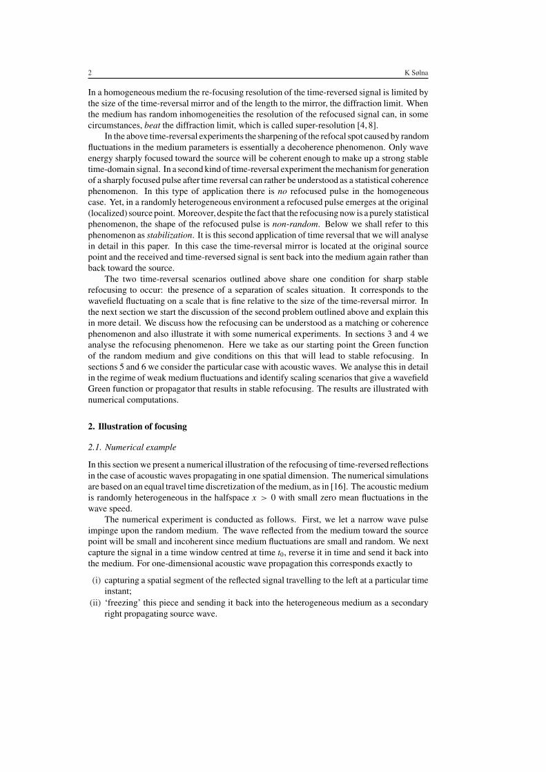
Figure 1. This figure shows the refocusing at the original source point for the second-orderreflections from the random medium.

The second-order reflection generated by this new source is shown in figure 1, a time t0 afterwe sent the signal into the heterogeneous medium. Note the focusing at the original sourcepoint for these second-order reflections. This is what we referred to as refocusing above. Therefocusing is no coincidence. If we repeat the experiment with a different realization of therandom medium we will see essentially the same refocused pulse. This is what we referred toas stable refocusing above. We next aim to describe qualitatively why this happens.

2.2. Response matching via time-reversal

To explain and quantify the focusing seen above we repeat the steps and illustrate it with someschematic cartoons.

The medium is heterogeneous in a halfspace, the halfspace x > 0, and homogeneous inthe other half, as before. We use first an impulsive source located at the origin at time zero andimpinging upon the random medium, see figure 2 top. The bottom plot shows the first-orderreflections from the random medium at time t0 (call them G(x)). Since we used an impulsivesource, the process G(x) can be interpreted as the impulse response function of the medium orits random Green function. We refer to the scale at which G fluctuates as l. Thus, we assumethat G(x) and G(x +�x) are approximately independent if l � |�x | and strongly correlatedif |�x | � l.

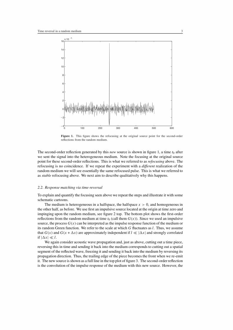
We again consider acoustic wave propagation and, just as above, cutting out a time piece,reversing this in time and sending it back into the medium corresponds to cutting out a spatialsegment of the reflected wave, freezing it and sending it back into the medium by reversing itspropagation direction. Thus, the trailing edge of the piece becomes the front when we re-emitit. The new source is shown as a full line in the top plot of figure 3. The second-order reflectionis the convolution of the impulse response of the medium with this new source. However, the

4 K Sølna

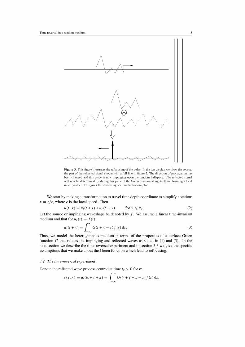
Figure 2. This figure illustrates the first-order reflections from an impulsive source. The top displayshows the impinging impulse travelling to the right in the homogeneous halfspace and impingingupon the random or heterogeneous right halfspace. The bottom display shows the reflections, therandom Green function or impulse response of the medium, evaluated a time t0 later. The part ofit that is shown with a full line is the part that corresponds to the window of width W , the segmentthat we capture, time-reverse and send back into the medium.

source was just a piece of the impulse response or Green function itself. Due to the fact thatwe time reversed before re-emitting the signal, the convolution corresponds to sliding a pieceof the Green function along itself and forming a local ‘inner product’, as illustrated in themiddle display of figure 3. Evaluating the second-order reflection at time t0 at the spatialorigin corresponds to the Green function and the piece being exactly coherent before we formthe inner product. Evaluating the reflection at time t0, but a distance more than l from theorigin corresponds to complete decoherence and a small inner product, thus giving re-focusingas in figure 3 (bottom plot) of a pulse that is moving to the left. The support of the refocusedpulse will be O(l). To quantify the relative magnitude of the refocused pulse, assume thatXn = G(ln) are zero mean, independently and identically distributed random variables. Letalso N = W/ l with W the width of the window. The magnitude of the fluctuations relative tothe refocused pulse is then of the order of√

Var[∑N

i=1 Xi Xi+�]

E[∑N

i=1 X2i ]

= O(N−1/2).

Thus, the focusing phenomenon in time reversal is due to the matching of two copies of theresponse function of the (time-invariant) medium. It will occur when we have a separation ofscales, in that the window width is large relative to the scale at which the response functiondecorrelates. The more detailed analysis carried out below confirms this picture.

3. Waves over a layered medium

3.1. The Green function

We analyse the focusing phenomenon in a one-dimensional medium. The randomheterogeneous medium is located in the halfspace z > z0. In the homogeneous halfspacewe assume that the wave, u, can be decomposed as

u(t, z) = ul(t + z/c0) + ur (t − z/c0) for z � z0, (1)

with c0 being the wave speed.

Time reversal in a random medium 5

Figure 3. This figure illustrates the refocusing of the pulse. In the top display we show the source,the part of the reflected signal shown with a full line in figure 2. The direction of propagation hasbeen changed and this piece is now impinging upon the random halfspace. The reflected signalwill now be determined by sliding this piece of the Green function along itself and forming a localinner product. This gives the refocusing seen in the bottom plot.

We start by making a transformation to travel time depth coordinate to simplify notation:x = z/c, where c is the local speed. Then

u(t, x) = ul(t + x) + ur (t − x) for x � x0. (2)

Let the source or impinging waveshape be denoted by f . We assume a linear time-invariantmedium and that for ur (t) = f (t):

ul(t + x) =∫ ∞−∞

G(t + x − s) f (s) ds. (3)

Thus, we model the heterogeneous medium in terms of the properties of a surface Greenfunction G that relates the impinging and reflected waves as stated in (1) and (3). In thenext section we describe the time-reversal experiment and in section 3.3 we give the specificassumptions that we make about the Green function which lead to refocusing.

3.2. The time-reversal experiment

Denote the reflected wave process centred at time t0 > 0 for r :

r(τ, x) ≡ ul(t0 + τ + x) =∫ ∞−∞

G(t0 + τ + x − s) f (s) ds.

6 K Sølna

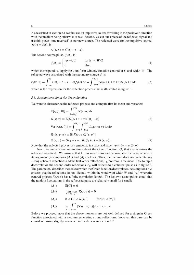
As described in section 2.1 we first use an impulsive source travelling in the positive x directionwith the medium being otherwise at rest. Second, we cut out a piece of the reflected signal anduse this piece ‘time reversed’ as our new source. The reflected wave for the impulsive source,f1(t) = δ(t), is

r1(τ, x) = G(t0 + τ + x).

The second source pulse, f2(t), is

f2(t) ={

r1(−t, 0) for |t| < W/2

0 else,(4)

which corresponds to applying a uniform window function centred at t0 and width W . Thereflected wave associated with the secondary source f2 is

r2(τ, x) =∫ ∞−∞

G(t0 + τ + x − s) f2(s) ds =∫ W/2

−W/2G(t0 + τ + x + s)G(t0 + s) ds, (5)

which is the expression for the reflection process that is illustrated in figure 3.

3.3. Assumptions about the Green function

We want to characterize the reflected process and compute first its mean and variance:

E[r2(σ, 0)] =∫ W/2

−W/2R(s; σ) ds

R(s; σ) ≡ E[G(t0 + s + σ)G(t0 + s)] (6)

Var[r2(σ, 0)] =∫ W/2

−W/2

∫ W/2

−W/2R2(s, v; σ) ds dv

R2(s, v; σ) ≡ E[X (s; σ)X (v; σ)]X (s; σ) ≡ G(t0 + s + σ)G(t0 + s)−R(s; σ). (7)

Note that the reflected process is symmetric in space and time: r2(σ, 0) = r2(0, σ ).Next, we make some assumptions about the Green function, G, that characterizes the

reflected wavefield. We assume that G has mean zero and decorrelates for large offsets inits argument (assumptions (A1) and (A2) below). Thus, the medium does not generate anystrong coherent reflections and the first-order reflections, r1, are zero in the mean. Due to rapiddecorrelation the second-order reflections, r2, will refocus to a coherent pulse as in figure 3.The parameter l describes the scale at which the Green function decorrelates. Assumption (A3)

ensures that the reflections do not ‘die out’ within the window of width W and (A4) wherethecentred process X (s; σ) has a finite correlation length. The last two assumptions entail thatthe random fluctuations in the refocused pulse are relatively small for l small:

(A1) E[G] = 0

(A2) limσ→∞ sup

s|R(s; σ)| = 0

(A3) 0 < C1 < R(s, 0) for |s| < W/2

(A4) sups,σ

∫ ∞−∞|R2(s, v; σ)| dv = l <∞.

Before we proceed, note that the above moments are not well defined for a singular Greenfunction associated with a medium generating strong reflections: however, this case can beconsidered using slightly smoothed initial data as in section 3.7.

Time reversal in a random medium 7

3.4. Focusing in the mean

The above modelling gives trivially that the second-order reflection, r2, focuses (in the mean):

Result 1. The assumptions (A1,...,3) imply that ∀δ > 0 ∃M > 0 such that

E[r2(σ, 0)]

E[r2(0, 0)]< δ for σ > M.

Note that the focusing is symmetric in the space and time dimensions.

3.5. Separation of scales and stabilization

The modelling moreover easily gives that the random fluctuations in the reflection process aresmall relative to the magnitude of the focused pulse for large relative window width. This iswhat we refer to as stabilization:

Result 2. The assumptions (A1,...,4) imply that√Var[r2(σ, 0)]

E[r2(0, 0)]� 1

C1√

Nwith N ≡ W/ l.

In the special case that G(t) and G(t + τ) are independent for |τ | > l, then (A2) and (A4) aresatisfied forR2 bounded. If, moreover, l � W the separation of timescales that we discussedin the introduction is present and we get stable refocusing.

3.6. Local stationarity

In this section we introduce some additional assumptions to get a more precise characterizationof the focused reflections. We consider the case when the random fluctuations in r2 are rapidrelative to the window width, but when the statistics of the reflection process vary slowly relativeto this scale. Thus, the window width separates the micro- and the macroscale in the reflectionprocess. We make here the idealized stationarity assumption: the process G(t0 +s +σ)G(t0 +s)is nearly stationary in s when observed for |s| < W . Then we find

E[r2(σ, 0)] =∫ W/2

−W/2R(s, σ ) ds ≈ WR(0, σ ) (8)

and approximately:√

Var[r2(σ, 0)]

E[r2(0, 0)]<

√∫∞−∞ |R2(0, v; σ)|/(R(0, 0))2 dv

W.

Thus, the shape of the refocused pulse isR(0, σ ), the covariance function of the Green functionevaluated relative to the centre of the time window. The relative magnitude of the fluctuationsin the refocused pulse is bounded in terms of the correlation length of the process X relativeto the window width.

3.7. General source and window functions

Consider now the more general case with a smooth source function, f1(t) = f (t), supportedon an intervalO(d)with d � W and normalized such that || f ||1 = 1. Moreover, we introducea window functionW(t), supported for |t| < W/2, so that the secondary source as in (4) is

f2(t) ={

r1(−t, 0)W(−t) for t < W/2

0 else.

8 K Sølna

In this case

r2(τ, x) =∫ ∞−∞

G(t0 + τ + x + s)W(s)∫ ∞−∞

G(t0 + s − v) f (v) dv ds

and

E[r2(σ, 0)] =∫ ∞−∞

∫ ∞−∞W(s + v)R(s, σ + v) f (v) dv ds. (9)

Under the stationarity assumptions of the previous section we find

E[r2(σ, 0)] ≈ [R(0, ·) f (−·)](σ )∫ ∞−∞W(s) ds (10)

with representing convolution. If we then assume that the Green function is mixing on thescale l we find √

Var[r2(σ, 0)]

E[r2(0, 0)]= O

(√max(l, d)

W

).

Thus, the reflections focus at the origin for time t0. If l � d, then the support of the focusedpulse is approximately that of the source pulse and the relative fluctuations of the order ofO(√

d/W ).

4. Three-dimensional effects

We summarize how the focusing generalizes to a two- or three-dimensional (time-invariant)medium. Analysis for a point source located over a layered medium is presented in [2]. Theheterogeneous random medium is located in the halfspace z > z0 > 0. We assume that thereis one lateral spatial dimension, denoted x ; the three-dimensional case is analogous. Thesource is located at (z, x) = (0, xs) and we record the reflected field at the point of observation(z, x) = (0, xo). We again state the assumptions regarding the medium and the propagationphenomenon in terms of the Green function G = G(t, xs, xo). As in the one-dimensional casewe express the reflections observed at the surface z = 0 in terms of a Green function:

u(t, xo, xs) =∫ ∞−∞

G(t − s, xo, xs) f (s) ds, (11)

with f being the source function.We next describe the time-reversal experiment which is analogous to the experiment in the

one-dimensional case. However, in this case we consider different source and receiver points.First, we use an impulsive source at the source point xs . Next, we observe the reflections at xo

in a time segment around t0 and use this segment, reversed in time, as a new source functionwith source location xo. As we will show, a focused pulse will then emerge at xs a time periodt0 after re-emission. Denote the reflections associated with the impulsive source r1 by

r1(τ ) = G(t0 + τ, xo, xs).

The secondary source located at xo is

f2(t) ={

r1(−t, 0) for t < W/2

0 else.

The reflections observed at a point in the vicinity of the original source point, (z, x, t) =(0, xs +�x, t0 + τ), are

r2(τ,�x) =∫ W/2

−W/2G(t0 + s + τ, xs +�x, xo)G(t0 + s, xo, xs) ds.

Time reversal in a random medium 9

Again we seek a characterization of the second-order reflections and compute the meanand variance for these:

E[r2(τ,�x)] =∫ W/2

−W/2R(s; τ,�x) ds

R(s; τ,�x) ≡ E[G(t0 + s + τ, xs +�x, xo)G(t0 + s, xo, xs)]

Var[r2(τ,�x)] =∫ W/2

−W/2

∫ W/2

−W/2R2(s, v; τ,�x) ds dv

R2(s, v; τ,�x) = E[X (s; τ,�x)X (v; τ,�x)]

X (s; τ,�x) = G(t0 + s + τ, xs +�x, xo)G(t0 + s, xo, xs)−R(s; τ,�x).

We now make a set of assumptions about the statistical moments of the Green function.Assumption (B1) below entails that the medium does not generate any strong coherentreflections. The essential aspect of the random field G that gives refocusing of the second-order reflections is that it decorrelates rapidly in space and time, assumption (B2) below. Asbefore, assumption (B3) entails that the reflections do not ‘die out’ within the time window.The condition (B4) ensures that the centred process X (s; τ,�x) has a finite correlation lengthand gives stabilization in the case that the window width is large relative to this length l:

(B1) E[G] = 0

(B2) limτ→∞ sup

s,�x|R(s; τ,�x)| = 0

lim�x→∞ sup

s,τ|R(s; τ,�x)| = 0

(B3) 0 < C2 < R(s; 0, 0) for |s| < W

(B4) sups,τ,�x

∫ ∞−∞|R2(s, v; τ,�x)| dv = l <∞.

These assumptions give refocusing:

Result 3. The assumptions (B1,...,3) imply that ∀δ > 0 ∃M > 0 such that

E[r2(τ,�x)]

E[r2(0, 0)]< δ for min(|τ |, |�x |) > M.

Therefore, at the surface z = 0 the mean reflection focuses at the original source point fortime t = t0. The support in time, (τ ), and space, (�x), of the refocused pulse will be onthe scale at which R decorrelates in these variables. The stabilization property seen in theone-dimensional case prevails:

Result 4. The assumptions (B1,...,4) imply that√Var[r2(τ,�x)]

E[r2(0, 0)]� 1

C2√

Nwith N ≡ W/ l.

Note that if the Green function satisfies the reciprocity property:

G(t, xs, xo) = G(t, xo, xs),

then

R(s; τ,�x) = E[G(t0 + s + τ, xs +�x, xo)G(t0 + s, xs , xo)]

and the above assumptions correspond to the Green function decorrelating rapidly in the sourcecoordinates.

10 K Sølna

5. Acoustic waves

5.1. Refocusing in the acoustic case

In this section we consider the acoustic case with the random medium fluctuations modelledby stochastic processes. The governing equations are the conservation laws for momentumand mass:

ρ(x)∂

∂tu(t, x) +

∂

∂xp(t, x) = 0,

1

K (x)

∂

∂tp(t, x) +

∂

∂xu(t, x) = 0 (12)

with p(t, x) being pressure and u(t, x) velocity. The material parameters ρ and K are,respectively, the density and bulk modulus. We let L denote the macroscale in our problem.This length scale corresponds to the propagation distance for the signal in between emissionand recording times. The ‘microscale’ corresponds the characteristic spatial scale at which themedium fluctuates. We take this scale to be εL with ε a dimensionless small parameter. Themedium model is

ρ(x) ={ρ0

[1 +√εη( x

εL

)]for x > 0

ρ0 else,

1

K (x)=

1

K0

[1 +√εν( x

εL

)]for x > 0

1

K0else

(13)

where the random fluctuations c1 < ν < c2 and c3 < η < c4 are mean zero stationarystochastic processes and the halfspace x � 0 is homogeneous. In section 6 we consider themore general case when the mean density ρ0 = ρ0(x) and the mean bulk modulus K0 = K0(x)are assumed to be differentiable functions of x . The above model is the one introduced andanalysed in [5], the difference being the factor

√ε multiplying the random fluctuations. Thus,

we consider here a weakly fluctuating medium whereas the analysis presented in [5] concernsa strongly fluctuating medium. The smooth, compactly supported in [0,∞) source wavelet is

f1(t) = f

(t

ε

).

Observe that we let the source pulse be supported on the microscale. Hence there will be astrong interaction between the pulse and the microscale medium variations. The small-scalenoise in the medium model gives a non-coherent backscattering. As discussed above, thesewe capture in a time window and use as a secondary source wavelet, after time reversal. In thehomogeneous halfspace we can decompose the wavefield as

u = [ f1(t − x/c0) + g(t + x/c0)]/ζ0

p = f1(t − x/c0) + g(t + x/c0),

with ζ0 = √K0ρ0 being the acoustic impedance and c0 = ζ0/ρ0 the acoustic sound velocityin this halfspace. Thus, the initial boundary condition that gives the primary source, a left-travelling wave pulse that strikes x = 0 at time t = 0, is

u = f1(t − x/c0)

ζ0

p = f1(t − x/c0)

Time reversal in a random medium 11

for t � tm . We write the first-order reflections generated by this source as

r1(τ ) = p(t0 + τ, 0) = [G f1](t0 + τ),

with G being the surface Green function. We capture these reflections in a window and thenreverse time to get the secondary source:

f2(−t) ≡ r1(t)W(t)

withW being a window function and defined as before. The initial boundary condition withthe secondary source is

u2 = f2(t − x/c0)

ζ0

p2 = f2(t − x/c0),

for t � tm . The corresponding secondary reflections become

r2(τ ) = p2(t0 + τ, 0) = [G f2](t0 + τ) = [G(·) [G f1](t0 − ·)W(−·)](t0 + τ).

This wavefield refocuses stably for small τ . We show in section 6:

Result 5. Assume that η(s) and ν(s) are bounded, stationary ergodic Markov processes, thenin probability

limε→0

r2(εσ ) =∫ ∞−∞

∫ ∞−∞R(s, σ + v)W(s) f (v) dv ds

as in (9) and (22). The function R can formally be interpreted as the covariance of the Greenfunction:

R(s, σ ) = limε→0

E[G(t0 + s + εσ )G(t0 + s)],

and is given by

R(s, σ ) = 1

2π

∫ω2α(2ω)

(1 + ω2α(2ω)2(t0 + s)/tL )e−iωσ/tL dω (14)

with tL = L/c0 and α being the power spectral density of the medium fluctuations:

α(ω) =∫ ∞

0α(s) cos(ωs) ds ≡

∫ ∞0E

[η(s) + ν(s)

2

]cos(ωs) ds.

Note that the surface Green function therefore decorrelates on the scale ε.Consider now the case with the medium model:

ρ(x) ={ρ0l[1 +√εδη

( x

εL

)]for x > 0

ρ0 else

1

K (x)=

1

K0

[1 +√εδν

( x

εL

)]for x > 0

1

K0else,

with ε � δ � O(1). Thus, the medium fluctuations are weaker than in the case we consideredabove. The above result prevails in this case when t0 �→ t0/δ andW(·) �→W(δ·). Thus, for ahomogeneous medium the shape of the refocused pulse is essentially not affected by δ if t0 isreplaced by t0/δ such that the wave penetrates deeper into the medium to compensate for theweaker fluctuations.

12 K Sølna

Consider finally the case with δ small and t0 fixed. Then

limε→0

r2(εσ ) ∝ [α(·/2) f ′′(·)](−σ) (15)

and in the low frequency case with f being smooth relative to the support of α:

limε→0

r2(εσ ) ∝ f ′′(−σ).

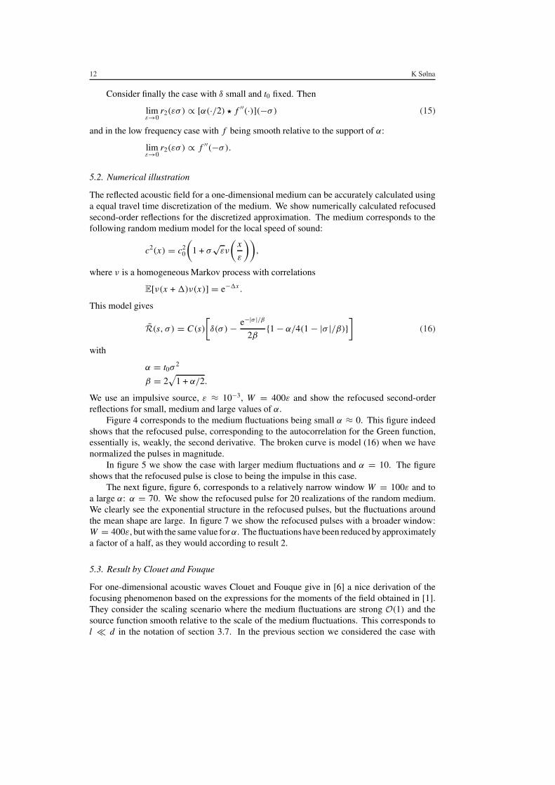
5.2. Numerical illustration

The reflected acoustic field for a one-dimensional medium can be accurately calculated usinga equal travel time discretization of the medium. We show numerically calculated refocusedsecond-order reflections for the discretized approximation. The medium corresponds to thefollowing random medium model for the local speed of sound:

c2(x) = c20

(1 + σ√εν

(x

ε

)),

where ν is a homogeneous Markov process with correlations

E[ν(x +�)ν(x)] = e−�x .

This model gives

R(s, σ ) = C(s)

[δ(σ )− e−|σ |/β

2β{1− α/4(1− |σ |/β)}

](16)

with

α = t0σ2

β = 2√

1 + α/2.

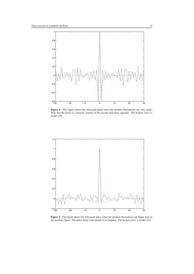
We use an impulsive source, ε ≈ 10−3, W = 400ε and show the refocused second-orderreflections for small, medium and large values of α.

Figure 4 corresponds to the medium fluctuations being small α ≈ 0. This figure indeedshows that the refocused pulse, corresponding to the autocorrelation for the Green function,essentially is, weakly, the second derivative. The broken curve is model (16) when we havenormalized the pulses in magnitude.

In figure 5 we show the case with larger medium fluctuations and α = 10. The figureshows that the refocused pulse is close to being the impulse in this case.

The next figure, figure 6, corresponds to a relatively narrow window W = 100ε and toa large α: α = 70. We show the refocused pulse for 20 realizations of the random medium.We clearly see the exponential structure in the refocused pulses, but the fluctuations aroundthe mean shape are large. In figure 7 we show the refocused pulses with a broader window:W = 400ε, but with the same value forα. The fluctuations have been reduced by approximatelya factor of a half, as they would according to result 2.

5.3. Result by Clouet and Fouque

For one-dimensional acoustic waves Clouet and Fouque give in [6] a nice derivation of thefocusing phenomenon based on the expressions for the moments of the field obtained in [1].They consider the scaling scenario where the medium fluctuations are strong O(1) and thesource function smooth relative to the scale of the medium fluctuations. This corresponds tol � d in the notation of section 3.7. In the previous section we considered the case with

Time reversal in a random medium 13

– 30 – 20 – 10 0 10 20 30– 0.6

– 0.4

– 0.2

0

0.2

0.4

0.6

0.8

1

Figure 4. This figure shows the refocused pulse when the medium fluctuations are very small.Note that the pulse is a discrete version of the second derivative operator. The broken curve ismodel (16).

– 30 – 20 – 10 0 10 20 30– 0.2

0

0.2

0.4

0.6

0.8

1

1.2

Figure 5. This figure shows the refocused pulse when the medium fluctuations are larger than inthe previous figure. The pulse shape corresponds to an impulse. The broken curve is model (16).

14 K Sølna

– 30 – 20 – 10 0 10 20 300. 4

0.2

0

0.2

0.4

0.6

0.8

1

–

–

Figure 6. This figure displays refocused pulses for several independent realizations of the randommedium. The window width, W , is small and the fluctuations in the pulse shapes large. The fullcurve is the average pulse shape.

– 30 – 20 – 10 0 10 20 30– 0.4

– 0.2

0

0.2

0.4

0.6

0.8

1

Figure 7. This figure displays refocused pulses for several independent realizations of the randommedium. The window width, W , is larger than in the previous figure and the fluctuations in thepulse shapes smaller. Thus, the figure illustrates the stability in the pulse shape with respect to theparticular medium realization for large window widths. The broken curve is model (16) and thefull curve the average pulse shape.

Time reversal in a random medium 15

l ≈ d and hence a stronger interaction of the pulse with the statistics of the medium. We hereconnect their result to the above. Let the governing equations be (12) with model parameters

ρ(x) ={(K /c2

0)[1 + η

( x

ε

)]for x > 0

(K /c20) else,

K (x) ≡ K

and initial source function

f1(t) = f

(t√ε

).

It is shown in [6] that the second-order reflections can then be expressed as

limε→0

E[r2(t0 +√εσ )] =

∫ ∞−∞

e−iωσ f (ω)[�(ω, t) G(t)](t0) dω (17)

with

�(ω, t) = ω2α(0)

(1 + ω2α(0)t0)2. (18)

This expression can be rewritten in the form (9) with R the transform of � and with the longwavelength limit of (14) matching the weak noise limit of (17).

5.4. Connection to localization

The form

ω2σ 2

(1 + ω2σ 2t0)2(19)

for the local power spectrum of the Green function corresponds to the above and entails thatthe refocused pulse is approximately

σ 2 f ′′

for t0 small. We give next a heuristic motivation. With t0 small mostly first-order scatteringevents close to the surface contribute to the reflected signal. Consider a discrete approximationof the medium. Then a large interface reflection coefficient of magnitude, say σ , is followedby a second of approximately opposite magnitude,−σ . With the probing pulse being smoothrelative to the fluctuations this means that the backscattered signal scales like σ f ′. The second-order time-reversed signal thus scales like σ 2 f ′′. A correction to this picture can be obtainedby recalling that the frequency-dependent localization length in the above acoustic case isapproximately

lloc = c0

2ω2σ 2.

This suggest the following approximation for the ‘transmission loss’ for the first-orderreflections from a shallow depth L = c0t0/2:

e−L/lloc ≈ 1

1 + ω2σ 2t0.

A local ‘reflexivity’ σω, together with this transmission loss, suggest the form (19) for thepower spectrum.

16 K Sølna

6. Derivation for acoustic waves

6.1. Problem formulation

We summarize here the derivation of result 5 for the refocused pulse in the acoustic case withweak medium fluctuations. The method used is the one set forth in [5] adapted to the casewith weak medium fluctuations and a probing pulse that is supported on the microscale ratherthan being smooth relative to this scale. We consider the model defined by (12) and let theparameters be defined by

ρ(x) =ρ0

( x

L

)[1 +√εη( x

εL

)]for x > 0

ρ0(0) else

1

K (x)=

1

K0(x/L)

[1 +√εν( x

εL

)]for x > 0

1

K0(0)else.

(20)

The mean density ρ0 and the mean bulk modulus K0 are assumed to be differentiable functionsof x . Following [5] we non-dimensionalize by setting

x ′ = x

Lp′ = p

ρ0(0)c0(0)2

t ′ = c0(0)t

Lu′ = u

c0(0)

ρ ′0(x′) = ρ0(x ′)

ρ0(0)K ′0(x

′) = K0(x ′)K0(0)

.

After dropping primes we find in non-dimensionalized units

ρ(x)∂

∂tu(t, x) +

∂

∂xp(t, x) = 0,

1

K (x)

∂

∂tp(t, x) +

∂

∂xu(t, x) = 0

with ρ0(x) ≡ 1, K0(x) ≡ 1 and c0(x) ≡ 1 for x � 0. Next, we Fourier transform in time as

u(ω, x) =∫

eiωt/εu(t, x) dt

p(ω, x) =∫

eiωt/ε p(t, x) dt

and introduce the ‘travel time’ from the origin according to the smooth background mediumby

τ(x) =∫ x

0

ds

c0(s).

We also decompose in left-going, A, and right-going, B, waves:

u = 1

(K0ρ0)1/4[Ae−iωτ/ε + Beiωτ/ε]

p = (K0ρ0)1/4[−Ae−iωτ/ε + Beiωτ/ε]

with the decomposition being defined according to the smooth background medium. Anincoming impulse at x = 0 corresponds to B1(ω) = B(0;ω) ≡ 1 and then the transformedGreen function is G(ω) = R(0;ω) = A(0;ω), where we introduced the reflection coefficientR = A/B. In section 6.3 we discuss further the equation and boundary conditions for R andobtain a characterization of the Green function G.

Time reversal in a random medium 17

6.2. First- and second-order reflections

First, let the source wavelet be

f1(t) = f (t/ε)

with Fourier transform

f (ω) =∫

eiωt f (t) dt .

This is the probing right-going source when evaluated at the origin x = 0 and corresponds toB1(ω) = ε f (ω). We choose a scaling such that the source wavelet is O(1) in magnitude, butthis choice is not important as the problem is linear. The first-order reflection, the left-goingwavelet, generated by the source and evaluated at x = 0 is

r1(t) = 1

2πε

∫G(ω)B1(ω)e

−iωt/ε dω = 1

2π

∫G(ω) f (ω)e−iωt/ε dω.

We capture the reflections at time t0 and apply the window functionW before we time reverseto get the secondary source wavelet:

f2(t) = r1(t0 − t)W(−t),

which corresponds to

B2(ω) = 1

2π

∫G(−(ω + εh)) f (−(ω + εh))W(h)eit0(h+ω/ε) dh.

The reflections associated with this second right-going source wavelet is, when evaluated atx = 0,

r2(t) = 1

2π

∫G(ω)A2(ω)e−iωt/ε dω

= 1

(2π)2

∫G(ω − εh)G(−ω) f (−ω)W(h)eiω(t0−t)/εeiht dω dh,

with W being the unscaled Fourier transform ofW . We introduce next the spectrum

�(t, ω) = 1

2π

∫E[G(ω − εh)G(−ω)]eiht dh. (21)

The mean reflected process can then be written as

E[r2(t)] = 1

2π

∫�(t − s, ω)W(−s) ds eiω((t0−t)/ε−τ) dω f (τ ) dτ.

In the next section we shall obtain an explicit expression for the power spectrum �. Weintroduce also

R1(t, s) = 1

2πε

∫�(t, ω)e−iωs/ε dω.

The expression for the mean reflected pressure is then

E[r2(t)] = ε∫R1(t − s, t − t0 + ετ)W(−s) ds f (τ ) dτ

=∫R1(t − s, t − t0 + τ)W(−s) ds f1(τ ) dτ.

It follows from the result of the next section that R1 has supportO(ε) in its second argumentwhich is the scale of the correlation length of the medium. Thus, only if t − t0 = O(ε) willwe see a refocused pulse. For t = t0 + εσ we find

E[r2(t0 + εσ )] =∫R1(t0 + εσ − s, εσ + τ)W(−s) ds f

(τ

ε

)dτ. (22)

18 K Sølna

Thus, first the statistics of the ‘locally stationary’ covariance of the Green function is averagedwith respect to the window function, then this mean covariance is averaged with respect to thesource wavelet. The source wavelet is chosen to be supported on the scale at which the Greenfunction decorrelates. Formally we have

R1(t0 + t, s) = E[G(t0 + t)G(t0 + t − s)] = R(t,−s)

with R defined as in (6). Hence

E[r2(t0 + σ)] =∫ ∞−∞

∫ ∞−∞W(s + v)R(s, σ + v) f1(v) dv ds,

which is (9).

6.3. The power spectrum

We summarize here how the expression for �(t, ω) introduced in (21) can be derived. Thisexpression, corresponding to the autocorrelation of the surface Green function, defines the(mean) shape of the refocused pulse. In the next subsection we discuss stabilization (i.e. therandom fluctuations in the refocused pulse are small). The argument as presented here isformal. However, steps involving interchange of limits and choice of boundary conditions canbe made rigorous using the method of functionals introduced in [5, 13].

We seek an expression for

R(ω, h) ≡ E[G(ω − εh/2)G(ω + εh/2)].

Then

�(t, ω) = 1

2π

∫R(ω − εh/2, h)eiht dh ∼ 1

2π

∫R(ω, h)eith dh as ε ↓ 0. (23)

Recall that G(ω) = R(0;ω), with R = A/B being the reflection coefficient introduced above.From (12) and (20) it follows that the equations for the ‘right/left-going’ amplitudes are

d

dx

[AB

]= iω√

ε

(ρ0

K0

)1/2 [ −m −ne2iωτ/ε

ne−2iωτ/ε m

] [AB

]

+1

4

(K0ρ0)′

(K0ρ0)

[0 e2iωτ/ε

e−2iωτ/ε 0

] [AB

]with

m = (η + ν)/2

n = (η − ν)/2.This gives a Ricatti equation for the reflection coefficient:

dR

dx= −iω√

ε

(ρ0

K0

)1/2

[ne2iωτ/ε + 2m R + n R2e−2iωτ/ε] +1

4

(ρ0 K0)′

(ρ0 K0)[e2iωτ/ε − R2e−2iωτ/ε].

(24)

It remains to choose boundary conditions for R. For a statistically homogeneous medium thewave cannot penetrate to infinite depth and as in [5] we choose a ‘totally reflecting termination’when analysing (24). That is, we write

R(x, ω) = e−iψ(x,ω)

with ψ real. This can be justified by embedding a finite section of the medium in a largestatistically homogeneous section where the wave localizes, so that asymptotically R has unit

Time reversal in a random medium 19

modulus, and finally truncate by a homogeneous section where a physical boundary conditionfor R can be imposed. This we can do without changing the solution due to hyperbolicityof the original problem. The method of functionals referred to above does not require suchassumptions about the whole medium as it works in the time domain.

Let ψ1,2(x, ω) = ψ(x, ω ∓ εh/2), then

R = E[ei(ψ2(0,ω)−ψ1(0,ω))]. (25)

We shall approximate this expectation by integrating with respect to the distribution ofψ2−ψ1

in the small ε limit corresponding to scattering associated with the random medium taking placeon a very fine scale.

For � = [ψ1, ψ2] we can write

d�

dx= ε−1 F(�) + G(�), (26)

with F = [F1, F2], G = [G1,G2] and

F1 = 2ω√ε

√ρ0

K0[m + n cos(ψ1 + 2ωτ/ε − hτ)]

G1 = −1

2

(ρ0 K0)′

ρ0 K0sin(ψ1 + 2ωτ/ε − hτ)−√εh

√ρ0

K0[m + n cos(ψ1 + 2ωτ/ε − hτ)]

and F2, G2 defined similarly. Note that m, n have zero mean and thus F is centred with respectto their distribution. The asymptotic theory for systems of the form (26) is well known, seefor instance [1,5,12]. In [1,12] the case with a constant background medium was considered.Using the perturbation of generator approach as in [5] we can generalize this to the above case.The result is that if we make the change of variables

ψ = ψ2 − ψ1

ψ = 1/2(ψ2 + ψ1),

then we find that the associated infinitesimal generator in the small ε limit is

Lx (ω) = 4ω2

c20(x)

{αs,n(2c0(x)ω)/2

∂

∂ψ+ αc,n(2c0(x)ω)

[1

4

∂2

∂ψ2

+∂2

∂ψ2+ cos(ψ + 2hx)

(1

4

∂2

∂ψ2− ∂2

∂ψ2

)]+ α

∂2

∂ψ2

}(27)

with

α =∫ ∞

0E[m(0)m(s)] ds

αc,n(ω) =∫ ∞

0E[n(0)n(s)] cos(ω) ds

αs,n(ω) =∫ ∞

0E[n(0)n(s)] sin(ω) ds.

The coefficients in (27) do not depend on ψ and hence ψ is Markovian by itself. We nowspecialize to the case with uniform background and c(x) ≡ 1. Then we can solve the backwardKolmogorov equation associated with (27) explicitly:

∂V

∂x− 4ω2αc,n(2ω)(1− cos(ψ + 2hx))

∂2

∂ψ2V = 0.

20 K Sølna

In view of 25 we find that

R = limx→∞ V (x, ψ),

when

V |x=0 = eiψ .

The limit does not depend on ψ and using (23) we get the desired result (14). The generalcase with c0 = c0(x) leads to an infinite-dimensional system of equations similar to the systemderived in [5].

6.4. Stabilization

The stabilization of the refocused pulse follows as in [4,15] if we can show that the quadraticGreen operator R decorrelates for different frequencies:

R(ωa, ωb) = E[ei(ψ2(0,ωa)−ψ1(0,ωa))ei(ψ2(0,ωb)−ψ1(0,ωb))]

∼ E[ei(ψ2(0,ωa)−ψ1(0,ωa))]E[ei(ψ2(0,ωb)−ψ1(0,ωb))] as ε ↓ 0. (28)

Then the second centred moment of the refocused pulse is small in the small ε limit. Ifwe define �2(ωa, ωb) = [ψ(ωa), ψ(ωa)ψ(ωb), ψ(ωb)], then the associated infinitesimalgenerator becomes

Lx (ωa, ωb) = Lx (ωa) + Lx(ωb)− ωaωbα∂

∂ψa

∂

∂ψb

.

Since the infinitesimal generator associated with�2 is the sum of the ones associated with thesingle-frequency cases up to a differential term in ψa and ψb we find that (28) is satisfied andthat the fluctuations in the refocused pulse are relatively small.

7. Conclusions

We have analysed refocusing of time-reversed wave reflections. In this problem the presenceof several scales is important, as well as how these separate. We gave a simple interpretation ofhow stable refocusing can be interpreted in terms of averaging and illustrated it with numericalsimulations. We analysed in detail acoustic waves and characterized precisely the refocusingin this case using limit theorems for stochastic ordinary differential equations.

Acknowledgments

This work was supported by NSF grant DMS-0093992 and ONR grant N00014-02-1-0090.

References

[1] Ash M, Kohler W, Papanicolaou G C, Postel M and White B 1991 Frequency content of randomly scatteredsignals SIAM Rev. 33 519–625

[2] Bailly F and Fouque J P Preprint See endnote 2[3] Berryman J, Borcea L, Papanicolaou G and Tsogka C Imaging in noisy environments Preprint See endnote 3

See endnote 4[4] Blomgren P, Papanicolaou G and Zhao H Super-resolution in time-reversal acoustics J. Acoust. Soc. Am. at press

See endnote 5[5] Burridge R, Papanicolaou G, Sheng P and White B 1989 Probing a random medium with a pulse SIAM J. Appl.

Math. 49 582–607

Time reversal in a random medium 21

[6] Clouet J F and Fouque J P 1997 A time-reversal method for an acoustical pulse propagating in randomly layeredmedia Wave Motion 25 361–8

[7] Ing R K and Fink M 1995 Surface and sub-surface flaw detection using rayleigh wave time reversal mirrorsProc. IEEE Ultrason. 1 733–6

[8] Dowling D R and Jackson D R 1992 Narrow-band performance of phase-conjugate arrays in dynamic randommedia J. Acoust. Soc. Am. 91 3257–77

[9] Fink M 1999 Time-reversed acoustics Sci. Am. November 91–7[10] Fink M 1993 Time reversal mirrors J. Phys. D: Appl. Phys. 26 1333–50[11] Kuperman W A, Hodgkiss W S, Song H C, Akal T, Ferla C and Jackson D R 1997 Phase conjugation in the

ocean: experimental demonstration of an acoustic time-reversal mirror J. Acoust. Soc. Am. 103 25–40[12] Lewicki P and Papanicolaou G 1994 Reflection of wavefronts by randomly layered media Wave Motion 20

245–60[13] Papanicolaou G and Weinryb S 1994 A functional limit theorem for waves reflected by a random medium Appl.

Math. Opt. 30 307–34[14] Thomas J L and Fink M 1996 Ultrasonic beam focusing through tissue inhomogeneities with a time reversal

mirror: Application to transskull therapy IEEE Trans. Ultrason. Ferroelectr. Freq. Control 43 1122–9[15] Ryzhik L, Papanicolaou G C and Sølna K The parabolic approximation and time reversal in a random medium

Preprint See endnote 6[16] Sølna K 2001 Estimation of pulse shaping for well logs Geophysics 66 1605–11[17] Sølna K and Papanicolaou G 2000 Ray theory for a locally layered medium Waves Random Media 1 See endnote 7

Queries for IOP paper 133163

Journal: WRMAuthor: Knut SølnaShort title: Time reversal in a random medium

Page 1

Query 1:Author: Please be aware that the colour figures in this article will only appear in colour in

the Web version. If you require colour in the printed journal and have not previously arrangedit, please contact the Production Editor now.

Page 20

Query 2:Author: Preprint details for [2]?

Query 3:Author: Preprint details for [3]?

Query 4:Author: [3], [7] and [17] are not cited in text.

Query 5:Author: Publication details for [4]?

Page 21

Query 6:Author: Preprint details for [15]?

Query 7:Author: Page numbers for [17]?